GS434 Spring 98Lab Exercise I:Introduction to Matlab & Fourier AnalysisDue 1/27

Solutions

1. Compute and plot a simple sinusoid of amplitude 1 and frequency f=1 for0<t<1,

i.e. y= sin(2πft)

I wrote an m- file called sinusoid.m to compute and plot a simple sinusoid:

%An M file to compute and plot a simple sinusoidfreq =1;T= 1/f;npts=10;n = npts-1;dt = T/nt=0:dt:T;y=sin(2*pi*f*t);plot(t,y, '*')

What time step did you use to digitize the function? Why?

I originally selected dt to give me 10 pts between 0 and T. The resulting plotlooked like:

0 0.1 0.2 0.3 0.4 0.5 0.6 0.7 0.8 0.9 1-1

-0.8

-0.6

-0.4

-0.2

0

0.2

0.4

0.6

0.8

1

10 pts

10 pts.

Which wasn’t so bad.

What is the minimum time step you would use to represent this function?Plot the function with this time step.

I tried several values for npts from 8 to 3, for example

0 0.1

0.2

0.3 0.4 0.5

0.6

0.7

0.8

0.9

1-1

-0.8

-0.6

-0.4

-0.2

0

0.2

0.4

0.6

0.8

1

0 0.1 0.2 0.3

0.4

0.5 0.6

0.7

0.8 0.9 1-1

-0.8

-0.6

-0.4

-0.2

0

0.2

0.4

0.6

0.8

1

0 0.1

0.2

0.3

0.4 0.5 0.6 0.7

0.8

0.9

1-1

-0.8

-0.6

-0.4

-0.2

0

0.2

0.4

0.6

0.8

1

0 0.1 0.2 0.3

0.4

0.5

0.6

0.7

0.8

0.9

1-1

-0.8

-0.6

-0.4

-0.2

0

0.2

0.4

0.6

0.8

1

n=10 n=6

n=4 n=3

At least visually the plot loses all real definition below npts = 6. Notehowever, that according to the sampling theorem that we should be able toget by with only 3 pts.

2. Compute and plot a complex sinusoidal function consisting of the sum of 5sine waves with equal amplitudes but whose frequencies are 1,3,5,10, and20, again for t varying from 0 to 2π.

What time step did you use this time? Why?

Based on the experience above, I decided to use at 10 pts per shortest periodinvolved., i.e. Tshort = 1/20 = 0.05 or dt = 0.005.

I made an m file called fseries.m to plot the individual and compositesinusoids:

%sinsum% compute, combine and plot a set of simple sinusoids% first I load the desired frequencies and associated weightsf1=1;f2=3;

f3=5;f4=10;f5=20;% now I choose my sampling frequency to be equal to 10 times the highest

frequencyfsamp = 10*f5dt = 1/fsampnsamp=2*pi/dt% now I subsample (if required) by a factor of subsub=1dtsub=sub*dt%set max t to computetmax = 2*pi%now compute my time variablest=0:dtsub:tmax;%compute sinusoids and offset each oney1=sin(2*pi*f1*t);y2=sin(2*pi*f2*t)+2;y3=sin(2*pi*f3*t)+4;y4=sin(2*pi*f4*t)+6;y5=sin(2*pi*f5*t)+8;yall=(y1+y2+y3+y4+y5-20)/5+10;%plot sinusoidsplot(t,y1,t,y2,t,y3,t,y4,t,y5,t,yall)title(['dt=',num2str(dtsub)])

The resulting plot looked like:

0 1 2 3 4 5 6 7-2

0

2

4

6

8

10

12dt=0.005

Repeat the plot with a time step twice as large.

0 1 2 3 4 5 6 7-2

0

2

4

6

8

10

12dt=0.01

Since I oversampled greatly in the first place, my resampling by a factor of twodidn’t do much damage.

Repeat with a time step 10 times as large.

0 1 2 3 4 5 6 7-2

0

2

4

6

8

10

12dt=0.05

Now I have really aliased the two higher frequencies (to 0 as a matter of fact).

To look at this from another perspective, I also resampled by a factor of 8 toget:

0 1 2 3 4 5 6 7-2

0

2

4

6

8

10

12dt=0.04

This shows more clearly how the higher frequencies look like lowerfrequencies.

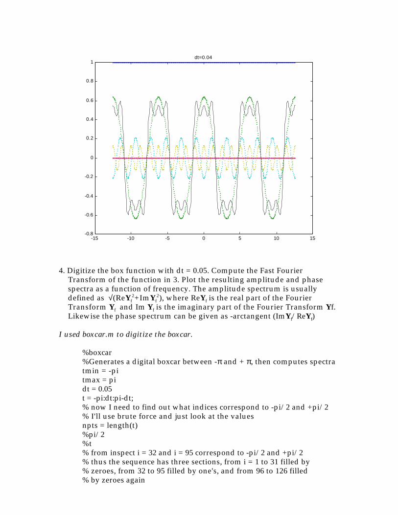
3. Compute and plot the first 5 terms of the Fourier series representation(page 277 in text), both individually and as a cumulative sum, for a simplebox function on the interval -π to +π:

y(t) = 0 for -π<t<-π/2 = 1 for -π/2<t<π/2

= 0 for π/2<t<π

We want to approximate this function by a series of sines and cosines, e.g. ∞

y(t) ~ a0/2 + ∑ (ancos(2πnft) + bnsin(2πnft)) (p. 277 of Sheriff and Geldart)

n = 1

For T = 2π the coefficients of the various sines and cosines are given by π π/2

an = (1/π) ∫-π

y(t) cos(nt)dt = (1/π) ∫

-π/2 1 . cos(nt)dt

and π π/2

bn = (1/π) ∫-π

y(t) sin(nt)dt = (1/π) ∫

-π/2 1 . sin(nt)dt

evaluating the integrals yields π/2

an = (1/π) [sin nt/n] -π/2

= (1/nπ)[sin(nπ/2)- sin(-nπ/2)]

or

an = (2/nπ) sin(nπ/2)= 2sin(nπ/2)/nπ

and π/2bn = (1/nπ) [-cos(nπ/2)]

-π/2 = -(1/nπ)[cos(nπ/2)-cos(-nπ/2)]

or

bn = 1(1//nπ) [cos(nπ/2)-cos(nπ/2)] = 0 for all n

That is there are now sinusoidal contributions, only co-sinusoidal.This is not surprising since the function we are trying to fit is symmetric (or

even).

By explicit evaluation, the first five coefficients are:

a0 = 2 sin(0)/0 = oops, this one gets a little tricky. If we refer to p. 531 we see

that we can back up a step and reduce the integral for n =0 to π/2 π/2

a0 = (1/π) ∫-π/2

1 . cos(0)dt = (1/π) ∫-π/2

1 . 1.dt = (1/π) (π/2-(-π/2))= 1

a1 = 2 sin(π/2)/π = 2/π

a2 = 2 sin(π)/2π = 0

a3 = 2 sin(3π/2)/3π = -2/3π

a4 = 2 sin(2π)/4π = 0

a5 = 2 sin(5π/2)/5π = 2/5π

so the first five terms of the Fourier Series are

y(t) ~ 1/2 + (2/π) cost - (3/2π) cos3t + (2/5π) cos5t

I can now use coseries.m to compute and plot the sum of these, i.e.

%coseries% compute, combine and plot a set of weighted cosines% first I load the desired frequencies and associated weightsf0=0; w0=1f1=1; w1=2/pif2=2; w2=0f3=3; w3=-2/(3*pi)f4=4; w4=0f5=5; w5=2/(5*pi)% now I choose my sampling frequency to be equal to 5 times thehighest frequencyfsamp = 5*f5dt = 1/fsampnsamp=2*pi/dt% now I subsample (if required) by a factor of subsub=1dtsub=sub*dt%set max and min t to computetmin = -4*pitmax = 4*pi%now compute my time variablest=tmin:dtsub:tmax;%compute sinusoids and offset each oney0=w0*cos(f0*t);y1=w1*cos(f1*t);y2=w2*cos(f2*t);y3=w3*cos(f3*t);y4=w4*cos(f4*t);y5=w5*cos(f5*t);yall=(y1+y2+y3+y4+y5);%plot sinusoidsplot(t, y0, '.',t,y1,'.',t,y2,'.',t,y3,'.',t,y4,'.',t, y5, '.', t,yall,'-')title(['dt=',num2str(dtsub)])

-4 -3 -2 -1 0 1 2 3 4-0.8

-0.6

-0.4

-0.2

0

0.2

0.4

0.6

0.8

1dt=0.04

What assumptions have you made about the behavior of y(t) outside theselimits?

I have assumed that it is periodic with period = 2π., i.e.

-15 -10 -5 0 5 10 15-0.8

-0.6

-0.4

-0.2

0

0.2

0.4

0.6

0.8

1dt=0.04

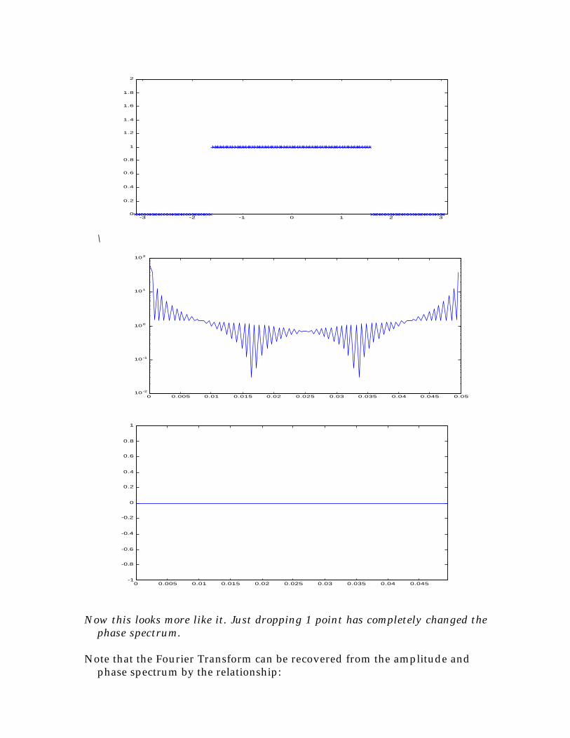
4. Digitize the box function with dt = 0.05. Compute the Fast FourierTransform of the function in 3. Plot the resulting amplitude and phasespectra as a function of frequency. The amplitude spectrum is usuallydefined as √(ReYf

2+ImYf2), where ReYf is the real part of the Fourier

Transform Yf and Im Yf is the imaginary part of the Fourier Transform Yf.Likewise the phase spectrum can be given as -arctangent (ImYf/ReYf)

I used boxcar.m to digitize the boxcar.

%boxcar%Generates a digital boxcar between -π and + π, then computes spectratmin = -pitmax = pidt = 0.05t = -pi:dt:pi-dt;% now I need to find out what indices correspond to -pi/2 and +pi/2% I'll use brute force and just look at the valuesnpts = length(t)%pi/2%t% from inspect i = 32 and i = 95 correspond to -pi/2 and +pi/2% thus the sequence has three sections, from i = 1 to 31 filled by% zeroes, from 32 to 95 filled by one's, and from 96 to 126 filled% by zeroes again

y1 = zeros(1,31);y2 = ones (1,64);y3 = zeros (1,31);%combine the three sectionsaboxcar = [y1,y2,y3];%sb = size(aboxcar)%plot aboxcarplot(t,aboxcar,'*')axis([-pi pi 0 2])

-3 -2 -1 0 1 2 30

0.2

0.4

0.6

0.8

1

1.2

1.4

1.6

1.8

2

I use fftbox.m to compute the amplitude spectrum of the boxcar above:

%fft of boxcar% take fft of aboxcarfftbox = fft(aboxcar)nfpts = length(fftbox)df = 1/(npts*dt)j=0:nfpts-1;f=j*df;ampspec = sqrt(real(fftbox).*real(fftbox) + imag(fftbox).*imag(fftbox))phasespec = -atan(imag(fftbox)./real(fftbox))%plot ampspec on log scale%first let's add a constant to avoid "holes" in the log plotconstant = .001ampspec = ampspec+constantfiguresemilogy(f,ampspec)figureplot (f,phasespec)axis ([0 df*(nfpts-1) -1 1])

0 0.005 0.01 0.015 0.02 0.025 0.03 0.035 0.04 0.045 0.0510 -3

10 -2

10-1

100

101

102

Amplitude Spectrum

0 0.005 0.01 0.015 0.02 0.025 0.03 0.035 0.04 0.045 0.05-2

-1.5

-1

-0.5

0

0.5

1

1.5

2

Phase Spectrum

While the amplitude spectrum looks ok, I’m surprised that the phasespectrum is not zero (i.e. no imaginary component) since this should be aneven (symmetric function).

I recomputed the boxcar by leaving off the last term (e.g. y3 = zeros (1,30)) andfound the following:

-3 -2 -1 0 1 2 30

0.2

0.4

0.6

0.8

1

1.2

1.4

1.6

1.8

2

\

0 0.005 0.01 0.015 0.02 0.025 0.03 0.035 0.04 0.045 0.0510 -2

10 -1

100

101

102

0 0.005 0.01 0.015 0.02 0.025 0.03 0.035 0.04 0.045-1

-0.8

-0.6

-0.4

-0.2

0

0.2

0.4

0.6

0.8

1

Now this looks more like it. Just dropping 1 point has completely changed thephase spectrum.

Note that the Fourier Transform can be recovered from the amplitude andphase spectrum by the relationship:

Xj = |Xj|. eiφ (j)

where |Xj| is the amplitude spectrumand φ (j) is the phase spectrum.

5. Compute the Inverse Fourier Transform of the result in 4.

Here I will use the latter (even) version to invert for the original. I’llconcatenate the file boxback with the boxcar:

%boxback%when run after boxcar it uses ifft to get the boxcar back from fftboxaboxcar = ifft(fftbox)%plot aboxcarplot(t,aboxcar,'*')axis([-pi pi 0 2])

which yields

-3 -2 -1 0 1 2 30

0.2

0.4

0.6

0.8

1

1.2

1.4

1.6

1.8

2

How does it compare to your original function?

Well this looks OK, BUT.......... there is a snake in the garden here. Inplotting the boxcar from its fft, I used the original series t to label the timeaxis. But is this correct? NO! If we were given the time series aboxcar ascomputed from the ifft, it would correspond to implict indices i = 0.... N-1.

The corresponding time axes would therefore go from 0 to (N-1) . ∆t. Thusthe time function that corresponds to the fftbox is really:

0 1 2 3 4 5 6 70

0.1

0.2

0.3

0.4

0.5

0.6

0.7

0.8

0.9

1

Note that t here goes from 0 to 2π!

So where did we go astray?

The answer is in the next problem:

6. Plot the Inverse Fourier Transform in 5 for -2π<x<2π.How does it compare with your original function?

Now this is a bit trickier, since the ifft is preprogrammed to only give youback the interval which you used in the first place.

First let’s take a look the equation for the inverse Fourier transform

N-1

xk = (1/N) ∑ Xj e(+2πikj/N)

j=0

Note that although the summation is limited to the interval 0 to N-1, there isNO limit on the time index I. Although we normally compute values of xifor k = 0 to N-1 (which in this case corresponds to the time interval -π to+π), there is no reason we couldn’t calculate the inverse for any timeinterval. In this case we want the interval -2π ≤ t ≤+2π, or k going from -2Nto +2N-1.

I used slowft.m to do this computation. Note that this program can be used tocompute both forward and inverse transforms, since the only difference

between the two is the sign of the exponent and the normalizing factor1/N:

%forward or inverse fourier transform%select series to transform (i.e. either boxcar or fftbox, comment outone of the following)%series = [4 2] used for debugging%set sample interval%dt=0.5%set number of points in seriesN=npts%series=aboxcarseries=fftbox%select transform with flag: flag = 1 for forward, = -1 for reverseflag = -1%set factor = 1 for forward, 1/N for reverse transform%factor = 1factor = 1/Nw=exp(-2*pi*flag*i/N)echo offfor k = 1:N;

for j = 1:N; w1(j)=w^((j-1)*(k-1));end;

sft(k) = (factor)*sum(series.*w1);end;

echo onsft%if forward transform, compute and plot spectraif flag ==1%compute frequence step and series corresponding to dtdf = 1/(N*dt)f=0:df:(N-1)*dfampspec = sqrt(real(sft).*real(sft) + imag(sft).*imag(sft));phasespec = -atan(imag(sft)./real(sft));%plot ampspec on log scale%first let's add a constant to avoid "holes" in the log plotconstant = .001ampspec = ampspec+constant;figuresemilogy(f,ampspec)figureplot (f,phasespec)axis ([0 df*(N-1) -1 1])end%if inverse transform, plot boxcarif flag == -1

t=0:dt:(N-1)*dt

plot(t,sft,'*')end

I used the version of slowft above to make sure it was working byrecomputing both the fourier transform of the boxcar, and the inverseboxcar.

To compute the inverse of fftbox for the larger interval, I had to do a littlemonkeying around with the code since matlab does not like zero ornegative indices. The version of slowft I used to compute the followingfigure was:

%forward or inverse fourier transform%select series to transform (i.e. either boxcar or fftbox, comment outone of the following)%series = [4 2] used for debugging%set sample interval%dt=0.5%set number of points in seriesN=npts%series=aboxcarseries=fftbox%select transform with flag: flag = 1 for forward, = -1 for reverseflag = -1%set factor = 1 for forward, 1/N for reverse transform%factor = 1factor = 1/Nw=exp(-2*pi*flag*i/N)echo off%add shift to allow computation over larger time intervalshift = Nfor k = 1:2*N-1

for j = 1:N; w1(j)=w^((j-1)*(k-shift));end;

sft(k) = (factor)*sum(series.*w1);end;

echo onsft%if forward transform, compute and plot spectraif flag ==1%compute frequence step and series corresponding to dtdf = 1/(N*dt)f=0:df:(N-1)*dfampspec = sqrt(real(sft).*real(sft) + imag(sft).*imag(sft));phasespec = -atan(imag(sft)./real(sft));%plot ampspec on log scale%first let's add a constant to avoid "holes" in the log plotconstant = .001

ampspec = ampspec+constant;figuresemilogy(f,ampspec)figureplot (f,phasespec)axis ([0 df*(N-1) -1 1])end%if inverse transform, plot boxcarif flag == -1

t=-(N-1)*dt:dt:(N-1)*dtplot(t,sft,'*')

end

The resulting boxcar is:

-8 -6 -4 -2 0 2 4 6 8-0.2

0

0.2

0.4

0.6

0.8

1

1.2

Now the cause of our problem becomes clear. Note that discrete from of theFourier transfrom presumes that our original function, as well as theresulting transform is periodic. Moreover, since the indices in theconventional formulation usually vary from 0 to N-1, it presumes we areinputing the first “cycle” corresponding to t = 0 to (N-1)dt. Thus while we“thought” we were digitizing the boxcar starting at t= -π, the fft assumeswer were starting at t=0. Thus there is a time shift of -π between thefuncction we wanted, and what the fft assumed we were giving it.

What is the effect of shifting our function along the time axis? If we replace kin the equation for the Fourier transform with (k-kshift) we get

N-1

Xj = ∑ xk e(-2πi(k-kshift)j/N)

k=0

N-1

= e(-2πij(kshift)/N) ∑ xk e(-2πikj/N) = eφ s Xj

k=0

That is a shift on the time axis results in a phase shift in the Fouriertransform., i.e.

Xj = |Xj|. ei(φ (j)- φ s)

By the way, there is another approach to computing Fourier transforms usingmatrices:

First let’s look at an explicit term in xk , say x2 :

x2 = (1/N) (X0 e(-2πi(2)(0)/N) + X1 e(-2πi(2)(0)/N) + X2 e(-2πi(2)(2)/N) +

........................+ XN-1 e(-2πi(2)(N-1)/N)

This is just the multiplication of the column vector X = (X0, X1, X2, ... XN-1)

with a vector W2j= (e(-2πi(2)(0)/N) + e(-2πi(2)(1)/N) +....e(-2πi(2)(N-1)/N) )

or W2j = e(-2πi2j/N).

To simplify the notation, let w = e(-2πi/N), then W2j = w2j

We can expand W by adding a row for each value of k, resulting in a matrix:

W kj = wkj = w00 w01 w

02 w

03........ w

0N-1

w10 .................................w

1N-1

.

.

.

w(N-1)0.......................... w

(N-1)(N-1)

Now the Fourier Transform can be written in matrix form as:

xk = Wkj . Xj

mft.m is a modfication of slowft.m Fourier Transform program that usessuch a matric formulation:

%forward or inverse fourier transform using matrix formulation%select series to transform (i.e. either boxcar or fftbox, comment outone of the following)%series = [4 2] used for debugging%set sample interval%dt=0.5%set number of points in seriesN=nptsseries=aboxcar%select transform with flag: flag = 1 for forward, = -1 for reverseflag = 1%set factor = 1 for forward, 1/N for reverse transformfactor = 1%factor = 1/Nw=exp(-2*pi*flag*i/N)echo offfor k = 1:N

for j = 1:N; w1(k,j)=w^((j-1)*(k-1));end;end;

echo onsft= w1*series'%if forward transform, compute and plot spectraif flag ==1%compute frequence step and series corresponding to dtdf = 1/(N*dt)f=0:df:(N-1)*dfampspec = sqrt(real(sft).*real(sft) + imag(sft).*imag(sft));phasespec = -atan(imag(sft)./real(sft));%plot ampspec on log scale%first let's add a constant to avoid "holes" in the log plotconstant = .001ampspec = ampspec+constant;figuresemilogy(f,ampspec)figureplot (f,phasespec)axis ([0 df*(N-1) -1 1])end%if inverse transform, plot boxcarif flag == -1

t=-(N-1)*dt:dt:(N-1)*dtplot(t,sft,'*')

end

7. Truncate your boxcar to be non-zero only between -π/4 and +π/4. How does this affect the resulting amplitude and phase spectrum?

In this case, I will use a more appropriate treatment: I’ll use the boxcars basedon the “cycle” defined on the interval from 0 to 2π for both the original andthe truncated versions. The file boxcar2.m was used to generate both boxcars:

%boxcar%Generates two digital boxcars both with period 2π%%aboxcar1 is defined to be = 1 from -π/2 to π/2%Its replica between 0 and 2π is therefore given as% 1 for 0<t<π/2% 0 for π/2<t<3π/2% 1 for 3π/2<t<2π%%aboxcar2 1 is defined to be = 1 from -π/4 to π/4%Its replica between 0 and 2π is therefore given as% 1 for 0<t<π/4% 0 for π/2<t<3π/4% 1 for 3π/4<t<2πdt = 0.05t = 0:dt:2*pi-dt ;npts = length(t)% from inspection i = 32 and i = 95 correspond to π/2 and +3pπ/2% and i = 16 and i = 110 correspond to π/4 and 3π/4% thus each sequence has three sections filled by zeros or ones asappropriatey1 = ones(1,31);y2 = zeros (1,64);y3 = ones (1,30);y4 = ones(1,16);y5 = zeros (1,94);y6 = ones (1,15);%combine the appropriate sections to form aboxcar1 and aboxcar2aboxcar1 = [y1,y2,y3];aboxcar2 = [y4,y5,y6];%plot boxcarsplot(t,aboxcar1,'*',t,aboxcar2,'-r')axis([0 2*pi 0 2])

The resulting boxcars look like:

0 1 2 3 4 5 60

0.2

0.4

0.6

0.8

1

1.2

1.4

1.6

1.8

2

Note that I got the time interval correct this time, i.e. the portion of theperiodic function defined between 0 and 2π.

It turns out that the Fourier transforms for both of these functions are real, aswe would expect for these even (symmetric functions). Since the imaginaryparts are zero, the phase spectra of both are zero and the amplitude spectra isjust equal to the real part of each. First let’s plot the real part of the amplitudespectra alone:

I

0 2 4 6 8 10 12 14 16 18 20-20

-10

0

10

20

30

40

50

60

70

In case you haven’t yet noticed, this is just our friend the sinc function (asexpected!). Note that the truncated function has a transform which is broader(less resolution) and a higher sidelobe to mainlobe amplitude ratio (Gibb’seffect).

Now we’ll look at the amplitude spectra in log form (in this case I simply tookthe absolute value of each transform and plotted on a semilog scale):

0 2 4 6 8 10 12 14 16 18 2010 -2

10 -1

100

101

102