GUIDANCE MANUAL FOR DEVELOPING NUTRIENT GUIDELINES FOR RIVERS AND STREAMS

PN 1546 ISBN 978-1-77202-022-9 PDF

© Canadian Council of Ministers of the Environment, 2016

ii

TABLE OF CONTENTS

EXECUTIVE SUMMARY ................................................................................................ v

PREFACE ..................................................................................................................... vii ACKNOWLEDGEMENTS ............................................................................................. vii 1.0 INTRODUCTION .................................................................................................. 1 1.1 Project Background .......................................................................................................................... 1 1.2 How to use this Guidance Manual ................................................................................................... 2 1.3 Guidelines vs. Objectives ................................................................................................................. 3 1.4 Nutrient Dynamics of Rivers and Streams ....................................................................................... 4

1.4.1 Nitrogen & Phosphorus: Chemistry and Bioavailability ......................................... 5 1.4.2 Modifying Factors ................................................................................................... 7

1.4.2.1 Regional Scale ........................................................................................... 7 1.4.2.2 Local Scale ................................................................................................ 7

1.4.3 Sources and Effects of Nutrient Enrichment on Lotic Ecosystems ........................ 8 1.4.4 Variables ................................................................................................................ 8

2.0 METHODOLOGY ............................................................................................... 10 2.1 Literature Review ........................................................................................................................... 10 2.2 Guidance Development.................................................................................................................. 12

3.0 REVIEW OF METHODS FOR STREAM NUTRIENTS GUIDANCE DEVELOPMENT ................................................................................................ 12

3.1 Multiple Lines of Evidence for Guideline Development ................................................................. 13 3.2 Stream Classification ..................................................................................................................... 14

3.2.1 Existing Classification Schemes .......................................................................... 14 3.2.1.1 Ecoregions ............................................................................................... 14 3.2.1.2 U.S. EPA Nutrient Ecoregions ................................................................. 18 3.2.1.3 Other Regional Systems .......................................................................... 18

3.2.2 Classification Variables ........................................................................................ 19 3.2.2.1 Geographical and Physical Variables ...................................................... 19 3.2.2.2 Biological Communities and Metrics ........................................................ 20 3.2.2.3Confounding Factors ................................................................................. 20

3.2.3 Classification Methods ......................................................................................... 21 3.3 Summary and Assessment of Stream Classification Methods ...................................................... 21 3.4 Reference Condition Approach ...................................................................................................... 24

3.4.1 Identify Reference Sites ....................................................................................... 25 3.4.1.1 Pressure Gradients .................................................................................. 25 3.4.1.2 Professional Judgement and Local Knowledge ....................................... 26 3.4.1.3 Biological Condition ................................................................................. 26

3.4.2 Describe Reference Conditions ........................................................................... 26 3.4.2.1 Spatially Based Reference Conditions .................................................... 26 3.4.2.2 Predictive Modeling .................................................................................. 27 3.4.2.3 Temporally Based Reference Conditions (Hindcasting) .......................... 28 3.4.2.4 Biological Communities ............................................................................ 29

3.4.3 Define Acceptable Departure from Reference Conditions ................................... 30 3.4.3.1 Nutrient Concentration Percentiles .......................................................... 30

iii

3.4.3.2 Midpoint Analysis ..................................................................................... 31 3.4.3.3 Trigger Ranges ........................................................................................ 31 3.4.3.4 Ordination of Biological Data ................................................................... 32 3.4.3.5 Ecological Quality Ratio and Biological Indices ....................................... 32

3.5 Predictive Modelling ....................................................................................................................... 33 3.5.1 Identify Relationships ........................................................................................... 33

3.5.1.1 Explore Data ............................................................................................ 33 3.5.1.2 Correlation ................................................................................................ 33

3.5.2 Examine Relationships ........................................................................................ 33 3.5.2.1 Regression ............................................................................................... 34 3.5.2.2 Structural Equation Model........................................................................ 34 3.5.2.3 Ordination ................................................................................................ 35

3.5.3 Establish Threshold and/or Criteria ..................................................................... 35 3.5.3.1 Y-intercept Method ................................................................................... 35 3.5.3.2 Change-Point Analysis ............................................................................. 35 3.5.3.3 Whole-River Models ................................................................................. 36 3.5.3.4 Inclusion of Modifying Factors ................................................................. 37

3.6 Use of Existing Guidelines or Literature Values ............................................................................ 38 3.6.1 Existing Guidelines .............................................................................................. 38 3.6.2 Literature Values .................................................................................................. 44

3.6.2.1 Ecological Thresholds .............................................................................. 44 3.6.2.2 Trophic State ............................................................................................ 48

3.7 Summary and Assessment of Methods ......................................................................................... 49 3.8 Cost Considerations ....................................................................................................................... 54

3.8.1 Guideline Availability ............................................................................................ 54 3.8.2 Data Availability.................................................................................................... 54 3.8.3 Data Collection ..................................................................................................... 54 3.8.4 Data Analysis ....................................................................................................... 55 3.8.5 Geographical Specificity ...................................................................................... 55 3.8.6 Guideline Sophistication ...................................................................................... 56 3.8.7 Cost Considerations Summary ............................................................................ 56

3.9 Additional Considerations .............................................................................................................. 57 3.9.1 Downstream Receiving Waters ............................................................................ 57 3.9.2 Seasonality ........................................................................................................... 59 3.9.3 Addressing Uncertainties ..................................................................................... 59

4.0 GUIDANCE FOR SETTING NUTRIENTS GUIDELINES ................................... 60 4.1 Define Geographic Scale ............................................................................................................... 64 4.2 Define Desired Outcome ................................................................................................................ 64

4.2.1 Regional Nutrient Guidelines ............................................................................... 65 4.2.2 Site-Specific Nutrient Guidelines ......................................................................... 65

4.3 Select Guideline Variables ............................................................................................................. 66 4.4 Classify Streams ............................................................................................................................ 69

4.4.1 Is Stream Classification Required? ...................................................................... 69 4.4.2 Classification Procedure ...................................................................................... 70

4.4.2.1 Determine Applicability of Existing Classification Schemes .................... 70 4.4.2.2 Develop New Classification ..................................................................... 72

4.5 Evaluate and Select Approaches ................................................................................................... 72 4.5.1 Reference Condition Approach ............................................................................ 73

4.5.1.1 Applicability .............................................................................................. 73 4.5.1.2 Involved Steps ......................................................................................... 73

iv

4.5.1.3 Evaluation and Selection of Methods ...................................................... 73 4.5.2 Predictive Modeling .............................................................................................. 74

4.5.2.1 Applicability .............................................................................................. 74 4.5.2.2 Involved Steps ......................................................................................... 74 4.5.2.3 Evaluation and Selection of Methods ...................................................... 74

4.5.3 Literature Values .................................................................................................. 75 4.5.3.1 Applicability .............................................................................................. 75

4.6 Collect and Analyze Data ............................................................................................................... 76 4.7 Assess Level of Uncertainty ........................................................................................................... 77 4.8 Establish Guideline(s) .................................................................................................................... 77

5.0 SUMMARY ......................................................................................................... 77

6.0 GLOSSARY ....................................................................................................... 82

7.0 REFERENCES ................................................................................................... 88

LIST OF FIGURES Figure 1.Canadian Ecozones and U.S. EPA Nutrient Regions along the U.S.-Canada Border (Atlas of Canada 2012). ................................................................................................................ 16 Figure 2.Level II Ecoregions Defined by The Commission for Environmental Cooperation (1997) ............................................................................................................................................ 17 Figure 3.Simplified Relationships between Guideline Sophistication, Geographic Specificity, Cost and Guideline Quality ........................................................................................................... 57 Figure 4. Steps for Determining “Downstream Protective Values” (from U.S. EPA 2010d) ...... 58 Figure 5. Nutrient Guideline Adoption Process – First Application ............................................ 62 Figure 6. Step-by-step Procedure for Nutrient Guideline Development ...................................... 63 Figure 7. Progress of Nutrient Guideline Development in U.S. States by February 2013. .......... 69 Figure 8. Process of Regionalization for Nutrient Criteria in Wisconsin (Robertson et al. 2006) 71 LIST OF TABLES Table 1. Commonly Measured Nutrient Fractions ..........................................................................6 Table 2. Types of Variables Relevant for Nutrient Guideline Development. ...............................10 Table 3. Number of References by Category. ................................................................................11 Table 4. Strengths and Limitations of Stream Classification Methods .........................................22 Table 5. Proposed and Adopted Canadian Nutrient Guidelines and Methods Employed. ............39 Table 6. Nutrient Guidelines Developed for U.S. States Sharing a Border with Canada. .............42 Table 7. U.S. EPA Nutrient Criteria for EPA Nutrient Regions ...................................................43 Table 8. Thresholds for Biological Responses to Nutrients and Other Factors .............................45 Table 9. Suggested Trophic State Classification For Running Waters .........................................48 Table 10. Strengths, Limitations and Applicability of Methods for Nutrient Guideline Development ..................................................................................................................................50

v

EXECUTIVE SUMMARY

The Guidance Manual for Developing Nutrient Guidelines for Rivers and Streams developed by the Canadian Council of Ministers of the Environment (CCME) provides a set of protocols to facilitate the development of nutrient guidelines for streams and rivers across Canada that are scientifically defensible and that take into account the natural diversity of watercourses.

Eutrophication, which for the purpose of this manual is defined as the increase of aquatic productivity resulting from enrichment of surface waters with nutrients, is one of the major water quality issues in Canadian waters. Existing Canadian Water Quality Guidelines mostly address toxic contaminants and do not address the effects of nutrient enrichment on aquatic biota. Nutrient guidelines are used in several Canadian jurisdictions, but they often do not take into account the large natural variations in nutrients across different natural regions or the modifying factors that affect the translation of nutrient concentrations into biological responses.

A comprehensive review of the literature was conducted to assemble information on the existing approaches and methods that are used for nutrient guideline development in Canada and other countries. The review consulted the large volume of literature produced through recent efforts to standardize nutrient guideline development in other jurisdictions (U.S., Europe, Australia and New Zealand) and the supporting scientific literature on nutrient indicators, nutrient-biota relationships and stream classification systems.

The literature review revealed that there are three general approaches available for guideline development: the reference condition approach, predictive models, and the adoption of applicable guidelines from other jurisdictions or literature values. Each of these approaches can be implemented using a broad range of indicators and methods, the choice of which depends on the availability of existing data, the access to resources, and the natural characteristics of the region of interest.

The use of multiple lines of evidence is suggested. Results from a variety of approaches should be used in the formulation of the final guideline. The level of uncertainty associated with each result should be used in a “weight of evidence” approach, where results with low uncertainty receive a larger weight in the final guideline than results with high uncertainty.

The general process of guideline development consists of a number of consecutive steps, including:

• definition of the area of interest and with that the decision if a regional or site-specific guideline is required

• establishment of the desired outcomes, which is usually the protection of designated uses • selection of the guideline variable(s) • classification of streams or subdivision of the area of interest into regions • evaluation and selection of methods

vi

• collection and analysis of data • establishment of guidelines. Region- and jurisdiction-specific considerations play a crucial role in each of these steps. There is no ideal “one-fits-all” approach to nutrient guideline development, because each region and jurisdiction has a unique combination of natural features, economic and intellectual resources, and existing data monitoring programs.

Developing a nutrient guideline is not a one-time, straight-forward undertaking. In some cases the initial decisions, such as variable choice and stream classification scheme, have to be revised as a result of method evaluation in terms of feasibility and in response to data analysis results. Generic initial guidelines may have to be verified for their applicability and refined over time.

As an alternative to the complete guideline process outlined above, this manual includes a more simple procedure that can be used in regions where very limited resources are available, or where a draft guideline is desired as a first step. This procedure consists of the adaptation of a literature value as interim guideline and then the iterative refinement of the guideline as more ecological data from the rivers become available.

Cost of nutrient guideline development depends on a variety of factors. In general, costs increase with guideline sophistication in terms of methods and the number of variables and seasons considered, as well as the inclusion of stream classification. Available data and technical expertise as well as partnerships can reduce cost. The use of literature values and the percentile approach are cost-effective, but result in a higher level of uncertainty and therefore potentially lower protection of the aquatic ecosystem. In conclusion, this guidance manual summarizes a large number and diversity of variables, approaches and methods applicable to nutrient guideline development and provides guidance on how these tools can be used in the process of guideline development. The manual can thereby support the further development of scientifically defensible and regionally and locally relevant nutrient guidelines across Canada. The terms “guidelines” and “objectives” have been defined in various ways in the context of surface water management, and are often used interchangeably, along with the term “criterion”. For the purpose of this guidance manual, the following definitions were used:

Nutrient guidelines are developed with a science-based protocol and are designed to achieve or maintain a desired level of ecosystem health Nutrient objectives may include additional consideration of social or economic impacts which recognize more than ecosystem health or water use. Criteria are elements of state water quality standards, expressed as constituent concentrations, levels, or narrative statements, representing a quality of water that supports a particular use. When criteria are met, water quality will generally protect the designated use.

vii

PREFACE The Canadian Council of Ministers of the Environment (CCME) is the primary minister-led intergovernmental forum for collective action on environmental issues of national and international concern. ACKNOWLEDGEMENTS This document was prepared by the Water Management Committee. CCME gratefully acknowledges Hutchinson Environmental Sciences Ltd. for its contributions to this document.

1

1.0 INTRODUCTION 1.1 Project Background The Canadian Council of Ministers of the Environment (CCME) Water Quality Guidelines for the Protection of Aquatic Life are designed to be protective of toxic effects. Toxicity based guidelines currently exist for several forms of nitrogen; nitrate (CCME 2012), nitrite (CCREM 1987), and un-ionized ammonia (CCME 2010). However, these guidelines are not expected to protect surface waters from the undesired effects of increased aquatic productivity that can result from nutrient enrichment. Separate nutrient guidelines are required to protect aquatic life, as well as to help guide nutrient reduction efforts and assist in the evaluation of surface water quality. Federal and provincial guidelines do not exist for nutrients in all jurisdictions, and in some cases are not complete for both phosphorus and nitrogen.

Across Canada, natural waters exhibit a range from naturally low to naturally high productivity. This variation in natural concentrations of nutrients between regions is a result of differences in factors such as geology, climate, soil depth and wetland area, and need to be considered in the guideline development process. It may also be difficult to distinguish natural from anthropogenic nutrient sources in developed watersheds, confounding the ability to determine the natural background concentration of a watercourse. Nutrient concentrations also fluctuate seasonally in natural waters, especially in streams and rivers, in response to changes in flow or the source of the water. Inter-annual variability in the effective drainage area caused by year-to-year variation in precipitation and run-off can also have an important influence on the water quality of receiving watercourses.

Several factors besides nutrients control the nature of aquatic life in running waters, such as flow regime, water clarity, and substrate composition, such that similar nutrient concentrations can result in very different ecosystem characteristics and responses between systems. Therefore, although it is important to develop a standardized guideline development process it must also be sensitive to regional differences.

Similarly, CCME (2001) describes derivation and use of the CCME Water Quality Index (WQI) as a standardized means of interpreting and summarizing overall water quality at specific sites, and notes that a disadvantage of water quality indices is “the lack of portability of the index to different ecosystem types.” Khan et al. (2005), in the effort to develop a site-specific water quality index, noted that site-specific water quality guidelines have been developed for very few locations, which is a limiting factor in the widespread use of a Canada-wide WQI. The use of regional or site-specific nutrient guidelines in calculating the CCME WQI could help make it a more robust summary metric of water quality and allow for more meaningful comparisons of the WQI to be made among geographic areas.

A guidance document for the derivation of site-specific water quality objectives (CCME 2003) has been developed to assist in the derivation of water quality objectives for metals, but it does not provide specific guidance for developing site-specific nutrient guidelines. Site-specific water quality guidelines have been developed for a number of British Columbia rivers for the purpose

2

of national reporting (Tristar Environmental Consulting Ltd. 2005a,2005b,2005c,2005d), following the “rapid assessment approach” developed for Environment Canada, (Canada 2008).

CCME (2004) provided a guideline for phosphorus in fresh waters that was derived from Environment Canada (2004). The guideline is not presented as a numerical limit or objective, however, but as a framework for the assessment of changes in phosphorus. The framework includes a process to define baseline conditions and ecosystem goals, “trigger ranges” for classification of trophic status, a process to compare measured concentrations to the trigger ranges and recommendations for assessment tools to determine if the changes are problematic or not.

The Canadian Guidance Framework for the Management of Nutrients in Nearshore Marine Systems was produced to guide the protection of estuaries and other near-shore zones from eutrophication effects (CCME 2007). This guidance document highlights the importance of managing nutrient inputs to rivers and streams that discharge to marine waters and focuses on one of the approaches discussed in this document as well: the reference condition approach. That document should be consulted for any situation where guidelines are developed with the intent to protect downstream waters.

The purpose of this guidance manual is to provide a set of protocols to facilitate the development of nutrient guidelines for streams and rivers across Canada that are scientifically defensible. The scope of this project is limited to the methods used to develop guidelines and does not consider the technical feasibility of processes and technologies to achieve the guidelines.

1.2 How to use this Guidance Manual This guidance manual contains a literature review component and a guidance component. These are complementary and should be examined alternately to effectively develop nutrient guidelines. The latter part of Section 1 consists of a high-level synthesis of nutrients and other variables important in guideline development as well as their occurrence and behaviour in aquatic ecosystems. Section 2 describes the methods used to produce this guidance manual and contains a classification of literature sources that is maintained in the reference section (Section 7). Section 3 is a synthesis and evaluation of methods related to nutrient guideline development and is a direct result of the literature review. Section 4 is the core piece of the guidance manual, as it provides a step-by-step guide through the process of nutrient guideline development. It is designed to assist in decision making through referencing different situations in which certain methods are more applicable than others. It includes brief notes about methods but mostly relies on cross-references to the detailed method descriptions in Section 3 as well as other relevant background information described in Sections 1 and 2.

The language used in the development and use of guidelines, objectives, and water quality indices is complex such that there may not be coherence in the terms used in the references consulted for this guidance manual. A glossary (Section 6) has been included to clarify the terminology and provided consistent use of terminology related to the main concepts used.

3

A list of all relevant literature is provided in Section 7 both alphabetically and by category. The key details on methods are summarized in this guidance manual but it will be necessary for the user to consult some of these references directly for specific details on methods or individual case studies.

1.3 Guidelines vs. Objectives The terms “guidelines” and “objectives” have been defined in various ways in the context of surface water management, and are often used interchangeably, along with the term “criterion”. For the purpose of this guidance manual, the following definitions were used:

Nutrient guidelines are developed with a science-based protocol and are designed to achieve or maintain a desired level of ecosystem health (CCME 2012). Guidelines can apply provincially, regionally and/or on a site-specific basis. Guidelines can be defined to protect specific uses of surface waters, such as the protection of aquatic life, agricultural water uses, recreation and aesthetics.

Nutrient objectives may include additional consideration of social or economic impacts which recognize more than ecosystem health or water use. Objectives are interpretations of guidelines and are often developed in a site-specific context (e.g., Alberta Environment and Water 2012).

Guidelines and objectives differ in their purpose and their importance for implementation of watershed management actions. One main purpose of guidelines is to provide a benchmark against which measured values can be compared to assess aquatic health. Another important application includes assimilation studies, where point-source discharge limits are set to be protective of downstream uses, which is usually interpreted as meeting applicable guidelines at the edge of the mixing zone. Objectives, on the other hand, are often developed as part of a site-specific or watershed-based management framework and have implicit management actions associated with them.

The term ‘criterion’ has a more generic application and is used in reference to guidelines, objectives or target values. In the U.S., nutrient criteria have the same purpose as guidelines in Canada. Any criteria developed for nutrients in U.S. jurisdictions should be reviewed to establish the degree to which they could be used to support the development of nutrient guidelines throughout Canada. The glossary at the end of this manual provides definitions for these terms and many other terms commonly used in relation to nutrients and nutrient guidelines.

Nutrient guidelines are developed with a science-

based protocol and are designed to achieve or

maintain a desired level of ecosystem health.

CCME (2012)

4

1.4 Nutrient Dynamics of Rivers and Streams A large volume of literature on nutrient dynamics in rivers and streams exists. This guidance manual focuses on the aspects important for the development of nutrient guidelines.

Nutrients occur in rivers and streams as a function of natural watershed export and any anthropogenic inputs. Natural inputs are largely determined by the weathering of surface material in the watershed (overland flow) and groundwater contributions. The origin and magnitude of these contributions will largely determine the different categories of streams and rivers that must be considered separately when developing nutrient guidelines (section 3.2). In addition, the concentration of nutrients at any given time in lotic systems depends on the flow regime and is linked to annual high flow/low flow cycles, e.g., seasonal nutrient concentrations may be linked to total suspended solids (TSS) loads during high flow periods. Seasonal influences on primary production will also affect the partitioning of nutrients into different fractions.

Lotic ecosystems vary dramatically in their type; some are, deep, turbid, and nutrient rich, while others are clear and nutrient poor. Identifying the difference among river types in relation to management goals is important. The management goal in one river may be to decrease phytoplankton biomass, whereas in a different river it may be to decrease periphyton. Unlike lakes that experience nutrient cycling between organisms (esp. bacteria, phytoplankton) and the water column that allows for direct comparison of total nutrients in relation to algal biomass, the overall directional flow of water in rivers means that attached communities incorporate only a fraction of available nutrients at any single location (Davies and Bothwell 2012). Measures of total nutrients are therefore partitioned between the water column and attached biota with strong longitudinal effect on nutrient cycling as part of the river continuum. This has important implications to the interpretation of phosphorus and nitrogen values in relation to management objectives.

Guidelines are difficult to develop for production related variables (chlorophyll a, periphyton biomass, etc.), because increased nutrients enhance production, which will be deleterious for some forms of aquatic life that are native to the site (e.g., altered algal species composition) and advantageous for others (e.g., high aquatic productivity due to nutrient enrichment may increase benthic invertebrate richness and improve food sources for fish). The definition of desired outcomes is therefore a vital step in guideline development (section 4.2).

Anthropogenic inputs can also be temporally variable and occur as the result of both point and diffuse sources. These factors contribute to nutrient dynamics that are difficult and costly to measure, because a good understanding of nutrient dynamics of running waters requires data from all seasons and multiple years. The interpretation of data can be challenging as well, especially if the measured data include aspects of production within the system.

5

1.4.1 Nitrogen & Phosphorus: Chemistry and Bioavailability For the purpose of this guidance manual, nutrients are defined as phosphorus and nitrogen including all of their various fractions. Total nitrogen (TN) is all nitrogen present in the water (both organic and inorganic forms). Total Kjeldahl Nitrogen (TKN) is the sum of the organic nitrogen and total ammonia (total ammonia = un-ionized ammonia (NH3) + ammonium (NH4

+)). Nitrogen is also found in oxidized forms as nitrate (NO3

-) and less frequently as nitrite (NO2-).

The inorganic forms of nitrogen (ammonia, ammonium, nitrate, and nitrite) are the most biologically available and their sum, i.e., dissolved inorganic nitrogen (DIN) or total inorganic nitrogen (TIN), are often used in studies of nitrogen effects on biota.

Phosphorus is found in both particulate and dissolved fractions. Together these are referred to as total phosphorus (TP) and this is the most common form analysed. In rivers and streams, where particulate phosphorus can form a much higher proportion of the total than in lakes, there is often a need to measure the dissolved fraction. Total dissolved phosphorus (TDP) contains both inorganic and organic dissolved P, with the inorganic fraction (orthophosphate or PO4

3-) being the most biologically available fraction. Soluble reactive phosphorus (SRP) concentrations (APHA 1995) measured by analytical laboratories are commonly reported as ‘orthophosphate’, even though SRP represents an overestimate of the actual orthophosphate concentration, due to analytical artefacts introduced by sample filtration and acidification of the filtrate (Hudson et al. 2000). Additional methodological issues with the spectrophotometric SRP assay include interference by natural colour and arsenate (Chamberlain and Shapiro 1973). In addition to these methodological issues, the usefulness of quantifying dissolved inorganic nutrient concentrations is questionable because these concentrations are determined by the relative rates of biotic uptake and regeneration, so that low concentrations of dissolved inorganic nutrients are not necessarily indicative of strong nutrient limitation (Dodds 2003). Generally, the relationship between total nutrient concentrations and ecosystem productivity has resulted in the common use of total nutrients as an objective (e.g. TP). Although, as noted in Section 1.4.2, these relationships are generally weaker than those found in lakes because a greater portion of phosphorus is associated with the benthos in addition to multiple modifying factors (see section 1.0.2). However, some research has found strong relationships between dissolved nutrients (SRP) and periphyton response (Bothwell 1989). In certain ecosystems establishment of guidelines or objectives for dissolved nutrients may most appropriately meet management objectives.

For these reasons, among others, guidelines for phosphorus are most commonly based on TP. This is acceptable because relationships are demonstrated between TP and ecosystem productivity, although these relationships are generally weaker than those found in lakes due to the larger portion of phosphorus bound to sediments and multiple modifying factors (see section 1.4.2).

There are many phosphorus and nitrogen fractions that are used to describe nutrient dynamics in lotic systems. The most commonly used fractions are shown in Table 1.

6

Table 1. Commonly Measured Nutrient Fractions

Nutrient fraction Common abbreviation

Total Phosphorus TP

Total Dissolved Phosphorus TDP

Soluble Reactive Phosphorus (Ortho-phosphate) SRP, Ortho-P

Total Nitrogen TN

Total Kjeldahl Nitrogen TKN

Nitrate and Nitrite NO3-, NO2

-

Total Ammonia NH3+ NH4+

Anthropogenic nitrogen pollution to surface waters mainly occurs as organic nitrogen, total ammonia and nitrate from municipal effluent, as total ammonia and nitrate from agricultural run-off, and as NOx from atmospheric deposition. Nutrient-enriched groundwater can also be a significant contributor to nutrient enrichment of surface waters in certain areas. There are a variety of natural biochemical processes that are involved in the transformation between different forms of nitrogen.

Phosphorus is most often identified as the nutrient which controls growth of plants in both lakes and rivers, as it is often the limiting nutrient, i.e., the nutrient which is available in lowest concentrations relative to what is needed for optimal growth of primary producers (e.g., Schindler et al. 2008). There is good evidence for nitrogen limitation and nitrogen and phosphorus co-limitation in lotic systems, suggesting that phosphorus, nitrogen, or both nutrients can frequently limit autotrophic production in rivers and streams and that both nutrients must therefore be managed (Dodds 2006, 2007). Temporal variation in relative rates of nitrogen and phosphorus supply and biological assimilation can result in fluctuations between nitrogen- and phosphorus-limitation of a single lotic system over time.

Phosphorus-nitrogen ratios are the topic of much discussion as they serve as an indicator for the nutrient which is limiting for primary production in a watercourse. Although the particulate phosphorus fraction is not always bio-available, the TN:TP ratio has been found a reliable indicator of the proportional degree of nitrogen- vs. phosphorus-limitation in aquatic systems, but the ratio of dissolved inorganic nitrogen to SRP should be interpreted cautiously, as its relationship to TN:TP is highly variable (Dodds 2003 and references therein). In certain environments, such as in highly turbid, humic, or shaded waters where light availability limits photosynthetic rates, neither phosphorus nor nitrogen availability exerts the dominant control on primary production (Wetzel 2001).

7

1.4.2 Modifying Factors

Many factors influence nutrient and biological characteristics of rivers and streams. There are factors that create variation between systems with respect to the degree of nutrient enrichment and factors that determine the type of aquatic life present and their responses to variations in nutrients. These influences can occur at both regional and local scales.

Biological responses to nutrient concentrations are also influenced by many abiotic (physical) and biotic factors. In some cases these may be both regional and local in nature. Temperature, for example, may vary by latitude and by the source of water (glacier, groundwater, surface runoff). Other physical modifying factors include:

• light (as determined by canopy density and/or water transparency, for plant and algae growth)

• flow (shearing stress that can remove algae or move bottom material that is habitat for algae)

• residence time, which is directly related to discharge and channel cross-sectional area (a longer residence time generally allows for more planktonic, as opposed to benthic, production)

• substratum (e.g., sand/silt is transported easily and therefore provide a less stable aquatic habitat for attached algae, while gravel, cobble, and boulders are more stable and favour the development of attached algae).

All of the above factors can differ between lakes and rivers, but water residence time is the most characteristic difference between lotic and lentic systems. The higher flushing rates of rivers and streams relative to lakes makes them more highly sensitive to even relatively low levels of nutrient enrichment, as the rate of nutrient replenishment at a fixed point (e.g., where periphyton is growing) is much higher than in lentic systems (Bothwell 1989, Davies and Bothwell 2012). There is also potential for interaction between these factors; for instance, during periods of high flow, turbidity is typically high and light penetration therefore relatively low.

1.4.2.1 Regional Scale

Modifying factors that act on a regional scale include climate, geology, soil type, vegetation and topography. These factors are mainly terrestrial and are included in the definition of ecoregions. They influence both the size of the river or stream, the resultant natural nutrient concentrations and the biotic communities. Climate variables, such as precipitation, temperature and irradiance can vary on a regional scale and have direct effects on both biota and on nutrient export from the watershed. These factors will require guidelines that are specific to different regions (Section 2.2).

1.4.2.2 Local Scale

Local factors may influence both the nutrients available and the nature and response of the biotic community. These modifying factors are often site-specific or specific to individual

8

watercourses. Factors modifying nutrient concentrations and biotic responses may include variation in the source of the water (e.g., wetland, spring, or glacier), variation in the size of the watercourse (planktonic vs. benthic communities, light availability) and may be based on simple but influential parameters such as temperature (cold vs. warm water streams).

1.4.3 Sources and Effects of Nutrient Enrichment on Lotic Ecosystems

Inputs of nutrients from diffuse or point sources will alter the trophic state of the system and generally increase biotic production. The main effect of nutrient enrichment in lotic ecosystems is growth of attached algae and aquatic plants. The initial increases in nutrients, especially in dilute systems, will have what appear to be positive effects (increased production and species diversity). Further nutrient enrichment, however, will stimulate primary and secondary production to levels that affect dissolved oxygen (DO) dynamics.

Proliferation of attached algae or rooted plants can alter the oxygen dynamics of the system through oversaturation as a result of photosynthesis and undersaturation as a result of respiration, senescence and decay. These processes typically increase diurnal (daytime) concentrations and decrease nocturnal (night-time) concentrations, augmenting the magnitude of the diel (24-h) oscillations in DO concentration in lotic systems (Wetzel 2001). Extremely low oxygen concentrations as a result of eutrophication will consume oxygen and may lead to fish kills. For example, fish kills from anoxia in tidal river estuaries have occurred in Prince Edward Island1.

Excessive nutrient enrichment can lead to proliferation of algae which sometimes comprise harmful taxa (e.g., toxic cyanobacteria) and are therefore a public health concern. Toxic algae blooms are mostly limited to lakes, but elevated levels of harmful algae toxins have been observed occasionally in slow-flowing rivers, for example the lower Cataraqui River, Ontario, in August 20102.

1.4.4 Variables

An important step in the development of nutrient guidelines is the identification of variables that best describe nutrient dynamics and effects of nutrient enrichment in the region of interest. Nutrient dynamics and their effect on ecosystems are best described by a) stressor variables (nutrients) b) the primary response variables such as biological metrics that respond to increased nutrients and c) secondary response variables which are a second level consequence of the primary stressor-response relationship. For example, oxygen concentration is a secondary response variable which can be controlled by reducing the stressor variable, TP, through the relationship between phosphorus and aquatic plant and algae growth (the primary stressor-response relationship). In this example phosphorus is managed as a stressor variable by developing a guideline to control the production of aquatic plants and algae (the primary response variable) to achieve a suitable oxygen climate (the secondary response variable).

1 http://www.cbc.ca/news/canada/prince-edward-island/p-e-i-says-fish-kills-in-rivers-could-be-extensive-1.739297 2 http://www.kflapublichealth.ca/News.aspx?NId=119

9

Australia and New Zealand have explicitly included the concept of physical and chemical stressor variables and biotic response variables in their guideline development (ANZECC 2000a, 2000b), and the concept is also apparent in U.S. guidance documents (U.S. EPA 2000, 2010a), but the concept is used differently than that described above.

• “Primary” variables for guideline development identified by the U.S. EPA (2000) include those variables considered most important for guideline development: nutrients, algal biomass (as benthic or planktonic chlorophyll a), TSS, transparency, turbidity, discharge and velocity.

• “Secondary” variables such as dissolved oxygen, pH, benthic ash-free dry weight (AFDW), macrophytes, and macroinvertebrate multi-metric indices are considered less important (see U.S. EPA 2000 for a complete list of variables).

The U.S. EPA concept does not refer to stressor-response relationships. Instead, it includes those variables which should be looked at primarily and the secondary variables which may add additional information. Experience from different U.S. jurisdictions after publication of the EPA guidance has shown, however, that a variety of combinations of primary or secondary variables can be useful for nutrient guideline development (see section 4.3). Therefore consideration of primary and secondary response variables to explain the mechanistic basis for guideline development is suggested.

There are a number of additional biological response variables that can be useful in the context of nutrient guideline development that have not been mentioned in the previous references. Additional primary response variables include diatom community composition (Lavoie et al. 2006, 2010), diatom metrics (Stevenson et al. 2008), cyanobacterial biomass, and non-diatom periphyton composition (Schaumburg et al. 2004). Other secondary response variables include fish community metrics (Wang et al. 2006, Weigel and Robertson 2007, Justus et al. 2010, Heiskary et al. 2010).

The European Union mandates the use of biological variables including flora, benthic invertebrates and fish for the assessment of surface waters, together with chemical and physico-chemical variables that support the biological variables (European Union 2000).

This concept is fundamentally different from the U.S. approach in that the ecological condition of waters is used directly for guideline development and that all related stressor variables, such as nutrients, are then managed to obtain the desired biological condition.

The U.S. and Australian approaches recognize the importance of biological condition for ‘use protection’ through the guideline development process, but mainly focus on stressor variables for guidelines, which is a more practical approach, due to a higher level of standardization of methods for chemical (i.e., nutrient) measurements in surface waters. An exception to this is periphyton biomass, which has been included in guidelines for several North-American and other jurisdictions (e.g., B.C. Ministry of Environment 2001, New Zealand (Biggs 2000a), Montana (Suplee et al. 2008)).

10

For the Canadian context, this manual uses, the terminology “chemical stressor”, “primary and secondary response variables” plus the concept of modifying factors (Table 2).

Table 2. Types of Variables Relevant for Nutrient Guideline Development.

Type of Variable Definition Examples

Chemical stressors All nutrient fractions Phosphorus and nitrogen in their different forms

Primary response variables

All biological variables directly affected by nutrient enrichment and which

relate to use protection

Periphyton or phytoplankton biomass as chl-a, algal community and community metrics, benthic invertebrate metrics.

Secondary response variables

Any resulting modified components of the ecosystem

Dissolved oxygen, pH, algal toxin content, secondary producer metrics (benthic invertebrates, fish), turbidity

Modifying factors Conditions that alter the relationship between the stressor (for which a guideline is developed) and the

response variables

Turbidity, TSS, canopy cover, discharge, velocity, depth , residence

time

Nutrient concentrations are the most practical variables for nutrient guidelines as they can be managed directly. Any of the response variables are candidates for nutrient guidelines as long as their importance and applicability for a region can be demonstrated. Modifying factors are those variables that may need to be considered on a site-specific basis to explain the relationship between the nutrient concentrations and the primary and secondary responses or can be taken into account by regionalization.

2.0 METHODOLOGY

2.1 Literature Review The literature review involved the compilation and classification of documents. Relevant material from scientific and grey literature (including documents specific to the development of nutrient guidelines), reports that described the development of guidelines, and case studies where the development and implementation of guidelines are described were collected and categorized (Table 3). Sources for the literature included jurisdictions, bibliographies in review articles, review reports, and guidance documents. Documents were located using internet search engines (i.e., Web of Science) for academic literature and through keyword searches on the World Wide

11

Web for relevant grey literature (reports produced by government agencies, watershed groups, consulting companies) including the websites of government agencies that are tasked with surface water management in various national and international jurisdictions. The scope of this search included Canadian provinces, U.S. border states and the U.S. Environmental Protection Agency (U.S. EPA). Relevant literature was also reviewed from Australia and New Zealand, where regional nutrient guidelines have been developed. The resultant list of literature is provided in Section 7.

The scope of this project did not allow for detailed review of all available literature. It was necessary to restrict focus to the most relevant literature. A literature source was deemed useful to this project if:

1) it was previously used in the process of nutrient guideline development

2) the authors intended the method to be used in nutrient guideline development, or

3) a method was used in a different context (objective setting, research) but generated results that could be useful for nutrient guideline development.

A categorization of the literature retrieved, based on major themes discussed in this guidance manual is shown in Table 3 and is discussed further in Chapter 2.

Table 3. Number of References by Category.

Category # References

(a) Biomass nutrient relationships, Thresholds and nuisance definition 29 (b) Canada Guidance 11 (c) Canada Guidelines, Targets, criteria 17 (d) Canada Objectives 4 (e) National Agri-Environmental Standards Initiative (NAESI) 2 (f) Variables 3 (g) International Guidelines 11 (h) Local factors 1 (i) Lakes 3 (j) Downstream Considerations 5 (k) Reference Conditions 20 (l) Review Articles 3 (m) River Classification 14 (n) Trophic State 2 (o) U.S. guidance 2 (p) Weight of Evidence 3 (q) General Aquatic Science Theory 10 Note: References have subscripts denoting which category they belong to. Categories are not mutually exclusive (e.g., there are more than 3 references relevant to lakes) but each reference was assigned to the most relevant category).

12

2.2 Guidance Development The goal of this guidance manual is to assist Canadian water managers in setting appropriate, science-based nutrient guidelines across a Canada-wide range of water characteristics and regions. The literature review provided here can identify those methods and approaches that are available for use in nutrient guideline development, but cannot specify their use within the guideline development process itself. The second part of this guidance manual (Section 4) is therefore designed to outline steps required to develop a nutrient guideline. This involves the incorporation of the methods and approaches discussed in Section 3 into the framework of guideline development, as summarized in Figure 6. The objective is to guide users through the nutrient guideline development process with consideration of common circumstances and applicable methods. In the guidance section, references are provided to the detailed descriptions of approaches and methods in Section 3.

All available types of information were assessed for their potential contribution to the process of developing nutrient guidelines. The use of available information within the guideline development framework was identified based on the following three principles:

1) the consideration of designated uses in guideline development; to align nutrient guidelines with existing Canadian Water Quality Guidelines

2) the importance of geographic considerations as a basis for regional or site-specific nutrient guidelines and

3) the dependence of critical decisions in the process upon types of available information and the methods required to collect it.

The framework therefore presents strategies and considerations that assist in selecting the appropriate approaches and methods based on data and resource availability, together with regional, local or site-specific considerations. The framework highlights the points in the process that require decisions about allocation of resources for monitoring and data analysis. Finally the nutrient development process is summarized as a decision tree (Section 4).

3.0 REVIEW OF METHODS FOR STREAM NUTRIENT GUIDELINE DEVELOPMENT

This section presents methods that have been used or proposed previously for any of the steps involved in nutrient guideline development. The available information for each method is used to describe:

• the rationale and technical procedure • geographic considerations, including whether the method is valid for regional or site-specific

guidelines or both

13

• the statistical approach • data requirements • resources required • one or more examples of where and how successfully this method has been used previously • any obstacles or weaknesses of the method and • the applicability of the method in the Canadian context.

3.1 Multiple Lines of Evidence for Guideline Development A “multiple lines of evidence” approach has been used by the U.S. EPA (2000) and applied in guideline development by a number of authors (Chambers et al. 2009, Smith and Tran 2010, Stevenson et al. 2008, Suplee et al. 2008). It uses more than one piece of supporting evidence to reduce the uncertainty in the derivation or application of any one guideline. For example, guidelines that are developed from regression models could be compared to independent empirical data, relevant literature values or to experiments that described specific nutrient thresholds. Attention has to be paid that the results used in the multiple lines of evidence are independent from each other, as strongly related values will bias the result. It is also possible to use professional judgement or observation to weigh the relative importance of different results. Professional judgement will vary with the professional, however, and so should only be used where it can be substantiated and verified in the process.

Many of the documents supporting development of guidelines use the term “weight of evidence” (WOE) in different contexts. The WOE approach combines data (multiple lines of evidence) to differentiate between two states, i.e. impaired, not impaired, over limits, not over limits, etc. The goal is to assess the probability of impairment. In a statistical sense WOE is a method for combining evidence to support a hypothesis (Smith and Tran 2010, Smith et al. 2002). It is similar to the use of the statistical technique multiple regression, which involves the estimation of a response variable using a set of predictor variables. The approach also involves using logarithms of likelihood ratios which allow the weight of evidence from different lines of evidence to be added together. This would be useful, for example, in determining whether aspects of toxicity, biology and chemistry together would indicate that sediments have been impaired. This approach was used by Ramin et al. (2012) to weigh the standard error around the results of multiple ecological models to derive weighted water quality criteria. Weight of evidence, in this way, could be used in a statistical framework to derive a guideline that uses the weighted results from several different models.

The use of multiple lines of evidence should be used wherever possible in the development of guidelines. If the outcome from multiple models or regression analyses can be harmonized to produce a single weighted value for a guideline, this is preferable to choosing a single result or to using an (unweighted) average.

14

3.2 Stream Classification There is general agreement that different nutrient guidelines need to be developed for distinct stream types in order to reduce the large natural variability associated with modifying factors that vary on regional and local scales (U.S. EPA 2000, Hering et al. 2010). Classification systems are used to maximize variation between the identified stream types and to minimize variation found within each type. This allows some generalization of nutrient guidelines to reflect regional differences in natural nutrient status by recognizing the most important determinant factors.

This chapter reviews existing classification schemes (Section 3.2.1), variables that can be used to classify streams (Section 3.2.2) and numerical methods to complete classification (Section 3.2.3). The appropriate stream classification system is one which balances specificity and generality. Classification systems which use too many river types are less specific, complicate management and require a large amount of data, while more general systems provide too little classification and may not sufficiently account for natural variability (Hering et al. 2010). The most sophisticated assessment methods would build on data from a wide range of watercourses to produce site-specific prediction systems. The large number of watercourses from the wide range of ecoregions across Canada however, makes this procedure unrealistic.

Experience from international waters in the European Union has shown that differing approaches to developing river typologies between jurisdictions results in too many different typologies that are difficult to compare (Pottgiesser & Birk 2007). Should Canadian jurisdictions develop guidelines for running waters independently, those that share watersheds could consider a similar approach to river typology. Inter-jurisdictional organizations, such as the Prairie Provinces Water Board, can be instrumental in the harmonization of such efforts. The U.S. EPA (2000) developed a strategy for the purpose of developing river typologies for nutrient guideline development.

3.2.1 Existing Classification Schemes

If an existing classification scheme is found applicable for the region of interest, then adopting that classification can be the most cost-effective way of classifying streams for nutrient guideline development. Ecoregions and climate zones are examples of such classification schemes, as detailed in this section.

3.2.1.1 Ecoregions

Ecoregions are landscape units that are characterized by similar natural characteristics such as geology, climate, soils, and topography. All of these factors play a potential role in determining natural nutrient concentrations and habitat conditions in Canadian watercourses. Ecoregion classifications are therefore appropriate classification methods for regional stream nutrient guidelines.

15

In Canada, there are three levels of ecoregions with an increasing amount of detail that is covered in the smaller units: 9 ecozones (Figure 1), 53 ecoprovinces and 194 ecoregions (Atlas of Canada 2012). For the classification of streams and rivers in agricultural watersheds, Chambers et al. (2009) used ecozones, with distinctions between provinces or regions within some ecozones (e.g., P.E.I. versus N.B. for the Atlantic Maritime ecozone). The natural region classification used in Quebec is based on ecoregions, but for the purpose of standards, so far only larger ecozones (Appalachians, Canadian Shield, St. Laurence Lowlands) and some distinct ecoregions within the Canadian Shield ecozone (Abitibi Lowlands and Lake St. Jean Plain) have been suggested (Berryman 2006). Gartner Lee Ltd. (Environment Canada 2006) used 25th percentile phosphorus concentrations to produce four statistically significant groupings of similar phosphorus concentrations among 14 of the 17 Ontario ecoregions.

In Alberta, draft targets for agricultural streams for three “ecoareas” – e.g. Boreal (Boreal Plain ecozone), Parkland and Grassland (Prairie ecozone) – have been developed (Janna Casson, Alberta Agriculture and Rural Development, personal communication).

The Ecoregion levels used by the U.S. EPA are very similar to, but do not correspond to the Canadian Ecoregions discussed above. The U.S. classification system, which includes Level I, II, III and IV Ecoregions, has been developed in concordance with Canadian Agencies and may therefore represent a viable alternative regionalization scheme. For example, the Level II ecoregions for North America designate the Okanagan Valley region as a desert (Figure 2), while in the Canadian Ecozone and Ecodistrict Classifications, this area is included in the Mountain Cordillera Zone with the Rocky Mountains.

Ecoregion mapping is readily available and stream and river sites can be classified according to their location in ecoregions using Geographic Information Systems (GIS). Watercourses often have their origin in one ecoregion and their lower reaches in another, and therefore different sites in one river may fall into different categories. This issue can be resolved by using a classification unit (ecoregion) that will include the entire watershed, and then to categorize sites by geographical location (upland versus lowland) and stream size at the specific site location (e.g., Schaumburg et al. 2004), or by assigning the ecoregion that covers the majority of the watershed at that specific site (Heiskary et al. 2010).

16

Figure 1. Canadian Ecozones and U.S. EPA Nutrient Regions along the U.S.-Canada Border (Atlas of Canada 2012).

17

Figure 2. Level II Ecoregions Defined by The Commission for Environmental Cooperation (1997)

18

3.2.1.2 U.S. EPA Nutrient Ecoregions

The USEPA Level III ecoregions were aggregated into fourteen nutrient ecoregions (Rohm et al. 2002) for the purpose of U.S. National Nutrient Strategy, which includes nutrient criteria development. These regions have since served as a classification framework for nutrient criteria development in individual states. A number of studies have assessed the applicability of these regions for individual states and for the entire country, as summarized below.

Herlihy et al. (2008) analyzed data from all 48 contiguous states and concluded that the classification was “too coarse to account for natural variation in stream nutrient concentrations.” Another country-wide analysis showed that land cover explained more variation in nitrogen and phosphorus concentrations than the nutrient ecoregions (Wickham et al. 2005).

In Montana, Suplee et al. (2008) selected the Level III ecoregion classification, which is a more detailed classification than the EPA aggregations, as the best method. Minnesota was subdivided into North, Central and South for the purpose of ecoregion-specific nutrient criteria, which generally corresponds to the EPA aggregations (Heiskary 2010). An analysis of the Red River in South-Central U.S., located at the meeting point of a number of aggregate regions, showed that if a watershed is located near ecoregion boundaries, it requires basin-specific data (Longing and Haggard 2010). Other authors have developed refinements of the aggregate regions, as a compromise between the high-level nutrient zones and the very detailed ecoregions, e.g., for the Upper Mid-West (Robertson et al. 2001).

The United States Geological Survey (USGS) developed Environmental Nutrient Zones, which differ from the U.S. EPA ecoregions (Robertson et al. 2001). Regression trees were used to identify those environmental characteristics that best explained the variability in nutrients. Zones were then defined based on distributions of only the most statistically significant environmental characteristics. Interestingly, this analysis resulted in similar regions whether land use variables were included or not, reflecting the dependence of land use on natural characteristics (e.g., agricultural land use on nutrient rich, deep soils).

There does not seem to be any consensus emerging in the use of ecoregions by U.S. states. Smaller states (ME, NY, NH, VT) have not used any regionalization. Larger states used either the USGS system (Wisconsin, Robertson et al. 2006), a system similar to the EPA nutrient regions (Minnesota, Heiskary et al. 2010) or the Level III ecoregions, which are more detailed than the EPA nutrient regions (Montana, Suplee et al. 2008). Both the size of the area for which the guideline is developed as well as data availability and previously established regionalizations play a role in the final decision for stream classification.

3.2.1.3 Other Regional Systems

Regions based on climate zones have been used for classification of Australian water bodies for nutrient guideline development; e.g., tropical Australia was distinguished from South-Western, South-Central (low rainfall) and South-Eastern Australia (ANZECC 2000a, 2000b). These zones

19

were then subdivided into upland and lowland areas. Upland and lowland were also distinguished in European classification schemes, alongside many other variables (Schaumburg et al. 2004). These regional systems used attributes that are included in the ecoregion systems, e.g., climate and topography.

3.2.2 Classification Variables

A number of different variables can be used to produce a region-specific stream classification. The main types of variables used in classification are summarized below.

3.2.2.1 Geographical and Physical Variables

The U.S. EPA (2000) guidance chapter of “stream system classification” discusses a number of variables or methods that can be used to classify streams, e.g., fluvial geomorphology, Rosgen method, stream order, and physical factors (hydrology and morphology, flow, geology).

A similar, but much more detailed list of possible variables for stream classification was prescribed by the European Water Framework Directive (European Union 2000). Some of the mandatory factors included altitude, geographic position, geology and catchment area. The optional factors were distance from river source, temperature, precipitation, river width, depth, slope, flow, solids transport, and substratum.

Wickham et al. (2005) used land cover (which in itself is a reflection of climate, topography and soils), while Robertson et al. (2001) used climate and geology for their alternative classification schemes of the U.S.

In Florida, “nutrient watershed regions” were based on geology, soil composition, and hydrology (U.S. EPA 2010b).

Studies for nutrient criteria development in some U.S. states have either focused on wadeable streams (Suplee et al. 2008, Herlihy 2010, Wang et al. 2006) or non-wadeable rivers (Weigel and Robertson 2007) or have compared both (Heiskary et al. 2010).

The common themes among these variables are climate (mainly for its control on precipitation, hydrology and therefore run-off), geology (determining the nutrient richness of soils and runoff) and size (expressed as flow, catchment size, width, depth, wadeability, and stream order). All are useful classification variables that define the natural influences on nutrient status using available information.

20

3.2.2.2 Biological Communities and Metrics

The reference condition approach (Section 3.4) uses regionally specific unaltered biotic communities to classify streams (U.S. EPA 2000). This approach was used for developing nutrient criteria in Victoria (Australia), based on well-described benthic invertebrate communities (Newall and Tiller 2002). This classification is based on the biological response variable that is targeted with the nutrient guideline and therefore assures that the classification is reflective of the natural factors that determine the variation in biological communities in the area.

Development of classification schemes using different organism groups for the same country demonstrated that different biota responded differently to regional and local factors (Schaumburg et al. 2004). For example, in the classification of reference river types by benthic plants in Germany, seven river types were distinguished based on macrophyte communities, 14 types based on benthic diatoms and five types for remaining phytobenthos (e.g., non-diatom benthic algae). Many of the river types were overlapping, but classification was sensitive to different factors that affect these organisms groups: bedrock geology was important for diatoms, as they are very sensitive to variations in pH, while macrophytes were mainly distinguished by stream velocity. This highlights the importance of a stream classification that is tailored to the biological variables chosen for guideline development.

3.2.2.3Confounding Factors

The goal of classification is reducing the variability within groups of sites and maximizing the variability among groups of sites. When there are two or more stream types of different susceptibility to enrichment effects from nutrients, a classification based on this susceptibility may be warranted.

A study on stream susceptibility to algal growth used the residuals of the observed nutrient-chlorophyll a relationship (observed susceptibility) as a measure for the importance of other, confounding factors (Lin et al. 2007). Other factors were then used to explain variation in the residuals, resulting in “predicted” susceptibility. If one factor stood out in explaining residuals, it could be used to classify streams by susceptibility to nutrient enrichment effects.

One such confounding factor is flood frequency, which has been shown to significantly affect periphyton biomass accrual in New Zealand streams (Biggs et al. 2000b, Snelder et al. 2004) and was therefore used as a classification factor for nutrient guidelines (Biggs et al. 2000a).

Kistritz and MacDonald (1990) developed ratings of stream sensitivity to eutrophication based on light, velocity, temperature and grazers for Canadian streams. Using scores for low, medium and high sensitivity for each of these factors, a classification of stream reaches into low and high sensitivity was proposed. The guideline development then differed between both stream types, with benthic biomass being used for low-sensitivity streams and SRP for high-sensitivity streams (Kistritz and McDonald 1990).

21

3.2.3 Classification Methods

Various statistical methods can be used for classification of streams. The choice of classification technique depends on the type of variable, whether chemical, physical or biological, as summarized above. Examples of classification methods include clustering techniques, testing differences amoung groups using randomisation techniques, and discriminant analysis (REFCOND 2003).

Specifying consecutive ranges (e.g., “classes” such as stream order) for each variable is a straightforward approach for defining classes when classifying by only one or two variables where one modifying factor has a strong influence on the stressor-response relationship (U.S. EPA 2010a). Agglomerative cluster analysis can be used with more than two variables and is particularly useful with biological community data.

Propensity scores are composite variables that summarize the contributions of several different covariates (which can be confounding variables) as a single variable and thereby simplify the analysis when dealing with a number of covariates. Data are then classified into discrete ranges of this new composite variable (Rosenbaum 2002, in U.S. EPA 2010a). Bayesian Analysis (see Glossary, Section 6) has also been cited as a possible classification method (Lamon and Qian 2008, in U.S. EPA 2010a).

Other multivariate techniques that are especially useful for classification of biotic community (abundance) data or multiple community metrics are ordination methods. Indirect ordination methods (principal component analysis, correspondence analysis, non-metric multidimensional scaling, principal coordinates analysis and Bray Curtis ordination) are used to group sites by similar community composition. Direct ordination methods (redundancy analysis, canonical correspondence analysis) are used to assess which environmental variables are responsible for biological groupings, which is a way to identify confounding factors. Lavoie et al. (2006), for example, found two diatom groups dependent on pH, which triggered the development of two sets of index values: one for acidic and one for neutral and alkaline waters when developing a reference-based diatom index for Eastern Canada.

3.3 Summary and Assessment of Stream Classification Methods Table 4 provides a summary of the different methods for stream classification discussed above. In each case the method is named and an assessment of its strengths, limitations and applicability provided. The resources required to make the classification are also described, with a classification of the degree of effort required.

22

Table 4. Strengths and Limitations of Stream Classification Methods

Method Strengths Limitations Applicability Resources Existing Schemes Canadian ecoregions

represent natural regions based on known and standard characteristics, which potentially differ in nutrient status.

need to consider three levels (ecozones, ecoprovinces, ecoregions) and possibly use in combination

all Canada Low ecoregions have been described and defined for the entire country. GIS techniques using existing data can be used.

U.S. EPA nutrient regions

proven useful in some U.S. States, are based on ecoregions of known and standard characteristics, which differ in nutrient status.

does not cover northern Canada, some studies found better systems

southern parts of Canadian Provinces

Low-Moderate nutrient regions have not been described and defined for the entire country and would need to be adapted for areas not covered. GIS techniques using existing data can be used.

Climate zones represent natural regions based on known and standard characteristics, which potentially differ in nutrient status

does not consider geology, soils and topography

areas with large climate gradients

Low GIS techniques using existing data can be used.

Upland-lowland

addresses changing river size and flow characteristics

requires combination with another system

areas with large relief differences (e.g., Alberta)

Low GIS techniques using existing data can be used.

Receiving waters

watershed approach: effective way to manage eutrophication in lakes and coastal waters

site-specific only, requires a distance where it is reasonable to assume that the nutrients from upstream reach the downstream waters. Not applicable to a large number of rivers.

where nutrient loading is an issue in downstream waters

Low requires only classification of receiving body for a river. GIS techniques using existing data can be used.

23

Method Strengths Limitations Applicability Resources Custom Classification Schemes Geographical/Physical

directly and specifically address factors affecting nutrient export from watersheds, including climate, geology and soils and therefore can be "customized" for a region

need to relate classification to nutrient status

everywhere Moderate-High can be classified using existing GIS map layers but effort will vary with size of area classified and availability of data for classification.

Size recognizes fundamental difference in nutrient effects on small versus large rivers (benthic vs. planktonic productivity) and the effect of flow

may not provide a high degree of resolution of nutrient differences. Limited and indirect explanatory power

everywhere Low GIS classification based on watershed size (available across the country) and nutrient data available for tertiary –quaternary watersheds.

Biological directly addresses factors that cause natural variation in biological communities; excludes factors that are irrelevant for ecosystem health

classifications may differ by organism group and are not generally uniform across the country ; requires good set of reference sites

where sufficient reference sites are available site specific

High requires collection of biological and water quality data and classification for most cases.

Confounding factors

addresses differing susceptibility to nutrient enrichment within classifications and sites

importance of confounding factor needs to be known for entire region of interest

where a confounding factor is very important in determining biomass

High requires collection of biological and water quality data and classification for most cases.

24

3.4 Reference Condition Approach The general principle of the reference condition approach is to first describe the “natural”, “unaltered” or “reference” conditions” for a certain type of water body within a defined area such as an ecoregion. An acceptable departure from the reference condition is then defined and this becomes the guideline. Reference conditions can be defined using nutrient or biotic metrics. The advantage of this approach is that it takes into account all of the natural characteristics of a region without necessarily quantifying them, and sets a regionally relevant standard against which other sites can be assessed. The limitations of this approach are the need for sufficient data across a wide range of sites and that in regions where there is substantial influence from human activity there may be insufficient or no reference sites available. In this case reference conditions have to be inferred, increasing the uncertainty around the guideline value.

The degree of land use activity, in particular agriculture, is often directly related to natural characteristics, such as soil depth and richness. Both of these affect aquatic nutrient levels, which can confound the attempt to establish natural nutrient conditions.

A reference condition approach based on a percentage increase in total phosphorus concentrations from the natural “background” concentration was proposed by Hutchinson et al. (1991) and the guideline of “Background + 50%” adopted for the management of recreational lakes on the Precambrian Shield by the Ontario Ministry of the Environment (2010) and as a “trigger value” for trophic status assessment by Environment Canada (2004). The reference conditions are defined in these examples by a) use of measured phosphorus concentrations for unaltered lakes, b) use of lower percentiles of measured phosphorus concentrations for a population of altered lakes, c) modelling techniques to “hindcast” background concentrations or d) paleolimnological approaches.

The reference condition approach based on ecological condition has been set into European regulations with the Water Framework Directive (European Union 2000). The U.S. EPA recommends using percentiles of water quality data found at reference sites to establish nutrient criteria, but also highlights the value of confirming these values using biological data (U.S. EPA 2000). The Australian and New Zealand Guidelines indicate that for biological indicators, and for physical and chemical stressors where no biological or ecological effects data are available, the preferred approach to deriving guideline values is from local reference data (ANZECC 2000a, 2000b).

There are a variety of methods available for use in the reference condition approach, which differ mainly depending on whether sufficient reference sites are available to adequately characterize reference conditions and on the preferred stressor and response variables. This section reviews different methods and variables used in the identification, description, and use of reference conditions for nutrient criteria development.

25

3.4.1 Identify Reference Sites

The definition for reference sites usually involves locations or reaches of running waters that are unimpaired or minimally impacted by human activities (European Union 2000, CCME WQI (CCME 2001), Jones et al. 2007). The interpretation of the terms “minimally impacted” or “unimpaired” varies among authors and has to be carefully considered in order to produce defensible guidelines that are comparable among jurisdictions (Pardo et al. 2012).

It can be helpful to consult multiple lines of evidence for the identification of reference sites, such as demonstrated in the identification of “benchmark sites” for Florida (U.S. EPA 2010b). A clear process in evaluating several lines of evidence independently is important in order to avoid circularity, i.e. the use of the same variable to both delineate and validate reference conditions should be avoided (REFCOND 2003). To avoid circularity, pressure criteria may be used conveniently to screen for sites or values representing potential reference conditions. Once identified, biological elements should be used to corroborate this ecological high status (REFCOND 2003).

3.4.1.1 Pressure Gradients

The most common method to identify reference sites is to identify water bodies with minimal anthropogenic modification (also called ‘pressures’) in the watershed and the watercourse itself. For example, studies conducted to implement the European Water Framework directive used pressure criteria as a proxy measure for assessing risk and thereby to establish potential reference sites, which were then corroborated by analysing ecological criteria (e.g., Pardo et al. 2012, REFCOND 2003, Schaumburg et al. 2004).

Pressure criteria for Mediterranean reference streams were defined as the absence of major pressures, e.g., intact riparian vegetation, no introduced species, no point-source pollution, minimal non-point source pollution (expressed as a percentage of agricultural land use), and no modifications to hydrology, morphology or habitat (Sánchez-Montoya et al. 2009).

Similar factors are considered when screening potential reference sites for the purpose of the Ontario Benthic Biomonitoring Network, namely the absence of: point-source contamination, regulation of water level (e.g., effects from dams and impoundments), loss of natural riparian vegetation, aquatic habitat disruption (e.g., dredging, stream channel alteration), deforestation, development, urban and agricultural land-use in catchment, imperviousness and artificial drainage in catchment, anthropogenic acidification, and water chemistry (Jones et al. 2007).

In Florida, the Landscape Development Index (LDI) was used as one of multiple lines of evidence to identify reference sites. The LDI is an index based on the percent cover of different land use types in a certain area, which for the purpose of nutrient criteria, was defined as a 100 m band along a stream for 10 km upstream of the site (Florida, b).

26

In the development of the Eastern Canada Diatom Index (or IDEC = Indice Diatomées de l’Est du Canada, Lavoie et al. 2006), the variable “agricultural pollution” (based on GIS analysis) was used to locate sites along a pressure gradient.

Geographical Information Systems (GIS) are the most commonly used source for information regarding land use pressures on watercourses. Additional resources can be aerial photographs, records of hydrological structures and field-based habitat assessments. 3.4.1.2 Professional Judgement and Local Knowledge

The professional judgement of local scientists based on field knowledge can be useful to determine which sites are minimally impacted. This expertise can help save resources by identifying areas that potentially contain reference sites or by excluding candidate sites based on known pressures. The resultant sites can then be targeted for field studies to collect the data necessary for classification as reference sites and comparison with altered sites. The limit of this approach is that the classification of a reference site by expert opinion may be difficult to standardize, reproduce and defend scientifically. It is therefore most useful in combination with other methods (e.g., Cunha et al. 2011, U.S. EPA 2010b), or by documenting the criteria used by the expert. 3.4.1.3 Biological Condition

Reference stations can also be defined solely based on biological criteria. The Maryland Benthic Index of Biotic Integrity (BIBI) (Morgan et al. 2012), for example, was used to identify the least impacted sites for each ecoregion level for the development of nutrient criteria in the U.S. State of Maryland. The Ontario Benthic Biomonitoring Network (Jones et al. 2007) is another example.

3.4.2 Describe Reference Conditions

3.4.2.1 Spatially Based Reference Conditions

Monitoring data from a representative number of reference sites from a stream type or region is one of the most straightforward methods for establishing reference conditions (REFCOND 2003). Care has to be taken to ensure that the time frame for data collection adequately represents the natural variability in the area and the seasons of interest (which, for nutrient criteria, are often the open water season) and that the data allow for determination of a reliable measure of the mean, median or mode values of the nutrient concentrations and associated measures of variation (U.S. EPA 2000). Rigorous monitoring program design and protocols are required to obtain reliable nutrient data, but the review of this subject was outside the scope of this project.

Spatially-based reference conditions are useful for regional nutrient guidelines, but less useful for site-specific guidelines. An advantage is that most jurisdictions will already have a data set that may contain a sufficient number of reference sites, such that reference conditions based on

27

existing data can be established. If such data are not available, but a sufficient number of reference sites can be identified, a water quality monitoring program can be designed to fill the data gap. While a synoptic survey, i.e. a one-time visit, to a large number of sites can provide a strong dataset, it will not capture seasonal and inter-annual variation due to varying climate and flows. Collecting several years of data to capture inter-annual and seasonal variability is suggested. A minimum of two, but preferably three or more years are required to detect the influence of a range of climate or flow conditions (U.S. EPA 2000). Given these requirements, it could be useful to include representative reference sites into long-term monitoring networks. This would provide the additional opportunity to assess the relative effects of long-term changes that are unrelated to land use, such as climate change, on stream water quality.

3.4.2.2 Predictive Modeling

If a sufficient number of reference sites are not available for the region of interest, or if a site-specific guideline for a currently disturbed site is desired, reference conditions can be inferred through predictive modeling. Methods for inferring reference conditions include the Y-intercept method, watershed models (e.g., GIS based approaches), and empirical models of background nutrient yield (e.g., export coefficient models, (Johnes, 1996), (Johnes et al., 1996)).

Y-Intercept Method

Among the predictive methods used to infer reference conditions, the Y-Intercept method has been cited most often. This method has been based on a simple linear regression analysis for which the predictor (independent) variable is human land use (e.g., % cropland in the catchment) and the response (dependent) variable is nutrient concentration in streams (Chambers et al. 2008, Dodds and Oakes 2004, Morgan et al. 2012). The Y-intercept from the regression model represents nutrient concentrations when no human land use (i.e., 0% cropland) was present in the catchment or the natural “reference” condition for that watershed. Although our literature review did not reveal any application of multiple and non-linear regression methods in this context, it may be a viable option if strong models can be developed.

The Y-intercept method requires that the nutrient concentrations are strongly related to the land use variable used in the regression, and that the slope and strength of the relationship does not change for land use values beyond the range of calibration. While the strength of the relationship can be explored, the latter of these assumptions cannot be verified and therefore represents a weakness of this method. The Y-intercept method is, however, simple, and one of the few available ways to use the reference condition approach in heavily modified landscapes. Given an appropriate set of monitoring data and GIS capacity, it could be implemented anywhere.

Watershed Models

Watershed models that include an in-river water quality component are the most sophisticated way to estimate baseline conditions for the purpose of developing site-specific guidelines. First the model is developed using nutrient loading for different land uses under current land use scenarios and then calibrated using monitoring data, in order to determine rates and constants

28

that are difficult to measure and can vary on a site-specific basis. Then fictional scenarios with human land uses in the watershed replaced with natural land uses are run to estimate reference conditions (Soranno et al. 2008).

Watershed models require a large amount of flow and water quality data to calibrate the model, high-resolution land use data in GIS format, knowledge of non-point source loadings, and highly technical modeling expertise to conduct the modeling, and are therefore resource intensive. They do, however, provide a valid means of estimating reference conditions and have the added benefit of assisting in the development of nutrient reduction strategies that consider cumulative effects of different sources. For example, on Prince Edward Island, a watershed model using GIS and estimated nitrate loads from different land use types to groundwater and consequently, surface water, was used to determine critical loads for different areas in the watershed that will ultimately be protective of water quality in drinking water sources and also help reducing loads to the estuarine receiving waters (Nishimua and Jiang 2011). The CANWET3 Model has also been developed as a GIS based tool to estimate nutrient fluxes and in stream concentrations for various watersheds and rivers watersheds in Ontario.

Empirical Loading Models

Empirical models of the background yield of TN and TP from small watersheds as functions of annual runoff, basin size, atmospheric nitrogen deposition rate, and region-specific factors have been proposed by Smith et al. (2003). Yields from watersheds were calculated across the 14 U.S. nutrient ecoregions and these loads were then divided by flow in order calculate stream concentrations. The resulting 75th percentile TP concentrations from this model were similar on average to the 25th percentile values of all streams derived by the U.S. EPA, but individual nutrient regions showed significant differences. The concept of modeling natural nutrient concentrations in streams based on a few important determinants is promising; particularly if no reference sites are available for a certain region or stream type. The values presented in Smith et al. (2003) can be applied to adjacent regions in Canada as alternative measures of reference-based nutrient guidelines. The same method could also be applied to model background yield for Canadian watersheds and could assist in setting site-specific or regional guidelines. A large dataset with appropriate region-specific factors, such as soil depth and geology, and a model with strong predictive capacities, is required to develop a model that is applicable to other sites.

3.4.2.3 Temporally Based Reference Conditions (Hindcasting)

Conditions prevalent at a site prior to human interference can be called temporally-based reference conditions. There are two methods to obtain reference conditions from the past; either the analysis of historical data, paleoreconstructions, or a combination of both approaches (REFCOND 2003). These conditions are inherently site-specific and therefore only apply to site-specific guidelines.

3 http://www.grnland.com/index.php?action=display&cat=17

29

The disadvantage of historical data is often the limited availability and lower data quality (different collection and analysis methods, detection limits) when compared to current data. Only relatively recent historical data would fulfill the need for reliable data to serve the purpose of guideline development.

Paleolimnology, the reconstruction of past water quality and biological conditions from sediments, has been found useful and has been widely applied for lakes in Europe (Bennion et al. 2011), as part of the U.S. EMAP (Dixit et al. 1999) and in regional studies in Canada (e.g., Hall and Smol 1996). Reconstructions of water quality for running waters using the paleolimnological method, however, are only possible in rare cases where low velocities allow long-term accumulation of sediments. Examples include flow-through lakes of large river systems (e.g., Lake St. Francis, St. Lawrence River, Reavie et al. 1998), lake chains that are connected by a river (Qu’Appelle Valley, Hall et al. 1999) and freshwater tidal river (Kennebec Estuary, Merrymeeting Bay, Köster et al. 2007).

Paleolimnological studies can be costly due to the requirement of sediment dating, taxonomic microfossil analysis and statistical analysis to reconstruct nutrient concentrations. Nevertheless, they have become more accessible recently through a large geographical coverage of nutrient-inference models and an increasing number of university graduates carrying this expertise. In addition, the top-and-bottom approach used in the EMAP program (Dixit et al. 1999) and in recent NAWQA surveys (Bachmann 2012) provides the option to collect large regional datasets of pre-settlement conditions from lakes.

3.4.2.4 Biological Communities

Regional studies of biological condition, like spatial description of nutrient concentrations, can be used to describe reference conditions in a region, including existing biological indices or multivariate community analyses.

Existing biological indices have been used to describe reference conditions at pre-defined reference sites based on pressure criteria and other methods. These indices either use algal indicator taxa (Kelly and Whitton 1995, Great Britain, Schaumburg et al. 2004, Germany, Maine Department of Environmental Protection 2012), invertebrate community metrics, such as the stream condition index in Florida (U.S. EPA 2010b), or macrophyte indicator species (Schaumburg et al. 2004). Indices based on indicator species are usually based on weighted averages of index class values, i.e., the index class value of each indicator species is weighted by the abundance of that species.

Descriptive results of rapid periphyton assessment and periphyton taxonomy were used as additional lines of evidence for describing benchmark sites in Florida (U.S. EPA 2010b). Ordination techniques (e.g., correspondence analysis) have been used to describe diatom communities associated with reference conditions (Lavoie et al. 2006, Schaumburg et al. 2004).

30

3.4.3 Define Acceptable Departure from Reference Conditions

Once the reference conditions have been well described, an acceptable departure from that condition has to be defined, which then becomes the guideline. For example, the European Union (2000) defined “good status” as only a slight deviation from undisturbed conditions, which in this case was to be defined by each member state. This narrative statement can be interpreted in various ways, which in itself is a disadvantage of the reference condition approach. While deviation of nutrient concentrations from reference conditions can be estimated by statistical methods or predictive modeling using biological response variables, definition and measurement of ‘acceptable’ ecological change is difficult (ANZECC 2000a, 2000b). Previously used methods to set guidelines at a certain deviation from reference conditions are reviewed in the following sections.

3.4.3.1 Nutrient Concentration Percentiles

A commonly used method to set guidelines based on reference conditions is to define the guideline concentration as an upper percentile (e.g., 75th) of the nutrient concentrations observed at a collection of reference sites or as a lower percentile (e.g., 25th) of the concentrations observed at all of the sites within the geographical area of concern. The upper percentile of reference populations approach is more rigorous as it includes the initial step of identifying reference sites. This means that there is a higher level of confidence in the applicability of the criterion than if the lower percentile of all sites is used.

The U.S. EPA recommended the 75th percentile of reference conditions approach for nutrient guideline development (U.S. EPA 2000), while ANZECC (2000a, 2000b) set guidelines at the 80th percentile. For variables where higher values are protective (e.g., dissolved oxygen), the 25th or 20th percentile is used. The 90th percentiles have been proposed for Maine (Maine Department of Environmental Protection 2012), because a large number of high-quality waters led to concern that classifying 25% of the reference sites as above the guideline was not a realistic approach.

An alternative approach for regions with few or no reference sites is the calculation of the 5th to 25th percentile of the overall site population, depending on the distribution of un-impacted versus impacted sites (U.S. EPA 2000). The Ontario case study using the ecoregion-approach for phosphorus guidelines (Environment Canada 2006) also used the 25th percentile of the overall site population as a measure of background conditions; to account for the large amount of collected from rivers with human settlement and the scarcity of data from areas that could be conclusively established as reference areas. Given that it is a purely statistical approach without any means to verify that the 25th percentile in fact represents reference conditions when applied to a certain region, this approach should receive the lowest weight in the multiple lines of evidence used for guideline development.

The lower percentile approach is dependent on the percentage of impacted sites, which can vary significantly among regions, such that the 25th percentile can still be too protective. For example, in New Hampshire, most watercourses currently support designated uses and would

31

therefore need a higher percentile for appropriate guideline development (New Hampshire Department of Environmental Services 2002). The State of New Hampshire has therefore proposed a reference percentile approach (75th – 90th percentile range) using a modified definition for reference sites. This resulted in the inclusion of all sites at which dissolved oxygen conditions were not impaired in the reference population, as opposed to the more restrictive initial approach, by which reference sites were identified by a specific conductance of ≤ 50 µS/cm.

The advantage of percentile approaches is that percentiles are easy (and therefore inexpensive) to calculate. A prerequisite is a good data representation of watercources across the region and for each stream type. When percentiles of all the sites will be used, the most rigorous way of designing a monitoring program is a probabilistic sampling design, i.e., a random selection of a subset of sites from the total number (U.S. EPA 2000). Percentile values are not related to any biological response, so guidelines based on percentiles should therefore be compared with other approaches, if possible. Another way to assure that percentile value represent biological integrity is to only use water quality data from sites for which biological data exist as well and reference conditions can therefore be confirmed (U.S. EPA 2010b).

3.4.3.2 Midpoint Analysis

Midpoint analysis is a combination of the two percentile methods proposed by the U.S. EPA (Sheeder and Evans 2004). Concentration thresholds for nutrient concentrations were calculated as the midpoint between the impaired and un-impaired watersheds’ 95 percent confidence interval for the median (Sheeder and Evans 2004). The main advantage of this technique is that it takes into account the range of variability for both reference and impacted sites separately, and thereby allows, for example, for situations where there is a large reference population and a small impacted population or vice versa. The success of this technique, however, depends on a rigorous identification of impaired versus un-impaired sites beforehand.

3.4.3.3 Trigger Ranges

The Environment Canada Guidance Framework for the Management of Phosphorus (2004) suggests using the upper limit of a pre-specified trophic state trigger range (see Section 3.6.2.2 as the acceptable limit for a deviation from reference conditions, or a 50% increase from the background concentration, whichever is lower. This framework has provided inexpensive, straight-forward guidance to managing nutrient concentrations in Canadian waters and also allowed for eco-regional differences and maintenance of a diversity of trophic status. The trigger range limits, however, were based on lake trophic state classification and therefore have limited applicability for running waters (Berryman 2006). While the protection of downstream waters is a valid consideration to include in guideline development for running waters (see Section 3.9.1), it becomes less applicable with increasing distance of a river or stream from the ultimate receiving water due to any in-stream sinks of nutrients. The percent increase in background is a value that has not been substantiated by biological response data in rivers themselves and therefore does not serve the purpose of scientifically defensible use protection.

32

3.4.3.4 Ordination of Biological Data

Ordinations are multivariate techniques that have the ability to group biological or chemical samples based on community composition in a multidimensional space. Lavoie et al. (2006) used a correspondence analysis (CA) for the delineation of reference from impacted communities, where the position of samples along the first ordination axis represented the degree of environmental degradation. Limits between degradation classes were initially set based solely on judgement, but were later refined using predictive approaches (Grenier et al. 2010, Lavoie et al. 2010).

CA has also been used to define and delimit macroinvertebrate communities and associated metrics from reference sites. The 95th percent confidence intervals were calculated and test sites placed outside the confidence interval were deemed impaired (Jones et al. 2007). This approach was not specifically developed for nutrient enrichment, but could be easily adopted for that purpose, and metrics based on other organism groups (e.g., periphyton) could be analyzed.

Biological reference condition analysis has the advantage that the biological response to nutrient enrichment is directly measured and regional or local modifying factors that affect the biological response to nutrients are integrated into the results. In addition, biota integrate conditions over time and therefore are a better indicator of average conditions than point measurements of nutrient concentrations. Ordination analysis, however, requires sophisticated and complex statistical knowledge and, in addition to nutrient data, a large set of representative biological data from reference and impacted sites, which are usually more costly to obtain than the corresponding nutrient measurements. In jurisdictions where such data sets have already been developed or the expertise exists to do so, the application of the biological reference condition approach can be a valuable addition to numerical nutrient criteria.

3.4.3.5 Ecological Quality Ratio and Biological Indices

One method of converting response-pressure gradients into a continuous variable that can be standardized across different regions is the Ecological Quality Ratio (EQR), i.e., a ratio of observed to expected status (REFCOND 2003). This ratio results in a classification scheme with values ranging from 0 (worst status) to 1 (highest status), based on biological metrics. Class boundaries (e.g., between high (= reference) and good (= minimally impacted) as well as good and moderate (impacted) are established using biological metrics (Kelly et al. 2009).

The EQR can be most easily calculated when biological community data have been expressed as biological indices. Biological indices are usually based on large sets of community data that have been related to stressor gradients and where the stressor-response relationship is classified and translated into a numeric system. This approach has been used widely in Europe to describe reference conditions (see Section 3.4.2.4) and then to determine class boundaries between reference conditions and minimally impacted conditions as well as moderately impacted conditions. For example, for the plant-based reference condition approach in Germany (including macrophytes, diatoms and other phytobenthos) indicator species associated with reference conditions were identified first and then used to calculate an index that describes the deviance

33

from the reference condition based on the abundance of reference indicator species in comparison to more tolerant indicator species (Schaumburg et al. 2004).

3.5 Predictive Modelling The use of predictive modeling is the most direct way to develop numeric nutrient criteria that correspond to the previously formulated desired outcome. Through the process of developing State-specific nutrient criteria in the U.S., many studies have attempted to quantify stressor-response relationships and to develop numerical methods to determine ecological thresholds.

Fundamentally, there are two ways of arriving at a guideline through predictive modeling. The first uses an established desired outcome (a condition of biota that correspond to “desired outcomes”; see Section 4.2) as a starting point and then predicts the required conditions (e.g., nutrient concentrations) to attain that outcome. This approach works best with linear response relationships, especially if the desired outcome is outside the analyzed data range.

The second approach applies if the desired outcome cannot be defined a priori, or a non-linear response to stressor variables is expected. In this case, ecological thresholds in biological response variables are related to nutrient concentrations (change-point analysis). 3.5.1 Identify Relationships

3.5.1.1 Explore Data

The first step to any data analysis is the description and exploration of data. Summary statistics should be computed along with tests and visualizations of data distributions. Extreme values can be identified and investigated. Parametric and non-parametric statistical techniques should be used for data that are normally and non-normally distributed, respectively. If data are log-normal, they can be log-transformed and parametric methods used.

3.5.1.2 Correlation

The correlations between all stressor and response variables, as well as variables that were included for their potential to modify relationships (e.g., TSS), should be explored using scatter plots and correlation coefficients. The results will provide an indication of the strongest relationships present in the data and the potential shape of the relationships. This information will help in identifying the appropriate model to quantify the relationship, as described in the next section.

3.5.2 Examine Relationships

A variety of techniques are available to establish relationships between stressor (nutrients) and response variables (biota). The choice of methods depends on the previously identified data distributions and the shape of relationship as indicated by correlation. The goal of this step is to

34

find the stressor variables and the model that best predict the response variable, i.e., to maximize the predictive power and minimize the level of uncertainty.

A general recommendation to maximize the predictive power of any of the discussed models is to maximize the data range for all measured variables (Nutrient STEPS 2012). The larger the variation in nutrient concentrations and response variables is, the larger the chance that the model can explain a large amount of variation in the data, and that the measures of uncertainty (un-explained variation or error terms) remain relatively small.

A second approach to minimize uncertainty is to consider including site-specific modifying factors into the model, if the influence of these was not removed through stream classification. Examples for such cases are discussed in Section 3.5.3.4.

3.5.2.1 Regression

There are a number of different regression techniques that can be used to relate response to stressor variables. Simple linear regression (one stressor and one response variable) and multiple linear regression (several stressor variables and one response variable) can be used when data are normally distributed, and, in the case of multiple regression, when the predictor variables are independent. When data are not normally distributed, quantile regression, nonparametric regression (U.S. EPA 2010a, pp. 32-52), or the LOWESS method (or LOESS) can be used to model the relationships.

Regression techniques have the advantage that they are easy to interpret and evaluate, that they can include more than one predictor variable and that they can take into account interactions between variables. The disadvantages are that some of the methods have strict assumptions about data distributions and the shape of the relationship and are sensitive to outliers (Nutrient STEPS 2012).

All of these techniques have similar requirements for data quantity and quality. Non-parametric regression methods may lie outside of the expertise of basic statistical training, and therefore may require a higher level of expertise. The larger the dataset is, the higher the likelihood that variables show a normal or log-normal distribution, and are therefore suitable for the more powerful and well-known parametric (linear) regression techniques.

3.5.2.2 Structural Equation Model

Reckhow et al. (2005) proposed a structural equation model, which is a conceptual model of inter-relationships of a variety of stressor and response variables with individual correlations and the overall predictive strength of the model quantified. This model was presented as a result of an academic study and to our knowledge has not been applied in practice to guideline development.

35

3.5.2.3 Ordination

Weigel and Robertson (2007) used redundancy analysis (RDA) to determine the most important variables affecting macroinvertebrate and fish metrics in Wisconsin streams. Redundancy analysis is a multivariate technique that assesses the relationships between several explanatory variables and multiple biological variables (abundance or other metrics) in a set of samples.

When biological community data are used in the development of numeric nutrient guidelines, ordination is the method of choice to explore relationships between biotic and environmental variables. This method requires good familiarity with ordination techniques, which is usually beyond the level of basic statistical training. As the number of samples available for analysis should ideally be significantly higher than the number of potential stressor variables investigated, a good-sized, matching biological and physico-chemical dataset is required. If no biological data exist, the cost of collecting and analyzing biological community data can be high.

3.5.3 Establish Threshold and/or Criteria

Once the relationships identified above are quantified, they can be used to predict a guideline value that corresponds to a desired outcome of the response variable or that corresponds to an ecological threshold.

3.5.3.1 Y-intercept Method

The Y-intercept method is a form of linear regression, where the relationship is extrapolated beyond the available data range (See Section 3.3.2.2). This method was used by Wong and Clark (1979) to determine the aquatic plant biomass at which the oxygen balance (respiration/photosynthesis) was zero. Chambers et al. (2008) used the Y-intercept method to extrapolate the relationship of nutrient concentrations with a pressure gradient (% cropland) to determine reference conditions in agricultural watersheds, which was used in a multiple lines of evidence approach to develop nutrient guidelines.

The strength of this approach is that it allows the development of guidelines for areas where little or no reference data exist. It is not costly, assuming that a good dataset of a pair of representative stressor-response variables exists (the collection of such data will involve some cost).

The weakness of this approach is that data are extrapolated beyond the range of model calibration. It includes the assumption that slope and shape of the relationship does not change, which cannot be substantiated by data and therefore increases uncertainty. It should therefore only be used where the regression relationship is strong, with little variation, and where it is supported by a well-accepted conceptual model.

3.5.3.2 Change-Point Analysis

Change-point analysis is a development of regression that identifies points where the slope of the relationship changes significantly (U.S. EPA 2010a, pp. 53-54). It finds the point along a

36

distribution of points where the sum of deviances on either side of the point is lowest compared to the overall dataset deviance.

Regression trees are the variant of change-point analysis in which only one point is determined in the relationship between two variables (Weigel and Robertson 2007, Chambers et al. 2009, Miltner 2010).

Random forests regression is a type of regression tree analysis that does not rely on a priori assumptions about the relationship between response and predictor variables and allows for interactions and nonlinearities among variables (Black et al. 2010).

Piece-wise regression models are “broken-stick” models where two lines are joined at unknown points called breakpoints. These types of models are effective in modeling abrupt breakpoints or thresholds (Black et al. 2010).

Change-point analyses are among the few statistically rigorous methods to identify thresholds in stressor-response relationships and have the advantage that they can be used on non-normal data and non-linear relationships (King and Richardson 2003). They also provide the opportunity to present confidence intervals around the change point, thereby providing a measure of uncertainty. The disadvantages are that they require a lot of data, are computationally intensive, and sensitive to variability in the data (Nutrient STEPS 2012).

3.5.3.3 Whole-River Models

Well-calibrated whole-river models can predict nutrient concentrations required for desired outcomes, similar to the prediction of reference conditions from watershed models. First the model needs to be calibrated using measured data from past conditions and then predictions can be made for various scenarios that can assist with nutrient guideline development. For example, the WASP model developed for the Bow River (AB) provided simulations that helped formulate the dissolved phosphorus objective for the modeled reach of the river that was protective of the desired minimum DO concentrations of 5 mg/L. (Golder Associates 2007, BRBC 2008). Other water quality models proposed for guideline development are Aquatox and QUAL2K (Chapra et al. 2005). The QUAL2K eutrophication module has been fully implemented in the last versions of WASP, which is the model supported and maintained by the U.S. EPA.

Water quality models, like coupled watershed-river models, require an extensive dataset for proper model calibration and professional modeling expertise to set up, calibrate and interpret results. In the initial stages, a water quality model is therefore costly, but once it is well calibrated for the water body or reach of interest, it can be used not only for modeling stressor-response relationships, but also the impact of modifying factors and future loading scenarios. The water quality model does not require the linkage to a watershed component for the purpose of exploring relationships of water quality variables, and therefore is somewhat less costly than a watershed model as discussed in section 3.4.2.2.

37

The literature search did not reveal any other applications of whole-river models in guideline development. Site-specific objectives are usually developed within a management framework for a certain area, which often includes concrete management actions, therefore a larger need for the specificity that models offer, resulting in a stronger commitment in terms of resources. River models are used on a regular basis to develop total maximum daily loading (TMDL) limits in the U.S., which again are site-specific and have direct regulatory impacts. River and watershed models are potentially useful for the development of site-specific objectives and guidelines, but are most useful for objectives when a high degree of certainty is desired given their use as management instruments.

3.5.3.4 Inclusion of Modifying Factors

Conceptual models or exploratory data analysis can be used to assess if there are variables that can improve the accuracy and precision of stressor-response relationships (U.S. EPA 2010a). For example, the relationship of TSS with TP is well established, as is the relationship of TP to Dissolved Organic Carbon (DOC) especially in Precambrian Shield waters. Variables that are strongly correlated with the stressor or response variable should be evaluated. Where a strong influence of a modifying factor has been shown in the examined relationships, it can be appropriate to include that factor in the development of nutrient criteria. There are a number of ways that this was previously done in guideline development, as detailed below.

Stratification by modifying factor

• A large effect of flow scouring on the development of maximum periphyton biomass in New Zealand streams was shown in the analyzed stressor-response relationships. Different nutrient criteria depending on different classes of flood frequency were developed (Biggs 2000a), in order to minimize the variability within stream types due to flow scouring.

• In small Ohio streams, shading was shown to modify the effect of nutrients on periphyton growth and improved the fit of the regression models (Miltner 2010). A canopy cover breakpoint was identified and different outcomes of meeting the protective numerical nutrient criteria or management objectives based on canopy cover were discussed (Miltner 2010).

Regression model for strongly correlated variables

• A strong seasonal dependence of TP on flow-related TSS concentrations was detected (r2 = 0.86 – 0.96) for the North Saskatchewan River when developing reach-specific water quality objectives. Instead of using baseline percentiles for TP as was done for other variables in that study, the regression equation between baseline TSS and TP was used to set TP objectives for the open-water season (NSWA 2010). The rationale behind this approach is that the baseline TP, which is dependent on TSS, controls for the natural variation in TP caused by flow-related sediment load, and that any increase beyond these concentrations will be caused by other sources.

38

Exemptions

• The site-specific Total Phosphorus Guideline for the Liard River at Upper Crossing in BC was set at 0.03 mg/L for turbidity levels up to 6 NTU. The relationship of TP with turbidity was used to establish the turbidity level at which TP was assumed to be mainly associated with solids and therefore not available for plant uptake (Tristar Environmental Consulting 2005b).

The exploration and inclusion of modifying factors can and should always be done when analysing stressor-response relationships. These data are often available already as part of the monitoring program that supplied the nutrient data set and therefore do not involve extra cost. There may be some additional cost to collecting supporting data on modifying factors that are not usually recorded in field surveys, such as flood frequency or canopy cover.

3.6 Use of Existing Guidelines or Literature Values The use of existing relevant guidelines that have been developed for other jurisdictions may be a useful and cost effective way to derive guidelines, especially if these are applicable to local or regional conditions (see section 4.5.3.1). It is important to determine the extent to which values derived elsewhere are applicable and this may still require steps to classify streams or rivers to match the conditions specified in the adjacent regions where guidelines were developed.

Literature values relating to stressor-response variable interactions may be incorporated into the multiple lines of evidence approach to guideline development as well (section 3.6.2).

3.6.1 Existing Guidelines

Nutrient guidelines previously developed for Canadian provinces or bordering U.S. States may be applicable if the physical attributes of the streams or rivers are similar. A comprehensive overview of Canadian nutrient guidelines was included in “Literature Review Related to Setting Objectives for Lake Winnipeg” (North/South Consultants 2006). Current provincial, regional and CCME nutrient guidelines for streams and methods used to develop these are summarized in (Table 5). Stream nutrient guidelines for U.S. States that share a border with Canada are shown in Table 6. U.S. EPA nutrient criteria for streams and rivers have been developed based on nutrient regions as well (see Figure 1), and these are shown in Table 7.

39

Table 5. Proposed and Adopted Canadian Nutrient Guidelines and Methods Employed.

Region Use TP TN Periphyton Reference Methods (mg/L) (mg/L) (mg Chl-a/m2)

Alberta Aquatic Life 0.05ǂ 1 AENV 1999 unknown

Alberta - Montane

0.002* 0.100* 26 Chambers and Guy 2004

Empirical measurements to determine limiting nutrients and multiple regression models to explain abundance of Chl a

Alberta - Lower Foothills

0.003* 0.105* 45

Alberta - Dry Mixed Wood

0.004* 0.074* 12

Alberta - Prairies Aquatic Life 0.087 0.94 - Chambers et al. 2008

Average of three percentile approaches+

Alberta - Bow River

Aquatic Life 0.018 <150 Sosiak 2002 Multiple regression analysis of measured nutrients and biomass.

British Columbia

Aesthetics and Recreation 50 BCMOE 2001 Literature values, experience of B.C. Biologists

British Columbia "Undesirable changes" 100 BCMOE 2001 BC-Vancouver Island (Draft)

Aquatic Life 0.005 (avg.) 0.010 (max.)

Nordin 2009, BCMOE 2012

Literature review, percentile and background +50% approach,

Workshop

Manitoba "to prevent the nuisance growth and reproduction of

aquatic rooted, attached and floating plants, fungi, or

bacteria, or to otherwise render the water unsuitable

for other beneficial uses"

0.025/ 0.05***

Manitoba Water Stewardship 2011

Listed under narrative guidelines but no methods mentioned with

respect to development of guidelines

Manitoba (Prairies and Boreal Plain transition)

Aquatic Life 0.101 0.41 - Chambers et al. 2008

Average of three percentile approaches+

40

Region Use TP TN Periphyton Reference Methods New Brunswick Aquatic Life 0.012 1.05 - Chambers et al.

2008 Average of three percentile

approaches+

Ontario 0.03 - - Ontario MOEE 1994 - 50% of

limiting value for algae/periphyton

One half of the concentration (60 ug/L) below which growth of aquatic

plants is controlled. Based on empirical production data for medium sized S. Ont rivers.

Headwaters observed below 30 ug/L do not support problem

species. ON - Mixed wood Plains

Aquatic Life 0.024 1.07 - Chambers et al. 2008

Average of three percentile approaches+

Prince Edward Island

Aquatic Life Site-specific

- Van Den Heuvel 2009

Mean of “background” concentrations (assumed to be

mainly groundwater-fed) + 2 Standard Deviations, with outliers removed that represent high flow

and turbidity Aquatic Life in Downstream

estuary - Site-

specific Bugden et al. 2013 Based on loadings required to meet

oxygen target in estuary.

Prince Edward Island

Aquatic Life 0.024 1.15 - Chambers et al. 2008

Average of three percentile approaches+

Québec Aquatic Life & Recreation (for streams)

0.03 Ministère du Développement

durable, de l'Environnement et des Parcs, 2009

Adoption of Ontario guideline

Québec (Chaudière-Appalaches)

Aquatic Life 0.024 1.28 - Chambers et al. 2008

Average of three percentile approaches+

CCME Aquatic Life (for streams entering lakes)

baseline + 50%, Stay in trigger range**

CCME 2004

41

ǂ soon to be revised (AESRD; Pers. Comm.) + 25th percentile of all data, 80th percentile of reference data, Background +50%

*P as TDP, N as nitrate + nitrite **trigger ranges (mg/L): ultra-oligotrophic <0.004

oligotrophic 0.004-0.01 mesotrophic 0.01-0.02 meso-eutrophic 0.02-0.035 eutrophic 0.035-0.100 hyper-eutrophic >0.100

*** 0.025 where tributaries enter waterbodies - 0.05 in streams elsewhere

42

Table 6. Nutrient Guidelines Developed for U.S. States Sharing a Border with Canada.

State/Agency TP (mg/L)

TN (mg/L)

Chl a (water column ug/L) Reference Notes

Maine

Class AA = 0.018 Class A = 0.018 Class B = 0.030 Class C= 0.033

Class AA = 3.5/5.0 Class A = 3.5/5.0 Class B = 8 Class C= 8

Maine Department

of Environmental Protection

2012.

Draft - comprehensive and complex criteria

Minnesota

North = 0.055 Central = 0.1 South = 0.15

North = <10 Central = <20 South = <40 Heiskary et

al. 2010

Based on multiple lines of evidence and many empirical data. Other criteria developed for DO flux and BOD5.

Montana

0.03 0.3

Suplee et al. 2008

Northern Rockies 0.025 0.35 Canadian Rockies 0.03 0.3 Idaho Batholith 0.03 0.3 Middle Rockies

0.105 0.25

Absaroka- Gallatin Volcanic Mountains

0.11 1.4

Northwest glaciated Plains

0.08 0.56 Upplands / Foothills 0.14

1.4 Northwest Great Plains

and Wyoming Basin

New York 0.065/0.030 Smith and

Tran 2010 Current/proposed (growing season)

Vermont

0.01 - 0.044 Laidlaw 2010 varies across water body classes and use (recreation vs. aesthetics)

Wisconsin

0.075 - - Laidlaw 2010 Wadeable streams 0.1 Non-wadeable streams

0.01 Seasonal average, stratified by ecoregion

43

Table 7. U.S. EPA Nutrient Criteria for EPA Nutrient Regions (Aggregate Level III Ecoregions)

Ecoregion # TP (mg/L)

TN (mg/L)

Chl a (ug/L)

Turbidity NTU

Willamette and Central Valleys 1 0.047 0.31 1.8 4.25 Western Forested Mountains 2 0.01 0.12 1.08 1.3 Xeric West 3 0.022 0.38 1.78 2.34 Great Plains Grass and Shrubland 4 0.023 0.56 2.4 4.21 South Central Cultivated Great Plains 5 0.067 0.88 3 7.83 Corn Belt and Northern Great Plains 6 0.076 2.18 2.7 6.36 Glaciated Dairy Region 7 0.033 0.54 1.5 1.7 Glaciated Upper Midwest and Northeast 8 0.01 0.38 0.63 1.3 Southeastern temperate forested Plains and Hills

9 0.037 0.69 0.93 5.7

Texas Louisiana Coastal and Mississippi Alluvial Plains

10 0.128* 0.76 2.1 17.5

Central and Eastern Forest Uplands 11 0.01 0.31 1.61 2.3 Southern Coastal Plain 12 0.04 0.9 0.4 1.9 Southern Florida Coastal Plain 13 Eastern Coastal Plain 14 0.031 0.71 3.75 3.04

* noted as abnormally high

Note: Nutrient regions that are located at the Canada-U.S. border are listed in section 1.0.14.

44

3.6.2 Literature Values

Literature values may be useful to determine stressor-response variable relationships, to define trophic state or to identify relevant ecological thresholds. They have the advantage of prior verification and peer review but must be carefully interpreted before application outside of the area for which they were developed.

3.6.2.1 Ecological Thresholds

Nutrient thresholds are useful because they indicate the concentrations below which positive control of the environment is achieved. Nutrient controls that do not lower concentrations below these thresholds will not have a measurable impact on whichever response variable threshold is being considered. Establishing relationships between nutrients and biological response requires the collection of empirical data through intensive monitoring such that there is great benefit to using these data in all jurisdictions where they are relevant. This minimizes cost and increases the lines of evidence available for setting guidelines. These values have often been derived through the use of regression models in other jurisdictions and these should be examined or used as part of a multiple lines of evidence approach to developing nutrient guidelines.

A significant number of studies have investigated biotic responses to a range of nutrient concentrations in order to estimate such thresholds (Table 8). There is a range of nutrient concentrations that were identified as thresholds for algae growth and other biological indicators, likely due to differences in both modifying factors among study regions and sites as well as community differences of the biota themselves.

45

Table 8. Thresholds for Biological Responses to Nutrients and Other Factors (Modified from North/South Consultants 2006)

Parameter Threshold Units Response Reference* Ambient TN:TP > 20 molar vs.

concentration ratio not indicated

P limiting to benthic algae USEPA 2000

< 10 N limiting to benthic algae USEPA 2000

TN and TP < 3.0 and < 0.415 (mg/L) Maximum benthic algae <200 mg/m2 Calculated from Dodds et al. 1997 In

Dodds and Welch 2000

< 0.35 and < 0.030 (mg/L) Acceptable (mean < 100 mg//m2 and maximum <

150 mg/m2) benthic biomass Dodds et al. 1997

< 0.47 and < 0.065 (mg/L) Mean benthic algae < 50 mg/m2 Dodds et al. 1997

< 0.25 and < 0.021 (mg/L) Mean benthic algae < 50 mg/m2 Lohman et al. 1992

< 0.29 and < 0.042 (mg/L) Stream phytoplankton chlorophyll a < 8 µg/L Calculated In Dodds and Welch 2000

from other studies.

0.58 - 1.67 and 0.012 - 0.087 (mg/L) high quality biological communities (phytoplankton,

periphyton, macroinvertebrates) Mandel et al. 2011

<0.4 - 1 and 0.01 - 0.03 mg/L Most observed responses in benthic algal biomass Stevenson et al. 2006

0.3 and 0.02 mg/L nuisance growth of periphyton at 150 mg/m2 Clark Fork River Tri-State Council, MT, in USEPA 2000

SRP < 0.047 (mg/L) Prevent nuisance algal growth and preserve water quality suitable for salmonid fish in Irish rivers McGarrigle 1993 In USEPA 2000

< 0.01 (mg/L) Uptake by periphyton saturated Bothwell 1985, 1989 and Walton et al. 1995

0.01-0.03 (mg/L) Maximum biomass of Cladophora Freeman 1986 and Watson 1989 In Welch et al. 1992

>0.015 mg/L periphyton maximum biomass 100 mg/m2 Quinn 1991 in USEPA 2000

TDP < 0.010 (summer average) (mg/L) Maximum periphyton biomass remained below 100

mg/m2 in the Bow River, AB Sosiak personal communication in USEPA 2000

46

Parameter Threshold Units Response Reference*

0.0064 mg/L nuisance levels of maximum periphytic Chl a of 150 mg/m2 in Bow River Sosiak 2002

TP 0.022 (mg/L) Flow-weighted median concentrations of 85 sites across the USA in relatively undeveloped basins Clark et al. 2000

0.01 - 0.02 mg/L

Thresholds in biomass, phosphatase activity, diversity indices and attributes of taxonomic composition in well-buffered streams of Mid-Atlantic Highlands

Stevenson et al. 2008

0.02 mg/L Cladophora nuisance growth Chetelat et al. 1999 in USEPA 2000

TIN and SRP > 0.61 and 0.060 (mg/L) Deleterious effects on fish communities in low order Ohio streams

Miltner and Rankin 1998 In USEPA 2000

TIN and TP >1.37 and >0.17 (mg/L) Significant effects on biotic integrity index for fish and invertebrates (Headwater streams, Ohio)

Miltner and Rankin 1998 In Dodds and Welch 2000

DIN and TP >0.435 and >0.038 (mg/L) Changepoint in periphytic Chl a Miltner 2010

DIN and SRP 0.025 and 0.003 mg/L maximum periphyton Chl a 100 mg/m2 and reduced invertebrate diversity Nordin 1985 in USEPA 2000

TDN and TP 0.553 and 0.118 (mg/L) High macrophyte biomass (200 g/m2) in the Saskatchewan River, SK Chambers and Prepas 1994

0.277 and 0.06 (mg/L) Moderate macrophyte biomass (135 g/m2) in the Saskatchewan River, SK Chambers and Prepas 1994

DIN 0.08 (mg/L) Cladophora not growth limited Freeman 1986 In Welch et al. 1992

TN 0.26 (mg/L) Flow-weighted median concentrations of 85 sites across the USA in relatively undeveloped basins Clark et al. 2000

Grazer densities < 3000 individuals/m2 Proliferation of periphyton in New Zealand streams Welch et al. 1992

Velocity > 0.3 (m/s) Filamentous algae < 100 mg/m2 Biggs et al. 1998a In Biggs 2000a

< 0.1 (m/s) Conducive to plant establishment Chambers et al. 1991 In Chambers and Prepas 1994

47

Parameter Threshold Units Response Reference*

Benthic chlorophyll a < 100 (mg/m2) Areal coverage of filamentous algae less than 20% Welch et al. 1988

> 100 (mg/m2) Filamentous algae tend to dominate Welch et al. 1988

5 - 26 (mg/m2) Reference conditions (median) for the Athabasca and Wapiti rivers Chambers and Guy 2004

> 100 (mg/m2) AB Salmon spawning impaired Nordin 1985 In Chambers and Guy 2004

> 100 (mg/m2) "excessive" biomass Welch et al. 1988

Phytoplankton Chlorophyll a >13 ug/L reduced fish taxonomic richness in non-wadeable

streams in Virginia Garman et al. 2007

Macrophytes 100-500 (g/m2) "tolerable upper limit" of macrophyte biomass Summarized In Chambers et al. 1999

< 1-50 (% cover) "tolerable upper limit" of macrophyte biomass Summarized In Chambers et al. 1999

48

3.6.2.2 Trophic State

Guidelines based on trophic state may be useful in those jurisdictions where a wide range in trophic status exists between individual streams or rivers. Trigger values developed by CCME for different trophic classifications for TP were based on the lake trophic status scale developed by the OECD in the 1980’s, with some further subdivisions of the mesotrophic classes to recognize the large diversity of lake trophic status in Canada (Table 5). This lake-based classification has limited applicability to rivers and streams, however, due to the large differences in the relationships between nutrients and productivity response between lakes and rivers.

A trophic state classification for running waters was proposed by Dodds et al. (1998), which was based on a frequency distribution of stream nutrients and algae chlorophyll from a large number of streams in Europe, New Zealand and the U.S.A. The recognized limitation of this system is that it includes waters affected by human activity and therefore does not represent a “natural” scale of trophic state in running fresh waters. In addition, the data used for this work represent a large variety of natural settings, including warmer climates, different geological settings, elevation and vegetation zones than those found in Canada and may therefore not be representative of streams in Canada. It is, however, so far the most accepted trophic state classification for rivers and streams, has an accepted threshold of “nuisance” growth (>100 mg/m2) and has been substantiated with data on the frequency of nuisance algae occurrence in the respective trophic classes (Dodds 2006). Nuisance periphyton growth (>100 mg/m2) was observed in < 5% of oligotrophic streams, in 5-25 % of mesotrophic streams and in > 25% of eutrophic streams, based on the TP classification. The TN classification resulted in similar numbers (Dodds 2006). It is noted that the nuisance growth definition was derived from Welch et al. (1988), which identified the range of 100-150 mg/m2 as nuisance growth. That same publication is also the source of the other commonly used nuisance value of 150 mg/m2.

Table 9. Suggested Trophic State Classification For Running Waters (Dodds et al. 1998)

Parameter Units Oligotrophic Mesotrophic Eutrophic

Mean benthic chlorophyll a (mg/m2) < 20 20-70 > 70

Maximum benthic chlorophyll a (mg/m2) < 60 60-200 > 200

Sestonic chlorophyll a (µg/L) < 10 10-30 > 30

TN (mg/L) < 0.7 0.7-1.5 > 1.5

TP (mg/L) < 0.025 0.025-0.075 > 0.075

It may be difficult to assess uncertainty with respect to guidelines that are based on trophic state since the values considered involve ranges. Environment Canada (2004) recommends that

49

baseline plus 50% considerations should be used to augment the proposed trigger ranges, and that the non-degradation principle should be applied as the preferred approach and not a “pollute-up-to” approach.

3.7 Summary and Assessment of Methods There is a large diversity of methods available for and currently used in nutrient guideline development, as reviewed in the previous sections. There is no ideal method, as all methods have strengths and limitations that are more or less important in different settings. This reinforces the need to consider several lines of evidence when developing a nutrient guideline. The choice of methods also largely depends on the existing data, monitoring programs, experience and expertise in each jurisdiction, or on the resources available to develop the necessary data set, which is further discussed in the guidance section 4. Table 10 summarizes the strengths and limitations of all methods discussed and comments on their applicability in the Canadian context.

50

Table 10. Strengths, Limitations and Applicability of Methods for Nutrient Guideline Development

Approach Method Strengths Limitations Applicability Resources Reference Condition Approach

regionally relevant standard based on "natural conditions", no need to quantify regional factors or stressor-response relationships

availability of reference sites, definition of acceptable departure from reference condition data and analysis intensive

only for areas with reference sites

Medium to High for data collection and analysis

ID Reference

Sites

Pressure Gradients

considers all potential stressors for aquatic ecosystem, "risk approach"

assumes that all analyzed pressures have an impact on aquatic ecosystem health

where pressure and response data are available

Medium to High for data collection and analysis

Professional Judgement, Local Knowledge

efficient use of existing local knowledge

difficult to reproduce and scientifically defend

everywhere Low

Biological Condition

directly identifies reference sites as "minimally impacted", excludes pressures that do not have an impact

high natural variability in biota

everywhere, especially where biological monitoring program exists

High for collection and analysis of biological data

Describe Reference Condition

Spatially based

use of existing data need to be representative: point measurements may not be representative of highly variable nutrient and productivity patterns in rivers

regional or local guidelines

Low if local data available Medium to High for data collection and analysis depending on effort and spatial scale

51

Approach Method Strengths Limitations Applicability Resources Y-Intercept Method

one of the few methods available for heavily modified landscapes

requires strong relationship of a land use variable with nutrient concentrations, prediction beyond range of calibration

where land use and/or other pressure data are available

Low to Medium as depends on non-complex analysis of existing data

Watershed Models

estimates range of natural conditions at short time steps (e.g., daily or hourly), added benefit of hypothetical development scenarios

assumes no change in rates and constants, requires good land use, hydrology and water quality data to calibrate model, assumes good calibration

site-specific High – requires detailed data input and a GIS system and expertise to implement

Empirical Loading

allows predicting background nutrient conditions for large regions, one of few methods for heavily modified watersheds

requires large dataset of soil depth and geology and model with strong predictive capacities

everywhere given available data

Medium effort for modeling if data are available

Hindcasting true pre-impact conditions, includes all local confounding factors

uncertainties related to inference models and historical data

site-specific High based on need to model or use of paleo hindcasting techniques

Biological Communities

Direct indication of ecosystem health, integration of conditions over time, which best represents nutrient enrichment effects

type of biological indicator varies by river/stream type

everywhere, especially where biological monitoring program exists

Moderate– requires nutrient and biological data and ability to model and interpret

52

Approach Method Strengths Limitations Applicability Resources Set

Guideline Percentiles simplicity of

derivation and implementation, does not require identification of reference sites Can be done using water quality data alone.

purely statistical approach, value of percentile depends on extent of impacts and therefore universal application of one number is arbitrary

everywhere Low if data are available

Midpoint allows for any ratio of impacted versus reference sites

requires rigorous identification of reference sites

everywhere Medium – Data interpretation

Trigger Ranges, BG+50%

simplicity of implementation Uses water quality data alone

based on trophic status, not substantiated by biological response to nutrient enrichment

everywhere Medium – requires use of models and monitoring data

Biological Communities

Direct indication of ecosystem health, modifying factors included, integration of conditions over time

requires representative reference data set

everywhere, especially where biological monitoring program exist

Moderate effort for interpretation if data exist, high effort to obtain data

Biological Indices

same as biological communities; existing indices can be used

need to verify applicability of existing indices to region of interest

everywhere, especially where biological monitoring program exists

Low interpretive effort if data exist – need to calculate indices and compare

Predictive Modeling

Regression easy to interpret and evaluate, one or more predictor variables, interactions can be quantified

strict assumptions about data distributions and shape of relationship

everywhere Medium, requires sufficient data to develop a relationship between dependent and independent variables

53

Approach Method Strengths Limitations Applicability Resources Y-Intercept develop guidelines for

areas with little reference data

requires strong relationship, extrapolation beyond calibration range

everywhere Medium, requires sufficient data to develop a relationship between dependent and independent variables

Change-point

statistically rigorous method to identify ecological thresholds, assumptions not strict

requires a lot of biological and nutrient data, specialized expertise

everywhere High effort required for interpretation and needs input data

River Models allows analysis of various loading and climate scenarios

data intensive, but less than watershed models

site-specific High – good models are data and expertise intensive and are generally developed and refined over time

Literature values

Existing Canadian Guidelines

regionally relevant and published

some methods dated, need to confirm applicability

everywhere Low – need to review literature values for applicability, requires water quality data only

Existing U.S. Guidelines

developed using recent methods and published

need to confirm applicability to region of interest

everywhere, except northern Canada

Low – need to review for applicability, requires water quality data only

Stressor-response

includes component of ecosystem response

applicability difficult to assess

everywhere Medium – need to review literature values for applicability, requires water quality and response data

Trophic state familiar system, simplicity

no consideration of ecosystem response, current trophic state may be impacted

where large range of trophic status exists

Low – simple comparison to classification, requires water quality data only

Ecological thresholds

includes component of ecosystem response

applicability may be difficult to assess

everywhere Medium – need to review literature values for applicability, requires water quality and ecological response data

54

3.8 Cost Considerations The costs will vary with the specific circumstances and factors encountered in each region of interest, so it is not possible to provide an accurate cost estimate to develop a nutrient guideline for rivers. Such circumstances include, for example, the nature, amount and quality of available data, the geographic scope of the guideline (site specific, watershed, provincial or territorial), the resources available to collect data (volunteer, agency, consultant) and the complexity of the development process. Costs will also be influenced by the timeline and approach to guideline development, where the manager may set an initial generic guideline with limited resources and then adapt it over time as the understanding of the water body or bodies increases. The following discussion is therefore focused on factors that would influence costs for guideline development, and is intended to complement the information on required resources listed in Table 10. The discussion is based on the assumption that a manager wishes to develop a nutrient guideline for rivers in their jurisdiction.

3.8.1 Guideline Availability

• If the jurisdiction has a published guideline then the manager can choose to accept that and use it generically with no modification and no cost.

• If adjacent jurisdictions in a similar ecoregion have guidelines that can be adapted then this can be accomplished for low costs.

• Costs increase if the guideline can be adapted to the jurisdiction of interest from a literature review.

• The highest costs are for areas where there are no relevant guidelines for application or modification and the manager must develop their own.

3.8.2 Data Availability

Some jurisdictions, such as Alberta, have readily accessible data on water quality and ecological indicators for specific sites and watersheds over their complete range of ecoregions. Others, such as Ontario, have long term records of river water quality for populated areas of the Province but little data for more isolated regions. Long term records or extensive spatial coverage for water quality and ecological data are scarce for other regions such as Nunavut.

3.8.3 Data Collection

All data acquisition depends on the existence of a coordinating body to assure quality assurance and to direct and coordinate the data collection program – this is assumed to be the water manager developing the guideline.

• The costs of data acquisition for guideline development are lowest where a long term record of adequate spatial coverage exists to inform guideline development. Costs are highest where no data exist.

55

• The costs of data acquisition are lowest where they can be collected by volunteers (e.g., Ontario’s Lake Partner Program). The use of watershed stewardship groups provides a cost – effective means of data collection and costs increase through use of Conservation Authorities, use of staff for a dedicated one time only program, use of consultants for a dedicated one time only program to full time staff running an ongoing monitoring program. The costs of the latter would need to be balanced, however, by the higher cost effectiveness of data updates with full time staff.

• The costs of data acquisition will increase with the size and remoteness of the jurisdiction, and the resultant need to collect data using motor vehicles, boats or aircraft.

• The cost of data acquisition will increase with the diversity of natural regions in the jurisdiction of interest. Where a large diversity in natural regions is present, stream classification and a larger number of sampling locations are likely required to properly represent each natural region.

• The costs of data acquisition will increase with the nature of the data required by the guidelines– guidelines based on water quality data only will be the least expensive but costs will increase with the addition of biological metrics.

• The collection of seasonal data as opposed to focusing on the period of highest impact will add substantial cost to the data collection exercise as additional field time is required.

• The incorporation of modifying factors such as TSS or DOC will increase costs slightly through additional laboratory fees.

3.8.4 Data Analysis

Similar to the data collection, the costs for data analyses will increase with increased numbers of considered variables, with the inclusion of biotic metrics and the inclusion of stream classification schemes. In addition, there are several levels of analysis techniques that vary from basic to highly advanced statistical techniques. Analyses can vary from simple bi-variate analyses such as linear regression to multivariate approaches using several chemical variables to community analyses when adding biological community data.

When including biological community analyses, such as ordination, the collected biota samples (e.g., benthic invertebrates, attached algae) have to be processed by a qualified taxonomist prior to data analysis. The cost for such services can be high, because cost range from approximately $100 to $300 per sample and rigorous biological monitoring programs often include replicates.

3.8.5 Geographical Specificity

The level of geographic specificity of the guideline will influence the cost of the guideline development process. Regionalization and stream classification costs would range from low for adopting existing classification schemes to medium or high for developing a new stream classification for nutrient guideline development. The degree of synthesis and interpretation

56

increases as the manager moves from generic guidelines for all water bodies to development of guidelines for different stream types. In addition, more complex and thereby costly analyses can be conducted to assure that the stream classification correctly accounts for regional differences in factors that have a major influence on stream nutrient status, including more advanced GIS and water quality data analyses. These different levels of classification specificity will increase the usefulness and the cost of the resulting guideline.

3.8.6 Guideline Sophistication

This manual outlines a series of approaches and methods for guideline development. Each involves varying levels of complexity and the sophistication of the method will require varying levels of expertise, supporting data and allocation of involvement by technical specialists. Costs will therefore increase in the order from: adoption from literature review, refinement from a literature review, guideline development on the basis of percentile statistics, use of the reference condition approach, modeling of stressor-response relationships, site-specific water quality models to whole watershed models. The costs will also increase with the number of metrics used, from guidelines based on one parameter to guidelines that consider biological metrics.

The guideline becomes more relevant when the primary and/or secondary biological response variables are included in the process. The more is known about the relationships between nutrients and ecosystem health in the region of interest, the more confident one can be that the resulting guideline is protective of ecosystem health. While a simple guideline may be relevant and sufficient for water management purposes, more complete and complex knowledge is advantageous, because it will provide more numerous lines of evidence, which in turn result in lower uncertainty around the guideline value.

3.8.7 Cost Considerations Summary

Existing conditions, such as available data and guidelines, will help reduce cost and are a starting point for guideline development. They may also assist in the decisions about approaches to use for guideline development. On the other hand, there are several choices that must be made in guideline development that have a direct influence on the quality of the resulting guideline and the cost. A balance has to be struck between respecting budget limitations and the desired level of protection and uncertainty associated with the developed guideline. Again, region-specific conditions will determine where the priorities will be set, because the need for regionalization and inclusion of modifying factors, for example, can differ significantly from one jurisdiction to another. A simplified relationship between geographic specificity, guideline approach, cost and quality of the guideline is displayed in Figure 3.

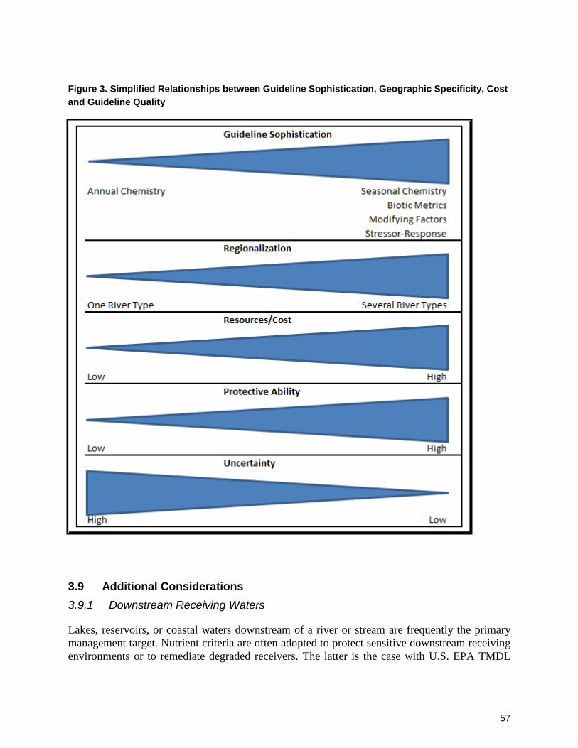
57

Figure 3. Simplified Relationships between Guideline Sophistication, Geographic Specificity, Cost and Guideline Quality

3.9 Additional Considerations 3.9.1 Downstream Receiving Waters

Lakes, reservoirs, or coastal waters downstream of a river or stream are frequently the primary management target. Nutrient criteria are often adopted to protect sensitive downstream receiving environments or to remediate degraded receivers. The latter is the case with U.S. EPA TMDL

58

limits designed to recover impaired waters. Criteria have been used in many areas to achieve specific nutrient targets in receivers, e.g., the Baltic Sea (Helsinki Commission 2007), Chesapeake Bay (U.S. EPA 2010c), and Lake Simcoe (Louis Berger Group and Greenland International, Inc. 2006).

The protection of downstream waters is written into EPA regulation as follows: “EPA's regulations provide that "designating uses of a water body and the appropriate criteria for those uses, the state shall take into consideration the water quality standards of downstream waters and shall ensure that its water quality standards provide for the attainment and maintenance of the water quality standards of downstream waters" (U.S. EPA 2012). For the State of Florida, for example, the implementation of this regulation was described as a two-step process: “The first step is determining the average annual nutrient load that can be delivered to an estuary without impairing designated uses. This is the protective load. The second step is determining nutrient concentrations throughout the network of streams and rivers that discharge into an estuary that, if achieved, are expected to result in nutrient loading to estuaries that do not exceed the protective load. These concentrations, called ‘‘downstream protection values’’ or DPVs, depend on the protective load for the receiving estuary and account for nutrient losses within streams from natural biological processes” (U.S. EPA 2010b). The second step is completed using watershed models.

Figure 4. Steps for Determining “Downstream Protective Values” (from U.S. EPA 2010d)

Nutrient guidelines to protect downstream receivers are derived as loading limits instead of concentrations for use protection, but the loads can be back calculated to derive concentrations. Nutrient guidelines used in this way are not specifically designed to protect aquatic life in the stream or river and can be either more protective (lower) or less protective (higher) than any other guideline applicable to that watercourse. Given that the more protective value applies, however, the downstream consideration only comes into effect if it results in a more restrictive guideline than the guideline to protect in-stream uses.

Total phosphorus guidelines in Manitoba have been differentiated between rivers that flow into a lake or reservoir (0.025 mg/L) and all other streams (0.05 mg/L) (Manitoba Water Stewardship 2011).

59

3.9.2 Seasonality

Many of these guidelines listed in previous sections do not indicate a season in which the guidelines are expected to be met. Lotic systems often show marked seasonal differences in nutrient concentrations especially in those cases where suspended solids are linked to discharge. Considerations with respect to the protection of aquatic life should include seasonal guidelines where appropriate, or be linked to modifying factors such as TSS which are seasonally dependent. Less restrictive seasonal guidelines or objectives (for example for the winter season in comparison with the summer season) can be valid interpretations of a nutrient guideline for specific water bodies, such as demonstrated in the North Saskatchewan River (NSWA 2010) and the Bow River (BRBC 2008).

In many cases nutrient guidelines are linked to plant and algal growth or to oxygen concentrations with the intent of protecting aquatic life during the period of maximum growth or worst case conditions in the environment. The influence of periphyton or rooted aquatic plants on dissolved oxygen in rivers, for example, is greatest during maximum summer growth. Receiving water assessments are frequently calculated for the period of extreme low flow (e.g., the 7Q10 or 7Q20 low flow statistic). Therefore nutrient guidelines may only be required during the open water season, when impacts of nutrient enrichment are strongest. Seasonal variation is often considered during environmental assessments which compare measured data with guidelines to help decide whether or not the measured data are exceeding the guideline. There are, however, no Canadian nutrient guidelines that have been developed to address variations in seasonal conditions in rivers or streams, while some seasonal site-specific objectives have been developed (NSWA 2010, BRBC 2008).

In case where guidelines as developed with the purpose of protecting downstream waters, guidelines should be applicable for the entire year, as the total nutrient load is usually targeted with such a guideline.

3.9.3 Addressing Uncertainties

There are three levels of error that can contribute to the uncertainty surrounding the derivation and use of guidelines:

1. A number of sources of error associated with the data that are used to support the guideline development and that will contribute to uncertainty, including:

• natural, spatial and temporal variability in the data

• sampling error and

• analytical error.

2. Statistical error associated with the relationships between stressor and response variables. Some of this error will be associated with the factors mentioned in 1.

60

3. A degree of error involved in the use of a guideline for one region that has been developed for another region. This uncertainty is difficult to quantify.

These errors contribute collectively to the uncertainty of any derived guideline’s ability to protect the stream or river for designated uses. Ideally, it will be possible to assign error to the results from which the guideline was derived. This is possible in the use of mathematical models or with regression analysis (predictive approaches) but may not be so easy for reference condition approaches where narrative statements or ranges of ecosystem responses are used. In the case of literature values it is often difficult to assess error even when accessing the original literature in which the guidelines were reviewed.

The requirements for the development of guidelines include the need for a method to assess error. For example, the Water Framework Directive (European Union 2000) requires a “sufficient level of confidence about the values for the reference conditions” and “adequate confidence and precision in the classification of the quality elements”, but there is no specific guidance as to what these cautions mean. Some interpretations have been developed (REFCOND 2003).

The U.S. EPA (2010a) provides guidance for evaluating model accuracy and precision when using predictive modeling approaches (Section 5.1, pages 65 – 69).

The weight of evidence approach uses quantified measures of uncertainty to weigh lines of evidence based on the uncertainty that is associated with them. In practice that means that evidence with high uncertainty (or error) receives a low weight and evidence with low uncertainty (error) receives a high weight in the final decision (or, in this case, the final guideline). An example of weighing model results by levels of uncertainty was the development of a eutrophication model for Hamilton Harbor, Ontario. The relative mean standard error was calculated for two available models. Predictions from the different models were then combined using the respective standard error estimates as weights in a weighted model average (Ramin et al. 2012).

All approaches to deriving guidelines should include an estimate of error that is appropriate to the methods used. When the results of multiple approaches are synthesized and used to develop a single guideline, a weight of evidence approach should be used to weigh the results based on the uncertainty associated with them.

4.0 GUIDANCE FOR SETTING NUTRIENT GUIDELINES Section 3 summarized the methods that have been used to derive nutrient guidelines and the resources that are required in each case. This section describes a step-by-step process that includes a closer look at some of the decisions that need to be made with respect to choosing approaches for guideline development. The general step-by-step procedure is shown diagrammatically in two decision trees (Figures 5 and 6).

61

The first decision tree (Figure 5) provides a process for a situation in which a manager has no prior information, or wishes to derive a guideline quickly, in the absence of a detailed understanding or the river or area of concern. Literature values can be used to derive an initial water quality guideline, in which the manager uses their understanding of the river in a geographic and ecoregion context to select a candidate nutrient guideline value from the literature. The guideline value is applied and the manager undertakes a water quality assessment of the area of concern.

• If the river falls outside the guideline and has not resulted in unacceptable ecological impacts then the manager can choose to accept the existing guideline or refine the literature values by additional investigation (Figure 5).

• If the guideline is met but unacceptable ecological changes due to nutrient enrichment are observed, then the guideline needs to be revised.

• If the guideline is met and ecological condition appears unimpaired, the existing guideline can be accepted.

• If the data fall outside the guideline, and unacceptable ecological impacts are observed, the existing guideline can be accepted as well.

As the manager gains understanding of the system and acquires additional information then the guideline can be refined and the literature value replaced with a more sophisticated approach. This is illustrated in Figure 6, as a step-by-step decision tree for the complete guideline development process.

62

Figure 5. Nutrient Guideline Adoption Process – First Application

No Prior Information

Use Simplest Method to Start

Increasing Complexity and Resources Revise Initial Guideline

Not Impaired

Revise Initial Guideline

Refine Guideline as Knowledge

Increases

Test Guideline Applicability

Set Initial Guideline Using Literature Values

Set Initial Guideline Using Literature Values

Investigate Areas of Interest (Nutrient Assessment)

Compare Results to Guideline

Within Guideline

ImpairedImpaired Not Impaired

Exceeds Guideline

Maintain Initial Guideline

Investigate Areas of Interest (Ecological Assessment)

Investigate Areas of Interest (Ecological Assessment)

63

Figure 6. Step-by-step Procedure for Nutrient Guideline Development

64

4.1 Define Geographic Scale It is important to first define the geographic scale that will be served by the nutrient guidelines. This will normally be understood at the point where the need for guidelines is identified. In other words it will be determined beforehand whether the guidelines will be intended for use on a province/territory scale or in a watershed or site-specific setting. Geographic scale will determine both the user and the location in which the guidelines will be applied. “Who requires this guideline?” is therefore a useful first decision that will necessarily include an evaluation of geographic scale. This will dictate differences in both derivation and data requirements.

4.2 Define Desired Outcome The goal of an anticipated guideline needs to be clearly established before any decisions about the “how to” can be made. A nutrient guideline is a tool in nutrient management that serves as a reference point against which the state of the watercourses can be measured. Therefore the desired outcome for the surface waters of the regions of concern needs to be defined before the approach to guideline development will be chosen. For each stream type, the selection of any approaches or methods will depend on the desired outcome. CCME (2003) recommends that the approach to developing guidelines follow the International Joint Commission (IJC) and the Ontario Ministry of the Environment (OMOE), whereby guidelines “are set at such values as to protect all forms of aquatic life and all aspects of life cycles.” Other considerations may include:

• non-degradation, e.g., no deviation from current conditions (for example in protected pristine environments, such as national parks)

• designated use-protection (aesthetics, recreation, aquatic life); the most sensitive use is usually given priority and

• protection of downstream lakes and estuaries – watershed loading approach vs. river protection approach. Occasionally written into guidelines (e.g., Manitoba, and previously Quebec).

The non-degradation principle can either be included in the development of a numeric guideline for specific sites or can be used in the implementation process. Several jurisdictions, for example Manitoba, currently allow that any “sites of exceptional value” that are currently meeting, or are well below, the guideline should not have their water quality degraded further (Manitoba Water Stewardship 2011). In Ontario, where current conditions exceed the applicable guideline (called Policy 2 waters), the non-degradation policy takes effect for any discharge applications and improvement of the conditions is encouraged (OMOE 1994).

The importance of establishing the desired outcome of a guideline cannot be understated. While algal biomass and nutrient concentration usually have a positive relationship, nuisance growth of specific algae can occur at low nutrient concentrations, which would require setting a lower limit, possibly in addition to an upper limit, similar to the pH guideline, which is a range of value. Proliferation of Didymosphenia geminata have been found to occur under very P-limited

65

situations because nuisance accumulations are not a consequence of cell biomass but instead are a result of extracellular polysaccharide stalk material (Bothwell and Kilroy 2011). Such accumulations have been found to not occur when P is supplemented (Kilroy and Bothwell 2012) and indicate the need for a lower nutrient guideline. While this case is likely spatially limited to the areas where Didymosphenia blooms have occurred, it demonstrates the importance of a well-defined desired outcome.

4.2.1 Regional Nutrient Guidelines

Regional guidelines may include entire provinces or territories, individual ecoregions, or large watersheds which are likely the smallest areas that might be considered for a regional guideline. Smaller provinces, such as Prince Edward Island, may be considered for one regional guideline, given that it is only one ecoregion. The large provinces and territories in Canada encompass several ecoregions and therefore should consider subdivision into ecoregions or another classification that takes climatic and landscape variation into account.

Within Canada there are ecoregion guidelines that have been developed in Alberta (Janna Casson, Alberta Agriculture and Rural Development, personal communication) and for several agricultural regions across Canada by the NAESI (National Agricultural Environmental Standards Initiative, Chambers et al. 2009). There are guidelines developed for smaller, unique, and isolated areas such as Vancouver Island. Watershed plans have been developed or are being considered for large and nutrient enriched watersheds such as the Grand River or Lake Simcoe in Ontario. These smaller geographic scales could be considered as being site-specific since they are focusing on a single river or receiver.

4.2.2 Site-Specific Nutrient Guidelines

Site-specific guidelines are developed where there is concern that any regional guidelines that are in place are not adequate or where regional guidelines do not exist. Site-specific guidelines may apply to smaller streams, rivers, or reaches within a river. The reports presenting the only site-specific nutrient guidelines developed so far in Canada provide the following rationale:

“Site-specific water quality guidelines are prepared for specific bodies of fresh, estuarine and coastal marine surface waters of British Columbia and the Yukon as part of Environment Canada’s mandate to report on water quality. Site-specific guidelines (SSGs) are prepared to protect all designated water uses. The site-specific water quality guidelines proposed in this report differ from the traditional water quality objectives in that they are meant for the purpose of reporting on water quality relative to only one water use – protection of aquatic life.” (Tristar Environmental Consulting 2005b)

Essentially, these site-specific guidelines are interpretations of generic guidelines for the circumstances observed at a specific site in a specific river for the purpose of national reporting, but had no other management consequences associated with them. This is in contrast to site-specific objectives developed for several Alberta rivers, which were developed using similar methods, but are tied to management commitments.

66

Golder (2005), in a review of site-specific guideline methodologies, defined a site-specific guideline as: “a numerical concentration or narrative statement based on science recommended to support and maintain the protection of aquatic life based on conditions at a specific site.” This definition could apply equally well to guidelines for toxicants or nutrients. Examples of site-specific guidelines for nutrients in Canada include:

• Skeena, Kootenay, Sumas, Liard Rivers, BC (Tristar Environmental Consulting 2005a,b,c,d).

Examples for site-specific objectives developed for nutrients in Canada include:

• North Saskatchewan River (NSWA 2010, MacDonald 2013)Bow River (Bow River Basin Council (BRBC) 2008).

4.3 Select Guideline Variables The suitability of any variable will depend on its relevance for the desired outcomes for the regulated ecosystem. The outcomes themselves may also differ between systems. For example, some researchers have developed guidelines for periphyton biomass in streams (New Zealand guideline: Biggs et al. 2000a) whereas others have focused on sestonic biomass (large rivers, Minnesota: Heiskary et al. 2010). In some cases macroinvertebrate or fish metrics may be more suitable, especially in naturally enriched systems where further nutrient additions will have less impact on periphyton. This may also be the case in systems with unsuitable substrate types or too much turbidity for periphyton to be used as a suitable response variable.

The suitability of different algal indicators for different levels of pressure was demonstrated by Kelly et al. (2009). Autotrophic metrics were particularly responsive at low levels of nutrient (organic) pressure while heterotrophic metrics were more responsive at higher pressure levels. For nutrient guidelines this means that in regions of naturally high nutrient levels, such as in the prairies, indices based on macroinvertebrates or fish may perform best while in regions with naturally low nutrient levels algae indicators possibly perform best.

In all cases, it is important to determine whether the guideline should be based entirely on the stressor variable, e.g., TP and TN, or whether the guideline could be better expressed as a response variable. When a strong stressor-response relationship is confirmed, stressor variables are suitable for nutrient guidelines. When modifying factors have a dominating effect on the aquatic productivity of a stream, a guideline based on periphyton biomass may be more effective (Kistritz and MacDonald 1990).

The Maine Department of Environmental Protection (2012) offers the possibility to use the Diatom Total Phosphorus Index (DTPI) and Diatom Total Nitrogen Index (DTNI) as a surrogate measure (instead of TP). Phosphorus and at least one response variable (percent algal cover, water column chl “a”, Secchi disk depth, DO, patches of bacteria and fungi, aquatic life) have to exceed guideline values at a site to lead to an “impaired” classification. This leaves the option open to develop site-specific TP guidelines where there is no biological effect detected at TP concentrations which are exceeding the guideline.

67

Often the guideline variables that should be used will be determined through the examination of stressor-response relationships (using the predictive modeling approach; see section 3.4). The choice of a variable for the guideline would be the nutrient fraction that best explains responses in the measured biotic communities. If that approach is used, only the response variable(s) should be selected at the initial variable selection stage and all potential stressor variables related to nutrient dynamics should be considered in the data collection and analysis to determine the most suitable one(s) for guideline development.

One example for a stressor-response relationship used to select the most appropriate variable for site-specific nutrient objectives are the reach-specific phosphorus objectives for the Bow River in Alberta. The management goal of a healthy ecosystem included the desire to assure oxygen conditions supporting certain fish populations in specific reaches of the river. The total and dissolved phosphorus concentrations required to sustain those oxygen conditions were modeled (BRBC 2008). As a result, TP and TDP objectives were developed for some reaches and TDP objectives only for others, depending on the observed predictive relationships between nutrients, algal biomass and oxygen.

A group of European scientists, convened to develop standardized implementation protocols for the reference condition approach, have defined criteria for indicator selection (REFCOND, 2003). Indicators, in this case, are metrics that describe the biotic response variables, and the selection of indicators was described as an iterative process, requiring consideration of many factors, as described below:

• Relevance: An indicator should describe the condition of the biological organism group. It should be capable of indicating the response of the biota to pressures.

• Responsiveness: Indicators should be sensitive to one or more of the stressors of interest, in this case, nutrients.

• Range of sensitivity: Indicators should show effects over a range of pressures but reach their maximum response at a low level of pressure (e.g., a sensitive species may disappear). It may be necessary to use multiple indicators.

• Ability to estimate reference values: Where there are no sites at reference condition, other options may be to borrow sites from neighbour regions or states, use historical data, modelling or expert judgement to estimate reference conditions for some indicators.

• Variability: Indicators whose natural variability is high and poorly understood are likely to be unsuitable.

• Confidence: Indicators should be selected so that there is good and demonstrable confidence and precision in classification of ecological status.

• Risk of misclassification: If risk is too large, more than one indicator may be used to estimate the condition of the biota. In such cases, the number of indicators, and the means by which the

68

data for these are combined, should be such as to achieve the required degree of confidence in the estimate for the biotic variable.

Another important factor to consider is feasibility. A guideline variable has to be measurable in a consistent way and by a wide variety of organizations that conduct water quality monitoring. While biological indicators are the most direct estimates of ecosystem health, the data collection and analysis effort is higher than for TP or TN measurements on water samples. Unless there is the commitment or existing capacity (such as periphyton monitoring in some Alberta rivers or macroinvertebrate monitoring in Ontario) to implement biological monitoring across the jurisdiction of interest, phosphorus and nitrogen guidelines are currently the most easily implemented nutrient guidelines.

Many of the above considerations reinforce the need to explore multiple lines of evidence when setting guidelines. This will include the use of multiple variables in those cases where this approach will reduce uncertainty in the end use of the guideline.

When considering the development of guidelines for either nitrogen or phosphorus or both, it may be useful to look to the neighbouring U.S. states that have recently gone through the process of developing nutrient guidelines. The U.S. EPA guidance recommends addressing both nitrogen and phosphorus in guideline development, but some states only developed phosphorus guidelines, some only nitrogen guidelines, and many have developed guidelines for both (Figure 7).

69

Figure 7. Progress of Nutrient Guideline Development in U.S. States by February 2013.

Note: This map was obtained from the U.S. EPA website http://www.epa.gov/nandppolicy/progress.html.

4.4 Classify Streams

4.4.1 Is Stream Classification Required?

For the development of regional nutrient guidelines, stream classification may be appropriate in most cases, but in other cases it might not be required. The larger and more diverse the region of interest is in terms of natural subregions, the higher the likelihood that classification is useful. For site-specific guidelines, the region of interest may be too small to justify classification.

The need for stream classification should be determined by the presence of any regional (geology, soils, climate) or local (site-specific, size, substrate, flood frequency) modifying factors that vary significantly within the region of interest. The examination of ecoregional, geological and soil maps, and knowledge of stream sizes and substrate types will help classify streams. If significant differences are suspected, a stream classification should be attempted.

70

4.4.2 Classification Procedure

4.4.2.1 Determine Applicability of Existing Classification Schemes

The existing classification schemes or their modifications can be well suited to stream classification in the region of interest. The applicability of existing Canadian or U.S. ecoregion classifications (section 3.2.1) should be explored first as that is the least costly and most straight-forward classification method. The analysis of available data on nutrient concentrations and biota for significant differences among regions is one way to assess if existing classification schemes are appropriate for nutrient guideline development.

There are several circumstances, however, that may warrant the development of a “custom” or regional stream classification for an area of interest. These include situations where:

1) regional factors other than those accounted for in ecoregions are important for nutrient dynamics in the area

2) the selected biological response variable shows stronger relationships with local modifying factors than with regional factors or

3) the number of ecoregions cannot be sufficiently covered with monitoring data.

All these situations can be identified through a preliminary analysis of existing data or may only become evident from the analysis of data collected for the intent of guideline development. Experience in U.S. states has shown that it is useful to establish one or more draft stream classifications at the start of guideline development and to assess which one of the classification systems is most appropriate during the data analysis. For example, for the development of Wisconsin nutrient guidelines, both the EPA nutrient regions and the nutrient zones developed by Robertson et al. (2001) were considered (see section 3.2.1) and carried through the data analysis. In the end, a modified and simpler version of the nutrient zones was adopted (Figure 8), as it best explained differences in nutrients and biota among wadeable streams in the State of Wisconsin (Robertson et al. 2006).

71

Figure 8. Process of Regionalization for Nutrient Criteria in Wisconsin (Robertson et al. 2006)

Considered Draft Regionalization Schemes

Final Proposed Regionalization Following Data Analysis

72

4.4.2.2 Develop New Classification

If existing classification systems are deemed inappropriate, a new classification system can be developed based on known or suspected modifying factors and/or classification variables described in section 3.2.2. Modifying factors acting on regional scales (section 4.4.2.1) are of interest for classification schemes supporting the development of regional guidelines. Local modifying factors (section 1.4.2.2) can be used to refine a regional classification scheme, to classify reaches of one river or stream or for the development of site-specific guidelines. All modifying factors that are known to vary across the region of interest should be considered for stream classification, although it may not be practical to use them all in the final classification scheme. A number of variable combinations that have previously been used to classify streams can be considered for application (section 3.2.2).

The classification method (section 3.2.3) should be chosen to analyze the data and group streams into different types on the basis of the selected variables. The development of a new classification system will require geospatial data, nutrient data and biological data, if available. The analysis will benefit from GIS expertise and requires staff resources for data analysis. Developing a new classification scheme is therefore most likely to require more data and resources than adopting an existing classification scheme.

4.5 Evaluate and Select Approaches If a “multiple lines of evidence” approach is attempted, as described in this manual, all three available approaches should be evaluated and the preferred or most applicable options selected. The availability of data and resources should be evaluated when reviewing the approaches and methods available. Previously completed studies and monitoring data should be integrated into the guideline development process where possible to build upon regional experience and wisely use resources. Previous studies can provide information about stressor-response relationships, regional differences and sensitive biota that may be useful as a response variable.

Among the three approaches, the predictive modeling approach could be viewed as the most scientifically rigorous, as it depends the least on professional judgement and the most on empirical data.

The reference condition approach can be scientifically rigorous when based on well-rounded knowledge about ecological requirements of biological communities, an understanding of and presence of reference conditions in the area of interest and solid statistical approaches to detect significant deviations from reference conditions.

The percentile method used to identify reference conditions and develop guidelines based on data distributions lacks the linkage to biotic response variables and is therefore associated with a high degree of uncertainty. It is easy to calculate, however, and not costly if representative datasets are already available, and therefore has traditionally been included in many nutrient guideline studies.

73

Finally, existing guidelines can be used if they are deemed applicable for the region of interest. They have the advantage of minimal required effort and cost.

In the following sections, we provide more detailed considerations that should help evaluating the applicability of approaches and assist in selecting the most appropriate methods within the three types of approaches for guideline development. The levels of resources associated with using each particular method are discussed in section 0.

4.5.1 Reference Condition Approach

4.5.1.1 Applicability

The reference condition approach is applicable if:

1) Reference sites are available for the identified stream types. If there are reference sites for only part of the stream types, reference conditions for the missing types can be either inferred (sections 3.4.2.2) or other approaches (predictive modeling, literature values) can be used to obtain guidelines for stream types without reference sites.

2) There are not enough data or resources to describe and use stressor-response relationships using the predictive modeling approach.

The reference condition approach has limited applicability if:

1) No reference sites are available for the stream types (reference conditions cannot be measured and must be inferred).

2) A site-specific guideline is desired (site-specific reference conditions must rely on historical data, which are often lacking or of limited quality).

4.5.1.2 Involved Steps

Use of the reference condition approach involves the identification of reference sites (Section 3.4.1), the description of reference conditions (section 3.4.2 and the determination of an acceptable departure from the reference condition, which then becomes the guideline (Section 3.4.3).

4.5.1.3 Evaluation and Selection of Methods

The choice of methods for the reference condition approach depends largely on two conditions: first, on the number and proportion of reference sites compared to the overall number of water bodies, and second, if resources are available to conduct a biological reference condition study. If no reference sites are available, reference conditions have to be modeled or estimated using the lower percentile approach. If reference sites are available in suitable numbers, upper percentile methods, midpoint analysis on nutrient data or biological approaches can be used, which provide

74

an increasing level of confidence in the guideline values. While biological approaches are the most costly, previous work can be reutilized where available to limit additional cost.

4.5.2 Predictive Modeling

4.5.2.1 Applicability

There are several situations that lend themselves to the consideration of the predictive modeling approach:

1) If data exist (academic, government work) that demonstrate or indicate strong stressor-response relationships. In this case, one can choose to:

a. use this work to develop guideline without further work

b. re-analyze existing data using more advanced statistical methods and/or

c. add new data to refine relationships.

2) If strong stressor-response relationships are expected based on expert judgement:

a. a pilot study may be initiated to verify this expectation

b. if a pilot study confirms the relationship or if there is high confidence in the presence of a relationship, collect a larger data set to support guideline development.

3) If whole river models are already set up (e.g., Bow River, Golder 2007) or local modeling capacities exist.

4) If the Reference Condition Approach has been determined as not applicable or not feasible.

4.5.2.2 Involved Steps

The general steps involved with the predictive modeling approach are the identification of relationships (section 3.5.1), the examination of relationships (section 3.5.2) and the establishment of thresholds and/or criteria (section 3.5.3).

4.5.2.3 Evaluation and Selection of Methods

The selection of methods for predictive modeling is mainly dictated by the type of available data. Generally, if water chemistry and physico-chemical data as well as univariate biological data (e.g., periphyton biomass) are available, correlation and regression techniques are the most applicable to develop predictive models of nutrient enrichment. Within these techniques, care has to be taken to assess the data distributions for all analyzed variables (i.e., normal versus non-

75

normal) and the shape of relationships (linear versus non-linear) in order to select the most appropriate and powerful method for the data analysis.

If multivariate response variables are analyzed, such as biological community data or multiple biological metrics, multivariate methods, such as ordination, are more appropriate methods to use. For biological data the suggestion is to explore data distribution and shapes of relationships first in order to select the most appropriate methods (linear versus unimodal or other response models).

4.5.3 Literature Values

Use of literature values, such as existing guidelines, should always be included in guideline development, because it:

1) requires little time and resources

2) adds one piece of evidence and credibility if well researched

3) can make use of the large amount of work done in neighbouring U.S. states and other jurisdictions.

Literature values are a good starting point for the derivation of guidelines when no other information is available. The guideline can be set and then studies initiated to determine its applicability or the need to develop guidelines by more intensive methods. The most important consideration when using literature values is to assess their applicability to the region or site of interest.

4.5.3.1 Applicability

The following criteria should be considered, at a minimum to assess the applicability of available literature values:

1) Regional modifying factors (climate, geology, soils, see section 1.4.2.1)

2) Local modifying factors (flow and substrate, see section 1.4.2.2)

3) Distance, due to biogeographical considerations if the guideline is based on biotic communities (check if the applied algal, benthic invertebrate or fish metrics are applicable to the geographic area of interest).

If all or most of these factors are comparable between the area where the literature value was derived and the area for which a guideline is being developed, then the literature value is a good candidate to use in the multiple lines of evidence approach.

76

4.6 Collect and Analyze Data The process of collecting and analyzing data to support guideline development will be different than the monitoring and analysing that will occur to establish whether or not guidelines are being met (post guideline development). For example the reference conditions approach and predictive modelling approach require a rigorous study design that includes a monitoring program tailored to the needs of the tested hypotheses and planned statistical analyses. The monitoring program may also have to be adapted to unexpected conditions, such as high variability in the monitored variables or a new modifying factor that becomes obvious.

There are many references to describe various aspects of study design, sample collection and data analysis, including recommendations with respect to which statistical methods to use (U.S. EPA 2010a). Generally:

• if the reference approach is used it will be necessary to evaluate the suitability of reference location samples and assess how best to develop guidelines relative to these data

• if predictive modelling is used there will be many inputs to these models that will need to be determined through empirical data collection or through the development of assumptions

• the use of literature values or guidelines developed elsewhere will not normally require the collection or analysis of data.

With any approach where guidelines are being derived through the collection and analysis of data it will be important to consider seasonality, i.e. whether the designated uses, stressor and response indicators or the analyzed stressor-response relationships vary among seasons. It may be necessary to identify those time periods of the year when the guideline is valid. It makes sense, for example, to limit sampling to the open-water season when guidelines are to be developed based on relationships between nutrients and benthic algae and macroinvertebrates or, if percentiles are used, to develop guidelines for different seasons or flow seasons.

The length of record required to develop guidelines depends on the chosen method. When percentiles are used to describe the current population of sites, one representative average (or median) value per site is used to calculate that percentile. For this value to be representative of the site, data from a number of years are needed. At the very minimum, two years of data, but preferably three or more are recommended (U.S. EPA 2000). If funds are limited, restricting sampling frequency within each year and/or numbers of constituents analyzed should be considered to preserve a longer-term data set. In most jurisdictions, existing monitoring datasets can be used to calculate percentiles of reference streams and rivers or of the entire stream dataset. The U.S. EPA recommends a minimum total number of 30 streams and a minimum of three low-impact reference systems per stream type or ecoregion for developing nutrient criteria based on the percentile approach.

Bi-weekly (every two weeks) to monthly sampling throughout the growing season for multiple years is required for the study of stressor-response relationships between nutrients and biota and

77

to determine peak algal biomass and potential thresholds (U.S. EPA 2000). Two or more years of data are required to identify inter-annual ranges of climate or flow. The higher the flow variations are in a river system, the more sampling visits are required (U.S. EPA 2000).

The types of data analyses associated with each approach have been described in previous sections. The end result will be a set of draft guidelines (Chambers et al. (2009) used the term “provisional”) that will then need to be evaluated (See section 4.7 below).

4.7 Assess Level of Uncertainty If the results provide predictive ability and limited uncertainties, they can be used in the next step to establish the final guidelines. If they are not, the reasons for low predictive ability should be investigated:

• If stressor-response relationships vary spatially, the stream classification may have to be revised.

• If the influence of confounding factors is too large, it may be useful to include them in the guideline formulation (e.g., TSS-TP correlation).

If the method or approach still does not reveal useful results, it may have to be omitted from the guideline development. If more evidence is required for the weight of evidence approach, an alternative method or approach should be selected, or additional lines of evidence should be obtained, which together will reduce uncertainty to an acceptable level.

4.8 Establish Guideline(s) When all draft guidelines resulting from different approaches and the levels of uncertainties associated with them have been completed, the final nutrient guideline or guidelines can be developed. If estimates of uncertainty are available, the draft guidelines should be weighed according to the level of uncertainty associated with them to determine the final guideline.

Final guidelines should be used with the knowledge that there will always be new findings that may further endorse, or indicate limited value to, their continued use. The effects of climate change or the impacts of multiple stressors, for example, may limit the applicability of nutrient guidelines and knowledge in these areas is rapidly evolving. Regular reassessment of established nutrient guidelines, and if necessary, revisions to the guidelines are therefore recommended.

5.0 SUMMARY Eutrophication is one of the major water quality issues in Canadian waters. Existing Canadian Water Quality Guidelines mainly address toxic effects and not the effects of nutrient enrichment on aquatic biota. Nutrient guidelines are used in several Canadian jurisdictions, but they often do

78

not take into account the large natural variations in nutrients across different natural regions or modifying factors that affect the translation of nutrient concentrations into biological responses.

This guidance manual provides methods and supporting information to facilitate the development of nutrient guidelines for streams and rivers across Canada that are scientifically defensible and that take into account the natural diversity of watercourses.

A comprehensive review of the literature was conducted to assemble information on the existing approaches and methods that are used in nutrient guideline development in Canada and other countries. The review consulted the large volume of literature produced through recent efforts to standardize guideline development in other jurisdictions (U.S., Europe, Australia and New Zealand) and the supporting scientific literature on nutrient indicators, nutrient-biota relationships and stream classification systems.

The literature review revealed that there are three general approaches available for guideline development: the reference condition approach, predictive models, and the adoption of applicable guidelines from other jurisdictions or literature values. Each of these approaches can be implemented using a broad range of indicators and methods, the choice of which depends on the availability of existing data, the access to resources and on the natural characteristics of the region of interest.

The general process of guideline development consists of a number of consecutive steps and associated considerations, which are listed and discussed briefly below.

1. Definition of the area of interest and with that the decision if a regional or site-specific guideline is required

• regional guidelines may include provinces, territories, ecoregions or large watersheds

• site-specific guidelines are developed where there is concern that regional guidelines are not adequate and may apply to smaller streams, rivers, reaches within a river or a specific site.

2. Establishment of the desired outcomes, which

• may include the protection of designated uses

• can include non-degradation principles and protection of downstream water bodies

• must be defined clearly and accommodate specifics of the region.

79

3. Selection of the guideline variable(s)

• for the Canadian context this manual uses the terminology of chemical stressor and primary and secondary response variables plus the concept of modifying factors

• chemical stressor variables, such as TP and TN, are the most commonly used variable

• it is desirable to confirm the most appropriate stressor variables through a study of stressor-response relationships, but feasibility in terms of continued monitoring has to be considered as well

• primary response variables, such as periphyton biomass, may be more effective for protecting the targeted uses and level of ecosystem health, in particular when stressor-response relationships are poorly understood

• developing guidelines for multiple variables may increase flexibility and reduce uncertainty in guideline application.

4. Classification of streams or subdivision of the area of interest into regions

• stream classification may not be required in small and homogenous areas, while in large areas with a variety of natural regions, guideline development will benefit from stream classification

• the presence of any regional (geology, soils, climate) or local (size, substrate, flood frequency) modifying factors that vary across the area of interest indicate the need for stream classification

• if a need for stream classification is confirmed, existing classification schemes, such as Canadian or U.S. ecozones, ecoregions and ecodistricts or any combination of these are the simplest way to subdivide the area of interest

• if existing classification systems are deemed inappropriate, a new classification system can be developed based on known landscape and/or stream characteristics.

5. Evaluation and selection of methods

• literature values, such as existing guidelines and threshold values should always be included in guideline development, because it is cost effective, can be highly relevant and makes use of existing knowledge

• the percentile method as the simplest form of the reference condition approach provides an simple and cost-effective way to make use of existing data in the area of interest, but lacks the linkage to biotic response variables and therefore is associated with a high degree of uncertainty

80

• the reference condition approach can be scientifically rigorous when a sufficient number of reference sites is available and well identified, ideally using biological communities, but can be cost-intensive as it requires a good spatial coverage of the area of interest and biological data collection and analysis

• predictive modelling could be viewed as the most rigorous approach, as it depends most on empirical data on stressor-response relationships but requires chemical and biological data and advanced technical expertise.

6. Collection and analysis of data

• for the adoption of literature values, no further data collection and analysis is required, as it only involves a literature review and assessment of applicability based on existing information

• when using the percentile approach, data from three or more years per site are required and a minimum total number of 30 stream and at least three reference sites are recommended per stream type

• for the study of stressor-response relationships bi-weekly (every two weeks) to monthly sampling throughout the growing season for multiple years is recommended

• the reference condition approach requires that the spatial and temporal variability in the reference sites is well understood and therefore involves a significant sampling effort, which may be cost-intensive, as reference sites may be located in remote areas

• the monitoring program needs to be tailored to the adopted study approach such that the resulting data are suitable to the required statistical analyses and may need to be adapted if the monitored variables show higher variation than expected or if new modifying factors are identified.

7. Assess the Level of Uncertainty

• predictive ability of the stressor-response relationships or levels of variation in results provide a measure of uncertainty around the guideline value

• spatial variation may be addressed by revising stream classification and influence of confounding factors can be included in guideline development.

8. Establishment of guidelines

• the use of multiple lines of evidence is suggested, i.e., a number of draft guideline values resulting from different approaches should be used as input for the establishment of the final guideline value

81

• seasonality should be explicitly addressed in guideline formulation where appropriate, as nutrient effects usually vary considerably among seasons

• the level of uncertainty associated with each approach should be used in a “weight of evidence” approach, where possible, i.e., results with low uncertainty should receive a larger weight in the final guideline than results with high uncertainty.

Region- and jurisdiction-specific considerations play a crucial role in each of these steps. There is no ideal “one-fits-all” approach to nutrient guideline development, because each region and jurisdiction has a unique combination of natural features, economic and intellectual resources, and existing data monitoring programs.

Developing a nutrient guideline is not a one-time, straight-forward undertaking. In some cases the initial decisions, such as variable choice and stream classification scheme, have to be revised as a result of method evaluation in terms of feasibility and in response to data analysis results. Generic initial guidelines may have to be verified for their applicability and refined over time.

Regions faced with limited resources or when a draft guideline is a desired first step, a more simple procedure may be more appropriate as an alternative to the complete guideline process outlined above. This procedure consists of the adaptation of a literature value as an interim guideline and then the iterative refinement of the guideline as more ecological data from the rivers become available.

Cost of nutrient guideline development depends on a variety of factors. In general, costs increase with guideline sophistication in terms of methods and the number of variables and seasons considered, as well as the inclusion of stream classification. Available data and technical expertise as well as partnerships can reduce cost. The use of literature values and the percentile approach are cost-effective, but result in a higher level of uncertainty and therefore potentially lower protection of the aquatic ecosystem.

This guidance manual summarizes a large number and diversity of variables, approaches and methods applicable to nutrient guideline development and provides guidance on how these tools can be used in the process of guideline development. The manual can thereby support the further development of scientifically defensible and regionally and locally relevant nutrient guidelines across Canada.

82

6.0 GLOSSARY TERM DEFINITION REFERENCE FOUND IN algal biomass The weight of living algal material in a unit area at a given time Wetzel 1983 N-Steps website

ash-free dry weight

An algal biomass measurement that measures the standing crop of algae to estimate net production APHA 2000 N-Steps website

Bayesian Analysis

Bayesian Analysis uses the Bayes theorem, which is a formula for revising a priori probabilities after receiving new information. The method has been used in stream classification to find combinations of classification variables that best account for observed variability.

Lamon and Qian 2008; statistics.com

USEPA 2010

benthos/benthic The assemblage of organisms associated with the bottom, or the solid-liquid interface of the aquatic system. Generally applied to organisms in the substrata Wetzel 1983 N-Steps website

biological integrity The ability of an aquatic ecosystem to support and maintain a balanced, adaptive community of organisms having a species composition, diversity, and functional organization comparable to that of natural habitats within a region.

N-Steps website N-Steps website

community all the groups of organisms living together in the same area, usually interacting or depending on each other for existence N-Steps website N-Steps website

criteria

Elements of jurisdictional water quality standards, expressed as constituent concentrations, levels, or narrative statements, representing a quality of water that supports a particular use. When criteria are met, water quality will generally protect the designated use.

USEPA 1994 USEPA 2000

designated uses Uses defined in water quality standards/objectives for each water body or segment whether or not the use is being attained. USEPA 1994 USEPA 2000

Ecodistrict An Ecodistrict is a subdivision of an ecoregion which is characterized by a distinctive assemblage of relief, landforms, geology, soil, vegetation, water bodies and fauna. Canada is divided into 1024 Ecodistricts.

Marshal and Schut 1999

Environment Canada 2006

ecological threshold

The point at which there is an abrupt change in an ecosystem quality, property or phenomenon, or where small changes in an environmental driver produce large responses in the ecosystem.

Groffman et al. 2006

Groffman et al. 2006

Ecoprovince A subdivision of an ecozone is characterized by major assemblages of structural or surface forms, faunal realms, and vegetation, hydrology, soil, and macro climate. Canada is divided into 53 ecoprovinces.

Marshal and Schut 1999

Environment Canada 2006

83

TERM DEFINITION REFERENCE FOUND IN ecology “Ecology is the scientific study of the processes influencing the distribution and

abundance of organisms, the interactions among organisms, and the interactions between organisms and the transformation and flux of energy and matter.”

Likens 1992 Likens 1992

Ecoregion An ecoregion is a subdivision of an ecoprovince and is characterized by distinctive regional ecological factors, including climate, physiography, vegetation, soil, water, and fauna. Canada is divided into 194 ecoregions.

Marshal and Schut 1999

Environment Canada 2006

Ecozone

Ecozones define the ecological mosaic of Canada on a sub-continental scale. They represent an area of the earth’s surface representative of large and very generalized ecological units characterized by interactive and adjusting abiotic and biotic factors. Canada is divided into 15 terrestrial ecozones.

Marshal and Schut 1999

Environment Canada 2006

eutrophic Abundant in nutrients and having high rates of productivity frequently resulting in oxygen depletion below the surface layer. Wetzel 1983 N-Steps website

eutrophication Eutrophication refers to natural or artificial addition of nutrients to bodies of water and to the effects of the added nutrients.

National Academy of Science 1969.

USGS website. http://toxics.usgs.gov/definitions/eutro

phication.html

Guideline (French: Critères de qualité de l'eau)

A numerical concentration or narrative statement recommended to support and maintain a designated water use. Guidelines are upper limits (and lower limits for some parameters such as dissolved oxygen and pH) intended to protect water uses from human‐caused changes to water quality. They provide consistent, science‐based benchmarks for protection at national, regional or provincial scale but do not consider site‐specific, local factors and conditions.

AENV 2012, CCME 1999 NSWA 2010

habitat a place where the physical and biological elements of ecosystems provide a suitable environment including the food, cover, and space resources needed for plant and animal livelihood.

N-Steps website N-Steps website

84

TERM DEFINITION REFERENCE FOUND IN

hydrology The study of the distribution, properties, and effects of water on the earth's surface, in the soil and underlying rocks, and in the atmosphere.

U.S. Environmental Protection Agency (1997) Terms of Environment: Glossary, Abbreviations and Acronyms.

http://iaspub.epa.gov/sor_internet/registry/termreg/searchandretrieve/termsandacronyms/search.

do

lentic Relatively still-water environment Goldman and Horne 1983 N-Steps website

lotic Running-water environment Goldman and Horne 1983 N-Steps website

macroinvertebrate Small benthic organisms which are retained on sieves with a mesh size >2 mm Thorp and Covich 1991 N-Steps website

macrophyte (also known as SAV-Submerged Aquatic Vegetation) Larger aquatic plants, as distinct from the microscopic plants, including aquatic mosses, liverworts, angiosperms, ferns, and larger algae as well as vascular plants; no precise taxonomic meaning

Goldman and Horne 1984 N-Steps website

mesotrophic Having a nutrient concentration that results in moderate productivity Wetzel 1983 N-Steps website

metric

A calculated term or enumeration representing some aspect of biological assemblage, function, or other measurable aspect and is a characteristic of the biota that changes in some predictable way with increased human influence. A multimetric approach involves combinations of metrics to provide an integrative assessment of the status of aquatic resources.

N-Steps website N-Steps website

multivariate community analyses

Statistical methods (e.g., ordination or discriminant analysis) for analyzing physical and biological community data using multiple variables. N-Steps website N-Steps website

85

TERM DEFINITION REFERENCE FOUND IN

non-degradation policy

An environmental policy which disallows any lowering of naturally occurring quality regardless of pre-established health standards.

U.S. Environmental Protection Agency (1997) Terms of Environment: Glossary, Abbreviations and Acronyms.

http://iaspub.epa.gov/sor_internet/registry/termreg/searchandretrieve/termsandacronyms/search.

do

objective A numerical concentration or narrative statement which has been established for specific waters, and which has an action and/or management commitment.

AENV 2012, CCME 1999 AENV 2012

oligotrophic Trophic status of a waterbody characterized by a small supply of nutrients, low production of organic matter, low rates of decomposition. after Wetzel 1983 N-Steps website

outcomes For planning purposes, "outcomes" are the desired endpoints that should guide the development and implementation of the recommendations.

BRBC 2008 - TC report to SC

BRBC 2008 - TC report to SC

parameter see "Variable"

periphyton Associated aquatic organisms attached or clinging to stems and leaves of rooted plants or other surfaces projecting above the bottom of a water body, rocks (epilithic), sediment (epipelic), sand (episammic), plants (epiphytic) or animals (epizoic)..

USEPA 1994 N-Steps website

point source Origin of a pollutant discharge from a discrete conveyance typically thought of as an effluent from the end of a pipe. N-Steps website N-Steps website

primary production

Quantity of new organic matter created by photosynthesis or chemosynthesis, or stored energy which that material represents. Primary production in rivers and streams is usually dominated by algal and macrophyte production.

after Wetzel 1983 N-Steps website

propensity score A composite variable that combines all covariates in a stressor-response relationship into one. When used in the classification of water bodies, they minimize the effect of covariates on stressor-response relationships within each class.

U.S. EPA 2010 U.S. EPA 2010

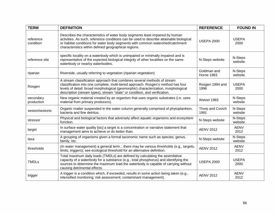
86

TERM DEFINITION REFERENCE FOUND IN

reference condition

Describes the characteristics of water body segments least impaired by human activities. As such, reference conditions can be used to describe attainable biological or habitat conditions for water body segments with common watershed/catchment characteristics within defined geographical regions.

USEPA 2000 USEPA 2000

reference site specific locality on a waterbody which is unimpaired or minimally impaired and is representative of the expected biological integrity of other localities on the same waterbody or nearby waterbodies.

N-Steps website N-Steps website

riparian Riverside, usually referring to vegetation (riparian vegetation) Goldman and Horne 1983

N-Steps website

Rosgen

A stream classification approach that combines several methods of stream classification into one complete, multi-tiered approach. Rosgen’s method has four levels of detail: broad morphological (geomorphic) characterization, morphological description (stream types), stream “state” or condition, and verification.

Rosgen 1994 and 1996

USEPA 2000

secondary production

New organic material created by an organism that uses organic substrates (i.e. uses material from primary producers). Wetzel 1983 N-Steps

website

seston/sestonic Organic matter suspended in the water column generally comprised of phytoplankton, bacteria and fine detritus.

Thorp and Covich 1991

N-Steps website

stressor Physical and biological factors that adversely affect aquatic organisms and ecosystem function. N-Steps website N-Steps

website

target In surface water quality [sic] a target is a concentration or narrative statement that management aims to achieve or do better than. AENV 2012 AENV

2012

taxa A grouping of organisms given a formal taxonomic name such as species, genus, family, etc. N-Steps website N-Steps

website

thresholds (In water management) a general term…there may be various thresholds (e.g., targets, limits, triggers); see ecological threshold for an alternative definition. AENV 2012 AENV

2012

TMDLs

Total maximum daily loads (TMDLs) are defined by calculating the assimilative capacity of a waterbody for a substance (e.g., total phosphorus) and identifying the sources to determine the maximum load the waterbody is capable of carrying without causing detrimental effects.

USEPA 2000 USEPA 2000

trigger A trigger is a condition which, if exceeded, results in some action being taken (e.g., intensified monitoring; risk assessment; contaminant management). AENV 2012 AENV

2012

87

TERM DEFINITION REFERENCE FOUND IN trophic state The production rate of autotrophic or heterotrophic processes in an ecosystem. Dodds 2007 Dodds

2007

variable a substance in, or condition of, the water. Sometimes referred to as a parameter. It may be physical, chemical, biotic or radiological. AENV 2012 AENV

2012

water quality guideline See "guideline" CCME 1996 BRBC

2008

water quality objective See "objective" CCME 1996 BRBC

2008

watershed The area of land that drains water, sediment, and dissolved materials to a common outlet at some point along a stream channel. In American usage, watershed is synonymous with the terms drainage basin and catchment.

Dunne and Leopold 1978

N-Steps website

88

7.0 REFERENCES

This reference list has been categorized into various topics discussed in the guidance manual (see Table 3), including the identification of references pertaining to lakes(i).

(c) Alberta Environment. 1999. Surface Water Quality Guidelines For Use In Alberta. Environmental Assurance Division, Science Standards Branch. November 1999.

(b) Alberta Environment and Water (AEW). 2012. Guidance for deriving site-specific water quality objectives for Alberta rivers. Ver. 1.0 Water Policy Branch, Policy Division. Edmonton.

(q) APHA 1995. American Public Health Association Standard Methods for the Examination of Water and Wastewater 19th ed. Washington, DC.

(q) Atlas of Canada 2012. Canada: Terrestrial Ecoregions 1993. http://atlas.nrcan.gc.ca/site/english/maps/archives/5thedition/environment/ecology/mcr4164

(g) Australian and New Zealand Environment and Conservation Council (ANZECC) and Agriculture and Resource Management Council. 2000a. Australian and New Zealand guidelines for fresh and marine water quality. Volume 1, The Guidelines. Paper No. 4, National Water Quality Management Strategy.

(g) Australian and New Zealand Environment and Conservation Council (ANZECC) and Agriculture and Resource Management Council 2000b. Australian and New Zealand guidelines for fresh and marine water quality. Volume 2, Aquatic Ecosystems – Rationale and Background Information. Paper No. 4, National Water Quality Management Strategy.

(i) Bachmann, R.W. 2012. The Good News from the 2007 National Lakes Assessment: US Lakes Are Not as Bad as We Thought. Abstract at the North American Lake Management Society 32nd Symposium. Madison, Wisconsin.

(i) Bennion, H., Battarbee, R.W., Sayer, C.D., Simpson, G.L., and Davidson, T.A. 2011. Defining reference conditions and restoration targets for lake ecosystems using palaeolimnology: a synthesis. Journal of Paleolimnology, 45: 533-544.

(m) Berryman, D., 2006. Établir des critères de qualité de l’eau et des valeurs de référence pour le phosphore, selon les éco-régions : opportunité, faisabilité et premier exercice exploratoire, Direction du suivi de l’état de l’environnement, ministère du Développement durable, de l’Environnement et des Parcs, ISBN 2-550-46503-2, Envirodoq no ENV/2005/0239, collection no QE/167, 32 p. et 2 ann.

(g) Biggs, B.J.F. 2000a. New Zealand Periphyton Guideline: Detecting, Monitoring and Managing Enrichment of Streams. Prepared for Ministry for the Environment. National Institute of Water and Atmospheric Research (NIWA), June 2000.

(a) Biggs, B.J.F. 2000b. Eutrophication of Streams and Rivers: Dissolved Nutrient-Chlorophyll Relationships for Benthic Algae. Journal of the North American Benthological Society, 19:17-31.

89

(a) Black, R. W., P.W. Moran, and J.D. Frankforter 2010. Response of Algal Metrics to Nutrients and Physical Factors and Identification of Nutrient Thresholds in Agricultural Streams. Environmental Monitoring and Assessment 175, no. 1–4: 397–417.

(a) Bothwell, M.L. 1985. Phosphorus limitation of lotic periphyton growth rates: An intersite comparison using continuous-flow troughs (Thompson River system, British Columbia). Limnology and Oceanography. 30(3): 527-542.

(q) Bothwell, M.L. 1989. Phosphorus-limited growth dynamics of lotic periphytic communities: areal biomass and cellular growth rate responses. Canadian Journal of Fisheries and Aquatic Sciences, 46: 1293–1301.

(a)Bothwell. M.L. and Kilroy, C. 2011. Phosphorus limitation of the freshwater benthic diatom Didymosphenia geminata determined by the frequency of dividing cells. Freshwater Biology 56: 565-578

(d) Bow River Basin Council (BRBC). 2008. Bow basin watershed management plan, Phase 1: Water Quality. Final Version 1.0. Prepared By the Bow Basin Watershed Management Plan Steering Committee.

(c) British Columbia Ministry of Environment (BCMOE) 2001. Water Quality Criteria for Nutrients and Algae. Overview Report. http://www.env.gov.bc.ca/wat/wq/BCguidelines/nutrients/nutrients.html

(b) British Columbia Ministry of Environment. 2012. DRAFT Guidance document for phosphorus management in Vancouver Island streams. Environmental Protection Division.

(c)Bugden, G., Y. Jiang, M. R. van den Heuvel, H. Vandermeulen, K.T.B. MacQuarrie, C.J. Crane, and B.G. Raymond. 2013. Nitrogen loading criteria for estuaries in Prince Edward Island. Canadian Technical Report of Fisheries and Aquatic Sciences (number not available at time of citation).

(b) Canadian Council of Ministers of the Environment, 2001: Canadian water quality guidelines for the protection of aquatic life: CCME Water Quality Index 1.0, Technical Report. In: Canadian environmental quality guidelines, 1999, Canadian Council of Ministers of the Environment, Winnipeg.

(b) Canadian Council of Ministers of the Environment, 2003: Canadian water quality guidelines for the protection of aquatic life. Guidance on the Site-Specific Application of Water Quality Guidelines in Canada: Procedures for the Development of Numerical Water Quality Objectives.

(b) Canadian Council of Ministers of the Environment (CCME). 2004. Canadian water quality guidelines for the protection of aquatic life: Phosphorus guidance framework for the management of freshwater systems.

(b) Canadian Council of Ministers of the Environment (CCME). 2007. Canadian Guidance Framework for the Management of Nutrients in Nearshore Marine Systems: Scientific Supporting Document.

(c) Canadian Council of Ministers of the Environment (CCME). 2010. Canadian water quality guidelines for the protection of aquatic life: Ammonia. In: Canadian environmental quality guidelines, 1999, Canadian Council of Ministers of the Environment, Winnipeg.

90

(c) Canadian Council of Ministers of the Environment (CCME). 2012. Canadian water quality guidelines for the protection of aquatic life: Nitrate. In: Canadian environmental quality guidelines, Canadian Council of Ministers of the Environment, Winnipeg.

(c) Canadian Council of Resource and Environment Ministers (CCREM). 1987. Canadian water quality guidelines. Task Force on Water Quality Guidelines. Ottawa, Canada.

(q) Chamberlain, W., and Shapiro, J. 1973. Phosphate measurements in natural waters- a critique. Pg. 355-66 in E. J. Griffith, A. Beeton, J. M. Specer, and D. T. Mitchell (Eds.). Environmental phosphorus handbook. John Wiley and Sons, New York.

(c) Chambers, P.A. and M. Guy. 2004. Setting nutrient guidelines for the northern rivers of Alberta. In: Environment Canada Northern Rivers Ecosystem Initiative: Collective Findings.

(a) Chambers, P.A. and Prepas, E.E. 1994. Nutrient dynamics in riverbeds: The impact of sewage effluent and aquatic macrophytes. Water Research. 28(2): 453-464.

(a) Chambers, P.A., DeWreede, R.E., Irlandi, E.A., and Vandermeulen, H. 1999. Management issues in aquatic macrophyte ecology: A Canadian perspective. Canadian Journal of Botany. 77: 471-487.

(e) Chambers, P.A., R.B. Brua, D.J. McGoldrick, B.L. Upsdell, C. Vis, J.M. Culp, and G.A. Benoy. 2008. Nitrogen and Phosphorus Standards to Protect Ecological Condition of Canadian Streams in Agricultural Watersheds. National Agri-Environmental Standards Initiative Technical Series Report No. 4-56. 101 p.

(e) Chambers, P.A., M. Guy, S.S. Dixit, G.A. Benoy, R.B. Brua, J.M. Culp, D. McGoldrick, B.L. Upsdell, and C. Vis. 2009. Nitrogen and Phosphorus Standards to Protect the Ecological Condition of Canadian Streams, Rivers and Coastal Waters. National Agri-Environmental Standards Initiative Synthesis Report No. 11. Environment Canada. Gatineau, Quebec. 79 p.

(a) Chapra, S., G. Pelletier, and H. Tao, 2005. Qual2k: A Modeling Framework for Simulating River and Stream Water Quality, (Version 2.04).

(a) Clark, G.M., Mueller, D.K., and Mast, M.A. 2000. Nutrient concentrations and yields in undeveloped basins of the United States. Journal of the American Water Resources Association. 36(4): 849-860.

(k) Cunha, D.G.F., W.K. Dodds, and M. Calijuri 2011. “Defining Nutrient and Biochemical Oxygen Demand Baselines for Tropical Rivers and Streams in São Paulo State (Brazil): A Comparison Between Reference and Impacted Sites.” Environmental Management 48, no. 5: 945–956.

(q) Davies, J-M, and Bothwell, M.L. 2012. Responses of lotic periphyton to pulses of phosphorus: P-flux controlled growth rate. Freshwater Biology, 57: 2602–2612.

(i) Dixit, S.S., J.P. Smol, D.F. Charles, R.M. Hughes, S.G. Paulsen, and G.B. Collins. 1999. Assessing lake water quality changes in the lakes of the northeastern United States using sediment diatoms. Canadian Journal of Fisheries and Aquatic Sciences 56: 131-152.

91

(f) Dodds, W.K. 2003. Misuse of inorganic N and soluble reactive P concentrations to indicate nutrient status of surface waters. Journal of the North American Benthological Society 22(2): 171–181.

(n) Dodds, W.K. 2006. Eutrophication and trophic state in rivers and streams. Limnology and Oceanography, 51:671-680.

(a) Dodds, W.K. 2007. Trophic state, eutrophication and nutrient criteria in streams. Trends in Ecology & Evolution, 22 (12): 669-676.

(n) Dodds, W.K., Jones, J.R. and Welch, E.B. 1998. Suggested classification of stream trophic state: Distributions of temperate stream types by chlorophyll, total nitrogen, and phosphorus. Water Research, 32:1455-1462.

(k) Dodds, W.K. and Oakes, R.M. 2004. A technique for establishing reference nutrient concentrations across watersheds affected by humans. Limnology and Oceanography: Methods, 2:333-341.

(a) Dodds, W.K., Smith, V.H., and Zander, B. 1997. Developing nutrient targets to control benthic chlorophyll levels in streams: A case study of the Clark Fork River. Water Resources. 31(7): 1738-1750.

(a) Dodds, W.K. and Welch, E.B. 2000. Establishing nutrient criteria in streams. Journal of the North American Benthological Society. 19(1): 186-196.

(b) Environment Canada. 2004. Canadian Guidance Framework for the Management of Phosphorus in Freshwater Systems. Ecosystem Health: Science-based Solutions Report No. 1-8. National Guidelines and Standards Office, Water Policy and Coordination Directorate, Environment Canada. http://www.publications.gc.ca/site/eng/255442/publication.html

(c) Environment Canada 2006. Development of ecoregion based phosphorus guidelines for Canada: Ontario as a case study. Prep. By Gartner Lee Ltd. for Nat. Guidelines & Standards Office, Environment Canada.

(m) European Union 2000. Directive 2000/60/EC of the European Parliament and of the Council of 23 October 2000 establishing a framework for Community action in the field of water policy. (“Water Framework Directive”). Official Journal of the European Communities L327/1.

(a) Garman, G., W. Stuart, S. McIninch 2007. Development of Freshwater Nutrient Criteria for Non-wadeable Streams in Virginia: Fish Community Assessment, Phase I. Center for Environmental Studies, Virginia Commonwealth University. Progress Report to the Academic Advisory Committee, Virginia Department of Environmental Quality, July 18, 2007.

(b) Golder Associates 2005. Review of methodologies for deriving site-specific water quality guidelines for the calculation of the water quality index. Prepared for: National Guidelines and Standards Office, Environmental Quality Branch, Environment Canada.

(d) Golder Associates 2007. Bow River Impact Study, Phase II. Development of Total Loading Management Targets for the City of Calgary. Prepared for City of Calgary. January 2007.

92

(b) Government of Canada (2008) Technical guidance document for Water Quality Indicator practitioners reporting under the Canadian Environmental Sustainability Indicators (CESI) initiative 2008. Retrieved on 17 December, 2014. http://publications.gc.ca/site/eng/381540/publication.html

(a) Grenier, M., Lavoie, I., Rousseau, A.N. and Campeau, S. 2010. Defining ecological thresholds to determine class boundaries in a bioassessment tool: The case of the Eastern Canada Diatom Index (IDEC). Ecological Indicators, 10: 980-989.

(l) Groffman, P.M. and 15 others. 2006. Ecological Thresholds: The Key to Successful Environmental Management or an Important Concept with No Practical Application? Ecosystems, 9:1-13.

(k) Hall, R.I. and Smol, J.P. 1996. Paleolimnological assessment of long-term water-quality changes in south-central Ontario lakes affected by cottage development and acidification. Can. J. Fish. Aquat. Sci. 53:1-17

(k) Hall, R. I., P. R. Leavitt, R. Quinlan, A. S. Dixit, and J. P. Smol. 1999. Effects of agriculture, urbanization, and climate on water quality in the northern Great Plains. Limnol. Oceanogr. 44: 739–756.

(g) Heiskary, S. R.W. Bouchard, Jr. and H. Markus 2010. Minnesota Nutrient Criteria Development for Rivers. Draft. Minnesota Pollution Control Agency. Environmental Analysis and Outcomes Division.

(j) Helsinki Commission 2007. Baltic Sea Action Plan. Adopted at HELCOM Ministerial Meeting. Krakow, Poland, 15 November 2007.

(l) Hering, Daniel; Borja, Angel; Carstensen, Jacob; Carvalho, Laurence; Elliott, Mike; Feld, Christian K.; Heiskanen, Anna-Stiina; Johnson, Richard K.; Moe, Jannicke; Pont, Didier; Solheim, Anne Lyche; van de Bund, Wouter. 2010 The European Water Framework Directive at the age of 10: A critical review of the achievements with recommendations for the future. Science of the Total Environment, 408. 4007-4019.

(m) Herlihy, A.T., and J.C. Sifneos 2008. Developing Nutrient Criteria and Classification Schemes for Wadeable Streams in the Conterminous US. Journal of the North American Benthological Society 27, no. 4: 932–948.

(q) Hudson, J.J., Taylor, W.D., and Schindler, D.W. 2000. Phosphate concentrations in lakes. Nature, 406: 54-56.

(k)Hutchinson, N.J., P.J. Dillon and B.P. Neary, 1991. Validation and use of Ontario's trophic status model in establishing development guidelines. Lake and Reservoir Mgt.7(1): 13-23.

(a)Johnes, P, B. Moss, and G Phillips, 1996. The determination of total nitrogen and total phosphorus concentrations in freshwaters from land use, stock headage and population data: testing of a model for use in conservation and water quality management. Freshwater Biology 36:451-473.

(a)Johnes, P., 1996. Evaluation and management of the impact of land use change on the nitrogen and phosphorus load delivered to surface waters: the export coefficient modelling approach. Journal of Hydrology 183: 323-349.

(k) Jones, C., Somers, K.M., Craig, B., and Reynoldson, T.B. 2007. Ontario Benthos Biomonitoring Network: Protocol Manual. January 2007.

93

(f) Justus, B.G., J.C. Petersen, S.R. Femmer, J.V. Davis, and J.E. Wallace 2010. Comparison of Algal, Macroinvertebrate, and Fish Assemblage Indices for Assessing Low-level Nutrient Enrichment in Wadeable Ozark Streams. Ecological Indicators 10, no. 3: 627–638.

(k) Kelly, M.G. and Whitton, B.A. 1995. The Trophic Diatom Index: a new index for monitoring eutrophication in rivers. Journal of Applied Phycology, 7:433-444.

(a) Kelly, M., C. Bennett, M. Coste, C. Delgado, F. Delmas, L. Denys, L. Ector, C. Fauville, M. Ferréol and M. Golub, et al. 2009. A comparison of national approaches to setting ecological status boundaries in phytobenthos assessment for the European Water Framework Directive: results of an intercalibration exercise. Hydrobiologia 621 (1): 169-182.

(b) Khan, A.A., A. Tobin, R. Paterson, H. Khan and R. Warren. 2005. Application of CCME Procedures for Deriving Site-Specific Water Quality Guidelines for the CCME Water Quality Index. Water Qual. Res. J. Canada, 40: 448–456.

(a)Kilroy, C. and Bothwell, M.L. 2012. Didymosphenia geminata growth rates and bloom formation in relation to ambient dissolved phosphorus concentration. Freshwater Biology 57: 641–653.

(a) King, R.S., and C.J. Richardson 2003. Integrating Bioassessment and Ecological Risk Assessment: An Approach to Developing Numerical Water-Quality Criteria. Environmental Management 31, no. 6: 795–809.

(b)Kistritz, R.U. and MacDonald, D.D. 1990. Procedure for deriving water quality guidelines for nutrients, algae and aquatic vascular plants in Canadian stream ecosystems. Prepared for Environment Canada, Inland Waters Directorate, Water Quality Branch, Water Quality Objectives Division. KE144-9-6084/1.

(k) Köster, D., J. Lichter, P.D. Lea, and A. Nurse 2007. Historical eutrophication in a river-estuary complex in mid-coast Maine. Ecological Applications 17 (3): 765-778.

(m) Lamon, E.C. and Qian S.S. 2008. Regional Scale Stressor-Response Models in Aquatic Ecosystems. Journal of the American Water Resources Association, 44: 771-781.

(g)Laidlaw , T. 2010. Status of State Nutrient Criteria Development Efforts. EPA Region 8. Powerpoint presentation.

(k) Lavoie, I., Campeau, S., Grenier, M. and Dillon, P.J. 2006. A diatom-based index for the biological assessment of eastern Canadian rivers: an application of correspondence analysis (CA). Canadian Journal of Fisheries and Aquatic Sciences, 8:1793-1811.

(k) Lavoie, I., Grenier, M., Campeau, S., and Dillon, P.J. 2010. The Eastern Canadian Diatom Index (IDEC) Version 2.0: Including Meaningful Ecological Classes and an Expanded Coverage Area that Encompasses Additional Geological Characteristics. Water Quality Research Journal of Canada, 45:463-477.

(m) Lin, L.-S, M. Markus, and A. Russell 2007. Stream Classification System Based on Susceptibility to Algal Growth in Response to Nutrients. Journal of Environmental Engineering 133, no. 7: 692–697.

94

(a) Lohman, K., Jones, J.R., and Perkins, B.D. 1992. Effects of nutrient enrichment and flood frequency on periphyton biomass in northern Ozark streams. Canadian Journal of Fisheries and Aquatic Sciences. 49(6): 1198-1205.

(m) Longing, S. D., and B. E. Haggard 2010. Distributions of Median Nutrient and Chlorophyll Concentrations Across the Red River Basin, USA. Journal of Environment Quality 39, no. 6: 1966.

(j) Louis Berger Group and Greenland International, Inc. 2006. Pollutant Target Loads: Lake Simcoe and Nottawasaga River Basins Report - June 2006. Chapter 2: Lake Simcoe Watershed.

(g) Maine Department of Environmental Protection 2012. Chapter 583: Nutrient Criteria for Surface Waters. DRAFT. June 12, 2012.

(a) Mandel, R. C. Buchanan, A. Griggs, A. Nagel, O. Devereux. 2011. Data analysis to support development of nutrient criteria for Maryland free-flowing waters. Prepared for Maryland Department of the Environment. Science Services Administration. July 15, 2011.

(m) Manitoba Water Stewardship. 2011. Manitoba Water Quality Standards, Objectives, and Guidelines. Water Science and Management Branch.

(d) McDonald, D. 2013. Pilot Water Quality Objectives and allowable contaminant loads for the North Saskatchewan River. Alberta Environment and Sustainable Resource Development, Red Deer/North Saskatchewan Region. Edmonton.

(a) Miltner, R.J. 2010. A Method and Rationale for Deriving Nutrient Criteria for Small Rivers and Streams in Ohio. Environmental Management, 45:842-55.

(c) Ministère du Développement durable, de l'Environnement et des Parcs, 2009, mis à jour, avril 2012. Critères de qualité de l'eau de surface, Direction du suivi de l’état de l’environnement, ministère du Développement durable, de l'Environnement et des Parcs, Québec, ISBN-978-2-550-64798-0 (PDF), 510 p. et 16 annexes

(k) Morgan II, R.P., K.M. Kline and J.B. Churchill 2012. Estimating reference nutrient criteria for Maryland ecoregions. Environmental Monitoring and Assessment. DOI: 10.1007/s10661-012-2694-x

(l) National Academy of Science 1969. Introduction, summary and recommendations. In: Eutrophication – Causes, consequences, correctives. Washington, D.C., National Academy of Sciences. P. 3-4.

(g) New Hampshire Department of Environmental Services. 2002. Plan for Adoption of Nutrient Water Quality Criteria.

(m) Newall, P., and D. Tiller 2002. Derivation of Nutrient Guidelines for Streams in Victoria, Australia. Environmental Monitoring and Assessment 74: 85–103.

(j) Nishimura, P. and Jiang, Y. 2011. GIS-Based Agricultural Land Use Analysis and Nitrate Model Verification for Prince Edward Island, Canada. January, 2011. Deptartment of Environment, Energy and Forestry, Government of Prince Edward Island.

95

(c) Nordin, R.N 2009. DRAFT. A phosphorus guideline for Vancouver Island streams. Prepared for British Columbia Ministry of Environment.

(d) North Saskatchewan Water Alliance (NSWA). 2010. Proposed Reach-Specific Water Quality Objectives for the Mainstem of the North Saskatchewan River.

(c) North/South Consultants Inc. 2006. Literature Review Related to Setting Nutrient Objectives for Lake Winnipeg. Prepared for Manitoba Water Stewardship.

(k) Nutrient STEPS 2012. Nutrient Scientific Technical Exchange Partnership and Support Website. http://n-steps.tetratech-ffx.com/.

(b) Ontario Ministry of Environment and Energy (MOEE) 1994. Water Management: Policies, Guidelines, Provincial Water Quality Objectives. July 1994, Reprinted February 1999.

(k) Ontario Ministry of Environment (OMOE) 2010. Lakeshore Capacity Assessment Handbook: Protecting Water Quality in Inland Lakes on Ontario’s Precambrian Shield. Prepared in Partnership with the Ministries of Natural Resources and Municipal Affairs and Housing. Queen’s Printer for Ontario. PIBS 7642e. 95 pp.

(k) Pardo, I., C. Gómez-Rodríguez, J.-G. Wasson, R. Owen, W. van de Bund, M. Kelly, C. Bennett, et al. 2012. The European Reference Condition Concept: A Scientific and Technical Approach to Identify Minimally-impacted River Ecosystems. Science of The Total Environment 420: 33–42.

(m) Pottgiesser, T. and Birk, S. 2007. River Basin Management Tools: River Typologies. Harmonisation of DRB Typologies. UNDP | GEF Danube Regional Project.

(c) Prairie Provinces Waterboard 2001: Water Quality Monitoring Sites and Objectives: http://www.ppwb.ca/map/142/index.html

(p) Ramin, M., T. Labencki, D. Boyd, D. Trolle, and G.B. Arhonditsis 2012. A Bayesian Synthesis of Predictions from Different Models for Setting Water Quality Criteria. Ecological Modelling 242: 127–145.

(k) Reavie, E.D., Smol, J.P., Carignan, R., and Lorrain, S. 1998. Diatom paleolimnology of two fluvial lakes in the St. Lawrence River: A reconstruction of environmental changes during the last century. Journal of Phycology, 34: 446-456.

(k) Reckhow, K. H., G. B. Arhonditsis, M. A. Kenney, L. Hauser, J. Tribo, C. Wu, K. J. Elcock, L. J. Steinberg, C. A. Stow, and S. J. McBride 2005. A Predictive Approach to Nutrient Criteria. Environmental Science & Technology 39, no. 9: 2913–2919.

(k) REFCOND. 2003. Guidance on establishing reference conditions and ecological status class boundaries for inland surface waters. Final Version 7.0. Common Implementation Strategy (CIS) Working Group 2.3. Prepared by: Wallin, M., Wiederholm, T. and Richard, K. Johnson.

(m) Robertson, D.M., D.A. Saad, A.M. Wieben, 2001. An Alternative Regionalization Scheme for Defining Nutrient Criteria for Rivers and Streams. U.S. Geological Survey Water-Resources Investigations Report 01-4073.

96

Middleton, WS. Prepared in cooperation with the U.S. Environmental Protection Agency Regions V, and VII. 57 pp. http://wi.water.usgs.gov/pubs/wrir-01-4073/wrir-01-4073.pdf (accessed November 21, 2012).

(g) Robertson, D.M., Graczyk, D.J., Garrison, P.J., Wang, L. LaLiberte, G. and Bannerman, R. 2006. Nutrient Concentrations and Their Relations to the Biotic Integrity of Wadeable Streams in Wisconsin. Prepared for: U.S. Department of the Interior and U.S. Geological Survey, in cooperation with the Wisconsin Department of Natural Resources.

(m) Rohm, C.M., J.M. Omernik, A.J. Woods, and J.L. Stoddard 2002. Regional Characteristics of Nutrient Concentrations in Streams and Their Application to Nutrient Criteria Development. Journal of the American Water Resources Association 38, no. 1: 213–239.

(m) Rosenbaum, P.R. 2002. Covariance Adjustment in Randomized Experiments and Observational Studies. Statistical Science 17: 286-327.

(k) Sánchez-Montoya, M.M., M. R. Vidal-Abarca T. Puntı, J. M. Poquet, N. Prat, M. Rieradevall, J. Alba-Tercedor, C. Zamora-Munoz, M. Toro, S. Robles, M. Alvarez, M. L. Suarez. 2009. Defining criteria to select reference sites in Mediterranean streams. Hydrobiologia 619: 39–54.

(h) Schaumburg, J., C. Schranz, J. Foerster, A. Gutowski, G. Hofmann, P. Meilinger, S. Schneider, and U. Schmedtje 2004. Ecological Classification of Macrophytes and Phytobenthos for Rivers in Germany According to the Water Framework Directive. Limnologica - Ecology and Management of Inland Waters 34, no. 4: 283–301.

(q) Schindler, D.W. and 8 others. 2008. Eutrophication of lakes cannot be controlled by reducing nitrogen input: Results of a 37-year whole-ecosystem experiment. Proceedings of the National Academy of Sciences of the United States of America, 105: 11254-11258.

(k) Sheeder, S. A., and Evans, B.M. 2004. Estimating Nutrient and Sediment Threshold Criteria for Biological Impairment in Pennsylvania Watersheds. Journal of the American Water Resources Association 40, no. 4: 881–888.

(p) Smith, E.P., I. Lipkovich, and K. Ye. 2002. Weight-of-Evidence (WOE): Quantitative Estimation of Probability of Impairment for Individual and Multiple Lines of Evidence. Human and Ecological Risk Assessment: Vol. 8, No. 7, pp. 1585-1596.

(k) Smith, R.A., R.B. Alexander, and G.E. Schwarz 2003. Natural Background Concentrations of Nutrients in Streams and Rivers of the Conterminous United States. Environmental Science & Technology 37, no. 14: 3039–3047.

(p) Smith, A.J. and Tran, C.P. 2010. A weight-of-evidence approach to define nutrient criteria protective of aquatic life in large rivers. Journal of the North American Benthological Society, 29:875-891.

(m) Snelder, T.H., B.J.F. Biggs, and M.A. Weatherhead 2004. Nutrient Concentration Criteria and Characterization of Patterns in Trophic State for Rivers in Heterogeneous Landscapes. Journal of the American Water Resources Association 40, no. 1: 1–13.

97

(a) Soranno, P.A., K.S. Cheruvelil, R.J. Stevenson, S.L. Rollins, S.W. Holden, S. Heaton, and E. Torng 2008. A Framework for Developing Ecosystem-specific Nutrient Criteria: Integrating Biological Thresholds with Predictive Modeling. Limnology and Oceanography 53, no. 2: 773–787.

(a) Sosiak, A. 2002. Long-term response of periphyton and macrophytes to reduced municipal nutrient loading to the Bow River (Alberta, Canada). Canadian Journal of Fisheries and Aquatic Sciences 59:987-1001.

(a) Stevenson, R.J., B.H. Hill, A.T. Herlihy, L.L. Yuan, and S.B. Norton 2008. Algae–P Relationships, Thresholds, and Frequency Distributions Guide Nutrient Criterion Development. Journal of the North American Benthological Society 27, no. 3: 783–799.

(g) Suplee, M., Watson, V., Varghese, A, and Cleland, J. 2008. Scientific and technical basis of the numeric nutrient criteria for Montana’s wadeable streams and rivers. 100p. http://deq.mt.gov/wqinfo/Standards/PDF/WhitePaper_FNL3_Nov12-08.pdf

(c) Tristar Environmental Consulting. 2005a. Site-Specific Water Quality Guidelines for the Kootenay River at Kootenay Crossing for the Purpose of National Reporting. Prepared for Environment Canada, May 2005.

(c) Tristar Environmental Consulting. 2005b. Site-Specific Water Quality Guidelines for the Liard River at Upper Crossing for the Purpose of National Reporting. Prepared for Environment Canada, May 2005.

(c) Tristar Environmental Consulting. 2005c. Site-Specific Water Quality Guidelines for Skeena River at Usk for the Purpose of National Reporting. Prepared for Environment Canada, May 2005.

(c) Tristar Environmental Consulting. 2005d. Site-Specific Water Quality Guidelines for the Sumas River at the International Boundary for the Purpose of National Reporting. Prepared for Environment Canada, May 2005.

(o) United States Environmental Protection Agency (USEPA). 2000. Nutrient Criteria Technical Guidance Manual Rivers and Streams. Office of Water, Office of Science and Technology. EPA-822-B-00-002.

(o) United States Environmental Protection Agency (USEPA). 2010a. Using stressor-response relationships to derive numeric nutrient criteria. Office of Water, Office of Science & Technology. EPA-820-S-10-001.

(g) United States Environmental Protection Agency (USEPA). 2010b. Technical Support Document for U.S. EPA’s Final Rule for Numeric Criteria for Nitrogen/Phosphorus Pollution in Florida’s Inland Surface Fresh Waters.

(j) United States Environmental Protection Agency (USEPA). 2010c. "Chesapeake Bay TMDL." U.S. Environmental Protection Agency.

(g) United States Environmental Protection Agency (USEPA). 2010d. Water Quality Standards for the State of Florida’s Lakes and Flowing Waters; Proposed Rule. Federal Register, Vol.75, No.16.

98

(j) United States Environmental Protection Agency (USEPA). 2012. Frequent Questions: Nutrient Criteria Implementation. Accessed : December 2012. http://water.epa.gov/scitech/swguidance/standards/criteria/nutrients/frequentquestions.cfm

(c)Van den Heuvel, M. 2009. Site Specific Guidelines for Phosphorus in relation to the Water Quality Index Calculations for Prince Edward Island.

(a) Walton, S.P., Welch, E.B., and Horner, R.R. 1995. Stream periphyton response to grazing and changes in phosphorus concentration. Hydrobiologia. 302(1): 31-46.

(a) Wang, L., D.M. Robertson, and P.J. Garrison 2006. Linkages Between Nutrients and Assemblages of Macroinvertebrates and Fish in Wadeable Streams: Implication to Nutrient Criteria Development. Environmental Management 39, no. 2: 194–212.

(f) Weigel, B.M., and D.M. Robertson 2007. Identifying Biotic Integrity and Water Chemistry Relations in Nonwadeable Rivers of Wisconsin: Toward the Development of Nutrient Criteria. Environmental Management 40, no. 4: 691–708.

(a) Welch, E.B., J.M. Jacoby, R.R. Horner, M.R. Seeley 1988. Nuisance biomass levels of periphytic algae in streams. Hydrobiologia 157: 161-168.

(a) Welch, E.B., Quinn, J.M., and Hickey, C.W. 1992. Periphyton biomass related to point-source nutrient enrichment in seven New Zealand streams. Water Resources. 26(5): 669-675.

(q) Wetzel, R.G. 2001. Limnology. Lake and River Ecosystems. Academic Press; 3rd edition.

(m) Wickham, J.D., K.H. Riitters, T.G. Wade, and K.B. Jones 2005. “Evaluating the Relative Roles of Ecological Regions and Land-cover Composition for Guiding Establishment of Nutrient Criteria.” Landscape Ecology 20, no. 7: 791–798.

(a) Wong, S.L. and Clark, B. 1979. The determination of desirable and nuisance plant levels in streams. Hydrobiologia, 63:223-30.