guidance manual for optimizing water qualtiy monitoring

GUIDANCE MANUAL FOR OPTIMIZING WATER QUALITY MONITORING PROGRAM DESIGN

PN 1543 ISBN 978-1-77202-020-5 PDF

© Canadian Council of Ministers of the Environment, 2015

EXECUTIVE SUMMARY Water quality monitoring is one of the most important components in environmental management of aquatic ecosystems. Monitoring of water quality in Canada provides water managers with the necessary information for sustainable water resources management and provides insight into complex dynamic environmental processes. Reliable, consistent and appropriate information is necessary to understand Canada’s water resources; therefore, water quality monitoring programs need to be properly designed and integrated in decision making. Water quality management benefits from optimized, effective and cost-efficient water quality networks because they support sound decision-making and provide insight into how various ecosystem components interact. Well-designed monitoring systems should result in lower costs for implementation and increased monetary benefits associated with environmental improvement. The need for improvement of water quality monitoring networks is frequently discussed in the scientific literature and much effort has been put into the development of statistical approaches and models. Water quality monitoring network design is an iterative procedure, where an existing network should be reassessed periodically on the basis of changing environmental demands and objectives in water quality management. Five main steps in water quality monitoring design are described in this guidance and an overview of systematic tools to evaluate and optimize each of these five steps is provided. In addition, a number of statistical tools are discussed for key aspects of monitoring program design optimization including tailor-made monitoring objectives, spatial and temporal monitoring design considerations (number of samples and station selection; sampling frequency). These include: • data quality objective process • confidence interval • trend analysis • geostatistical tools • correlation and regression analysis • multivariate analysis

The various optimization tools are compared in their relative strengths and weaknesses and references to case studies are made. Since monitoring objectives are different for each objective, optimization approaches are not prescriptive and vary for each monitoring design. A step-by-step flowchart including a support toolbox based on systematic rational criteria is presented to strengthen monitoring programs by becoming more effective and cost-efficient, while promoting Canada-wide consistency in program design. A decision-making flowchart is presented to guide managers in the selection of appropriate statistical methods for optimizing the three key design aspects: • water quality variables to be monitored • temporal frequency, and • station locations (spatial coverage).

Economic analysis is recommended to evaluate space-time trade-offs and to select the best combination of monitoring variables, spatial and temporal frequency.

Guidance Manual for Optimizing Water Quality Monitoring Program Design i

PREFACE The Canadian Council of Ministers of the Environment (CCME) is the primary minister-led intergovernmental forum for collective action on environmental issues of national and international concern. The 14 member governments work as partners in developing nationally consistent environmental standards and practices.

Guidance Manual for Optimizing Water Quality Monitoring Program Design ii

Glossary

Artificial Neural Networks (ANN)

The Artificial Neural Network (ANN) concept was developed to simulate the human brain: it is an adaptive system that combines recognition, combination, and generalisation tasks and the analytical power of a computer. Neural networks are used to model complex relationships between inputs and outputs of water quality variables. ANN is a promising modeling tool in integrated water management that can be used for combined optimization of spatio-temporal frequencies.

Autocorrelation Autocorrelation occurs when data from one time period is not independent of the preceding measurement. There are two types of autocorrelation: serial and seasonal. Serial correlation occurs if a water quality variable of interest is collected close enough together in time so that each observation is most similar and related to the adjacent observation. Seasonal correlation occurs when the water quality variable of interest varies seasonally.

Automated Sampling A system that allows samples and/or measurements to be collected at pre-determined intervals and/or times without humans physically collecting the actual measurements.

Cluster Analysis (CA) CA is a multivariate classification technique commonly used to group similar observations into clusters, where the within-cluster variance is minimized and the between-cluster variance is maximized.

Conceptual Model A conceptual understanding of the interrelationships occurring within a system. The conceptual model graphically describes how experts believe the system behaves. Once developed, the model is continuously refined as scientists obtain an improved understanding of the water bodies concerned and their vulnerability to pressures.

Confidence The long-run probability (expressed as a percentage) that the true value of a statistical parameter (e.g., the population mean) does in fact lie within calculated and quoted limits placed around the answer actually obtained from the monitoring program (e.g., the sample mean).

CPS Critical Point Selection.

DiscriminantAnalysis (DA)

DA is a multivariate discrimination techniques used to differentiates between pre-specified groups resulting from PCA, NMDS or CA analysis.

Non- Metric Multi-dimensional scaling (NMDS)

NMDS is considered the most robust multivariate ordination technique using only rank order information.

Precision A measure of the statistical uncertainty equal to the half width of the C% confidence interval. For any one monitoring exercise, the estimation error is the discrepancy between the answer obtained from the samples and the true value. The precision is then the level

Guidance Manual for Optimizing Water Quality Monitoring Program Design iii

http://en.wikipedia.org/wiki/Adaptive_system

of estimation error that is achieved or bettered on a specified (high) proportion C% of occasions.

Principal Component Analysis (PCA)

PCA is a multivariate ordination technique that can be applied to identify which water quality variables are correlated with each other and to reduce the number of variables/stations measured.

Quality Assurance Procedures implemented to ensure results of monitoring programs meet the required target levels of precision and confidence. Quality assurance can take the form of standardised sampling and analytical methods, replicate analyses, ionic balance checks and laboratory accreditation schemes.

RBA Risk-Based-Approach: tool developed by Environment Canada water quality scientists to assess relative environmental risk of water quality monitoring sites.

Guidance Manual for Optimizing Water Quality Monitoring Program Design iv

Table of Contents

EXECUTIVE SUMMARY ................................................................................................. i PREFACE ....................................................................................................................... ii

Glossary ....................................................................................................................... iii

1.0 INTRODUCTION .................................................................................................... 1

1.1 Need for a Guidance Document ......................................................................... 1

1.2 Purpose of the Guidance Document .................................................................. 1

1.3 Organization of the Guidance Document ........................................................... 2

2.0 GENERAL PRINCIPLES IN WATER QUALITY MONITORING ......................... 2

2.1 Key Processes in Designing a Monitoring Program ........................................... 2

2.2 Types of Water Quality Monitoring ..................................................................... 3

2.3 Types of Surface Water Bodies .......................................................................... 4

2.4 Climate Change Adaptation ............................................................................... 4

2.5 Selected Aspects of Water Quality Monitoring in Canada .................................. 5

2.6 Challenges of Water Quality Monitoring Networks ............................................. 6

2.7 Water Quality Monitoring Network Optimization ................................................. 6

3.0 QUALITATIVE AND QUANTITATIVE TOOLS FOR EVALUATING WATER QUALITY MONITORING NETWORKS .......................................................... 7

3.1 Overview ............................................................................................................ 7

3.2 Overview of Systematic Approaches .................................................................. 8

3.2.1 Data Quality Objective (DQO) Approach ..................................................... 8

3.2.2 Risk Based Approach .................................................................................. 9

3.2.3 Stream Order Hierarchical Approach ......................................................... 10

3.3 Overview of Statistical Approaches .................................................................. 12

3.3.1 Introduction to Statistical Testing: Decision-Errors .................................... 17

3.3.2 Confidence Intervals to Estimate Sampling Frequency ............................. 17

3.3.3 Trend Analysis to Determine Sample Frequency ...................................... 19

3.3.4 Additional Considerations to Temporal Frequency .................................... 21

3.3.5 Correlation Analysis and Regression Analysis .......................................... 23

3.3.6 Geostatistical Tools ................................................................................... 25

3.3.7 Multivariate data analysis .......................................................................... 27

3.3.8 Optimization Programs .............................................................................. 28

4.0 TOOL BOX FOR OPTIMIZING WATER QUALITY MONITORING NETWORK DESIGN ........................................................................................................ 31

4.1 Step 1. Optimizing Monitoring Program Goal and Objectives .......................... 31

Guidance Manual for Optimizing Water Quality Monitoring Program Design v

4.2 Step 2: Optimizing the Monitoring Design ........................................................ 34

4.2.1 Identification of Water Quality Variables .................................................... 34

4.2.2 Determining the Proper Temporal Frequency and Spatial Coverage ........ 36

4.2.3 Limitations and Risks in Defining Temporal Frequency and Spatial Coverage .................................................................................................. 41

4.3 Step 3. Optimizing Data Collection and Data Quality ....................................... 42

4.3.1 Data Collection, Data Quality Assurance Program .................................... 42

4.4 Step 4. Data Analysis, Interpretation and Evaluation ....................................... 44

4.4.1 Limitations and Risks in Data Collection, Analysis and Management ........ 45

4.5 Step 5. Optimizing Communicating and Interpretation ..................................... 45

4.6 Collaboration and Partnership Opportunities ................................................... 46

4.6.1 Establishing Web-Portals ........................................................................... 48

5.0 PRIORITY SETTING IN SUCCESSFUL WATER QUALITY MONITORING PROGRAMS ................................................................................................. 49

5.1 Cost Benefit Analysis ....................................................................................... 49

5.2 Flexibility of Monitoring Networks to Respond to New Environmental Issues .. 50

6.0 CONCLUSIONS ................................................................................................... 51

6.1 Summary of Proposed Approach for Optimization ........................................... 51

7.0 References .......................................................................................................... 55

Appendix A - Case Studies ......................................................................................... 58

Appendix B - Tables .................................................................................................... 72

Guidance Manual for Optimizing Water Quality Monitoring Program Design vi

List of Tables: Table 2-1. Key Characteristics for Surface Water Bodies in Canada: Rivers, Lakes,

Estuarine and Coastal Waters ..............................................................................................4 Table 3-1. Summary of Quantitative and Qualitative Approaches for Different Design

Aspects Used in Optimizing Water Quality Monitoring and Corresponding Case Studies (Appendix A) ..........................................................................................................7

Table 3-2. Comparison of Steps in Water Quality Monitoring Activities and Steps in Data Quality Objective Process (DQO Process, US EPA, 2006a) ...............................................8

Table 3-3. Hierarchical Approach: Steps Involved in Identifying First-, Second- and Third-Hierarchy Stations. ..................................................................................................10

Table 3-4. Advantages and Disadvantages of the Hierarchical Approach for Optimizing Spatial Coverage ................................................................................................................11

Table 3-5. Summary of Commonly Used Statistical Tools to Optimize Monitoring Program Design Aspects in Water Quality Networks .......................................................13

Table 3-6. Decision Errors and Possible Outcomes from Statistical Hypothesis Testing (from USEPA, 2006a) ........................................................................................................17

Table 3-7. Advantages and Disadvantages of Confidence Interval for Optimizing Spatial coverage .............................................................................................................................19

Table 3-8. Advantages and Disadvantages of Trend Analysis ......................................................20 Table 3-9. Summary of Steps for the Correlation and Regression Analysis for Optimizing

Water Quality Variables ....................................................................................................24 Table 3-10. Advantages and Disadvantages of Using the Correlation and Regression

Analysis..............................................................................................................................25 Table 3-11. Advantages and Disadvantages of Using Geostatistical Tools ..................................26 Table 3-12. Advantages and Disadvantages of Using Multivariate Techniques ...........................28 Table 4-1. Example for Relationship between Monitoring Goal, Monitoring Objective,

Monitoring Variable, Metric and Target ............................................................................32 Table 4-2. Examples for Monitoring Objectives and Relationship to Time-Scale: .......................33 Table 4-3. Qualitative and Quantitative Tools to Optimize the Selection of Water Quality

Variables in Water Quality Monitoring Design .................................................................35 Table 4-4. Qualitative and Quantitative Tools to Optimize Temporal Frequency in Water

Quality Monitoring Design ................................................................................................37 Table 4-5. Qualitative and Quantitative Tools to Optimize Spatial Coverage in Water

Quality Monitoring Design ................................................................................................39 List of Figures: Figure 2-1. Generic Water Quality Monitoring Program Design Considerations (adapted

from CCME 2006) ..................................................................................................................3 Figure 3-1. Location of Sampling Sites Using the Hierarchical Approach. A) Stream Orders

in a River Network; b) First-, Second- and Third-Hierarchy Sites Using the Hierarchical Approach Based on Stream Order, c) Hierarchical Approach Based on Biological Oxygen Demand Loading. Figures Adapted from Sanders et al. (1983) ............11

Guidance Manual for Optimizing Water Quality Monitoring Program Design vii

Figure 3-2. Relationship Between Precision (Estimated Error) and Sample Frequency for

95%, 90% and 80% Confidence Level .................................................................................22 Figure 3-3. Temporal Frequency Required to Estimate Mean BOD5 Levels to 10%, 30%

and 50% Precision at a 95% Confidence Level for Monitoring Stations with Increasing Variability (CV) ..................................................................................................22

Figure 3-4. Relationship Between Coefficient of Variation and Error of Expected Results for 5, 10, 15 and 20 Samples Collected within the Year ......................................................23

Figure 4-1. Toolbox for Optimizing Monitoring Goals and Objectives ........................................33 Figure 4-2. Toolbox for Optimizing Water Quality Monitoring Design .......................................34 Figure 4-3. Decision-Making Flowchart for Optimizing Monitoring Variables Using

Statistical Approaches ...........................................................................................................36 Figure 4-4. Decision-Making Flowchart to Optimize Temporal Frequency in a Water

Quality Monitoring Network. ...............................................................................................38 Figure 4-5. Decision-Making Flowchart to Optimize Spatial Coverage in a Water Quality

Monitoring Network. ............................................................................................................41 Figure 4-6. Toolbox for Optimizing Data Collection and Data Quality in Water Quality

Monitoring Networks ............................................................................................................43 Figure 4-7. Toolbox for Optimizing Data Analysis and Data Management ..................................44 Figure 4-8. Toolbox for Optimizing Reporting and Communication ............................................46 Figure 4-9. Steps in Optimizing Water Quality Monitoring Networks and Relationships to

Water Management (adapted from CCME, 2006) ................................................................47 Figure 6-1. Step-By-Step Framework with Supporting Toolbox for Optimizing Water

Quality Monitoring Programs in Canada ..............................................................................52 Figure 6-2. Decision-Making Flowchart for Optimizing Water Quality Monitoring Design

Using Quantitative Statistical Tools (Tier 2) ........................................................................53 Appendix A Case Study 1. South Florida Water Management District (Hunt et al., 2006), Data Quality

Objectives .............................................................................................................................59 Case Study 2. Massachusetts Bay (Hunt et al., 2008), Data Quality Objectives ...........................60 Case Study 3. Dutch Coastal Zones, Netherlands (Swertz et al., 1997), Confidence

Intervals, Trend Analysis ......................................................................................................61 Case Study 4. Gediz River, Turkey (Harmancioǧlu et al., 1999), Hierarchical Structure ............62 Case Study 5. Watershed in Pennsylvania (Strobl et al., 2006a, b), Geospatial Analysis .............63 Case Study 6. Lake Winnipeg (Beveridge et al., 2012), Geostatistical Analysis and

Multivariate Techniques .......................................................................................................64 Case Study 7. Arctic Marine Coastal Waters, Norway (Dowdall et al., 2005), Geostatistical

Analysis.................................................................................................................................65 Case Study 8. River Nile, Egypt (Khalil et al., 2010), Multivariate Techniques ..........................66 Case Study 9. Mississippi River, Louisiana (Ozkul et al., 2000), Entropy Analysis ....................67 Case Study 10. Gediz River, Turkey (Cetinkaya et al., 2012), Dynamic Programming ...............68

Guidance Manual for Optimizing Water Quality Monitoring Program Design viii

Case Study 11. Ijsselmeer Netherlands (Schulze and Bouma, 2001), Artificial Neural

Network.................................................................................................................................69 Case Study 12. River Nile, Egypt (Khalil et al., 2011), Artificial Neural Network ......................70 Appendix B Table B- 1. Common Monitoring Goals for Rivers (Hydromorphological, Physico-

Chemical and Biological Variables) (adapted from European Communities, 2003) ...........73 Table B-2. Common Monitoring Goals for Lakes (Hydromorphological, Physico-Chemical

and Biological Variables) (adapted from European Communities, 2003) ............................74 Table B-3. Common Monitoring Goals for Estuarine Waters (Hydromorphological,

Physico-Chemical and Biological Variables) (adapted from European Communities, 2003) .....................................................................................................................................75

Table B-4. Common Monitoring Goals for Coastal Waters (Hydromorphological, Physico-Chemical and Biological Variables) (adapted from European Communities, 2003) ...........76

Table B- 5. Recommended Annual Frequency for Rivers, Lakes, Estuarine and Coastal Water Bodies (adapted from European Communities, 2003 ................................................77

Table B- 6. Type of Monitoring in Relation to Key Monitoring Design Aspects (Number of Monitoring Variables, Temporal and Spatial Frequency). Level of Effort is Indicated for the Design Aspects. (adapted from Chapman et al., 1996) .............................................78

Guidance Manual for Optimizing Water Quality Monitoring Program Design ix

1.0 INTRODUCTION 1.1 Need for a Guidance Document

Water quality monitoring is one of the most important components in environmental management of aquatic ecosystems (MacDonald et al., 2009). Monitoring of water quality in Canada provides water managers with the necessary information for sustainable water resources management and provides insight into complex dynamic environmental processes (Khalil and Ouarda, 2009). Reliable, consistent and appropriate information is necessary to understand Canada’s water resources. Therefore, water quality monitoring programs need to be properly designed and integrated in decision making (Robarts et al., 2008). Sound and sustainable water quality monitoring programs are key factors in assessing and understanding past, present and future water quality issues. Existing monitoring programs may have been established many years ago and may need to evolve to respond to new information requirements and funding pressures. Managers of water quality monitoring networks are often challenged by budgetary constraints and limited laboratory capacity for sample analysis for both existing and new monitoring programs. In addition, changing monitoring demands and emerging environmental issues can lead to pressures to adapt monitoring networks to respond to multiple goals. The need for improvement of environmental monitoring networks is frequently discussed in the scientific literature and much effort has been put into the development of statistical approaches and models. 1.2 Purpose of the Guidance Document

This guidance document provides an overview of existing approaches for optimizing monitoring program design with a review of the strengths and weaknesses of each as well as recommendations for those most appropriate for use under Canadian conditions and various monitoring requirements. Case studies are provided as specific examples of how these approaches have been used and a step-by-step decision making framework is provided. Special emphasis is given to the technical aspects of monitoring network design. The document is intended to be useful in all Canadian provinces and territories. The overall goals of this guidance manual are to: • identify strategies and tools to evaluate and optimize water quality monitoring networks in

Canada • provide a step-by-step decision-making framework to guide managers in the selection of

appropriate optimization methods that will strengthen monitoring programs (by becoming more effective and cost-efficient), while also promoting Canada-wide consistency in program design

• provide a toolbox of selected approaches for optimizing appropriate monitoring strategies with respect to i) water quality variables to be monitored; ii) temporal frequency; iii) spatial coverage (site location) to achieve the desired precision and confidence.

Guidance Manual for Optimizing Water Quality Program Design 1

Water quality monitoring network design is an iterative process, where an established network should be reassessed periodically on the basis of changing environmental demands and objectives in water quality management. Solutions to many environmental issues are expensive and technically challenging. The cost of monitoring is generally small compared to the value of the monitored water resource, the financial benefits associated with environmental improvements and costs of policy implementation. 1.3 Organization of the Guidance Document

This document is organized to provide: • a description of general principles in water quality monitoring • an overview of qualitative and quantitative tools for evaluating the technical design aspect of

water quality monitoring networks • a step-by step framework with supporting tools for optimizing water quality monitoring

activities including examples and discussions on the limitations of each tool • priority setting in successful water quality monitoring programs • a cost benefit analysis for optimizing water quality monitoring networks • a discussion of the flexibility of monitoring networks and their adaptation to emerging issues.

2.0 GENERAL PRINCIPLES IN WATER QUALITY MONITORING

2.1 Key Processes in Designing a Monitoring Program

The key processes involved in designing a monitoring program are to determine why to monitor, what to monitor, and where, when and how to monitor (CCME, 2006). Figure 2-1 summarizes the different activities involved in designing water quality monitoring programs. Steps for water quality monitoring programs include: defining the monitoring goal and objectives (Step 1); the selection of monitoring variables, station selection and temporal frequencies (Step 2); the development of sampling protocols, the choice of sampling equipment and the selection of appropriate laboratory analysis and data verification procedures (Step 3); data analysis and interpretation (Step 4); and reporting (Step 5). Steps 1 and 2 are related to the planning component, Steps 3 and 4 to data collection and analyses activities, and Step 5 to communication and reporting.


_

Figure 2-1. Generic Water Quality Monitoring Program Design Considerations (adapted from CCME, 2006)

2.2 Types of Water Quality Monitoring

Water quality monitoring programs can be distinguished based on their purpose, end user, or duration. The CCME Canada-wide Framework for Water Quality Monitoring (CCME, 2006) considers both the purpose and duration of a program to distinguish between: 1) longer-term status and trends monitoring and 2) shorter-term survey (investigation) or compliance monitoring. Robarts et al. (2008) differentiate between two different types of water quality monitoring programs: 1) those that are in support of science and 2) those that provide information and assessments for management and policy makers. The EU Water Framework Directive (WFD) (European Communities, 2003) describes three main types of monitoring programs based on management objectives: 1) surveillance (long-term), 2) operational (short-term) and 3) investigative (short-term). The United States Geological Survey (USGS) (1995) has also specified three major types of water quality monitoring program based on objectives: 1) status, 2) trend and 3) compliance. For the purposes of this manual, optimization aspects associated with compliance monitoring will not be addressed because design aspects are usually described in the objective; compliance monitoring is generally regulated through regulatory guidelines and policies whereby monitoring variables, spatial coverage or temporal frequency are prescribed.

1. Set MonitoringObjectives

2. MonitoringProgram Design

3. Field SamplingProgram/ Laboratory

Analyses and Procedures

4. Data Analysis and Interpretation

5. Reporting and Follow-up

PlanningCollecting and

Analyzing

Informing

Why?

What? Where? When?

How?

Water Management

Review and optimization


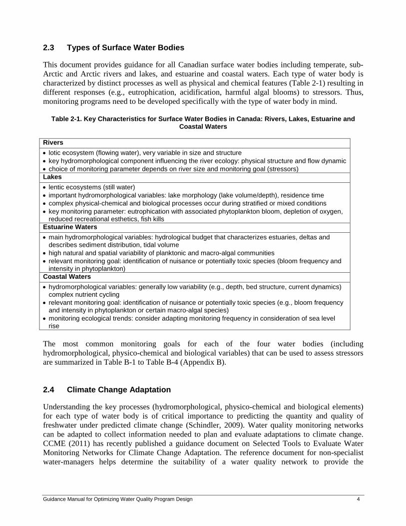
2.3 Types of Surface Water Bodies

This document provides guidance for all Canadian surface water bodies including temperate, sub-Arctic and Arctic rivers and lakes, and estuarine and coastal waters. Each type of water body is characterized by distinct processes as well as physical and chemical features (Table 2-1) resulting in different responses (e.g., eutrophication, acidification, harmful algal blooms) to stressors. Thus, monitoring programs need to be developed specifically with the type of water body in mind.

Table 2-1. Key Characteristics for Surface Water Bodies in Canada: Rivers, Lakes, Estuarine and Coastal Waters

Rivers • lotic ecosystem (flowing water), very variable in size and structure • key hydromorphological component influencing the river ecology: physical structure and flow dynamic • choice of monitoring parameter depends on river size and monitoring goal (stressors) Lakes • lentic ecosystems (still water) • important hydromorphological variables: lake morphology (lake volume/depth), residence time • complex physical-chemical and biological processes occur during stratified or mixed conditions • key monitoring parameter: eutrophication with associated phytoplankton bloom, depletion of oxygen,

reduced recreational esthetics, fish kills Estuarine Waters • main hydromorphological variables: hydrological budget that characterizes estuaries, deltas and

describes sediment distribution, tidal volume • high natural and spatial variability of planktonic and macro-algal communities • relevant monitoring goal: identification of nuisance or potentially toxic species (bloom frequency and

intensity in phytoplankton) Coastal Waters • hydromorphological variables: generally low variability (e.g., depth, bed structure, current dynamics)

complex nutrient cycling • relevant monitoring goal: identification of nuisance or potentially toxic species (e.g., bloom frequency

and intensity in phytoplankton or certain macro-algal species) • monitoring ecological trends: consider adapting monitoring frequency in consideration of sea level

rise The most common monitoring goals for each of the four water bodies (including hydromorphological, physico-chemical and biological variables) that can be used to assess stressors are summarized in Table B-1 to Table B-4 (Appendix B). 2.4 Climate Change Adaptation

Understanding the key processes (hydromorphological, physico-chemical and biological elements) for each type of water body is of critical importance to predicting the quantity and quality of freshwater under predicted climate change (Schindler, 2009). Water quality monitoring networks can be adapted to collect information needed to plan and evaluate adaptations to climate change. CCME (2011) has recently published a guidance document on Selected Tools to Evaluate Water Monitoring Networks for Climate Change Adaptation. The reference document for non-specialist water-managers helps determine the suitability of a water quality network to provide the


information needed to plan and adapt to a changing climate. Three approaches are presented to establish priorities to support climate change adaptation: • Basic Valuation Methods for Ecosystem Services • Ombrothermic Analysis • Water Resources Vulnerability Indicator Analysis.

In addition, three methods are discussed to evaluate the capacity and suitability of existing monitoring networks for climate change adaptation: • Audit Approach • Monte Carlo Network Degradation Approach • Multivariate Methods.

2.5 Selected Aspects of Water Quality Monitoring in Canada

CCME’s Canada-wide Framework for Water Quality Monitoring (CCME, 2006) was developed in 2006 with the aim to improve water resource management and to guide jurisdictions in the development and implementation of water quality monitoring programs in Canada. The framework provides high-level, consistent guidance for monitoring, program design, site selection, data management, interpretation and reporting. The framework identifies the need for greater coordination among jurisdictions in developing tools that could support a Canada-wide network of monitoring sites of interest. The Canadian Environmental Sustainability Indicators (CESI) freshwater water quality indicator (CCME, 2001a, 2001b) provides the Canadian public, policy analysts and decision makers with information about the status of water quality in Canada for the protection of aquatic life. Water Quality is assessed using CCME’s Water Quality Index (WQI). Newfoundland and Labrador actively participates in the CESI program every year and reports the findings. There is a portion of the Newfoundland and Labrador Department of Environment and Conservation web page that details the CESI program and displays most recent rankings for all core and local stations sampled in the province under the Canada-Newfoundland and Labrador Water Quality Monitoring Agreement. The Ministry of Sustainable Development, Environment and the Fight Against Climate Change of Québec operates a network of 260 water quality monitoring stations on the main rivers and other tributaries in Québec. The Department publishes data from these networks regularly to report on the state of water quality. The water quality is assessed using the Index of Bacteriological and Physicochemical Quality (IQBP). Finally, Environment Canada (EC) has produced a manual (EC, 2012a) outlining the steps that should be taken to assess the relative environmental risks to water quality monitoring sites included in EC’s long-term monitoring network using a risk-based approach (RBA).


2.6 Challenges of Water Quality Monitoring Networks

Common challenges for water quality monitoring networks are summarized by Lovett et al. (2007) and are listed below: • clear objectives and information expectations • appropriate spatial and temporal boundaries • quantitative evaluation of benefits of monitoring • integration of monitoring elements into data management systems • data-rich monitoring programs.

In addition to the scientific challenges identified above, there are financial constraints, changing government priorities, comparability of data across monitoring programs and the ability to sustain long term monitoring programs where results may not be evident for many years.

2.7 Water Quality Monitoring Network Optimization

Lovett et al. (2007) emphasize that water quality monitoring programs are the basis for the development of science-based environmental policies and discuss seven key aspects of highly successful monitoring programs: • designed around clear and compelling scientific questions • include review, feedback and adaptation in the design • carefully slected measurements with the future in mind • ensure consistent high data quality • consider long-term data accessibility and sample archiving • continuously examine, interpret and present monitoring data • integrated research program includes monitoring data.

Lovett et al. (2007) stress the importance of long-term studies because they provide: • data relating to ecosystem change (e.g., analysis of climate change impacts) • data required to discover emerging environmental issues • data to assess whether an event is unusual or extreme • critical information for designing appropriate research experiments • data for the evaluation of whether policies have had an intended effect.

Water quality management benefits from optimized cost-efficient water quality networks because they support sound decision-making and provide insight into how various ecosystem components interact. Well-designed monitoring systems result in lower costs for implementation and increased monetary benefits associated with environmental improvement (Lovett et al., 2007).


3.0 QUALITATIVE AND QUANTITATIVE TOOLS FOR EVALUATING WATER QUALITY MONITORING NETWORKS 3.1 Overview

Water quality is a complex topic and water quality monitoring networks have been developed to address different issues in water resource management. This section provides an overview of systematic and statistical science-based tools commonly used to assess the performance and efficiency of networks for optimization. Table 3-1. Summary of Quantitative and Qualitative Approaches for Different Design Aspects Used in

Optimizing Water Quality Monitoring and Corresponding Case Studies (Appendix A)

Design Aspect Evaluation Tool Case Study Reference

Definition of monitoring objectives

Data quality objective (DQO) Case Study 1 Case Study 2

Confidence interval, trend analysis

Case Study 3

Selection of water quality variables

Data quality objective (DQO) Case Study 1 Case Study 2


Case Study 3

Multivariate analysis Case Study 8

Spatial coverage Data quality objective (DQO) Case Study 1 Case Study 2


Case Study 3

Hierarchical structure, stream order approach

Case Study 4

Geospatial tools Case Study 5 Case Study 6 Case Study 7

Dynamic programming approach Case Study 9

Temporal frequency Data quality objective (DQO) Case Study 1 Case Study 2


Case Study 3

Entropy analysis Case Study 9

Spatio-Temporal frequency Artificial Neural Network

Case Study 11 Case Study 12

Dynamic Programming Case Study 10

Entropy Analysis Case Study 9

Table 3-1 summarizes the approaches presented in this section and gives reference to the case studies presented in Appendix A. The case studies are ordered based on level of complexity in the analysis involved for optimization. Table 3-1 also specifies the monitoring design aspects


(definition of objectives, selection of water quality variables, sample stations and temporal frequency) optimized in each case study. 3.2 Overview of Systematic Approaches

3.2.1 Data Quality Objective (DQO) Approach

The DQO process consists of seven steps as outlined in Table 3-2 (centre column). Step 1 identifies and clarifies the monitoring goals and objectives. Step 2 identifies required decisions. Steps 3 to 6 consider the technical aspects of network design including: variable selection, temporal frequency, site selection and period/duration of sampling. Step 7 involves data analysis and optimization of the design. These elements cannot be dissociated from each other and will be discussed further in this manual. Elements of the DQO process can be used to optimize water quality monitoring networks because it ensures that only data needed to support management decisions are collected. The process clarifies monitoring objectives, evaluates the appropriateness of the data (quality and quantity), and specifies tolerable levels of potential decision errors that will be required to support defensible management decisions. USEPA (2006a) provide detailed technical guidance on how to develop DQOs. The DQO process has been widely applied in the design and evaluation of water quality monitoring networks (Hunt et al., 2006, ASTWMO 2009). Clark et al. (2010) provide detailed descriptions on how to use the DQO processes with examples for aquatic ecosystems.

Table 3-2. Comparison of Steps in Water Quality Monitoring Activities and Steps in Data Quality Objective Process (DQO Process, US EPA, 2006a)

Step in Water Quality Monitoring Cycle (Figure 2-1)

Data Quality Objective Process (US EPA, 2006a) Step in DQO Content of Step

Step 1. Set Monitoring Objectives

Step 1: State the problem Conceptual model Step 2: Identify required decisions

Quantifiable monitoring objectives

Step 2. Monitoring Program Design

Step 3: Identify information inputs Variables (metrics, targets) Step 4: Define boundaries Spatial and temporal considerations

Step 3. Field Sampling Program/Laboratory Analyses and Procedures

Step 5. Develop the analytical approach Statistical analysis procedures

(mean, median, trend) Step 6. Specify tolerable limits/ limits on decision errors/ performance criteria

Level of uncertainty regarding monitoring decision outcomes

Step 4. Data Analysis and Interpretation

Step 7. Develop the detailed plan for obtaining data

Select the resource-effective sampling and analysis plan that meets the performance criteria

MacDonald et al. (2009) and Clark et al. (2010) describe a systematic, sequential, ecosystem-based framework for the design and evaluation of water quality monitoring programs that supports the management of aquatic ecosystems. The framework described by these authors is based on


experiences in Canadian watersheds, including a selection of temperate, sub-Arctic and Arctic rivers and lakes, ranging in elevation from sub-alpine to estuarine, ranging in turbidity from clear to highly turbid, and ranging in trophic status from oligotrophic to eutrophic. The approach proposed by MacDonald et al. (2009) and Clark et al. (2010) is consistent with the Data Quality Objective (DQO) process described by the USEPA (2006a). The DQO process was used to optimize the South Florida Water Management District’s (Hunt et al., 2006, Case Study 1, Appendix A) network which consists of more than 1500 monitoring sites.

3.2.2 Risk Based Approach

Environment Canada (EC, 2012a) has developed a risk based analysis (RBA) tool to assess the relative environmental risk to water quality and aquatic life at all EC water quality monitoring sites. Each site is assessed for three main categories of environmental risk: • sources of contaminants/activities that may affect water quality (stressors, point and non point

sources) • observed/potential water quality or aquatic ecosystem impacts (based on monitoring

information compared to guidelines, and effects on aquatic life) • vulnerability of the aquatic ecosystem (species at risk, importance of fishery, impaired water

uses).

The RBA tool assigns a risk score to each of several criteria associated with the three environmental risk categories. The total risk is calculated by summing the assessment scores for each of the criteria. The criteria also have weighting factors assigned to emphasize more important variables. The scores for these three main categories are then tabulated, and that score is normalized to a maximum total score of 100. Each site is then characterized as having low (0 – 30), moderate (30 – 70) or high risk (70 - 100), or having insufficient information on which to perform an assessment. A key advantage of this technique is that, similar to CCME’s Water Quality Index (CCME, 2001a), it provides a means to easily communicate the relative environmental risk at a given monitoring site on a scale from 0-100. By applying this technique to a number of water quality monitoring sites within watersheds it is possible to rank the location of monitoring sites in terms of environmental risk. This, in combination with other statistical techniques discussed in this manual, can provide a useful basis for making an informed decision when optimizing water quality networks. A caveat when using this technique is that it requires an in depth knowledge of the environmental factors in the immediate proximity of a monitoring site. Additionally, when multiple water quality practitioners are using the RBA tool care must be taken to ensure consistency in the application of the tool. A RBA guidance manual (EC, 2012a) has been developed to promote this consistency. Environment Canada is currently expanding the RBA to look at all sub drainage areas across Canada using a geospatial approach with readily available spatial datasets. The first phase involves looking at the first component of the RBA (i.e., sources of contaminants/activities that may affect water quality) and calculating the intensities of select stressor variables within the sub drainage area unit. Examples of some of the stressors include wastewater systems, pollutant releases to surface water, roads, dams, stream crossings, cropland, livestock manure, etc. Future phases will gather information on the other components of the RBA such as the vulnerability of the aquatic ecosystems


(e.g., sensitive waterbodies, protected areas, fisheries, etc.). The results will be used to assess the current EC monitoring network, help provide quantitative information for assessing monitoring sites using the RBA and to help identify gaps. The Risk Based Basin Analysis (RBBA) also creates a spatial geodatabase that can be used for future network design and for reporting and assessment of monitoring data. Similar type regional risk models have been developed by Saskatchewan, Alberta, and Nova Scotia.

3.2.3 Stream Order Hierarchical Approach

The stream ordering or hierarchical approach is a systematic approach to identify monitoring sites. The hierarchical approach was first proposed by Sharp (1971) and is based on the stream ordering concept (Horton, 1945). The steps involved for the hierarchical approach procedure are described in Table 3-3 and illustrated in Figure 3-1a-c. This method assigns each tributary of a river system an order of one (e.g., a first order tributary). A stream which is formed by the intersection of two first order tributaries is assigned an order of two (e.g., a second order tributary). This process of order assignment is continued until the mouth of the system is reached. The overall number of exterior tributaries considered is a question of judgment and depends on the scale of the map used. When order assignments are completed, the order of the final river section will be equal to the number of contributing tributaries.

Table 3-3. Hierarchical Approach: Steps Involved in Identifying First-, Second- and Third-Hierarchy Stations.

Steps Approach Step 1. Define the first-hierarchy reach Estimate the Centroid (C1) of a river stretch by dividing

the magnitude of the final stretch of the river by two (see Equation 3-1)

𝑪𝑪𝒊𝒊 = �𝑵𝑵𝟎𝟎+𝟏𝟏𝟐𝟐 � (Equation 3-1)

Ci: centroid, N0: stream order number at mouth of river If there is no link with this number, select the nearest in magnitude (e.g., example in Figure 3-1b, the first hierarchy station C1 would be placed at 9)

Step 2. Define the second-hierarchy reach Calculate centroids for the resulting two systems using Equation 3-1 (e.g., example in Figure 3-1b, the first hierarchy station C11(upstream) = 5 , C12(downstream) = 6)

Step 3. Define the third-hierarchy reach Calculate centroids for the resulting four subbasins using Equation 3-1. (e.g., example in Figure 3-1b, the first hierarchy station C111 = 2 , C112 = 2, C121 = 3 C122 = 3)

The first step in the hierarchical approach divides a river basin into first-hierarchy reaches by identifying the centroid of a basin where a first-hierarchy station would be placed. The second-hierarchy and third-hierarchy stations are then identified through successive subdivisions of the river network. Sampling stations are located at the downstream end of a river segment before an intersection (Sanders et al., 1983). Sanders et al. (1983) considered two levels of design criteria for location of sampling sites: the macro-location and the micro-location. The macro-locations are the river reaches that will be


sampled within the river basin, and they are defined using the stream ordering approach. Micro-locations refer to sampling locations within the reach that represent critical points such as outfalls or point sources of pollution. In network design, macro-locations are generally allocated systematically, while micro-locations are a function of macro-locations at critical points.

_

Figure 3-1. Location of Sampling Sites Using the Hierarchical Approach. a) Stream Orders in a River Network; b) First-, Second- and Third-Hierarchy Sites Using the Hierarchical

Approach Based on Stream Order, c) Hierarchical Approach Based on Biological Oxygen Demand Loading. Figures Adapted from Sanders et al. (1983)

The hierarchical approach can be used in situations where the locations of the sampling stations in a network have to be reassessed and relocated or can be used when initiating a monitoring network. It can also be used to define optimal spatial sampling intervals, and to identify critical areas and essential stream flow stations (Table 3-4).

Table 3-4. Advantages and Disadvantages of the Hierarchical Approach for Optimizing Spatial Coverage

5 2 2

1

9

2

233

2

62

5

19

4

4

Dam

5 2 2

1

6

9

32

23

15

32

6

2

5

19

4

4

74500

3945

5830

14129

1730

15580

2080

Hierarchy123

Hierarchy123

Hierarchy123

C11 C111C112

C122

C11

C1

C111

C112

C121

a) b) c)

C121

C12

C1

4220C12

C122

Tool Hierarchical Approach Description Divides basin in equal parts with respect to tributaries

Analysis of Design Aspect Spatial coverage

Advantages • Relocates sampling sites • Can be used for short-term datasets • Can be used in combination with attributes such as flow,

minimum area, pollution load Disadvantages • Crucial factor is the selection of tributaries or attributes to

be considered; this selection is subjective but can be minimized by judging on the basis of minimum flow, discharge volume, drainage area, contamination load (e.g., Figure 3-1c)


However, a disadvantage of this method is that the role of a specific tributary order may be under or over-emphasized: This approach is more applicable to smaller systems where there is a good understanding of the stressors. As systems become larger and more complex, there is more potential for redundancy and less potential to capture cumulative stressors. Generally, each tributary in a river system does not make an equivalent contribution to the larger river system. To compensate for this, the hierarchical approach can be modified and other characteristics such as stream attributes (e.g., discharge volume or drainage area) or contamination loads (BOD5) can be considered to give a true weight to each tributary. The use of the hierarchical approach for optimizing the spatial coverage in water quality monitoring networks is described in Case Study 4 Gediz River, Turkey (Harmancioǧlu et al., 1999) in Appendix A. 3.3 Overview of Statistical Approaches

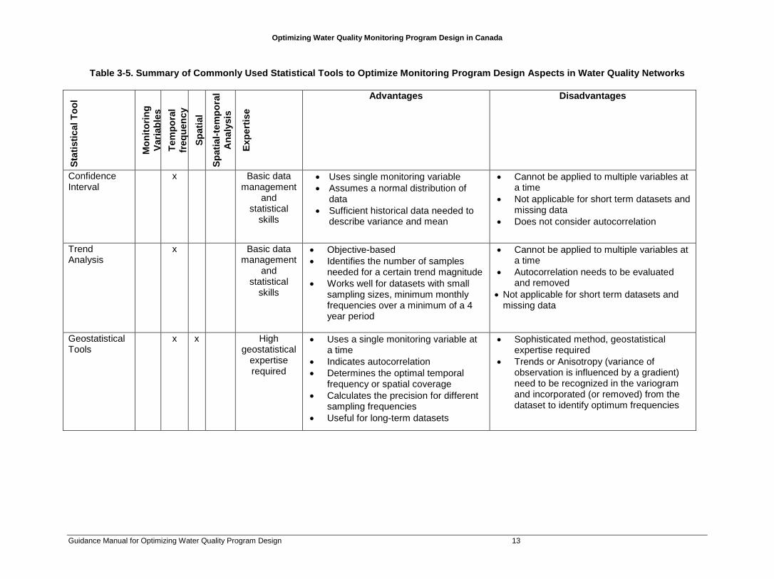
There are a number of statistical tools that can be applied to optimize the technical aspects of water quality monitoring program design: determination of water quality variables, sampling frequency and spatial distribution of sampling locations. Khalil and Ouarda (2009) provide an up-to-date detailed review of statistical approaches commonly used for the technical design of surface water quality monitoring networks. A brief summary of these approaches is provided in Table 3-5. References for case studies and more detailed descriptions of the techniques are included in the following text for each approach. It should be noted that each of the statistical approaches assume that previously collected data can inform the development of optimal monitoring design for the future. However, a potential drawback is that aquatic ecosystems are dynamic and the approaches that worked in the past may not always be ideal going forward. Therefore, the periodic evaluation of a water quality monitoring network (see Step 3) is imperative to ensure the effectiveness of the network and that monitoring objectives are still met.


Optimizing Water Quality Monitoring Program Design in Canada

Table 3-5. Summary of Commonly Used Statistical Tools to Optimize Monitoring Program Design Aspects in Water Quality Networks St

atis

tical

Too

l

Mon

itorin

g Va

riabl

es

Tem

pora

l fr

eque

ncy

Spat

ial

Sp

atia

l-tem

pora

l A

naly

sis

Expe

rtis

e

Advantages Disadvantages

Confidence Interval

x Basic data management

and statistical

skills

• Uses single monitoring variable • Assumes a normal distribution of

data • Sufficient historical data needed to

describe variance and mean

• Cannot be applied to multiple variables at a time

• Not applicable for short term datasets and missing data

• Does not consider autocorrelation

Trend Analysis


and statistical

skills

• Objective-based • Identifies the number of samples

needed for a certain trend magnitude • Works well for datasets with small

sampling sizes, minimum monthly frequencies over a minimum of a 4 year period

• Cannot be applied to multiple variables at a time

• Autocorrelation needs to be evaluated and removed


Geostatistical Tools

x x High geostatistical

expertise required

• Uses a single monitoring variable at a time

• Indicates autocorrelation • Determines the optimal temporal

frequency or spatial coverage • Calculates the precision for different

sampling frequencies • Useful for long-term datasets

• Sophisticated method, geostatistical expertise required

• Trends or Anisotropy (variance of observation is influenced by a gradient) need to be recognized in the variogram and incorporated (or removed) from the dataset to identify optimum frequencies



Stat

istic

al T

ool

Mon

itorin

g Va

riabl

es

Tem

pora

l fr

eque

ncy

Spat

ial

Sp

atia

l-tem

pora

l A

naly

sis

Expe

rtis

e


Correlation and Regression Analysis

x Basic to moderate

data management

and statistical

skills

• Optimizes multiple variables for a single site at a time

• Can be used for smaller datasets • Allows the reconstitution of

information about the discontinued variables using regression analysis

• Associating of two variables can be problematic, criteria to decide when two variables are correlated is subjective (different outcomes possible)

• Reproducibility can be low, due to subjectivity in deciding the selection of the proper threshold above which a correlation coefficient can be considered sufficient

Hierarchical Approach


and statistical

skills

• Relocates sampling sites • Can be used for short-term

datasets • Can be used in combination with

attributes such as flow, minimum area, pollution load

• Crucial factor is the selection of tributaries or attributes to be considered, This selection is subjective but can be minimized by judging on the basis of minimum flow, discharge volume, or contamination load

Multivariate Analysis

x x x Moderate: Multivariate statistical expertise required, database

management

• Optimizes multiple variables at a time

• Performs very well for datasets with linear distribution

• Can be used for smaller datasets (minimum 1 year, minimum ~ 50 datapoints)

• Statistical and multivariate statistical expertise required

• Data needs to be transformed and standardized


Principal Component Analysis (PCA)

x x • Extracts ecological gradients of maximum variation

• Assumes linear relationship to ecological gradients



Stat

istic

al T

ool

Mon

itorin

g Va

riabl

es

Tem

pora

l fr

eque

ncy

Spat

ial

Sp

atia

l-tem

pora

l A

naly

sis

Expe

rtis

e


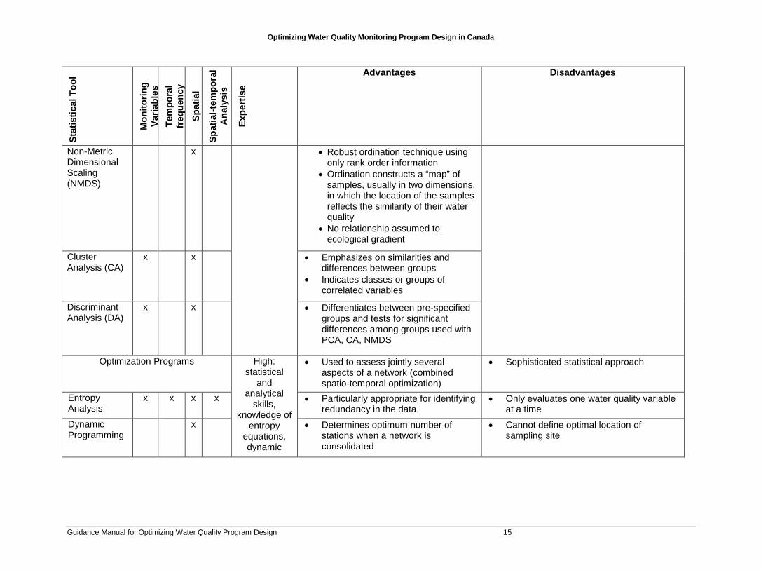
Non-Metric Dimensional Scaling (NMDS)

x • Robust ordination technique using only rank order information

• Ordination constructs a “map” of samples, usually in two dimensions, in which the location of the samples reflects the similarity of their water quality

• No relationship assumed to ecological gradient

Cluster Analysis (CA)

x x • Emphasizes on similarities and differences between groups

• Indicates classes or groups of correlated variables

Discriminant Analysis (DA)

x x • Differentiates between pre-specified groups and tests for significant differences among groups used with PCA, CA, NMDS

Optimization Programs High: statistical

and analytical

skills, knowledge of

entropy equations, dynamic

• Used to assess jointly several aspects of a network (combined spatio-temporal optimization)

• Sophisticated statistical approach

Entropy Analysis

x x x x • Particularly appropriate for identifying redundancy in the data

• Only evaluates one water quality variable at a time

Dynamic Programming

x • Determines optimum number of stations when a network is consolidated

• Cannot define optimal location of sampling site



Stat

istic

al T

ool

Mon

itorin

g Va

riabl

es

Tem

pora

l fr

eque

ncy

Spat

ial

Sp

atia

l-tem

pora

l A

naly

sis

Expe

rtis

e


Artificial Neural Network (ANN)

x programming and ANN

• Promising modeling tool in integrated water management

• No assumptions need to be made and the pre-processing of data is minimal.

• Only works within the boundaries of a certain situation


3.3.1 Introduction to Statistical Testing: Decision-Errors

An important aspect in the analysis of water quality monitoring data is the understanding of the types of decision errors associated with the statistical analysis and hypothesis test (null hypothesis H0 or alternative hypothesis Ha). Four outcomes often have to be considered: two outcomes lead to the correct decision being made regarding the monitoring data and the other two outcomes represent decision errors (Table 3-6). A false rejection error (also called a Type I error) occurs when the null hypothesis is true, but is rejected: the probability that this error will occur is called alpha (α). A false acceptance error (also called a Type II error) occurs when the null hypothesis is false, but is accepted: the probability that this error will occur is called beta (β) (USEPA, 2006a). The Type II error can be set at 10% when determining the amount of change or differences that can be practically detected by existing monitoring programs (European Communities, 2003). An important consideration for water quality monitoring is that a Type I error (e.g., water body with good water quality is misclassified) may lead to unnecessary measures that can lead to substantial additional cost. However, implications for a Type II error (e.g., water body with marginal water quality was not identified) could be even more dramatic, because the potential risks of significant damage were not identified.

Table 3-6. Decision Errors and Possible Outcomes from Statistical Hypothesis Testing (from USEPA, 2006a)

Decision made by applying the statistical hypothesis test to the monitoring data

Decide that the null hypothesis H0 is true

Decide that the alternative hypothesis H1 is true

True Condition (reality)

H0 is true Correct decision Error Type I, False positive, probability α H0 is rejected when it is actually true

Implication None Unnecessary measures can lead to substantial costs

HA is true Error Type II (False negative), probability β H1 is rejected, when it is actually true

Correct decision

Implication Fail to identify risks of significant damage that could be averted

None

3.3.2 Confidence Intervals to Estimate Sampling Frequency

The mean is the most commonly reported statistical parameter for water quality data. Sanders et al. (1983) recommend using the confidence intervals about the mean as the main criterion for


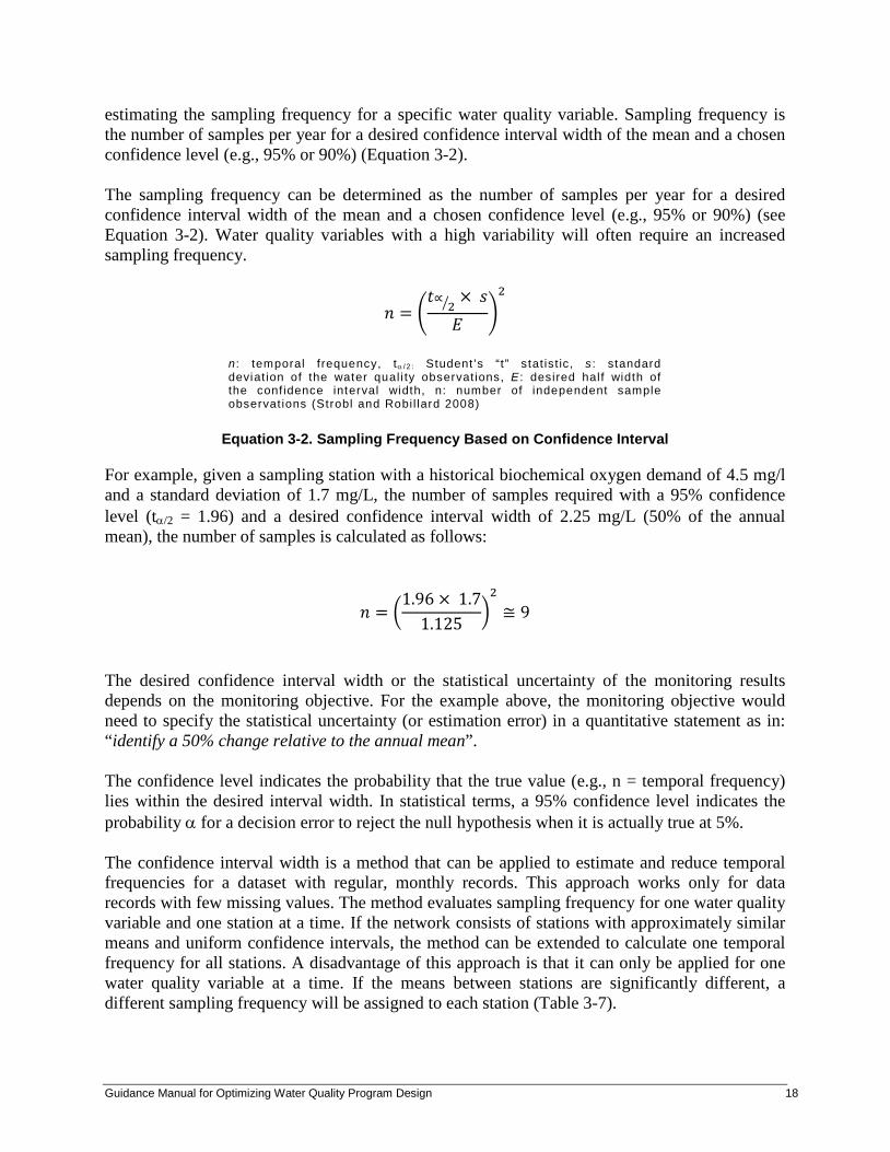
estimating the sampling frequency for a specific water quality variable. Sampling frequency is the number of samples per year for a desired confidence interval width of the mean and a chosen confidence level (e.g., 95% or 90%) (Equation 3-2). The sampling frequency can be determined as the number of samples per year for a desired confidence interval width of the mean and a chosen confidence level (e.g., 95% or 90%) (see Equation 3-2). Water quality variables with a high variability will often require an increased sampling frequency.

𝑛𝑛 = �𝑡𝑡∝

2�× 𝑠𝑠𝐸𝐸

�2

n : temporal f requency, tα / 2 : Student ’s “t” stat ist ic, s : standard deviat ion of the water qual i ty observat ions, E : desired half width of the conf idence interval width, n: number of independent sample observat ions (Strobl and Robil lard 2008)

Equation 3-2. Sampling Frequency Based on Confidence Interval

For example, given a sampling station with a historical biochemical oxygen demand of 4.5 mg/l and a standard deviation of 1.7 mg/L, the number of samples required with a 95% confidence level (tα/2 = 1.96) and a desired confidence interval width of 2.25 mg/L (50% of the annual mean), the number of samples is calculated as follows:

𝑛𝑛 = �1.96 × 1.7

1.125�2

≅ 9 The desired confidence interval width or the statistical uncertainty of the monitoring results depends on the monitoring objective. For the example above, the monitoring objective would need to specify the statistical uncertainty (or estimation error) in a quantitative statement as in: “identify a 50% change relative to the annual mean”. The confidence level indicates the probability that the true value (e.g., n = temporal frequency) lies within the desired interval width. In statistical terms, a 95% confidence level indicates the probability α for a decision error to reject the null hypothesis when it is actually true at 5%. The confidence interval width is a method that can be applied to estimate and reduce temporal frequencies for a dataset with regular, monthly records. This approach works only for data records with few missing values. The method evaluates sampling frequency for one water quality variable and one station at a time. If the network consists of stations with approximately similar means and uniform confidence intervals, the method can be extended to calculate one temporal frequency for all stations. A disadvantage of this approach is that it can only be applied for one water quality variable at a time. If the means between stations are significantly different, a different sampling frequency will be assigned to each station (Table 3-7).


Table 3-7. Advantages and Disadvantages of Confidence Interval for Optimizing Spatial coverage

Tool Confidence Interval

Description Uses the mean of a monitoring variable to determine sample numbers

Analysis of Design Aspect

Temporal frequency

Advantages • Uses single monitoring variable • Sufficient historical data (regular monthly records) needed

to describe variance and mean Disadvantages • Cannot be applied to multiple variables at a time

• Assumes a normal distribution of data • Not applicable for short term datasets and missing data

Swertz et al. (1997) in Case Study 3 (Appendix A) used confidence intervals to optimize temporal frequency for monitoring Dutch coastal waters. Temporal frequency was optimized for several variables and different media (e.g., water, suspended matter, sediment and organisms). The authors provided recommendations for more cost-efficient and effective monitoring.

3.3.3 Trend Analysis to Determine Sample Frequency

Trend analysis, in addition to identifying a data trend, can also be used to determine the optimum temporal frequency in a long-term monitoring network design where monitoring objectives relate to the detection of trends. The statistical statement for such a monitoring objective needs to specify the magnitude of the trend to be estimated (e.g., before and after mean of a contaminant concentration or load, or slope of a trend line for temperature change or water quality index), the desired confidence level associated with any assertion that a change has been detected and the Type II error (see Section 3.3.1, page 17). A long-term trend monitoring program involves the collection of samples at regular time intervals (e.g., monthly, yearly) over an extended period. Statistical tests commonly used for trend detection (e.g., Mann-Kendall, Sen`s slope estimator) are summarized in USEPA (2006b). The trend analysis approach (Lettenmeier, 1976) consists of two steps: the first step identifies the maximum number of samples that can be collected per year. The second step estimates the length of a record needed to detect trends at specified confidence intervals and test powers. Each of these steps is described below. The sampling frequency required to achieve independent samples includes the evaluation of autocorrelation (serial and seasonal correlation) between measurements (Step 1). Serial and seasonal correlation is frequently present in long-term data sets and needs to be quantified and removed prior to trend analysis. Serial correlation occurs if a water quality variable of interest is collected close enough together in time so that each observation is most similar and related to the adjacent observation. Seasonal correlations occur when the water quality variable of interest varies seasonally. Methods for estimating serial and seasonal autocorrelation and how to remove


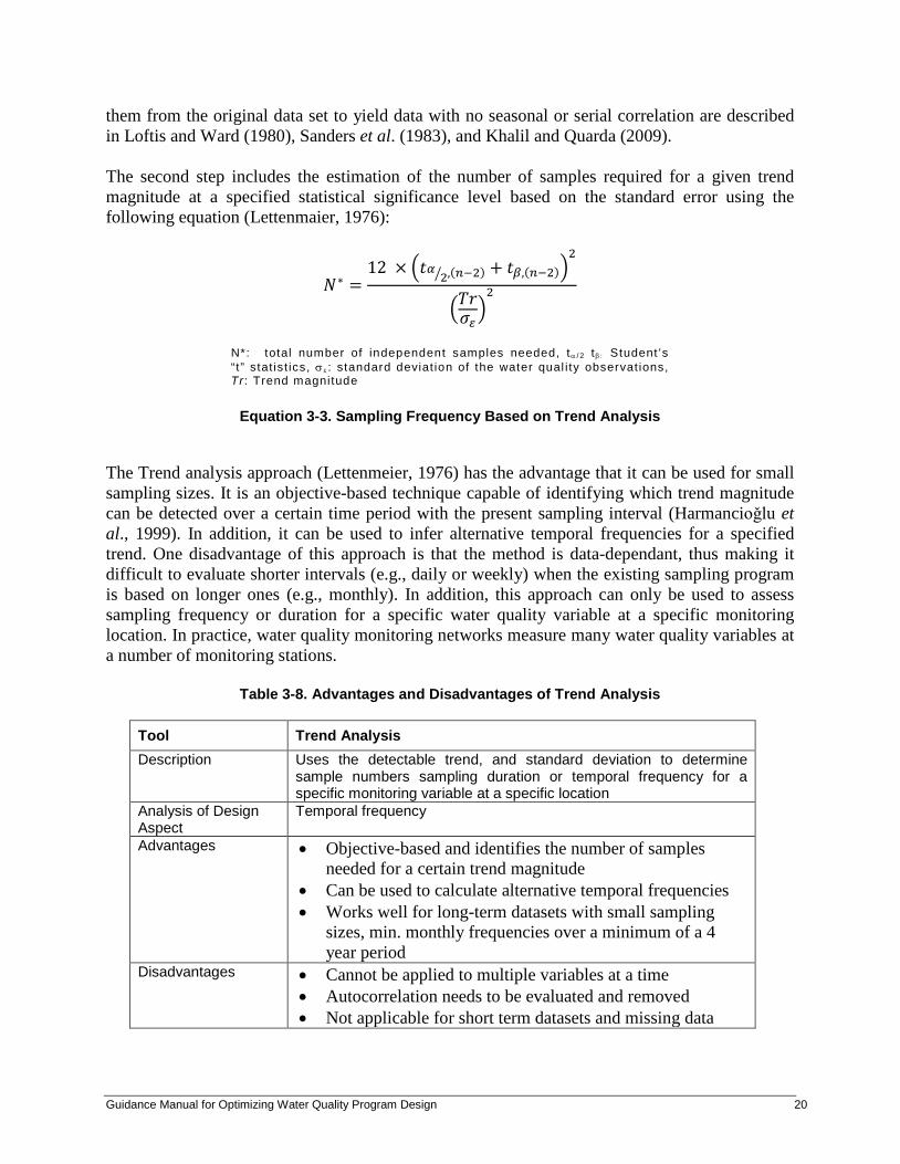
them from the original data set to yield data with no seasonal or serial correlation are described in Loftis and Ward (1980), Sanders et al. (1983), and Khalil and Quarda (2009). The second step includes the estimation of the number of samples required for a given trend magnitude at a specified statistical significance level based on the standard error using the following equation (Lettenmaier, 1976):

𝑁𝑁∗ =12 × �𝑡𝑡𝛼𝛼

2� ,(𝑛𝑛−2) + 𝑡𝑡𝛽𝛽,(𝑛𝑛−2)�2

�𝑇𝑇𝑇𝑇𝜎𝜎𝜀𝜀�2

N*: total number of independent samples needed, tα / 2 tβ : Student ’s “t” stat ist ics, σε: standard deviat ion of the water qual i ty observat ions, Tr : Trend magnitude

Equation 3-3. Sampling Frequency Based on Trend Analysis

The Trend analysis approach (Lettenmeier, 1976) has the advantage that it can be used for small sampling sizes. It is an objective-based technique capable of identifying which trend magnitude can be detected over a certain time period with the present sampling interval (Harmancioǧlu et al., 1999). In addition, it can be used to infer alternative temporal frequencies for a specified trend. One disadvantage of this approach is that the method is data-dependant, thus making it difficult to evaluate shorter intervals (e.g., daily or weekly) when the existing sampling program is based on longer ones (e.g., monthly). In addition, this approach can only be used to assess sampling frequency or duration for a specific water quality variable at a specific monitoring location. In practice, water quality monitoring networks measure many water quality variables at a number of monitoring stations.

Table 3-8. Advantages and Disadvantages of Trend Analysis

Tool Trend Analysis Description Uses the detectable trend, and standard deviation to determine

sample numbers sampling duration or temporal frequency for a specific monitoring variable at a specific location


Temporal frequency

Advantages • Objective-based and identifies the number of samples needed for a certain trend magnitude

• Can be used to calculate alternative temporal frequencies • Works well for long-term datasets with small sampling

sizes, min. monthly frequencies over a minimum of a 4 year period

Disadvantages • Cannot be applied to multiple variables at a time • Autocorrelation needs to be evaluated and removed • Not applicable for short term datasets and missing data


Hunt et al., 2006 (Case Study 1, Appendix A) used the Seasonal Kendall Tau Test for trend analysis to optimize the water quality monitoring network of the South Florida Water Management District. Monte Carlo simulations using the Seasonal Kendall Tau Test for Trend were performed to estimate the power to detect a trend for a given water quality parameter. A 20% change (power of 0.8) in slope of any given water quality parameter over a five year time period was used as a target change for detection. The power analysis procedure estimated the annual percent change that the monitoring program was able to detect. Swertz et al. 1997 (Case Study 3) analyzed monitoring results for several different media (water, suspended matter, sediment and organisms) over a five year period to establish the minimum detectable trend. By also considering the cost of analyzing different media, the authors concluded that monitoring to detect trends in this network was most effective in suspended matter and sediment. Swertz et al. (1997) also used trend analysis for frequency optimization and concluded that the optimum number of observations for this network was between 10 and 20 samples per year.

3.3.4 Additional Considerations to Temporal Frequency

The temporal frequency in a monitoring program network depends on the monitoring objectives. These should clearly identify data requirements such as the precision or statistical uncertainty (estimated error) of the monitoring results as a quantitative statement (e.g., degree of difference relative to the water quality criteria, a percentile, the slope of a linear trend, or confidence levels). Relationships between confidence level, sampling frequency, statistical uncertainty and variability are illustrated and described in more detail below. The relationships between confidence levels, precision and number of samples are demonstrated in the following examples. In this example, sample frequency (expressed as number of samples) is shown in relation to the precision (expressed as the % change relative to the mean) for three confidence limits (80%, 90% and 95%). Precision improves (error is reduced) with increased sampling frequency For example, Figure 3-2 illustrates that 15 samples are required to achieve an precision of 30% at a 95% confidence level, 10 samples are required at a 90% confidence level and only 7 samples at an 80% confidence level. However, an important consideration is that a low level of confidence to achieve a high degree of precision results in only questionable savings: larger confidence intervals correspond to a higher degree of uncertainty. Generally, a 90 or 95% confidence level is recommended for water quality data.


_

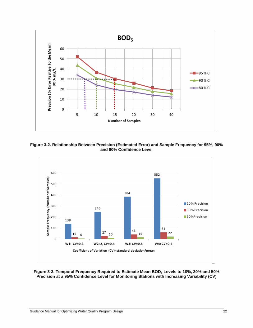
Figure 3-2. Relationship Between Precision (Estimated Error) and Sample Frequency for 95%, 90% and 80% Confidence Level

_

Figure 3-3. Temporal Frequency Required to Estimate Mean BOD5 Levels to 10%, 30% and 50% Precision at a 95% Confidence Level for Monitoring Stations with Increasing Variability (CV)

0

10

20

30

40

50

60

5 10 15 20 30 40

Prec

ision

( %

Err

or R

ealti

ve t

o th

e M

ean)

BO

D 5 m

g/L

Number of Samples

BOD5

95 % CI

90 % CI

80 % CI

138

246

384

552

15 27 43 61

6 10 15 22

0

100

200

300

400

500

600

W1: CV=0.3 W2: 2, CV=0.4 W3: CV=0.5 W4: CV=0.6

Sam

ple

Freq

uenc

y (N

umbe

r of S

ampl

es)

Coefficient of Variation (CV)=standard deviation/mean

10 % Precision

30 % Precision

50 %Precision


_

Figure 3-4. Relationship Between Coefficient of Variation and Error of Expected Results for 5, 10, 15 and 20 Samples Collected within the Year

Figure 3-3 shows the relationship between sample frequency and variability for three different errors (10%, 30% and 50%) using a 95% confidence level. Variability in Figure 3-3 is expressed as the coefficient of variation (CV), which is defined as the standard deviation divided by the mean. The four stations W1-W4 are arranged according to increasing variability. Higher sampling frequencies are required for water quality variables with a higher variability to achieve the same degree of uncertainty. A monitoring variable with a coefficient of variation of 0.3 and a sample frequency of 10 can yield a maximum precision of 35%, while a parameter with a higher coefficient of variation (e.g., 0.6) can yield a maximum precision of 80% at a sample frequency of 10. Figure 3-4 illustrates the relationship between temporal frequency and precision expressed as (% change relative to the mean) for different sample sizes (5, 10, 15 and 20).

3.3.5 Correlation Analysis and Regression Analysis

The correlation and regression analysis method for reducing the number of water quality variables is based on three steps, as described in Table 3-9:

0

20

40

60

80

100

120

0.3 0.4 0.5 0.6

Prec

ision

(%

Err

or R

ealti

ve t

o th

e M

ean)

Coefficient of Variation (standard deviation/mean)

n = 5 samples

n=10 samples

n = 15 samples

n= 20 samples


Table 3-9. Summary of Steps for the Correlation and Regression Analysis for Optimizing Water Quality Variables

Steps Description Step 1. Correlation analysis is performed and is used to measure the strength of the association

between two monitoring parameters; a high correlation coefficient indicates that some of the information produced is redundant and perhaps one of the monitoring variables can be discontinued.

Step 2. Selection of monitoring variables that can be discontinued has to be evaluated against the monitoring objectives and based on professional judgment (e.g., qualitative criteria such as cost of analysis, significance of parameter).

Step 3. Regression analysis is used to reconstruct the information about the discontinued variables using auxiliary variables from those variables that are continuously measured. Thus, the original list of variables being measured becomes partially measured, and partially estimated using regression analysis.

Correlation analysis does not imply cause and effect. A high correlation between two variables indicates a strong relationship, but does not allow conclusions on which variable causes the other variable to increase or decrease without examination evidence and strong statistical controls. Professional judgment is required to develop criteria to identify which water quality variables should be retained or discarded. Furthermore, these considerations need to include the significance of the water quality variable with respect to the monitoring objective and can also include factors such as analytical cost or the variance of the mean. Care must be taken to ensure that core monitoring parameters remain in the program. For example, correlation analysis of a water quality variable dataset suggests that the levels of major ions such as chloride, sulphate, potassium, magnesium and carbonates are strongly correlated. The parameters to measure continuously have to be evaluated against the monitoring objective. If the monitoring objective is related to atmospheric deposition (e.g., acid rain) sulphate should be selected as the core parameter. However if the objective is related to de-icing activities, chloride should be retained as the core parameter. In this case, conductivity or salinity could also be selected as an indicator parameter for the ionic constituents. Regression analysis can be performed to reconstruct the information for the various ions. Similarly, concentrations of the major forms of nutrients (e.g., ammonia, nitrite and nitrate; or total phosphorus and dissolved phosphorus) could be correlated in a water quality dataset for a lake. If the monitoring objective is related to the identification of a trend in eutrophication, all major forms of a nutrient should be continuously measured as they provide key information on the nutrient cycles and trophic conditions within the system. The correlation and regression analysis approach works well for a water quality network consisting of suites of water quality variables that are associated with certain types of stressors (e.g., total PCBs rather than individual PCB congener analysis). An advantage of this approach is that the information regarding discontinued water quality variables can be reconstructed using regression techniques (Khalil and Quarda, 2009). However, a deficiency of this method is the absence of a criterion to identify those monitoring parameters that should be discontinued or continuously measured. Another deficiency is that this approach can be used for only one station at a time: results in a network where different water quality variables are measured at different stations cannot be evaluated. This is exacerbated by the fact that, in most water quality monitoring networks, several variables are measured simultaneously (Table 3-10).


Correlation and regression analysis can also be used to evaluate spatial coverage. In this case, the spatial correlation between the monitoring stations is evaluated for each water quality monitoring parameter one at a time.

Table 3-10. Advantages and Disadvantages of Using the Correlation and Regression Analysis

Tool Correlation and Regression Analysis

Description Calculates correlation between variables and regression equations for variables that will be discontinued


Monitoring variables, spatial coverage

Advantages • Optimizes multiple variables for a single site at a time • Can be used for smaller datasets • Allows the reconstitution of information about the discontinued

variables using regression analysis Disadvantages • Associating two variables can be problematic, professional judgment

needed to decide on criteria when two variables are correlated (e.g., analytical costs could be used)

• Reproducibility can be low, due to subjectivity in deciding the selection of the proper threshold above which a correlation coefficient can be considered sufficient.

Hunt et al. (2006) used correlation analysis to optimize the South Florida Water Management District’s network (Case Study 1, Appendix A) and to evaluate the correlations between sampling stations (for specific parameters) as well as to evaluate correlations between all parameters for a given project. In Case Study 2, Hunt et al. (2008) (Appendix A) used correlation analysis to characterize the relationship between annual average readings with a reduced monitoring strategy for dissolved oxygen and chlorophyll. Reductions in the number of sampling stations were found less detrimental to the quality of the data for annual decision-making than reductions in the number of surveys per year for this particular monitoring network. In Case Study 3, Swertz et al. (1997) conducted a correlation study to examine the extent to which observations at one monitoring site could be used to predict the results at another station (Appendix A). It was found that concentrations of dissolved substances at sites several kilometres apart could be used to predict each other with an accuracy of over 90%. In terms of correlation over time (the autocorrelation), the study found that monitoring at intervals of less than one month provided redundant data in marine water areas.

3.3.6 Geostatistical Tools

Geostatistical tools such as a semivariogram are common tools used to assess spatial or temporal correlations and can be used to evaluate temporal frequencies in a water quality monitoring


network. The semivariogram method is based on the fundamental work of Krige (1951) and Matheron (1963) and is a graphical representation of how the similarity between pairs of observations varies as a function of distance or time.

Table 3-11. Advantages and Disadvantages of Using Geostatistical Tools

Tool Geostatistical Tools

Description Estimates a variogram that defines the distance over which sampling sites or sampling frequency are representative


Temporal frequency, spatial coverage

Advantages • Uses a single monitoring variable at a time • Indicates autocorrelation • Determines the optimal temporal or spatial coverage • Calculates the precision for different sampling frequencies • Useful for long-term datasets

Disadvantages • Sophisticated method, geostatistical expertise required • Trends or Anisotropy (variance of observation is influenced by a

gradient) need to be recognized in the variogram and incorporated (or removed) from the dataset to identify optimum frequencies

Geostatistical software can be used to plot a semivariogram for the water quality data collected at monitoring station over time. The semivariogram is the first step in geostatistical analysis. It describes the correlation structure among observations (e.g., water quality measurements) and indicates the distance over which sampling sites or sampling intervals are representative and independent from each other. In a second step, the information provided by the variogram is used to estimate the precision (prediction error) at discrete distances (time, locations) using interpolation procedure such as kriging (Dowdall et al., 2005). Geostatistical tools are useful because they describe patterns among observations and help to identify autocorrelation. The information of a variogram can be used to assess the precision achieved at different sampling frequencies for a water quality monitoring network. A disadvantage of this method is that the assistance of a geostatistical expert may be required to evaluate long-term datasets and identify if the assumptions of the model are met (EC, 2012b) (Table 3-12). The case studies described in detail in Appendix A used geospatial tools to optimize water quality networks. Dowdall et al. (2005) (Case Study 7) utilized geostatistical techniques in the optimization and design of sampling regimes to monitor temporal fluctuations in the levels of technetium in the Norwegian Arctic marine environment. Beveridge et al. (2012) (Case Study 6) used geostatistical methods to quantify redundancy in a dense network of lake monitoring stations in Lake Winnipeg. Two approaches were used: 1) kriging and 2) local Moran’s I values were calculated to identify clusters of stations that were similar or different.


3.3.7 Multivariate data analysis

Multivariate data analysis techniques are useful tools that have been commonly employed in optimization of water quality monitoring networks. Multivariate techniques have the advantage that they assess multiple parameters simultaneously. Common multivariate procedures used in water quality optimization include ordination techniques such as principal component analysis (PCA) and non-metric dimensional scaling (NMDS), classification techniques such as cluster analysis (CA) as well as discrimination techniques such as discriminant analysis (DA). Ordination techniques such as PCA and NMDS can be applied to identify redundancy in the water quality variables measured within a monitoring network and to reduce the number of variables measured. Ordination constructs a “map” of samples, usually in two dimensions, in which the location of the samples reflect the (dis)similarity of two stations based on their water quality. Distances between samples match the corresponding (dis)similarities: nearby sites have very similar water quality, while samples that are far apart have different water quality. PCA transforms a set of correlated variables into a smaller set of uncorrelated variables. PCA performs optimally if the water quality data are linear and a normal distribution of the data is assumed. PCA can also be used to evaluate spatial redundancy. NMDS is the most robust ordination technique and uses only rank order information to construct a map where distances between sample sites have the same rank order as the corresponding dissimilarities between samples (Clarke and Warwick, 2001). CA is a classification technique commonly used to group similar observations into clusters, where the within-cluster variance is minimized and the between-cluster variance is maximized. For water quality monitoring networks, cluster analysis can be used to identify groups of similar sampling stations. DA is a discrimination technique used to differentiate between pre-specified groups resulting from PCA, NMDS or CA techniques. DA can also be used to test for significant differences among groups. Details concerning PCA, NMDS, CA and DA are available in reference text books (e.g., Tabachnick and Fidell, 1996, Clarke and Warwick, 2001). An advantage of using multivariate techniques is that they allow the examination of spatial and temporal trends because they assess many variables simultaneously. However, many multivariate analysis techniques suffer from the limitation of assuming a linear model. Multivariate methods such as PCA, NMDS, CA and DCA generally provide good results, thus a non-normal dataset does not necessarily eliminate the utility of this strategy (Table 3-12).A disadvantage in using PCA for identification of station redundancy is the absence of a criterion to identify the combination of variables to be continually measured or discontinued. Total cost of lab analysis for each combination of variables could be used as a criterion to rank possible combinations (Khalil and Quarda, 2009).


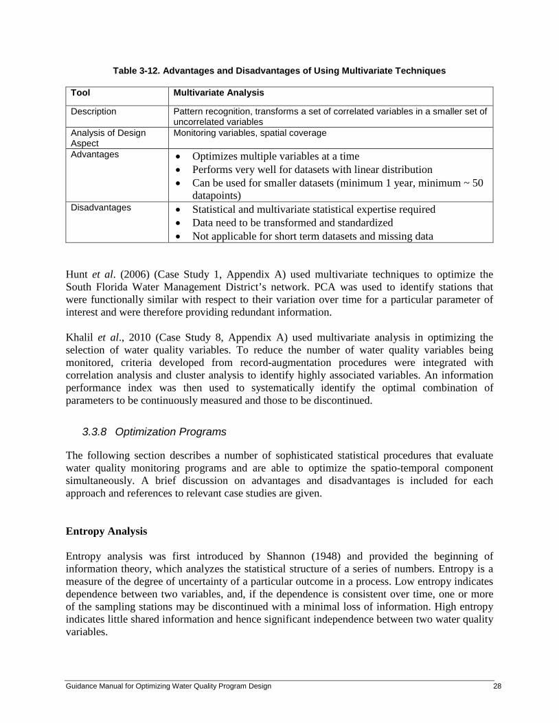
Table 3-12. Advantages and Disadvantages of Using Multivariate Techniques

Hunt et al. (2006) (Case Study 1, Appendix A) used multivariate techniques to optimize the South Florida Water Management District’s network. PCA was used to identify stations that were functionally similar with respect to their variation over time for a particular parameter of interest and were therefore providing redundant information. Khalil et al., 2010 (Case Study 8, Appendix A) used multivariate analysis in optimizing the selection of water quality variables. To reduce the number of water quality variables being monitored, criteria developed from record-augmentation procedures were integrated with correlation analysis and cluster analysis to identify highly associated variables. An information performance index was then used to systematically identify the optimal combination of parameters to be continuously measured and those to be discontinued.

3.3.8 Optimization Programs

The following section describes a number of sophisticated statistical procedures that evaluate water quality monitoring programs and are able to optimize the spatio-temporal component simultaneously. A brief discussion on advantages and disadvantages is included for each approach and references to relevant case studies are given.

Entropy Analysis Entropy analysis was first introduced by Shannon (1948) and provided the beginning of information theory, which analyzes the statistical structure of a series of numbers. Entropy is a measure of the degree of uncertainty of a particular outcome in a process. Low entropy indicates dependence between two variables, and, if the dependence is consistent over time, one or more of the sampling stations may be discontinued with a minimal loss of information. High entropy indicates little shared information and hence significant independence between two water quality variables.

Tool Multivariate Analysis

Description Pattern recognition, transforms a set of correlated variables in a smaller set of uncorrelated variables


Monitoring variables, spatial coverage

Advantages • Optimizes multiple variables at a time • Performs very well for datasets with linear distribution • Can be used for smaller datasets (minimum 1 year, minimum ~ 50

datapoints) Disadvantages • Statistical and multivariate statistical expertise required

• Data need to be transformed and standardized • Not applicable for short term datasets and missing data


Entropy analysis can be used to evaluate water quality and hydrometric networks (Ozkul et al., 2000). The fundamental concept in designing or optimizing water quality networks using entropy analysis is that sample locations must be independent from each other and share very little information. Entropy analysis reflects the spatial and/or temporal variability of water quality. The entropy approach is particularly appropriate for identifying redundancy in the data. Mishra et al. (2010) used entropy analysis approach to identify essential streamflow stations and critical areas such as poor network density in the Canadian setting. The most deficient hydrometric networks were identified in Alberta (North Saskatchewan, Oldman, and Red Deer basins), Northern Ontario (Hudson Bay basin), and the Northwest Territories. Entropy analysis is an efficient tool for evaluating network effectiveness and cost-efficiency, because this method can assess several aspects of network design, including: • spatial coverage • temporal frequencies • combined space/time frequencies • sampling duration • termination of collection program • cost-efficiency and • optimum number of samples.

Entropy analysis can also be applied in combination with other methods, such as multivariate techniques. The major disadvantage of using the entropy method is that it only evaluates one water quality variable at a time. The choice of time interval for which the water quality variables are assigned also has a significant impact on the accuracy of the results. In the case of analyzing station redundancy, the method cannot define where exactly new stations should be located and gives preference to stations with long records (Khalil and Ouarda, 2009). Ozkul et al., 2000 (Case Study 9, Appendix A) used entropy analysis to evaluate spatial coverage, temporal sampling frequencies, and combined space/time network features. The procedure developed for spatial design produced a priority list of stations to be retained in the network such that each new station added to the combination contributes to the reduction of basin-wide uncertainty without leading to repetition of information. The results of the temporal frequency analysis indicated that existing monthly sampling intervals may be extended to bi-monthly frequencies for almost all water quality variables at the majority of sampling sites.

Dynamic Programming The dynamic programming approach (DPA) is a mathematical optimization method that aims to simplify a problem by breaking it down into simpler sub-problems in a recursive manner. DPA can determine which monitoring sites are to be preserved when a water quality monitoring network is to be consolidated to a fixed number of stations. The criteria used for retaining a station within the network are based on stream attributes, such as pollutant discharge point (Harmancioǧlu et al., 1999). The use of dynamic programming in optimizing the spatial coverage is described in Case Study 10, Gediz River, Turkey (Cetinkaya and Harmanicioǧlu, 2012) in Appendix A.


Artificial Neural Networks The Artificial Neural Network (ANN) concept was developed to simulate the human brain; it is an adaptive system that combines recognition, combination, and generalisation tasks and the analytical power of a computer. Neural networks are used to model complex relationships between inputs and outputs or to find patterns in data. Neural networks generate their own rules by learning from examples shown to them (Schulze and Bouma, 2001). Learning is achieved through a learning rule which adapts or changes the connection weights of the network in response to inputs and the desired outputs of these inputs. The use of the ANN concept is a very promising modeling tool in integrated water management (Khalil and Ouarda, 2009). ANN is constructed of artificial neurons which represent the mathematical elements within the network or the so-called processing elements. ANN is a mathematical technique that searches automatically for the best linear to non-linear relationships between cause (input) and effect (output). ANN combines the values of many input paths (usually by summation), calculates transfer functions and then modifies the combined input. The output of the transfer function is passed directly to the output path of the neuron. Generally the output path is connected to the input paths of other neurons. Connection weights represent the strength of neural connections. More details on ANN are available in Schulze and Bouma (2001). ANN is a multi-use modelling tool that can be used for the spatial optimization of water quality monitoring networks. Advantages of ANN include that no assumptions need to be made and the pre-processing of data is minimal. ANN is an exceptional tool if enough representative data are available. The disadvantages of this tool are that it only works within the boundaries of a certain situation and it is not possible to simulate scenarios with other boundary conditions (since the ANN did not learn how to handle these situations). The following case studies, described in detail in Appendix A, used ANN to optimize water quality networks: • Case Study 11. Ijsselmeer, Netherlands (Schulze and Bouma, 2001) • Case Study 12. River Nile, Egypt (Khalil et al., 2011)


http://en.wikipedia.org/wiki/Adaptive_system

http://en.wikipedia.org/wiki/Pattern_recognition

4.0 TOOL BOX FOR OPTIMIZING WATER QUALITY MONITORING NETWORK DESIGN Water Quality Monitoring Networks include a number of activities as described in steps 1 through 5 in Figure 2-1. Optimizing water quality monitoring networks consists of the periodic evaluation of the effectiveness and cost-efficiency of each network. Optimization can occur within any of steps 1 through 5 (Figure 2-1). It should be emphasized that optimization occurs through a combination of different tools and that each focuses on a specific aspect of the network and uses a different criterion for design. For example, some methods are specifically developed for trend detection as the major objective of the network, whereas others serve to design a network that collects data to effectively estimate mean values (status) of water quality variables. Most statistical approaches focus on the technical design aspect of water quality monitoring which corresponds to Step 3 in Figure 2-1. This is also the main focus of this guidance manual. In this section the evaluation of approaches described in Section 3 will be discussed in the context of optimization for each of the five steps involved in developing water quality monitoring networks. Khalil et al. (2011) summarize the key questions for the review and development of a monitoring program as follows: • What are we trying to measure at this site? • What are the water quality variables to be measured? • What is the appropriate statistical tool to use in order to obtain the desired information?

Answering these three questions will help to identify the water quality variable(s) to be measured at each site, as well as the temporal frequency and spatial coverage needed to meet the monitoring objective(s). 4.1 Step 1. Optimizing Monitoring Program Goal and Objectives

The first step in network optimization is the review of monitoring goals and objectives. The importance of this initial step is often overlooked. Strobl and Robillard (2008) indicate that the emphasis in the development of networks is usually based on data collection and analysis and less on examining the reasons for monitoring and how the data will be used in water quality management. Monitoring goals describe broad environmental management goals that articulate the long-term vision of a monitoring plan (MacDonald et al., 2009 and WMO, 1994) and build the foundation upon which a monitoring program is designed. Examples of broad monitoring goals are: • protect ecological and human health • identify climate change impacts • restore and maintain a productive ecosystem • support water related recreational activities.


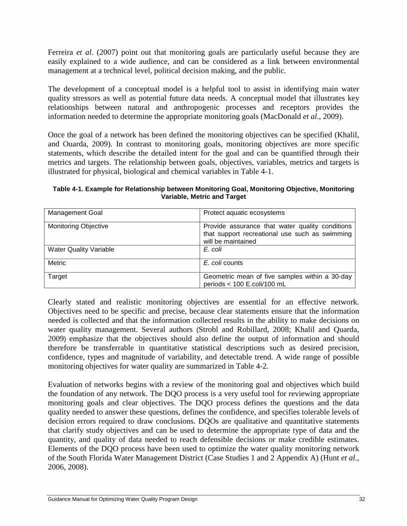
Ferreira et al. (2007) point out that monitoring goals are particularly useful because they are easily explained to a wide audience, and can be considered as a link between environmental management at a technical level, political decision making, and the public. The development of a conceptual model is a helpful tool to assist in identifying main water quality stressors as well as potential future data needs. A conceptual model that illustrates key relationships between natural and anthropogenic processes and receptors provides the information needed to determine the appropriate monitoring goals (MacDonald et al., 2009). Once the goal of a network has been defined the monitoring objectives can be specified (Khalil, and Ouarda, 2009). In contrast to monitoring goals, monitoring objectives are more specific statements, which describe the detailed intent for the goal and can be quantified through their metrics and targets. The relationship between goals, objectives, variables, metrics and targets is illustrated for physical, biological and chemical variables in Table 4-1.

Table 4-1. Example for Relationship between Monitoring Goal, Monitoring Objective, Monitoring Variable, Metric and Target

Management Goal Protect aquatic ecosystems

Monitoring Objective Provide assurance that water quality conditions that support recreational use such as swimming will be maintained

Water Quality Variable E. coli

Metric E. coli counts

Target Geometric mean of five samples within a 30-day periods < 100 E.coli/100 mL

Clearly stated and realistic monitoring objectives are essential for an effective network. Objectives need to be specific and precise, because clear statements ensure that the information needed is collected and that the information collected results in the ability to make decisions on water quality management. Several authors (Strobl and Robillard, 2008; Khalil and Quarda, 2009) emphasize that the objectives should also define the output of information and should therefore be transferrable in quantitative statistical descriptions such as desired precision, confidence, types and magnitude of variability, and detectable trend. A wide range of possible monitoring objectives for water quality are summarized in Table 4-2. Evaluation of networks begins with a review of the monitoring goal and objectives which build the foundation of any network. The DQO process is a very useful tool for reviewing appropriate monitoring goals and clear objectives. The DQO process defines the questions and the data quality needed to answer these questions, defines the confidence, and specifies tolerable levels of decision errors required to draw conclusions. DQOs are qualitative and quantitative statements that clarify study objectives and can be used to determine the appropriate type of data and the quantity, and quality of data needed to reach defensible decisions or make credible estimates. Elements of the DQO process have been used to optimize the water quality monitoring network of the South Florida Water Management District (Case Studies 1 and 2 Appendix A) (Hunt et al., 2006, 2008).


Table 4-2. Examples for Monitoring Objectives and Relationship to Time-Scale:

Monitoring Objectives Time Scale Identify spatial and temporal trends Long term and short term Operational status Short term Facilitate specific research questions Short term Delineation of water quality characteristics for water use Short term Assess compliance with water quality standards Short term or long term Evaluation of water quality control measures Short term and long term Estimate mass transport in rivers Short term and long term Facilitate impact assessment studies Short term Assess ecological status Long term Evaluate cumulative effects Short term or long term Questions that should be carefully considered during the review process to identify the usefulness of the collected data are summarized in Figure 4-1.

Figure 4-1. Toolbox for Optimizing Monitoring Goals and Objectives

Limitations and Risks in Defining Monitoring Goals and Objectives Common challenges associated with determining monitoring objectives are summarized by Khalil and Ouarda (2009) as follows: • selecting from multiple potential objectives • stating the objective • transforming objectives into statistical questions.

Defining objectives for monitoring networks with multiple objectives can be challenging, because multiple data users and a wide spectrum of contexts, including engineering, economic, social, and political, need to be considered. In the case of multiple objectives, an interactive design of single-purpose networks could be developed to meet individual objectives (Harmancioǧlu et al., 1999). This could result in combining some field or analytical efforts for more cost-efficiency, but the individual monitoring objectives need to remain distinct. Priorities need to be set if budgetary constraints exist. An example of the prioritization of objectives through a decision tree with guidelines for the selection and prioritizing of different types of monitoring programs is provided by Ferreira et al. (2007).

Step 1. Optimizing Monitoring Goals and Objectives

1. Determine if monitoring goals are clearly stated and realistic (conceptual model) 2. Determine if monitoring objectives are clearly identified in quantifiable measures 3. Provide flexibility to accommodate future objectives


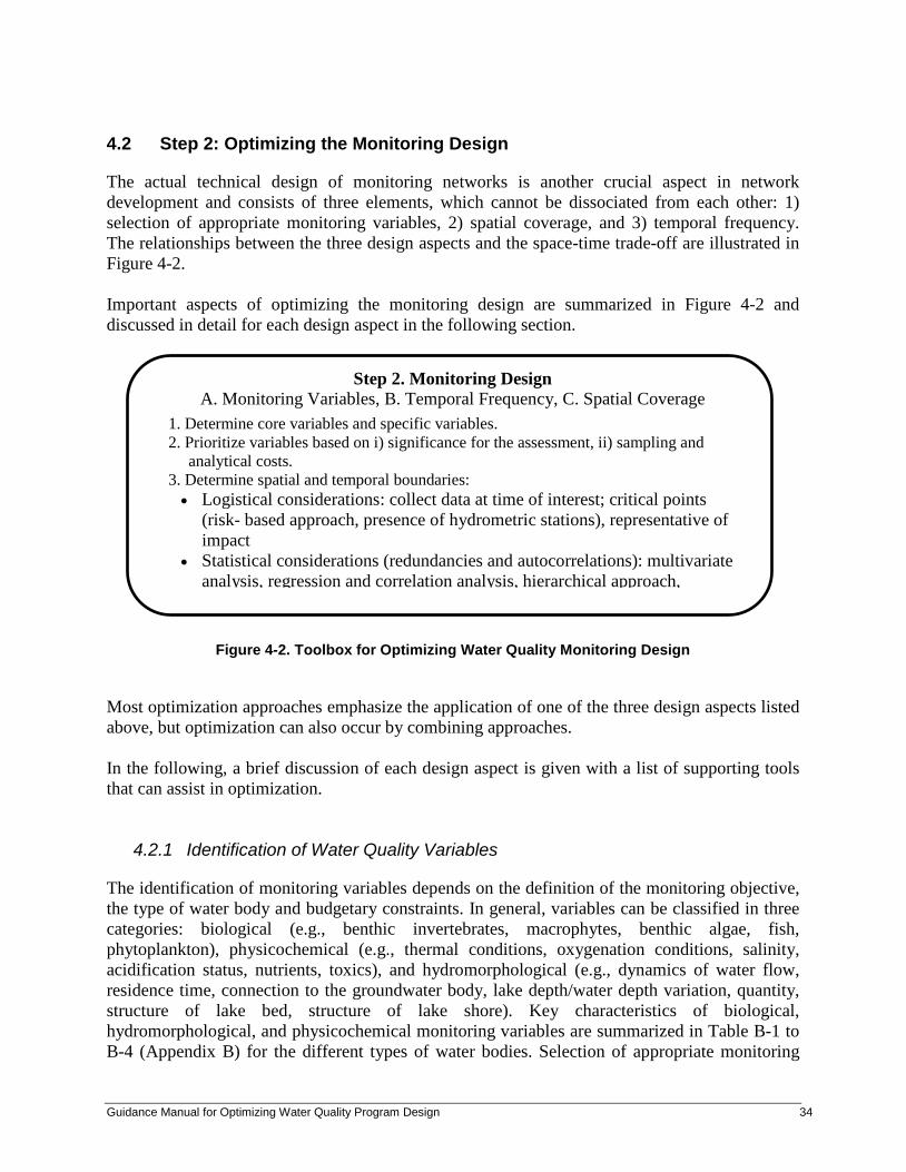
4.2 Step 2: Optimizing the Monitoring Design

The actual technical design of monitoring networks is another crucial aspect in network development and consists of three elements, which cannot be dissociated from each other: 1) selection of appropriate monitoring variables, 2) spatial coverage, and 3) temporal frequency. The relationships between the three design aspects and the space-time trade-off are illustrated in Figure 4-2. Important aspects of optimizing the monitoring design are summarized in Figure 4-2 and discussed in detail for each design aspect in the following section.

Figure 4-2. Toolbox for Optimizing Water Quality Monitoring Design

Most optimization approaches emphasize the application of one of the three design aspects listed above, but optimization can also occur by combining approaches. In the following, a brief discussion of each design aspect is given with a list of supporting tools that can assist in optimization.

4.2.1 Identification of Water Quality Variables

The identification of monitoring variables depends on the definition of the monitoring objective, the type of water body and budgetary constraints. In general, variables can be classified in three categories: biological (e.g., benthic invertebrates, macrophytes, benthic algae, fish, phytoplankton), physicochemical (e.g., thermal conditions, oxygenation conditions, salinity, acidification status, nutrients, toxics), and hydromorphological (e.g., dynamics of water flow, residence time, connection to the groundwater body, lake depth/water depth variation, quantity, structure of lake bed, structure of lake shore). Key characteristics of biological, hydromorphological, and physicochemical monitoring variables are summarized in Table B-1 to B-4 (Appendix B) for the different types of water bodies. Selection of appropriate monitoring

Step 2. Monitoring Design A. Monitoring Variables, B. Temporal Frequency, C. Spatial Coverage

1. Determine core variables and specific variables. 2. Prioritize variables based on i) significance for the assessment, ii) sampling and

analytical costs. 3. Determine spatial and temporal boundaries: • Logistical considerations: collect data at time of interest; critical points

(risk- based approach, presence of hydrometric stations), representative of impact

• Statistical considerations (redundancies and autocorrelations): multivariate analysis, regression and correlation analysis, hierarchical approach,


variables or the addition of new variables is complicated because many variables are interrelated. For example, chemical, physical, and biological changes in a stream are related to stream flow, so it is particularly important to understand the hydrology of the watershed and water body. Many non-point source particulate pollutants may be transported into waterways primarily during storm events or snowmelt periods that generate surface runoff. In some systems, these short-term, episodic conditions may be the most critical periods to monitor. The selection of water quality variables also needs to consider that contaminants behave differently in the aquatic environment and those matrices where the contaminant levels are expected to be significant (e.g., partitioning onto sediment and bioaccumulative contaminants such as PCBs). Biological variables (indicators) are very useful, because they reflect much longer time periods and provide more of an ecosystem perspective than chemical data. For example: • macroinvertebrates are the most relevant group used in stream assessments and for

hydropower generation • macrophytes are good indicators of changes in flow downstream of reservoirs, as well as for

the assessment of regulated lakes, because they are sensitive to water level • phytoplankton composition is an important indicator for nuisance algal blooms.

Monitoring of biological quality elements requires careful timing and appropriate taxonomic level to achieve adequate confidence and precision. Interpreting biological communities requires reliable data interpretation by experts and often a reference condition (e.g., minimally impacted site) to use as a benchmark. The selection of water quality variables also needs to consider costs such as analytical costs, costs related to specialized sampling and preservation techniques. Consideration should be given to reducing the number of water quality variables sampled without substantial loss of information (Strobl and Robillard, 2008). Qualitative and quantitative tools that assist in optimizing the selection of water quality variables are summarized in Table 4-3. Table 4-3. Qualitative and Quantitative Tools to Optimize the Selection of Water Quality Variables

in Water Quality Monitoring Design

Qualitative Tools Quantitative Tools

Identify core variables (background conditions) Correlation and regression methods

Identify specific variables (impact specific) Multivariate analysis (PCA)

Develop a priority list, include weighting factors (e.g., significance, analytical cost, temporal variability, ease of sampling)

Qualitative tools include establishing a priority list of parameters with core variables that reflect local geological and climatic background conditions (e.g., temperature, conductivity, pH, DO, ions, organic matter) and specific variables that relate to water use and anthropogenic stressors. A priority list of variables can be developed with weighting factors assigned based on


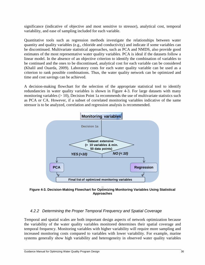
significance (indicative of objective and most sensitive to stressor), analytical cost, temporal variability, and ease of sampling included for each variable. Quantitative tools such as regression methods investigate the relationships between water quantity and quality variables (e.g., chloride and conductivity) and indicate if some variables can be discontinued. Multivariate statistical approaches, such as PCA and NMDS, also provide good estimates of the most representative water quality variables. PCA is ideal if the datasets follow a linear model. In the absence of an objective criterion to identify the combination of variables to be continued and the ones to be discontinued, analytical cost for each variable can be considered (Khalil and Ouarda, 2009). Laboratory costs for each water quality variable can be used as a criterion to rank possible combinations. Thus, the water quality network can be optimized and time and cost savings can be achieved. A decision-making flowchart for the selection of the appropriate statistical tool to identify redundancies in water quality variables is shown in Figure 4-3. For large datasets with many monitoring variables (> 10), Decision Point 1a recommends the use of multivariate statistics such as PCA or CA. However, if a subset of correlated monitoring variables indicative of the same stressor is to be analyzed, correlation and regression analysis is recommended.

_

Figure 4-3. Decision-Making Flowchart for Optimizing Monitoring Variables Using Statistical Approaches

4.2.2 Determining the Proper Temporal Frequency and Spatial Coverage

Temporal and spatial scales are both important design aspects of network optimization because the variability of the water quality variables monitored determines their spatial coverage and temporal frequency. Monitoring variables with higher variability will require more sampling and increased monitoring costs compared to variables with lower variability. For example, marine systems generally show high variability and heterogeneity in observed water quality variables

Final list of optimized monitoring variables

Dataset extensive (> 10 variables & min.

50 data points)

RegressionPCA

Monitoring variables

YES (>10) NO (< 10)

Decision 1a


and therefore there is a lower level of confidence in the data. This natural variability can be reduced by targeting the collection of data to specific seasons (i.e., measuring nutrient concentrations in near-shore and coastal waters during winter when nutrient uptake by biota is reduced) or by choosing equidistant time intervals between sampling events. Most statistical approaches for network optimization emphasize the determination of the proper resolution of the monitoring program in terms of the temporal frequency and spatial coverage of the project. The evaluation of temporal frequency and spatial coverage is discussed below. Determining and optimizing sampling frequency is a critical element of network optimization. The temporal frequency of a network is dependent on the spatial design and the monitoring variables observed. Temporal frequency affects costs; therefore, the sampling frequency should be adjusted so that sampling effort is minimal. Table B-5 (Appendix B) summarizes the minimum temporal frequencies required for different type of water bodies. The number of samples required to achieve a certain monitoring precision depends on the variability of the water quality variables measured. The greater the variation of the water quality variable, the greater the number of samples needed to obtain a statistically sound estimate. By increasing the number of samples collected, a reduction in the standard error of the mean value of the water quality variable can be achieved. Since the standard error of the mean is inversely proportional to the square root of the number of samples, an increase in the number of observations will consequently only lead to a small overall gain in results (Strobl and Robillard, 2008; Sanders et al., 1983). A commonly used method to determine sampling frequencies is the use of the confidence limits; the frequency selected is that which gives an estimate of the mean within a given confidence limit. The time scale has an important impact on monitoring activities, because sampling frequency is a major driver of costs. Qualitative and quantitative tools that assist in optimizing temporal frequency are summarized in Table 4-4.

Table 4-4. Qualitative and Quantitative Tools to Optimize Temporal Frequency in Water Quality Monitoring Design

Qualitative Tools Quantitative Tools Collect data at time of interest Confidence Interval Consider seasonal variability of the data Trend Analysis Geospatial tools

Qualitative tools to consider when determining temporal frequency are related to the selection of the time of interest such as periods of low flow or high flow, presence of benthic invertebrates, or seasonal timing (e.g., seasonal trends of pesticide application, impact of sewage, storm-water). Monitoring activities should be targeted to particular times of year to consider variability due to seasonal factors (e.g., sample for nutrients in marine waters in the winter when nutrient uptake by biota is at a minimum).


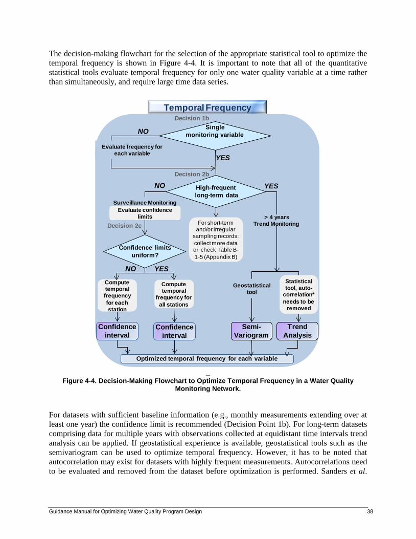
The decision-making flowchart for the selection of the appropriate statistical tool to optimize the temporal frequency is shown in Figure 4-4. It is important to note that all of the quantitative statistical tools evaluate temporal frequency for only one water quality variable at a time rather than simultaneously, and require large time data series.

_

Figure 4-4. Decision-Making Flowchart to Optimize Temporal Frequency in a Water Quality Monitoring Network.

For datasets with sufficient baseline information (e.g., monthly measurements extending over at least one year) the confidence limit is recommended (Decision Point 1b). For long-term datasets comprising data for multiple years with observations collected at equidistant time intervals trend analysis can be applied. If geostatistical experience is available, geostatistical tools such as the semivariogram can be used to optimize temporal frequency. However, it has to be noted that autocorrelation may exist for datasets with highly frequent measurements. Autocorrelations need to be evaluated and removed from the dataset before optimization is performed. Sanders et al.

NO

Decision 2c

Semi-Variogram

Geostatisticaltool

Trend Analysis

Statistical tool, auto-

correlation* needs to be

removed

> 4 yearsTrend Monitoring

Optimized temporal frequency for each variable

Confidence limitsuniform?

Confidence interval

YESNO

Confidence interval

Compute temporal

frequency for all stations

Compute temporal frequency for each station

YES

Decision 1b

Decision 2b

YES

For short-term and/or irregular

sampling records: collect more data or check Table B-1-5 (Appendix B)

Singlemonitoring variable

High-frequentlong-term data

Surveillance MonitoringEvaluate confidence

limits

Evaluate frequency for each variable

NO

Temporal Frequency


(1983) provide guidance on how to evaluate and remove autocorrelation from the variance of a dataset. Similar to the selection of temporal frequency, the selection of spatial coverage and the location of monitoring sites is an important aspect in monitoring network design. In the following subsections, different approaches are described that can be used to assess and optimize the selection of sampling locations. An understanding of the natural conditions is essential in water quality monitoring. Reference sites are important in trend and status monitoring because they help distinguish between background changes in water quality, or quantity, and changes attributable to the stressors. Caution must be taken to avoid interpreting natural changes as anthropogenic impacts. Reference sites also help to differentiate between ecological changes associated with seasonality or temporal dynamics. Qualitative and quantitative tools that assist in optimizing the selection of sites are summarized in Table 4-5.

Table 4-5. Qualitative and Quantitative Tools to Optimize Spatial Coverage in Water Quality Monitoring Design

Qualitative Tools Quantitative Tools

Logistical consideration Hierarchical approach

Stations need to be representative of the magnitude and impact of the sources as a whole

Regression analysis

Critical points such as location of contaminant sources, reference sites for climate change

Multivariate data analysis

Presence of hydrometric stations, gauging stations and required facilities

Geospatial tools

Risk-Based Approach (EC, 2012a)

Climate Change Adaptation (CCME, 2011a)


Qualitative tools include logistical considerations such as: • accessibility • representativeness: stations should represent the magnitude of the impact (e.g., locations

should be placed strategically to have accurate and reliable basin coverage; depth sampling for thermally stratified bodies such as lakes; select reference sites for monitoring long-term changes because anthropogenic activities can mask a trend)

• site-specific conditions (e.g., critical points, presence of zones of complete mixing, sensitive habitat)

• risk-based approach • suitability for climate change monitoring.

Most of the quantitative statistical tools aim to reduce the number of sample sites. The hierarchical approach is commonly used when no water quality data are available. Instead of using stream order, the hierarchical approach can be expanded and attributes such as flow or contaminant loadings could be included by assigning a combined weight. Multivariate analysis overcomes the drawback of considering only one variable at a time and considers all variables simultaneously. Classification techniques such as CA are very useful tools to identify water body groups characterized by hydrological, geomorphological, geographical and trophic conditions that form homogenous areas. However, unlike regression analysis, multivariate analysis does not allow for the reconstitution of information at discontinued locations. In addition, multivariate analysis assumes a linear relationship of the dataset; however, the relationships between chemical and ecological factors (such as abundance of species) may not always be linear. The decision-making flowchart for the selection of the appropriate statistical tool to identify spatial redundancies and identify monitoring sites that can be discontinued is shown in Figure 4-5. For large datasets with multiple variables Decision Point 1c recommends the use of multivariate techniques such as PCA or CA. If the dataset is limited and sites need to be relocated (Decision Point 2c) the stream order or hierarchical approach should be used to identify appropriate monitoring sites. Decision Point 3c indicates that stations can also be optimized based on a single monitoring variable using quantitative statistical approaches such as regression and correlation analyses or geostatistical tools. Geostatistical tools are very powerful for site selection because they allow for the consideration of cumulative effects. Khalil et al. (2011) stress that optimizing the spatial scale of a network should include water quality variables simultaneously with basin attributes such as climatic region, land use, geology, and the existence of point- or non-point sources. The author describes Artificial Neural Networks (ANN) as promising tools because they account for the nonlinear structure (data follow a nonlinear model) of the water quality data and perform nonlinear PCA and nonlinear CCA.


Figure 4-5. Decision-Making Flowchart to Optimize Spatial Coverage in a Water Quality Monitoring

Network.

4.2.3 Limitations and Risks in Defining Temporal Frequency and Spatial Coverage

It is challenging to determine the appropriate number of water quality variables, sample station coverage and the temporal frequency of a monitoring network, because these three aspects of the network are highly dependent on each other (Harmancioǧlu et al., 1999; Khalil et al., 2009). Different design scenarios have to be evaluated to decide whether to discontinue monitoring variables in favor of increasing spatial coverage and/or increasing the temporal frequency, or to keep more water quality variables while decreasing the spatial coverage and/or the temporal frequency. The final decision depends on the evaluation of cost reduction with respect to the different scenarios. Khalil et al. (2011) recommend economic analysis as the best tool to evaluate the space-time trade off, where the options are increasing sampling stations versus less frequent sampling or vice versa. Some sophisticated statistical approaches such as entropy analysis can be used to combine the spatial and temporal criteria to evaluate the space-time tradeoff and costs

Limited dataand/or need

for relocation

Hierarchical weighted approach

NO

Final list of optimized stations

Decision 2cYES

Develop criteria to identify stations that

could be discontinued (e.g. cost, variance)

PCA CA

Discrete Groups

Gradient

Multiple variables


YESYESDecision 3c

NO

Autocorrelation needs to be

removed

Regression

Decision 1c

Semi-Variogram

Geo-statistical

toolNO

Quantitative

Station relocation (watershed, attributes)

Spatial Coverage


can be included to select the best combination. Table B-6 (Appendix B) provides an overview on number of monitoring variables, temporal frequency and spatial coverage used for various monitoring goals. A common disadvantage of many of the statistical approaches is that they optimize networks around only one water quality objective at a time. Sanders et al. (1983) recommended that different temporal frequencies should be used for different objectives in order to maximize the information gain. This so-called proportional sampling (Khalil and Ouarda, 2009) consists of distributing a pre-determined number of samples among sample locations and water quality variables based on a given weight for each variable and location. Proportional sampling needs to be evaluated periodically to ensure that the number of samples collected meet the monitoring requirements (e.g., desired precision). 4.3 Step 3. Optimizing Data Collection and Data Quality

Monitoring design describes the selection of water quality variables, number and location of sample stations and temporal frequency and timing, and generally dictates the level of detail and the costs associated with data collection, sample analysis and data analysis. Temporal frequency has significant implications on sampling effort. Monitoring data can be obtained by sampling through direct field measurements, automatic samplers or remote sensing. The evaluation of networks should also consider the new emerging data collection technologies for water quality monitoring (Allan, 2006), because they can result in more effective and cost-efficient networks.

4.3.1 Data Collection, Data Quality Assurance Program

Data collection and analysis is often one of the more costly activities within a water quality monitoring network. As noted by Lovett et al. (2007), data consistency and data quality is one of the seven most important aspects of highly effective monitoring networks (see Section 2.7). Sampling methods should be rigorous, repeatable and well-documented and when possible, only accepted methods should be employed. Lovett et al. (2007) indicate that when methods change, an extended period should follow in which both the new and the old method are used in parallel. The authors also stress the importance of quality assurance programs to ensure the confidence of the data for future users. Every monitoring program requires a Quality Assurance Framework for data quality and a plan-do-check-improve model (Quality Management System) for continuous improvement. Some practical considerations for optimizing data collection and sample processing are summarized in Figure 4-6 and include logistical considerations: time required to reach the locations, maximum holding time between sample collection and sample analysis, cost effective sampling and analysis, coordination of data collection, and integration of volunteers.


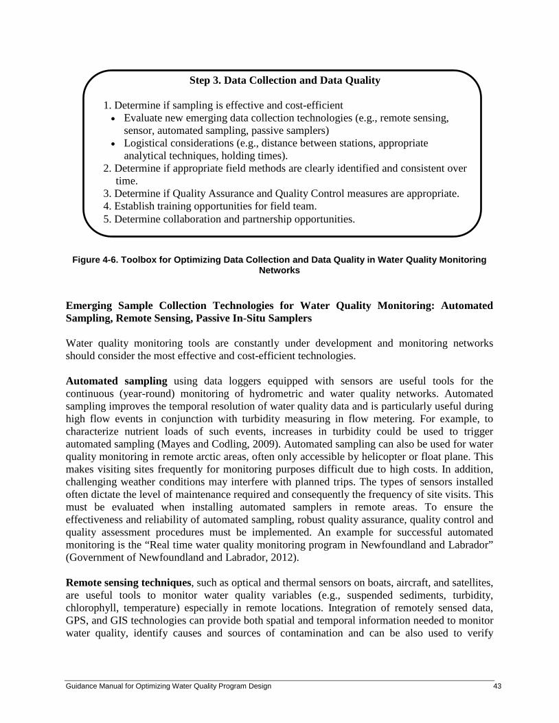
Figure 4-6. Toolbox for Optimizing Data Collection and Data Quality in Water Quality Monitoring Networks

Emerging Sample Collection Technologies for Water Quality Monitoring: Automated Sampling, Remote Sensing, Passive In-Situ Samplers Water quality monitoring tools are constantly under development and monitoring networks should consider the most effective and cost-efficient technologies. Automated sampling using data loggers equipped with sensors are useful tools for the continuous (year-round) monitoring of hydrometric and water quality networks. Automated sampling improves the temporal resolution of water quality data and is particularly useful during high flow events in conjunction with turbidity measuring in flow metering. For example, to characterize nutrient loads of such events, increases in turbidity could be used to trigger automated sampling (Mayes and Codling, 2009). Automated sampling can also be used for water quality monitoring in remote arctic areas, often only accessible by helicopter or float plane. This makes visiting sites frequently for monitoring purposes difficult due to high costs. In addition, challenging weather conditions may interfere with planned trips. The types of sensors installed often dictate the level of maintenance required and consequently the frequency of site visits. This must be evaluated when installing automated samplers in remote areas. To ensure the effectiveness and reliability of automated sampling, robust quality assurance, quality control and quality assessment procedures must be implemented. An example for successful automated monitoring is the “Real time water quality monitoring program in Newfoundland and Labrador” (Government of Newfoundland and Labrador, 2012). Remote sensing techniques, such as optical and thermal sensors on boats, aircraft, and satellites, are useful tools to monitor water quality variables (e.g., suspended sediments, turbidity, chlorophyll, temperature) especially in remote locations. Integration of remotely sensed data, GPS, and GIS technologies can provide both spatial and temporal information needed to monitor water quality, identify causes and sources of contamination and can be also used to verify

Step 3. Data Collection and Data Quality

1. Determine if sampling is effective and cost-efficient • Evaluate new emerging data collection technologies (e.g., remote sensing,

sensor, automated sampling, passive samplers) • Logistical considerations (e.g., distance between stations, appropriate

analytical techniques, holding times). 2. Determine if appropriate field methods are clearly identified and consistent over

time. 3. Determine if Quality Assurance and Quality Control measures are appropriate. 4. Establish training opportunities for field team. 5. Determine collaboration and partnership opportunities.


catchment pressures. Remote sensing techniques are often implemented to monitor harmful algal blooms in estuaries and coastal areas (Ferreira, 2007). Passive in-situ sampling devices are useful tools for monitoring long-term trends in water quality. They allow the screening of a large range of contaminants at very low concentrations, measurement of metal speciation and the identification of contaminant sources. Contaminant uptake in a passive sampler is based on accumulation in a receiving phase either with or without a diffusion-limiting membrane. The advantage of in situ passive samplers is that they integrate over time and measure a time-weighted average concentration. Passive in situ sampling devices may be especially relevant in water bodies with highly variable conditions or water bodies that are subject to seasonal anthropogenic impacts (Allan et al., 2006). 4.4 Step 4. Data Analysis, Interpretation and Evaluation

An important aspect in the evaluation and optimization of monitoring networks is an integrated approach to data management. This involves the harmonization among different steps of data management and different agencies and disciplines to ascertain availability and compatibility of the data. Robarts et al., (2008) indicate that modern monitoring programs are designed to be “effective keystone components of integrated water resources management”. The integration of data management systems and the development of compatible data and information systems is an important topic in network research because it allows scientists, and policy and decision makers at local, regional and Canada-wide levels to exchange information. Some practical considerations for optimizing data analysis, data management and network evaluation are summarized in Figure 4-7.

Figure 4-7. Toolbox for Optimizing Data Analysis and Data Management

Lovett et al., (2007) stress that data management, analysis and interpretation are key components for successful monitoring programs. Practical considerations for optimizing data management and analysis include integrated data management systems to ensure metadata with all relevant details of collection analysis and data reduction is archived; data should be shared and compared amongst a wide number of users (managers, scientists, public), and policies of confidentiality, data-ownership, data hold-back times should be established. Web-based services providing applications with user-friendly interfaces for complex analyses (e.g., Canadian Aquatic

Step 4. Data Analysis and Data Management

• Implement integrated approaches and standardized procedures for data management.

2. Determine appropriate data analysis methods. • Collaborate with academic community • Develop web-based user friendly interfaces for complex analyses.

3. Share data amongst a wide number of users (e.g., managers, scientists, public). 4. Evaluate monitoring network effectiveness and cost efficiency and optimize.


Biomonitoring Network and CABIN analysis tools, Government of Canada, 2012) can be developed. Water quality monitoring network design is an iterative procedure, and Step 4 also indicates the evaluation of an existing network for effectiveness and cost-efficiency to confirm that monitoring objectives and requirements (e.g., desired precision) are met. This review process will also allow appropriate adjustments to accommodate changing environmental data needs in water quality management to be made. Network evaluation should occur periodically, the USGS (1995) suggest every five years.

4.4.1 Limitations and Risks in Data Collection, Analysis and Management

The most common challenges in network optimization are associated with the integration of data management systems. This includes checking data compatibility such as sampling protocols, methods, names, and definitions. Adequate quality-assurance (QA) programs are needed to quantify the precision, accuracy, and integrity of environmental data to ensure that these data can be used for the appropriate application. These challenges can be overcome by developing and adopting common variable and data-element names, definitions, and formats. Also, standardized criteria to assess other methods could be made available so that even if different protocols were used to collect the data, there would be a way to compare the results and assess data compatibility. 4.5 Step 5. Optimizing Communicating and Interpretation

An essential and critical step in a successful monitoring program is the communication of monitoring results and the integration of information into decision-making processes. Reporting is imperative to ensure that data are fully understood, and to facilitate adjustments and modifications in response to new and emerging water issues, see Figure 2-1. The results of monitoring programs should be used to develop options for water resource management policies and effective management strategies (MacDonald et al., 2009). The translation of water quality variables into indices (e.g., CCME Water Quality Index, CCME, 2001a) or more general statements assists in the communication of water quality information to a broad audience. Other tools for improved communication between the monitoring community, policy makers and the public, include the development of web-based GIS approaches (USGS Sparrow Surface Water Quality Modeling, USGS, 2011), the establishment of reporting examples (e.g., Watershed Report Cards used by Conservation Authorities in Ontario, Conservation Ontario, 2009) and guidelines for publishing. Peer-reviewed publications establish and maintain the credibility of federal and provincial monitoring programs and scientists. Science published in journals can be translated into plain-language such that key findings are communicated to a broader audience.


Important practical considerations for optimizing the communication and interpretation element in water quality monitoring programs are summarized in Figure 4-8.

Figure 4-8. Toolbox for Optimizing Reporting and Communication

4.6 Collaboration and Partnership Opportunities

Monitoring efforts can benefit in many ways from linkages at the regional, provincial and/or federal level. Such benefits include: exchange of experience and data; coordinating sampling activities; network consolidation; data exchange; and situating water quality data within a broader geospatial context. Partnership monitoring can also be advantageous when considering costs. Water quality monitoring activities can be streamlined and coordinated between agencies and groups so that duplication of effort is avoided. The development of partnerships requires collaboration and information exchange with key partners and stakeholders such as governments, industries, academia and the public. Figure 4-9 shows the steps involved in water quality monitoring design and the relationships between water managers, academia and public. Collaboration and partnership approaches are fundamental to the successful management and sustainability of Canadian waters. They are increasingly important because water issues are becoming more complex, resources are tighter, and the demand for high-quality water continues to grow in order to support human activities and aquatic ecosystem needs. Several of these partnerships already exist including the Canada/Québec monitoring joint initiative in the St. Lawrence Action Plan that has been ongoing for many years, and the Canada/Québec Agreement on Water Quality Monitoring in Québec, signed in 2012 (Saint Lawrence Action Plan, 2013). The Province of Manitoba and the Government of Canada continue to lead a collaborative effort by many researchers from government, universities, and non-governmental organizations in comprehensively assessing the physical, chemical, and biological characteristics of Lake Winnipeg since intensive lake monitoring began in the late 1990s (State of Lake Winnipeg Report, 2011).

Step 5. Reporting and Communication

1. Transformation of data into information needed by audience: Data needs to be conveyed in various forms depending on the needs and preferences of the audience.

2. Improve conceptualization of data (e.g., geospatial tools) to ensure the variables measured are the most appropriate and that information is integrated into decision-making.

3. Establish reporting examples and guidelines for publishing.


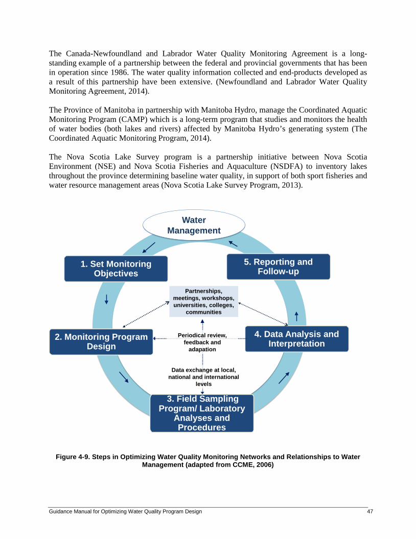
The Canada-Newfoundland and Labrador Water Quality Monitoring Agreement is a long-standing example of a partnership between the federal and provincial governments that has been in operation since 1986. The water quality information collected and end-products developed as a result of this partnership have been extensive. (Newfoundland and Labrador Water Quality Monitoring Agreement, 2014). The Province of Manitoba in partnership with Manitoba Hydro, manage the Coordinated Aquatic Monitoring Program (CAMP) which is a long-term program that studies and monitors the health of water bodies (both lakes and rivers) affected by Manitoba Hydro’s generating system (The Coordinated Aquatic Monitoring Program, 2014). The Nova Scotia Lake Survey program is a partnership initiative between Nova Scotia Environment (NSE) and Nova Scotia Fisheries and Aquaculture (NSDFA) to inventory lakes throughout the province determining baseline water quality, in support of both sport fisheries and water resource management areas (Nova Scotia Lake Survey Program, 2013).

Figure 4-9. Steps in Optimizing Water Quality Monitoring Networks and Relationships to Water Management (adapted from CCME, 2006)

1. Set MonitoringObjectives

3. Field SamplingProgram/ Laboratory

Analyses and Procedures

4. Data Analysis and Interpretation

5. Reporting and Follow-up

Water Management

Partnerships, meetings, workshops, universities, colleges,

communities

Periodical review, feedback and

adapation

Data exchange at local, national and international

levels

2. Monitoring ProgramDesign


4.6.1 Establishing Web-Portals

Open web services or the establishment of water quality monitoring portals that formalizes partnerships between multiple federal, provincial, territorial, local and academic entities brings together diverse expertise needed to develop collaborative, comparable, and cost-efficient approaches for monitoring and assessing water quality. An example is the National Water Quality Monitoring Council (USGS, 2013) in the United States that provides a national forum for coordination of comparable and scientifically defensible methods and strategies to improve water quality monitoring, assessment and reporting, and promotes partnerships to foster collaboration, advancement of science, and improved management within all elements of the water quality monitoring community. The forum also promotes technology transfer and training. A successful example for establishing a forum for exchange of ideas, data and science in water quality monitoring is provided by the Stream Monitoring and Research Team Ontario (SMART, Toronto and Region Conservation, 2013). They facilitate collaborative study design development that enables broader questions to be answered. This leads to better decision making capabilities for all participants. Consolidation of Networks A new trend in water quality monitoring has been to consolidate networks and to realize opportunities for efficiencies. The biggest challenge in network consolidation is the integration and compatibility of the data. This includes the definition of common data-elements, data quality, spatial and temporal attributes, water quality variables, and the incorporation of metadata. Integration of Volunteers The involvement of volunteers in water quality monitoring can be done during Step 3 (data collection). Opportunities should be provided to educate and train volunteers on laboratory, field, and quality-assurance methods and to encourage consistency in methods. Examples for successful community volunteering programs include community-based monitoring of lakes for algal blooms in Québec (Marty and Waller, 2012), and CABIN as a tool for teaching ecology in British Columbia (Duncan and Duncan, 2010). Environment Canada, in partnership with the Canadian Rivers Institute (CRI) at the University of New Brunswick (UNB), has developed an online training program of Canada-wide standardized protocols for aquatic biomonitoring. The full program consists of online learning modules followed by a field certification workshop. The training program is designed to accommodate a range of participants based on how CABIN will be applied. Those participants, who will be collecting samples or entering data, require less training than those who will be designing CABIN studies and using the suite of analytical tools that are available through the CABIN website. Once certified, CABIN partners gain access to a suite of web-accessible tools and resources such as a Canada-wide database of biological reference condition information, a data management system, analytical software and reporting tools.


5.0 PRIORITY SETTING IN SUCCESSFUL WATER QUALITY MONITORING PROGRAMS As noted by Lovett et al. (2007) there are many highly successful long-term monitoring programs that have contributed to environmental policy and scientific research. Ongoing review and refinement of the monitoring program ensures that water quality monitoring will continue to be relevant in supporting defensible decisions on the management of water resources. 5.1 Cost Benefit Analysis

Monitoring variables, as well as spatial coverage and temporal frequency of sampling, are the three main aspects of monitoring design. These dictate the costs of monitoring activities such as data collection, analysis and reporting. The development of a cost-efficient design is discussed in sections 4.1 to 4.3 and tools are presented to include costs and evaluate alternative monitoring configurations. Such tools include: prioritization of monitoring variables based on significance, analytical costs and equipment; spatial coverage based on logistical considerations such as accessibility and temporal frequencies through the evaluation of combined space/time designs. A cost-benefit analysis compares the costs of all alternate monitoring designs. Through the analysis the most resource-efficient design will be identified. Cost-savings can also be achieved by maximising the efficiency in data collection including logistical considerations in field-trip planning (e.g., number of staff deployed, duration of field work, type of transportation and equipment needed). Robarts et al. (2008) point out that data analysis is often an area where financial resources are underestimated. Since data analysis and network evaluation and optimization are closely linked sufficient resources need to be allocated to this step. Another important cost saving practice emphasized in the literature is to enhance and strengthen the forming of partnerships with the public, communities or other agencies that can be involved in monitoring activities such as data collection. This may be especially important for remote areas where the collection of a single sample can be very costly due to high travel costs. Partnerships with nearby communities can be very cost efficient and provide an economical benefit for community members. Such programs often require a training component. Cost-benefit analysis of monitoring networks evaluates the benefits of a network as a function of the data collected and their ability to satisfy the monitoring objectives. However, a cost-benefit analysis for a water quality monitoring network should also consider the environmental costs associated with adverse effects (remediation measures) expected if the monitoring is discontinued. Lovett et al. (2007) describe three examples of major environmental issues and compare the costs to improve the environmental issues with the cost of the monitoring efforts. Solutions to many environmental issues are expensive and technically challenging. The cost of monitoring is minuscule compared to the value of the monitored water resource, the financial benefits associated with environmental improvements and costs of policy implementation.


Quantification of these benefits is difficult, because it requires the consideration of non-market values (e.g., higher treatment costs to produce drinking water from polluted ground- or surface waters, financial benefits associated with improved aquatic health, beneficial impacts such as the contribution of wetlands and river banks to the regulation or capture of CO2 emissions and other air pollutants). 5.2 Flexibility of Monitoring Networks to Respond to New Environmental Issues

Monitoring objectives often change over time and new issues emerge (e.g., climate change, harmful algal blooms, pharmaceutical and personal care products, salinization). Therefore, monitoring networks have to be designed to be flexible enough to accommodate new and future objectives. As indicated by the feedback loop in Figure 4-9 that links the data analysis in Step 4 with the monitoring design aspect in Step 2, developing a monitoring network is an iterative process, and needs to be adaptive to changing data needs. An important, and often unconsidered, step in monitoring is the evaluation of the network design and output data during the data interpretation activity in Step 4. New insights gained since the last network evaluation lead to revisions and adjustments, and success or failures of previous management decisions can be determined so that necessary future adaptation can be made and implemented. Ongoing review and refinement of the monitoring program ensures that it will continue to be relevant in supporting defensible decisions on management of water resources. Monitoring networks need to be periodically evaluated and modified because of changing environmental issues and shifts in management priorities. For example, the impacts of climate change in Canada are expected to result in changes in lake levels and flow regimes that may impact aquatic health and translate to financial impacts to hydroelectric generation, irrigated agriculture, fisheries, and other industries (Bruce and Tin, 2006). Therefore, it is recommended that the impact of climate change on water quality should be assessed in water quality monitoring programs and the design of monitoring networks should be adjusted to incorporate this new goal. CCME has recently developed a reference document for non-specialist water managers to help Canadian federal, provincial and territorial governments determine the suitability of their water monitoring networks to provide the data needed to plan for and to adapt to a changing climate (CCME, 2011). The document describes proven and practical ways for jurisdictions to set priorities for water monitoring networks for climate change adaptation, and then evaluate the ability of these networks to provide the data needed to support climate change adaptation needs.


6.0 CONCLUSIONS 6.1 Summary of Proposed Approach for Optimization

Optimization of water quality monitoring programs occurs through a combination of different tools that each focus on a specific monitoring activity. Since monitoring objectives are different for each network, optimization approaches are not prescriptive and will vary for each monitoring design. There is no single best approach for effective monitoring and several approaches should be used to evaluate the efficiency and effectiveness of water quality monitoring networks. Figure 6-1 shows a step-by-step framework for optimizing water quality monitoring networks in Canada. A support toolbox based on systematic rational criteria is presented for each step. Figure 6-2 shows a decision flowchart for optimizing the three design aspects in water quality monitoring networks: water quality variables, temporal frequency and spatial coverage.


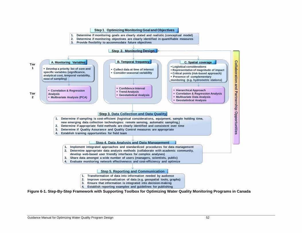
Figure 6-1. Step-By-Step Framework with Supporting Toolbox for Optimizing Water Quality Monitoring Programs in Canada

Tier 1

Tier 2

1. Determine if monitoring goals are clearly stated and realistic (conceptual model)2. Determine if monitoring objectives are clearly identified in quantifiable measures3. Provide flexibility to accommodate future objectives

Step 1. Optimizing Monitoring Goal and Objectives

Step 2. Monitoring Design

Correlation & Regression Analysis Multivariate Analysis (PCA)

Hierarchical Approach Correlation & Regression Analysis Multivariate Data Analysis Geostatistical Analysis

Develop a priority list of core and specific variables (significance, analytical cost, temporal variability, ease of sampling)

Logistical considerations Representative of magnitude of impact Critical points (risk-based approach) Presence of complementary monitoring (e.g. hydrometric stations)

Collect data at time of interest Consider seasonal variability

C. Spatial coverageA. Monitoring Variables B. Temporal frequency

Confidence Interval Trend Analysis Geostatistical Analysis

Step 4. Data Analysis and Data Management

Step 3. Data Collection and Data Quality1. Determine if sampling is cost-efficient (logistical considerations, equipment, sample holding time,

new emerging data collection technologies: remote sensing, automatic sampling,) 2. Determine if appropriate field methods are clearly identified and consistent over time3. Determine if Quality Assurance and Quality Control measures are appropriate4. Establish training opportunities for field team

1. Implement integrated approaches and standardized procedures for data management2. Determine appropriate data analysis methods (collaborate with academic community,

develop web-based user friendly interfaces for complex analyses)3. Share data amongst a wide number of users (managers, scientists, public)4. Evaluate monitoring network effectiveness and cost-efficiency and optimize

Collaboration and Partnership O

pportunities

Step 5. Reporting and Communication1. Transformation of data into information needed by audience2. Improve conceptualization of data (e.g. geospatial tools, graphs)3. Ensure that information is integrated into decision-making 4. Establish reporting examples and guidelines for publishing


Figure 6-1. Decision-Making Flowchart for Optimizing Water Quality Monitoring Design Using Quantitative Statistical Tools (Tier 2)

Space/Time tradeoff:Perform cost benefit analysis to select best combination of

temporal frequency and spatial coverage

Examine available monitoring data (descriptive statistics)

Limited dataand/or need

for relocation

Hierarchical weighted approach

NO

Final list of optimized stations

Decision 2cYES

Develop criteria to identify stations that

could be discontinued (e.g. cost, variance)

PCA CA

Discrete Groups

Gradient

Multiple variables


YESYESDecision 3c

NO

Autocorrelation* needs to be

removed

Regression

Decision 1c

Semi-Variogram

Geo-statistical

toolNO

Quantitative

Station relocation (watershed, attributes)

NO

Decision 2c

Semi-Variogram

Geostatisticaltool

Trend Analysis

Statistical tool, auto-

correlation* needs to be

removed

> 4 yearsTrend Monitoring

Optimized temporal frequency for each variable

Confidence limitsuniform?

Confidence interval

YESNO

Confidence interval

Compute temporal

frequency for all stations

Compute temporal frequency for each station

YES

Decision 1b

Decision 2b

YES

For short-term and/or irregular

sampling records: collect more data or check Table B-1-5 (Appendix B)

Singlemonitoring variable

High-frequentlong-term data

Surveillance Monitoring Evaluate confidence

limits

Evaluate frequency for each variable

NO

Final list of optimized monitoring variables

Dataset extensive (> 10 variables & min.

50 data points)

RegressionPCA

Monitoring variables

YES (>10) NO (< 10)

Decision 1a

“Optimization” programsEntropy*

ANN*Dynamic Programming*

Bayesian analysis*

Spatio/Temporal Analysis

*complex statistical analysisuseful for optimization of largedata-rich networks

Temporal Frequency Spatial Coverage


The first step starts with the evaluation of the efficiency of the network in terms of data usefulness using the DQO process. Optimization tools for the technical design aspects in water quality monitoring are described in Step 2 and include two tiers: • Tier 1: qualitative tools based on systematic rational criteria, and • Tier 2: quantitative tools based on statistical approaches such as correlation and regression

analysis, confidence interval, geostatistics, multivariate analysis.

A decision-making flowchart to select approriate statistical tools for the Tier 2 approach is summarized in Figure 6-2

Common challenges in network design are the technical aspects related to determining the appropriate number of water quality variables, sample station locations and the temporal frequency of sampling, because these three aspects are highly dependent on each other. The qualitative tools within Step 2 are useful tools that can be applied to both longer-term and shorter-term monitoring networks. Careful consideration needs to be given to the evaluation of temporal frequencies, because they are often the major driving costs in the operation of a monitoring network. The decision whether to increase spatial coverage and decrease temporal frequency or decrease spatial frequency and increase temporal frequency depends on the evaluation of cost reduction with respect to decreases in space and time frequencies. Long-term trend monitoring generally requires a higher temporal frequency. Shorter-term monitoring programs may need to focus on optimizing spatial frequencies, and in terms of the temporal scale, seasonal aspects need to be considered as well as the selection of the proper time of interest (e.g., surface runoff, pesticide application, periods of low-flow). Many of the qualitative tools address only one specific water quality variable at a time and result in optimization of one of the monitoring objectives. Proportional sampling techniques can be used which distribute a pre-identified number of samples among monitoring locations for multiple objectives (Khalil and Quarda, 2009). The quantitative tools (Tier 2) should be used for optimization of costly networks with large datasets (high number of stations, high temporal frequency or complex, expensive laboratory costs) or for assessing variables, spatial and temporal redundancies during network consolidation. The quantitative tools (Tier 2) can also include more complex statistical approaches such as entropy analysis that can be used to combine spatial and temporal criteria to evaluate the space–time trade-off and costs can be included to select the best combination. Optimization Steps 3 to 5 provide a number of additional qualitative tools that support effectiveness and cost-efficiency in water quality monitoring networks. An important consideration in network optimization is the opportunity to collaborate and integrate networks.

Guidance Manual for Optimizing Water Quality Monitoring Program Design 54

7.0 References Allan I.L., Mills G.A., Vrana B., Knutsson J., Holmberg A., Guigues N., Laschi S., Fouillac A.M. and R.

Greenwood (2006). Strategic monitoring for the European Water Framework Directive. In Trends in Analytical Chemistry, 25 (7), pp. 604-715.

ASTWMO (Association of State and Territorial Solid Waste Management Officials) (2009): Framework for Long-Term Monitoring of Hazardous Substances at Sediment Sites.

Beveridge D., St-Hilaire A., Ouarda TB, Khalil B., Conly F.M., Wassenaar L.I., and E. Ritson-Bennett (2012): A geostatistical approach to optimize water quality monitoring networks in large lakes. Application to Lake Winnipeg. In Journal of Great Lakes Research 38, pp. 174–182.

Bruce, J. and T. Tin (2006): Implications of a 2°C global temperature rise on Canada’s water resources. http://tidescanada.org/wp-content/uploads/files/papers/sagereport_nov0106.pdf.

CCME (Canadian Council of Ministers of the Environment) (2001a): CCME Water Quality Index, Technical Report. 13 pp.

CCME (Canadian Council of Ministers of the Environment) (2001b): CCME Water Quality Index, User's Manual. 5 pp.

CCME (Canadian Council of Ministers of the Environment) (2006): A Canada-Wide Framework for Water Quality Monitoring. 29 pp.

CCME (Canadian Council of Ministers of the Environment) (2011): Selected tools to evaluate water monitoring networks for climate change adaptation. 164 pp.

Cetinkaya C.P. and N.B. Harmancioǧlu (2012): Assessment of Water Quality Sampling Sites by a Dynamic Programming Approach. In Journal of Hydrologic Engineering 17, pp. 305–317.

Chapman D. (1996): Water Quality Assessments. A Guide to the Use of Biota, Sediments and Water in Environmental Monitoring. 2nd edition. Chapman & Hall, London.

Clark, M.J.R, MacDonald D.D., Whitfield P.H. and M.P. Wong (2010): Designing monitoring programs for water quality based on experience in Canada II. Characterization of problems and data-quality objectives. In Trends in Analytical Chemistry 29 (5), pp. 385–398.

Clarke, K.R. and R.M. Warwick (2001): Change in marine communities: an approach to statistical analysis and interpretation 2nd edition., Plymouth Marine Laboratory, UK.

Conservation Ontario (2009). Watershed Reporting. Retrieved from http://dev.conservationontario.ca/watershed_monitoring/index.html.

Coordinated Aquatic Monitoring Program (2013). Retrieved from http://campmb.com/ Dowdall, M., Gerland, S., Karcher, M., Gwynn, J.P., Rudjord A.L. and A. K. Kolstad (2005): Optimisation of

Sampling for the temporal monitoring of technetium-99 in the Arctic marine environment, J. Environ. Radioact., 2005, 84, 111–130

Duncan J. and L. Duncan. (2010). Citizen Science and Cabin. Columbia Basin Water Quality Network, Kimberley, BC. National CABIN Science Forum Proceedings, Vancouver Convention Centre.

EC (European Communities) (2003): Common Implementation Strategy for the water framework directive (2000/60/EC), Guidance Document No 7. Monitoring under the Water Framework Directive. Policy Summary to Guidance No. 7. With assistance of Produced by Working Group 2.7 - Monitoring. 160 pp.

Environmental Protection Agency (EPA) (2006). Water Framework Directive Monitoring Programme. Prepared to meet the requirements of the EU Water Framework Directive (2000/60/EC) and National Regulations implementing the Water Framework Directive, Published by the Environmental Protection Agency, Ireland, Version 1.0.

Environment Canada (EC) (2012a): A Risk-based Approach to Evaluating Surface Water Quality Sites in the Federal Water Quality Monitoring Network.

Environment Canada (EC) (2012b): Guidance Document on the sampling and preparation of contaminated soil for use in biological testing.

Ferreira J.G.; Vale C., Soares C.V., Salas F., Stacey P.E. and S.B. Bricker (2007): Monitoring of coastal and transitional waters under the E.U. Water Framework Directive. In Environ Monit Assess 135 (1-3), pp. 195–216.

Global Environment Monitoring System Water Programme (GEMS) 2005. United Nations Envronment Programme Global Environment Monitoring. Operational Guide for Data Submission

Government of Canada (2012). Environment Canada - Canadian Aquatic Biomonitoring Network (CABIN). Retrieved from http://www.ec.gc.ca/rcba-cabin/


http://tidescanada.org/wp-content/uploads/files/papers/sagereport_nov0106.pdf

http://campmb.com/

http://www.ec.gc.ca/rcba-cabin/

Government of Newfoundland (2012). Real time Water Quality Monitoring Program. Retrieved from http://www.env.gov.nl.ca/env/waterres/rti/rtwq/index.html

Harmancioǧlu N., Fistikoglu O., Ozkul S.D., Singh V.P. and M.N. Alpaslan (1999): Water quality monitoring network design. Water Science and Technology. Dordrecht/Boston/London: Kluwer Academic Publisher (33).

Horton R.E. (1945): Erosional Development of Streams. Geological Society Am. Bull., 56, 281–283. Hunt C.D., Field J., Rust S. and P. Burke. (2006): Surface Water Quality Monitoring Network Optimization.

Comprehensive Report to the South Florida Water Management District. 87 pp. Hunt C.D., Steven W. Rust and L. Sinnott (2008): Application of statistical modeling to optimize a coastal water

quality monitoring program. In Environmental Monitoring and Assessment 137, pp. 505-522. Khalil B. and Ouarda T.B. (2009): Statistical approaches used to assess and redesign surface water-quality

monitoring networks. In Journal of Environmental Monitoring 11 (11), pp. 1915–1929. Khalil B., Ouarda T.B., M.J St-Hilaire A. Chebana F. (2010): A statistical approach for the rationalization of water

quality indicators in surface water quality monitoring networks. In Journal of Hydrology 386 (1-4), pp. 173–185.

Khalil, B.; Ouarda T. B., and M. J. St-Hilaire (2011): A statistical approach for the assessment and redesign of the Nile Delta drainage system water-quality-monitoring locations. In Journal of Environmental Monitoring 13 (8), p. 2910.

Krige, D.G. (1951). A ststistical approach to seome basic mine valuation problems in the Witwatersrand. Journal of Chemical, Mettalurgical and Mining Society of South Africa 52, 119. Laing, T. (2001): Developing Long-term Monitoring Programs that Lead to Site Closure for FCSAP Aquatic

Contaminated Sites: State of Science Review and Technical Guide. Lettenmaier D.P. (1976): Detection of trends in water quality data from records with dependent observations, Water

Resource Research 12, pp. 1037–1046. Loftis, J.C. and R. C. Ward (1980): Water Quality Monitoring Some Practical Sampling Frequency Considerations.

In Environmental Management 4(6), pp. 521–526. Lovett G. M., Burns D.A. and C.T. Driscoll (2007): Who needs environmental monitoring? In Frontiers in Ecology

and the Environment 5, pp. 253–260. MacDonald D.D., Malcolm J.R C.,Whitfield P. H. and Wong M. P. (2009): Designing monitoring programs for

water quality based on experience in Canada I. Theory and framework. In Trends in Analytical Chemistry 28 (2), pp. 204–213.

Marty J. and M. Waller (2012). Algae and Algae Monitoring, Presentation at Stream Monitoring, Assessment & Research Team Eastern Region (SMARTER) Fall Meeting 2012 on November 1st 2012 at Rideau Valley Conservation Authority Office.

Matheron, G., (1963). Principles of geostatistics. Economic Geology 58, 1246e1266 Mayes E. and Codling (2009). Water Framework Directive and Related Monitoring Programmes. In Biology and

Environment: Proceedings of the Royal Irish Academy 109B, pp. 321-344. Mishra A.K and P. Coulibaly. (2010): Hydrometric network evaluation for Canadian watersheds. In Journal of

Hydrology 380 (3-4), pp. 420–437. Newfoundland and Labrador Water Quality Monitoring Agreement (2014). Retrieved from

http://www.env.gov.nl.ca/env/waterres/quality/background/agreement.html#8 Nova Scotia Lake Survey Program (2013). Retrieved from http://novascotia.ca/fish/programs-and-services/industry-

support-services/inland-fisheries/lake-inventory-maps/ Ozkul S., Harmancioǧlu N.B. and V.P. Singh. (2000): Entropy-Based Assessment of Water Quality Monitoring

Networks. In Journal of Hydrologic Engineering 5 (1), pp. 90–100. Robarts R., Barker S.J. and S. Evans (2008): Water Quality Monitoring Assessment: Current Status and Future

Needs. Proceedings of Taal 2007: The 12th World Lake Conference. Sanders T.G., Ward R.C., Loftis J.C., Steele T.D., Adrian D.D. and V. Yevjevich (1983): Design of Networks for

Monitoring Water Quality. Water Resources Publications, Littleton, Colorado, pp. 328. Saint Lawrence Action Plan (2013). Integrated Management of the Saint Lawrence. Retrieved from

http://planstlaurent.qc.ca/en/state_monitoring.html Schindler, D. W. (2009): Lakes as sentinels and integrators for the effects of climate change on watersheds, airsheds,

and landscapes. In Limnology and Oceanography. 54, pp. 2349–2358. Schulze F.H. and F.H. Bouma. (2001): Use of artificial neural networks in integrated water management.

Proceedings Monitoring Tailor-made III, pp. 333-342. Shannon C.E. (1948): A mathematical theory of communication. In Bell System Technical Journal, 27, pp. 397–423. Sharp, W.E (1971): A topologically optimum water - sampling plan for river and streams. In Water Resources

Research 6(3), pp. 1641–1646.


http://www.env.gov.nl.ca/env/waterres/rti/rtwq/index.html

http://www.env.gov.nl.ca/env/waterres/quality/background/agreement.html%238

http://planstlaurent.qc.ca/en/state_monitoring.html

State of Lake Winnipeg Report (2011). State of Lake Winnipeg Report. Retrieved from http://www.gov.mb.ca/conservation/waterstewardship/water_quality/state_lk_winnipeg_report/index.html

Strobl R. O. and P.D. Robillard. (2008): Network Design for Water Quality Monitoring of Surface Freshwaters: A Review. In Journal of Environmental Management 87 (1-3), pp. 639–648.

Strobl R. O., Robillard P.D., Shannon R.D., Day R.L. and A.J. McDonnell (2006): A Water Quality Monitoring Network Design Methodology for the Selection of Critical Sampling Points: Part I. In Environmental Monitoring and Assessment 112 (1-3), pp. 137–158.

Swertz, O.C, Laane R.W.P and K.J.M. Kramer (1997): An assessment of water quality monitoring in the Dutch coastal zone: Needs, Aims and Optimization. Monitoring Tailor-made I.

Tabachnick B.G. and L.S. Fidell. (1996): Using Multivariate Statistics. Allyn and Bacon, Boston, London, pp. 879. Toronto and Region Conservation (2013). Southern Ontario Stream Monitoring and Research Team (SOSMART).

Retrieved from http://www.trca.on.ca/the-living-city/monitoring/southern-ontario-stream-monitoring-research-team.dot.

USEPA (United States Environmental Protection Agency) (2006a): Guidance on Systematic Planning Using the Data Quality Objectives Process. EPA QA/G-4. 121 pp.

USEPA (United States Environmental Protection Agency) (2006b): Data Quality Assessment: Statistical Methods for Practitioners. EPA QA/G-9S. 190 pp.

USGS (US Geological Survey) (2013): About the National Water Quality Monitoring Council. Retrieved from http://acwi.gov/monitoring/about_the_council.html.

USGS (US Geological Survey) (2011): USGS Sparrow Surface Water Quality Modeling, retrieved from http://water.usgs.gov/nawqa/sparrow/

USGS (US Geological Survey (Ed.) (1995): The Strategy for Improving Water-Quality Monitoring in the United States. Book Final Report of the Intergovernmental Task Force on Monitoring Water Quality. Open File Report 95-742. 161 pp.

WMO (World Meteorological Organization) (1994): Guide to Hydrological Practice, WMO-No. 168, WMO Geneva, pp 770.


http://www.gov.mb.ca/conservation/waterstewardship/water_quality/state_lk_winnipeg_report/index.html

http://www.trca.on.ca/the-living-city/monitoring/southern-ontario-stream-monitoring-research-team.dot

http://www.trca.on.ca/the-living-city/monitoring/southern-ontario-stream-monitoring-research-team.dot

http://acwi.gov/monitoring/about_the_council.html

http://water.usgs.gov/nawqa/sparrow/

Appendix A - Case Studies


Case Study 1. South Florida Water Management District (Hunt et al., 2006), Data Quality Objectives

Data Quality Objectives: Spatial coverage, temporal frequency and indicator redundancy

Optimization Approach

• The South Florida Water Management District (SFWMD) has a large and expanding surface water level-monitoring network (~ 2000 stations) with 35,000 sampling events each year for various water bodies including lakes and streams.

• Optimization focused on: • Monitoring objectives • Station redundancy: Spearman Rank correlation • Water quality indicators per station: PCA • Temporal frequency: Trend power analysis (Seasonal Kendall Tau trend

analysis) • Procedure, confidence intervals) • Cost/benefit analysis (temporal frequency and logistics)

Location • South Florida, USA

Study Objective • To use scientifically defensible methods and robust statistical analyses to evaluate and optimize water quality monitoring programs to ensure cost effective monitoring. To determine if the data were sufficient to support trend evaluation and detection of changes in trends

Monitoring Objective • Determine general water quality; monitoring is driven by a diverse set of mandates (i.e., laws, permits, agreements, etc.) and objectives

Data used in case study

• Large dataset, over 1500 active monitoring sites, network consisted of several individual monitoring projects

• Data from 1992 through 2003 • Projects were optimized using up to five key water quality parameters.

Software • SAS (http://www.sas.com/) • (SAS code and step by step instructions provided in Rust 2005 (see Hunt

et al., 2006, Attachment 1) Expertise • Statistical skills to perform power analysis procedure (Monte Carlo based

power analysis procedure) and Seasonal Kendalls’ Tau trend analysis. Applicable Scenario • Large scale; long-term statistical results suggest that at least 10 years of

data are required to detect trends Findings/ Recommendations

• Expanding from concentration based data to loading which incorporated flow data

• Maximizing the use of auto-samplers where loading data is a key end use (reducing effort on back up samples)

• More precisely defining the level of change and period over which change should be detected so as to improve further temporal optimizations

• High temporal variability and fixed seasonal effects along with the high degree of autocorrelation limits ability to obtain truly independent samples.

Lessons Learned • Modification of temporal frequency; revisions in the stations sampled (remove, relocate, add); and, changes in the parameters measured

• Strong autocorrelation was determined • Clearly defining the data end uses so that the monitoring program can be

designed to collect the appropriate information • Expanding the optimization for several projects from concentration • Field-related costs ( > 75%) from staff time and transportation should also

be considered in optimization (Redfield et al., 2008).


http://www.sas.com/

Case Study 2. Massachusetts Bay (Hunt et al., 2008), Data Quality Objectives

Data Quality Objectives: station redundancy; spatial coverage and temporal frequency

Optimization Approach • Statistical Tools (correlation analysis, analysis of seasonal patterns, modeling tools)

• The long-term monitoring plan implemented by the Massachusetts Water Resource Authority consists of an intense spatial and temporal water quality measurement program

• Different statistical models were employed for the survey averages depending on whether or not there was evidence of a seasonal pattern in the data

• Optimization used model survey average readings to identify temporal fixed effects, model survey-average-corrected individual station readings to identify spatial fixed effects, corrected the individual station readings for temporal and spatial fixed effects and derived a correlation model for the corrected data, and applied the correlation model to characterize the correlation of annual average readings from reduced monitoring programs with true parameter levels.

Location • Boston Harbour and Massachusetts Bay

Study Objective • To address the potential sampling redundancies in the measuring program and evaluate the impact of reduced levels in monitoring on the ability to make waste quality decisions was assessed.

Monitoring Objective • Determine water quality using physic-chemical variables and biota samples.


• Data from 1992 – 2003 • Two parameters: DO and chlorophyll.

Software SAS PROC procedure MIXED

Expertise Basic statistical knowledge

Applicable Scenario • Marine coastal waters, large scale, long-term data. Findings/ Recommendations

Analysis led to recommendations for a substantially lower monitoring effort with minimal loss of information. Supported an annual budget savings of approximately $183,000. Most savings was from decreasing temporal frequencies.

Lessons Learned Reductions in the number of sampling stations were found less detrimental to the quality of the data for annual decision-making than reductions in the number of surveys per year. Model was not able to capture seasonal spring and fall bloom in chlorophyll a.


Case Study 3. Dutch Coastal Zones, Netherlands (Swertz et al., 1997), Confidence Intervals, Trend Analysis

Confidence Interval, Trend analysis: Temporal frequency

Optimization Approach Statistical analysis using confidence intervals, trend analysis, correlation analysis, and analysis of variance. Criteria used: detectable trends of 50% within ten years.

Location Dutch marine waters

Study Objective Statistical study to provide recommendations for more efficient monitoring. Investigating whether monitoring sites were superfluous by way of a correlation study: • Comparing different sampling media (water, sediment, biota) • Optimizing the number of observations • Estimating components of variation using analysis of variance • Investigating correlation of measured variables.

Monitoring Objective • General water quality.


• Data from 1988-1994 • Marine waters divided into 11 water systems based on chemical and

hydrological characteristics. Software Statistical software

Expertise Basic data management and statistical skills

Applicable Scenario Marine, coastal waters, large scale, long-term data, different matrices (water, sediment, biota)

Findings • Station reduction from 76 to 32 • Recommended increase in pesticide analyses • Recommended shift in sampling media: less water samples, more

sediment samples • Observations of dissolved substances at adjacent sites (several

kilometers apart) could be used to predict each other with an accuracy >90%

• Monitoring at intervals of less than a month provided redundant data in marine water areas

• Clear criteria for starting and stopping monitoring activities were developed.

Lessons Learned The number of monitoring sites was reduced from 75 to 32. Fewer heavy metal analyses since concentrations of these substances frequently met the targets. The program has been rendered more effective, but no change in analytical costs were achieved.


Case Study 4. Gediz River, Turkey (Harmancioǧlu et al., 1999), Hierarchical Structure

Hierarchical Structure (Stream Order Approach): Station relocation and spatial coverage


• Two approaches for determining macrolocations • 1) allocation by the number of contributing tributaries and • 2) allocation by the number of pollutant discharges. • • The first approach systematically locates sampling sites so as to divide the

river network into sections which are equal with respect to the number of contributing tributaries. Stream ordering is the first step in the method, where each exterior tributary is considered to be of first order. Ordering is carried out along the entire river such that a section of the river formed by the intersection of two upstream tributaries will have an order described as the sum of the orders of the intersecting streams. Next, the river is divided into hierarchical sampling reaches.

• • In the second approach, the same procedure is used by cumulatively

numbering the discharges from polluting sources as if they are exterior tributaries. Consequently, the sampling locations are determined as functions of populations and industrial activities.

Location • Gediz River, Turkey

Study Objective • Evaluate monitoring locations in a basin on the basis of drainage characteristics and effluent discharges to the river.

Monitoring Objective • Detect, isolate and identify a source of pollution • Assess basin-wide changes in water quality


• Stream flows from 24 stations; water quality parameters from 14 sampling stations

Software • Basic tabulation and statistical software

Expertise • Basic data management and statistical skills

Applicable Scenario • Large or small scale studies

Findings • Allocation of sampling sites on the basis of the number of contributing tributaries or on the number of outfalls logically divides the basin into equal parts with respect to tributaries and outfalls

• The locations of existing stations do not correspond to the new sites, primarily because the former have been established as project-orientated observations sites

• The crucial factor in the approach based on ordering of tributaries is the selection of tributaries to be considered. This selection has a subjective aspect which, nevertheless, may be minimized by judging on the basis of mean minimum flow, minimum area of recharge basin, or other similar quantitative criteria.

Lessons Learned • The design method is not completely objective; however, it does provide a systematic and logical selection of representative sites. It is also fairly flexible so that one may account for local factors to change the locations some distance upstream or downstream without upsetting the macrolocation

• The procedure has to be justified by analyzing the trade-offs between spatial coverage of stations and the temporal frequencies plus the variables to be observed.


Case Study 5. Watershed in Pennsylvania (Strobl et al., 2006a, b), Geospatial Analysis

Geospatial tools: spatial coverage


• Describes the Critical Sampling Points (CSP) method to resolve the spatial component of the design of a water quality monitoring network

• Critical Sampling Points (CSP) methodology translated into a model, called Water Quality Monitoring Station Analysis (WQMSA) that incorporates GIS for spatial analysis and data manipulation purposes, a hydrologic/water quality simulation model for estimating total phosphorous (TP) loads, and an artificial intelligence technology for improved input data representation

• A computed overall potential stream pollution index (PSPI) is used to ultimately rank each stream reach with respect to other stream reaches in the watershed according to its potential TP load

• It includes an economic as well as logistical component in order to approximate the number of sampling points required for a given budget and to only consider the logistically accessible stream reaches in the analysis, respectively.

Location Small Pennsylvanian watershed

Study Objective • To develop with minimal data a practical and scientifically-based design methodology for designating critical water quality monitoring network sampling points within small agricultural-forested watersheds with respect to TP.

Monitoring Objective Measuring total phosphorous loads


• Validity of the CSP methodology was tested on a small watershed for which TP data from a number of single storm events were available for various sampling points within the water shed

• The CSP methodology requires the watershed be discretized into square cells. The cell size will depend upon the detail of data as well as computational resources available

• Model input data include a number of hydrologic, topographic, soils, vegetative, and land use factors

• The user of the model is asked to weigh the importance of each input variable to each other via an interactive slider menu.

• Software • GIS, simulation model GWLF v.2.0 • Expertise • GIS and data management skills Applicable Scenario • CSP methodology focuses on the contaminant total phosphorous, and is

applicable to small, predominantly agricultural-forested watersheds • TP was selected as the illustrative contaminant under study since it can be

used as a proxy for other conservative variables. Lessons Learned • Water quality monitoring network design methodology must necessarily

include the spatial aspect of the input parameters.


Case Study 6. Lake Winnipeg (Beveridge et al., 2012), Geostatistical Analysis and Multivariate Techniques

Geostatistical analysis (kriging, semivariogram) and multivariate analysis (PCA, NMDS, CA): spatial coverage

Optimization Approach • Evaluate and optimize spatial coverage in a dense network of lake stations on Lake Winnipeg

• PCA, NMDS and CA were conducted on a dataset containing geographic coordinates, elevation, and distances to the mouths of contributing rivers of water quality stations

• Redundancy within groups or clusters was evaluated using two techniques: i) Kriging variance and ii) Local Moran’s I values

• The spatial dependence between sampling points was expressed using semivariograms. Kriging was then performed and the kriging variance was used to identify water quality stations that contributed the most and least information to the network configuration

• Local Moran's I values are an extension of the Pearson correlation coefficient to univariate series to assess the influence of individual locations on the global statistic. Local Moran's I identified clusters of points that are similar or different in their values.

Location • Lake Winnipeg, Manitoba

Monitoring Objective • Monitor water quality (nutrients) and determine trends in eutrophication

Study Objective • Implement a geostatistical approach to in-lake site selection for an intentionally dense network of monitoring stations located in Lake Winnipeg

• Comparison of different statistical approaches: 1) evaluation of loss of information (quantified by the increase in estimation error (kriging variance)), and 2) relative importance of stations through its relationship with its neighbour.


• Geographical coordinates of in-lake water quality stations, bathymetry (lake bed elevation), proximity of a water quality station to the mouth of a contributing river, and known or assumed water circulation patterns

• Water isotope data from the three major river inputs (Red, Winnipeg and Saskatchewan Rivers) and 240 lake locations. Water isotope data of the three rivers has unique water isotopic compositions. and could be used as a tracer for lake circulation modeling and nutrient sampling scenario comparisons.

Software • Multivariate analysis combined with geospatial tools.

Expertise • Specialized GIS skills, expertise in multivariate analysis, database skills

Applicable Scenario • Geostatistical approach applicable to the assessment and objective validation of spatial redundancy of lake water quality monitoring networks

• Large scale • Lakes.

Findings • Kriging indicated that up to four stations can be removed per cluster (7 clusters)

• Identification of stations that are important for the network and stations that are redundant.

Lessons Learned • Identification of sampling stations with unique significant information not shared with their neighbours

• NMDS performed better than PCA because it is suited for non-normal data

• Best suited for networks with fewer stations and analysis using greater computing power.


Case Study 7. Arctic Marine Coastal Waters, Norway (Dowdall et al., 2005), Geostatistical Analysis

Geostatistical analysis: temporal frequency


• Monitoring activities in the Norwegian sea involved the collection of large volume water of samples (50 -100 L) for subsequent radiochemical analysis of 99Tc. The logistical problems involved in sample collection and radiochemical analysis required optimisation of temporal frequency.

• Optimization was performed based on two steps: - Plotting experimental semivariogram using the available data and

fitting a theoretical semivariogram (Gaussian, linear or exponential model)

- Using kriging to estimate the variable values at unsampled locations or times (uncertainty of produced estimates) • An estimation error minimisation technique (crossvalidation) was

performed for the dataset: eliminating one point from the data set, estimating its value from the remaining data using the temporal structure determined in the semi-variographic analysis and the estimation procedure, then reinserting the point and eliminating the next. Comparison of the estimated values with the corresponding actual values and statistics related to the errors in the estimates allowed optimisation of the estimation process.

Location • Arctic coastal and marine coastal waters, Norway

Study Objective • Use of geostatistical techniques to optimize sampling frequency for the monitoring of temporal fluctuations in the levels of technetium-(99Tc), in the Norwegian Arctic marine

Monitoring Objective • Monitor levels and determine trends of radionuclide contaminants in seawater and seaweed

• Determine trends in radioactivity (isotopes) in marine waters and seaweed.


• Two time series consisting of 99Tc values for seawater and seaweed samples, monthly sampling intervals over 8 years

Software • Variowin 2.2 (Semivariogram) • GEO-EAS: crossvalidation

Expertise • Specialized skills in geostatistical analysis

Applicable Scenario • Large scale, long-term data

Findings • 99Tc levels are relatively homogenous from month to month and for separate periods up to approximately the analytical signal for seaweed is relatively high which reduces the associated uncertainty

• Plotting temporal frequency against kriging standard deviation allowed to explore the uncertainty associated with reduced sampling frequencies

• Reduced temporal frequency of every 50 days (before 30 days) was determined to be optimal to record fluctuations in levels of this isotope

• Higher sampling frequencies provided little improvement in the quality of the estimates.

Lessons Learned • The authors were able to produce a series of monthly data points (with associated uncertainty) using a set of samples taken on less than a monthly basis

• Geostatistical procedures may offer advantages in the planning of monitoring systems for marine radioactivity.


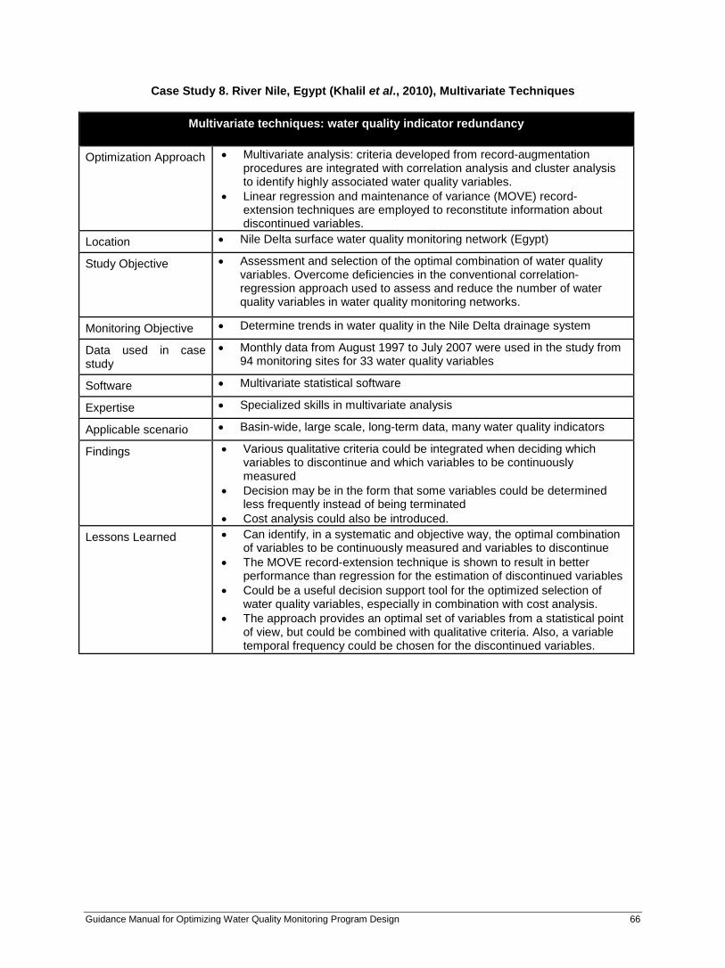
Case Study 8. River Nile, Egypt (Khalil et al., 2010), Multivariate Techniques

Multivariate techniques: water quality indicator redundancy Optimization Approach • Multivariate analysis: criteria developed from record-augmentation

procedures are integrated with correlation analysis and cluster analysis to identify highly associated water quality variables.

• Linear regression and maintenance of variance (MOVE) record-extension techniques are employed to reconstitute information about discontinued variables.

Location • Nile Delta surface water quality monitoring network (Egypt)

Study Objective • Assessment and selection of the optimal combination of water quality variables. Overcome deficiencies in the conventional correlation-regression approach used to assess and reduce the number of water quality variables in water quality monitoring networks.

Monitoring Objective • Determine trends in water quality in the Nile Delta drainage system


• Monthly data from August 1997 to July 2007 were used in the study from 94 monitoring sites for 33 water quality variables

Software • Multivariate statistical software

Expertise • Specialized skills in multivariate analysis

Applicable scenario • Basin-wide, large scale, long-term data, many water quality indicators

Findings • Various qualitative criteria could be integrated when deciding which variables to discontinue and which variables to be continuously measured

• Decision may be in the form that some variables could be determined less frequently instead of being terminated

• Cost analysis could also be introduced. Lessons Learned • Can identify, in a systematic and objective way, the optimal combination

of variables to be continuously measured and variables to discontinue • The MOVE record-extension technique is shown to result in better

performance than regression for the estimation of discontinued variables • Could be a useful decision support tool for the optimized selection of

water quality variables, especially in combination with cost analysis. • The approach provides an optimal set of variables from a statistical point

of view, but could be combined with qualitative criteria. Also, a variable temporal frequency could be chosen for the discontinued variables.


Case Study 9. Mississippi River, Louisiana (Ozkul et al., 2000), Entropy Analysis

Entropy analysis: spatial coverage and temporal frequency

Optimization tool

• Entropy Analysis • The approach permits the selection of a particular space/time alternative

design feature for a specified level of redundant information to be retained in the network. The method evaluates the redundancy of information between successive observations.

Location • Mississippi River Louisiana, basin 07

Study Objective • Optimize network

Monitoring Objective • Long-term trend in water quality using physico-chemical variables (DO, EC, Cl-, TSS, P, COD, NO3, -N)


• 12 sampling stations (Louisiana Department of Environmental Quality, Office of Water Resources); 27 years (between 1966 and 1992); monthly measurements of 26 water quality variables;

• Over 3 years of monitoring data Software • Relatively sophisticated statistical (including multivariate analysis) and

analytical software; database/data management software Expertise • High: statistical and analytical skills, knowledge of entropy equation and

analysis Applicable Scenario • Large scale, river basin, long-term

Findings • Monthly sampling was extended to bimonthly frequency for some variables for other variables further decreases were indicated

• Existing monthly sampling can be increased to bimonthly sampling intervals. For some variables further increases are indicated.

Lessons Learned • Provides a quantitative measure of the information content of a sampling site and of an observed time series

• Gives an indication of data utility • Can be used to assess jointly several features of a network (e.g.,,

sampling sites, sampling frequencies, variables to be sampled, and sampling duration)

• Gives alternative designs for sampling sites and respective sampling intervals, that can be compared to cost

• Sensitive to the selection of the appropriate multivariate probability density function to represent the multivariate nature of a network. The authors recommend to use different techniques in combination and to investigate network features from different perspectives


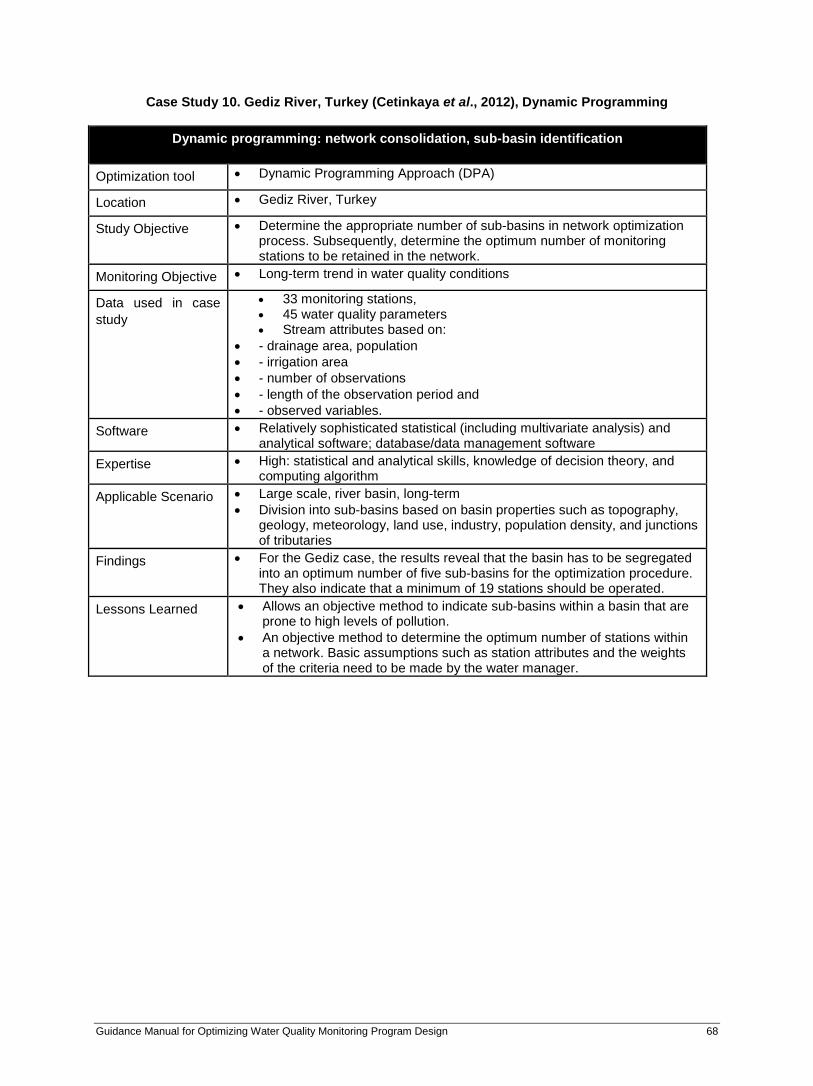
Case Study 10. Gediz River, Turkey (Cetinkaya et al., 2012), Dynamic Programming

Dynamic programming: network consolidation, sub-basin identification Optimization tool • Dynamic Programming Approach (DPA)

Location • Gediz River, Turkey

Study Objective • Determine the appropriate number of sub-basins in network optimization process. Subsequently, determine the optimum number of monitoring stations to be retained in the network.

Monitoring Objective • Long-term trend in water quality conditions


• 33 monitoring stations, • 45 water quality parameters • Stream attributes based on:

• - drainage area, population • - irrigation area • - number of observations • - length of the observation period and • - observed variables.

Software • Relatively sophisticated statistical (including multivariate analysis) and analytical software; database/data management software

Expertise • High: statistical and analytical skills, knowledge of decision theory, and computing algorithm

Applicable Scenario • Large scale, river basin, long-term • Division into sub-basins based on basin properties such as topography,

geology, meteorology, land use, industry, population density, and junctions of tributaries

Findings • For the Gediz case, the results reveal that the basin has to be segregated into an optimum number of five sub-basins for the optimization procedure. They also indicate that a minimum of 19 stations should be operated.

Lessons Learned • Allows an objective method to indicate sub-basins within a basin that are prone to high levels of pollution.

• An objective method to determine the optimum number of stations within a network. Basic assumptions such as station attributes and the weights of the criteria need to be made by the water manager.


Case Study 11. Ijsselmeer Netherlands (Schulze and Bouma 2001), Artificial Neural Network

Artificial Neural Network (ANN): spatial optimization

Optimization Approach • Artificial Neural Network, linear modeling, multivariate transfer models

Location • Ijsselmeer, Netherlands • Ijsselmeer was chosen because of its complex character for water flow

direction, changing wind directions and water depth Study Objective • Determine if ANN contributes to spatial optimization of the Ijsselmeer

water quality network. • Linear modelling (ARX Modelling) was used to find relationships between

locations. • Models between locations were multivariate transfer models. • Chloride was used as the pilot parameter to find out the use of ANN for

prediction of the time series; chloride was chosen because of the quality of the time series (no gaps).

Monitoring Objective • Determine the trend in water quality


• Time series (1992-1998, 12 or 24 measurements per year) of parameters were chosen from different parameter groups (chloride, nitrate, phosphorus, lead, TSS)

• Criteria for parameter selection: presence at high concentrations, representative for soluble parameters and particular parameters

• Criteria for locations: water flow direction, location of issue, present and future function of the water system, and subjects and policy aims.

Software • Statistical software package • NEURAL-Computing • Once calibrated or trained, the ANN can be easily transformed into a

program code so anyone can use it Expertise Strong statistical and computational skills

Requirements for the construction of a neural network are: • Representative data • Software and hardware with enough memory and capacity • Close cooperation with respect to the discipline concerned • Knowledge of construction of an ANN and statistics to validate the

models • Good tool, if enough representative data is available, but knowledge of

individual processes are meager Applicable Scenario • Lakes, dynamic process, long–term, large scale

Findings • ANN can be used for developing complex monitoring networks for detection of trends and casualties.

Lessons Learned • ANN is a multi-use modelling tool to describe all types of relations between cause and effect

• Every relation between cause and effect can be modelled • No assumptions need to be made considering the nature of the

relationship • Preprocessing of data is minimal • The problem is presented as a black box instead of studying the process

itself • With respect to the degree of freedom there is a risk of over-

parameterization • It is not possible to simulate scenarios with other boundary conditions

since the ANN did not learn how to handle these situations.


Case Study 12. River Nile, Egypt (Khalil et al., 2011), Artificial Neural Network

Artificial Neural Network: spatial coverage

Optimization Approach • PCA was used to select water quality variables that best explain water quality variability in the Nile delta drainage. The first step was to divide the Nile Delta into sub-units. The second step involved identification of attributes for each of the 94 sub-units.

• Attributes used: cultivated area (ha); average soil salinity (ppm); average soil hydraulic conductivity (m per day); average total annual rainfall (mm per year); drainage system total length (km); average total industrial effluent (m3 per day); waste water treatment plants total capacity (m3 per day); number of livestock; and average annual applied fertilizers (tons per year)

• Maintenance Of Variance Extension (MOVE) was used to extend the records of the discontinued variables

• Regression incorporates water quality data with basin attributes to identify the optimal combination of locations to be discontinued, locations to be continuously measured and sub-basins where locations should be added.

Location • River Nile, Egypt

Study Objective • Determine if the current sampling locations are representative of the different categories of sub-catchments within the Nile Delta

• Divide the monitored basin into clusters of spatial units with similar attributes and apply a stratified optimum sampling strategy to spatially distribute the monitoring locations for the establishment of a new water quality monitoring network

• MOVE3 and ANN techniques are applied to reconstitute information about variables at discontinued locations using the data from the case study.

Monitoring Objective • Determine general water quality


• Stream flow and 27 water quality variables at 50 locations

Software • Hybrid-cluster algorithm, ANN

Expertise • Specialized statistical and computational skills, ANN expertise

Applicable Scenario • Large scale dataset with many water quality variables

Findings • 11 groups of similar subunits were identified • 4 groups are over-monitored, and four are under-monitored • 11 stations can be discontinued.

Lessons Learned • The approach can systematically and objectively assess and identify the monitoring locations to be continuously measured, the locations to be discontinued and the locations to be added

• It allows for the reconstitution of information about water quality variables at discontinued locations

• Introduction of a cost analysis would help to address the trade-off between the number of water quality monitoring locations and the temporal frequency.


References for Appendix A

Beveridge D., St-Hilaire A., Ouarda TB, Khalil B., Conly F.M., Wassenaar L.I., & E. Ritson-Bennett (2012): A

geostatistical approach to optimize water quality monitoring networks in large lakes. Application to Lake Winnipeg. In Journal of Great Lakes Research 38, pp. 174–182.

Cetinkaya C.P. & N.B. Harmancioǧlu (2012): Assessment of Water Quality Sampling Sites by a Dynamic Programming Approach. In Journal of Hydrologic Engineering 17, pp. 305–317.

Dowdall M., Gerland S., Karcher M, Gwynn J.P., Rudjord A.L., & Kolstad A.K (2005): Optimisation of sampling for the temporal monitoring of technetium-99 in the Arctic marine environment. In Journal of Environmental Radioactivity 84, pp. 111-130

Harmancioǧlu N., Fistikoglu O., Ozkul S.D., Singh V.P. & M.N. Alpaslan (1999): Water quality monitoring network design. Water Science and Technology. Dordrecht/Boston/London: Kluwer Academic Publisher (33), 290 pp.

Hunt C.D., Field J., Rust S. & P. Burke. (2006): Surface Water Quality Monitoring Network Optimization. Comprehensive Report to the South Florida Water Management District. 87 pp. http://www.sfwmd.gov/portal/page/portal/xrepository/sfwmd_repository_pdf/comp_optimza_rpt.pdf

Hunt C.D., Steven W. Rust & L. Sinnott (2008): Application of statistical modeling to optimize a coastal water quality monitoring program. In Environmental Monitoring and Assessment 137, pp. 505-522.

Khalil B., Ouarda T.B., M.J St-Hilaire A. Chebana F. (2010): A statistical approach for the rationalization of water quality indicators in surface water quality monitoring networks. In Journal of Hydrology 386 (1-4), pp. 173–185.

Khalil, B.; Ouarda T. B., & M. J. St-Hilaire (2011): A statistical approach for the assessment and redesign of the Nile Delta drainage system water-quality-monitoring locations. In Journal of Environmental Monitoring 13 (8), p. 2910.

Ozkul S., Harmancioǧlu N.B. & V.P. Singh. (2000): Entropy-Based Assessment of Water Quality Monitoring Networks. In Journal of Hydrologic Engineering 5 (1), pp. 90–100.

Schulze F.H. & F.H. Bouma. (2001): Use of artificial neural networks in integrated water management. Proceedings Monitoring Tailor-made III - 333-342.

Strobl, R.O., Robillard P.D., Shannon R.D., Day R.L. & A.J. McDonnell (2006 a): A Water Quality Monitoring Network Design Methodology for the Selection of Critical Sampling Points: Part I. In Environmental Monitoring and Assessment 112: 137 – 158.

Redfield, G., Rawlik, P. & L. Lindstrom (2008): Strategies for Reengineering Water Quality Monitoring in Florida. South Florida Environmental Report. 44 pages. http://www.sfwmd.gov/portal/page/portal/pg_grp_sfwmd_sfer/portlet_sfer/tab2236041/volume1/chapters/v1_ch_1b.pdf

Strobl, R.O., Robillard P.D., Shannon R.D., Day R.L. & A.J. McDonnell (2006b): A water quality monitoring network design methodology for the selection of critical sampling points: Part II. In Environ Monit Assess 122 (1-3), pp. 319–334.

Swertz, O.C, Laane R.W.P & K.J.M. Kramer (1997): An assessment of water quality monitoring in the Dutch coastal zone: Needs, Aims and Optimization. Monitoring Tailor-made I.


http://www.sfwmd.gov/portal/page/portal/xrepository/sfwmd_repository_pdf/comp_optimza_rpt.pdf

Appendix B - Tables


Table B- 1. Common Monitoring Goals for Rivers (Hydromorphological, Physico-Chemical and Biological Variables) (adapted from European Communities, 2003)

Common Monitoring Variables used in River Monitoring with respective Monitoring Goals

Hum

an H

ealth

Use

Clim

ate

Cha

nge

Ant

hrop

ogen

ic A

ctiv

ities

an

d M

odifi

catio

ns

Aci

dific

atio

n

Eutr

ophi

catio

n

Org

anic

Con

tam

inat

ion

Sedi

men

tatio

n

Toxi

c C

onta

min

atio

n

Agr

icul

tura

l, D

omes

tic o

r In

dust

rial D

isch

arge

Wat

er U

se/R

egul

atio

n

Floo

d C

ontr

ol

Fish

erie

s

Exot

ic S

peci

es

Hab

itat A

vaila

bilit

y

Rivers: Hydromorphological Variables

Quantity and Dynamic of Flow x x x

River Continuity x x

River Depth and Width Variation x x

Structure and Substrate of the River Bed

x x

Structure of the Riparian Zone x x

Rivers: Physico-Chemical Variables

Thermal Condition (Temperature)

x X

Oxygenation (Dissolved Oxygen, Biological Oxygen Demand)

x x X

Salinity (Potassium, Magnesium, Sodium, Chloride, Sulfates, Carbonates)

x X

Organic Matter, Total Suspended Solids

x x x x

Acidification (pH, Alkalinity) x X

Nutrients (Ammonia, Nitrite, Nitrate, Total Phosphorus, Soluble Reactive Phosphorus)

x x x x X

Metals (various), Persistent Organic Pollutants (Pesticides, PCBs)

x x x X

Rivers: Biological Variables

Bacteria (E.coli) x

Benthic Invertebrates x x x

Macrophytes x x


Table B-2. Common Monitoring Goals for Lakes (Hydromorphological, Physico-Chemical and Biological Variables) (adapted from European Communities, 2003)

Lakes: Common Monitoring Variables with Respective

Monitoring Goals

Hum

an H

ealth

Use

Clim

ate

Cha

nge

Ant

hrop

ogen

ic A

ctiv

ities

an

d M

odifi

catio

ns

Aci

dific

atio

n

Eutr

ophi

catio

n

Org

anic

Con

tam

inat

ion

Sedi

men

tatio

n

Toxi

c C

onta

min

atio

n

Agr

icul

tura

l, D

omes

tic o

r In

dust

rial D

isch

arge

Wat

er U

se/R

egul

atio

n

Floo

d co

ntro

l

Hyd

ro-m

orph

olog

ical

al

tera

tion

Fish

erie

s

Exot

ic s

peci

es

Hab

itat A

vaila

bilit

y

Lakes: Hydromorphological Variables

Quantity and dynamic of flow x x x x x x x

Residence time (volume, depth, inflow, outflow)

x x x x x x x x

Lake depth variation (surface, volume, depth)

x x x x x x

Quantity, structure and substrate of lake bed

x x x x x x x x x

Structure of lake shore (length, riparian vegetation cover, species present, bank

x x x x x x x x

Lakes: Physico-Chemical Variables Transparency (Secchi, Turbidity)

x x

Thermal Condition (Temperature)

x

Oxygenation (Dissolved Oxygen, Biological Oxygen Demand, Organic Matter)

x x x x

Salinity (Potassium, Magnesium, Sodium, Chloride, Sulfates,

x x

Acidification (pH) x x x Nutrients (Ammonia, Nitrite, Nitrate, Total Phosphorus, Soluble Reactive Phosphorus, Chlorophyll a)

x x x c


x x x

Lakes: Biological Variables Phytoplankton x x x x x x

Macrophytes x x x x x x x

Phytobenthos x x x x x x x

Benthic invertebrates x x x x x x x

Fish x x x x x x x


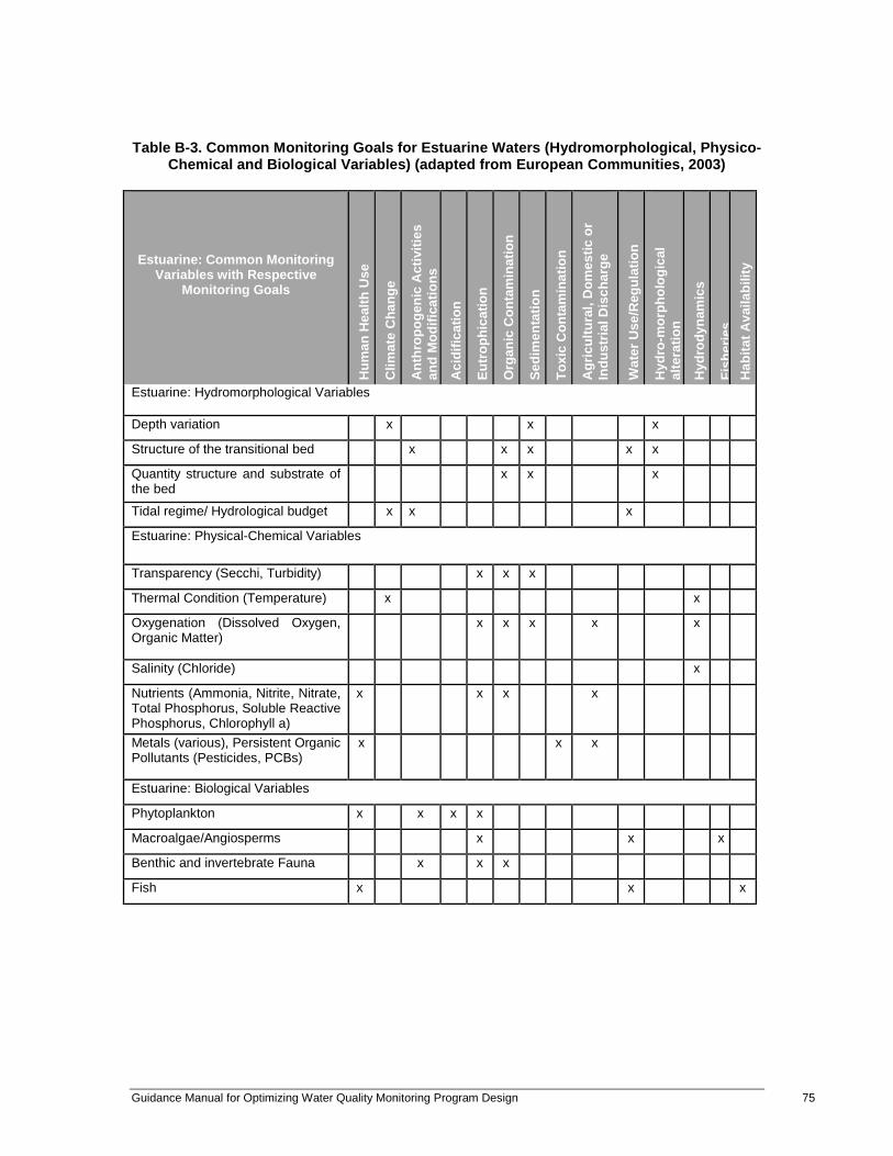
Table B-3. Common Monitoring Goals for Estuarine Waters (Hydromorphological, Physico-Chemical and Biological Variables) (adapted from European Communities, 2003)

Estuarine: Common Monitoring Variables with Respective

Monitoring Goals

Hum

an H

ealth

Use

Clim

ate

Cha

nge

Ant

hrop

ogen

ic A

ctiv

ities

an

d M

odifi

catio

ns

Aci

dific

atio

n

Eutr

ophi

catio

n

Org

anic

Con

tam

inat

ion

Sedi

men

tatio

n

Toxi

c C

onta

min

atio

n

Agr

icul

tura

l, D

omes

tic o

r In

dust

rial D

isch

arge

Wat

er U

se/R

egul

atio

n

Hyd

ro-m

orph

olog

ical

al

tera

tion

Hyd

rody

nam

ics

Fish

erie

s H

abita

t Ava

ilabi

lity

Estuarine: Hydromorphological Variables

Depth variation x x x

Structure of the transitional bed x x x x x

Quantity structure and substrate of the bed

x x x

Tidal regime/ Hydrological budget x x x

Estuarine: Physical-Chemical Variables

Transparency (Secchi, Turbidity) x x x

Thermal Condition (Temperature) x x

Oxygenation (Dissolved Oxygen, Organic Matter)

x x x x x

Salinity (Chloride) x

Nutrients (Ammonia, Nitrite, Nitrate, Total Phosphorus, Soluble Reactive Phosphorus, Chlorophyll a)

x x x x


x x x

Estuarine: Biological Variables Phytoplankton x x x x

Macroalgae/Angiosperms x x x

Benthic and invertebrate Fauna x x x

Fish x x x


Table B-4. Common Monitoring Goals for Coastal Waters (Hydromorphological, Physico-Chemical and Biological Variables) (adapted from European Communities, 2003)

Coastal: Common Monitoring Variables with Respective Monitoring Goals

Hum

an H

ealth

Use

Clim

ate

Cha

nge

Ant

hrop

ogen

ic A

ctiv

ities

an

d M

odifi

catio

ns

Eutr

ophi

catio

n

Org

anic

Con

tam

inat

ion

Sedi

men

tatio

n

Toxi

c C

onta

min

atio

n

Hyd

rody

nam

ics

Fish

erie

s

Coastal: Hydromorphological Variables

Depth variation

Structure and substrate of the coastal bed structure

x x

Structure of the intertidal zone x

Direction of dominant currents x x

Wave exposure x

Coastal: Physico-Chemical Variables

Transparency (Secchi, Turbidity) x x x

Thermal Condition (Temperature) x x

Oxygenation (Dissolved Oxygen, Organic Matter)

x

Salinity (Chloride) x x

Nutrients (Ammonia, Nitrite, Nitrate, Total Phosphorus, Soluble Reactive Phosphorus, Chlorophyll a)

x x x x


x x

Coastal: Biological Variables

Phytoplankton x x x

Macroalgae x x x x

Benthic and invertebrate Fauna x x x x

Fish x


Table B- 5. Recommended Annual Frequency for Rivers, Lakes, Estuarine and Coastal Water Bodies (adapted from European Communities, 2003, Gems, 2005)

Type

of M

onito

ring

Type of Water Quality Variables

Temporal Frequency

Riv

ers

Lake

s

Tran

sitio

nal

Coa

stal

Bas

elin

e M

onito

ring medium - high very high

minimum: 4 (including high and low water

stage optimum: 24 (i.e. fortnightly

sampling, and weekly)

Minimum: 1 at turnover

optimum: 1 vertical profile at

end of stratification

period

N/A

N/A

Surv

eilla

nce

Thermal Conditions

3/year 3/year 3/year 3/year

Oxygenation 3/year 3/year 3/year 3/year

Salinity 3/year 3/year 3/year 3/year

Nutrient Status 3/year 3/year 3/year 3/year

Acidification 3/year 3/year 3/year 3/year

Phytoplankton 2/year 2 per year 2/year 2/ year

Other aquaticflora 3 years 3 years 3 years 3 years

Macro invertebrates

3 years 3 years 3 years 3 years

Fish 3 years 3 years 3 years 3 years

Continuity 6 years N/A N/A N/A

Hydrology continuous 12/year N/A N/A

Morphology 6 years 6 years 6 years 6 years


Table B- 6. Type of Monitoring in Relation to Key Monitoring Design Aspects (Number of Monitoring Variables, Temporal and Spatial Frequency). Level of Effort is Indicated for the

Design Aspects. (adapted from Chapman et al., 1996)

Type of monitoring

Number of water quality variables

Temporal frequency

Duration Lag

Multi-objective

Medium medium 12 per year

medium > 5 years

medium 1 year

Common Water Quality Monitoring

Baseline Monitoring

medium – high very high

once per year - 4 years

Operational surveillance

Specific medium variable short (month, week)

Trend monitoring

low for single objective high for multiple objectives

very high > 10 years > 1 year

Specific Water Quality Monitoring

Background Monitoring

low -high low variable medium

Preliminary survey

High low to medium (depending on objective)

short < 1 year short (month)

Emergency surveys

contaminant inventory

high very short (days- weeks)

very short (days- weeks)

Impact Survey

Specific medium variable short-to medium

Modelling Survey

specific variables specific (diel cycles)

short to medium two periods (calibration, vaildation)

short

Early warning surveys

very limited continuous unlimited instantaneous


guidance manual for optimizing water qualtiy monitoring

Documents