guide to the demonstration of equivalence of ambient...
TRANSCRIPT
GUIDE TO THE DEMONSTRATION OF EQUIVALENCE
OF AMBIENT AIR MONITORING METHODS
Report by an EC Working Group on Guidance for the Demonstration of Equivalence

Guidance to Demonstration of Equivalence January 2010
2
TABLE OF CONTENTS
1 INTRODUCTION..................................................................................................................5
2 REFERENCES TO STANDARDS ............................ ............................................................6
3 TERMS, DEFINITIONS AND ABBREVIATIONS ............... ...................................................7
3.1 TERMS AND DEFINITIONS................................................................................................................. 7 3.2 ABBREVIATIONS.............................................................................................................................. 7
4 DEFINITION OF EQUIVALENCE.......................... ...............................................................8
5 PROCEDURE FOR DEMONSTRATION OF EQUIVALENCE ......... ...................................10
5.1 FLOW SCHEME............................................................................................................................... 10 5.2 GENERAL....................................................................................................................................... 10 5.3 SCOPE OF EQUIVALENCE CLAIMS................................................................................................... 12
5.3.1 Limiting conditions ............................................................................................................... 12 5.3.2 Generalization of equivalence claims and mutual use of measurement results.................... 12 5.3.3 Extent of tests required ......................................................................................................... 13
5.4 PRACTICAL APPROACH TO EQUIVALENCE TESTING........................................................................ 15 5.5 REQUIREMENTS FOR LABORATORIES............................................................................................. 16 5.6 OPERATION OF THE EQUIVALENT METHOD.................................................................................... 17
6 SELECTING A TEST PROGRAMME......................... ........................................................17
6.1 GENERAL....................................................................................................................................... 17 6.2 MEASUREMENT METHODOLOGY.................................................................................................... 18 6.3 MEASUREMENT TRACEABILITY ..................................................................................................... 18 6.4 SPECIFICATION OF TEST PROGRAMMES.......................................................................................... 18
7 TEST PROGRAMME 1 - MANUAL METHODS FOR GASES AND VAP OURS..................20
7.1 GENERAL....................................................................................................................................... 20 7.2 OVERVIEW OF THE TEST PROCEDURES........................................................................................... 20 7.3 LABORATORY TEST PROGRAMME.................................................................................................. 21
7.3.1 Test programme 1A: pumped sampling ................................................................................ 21 7.3.2 Test Programme 1B. Diffusive sampling .............................................................................. 29
7.4 FIELD TEST PROGRAMME............................................................................................................... 30 7.4.1 General ................................................................................................................................. 30 7.4.2 Experimental conditions ....................................................................................................... 31 7.4.3 Evaluation of the field test data ............................................................................................ 32 7.4.4 Evaluation of results of field tests......................................................................................... 34
8 TEST PROGRAMME 2 - AUTOMATED MEASUREMENT SYSTEMS FO R GASES..........35
8.1 GENERAL....................................................................................................................................... 35 8.2 OVERVIEW OF THE TEST PROCEDURES........................................................................................... 35 8.3 DEFINITIONS APPLICABLE TO AUTOMATED MEASUREMENT SYSTEMS............................................ 37 8.4 LABORATORY TESTS...................................................................................................................... 37
8.4.1 Test concentrations............................................................................................................... 37 8.4.2 Response time ....................................................................................................................... 37 8.4.3 Short–term drift .................................................................................................................... 38 8.4.4 Repeatability for continuous measuring CMs....................................................................... 39 8.4.5 Carry over and repeatability for CMs collecting samples onto a sorbent prior to analysis. 40 8.4.6 Lack of fit (linearity)............................................................................................................. 40 8.4.7 Difference between sample and calibration port.................................................................. 41 8.4.8 Effect of short-term fluctuations in concentration (averaging test)...................................... 42 8.4.9 Variation in sample-gas pressure......................................................................................... 43 8.4.10 Variation in sample-gas temperature ................................................................................... 44

Guidance to Demonstration of Equivalence January 2010
3
8.4.11 Surrounding temperature variation ...................................................................................... 44 8.4.12 Variation due to supply voltage............................................................................................ 45 8.4.13 Cross-sensitivity to interfering substances ........................................................................... 46 8.4.14 NO2 converter efficiency....................................................................................................... 49
8.5 FIELD TEST.................................................................................................................................... 50 8.5.1 General ................................................................................................................................. 50 8.5.2 Experimental conditions ....................................................................................................... 50 8.5.3 Evaluation of data collected ................................................................................................. 50
8.6 DETERMINATION OF THE COMBINED MEASUREMENT UNCERTAINTY ............................................. 53 8.7 CALCULATION OF THE EXPANDED LABORATORY UNCERTAINTY OF CANDIDATE METHOD............. 54 8.8 EVALUATION OF TEST RESULTS..................................................................................................... 54
9 TEST PROGRAMME 3 – METHODS FOR PARTICULATE MATTER.. ..............................55
9.1 GENERAL....................................................................................................................................... 55 9.2 OVERVIEW OF THE TEST PROCEDURE............................................................................................. 55 9.3 LABORATORY TEST PROGRAMME.................................................................................................. 56
9.3.1 General ................................................................................................................................. 56 9.3.2 Application of automated filter changers ............................................................................. 56 9.3.3 Different weighing conditions............................................................................................... 57
9.4 FIELD TEST PROGRAMME............................................................................................................... 57 9.4.1 General ................................................................................................................................. 57 9.4.2 Experimental conditions ....................................................................................................... 58 9.4.3 Requirements for quality control .......................................................................................... 59
9.5 EVALUATION OF DATA COLLECTED ............................................................................................... 59 9.5.1 General ................................................................................................................................. 59 9.5.2 Suitability of datasets............................................................................................................ 59 9.5.3 Calculation of performance characteristics ......................................................................... 59 9.5.5 Calculation of the expanded uncertainty of candidate method............................................. 63
9.6 EVALUATION OF RESULTS OF FIELD TESTS..................................................................................... 63 9.7 APPLICATION OF CALIBRATION FUNCTIONS................................................................................... 63 9.8 EXAMPLES..................................................................................................................................... 65 9.9 ONGOING QA/QC, MAINTENANCE AND VERIFICATION OF THE EQUIVALENT METHOD.................. 65
9.9.1 Ongoing QA/QC and maintenance....................................................................................... 65 9.9.2 Ongoing verification of equivalence..................................................................................... 65
10 TEST PROGRAMME 4 – SPECIATED PARTICULATE MATTER .... ..............................67
10.1 GENERAL....................................................................................................................................... 67 10.2 OVERVIEW OF THE TEST PROCEDURES........................................................................................... 67 10.3 LABORATORY TEST PROGRAMME.................................................................................................. 67
10.3.1 General ................................................................................................................................. 67 10.3.2 Test programme.................................................................................................................... 68
10.4 FIELD TEST PROGRAMME............................................................................................................... 72 10.4.1 General ................................................................................................................................. 72 10.4.2 Experimental conditions ....................................................................................................... 73 10.4.3 Evaluation of test results ...................................................................................................... 73 10.4.4 Evaluation of results of field tests......................................................................................... 75
11 REPORTING REQUIREMENTS .....................................................................................76
12 REFERENCES ...............................................................................................................77
ANNEX A............................................ ......................................................................................79
ANNEX B............................................ ......................................................................................80
ANNEX C..................................................................................................................................82

Guidance to Demonstration of Equivalence January 2010
4
ANNEX D..................................................................................................................................83
ANNEX E..................................................................................................................................86
ANNEX F ..................................................................................................................................87

Guidance to Demonstration of Equivalence January 2010
5
1 INTRODUCTION One of the objectives of the European legislation on ambient air quality is to ‘assess the ambient air quality in Member States on the basis of common methods and criteria’. Currently, two Directives are in force: � Directive 2008/50/EC on ambient air quality and cleaner air for Europe [1] � Directive 2004/107/EC relating to arsenic, cadmium, mercury, nickel and polycyclic aromatic
hydrocarbons in ambient air [2]. These Directives give limit or target values for specific atmospheric pollutants, and by referring to EN standards developed by CEN Technical Committee (TC) 264 “Air Quality” specify the reference methods to be used for the measurement of concentrations of these pollutants. In addition, they specify data quality objectives (DQO) that have to be met for the performance of specific measurement tasks. These data quality objectives include minimum requirements for: � expanded uncertainties of measurement results in the region of the limit or target value(s) set
for each pollutant � time coverage of the measurements in relation to the reference period of the limit or target
values � data capture when using the measurement method, i.e., effective measurement time. CEN TC 264’s remit when developing the standards was to ensure these were validated against the data quality objectives given in the relevant Directives. In order to harmonize the approaches of the various ambient air working groups, in particular for the assessment of the measurement uncertainties, a CEN Report was prepared in which the principles for these uncertainty assessments are laid down (report CR 14377). A Member State (MS) when implementing the directives should use the reference methods, but the Directives allow a member state to ‘use any other method which it can demonstrate gives results equivalent to the above (reference) method’.
Figure 1. Building blocks for equivalence demonstration This report describes the principles and methodologies to be used for the demonstration of the equivalence of methods other than the EU reference methods. It is intended for use by laboratories nominated by National Competent Authorities (see Directive 2008/50/EC) to perform the tests relevant to the demonstration of equivalence of ambient-air measurement methods. The building blocks of the equivalence demonstration procedure are presented in Figure 1.
Demonstration of Equivalence
1. Definition of Equivalence
2. General procedure
3. Scope of equivalence
claims
4. Requirements for test
laboratories
5. Test and evaluation
programmes
6. Reporting requirements
7. Ongoin g QA/QC
(+verification)

Guidance to Demonstration of Equivalence January 2010
6
2 REFERENCES TO STANDARDS This clause incorporates by dated or undated reference, provisions from other publications. These normative references are cited at the appropriate places in the text and the publications are listed hereafter. For dated references, subsequent amendments to or revisions of any of these publications apply to this only when incorporated in it by amendment or revision. For undated references the latest edition of the publication referred to applies. EN 12341 1998 Air Quality – Determination of the PM10 fraction of suspended
particulate matter – Reference method and field test procedure to demonstrate reference equivalence of measurements
ENV 13005 1999 Guide to the expression of uncertainty in measurement EN 14907 2005 Ambient Air Quality – Reference gravimetric measurement
method for the determination of the PM2.5 mass fraction of suspended particulate matter in ambient air.
EN-ISO 17025 2005 General requirements for the competence of testing and
calibration laboratories CR 14377 2001 Approach to uncertainty estimation for ambient-air
measurement methods EN-ISO 14956 2001 Air quality – Evaluation of the suitability of a measurement
method by comparison with a stated measurement uncertainty EN 13528 pt1 2002 Ambient air quality – Diffusive samplers for the determination of
gases and vapours – Requirements and test methods – Part 1: General requirements
EN13528 pt2 2002 Ambient air quality – Diffusive samplers for the determination of
gases and vapours – Requirements and test methods – Part 2: Specific requirements and test methods.
EN13528 pt3 2003 Ambient air quality – Diffusive samplers for the determination of
gases and vapours – Part 3: Guide to selection, use and maintenance.
ISO 6142 2000 Gas analysis. Preparation of calibration gas mixtures –
Gravimetric methods ISO 6143 2000 Gas analysis. Comparison methods for the determination of
calibration gas mixtures ISO 6144 2002 Gas analysis. Preparation of calibration gas mixtures – Static
volumetric methods ISO 6145 Gas analysis. Preparation of calibration gas mixtures – Dynamic
volumetric methods. All Parts

Guidance to Demonstration of Equivalence January 2010
7
3 TERMS, DEFINITIONS AND ABBREVIATIONS 3.1 Terms and definitions 3.1.1 Automated
(Measurement) Method/System
A measurement method or system performing measurements or samplings of a specified pollutant in an automated way
3.1.2 Candidate method A measurement method proposed as an alternative to the relevant reference method for which equivalence has to be demonstrated
3.1.3 Equivalent method A measurement method other than the reference method for the measurement of a specified air pollutant for which equivalence has been demonstrated
3.1.4 Fixed measurements Measurements taken at fixed sites, either continuously or by random sampling, to determine the levels in accordance with the relevant data quality objectives. [1 Art. 2]
3.1.5 Limit value A level fixed on the basis of scientific knowledge, with the aim of avoiding, preventing or reducing harmful effects on human health and/or the environment as a whole, to be attained within a given period and not to be exceeded once attained. [1]
3.1.6 Manual (measurement) method
A measurement method by which sampling is performed on site, with sample analysis performed in the laboratory.
3.1.7 National Competent Authority
Authority or body designated by a Member State as responsible for the approval of measurement systems (methods, equipment, networks and laboratories). [1 Art. 3]
3.1.8 Reference method EN standard method referred to in Directive 2008/50/EC Annex VI and Directive 2004/107/EC as the reference method for the measurement of a specified ambient air pollutant.
3.1.9 Target value A level fixed with the aim of avoiding more long-term harmful effects on human health and/or the environment as a whole, to be attained where possible over a given period. [1]
3.2 Abbreviations AMS Automated Measurement System
CM Candidate Method
CRM Certified Reference Material DQO Data Quality Objective
EC European Commission
EU European Union
IR Infrared
MM Manual Method MS Member State
NCA National Competent Authority
PM Particulate Matter
PSM Primary Standard Material
PT Proficiency Testing RM Reference Method
UV Ultraviolet

Guidance to Demonstration of Equivalence January 2010
8
4 DEFINITION OF EQUIVALENCE Within the framework of air quality measurements, the definition of equivalence is laid down in a document specifying ‘Terms of Reference for CEN/TC 264 Ambient-air Standards’ (see e.g. Report CR 14377 Annex C). These Terms of Reference state that methods other than the reference method may be used for the implementation of the directives provided that they fulfil the minimum data quality objectives specified in the relevant directive. Therefore, considering the intended use of the reference methods, the following definition will be used for the demonstration of equivalence:
‘An equivalent method to the reference method for the measurement of a specified air pollutant, is a method meeting the data quality objectives for fixed measurements specified in the relevant air quality directive’
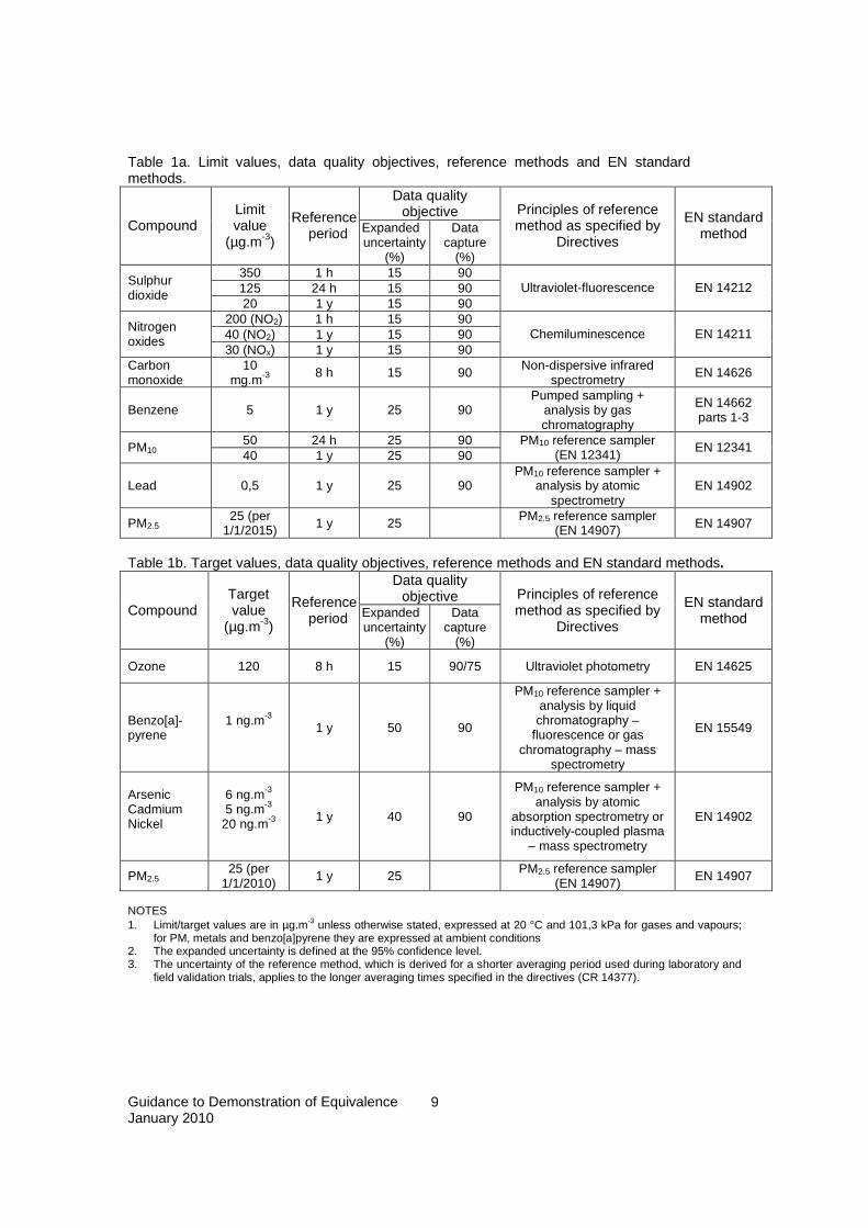
Data quality objectives set in [1] and [2] are for data capture, time coverage and measurement uncertainty, the latter to be assessed in the region of the limit or target value set for the specified pollutant (see 1). In conformance with the requirements of [1] and [2] the measurement uncertainty for comparison with the uncertainty data quality objective shall be evaluated in accordance with GUM, implying that all known biases in the results of the equivalent method shall be eliminated. NOTE 1. The use of the reference methods is not restricted to fixed measurements. NOTE 2. Where a candidate method fails to meet the uncertainty data quality objective of the reference method, it may still be able to meet the uncertainty data quality objective for indicative methods. However, it is not an “equivalent method” in the strict sense of this Guide. NOTE 3. For automated measurement systems for gases all relevant uncertainty sources must be assessed and the Candidate method must pass all the prescribed individual performance criteria, in addition to the overall uncertainty criteria, in order to conform with all the requirements of the relevant EN standards. NOTE 4. Equivalence may be granted for regional situations within a Member State, but also for situations encompassing more than one Member State. The latter case offers an incentive for Member States’ cooperation in the performance of equivalence testing. Tables 1a and 1b give an overview of limit or target values, data quality objectives, reference methods and reference methods for pollutants under Directives 2008/50/EC and 2004/107/EC which are within the scope of this document. Limit values and target values are relevant as they set requirements for the demonstration of equivalence (see above).
Guidance to Demonstration of Equivalence January 2010
9
Table 1a. Limit values, data quality objectives, reference methods and EN standard methods.
Data quality objective
Compound Limit value
(µg.m-3)
Reference period Expanded
uncertainty (%)
Data capture
(%)
Principles of reference method as specified by
Directives
EN standard method
350 1 h 15 90 125 24 h 15 90
Sulphur dioxide
20 1 y 15 90 Ultraviolet-fluorescence EN 14212
200 (NO2) 1 h 15 90 40 (NO2) 1 y 15 90
Nitrogen oxides
30 (NOx) 1 y 15 90 Chemiluminescence EN 14211
Carbon monoxide
10 mg.m-3 8 h 15 90 Non-dispersive infrared
spectrometry EN 14626
Benzene 5 1 y 25 90 Pumped sampling +
analysis by gas chromatography
EN 14662 parts 1-3
50 24 h 25 90 PM10 40 1 y 25 90 PM10 reference sampler
(EN 12341) EN 12341
Lead 0,5 1 y 25 90 PM10 reference sampler +
analysis by atomic spectrometry
EN 14902
PM2.5 25 (per
1/1/2015) 1 y 25 PM2.5 reference sampler (EN 14907) EN 14907
Table 1b. Target values, data quality objectives, reference methods and EN standard methods.
Data quality objective
Compound Target value
(µg.m-3)
Reference period Expanded
uncertainty (%)
Data capture
(%)
Principles of reference method as specified by
Directives
EN standard method
Ozone 120 8 h 15 90/75 Ultraviolet photometry EN 14625
Benzo[a]-pyrene
1 ng.m-3 1 y 50 90
PM10 reference sampler + analysis by liquid chromatography –
fluorescence or gas chromatography – mass
spectrometry
EN 15549
Arsenic Cadmium Nickel
6 ng.m-3 5 ng.m-3
20 ng.m-3 1 y 40 90
PM10 reference sampler + analysis by atomic
absorption spectrometry or inductively-coupled plasma
– mass spectrometry
EN 14902
PM2.5 25 (per
1/1/2010) 1 y 25 PM2.5 reference sampler (EN 14907) EN 14907
NOTES 1. Limit/target values are in µg.m-3 unless otherwise stated, expressed at 20 °C and 101,3 kPa for gases and vapours;
for PM, metals and benzo[a]pyrene they are expressed at ambient conditions 2. The expanded uncertainty is defined at the 95% confidence level. 3. The uncertainty of the reference method, which is derived for a shorter averaging period used during laboratory and
field validation trials, applies to the longer averaging times specified in the directives (CR 14377).

Guidance to Demonstration of Equivalence January 2010
10
5 PROCEDURE FOR DEMONSTRATION OF EQUIVALENCE 5.1 Flow scheme A flow scheme depicting the procedure for equivalence demonstration is given in Figure 2. 5.2 General A Member State may propose methods that deviate from the reference method defined in the ambient air quality directives [1-2] and elaborated in the EN standard methods [3-13] given in Table 1. Consequently, the responsibility for the demonstration of equivalence of the proposed candidate method rests with the National Competent Authority (NCA). This authority bears responsibility for the quality of national air quality monitoring data. In the process of demonstrating equivalence (see Figure 2) the NCA may delegate its responsibility to a National Reference Laboratory. However, the NCA remains responsible for the final decision on the acceptance or rejection of a candidate method as equivalent to the reference method, and for reporting to the European Commission.
The initiative for the use of ‘equivalent’ methods may arise from an NCA or from a national or regional laboratory performing air quality measurements related to the implementation of the ambient air quality directives. In the latter case, the laboratory proposing the use of a method shall notify its NCA, and perform a preliminary assessment of the candidate method in order to ensure that the method:
� fulfils the requirements of data capture and time coverage set for the continuous/fixed measurements; e.g., a candidate method for the measurement of concentrations of nitrogen dioxide for comparison with the 1-hour limit value, shall be able to provide a data capture of 90% or more for hourly averaged measurement results, and
� has the potential for meeting the uncertainty data quality objective at the limit or target value
concentration for continuous or fixed measurements of the specified pollutant. In this preliminary assessment results from external studies may be considered subject to fulfilling the conditions given in 5.3.2.2.
When the candidate method passes this preliminary assessment, the test and evaluation programme relevant to the candidate method can be selected using the flow scheme given in Figure 2.
If at any stage of the test programme the measurement uncertainty of the candidate method fails to meet the relevant Directive’s uncertainty criterion, then the equivalence evaluation may be terminated, and a report of the results obtained prepared for the NCA. This may be used as a basis to reduce relevant uncertainty sources - after which tests appropriate to these uncertainty sources may be repeated, and the resulting uncertainty again compared with the uncertainty criterion.
Following completion of the relevant test and evaluation programme, the results of these tests and evaluations shall be reported to the NCA. The NCA will then decide on the acceptance or rejection of the candidate method as an equivalent method. In the case of acceptance, an evaluation report with conclusions should be submitted to the European Commission for review. The European Commission in its review may wish to consult a committee of experts about the claim for equivalence.
The NCA shall ensure that each individual measurement performed in the Member State for the purpose of assessment of air quality under the Directives fulfils provisions of the Directives. This implies that a procedure must be in place for evaluation as to whether the implementation of the equivalent method at each measurement site is appropriate, i.e., whether the equivalence claim can be generalized to that site if it was not included in the original equivalence demonstration.

Guidance to Demonstration of Equivalence January 2010
11
Guidance to Demonstration of Equivalence January 2010
12
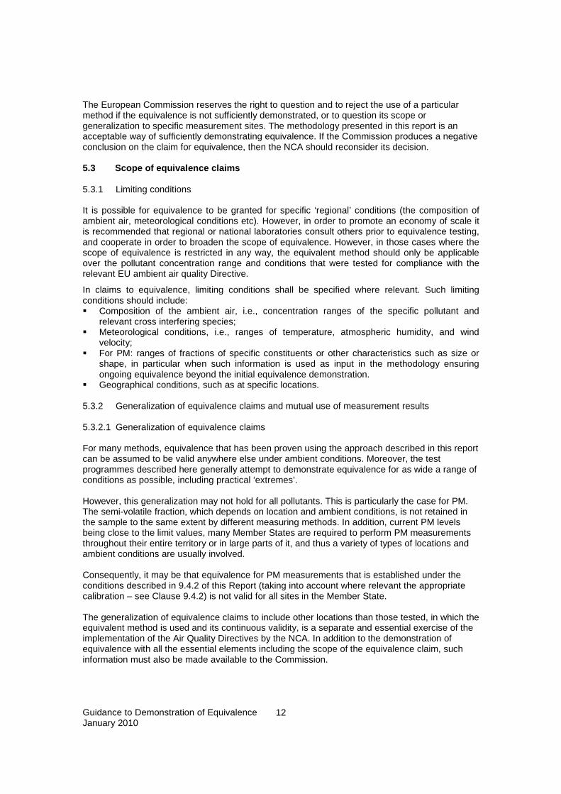
The European Commission reserves the right to question and to reject the use of a particular method if the equivalence is not sufficiently demonstrated, or to question its scope or generalization to specific measurement sites. The methodology presented in this report is an acceptable way of sufficiently demonstrating equivalence. If the Commission produces a negative conclusion on the claim for equivalence, then the NCA should reconsider its decision. 5.3 Scope of equivalence claims 5.3.1 Limiting conditions It is possible for equivalence to be granted for specific ‘regional’ conditions (the composition of ambient air, meteorological conditions etc). However, in order to promote an economy of scale it is recommended that regional or national laboratories consult others prior to equivalence testing, and cooperate in order to broaden the scope of equivalence. However, in those cases where the scope of equivalence is restricted in any way, the equivalent method should only be applicable over the pollutant concentration range and conditions that were tested for compliance with the relevant EU ambient air quality Directive.
In claims to equivalence, limiting conditions shall be specified where relevant. Such limiting conditions should include: � Composition of the ambient air, i.e., concentration ranges of the specific pollutant and
relevant cross interfering species; � Meteorological conditions, i.e., ranges of temperature, atmospheric humidity, and wind
velocity; � For PM: ranges of fractions of specific constituents or other characteristics such as size or
shape, in particular when such information is used as input in the methodology ensuring ongoing equivalence beyond the initial equivalence demonstration.
� Geographical conditions, such as at specific locations. 5.3.2 Generalization of equivalence claims and mutual use of measurement results 5.3.2.1 Generalization of equivalence claims For many methods, equivalence that has been proven using the approach described in this report can be assumed to be valid anywhere else under ambient conditions. Moreover, the test programmes described here generally attempt to demonstrate equivalence for as wide a range of conditions as possible, including practical ‘extremes’. However, this generalization may not hold for all pollutants. This is particularly the case for PM. The semi-volatile fraction, which depends on location and ambient conditions, is not retained in the sample to the same extent by different measuring methods. In addition, current PM levels being close to the limit values, many Member States are required to perform PM measurements throughout their entire territory or in large parts of it, and thus a variety of types of locations and ambient conditions are usually involved. Consequently, it may be that equivalence for PM measurements that is established under the conditions described in 9.4.2 of this Report (taking into account where relevant the appropriate calibration – see Clause 9.4.2) is not valid for all sites in the Member State. The generalization of equivalence claims to include other locations than those tested, in which the equivalent method is used and its continuous validity, is a separate and essential exercise of the implementation of the Air Quality Directives by the NCA. In addition to the demonstration of equivalence with all the essential elements including the scope of the equivalence claim, such information must also be made available to the Commission.

Guidance to Demonstration of Equivalence January 2010
13
Developing a detailed procedure for generalization of equivalence claims is beyond the scope of this Guide. There is no objective procedure for delineating the monitoring sites where a demonstrated equivalence is valid and where it is not. Instead, expert judgment, based on the similarities in conditions that prevail at the various relevant locations, is needed for this. There are several relevant ways of describing the sites where a demonstrated equivalence is valid. The sites may be classified in similar groups of locations using station types (that are characterized primarily by the nearby sources). The validity range of a demonstrated equivalence can also be described by listing the regions (parts of the Member State) of validity. A combination of station types and regions (e.g. rural stations in regions A, B and C) may also be a useful way. From this description, a list of stations with the calibrations applied can be derived and tabled in the report to the Commission. 5.3.2.2 Mutual use of test results The considerations given above should also apply to the use of results of studies in other networks or Member States. Additionally, before using such data, it should be ascertained that: � The candidate method is applied in the same configuration in which it has been tested, using
the same calibration function; the potential effects of data acquisition and processing procedures shall be taken into consideration.
� The candidate method is applied under a rigorous regime of ongoing QA/QC in each of those networks or Member States.
� The results of the original PM equivalence tests remain valid within each network or Member States by ongoing verification of equivalence (see 5.6 and 9.9).
In addition, it is strongly recommended that those networks or Member States sharing results shall periodically compare results of verification tests and shall periodically perform side-by-side comparisons using the candidate method. Because of these constraints it may be favourable for networks or Member States to cooperate within equivalence test programmes a priori. 5.3.3 Extent of tests required Within this report, the extent of equivalence testing is specified on the basis of the differences between the reference method and the candidate method. These differences can – in principle – be separated into two groups (defined subsequently in this report as ‘variations on a theme’ and ‘different methodologies’). 5.3.1.1 Variations on a theme Minor parts of the reference method can be modified resulting in ‘variations on a theme’. Examples of ‘possible variations’ are: � The use of different converters to transform nitrogen dioxide into nitric oxide in
chemiluminescence analysers; � The use of different scrubbers for ozone; � The use of different sampling media/substrates, e.g., sorbents and filter types; � The use of different procedures for analyte recovery, e.g., for recovery of benzene from
sorbent tubes, and metals and polycyclic aromatic hydrocarbons (PAH) from PM samples;

Guidance to Demonstration of Equivalence January 2010
14
� The use of different analytical procedures, e.g., modifications to the chromatographic separation for benzene and PAH analysis, and to the atomic spectrometric conditions for metals analysis;
� The use of different PM filter storage procedures; � The use of automated filter changers for manual PM samplers. 5.3.3.2 Different methodologies A candidate method may be based on a different measurement principle. Possible examples of different principles are: � Automated measurement systems for benzene using ultraviolet spectrometry as the detection
technique; � Sampling of particulate matter using a sampling inlet with characteristics differing from those
specified in PM10 and PM2.5 standards for the reference sampler; � Measurement of particulate matter using automated methods, e.g., based on β-ray
attenuation or on oscillating microbalances; � Use of in-situ optical measurement techniques for particulate matter; � Use of different analytical techniques for the measurement of relevant compounds in sample
extracts, e.g., liquid chromatography for benzene, inductively-coupled plasma – optical emission spectrometry for metals;
� Measurement of gases and vapours using diffusive sampling instead of pumped sampling or
automated methods; � Automated measurement of gases based on a different spectrometric technique, e.g., fourier-
transform infrared spectrometry (FTIR) for sulphur dioxide; � Measurement of gases using pumped sampling instead of automated methods. 5.3.3.3 Practical implications In practice, the possible use of different methodologies is limited. Based on practical potential/current applications, the following may be considered as relevant examples of the underlying principles (a complete method includes complete specifications of sampling media, calibration procedures and their frequencies, etc: Sulphur dioxide, nitrogen dioxide, carbon monoxide, ozone The reference method is continuous spectrometry. Candidate methods of practical value include: � Diffusive sampling with subsequent sample analysis12
1 Diffusive sampling is particularly suited for producing results for compliance testing with long-term – e.g., annual – limit or target values. 2 A number of studies exist – although not performed as prescribed in this report – indicating that diffusive sampling methods for nitrogen dioxide may fulfil the uncertainty data quality objective for, at minimum, indicative measurements [see, e.g., 16, 17].
Guidance to Demonstration of Equivalence January 2010
15
� Continuous spectrometric techniques using measurement principles other than those described by the standard methods.
Benzene The reference method is pumped sampling (automated or non-automated) followed by sample analysis using gas chromatography. Candidate methods of practical value are: � Diffusive sampling with subsequent sample analysis � Continuous spectrometry � Automated measurement using ultraviolet spectrometry after sample enrichment. EN standard methods exist for the measurement of benzene by diffusive sampling and analysis by gas chromatography after thermal or solvent desorption of benzene samples (EN 14662 parts 4 and 5; refs. 14,15).3 Particulate matter The reference method is manual pumped sampling onto a filter substrate using a pre-specified aerosol classifier followed by gravimetric analysis. Candidate methods may be: � Semi-continuous automated methods based on mass measurement, such as ß-ray
attenuation or (tapered-element) oscillating microbalance � Continuous methods based on optical techniques. Metals, benzo[a]pyrene The reference method is based on sampling of the PM10 aerosol fraction of the total suspended particulate matter in ambient air, with subsequent analysis using atomic absorption spectrometry or inductively-coupled plasma mass spectrometry (metals), or gas or liquid chromatography (benzo[a]pyrene). The candidate methods may be based on: � Use of alternative analytical techniques; � Use of alternative aerosol samplers (see under particulate matter). 5.4 Practical approach to equivalence testing In principle, the approach to equivalence testing described in this report comprises four phases, i.e.: � An initial non experimental pre-assessment to check whether the candidate method has the
potential for fulfilling the data quality objectives in the directives on data capture and measurement uncertainty
� Assessment of the uncertainty of the candidate method using an approach based on the
principles of ENV 13005 (clause 8) in a series of laboratory tests
3 The validation studies performed within the frame of the drafting of these standards – although not performed as prescribed in this report – indicate that these methods may fulfil the uncertainty data quality objective for fixed measurements.

Guidance to Demonstration of Equivalence January 2010
16
� The performance of a series of field tests for confirmation of the findings of the laboratory tests in which the candidate method is tested side-by-side to the reference method; the ‘lack-of-comparability’ is tested on the basis of the performance of linear regression with symmetric treatment of both variables, i.e., with uncertainties attributed to both variables
� The evaluation of the resulting uncertainties by comparison of
� laboratory uncertainty and the uncertainty data quality objective � field uncertainty and laboratory uncertainty � field uncertainty and the uncertainty data quality objective.
This approach has the advantage that – in the case of ‘variations on a theme’ – only those contributions to uncertainty that arise from the variation need to be assessed. For example, if a new extraction agent is used, the uncertainty contributions to be tested are the extraction efficiency, blank levels and analytical selectivity. This implies a priori knowledge of the uncertainty contributions of all relevant uncertainty sources in the standard method. In addition, for manual candidate methods for which only the analytical principle but not the sample preparation component differs from the standard method (e.g., the use of ICP-OES for the analysis of metals) only the contributions relevant to the use of the different analytical method need to be quantified. An exception to this is made for the reference methods using automated measurement systems for gases; for these, all relevant uncertainty sources must be assessed in order to avoid the use of the equivalence procedure as an route for monitors that have failed the test criteria of the EN standards for automated measurement systems for these species being accepted as equivalent. In general, for particulate matter the test programmes are restricted to field tests only [3]. It should be noted that measurement procedures based on separate sampling and analysis may be open to ‘variations’ in parts of the procedure that can lead to systematic differences in measurement results produced by different laboratories on ‘identical’ air samples. This has been shown to introduce a significant additional contribution to measurement uncertainty – that due to inter-laboratory variability. Consequently, where necessary, the test procedure shall involve more than one laboratory in order to evaluate the contributions to uncertainty from ‘between-laboratory’ variations. Finally, it should be noted that application of the approach described in this report is not mandatory. Other approaches that are in conformity with the requirements of ENV 13005 can also be used, provided that the user can prove the validity of the alternative approach. 5.5 Requirements for laboratories The laboratories performing the required tests shall be independent of manufacturers or suppliers of equipment used for implementing the candidate method.
Both reference and candidate methods shall be operated under appropriate regimes of quality assurance/quality control (QA/QC). Consequently, the laboratories performing the tests necessary for the demonstration of equivalence shall be able to demonstrate technical competence for these tests. These may be the laboratory/laboratories already using the candidate and/or reference method, but may also be different laboratories, subject to fulfilment of the requirements for laboratories. It is strongly recommended that laboratories work in full compliance with the requirements of EN-ISO 17025, as demonstrated through a formal accreditation for the application of the reference as well as the candidate method.
In the absence of a formal accreditation, compliance with the requirements of EN-ISO 17025 should be demonstrated through an independent audit performed by an auditor with specific experience in the use of the relevant reference and candidate methods. A demonstration of competence by achieving acceptable performance in a suitable Proficiency Testing (PT) scheme

Guidance to Demonstration of Equivalence January 2010
17
is considered useful additional information. In the absence of such a scheme, measurements of a series of appropriate test samples with satisfactory results are strongly recommended for demonstrating competence. Test samples shall be such that the concentration(s) of the compound(s) to be measured is (are) traceable to primary standard materials (PSM) or certified reference materials (CRM).
NOTE For the purpose of the supply of suitable test samples, the National Competent Authority may consult an appropriate National Reference Laboratory and/or accreditation body. 5.6 Operation of the equivalent method Equivalence tests are performed within a limited timeframe. In order to ensure that claims to equivalence remain valid, the practical operation of the equivalent method shall be subject to an appropriate regime of ongoing quality assurance/quality control (QA/QC). This regime shall be documented in the Standard Operating Procedure describing the operation of the method. Minimum requirements for ongoing QA/QC shall be as reliable as the requirements given in appropriate EN standard methods for automated or manual methods [3-13]. In addition, it is recommended that field tests are performed periodically, by operating reference and equivalent methods in parallel, in order to check whether the claim to equivalence of the measurement results remains valid. For PM such tests are mandatory, and are elaborated in 9.9. 6 SELECTING A TEST PROGRAMME 6.1 General Figure 3 gives a flow scheme for selection of the appropriate test programme for any candidate method. Four different test programmes have been elaborated for four distinct situations. The distinctions are based in principle on whether: 1. There are ‘stated references’ that exist for the establishment of measurement traceability, or
the extent to which it is possible to quantify all contributions to measurement uncertainty from comparisons starting from primary measurement standards ( ENV 13005).
2. The measurement methodology is automated or manual, i.e., based on separate sampling and analysis.
The consequences of these distinctions are explained below.
Figure 3. Flow scheme for selection of test programme
Does CM involve speciation of PM ?
Does CM involve sampling of PM ?
Is CM based on AMS ?
Test Programme 4 Speciated Particulate Matter
Test Programme 3 Non-speciated Particulate Matter
Test Programme 2 Automated Measurement Systems for
gases and vapours
YES
Test Programme 1 Manual Method for gases and
vapours
NO
NO
YES
NO
YES
Guidance to Demonstration of Equivalence January 2010
18
6.2 Measurement methodology
Test procedures will differ for automated and manual methods for the measurement of gases; for automated methods the method will be tested more or less as a ‘black box’ (e.g., [4]); for manual methods separate steps in the measurement procedure will be subject to uncertainty evaluation in the laboratory tests (e.g., [8]). 6.3 Measurement traceability The structure and contents of the test programmes given here are determined by the extent to which measurement results can be made traceable to SI units. The existence of primary measurement standards or certified reference materials enables laboratory tests to be performed in which these standards and materials can be used to evaluate measurement bias. For gaseous and vaporous compounds measurement results can be made fully traceable to SI units through existing primary measurement standards prepared in accordance with ISO 6142, ISO 6144 or ISO 6145. This situation applies to continuous measurements of sulphur dioxide, nitrogen oxides, carbon monoxide and benzene. For ozone, UV photometry is defined, by convention, as an ‘absolute’ measurement methodology. A UV photometer of which the measurement uncertainty has been evaluated from first principles may be termed a ‘reference’ photometer. For measurements of benzene using pumped sampling methods, reference materials and standards exist through which both the results of the sampling and the analysis can be made fully traceable to SI units. For heavy metals and benzo[a]pyrene reference materials are available which provide traceability for the analytical component of the measurement procedure. However, these generally have sample matrices and measurand concentrations that differ considerably from those relevant to the implementation of the EU Directives. For example, available reference materials for speciated PM measurements – such as NIST SRM 1648 and 1649a – differ in matrix (bulk sample instead of filter), particle size (up to 125 µm) and composition from the reference materials that would be required. Representative reference materials currently do not exist. For the measurement of particulate matter a more complicated situation exists as no relevant metrological standards or reference materials exist for establishing the traceability of PM10 and PM2.5 measurements to SI units. Results of measurements of sample volume and sampled mass of particulate matter can be made traceable to SI, but there is no suitable primary standard available to assess the contribution of other uncertainty components of the measurement method. The uncertainty of any candidate method therefore has to be determined with reference to a PM reference sampler as specified in EN 12341 for PM10, assuming these ‘reference samplers’ to be unbiased with respect to the applied particle-size convention. 6.4 Specification of test programmes Test Programme 1 refers to manual methods for gases and vapours (benzene, carbon monoxide, sulphur dioxide, nitrogen dioxide and ozone). � Test Programme 1A: Laboratory test programme for variations on the reference method;
laboratory and field test programme for pumped sampling alternatives to reference methods for other gaseous pollutants
� Test Programme 1B: Laboratory and field test programmes for diffusive sampling analogous
to test programmes of EN 13528.

Guidance to Demonstration of Equivalence January 2010
19
Test Programme 2 refers to alternative automated measurement systems for gases and vapours, (benzene, carbon monoxide, sulphur dioxide, nitrogen dioxide and ozone) e.g., using other spectrometric techniques. Test Programme 3 refers to alternative methodologies for the monitoring of non-speciated particulate matter. Test programme 3 includes testing of a size selective inlet, when this differs from that of the PM reference sampler. Test Programme 4 refers to the determination of speciated particulate matter (metals and benz[a]pyrene in samples of particulates).

Guidance to Demonstration of Equivalence January 2010
20
7 TEST PROGRAMME 1 - MANUAL METHODS FOR GASES AND V APOURS 7.1 General This test programme describes a procedure for determining whether a candidate method (CM) is suitable to be considered equivalent to the reference methods for the measurement of gases and vapours in ambient air [4-10], using manual measurement methods (with separate sampling and analysis). This test programme is suitable for evaluating: � pumped and diffusive sampling methods as alternatives for automated methods for the
measurement of sulphur dioxide, nitrogen dioxide, carbon monoxide, ozone and benzene � diffusive sampling methods and modified pumped sampling methods as alternatives for
benzene. 7.2 Overview of the test procedures Testing for equivalence will normally be carried out in two parts: a laboratory test in which the contributions of the different uncertainty sources to the measurement uncertainty will be assessed, and a field test in which the candidate method will be tested side-by-side with the relevant standard method. If a CM is a modification to an existing EN standard method, then only the laboratory performance characteristics that are affected by the modification need to be tested and their standard uncertainties calculated. The standard uncertainties associated with the affected performance characteristics shall then be used together with these existing standard uncertainties for the other characteristics, to determine again the combined measurement uncertainty. If a CM utilises a measurement methodology that is different to a standard method, then all of the tests shall be performed. In both cases the results of existing studies, when demonstrably obtained according to the requirements of this test procedure, may be used to determine standard uncertainties. The CM should be tested in a way that is representative of its practical use; for example, the frequencies of tests (e.g., response drift) and re-calibrations (e.g., flow rates) that are used in practice should be applied in the test programmes. For diffusive sampling methods for benzene, information on uncertainty sources exists in EN standards [14,15]; these standards should be consulted when alternative diffusive sampling methods are considered as candidate methods. For diffusive sampling of inorganic gases, no such information is currently available in this form. It is necessary to compile and evaluate this information in the course of the validation of diffusive sampling methods for these gases. Test programme 1 consists of a laboratory and field test programme. The laboratory test programme is separated into two parts (1A and 1B), covering methods for which the volume of air sampled can be made traceable to SI units (pumped sampling) and to methods for which this is not possible (diffusive sampling). Candidate methods must pass the criteria for the laboratory test programme, and also pass the criteria for the field test programme. Only candidate methods that pass the laboratory test programme shall proceed to the field test programme.

Guidance to Demonstration of Equivalence January 2010
21
7.3 Laboratory test programme In the laboratory test programme, the uncertainty sources listed in Table 2 are considered and assessed, where appropriate. Table 2. Laboratory test programme 1: uncertainty sources
Symbol Uncertainty source Pumped
sampling Diffusive sampling
1 Sample volume Vsam 1.2 Sample flow / uptake rate 1.2.1 calibration and measurement 1.2.2 variation during sampling
ϕ υ
1.3 Sampling time t t 1.4 Conversion to standard temperature and pressure 2 Mass of compound in sample msam msam 2.1 Sampling efficiency E * 2.2 Compound stability A A 2.3 Extraction/desorption efficiency D D 2.4 Mass of compound in calibration standards mCS mCS 2.5 Response factors 2.5.1 lack-of-fit of calibration function 2.5.2 analytical repeatability 2.5.3 drift between calibrations
F d
F d
2.6 Selectivity R R 3 Mass of compound in blank mbl mbl
* For diffusive sampling, sampling efficiency is incorporated in the uptake rate. The uncertainty sources that require assessment depend on the differences between candidate and standard methods as follows: Is the candidate method based on a different measurement principle? In that case, the full test programme needs to be performed. Does the sampling principle of the candidate method differ from that of the reference method (e.g. diffusive instead of pumped sampling for benzene)? In this case, uncertainty source 1.2 needs to be assessed. Does the analytical principle of the candidate method differ from that of the reference method, with the sampling being the same? In this case, the uncertainty sources under 2.5, 2.6 and 3 need to be assessed. Is the candidate method a modification of the reference method? In this case, the uncertainty sources relevant to the modification need to be investigated, e.g. � 2.1, 2.2, 2.3 and 3 for alternative sorbents � 2.3 and 2.6 for alternative extraction solvents � 2.5 and 2.6 for alternative analytical configurations. 7.3.1 Test programme 1A: pumped sampling 7.3.1.1 Sampled volume of air The sampled volume of air shall be sufficient to allow reliable quantification of the pollutant concentration at the lower end of the measurement range (10% of the limit value). In practice, the sampled volume of air may be determined in two ways:
Guidance to Demonstration of Equivalence January 2010
22
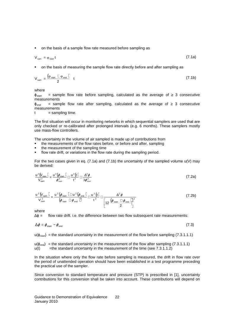
� on the basis of a sample flow rate measured before sampling as
tV startsam φ= (7.1a)
� on the basis of measuring the sample flow rate directly before and after sampling as
( )t
2V endstart
sam
φφ += (7.1b)
where ϕstart = sample flow rate before sampling, calculated as the average of ≥ 3 consecutive measurements ϕend = sample flow rate after sampling, calculated as the average of ≥ 3 consecutive measurements t = sampling time. The first situation will occur in monitoring networks in which sequential samplers are used that are only checked or re-calibrated after prolonged intervals (e.g. 6 months). These samplers mostly use mass-flow controllers. The uncertainty in the volume of air sampled is made up of contributions from � the measurements of the flow rates before, or before and after, sampling � the measurement of the sampling time � flow rate drift, or variations in the flow rate during the sampling period. For the two cases given in eq. (7.1a) and (7.1b) the uncertainty of the sampled volume u(V) may be derived:
( ) ( ) ( )2
2
2
2
2
2
2
2
startstart 3ϕϕ
ϕϕ ∆++=
ttuu
VVu start
sam
sam (7.2a)
( ) ( ) ( )( )
( )( ) 2
2
2
2
2
22
2
2
212
+
∆+++
+=
endstartendstart
endstart
sam
sam
t
tuuu
V
Vu
ϕϕϕ
ϕϕϕϕ (7.2b)
where ∆ϕ = flow rate drift. i.e. the difference between two flow subsequent rate measurements:
endstart ϕϕϕ −=∆ (7.3) u(ϕstart) = the standard uncertainty in the measurement of the flow before sampling (7.3.1.1.1) u(ϕend) = the standard uncertainty in the measurement of the flow after sampling (7.3.1.1.1) u(t) =the standard uncertainty in the measurement of the time (see 7.3.1.1.2) In the situation where only the flow rate before sampling is measured, the drift in flow rate over the period of unattended operation should have been established in a test programme preceding the practical use of the sampler. Since conversion to standard temperature and pressure (STP) is prescribed in [1], uncertainty contributions for this conversion shall be taken into account. These contributions will depend on

Guidance to Demonstration of Equivalence January 2010
23
whether mass-flow controlled or volume-controlled sampling devices are used. The calculation of individual uncertainty contributions is given in 7.3.1.1.3. 7.3.1.1.1 Sample flow calibration and measurement The uncertainty in the measurement of the flow rates before and after sampling is calculated from the uncertainty in the readings of the flow meter used which can be derived from calibration certificates, assuming the calibration is fully traceable to primary standards of flow, and the uncertainty of the actual flow rate measurement results, as
( )2
22
2
2
ϕϕϕ n
suu
meascal +
= (7.4)
where u(ϕ) = the standard uncertainty in the measurement of flow ucal = uncertainty due to calibration of the flow meter smeas = standard deviation of individual flow measurements, determined from ≥ 3 measurements n = number of flow measurements performed under practical conditions of use. 7.3.1.1.2 Sampling time The sampling time t should be measured to within ± 0,5 min. Then for a sampling time of 8 hours or more the relative uncertainty due to the measurement of t is negligible. 7.3.1.1.3 Conversion of sample volume to STP Mass-flow controlled sampling devices For mass-controlled sampling devices a conversion of the sample volume to STP may be affected by direct conversion of measured flow rates to values at STP. For conversion, the following equation is used:
( )273293
3,101 +=
TP
STP ϕϕ (7.6)
where ϕSTP = sample flow converted to STP ϕ = actual measured sample flow P = actual air pressure during the flow measurements (in kPa) T = actual air temperature during the flow measurements (in °C). By modification of Eq. (7.1) through substitution of φ with φSTP , the sample volume converted to STP is:
tV STPstartSTPsam ,, ϕ= (7.7a)
( )
tV STPendSTPstartSTPsam ⋅
+=
2,,
,
ϕϕ (7.7b)
The uncertainty contribution for mass-flow controlled sampling devices can then be obtained by extending equation (7.4) to:
Guidance to Demonstration of Equivalence January 2010
24
( ) ( ) ( )2
2
2
2
2
22
2
2
TTu
PPun
suu
meascal
STP
STP +++
=ϕϕ
ϕ (7.8)
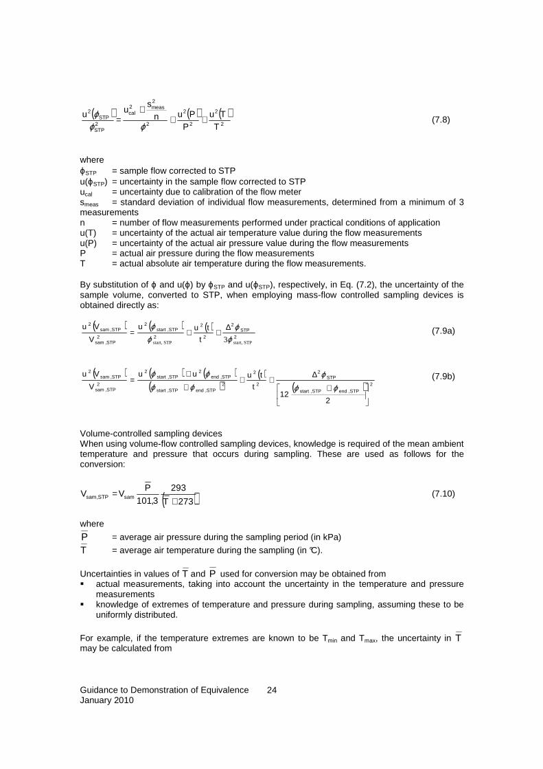
where ϕSTP = sample flow corrected to STP u(ϕSTP) = uncertainty in the sample flow corrected to STP ucal = uncertainty due to calibration of the flow meter smeas = standard deviation of individual flow measurements, determined from a minimum of 3 measurements n = number of flow measurements performed under practical conditions of application u(T) = uncertainty of the actual air temperature value during the flow measurements u(P) = uncertainty of the actual air pressure value during the flow measurements P = actual air pressure during the flow measurements T = actual absolute air temperature during the flow measurements. By substitution of ϕ and u(ϕ) by ϕSTP and u(ϕSTP), respectively, in Eq. (7.2), the uncertainty of the sample volume, converted to STP, when employing mass-flow controlled sampling devices is obtained directly as:
( ) ( ) ( )2
2
2
2
2
,2
2,
,2
STPstart,STPstart, 3ϕϕ
ϕϕ STPSTPstart
STPsam
STPsam
t
tuu
V
Vu ∆++= (7.9a)
( ) ( ) ( )( )
( )( ) 2
,,
2
2
2
2,,
,2
,2
2,
,2
212
+
∆++
+
+=
STPendSTPstart
STP
STPendSTPstart
STPendSTPstart
STPsam
STPsam
t
tuuu
V
Vu
ϕϕ
ϕϕϕ
ϕϕ (7.9b)
Volume-controlled sampling devices When using volume-flow controlled sampling devices, knowledge is required of the mean ambient temperature and pressure that occurs during sampling. These are used as follows for the conversion:
( )273T
2933,101
PVV samSTP,sam +
= (7.10)
where
P = average air pressure during the sampling period (in kPa)
T = average air temperature during the sampling (in °C).
Uncertainties in values of T and P used for conversion may be obtained from � actual measurements, taking into account the uncertainty in the temperature and pressure
measurements � knowledge of extremes of temperature and pressure during sampling, assuming these to be
uniformly distributed.
For example, if the temperature extremes are known to be Tmin and Tmax, the uncertainty in T may be calculated from

Guidance to Demonstration of Equivalence January 2010
25
( )12
TTu)T(u
2minmax2
cal2 −+= (7.11)
where ucal = uncertainty due to calibration of the temperature meter. Generally, the first term will be negligible compared to the second. The above uncertainty contributions are then combined to give the uncertainty in the sample volume converted to STP for volume-controlled sampling devices as:
( ) ( ) ( ) ( )2
2
2
2
2sam
sam2
2STP,sam
STP,sam2
P
Pu
T
TuVVu
V
Vu++= (7.12)
7.3.1.2 Mass of compound sampled The mass of a compound sampled may be expressed as:
DAEm
m meassam ⋅⋅
= (7.13)
where E = sampling efficiency A = compound stability in the sample D = extraction/desorption efficiency mmeas = measured mass of compound in the analytical sample (extract, desorbate) before correction. A correction for extraction/desorption efficiency shall be applied when D is significantly different from 1 (see 7.3.2.1.3). 7.3.1.2.1 Sampling efficiency For the sampling medium to be used the breakthrough volume shall be determined under reasonable worst-case conditions. In practice, these conditions will consist of a combination of a high concentration, high temperature, high air humidity, and the presence of high levels of potentially interfering compounds. As the worst-case conditions will vary between sample locations, test conditions may be adapted to these local conditions. The sample volume shall be less than half the experimentally established breakthrough volume. In that case the sampling efficiency will be 100% and will not contribute to the uncertainty in msam. 7.3.1.2.2 Compound stability The compound stability shall be established experimentally through storage under conditions (time, temperature, environment) that are typical to the individual monitoring network. Tests shall be performed at a compound level corresponding to the ambient air limit or target value. At times t=0 and t=t, n samples shall each be analyzed under repeatability conditions (n ≥ 6). For both times the samples shall be randomly selected from a batch of representative samples in order to minimize possible systematic concentration differences. As a test of (in)stability, a t-test will be performed (95% confidence, 2-sided). The t-test must show no significant difference

Guidance to Demonstration of Equivalence January 2010
26
between results obtained at the start and end of the stability test. The uncertainty of the stability determination consists of contributions from: � extraction/desorption (random part of extraction/desorption efficiency) � calibration (random part of calibration) � analytical precision � inhomogeneity of the sample batch. However, the uncertainty contribution of the determination of stability will already be covered by contributions determined in Clause 7.3.1.2.3 and it therefore does not need to be taken into account separately. 7.3.1.2.3 Extraction/desorption efficiency The extraction/desorption efficiency of the compound from the sample and its uncertainty are typically obtained from replicate measurements on certified reference materials (CRMs). The uncertainty due to incomplete extraction/desorption for the level corresponding to the limit value is calculated from contributions of � the uncertainty in the concentration of the CRM � the standard deviation of the mean mass determined as
( )
2CRM
D2
CRM2
2
2
mn
ms)m(u
D
)D(u += (7.14)
where mCRM = certified mass in the CRM s(mD) = standard deviation of the replicate measurement results of the mass determined n = number of replicate measurements of the CRM. When D is significantly different from 1 (at the 95% confidence level), the measurement result shall be corrected (see eq. (7.1)). The value of s(mD) is used as an indicator of the relative uncertainty due to analytical repeatability wanal:
( )2D
D2
2anal m
msw = (7.15)
7.3.1.2.4 Corrections to the measured mass of the compound The uncertainty in the measured mass of a compound is determined by � the uncertainty in the concentrations of the calibration standards used � the lack-of-fit of the calibration function � drift of detector response between calibrations � the precision of the analysis � the selectivity of the analytical system used. Calibration standards The uncertainty of the concentration of a compound in the calibration standards used will depend on the type of calibration standard used. For a tube standard prepared by sampling from a standard atmosphere it will depend on:

Guidance to Demonstration of Equivalence January 2010
27
� the uncertainty of the concentration in the generated standard atmosphere; uncertainty assessments for this parameter can be found in ISO 6144 and 6145 [18,19]
� the uncertainty of the sampled volume of the standard atmosphere. The uncertainty is calculated as
( )2
2
2sa
sa2
2cs
cs2
VVu
C)C(u
m)m(u += (7.16)
where u(mcs) = uncertainty in the mass in the calibration standard (mcs) u(Csa) = uncertainty in the concentration in the standard atmosphere (Csa) u(V) = uncertainty in the volume of the standard atmosphere sampled (V). For calibration standards consisting of solutions the uncertainty will be built up of contributions from: � the purity of the compound used as calibrant; as the compounds under study are generally
available in purities > 99%, the contribution of the purity may be considered insignificant � when gravimetry is used to prepare the calibration solutions: the uncertainties in the
weighings of compounds and solutions � when volumetric techniques are used to prepare the calibration solutions: the uncertainties in
the calibrated volumes of glassware and syringes used. NOTE. Examples of calculations of uncertainties can be found in refs. [20] and [21]. For tube standards prepared by spiking from a solution and subsequent purging of the solvent, the uncertainty is composed of the uncertainties of the compound concentration in the solution, the spiking volume, the sampling efficiency and possible selectivity effects due to the presence of residual solvent. Lack-of-fit of calibration function The relative uncertainty due to lack-of-fit of the calibration function can be calculated for the relevant concentration (corresponding to the mass of benzene sampled at the limit value) from parameters obtained by a least-squares linear regression (r = a + b.mcs), weighted in the concentration of the calibration standard. NOTE. Options for the calculation of the uncertainty are given in ref. [20]. As a worst-case approach, the relative uncertainty shall be estimated as
( ) ( ) ( ) ( )22
2222
2
22
r
r
r
rF
mb
mbsasru
m
muw
++== (7.17)
where mr = mass calculated from the regression equation at response r u(r) = the uncertainty of the response r b = slope of calibration function a = intercept of calibration function s = standard deviation of parameter between parentheses. Response drift between calibrations

Guidance to Demonstration of Equivalence January 2010
28
Normally, the current response factor will be used until a new one is established. In the interval between the re-establishment of its uncertainty, response checks – and, when necessary, adjustments of response factors - shall be performed as an element of ongoing quality control. In the interval before the next checks response drift may occur. The relative uncertainty due to response drift for the period between subsequent adjustments of response factors shall then be estimated from data on the relative differences in responses between subsequent checks, as
( )2
1nn
21nn2
d
2rr
3
rrw
+−=
−
− (7.18)
where rn is the detector response for a calibration standard corresponding closest to the mass representing a sample at the limit value. This approach assumes that no correction is applied for response drift, e.g., by averaging of subsequently determined response factors. Selectivity The analytical system used shall be optimized in order to minimize uncertainty due to the presence of potential interferents. Tests shall be performed with typical interferents at levels corresponding to 5 times the limit value of the compound under study. The uncertainty due to interferences may be obtained from ISO 14956 [22] as
( )2
0
202
R r3rr
w−= + (7.19)
where r+ represents the response with interferent, and r0 represents the response without. 7.3.1.2.5 Combined uncertainty in the sampled mass The contributions given above are combined to give the uncertainty of the mass of compound in the air sample as
( ) ( )2R
2d
2F
2anal2
cs
cs2
2sam
sam2
wwwwnm
mu
m
mu++++= (7.20)
where n = number of calibration standards used to construct the calibration function (≥5) wR = relative uncertainty due to (lack of) selectivity of the analytical system. 7.3.1.3 Mass of compound in sample blank The mass of compound in a sample blank is determined by analysis under repeatability conditions of a series of sample blanks; a minimum of 6 replicate analyses should be performed. The uncertainty is then calculated using the slope of the calibration function extrapolated to the blank response level as
( )bl
2bl
bl2
nbs
mu = (7.21)
where sbl = standard deviation of the replicate blank analyses

Guidance to Demonstration of Equivalence January 2010
29
n = number of replicate analyses bbl = slope of the calibration function at the blank response level. When the blank response is less than 3 times the noise level of the detector, then the blank level and its uncertainty may be calculated from the detector noise level using the slope of the calibration function extrapolated to zero response assuming a uniform distribution, as
0
0bl b2
r3m = (7.22)
( )12
r9mu
20
bl2 = (7.23)
where r0 = noise level b0 = slope of calibration function at zero response. 7.3.1.4 Combined uncertainty The combined relative uncertainty of the compound concentration in the air sampled is obtained by combination of contributions given in Clauses 7.3.1.1-7.3.1.3 as
( ) ( ) ( ) ( )( )2
blsam
bl2
sam2
2SPT,sam
SPT,sam2
2m
m2c2
lab,CMmm
mumu
V
Vu
C
Cuw
-
++== (7.24)
7.3.1.5 Expanded uncertainty The expanded relative uncertainty of the candidate method resulting from the laboratory experiments, WCM,lab at the 95% confidence level is obtained by multiplying wCM,lab with a coverage factor appropriate to the number of degrees of freedom of the dominant components of the uncertainty resulting from the performance of the test programme. This can be calculated by applying the Welch-Satterswaithe equation (ENV 13005, H2). For a large number of degrees of freedom, a coverage factor of 2 is used. Note: as a first approximation, the number of degrees of freedom may be based on that of an uncertainty contribution covering more than 50% of the variance budget.
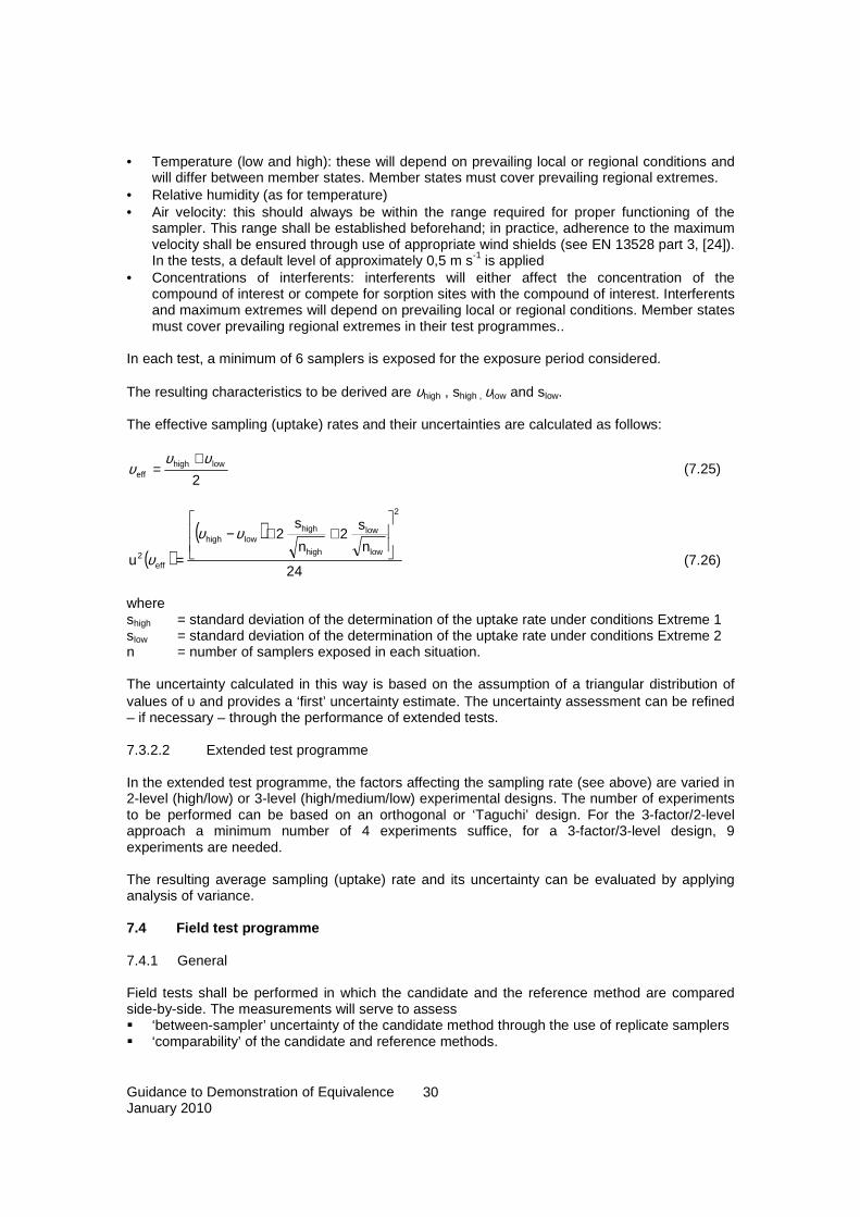
7.3.1.6 Evaluation of results of the laboratory tests The resulting WCM,lab is compared with the expanded relative uncertainty based on the data quality objective for the relevant species Wdqo. If WCM,lab ≤ Wdqo, the field test programme can be performed; if not, the candidate method shall first be improved, and relevant changes tested in the laboratory test programme. 7.3.2 Test Programme 1B. Diffusive sampling 7.3.2.1 Reduced test programme For general information about testing of diffusive samplers, the reader is referred to EN Standards EN 13528 parts 1-3 [23-25]. As a first estimate, the diffusive sampling flow (uptake rate) υ and its uncertainty can be determined under 2 sets of extreme conditions [26]. Extreme conditions for diffusive sampling are characterized by high and low extremes of sampling rates, depending on:
Guidance to Demonstration of Equivalence January 2010
30
• Temperature (low and high): these will depend on prevailing local or regional conditions and will differ between member states. Member states must cover prevailing regional extremes.
• Relative humidity (as for temperature) • Air velocity: this should always be within the range required for proper functioning of the
sampler. This range shall be established beforehand; in practice, adherence to the maximum velocity shall be ensured through use of appropriate wind shields (see EN 13528 part 3, [24]). In the tests, a default level of approximately 0,5 m s-1 is applied
• Concentrations of interferents: interferents will either affect the concentration of the compound of interest or compete for sorption sites with the compound of interest. Interferents and maximum extremes will depend on prevailing local or regional conditions. Member states must cover prevailing regional extremes in their test programmes..
In each test, a minimum of 6 samplers is exposed for the exposure period considered. The resulting characteristics to be derived are υhigh , shigh , υlow and slow. The effective sampling (uptake) rates and their uncertainties are calculated as follows:
2lowhigh
eff
υυυ
+= (7.25)
( )( )
24
n
s2
n
s2
u
2
low
low
high
highlowhigh
eff2
++−
=
υυ
υ (7.26)
where shigh = standard deviation of the determination of the uptake rate under conditions Extreme 1 slow = standard deviation of the determination of the uptake rate under conditions Extreme 2 n = number of samplers exposed in each situation. The uncertainty calculated in this way is based on the assumption of a triangular distribution of values of υ and provides a ‘first’ uncertainty estimate. The uncertainty assessment can be refined – if necessary – through the performance of extended tests. 7.3.2.2 Extended test programme In the extended test programme, the factors affecting the sampling rate (see above) are varied in 2-level (high/low) or 3-level (high/medium/low) experimental designs. The number of experiments to be performed can be based on an orthogonal or ‘Taguchi’ design. For the 3-factor/2-level approach a minimum number of 4 experiments suffice, for a 3-factor/3-level design, 9 experiments are needed. The resulting average sampling (uptake) rate and its uncertainty can be evaluated by applying analysis of variance. 7.4 Field test programme 7.4.1 General Field tests shall be performed in which the candidate and the reference method are compared side-by-side. The measurements will serve to assess � ‘between-sampler’ uncertainty of the candidate method through the use of replicate samplers � ‘comparability’ of the candidate and reference methods.

Guidance to Demonstration of Equivalence January 2010
31
Generally, results of existing studies, when demonstrably obtained according to the requirements of this test procedure, may be used to determine standard uncertainties. This is particularly relevant to the estimation of between-sampler/instrument uncertainties. In order to assure proper implementation of the reference method, two reference samplers or instruments may be used. In this case the mean squared difference of the results of both reference samplers/instruments can be used as an estimate of the (random) uncertainty of the reference method. The number of replicate samplers needed to determine the between-sampler uncertainty of the candidate method will depend on � the averaging period of the measurement � the practicability of performing multiple measurements in parallel � whether the analytical part of the candidate method is to be carried out by more than one
laboratory. Each laboratory carrying out analysis for the candidate method shall provide at least two samplers. When more than one laboratory will carry out the analysis, the field tests shall also be used to evaluate between-laboratory contributions to the uncertainty of the measurement results. 7.4.2 Experimental conditions Test sites shall be representative of typical conditions for which equivalence will be claimed, including possible episodes of high concentrations. A minimum of 4 comparisons shall be performed with particular emphasis on the following variables, if appropriate: � Composition of the air, notably high and low concentrations of the measured compound and
potential interferents � Air humidity and temperature (high and low) to cover any effects on sampling efficiency or
desorption efficiency � Wind speed (high and low) to cover any dependency of sampler performance due to
deviations from ideal behaviour. A minimum of 40 measurement results for the candidate method per comparison shall be collected over a minimum of 8 sampling periods covering a minimum of 20 days (e.g. 2 samplers and 20 periods, 5 samplers and 8 periods). Samplers and instruments shall be positioned in such a way that the effect of spatial inhomogeneity of the compound concentration in the sampled air is negligible in comparison with other uncertainty contributions. Both methods shall be operated under conditions reflecting practical application in the field, e.g., calibration intervals, flow checks, analysis of blank samples. During the tests, the following information shall be collected and recorded � Calibration procedures, equipment and intervals � (Results of) quality checks � Temperature and pressure of the sampled air � Other conditions relevant for the measurements performed (e.g., air humidity) � Particular events/situations that may be of influence on measurement results.
Guidance to Demonstration of Equivalence January 2010
32
7.4.3 Evaluation of the field test data 7.4.3.1 Conversion of measurement results to STP For the measurement of gaseous pollutants under [1] a conversion is required of measurement results to conditions of standard and pressure (STP, 20 °C, 101,3 kPa). Clause 7.3.1.1.3 describes the conversion and the assessment of the resulting uncertainty contribution. 7.4.3.2 Suitability of the dataset Of the full dataset at least 20% of the results shall be greater than or equal to the upper assessment threshold specified in [1]. Data shall only be removed from the data set when sound technical reasons can be found for doing so. All valid data shall be used for further evaluation. NOTE. Indications of outlying data within replicate sets may be obtained using Grubb’s tests on the individual single-period variances. Tests are to be performed at the 99% level. 7.4.3.3 Calculation of performance characteristics 7.4.3.3.1 Between-sampler/instrument uncertainty If the reference method is based on an AMS, the results for each measurement period i are averaged first to give values yi covering the same time periods as the exposure periods of the diffusive samplers. The relative between-sampler uncertainty for individual laboratories wbs is calculated from the differences of results of the candidate samplers/instruments operated in parallel as:
( )2
2n
1i2,i1,i
2bs
yn2
yyw
∑=
−= for duplicate samplers (7.27)
where yi,1 and yi,2 are the results of parallel measurements for a single period i
y = average of all measurement results of the candidate method n = number of measurement results.
( )( ) 2
n
1i
p
1j
2
ij,i2bs
y1pn
yy
w−
−=∑∑
= = for replicate samplers with p > 2 (7.28)
where yij = result of measurement j for a single period i
y i = mean result for period i p = number of replicates for period i. Where more than one analytical laboratory is participating, equation 7.28 shall be used to calculate the between-laboratory wbs.
Guidance to Demonstration of Equivalence January 2010
33
The wbs between sampler uncertainty component for each individual laboratory and the between-laboratory wbs (if relevant) shall comply with the criteria given in Annex A. If the performance of a single laboratory causes a method implemented by more than two laboratories to fail the criteria, then the results for this laboratory may be excluded, if sound technical grounds exist for doing so. 7.4.3.3.2 Comparison with reference method First, the performance of the reference samplers/instruments is checked by calculation of the relative between-sampler/instrument uncertainty as in eq. (7.27) or (7.28). This relative uncertainty shall be ≤ 3%. For the comparison of the candidate method with the reference method, first the results of replicate measurements are averaged to give data pairs ‘candidate method – reference method’ with equal measurement periods. For the evaluation of the uncertainty due to the ‘lack of comparability’ between candidate and reference method it is assumed that the relationship between measurement results of both methods can be described by a linear relation of the form
ii bxay += (7.29) where xi is the average result of the reference method over period i. The relation between the average results of the candidate method and those of the standard method is established using a regression technique that leads to a symmetrical treatment of both variables. A commonly applied technique is orthogonal regression [29]. The uncertainty due to lack of comparability will be a function of the concentration of the measurand. The general relationship describing the dependence of uCR on xi is given by
( ) ( ) ( ) ( )[ ]2ii2
i2CR x1baxu
2nRSS
yu −++−−
= (7.30)
where RSS = sum of (relative) residuals resulting from the orthogonal regression u(xi) = random uncertainty of the standard method. When two reference samplers/instruments have been used in the field test, u(xi) may be calculated as ubs,RM/√2 where ubs,RM is the reference between-sampler/instrument uncertainty calculated using eq. (7.27) with the duplicate reference results as input. Algorithms for the calculation of a and b and their variances are given in Annex B. RSS, the sum of (relative) residuals is calculated using eq. 7.31a or 7.32b, depending on whether the residuals or relative residuals are constant.
( )∑=
−−=n
1i
2ii bxayRSS when ( )2
ii bxay −− is constant (7.31a)
( )2
n
1i i
i2i 1
bxa
ybxaRSS ∑
=
−
++= when
2
i
i 1bxa
y
−
+is constant (7.31b)

Guidance to Demonstration of Equivalence January 2010
34
7.4.3.4 Calculation of the combined uncertainty of candidate method The combined relative uncertainty of the candidate method wc,CM is calculated by combining the contributions found in 7.4.3.2.1 and 7.4.3.2.2 as follows:
( ) ( )2i
i2CR
i2
CM,cy
yuyw = (7.32)
In this way, wc,CM is expressed as a function of the compound concentration. The uncertainty at the limit value wCM is calculated by taking as yi the concentration at the limit value. 7.4.3.5 Calculation of the expanded uncertainty of candidate method The expanded relative uncertainty of the results of the candidate method is calculated by multiplying wc,CM by a coverage factor k reflecting the appropriate number of degrees of freedom resulting from the determination of wc,CM as
CM,cfield,CM wkW ⋅= (7.33)
In view of the large number of experimental results available, a coverage factor k=2 can be used for a 95% confidence level. 7.4.4 Evaluation of results of field tests The resulting uncertainty estimate WCM is compared with the expanded relative uncertainty obtained from the laboratory test programme WCM,l and the expanded relative uncertainty based on the data quality objective for the standard method Wdqo. In principle, three cases are possible 1. WCM,field ≤ WCM,lab: the candidate method is accepted as equivalent to the reference method 2. WCM,lab < WCM,field ≤ Wdqo : the candidate method is accepted conditionally; before final
acceptance, the uncertainty evaluation from the laboratory tests should be revisited and corrected such that situation 1 occurs
3. WCM,field > Wdqo: the candidate method is not accepted as equivalent method.

Guidance to Demonstration of Equivalence January 2010
35
8 TEST PROGRAMME 2 - AUTOMATED MEASUREMENT SYSTEMS FOR GASES 8.1 General This test programme describes a procedure for determining whether a candidate method is suitable to be considered equivalent to the reference method for the measurement of gases and vapours in ambient air using automated measurement systems. This test programme covers the requirements for the equivalence testing of an AMS where it is practical to achieve measurements that have full traceability to SI units. These include continuous ambient-air analysers monitoring sulphur dioxide, the nitrogen oxides (NO and NO2) ozone and carbon monoxide. Analysers measuring benzene in ambient air by sequential automated (quasi–continuous) sampling and subsequent measurements by gas chromatography are also covered. The use of similar automated methods for the measurement of precursor ‘non-methane hydrocarbons’ discussed in EU Directive 2008/50/EC [1] are not included because these measurements are not covered by an EN standard method, nor are there yet any assigned uncertainty requirements for such methods. The methodology specified in this section for equivalence testing follows very closely the procedures specified in the appropriate EN standards prepared by CEN Technical Committee 264 ‘Air Quality’. 8.2 Overview of the test procedures The reference methods specify procedures for the type-approval testing of analysers to determine whether their performance (overall measurement uncertainty, data capture etc) conforms to the requirements of [1]. These tests define all the individual performance characteristics which contribute to the combined uncertainty of the method (repeatability, responses to cross interferents etc), and which therefore shall be tested. The reference methods also specify minimum (performance) criteria to which the individual performance characteristics shall conform. In addition, the EN standards specify procedures to determine the expanded uncertainty of the method from the component performance criteria obtained during tests, and this expanded uncertainty shall be compared with the expanded uncertainty data quality objective given in [1], in order to assess the performance of the analyser with respect to the Directive’s requirements. Therefore, a candidate method will be treated as a ‘black box’ measurement system and will undergo testing to determine the uncertainty introduced by all the different performance characteristics of the complete measurement system. These separate uncertainties shall then be combined to give an expanded uncertainty, expressed with a level of confidence of 95%, for the CM, which shall then comply with the measurement uncertainty laid down in [1]. Testing shall be carried out in two parts: a laboratory test in which two instruments of the same pattern will be tested, and a field test in which these two instruments will be tested together against the relevant reference method. If a CM is a modification to an existing type-approved analyzer, then only the laboratory performance characteristics that are affected by the modification shall be tested and their standard uncertainties calculated. The standard uncertainties associated with unaffected performance characteristics shall then be used together with these existing standard uncertainties, to determine the combined measurement uncertainty, uc. An example of such a modification would be a new material for a converter of NOx to NO within a chemiluminescence

Guidance to Demonstration of Equivalence January 2010
36
NOx analyzer. Under this modification only the converter efficiency test and the response time test shall be performed in the lab tests. In all cases the field tests shall be performed. If a CM utilises a measurement method that is different to the EN standard method, then all of the tests shall be performed. The following performance characteristics of the CM will be tested, where applicable: (i) Laboratory tests � response time, consisting of rise lag time, rise time, fall lag time and fall time (where
applicable); � laboratory repeatability standard deviation; � short-term zero and span drift; � difference between sample port and calibration port (where applicable); � detection limit ; � averaging of short-term fluctuations in measurand concentration (where applicable); � lack of fit (linearity); � cross-sensitivity to potentially-interfering substances; � NOx converter efficiency test (where applicable); � carry-over (where applicable); � influence of atmospheric sample pressure and temperature; � influence of surrounding air temperature � influence of supply voltage variations. Both analysers used in the laboratory tests are required to pass all the tests. (ii) Field tests � field performance of two CM analysers of the same type(pattern) against the relevant
standard method to determine whether systematic differences occur in the measured results; � field repeatability of two CM analysers; � long-term zero and span drift; � availability (maintenance interval). Both analysers used in the field tests are required to pas all the tests. The performance characteristics calculated from the tests shall be compared to the same performance characteristics defined in Table 3. From the performance characteristics the following standard uncertainties, where applicable, shall be calculated and used to calculate the combined expanded measurement uncertainty of the CM: Table 3. Uncertainty components to be included in the combined standard measurement uncertainty
Uncertainty Source Symbol Repeatability at zero uz Repeatability at 70-80% of the certification concentration us Between-instrument uncertainty uf Carry over uc Lack of fit (linearity) ul Difference between sample and calibration port ua Effect of short term fluctuations in concentration uav Cross sensitivity to interfering substances uH2O, uint
Variation in sample pressure up

Guidance to Demonstration of Equivalence January 2010
37
Variation in sample temperature ut Variation in surrounding air temperature ust
Variation in supply voltage uv NOx converter efficiency uce Comparison with the standard method UCM Long-term zero drift uzd Long-term span drift usd 8.3 Definitions applicable to automated measurement sys tems 8.3.1 Independent measurement
An individual measurement that is not influenced by a previous individual measurement, by separating two individual measurements by at least four response times.
8.3.2 Individual measurement
A measurement averaged over a time period equal to the response time of the analyser.
8.4 Laboratory tests 8.4.1 Test concentrations Laboratory tests are performed, in principle, over the range of concentrations specified in the EN standard describing the reference method. A more restricted certification range may be selected by a Member State if judged appropriate. (The CM will then only be applicable to results obtained in this restricted certification range.) Test concentrations specified here for the laboratory tests are based on the maximum of the selected certification range, unless specified otherwise. 8.4.2 Response time The tests of response time shall be performed on all candidate methods that give approximately real-time measurements. For instruments such as gas chromatographs, the concept of response time is inappropriate and the response time shall be taken to be the time interval of the sampling. For example, if the instrument collects a sample once an hour, then the assumed response time will be one hour. The requirement on response time for this type of CM is that the assumed response time is less than 25% of the required averaging period. For real-time CMs the following test procedure shall be used: Apply a step change of gas concentration to the CM. The step change value shall be within 20% and 80% of the maximum of the certification range of the CM and will normally be to 80%, and need not start from or end at zero concentration. The applied change of concentration must reach 90% of the full change of value within 10 seconds of the start of the change. Record the response of the CM to the applied step change of concentration and determine the lag time (the time taken by the CM to indicate 10% of the final concentration value), the response time (the time taken for the CM to indicate 90% of the final concentration value) and the rise time (the difference between the response time and the lag time). Measurements will be made with at least four step changes of concentration in both positive and negative directions. As well as calculating the individual rise and fall response times the relative difference in response times will also be calculated. When the reading of 98 % of the applied concentration has been reached, the span gas can be changed to zero again. This event is the start (t = 0) of the (fall) lag time. When the reading of
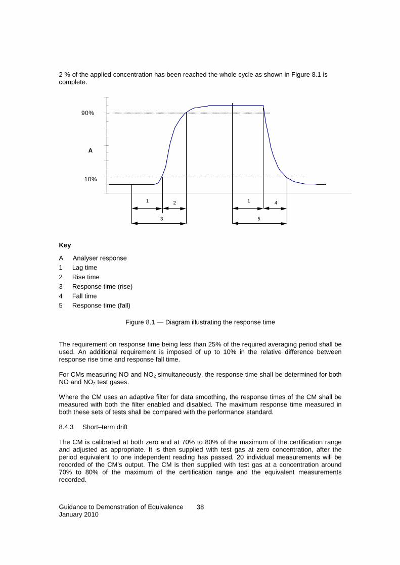
Guidance to Demonstration of Equivalence January 2010
38
2 % of the applied concentration has been reached the whole cycle as shown in Figure 8.1 is complete.
10%
90%
1 2
3 5
1 4
A
Key
A Analyser response
1 Lag time
2 Rise time
3 Response time (rise)
4 Fall time
5 Response time (fall)
Figure 8.1 — Diagram illustrating the response time
The requirement on response time being less than 25% of the required averaging period shall be used. An additional requirement is imposed of up to 10% in the relative difference between response rise time and response fall time. For CMs measuring NO and NO2 simultaneously, the response time shall be determined for both NO and NO2 test gases. Where the CM uses an adaptive filter for data smoothing, the response times of the CM shall be measured with both the filter enabled and disabled. The maximum response time measured in both these sets of tests shall be compared with the performance standard. 8.4.3 Short–term drift The CM is calibrated at both zero and at 70% to 80% of the maximum of the certification range and adjusted as appropriate. It is then supplied with test gas at zero concentration, after the period equivalent to one independent reading has passed, 20 individual measurements will be recorded of the CM’s output. The CM is then supplied with test gas at a concentration around 70% to 80% of the maximum of the certification range and the equivalent measurements recorded.

Guidance to Demonstration of Equivalence January 2010
39
The CM shall be operated under the laboratory conditions whilst analysing ambient air. After a minimum period of 12 hours the repeatability test is repeated. The averaged values obtained for zero and 70% to 80% of the maximum of the certification range shall be calculated. This test shall be used to show that the 12-hour drift is not the dominant factor in any of the test results. The short-term drift at zero and at 70% to 80% of the maximum of the certification range shall be calculated as follows:
( )1,z2,zz,s CCD −= (8.1)
where
Ds,z = the 12-hour drift at zero;
Cz,1 = the average of the zero gas measurements at the beginning of the drift period (just after calibration); Cz,2 = the average of the zero gas measurements at the end of the drift period (12 hours).
Dsz shall comply with the performance criterion for short term drift at zero given in the relevant EN Standard for the measurand.
( )1,2,, ssss CCD −=
Span drift now zero drift corrected
( ) zsssss DCCD ,1,2,, −−= (8.2)
where: Ds,s = the 12-hour drift at the test concentration Ct (nmol/mol); Cs,1 = the average of the span gas measurements at the beginning of the drift period (just after calibration) (nmol/mol); Cs,2 = the average of the span gas measurements at the end of the drift period (12 hours) (nmol/mol) Ds,s shall comply with the performance criterion for short term drift at span levels given in the relevant EN Standard for the compound under investigation. 8.4.4 Repeatability for continuous measuring CMs Test gases shall be supplied to the CM at zero concentration and the highest numerical limit or target value specified for the pollutant for a period equivalent to one independent measurement, and then 20 individual measurements of the CM’s output are recorded. From these measurements the repeatability standard deviation (si) at zero concentration and at concentration ct shall be calculated according to:
( )1
2
i -
-‡”n
yys
i= (8.3)
where:
si = the repeatability standard deviation; yi = the ith measurement;
y = the average of the 20 measurements;

Guidance to Demonstration of Equivalence January 2010
40
n = the number of measurements, n =20.
The repeatability standard deviation shall be calculated separately for both series of measurements (zero gas and concentration ct) and the repeatability (ri) is calculated according to:
i05.0,1ni str ⋅= (8.4)
where: tn-1, 0,05 = the two-sided Students t-factor at a confidence level of 0,05, with n-1 degrees of freedom (for n = 20, tn-1, 0,05 = 2,09); sl = the repeatability standard deviation.
rl shall comply with the performance criteria for repeatability at zero and repeatability at the limit value concentration, respectively, given in the EN standard for the measurand. The standard uncertainties uz and us, for repeatability are equal to the repeatability standard deviation, sl, calculated above, for the zero and the limit/target value concentrations. 8.4.5 Carry over and repeatability for CMs collecting samples onto a sorbent prior to analysis CMs that collect samples by absorption or other similar means and then subsequently analyse them shall be tested for the carry-over of measurand from one sample to the next. The CM shall be supplied with test gas for one sampling period, at the highest numerical limit or target value specified for the pollutant, followed by one sampling period of zero gas. This procedure shall be repeated 20 times and the results shall be used to calculate both the repeatability standard deviation at the limit value concentration and the carry over standard deviation according to:
( )1
2
i -
-‡”n
yys
i= (8.5)
where: si = the repeatability / carry over standard deviation; yi = the ith measurement ;
y = the average of the 20 measurements; n = the number of measurements, n =20. The repeatability standard deviation shall be calculated separately for both series of measurements (zero gas and concentration ct) and the repeatability (ri) is calculated according to eq. (8.4). rl shall comply with the performance criteria for carry over and repeatability specified in the relevant EN Standard, respectively. The standard uncertainties uc and us, for carry over and repeatability are equal to the repeatability standard deviation, si calculated above, for the carry over and limit value test concentrations. 8.4.6 Lack of fit (linearity) The CM shall be adjusted at a concentration of about 90 % of the maximum of the certification range. The linearity of the CM shall then be tested over the range 0 % to 95 % of the maximum of the certification range of the CM using at least 6 concentrations (including the zero point). At each concentration (including zero) at least 5 independent readings shall be performed.

Guidance to Demonstration of Equivalence January 2010
41
The concentrations shall be applied in the following sequence: 80 %, 40 %, 0 %, 60 %, 20 % and 95 %. The dilution ratios for the applied concentrations shall be less than 1,5 % with respect to each other. Continuous measuring CMs After each change in concentration a delay of at least 4 response times shall be taken into account before the next measurement is performed. Non-continuous measuring CMs After each change in concentration at least a delay of 1 response time shall be taken into account before the next measurement is performed. For both, a linear regression function is calculated from the measured mean responses at each concentration. The relative residual for each measured concentration is calculated. The largest relative residual ρmax and the actual residual at the zero concentration will be compared against the performance criteria for lack of fit. The standard uncertainty due to the lack of fit at the limit value concentration, ul, is calculated according to:
3max LV
u l
⋅=
ρ (8.6)
where: ul = the standard uncertainty due to lack of fit at the limit value concentration; LV = the highest numerical limit or target value specified for the pollutant.
8.4.7 Difference between sample and calibration port If the CM has different ports for sample gas and calibration gas, the difference in response of the CM when test gas is introduced through the sample or calibration port shall be tested. The test shall be carried out by supplying test gas, with a concentration of 70 % to 80 % of the maximum of the certification range, through the sample port for a time period equal to one independent measurement. Three individual measurements shall then be taken of the CM output. Zero gas is then supplied to the sample port for a time period equal to one independent measurement. This test is repeated with the teat gas supplied to the calibration port instead of the sample port. A delay of 4 response times should be left between testing the sample and calibration ports to allow for flushing. The difference shall be calculated according to:
100%t
cssc ×
−=
c
yyD (8.7)
where
Dsc = the difference sample/calibration port (%);
ys = the average of the concentrations measured using the sample port;
yc = the average of the concentrations measured using the calibration port;
ct = the concentration of the test gas.
Guidance to Demonstration of Equivalence January 2010
42
Dsc shall comply with the performance criterion for the difference between the sample and calibration port in the relevant EN standard for the compound under investigation. The standard uncertainty due to the difference between the sample and calibration port, ua, is calculated according to:
3
LV100D
u
sc
a
⋅= (8.8)
where ua = the standard uncertainty due to the difference between the sample and calibration ports, at the highest numerical limit or target value specified for the pollutant. 8.4.8 Effect of short-term fluctuations in concentration (averaging test) The averaging test gives a measure of the uncertainty in the averaged values caused by concentration variations in the sampled air shorter than the time scale of the measurement process in the analyser. For the determination of the uncertainty due to the averaging the following concentrations are applied to the analyser and readings are taken at each concentration: 1) CO, O3, SO2 and benzene measuring CMs - a constant concentration of the measurand at a concentration that is about twice the
highest numerical limit value specified for the pollutant - a stepwise varied concentration of the measurand between zero and about twice the
highest numerical limit value specified for the pollutant. 2) CMs measuring NO and NO2 simultaneously - a constant concentration of NO2 at a concentration, which is about the hourly limit value; - a stepwise varied concentration of NO between zero and a concentration corresponding
to about six times the hourly limit value for NO2. For non-continuously measuring CMs the time period (tc) of the constant concentration shall be at least equal to a period necessary to obtain two cycle periods (which equals to at least two response times). The time period (tv) of the varying concentration shall be at least equal to to a period necessary to obtain four cycle periods (which equals to at least four response times). The time period (tD) for the measurand concentration shall be 90 seconds followed by a period (tzero) of 90 seconds of zero concentration.
The change from tD to tzero shall be within 0,5 seconds. The change from tC to tV shall be within one response time of the analyser under test. The averaging effect (Xav) is calculated according to:
%100C
C2CX
avconst
avvar
avconst
av ××−
= (8.9)
where Xav = the averaging effect (%);
avconstC = the average of the at least 4 independent measurements during the constant
concentration period (tc);

Guidance to Demonstration of Equivalence January 2010
43
avvarC = the average of the at least 4 independent measurements during the variable
concentration period (tv). Xav shall comply with the requirements for the measurand in the relevant EN standard. For instruments measuring NO and NO2 simultaneously, Xav shall be calculated for both channels and compared with these requirements. The resulting uncertainty uav is calculated as
3100
Xu av
av = (8.10)
8.4.9 Variation in sample-gas pressure Measurements are taken at a concentration of about 70 % to 80 % of the maximum of the certification range of the CM at an absolute pressure of about 80 kPa ± 0,2 kPa and at an absolute pressure of about 110 kPa ± 0,2 kPa. At each pressure the test gas is supplied for a time period equal to one independent measurement and then three individual measurements will then be taken of the CMs output. From these measurements the averages at each pressure are calculated. Measurements at different pressures shall be separated by at least 4 response times for continuous measuring CMs and one response time for non-continuous measuring CMs. The sensitivity coefficient for the influence of sample gas pressure is calculated by:
12
1PP2
PP
CC=
P
C
−−
∆
∆ (8.11)
where
1CP = the average concentration of the measurements at sampling gas pressure P1;
2CP = the average concentration of the measurements at sampling gas pressure P2;
P1 = the sampling gas pressure P1 (kPa); P2 = the sampling gas pressure P2 (kPa). The test parameter bgp to be compared to the test criterion in the relevant EN standard for the compound investigated is then calculated as
tgp C
100
P
Cb ⋅=
∆
∆
(8.12) where Ct is the applied test gas concentration. The standard uncertainty due sample pressure variation, up, is calculated according to:
3
PP
PC
u minmaxp
−⋅=
∆
∆ (8.13)
where Pmax and Pmin are the extremes of pressures encountered in practice.

Guidance to Demonstration of Equivalence January 2010
44
For calculation of the standard uncertainty from the results of the type-approval test, Pmax and Pmin equal P2 and P1, respectively. 8.4.10 Variation in sample-gas temperature For the determination of the dependence of the sample gas temperature measurements shall be performed at sample gas temperatures of 0 °C and 30 °C. The temperature dependence shall be determined at a concentration of about 70 % to 80 % of the maximum of the certification range of the CM. At each temperature the test gas is supplied for a time period equal to one independent measurement and then three individual measurements will then be taken of the CMs output. The sample gas temperature, measured at the inlet of the analyser, shall be held constant for at least 30 minutes before any measurements are taken. The sensitivity coefficient for the influence of sample gas temperature is calculated as:
12
1T2T
sg TT
CC
T
C
−−
=∆∆
(8.14)
where
1TC = the average concentration of the measurements at sample gas temperature T1 (°C);
2TC = the average concentration of the measurements at sample gas temperature T2 (°C);
T1 = the sample gas temperature T1 (°C); T2 = the sample gas temperature T2 (°C). The test parameter bgp to be compared to the test criterion in the relevant EN standard for the compound investigated is then calculated as
tsgsg C
100
T
Cb ⋅=
∆
∆ (8.15)
where Ct is the applied test gas concentration. The standard uncertainty due sample pressure variation, up, is calculated according to:
3
TT
TC
u min,sgmax,sg
sgp
-∆ ⋅=∆
(8.16)
where Tsg,max and Tsg,min are the extremes of temperature encountered in practice. For calculation of the standard uncertainty from the results of the type-approval test, Tmax and Tmin equal T2 and T1, respectively. 8.4.11 Surrounding temperature variation The influence of the surrounding air temperature shall be determined at the following temperatures (within the specifications of the manufacturer): � the minimum specified temperature (Te,min); � at the laboratory temperature (T1); � at the maximum specified temperature (Te,max). For these tests a climate chamber is necessary.
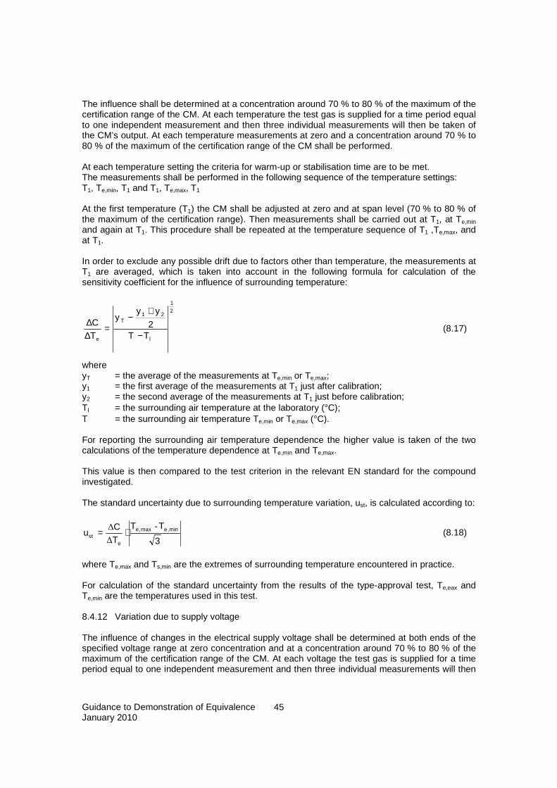
Guidance to Demonstration of Equivalence January 2010
45
The influence shall be determined at a concentration around 70 % to 80 % of the maximum of the certification range of the CM. At each temperature the test gas is supplied for a time period equal to one independent measurement and then three individual measurements will then be taken of the CM’s output. At each temperature measurements at zero and a concentration around 70 % to 80 % of the maximum of the certification range of the CM shall be performed. At each temperature setting the criteria for warm-up or stabilisation time are to be met. The measurements shall be performed in the following sequence of the temperature settings: T1, Te,min, T1 and T1, Te,max, T1 At the first temperature (T1) the CM shall be adjusted at zero and at span level (70 % to 80 % of the maximum of the certification range). Then measurements shall be carried out at T1, at Te,min and again at T1. This procedure shall be repeated at the temperature sequence of T1 ,Te,max, and at T1. In order to exclude any possible drift due to factors other than temperature, the measurements at T1 are averaged, which is taken into account in the following formula for calculation of the sensitivity coefficient for the influence of surrounding temperature:
2
1
l
21T 2
TT
yyy
TC
e −
+−
=∆∆
(8.17)
where yT = the average of the measurements at Te,min or Te,max; y1 = the first average of the measurements at T1 just after calibration; y2 = the second average of the measurements at T1 just before calibration; Tl = the surrounding air temperature at the laboratory (°C); T = the surrounding air temperature Te,min or Te,max (°C).
For reporting the surrounding air temperature dependence the higher value is taken of the two calculations of the temperature dependence at Te,min and Te,max. This value is then compared to the test criterion in the relevant EN standard for the compound investigated. The standard uncertainty due to surrounding temperature variation, ust, is calculated according to:
3
TT
TC
u min,emax,e
est
-
∆
∆ ⋅= (8.18)
where Te,max and Ts,min are the extremes of surrounding temperature encountered in practice. For calculation of the standard uncertainty from the results of the type-approval test, Te,eax and Te,min are the temperatures used in this test. 8.4.12 Variation due to supply voltage The influence of changes in the electrical supply voltage shall be determined at both ends of the specified voltage range at zero concentration and at a concentration around 70 % to 80 % of the maximum of the certification range of the CM. At each voltage the test gas is supplied for a time period equal to one independent measurement and then three individual measurements will then

Guidance to Demonstration of Equivalence January 2010
46
be taken of the CMs output. At each voltage measurements at zero and around 70 % to 80 % of the maximum of the certification range shall be performed. The sensitivity coefficient for the influence of voltage dependence is calculated according to:
12
1V2V
VV
CC
V
C
−−
=∆∆
(8.19)
where
1VC = the average concentration reading of the measurements at voltage V1;
2VC = the average concentration reading of the measurements at voltage V2;
V1 = the minimum voltage Vmin (V) specified by the manufacturer; V2 = the maximum voltage Vmax (V) specified by the manufacturer.
For reporting the dependence on voltage the highest value of the result at zero and span level shall be taken. This value is then compared to the test criterion in the relevant EN standard for the compound under investigation. For an analyser operating on direct current the type approval test of voltage variation shall be carried out over the range of ± 10 % of the nominal voltage. The standard uncertainty due to voltage variation, uv, shall be calculated according to:
3
VV
VC
u minmaxv
−⋅=
∆∆
(8.20)
where Vmax and Vmin are the extremes of line voltage encountered in practice. For calculation of the standard uncertainty from the results of the type-approval test, Vmax and Vmin equal V2 and V1, respectively. 8.4.13 Cross-sensitivity to interfering substances The analyser’s response to certain interfering substances, which are to be expected to be present in ambient air and which may also interfere with the CMs measurement process shall be tested. These interferents can give a positive or negative response. The test shall be performed at zero and at a test concentration (ct) similar to the highest numerical limit or target value specified for the pollutant. The concentration of the mixtures of the test gases with the interferent shall have an uncertainty of less than 5 % and shall be traceable to (inter)nationally accepted standards. The influence of each interferent shall be determined separately. A correction on the concentration of the measurand shall be made for the dilution effect due to addition of an interferent (e.g. water vapour). After adjustment of the analyser at zero and 70% to 80% of the maximum of the certification range the analyser shall be fed with a mixture of zero gas and the interferent to be investigated. This mixture will be supplied for a time period equal to one independent measurement, and, following this, three individual measurements will then be taken of the CMs output. This procedure shall be repeated with a mixture of the measurand at concentration ct and the interferent to be investigated. The influence quantity at zero and concentration ct are calculated from:

Guidance to Demonstration of Equivalence January 2010
47
zzint, = yY (8.21)
where Yint, z = the influence quantity of the interferent at zero; yz = the average of the measurements at zero. and:
ttctcint, -y=Y c (8.22)
where
tcint,Y = the influence quantity of the interferent at concentration ct;
tcy = the average of the measurements at concentration ct;
ct = the concentration of the applied gas at the level of the hourly limit value. The standard uncertainties due to interfering substances, uH2O and uint, are calculated as follows. The influence quantity of water vapour is established at a water concentration of 19 mmol/mol. The uncertainty, however, is to be established at a water concentration of 21 mmol/mol. The standard uncertainty due to interference by the presence of water vapour at the highest numerical limit value specified for the pollutant, uH2O, is therefore calculated according to:
zO,2Hmaxz,O,2H Y)19/21(Y = (8.23)
tcO,2Hmax,tcO,2H Y)19/21(Y = (8.24)
maxz,O,2Htmaxz,O,2Hmax,tcO,2HmaxO,2H )/)(( YLVcYYY +⋅= - (8.25)
3/)(/ 2minO,2HminO,2HmaxO,2H
2maxO,2HmaxO,2HO2HO2H cccccYu ++⋅= (8.26)
where
maxz,O,2HY = the influence quantity of an H2O concentration of 21 mmol/mol at zero concentration of
the measurand (nmol/mol);
zO,2HY = the influence quantity of an H2O concentration of 19 mmol/mol at zero concentration of
the measurand (nmol/mol);
max,tcO,2HY = the influence quantity of an H2O concentration of 21 mmol/mol at the test
concentration ct of the measurand (nmol/mol);
tcO,2HY = the influence quantity of an H2O concentration of 19 mmol/mol at the test concentration
ct of the measurand (nmol/mol);
O2HY = the influence quantity of an H2O concentration of 21 mmol/mol at the hourly limit value
(nmol/mol);
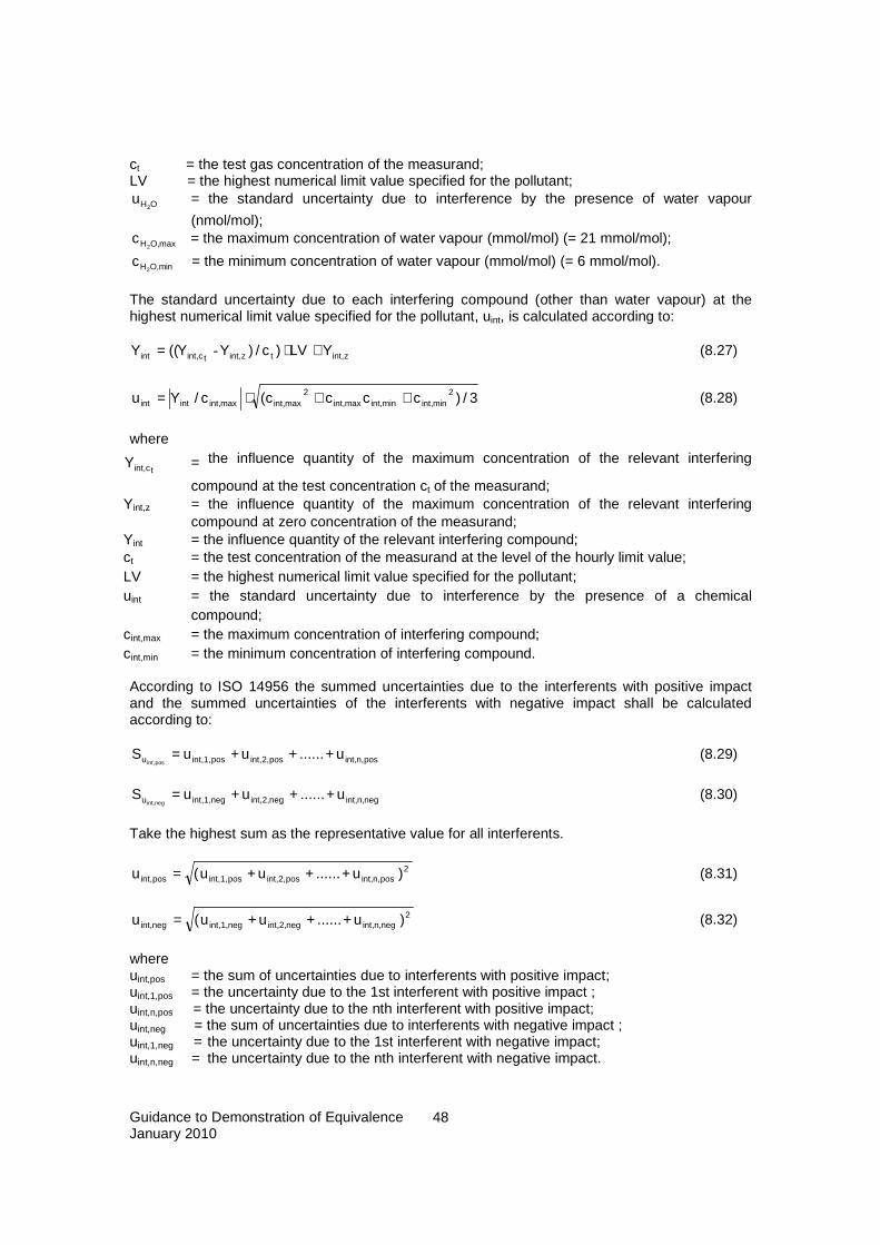
Guidance to Demonstration of Equivalence January 2010
48
ct = the test gas concentration of the measurand; LV = the highest numerical limit value specified for the pollutant;
OH2u = the standard uncertainty due to interference by the presence of water vapour
(nmol/mol);
maxO,H2c = the maximum concentration of water vapour (mmol/mol) (= 21 mmol/mol);
minO,H2c = the minimum concentration of water vapour (mmol/mol) (= 6 mmol/mol).
The standard uncertainty due to each interfering compound (other than water vapour) at the highest numerical limit value specified for the pollutant, uint, is calculated according to:
zint,tzint,tcint,int )/)(( YLVcYYY +⋅= - (8.27)
3/)(/ 2minint,minint,maxint,
2maxint,maxint,intint cccccYu ++⋅= (8.28)
where
tcint,Y = the influence quantity of the maximum concentration of the relevant interfering
compound at the test concentration ct of the measurand; Yint,z = the influence quantity of the maximum concentration of the relevant interfering
compound at zero concentration of the measurand; Yint = the influence quantity of the relevant interfering compound; ct = the test concentration of the measurand at the level of the hourly limit value; LV = the highest numerical limit value specified for the pollutant; uint = the standard uncertainty due to interference by the presence of a chemical
compound; cint,max = the maximum concentration of interfering compound; cint,min = the minimum concentration of interfering compound. According to ISO 14956 the summed uncertainties due to the interferents with positive impact and the summed uncertainties of the interferents with negative impact shall be calculated according to:
posn,int,posint,2,posint,1,u u......uuSposint,
+++= (8.29)
negn,int,negint,2,negint,1,u u......uuSnegint,
+++= (8.30)
Take the highest sum as the representative value for all interferents.
2posn,int,posint,2,posint,1,posint, )u......uu(u +++= (8.31)
2negn,int,negint,2,negint,1,negint, )u......uu(u +++= (8.32)
where uint,pos = the sum of uncertainties due to interferents with positive impact; uint,1,pos = the uncertainty due to the 1st interferent with positive impact ; uint,n,pos = the uncertainty due to the nth interferent with positive impact; uint,neg = the sum of uncertainties due to interferents with negative impact ; uint,1,neg = the uncertainty due to the 1st interferent with negative impact; uint,n,neg = the uncertainty due to the nth interferent with negative impact.

Guidance to Demonstration of Equivalence January 2010
49
8.4.14 NO2 converter efficiency The converter efficiency is determined by measurements with calculated amounts of NO2. This can be achieved by means of gas-phase titration of NO to NO2 with ozone. The test is to be performed at two concentration levels: at 50 % and 95 % of the maximum of the certification range of NO2. The NOx analyser shall be calibrated on the NO and NOx channel with a NO concentration around 70 % to 80 % of the maximum of the certification range of NO. Both channels shall be set to read the same value and the values shall be recorded. A known concentration of about 50 % of the maximum of the certification range of NO shall be supplied to the analyser until a stable output signal is achieved. This stabilisation period shall be at least four times the response time of the analyser. Four individual measurements are taken at the NO and NOx channel. The NO will then be reacted with O3 to produce the required concentration of NO2, the NO residue after the gas phase titration reaction shall be 10 % to 20 % of the original NO concentration. This mixture with a constant NOx concentration shall be supplied to the analyser until a stable output signal is achieved. This stabilisation period shall be at least four times the response time of the analyser. Four individual measurements are then taken at the NO and the NOx channel. The O3 supply shall be switched off and the analyser supplied with only NO until a stable output signal is achieved. This stabilisation period shall be at least four times the response time of the analyser. Then the average of the four individual measurements at the NO and NOx channel is checked to see whether it is equal within 1 % of the original values. Repeat the test with a NO test concentration of approximately 95% of the maximum of the certification range of NO2. Calculate the converter efficiency from:
( ) ( )( ) ( ) %100 ×
fNO-iNOfxNO-ixNO
-1=convE
(8.33)
where Econv = the converter efficiency in %; (NOx)i = the average of the four individual measurements at the NOx channel at the initial NOx
concentration; (NOx)f = the average of the four individual measurements at the NOx channel at the resulting
NOx concentration after applying O3; (NO)i = the average of the four individual measurements at the NO channel at the initial NO
concentration; (NO)f = the average of the four individual measurements at the NO channel at the resulting NO
concentration after applying O3.
The lowest value of the two converter efficiencies shall be used to calculate the standard
uncertainty due to converter efficiency, uce, according to:
LV3100
Eu conv
ce ⋅= (8.34)

Guidance to Demonstration of Equivalence January 2010
50
where LV is the highest numerical limit value specified for the pollutant. 8.5 Field test
8.5.1 General In the field test two CMs of the same type (pattern) are tested for availability (period of unattended operation), between-instrument uncertainty and long-term drift. The CMs are run in parallel at one and the same sampling point at a selected monitoring station. Operational requirements are given below for the correct determination of the long-term drift and the between-instrument uncertainty. The reference method will be operated alongside the two CMs, with parallel measurements from one and the same sampling point. From these results any systematic differences between the results obtained by the CM and the reference method will be determined. 8.5.2 Experimental conditions Test sites shall be representative for typical conditions for which equivalence will be claimed, including possible episodes of high concentrations. A minimum of 4 comparisons shall be performed with particular emphasis on the following variables, if appropriate: � Composition of the air, notably high and low concentrations of the measured compound and
potential interferents � Air humidity and temperature (high and low) to cover any effects on sampling efficiency or
desorption efficiency � Wind speed (high and low) to cover any dependency of sampler performance due to
deviations from ideal behaviour. Each comparison shall cover a minimum of one month of uninterrupted monitoring during which hourly-average measurement results shall be collected. Both methods shall be operated under conditions reflecting practical application in the field, e.g., calibration intervals, appropriate span and zero checks. At the beginning of the test both CMs will be adjusted to read the same value. During the tests, the following information shall be collected and recorded � calibration procedures, equipment and intervals � (results of) quality checks � temperature and pressure of the sampled air � other conditions relevant for the measurements performed (e.g., air humidity) � particular events/situations that may be of influence on measurement results.
8.5.3 Evaluation of data collected 8.5.3.1 Suitability of datasets Of the full dataset at least 20% of the results shall be greater than or equal to the upper assessment threshold for the highest limit or target specified in [1]. Data shall only be removed from the data set when sound technical reasons can be found for doing so. All valid data shall be used for further evaluation. NOTE. Indications of outlying data (pairs) may be obtained using Grubb’s tests on the individual single-period variances. Outlier tests are to be performed at the 99% level.

Guidance to Demonstration of Equivalence January 2010
51
8.5.3.2 Between-instrument uncertainty The relative between-sampler/instrument uncertainty wbs is calculated from the differences of all hourly results of the candidate samplers/instruments operated in parallel as:
( )2
n
1i
22,i1,i
2bs
yn2
yyw
∑=
−= (8.35)
where yi,1 and yi,2 are the results of parallel measurements for a single 1-hour period i n = number of hourly measurement results
y = average of all measurement results of the candidate method. The between-instrument uncertainty shall comply with the criterion given in Annex B. 8.5.3.3 Comparison with the standard method For a comparison with the standard method the results of the parallel measurements of reference samplers/instruments and candidate samplers/instruments are averaged to give one result xi or yi for common measurement periods of equal length. For the evaluation of the uncertainty due to the ‘lack of comparability’ between candidate and standard methods it is assumed that the relationship between measurement results of both methods can be described by a linear relation of the form
ii bxay += (8.36) The relation between the average results of the candidate method and those of the standard method is established using a regression technique that leads to a symmetrical treatment of both variables. A commonly applied technique is orthogonal regression [27]. The uncertainty due to lack of comparability will be a function of the concentration of the measurand. The general relationship describing the dependence of uCR on xi is given by
( ) ( ) ( ) ( )[ ]2ii2
i2CR x1baxu
2nRSS
yu −++−−
= (8.37)
where RSS = the sum of (relative) residuals resulting from the orthogonal regression u(xi) = random uncertainty of the standard method. When two reference samplers/instruments have been used in the field test, u(xi) may be calculated as ubs,RM/√2 where ubs,RM is the reference between-sampler/instrument uncertainty calculated using eq. (8.35) with the duplicate reference results as input. Algorithms for the calculation of a and b and their variances are given in Annex C. RSS, the sum of (relative) residuals is calculated using eq. 8.38a or 8.38b, depending on whether the residuals or relative residuals are constant.
( )∑=
−−=n
1i
2ii bxayRSS when ( )2
ii bxay −− is constant (8.38a)

Guidance to Demonstration of Equivalence January 2010
52
( )2
n
1i i
i2i 1
bxa
ybxaRSS ∑
=
−
++= when
2
i
i 1bxa
y
−
+is constant (8.38b)
8.5.3.3 Calculation of the combined ’field’ uncertainty to be assigned to the candidate method The combined relative field uncertainty of the candidate method wCM,field is calculated by combining the contributions found in 8.5.3.1 and 8.5.3.2 as follows:
( ) ( )2i
i2CR
i2
field,CMy
yuyw = (8.39)
The uncertainty at the limit value with the shortest averaging period, wCM,field, is calculated by taking as yi the concentration at the limit value. 8.5.3.4 Calculation of the expanded field uncertainty of candidate method For each of the datasets the expanded relative uncertainty of the results of the candidate method is calculated by multiplying wc,CM by a coverage factor k reflecting the appropriate number of degrees of freedom resulting from the determination of wc,CM as
field,CMfield,CM wkW ⋅= (8.40)
In view of the large number of experimental results available, a coverage factor k=2 can be used. 8.5.3.5 Long-term drift After each bi-weekly calibration the drift of the analysers under test must be calculated at zero and at span following the procedures as given below. If the drift compared to the initial calibration exceeds one of the performance criteria for drift at zero or span level, the “period of unattended operation” equals the number of weeks till the observation of the infringement, minus two weeks. For uncertainty calculations the values for “long term drift” are the values for zero and span drift over the period of unattended operation. The long-term drift is calculated as follows: DL,z = (Cz,2 - Cz,1) (8.41)
where DL,z = the drift at zero; Cz,1 = the average of five individual zero gas measurements at the beginning of the drift period (just after the initial calibration); Cz,2 = the average of five individual zero gas measurements at the end of the drift period (without any mathematical correction applied to the data).
( )100%
s,1
zL,s,1s,2sL, ×
−−=
C
DCCD (8.42)
where DL,,s = the drift at span concentration, ct;

Guidance to Demonstration of Equivalence January 2010
53
Cs,1 = the average of five individual span gas measurements at the beginning of the drift period (just after the initial calibration); Cs,2 = the average of five individual span gas measurements at the end of the drift period (without any mathematical correction applied to the data). The standard uncertainty due to long-term zero drift, uzd, is calculated according to:
12,zL
dz
Du = (8.43)
The standard uncertainty due to long-term span drift, usd, is calculated according to:
12
LV100
D
u
s,L
sd = (8.44)
where LV is the hourly limit value. 8.5.3.6 Period of unattended operation The period of unattended operation is the time period within which the drift is within the performance criterion for long term drift. If the manufacturer specifies a shorter period for maintenance, then this will be taken as the period of unattended operation. If one of the analysers malfunctions during the field test, then the field test shall be restarted to show whether the malfunction was coincidental or bad design. 8.5.3.7 Period of availability of the analyser The correct operation of the CM shall be checked at least every 14 days. It is recommended to perform this check every day during the first 14 days. These checks consists of plausibility checks on the measured values, as well as when available status signals and other relevant parameters. Time, duration and nature of any malfunctioning shall be logged. The total time period with useable measuring data is the period during the field test during which valid measuring data of the ambient air concentrations are obtained. In this time period the time needed for calibrations, conditioning of sample lines, filters and maintenance shall not be included. The availability of the analyser is calculated as:
% 100=t
ua ×
t
tA (8.45)
where Aa = the availability of the CM; tu = the total time period with validated measuring data; tt = the time period of the field test minus the time for calibration, conditioning and maintenance.
tu and tt shall be expressed in the same units (e.g. hours). 8.6 Determination of the combined measurement uncertain ty The standard uncertainties from Table 3, where applicable, are combined by the sum of squares method to give the combined standard measurement uncertainty, uc, according to:

Guidance to Demonstration of Equivalence January 2010
54
222222222
int2
2222222
, sdzdbscevsttpOHavalcrzlabCM uuuuuuuuuuuuuuuuu +++++++++++++++=
(8.46) The following are CM specific: uz will only be included for continuous measuring CMs; uc will only be included for non-continuous measuring CMs; ucv will only be included for NOx measuring CMs that use a converter to convert NOx to NO. From uCN,lab, the relative uncertainty at the limit value is calculated as
LV
uw lab,CM
lab,CM = (8.47)
where LV is the highest numerical limit value of the measurand. 8.7 Calculation of the expanded laboratory uncertainty of candidate method The expanded relative ‘laboratory’ uncertainty of the results of the candidate method is calculated by multiplying wCM,lab by a coverage factor k reflecting the appropriate number of degrees of freedom resulting from the determination of wCM,lab as
lab,CMlab,CM wkW ⋅= (8.48)
In view of the large number of experimental results available, a coverage factor k=2 can be used. 8.8 Evaluation of test results The resulting uncertainty estimates WCM,lab and WCM,field are inter-compared and compared with the expanded relative uncertainty based on the data quality objective for the reference method Wdqo. Here, 3 situations may occur. 1. WCM,lab > Wdqo: the candidate method is not accepted as an equivalent method 2. WCM,lab ≤ Wdqo and WCM,field > WCM,lab : the candidate method is accepted conditionally; before
final acceptance, the uncertainty evaluation from the laboratory tests should be re-evaluated and corrected such that situation 3 occurs
3. WCM,lab ≤ Wdqo and WCM,field ≤ WCM,lab : the candidate method is accepted as equivalent to the
reference method.

Guidance to Demonstration of Equivalence January 2010
55
9 TEST PROGRAMME 3 – METHODS FOR PARTICULATE MATTER 9.1 General This test programme describes a procedure for determining whether a candidate method (CM) is suitable to be considered equivalent to the reference method for the measurement of particulate matter in ambient air, using manual or automated measuring systems. This test programme is suitable to evaluate CM for monitoring the PM10 or PM2.5 fraction of total suspended particulates in ambient air. For example, this methodology may be used to evaluate alternative sample inlets, automated methods such as those based on the use of oscillating microbalances or ß-ray attenuation. Also other methods, such as in-situ optical methods may be evaluated for application. The approach described enables the establishment of relationships with the reference method that can be applied to “calibrate” the CM in order to meet the uncertainty data quality objective. The term “correction” has been used historically, but is replaced in the context of demonstrating equivalence of CM for monitoring PM by the term “calibration”. Candidate methods can consist of pairs of separately located automatic instruments, for example with a local non-volatile fraction being provided by a “local instrument” and a separate regional semi-volatile fraction being provided by a “regional instrument”, whose results are combined to form the measurement result at the local site. The local instruments shall be of the same configuration and shall be subject the same procedures of data acquisition and processing. These candidate methods shall be field tested for equivalence by comparison with the reference method at the local site, with a pair of local instruments being at this site, and a regional instrument being at a suitable location to provide the calibration function as it would be used in monitoring networks. In practice, there are likely to be several available data sets from regional instruments, in which case equivalence can be evaluated for several candidate “systems” and conclusions drawn accordingly. 9.2 Overview of the test procedure Testing for equivalence will normally be carried out in two parts: a laboratory test in which the contributions of the different uncertainty sources to the measurement uncertainty will be assessed, and a field test in which the candidate method will be tested side-by-side with the relevant standard method. For methods for particulate matter laboratory tests are only relevant if the CM is a modification of the existing EN standard, in which case the field test will not be required. Generally, the test procedure will consist of a series of field tests in which the candidate method is tested side-by-side with the reference method. In general, analysis of filter samples for manual methods will be performed by gravimetric measurement of the mass of particulates collected in conformity with the weighing procedures described in refs. [3] and [12]. When testing candidate methods based on the use of sample inlets differing from those applied in the EN standards, a more sensitive test for equivalence consists of the comparison of the filter contents of the soluble fraction of tracer ions that are suitable for the specific cut-off for PM10 or PM2.5, such as calcium, sodium or magnesium (PM10) or sulphate, ammonium or nitrate (PM2.5) [28]. The candidate method should be tested in a way that is representative for its practical use; frequencies of tests and re-calibrations used in practice should be applied in the test programme.

Guidance to Demonstration of Equivalence January 2010
56
Results from prior studies may be used provided that they are obtained under conditions in accordance with the requirements of 9.4 and fulfil the criteria given in 9.5. This is particularly relevant to the estimation of between-sampler/instrument uncertainties as described in 9.5. It is essential that the measurement uncertainties derived from all the field tests during the equivalence trials of the candidate methods that are to be used in future in the networks provide a realistic and robust estimation of the uncertainty of the methods whenever they are used in the field in normal network operations, and that all significant contributions to these uncertainties are taken into account for these normal operating conditions. Therefore a rigorous consideration and evaluation of the different uncertainty sources should be carried out of the all the significant uncertainties that will be present during normal field operations. This evaluation must be carried out where the QA/QC procedures carried out in the demonstration of equivalence are more stringent than the QA/QC procedures used for the field operations (see 9.5.3). This evaluation should then be used to specify ongoing QA/QC procedures where these exist already, enhanced if necessary, that address and restrict these uncertainties, so as to ensure that the EU data quality objectives continue to be met and that equivalence continues to be valid and demonstrable. Where this evaluation is carried out and it is deemed that the extra uncertainty sources that may be present during normal field operations are not significant due to the defined QA/QC procedures, then this evaluation should be included in the reports of the tests (see 11). 9.3 Laboratory test programme 9.3.1 General The laboratory test programme is relevant for the following modifications of the standard method: � Application of automated filter changers leading to filter storage conditions deviating from
those prescribed in the EN standards � Use of different weighing conditions, e.g., conditions deviating from the requirements set in
the EN standards. 9.3.2 Application of automated filter changers The assessment of the effect of applying automated filter changers may be assessed as follows. Worst-case conditions at monitoring sites shall be established. These must reflect the most unfavourable storage temperatures, using both average day and night time temperatures, for the maximum storage time, in situations when significant fractions of semi-volatile materials are expected on the filters. The storage temperature will depend on a combination of the ambient temperature and the effects of both isolation and local sources of heating and cooling. In general, worst-case effects will not be seen at times of continuously high ambient temperatures, but when storage temperatures are higher than those during sampling. In order to identify worst-case conditions both temperatures to which the sampled filters are exposed and ambient temperatures shall be measured. A minimum of 40 samples shall be collected in conditions known to produce significant fractions of semi-volatile material on the filter. These samples shall be removed from the sampler and weighed according to the procedure of the EN standard. Subsequently, the samples shall be exposed to the worst-case conditions of time and temperature established, in a temperature-controlled cabinet, and reweighed according to the procedure of the EN standard. The largest mass loss observed shall be entered into the uncertainty budget as the ‘loss due to storage’ ustorage by conversion assuming a uniform distribution:

Guidance to Demonstration of Equivalence January 2010
57
( )3m
u2
2storage
∆= (9.1)
where ∆m = the largest mass loss observed for a single sample. By way of derogation, samplers equipped with automatic filter changers that fulfil the filter storage requirements of EN 14907 are accepted to be used as reference samplers for the demonstration of equivalence. Annex C gives an example of the degree of comparability of these samplers with the manually operated reference method. 9.3.3 Different weighing conditions The additional uncertainty arising from the use of weighing conditions outside the range specified in the EN standard shall be assessed both for blank filters and for samples. For the latter, worst-case conditions of particulate composition shall be selected, by consideration of the mass of hygroscopic and semi-volatile materials sampled. A minimum of 5 blank filters, from at least 2 different batches, for each type of filter to be used in the field, shall be investigated. The mass change of the filters between the extremes allowed by the revised conditions, i.e., the limits of high temperature and high relative humidity, and low temperature and low relative humidity, shall be established. The maximum mass change of the filter shall be entered into the uncertainty budget as the difference due to weighing conditions uw,blank by conversion assuming a uniform distribution:
( )3m
u2
2blank,w
∆= (9.2)
where ∆m = the largest mass loss observed for a single blank filter. A minimum of 40 samples shall be collected in conditions known to produce significant effects on filter mass when weighed under the weighing conditions proposed. These samples shall first be weighed under conditions fulfilling the requirements of the relevant EN standard, and subsequently under the new weighing conditions proposed. The largest mass difference observed shall be entered into the uncertainty budget as the difference due to weighing conditions uw,sample by conversion assuming a uniform distribution:
( )3m
u2
2sample,w
∆= (9.3)
where ∆m = the largest mass loss observed for a single sample. 9.4 Field test programme 9.4.1 General Field tests shall be performed in which candidate and reference methods are compared side-by-side. The measurements will serve to assess
Guidance to Demonstration of Equivalence January 2010
58
� ‘between-sampler/instrument’ uncertainty of the candidate method through the use of two samplers or instruments
� ‘comparability’ of the candidate and reference methods. Generally, results of existing studies, when demonstrably obtained according to the requirements of this test procedure, may be used to determine standard uncertainties. This is particularly relevant to the estimation of between-sampler/instrument uncertainties (see also 9.2). In order to assure proper functioning of the reference method, two reference samplers or instruments may be used. In this case the mean squared difference of the results of both reference samplers/instruments can be used as an estimate of the (random) uncertainty of the reference method for these tests (see 9.6). For candidate methods consisting of one regional and several local instruments, two instruments at one site will generally be used to assess the between-instrument uncertainty, both using the same regional instrument. Assessment of the uncertainty in the calibrations performed by using input from the regional instrument will generally be done separately as a part of the evaluation of the between-instrument uncertainty of the regional measurements. Both terms will be combined in quadrature to give an estimate of the local between-instrument uncertainty for comparison with the criterion in section 9.5.2.1. 9.4.2 Experimental conditions Test sites shall be representative for typical conditions for which equivalence will be claimed, including possible episodes of high concentrations. A minimum of 4 comparisons at a minimum of 2 sites shall be performed preferably in different climatic seasons with particular emphasis on the following variables, if appropriate: � Composition of the PM fraction, notably high and low fractions of semi-volatile particles, to
cover the maximum impact of losses of semi-volatiles � Air humidity and temperature (high and low) to cover any conditioning losses of semi-volatiles
during the sampling process � Wind speed (high and low) to cover any dependency of inlet performance due to deviations
from ideal behaviour as dictated by mechanical design, or deviations from the designated sampling flow rate.
The comparisons may be performed in the form of short campaigns, in which case these campaigns shall be performed in different climatic seasons. Alternatively, the comparisons may be organized in a way that measurements are performed over a longer period, e.g., one year. In that case, the results may be split over summer and winter seasons, provided that � Measurements are performed uninterruptedly at regular intervals, e.g., every second day � Sufficient valid results are obtained for each season � No data are selectively removed from the datasets. Samplers and instruments shall be positioned in such a way that the effect of spatial inhomogeneity of the PM concentration in the sampled air is negligible in comparison with other uncertainty contributions. During the tests, the following information shall be collected and recorded � Calibration procedures, equipment and intervals
Guidance to Demonstration of Equivalence January 2010
59
� (Results of) quality checks � Temperature and pressure of the sampled air � Other conditions relevant for the measurements performed (e.g., air humidity) � Particular events/situations that may be of influence on measurement results. All results obtained shall be averaged over a period of 24 hours. In each comparison a minimum of 40 valid daily data pairs (a data pair representing at least one result from the reference method and one from the candidate method from the same 24-hour period) shall be obtained (see also 9.5.2). 9.4.3 Requirements for quality control Requirements for quality checks and calibrations of both reference and candidate methods are given in Annex D. The requirements for the reference method are taken directly from [12]. The requirements for candidate methods have been determined on the basis of the identification of sources contributing to measurement uncertainty of candidate methods for measurement of PM in general. For specific methods other contributions may exist that have to be taken into account in quality control programmes when applying this method in practice. 9.5 Evaluation of data collected 9.5.1 General A flow scheme for the evaluation procedure is given in Figure 1, explaining the subsequent steps. 9.5.2 Suitability of datasets Of the full dataset at least 20% of the results obtained using the standard method shall be greater than the upper assessment threshold specified in [1] for annual limit values. In principle, data may only be removed from the data set when sound technical reasons can be found for doing so. However, when applying the reference method errors are known to occur occasionally due to the manual handling of the filters. Therefore, in addition, it is permitted to remove up to 2,5 % of data pairs that qualify as outliers as long as the number of valid data pairs per comparison is ≥ 40. All remaining data shall be used for further evaluation. NOTE. Indications of outlying data pairs may be obtained using Grubb’s tests on the individual single-period variances. Outlier tests are to be performed at the 99% level. 9.5.3 Calculation of performance characteristics 9.5.3.1 Between-sampler/instrument uncertainty First, the candidate method results for each 24-hour measurement period i are averaged for each sampler/instrument to give 24-hour values yi. The between-sampler uncertainty ubs is calculated from the differences of all 24-hour results of the candidate samplers/instruments operated in parallel as:
( )n2
yyu
n
1i
22,i1,i
2bs
∑=
−= (9.4)
where yi,1 and yi,2 are the results of parallel measurements for a single 24-hour period i n = number of 24-hour measurement results.

Guidance to Demonstration of Equivalence January 2010
60
Figure 9.1. Flow scheme of evaluation of data from PM equivalence tests.
Define scope of equivalence claim, e.g. national, regional,
site type
For each scope: perform tests
For each scope: evaluate full data set as
prescribed
Pass ?
YES
Use reference method
Redefine scope?
Calibration required ?
Perform calibration
(9.7)
Evaluate subsets as prescribed
Pass ?
YES NO
NO
Perform calibration
(9.7)
YES
NO
NO Practical use incl. QA/QC + verification regime (9.9)
Re-evaluat e full data set as prescribed
YES

Guidance to Demonstration of Equivalence January 2010
61
The between-sampler/instrument uncertainty is first determined for the complete dataset. A between-sampler/instrument uncertainty > 2,5 µg.m-3 is an indication of unsuitable performance of one or both samplers/instruments, and equivalence shall not be declared for the candidate method when this criterion is not satisfied. In addition, the between-sampler/instrument uncertainty is determined for two datasets obtained by splitting the full dataset according to PM concentrations: greater than or equal to 30 µg.m-3 for PM10, or greater than or equal to 18 µg.m-3 for PM2.5
The between-sampler/instrument uncertainty criterion of ≤ 2,5 µg.m-3 shall be satisfied for both datasets. 9.5.3.2 Comparison with the standard method First, the performance of the reference samplers/instruments is checked by calculation of the relative between-sampler/instrument uncertainty as in eq. (9.5). The between-sampler/instrument uncertainty for the standard method shall be ≤ 2 µg.m-3. For the evaluation of the uncertainty due to the ‘lack of comparability’ between candidate and reference methods it is assumed that the relationship between measurement results of both methods can be described by a linear relation of the form
ii bxay += (9.5) NOTE. in practice, the actual relationship between measurement results of manual and automated methods may not always be linear, particularly due to differences in losses of (semi)volatile components at higher concentrations. The relation between the results of the candidate method and the (average) results of the reference method is established for each of the candidate instruments individually using a regression technique that leads to a symmetrical treatment of both variables. A commonly applied technique is orthogonal regression [27]. Algorithms for the calculation of a and b and their variances are given in Annex B. The procedure is applied separately to � the full data set. � datasets representing PM concentrations greater than or equal to 30 µg.m-3 for PM10, or
concentrations greater than or equal to 18 µg.m-3 for PM2.5 , provided that the subset contains 40 or more valid data pairs
� datasets for each individual site. The procedure is applied for each specific situation for which a separate equivalence claim is made (e.g. for specific site types). Preconditions for acceptance of the full dataset are that: � the slope b is insignificantly different from 1: |b-1| ≤ 2.u(b), and � the intercept a is insignificantly different from 0: |a| ≤ 2.u(a), where u(b) and u(a) are the standard uncertainties of the slope and intercept, respectively, calculated as the square root of their variances. If these preconditions are not met, the candidate

Guidance to Demonstration of Equivalence January 2010
62
method may be calibrated using the values obtained for slope and/or intercept (see Clause 9.7). The calibration shall only be applied to the full data set. The uncertainty in the results of the candidate method from comparison with the reference method, uCR, is calculated using a general equation describing uCR as a function of PM concentration xi. The general relationship describing the dependence of uCR on xi is given by
( ) ( ) ( ) ( )[ ]2ii2
i2CR x1baxu
2nRSS
yu −++−−
= (9.6)
where RSS = the sum of (relative) residuals resulting from the orthogonal regression u(xi) = uncertainty of the results of the reference method. When two reference samplers/instruments have been used in the field test, u(xi) may be calculated as ubs,RM/√2 where ubs,RM is the reference between-sampler/instrument uncertainty calculated using eq. (9.4) using the duplicate reference results as input, or when ubs,RM is known from previous experiments performed by the same laboratory/network using identical patterns of samplers. In other cases, i.e., when information is used from experiments performed by other networks or laboratories, a value for u2(xi) of 0,67 (µg.m-3)2 shall be used by default. RSS, the sum of (relative) residuals is calculated using eq. 9.7.
( )∑=
−−=n
1i
2ii bxayRSS (9.7)
9.5.4 Calculation of the combined uncertainty to be assigned to the candidate method4 For all separate datasets the combined relative uncertainty of the candidate method wc,CM is calculated as follows:
( ) ( )2i
i2CR
i2
CM,cy
yuyw = (9.8)
For each of the datasets the uncertainty at wCM is calculated at a level of yi = 50 µg.m-3 for PM10 , or yi = 30 µg.m-3 for PM2.5. It is recognized, however, that the implementation of the field test within this equivalence procedure may lead to a systematic underestimation of the uncertainty that will occur under field operating conditions in the networks, due for example to reduced frequencies of calibrations. In these circumstances, appropriate additional term(s) should be added to the combined uncertainty of the method during normal network operations. Any double counting of these additional uncertainty term(s) should be avoided. The ongoing QA/QC procedure should, however, be designed to make these uncertainty terms as insignificant as possible, and to demonstrate ongoing compliance with the EU data quality objectives (see Annex D).
4 Both eqs. (9.6) and (9.7) contain an uncertainty contribution from the implementation of the standard method.

Guidance to Demonstration of Equivalence January 2010
63
9.5.5 Calculation of the expanded uncertainty of candidate method For each of the datasets the expanded relative uncertainty of the results of the candidate method is calculated by multiplying wc,CM by a coverage factor k reflecting the appropriate number of degrees of freedom resulting from the determination of wc,CM as
CMCM wkW ⋅= (9.9) In view of the large number of experimental results available, a coverage factor k=2 can be used. 9.6 Evaluation of results of field tests The highest resulting uncertainty estimate WCM for both candidate instruments is compared with the expanded relative uncertainty based on the data quality objective for the reference method Wdqo. In principle, two cases are possible: 1. WCM ≤ Wdqo: the candidate method is accepted as equivalent to the reference method 2. WCM > Wdqo: the candidate method is not accepted as equivalent method. 9.7 Application of calibration functions When case 2 in Clause 9.6 occurs, the candidate method may be calibrated using the results of from the regression equation obtained for the complete data set obtained by combining all results of the candidate method. After calibration, the new values for the candidate method shall satisfy the requirements for all datasets or subsets (see 9.5.2.2). With reference to Clause 9.5.2.2, three distinct situations may arise. 1. The slope b is not significantly different from 1: |b-1| ≤ 2.u(b), the intercept a is significantly different from 0: |a| > 2.u(a). In this case, the value of intercept a may be used as a term used to recalculate all input values yi as follows:
ayy ical.i −= (9.10) The resulting values of yi,cal may then be used to calculate by linear regression (eq. 9.5) a new relationship to calculate
ical.i dxcy += (9.11) uCR,corr is then calculated as
( ) ( ) ( ) ( )[ ] ( )aux1dcxu2n
RSSyu 22
ii2
cal,2CR +−++−
−= (9.12)
where u(a) is the uncertainty of the original intercept a, the value of which has been used to obtain yi,cal (see Annex C for calculation of u(a)). RSS is calculated using eq. (9.13).
( )∑=
−−=n
1i
2ii dxcyRSS (9.13)

Guidance to Demonstration of Equivalence January 2010
64
2. The slope b is significantly different from 1: |b-1| > 2.u(b), the intercept a is not significantly different from 0: |a| ≤ 2.u(a). In this case, the value of the slope b may be used as a factor to recalculate all input values yi as follows:
b
yy i
cal.i = (9.14)
The resulting values of yi,cal may then be used to perform a new linear regression to calculate uCR,cal as
( ) ( ) ( ) ( )[ ] ( )buxx1dcxu2n
RSSyu 22
i2
ii2
cal,i2CR ⋅+−++−
−= (9.15)
where u(b) is the uncertainty of the original slope b, the value of which has been used to obtain yi,cal (see Annex C for calculation of u(b)). RSS is calculated using eq. (9.13). Alternatively, in this case the calibration may be performed by applying orthogonal regression forced through the origin (0,0) to the original data, the resulting equation being yi = b.xi. Algorithms for the performance of orthogonal regression forced through (0,0) are given in Annex C. Equations (9.11), (9.13) and (9.15) then reduce to
ical.i dxy = (9.11a)
( )∑=
−=n
1i
2ii dxyRSS (9.13a)
( ) ( ) ( ) ( )bux]x)1d[(xu2n
RSSyu 22
i2
ii2
cal,i2CR ⋅+−+−
−= (9.15a)
3. The slope b is significantly different from 1: |b-1| > 2.u(b), AND the intercept a is significantly different from 0: |a| > 2.u(a). In this case, the values of the slope b and the intercept a may be used to recalculate all input values yi as follows:
b
ayy i
cal.i
−= (9.16)
The resulting values of yi,cal may then be used to perform a new linear regression to calculate uCS,cal as
( ) ( ) ( ) ( )[ ] ( ) ( )aubuxx1dcxu2n
RSSyu 222
i2
ii2
cal,i2CR +⋅+−++−
−= (9.17)
where u(b) is the uncertainty of the original slope b, the value of which has been used to obtain yi,cal (see Annex C for calculation of u(b)), and u(a) is the uncertainty of the original intercept a, the value of which has been used to obtain yi,cal (see Annex C for calculation of u(a)). RSS is calculated using eq. (9.13). NOTE. Eq. (9.17) is a simplification because it does not include covariance between slope and intercept. The resulting uncertainty may be lower if a covariance term is included.

Guidance to Demonstration of Equivalence January 2010
65
The resulting values for uCR,cal can then be entered in eq.(9.8) to calculate the combined relative uncertainty of the candidate method after calibration as
( )2i
i2
cal,CR2cal,CM,c
y
yuw = (9.18)
and the expanded relative uncertainty WCM,cal as
cal,CMcal,CM wkW ⋅= (9.19)
WCM,cal can then be re-evaluated as in Clause 9.6. 9.8 Examples In annex F some examples are given of results of equivalence testing for AMS for particulate matter according to the above procedures. 9.9 Ongoing QA/QC, maintenance and verification of the equivalent method 9.9.1 Ongoing QA/QC and maintenance Requirements and action criteria for ongoing QA/QC are those given in Annex D. 9.9.2 Ongoing verification of equivalence There is a requirement for ensuring the ongoing verification of the particulate measurement results obtained using the equivalent method. This is particularly important because the equivalence procedure depends on only field tests between the reference and equivalent method, and there is limited QA/QC that can be carried out on a routine basis (flow calibration, calibration of temperature and pressure sensors). In addition, the equivalence tests were necessarily carried out under a limited range of particulate compositions, which may not continue to be representative for the actual conditions. Therefore, it is necessary that periodic side-by-side comparisons are carried out between the reference and the equivalent methods to confirm that the equivalence claims are still valid. The fraction of sites to be tested under this regime (with a minimum) will depend on the degree of equivalence with the reference method, i.e., with the expanded uncertainty obtained as a result of the combined equivalence tests performed. The minimum requirements are given in Table 6. The tests shall cover the full year. During this period at least 80 valid data pairs are obtained. This may be achieved, e.g., by having the reference method sample every 4 days.
Table 6. Requirements for ongoing comparisons with the reference method. WAMS, % ≤10 10 - 15 15 - 20 20 - 25
% of sites (number ≥2) * 10 10 15 20
Nr of sites (number ≥2) * 2 3 4 5
* The smaller of the two resulting numbers may be applied.
For example, when the relative expanded uncertainty for AMS measurement results obtained from equivalence test results is between 10% and 15%, comparisons shall be performed at a minimum of 2 or 3 sites – depending on the size of the monitoring network - during a full year, during which a minimum of 80 valid data pairs shall be obtained. One of the sites shall be a location at which tests have been performed as a part of the initial equivalence tests. Other sites

Guidance to Demonstration of Equivalence January 2010
66
shall be different from the initial test locations and shall be changed each year to increase the coverage of the monitoring network. The results of these tests shall be evaluated yearly using the approach described from 9.5.2 onwards. When the resulting uncertainty falls into a different category, the extent of tests for the next year shall be changed accordingly. When the uncertainty is > 25%, corrective actions shall be taken. These shall include a recalibration of the method. Alternatively it may be favourable at a certain stage to use the data obtained to voluntarily recalibrate the method in order to reduce uncertainty, and, consequently, the extent of verification testing. The data used shall then fulfil the requirements given in 9.5.1. Within the frame of this Guide a recalibration constitutes a new demonstration of equivalence. Consequently, all requirements for equivalence demonstration specified in Clauses 5 and 9 shall be fulfilled, including e.g. reporting to the National Competent Authority (see Figure 2 in the main text).

Guidance to Demonstration of Equivalence January 2010
67
10 TEST PROGRAMME 4 – SPECIATED PARTICULATE MATTER 10.1 General This test programme is suitable to evaluate CM for monitoring metals and PAH. For example, this methodology may be used to evaluate the alternative analytical technique of inductive-coupled plasma – optical emission spectrometry for the measurement of metals or capillary electrophoresis for the measurement of benzo[a]pyrene. Where only a small part of the method has been changed (variation on a theme such as a different extraction technique), then only the part of the method that is different needs to be investigated, by the laboratory tests detailed below. 10.2 Overview of the test procedures Testing for equivalence will normally be carried out in two parts: a laboratory test in which the contributions of the different uncertainty sources to the measurement uncertainty will be assessed, and a field test in which the candidate method will be tested side-by-side with the relevant standard method. If a CM is a modification to an existing EN standard, then only the laboratory performance characteristics that are affected by the modification shall be tested and their standard uncertainties calculated. The standard uncertainties associated with the performance characteristics affected shall then be used together with these existing standard uncertainties for the other characteristics, to determine a new standard combined measurement uncertainty, uc. If a CM utilises a measurement method that is different to the EN standard, then all of the tests shall be performed. In both cases the results of existing studies, when demonstrably obtained according to the requirements of this test procedure, may be used to determine standard uncertainties. The CM should be tested in a way that is representative for its practical use; frequencies of tests (e.g., response drift) and re-calibrations (e.g., flow rates) used in practice should be applied in the test programmes). 10.3 Laboratory test programme 10.3.1 General In the laboratory test programme, the uncertainty sources listed in Table 5 are considered and assessed.

Guidance to Demonstration of Equivalence January 2010
68
Table 5. Laboratory test programme 4: uncertainty sources
Uncertainty source Symbol
1 Mass of compound in sample msam 1.2 Compound stability A 1.3 Extraction/desorption efficiency D 1.4 Mass of compound in calibration standards mCS 1.5 Response factors 1.5.1 lack-of-fit of calibration function 1.5.2 analytical repeatability 1.5.3 drift between calibrations
F
1.6 Selectivity R 2 Mass of compound in blank mbl
The uncertainty sources that require assessment depend on the differences between candidate and reference methods as follows: Is the candidate method based on a different measurement principle? In that case, the full test programme needs to be performed. Is the candidate method a modification of the EN standard ? In this case, the uncertainty sources relevant to the modification need to be investigated, e.g. � 1.3 and 1.6 for alternative extraction solvents � 1.5 and 1.6 for alternative analytical configurations. 10.3.2 Test programme 10.3.2.1 Mass of compound sampled The mass of a compound sampled may be expressed as
DAE
mm meas
sam ⋅⋅= (10.1)
where E = sampling efficiency A = compound stability in the sample D = extraction/desorption efficiency mmeas = mass of compound measured in the analytical sample (extract, desorbate). A correction for extraction/desorption efficiency is only applied when D is significantly different from 1 (see 10.3.2.1.3). 10.3.2.1.1 Sampling efficiency For the purpose of this test programme the sampling efficiency is considered to be a part of the sampling procedure and, hence, is not dealt with. There may be problems, for example due to losses or degradation of compounds (e.g., benzo[a]pyrene), but these will not affect the equivalence of the part(s) of the method under consideration in this test programme. 10.3.2.1.2 Compound stability The compound stability shall be experimentally established for storage under conditions (time, temperature, environment) typical to the individual laboratory.

Guidance to Demonstration of Equivalence January 2010
69
Tests shall be performed at a compound level corresponding to the ambient air limit or target value. At times t=0 and t=t, n samples each shall be analyzed under repeatability conditions (n ≥ 6). For both times the samples shall be randomly picked from a batch of representative samples in order to minimize possible systematic concentration differences. As a test of (in)stability a t-test will be performed (95% confidence, 2-sided). The t-test must show no significant difference between the start and end of the stability test. The uncertainty of the stability determination consists of contributions from • extraction/desorption (random part of extraction/desorption efficiency) • calibration (random part of calibration) • analytical precision • inhomogeneity of the sample batch. As such, the contribution of the determination of stability will already be incorporated in other contributions and needs not to be taken into account in the uncertainty. 10.3.2.1.3 Extraction/desorption efficiency The extraction/desorption efficiency of the compound from the sample and its uncertainty are typically obtained from replicate measurements on certified reference materials (CRM). For metals and benzo[a]pyrene no CRM exist that are representative for the samples obtained; in the absence of such CRM, NIST SRM for total suspended particulates may be used to evaluate extraction efficiency. A minimum of 6 replicate measurements shall be performed. The uncertainty due to incomplete extraction/desorption for the level corresponding to the limit value is calculated from contributions of � the uncertainty in the concentration of the CRM � the standard deviation of the mean mass determined as
( )2CRM
D2
CRM2
2
2
mnms
)m(u
D)D(u +
= (10.2)
where mCRM = certified mass in the CRM s(mD) = standard deviation of the replicate measurement results of the mass determined n = the number of replicate measurements of the CRM. When D is significantly different from 1 (at the 95% confidence level), the measurement result shall be corrected (see eq. (10.1)). The value of s(mD) is used as an indicator of the relative uncertainty due to analytical repeatability wanal:
( )2D
D2
2anal m
msw = (10.3)
10.3.2.1.4 Measured mass of compound The uncertainty in the measured mass of a compound determined by � the uncertainty in the concentrations of the calibration standards used � the lack-of-fit of the calibration function
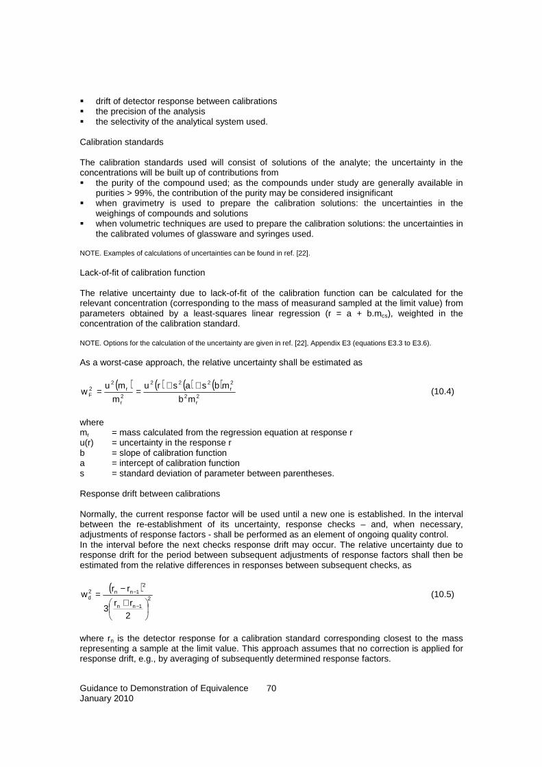
Guidance to Demonstration of Equivalence January 2010
70
� drift of detector response between calibrations � the precision of the analysis � the selectivity of the analytical system used. Calibration standards The calibration standards used will consist of solutions of the analyte; the uncertainty in the concentrations will be built up of contributions from � the purity of the compound used; as the compounds under study are generally available in
purities > 99%, the contribution of the purity may be considered insignificant � when gravimetry is used to prepare the calibration solutions: the uncertainties in the
weighings of compounds and solutions � when volumetric techniques are used to prepare the calibration solutions: the uncertainties in
the calibrated volumes of glassware and syringes used. NOTE. Examples of calculations of uncertainties can be found in ref. [22]. Lack-of-fit of calibration function The relative uncertainty due to lack-of-fit of the calibration function can be calculated for the relevant concentration (corresponding to the mass of measurand sampled at the limit value) from parameters obtained by a least-squares linear regression (r = a + b.mcs), weighted in the concentration of the calibration standard. NOTE. Options for the calculation of the uncertainty are given in ref. [22], Appendix E3 (equations E3.3 to E3.6). As a worst-case approach, the relative uncertainty shall be estimated as
( ) ( ) ( ) ( )22
2222
2
22
r
r
r
rF
mb
mbsasru
m
muw
++== (10.4)
where mr = mass calculated from the regression equation at response r u(r) = uncertainty in the response r b = slope of calibration function a = intercept of calibration function s = standard deviation of parameter between parentheses. Response drift between calibrations Normally, the current response factor will be used until a new one is established. In the interval between the re-establishment of its uncertainty, response checks – and, when necessary, adjustments of response factors - shall be performed as an element of ongoing quality control. In the interval before the next checks response drift may occur. The relative uncertainty due to response drift for the period between subsequent adjustments of response factors shall then be estimated from the relative differences in responses between subsequent checks, as
( )2
1nn
21nn2
d
2rr
3
rrw
+−=
−
− (10.5)
where rn is the detector response for a calibration standard corresponding closest to the mass representing a sample at the limit value. This approach assumes that no correction is applied for response drift, e.g., by averaging of subsequently determined response factors.

Guidance to Demonstration of Equivalence January 2010
71
Selectivity The analytical system used shall be optimized in order to minimize uncertainty due to the presence of potential interferents. Tests shall be performed with typical interferents at levels corresponding to 5 times the limit value of the compound under study. The uncertainty due to interferences may be obtained from ISO 14956 [24] as
( )2
0
202
R r3rr
w−= + (10.6)
where r+ represents the response with interferent, and r0 represents the response without. 10.3.2.1.5 Combined uncertainty in the sampled mass The contributions given above are combined to give the uncertainty of the mass of compound in the air sample as
( ) ( )2R
2d
2F
2anal2
cs
cs2
2sam
sam2
wwwwnm
mu
m
mu++++= (10.7)
where n = number of calibration standards used to construct the calibration function (≥5) wR = relative uncertainty due to (lack of) selectivity of the analytical system. 10.3.2.2 Mass of compound in sample blank The mass of compound in a sample blank is determined by analysis under repeatability conditions of a series of sample blanks; a minimum of 6 replicate analyses should be performed. The uncertainty is then calculated using the slope of the calibration function extrapolated to the blank response level as
( )bl
2bl
bl2
nbs
mu = (10.8)
where sbl = standard deviation of the replicate blank analyses n = number of replicate analyses bbl = slope of the calibration function at the blank response level. When the blank response is below 3 times the noise level of the detector, then the blank level and its uncertainty may be calculated from the detector noise level using the slope of the calibration function extrapolated to zero response assuming a uniform distribution as
0
0bl b2
r3m = (10.9)
( )12
r9mu
20
bl2 = (10.10)
where r0 = noise level b0 = slope of calibration function at zero response.

Guidance to Demonstration of Equivalence January 2010
72
10.3.2.3 Combined uncertainty The combined relative uncertainty of the compound mass in the air sampled is obtained by combination of contributions given in Clauses 10.3.2.1 – 10.3.2.2 as
( ) ( ) ( )( )2
blsam
bl2
sam2
2
2lab2
lab,CMmm
mumu
m
muw
-
+== (10.11)
10.2.3.4 Expanded uncertainty The expanded relative uncertainty of the candidate method resulting from the laboratory experiments, WCM,lab at the 95% confidence level is obtained by multiplying wCM,lab with a coverage factor appropriate to the number of degrees of freedom resulting from the performance of the test programme. This can be calculated by applying the Welch-Satterswaithe equation (ENV 13005, H2). For a large number of degrees of freedom, a coverage factor of 2 is used.
NOTE. As a first approximation, the number of degrees of freedom may be based on that of an uncertainty contribution covering more than 50% of the variance budget.
10.3.2.5 Evaluation of results of the laboratory tests The resulting WCM,lab is compared with the expanded relative uncertainty based on the data quality objective for the standard method Wdqo. If WCM,lab ≤ Wdqo, the field test programme can be performed; if not, the candidate method shall first be improved, and relevant changes tested in the laboratory test programme. 10.4 Field test programme 10.4.1 General When required, field tests shall be performed in which candidate and reference methods are compared side-by-side. The measurements will serve to assess � ‘between-sample’ uncertainty of the candidate method through the use of replicate samples � ‘comparability’ of the candidate and reference methods. For constituents of particulate matter, sampling is not a part of the equivalence testing. Therefore, sub-samples from high-volume samples with different loadings may be used to obtain the required information. In principle, 8 or more sub-samples may be obtained from one high-volume sample and the homogeneity of compound loadings on the sub-samples has been demonstrated for benzo[a]pyrene [29] to be better than < 4 % (coefficient of variation) when applying the reference method. In order to assure proper implementation of the reference method, a minimum of two samples shall be analyzed by application of the reference method. The number of replicate samples needed to determine the between-sampler uncertainty of the candidate method (reference method) will depend on whether the candidate method is to be used by more than one laboratory. When used by one laboratory, a minimum of six sub-samples will be analyzed using the candidate method. When used by more than one laboratory, the field test is also used to assess between-laboratory contributions to the uncertainty of the measurement results. For this purpose, each laboratory will analyze a minimum of two samples using the candidate method.

Guidance to Demonstration of Equivalence January 2010
73
10.4.2 Experimental conditions Samples shall be representative of typical conditions for which equivalence will be claimed, including possible episodes of high concentrations. A minimum of 4 comparisons shall be performed with particular emphasis on the following variables, if appropriate: � Composition of the air, notably high and low concentrations of the measured compound and
potential interferents � Air humidity and temperature (high and low) to cover any effects on extraction efficiency. For the candidate method a minimum of 20 different high-volume samples per comparison – to be divided into 8 sub-samples each - shall be collected. Alternatively, a minimum of 160 samples obtained using a low-volume reference sampler may be used. Samplers and instruments shall be positioned in such a way that the effect of spatial inhomogeneity of the compound concentration in the sampled air is negligible in comparison with other uncertainty contributions. Both methods shall be operated under conditions reflecting practical application in the field, e.g., calibration intervals, response checks, analysis of blank samples. During the tests, the following information shall be collected and recorded � Calibration procedures, equipment and intervals � (Results of) quality checks � Other conditions relevant for the analyses performed. 10.4.3 Evaluation of test results 10.4.3.1 Suitability of the dataset Of the full dataset, at least 20% of the results shall be greater than or equal to the upper assessment threshold specified in [2]. Data shall only be removed from the data set when sound technical reasons can be found for doing so. All valid data shall be used for further evaluation. NOTE. Indications of outlying data within replicate sets may be obtained using Grubb’s tests on the individual single-period variances. Tests are to be performed at the 99% level. 10.4.3.2 Calculation of performance characteristics 10.4.3.2.1 Between-sample uncertainty The relative between-sample uncertainty for individual laboratories wbs is calculated for the full dataset from the differences of results of the replicate analysis of the samples as:
( )2
2n
1i2,i1,i
2bs
yn2
yyw
∑=
−= for duplicate samples (10.12)
where yi,1 and yi,2 are the results of parallel measurements for a single period i
y = average of all measurement results of the candidate method

Guidance to Demonstration of Equivalence January 2010
74
n = number of measurement results.
( )( ) 2
n
1i
p
1j
2
ij,i2bs
y1pn
yy
w−
−=∑∑
= = for replicate samplers with p > 2 (10.13)
where yij = result of measurement j for a single period i
y i = mean result for period i p = number of replicates for period i. When more than one analytical laboratory is participating, equation 10.13 shall be used to calculate the between-laboratory uncertainty wbs. The wbs between-sample uncertainty component for each individual laboratory and the between-laboratory wbs (if relevant) shall comply with the criteria given in Annex A. If the performance of a single laboratory causes a method implemented by more than two laboratories to fail the criteria, then the results for this laboratory may be excluded, if sound technical grounds exist for doing so. 10.4.3.2.2 Comparison with reference method First, the performance of the reference method is checked by calculation of the relative between-sampler uncertainty as in eq. (10.12) or (10.13). The relative between-sample uncertainty for the reference method shall be ≤ 4%. For a comparison with the reference method first the results of replicate measurements are averaged to give data pairs ‘candidate method – reference method’ with equal measurement periods. For the evaluation of the uncertainty due to the ‘lack of comparability’ between candidate and reference method it is assumed that the relationship between measurement results of both methods can be described by a linear relation of the form:
ii bxay += (10.14) where xi is the average result of the reference method over period i. The relation between the average results of the candidate method and those of the reference method is established for the full dataset using a regression technique that leads to a symmetrical treatment of both variables. A commonly applied technique is orthogonal regression [29]. The uncertainty due to lack of comparability will be a function of the concentration of the measurand. The general relationship describing the dependence of uC-S on xi is given by
( ) ( ) ( ) ( )[ ]2ii2
i2CR x1baxu
2nRSS
yu −++−−
= (10.15)
where RSS = the sum of (relative) residuals resulting from the orthogonal regression

Guidance to Demonstration of Equivalence January 2010
75
u(xi) = random uncertainty of the results of the reference method. When more than one sample has been analyzed using the reference method, u(xi) may be calculated as ubs,RM/√p where ubs,RM is the reference between-sample uncertainty calculated using eq. (10.12) for 2 duplicates or eq. (10.13) for p replicates, using the reference results as input. Algorithms for the calculation of a and b and their variances are given in Annex C. RSS, the sum of (relative) residuals is calculated using eq. 10.16a or 10.16b, depending on whether the residuals or relative residuals are constant.
( )∑=
−−=n
1i
2ii bxayRSS when ( )2
ii bxay −− is constant (10.16a)
( )2
n
1i i
i2i 1
bxa
ybxaRSS ∑
=
−
++= when
2
i
i 1bxa
y
−
+is constant (10.16b)
10.4.3.3 Calculation of the combined uncertainty of candidate method The combined relative uncertainty of the candidate method wc,CM is calculated by combining the contributions found in 10.4.3.2.1 and 10.4.3.2.2 as follows:
( ) ( )2i
i2CR2
bsi2
CM,cy
yuwyw += (10.17)
In this way, wc,CM is expressed as a function of the compound concentration. The uncertainty at the limit value wCM is calculated by taking as yi the concentration at the limit value. 10.4.3.4 Calculation of the expanded uncertainty of candidate method The expanded relative uncertainty of the results of the candidate method is calculated by multiplying wc,CM by a coverage factor k reflecting the appropriate number of degrees of freedom resulting from the determination of wc,CM as
CM,cfield,CM wkW ⋅= (10.18)
In view of the large number of experimental results available, a coverage factor k=2 can be used. 10.4.4 Evaluation of results of field tests The resulting uncertainty estimate WCM,field is compared with the expanded relative uncertainty obtained from the laboratory test programme WCM,lab and the expanded relative uncertainty based on the data quality objective for the reference method Wdqo. In principle, three cases are possible 1. WCM,field ≤ WCM,lab: the candidate method is accepted as equivalent to the reference method 2. WCM,lab < WCM,field ≤ Wdqo : the candidate method is accepted conditionally; before final
acceptance, the uncertainty evaluation from the laboratory tests should be revisited and corrected such that situation 1 occurs
3. WCM,field > Wdqo: the candidate method is not accepted as equivalent method.

Guidance to Demonstration of Equivalence January 2010
76
11 REPORTING REQUIREMENTS Final reports on the Demonstration of Equivalence submitted to the National Competent Authority and further to the European Commission should contain – at minimum – the following information. Title of the method Executive summary General information 1. A summary of the principles of the candidate method; the full Standard Operating Procedure
of the method, including a description of ongoing QA/QC, shall be annexed. 2. The scope of equivalence testing, i.e., the differences between the candidate method and the
reference method that require specific tests to be performed. 3. A description of the conditions for which equivalence with the reference method is claimed,
e.g., concentration range, environmental conditions, type of location. 4. Sources of uncertainty data for unchanged parts of the EN standards enacting the reference
method, where relevant. 5. Names of the laboratories involved in the test programme(s) and the scope of their relevant
competences, e.g., EN-ISO 17025 accreditation. Laboratory test programme (where applicable) 6. The parameters tested in the laboratory programme. 7. A description of the test procedures used, including procedures for the establishment and
maintenance of measurement traceability where relevant, and procedures for quality control and quality assurance.
8. The test results, the results of the uncertainty assessment, and the results of their comparison with the relevant data quality objectives including uncertainty or, in the absence of data quality objectives, the results of the comparison between candidate method and reference method.
Field test programme (where applicable) 9. Full description of the test locations, test periods and conditions (e.g. temperature, humidity,
wind velocity, concentration level) 10. A description of the equipment and test procedures used, including procedures for the
establishment and maintenance of measurement traceability where relevant, and procedures for quality control and quality assurance.
11. The test results, the results of the uncertainty assessment, and the results of their comparison with the relevant data quality objectives including uncertainty, or, in the absence of data quality objectives, the results of the comparison between candidate method and reference method.
Conclusions 12. Results of the overall testing of the performance of the candidate method as compared to the
data quality objectives specified in the relevant EU Directive. 13. The overall conclusion about the equivalence including restrictions, if any, in the conditions
under which the claim to equivalence is valid or generalizations of the equivalence claim to other relevant conditions. Relevant conditions include concentration ranges, meteorological conditions, geographical locations and/or type(s) of monitoring sites.

Guidance to Demonstration of Equivalence January 2010
77
12 REFERENCES 1. Council Directive 2008/50/EC on ambient air quality and cleaner air for Europe. 2. Council Directive 2004/107/EC relating to arsenic, cadmium, mercury, nickel and polycyclic
aromatic hydrocarbons in ambient air. 3. EN 12341. Air quality – Determination of the PM10 fraction of suspended particulate matter –
reference method and field test procedure to demonstrate reference equivalence of measurement methods. CEN, Brussels, 1998.
4. EN 14211. Ambient air quality – Measurement method for the determination of the
concentration of nitrogen dioxide and nitrogen monoxide by chemiluminescence. CEN, Brussels, 2005.
5. EN 14212. Ambient air quality – Measurement method for the determination of the
concentration of sulphur dioxide by UV fluorescence. CEN, Brussels, 2005. 6. EN 14625. Ambient air quality – Measurement method for the determination of the
concentration of ozone by UV photometry. CEN, Brussels, 2005. 7. EN 14626. Ambient air quality – Measurement method for the determination of the
concentration of carbon monoxide by non-dispersive infrared spectrometry. CEN, Brussels, 2005.
8. EN 14662-1. Standard method for the determination of benzene in ambient air – Part 1:
Method with pumped sampling, thermal desorption and capillary gas chromatography. CEN, Brussels, 2005.
9. EN 14662-2. Standard method for the determination of benzene in ambient air – Part 2:
Method with pumped sampling, solvent desorption and capillary gas chromatography. CEN, Brussels, 2005.
10. EN 14662-3. Standard method for the determination of benzene in ambient air – Part 3:
Method with automated gas chromatographs. CEN, Brussels, 2005. 11. EN 14902. Ambient air quality – Standard method for the measurement of Pb, Cd, As and Ni
in the PM10 fraction of suspended particulate matter. CEN, Brussels, 2004. 12. EN 14907. Ambient Air Quality – Reference gravimetric measurement method for the
determination of the PM2.5 mass fraction of suspended particulate matter in ambient air. CEN, Brussels, 2005.
13. EN 15549. Ambient Air Quality – Standard method for the measurement of the concentration of benzo[a]pyrene in ambient air. CEN, Brussels, 2008.
14. EN 14662-4. Standard method for the determination of benzene in ambient air – Part 4: Method with difusive sampling, thermal desorption and capillary gas chromatography. CEN, Brussels, 2005.
15. EN 14662-5. Standard method for the determination of benzene in ambient air – Part 5:
Method with diffusive sampling, solvent desorption and capillary gas chromatography. CEN, Brussels, 2005.

Guidance to Demonstration of Equivalence January 2010
78
16. Gerboles, M.; Buzica, D.; Amanti, L. Modification of the Palmes diffusion tube and semi-empirical modelling of the uptake rate for monitoring nitrogen dioxide. Atmos. Environ., 39 (2005) 2579-2592.
17. Pfeffer, U.; Beier, R.; Zang, T. Measurements of nitrogen dioxide with diffusive samplers at traffic-related sites in North Rhine Westfalia. Gefahrstoffe – Reinhaltung der Luft, 66 (2006) 38-44.
18. ISO 6144. Gas analysis – Preparation of calibration gas mixtures – Static volumetric method. ISO, 2002.
19. ISO 6145. Gas analysis – Preparation of calibration gas mixtures using dynamic volumetric methods – all parts.
20. Eurachem / Citac Guide G4. Quantifying Uncertainty in Analytical Measurement, 2nd edition (2000).
21. Draft-VDI 2100, part 4. Gaseous ambient air measurement. Indoor air pollution measurement – Gas chromatographic determination of organic compounds – Calibration procedures as a measure for quality assurance. VDI, Düsseldorf, 2002.
22. EN-ISO 14956. Air quality – Evaluation of the suitability of a measurement method by comparison with a stated measurement uncertainty. ISO, Geneva, 2001.
23. EN 13528-1. Ambient air quality – Diffusive samplers for the determination of gases and vapours – Requirements and test methods – Part 1: General requirements.
24. EN 13528-2. Ambient air quality – Diffusive samplers for the determination of gases and vapours – Requirements and test methods – Part 2: Specific requirements and test methods.
25. EN 13528-3. Ambient air quality – Diffusive samplers for the determination of gases and vapours – Part 3: Guide to selection, use and maintenance.
26. Hafkenscheid, Th. L. Diffusive sampler validation using measurement uncertainty as performance characteristic. Proceedings of the International Conference Measuring Air Pollutants by Diffusive sampling. Montpellier, 2001. EUR 20242 EN, EC, 2002.
27. Massart, D.L.; A. Dijkstra, L. Kaufman. Evaluation and Optimization of Laboratory Methods and Analytical Procedures. Elsevier, Amsterdam, 1978.
28. Allegrini, I.; A. Febo, C. Perrino. Critical aspects of harmonization in particulate matter measurements: evaluation of methods and equivalence procedures. Paper presented at the International Conference on QA/QC in the field of emission and air quality measurements. Prague, 2003.
29. CEN TC 264 WG 21. Test protocol for field validation of B[a]P reference measurement methods. Working Group Document N67.
30. EUR Report 22341Field experiments to validate the CEN Standard measurement method for PM 2.5. JRC-IES, 2006.
31. Landesamt für Natur, Umwelt und Verbraucherschutz NRW. PM10-vergleichsmessungen der deutschen Bundesländer. Materialienband 66, 2005.

Guidance to Demonstration of Equivalence January 2010
79
ANNEX A Table A1. Criteria for between-sampler/instrument and between-laboratory uncertainties for specified compounds
Compound Required Standard
Uncertainty (%) *
Between-sampler/ instrument
(%)
Between lab
(%)
Sulphur dioxide 7,5 5 5 Nitrogen dioxide 7,5 5 5 Ozone 7,5 5 5 Carbon monoxide 7,5 5 5 Benzene 12,5 3 7,5 Benz[a]pyrene 25 4 15 Nickel 20 5 12,5 Cadmium 20 5 12,5 Lead 12,5 4 7,5 Arsenic 20 5 12,5 * 50% of the data-quality objective expanded uncertainty for continuous or fixed measurements as specified in Directives 2008/50/EC and 2004/107/EC.
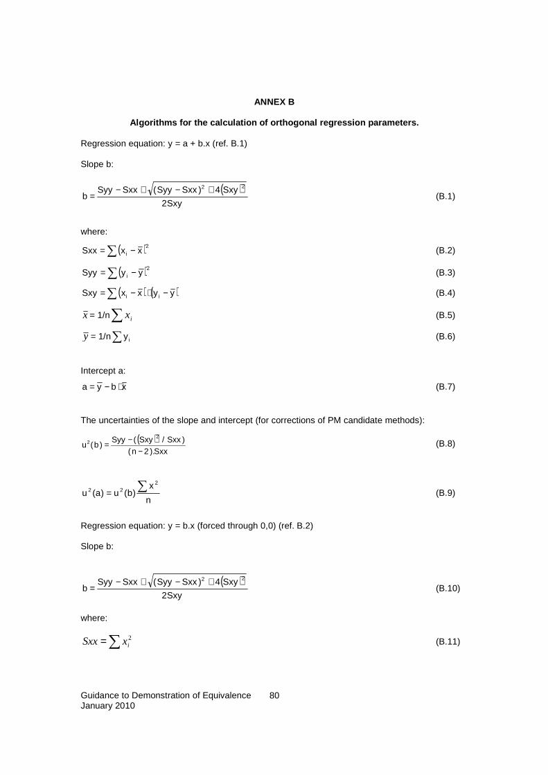
Guidance to Demonstration of Equivalence January 2010
80
ANNEX B
Algorithms for the calculation of orthogonal regres sion parameters. Regression equation: y = a + b.x (ref. B.1) Slope b:
( )Sxy2
Sxy4)SxxSyy(SxxSyyb
22 +−+−= (B.1)
where:
( )2i xxSxx ∑ −= (B.2)
( )2
i yySyy ∑ −= (B.3)
( ) ( )yyxxSxy ii −⋅−=∑ (B.4)
x = 1/n∑ ix (B.5)
y = 1/n∑ iy (B.6)
Intercept a:
xbya ⋅−= (B.7)
The uncertainties of the slope and intercept (for corrections of PM candidate methods):
( )Sxx).2n(
)Sxx/Sxy(Syy)b(u
22
−−= (B.8)
n
xbuau ∑=
222 )()( (B.9)
Regression equation: y = b.x (forced through 0,0) (ref. B.2) Slope b:
( )Sxy2
Sxy4)SxxSyy(SxxSyyb
22 +−+−= (B.10)
where:
∑= 2ixSxx (B.11)

Guidance to Demonstration of Equivalence January 2010
81
∑= 2iySyy (B.12)
∑= ii yxSxy (B.13)
Variance of the slope:
( )Sxx).1n(
)Sxx/Sxy(Syy)b(u
22
−−= (B.14)
References B.1 Kendall, M.G., Stuart, A. The Advanced Theory of Statistics. Griffin, London, 1969. B.2 Beijk, R.,D. Mooibroek, J. van de Kassteele, R. Hoogerbrugge. PM10: Equivalence study
2006. Demonstration of equivalence for the automatic PM10 measurements in the Dutch National Air Quality Monitoring Network. A technical background report. RIVM Report 680708002/2008.

Guidance to Demonstration of Equivalence January 2010
82
ANNEX C
Example of equivalence studies of PM samplers equip ped with filter changers Source: EN 14907 field experiments [30] Locations: Berlin, Madrid, Duisburg, Vienna, Rome, Vredepeel, Aspvreten, Teddington Manual sampler: Low-volume sampler LVS Automated sampler: LVS with sequential sampler SEQ REGRESSION OUTPUT slope b 1,001 uncertainty of b 0,005 intercept a -0,25 uncertainty of a 0,14 number of data pairs 576 EQUIVALENCE TEST RESULTS random term 1,82 µg/m³ bias at LV -0,21 µg/m³ combined uncertainty 1,83 µg/m³ relative uncertainty 6,1% pass ref sampler uncertainty 0,82 µg/m³ limit value 30 µg/m³
Example of equivalence studies of low- and high-vol ume PM samplers Sources: JRC-IES; LAI (DE); STIMES (DE); UBA-Austria Locations: Various Low-volume sampler LVS 2,3 m3 h-1 High-volume sampler HVS 30 m3 h-1
REGRESSION OUTPUT
slope b 0,986 uncertainty of b 0,004 sign intercept a -0,06 uncertainty of a 0,16 number of data pairs 790 EQUIVALENCE TEST RESULTS random term 2,4 µg/m³ bias at LV -0,8 µg/m³ combined uncertainty 2,5 µg/m³ relative uncertainty 5,0% pass ref sampler uncertainty 0,67 µg/m³ limit value 50 µg/m³

Guidance to Demonstration of Equivalence January 2010
83
ANNEX D
Requirements for quality control of candidate metho ds for PM D.1 Frequency of calibrations, checks and maintenance The checks and calibrations together with their frequency are summarised in Table D.1. Criteria are also given for readjustment, calibration or maintenance of the instruments.
Table D.1 — Required frequency of calibration, chec ks and maintenance.
Calibration, checks and maintenance Section Frequen cy Action criteria a
Checks of status values of operational parameters (see 7.5.3)
8.4.3 Daily See below
Checks of sensors for temperatures, pressure and/or humidity
8.4.4 Every 3 monthsb ± 2 °C ± 1 kPa
± 5% RH Calibration of sensors for temperatures, pressure and/or humidity
8.4.5 Every year ± 1 °C ± 0,2 kPa
± 2,5% RH Check of the CM flow rate(s) 8.4.6 Every 3 monthsb 4% Calibration of the CM flow rate(s) 8.4.7 Every year 3% Zero check of the CM reading 8.4.8 Every year 2 µg/m3 Calibration of the CM mass measuring systemc 8.4.9 As recommended by the
manufacturer and after repair, but at least every year
3%
Regular maintenance of components of the AMS
8.5 As required by manufacturer
a With reference to nominal values. b The frequency of the checks may be relaxed when sufficient history exists demonstrating that drifts of sensor readings and flow rates remain within the specified requirements. Calibrations shall be performed every year. c For optical CM this calibration can only be performed by comparison with the reference method or with a reference optical instrument. D.2 Checks of operational parameters During its operation the CM status signals of – at minimum – the following parameters shall be checked against the criteria given in Table D.1: � flow rate, and pressure drop over sample filter (if relevant) � sampling time and sample volume � mass concentration of relevant PM fraction(s) � ambient temperature � ambient pressure � air temperature in measuring section � temperature of the sampling inlet if a heated inlet is used.
Values of parameters for which Table D.1 gives no criteria shall be checked on the basis of plausibility of results.
In addition, the instrument status shall be checked for warning and alarm messages.
D.3 Checks of CM sensors Where temperature, pressure (difference) and/or relative humidity sensors are essential for controlling the proper functioning of the instrument, these shall be checked using appropriate transfer standards with readings traceable to (inter)nationally accepted standards. These checks must be performed before the flow rate check.
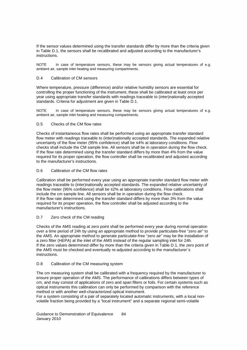
Guidance to Demonstration of Equivalence January 2010
84
If the sensor values determined using the transfer standards differ by more than the criteria given in Table D.1, the sensors shall be recalibrated and adjusted according to the manufacturer’s instructions. NOTE In case of temperature sensors, these may be sensors giving actual temperatures of e.g. ambient air, sample inlet heating and measuring compartments.
D.4 Calibration of CM sensors Where temperature, pressure (difference) and/or relative humidity sensors are essential for controlling the proper functioning of the instrument, these shall be calibrated at least once per year using appropriate transfer standards with readings traceable to (inter)nationally accepted standards. Criteria for adjustment are given in Table D.1. NOTE In case of temperature sensors, these may be sensors giving actual temperatures of e.g. ambient air, sample inlet heating and measuring compartments.
D.5 Checks of the CM flow rates Checks of instantaneous flow rates shall be performed using an appropriate transfer standard flow meter with readings traceable to (inter)nationally accepted standards. The expanded relative uncertainty of the flow meter (95% confidence) shall be ≤4% at laboratory conditions. Flow checks shall include the CM sample line. All sensors shall be in operation during the flow check. If the flow rate determined using the transfer standard differs by more than 4% from the value required for its proper operation, the flow controller shall be recalibrated and adjusted according to the manufacturer’s instructions. D.6 Calibration of the CM flow rates Calibration shall be performed every year using an appropriate transfer standard flow meter with readings traceable to (inter)nationally accepted standards. The expanded relative uncertainty of the flow meter (95% confidence) shall be ≤2% at laboratory conditions. Flow calibrations shall include the cm sample line. All sensors shall be in operation during the flow check. If the flow rate determined using the transfer standard differs by more than 3% from the value required for its proper operation, the flow controller shall be adjusted according to the manufacturer’s instructions. D.7 Zero check of the CM reading Checks of the AMS reading at zero point shall be performed every year during normal operation over a time period of 24h by using an appropriate method to provide particulate-free “zero air” to the AMS. An appropriate method to generate particulate-free “zero air” may be the installation of a zero filter (HEPA) at the inlet of the AMS instead of the regular sampling inlet for 24h. If the zero values determined differ by more than the criteria given in Table D.1, the zero point of the AMS must be checked and eventually re-adjusted according to the manufacturer´s instructions. D.8 Calibration of the CM measuring system The cm measuring system shall be calibrated with a frequency required by the manufacturer to ensure proper operation of the AMS. The performance of calibrations differs between types of cm, and may consist of applications of zero and span filters or foils. For certain systems such as optical instruments this calibration can only be performed by comparison with the reference method or with another well-characterized optical instrument. For a system consisting of a pair of separately located automatic instruments, with a local non-volatile fraction being provided by a “local instrument” and a separate regional semi-volatile

Guidance to Demonstration of Equivalence January 2010
85
fraction being provided by a “regional instrument”, whose results are combined to form the measurement result at the local site, a well-characterized specimen of a regional instrument may be used as a calibration instrument. D.9 Maintenance D.9.1 Change of consumables as applicable The life of all CM consumables should be determined at the initial installation. Site-specific maintenance periods should be devised for the replacement of such consumables. D.9.2 Regular maintenance of components of the AMS The manufacturer’s recommendations should be followed for the routine maintenance of the AMS. NOTE For highly polluted sites the frequency should be increased.

Guidance to Demonstration of Equivalence January 2010
86
ANNEX E
Members of the Equivalence Working Group (alphabeti cal order)
Pascual Perez Ballesta European Commission – Joint Research Centre – Institute of Environment and Sustainability
Antonio Febo Centro Nationale di Ricerca (Italy) Rosalia Fernandez-Patier Instituto Sanitad Carlos III (Spain) Marina Fröhlich Umweltbundesamt (Austria) Saul dos Santos Garcia Instituto Sanitad Carlos III (Spain) Theo Hafkenscheid (chairman) Nederlands Meetinstituut (Netherlands) Stefan Jacobi European Commission – Directorate-General Environment Ton van der Meulen Rijksinstituut voor Volksgezondheid en Milieu (Netherlands) Don Munns CEN Technical Committee 264 ‘Air Quality’ Hans-Ulrich Pfeffer LANUV Nordrhein-Westfalen (Germany) Jean Poulleau INERIS (France) Kevin Saunders KERIS Ltd. (United Kingdom) Jari Walden Finnish Meteorological Institute (Finland) Peter Woods National Physical Laboratory (United Kingdom)

Guidance to Demonstration of Equivalence January 2010
87
ANNEX F
Examples of results of equivalence testing for AMS for particulate matter
Introduction This annex contains some examples of results of equivalence testing for automated methods for measurement of PM2.5, and PM10, performed using the algorithms given in Clause 9.5-9.7. The measurement data used for PM2.5 were taken from the validation study carried out by CEN TC 264 WG 15. This annex gives three examples: � One in which the CM for one location does not fulfil the requirements for equivalence � One in which the CM for one location does not fulfil the requirements until after correction � One in which no correction of results is needed for one location to lead to acceptance of the
CM as an equivalent method. The measurement data used for PM10 were supplied by the Landesamt für Natur, Umwelt und Verbraucherschutz Nordrhein-Westfalen – LANUV (Germany). Using the algorithms presented in Clause 9.5 it is relatively easy to judge whether corrections may lead to an improvement beyond meeting the equivalence requirements: unless the slope b of the regression equation obtained for uncorrected results is high, a random uncertainty above 12,5% of the limit value concentration (about 2,5 µg.m-3 for PM2.5 ; about 6,3 µg.m-3 for PM10) is an indication that corrections will generally fail to bring the required improvement because of excessive scatter of the results of the reference and candidate methods when compared using regression, unless the slope of the regression equation is considerably higher than 1. It should be noted that for PM2.5 the between-sampler uncertainty for the reference method has been calculated from the data actually available from the validation study. For PM10 an uncertainty for the reference method of 1,5 µg.m-3 has been assumed, based on information supplied by LANUV.

Guidance to Demonstration of Equivalence January 2010
88
Examples of results – PM 2.5
Comparison of CM1 and RM – location A Full dataset (µg.m-3, uncorrected) RM1 RM2 CM1 RM1 RM2 CM1 RM1 RM2 CM1 RM1 RM2 CM1 23,8 25,8 24,5 63,8 66,2 51,5 10,5 10,4 7,3 71,1 71,5 55,8 21,5 20,5 21,8 56,4 57,7 41,3 6,8 7,3 6,8 55,4 55,1 38,1 25,4 23,5 23,0 48,2 49,7 41,3 7,1 7,3 10,6 49,4 49,2 38,6 14,1 13,5 12,9 58,0 59,7 52,0 14,7 16,1 15,9 51,8 51,6 40,2 15,2 15,2 14,0 44,0 44,5 38,0 39,2 39,3 32,6 55,7 55,1 43,0 21,2 20,4 20,5 29,7 30,3 23,1 45,8 46,2 36,0 19,6 18,6 15,1 31,0 31,2 26,8 26,9 24,3 33,1 33,2 24,4 58,7 58,7 46,6 29,8 27,5 25,6 24,8 24,4 28,7 14,2 14,4 10,0 50,2 50,9 38,8 38,0 37,1 35,1 4,5 6,8 8,6 34,3 33,6 29,8 6,3 6,2 8,4 16,4 17,2 17,5 19,3 19,6 19,9 51,7 51,0 47,8 18,1 16,0 19,9 25,1 24,0 24,6 41,4 42,6 35,2 44,0 43,6 42,7 41,9 45,6 44,3 33,1 32,2 29,3 42,4 43,0 37,7 39,9 40,8 37,3 37,2 37,0 35,8 43,4 48,2 37,3 27,4 28,1 19,9 46,8 47,2 42,0 71,4 73,2 67,0 42,6 46,2 36,1 28,8 29,0 22,9 33,5 33,6 28,2 68,6 64,9 55,9 45,2 44,3 40,2 12,3 12,7 11,0 43,4 41,9 36,5 69,6 67,5 57,5 40,4 41,6 22,4 10,6 10,9 12,1 37,1 38,3 31,9 25,5 26,1 20,5 31,9 31,0 21,3 12,3 14,3 65,7 66,5 57,4 6,3 4,6 7,1 37,7 36,6 35,5 26,8 26,5 25,6 57,7 57,2 43,6 12,7 11,6 11,7 47,9 45,2 38,6 40,2 40,6 33,1 32,8 33,9 21,2 13,8 13,3 13,6 71,6 68,7 53,4 15,7 15,9 13,7 22,6 24,0 22,5 25,9 26,5 23,4 54,2 53,4 53,9 17,1 16,8 16,4 58,1 58,3 52,0 39,7 39,3 25,3 61,4 58,7 56,1 37,2 36,9 32,4 63,9 63,0 55,1 10,9 10,4 4,2 69,5 68,6 57,7 29,9 30,6 23,5 45,6 46,3 39,3 15,7 14,9 11,7 85,2 85,0 75,4 40,4 42,7 33,3 23,9 25,6 19,5 10,1 9,7 11,8 59,0 61,8 50,3 52,6 52,4 43,9 30,8 30,9 21,9 12,2 12,6 11,6 59,8 60,5 48,9 22,8 23,0 16,3 37,4 36,6 27,2 17,4 16,9 16,0 9,0 9,9 12,9 29,7 28,3 18,5 37,1 36,9 29,3 8,8 7,8 8,8
10,0 11,0 13,9 22,0 22,4 10,5 44,3 43,1 36,2 19,7 19,2 19,0 Evaluation of uncorrected data for CM1 RESULTS OF REGRESSION EQUIVALENCE TEST RESULTS slope b 0,819* random term 3,6 µg/m³ uncertainty of b 0,019 bias at LV -4,3 µg/m³ intercept a 1,11 combined uncertainty 5,6 µg/m³ uncertainty of a 0,74 relative uncertainty 18,6% fail number of data pairs 111 RM uncertainty 0,9 µg/m³ limit value 30 µg/m³ * Significant at 95% confidence level. Evaluation of data for CM1 after correction for slope RESULTS OF REGRESSION EQUIVALENCE TEST RESULTS slope b 1,006 random term 4,4 µg/m³ uncertainty of b 0,023 bias at LV 1,3 µg/m³ intercept a 1,15 combined uncertainty 4,6 µg/m³ uncertainty of a 0,90 relative uncertainty 15,4% fail number of data pairs 111 RM uncertainty 0,9 µg/m³ limit value 30 µg/m³
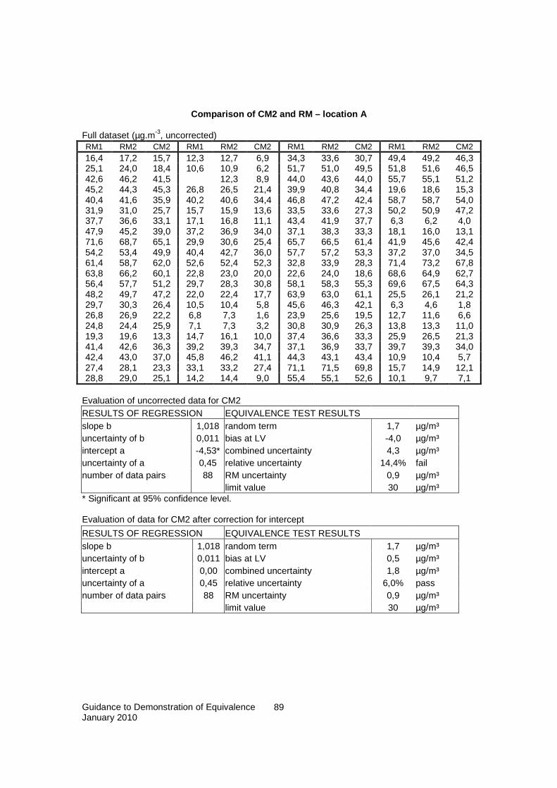
Guidance to Demonstration of Equivalence January 2010
89
Comparison of CM2 and RM – location A
Full dataset (µg.m-3, uncorrected) RM1 RM2 CM2 RM1 RM2 CM2 RM1 RM2 CM2 RM1 RM2 CM2 16,4 17,2 15,7 12,3 12,7 6,9 34,3 33,6 30,7 49,4 49,2 46,3 25,1 24,0 18,4 10,6 10,9 6,2 51,7 51,0 49,5 51,8 51,6 46,5 42,6 46,2 41,5 12,3 8,9 44,0 43,6 44,0 55,7 55,1 51,2 45,2 44,3 45,3 26,8 26,5 21,4 39,9 40,8 34,4 19,6 18,6 15,3 40,4 41,6 35,9 40,2 40,6 34,4 46,8 47,2 42,4 58,7 58,7 54,0 31,9 31,0 25,7 15,7 15,9 13,6 33,5 33,6 27,3 50,2 50,9 47,2 37,7 36,6 33,1 17,1 16,8 11,1 43,4 41,9 37,7 6,3 6,2 4,0 47,9 45,2 39,0 37,2 36,9 34,0 37,1 38,3 33,3 18,1 16,0 13,1 71,6 68,7 65,1 29,9 30,6 25,4 65,7 66,5 61,4 41,9 45,6 42,4 54,2 53,4 49,9 40,4 42,7 36,0 57,7 57,2 53,3 37,2 37,0 34,5 61,4 58,7 62,0 52,6 52,4 52,3 32,8 33,9 28,3 71,4 73,2 67,8 63,8 66,2 60,1 22,8 23,0 20,0 22,6 24,0 18,6 68,6 64,9 62,7 56,4 57,7 51,2 29,7 28,3 30,8 58,1 58,3 55,3 69,6 67,5 64,3 48,2 49,7 47,2 22,0 22,4 17,7 63,9 63,0 61,1 25,5 26,1 21,2 29,7 30,3 26,4 10,5 10,4 5,8 45,6 46,3 42,1 6,3 4,6 1,8 26,8 26,9 22,2 6,8 7,3 1,6 23,9 25,6 19,5 12,7 11,6 6,6 24,8 24,4 25,9 7,1 7,3 3,2 30,8 30,9 26,3 13,8 13,3 11,0 19,3 19,6 13,3 14,7 16,1 10,0 37,4 36,6 33,3 25,9 26,5 21,3 41,4 42,6 36,3 39,2 39,3 34,7 37,1 36,9 33,7 39,7 39,3 34,0 42,4 43,0 37,0 45,8 46,2 41,1 44,3 43,1 43,4 10,9 10,4 5,7 27,4 28,1 23,3 33,1 33,2 27,4 71,1 71,5 69,8 15,7 14,9 12,1 28,8 29,0 25,1 14,2 14,4 9,0 55,4 55,1 52,6 10,1 9,7 7,1
Evaluation of uncorrected data for CM2 RESULTS OF REGRESSION EQUIVALENCE TEST RESULTS slope b 1,018 random term 1,7 µg/m³ uncertainty of b 0,011 bias at LV -4,0 µg/m³ intercept a -4,53* combined uncertainty 4,3 µg/m³ uncertainty of a 0,45 relative uncertainty 14,4% fail number of data pairs 88 RM uncertainty 0,9 µg/m³ limit value 30 µg/m³ * Significant at 95% confidence level. Evaluation of data for CM2 after correction for intercept
RESULTS OF REGRESSION EQUIVALENCE TEST RESULTS slope b 1,018 random term 1,7 µg/m³ uncertainty of b 0,011 bias at LV 0,5 µg/m³ intercept a 0,00 combined uncertainty 1,8 µg/m³ uncertainty of a 0,45 relative uncertainty 6,0% pass number of data pairs 88 RM uncertainty 0,9 µg/m³ limit value 30 µg/m³

Guidance to Demonstration of Equivalence January 2010
90
Comparison of CM2 and RM – location B
Full dataset (µg.m-3, uncorrected) RM1 RM2 CM2 RM1 RM2 CM2 RM1 RM2 CM2 RM1 RM2 CM2 22,5 20,3 21,6 12,8 13,4 14,8 19,0 19,6 21,3 30,5 25,7 29,4 30,7 28,5 28,2 13,5 12,8 10,2 17,3 17,3 13,9 19,6 15,1 15,7 16,1 17,7 13,0 11,7 11,7 13,3 9,6 10,3 7,8 39,0 43,7 38,6 12,4 13,7 13,0 12,5 12,0 14,4 28,3 29,5 33,0 18,2 19,3 25,7 13,8 13,7 12,8 11,4 10,8 12,2 10,8 10,6 8,1 10,9 10,7 13,0 9,5 9,8 10,2 11,7 11,9 13,5 14,5 15,4 14,5 10,4 11,3 10,0
16,9 19,5 15,9 29,7 29,6 31,8 31,3 31,2 29,7 13,8 14,6 14,8 20,2 21,6 19,0 18,5 18,6 20,6 26,8 27,2 27,1 10,5 10,3 12,7 21,3 24,6 18,7 24,5 24,3 27,6 19,1 19,4 20,3 20,2 22,4 22,0 30,8 34,8 26,5 40,8 40,8 39,0 14,3 15,3 13,8 32,2 33,4 26,7 49,7 55,7 49,8 10,8 10,8 13,6 18,8 21,0 22,1 13,5 13,6 13,9 11,8 13,5 12,3 10,5 11,9 11,7 15,2 20,2 17,8 13,5 12,9 12,6 11,6 12,6 10,9 8,0 8,8 11,9 43,9 39,9 34,0 15,5 13,3 12,6 21,3 28,1 24,2 23,3 23,3 22,9 18,3 16,4 13,6 17,1 14,0 17,7 29,8 33,3 25,4 31,6 31,8 34,7 14,9 15,4 10,9 17,9 18,5 21,2 25,8 22,0 19,3 18,6 23,1 25,3 21,7 25,0
Evaluation of uncorrected data for CM1 RESULTS OF REGRESSION EQUIVALENCE TEST RESULTS slope b 0,934 random term 2,6 µg/m³ uncertainty of b 0,036 bias at LV -1,0 µg/m³ intercept a 0,977 combined uncertainty 2,7 µg/m³ uncertainty of a 0,794 relative uncertainty 9,2% pass number of data pairs 63 RM uncertainty 0,8 µg/m³ limit value 30 µg/m³

Guidance to Demonstration of Equivalence January 2010
91
Examples of results – PM 10
Comparison of CM1 and RM – location C Full dataset (µg.m-3, uncorrected)
RM CM1 RM CM1 RM CM1 RM CM1 RM CM1 RM CM1 36,0 35,9 81,2 58,6 22,0 14,7 24,9 23,0 45,5 32,4 24,0 21,8 13,9 15,0 41,8 24,9 21,5 16,7 25,8 21,3 20,9 17,5 39,4 32,0 33,3 24,6 52,5 34,2 19,4 18,2 27,2 25,4 49,5 38,1 50,4 36,7 44,8 31,0 29,7 13,7 21,5 20,3 15,3 13,3 46,2 39,6 22,8 16,9 53,6 43,5 17,4 9,2 25,7 23,1 26,4 22,0 26,6 26,7 30,9 20,9 47,9 30,0 30,2 20,3 30,3 29,5 21,9 19,0 34,0 29,3 24,6 21,5 33,9 19,0 35,5 21,6 24,8 22,3 36,9 35,8 23,3 19,2 33,5 28,1 23,6 14,5 36,8 23,0 26,9 27,9 31,6 24,5 25,3 20,5 33,8 30,6 29,2 18,5 39,3 25,4 29,9 27,1 41,1 30,8 36,0 29,6 34,6 31,5 19,0 11,2 40,9 35,0 27,7 25,1 46,7 40,0 27,5 16,1 38,5 27,4 14,3 11,9 23,8 20,8 15,8 11,4 57,0 53,3 15,8 14,2 37,3 19,6 37,8 27,7 31,2 30,4 26,5 22,5 55,1 52,4 15,9 16,2 66,0 60,8 23,8 21,8 50,2 38,5 21,4 17,0 25,2 21,5 23,5 22,0 38,4 31,5 19,6 15,0 44,1 38,3 18,4 12,9 21,8 22,3 17,4 16,1 23,9 18,3 62,5 49,7 24,0 17,1 29,4 27,0 29,6 22,2 33,8 27,2 46,9 41,4 66,2 52,1 22,4 18,4 19,2 8,6 44,7 39,1 30,4 23,4 39,9 31,1 42,6 31,4 20,5 18,9 31,3 22,5 25,0 22,7 57,6 43,3 8,2 7,7 40,0 29,1 18,0 15,8 34,0 24,0 22,4 19,3 37,0 29,4 22,0 21,7 44,2 38,5 16,2 14,4 26,0 19,4 26,1 20,1 39,6 33,0 41,8 34,8 50,4 42,5 29,2 23,1 33,6 28,0 30,3 18,9 25,5 20,2 38,2 33,6 44,5 34,3 40,8 30,2 51,8 42,7 13,9 12,0 39,8 29,8 14,4 13,7 23,4 16,9 39,9 22,5 22,6 16,9 23,5 21,2 28,2 20,6 27,7 20,4 29,5 25,6 20,8 15,2 27,7 22,2 22,9 20,3 16,5 14,9 18,4 14,3 59,6 44,5 18,3 15,6 21,4 17,3 24,1 24,3 15,3 16,2 11,1 10,4 39,0 21,7 18,7 16,5 31,1 29,4 39,6 27,2 30,5 28,4 23,4 20,7 45,1 25,2 12,2 8,9 24,0 20,8 29,0 18,6 32,0 26,6 43,8 34,2 21,5 16,4
Evaluation of uncorrected data for CM1 RESULTS OF REGRESSION EQUIVALENCE TEST RESULTS slope b 0,793* random term 3,5 µg/m³ uncertainty of b 0,024 bias at LV -10,3 µg/m³ intercept a 0,09 combined uncertainty 10,8 µg/m³ uncertainty of a 0,81 relative uncertainty 21,7% fail number of data pairs 157 RM between-sampler uncertainty 1,50 µg/m³ * Significant at 95% confidence level, Evaluation of data for CM1 after correction for slope
RESULTS OF REGRESSION EQUIVALENCE TEST RESULTS slope b 1,018 random term 4,7 µg/m³ uncertainty of b 0,030 bias at LV 0,44 µg/m³ intercept a -0,44 combined uncertainty 4,8 µg/m³ uncertainty of a 1,03 relative uncertainty 9,5% pass number of data pairs 157 RM between-sampler uncertainty 1,50 µg/m³

Guidance to Demonstration of Equivalence January 2010
92
Comparison of CM2 and RM – location C Full dataset (µg.m-3, uncorrected)
RM CM2 RM CM2 RM CM2 RM CM2 RM CM2 RM CM2 10,0 9,8 44,3 36,8 22,1 21,9 35,3 33,6 23,7 23,9 48,1 42,9 21,8 17,0 37,0 35,7 12,1 12,2 20,6 17,7 34,1 23,5 47,6 33,2 31,2 22,4 98,4 79,9 18,4 18,0 24,7 23,8 20,6 19,6 18,8 17,0 35,0 26,9 78,5 58,1 17,7 19,3 24,0 22,4 34,5 26,9 33,2 19,1 66,9 51,7 67,8 55,2 20,1 21,4 29,0 27,6 17,9 20,8 19,7 16,4 72,1 52,7 28,3 25,3 19,1 18,8 20,0 18,9 49,2 41,4 31,3 25,5 35,0 26,2 13,6 11,8 23,4 24,0 24,2 21,5 57,2 54,8 27,1 27,7 38,7 29,5 34,6 28,5 29,7 26,2 19,2 19,7 45,8 44,3 32,9 28,3 29,6 23,4 28,3 24,0 34,9 32,6 37,8 36,5 44,0 39,2 38,9 26,3 10,7 10,2 30,8 27,9 20,1 16,0 23,7 22,9 14,5 13,7 31,1 21,3 10,8 9,5 36,7 28,7 27,0 25,2 30,9 29,5 21,5 21,8 21,6 18,2 30,7 27,4 52,0 45,0 28,5 25,6 46,8 44,2 21,2 20,9 75,0 60,4 43,3 32,7 43,0 37,3 25,1 22,1 54,9 53,7 18,9 16,1 35,4 28,8 13,8 14,0 44,5 41,8 49,1 36,5 62,4 59,1 26,7 21,5 21,5 16,1 26,2 20,6 28,7 27,3 24,2 17,9 47,7 47,9 42,6 33,3 96,4 81,2 16,0 15,6 38,1 34,2 29,7 26,6 19,8 18,5 58,2 43,9 40,3 31,4 63,8 53,6 56,4 55,8 26,8 24,3 20,9 21,2 33,0 25,2 7,2 6,9 45,0 40,8 22,8 21,0 24,5 22,2 27,4 24,2 39,0 30,5 13,4 13,8 38,7 32,9 16,6 13,5 51,4 41,0 44,9 39,6 21,1 15,3 54,4 45,5 56,7 50,9 25,6 24,9 41,7 35,3 27,8 22,3 82,9 69,8 37,0 28,3 61,1 53,4 13,9 12,5 18,3 17,1 24,6 19,2 22,8 15,8 15,8 16,5 58,0 51,9 16,4 14,6 18,9 16,6 20,7 17,0 17,7 11,9 23,4 18,6 85,4 75,0 22,0 17,5 20,5 12,4 24,3 17,2 12,2 12,6 16,3 12,6 18,3 16,8 37,9 29,0 48,1 42,6 15,3 12,0 43,7 38,3 9,3 8,9 37,0 30,0 47,7 36,4 17,0 14,1 15,5 14,3 35,5 24,8 18,1 17,1 79,1 66,2 21,8 18,3 21,1 18,9 27,5 26,8 29,8 23,4 51,0 41,6 52,8 46,0 15,0 13,9 23,6 19,4
Evaluation of uncorrected data for CM2 RESULTS OF REGRESSION EQUIVALENCE TEST RESULTS slope b 0,829* random term 2,7 µg/m³ uncertainty of b 0,014 bias at LV -7,7 µg/m³ intercept a 0,88 combined uncertainty 8,13 µg/m³ uncertainty of a 0,52 relative uncertainty 16,3% fail number of data pairs 159 RM between-sampler uncertainty 1,50 µg/m³ * Significant at 95% confidence level, Evaluation of data for CM2 after correction for slope
RESULTS OF REGRESSION EQUIVALENCE TEST RESULTS slope b 1,004 random term 3,5 µg/m³ uncertainty of b 0,017 bias at LV 1,1 µg/m³ intercept a 0,93 combined uncertainty 3,7 µg/m³ uncertainty of a 0,63 relative uncertainty 7,3% pass number of data pairs 159 RM between-sampler uncertainty 1,50 µg/m³