guidebook on dta data needs and interface options...

0-6657-P1

GUIDEBOOK ON DTA DATA NEEDS AND INTERFACE

OPTIONS FOR INTEGRATION INTO THE PLANNING

PROCESS Jennifer Duthie, PhD Natalia Ruiz Juri, PhD Christopher L. Melson C. Matt Pool Steve Boyles, PhD TxDOT Project 0-6657: Investigating Regional Dynamic Traffic Assignment Modeling for

Improved Bottleneck Analysis

AUGUST 2012, PUBLISHED DATE NOVEMBER 2012 Performing Organization: Center for Transportation Research The University of Texas at Austin 1616 Guadalupe, Suite 4.202 Austin, Texas 78701

Sponsoring Organization: Texas Department of Transportation Research and Technology Implementation Office P.O. Box 5080 Austin, Texas 78763-5080

Performed in cooperation with the Texas Department of Transportation and the Federal Highway Administration.

ii

Center for Transportation Research The University of Texas at Austin 1616 Guadalupe St, Suite 4.202 Austin, TX 78701 www.utexas.edu/research/ctr Copyright (c) 2012 Center for Transportation Research The University of Texas at Austin All rights reserved Printed in the United States of America

Disclaimers Author's Disclaimer: The contents of this report reflect the views of the authors, who

are responsible for the facts and the accuracy of the data presented herein. The contents do not necessarily reflect the official view or policies of the Federal Highway Administration or the Texas Department of Transportation (TxDOT). This report does not constitute a standard, specification, or regulation.

Patent Disclaimer: There was no invention or discovery conceived or first actually reduced to practice in the course of or under this contract, including any art, method, process, machine manufacture, design or composition of matter, or any new useful improvement thereof, or any variety of plant, which is or may be patentable under the patent laws of the United States of America or any foreign country.

Engineering Disclaimer NOT INTENDED FOR CONSTRUCTION, BIDDING, OR PERMIT PURPOSES.

Principle Investigator: Jennifer Duthie P. E. Designation: Research Supervisor

1

Section 1: Introduction

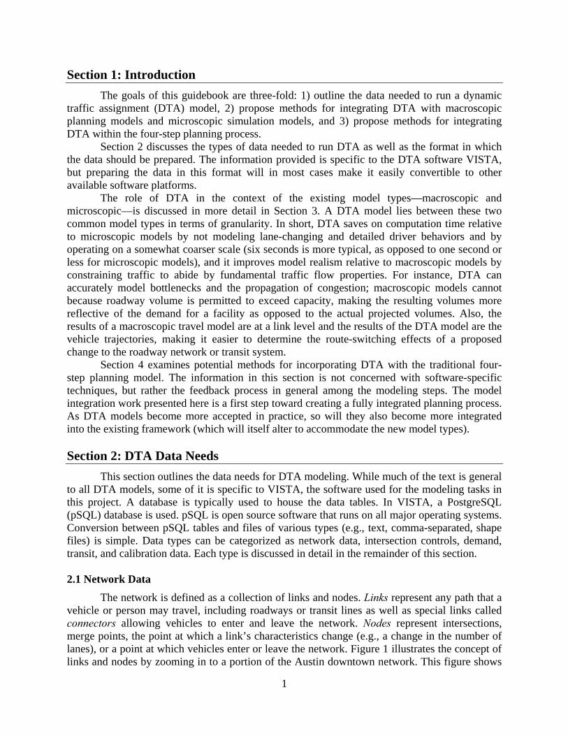
The goals of this guidebook are three-fold: 1) outline the data needed to run a dynamic traffic assignment (DTA) model, 2) propose methods for integrating DTA with macroscopic planning models and microscopic simulation models, and 3) propose methods for integrating DTA within the four-step planning process.

Section 2 discusses the types of data needed to run DTA as well as the format in which the data should be prepared. The information provided is specific to the DTA software VISTA, but preparing the data in this format will in most cases make it easily convertible to other available software platforms.

The role of DTA in the context of the existing model types—macroscopic and microscopic—is discussed in more detail in Section 3. A DTA model lies between these two common model types in terms of granularity. In short, DTA saves on computation time relative to microscopic models by not modeling lane-changing and detailed driver behaviors and by operating on a somewhat coarser scale (six seconds is more typical, as opposed to one second or less for microscopic models), and it improves model realism relative to macroscopic models by constraining traffic to abide by fundamental traffic flow properties. For instance, DTA can accurately model bottlenecks and the propagation of congestion; macroscopic models cannot because roadway volume is permitted to exceed capacity, making the resulting volumes more reflective of the demand for a facility as opposed to the actual projected volumes. Also, the results of a macroscopic travel model are at a link level and the results of the DTA model are the vehicle trajectories, making it easier to determine the route-switching effects of a proposed change to the roadway network or transit system.

Section 4 examines potential methods for incorporating DTA with the traditional four-step planning model. The information in this section is not concerned with software-specific techniques, but rather the feedback process in general among the modeling steps. The model integration work presented here is a first step toward creating a fully integrated planning process. As DTA models become more accepted in practice, so will they also become more integrated into the existing framework (which will itself alter to accommodate the new model types). Section 2: DTA Data Needs

This section outlines the data needs for DTA modeling. While much of the text is general to all DTA models, some of it is specific to VISTA, the software used for the modeling tasks in this project. A database is typically used to house the data tables. In VISTA, a PostgreSQL (pSQL) database is used. pSQL is open source software that runs on all major operating systems. Conversion between pSQL tables and files of various types (e.g., text, comma-separated, shape files) is simple. Data types can be categorized as network data, intersection controls, demand, transit, and calibration data. Each type is discussed in detail in the remainder of this section. 2.1 Network Data

The network is defined as a collection of links and nodes. Links represent any path that a vehicle or person may travel, including roadways or transit lines as well as special links called connectors allowing vehicles to enter and leave the network. Nodes represent intersections, merge points, the point at which a link’s characteristics change (e.g., a change in the number of lanes), or a point at which vehicles enter or leave the network. Figure 1 illustrates the concept of links and nodes by zooming in to a portion of the Austin downtown network. This figure shows

2

the nodes at intersections as well as two mid-block nodes, which in this case represent points where vehicles can enter and leave the network.

Figure 1. Links and nodes

Creating a network in DTA requires data on the geometry and characteristics of the links. Unlike some macroscopic modeling software, VISTA considers each direction of a roadway to be a separate link. The specific data types and formats are shown in Tables 1 and 2. Under “Type” for these two tables is the term centroid connector, which is a link that loads vehicles from an origin onto the network or from the network to a destination. All non-centroid connectors are listed as type mesoscopic (this is the type of simulation used by DTA software). DTA software’s basic network data needs are very similar to those needed by macroscopic modeling software.

Table 1. Link Geometry Data and Format

Data Type Format Description

ID Integer Unique identifier per link

Points Path Sequence of coordinate points that define the geometry of the link’s centerline (e.g., ‘[(-97.7388,30.2788),(97.739,30.2783)]’)

3

Table 2. Link Characteristic Data and Format



Type Integer 1 for mesoscopic simulation or 100 for centroid connectors

Source Integer Origin node ID of the link

Destination Integer Destination node ID of the link

Lanes Integer Number of lanes on the link

Length Numeric Length of the link in feet

Speed Numeric Speed limit of the link in miles per minute

Capacity Numeric Capacity of the link in vehicles per hour per lane

Optionally, users can model the links’ turning and merging bays. The information needed to do so is listed in Table 3.

Table 3. Link Bays Data and Format



Isleft Binary True if bay is to the left of the link; false if on the right

Isturn Binary True if bay is a turning bay; false if a merging bay

Lanes Integer Number of lanes in this bay

Length Numeric Length of the bay in feet

The basic information needed for each node is presented in Table 4. Under “Type” for this table is the term centroid, which here refers to a node that acts as an origin or destination for vehicles. All non-centroids are listed as type mesoscopic. Unlike some macroscopic modeling software, VISTA considers origins and destinations as separate nodes, even if they are located in the same place in the network.

Table 4. Node Data and Format


ID Integer Unique identifier per node

Type Integer 1 for mesoscopic simulation or 100 for centroid

X Numeric Horizontal position of the node (e.g., -97.7388)

Y Numeric Vertical position of the node (e.g., 30.2788) 2.2 Intersection Controls

Unlike macroscopic modeling, DTA has the capability to explicitly simulate intersection controls. If intersections are to be modeled, then information is needed on the location of the

4

controls and the timing plans. Each control is assumed to be associated with a node as shown in Table 4. Table 5 shows the basic information needed for each signal and Table 6 shows the information needed for each phase. Each node can have several phases associated with it and they will be processed in the order given in the “Phase” column. Unless specified otherwise, the simulation will begin with the green time for the first phase listed for each node with a signal. The “Linkfrom” and “Linkto” columns define each movement allowed during each phase. The arrays in these columns should be of equal length for each phase. So the first entry in each array specifies one allowed turning movement, the second entry in each array specifies another allowed turning movement, etc. For example, if a phase consists of vehicles approaching the intersection from link 4617 being allowed to make three turning movements (left to link 18305, right to link 118306, and through to link 18307), then the Linkfrom column will look like ‘{4617,4617,4617}’ and the Linkto column will look like ‘{18305,118306,18307}’.

Table 5. Signals Data and Format


ID Integer Unique identifier per control

Type Integer A constant 448

Timeoffset Integer Time in seconds to offset the beginning of the first phases from the beginning of simulation

Table 6. Signal Phases Data and Format


ID Integer Unique identifier per phase

Type Integer Either 1 (pretimed phase) or 2 (actuated phase)

Nodeid Integer ID of the corresponding node

Phase Integer Order of this phase in the timing plan

Timered Integer Red time for the phase

Timeyellow Integer Yellow time for the phase

Timegreen Integer Maximum green time for the phase

Linkfrom Array An array of approach link IDs

Linkto Array An array of departure link IDs

Stop signs and yield signs are currently implemented in VISTA by importing a list of nodes (in integer format) that contain each control type and then post-processing the network data to account for the effect of the control.

2.3 Demand

Simulation-based DTA models load vehicles onto the network throughout the simulation period. The typical process for achieving a dynamic demand table is to input a demand table from a macroscopic model that has the total number of vehicles desiring to travel between each

5

origin and destination during the entire time period of interest. A demand profile is then used to apportion this demand into the more fine-grained loading periods used by DTA (e.g., 10 minutes) and then the software internally uses a random number generator to assign actual departure times. Table 7 shows the data needed to input demand from a static planning model and Table 8 shows the data needed to specify the demand profile.

Table 7. Static Vehicle Demand Data and Format


Type Integer A number indicating the vehicle type (see Table 10)

Origin Integer Origin node ID

Destination Integer Destination node ID

Demand Numeric The number of vehicles traveling from the origin to the destination

Table 8. Dynamic Demand Profile Data and Format


ID Integer A unique ID for each period in the table

Weight Numeric A weighting to apply to this period (e.g., 0.1 for 10% of the demand to be assigned to this period)

Starttime Integer The starting time of the period in seconds from the beginning of the simulation

Duration Integer The duration of the period in seconds

An alternate approach to inputting the static demand table and demand profile is to directly input the demand to be loaded in each time period. The data and formats needed for this approach are shown in Table 9. With this approach, the demand profile table (Table 8) is still needed to define the start time and duration of each assignment period.

Table 9. Dynamic Demand Data and Format


Type Integer A number indicating the vehicle type (see Table 10)

Origin Integer The origin node ID

Destination Integer The destination node ID

Demand Numeric The number of vehicles traveling from the origin to the destination

Astime Integer A demand period ID (corresponding to the ID field in Table 8)

Table 10 gives the information needed to define the vehicle classes. Typical vehicle classes include car, truck, and bus, but these can be further refined as necessary. The values in the “Length” column are used for visualization in VISTA and the values in the “Mesoflow”

6

column are used to determine the amount of capacity a vehicle consumes relative to a passenger car (i.e., a value of 1.2 indicates that a vehicle takes up 20% more capacity than a passenger car).

Table 10. Vehicle Class Data and Format


Type Integer Unique identifier per vehicle type

Title Text A title of the vehicle type

Description Text A description of the vehicle type

Length Numeric Length of the vehicle in feet

Mesoflow Numeric The mesoscopic flow consumption of the vehicle 2.4 Transit

To define a transit route, individual tables are needed to list all routes (see Table 11), bus stops (see Table 12), and the links on each route (see Table 13). Table 13 defines not only the links but the entire sequence of the route. If multiple bus stops exist along a link, then multiple entries for a given bus route and link should be provided.

Table 11. Bus Route Data and Format


ID Integer Unique identifier per bus route

Name Text A descriptive name for the route

Table 12. Bus Stop Data and Format


ID Integer Unique identifier per bus stop

Link Integer A link ID

Name Text A descriptive name for the bus stop

Location Numeric The location of the bus stop as measured in feet from the origin of the link

7

Table 13. Bus Route Links Data and Format


Route Integer Bus route ID

Sequence Integer The order of this step in the route (1 is the first link, 2 is the second link, etc.)

Link Integer A link ID

Stop Integer Optional bus stop ID

Dwelltime Integer Dwell time in seconds at the bus stop

The bus schedule is defined by periods and frequencies. In the current version of VISTA, periods are defined the same across all buses. For example, if the bus schedule 7:00 a.m. to 8:00 a.m. is different than the schedule 8:00 a.m. to 9:00 a.m., then two separate periods could be defined (see Table 14) and the bus frequencies could be defined separately for each period (see Table 15). The default is for a bus to be sent at the beginning of each period; however, this setting can be altered by specifying an offset time in Table 15. VISTA does have the capability to model bus preemption. A separate table listing the preemption strategies must be defined if this function is to be used.

Table 14. Bus Period Data and Format


ID Integer Unique ID for this period

Starttime Integer Starting time of this period in seconds (measured from beginning of simulation)

Endtime Integer Ending time of this period in seconds (measured from beginning of simulation)

Table 15. Bus Frequency Data and Format


Route Integer Bus route ID

Period Integer Bus period ID (see Table 14)

Frequency Integer Headway in seconds between departures

Offsettime Integer Optional offset for the time of the first departure

Preemption Integer Optional preemption ID to apply preemption strategies 2.5 Calibration Data

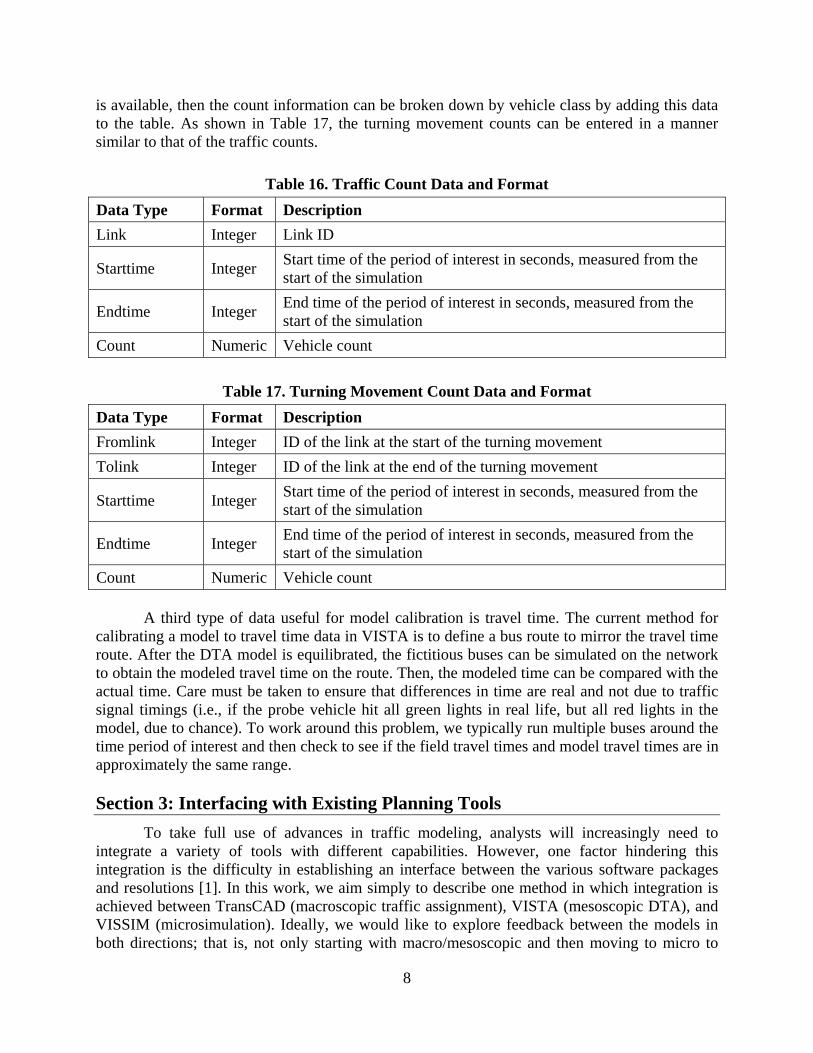
Calibration data is not needed to run DTA, but it provides a critical check on the performance of the model and can help identify errors in the network data. Typical types of calibration data are traffic counts, turning movement counts, and route travel times. Traffic counts can be uploaded to the database in the format shown in Table 16. If desired and if the data

8

is available, then the count information can be broken down by vehicle class by adding this data to the table. As shown in Table 17, the turning movement counts can be entered in a manner similar to that of the traffic counts.

Table 16. Traffic Count Data and Format


Link Integer Link ID

Starttime Integer Start time of the period of interest in seconds, measured from the start of the simulation

Endtime Integer End time of the period of interest in seconds, measured from the start of the simulation

Count Numeric Vehicle count

Table 17. Turning Movement Count Data and Format


Fromlink Integer ID of the link at the start of the turning movement

Tolink Integer ID of the link at the end of the turning movement

Starttime Integer Start time of the period of interest in seconds, measured from the start of the simulation

Endtime Integer End time of the period of interest in seconds, measured from the start of the simulation

Count Numeric Vehicle count

A third type of data useful for model calibration is travel time. The current method for calibrating a model to travel time data in VISTA is to define a bus route to mirror the travel time route. After the DTA model is equilibrated, the fictitious buses can be simulated on the network to obtain the modeled travel time on the route. Then, the modeled time can be compared with the actual time. Care must be taken to ensure that differences in time are real and not due to traffic signal timings (i.e., if the probe vehicle hit all green lights in real life, but all red lights in the model, due to chance). To work around this problem, we typically run multiple buses around the time period of interest and then check to see if the field travel times and model travel times are in approximately the same range. Section 3: Interfacing with Existing Planning Tools

To take full use of advances in traffic modeling, analysts will increasingly need to integrate a variety of tools with different capabilities. However, one factor hindering this integration is the difficulty in establishing an interface between the various software packages and resolutions [1]. In this work, we aim simply to describe one method in which integration is achieved between TransCAD (macroscopic traffic assignment), VISTA (mesoscopic DTA), and VISSIM (microsimulation). Ideally, we would like to explore feedback between the models in both directions; that is, not only starting with macro/mesoscopic and then moving to micro to

9

achieve a higher level of detail, but also using outputs from the microsimulator to further improve the meso- and macroscopic models.

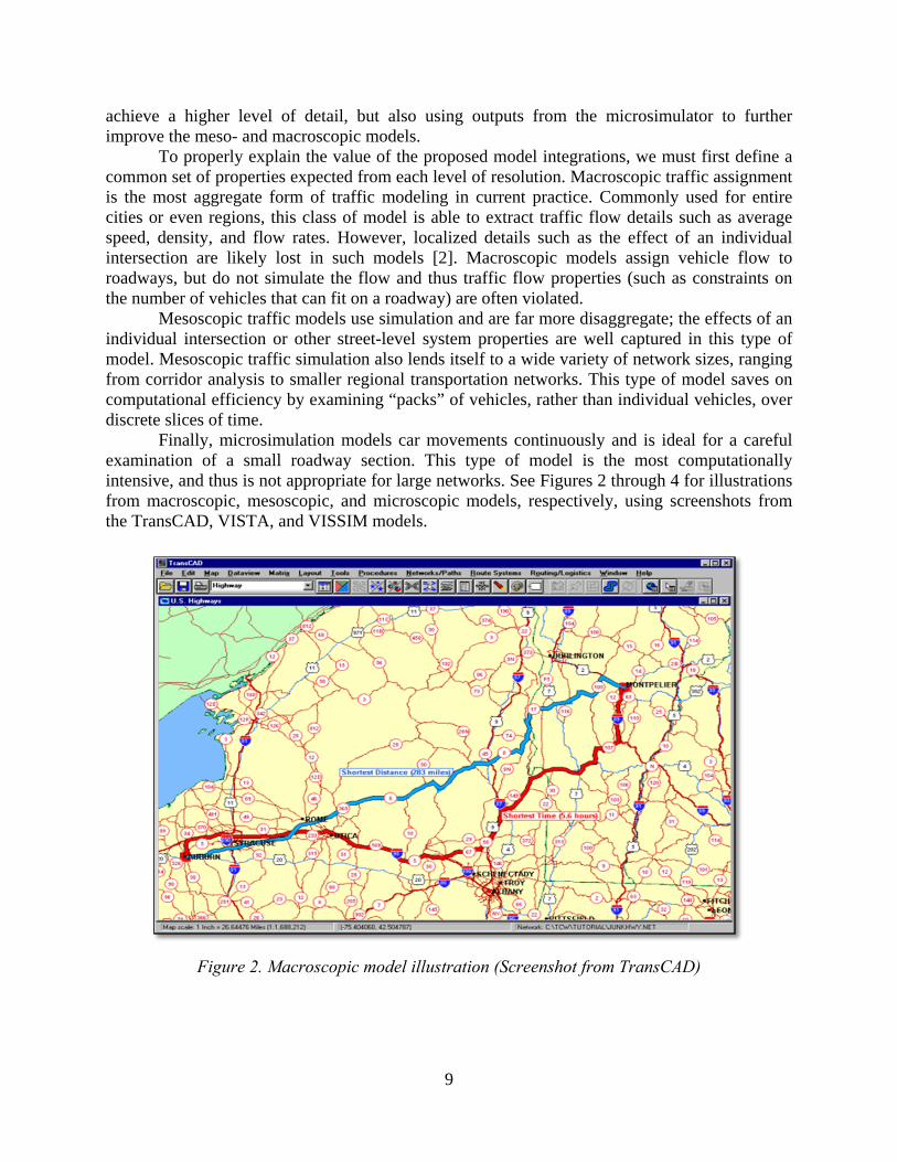
To properly explain the value of the proposed model integrations, we must first define a common set of properties expected from each level of resolution. Macroscopic traffic assignment is the most aggregate form of traffic modeling in current practice. Commonly used for entire cities or even regions, this class of model is able to extract traffic flow details such as average speed, density, and flow rates. However, localized details such as the effect of an individual intersection are likely lost in such models [2]. Macroscopic models assign vehicle flow to roadways, but do not simulate the flow and thus traffic flow properties (such as constraints on the number of vehicles that can fit on a roadway) are often violated.

Mesoscopic traffic models use simulation and are far more disaggregate; the effects of an individual intersection or other street-level system properties are well captured in this type of model. Mesoscopic traffic simulation also lends itself to a wide variety of network sizes, ranging from corridor analysis to smaller regional transportation networks. This type of model saves on computational efficiency by examining “packs” of vehicles, rather than individual vehicles, over discrete slices of time.

Finally, microsimulation models car movements continuously and is ideal for a careful examination of a small roadway section. This type of model is the most computationally intensive, and thus is not appropriate for large networks. See Figures 2 through 4 for illustrations from macroscopic, mesoscopic, and microscopic models, respectively, using screenshots from the TransCAD, VISTA, and VISSIM models.

Figure 2. Macroscopic model illustration (Screenshot from TransCAD)

10

Figure 3. Mesoscopic model illustration (screenshot from VISTA)

Figure 4. Microscopic model illustration (screenshot of VISSIM)

11

Clearly each of the described modeling resolutions has unique inputs, outputs, and network model properties. While much of this study attempts to rigorously define metrics for integrating these traffic assignment software packages, understanding the fundamental value in doing so is important. Multi-resolution traffic assignment integration will allow for each individual model to be strengthened by using beneficial output from the other models. For example, if a specific intersection’s signal timing is causing a significant bottleneck in the mesoscopic model, we can use the microscopic model to gain a more realistic understanding of the problem. Then upon analyzing the microsimulation results, we can make a more educated network update/correction within the mesoscopic model. The research team has previously conducted an application integrating a mesoscopic and microscopic model. Figures 3 and 4 demonstrate this application; the microscopic model in Figure 4 is the subset shown with the red circle of the mesoscopic model in Figure 3.

While the realm of software or model integration encompasses many needs, the most fundamental is the creation of suitable outputs from one source to be used as inputs for another. In terms of traffic assignment, this implies the necessity for consistency in the way a transportation network is defined, including schemes for naming network components such as links and nodes. Sometimes this level of consistency is not possible. For example, some microsimulation software packages use connectors to define turning movements—a concept that does not exist in meso- and macroscopic models. Such a case requires a more in-depth integration process in which we must also define a way to move from one network (or one resolution) to another. Figure 5 displays a framework for achieving integration across model platforms. The remaining portions of this section attempt to fully detail current methods we have implemented to achieve the various levels of software integration.

Figure 5. Integration framework

The remainder of this section of the guidebook will be organized as follows. Section 3.1 explores the available options compiled for achieving compatibility between TransCAD and VISTA, and Section 3.2 describes the integration between VISTA and VISSIM. In these sections

12

we will describe all of the technical and input/output data format requirements necessary to facilitate integration of the software and any problems or concerns that may be encountered during this process. 3.1 Integrating DTA and Macroscopic Models: from TransCAD to VISTA

While developing a DTA model consistent with an existing static traffic assignment model is possible, adjustments to both network representation and travel demand are typically required. This section focuses on integration of the macroscopic model TransCAD with the mesoscopic model VISTA. 3.1.1 TransCAD to VISTA: Roadway Network Representation

In TransCAD and VISTA, the naming conventions for one-way streets and for intersections can easily be made the same. The two software packages treat bidirectional links differently in two respects.

1. In TransCAD, bidirectional links are represented as one link with one ID and a column called “Dir” in the links table takes a different value depending on the direction of the link, i.e., 0 is bidirectional, 1 is one-way from the “A” node to the “B” node, and -1 is one-way from the “B” node to the “A” node. In VISTA, bidirectional links are represented as two separate links—one for each direction.

2. The other major difference in network representation is that each traffic analysis zone (TAZ) in TransCAD has one centroid that represents both the origin and destination of that TAZ. In VISTA, each TAZ has two centroids: the origin and the destination. Another consideration when transitioning a network from TransCAD to VISTA is the

values in the capacity and speed fields. In macroscopic modeling, these values are often used as calibration parameters to reflect realities such as intersection delay. In DTA modeling, these realities are modeled explicitly, so such calibration must be conducted with extreme care. For this reason, a link’s functional class is used to set its capacity and speed. The capacity is set to the appropriate saturation flow rate and the speed is set to the posted speed limit (or assumed posted speed limit for the functional class). Traffic signals are modeled explicitly, including real timing plans when available, and stop signs are accounted for through changes in the corresponding link speed limit.

Finally, network refinements may be advantageous. VISTA is a simulation-based model and it is more sensitive to the accuracy of the network representation than typical planning models. The resulting benefits include modeling of local streets in greater detail, accurately representing freeway interchanges, and detailing the lane configuration at complex intersections. While incorporating a high level of refinement throughout the network may require excessive effort, local improvements are usually implemented based on individual project needs.

The steps to prepare the link tables (“links” and “linkdetails”) for VISTA when starting from a network in TransCAD are as follows:

1. Export TransCAD links table as a text file with comma separated values.

a. Links table should have fields for the from node, to node, ID, length, direction (0, 1, or -1 as explained earlier), functional class, capacity in AB direction, capacity in BA direction, speed, and number of lanes.

14

1. Export TransCAD demand matrix to a text file for each vehicle type that will be assigned to the network.

2. Update the centroid numbers to add 100,000 to each origin centroid ID and add 200,000 to each destination centroid ID.

3. Add a column to designate the vehicle type and give a unique number to each vehicle type.

4. Concatenate the demand tables into one table containing the demand for each type.

5. Add a column, “ID,” with a unique identifier for each row. The final table should have the following columns: ID, Type, Origin, Destination, and Demand.

3.1.3 TransCAD to VISTA: Transit

In the context of VISTA, transit vehicles are represented using a specific vehicle class. These vehicles are assigned to fixed routes defined by the transit authority and are assigned stop locations and dwell times consistent with real bus stops. Five tables are needed to define transit operations in VISTA:

1. Bus_route: includes a unique ID per route and the corresponding name.

2. Bus_route_link: lists the links defining each route, and the order in which they’re traversed. Links on which bus stops are present are also identified in this table.

3. Bus_frequency: defines the frequency at which buses depart, per route. The frequency may vary throughout the assignment period.

4. Bus_period: defines periods during which the frequency of one or more routes remains constant.

5. Bus_stop: assigns a unique ID to every physical bus stop, and includes a description if desired.

Part of the information required to build the transit network may be exported from the

macroscopic model. The bus route link table may be obtained using GISDK macros, and the bus route table may be built based on the appropriate dataview in TransCAD. However, bus frequency information, and route-specific stops are typically not available in an easily transferable form from the macroscopic model. For bus stops, researchers have explored the use of Google’s GTFS (Generalized Transit Feed Spec) files. GTFS files may be processed using Excel and simple codes in C++.

3.1.4 TransCAD to VISTA: Other Needed Tables

VISTA inputs several other tables. Many of these are optional and problem-specific. The following two tables are required.

1. Vehicleclass: columns for ID for vehicle type, title of class, and description of class.

2. Demand_profile: columns for ID (consecutive number for each time slice), weight (weight assigned to each time slice), starttime (seconds), and duration (seconds).

15

a. The weights are applied to the demand in the static_od table to create the total demand in each time slice. Random number generation is then used within VISTA to assign vehicles to random times within their assigned time slice.

If diurnal factors are available from the static model, these can be used to inform the

demand profile—often a useful approach when running DTA at a regional level. When running a subnetwork, the demand profile is created when the DTA regional path flows, which are inherently dynamic and have a profile over time, are extracted to create a subnetwork demand. 3.2 Integrating DTA and Microsimulation: from VISTA to VISSIM

VISTA model outputs consist of individual vehicle trajectories. From these computing a variety of time-dependent network performance measures is possible, including intersection delay and link- or route-based travel time. However, due to the limitations of the traffic simulator implemented within the DTA framework, the resulting performance metrics do not explicitly take into account the friction introduced by weaving maneuvers or the impacts of lane widths and other intersection design characteristics. The latter may be relevant for some applications, including those concerning intersection improvements, freeway ramp design, and work-zone traffic control planning. In such cases, DTA outputs may be used to support the development of a microsimulation model, which can provide more refined performance metrics.

While microsimulation models representing present conditions may be built based on field data, the analysis of future year scenarios requires estimates of traffic volumes and turning movements, which can be obtained through DTA. Further, DTA outputs may be used to reduce the data collection needs for present year microsimulation analyses.

For this project, researchers developed a process to generate VISSIM (microsimulation) inputs from VISTA vehicle trajectory data. The following sections describe this process, as well as two alternative processes that need further research.

3.2.1 VISTA to VISSIM: Roadway Network Representation

When building a VISSIM model, the link IDs will differ from the IDs of the corresponding links in VISTA. Therefore, a lookup table relating link IDs between the two software packages is required within the conversion process. Additionally, microsimulators typically use connectors to allow vehicles to move from one link to another at intersections and at every point where road properties change. A table indicating connector ID and the corresponding IDs of the links it is connecting may be needed for the conversion process. This table can be manually retrieved from VISSIM’s .inp input file (described later in further detail) once a network has been created.

Finally, if the inputs are defined using an OD matrix (more on this later), users need to create a lookup table correlating the ID of DTA origins and destinations to that of the ODs in VISSIM.

Regarding link properties, links in VISSIM are characterized based on their number of lanes and free flow speed, which must be consistent with those used in both VISTA and TransCAD. However, turning bays and other intersection-specific characteristics, typically not modeled explicitly in the DTA approach, are included in detail in microsimulation.

16

3.2.2 VISTA to VISSIM: Vehicle Inputs

Once the VISSIM network is created, the next step necessary to integrate VISTA and VISSIM is to create an automated process of preparing output from VISTA after traffic assignment into a form that can easily be read into VISSIM. While alternative methods are available, the research team focused on a method based on vehicles and their turning movements. Alternative methodologies based on an OD matrix and based on a path set are discussed in a later section.

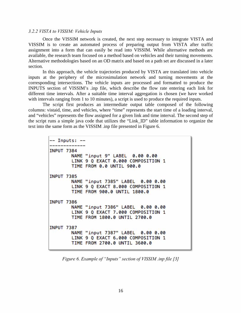
In this approach, the vehicle trajectories produced by VISTA are translated into vehicle inputs at the periphery of the microsimulation network and turning movements at the corresponding intersections. The vehicle inputs are processed and formatted to produce the INPUTS section of VISSIM’s .inp file, which describe the flow rate entering each link for different time intervals. After a suitable time interval aggregation is chosen (we have worked with intervals ranging from 1 to 10 minutes), a script is used to produce the required inputs.

The script first produces an intermediate output table composed of the following columns: vistaid, time, and vehicles, where “time” represents the start time of a loading interval, and “vehicles” represents the flow assigned for a given link and time interval. The second step of the script runs a simple java code that utilizes the “Link_ID” table information to organize the text into the same form as the VISSIM .inp file presented in Figure 6.

Figure 6. Example of “Inputs” section of VISSIM .inp file [3]

17

3.2.3 VISTA to VISSIM: Routing Decisions

The second input required for VISSIM to simulate traffic conditions is the routing decision information, which defines the percentage of turning traffic at each intersection. The routing decision data includes both route definition and the corresponding proportion of traffic. A script is used to process vista outputs and produce the turning movement data stored in an intermediate output table called “VISTA_intersection_movements.”

The “VISTA_intersection_movements” table consists of the following columns: nodeid, fromlink, tolink, and vehicles. For each turning movement in the mesoscopic simulator, the IDs for both links of a given turning movement are stored in the “fromlink” and “tolink” columns, respectively. Likewise the ID of the node connecting each link of the turning movement is stored. Finally the number of vehicles performing this movement over a given assignment period is recorded and stored in the “vehicles” column. While VISTA does not provide this table, a simple script was written to create the prescribed table by combining various pieces of standard VISTA output [4].

Based on the “routing_decisions,” “VISSIM_connectors,” and “VISTA_intersection_ movements” tables, a java code defines the routing decisions in terms of VISSIM link IDs and connectors and organizes the text into the same form as the VISSIM .inp file.

The main advantage of this technique is the relative ease of implementation, although coding the routing decisions in the microsimulator may be time-consuming if many intersections are present. Another disadvantage of our current implementation of this methodology is that the percentage of each turning movement type (e.g., 15% of drivers turn left, 75% continue straight, 10% turn right) is held constant throughout the simulation period. An interesting experiment would be to examine the possibility of making the turning percentages dynamic throughout the simulation. 3.2.4 VISTA to VISSIM: Alternative Methods for Transferring Vehicle Data

One alternative approach uses the vehicle trajectories produced by VISTA to generate an OD matrix for the network area modeled in the microsimulator. The OD ID table is then used within a script to format the VISTA OD matrix for the considered subnetwork and generate the tables required by VISSIM. Given that no path information is provided, the microsimulator has to choose the routes for all assigned vehicles. To maintain consistency with the assignment software, this approach should be applied only when a corridor-type network is modeled in the microsimulator such that only one possible path connects every specified OD pair. This methodology requires minimum data processing but can be applied only to corridor analyses.

A second alternative approach directly feeds vehicle paths from VISTA into VISSIM—the most accurate way to integrate both models. The main challenge in implementing this technique is the lack of a one-to-one correspondence between VISTA links and VISSIM links/connectors. Further research is needed to develop methods to automatically convert VISTA paths into valid VISSIM paths.

Section 4: Integrating DTA with the Four-Step Travel Model

DTA’s ability to model traffic flows at a fine time scale across a large spatial area and the availability of efficient software programs have made DTA a valuable tool to transportation planning agencies. According to a recent survey conducted by the Federal Highway

18

Administration, 42% of respondents (consisting primarily of government agencies and consulting firms) wanted to incorporate DTA into their planning analyses as soon as possible [6]. Seventy percent of respondents planned to implement DTA in the next 2 years, and 90% wanted to incorporate DTA in 3 to 4 years at the latest. Sixty-five percent of the respondents planned to eventually replace their existing static traffic assignment model with DTA [6]. Integrating DTA with an activity-based model provides an accurate, theoretically consistent (both models incorporate the temporal dimension in similar ways), state-of-the-art planning framework [7]. However, for many agencies this is too costly to implement; the traditional four-step model has been used for five decades. Therefore, combining the four-step model with DTA is a cost-effective approach (and may be the only approach) to add detailed temporal dynamics to existing planning processes. This document investigates potential ways DTA can be incorporated into the four-step model as well as the benefits and issues of such amalgamation. 4.1 Review of the Traditional Four-Step Model

The traditional four-step model, shown in Figure 7, includes four sequential processes: trip generation, trip distribution, mode choice, and traffic assignment. Trip Generation uses demographic and survey data to determine the number of trips being attracted and produced in each zone. The common practice is to divide trips into trip purpose categories. The number of trips being produced in each zone is modeled with local survey data at the household level, relating trip production with variables such as income, vehicle ownership, and household size. Linear regression is commonly used to correlate these independent variables with the number of produced trips. The linear model is used mainly for simplicity; only the average value of the independent variables for each zone is needed as input. Attracted trips can be modeled in the same fashion or can be estimated from the trip generation handbook published by the Institute of Transportation Engineers [7].

Figure 7: The traditional four-step model

Trip Distribution uses the attractions and productions from the Trip Generation step and distributes them among the traffic analysis zones in the planning area. This process results in the OD matrix, which contains the total number of trips starting in each zone and ending in every other zone. Typically, some variety of the gravity model is used. The basic gravity model is shown here:

f

19

Vij is the amount of trips originating in zone i and ending in zone j. Ai is a proportionality constant. Oi is the amount of trips originating in zone i, and Dj is the amount of trips ending in zone j. f(cij) is a function of the cost experienced by the user while traveling from zone i to zone j. The shortest path travel times from the Traffic Assignment step are typically fed back into the model to estimate f(cij).

Mode Choice converts the person trips from the Trip Distribution step into vehicle (or other mode) trips. This conversion is typically achieved through a utility function, which measures how satisfied a person is with each mode choice. Utility functions may include the comfortablity, in-vehicle and out-of-vehicle travel time, cost, and reliability of the mode. A multinomial logit (or perhaps a nested logit) is estimated from these utility functions at the household level with survey data. This result is then aggregated to the OD level to determine the mode split for each OD pair.

Traffic Assignment distributes the vehicular OD matrix from the previous step onto the transportation network using the principle of user equilibrium (PUE). PUE states that every used path between the same origin and destination must have minimal and equal travel time. In the static traffic assignment case, link performance functions are used. A link performance function relates link volumes to link travel times. Common practice is to assume the link performance function as the BPR (Bureau of Public Roads) delay function given here:

1

where t(x) is the link’s travel time with a volume of x, a free flow speed of to and a capacity of c. α and β are parameters used to fit observed data, but are usually taken as the default values of α = 0.15 and β = 4 [4].

4.2 Integration of DTA and the Four-Step Model at the Regional Level

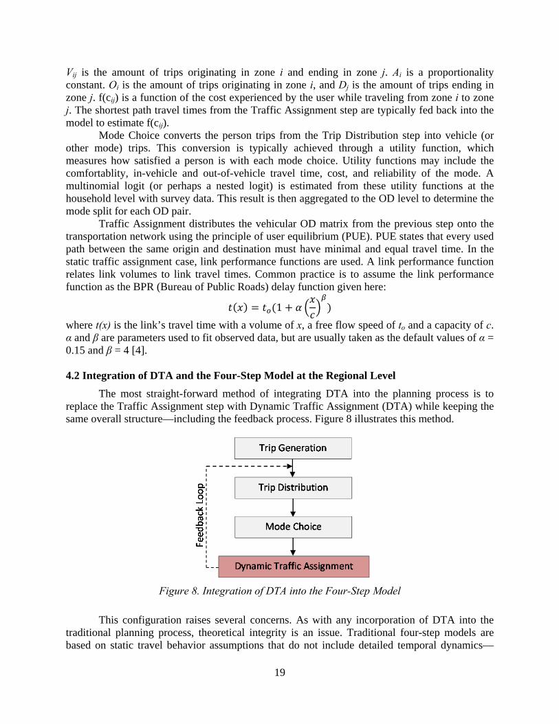
The most straight-forward method of integrating DTA into the planning process is to replace the Traffic Assignment step with Dynamic Traffic Assignment (DTA) while keeping the same overall structure—including the feedback process. Figure 8 illustrates this method.

Figure 8. Integration of DTA into the Four-Step Model

This configuration raises several concerns. As with any incorporation of DTA into the traditional planning process, theoretical integrity is an issue. Traditional four-step models are based on static travel behavior assumptions that do not include detailed temporal dynamics—

20

which is one reason why integration of DTA and activity-based models is generally preferred. The inputs necessary for the DTA process include the transportation network with known link capacities and free-flow speeds, traffic signal timings, and an OD matrix for each assignment period. Therefore, the output matrices from the Mode Choice step have to be further divided into time periods, which can be accomplished through diurnal factors and random number generation processes as discussed in Section 2.

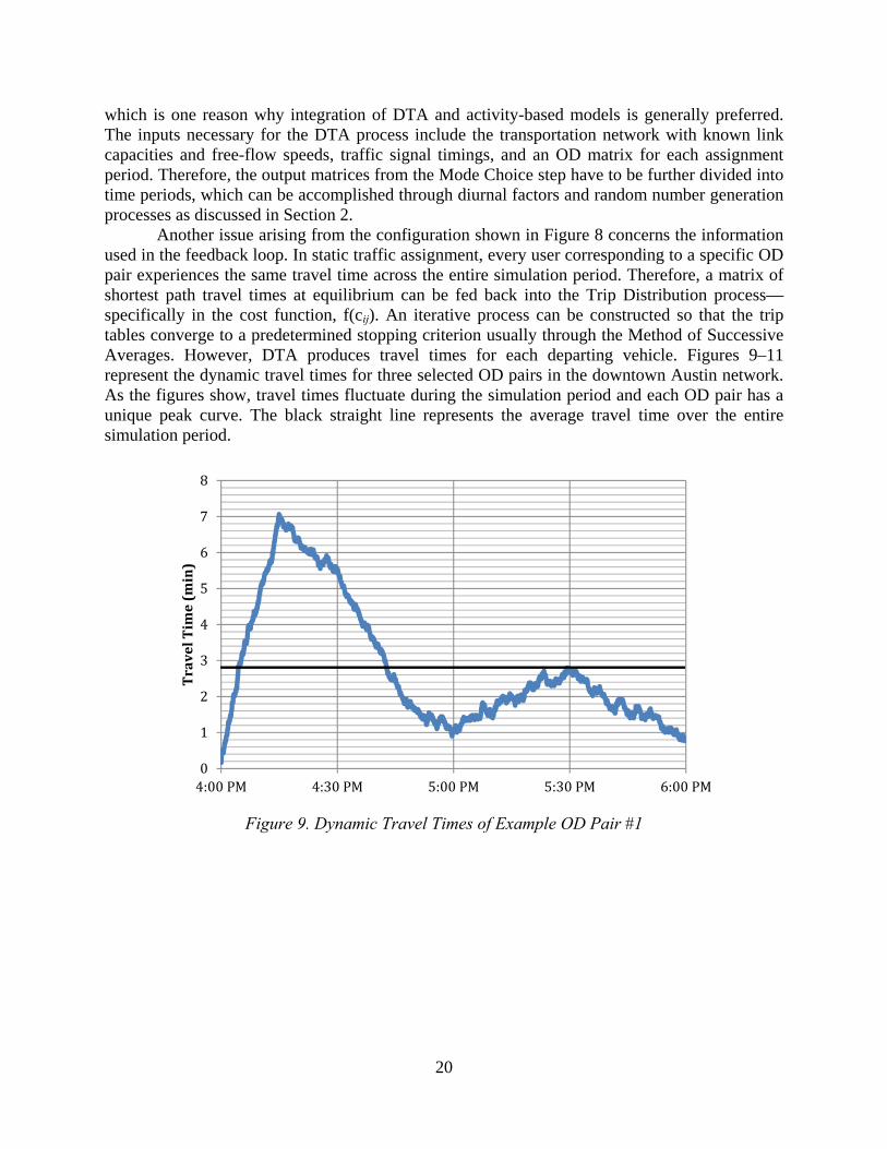
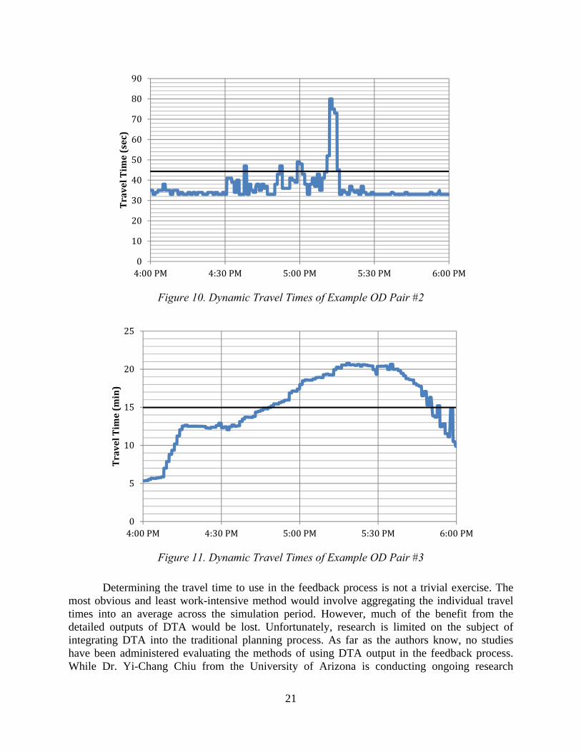
Another issue arising from the configuration shown in Figure 8 concerns the information used in the feedback loop. In static traffic assignment, every user corresponding to a specific OD pair experiences the same travel time across the entire simulation period. Therefore, a matrix of shortest path travel times at equilibrium can be fed back into the Trip Distribution process—specifically in the cost function, f(cij). An iterative process can be constructed so that the trip tables converge to a predetermined stopping criterion usually through the Method of Successive Averages. However, DTA produces travel times for each departing vehicle. Figures 9–11 represent the dynamic travel times for three selected OD pairs in the downtown Austin network. As the figures show, travel times fluctuate during the simulation period and each OD pair has a unique peak curve. The black straight line represents the average travel time over the entire simulation period.

Figure 9. Dynamic Travel Times of Example OD Pair #1

0

1

2

3

4

5

6

7

8

4:00PM 4:30PM 5:00PM 5:30PM 6:00PM

TravelTime(min)

21



Determining the travel time to use in the feedback process is not a trivial exercise. The most obvious and least work-intensive method would involve aggregating the individual travel times into an average across the simulation period. However, much of the benefit from the detailed outputs of DTA would be lost. Unfortunately, research is limited on the subject of integrating DTA into the traditional planning process. As far as the authors know, no studies have been administered evaluating the methods of using DTA output in the feedback process. While Dr. Yi-Chang Chiu from the University of Arizona is conducting ongoing research

0

10

20

30

40

50

60

70

80

90

4:00PM 4:30PM 5:00PM 5:30PM 6:00PM

TravelTime(sec)

0

5

10

15

20

25

4:00PM 4:30PM 5:00PM 5:30PM 6:00PM

TravelTime(min)

22

involving the incorporation of DTA into the Seattle planning model [5], no results have been published thus far.

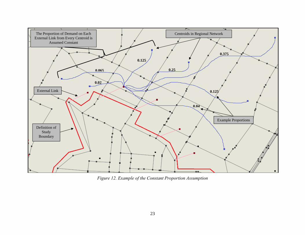
Trip Distribution typically occurs at the regional level. For example, the Capital Area Metropolitan Planning Organization (CAMPO) planning model uses the regional trip length frequency distribution in their Trip Distribution convergence process. Therefore, for a consistent, uniform feedback process, regional DTA models must be used. This may be troublesome for two reasons: (1) the long convergence time of regional DTA models (the Austin regional model takes five days to converge) and (2) agencies typically apply DTA to smaller spatial area analyses. It is possible to use sub-network outputs in the feedback process. However, certain assumptions must be made. External links of a sub-network represent all of the centroids outside of the study area. For each external link, an OD path analysis can be conducted from the regional model—meaning that every path using a particular external link can be determined. From this information, one can calculate the proportion of users from every origin/destination outside of the study area that use each external link. This proportion must be assumed constant. Essentially, we are assuming that the origins and destinations outside of the study area and the paths taken from these origins and destinations to the external links are constant. From these assumptions, one can calculate the shortest path travel time for each OD pair in the regional network while implementing DTA at the sub-network level. Figure 12 further explains the process.

23

Figure 12. Example of the Constant Proportion Assumption

External Link

Definition of Study

Boundary

Centroids in Regional Network The Proportion of Demand on Each External Link from Every Centroid is

Assumed Constant

0.25

0.125

0.125

0.375

0.04

0.02

0.065

Example Proportions

24

4.3 Integration of DTA and the Four-Step Model at the Sub-Network Level

Due to the complexity of aggregating sub-network results to the regional level, this section will focus on using DTA output in the Mode Choice step (shown in Figure 13).

Figure 13: Integration of DTA and Mode Choice

4.4 Division of the Mode Choice Model into Finer Time Intervals

As discussed in the previous section, complications arise when determining the travel time to use in the feedback process. One option of capturing travel time dynamics is to further divide the Mode Choice process into time intervals. For example, we can divide mode choice into 15-minute intervals and use the average travel time within these intervals when evaluating the utility functions. As Figure 14 shows, this approach better captures the travel time variation within the simulation period. The black solid lines represent the average travel time for each 15-minute interval. An extension of this work can be used to estimate a departure time choice model.

Figure 14: Dividing Simulation Period in 15-minute Intervals—Example OD Pair #1

0

1

2

3

4

5

6

7

8

4:00PM 4:30PM 5:00PM 5:30PM 6:00PM

TravelTime(min)

25

4.5 Introducing Travel Time Unreliability in the Mode Choice Model

The dynamic nature of each OD pair’s shortest path travel time can also be captured through a travel time unreliability measure. Travel time unreliability (i.e., the dependability of using a specific mode when traveling from a particular origin to a particular destination during a certain time period) has become an important part of the transportation planning process. Studies indicate that travel time unreliability affects mode choice [11, 12]. Using the dynamic outputs of DTA, we can measure the unreliability of the vehicular and bus mode—which can be included in the mode choice utility functions as an additional independent variable.

Several measures of travel time unreliability are used in practice, including planning time, planning time index, buffer index, coefficient of variation, congestion frequency, skew of travel-time distribution, and the unreliability indicator. Each measure can be categorized as either variance-based or skew-based. Variance-based measures are mainly used as a general system performance measure, while skew-based measures are used to evaluate alternative transportation projects. The most common skew-based measure is the skew of travel-time distribution measure (STTD) shown here:

90 50 50 10

Each OD pair varies in travel time distribution, so we can estimate the Pth percentile

using a ranking scheme. The National Institute of Standards and Technology (NIST) recommends the following equation [13]:

100

1

where N is the sample size, and P is the desired percentile. n is the rank number in the sample whose value represents the Pth percentile. Table 18 shows the STTD for each example OD pair.

Table 18: Skew of Travel-Time Distribution Measure for each Example OD Pair

Origin-Destination Pair STTD Value

Example OD Pair #1 3.667



In this example, OD pair #1 is considered the least reliable for vehicle travel and OD pair

#3 is considered the most reliable. Therefore, when conducting mode choice, the vehicle mode would be penalized for its unreliability more when considering OD pair #1 than for the other OD pairs. For completeness, incorporating an unreliability term for transit and other modes makes sense (as applicable). For example, the bus mode may experience the same degree of unreliability as the auto mode if buses do not have their own right-of-way. More research is needed to develop a cohesive method around this idea.

26

Section 5: Conclusion

Simulation-based dynamic traffic assignment software programs model route choice behavior at a fine time scale across a large spatial area. This mesoscopic level of traffic detail makes DTA a powerful and versatile tool to transportation planners. Unfortunately, there has been limited research and exploration of integrating DTA into the transportation planning process. This guidebook provides information to practitioners regarding the input data required for dynamic traffic assignment, methods and benefits of linking together macroscopic, mesoscopic, and microscopic models, and potential ways of integrating DTA into the traditional four-step planning model.

The needed inputs for dynamic traffic assignment are: the geometry and physical characteristics of the roadway system (link length, free-flow speed, capacity, etc.), signal timings and controls, transit route schedules if desired, and a dynamic origin-destination matrix. Because of the mesoscopic nature of DTA, it can be used with macroscopic regional planning and microsimulation models to create a unified system of multi-resolution traffic assignment. This integrated system can be used to identify and correct traffic problems that may have otherwise gone unnoticed. DTA can also be integrated into the traditional four-step planning process – whether it’s simply replacing static with dynamic traffic assignment or incorporating travel time unreliability in the mode choice step. The use of dynamic traffic assignment in transportation planning processes is growing and presents limitless possibilities and the potential for more efficient systems in the future. Section 6: References

1. Holyoak, Nocholas and Stazic, Branko, “Benefits of Linking Macro-Demand Forecasting Models and Microsimulations Models.” ITE Journal Volume 79, Issue 10 (2009): pp 30–39.

2. Chiu, Y.-C. et al. A Primer for Dynamic Traffic Assignment. ADB30 Transportation Network Modeling Committee, Transportation Research Board of the National Academies, Washington, D.C., 2010.

3. VISSIM 5.40-01—User Manual. PTV Karlsruhe, Germany, 2011.

4. VISTA User Guide. Vista Transport Group, Inc., 2010.

5. Chiu, Y.-C. A Primer for Dynamic Traffic Assignment Workshop. Presented at the Transportation Research Board 89th Annual Meeting, Transportation Research Board of the National Academies, Washington, D.C., 2010.

6. Lin, D.-Y., N. Eluru, S.T. Waller, and C.R. Bhat. Integration of Activity-Based Modeling and Dynamic Traffic Assignment. In Transportation Research Record: Journal of the Transportation Research Board, No. 2076, Transportation Research Board of the National Academies, Washington, D.C., 2008, pp. 52–61.

7. Institute of Transportation Engineers. Trip Generation: An ITE Information Report (8th Edition). Institute of Transportation Engineers, Washington, D.C., 2008.

8. Bureau of Public Roads. Traffic Assignment Manual. Office of Planning, Urban Planning Division, Washington, D.C., 1964.

27

9. Tung, R., Z. Wang, and Y.-C. Chiu. Integration of Dynamic Traffic Assignment in a Four-Step Model Framework—A Deployment Case Study in Seattle Model. Presented at the 3rd Conference on Innovations in Travel Modeling, 2010.

10. Sweet, M.N. and M. Chen. Does Regional Travel Time Unreliability Influence Mode Choice? Transportation, Vol. 38, 2011, pp. 625–642.

11. Bhat, C.R. and R. Sardesai. The Impact of Stop-Making and Travel Time Reliability on Commute Mode Choice. Transportation Research Part B, Vol. 40, No. 9, 2006, pp. 709–730.

12. National Institute of Standards and Technology. Engineering Statistics Handbook. National Institute of Standards and Technology, Technology Administration, U.S. Department of Commerce, Washington, D.C., 2003.

guidebook on dta data needs and interface options...

Documents