guidelines for the measurement of productivity and
TRANSCRIPT

Guidelines for the measurement of productivity and efficiency in agriculture
Guidelines for the m
easurement of productivity and efficiency in agriculture
Publication prepared in the framework of the Global Strategy to improve Agricultural and Rural Statistics
Guidelines for the measurement of productivity and efficiency in aGriculture i
Guidelines for the measurement of productivity and efficiency in agriculture
October 2018

Guidelines for the measurement of productivity and efficiency in aGricultureii
Guidelines for the measurement of productivity and efficiency in aGriculture iii
Contents
Figures and tables v
Boxes v
Acronyms vi
Acknowledgements vii
ChApter 1 IntroduCtIon 1 1.1. Importance and rationale 1
1.2. Guidelines: objectives, scope and target audience 3
1.3. Major references on productivity measurement 4
1.4. Approach and structure of the Guidelines 5
ChApter 2the ConCeptuAl FrAmework And sCope 7 2.1. General definition 7
2.2. Indicators and measurement methods 8
2.2.1. Single-factor productivity 8
2.2.2. Total Factor Productivity 9
2.3. Sources of productivity growth 13
2.3.1. Technical efficiency 13
2.3.2. Economies of scale and marginal input productivity 15
2.3.3. Technological change 16
2.4. Activities 16
2.4.1. Agricultural activities 16
2.4.2. Agricultural industry 17
2.4.3. Commodities 18
2.5. Geographical coverage 19
2.6. Household and non-household sectors 20
2.7. Agricultural output and value added 21
2.7.1. Agricultural output: three possible measures 21
2.7.2. Agricultural value added 22
2.8. Intermediate inputs and factors of production 22
2.8.1. Factors of production 23
2.8.2. Intermediate inputs 25
2.8.3. Quality and compositional changes 25
2.9. Summary of recommendations 27

Guidelines for the measurement of productivity and efficiency in aGricultureiv
Chapter 3Choosing the appropriate indiCators 29 3.1. Introduction and overview 29
3.2. Dissemination level 30
3.3. From the basic data to the indicator: the aggregation procedure 31
3.4. Levels and growth rates 33
3.4.1. Levels 34
3.4.2. Growth rates 35
3.5. Choosing from a variety of productivity indicators 35
3.5.1. Single output and single input 36
3.5.2. Multiple outputs and single input 38
3.5.3. Single output and multiple inputs 40
3.5.4. Multiple outputs and multiple inputs 41
3.6. Summary of recommendations 43
Chapter 4ColleCting data for produCtivity measurement 45 4.1. Introduction and overview 45
4.2. Agricultural output 46
4.2.1. Measurement principles 46
4.2.2. Crops 47
4.2.3. Livestock 48
4.3. Intermediate inputs 49
4.3.1. For crops 49
4.3.2. For livestock 51
4.3.3. Overhead costs 52
4.4. Factors of production 52
4.4.1. Labour 52
4.4.2. Land 56
4.4.3. Fixed assets 58
4.5. Working with aggregated time series 61
4.6. Data sources and consistency 63
4.7. Summary of recommendations 66
ConClusions 67
referenCes 68

Guidelines for the measurement of productivity and efficiency in aGriculture v
Figures and tables
Figure 1. Technical efficiency, technical change and production frontier. 14
Figure 2. Returns to scale in agriculture. 15
Figure 3. Agricultural industry and production. 17
Figure 4. Share of labour costs in total costs of production for maize in Zambia (for a 50-kg bag). 23
Figure 5. Possible data sources for the compilation of agricultural productivity. 32
Figure 6. Agriculture TFP change, by region (2001–2014). 34
Figure 7. From single-factor productivity to TFP: increasing data requirements. 35
Figure 8. Return to labour for corn production in the USA (by region, 2016). 37
Figure 9. Returns to labour in the agricultural sector in the European Union (Index, 2005=100). 39
Figure 10. Change in MFP in the agricultural sector (Italy, in percentages). 42
Figure 11. Cost structure for different agricultural commodities (Philippines, in percentages). 53
Figure 12. Imputation procedure for wages of family labour – an illustration from
a pilot study in Zambia (2018). 55
Figure 13. Extract from the section on farm assets of the Zambian Post-Harvest Questionnaire. 60
table 1. Returns to factors of production for milk in the USA. 40
Boxes
Box 1. Agricultural productivity: a general definition. 7
Box 2. Measuring TFP growth using the growth accounting method. 10
Box 3. Measuring TFP growth using the stochastic production frontier method. 11
Box 4. Accounting for changes in input quality: an illustration. 26
Box 5. Summary of recommendations. 27
Box 6. Invariance of the indicators to the aggregation procedure. 31
Box 7. Summary of recommendations. 43
Box 8. Summary of recommendations. 66

Guidelines for the measurement of productivity and efficiency in aGriculturevi
Acronyms
AeAA Agricultural and Applied Economics Association
AgrIs Agricultural Integrated Survey
Arms Agricultural Resource Management Survey
CIm Current Inventory Method
deA Data Envelopment Analysis
ers Economic Research Service
eurostAt European Statistical Office
eu European Union
FAo Food and Agriculture Organization of the United Nations
gdp Gross Domestic Product
gsArs Global Strategy to improve Agricultural and Rural Statistics
IAp International Agricultural Productivity
IsIC International Standard Industrial Classification
mFp Multifactor Productivity
ngo Non-Governmental Organization
nso National Statistical Office
oeCd Organization for Economic Co-operation and Development
pIm Perpetual Inventory Method
usd United States Dollar
usdA United States Department of Agriculture
sdg Sustainable Development Goal
snA System of National Accounts
tFp Total Factor Productivity

Guidelines for the measurement of productivity and efficiency in aGriculture vii
Acknowledgments
These Guidelines are the result of a research project undertaken within the Global Strategy to improve Agricultural and Rural Statistics (GSARS), a statistical capacity-building initiative whose Global Office is hosted by the Statistics Division of Food and Agriculture Organization of United Nations (FAO). The Guidelines build upon methodologies presented in papers, technical reports and manuals published by FAO and other organizations. They also build on the findings of technical assistance activities conducted in developing countries, especially in sub-Saharan Africa, where data collection tools have been designed and tested. These Guidelines provide recommendations on the measurement of agricultural productivity, with an emphasis on developing countries.
This document is the result of a collective endeavour of statisticians working for the GSARS and teams of the FAO Statistics Division and other organizations. Most of the research conducted within this project since 2016, as well as the drafting of the Guidelines, has been undertaken by Franck Cachia, with the support of Peter Lys and Aicha Mechri, all international consultants for FAO. Flavio Bolliger, who also participated in the technical developments, coordinated the research activity.
Special thanks are extended to the experts who peer-reviewed the Guidelines: Sun Ling Wang, Research Agricultural Economist at the Economic Research Service of the United States Department of Agriculture (USDA-ERS), and Marie Vander Donckt, international consultant for FAO’s Statistics Division. The many constructive comments and inputs received from them have greatly contributed to improve the quality of the final document. Preliminary technical documents prepared in the context of this research activity have also benefited from the review and feedback of experts from Statistics Canada, the European Union’s Joint Research Centre, the USDA and Zambia’s Central Statistical Office, through discussions held during a technical workshop on agricultural productivity measurement in Washington, D.C. in December 2016. The authors are fully responsible for any remaining errors, inconsistencies and imprecisions.
Arianna Martella coordinated the design and communication aspects.
The publication was edited by Sarah Pasetto and formatted by Laura Monopoli.
As the approaches recommended in these Guidelines are tested and implemented in an increasing number of countries, the need will arise to update, enhance or revise the methodologies and measurement frameworks. To this end, we invite the users of these Guidelines to communicate any suggestions they may have to GSARS, for incorporation in future versions of this document.

Guidelines for the measurement of productivity and efficiency in aGricultureviii

Guidelines for the measurement of productivity and efficiency in aGriculture 11
1Introduction1.1. ImportAnCe And rAtIonAle
Productivity is a measure of a performance. For any economic entity or unit, such as agricultural holdings, it can be defined as the ratio of outputs to inputs; larger values of this ratio are associated with better performance. Productivity is considered an economic concept; however, because productivity measures the amount of output produced from an existing resource base, it can also constitute a good measure of sustainability.
A reason why agricultural productivity is a subject of interest for policy-makers and analysts is that, through increased productivity, farms can better allocate scarce resources to other pursuits. At the macroeconomic level, the more efficient use of inputs and the reallocation of the surplus to other economic activities lead to higher national income. For example, an increase in labour productivity in the agricultural sector will allow part of the labour force to shift from the agricultural sector to other sectors of the economy, such as industry or services, which are generally characterized by higher productivity.
Through the measurement of agricultural productivity, farm incomes can be assessed more accurately. This link between farm productivity and incomes is explicit in the second Sustainable Development Goal (SDG) on ending hunger and malnutrition, Target 2.3 of which aims to “double, by 2030, the agricultural productivity and the incomes of small-scale food producers …”. The close relationship between agricultural productivity and farm incomes also explains why agricultural productivity and efficiency is at the centre of many of the debates, policies and measures related to food security and rural livelihoods.1 The Malabo Declaration (June 2014),2 for example, places agricultural productivity growth at the centre of Africa’s objective to achieve agriculture-led growth and fulfil targets on food and nutrition security. It states that to end hunger in Africa by 2025, at least a doubling of agricultural productivity is necessary compared to current levels.
1 While increasing productivity often leads to increasing farm income, this is not necessarily always the case: for example, a production surplus may lead to falling commodity prices and declining farm income.
2 The Malabo Declaration on Accelerated Agricultural Growth and Transformation for Shared Prosperity and Improved Livelihoods (adopt-ed during the 23rd Ordinary Session of the AU Assembly in Malabo, Equatorial Guinea, 26–27 June 2014).
Guidelines for the measurement of productivity and efficiency in aGriculture2
The importance of agricultural productivity for the performance of the farming sector and, by extension, of the entire economy justifies additional research on operational data collection and measurement frameworks for productivity and efficiency targeted to developing countries.
Despite the importance of agricultural productivity, data on this topic tends to be scarce and of poor quality, especially in developing countries. Several studies, such as Kelly et al. (1996) or Prasada Rao (1993), have noted the lack of statistics on agricultural production and productivity in developing countries. In this context, there is a need for new and improved data collection frameworks that can better measure agricultural production and the amounts of inputs used in the production processes, which are prerequisites to calculating productivity in the farming sector. These Guidelines aim to fill this data and information gap by presenting the methodological tools in a structured and logical manner, from the conceptual framework to the collection of the basic data and the construction of the indicators.
Productivity measures are typically derived from the data produced by statistical agencies and other data producers: the collection of that basic data is the starting point of a productivity measurement process that culminates with the derivation of indicators and their dissemination. A good measure of productivity therefore depends on the relevance and quality of the entire statistical process, from the design of the data collection instruments to the construction of the appropriate indicators, through to their dissemination and interpretation.

Guidelines for the measurement of productivity and efficiency in aGriculture 3
1.2. guIdelInes: oBjeCtIves, sCope And tArget AudIenCe
Objectives. These Guidelines are intended to assist countries in improving their measurement and monitoring of agricultural productivity through the provision of recommendations that are applicable to the entire data cycle, from the collection of basic data to the compilation of final indicators. These Guidelines seek to identify and present some of the best practices adopted by developed and developing countries in relation to the measurement of agricultural productivity, for the different steps of the data cycle. “Gold standard” approaches, when they exist, will be presented as examples of what countries should aim for in terms of productivity measurement and to help them benchmark their respective systems with what can be considered the “best” approach. These Guidelines also acknowledge the fact that data collection is generally costly and that a trade-off must be found between completeness, accuracy and precision, on one hand, and implementation cost, on the other hand. The approaches that are identified as providing the best cost-efficiency ratio are described and recommended as best practices for countries with limited financial and technical resources.
Scope. This document retains the traditional definition of productivity, restricted mostly to its economic dimension. The environmental and sustainability dimensions of productivity are not addressed explicitly, mainly for three reasons. The first is that another research project under the Global Strategy to improve Agricultural and Rural Statistics (hereafter, Global Strategy or GSARS) is studying the measurement of the sustainability of agricultural production in a wider sense, incorporating economic, environmental and social dimensions. To avoid overlaps and duplications, this document therefore focuses on economic productivity. The link with economic sustainability can be established directly, especially for partial productivity measures at farm level. The second reason for restricting the scope of these Guidelines to economic productivity is that the inclusion of physical and environmental resources as an input into production processes is a relatively new stream of research, particularly from the data collection and statistical perspectives. Third, most developing countries already encounter significant difficulties in measuring the economic productivity of the agricultural sector. The first and most urgent need, therefore, is to provide relevant measurement frameworks to adequately measure agricultural productivity, defined in the traditional sense, before going any further in the exploration of other dimensions.
Target audience. These Guidelines have been developed mainly for the benefit of developing countries, with an emphasis on cost-efficient approaches that can be sustainably implemented where tight technical and financial constraints apply. While the recommendations remain valid for all countries, issues such as quality adjustments or index number formulations may not have been addressed with the level of detail that countries with the most advanced statistical systems may require. These Guidelines target an audience of economists, statisticians, agro-economists and agronomists that are familiar with farm-level data collection and analysis. They are primarily intended to benefit producers of agricultural statistics at national level, such as National Statistical Offices (NSOs) or ministries of agriculture, most of which compile productivity indicators in one form or another. These Guidelines will assist them in adjusting the measurement methods to their needs, data availabilities and institutional settings.

Guidelines for the measurement of productivity and efficiency in aGriculture4
1.3. mAjor reFerenCes on produCtIvIty meAsurement
The measurement of productivity has been the subject of several academic papers, manuals and guidelines, since the foundational work of Solow (1957) and Diewert (1980). The literature review on the measurement of agricultural productivity and efficiency in agriculture, published by the Global Strategy in 2017,3 identified some of the key references in this field. These Guidelines borrow extensively from these publications. Some of the most significant references and research initiatives for the present work are listed and described below.
The manual on the measurement of productivity published by the OECD in 2001, hereinafter referred to as OECD (2001), is a guide to the various productivity measures aimed at statisticians, researchers and analysts involved in constructing industry-level productivity indicators. It presents the theoretical foundations of productivity measurement and discusses implementation and measurement issues. The objectives of the OECD manual and the present document differ in many ways: first, the former does not address the specificities of productivity measurement in the agricultural sector, which is the main purpose of these Guidelines. Second, the OECD manual mainly addresses the issue of aggregate productivity measurement (focusing, therefore, on the industry level), while the scope of the present Guidelines covers the whole data cycle, from micro-level data collection to the compilation of aggregate indicators. Third, the OECD manual is not intended to address issues that may be of specific relevance to developing countries. Nevertheless, the overall measurement approach, the conceptual and theoretical framework as well as most of the measurement principles described in the manual are relevant for the present work, and the Guidelines naturally draw heavily upon this work.
The Global Strategy’s Handbook on Agricultural Cost of Production Statistics (2016) is also of great use to these Guidelines. It provides recommendations on how agricultural outputs and inputs should be accounted for and valued, to measure the cost of production in agriculture and to compile cost and profitability indicators. As the valuation of outputs and inputs is at the centre of productivity measurement, the recommendations contained in the Handbook are used as reference for the present work.
Within the Global Strategy, a separate research line is working on sustainability indicators in agriculture, with an emphasis on land productivity, farm profitability and financial resilience. A literature review has been published on this topic (Hayati, 2017).
Finally, the prospect of adopting a broader perspective that covers the depletion of natural resources and environmental degradation in the measurement of productivity is becoming a necessity. Accounting for environmental and natural resources in the measurement of productivity may soon become required, also in developing countries. These Guidelines’ main objective is to address the large technical gap existing in developing countries regarding the measurement of traditional or economic productivity. The accounting of environmental aspects in the measurement of productivity is better addressed by organizations or groups with greater expertise in this field, such as the OECD expert group on “Measuring Environmentally Adjusted Total Factor Productivity for Agriculture”.4
3 Global Strategy to improve Agricultural and Rural Statistics (GSARS). 2017. Productivity and Efficiency Measurement in Agriculture: Literature Review and Gaps Analysis. Technical Report no. 19. Global Strategy Technical Report: Rome.
4 The report of the 2015 workshop, as well as other material produced by this expert group, may be downloaded from: http://www.oecd.org/tad/events/environmentally-adjusted-total-factor-productivity-in-agriculture.htm

Guidelines for the measurement of productivity and efficiency in aGriculture 5
1.4. ApproACh And struCture oF the guIdelInes
Approach. The objective of these Guidelines is to provide countries with recommendations on how to measure agricultural productivity, using cost-efficient approaches. This publication is designed as a “how-to” guide that aims to take statistical officers at national level through the different steps of productivity measurement, from the collection of basic data to the compilation of aggregated indicators. These Guidelines may differ from existing manuals in several ways: they extensively address data needs and data collection methods, a characteristic that is often overlooked in many publications, which tend to focus on the conceptual frameworks and mathematical formalization. It also discusses the issue of the measurement of productivity at the farm level and attempts to establish certain connections between micro- and macro-level indicators, while most publications in this field of work tend to focus on the compilation of aggregate and derived indicators, such as Total Factor Productivity (TFP). The SDGs have created a need for disaggregated productivity measurements at national level. For example, SDG Target 2.3 on productivity improvements identifies certain groups of farms for which indicators must be compiled, such as family farmers or pastoralists. This calls for bottom-up solutions to the measurement of productivity and for approaches that are capable of producing indicators with the required level of disaggregation (sectoral, geographic, etc.).
The emphasis on data requirements is justified by the fact that productivity and efficiency indicators are derived indicators, constructed from a wide variety of data sources. The relevance and quality of these indicators depend on the relevance and quality of the underlying data. These Guidelines seek to link the indicators to the data requirements as closely as possible, so that readers can quickly understand the data implications of each type of indicator. Several publications have shown that the availability of agricultural statistics in developing countries is scarce, even for basic variables such as yields, cultivated area and production. In this context, data collection approaches must be at the centre of any proposed measurement framework on agricultural productivity.
Going beyond concepts, definitions and data collection recommendations, these Guidelines also provide concrete recommendations on how to address challenges known to have a great impact on productivity measures, such as aggregating multiple inputs and outputs and accounting for quality changes. These topics have been addressed extensively in the literature from both theoretical and empirical points of view; however, applicable solutions in a context of data scarcity and limited resources are still largely missing.
Structure and outline. The Guidelines are structured in the following way: after this introduction, chapter 2 presents the conceptual framework of productivity measurement and establishes the scope in terms of the sectoral delimitations, geographical disaggregation and the coverage of outputs and inputs; chapter 3 defines different classes of productivity indicators, discusses their use, advantages and limitations and provides concrete examples; chapter 4 addresses the basic data requirements; finally, chapter 5 provides conclusions.

Guidelines for the measurement of productivity and efficiency in aGriculture6

Guidelines for the measurement of productivity and efficiency in aGriculture 77
The conceptual framework and scope2.1. generAl deFInItIon
Productivity is defined by the OECD (2001) as the relationship between the volume of output and the volume of input used to generate that output. In other words, it is a ratio of output to input. The output used for productivity measures can be in the form of goods or services and may be expressed in terms of physical quantities or volumes (values at constant prices), depending on the formulation of the indicator. Intermediate inputs and factors of production1 are the resources used to produce outputs. This definition applies to any economic sector or activity, the only difference being the nature of the outputs considered in the numerator and of the inputs in the denominator. Box 1 provides the mathematical transcription of this general definition.
1 In this document, the term “inputs” refers indifferently to intermediate inputs (seeds, agrochemicals, etc.), to factors of production (labour, etc.), or both.
Box 1. AgrICulturAl produCtIvIty: A generAl deFInItIon.
Agricultural productivity (Prod) is the ratio of outputs (O) to inputs (X), expressed either in volumes or, when possible, in physical quantities (kg, tons, etc.). For any period t:
13
2 The conceptual framework and scope
2.1. General definition
Productivity is defined by the OECD (2001) as the relationship between the volume of output and the volume of input used to generate that output. In other words, it is a ratio of output to input. The output used for productivity measures can be in the form of goods or services and may be expressed in terms of physical quantities or volumes (values at constant prices), depending on the formulation of the indicator. Intermediate inputs and factors of production5 are the resources used to produce outputs. This definition applies to any economic sector or activity, the only difference being the nature of the outputs considered in the numerator and of the inputs in the denominator. Box 1 provides the mathematical transcription of this general definition.
The interpretation of productivity as a simple ratio (productivity level) is complex when multiple outputs and inputs are considered. For this reason, productivity growth – the difference between growth in outputs and inputs – is often preferred.
Productivity is at the centre of economic growth, at the micro- (farm), meso- (sector) and macro-levels (economy-wide). Everything else equal, higher productivity results in higher production (more output is produced out of the same input base) and higher profits or income. The following section introduces the different families of productivity indicators and measurement methods.
5 In this document, the term “inputs” refers indifferently to intermediate inputs (seeds, agrochemicals, etc.), to factors of production (labour, etc.), or both.
Box 1. Agricultural productivity: a general definition.
Agricultural productivity (𝑃𝑃𝑃𝑃𝑃𝑃𝑃𝑃) is the ratio of outputs (𝑂𝑂) to inputs (𝑋𝑋), expressed either in volumes or, when possible, in physical quantities (kg, tons, etc.). For any period 𝑡𝑡:
𝑃𝑃𝑃𝑃𝑃𝑃𝑃𝑃) =𝑂𝑂)𝑋𝑋)
[1]
The growth in productivity (𝑃𝑃𝑃𝑃𝑃𝑃𝑃𝑃 ) is approximately equal to the difference between output and input growth (respectively ��𝑂 and ��𝑋):
𝑃𝑃𝑃𝑃𝑃𝑃𝑃𝑃 ) ≅ 𝑂𝑂) − 𝑋𝑋)[2]
In other words, productivity growth can be defined as the growth in output not explained by the growth in inputs, or residual growth (Solow, 1957).
The growth in productivity (Prod) is approximately equal to the difference between output and input growth respectively O and X:
13
2 The conceptual framework and scope
2.1. General definition
Productivity is defined by the OECD (2001) as the relationship between the volume of output and the volume of input used to generate that output. In other words, it is a ratio of output to input. The output used for productivity measures can be in the form of goods or services and may be expressed in terms of physical quantities or volumes (values at constant prices), depending on the formulation of the indicator. Intermediate inputs and factors of production5 are the resources used to produce outputs. This definition applies to any economic sector or activity, the only difference being the nature of the outputs considered in the numerator and of the inputs in the denominator. Box 1 provides the mathematical transcription of this general definition.
The interpretation of productivity as a simple ratio (productivity level) is complex when multiple outputs and inputs are considered. For this reason, productivity growth – the difference between growth in outputs and inputs – is often preferred.
Productivity is at the centre of economic growth, at the micro- (farm), meso- (sector) and macro-levels (economy-wide). Everything else equal, higher productivity results in higher production (more output is produced out of the same input base) and higher profits or income. The following section introduces the different families of productivity indicators and measurement methods.
5 In this document, the term “inputs” refers indifferently to intermediate inputs (seeds, agrochemicals, etc.), to factors of production (labour, etc.), or both.
Box 1. Agricultural productivity: a general definition.
Agricultural productivity (𝑃𝑃𝑃𝑃𝑃𝑃𝑃𝑃) is the ratio of outputs (𝑂𝑂) to inputs (𝑋𝑋), expressed either in volumes or, when possible, in physical quantities (kg, tons, etc.). For any period 𝑡𝑡:
𝑃𝑃𝑃𝑃𝑃𝑃𝑃𝑃) =𝑂𝑂)𝑋𝑋)
[1]
The growth in productivity (𝑃𝑃𝑃𝑃𝑃𝑃𝑃𝑃 ) is approximately equal to the difference between output and input growth (respectively ��𝑂 and ��𝑋):
𝑃𝑃𝑃𝑃𝑃𝑃𝑃𝑃 ) ≅ 𝑂𝑂) − 𝑋𝑋)[2]
In other words, productivity growth can be defined as the growth in output not explained by the growth in inputs, or residual growth (Solow, 1957).
In other words, productivity growth can be defined as the growth in output not explained by the growth in inputs, or residual growth (Solow, 1957).
2

Guidelines for the measurement of productivity and efficiency in aGriculture8
The interpretation of productivity as a simple ratio (productivity level) is complex when multiple outputs and inputs are considered. For this reason, productivity growth – the difference between growth in outputs and inputs – is often preferred.
Productivity is at the centre of economic growth, at the micro- (farm), meso- (sector) and macro-levels (economy-wide). Everything else equal, higher productivity results in higher production (more output is produced out of the same input base) and higher profits or income. The following section introduces the different families of productivity indicators and measurement methods.
2.2. IndICAtors And meAsurement methods
Productivity indicators are generally found in two forms: partial factor productivity and multifactor factor productivity. When only one input is considered, the term “single productivity indicators” is used, while “multifactor (or total factor) productivity” considers all major factors of production and intermediate inputs. These two measures are presented below.
2.2.1. single-factor productivitySingle-factor productivity measures the volume of output generated by a single input. Examples are labour productivity (such as the output per hour or day worked), land productivity (for example, output per planted area unit) or capital productivity (for example, output per machine horsepower).
Single-factor productivity indicators can be easily interpreted, understood and calculated, partly because both the numerator and denominator can be expressed in terms of physical units. They can be directly calculated from a single data source, such as a farm or household survey, and do not require auxiliary information on output or input prices, which may be more difficult to obtain than physical quantities.
However, partial productivity measures may misrepresent the performance of the farm or the farming sector in general, making it more difficult to make evidence-based analysis or policy decisions. Indeed, as the inputs are connected through the production function, the productivity of one input may be related to the use of another input. For instance, labour productivity only partially represents the intrinsic capacity of workers to produce more efficiently, because it also depends on the capital and intermediate inputs used: the use of more efficient machines requires less operator time to carry out a predetermined activity (such as harvesting 1 ha of land); the use of herbicides reduces the time spent on manual or mechanical weeding, etc. Changes in single-factor productivity reflect the combined effect of efficiency, technical change and change in the use of other inputs.
For these reasons, single-factor productivity measures cannot constitute the backbone of a statistical framework on productivity and efficiency measurement in agriculture. They must be accompanied by indicators capable of measuring the combined productivity of all the major factors of production used to produce agricultural commodities. This is the objective of Multifactor Productivity (MFP) or Total Factor Productivity (TFP).

Guidelines for the measurement of productivity and efficiency in aGriculture 9
2.2.2. total Factor productivityDefinitionTotal Factor Productivity (TFP) accounts for the contribution of all the major inputs into production and provides a measure of how efficiently they are combined in the production process. TFP provides a complete picture of productivity and, as noted by Fuglie (2015), is more closely connected to unit production costs and to market prices than partial productivity indicators. In this document, the terms TFP and MFP are used as synonyms. The difference between the two is that the latter acknowledges the fact that it is impossible to capture all inputs, and that TFP measures always capture only the main inputs. For this reason, MFP is often preferred to TFP in the technical literature.
TFP is often measured as a growth rate, as levels cannot be easily interpreted when multiple outputs and inputs are considered and aggregated. TFP growth is defined by Cornwall (1987) and many others as the change in agricultural output that is not accounted for by the change in all or several agricultural inputs, namely land, capital, labour and intermediate inputs.
Measurement methodsTFP growth can be measured using different methods, the most common being the growth accounting approach and the approaches relying on frontier analysis, grounded on econometric modelling or Data Envelopment Analysis (DEA).
The growth accounting approach. This approach is the most widely used to measure aggregate productivity growth. It consists in measuring separately the growth in total output and the growth in total inputs, the difference corresponding to TFP growth (see box 1). These Guidelines recommend using this approach for aggregate productivity measurement because it is consistent with the national accounting framework. It is also easier to understand and more easily replicable by statistical organizations than alternatives based on econometric models or linear programming.
However, the measurement of TFP using the growth accounting approach poses a certain number of challenges: first, it is demanding in terms of data, because information on quantities and prices is required for all of the outputs and the major inputs. This explains why most of the work on TFP may be found in high-income countries, where the data is available at the required level of disaggregation. Second, this method poses some conceptual challenges. As multiple outputs of heterogeneous nature are considered (cereal crops, fruits and vegetables, livestock products, etc.), changes in the composition of production (the share of the different commodities in total output) affect the growth in total output. Similarly, the growth rate in total inputs is a weighted average of the changes in individual inputs. The choice of weighting method, for example using fixed value shares over the period of analysis as in the Laspeyres or Paasche index formulation, or variable shares as in the Törnqvist-Thiel approach, has been a subject of conceptual and empirical debate. While it has been shown that the Törnqvist-Thiel approach (variable shares) is theoretically superior, it requires collecting data on prices and quantities to construct shares on a more frequent basis. The measurement of TFP growth using the growth accounting approach is explained in further detail in box 2.

Guidelines for the measurement of productivity and efficiency in aGriculture10
Box 2. meAsurIng tFp growth usIng the growth ACCountIng method.
TFP growth is the difference between total output and input growth. Fuglie (2015) derives an operational formula where TFP growth is calculated as the difference between the revenue-weighted outputs and cost-weighted inputs:
16
Econometric approaches. The most common method pertaining to this group is the so-called stochastic frontier approach. This type of approach, used for example in Rada and Valdes (2012), is briefly described in this paragraph. Box 3 provides the basics of the mathematical framework. Readers are also encouraged to consult Global Strategy (2017a) for further details and references on this and other econometric approaches. The stochastic frontier approach is a parametric method based on the estimation of production functions, that is, the parameters that connect agricultural outputs to input use (hours of labour, kg of fertilizer, etc.). A production frontier, or best-practice frontier, is determined by assuming the absence of inefficiencies in this estimated production function. The difference between the inefficient production (observed) and the frontier production (theoretical, estimated) provides a measure of technical efficiency. The change in the frontier over time can be interpreted as a measure of technological change. The rate of change in TFP between two periods can therefore be approximated as the change in the distance to the frontier (change in technical efficiency) and the movement of the frontier (technological change).
Box 2. Measuring TFP growth using the growth accounting method.
TFP growth is the difference between total output and input growth. Fuglie (2015) derives an operational formula where TFP growth is calculated as the difference between the revenue-weighted outputs and cost-weighted inputs:
𝑇𝑇𝑇𝑇𝑇𝑇 ) ≅ 5𝑅𝑅7��𝑌7,)
:
7;<
−5𝑆𝑆>��𝑋>,)
?
>;<
[3]
where 𝑅𝑅7 =𝑝𝑝7𝑦𝑦7
∑ 𝑝𝑝7𝑦𝑦77D is the share of commodity 𝑖𝑖 in total production value and 𝑆𝑆> =
𝑝𝑝>𝑥𝑥>∑ 𝑝𝑝>𝑥𝑥>>
G
is the share of input or factor of production 𝑗𝑗 in total costs of production. This decomposition is conceptually valid under the assumption that:
• The production technology is represented by a Cobb-Douglas function, which has the property of exhibiting constant returns to scale;
• Farmers adopt a profit-maximizing strategy so that the cost shares 𝑆𝑆> equal the elasticity of output to each input; and
• Markets are in long-run competitive equilibrium so that aggregate revenues ∑ 𝑝𝑝7𝑦𝑦77 are equal to aggregate costs ∑ 𝑝𝑝>𝑥𝑥>> .
This approach constitutes one of the possible ways to measure TFP using the growth accounting method. Other approaches, using different assumptions on the production technology and weights (for example, using Törnqvist indexes) may be used. The decomposition proposed by Fuglie (2015) provides countries with an operational and flexible calculation framework. Little statistical or modelling work is required (once the weighting system has been chosen), as only weights and growth rates are needed. This measurement framework also facilitates the determination of TFP growth when data is incomplete, as assumptions on weights and growth in revenues or costs can be easily incorporated into the algorithm. TFP estimates can also be easily updated as additional information is obtained on the weights, output production and input use.
where
16
Econometric approaches. The most common method pertaining to this group is the so-called stochastic frontier approach. This type of approach, used for example in Rada and Valdes (2012), is briefly described in this paragraph. Box 3 provides the basics of the mathematical framework. Readers are also encouraged to consult Global Strategy (2017a) for further details and references on this and other econometric approaches. The stochastic frontier approach is a parametric method based on the estimation of production functions, that is, the parameters that connect agricultural outputs to input use (hours of labour, kg of fertilizer, etc.). A production frontier, or best-practice frontier, is determined by assuming the absence of inefficiencies in this estimated production function. The difference between the inefficient production (observed) and the frontier production (theoretical, estimated) provides a measure of technical efficiency. The change in the frontier over time can be interpreted as a measure of technological change. The rate of change in TFP between two periods can therefore be approximated as the change in the distance to the frontier (change in technical efficiency) and the movement of the frontier (technological change).
Box 2. Measuring TFP growth using the growth accounting method.
TFP growth is the difference between total output and input growth. Fuglie (2015) derives an operational formula where TFP growth is calculated as the difference between the revenue-weighted outputs and cost-weighted inputs:
𝑇𝑇𝑇𝑇𝑇𝑇 ) ≅ 5𝑅𝑅7��𝑌7,)
:
7;<
−5𝑆𝑆>��𝑋>,)
?
>;<
[3]
where 𝑅𝑅7 =𝑝𝑝7𝑦𝑦7
∑ 𝑝𝑝7𝑦𝑦77D is the share of commodity 𝑖𝑖 in total production value and 𝑆𝑆> =
𝑝𝑝>𝑥𝑥>∑ 𝑝𝑝>𝑥𝑥>>
G
is the share of input or factor of production 𝑗𝑗 in total costs of production. This decomposition is conceptually valid under the assumption that:
• The production technology is represented by a Cobb-Douglas function, which has the property of exhibiting constant returns to scale;
• Farmers adopt a profit-maximizing strategy so that the cost shares 𝑆𝑆> equal the elasticity of output to each input; and
• Markets are in long-run competitive equilibrium so that aggregate revenues ∑ 𝑝𝑝7𝑦𝑦77 are equal to aggregate costs ∑ 𝑝𝑝>𝑥𝑥>> .
This approach constitutes one of the possible ways to measure TFP using the growth accounting method. Other approaches, using different assumptions on the production technology and weights (for example, using Törnqvist indexes) may be used. The decomposition proposed by Fuglie (2015) provides countries with an operational and flexible calculation framework. Little statistical or modelling work is required (once the weighting system has been chosen), as only weights and growth rates are needed. This measurement framework also facilitates the determination of TFP growth when data is incomplete, as assumptions on weights and growth in revenues or costs can be easily incorporated into the algorithm. TFP estimates can also be easily updated as additional information is obtained on the weights, output production and input use.
is the share of commodity i in total production value and
16
Econometric approaches. The most common method pertaining to this group is the so-called stochastic frontier approach. This type of approach, used for example in Rada and Valdes (2012), is briefly described in this paragraph. Box 3 provides the basics of the mathematical framework. Readers are also encouraged to consult Global Strategy (2017a) for further details and references on this and other econometric approaches. The stochastic frontier approach is a parametric method based on the estimation of production functions, that is, the parameters that connect agricultural outputs to input use (hours of labour, kg of fertilizer, etc.). A production frontier, or best-practice frontier, is determined by assuming the absence of inefficiencies in this estimated production function. The difference between the inefficient production (observed) and the frontier production (theoretical, estimated) provides a measure of technical efficiency. The change in the frontier over time can be interpreted as a measure of technological change. The rate of change in TFP between two periods can therefore be approximated as the change in the distance to the frontier (change in technical efficiency) and the movement of the frontier (technological change).
Box 2. Measuring TFP growth using the growth accounting method.
TFP growth is the difference between total output and input growth. Fuglie (2015) derives an operational formula where TFP growth is calculated as the difference between the revenue-weighted outputs and cost-weighted inputs:
𝑇𝑇𝑇𝑇𝑇𝑇 ) ≅ 5𝑅𝑅7��𝑌7,)
:
7;<
−5𝑆𝑆>��𝑋>,)
?
>;<
[3]
where 𝑅𝑅7 =𝑝𝑝7𝑦𝑦7
∑ 𝑝𝑝7𝑦𝑦77D is the share of commodity 𝑖𝑖 in total production value and 𝑆𝑆> =
𝑝𝑝>𝑥𝑥>∑ 𝑝𝑝>𝑥𝑥>>
G
is the share of input or factor of production 𝑗𝑗 in total costs of production. This decomposition is conceptually valid under the assumption that:
• The production technology is represented by a Cobb-Douglas function, which has the property of exhibiting constant returns to scale;
• Farmers adopt a profit-maximizing strategy so that the cost shares 𝑆𝑆> equal the elasticity of output to each input; and
• Markets are in long-run competitive equilibrium so that aggregate revenues ∑ 𝑝𝑝7𝑦𝑦77 are equal to aggregate costs ∑ 𝑝𝑝>𝑥𝑥>> .
This approach constitutes one of the possible ways to measure TFP using the growth accounting method. Other approaches, using different assumptions on the production technology and weights (for example, using Törnqvist indexes) may be used. The decomposition proposed by Fuglie (2015) provides countries with an operational and flexible calculation framework. Little statistical or modelling work is required (once the weighting system has been chosen), as only weights and growth rates are needed. This measurement framework also facilitates the determination of TFP growth when data is incomplete, as assumptions on weights and growth in revenues or costs can be easily incorporated into the algorithm. TFP estimates can also be easily updated as additional information is obtained on the weights, output production and input use.
is the share of input or factor of production j in total costs of production. This decomposition is conceptually valid under the assumption that:• The production technology is represented by a Cobb-Douglas function, which has the property of exhibiting
constant returns to scale;• Farmers adopt a profit-maximizing strategy so that the cost shares Sj equal the elasticity of output to each
input; and• Markets are in long-run competitive equilibrium so that aggregate revenues
16
Econometric approaches. The most common method pertaining to this group is the so-called stochastic frontier approach. This type of approach, used for example in Rada and Valdes (2012), is briefly described in this paragraph. Box 3 provides the basics of the mathematical framework. Readers are also encouraged to consult Global Strategy (2017a) for further details and references on this and other econometric approaches. The stochastic frontier approach is a parametric method based on the estimation of production functions, that is, the parameters that connect agricultural outputs to input use (hours of labour, kg of fertilizer, etc.). A production frontier, or best-practice frontier, is determined by assuming the absence of inefficiencies in this estimated production function. The difference between the inefficient production (observed) and the frontier production (theoretical, estimated) provides a measure of technical efficiency. The change in the frontier over time can be interpreted as a measure of technological change. The rate of change in TFP between two periods can therefore be approximated as the change in the distance to the frontier (change in technical efficiency) and the movement of the frontier (technological change).
Box 2. Measuring TFP growth using the growth accounting method.
TFP growth is the difference between total output and input growth. Fuglie (2015) derives an operational formula where TFP growth is calculated as the difference between the revenue-weighted outputs and cost-weighted inputs:
𝑇𝑇𝑇𝑇𝑇𝑇 ) ≅ 5𝑅𝑅7��𝑌7,)
:
7;<
−5𝑆𝑆>��𝑋>,)
?
>;<
[3]
where 𝑅𝑅7 =𝑝𝑝7𝑦𝑦7
∑ 𝑝𝑝7𝑦𝑦77D is the share of commodity 𝑖𝑖 in total production value and 𝑆𝑆> =
𝑝𝑝>𝑥𝑥>∑ 𝑝𝑝>𝑥𝑥>>
G
is the share of input or factor of production 𝑗𝑗 in total costs of production. This decomposition is conceptually valid under the assumption that:
• The production technology is represented by a Cobb-Douglas function, which has the property of exhibiting constant returns to scale;
• Farmers adopt a profit-maximizing strategy so that the cost shares 𝑆𝑆> equal the elasticity of output to each input; and
• Markets are in long-run competitive equilibrium so that aggregate revenues ∑ 𝑝𝑝7𝑦𝑦77 are equal to aggregate costs ∑ 𝑝𝑝>𝑥𝑥>> .
This approach constitutes one of the possible ways to measure TFP using the growth accounting method. Other approaches, using different assumptions on the production technology and weights (for example, using Törnqvist indexes) may be used. The decomposition proposed by Fuglie (2015) provides countries with an operational and flexible calculation framework. Little statistical or modelling work is required (once the weighting system has been chosen), as only weights and growth rates are needed. This measurement framework also facilitates the determination of TFP growth when data is incomplete, as assumptions on weights and growth in revenues or costs can be easily incorporated into the algorithm. TFP estimates can also be easily updated as additional information is obtained on the weights, output production and input use.
are equal to aggregate costs
16
Econometric approaches. The most common method pertaining to this group is the so-called stochastic frontier approach. This type of approach, used for example in Rada and Valdes (2012), is briefly described in this paragraph. Box 3 provides the basics of the mathematical framework. Readers are also encouraged to consult Global Strategy (2017a) for further details and references on this and other econometric approaches. The stochastic frontier approach is a parametric method based on the estimation of production functions, that is, the parameters that connect agricultural outputs to input use (hours of labour, kg of fertilizer, etc.). A production frontier, or best-practice frontier, is determined by assuming the absence of inefficiencies in this estimated production function. The difference between the inefficient production (observed) and the frontier production (theoretical, estimated) provides a measure of technical efficiency. The change in the frontier over time can be interpreted as a measure of technological change. The rate of change in TFP between two periods can therefore be approximated as the change in the distance to the frontier (change in technical efficiency) and the movement of the frontier (technological change).
Box 2. Measuring TFP growth using the growth accounting method.
TFP growth is the difference between total output and input growth. Fuglie (2015) derives an operational formula where TFP growth is calculated as the difference between the revenue-weighted outputs and cost-weighted inputs:
𝑇𝑇𝑇𝑇𝑇𝑇 ) ≅ 5𝑅𝑅7��𝑌7,)
:
7;<
−5𝑆𝑆>��𝑋>,)
?
>;<
[3]
where 𝑅𝑅7 =𝑝𝑝7𝑦𝑦7
∑ 𝑝𝑝7𝑦𝑦77D is the share of commodity 𝑖𝑖 in total production value and 𝑆𝑆> =
𝑝𝑝>𝑥𝑥>∑ 𝑝𝑝>𝑥𝑥>>
G
is the share of input or factor of production 𝑗𝑗 in total costs of production. This decomposition is conceptually valid under the assumption that:
• The production technology is represented by a Cobb-Douglas function, which has the property of exhibiting constant returns to scale;
• Farmers adopt a profit-maximizing strategy so that the cost shares 𝑆𝑆> equal the elasticity of output to each input; and
• Markets are in long-run competitive equilibrium so that aggregate revenues ∑ 𝑝𝑝7𝑦𝑦77 are equal to aggregate costs ∑ 𝑝𝑝>𝑥𝑥>> .
This approach constitutes one of the possible ways to measure TFP using the growth accounting method. Other approaches, using different assumptions on the production technology and weights (for example, using Törnqvist indexes) may be used. The decomposition proposed by Fuglie (2015) provides countries with an operational and flexible calculation framework. Little statistical or modelling work is required (once the weighting system has been chosen), as only weights and growth rates are needed. This measurement framework also facilitates the determination of TFP growth when data is incomplete, as assumptions on weights and growth in revenues or costs can be easily incorporated into the algorithm. TFP estimates can also be easily updated as additional information is obtained on the weights, output production and input use.
.
This approach constitutes one of the possible ways to measure TFP using the growth accounting method. Other approaches, using different assumptions on the production technology and weights (for example, using Törnqvist indexes) may be used. The decomposition proposed by Fuglie (2015) provides countries with an operational and flexible calculation framework. Little statistical or modelling work is required (once the weighting system has been chosen), as only weights and growth rates are needed. This measurement framework also facilitates the determination of TFP growth when data is incomplete, as assumptions on weights and growth in revenues or costs can be easily incorporated into the algorithm. TFP estimates can also be easily updated as additional information is obtained on the weights, output production and input use.
Econometric approaches. The most common method pertaining to this group is the so-called stochastic frontier approach. This type of approach, used for example in Rada and Valdes (2012), is briefly described in this paragraph. Box 3 provides the basics of the mathematical framework. Readers are also encouraged to consult Global Strategy (2017a) for further details and references on this and other econometric approaches.
The stochastic frontier approach is a parametric method based on the estimation of production functions, that is, the parameters that connect agricultural outputs to input use (hours of labour, kg of fertilizer, etc.). A production frontier, or best-practice frontier, is determined by assuming the absence of inefficiencies in this estimated production function. The difference between the inefficient production (observed) and the frontier production (theoretical, estimated) provides a measure of technical efficiency. The change in the frontier over time can be interpreted as a measure of technological change. The rate of change in TFP between two periods can therefore be approximated as the change in the distance to the frontier (change in technical efficiency) and the movement of the frontier (technological change).
The econometric approach to TFP measurement is often regarded as less data-demanding than the growth accounting approach. However, this advantage remains unclear: on one hand, this approach requires data on physical output and input quantities, while the growth accounting method requires additional information on output values and input expenses to construct the weights, which may be difficult to obtain, incomplete and of poor quality, especially in countries with limited resources for agricultural statistics. On the other hand, the estimation of TFP growth using econometric models typically requires farm-level data over several years, ideally in panel form. Auxiliary information on the explanatory factors of production inefficiencies, such as characteristics of the holder and the production environment, is also necessary.
Guidelines for the measurement of productivity and efficiency in aGriculture 11
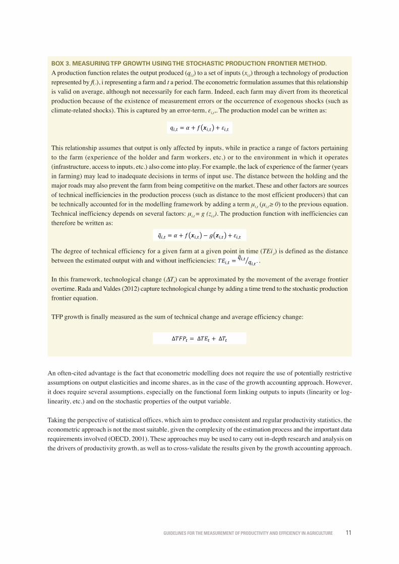
Box 3. meAsurIng tFp growth usIng the stoChAstIC produCtIon FrontIer method.
A production function relates the output produced (qi,t) to a set of inputs (xi,t) through a technology of production represented by f(.), i representing a farm and t a period. The econometric formulation assumes that this relationship is valid on average, although not necessarily for each farm. Indeed, each farm may divert from its theoretical production because of the existence of measurement errors or the occurrence of exogenous shocks (such as climate-related shocks). This is captured by an error-term, εi,t,. The production model can be written as:
17
The econometric approach to TFP measurement is often regarded as less data-demanding than the growth accounting approach. However, this advantage remains unclear: on one hand, this approach requires data on physical output and input quantities, while the growth accounting method requires additional information on output values and input expenses to construct the weights, which may be difficult to obtain, incomplete and of poor quality, especially in countries with limited resources for agricultural statistics. On the other hand, the estimation of TFP growth using econometric models typically requires farm-level data over several years, ideally in panel form. Auxiliary information on the explanatory factors of production inefficiencies, such as characteristics of the holder and the production environment, is also necessary. An often-cited advantage is the fact that econometric modelling does not require the use of potentially restrictive assumptions on output elasticities and income shares, as in the case of the
growth accounting approach. However, it does require several assumptions, especially on the functional form linking outputs to inputs (linearity or log-linearity, etc.) and on the stochastic properties of the output variable. Taking the perspective of statistical offices, which aim to produce consistent and regular productivity statistics, the econometric approach is not the most suitable, given the complexity of
Box 3. Measuring TFP growth using the stochastic production frontier method.
A production function relates the output produced (𝑞𝑞7,)) to a set of inputs (𝒙𝒙7,)) through a technology of production represented by 𝑓𝑓(. ), 𝑖𝑖 representing a farm and 𝑡𝑡 a period. The econometric formulation assumes that this relationship is valid on average, although not necessarily for each farm. Indeed, each farm may divert from its theoretical production because of the existence of measurement errors or the occurrence of exogenous shocks (such as climate-related shocks). This is captured by an error-term, 𝜀𝜀7,),. The production model can be written as:
𝑞𝑞7,) = 𝛼𝛼 + 𝑓𝑓Q𝒙𝒙7,)R + 𝜀𝜀7,)
This relationship assumes that output is only affected by inputs, while in practice a range of factors pertaining to the farm (experience of the holder and farm workers, etc.) or to the environment in which it operates (infrastructure, access to inputs, etc.) also come into play. For example, the lack of experience of the farmer (years in farming) may lead to inadequate decisions in terms of input use. The distance between the holding and the major roads may also prevent the farm from being competitive on the market. These and other factors are sources of technical inefficiencies in the production process (such as distance to the most efficient producers) that can be technically accounted for in the modelling framework by adding a term 𝜇𝜇7,) (𝜇𝜇7,) ≥ 0) to the previous equation. Technical inefficiency depends on several factors: 𝜇𝜇7,) = 𝑔𝑔Q𝒛𝒛7,)R. The production function with inefficiencies can therefore be written as:
𝑞𝑞X7,) = 𝛼𝛼 + 𝑓𝑓Q𝒙𝒙7,)R − 𝑔𝑔Q𝒛𝒛7,)R + 𝜀𝜀7,)
The degree of technical efficiency for a given farm at a given point in time (𝑇𝑇𝑇𝑇7,)) is defined as the
distance between the estimated output with and without inefficiencies: 𝑇𝑇𝑇𝑇7,) =𝑞𝑞X7,) 𝑞𝑞7,)D .
In this framework, technological change (∆𝑇𝑇)) can be approximated by the movement of the average frontier overtime. Rada and Valdes (2012) capture technological change by adding a time trend to the stochastic production frontier equation.
TFP growth is finally measured as the sum of technical change and average efficiency change:
∆𝑇𝑇𝑇𝑇𝑇𝑇) = ∆𝑇𝑇𝑇𝑇) +∆𝑇𝑇)
This relationship assumes that output is only affected by inputs, while in practice a range of factors pertaining to the farm (experience of the holder and farm workers, etc.) or to the environment in which it operates (infrastructure, access to inputs, etc.) also come into play. For example, the lack of experience of the farmer (years in farming) may lead to inadequate decisions in terms of input use. The distance between the holding and the major roads may also prevent the farm from being competitive on the market. These and other factors are sources of technical inefficiencies in the production process (such as distance to the most efficient producers) that can be technically accounted for in the modelling framework by adding a term μi,t (μi,t ≥ 0) to the previous equation. Technical inefficiency depends on several factors: μi,t = g (zi,t). The production function with inefficiencies can therefore be written as:
17
The econometric approach to TFP measurement is often regarded as less data-demanding than the growth accounting approach. However, this advantage remains unclear: on one hand, this approach requires data on physical output and input quantities, while the growth accounting method requires additional information on output values and input expenses to construct the weights, which may be difficult to obtain, incomplete and of poor quality, especially in countries with limited resources for agricultural statistics. On the other hand, the estimation of TFP growth using econometric models typically requires farm-level data over several years, ideally in panel form. Auxiliary information on the explanatory factors of production inefficiencies, such as characteristics of the holder and the production environment, is also necessary. An often-cited advantage is the fact that econometric modelling does not require the use of potentially restrictive assumptions on output elasticities and income shares, as in the case of the
growth accounting approach. However, it does require several assumptions, especially on the functional form linking outputs to inputs (linearity or log-linearity, etc.) and on the stochastic properties of the output variable. Taking the perspective of statistical offices, which aim to produce consistent and regular productivity statistics, the econometric approach is not the most suitable, given the complexity of
Box 3. Measuring TFP growth using the stochastic production frontier method.
A production function relates the output produced (𝑞𝑞7,)) to a set of inputs (𝒙𝒙7,)) through a technology of production represented by 𝑓𝑓(. ), 𝑖𝑖 representing a farm and 𝑡𝑡 a period. The econometric formulation assumes that this relationship is valid on average, although not necessarily for each farm. Indeed, each farm may divert from its theoretical production because of the existence of measurement errors or the occurrence of exogenous shocks (such as climate-related shocks). This is captured by an error-term, 𝜀𝜀7,),. The production model can be written as:
𝑞𝑞7,) = 𝛼𝛼 + 𝑓𝑓Q𝒙𝒙7,)R + 𝜀𝜀7,)
This relationship assumes that output is only affected by inputs, while in practice a range of factors pertaining to the farm (experience of the holder and farm workers, etc.) or to the environment in which it operates (infrastructure, access to inputs, etc.) also come into play. For example, the lack of experience of the farmer (years in farming) may lead to inadequate decisions in terms of input use. The distance between the holding and the major roads may also prevent the farm from being competitive on the market. These and other factors are sources of technical inefficiencies in the production process (such as distance to the most efficient producers) that can be technically accounted for in the modelling framework by adding a term 𝜇𝜇7,) (𝜇𝜇7,) ≥ 0) to the previous equation. Technical inefficiency depends on several factors: 𝜇𝜇7,) = 𝑔𝑔Q𝒛𝒛7,)R. The production function with inefficiencies can therefore be written as:
𝑞𝑞X7,) = 𝛼𝛼 + 𝑓𝑓Q𝒙𝒙7,)R − 𝑔𝑔Q𝒛𝒛7,)R + 𝜀𝜀7,)
The degree of technical efficiency for a given farm at a given point in time (𝑇𝑇𝑇𝑇7,)) is defined as the
distance between the estimated output with and without inefficiencies: 𝑇𝑇𝑇𝑇7,) =𝑞𝑞X7,) 𝑞𝑞7,)D .
In this framework, technological change (∆𝑇𝑇)) can be approximated by the movement of the average frontier overtime. Rada and Valdes (2012) capture technological change by adding a time trend to the stochastic production frontier equation.
TFP growth is finally measured as the sum of technical change and average efficiency change:
∆𝑇𝑇𝑇𝑇𝑇𝑇) = ∆𝑇𝑇𝑇𝑇) +∆𝑇𝑇)
The degree of technical efficiency for a given farm at a given point in time (TEi,t) is defined as the distance between the estimated output with and without inefficiencies:
17
The econometric approach to TFP measurement is often regarded as less data-demanding than the growth accounting approach. However, this advantage remains unclear: on one hand, this approach requires data on physical output and input quantities, while the growth accounting method requires additional information on output values and input expenses to construct the weights, which may be difficult to obtain, incomplete and of poor quality, especially in countries with limited resources for agricultural statistics. On the other hand, the estimation of TFP growth using econometric models typically requires farm-level data over several years, ideally in panel form. Auxiliary information on the explanatory factors of production inefficiencies, such as characteristics of the holder and the production environment, is also necessary. An often-cited advantage is the fact that econometric modelling does not require the use of potentially restrictive assumptions on output elasticities and income shares, as in the case of the
growth accounting approach. However, it does require several assumptions, especially on the functional form linking outputs to inputs (linearity or log-linearity, etc.) and on the stochastic properties of the output variable. Taking the perspective of statistical offices, which aim to produce consistent and regular productivity statistics, the econometric approach is not the most suitable, given the complexity of
Box 3. Measuring TFP growth using the stochastic production frontier method.
A production function relates the output produced (𝑞𝑞7,)) to a set of inputs (𝒙𝒙7,)) through a technology of production represented by 𝑓𝑓(. ), 𝑖𝑖 representing a farm and 𝑡𝑡 a period. The econometric formulation assumes that this relationship is valid on average, although not necessarily for each farm. Indeed, each farm may divert from its theoretical production because of the existence of measurement errors or the occurrence of exogenous shocks (such as climate-related shocks). This is captured by an error-term, 𝜀𝜀7,),. The production model can be written as:
𝑞𝑞7,) = 𝛼𝛼 + 𝑓𝑓Q𝒙𝒙7,)R + 𝜀𝜀7,)
This relationship assumes that output is only affected by inputs, while in practice a range of factors pertaining to the farm (experience of the holder and farm workers, etc.) or to the environment in which it operates (infrastructure, access to inputs, etc.) also come into play. For example, the lack of experience of the farmer (years in farming) may lead to inadequate decisions in terms of input use. The distance between the holding and the major roads may also prevent the farm from being competitive on the market. These and other factors are sources of technical inefficiencies in the production process (such as distance to the most efficient producers) that can be technically accounted for in the modelling framework by adding a term 𝜇𝜇7,) (𝜇𝜇7,) ≥ 0) to the previous equation. Technical inefficiency depends on several factors: 𝜇𝜇7,) = 𝑔𝑔Q𝒛𝒛7,)R. The production function with inefficiencies can therefore be written as:
𝑞𝑞X7,) = 𝛼𝛼 + 𝑓𝑓Q𝒙𝒙7,)R − 𝑔𝑔Q𝒛𝒛7,)R + 𝜀𝜀7,)
The degree of technical efficiency for a given farm at a given point in time (𝑇𝑇𝑇𝑇7,)) is defined as the
distance between the estimated output with and without inefficiencies: 𝑇𝑇𝑇𝑇7,) =𝑞𝑞X7,) 𝑞𝑞7,)D .
In this framework, technological change (∆𝑇𝑇)) can be approximated by the movement of the average frontier overtime. Rada and Valdes (2012) capture technological change by adding a time trend to the stochastic production frontier equation.
TFP growth is finally measured as the sum of technical change and average efficiency change:
∆𝑇𝑇𝑇𝑇𝑇𝑇) = ∆𝑇𝑇𝑇𝑇) +∆𝑇𝑇)
.
In this framework, technological change (∆Tt) can be approximated by the movement of the average frontier overtime. Rada and Valdes (2012) capture technological change by adding a time trend to the stochastic production frontier equation.
TFP growth is finally measured as the sum of technical change and average efficiency change:
17
The econometric approach to TFP measurement is often regarded as less data-demanding than the growth accounting approach. However, this advantage remains unclear: on one hand, this approach requires data on physical output and input quantities, while the growth accounting method requires additional information on output values and input expenses to construct the weights, which may be difficult to obtain, incomplete and of poor quality, especially in countries with limited resources for agricultural statistics. On the other hand, the estimation of TFP growth using econometric models typically requires farm-level data over several years, ideally in panel form. Auxiliary information on the explanatory factors of production inefficiencies, such as characteristics of the holder and the production environment, is also necessary. An often-cited advantage is the fact that econometric modelling does not require the use of potentially restrictive assumptions on output elasticities and income shares, as in the case of the
growth accounting approach. However, it does require several assumptions, especially on the functional form linking outputs to inputs (linearity or log-linearity, etc.) and on the stochastic properties of the output variable. Taking the perspective of statistical offices, which aim to produce consistent and regular productivity statistics, the econometric approach is not the most suitable, given the complexity of
Box 3. Measuring TFP growth using the stochastic production frontier method.
A production function relates the output produced (𝑞𝑞7,)) to a set of inputs (𝒙𝒙7,)) through a technology of production represented by 𝑓𝑓(. ), 𝑖𝑖 representing a farm and 𝑡𝑡 a period. The econometric formulation assumes that this relationship is valid on average, although not necessarily for each farm. Indeed, each farm may divert from its theoretical production because of the existence of measurement errors or the occurrence of exogenous shocks (such as climate-related shocks). This is captured by an error-term, 𝜀𝜀7,),. The production model can be written as:
𝑞𝑞7,) = 𝛼𝛼 + 𝑓𝑓Q𝒙𝒙7,)R + 𝜀𝜀7,)
This relationship assumes that output is only affected by inputs, while in practice a range of factors pertaining to the farm (experience of the holder and farm workers, etc.) or to the environment in which it operates (infrastructure, access to inputs, etc.) also come into play. For example, the lack of experience of the farmer (years in farming) may lead to inadequate decisions in terms of input use. The distance between the holding and the major roads may also prevent the farm from being competitive on the market. These and other factors are sources of technical inefficiencies in the production process (such as distance to the most efficient producers) that can be technically accounted for in the modelling framework by adding a term 𝜇𝜇7,) (𝜇𝜇7,) ≥ 0) to the previous equation. Technical inefficiency depends on several factors: 𝜇𝜇7,) = 𝑔𝑔Q𝒛𝒛7,)R. The production function with inefficiencies can therefore be written as:
𝑞𝑞X7,) = 𝛼𝛼 + 𝑓𝑓Q𝒙𝒙7,)R − 𝑔𝑔Q𝒛𝒛7,)R + 𝜀𝜀7,)
The degree of technical efficiency for a given farm at a given point in time (𝑇𝑇𝑇𝑇7,)) is defined as the
distance between the estimated output with and without inefficiencies: 𝑇𝑇𝑇𝑇7,) =𝑞𝑞X7,) 𝑞𝑞7,)D .
In this framework, technological change (∆𝑇𝑇)) can be approximated by the movement of the average frontier overtime. Rada and Valdes (2012) capture technological change by adding a time trend to the stochastic production frontier equation.
TFP growth is finally measured as the sum of technical change and average efficiency change:
∆𝑇𝑇𝑇𝑇𝑇𝑇) = ∆𝑇𝑇𝑇𝑇) +∆𝑇𝑇)
An often-cited advantage is the fact that econometric modelling does not require the use of potentially restrictive assumptions on output elasticities and income shares, as in the case of the growth accounting approach. However, it does require several assumptions, especially on the functional form linking outputs to inputs (linearity or log-linearity, etc.) and on the stochastic properties of the output variable.
Taking the perspective of statistical offices, which aim to produce consistent and regular productivity statistics, the econometric approach is not the most suitable, given the complexity of the estimation process and the important data requirements involved (OECD, 2001). These approaches may be used to carry out in-depth research and analysis on the drivers of productivity growth, as well as to cross-validate the results given by the growth accounting approach.
Guidelines for the measurement of productivity and efficiency in aGriculture12
Data Envelopment Analysis (DEA). This method also attempts to construct a production frontier to measure changes in technical efficiency and technology. However, it uses a different mathematical framework. While the stochastic production frontier is a parametric approach that requires assumptions on the functional forms f(.) and g(.)andonthedistributionoftheerrortermε,DEAconstructsthebest-practicefrontierbydetermining,througha linear optimization model, an optimal set of input-output combinations describing the production technology of a composite producer with the greatest possible efficiency. This process requires neither parametric nor stochastic assumptions. The frontier “envelops” the observed input-output combinations at farm level.2
The main advantages of using DEA to measure productivity growth are:• The absence of assumptions on the production technology of the farm or sector;• Its flexibility:
�� It can be used at any level of aggregation, from the farm to the sector, at country and international level;�� It easily accommodates multiple outputs and inputs;
• Its limited data requirements: only the quantities produced and the inputs used are necessary.
However, similarly to the econometric approach, this method is relatively complex to implement and to explain to users. Given that it is based on an optimization procedure, the results may also be unstable (small changes in the data may lead to significant changes in the results), especially in situations of data scarcity. Finally, as it is a non-parametric and non-stochastic procedure, this approach allows neither for the statistical testing of different hypotheses nor for the straightforward measurement of precision.
Taking the perspective of national data producers, DEA may be considered complementary to the growth accounting method. As for the econometric approach, it may be used to better understand and quantify the drivers of productivity growth and to cross-validate the results obtained with the growth accounting method.
Understanding the sources of productivity growth, and their interlinkages, also helps to select the most appropriate measurement methods, as well as to better interpret and make a more informed use of the results. The following section describes the different sources of productivity growth.
2 Global Strategy (2017a) provides a more detailed description of this approach as well as references to recent empirical work.
Guidelines for the measurement of productivity and efficiency in aGriculture 13
2.3. sourCes oF produCtIvIty growth
A change in farm productivity may result from one or a combination of the following effects: a change in technical efficiency, technology (including quality change), or scale economies (Fare et al., 1989). Technical efficiency is improved when existing inputs are better combined (used more efficiently). A change in production technology is characterized by the adoption of new and more efficient inputs. Scale economies are the result of decreasing marginal production costs, a situation that can be exploited by increasing output. The different explanatory factors of productivity growth and their interrelations are now described.
2.3.1. technical efficiency A farm is said to be technically inefficient if it does not produce the maximum level of output that can be expected given the resources available (Global Strategy, 2017a). An increase in technical efficiency, or a reduction in technical inefficiency, raises productivity as more output can be produced from the same set of resources.
Technical efficiency is only one of the sources of productivity growth and, therefore, should not be confused with productivity itself, as noted by Grosskopf (2002), Nishimizy and Page (1982), Fare et al. (1989) and others. Productivity measures how much output can be produced out of a given amount of resources while technical efficiency reflects “how well” a farm is able to combine the different inputs and factors of production into the production process to produce a maximum amount of output. If a farm produces the same quantity of output with fewer resources or more output with the same amount of resources, it is more productive. However, it is not necessarily more technically efficient, because this increase in productivity may be the result of the availability of better inputs (that is, technological change), for example in the form of improved seed varieties or more powerful fertilizers or pesticides, and not to a better use or combination of the existing inputs.
The definition of technical efficiency is based on the concept of production frontier, which represents the maximum output allowed by the technology. This frontier varies across countries, regions and agro-climatic zones because the technology is different, in the sense that the production conditions, such as soil types, rainfall, sunlight intensity or availability of qualified workforce, also vary. Figure 1, adapted from Rada and Valdes (2012), illustrates the conceptual difference between productivity and technical efficiency. The black and red curves represent different combinations of inputs (limited to two in this illustration) to obtain the same level of output: two different production technologies, with different productivity levels. Farms operating on the red technology require fewer inputs than those operating on the black technology to produce the same amount of output: they are more productive. Any combination of inputs on the frontiers is compatible with technical efficiency for each respective technology. Farms F2 and F1 are therefore both technically efficient if their productivity is assessed against their respective technology. Assuming that F3 has access to the same technology as F2 (for example, it is a farm of similar size located in the same locality), any move of F3 towards the black frontier represents an increase in both technical efficiency and in productivity. Assuming now that the red technology (for example, the introduction of new high-yielding or pest-resistant varieties) is accessible to F2 and F3, moving from F2 to F1 corresponds to an increase in productivity, as fewer inputs are necessary to produce a given amount of output, but not to an increase in technical efficiency: the increase in productivity is exclusively due to a technological change.

Guidelines for the measurement of productivity and efficiency in aGriculture14
FIgure 1. teChnICAl eFFICIenCy, teChnICAl ChAnge And produCtIon FrontIer.
Source: adapted from Rada and Valdes (2012).
The concepts of production frontier, technical efficiency and productivity can be illustrated by an analysis of regional differences in crop yields, a partial measure of productivity. For example, rice yields in Western Africa are estimated at 2.2 t/ha in 2014, half those of Southeast Asia (4.4 t/ha), which constitute in turn almost half the levels reached in North America (8.5 t/ha).3 This gap can be explained partly by differences in attainable yields: more conducive agro-climatic conditions in Southeast Asia, such as higher frequency, duration and intensity of rainy seasons and better soil conditions make several harvests per year in this region possible, compared to only one in most parts of sub-Saharan Africa. In addition to this technological gap, differences in the amount of inputs used and how efficiently they are combined in the production process (that is, technical efficiency) also explain why yields in regions with similar technology and production conditions (in other words, with similar attainable yields) can differ. Possible factors are higher mechanization rates, use of more productive varieties, etc.
To isolate the effect of technical efficiency from technological change and other factors, productivity growth must be decomposed into its driving factors. This decomposition is often based on the explicit construction of the production frontier, through econometric methods, data envelopment analysis or other empirical approaches. The distance of the observations (farms, enterprises) to the constructed frontier is then taken as the measure of technical efficiency, as described in section 2.4.
While the decomposition of agricultural productivity into its main driving factors is relevant from a policy point of view, it will not be addressed in detail in this publication, which focuses primarily on the measurement of agricultural productivity. The gist of the decomposition procedure, as well as references to relevant publications on this field, is given in box 3.
3 Based on data published by the Food and Agriculture Organization of the United Nations (FAO): see http://www.faostat.org
20
Source: adapted from Rada and Valdes (2012).
The concepts of production frontier, technical efficiency and productivity can be illustrated by an analysis of regional differences in crop yields, a partial measure of productivity. For example, rice yields in Western Africa are estimated at 2.2 t/ha in 2014, half those of Southeast Asia (4.4 t/ha), which constitute in turn almost half the levels reached in North America (8.5 t/ha).7 This gap can be explained partly by differences in attainable yields: more conducive agro-climatic conditions in Southeast Asia, such as higher frequency, duration and intensity of rainy seasons and better soil conditions make several harvests per year in this region possible, compared to only one in most parts of sub-Saharan Africa. In addition to this technological gap, differences in the amount of inputs used and how efficiently they are combined in the production process (that is, technical efficiency) also explain why yields in regions with similar technology and production conditions (in other words, with similar attainable yields) can differ. Possible factors are higher mechanization rates, use of more productive varieties, etc. To isolate the effect of technical efficiency from technological change and other factors, productivity growth must be decomposed into its driving factors. This decomposition is often based on the explicit construction of the production frontier, through econometric methods, data envelopment analysis or other empirical approaches. The distance of the observations (farms, enterprises) to the constructed frontier is then taken as the measure of technical efficiency, as described in section 2.4. While the decomposition of agricultural productivity into its main driving factors is relevant from a policy point of view, it will not be addressed in detail in this publication, which focuses primarily on the measurement of agricultural productivity. The gist of the decomposition procedure, as well as references to relevant publications on this field, is given in box 3.
2.5.2. Economies of scale and marginal input productivity
Economies of scale may be observed when increasing the use of all inputs leads to a proportionally higher increase in output and when unit costs decrease for each additional unit produced. Increasing (or, respectively, diminishing) marginal input productivity is when using more of a specific input leads to an increase (respectively, a decrease) in the productivity of this input (holding all the other inputs constant). For example, increasing marginal land productivity
7 Based on data published by the Food and Agriculture Organization of the United Nations (FAO): see http://www.faostat.org

Guidelines for the measurement of productivity and efficiency in aGriculture 15
2.3.2. economies of scale and marginal input productivityEconomies of scale may be observed when increasing the use of all inputs leads to a proportionally higher increase in output and when unit costs decrease for each additional unit produced. Increasing (or, respectively, diminishing) marginal input productivity is when using more of a specific input leads to an increase (respectively, a decrease) in the productivity of this input (holding all the other inputs constant). For example, increasing marginal land productivity is observed when cultivating additional land leads to an increase in average yields per hectare, which may occur for instance if the added land is of higher quality.
Increasing returns to scale, or, if only one input is considered, increasing marginal input productivity, is generally observed in situations where input use is low or inexistent. For example, using fertilizer in a field where none or little had been used in the past may, everything held equal, lead to an increase in output per unit of fertilizer used and a reduction in unit costs. However, when fertilizer is already used at levels recommended by agronomists or extension officers, adding more fertilizer to the soil will only have a marginal (or even negative) impact on yields, and lead to higher costs and lower returns per unit of land.4 Similarly, diminishing labour productivity may be observed once the hired labour increases to the point that can no longer be efficiently controlled by management. Economies of scale (that is, increasing returns to scale) may be obtained when moving from small farm sizes to larger areas, as inputs and factors of production (especially capital) can be used to the maximum of their potential. However, after a certain point, the additional area to be cultivated may require the purchase of capital (such as additional tractors or harvesters) or the use of a disproportionate amount of intermediate inputs to compensate for the lower quality of land (using large amounts of lime to reduce soil acidity, large quantities of fertilizer on low quality or degraded soil, etc.) that result in a reduction in returns, as increases in output are insufficient to cover higher costs.
Figure 2 illustrates these different phases: the returns generated by moving from A to B are higher than when moving from B to C and so forth up to E, the inflexion point after which the additional output is offset by increasing inputs costs. E can therefore be interpreted as the point at which the farm is economically efficient: before E, there is scope to increase the overall profitability by using more inputs (increasing returns to scale); after E, any additional use of input will result in lower profits (decreasing returns to scale).
FIgure 2. returns to sCAle In AgrICulture.
4 For example, higher fertilization rates contribute to increase competition from weeds, leading either to a reduction in yields of the main crop or an increase in the crop protection costs (herbicides, manual weeding) necessary to maintain yields.
22
Figure 2. Returns to scale in agriculture.
Countries with agricultural systems characterized by a low level of input use, as is typical of traditional farming, can expect economies of scale to contribute more to productivity growth. Conversely, countries with highly sophisticated and input-intensive agriculture may expect that technological change will make a greater contribution to productivity growth compared to scale and technical efficiency, as input use and combination are already close to the optimal levels.
2.5.3. Technological change
A given technology is defined by the type of inputs (intermediate inputs and factors of production in the wider sense, including agroclimatic conditions) that can be used in the production process. Different technologies are characterized by different production frontiers, or attainable production levels, as illustrated in figure 1. A change in the production technology can take the form of new and more productive inputs. The introduction of automated milking parlours in dairy production that increase the productivity of the dairy enterprise beyond previous limits is an example of technology shift in dairy production. This is an example of embodied technological change, because it is “hidden” in the capital input of the enterprise and is achieved by an investment in new equipment. For crops, the introduction of new pest-resistant varieties or varieties with shorter growth cycles are examples of technological change. The introduction of legumes and pulses in crop rotations to allow sequestration of the atmospheric nitrogen, improving soil quality and hence yields, can also be considered as a change in production technology. This last example pertains to disembodied technological change because it is created by a different way of combining inputs or using existing resources, rather than purchasing new ones.
2.6. Activities
2.6.1. Agricultural activities
As with any statistical product at national level, the scope of activities and sectors should follow international classifications and standards to ensure consistency and international comparability. The United Nations International Standard Industrial Classification of all Economic Activities (ISIC), in its latest version (revision 4), breaks down agricultural activities into:
• Crop and animal production, hunting and related service activities o Cash crops

Guidelines for the measurement of productivity and efficiency in aGriculture16
Countries with agricultural systems characterized by a low level of input use, as is typical of traditional farming, can expect economies of scale to contribute more to productivity growth. Conversely, countries with highly sophisticated and input-intensive agriculture may expect that technological change will make a greater contribution to productivity growth compared to scale and technical efficiency, as input use and combination are already close to the optimal levels.
2.3.3. technological change A given technology is defined by the type of inputs (intermediate inputs and factors of production in the wider sense, including agroclimatic conditions) that can be used in the production process. Different technologies are characterized by different production frontiers, or attainable production levels, as illustrated in figure 1.
A change in the production technology can take the form of new and more productive inputs. The introduction of automated milking parlours in dairy production that increase the productivity of the dairy enterprise beyond previous limits is an example of technology shift in dairy production. This is an example of embodied technological change, because it is “hidden” in the capital input of the enterprise and is achieved by an investment in new equipment. For crops, the introduction of new pest-resistant varieties or varieties with shorter growth cycles are examples of technological change. The introduction of legumes and pulses in crop rotations to allow sequestration of the atmospheric nitrogen, improving soil quality and hence yields, can also be considered as a change in production technology. This last example pertains to disembodied technological change because it is created by a different way of combining inputs or using existing resources, rather than purchasing new ones.
2.4. ACtIvItIes
2.4.1. Agricultural activities As with any statistical product at national level, the scope of activities and sectors should follow international classifications and standards to ensure consistency and international comparability. The United Nations International Standard Industrial Classification of all Economic Activities (ISIC), in its latest version (revision 4), breaks down agricultural activities into: • Crop and animal production, hunting and related service activities
�� Cash crops�� Food crops�� Animal production
• Forestry and logging• Fishing and aquaculture
These Guidelines focus on crops, livestock and aquaculture. Forestry, logging and fishing activities follow specific production processes that are not necessarily connected to crops and livestock. Measuring productivity for these activities requires the development of specific approaches that go beyond the scope of this publication. Hunting and gathering are not considered here due to their relatively marginal contribution to agricultural value added.

Guidelines for the measurement of productivity and efficiency in aGriculture 17
2.4.2. Agricultural industryISIC rev.4 defines the principal activity of an economic entity as the activity that contributes the most to the value added of the entity. If an entity has more than two activities, the principal activity need not represent more than 50 percent of the value added by the entity.5 The agricultural industry may be defined as the set of economic entities for which agriculture is the principal activity. Agricultural commodities can also be produced by entities that do not pertain to the agricultural industry, as a secondary or minor activity. This is the case, for example, of entities of the tourism sector that carry out horticulture or other farming activities for their own use or for recreational purposes. In national accounts, production can be viewed from the perspective of the institutional sector (household, non-household, public) of the product or of the industry. The product approach counts the entire agricultural production, independently of the industry from which it originates. The industry perspective captures the production of the units belonging to the agricultural industry, irrespective of the nature of the product (agricultural or not). Figure 3 illustrates this distinction.
Traditionally, productivity measurement and analysis focus on the agricultural industry’s production of agricultural commodities (the dark green area in figure 3). This is also the scope of these Guidelines. Secondary activities can be included only to the extent that they are inseparable from the main agricultural activity. The lending of farm machinery, farm forestry, or recreational activities related to agriculture are examples of such activities (Ball et al., 2016). Typically, the transformation of raw agricultural products (milk to butter, grain maize to maize flour, etc.) is not accounted for in the measurement of agricultural productivity because the production of the processed products can be separated from that of raw agricultural commodities, in the sense that the inputs used in their production can be differentiated.
The agricultural production of non-agricultural units (light green area in figure 3) is not taken into consideration because these activities are often minor or recreational and not representative of the aggregate agricultural production. Including it in the measurement of productivity may lead to a distortion of the estimates.
FIgure 3. AgrICulturAl Industry And AgrICulturAl produCtIon.
5 ISIC, rev.4, paragraph 57.
24
2.6.3. Commodities
The number of commodities to be included in a productivity measurement program essentially depends on the level of product disaggregation desired for the disseminated of the final indicators. The commodity coverage also affects the accuracy of the indicators.
Commodity disaggregation. Data must be collected for a given commodity if productivity indicators for such commodity are to be disseminated. However, data may not be required for every commodity if sector-wide indicators are the only outcome of the productivity measurement program. For example, if the objective is to measure TFP growth for the entire agricultural sector, the data on outputs and inputs may be restricted to the main commodities. This is a valid approach under the assumption that productivity growth for the commodities left aside is on average similar to that of the major commodities. Alternatively, data for the less important commodities can be estimated or inferred.
Productivity can be measured at different levels, from the single commodity (or farm enterprise) to the entire agricultural production. As a rule, the level of detail in the dissemination of the indicators should be dictated by user needs. If there is an interest in assessing the productivity of individual commodities (wheat, soybeans, etc.), indicators must be compiled separately for each of them. If the users are mainly interested in obtaining a global picture of farm productivity, for example to evaluate a national agricultural policy, average sector-wide productivity estimates can be constructed. The challenges associated with aggregation are addressed in detail in chapter 3.
Traditionally, productivity estimates are presented as averages for the entire agricultural industry (and, similarly, for other sectors of the economy). OECD (2001) provides guidance on the measurement of industry-level productivity growth, although not for specific commodities. Similarly, Rada and Valdes (2012) decompose aggregate agricultural productivity growth in Brazil between 1985 and 2006.
One of the reasons why aggregate or industry-wide productivity is privileged over product-specific measures is because data on input use is easier to collect for the farm than specifically for each commodity, activity or enterprise. For example, while the quantities used and expenses relating to fertilizers may be known for the holding, the application rates for each crop may be difficult to obtain from the farmer. Measuring aggregate productivity requires information on the outputs and inputs for each commodity produced by the farm: as collecting data at this level is difficult and costly, allocation procedures are often used to distribute aggregate input use to the different commodities. The academic literature on cost allocation is relatively rich and this topic

Guidelines for the measurement of productivity and efficiency in aGriculture18
2.4.3. CommoditiesThe number of commodities to be included in a productivity measurement program essentially depends on the level of product disaggregation desired for the disseminated of the final indicators. The commodity coverage also affects the accuracy of the indicators.
Commodity disaggregation. Data must be collected for a given commodity if productivity indicators for such commodity are to be disseminated. However, data may not be required for every commodity if sector-wide indicators are the only outcome of the productivity measurement program. For example, if the objective is to measure TFP growth for the entire agricultural sector, the data on outputs and inputs may be restricted to the main commodities. This is a valid approach under the assumption that productivity growth for the commodities left aside is on average similar to that of the major commodities. Alternatively, data for the less important commodities can be estimated or inferred.
Productivity can be measured at different levels, from the single commodity (or farm enterprise) to the entire agricultural production. As a rule, the level of detail in the dissemination of the indicators should be dictated by user needs. If there is an interest in assessing the productivity of individual commodities (wheat, soybeans, etc.), indicators must be compiled separately for each of them. If the users are mainly interested in obtaining a global picture of farm productivity, for example to evaluate a national agricultural policy, average sector-wide productivity estimates can be constructed. The challenges associated with aggregation are addressed in detail in chapter 3.
Traditionally, productivity estimates are presented as averages for the entire agricultural industry (and, similarly, for other sectors of the economy). OECD (2001) provides guidance on the measurement of industry-level productivity growth, although not for specific commodities. Similarly, Rada and Valdes (2012) decompose aggregate agricultural productivity growth in Brazil between 1985 and 2006.
One of the reasons why aggregate or industry-wide productivity is privileged over product-specific measures is because data on input use is easier to collect for the farm than specifically for each commodity, activity or enterprise. For example, while the quantities used and expenses relating to fertilizers may be known for the holding, the application rates for each crop may be difficult to obtain from the farmer. Measuring aggregate productivity requires information on the outputs and inputs for each commodity produced by the farm: as collecting data at this level is difficult and costly, allocation procedures are often used to distribute aggregate input use to the different commodities. The academic literature on cost allocation is relatively rich and this topic has benefited from renewed interest in recent years, with the development of Bayesian and entropy-based estimation techniques. Lips (2017), for example, uses a statistical approach based on the concept of entropy to allocate indirect input costs to the different enterprises or activities of the farm. These approaches are well adapted to academic research. However, their implementation at national scale by statistical organizations poses several technical and operational challenges.
Another reason for focusing on aggregate productivity is that the farm’s commodity mix can be considered endogenous, depending on a certain number of exogenous factors such as expected market prices or policy incentives. In this context, assessing the productivity of the entire farm (or agricultural industry) makes more economic sense. For holdings pertaining to the household sector, farm-level productivity is also more closely connected to the capacity of farmers to generate sufficient income and livelihood to sustain their household. These Guidelines recommend disseminating productivity for aggregated groups of commodities.
Accuracy. Even if the objective is to measure productivity for groups of commodities or for the agricultural sector as a whole, most of the data on output is collected for individual commodities. For crops, information on area planted, area harvested, and production are most often asked by commodity in agricultural surveys. For livestock, the number of heads and units sold is also available by animal type.

Guidelines for the measurement of productivity and efficiency in aGriculture 19
Leaving aside a share of the output may lead to an inaccurate measurement of productivity. This is clear when productivity is measured in levels, as a ratio of outputs to inputs, but also for TFP growth if differences in productivity growth can be expected between the commodities that are included and those that are left out. These Guidelines recommend ensuring a comprehensive assessment of agricultural output to minimize, distortions to productivity indicators: in addition to the main commodities, the output of the secondary or minor crops (for example those that are mixed or intercropped with a main crop, or that are cultivated in a rotation system), as well as by-products (fodder, residuals used as feed, grain set aside as seeds for the next season, etc.) should be considered. Mixed cropping is a common practice in small-scale agriculture in many developing countries. Kelly et al. (1996) indicate that the lack of proper accounting for secondary or minor crops was one of the main reasons why agricultural productivity was often underestimated in developing countries. These commodities may be key to the agricultural household’s own consumption or may represent a complementary source of cash income. For example, many farmers in southern Africa may consider maize as their main crop, yet receive complementary income from groundnuts or soybeans, for example, which are mainly cultivated for selling.
The number of commodities to cover is limited by the resources allocated to surveys and other data collection mechanisms. A trade-off must be found between completeness, targeted precision and the resources available for data collection.
2.5. geogrAphICAl CoverAge
The geographical coverage of productivity indicators depends on the targeted dissemination level and the desired level of accuracy.
Geographical disaggregation. The priority is to establish agricultural productivity indicators at national level, the geographical scale consistent with national accounts. Subnational indicators may be compiled if there is a demand by users (for example, if the country has regional economic accounts). Regionally disaggregated statistics should be envisaged only if the data is available and sufficiently reliable. Typically, when most of the data comes from an agricultural survey, the dissemination can be done at the level of statistical representativity, often the first subnational level in surveys of developing countries. Representativity at lower levels requires a significant increase in sample size and budget, which must be weighed against the benefits that this disaggregation may bring to users.
Accuracy. To obtain accurate results, the coverage of the major crops and livestock production areas should be as complete as possible. In well-designed agricultural surveys, the coverage reflects the geographical distribution of the production for the various commodities. For example, if the production of a given commodity is concentrated in a limited number of regions, data collection efforts are focused on those areas. Appropriate sampling strategies, such as multi-stage sampling with probabilities of selection proportional to size, can be used to target the areas of interest more efficiently; in other words, to better allocate the sample size to the areas of greatest importance for agricultural output. For example, if the objective is to measure the productivity of maize cultivation and if data on area planted for cereals for a large sample of farms in a given region are available from a recent survey or census, the districts with the largest maize areas can be targeted and most of the available sample allocated to them.
Guidelines for the measurement of productivity and efficiency in aGriculture20
2.6. household And non-household seCtors
In most developing countries, the agricultural sector is dominated by small and traditional farming. These farms are closely connected, and often almost confused, with the household: the holder is often the head of the household and most members of the household are involved in farming activities to some degree. Moreover, the household itself often consumes a significant share of the production, as opposed to commercial farms, which sell most of their output. Finally, most traditional farms do not have legal existence as holdings, in the sense that they are not registered as businesses. Farms with these characteristics are said to belong to the household sector. The importance of the household sector is a distinctive feature of the agricultural industry, as this characteristic is not found, or is found to a much lower extent, in other industries.
Target 2.3 of the SDG on the doubling of productivity specifically targets “small-scale food producers”. Indeed, there is a clear policy rationale for measuring productivity in the household sector separately from the non-household sector, given the close link between farm productivity and household income in family farms. The non-household sector should also be covered because it usually represents a significant share of cultivated areas, agricultural production and marketable output, even in developing countries.
The productivity measurement framework for the household sector depends on user needs, data collection tools and available sources of information. The System of National Accounts 1993 (SNA 1993) notes that “there are […] many useful ways in which the household sector may be sub-sectored and statistical agencies are advised to give due consideration to the various possibilities. More than one method may be adopted if there is a demand for different breakdowns of the household sector from different users, analysts or policy-makers.” The SNA 1993 (and subsequent releases) underlines some features of the household sector:• When the household is engaged in production for own final consumption, the value of both the output and the
consumption is imputed; the mixed income derived from the production is a form of income in kind.• The total output and value-added produced by all agricultural households may diverge significantly from the total
output and value-added of all agricultural establishments, even in developing countries. Indeed, a significant share of agricultural production may occur in established farm holdings, while, conversely, agricultural households may have significant non-agricultural output.
Considering the last point, the compilation of accounts for the agricultural household subsector is therefore no substitute for estimating total agricultural output. It must be viewed as an additional statistical product that addresses the needs of policy-makers and other users for better information on food security and income for these (often vulnerable) households.

Guidelines for the measurement of productivity and efficiency in aGriculture 21
2.7. AgrICulturAl output And vAlue Added
These Guidelines have defined agricultural productivity as the ratio of agricultural outputs to inputs. Agricultural output can be measured in several ways and the selection of the measure has implications on the calculation of productivity and its interpretation. The different measures of agricultural output and value added are presented in this section and a recommendation is made on the most appropriate measure to use in the context of productivity measurement.
2.7.1. Agricultural output: three possible measures FAO (1993) identifies three measures of output: total output, gross output and final output.
Total outputTotal agricultural output is the value of all agricultural commodities produced. This indicator is typically expressed in monetary terms, because the production of different commodities (tons of wheat, 1 000 litres of milk, etc.) must be aggregated into a single measure. In principle, other units could be chosen, such as the energetic content of each commodity (measured in kilocalories, for example). The use of the monetary unit is consistent with the valuation framework of the national accounts, reflects the economic or market value of agricultural production and is also used to measure farm income. These Guidelines, in line with the other manuals and reports on the topic, recommends measuring agricultural output in monetary (or value) terms.
Agricultural output must be valued at producer prices, that is, the prices received at the farm gate by the farmer. This price excludes transport costs and margins, even if the farmer transports the goods from the farm to the market. In practice, true producer prices are not systematically collected or estimated, and prices at the first point of sale (at the cooperative or at the wholesale market, for example) are used. A detailed discussion of the different types of prices and valuation approaches is available in FAO (1980).6
Using total output to measure agricultural productivity (that is, as the numerator of the indicator) means that the contribution of the intermediate inputs is accounted for separately in the denominator, in addition to the factors of production such as labour, land and capital. This approach may be used if there is an interest in measuring separately the contribution of intermediate inputs (such as pesticides, fertilizers, plant protection products or seeds) to productivity growth.
Gross outputFollowing FAO (1993), gross output corresponds to the total agricultural output minus the share of the output used as inputs in its own production, such as seeds for crops. This measure corresponds to the crop output available for uses other than crop production.
Final outputThe final output corresponds to the total output net of the cost of agricultural inputs, mostly seeds and animal feed. It measures the agricultural output available to other sectors of the economy and can be viewed as the produce of a “national farm”, the aggregate of the final output of all individual farms. This concept is consistent with the framework for the compilation of economic accounts for agriculture used in some countries.
6 http://www.fao.org/fileadmin/templates/ess/ess_test_folder/World_Census_Agriculture/Publications/FAO_ESDP/ESDP_16_farm_and_input_prices.pdf

Guidelines for the measurement of productivity and efficiency in aGriculture22
2.7.2. Agricultural value added The three output indicators presented above do not capture the value generated by agricultural activity because the intermediate inputs used in the production process are not deducted from the output measures (except seeds and feed, for the gross and final output). The agricultural value added corresponds to the total output minus all inputs, agricultural and non-agricultural, used in the production of agricultural commodities.
The agricultural value added measures the contribution of the agricultural sector to a country’s Gross Domestic Product (GDP) and can be used to quantify the economic returns to land, labour and capital. Agricultural value added is generally compiled on a consistent basis within a country’s system of national accounts for all industries, following the SNA, and is therefore adapted to comparisons across industries and countries.
Using the value added as the numerator of the productivity indicator enables direct measurement of the returns to factors of production such as land, labour and capital. The contribution of intermediate inputs, such as fertilizers or feed, is accounted for in the measurement of the value added.
Taking the perspective of international comparability and consistency across sectors, using the concept of value added rather than gross output to measure agricultural productivity may be more appropriate (FAO, 1993). It is also the approach recommended in these Guidelines, while acknowledging that other measures can also be used depending on the objective of the productivity measurement and the data available. OECD (2001), for instance, does not clearly recommend one measure over another but emphasizes their complementarity. Measuring the value added requires detailed and reliable information on intermediate inputs, which in many developing countries is difficult to obtain. For this reason, FAO (1993) indicates that productivity can also be measured using the concept of final output, which only requires data on outputs, seeds and feed, especially if the objective is to produce estimates that are internationally comparable. However, the advantage of the output approach over the value added in terms of data requirement does not appear to hold in practice. Indeed, if intermediate inputs are not accounted for in the numerator, they must be captured in the denominator and must be measured accordingly. Failure to account for the intermediate inputs, either in the numerator or denominator of the indicator, is likely to distort the estimation of agricultural productivity, for example by attributing productivity growth to certain factors of production, while in fact they may result from the improved efficiency of intermediate inputs.
2.8. IntermedIAte Inputs And FACtors oF produCtIon
It is important to understand that, while the choice of the output measure is important from a conceptual point of view and affects interpretation, it has no bearing on the data requirements regarding inputs. Indeed, irrespective of the approach chosen (gross output or value-added), data on quantities used and expenses on factors of production and intermediate inputs are necessary. Productivity growth being the change in output that is not accounted for by the change in inputs, the coverage of the factors of production and intermediate inputs should be as complete as possible to provide a reliable estimate of productivity.
Several publications, such as Global Strategy (2016) or AEAA (2000), have addressed the issue of input cost measurement in agriculture in greater depth than these Guidelines. The main production factors and inputs used in agriculture are introduced briefly below, while the data and information requirements for each are presented in chapter 4.
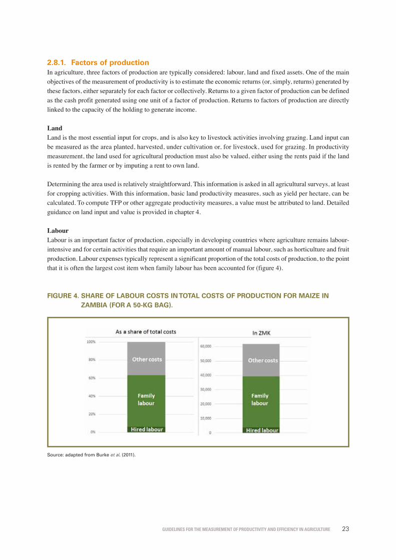
Guidelines for the measurement of productivity and efficiency in aGriculture 23
2.8.1. Factors of productionIn agriculture, three factors of production are typically considered: labour, land and fixed assets. One of the main objectives of the measurement of productivity is to estimate the economic returns (or, simply, returns) generated by these factors, either separately for each factor or collectively. Returns to a given factor of production can be defined as the cash profit generated using one unit of a factor of production. Returns to factors of production are directly linked to the capacity of the holding to generate income.
LandLand is the most essential input for crops, and is also key to livestock activities involving grazing. Land input can be measured as the area planted, harvested, under cultivation or, for livestock, used for grazing. In productivity measurement, the land used for agricultural production must also be valued, either using the rents paid if the land is rented by the farmer or by imputing a rent to own land.
Determining the area used is relatively straightforward. This information is asked in all agricultural surveys, at least for cropping activities. With this information, basic land productivity measures, such as yield per hectare, can be calculated. To compute TFP or other aggregate productivity measures, a value must be attributed to land. Detailed guidance on land input and value is provided in chapter 4.
LabourLabour is an important factor of production, especially in developing countries where agriculture remains labour-intensive and for certain activities that require an important amount of manual labour, such as horticulture and fruit production. Labour expenses typically represent a significant proportion of the total costs of production, to the point that it is often the largest cost item when family labour has been accounted for (figure 4).
FIgure 4. shAre oF lABour Costs In totAl Costs oF produCtIon For mAIze In zAmBIA (For A 50-kg BAg).
Source: adapted from Burke et al. (2011).
30
Source: adapted from Burke et al. (2011).
Labour productivity is an interesting indicator in itself and should be part of any productivity measurement program. It is relevant in many ways: labour productivity provides a sense of whether labour is being used effectively and points to potential opportunities in certain subsectors in which production could be increased with a relatively lower increase in labour input. Where there are constraints on the availability of labour, for example due to demographic shifts or loss of skills in agriculture, measures of labour productivity are likely to be important in understanding the future agricultural production possibilities.
Labour productivity measures also provide an indication of the quality of the human capital. In effect, over the longer term, labour productivity should be driven by the aim to “work smarter”, for example through exploiting improvements in the education and skills of workers, the use of improved technology and investment in assets. The retention and application of local knowledge and customs with respect to agriculture in specific locations may also be of particular significance.
Fixed assets
Agricultural assets (or fixed assets or capital) can be defined as inputs that provide services over multiple agricultural seasons, as opposed to intermediate inputs such as seeds or feed that have a one-time effect. Farm machinery and equipment, such as planters, harvesters, threshers or equipment used to apply fertilizers and phytosanitary products, are used for a wide array of cropping activities. Feed mixers, milking machines or insemination equipment are examples of assets used in livestock production. Assets also include buildings and infrastructure used for agricultural purposes, such as storage facilities, animal shelters and irrigation systems. Following the definition provided by the SNA 2008, cultivated biological resources, such as animals used as draught power or used for production (milking cows, sheep for wool, etc.) as well as tree plantations (fruit trees, managed forest plantations, etc.) can also be considered as assets. The biological asset base may, however, be more unstable than for other fixed assets, thus generating complexity in the measurement of the capital stock. For example, an animal may be used as a fixed asset one day and sold to a slaughterhouse the other day, depending on the needs of the farmer. This also creates complexities in the depreciation process (highly variable asset life and service schedules), especially in developing countries where the distinction between biological assets and final products may be less clear-cut. For these reasons, this document will focus on non-biological assets (machinery, equipment, infrastructure, etc.), without a major loss of generality, as the overall measurement process may be also applied to cultivated biological assets.
Accounting for asset ownership in productivity measurement may not be the priority in countries where agriculture is largely traditional, small-scale and characterized by a low mechanization rate. The amount of data to be gathered (type of assets, characteristics, etc.) and the difficulties encountered in estimating a service flow of the corresponding assets may not be justified.

Guidelines for the measurement of productivity and efficiency in aGriculture24
Labour productivity is an interesting indicator in itself and should be part of any productivity measurement program. It is relevant in many ways: labour productivity provides a sense of whether labour is being used effectively and points to potential opportunities in certain subsectors in which production could be increased with a relatively lower increase in labour input. Where there are constraints on the availability of labour, for example due to demographic shifts or loss of skills in agriculture, measures of labour productivity are likely to be important in understanding the future agricultural production possibilities.
Labour productivity measures also provide an indication of the quality of the human capital. In effect, over the longer term, labour productivity should be driven by the aim to “work smarter”, for example through exploiting improvements in the education and skills of workers, the use of improved technology and investment in assets. The retention and application of local knowledge and customs with respect to agriculture in specific locations may also be of particular significance.
Fixed assetsAgricultural assets (or fixed assets or capital) can be defined as inputs that provide services over multiple agricultural seasons, as opposed to intermediate inputs such as seeds or feed that have a one-time effect. Farm machinery and equipment, such as planters, harvesters, threshers or equipment used to apply fertilizers and phytosanitary products, are used for a wide array of cropping activities. Feed mixers, milking machines or insemination equipment are examples of assets used in livestock production. Assets also include buildings and infrastructure used for agricultural purposes, such as storage facilities, animal shelters and irrigation systems. Following the definition provided by the SNA 2008, cultivated biological resources, such as animals used as draught power or used for production (milking cows, sheep for wool, etc.) as well as tree plantations (fruit trees, managed forest plantations, etc.) can also be considered as assets. The biological asset base may, however, be more unstable than for other fixed assets, thus generating complexity in the measurement of the capital stock. For example, an animal may be used as a fixed asset one day and sold to a slaughterhouse the other day, depending on the needs of the farmer. This also creates complexities in the depreciation process (highly variable asset life and service schedules), especially in developing countries where the distinction between biological assets and final products may be less clear-cut. For these reasons, this document will focus on non-biological assets (machinery, equipment, infrastructure, etc.), without a major loss of generality, as the overall measurement process may be also applied to cultivated biological assets.
Accounting for asset ownership in productivity measurement may not be the priority in countries where agriculture is largely traditional, small-scale and characterized by a low mechanization rate. The amount of data to be gathered (type of assets, characteristics, etc.) and the difficulties encountered in estimating a service flow of the corresponding assets may not be justified. Nevertheless, given the move towards the increased mechanization of agriculture in developing countries and the importance of embodied technical change (technical change embedded in the purchase of new assets) for productivity growth, proper accounting for assets is likely to contribute to a better appraisal of productivity growth and better understanding of its driving factors.
The role of capital assets in agricultural production and productivity is also fundamental, given the possibilities of substitution between capital and labour, a well-known phenomenon that shaped agriculture in the developed world in the nineteenth and twentieth centuries: investments in more efficient farm assets contribute to freeing part of the labour force for other sectors of the economy, which may be potentially more productive and profitable, such as the industry or services, with a positive impact on the aggregate creation of wealth.

Guidelines for the measurement of productivity and efficiency in aGriculture 25
2.8.2. Intermediate inputsIntermediate inputs in agriculture are those inputs that are entirely or almost entirely used up during one agricultural season. For crops, the major intermediate inputs include seeds, fertilizers, phytosanitary products, irrigation water, fuel (for machinery and vehicles) and electricity. For livestock, typical intermediate inputs are feed, water used for animals, drugs, vaccines and other veterinary products, as well as electricity and fuel for buildings and machinery.
The data may be collected from a variety of sources: agricultural surveys, input supplier surveys and private or administrative sources.
2.8.3. Quality and compositional changes
Changes in input qualityChanges in the quality of inputs affect productivity growth. The examples are numerous: substituting a hectare of irrigated land for a hectare of non-irrigated land increases crop yields; using more qualified and experienced agricultural workers generally results in a greater output per unit of labour; using more fuel-efficient machines increases capital productivity. Changes in the quality of intermediate inputs, such as fertilizers or pesticides, may also be significant and contribute to raising productivity. For example, Nehring (2013) show how the potency of the herbicides commonly used for soybean in the United States rose from 1996 to 2006: 1 litre of herbicides used in 2006 had a greater impact on yields than 1 litre used in 1996.
Quality changes in inputs may result from two factors: modifications in the quality of individual inputs (individual effect) and shifts of the input mix towards more efficient inputs (structural effect or compositional change). For example, agricultural productivity may benefit from an overall increase in the level of education of the workforce employed in agriculture (individual effect), as well as from a higher share of educated workforce in total farm labour (structural effect). Similarly, increases in the overall potency and selectivity of individual pesticides or shifts of expense patterns towards pesticides with higher potency and selectivity can both be regarded as quality changes leading to higher productivity.
Changes in the quality of factors of production and intermediate inputs must be accounted for when measuring MFP, because inputs of different quality levels have different marginal productivities, and therefore different prices, which must be accounted for in the aggregation process. For example, when compiling a measure of land input, planted area cannot be aggregated without considering the fact that part of the land is irrigated and part is not. Consider an example where planted area remains stable at 100 ha; however, the share of irrigated land increases from 25 percent to 50 percent. If it is assumed that rents or imputed rents are also stable between the two periods, when in fact they should be higher because irrigated land is more expensive than non-irrigated land, the value of land input is being underestimated and, therefore, MFP is overestimated. Similarly, adding kilograms or litres of fertilizers with different potency levels (or, similarly, using one price to value different fertilizers) leads to a distortion in the measurement of volumes of inputs and, therefore, to biased productivity estimates.
Typically, quality adjustments are made through prices, as these normally reflect differences in marginal productivity and efficiency of inputs. Quality differences may be taken into account in two ways: the first, which may be referred to as ex-ante adjustment, consists in treating inputs with different quality attributes as separate goods or services, and collecting data on quantities and prices for each item. This allows for the tracking of quality changes, compositional changes and the appearance of new products from the data collection phase. Taking the example of labour input, this requires collecting data on the days or hours worked by each category of worker, as well as the corresponding wages. However, in practice, data compilers are faced with more or less aggregated data on values or quantities, and detailed price information may be difficult to obtain. This is why ex-post adjustments are often required to construct quality adjusted series for the inputs and factors of production. Typically, these adjustments are

Guidelines for the measurement of productivity and efficiency in aGriculture26
made by estimating price as a function of a set of quality attributes (a method known as hedonic regression). These estimated (or quality-adjusted) prices are then used to determine the adjusted quantity series. This is the approach used for example by Nehring (2013) to construct a quality-adjusted time series of pesticide use from 1948 to 2011 for the United States of America. A different method is used by Rada and Valdes (2012), based on the approach described in Fuglie (2015), because of the absence of rental rates for the different land groups (temporary cropland, permanent crop, pasture, etc.): the authors formed a temporary cropland-equivalent series using weights representing the productivity of each land class relative to temporary cropland.
Differentiating inputs and factors of production by quality level from the data collection phase is the approach recommended in these Guidelines. Although it may result in higher data collection requirements, as information on quantities and prices must be collected for each class of inputs, it is easier to implement that the alternative ex-post adjustments based on econometric modelling.
Changes in output qualityOutputs are also affected by quality and compositional changes. Adjusting output volumes for quality changes is a subject that has not been studied as often by the literature; still, it is a topic of equivalent importance in the context of productivity measurement. Data on output quantities and prices is usually available with a greater level of detail than for inputs, thus allowing for distinguishing and measuring outputs by grade and quality levels. Therefore, there is less need to make ex-post adjustments for quality changes.
Box 4. ACCountIng For ChAnges In Input QuAlIty: An IllustrAtIon.
The impact of input quality changes on productivity measurement can be illustrated by the following fictive example. Let us assume that labour input for a farm is estimated at 100 person-days in two periods (1 and 2) and that output is estimated at 200 for both periods.
Without additional information on the type of labour used, we can conclude that labour productivity has been stable from period 1 to 2. However, if we consider that in period 2, a higher proportion of specialized workers was employed, labour productivity has in fact fallen.
These quality or compositional changes can be accounted for in two ways: the first is to use the corresponding wages of the different types of workers. The average daily wages in period 2 should be higher given the higher proportion of skilled workers: assuming an average daily wage of 1 USD in period 1, the average for period 2 may be, for example, 1.2 (expressed in terms of period 1 prices). Labour input is therefore valued at 100 in period 1 and 120 in period 2, corresponding to a reduction in labour productivity (200/100 > 200/120).
The second approach is to construct a unique labour-input series, using one category of worker as reference. For example, assuming that a skilled worker yields 25 percent more than an unskilled worker, each unit of time worked by each category of worker is converted into unskilled worker equivalents. In our example, if a higher proportion of skilled workers is used in period 2, the adjusted labour-input series will be higher than 100, reflecting a declining labour productivity.
This example is given only to illustrate the quality adjustment process and does not seek to reflect reality. Indeed, employing a higher proportion of skilled workers should increase output (above 100), as a reflection of the higher marginal productivity of these workers, and therefore compensate for their higher cost at least in part. While this may be observed in the long run or can be assumed in theory, in practice, over the short- to medium-term this equivalence (between the increased cost and increased marginal productivity) may not hold.

Guidelines for the measurement of productivity and efficiency in aGriculture 27
2.9. summAry oF reCommendAtIons
Box 5. summAry oF reCommendAtIons.
Productivity indicators• Using TFP is recommended to measure aggregate productivity in agriculture.• TFP may be complemented with single-factor indicators such as labour productivity (output per worker) or
land productivity (output per hectare).
Measurement of agricultural TFP growth• The growth accounting approach is recommended. Alternative approaches (such as frontier methods) may be
used for in-depth analysis of the drivers of productivity, its decomposition and to cross-validate the results.• The weights used in the growth accounting method should be updated at regular intervals (every five years,
for example) to reflect compositional changes in the outputs and inputs.
Accounting for input quality changes• To the extent possible, inputs should be differentiated by quality level (specialized versus unskilled labour,
irrigated versus rain-fed land, etc.) from the data collection phase. Data on the respective quantities used and prices of each quality-differentiated input should be gathered or estimated.
Activities and commodity coverage• The scope can be restricted to the agricultural output of holdings (household and non-household).• Farm or industry-wide indicators (such as productivity of field crops) can be privileged over product-specific
measures (for example, productivity of wheat cultivation).• The output of secondary commodities and major by-products should be captured.
Geographical coverage• Productivity should be calculated first at national level; if resources and data allow, subnational breakdowns
can be provided.
Household and non-household sector• Industry-wide productivity estimates should be broken down by institutional sector: household and non-
household.
Output concept• The use of value added (gross output minus intermediate inputs) is recommended.• Final output can be used as a complement to isolate the contribution of intermediate consumption.
Factors of production and intermediate inputs• Accounting for all major factors of production (land, labour, capital) and intermediate inputs (seed, fertilizer,
feed, etc.) must be done.• To construct a volume measure of intermediate inputs (or service flow, for capital), data on quantities used
and expenses must be collected for each individual input.

Guidelines for the measurement of productivity and efficiency in aGriculture28

Guidelines for the measurement of productivity and efficiency in aGriculture 2929
Choosing the appropriate indicators3.1. IntroduCtIon And overvIew
Productivity can be calculated and presented in many ways. It is important to understand how each indicator is constructed, how they can be interpreted, and their respective advantages and limitations. Measuring aggregate agricultural productivity in a way that is consistent with national accounts is very different from, for example, calculating average labour productivity for groups of farms and specific agricultural activities.
This chapter starts by discussing important conceptual decisions (aggregation, levels and growth rates) that must be made prior to presenting the different productivity metrics, from single-input indicators such as yield per hectare to aggregate TFP-like measures. The use of these indicators, their relevance and the challenges associated with their compilation are also addressed, and concrete examples given for each of them.
The question of aggregation in relation to productivity statistics is addressed from two angles: the desired dissemination level of the indicators (country- or region-wide, subsectors, etc.) and the statistical process of data aggregation from the basic reporting unit (such as the farm) to the targeted dissemination level.
3
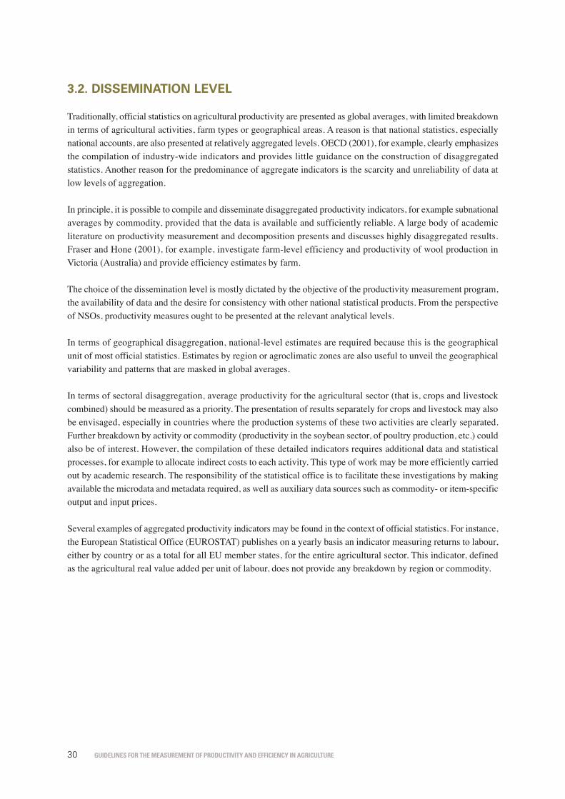
Guidelines for the measurement of productivity and efficiency in aGriculture30
3.2. dIssemInAtIon level
Traditionally, official statistics on agricultural productivity are presented as global averages, with limited breakdown in terms of agricultural activities, farm types or geographical areas. A reason is that national statistics, especially national accounts, are also presented at relatively aggregated levels. OECD (2001), for example, clearly emphasizes the compilation of industry-wide indicators and provides little guidance on the construction of disaggregated statistics. Another reason for the predominance of aggregate indicators is the scarcity and unreliability of data at low levels of aggregation.
In principle, it is possible to compile and disseminate disaggregated productivity indicators, for example subnational averages by commodity, provided that the data is available and sufficiently reliable. A large body of academic literature on productivity measurement and decomposition presents and discusses highly disaggregated results. Fraser and Hone (2001), for example, investigate farm-level efficiency and productivity of wool production in Victoria (Australia) and provide efficiency estimates by farm.
The choice of the dissemination level is mostly dictated by the objective of the productivity measurement program, the availability of data and the desire for consistency with other national statistical products. From the perspective of NSOs, productivity measures ought to be presented at the relevant analytical levels.
In terms of geographical disaggregation, national-level estimates are required because this is the geographical unit of most official statistics. Estimates by region or agroclimatic zones are also useful to unveil the geographical variability and patterns that are masked in global averages.
In terms of sectoral disaggregation, average productivity for the agricultural sector (that is, crops and livestock combined) should be measured as a priority. The presentation of results separately for crops and livestock may also be envisaged, especially in countries where the production systems of these two activities are clearly separated. Further breakdown by activity or commodity (productivity in the soybean sector, of poultry production, etc.) could also be of interest. However, the compilation of these detailed indicators requires additional data and statistical processes, for example to allocate indirect costs to each activity. This type of work may be more efficiently carried out by academic research. The responsibility of the statistical office is to facilitate these investigations by making available the microdata and metadata required, as well as auxiliary data sources such as commodity- or item-specific output and input prices.
Several examples of aggregated productivity indicators may be found in the context of official statistics. For instance, the European Statistical Office (EUROSTAT) publishes on a yearly basis an indicator measuring returns to labour, either by country or as a total for all EU member states, for the entire agricultural sector. This indicator, defined as the agricultural real value added per unit of labour, does not provide any breakdown by region or commodity.

Guidelines for the measurement of productivity and efficiency in aGriculture 31
3.3. From the BAsIC dAtA to the IndICAtor: the AggregAtIon proCedure
The aggregation procedure describes how the basic data is compiled to obtain the indicator at the targeted level of aggregation. In agricultural statistics, the elementary data collection unit is typically the agricultural holding or household. Aggregate productivity indicators can be compiled in two ways: (i) by summing and valuing farm-level outputs and inputs, or (ii) by calculating a weighted average of the farm-level productivity indicators. In theory, the choice of one procedure or the other should not modify the result, as argued in box 6.
In practice, the compilation of productivity indicators by statistical organizations is based on the separate aggregation of output or value added (numerator) and inputs (denominator), rather than from the averaging of farm-level productivity indices. Indeed, the former procedure is better able to cope with the diversity of data sources needed for productivity measurement, to respond to the objective of producing a countrywide measure and to ensure consistency over time.
A wide variety of data sources and actorsIn practice, the calculation of productivity is not solely based on a single data source, even if a comprehensive and well-structured farm survey conducted at regular intervals is available. Rather, data from a wide variety of sources are combined, each possibly with different scopes, reference periods and sectoral and geographical disaggregations.
A variety of organizations and government departments may be involved in the collection of basic data that may be of use in productivity measurement: information on production and inputs may be drawn from the main agricultural survey managed by the ministry of agriculture; data on labour may be collected within household or labour surveys, often managed by the NSOs; information on agricultural assets or inputs may originate from specialized business surveys; market prices for outputs and inputs may be obtained from market surveys, etc. Figure 5 illustrates the variety of the possible sources of data and their linkages to the different components of agricultural productivity. While not exhaustive, this list includes the major data sources typically used and available at country level. Given this variety of the sources of information, statistics on productivity, as most of the major economic indicators, are more easily calculated using precompiled and aggregated data on production, average prices or deflators, industry-level data on the receipts from the selling of agricultural inputs, etc.
Box 6. InvArIAnCe oF the IndICAtors to the AggregAtIon proCedure.
Let us assume that data is collected on outputs, inputs and their respective selling and purchase prices at the farm gate, allowing for the calculation of the value added and the cost of the factors of production for each farm. For each farm i, the returns to factors of production are:
36
presents and discusses highly disaggregated results. Fraser and Hone (2001), for example, investigate farm-level efficiency and productivity of wool production in Victoria (Australia) and provide efficiency estimates by farm.
The choice of the dissemination level is mostly dictated by the objective of the productivity measurement program, the availability of data and the desire for consistency with other national statistical products. From the perspective of NSOs, productivity measures ought to be presented at the relevant analytical levels.
In terms of geographical disaggregation, national-level estimates are required because this is the geographical unit of most official statistics. Estimates by region or agroclimatic zones are also useful to unveil the geographical variability and patterns that are masked in global averages.
In terms of sectoral disaggregation, average productivity for the agricultural sector (that is, crops and livestock combined) should be measured as a priority. The presentation of results separately for crops and livestock may also be envisaged, especially in countries where the production systems of these two activities are clearly separated. Further breakdown by activity or commodity (productivity in the soybean sector, of poultry production, etc.) could also be of interest. However, the compilation of these detailed indicators requires additional data and statistical processes, for example to allocate indirect costs to each activity. This type of work may be more efficiently carried out by academic research. The responsibility of the statistical office is to facilitate these investigations by making available the microdata and metadata required, as well as auxiliary data sources such as commodity- or item-specific output and input prices.
Several examples of aggregated productivity indicators may be found in the context of official statistics. For instance, the European Statistical Office (EUROSTAT) publishes on a yearly basis an indicator measuring returns to labour, either by country or as a total for all EU member states, for the entire agricultural sector. This indicator, defined as the agricultural real value added per unit of labour, does not provide any breakdown by region or commodity.
3.4. From the basic data to the indicator: the aggregation procedure
The aggregation procedure describes how the basic data is compiled to obtain the indicator at the targeted level of aggregation. In agricultural statistics, the elementary data collection unit is typically the agricultural holding or household. Aggregate productivity indicators can be compiled in two ways: (i) by summing and valuing farm-level outputs and inputs, or (ii) by calculating a weighted average of the farm-level productivity indicators. In theory, the choice of one procedure or the other should not modify the result, as argued in box 6.
Box 6. Invariance of the indicators to the aggregation procedure.
Let us assume that data is collected on outputs, inputs and their respective selling and purchase prices at the farm gate, allowing for the calculation of the value added and the cost of the factors of production
for each farm. For each farm 𝑖𝑖, the returns to factors of production are: 𝑝𝑝𝑝𝑝7 =𝑉𝑉7
𝑋𝑋7D , where 𝑉𝑉7 is farm
𝑖𝑖’s value added and 𝑋𝑋7 the cost of the factors of production. Average returns to factors of production for a given group of farms can be calculated either by the ratio of the total value added to total costs of
factors of production, 𝑝𝑝𝑝𝑝 = ∑𝑉𝑉7∑𝑋𝑋7
G , or equivalently by the cost-weighted average of farm returns,
𝑝𝑝𝑝𝑝 = ∑ \]
∑\]
^]\]= ∑ \]
∑\]𝑝𝑝𝑝𝑝7.
where Vi is farm i’s value added and Xi the cost of the factors of production. Average returns to factors of production for a given group of farms can be calculated either by the ratio of the total value added to total costs of factors of production,
36
presents and discusses highly disaggregated results. Fraser and Hone (2001), for example, investigate farm-level efficiency and productivity of wool production in Victoria (Australia) and provide efficiency estimates by farm.
The choice of the dissemination level is mostly dictated by the objective of the productivity measurement program, the availability of data and the desire for consistency with other national statistical products. From the perspective of NSOs, productivity measures ought to be presented at the relevant analytical levels.
In terms of geographical disaggregation, national-level estimates are required because this is the geographical unit of most official statistics. Estimates by region or agroclimatic zones are also useful to unveil the geographical variability and patterns that are masked in global averages.
In terms of sectoral disaggregation, average productivity for the agricultural sector (that is, crops and livestock combined) should be measured as a priority. The presentation of results separately for crops and livestock may also be envisaged, especially in countries where the production systems of these two activities are clearly separated. Further breakdown by activity or commodity (productivity in the soybean sector, of poultry production, etc.) could also be of interest. However, the compilation of these detailed indicators requires additional data and statistical processes, for example to allocate indirect costs to each activity. This type of work may be more efficiently carried out by academic research. The responsibility of the statistical office is to facilitate these investigations by making available the microdata and metadata required, as well as auxiliary data sources such as commodity- or item-specific output and input prices.
Several examples of aggregated productivity indicators may be found in the context of official statistics. For instance, the European Statistical Office (EUROSTAT) publishes on a yearly basis an indicator measuring returns to labour, either by country or as a total for all EU member states, for the entire agricultural sector. This indicator, defined as the agricultural real value added per unit of labour, does not provide any breakdown by region or commodity.
3.4. From the basic data to the indicator: the aggregation procedure
The aggregation procedure describes how the basic data is compiled to obtain the indicator at the targeted level of aggregation. In agricultural statistics, the elementary data collection unit is typically the agricultural holding or household. Aggregate productivity indicators can be compiled in two ways: (i) by summing and valuing farm-level outputs and inputs, or (ii) by calculating a weighted average of the farm-level productivity indicators. In theory, the choice of one procedure or the other should not modify the result, as argued in box 6.
Box 6. Invariance of the indicators to the aggregation procedure.
Let us assume that data is collected on outputs, inputs and their respective selling and purchase prices at the farm gate, allowing for the calculation of the value added and the cost of the factors of production
for each farm. For each farm 𝑖𝑖, the returns to factors of production are: 𝑝𝑝𝑝𝑝7 =𝑉𝑉7
𝑋𝑋7D , where 𝑉𝑉7 is farm
𝑖𝑖’s value added and 𝑋𝑋7 the cost of the factors of production. Average returns to factors of production for a given group of farms can be calculated either by the ratio of the total value added to total costs of
factors of production, 𝑝𝑝𝑝𝑝 = ∑𝑉𝑉7∑𝑋𝑋7
G , or equivalently by the cost-weighted average of farm returns,
𝑝𝑝𝑝𝑝 = ∑ \]
∑\]
^]\]= ∑ \]
∑\]𝑝𝑝𝑝𝑝7.
or equivalently by the cost-weighted average of farm returns,
36
presents and discusses highly disaggregated results. Fraser and Hone (2001), for example, investigate farm-level efficiency and productivity of wool production in Victoria (Australia) and provide efficiency estimates by farm.
The choice of the dissemination level is mostly dictated by the objective of the productivity measurement program, the availability of data and the desire for consistency with other national statistical products. From the perspective of NSOs, productivity measures ought to be presented at the relevant analytical levels.
In terms of geographical disaggregation, national-level estimates are required because this is the geographical unit of most official statistics. Estimates by region or agroclimatic zones are also useful to unveil the geographical variability and patterns that are masked in global averages.
In terms of sectoral disaggregation, average productivity for the agricultural sector (that is, crops and livestock combined) should be measured as a priority. The presentation of results separately for crops and livestock may also be envisaged, especially in countries where the production systems of these two activities are clearly separated. Further breakdown by activity or commodity (productivity in the soybean sector, of poultry production, etc.) could also be of interest. However, the compilation of these detailed indicators requires additional data and statistical processes, for example to allocate indirect costs to each activity. This type of work may be more efficiently carried out by academic research. The responsibility of the statistical office is to facilitate these investigations by making available the microdata and metadata required, as well as auxiliary data sources such as commodity- or item-specific output and input prices.
Several examples of aggregated productivity indicators may be found in the context of official statistics. For instance, the European Statistical Office (EUROSTAT) publishes on a yearly basis an indicator measuring returns to labour, either by country or as a total for all EU member states, for the entire agricultural sector. This indicator, defined as the agricultural real value added per unit of labour, does not provide any breakdown by region or commodity.
3.4. From the basic data to the indicator: the aggregation procedure
The aggregation procedure describes how the basic data is compiled to obtain the indicator at the targeted level of aggregation. In agricultural statistics, the elementary data collection unit is typically the agricultural holding or household. Aggregate productivity indicators can be compiled in two ways: (i) by summing and valuing farm-level outputs and inputs, or (ii) by calculating a weighted average of the farm-level productivity indicators. In theory, the choice of one procedure or the other should not modify the result, as argued in box 6.
Box 6. Invariance of the indicators to the aggregation procedure.
Let us assume that data is collected on outputs, inputs and their respective selling and purchase prices at the farm gate, allowing for the calculation of the value added and the cost of the factors of production
for each farm. For each farm 𝑖𝑖, the returns to factors of production are: 𝑝𝑝𝑝𝑝7 =𝑉𝑉7
𝑋𝑋7D , where 𝑉𝑉7 is farm
𝑖𝑖’s value added and 𝑋𝑋7 the cost of the factors of production. Average returns to factors of production for a given group of farms can be calculated either by the ratio of the total value added to total costs of
factors of production, 𝑝𝑝𝑝𝑝 = ∑𝑉𝑉7∑𝑋𝑋7
G , or equivalently by the cost-weighted average of farm returns,
𝑝𝑝𝑝𝑝 = ∑ \]
∑\]
^]\]= ∑ \]
∑\]𝑝𝑝𝑝𝑝7.
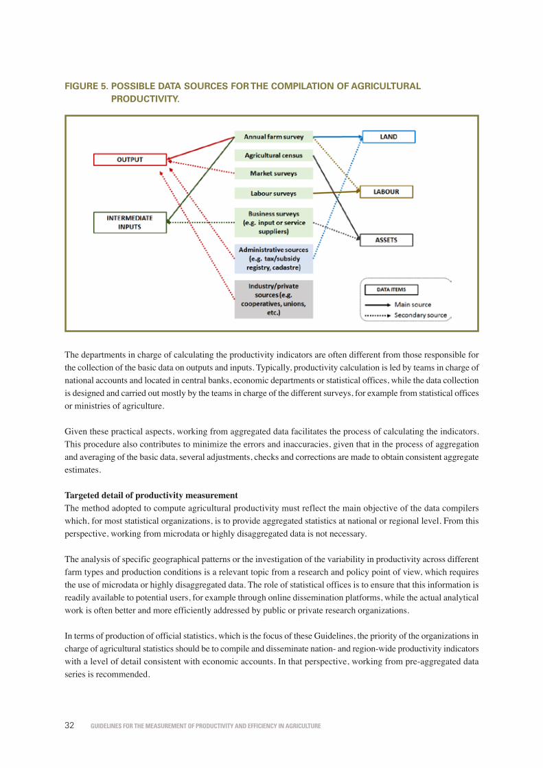
Guidelines for the measurement of productivity and efficiency in aGriculture32
FIgure 5. possIBle dAtA sourCes For the CompIlAtIon oF AgrICulturAl produCtIvIty.
The departments in charge of calculating the productivity indicators are often different from those responsible for the collection of the basic data on outputs and inputs. Typically, productivity calculation is led by teams in charge of national accounts and located in central banks, economic departments or statistical offices, while the data collection is designed and carried out mostly by the teams in charge of the different surveys, for example from statistical offices or ministries of agriculture.
Given these practical aspects, working from aggregated data facilitates the process of calculating the indicators. This procedure also contributes to minimize the errors and inaccuracies, given that in the process of aggregation and averaging of the basic data, several adjustments, checks and corrections are made to obtain consistent aggregate estimates.
Targeted detail of productivity measurementThe method adopted to compute agricultural productivity must reflect the main objective of the data compilers which, for most statistical organizations, is to provide aggregated statistics at national or regional level. From this perspective, working from microdata or highly disaggregated data is not necessary.
The analysis of specific geographical patterns or the investigation of the variability in productivity across different farm types and production conditions is a relevant topic from a research and policy point of view, which requires the use of microdata or highly disaggregated data. The role of statistical offices is to ensure that this information is readily available to potential users, for example through online dissemination platforms, while the actual analytical work is often better and more efficiently addressed by public or private research organizations.
In terms of production of official statistics, which is the focus of these Guidelines, the priority of the organizations in charge of agricultural statistics should be to compile and disseminate nation- and region-wide productivity indicators with a level of detail consistent with economic accounts. In that perspective, working from pre-aggregated data series is recommended.
37
In practice, the compilation of productivity indicators by statistical organizations is based on the separate aggregation of output or value added (numerator) and inputs (denominator), rather than from the averaging of farm-level productivity indices. Indeed, the former procedure is better able to cope with the diversity of data sources needed for productivity measurement, to respond to the objective of producing a countrywide measure and to ensure consistency over time.
A wide variety of data sources and actors In practice, the calculation of productivity is not solely based on a single data source, even if a comprehensive and well-structured farm survey conducted at regular intervals is available. Rather, data from a wide variety of sources are combined, each possibly with different scopes, reference periods and sectoral and geographical disaggregations.
A variety of organizations and government departments may be involved in the collection of basic data that may be of use in productivity measurement: information on production and inputs may be drawn from the main agricultural survey managed by the ministry of agriculture; data on labour may be collected within household or labour surveys, often managed by the NSOs; information on agricultural assets or inputs may originate from specialized business surveys; market prices for outputs and inputs may be obtained from market surveys, etc. Figure 5 illustrates the variety of the possible sources of data and their linkages to the different components of agricultural productivity. While not exhaustive, this list includes the major data sources typically used and available at country level. Given this variety of the sources of information, statistics on productivity, as most of the major economic indicators, are more easily calculated using precompiled and aggregated data on production, average prices or deflators, industry-level data on the receipts from the selling of agricultural inputs, etc.
Figure 5. Possible data sources for the compilation of agricultural productivity.
The departments in charge of calculating the productivity indicators are often different from those responsible for the collection of the basic data on outputs and inputs. Typically, productivity calculation is led by teams in charge of national accounts and located in central banks, economic departments or statistical offices, while the data collection is designed and carried out mostly by the teams in charge of the different surveys, for example from statistical offices or ministries of agriculture.
Given these practical aspects, working from aggregated data facilitates the process of calculating the indicators. This procedure also contributes to minimize the errors and inaccuracies, given that

Guidelines for the measurement of productivity and efficiency in aGriculture 33
Consistency over timeWorking from aggregated data also contributes to ensure consistency over time of the indicators. Indeed, properly measuring productivity growth rates and trends require that the basic data be collected and compiled in a consistent manner year after year. This means using the same geographical and sectoral scope, as well as data collection procedures that respect a common set of concepts, definitions and classifications.
When working directly from microdata, these conditions can only be fully fulfilled with panel surveys that follow the same sample of farms year after year, over a certain period. This is the approach taken by Fraser and Hone (2001), for example, to measure and analyse changes in productivity and efficiency over time. However, maintaining a panel is generally costly and operationally complex, in part because the units that drop out of the sample each year must be replaced by new units with similar characteristics, a process that may require the use of complex statistical procedures. Panel surveys are also known to impose a higher burden on respondents because the same units (farms) are visited several times over the survey period. Consistent average estimates can also be obtained from annual agricultural surveys with fresh samples taken every year, provided that the sample size is large enough and that there is no major change in the stratification and sampling procedure from one year to another. In any case, adjustments are always required.
Working from aggregated data limits the risk of bias associated with changes in scope, concepts and definitions over time. Indeed, aggregated data is often adjusted, corrected and validated to ensure that the final indicators form consistent time series. For example, in cases of changes to the scope of the data collection, such as the lowering of the size threshold below which farms are excluded from the sample survey or the adoption of a new classification system, the data series are adjusted backwards (“retropolated”, in technical jargon) to enforce the consistency of the time series.
3.4. levels And growth rAtes
Productivity indicators can be presented in terms of levels or growth rates, depending on the desired indicator (single-factor productivity, MFP or TFP) and the targeted disaggregation level.

Guidelines for the measurement of productivity and efficiency in aGriculture34
3.4.1. levelsIndicators in levels are expressed in the unit of the denominator of the productivity ratio. For the indicator to be meaningful, it should be possible to interpret the unit clearly. For example, partial productivity indicators are often easy to interpret because they are expressed in units, to which it is easy to relate. Indicators such as crop output by hectare or by person employed on the farm, for example, may be interpreted directly and unequivocally. Differences in levels can be compared across time, farm types, and countries. In principle, levels can be calculated for any stage of aggregation, from the farm to the sector.
Levels are also better adapted to the comparison of productivity across countries or farm types characterized by different levels of development or sophistication of agricultural production: output per worker, for example, can be directly compared across countries, and differences in the levels of this partial productivity indicator can be interpreted as differences in efficiency. Instead, the interpretation and comparison of growth rates may be affected by structural differences in stages of development. For example, the rate of increase in productivity tends to be lower in more sophisticated agricultural systems, which present high levels of productivity, because the best technologies are used and most of the technical efficiency gains may have already been exploited. On the contrary, growth rates are typically higher in developing countries, where agricultural remains largely traditional and with low levels of productivity, yet with largely untapped sources of efficiency and technological gains.
The agricultural TFP estimates released by the USDA-ERS International Agricultural Productivity (IAP) confirm this intuition: productivity growth in developing regions such as Latin America (including the Caribbean) and Asia has been higher than in North America and Europe, two regions with sophisticated input-intensive agricultural systems (figure 6). Sub-Saharan Africa is lagging in terms of productivity growth, reflecting the predominance of traditional farming and the much slower pace of transition towards more sophisticated and commercial farming activities for reasons, such as difficulty in accessing good-quality inputs, poor infrastructure, conflicts, etc., that will not be explored in detail here.
FIgure 6. AgrICulture tFp ChAnge, By regIon (2001–2014).
Source: Authors, based on data from USDA-ERS IAP1
1 https://www.ers.usda.gov/data-products/international-agricultural-productivity (updated on 16 October 2017).

Guidelines for the measurement of productivity and efficiency in aGriculture 35
3.4.2. growth ratesLevel indicators are not easy to interpret when they refer to multiple outputs and inputs: an indicator of the type “USD produced per USD spent on factors of production” is not as directly interpretable as “tons of wheat per planted acre”, for example. This is why analysis of aggregate agricultural productivity is often based on growth rates. Using growth rates also helps to mitigate measurement errors affecting levels, to the extent that these errors are stable in time.
The measurement of average growth rates is typically done through the construction of indices that describe the evolution in time of productivity in a meaningful and consistent way. The construction of indices to measure productivity change is a complex but well-researched topic. OECD (2001, pp. 83–92) offers a detailed discussion of index theory in relation to productivity measurement.
3.5. ChoosIng From A vArIety oF produCtIvIty IndICAtors
Chapter 2 briefly described the different types of productivity indicators, such as single-factor productivity and TFP. This section provides further details on the array of possible indicators, their uses, interpretation and challenges associated with their compilation. Examples of indicators from different countries are presented. Possible metrics range from single-output single-factor measures to TFP-like indicators combining bundles of outputs and inputs, with semi-aggregated and partial indicators in between (figure 7). The data requirements generally increase with the level of aggregation.
FIgure 7. From sIngle-FACtor produCtIvIty to tFp: InCreAsIng dAtA reQuIrements.
41
measures to TFP-like indicators combining bundles of outputs and inputs, with semi-aggregated and partial indicators in between (figure 7). The data requirements generally increase with the level of aggregation.
Figure 7. From single-factor productivity to TFP: increasing data requirements.
3.9. Single output and single input Definition and description
This is the most elementary form of productivity measure. This indicator measures the amount of output of a given commodity per unit of input (intermediate input or factor of production).
Both the output and the input are often expressed in physical units, as no commodity or input-wise aggregation is required. This indicator is adapted for a presentation in levels as: (i) the units in which outputs (quantities or values) and inputs (man-days, hectares of planted land, etc.) are expressed allow for direct interpretation; (ii) the use of physical units and the fact that only one output and input are considered facilitate the direct interpretation of productivity levels. Calculated in this way, this indicator is often referred to as physical productivity (tons of cereals produced out of one hectare of land, etc.).
Growth rates can be directly calculated from the quantity data to measure the change in the quantities of commodities produced per unit of input. Outputs or inputs can also be expressed in monetary values; however, in this case, the indicator loses its characteristic of physical metric.
Examples
Typical examples are crop yields, an indicator of land productivity that measures the quantity of commodity produced from a given area unit: tons of shelled maize per planted acre, kilograms of paddy per harvested hectare, etc. For crops, other examples include labour productivity, such as quantities of commodity produced per employed worker or per family member active on the farm. Similar indicators can be calculated for livestock products: litres of milk per milking cow, litres of milk per worker (labour productivity), etc. Crop yields and labour productivity being among the key indicators used to monitor the performance of the agricultural sector, they are compiled in most agricultural surveys and statistical programs in agriculture.
The Productivity Assessment Survey of Different Crops of Bangladesh, conducted by the Bureau of Statistics, provides an example of single-input single-output productivity measurement at

Guidelines for the measurement of productivity and efficiency in aGriculture36
3.5.1. single output and single input Definition and descriptionThis is the most elementary form of productivity measure. This indicator measures the amount of output of a given commodity per unit of input (intermediate input or factor of production).
Both the output and the input are often expressed in physical units, as no commodity or input-wise aggregation is required. This indicator is adapted for a presentation in levels as: (i) the units in which outputs (quantities or values) and inputs (man-days, hectares of planted land, etc.) are expressed allow for direct interpretation; (ii) the use of physical units and the fact that only one output and input are considered facilitate the direct interpretation of productivity levels. Calculated in this way, this indicator is often referred to as physical productivity (tons of cereals produced out of one hectare of land, etc.).
Growth rates can be directly calculated from the quantity data to measure the change in the quantities of commodities produced per unit of input. Outputs or inputs can also be expressed in monetary values; however, in this case, the indicator loses its characteristic of physical metric.
ExamplesTypical examples are crop yields, an indicator of land productivity that measures the quantity of commodity produced from a given area unit: tons of shelled maize per planted acre, kilograms of paddy per harvested hectare, etc. For crops, other examples include labour productivity, such as quantities of commodity produced per employed worker or per family member active on the farm. Similar indicators can be calculated for livestock products: litres of milk per milking cow, litres of milk per worker (labour productivity), etc. Crop yields and labour productivity being among the key indicators used to monitor the performance of the agricultural sector, they are compiled in most agricultural surveys and statistical programs in agriculture.
The Productivity Assessment Survey of Different Crops of Bangladesh, conducted by the Bureau of Statistics, provides an example of single-input single-output productivity measurement at national level. The stated objectives of this program are to measure per-acre production costs, yields, production value and area under cultivation, for different crops. The crops (ginger, pineapple, pumpkin, banana, etc.) are surveyed periodically and in rotation.2 The concept of productivity used is relatively narrow, as it is restricted to a single input (land) and a single output (the commodity). These surveys also collect and compile data on production value and costs that can be used to measure the value added as well as the returns to labour. These types of surveys constitute key sources of information from which to compile economic accounts for agriculture and aggregate sector-level productivity.
A numerical example of returns to specific factors of production for individual commodities is shown in figure 8, which displays returns to labour in the corn industry in the United States of America. The value-added (calculated as the production value minus operating costs) in terms of USD generated by spending 1 USD on labour (hired and family) is estimated at USD 9 for the entire country, although with significant variations across regions (USD 6 to 11).
2 Bangladesh. Ministry of Planning. Bangladesh Bureau of Statistics. 2015. Report on the Productivity Survey of Ginger Crop. Productivity Assessment Survey of Different Crops Programme. (other commodity reports are also available).

Guidelines for the measurement of productivity and efficiency in aGriculture 37
FIgure 8. return to lABour For Corn produCtIon In the usA (By regIon, 2016).
Source: Authors, based on data from ERS/ARMS (USDA)
Data requirementsCrops. To compute single-output single-factor productivity indicators, data is required at least on outputs and inputs in terms of quantity or physical units. Typically, this data would come from farm surveys, which collect information on variables such as planted area, quantities harvested for crops and the amounts of labour and capital used.
If output is measured using the value-added concept, data on the intermediate inputs should also be captured. As intermediate inputs must be aggregated and the resulting amount deducted from the gross output measure, common units must be used. Prices for intermediate inputs and output prices are therefore required.
Livestock. Information is necessary on the number of heads by animal and on the output for the different livestock products, expressed in appropriate units: weight of animals sold for slaughter, litres of milk produced, tons of skins, etc. Depending on the input considered for productivity assessment, information may be required on feed, labour and capital used for livestock.
Commodity-specific data. The compilation of productivity indicators by commodity requires that data on factors of production and intermediate inputs be collected for each individual commodity. This might be difficult given that many inputs are shared across different commodities. For example, the same worker may be involved in both cropping and livestock activities, and quantifying the time spent separately on each activity is not straightforward; a given pesticide may be purchased and used for different crops; similar feed may be given to different animals (such as milking cows and cattle raised for slaughter); farm vehicles or machinery may be used to transport different commodities. In addition, most overhead costs such as water, electricity or fuel are typically asked at the farm level and not by commodity.
usd
Guidelines for the measurement of productivity and efficiency in aGriculture38
The compilation of single-output indicators therefore requires some degree of allocation of common costs to individual commodities, based on allocation keys such as planted area, production quantities or number of heads. The allocation process may require excessive simplification and approximation, thus undermining the overall accuracy of the results. Global Strategy (2016) provides an overview of the possible allocation methods, which vary depending on the commodity considered and the input to be allocated. Lips (2017) presents a model-based approach to allocate indirect farm-level costs to the different commodities using prior information and assumptions on technical coefficients (ratio of inputs to production, area or number of heads, depending on the situation).
3.5.2. multiple outputs and single input Definition and descriptionThis indicator measures, for a bundle of commodities, the amount of aggregate output produced per unit of input. At farm level, for instance, the productivity of labour, land or capital can be measured for all the commodities produced by the farm or a subset thereof (for example, only crop output) and not for a single commodity, as in the case of the single-output single-input statistic.
Measuring productivity for a set of commodities provides an indication on the performance of the wider farming sector. Indeed, the commodity mix (of a farm or, by extension, of a region or country) is to some extent the result of agronomic optimization and economic maximization: the farmer aims to maximize total yield, production and income, given the production conditions under which the farm is operating (climate, soil fertility, access to inputs, etc.). The choice of crops or activities depends, to some extent at least, on these parameters and their evolution. The assessment of the economic performance of farming systems through productivity analysis is conducted optimally by studying the entire system (in other words, a sufficiently large set of commodities produced) rather than by isolating a single activity, even if it is considered the major one.
For example, the practice of rotating crops on a field is often used to maximize the yield of a leading crop: the planting of a leguminous crop, for instance, helps to fix nitrogen in the soil, to the benefit of a subsequently grown crop (usually a cereal). In addition, the practice of crop rotation also helps to reduce pest and weed infestation and therefore contributes to maximize yields and reduce costs (for example, relating to pesticides and herbicides). In addition to yield maximization, crop rotations also contribute to diversify the commodity mix of the farm, reducing its exposure to risks (regarding market or price, climate, etc.) and improving its capacity to exploit market opportunities. The combination of crop production with the rearing of livestock can also be viewed as an integrated system, as crops or crop residues (fodder crops, hay, etc.) can be used as input (feed) for the livestock production. The measurement of productivity for groups of commodities therefore makes agronomic and economic sense, as it is more closely linked to the generation of income.
The calculation process requires that the production of the different commodities be aggregated into a single measure of output. This is typically done by aggregating the respective monetary equivalent, or value, of the output of each commodity. If the commodities considered belong to the same group, such as cereals or root crops, the output can be expressed in physical units (kg, tons, etc.); however, if the commodities are of different natures, such as cereals and root crops, or meat and milk, their output should be converted to a common unit to be aggregated. To facilitate comparability and ensure consistency across estimates, these Guidelines recommend using producer prices (farm-gate prices) to value the output of the different commodities.
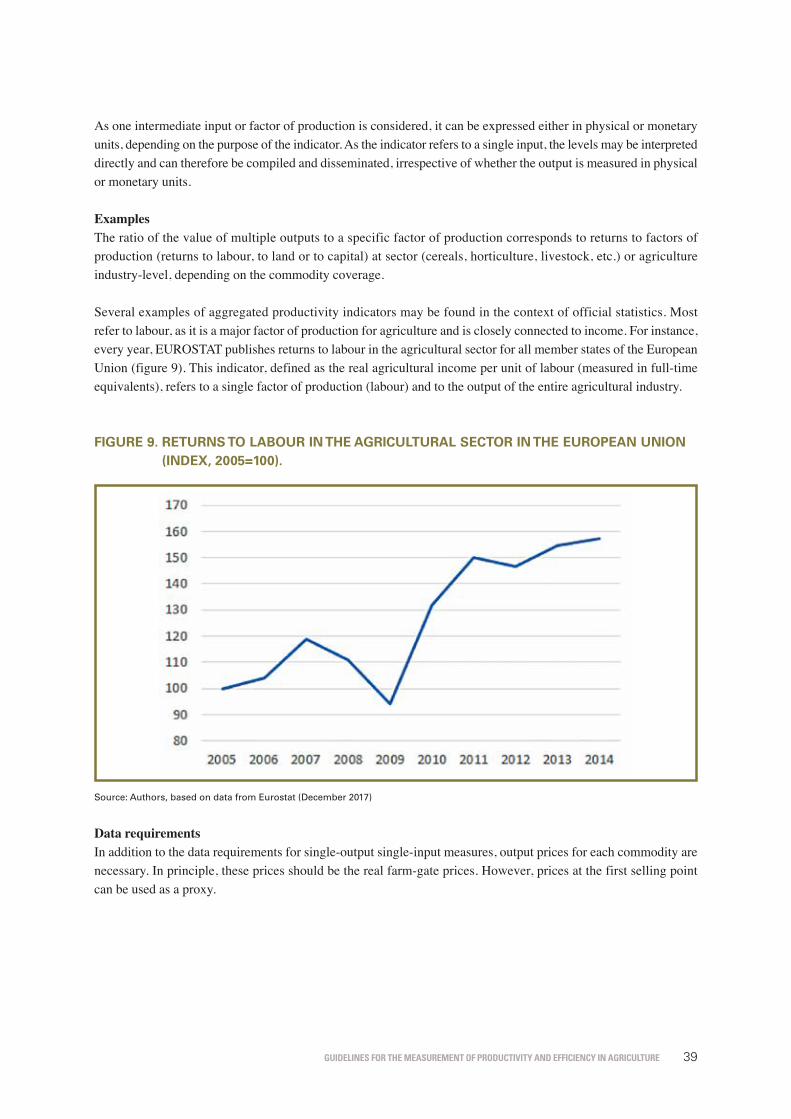
Guidelines for the measurement of productivity and efficiency in aGriculture 39
As one intermediate input or factor of production is considered, it can be expressed either in physical or monetary units, depending on the purpose of the indicator. As the indicator refers to a single input, the levels may be interpreted directly and can therefore be compiled and disseminated, irrespective of whether the output is measured in physical or monetary units.
ExamplesThe ratio of the value of multiple outputs to a specific factor of production corresponds to returns to factors of production (returns to labour, to land or to capital) at sector (cereals, horticulture, livestock, etc.) or agriculture industry-level, depending on the commodity coverage.
Several examples of aggregated productivity indicators may be found in the context of official statistics. Most refer to labour, as it is a major factor of production for agriculture and is closely connected to income. For instance, every year, EUROSTAT publishes returns to labour in the agricultural sector for all member states of the European Union (figure 9). This indicator, defined as the real agricultural income per unit of labour (measured in full-time equivalents), refers to a single factor of production (labour) and to the output of the entire agricultural industry.
FIgure 9. returns to lABour In the AgrICulturAl seCtor In the europeAn unIon (Index, 2005=100).
Source: Authors, based on data from Eurostat (December 2017)
Data requirementsIn addition to the data requirements for single-output single-input measures, output prices for each commodity are necessary. In principle, these prices should be the real farm-gate prices. However, prices at the first selling point can be used as a proxy.

Guidelines for the measurement of productivity and efficiency in aGriculture40
3.5.3. single output and multiple inputs Definition and descriptionThis indicator measures the productivity of a commodity with respect to the bundle of inputs used in its production. It has been discussed above that assessing the productivity of a bundle of commodities often makes more economic sense from the point of view of farming activities, given the multiple commodities generally produced by agricultural holdings and the linkages between them, particularly in developing countries. However, when a crop is mostly grown independently from others in intensive monoculture systems, a commodity-specific measure of productivity is also relevant.
Depending on the approach chosen, the numerator of this ratio can be either the gross output or the value added (gross output minus intermediate consumption). When gross output is used, the denominator comprises both intermediate inputs and factors of production. When the value added is used, the denominator only comprises factors of production.
The different inputs are aggregated by converting the quantities used (kg of fertilizers, man-days of labour, etc.) into their monetary equivalents. As the output refers to a single commodity, it can be expressed in either physical or monetary units. To ensure consistency with the denominator, it is however recommended to express the output in value terms.
This indicator can be expressed either in levels or in growth rates. The ratio of the value added to the factors of production provides a direct measure of the combined returns to labour, land and capital (USD amount of value added by spending 1 USD on factors of production).
ExamplesThe Commodity Costs and Returns program of the USDA/ERS disseminates data on output and inputs by commodity. From this data, several indicators can be calculated, including returns to factors of production. An illustration for milk production is shown in table 1. As the data is expressed in terms of current prices, the evolution of the indicator cannot be interpreted as changes in the productivity of the factors of production: indeed, changes in the indicator may also result from changes in prices (of outputs and inputs) and therefore may not fully reflect quantity or volume changes. The numerator (A) and denominator (B) should be deflated by appropriate price indices to construct a factor productivity series. The indicator in current prices can be interpreted as the returns to factors of production for a given year.
tABle 1. returns to FACtors oF produCtIon For mIlk In the usA.
dollars per hundredweight (cwt) of milk sold 2010 2011 2012 2013 2014 2015 2016
Value of production less operating costs (A) 4,96 5,86 3,81 2,30 6,65 1,42 0,87
Factors of production (B) 6,95 6,96 7,22 7,39 7,56 7,73 7,83
• Hired labor 1,46 1,49 1,54 1,58 1,61 1,69 1,75
• Opportunity cost of unpaid labor 2,19 2,11 2,16 2,22 2,25 2,28 2,31
• Capital recovery of machinery and equipment 3,28 3,34 3,50 3,57 3,68 3,73 3,75
• Opportunity cost of land (rental rate) 0,02 0,02 0,02 0,02 0,02 0,02 0,02
returns to factors of production (A/B) 0,71 0,84 0,53 0,31 0,88 0,18 0,11
Source: Authors, based on data from USDA/ERS (Dec. 2017)

Guidelines for the measurement of productivity and efficiency in aGriculture 41
Data requirementsTo construct a single-output and multiple-inputs indicator such as the returns to factors of production presented above, data is needed on: the quantities of output for the commodity and its producer price; the quantities of intermediate inputs and the respective purchase prices; and the quantities of factors of production used with their respective price or cost. Obtaining separate quantity and price data is ideal as this facilitates the construction of the volume measure of output (or value added) and inputs. However, when working with aggregated data, information is often available only in terms of values, the prices being available separately in the form of indices or deflators. In this situation, the productivity indicator can be compiled directly from the series in values, deflated by the appropriate price indices or deflators.
3.5.4. multiple outputs and multiple inputs Definition and descriptionThis indicator has been referred to in these Guidelines as TFP or MFP. Calculated as the ratio of total output to total inputs (both expressed in terms of volume), this indicator measures the overall efficiency or performance of production.
In principle, TFP can be calculated at any level of aggregation, from the farm to the aggregate industry level. For a farm, this indicator captures the efficiency of the overall production of the holding, combining all its activities and all of the inputs used in the various production processes. When calculated for the entire agricultural industry, this indicator measures the overall efficiency of agricultural production, combining all crops, livestock and other agricultural activities. TFP can also be broken down by sectors, such as crops and livestock, or by subsectors, such as annual crops, permanent crops and horticulture. When the value-added approach is used, TFP measures the returns to factors of production for the entire agricultural sector, or for a subset, if the indicator is broken down by commodity groups.
TFP or MFP indicators are typically expressed in growth rates, particularly when they are compiled at industry level. At farm level, if the gross output approach is used, this indicator is equivalent to net production margins.
Heterogeneous commodities or cost items are aggregated in the numerator and denominator using their monetary equivalents. A TFP indicator in levels is therefore expressed in monetary units. As noted above, other common units could be chosen in principle, if the common practice is to use monetary units. For the compilation of an aggregated measure of output, for example, the calorific content of each commodity could be a possible conversion unit.
ExamplesIndicators of total productivity or MFP in agriculture at country level are not commonplace. Indeed, few countries collect all of the data required to implement the standard growth accounting approach. Even in countries where most or part of the data is available, TFP indicators are scarce because of a lack of awareness on the relevant methodologies, particularly in developing countries with limited experience in economic statistics and national accounting. These Guidelines seek to bridge this methodological gap and to provide clarity on the type of data required for productivity measurement.
Examples of TFP measurement in agriculture are most often found in international organizations or in national departments in charge of compiling international statistics on agriculture. A reason for this is that such organizations often benefit from the availability of consistent international data sets that can be used for all sorts of modelling, estimations and imputations needed to measure productivity.
Productivity estimates also constitute an interesting basis for comparing production efficiency across countries and commodities, a topic of special interest for organizations involved in policy-making and analysis in the agricultural sector. An example of TFP measure has been presented above (figure 6), based on statistics from the USDA/ERS,

Guidelines for the measurement of productivity and efficiency in aGriculture42
to illustrate differences in TFP growth across different regions of the world. These TFP estimates, compiled using the growth accounting method, are one of the very few examples of productivity measures in agriculture to allow for consistent international comparisons. The estimates are disseminated as regional or subregional averages (for example, Southeast Asia), although not at country level.
The OECD has also compiled TFP indicators for the agricultural sector. These statistics are available for several of its member countries, with relatively long time series (from 1990 to 2009, for some countries). Figure 10 displays the year-on-year changes in MFP in the agricultural sector in Italy. In this case, the agricultural sector is taken in the broad sense, including crops, livestock, hunting, forestry and fishing. The MFP estimate for Italy shows a relatively high volatility and a distinctive downwards trend. The metadata provided by the OECD for this indicator shows that the MFP estimates follow the Solow residual approach and use cost shares. In other words, the measurement is based on the growth accounting approach, the change in productivity being the difference between output and input growth, with revenue and cost shares to weight commodities and inputs, respectively (as described in box 2). The agricultural value added is used in the numerator of the productivity ratio, with intermediate consumption deducted from the gross output.
FIgure 10. ChAnge In mFp In the AgrICulturAl seCtor (ItAly, In perCentAges).
Source: Authors, based on data from OECD Stat (January 2017)
Data requirementsTFP indicators are the most demanding in terms of data because they require information on all outputs, intermediated inputs and factors of production in quantity and value terms. The data requirements vary depending on the measurement approach. If the growth accounting method is used, as recommended by these Guidelines, information is required on quantities produced for each commodity and the inputs used (intermediate inputs and factors of production) throughout the period of analysis. To compute revenue and costs shares, data on the prices (selling, farm-gate or purchase) are required. The amount and detail of the information required on prices, which is more difficult to obtain than quantities, varies according to the weighting procedure: prices referring to the beginning of the period of analysis (Laspeyres index), to the end (Paasche index), to both (Fisher index) or continuously, over the entire period (Törnqvist index).
%
Guidelines for the measurement of productivity and efficiency in aGriculture 43
3.6. summAry oF reCommendAtIons
Box 7. summAry oF reCommendAtIons.
Aggregation• In terms of geographical breakdown, the construction of nation-wide productivity measures should be
prioritized. Breakdowns by regions or other areas can be compiled, provided that data is available and sufficiently reliable.
• In terms of commodity breakdown, the priority is to compile productivity measures for the entire agricultural sector (crops and livestock). Commodity or activity-specific information can also be compiled, contingent on data availability and quality.
• Additional breakdowns and analysis should be left to academic research.• The compilation of agricultural productivity at national or regional level is done efficiently by working from
pre-aggregated and validated data on outputs and inputs.
Levels versus growth rates• Growth rates are the preferred measure for multi-output multi-input productivity (TFP/MFP).• Levels can be used for partial or single-input indicators.• When making comparisons across groups with very different levels of agricultural development, the levels
can be disseminated, as they help to put growth rates into perspective (for example, high growth rates but from very low levels).
Productivity metrics• TFP or MFP measures should be the primary objective of a productivity program at country level.• These indicators can be complemented by partial metrics, to isolate the effect of individual inputs or to focus
the analysis on specific commodities.

Guidelines for the measurement of productivity and efficiency in aGriculture44
Guidelines for the measurement of productivity and efficiency in aGriculture 4545
Collecting data for productivity measurement4.1. IntroduCtIon And overvIew
The previous chapters presented the main definitions, the conceptual framework and the various operational approaches that may be adopted to measure productivity in agriculture. The objective of a productivity measurement program, the conceptual decisions regarding the boundaries of the indicators and the type and form of the metrics determine what data is needed and how to collect it.
In this respect, it is useful to recall the overall approach recommended by these Guidelines to measure TFP in agriculture, as being the difference between the revenue-weighted outputs and the cost-weighted inputs (Fuglie, 2015):
49
4 Collecting data for productivity
measurement
4.1. Introduction and overview
The previous chapters presented the main definitions, the conceptual framework and the various operational approaches that may be adopted to measure productivity in agriculture. The objective of a productivity measurement program, the conceptual decisions regarding the boundaries of the indicators and the type and form of the metrics determine what data is needed and how to collect it.
In this respect, it is useful to recall the overall approach recommended by these Guidelines to measure TFP in agriculture, as being the difference between the revenue-weighted outputs and the cost-weighted inputs (Fuglie, 2015):
𝑇𝑇𝑇𝑇𝑇𝑇) ≅ 𝑅𝑅7𝑌𝑌7,)
:
7;<
− 𝑆𝑆>𝑋𝑋>,)
?
>;<
[3]
where 𝑅𝑅7 is the share of commodity 𝑖𝑖 in total production value and 𝑆𝑆> is the share of intermediate input or factor of production 𝑗𝑗 in the total costs of production (see box 2 for more details). The minimal information requirements for agricultural productivity can be derived from this formula and are:
• A measure of the annual change in the volumes or quantities of agricultural outputs and inputs (𝑌𝑌7,) and 𝑋𝑋>,), respectively) over the period of analysis (𝑡𝑡 = 1, … , 𝑇𝑇);
• The prices and physical quantities of these outputs and inputs, for at least one year or period, so that the weights (𝑅𝑅7 and 𝑆𝑆>, respectively) can be determined.
In its simplest formulations, the measure of aggregate change can be based on Laspeyres or Paasche weights: the first period or year is used as the reference for Laspeyres, and the last for Paasche. More sophisticated weighing schemes, such as the Fisher or Törnqvist forms, require additional data on individual prices and quantities.
This chapter is intended to guide readers through the various steps of collection and compilation of the data required to measure productivity in a consistent manner and ensuring that the indicators display the desired properties. The various data items are described, and the data collection and compilation options are identified. The different options are assessed in terms of their respective precision, granularity level, cost and implications for the relevance and reliability of the productivity indicators. This chapter also links, on one hand, the type of and properties desired for the final indicators (TFP, single-factor indicator, etc.), and on the other, data needs, to help data compilers understand the implications (in terms of data requirements) of choosing productivity indicators with certain characteristics.
where Ri is the share of commodity i in total production value and Sj is the share of intermediate input or factor of production j in the total costs of production (see box 2 for more details). The minimal information requirements for agricultural productivity can be derived from this formula and are:• A measure of the annual change in the volumes or quantities of agricultural outputs and inputs (Yi,t and Xi,t,
respectively) over the period of analysis (t = 1,…,T);• The prices and physical quantities of these outputs and inputs, for at least one year or period, so that the weights
(Ri and Sj, respectively) can be determined.
In its simplest formulations, the measure of aggregate change can be based on Laspeyres or Paasche weights: the first period or year is used as the reference for Laspeyres, and the last for Paasche. More sophisticated weighing schemes, such as the Fisher or Törnqvist forms, require additional data on individual prices and quantities.
4

Guidelines for the measurement of productivity and efficiency in aGriculture46
This chapter is intended to guide readers through the various steps of collection and compilation of the data required to measure productivity in a consistent manner and ensuring that the indicators display the desired properties. The various data items are described, and the data collection and compilation options are identified. The different options are assessed in terms of their respective precision, granularity level, cost and implications for the relevance and reliability of the productivity indicators. This chapter also links, on one hand, the type of and properties desired for the final indicators (TFP, single-factor indicator, etc.), and on the other, data needs, to help data compilers understand the implications (in terms of data requirements) of choosing productivity indicators with certain characteristics.
This chapter covers the measurement of agricultural output, intermediate inputs and factors of production, for both cropping activities and livestock rearing.
As a preliminary remark concerning data sources and availability, it is important to note that, especially in developing countries, data collection systems are relatively well developed for the household sector, and less so for the institutional sector (that is, formally constituted farm holdings). The scope of the data collection should cover both sectors; however, the data availability and sources will likely differ. For example, large farm surveys may be available for the household sector, while data for the institutional sector may be obtained from industry sources, other secondary data providers (administrative data, etc.) or, more immediately, from business surveys. These characteristics should be borne in mind when identifying the data needs for the compilation of agricultural productivity, and the associated data sources.
4.2. AgrICulturAl output
4.2.1. measurement principlesProductivity is measured as a ratio of output to inputs. A proper assessment of agricultural output is therefore the starting point of any productivity program, whatever the measure chosen for the numerator of the productivity ratio (gross output or value added).
From a conceptual perspective, to keep measures of productivity consistent and aligned with economic theory, production should measure the total output resulting from a specific production process that combines intermediate inputs and factors of production to create a product. Output is counted if the product is used for home consumption by the agricultural household, sold for domestic final consumption, for export or added to inventories. Practices for the treatment of products that are used as an intermediate input for other agriculture products may vary; however, whatever method is chosen, this concept must be consistent on both the output and the input sides of the farm accounting balance sheets: if it is accounted for as output for one activity (such as production of fodder crops), it must be considered input for another enterprise (for example, feed for livestock).
From an operational point of view, measuring output for the purposes of productivity assessment involves collecting raw data on the physical quantities produced for several commodities and farm-gate prices (producer prices), or a proxy, to value production. This section describes the data collection and compilation issues for both crops and livestock.

Guidelines for the measurement of productivity and efficiency in aGriculture 47
4.2.2. Crops
QuantitiesThe production of the various crops should be covered as exhaustively as possible. Failure to account for a share of crop production, for example leaving aside secondary or relatively minor crops, inevitably leads to an underestimation of productivity.
An adequate assessment of crop production starts with a proper measurement of total harvested quantities. This variable, typically collected for each agricultural season, can be adjusted to the calendar year to ensure consistency with other statistics. Harvested quantities may be sold, consumed by the agricultural household, set aside as seeds for the next agricultural season, used as feed or added to stocks.
When measuring productivity, the objective is to assess the amount of produce that is effectively available for selling, consumption or use, as this is the amount that the farmer can count on for his livelihood. In other words, data compilers should capture production net of harvesting losses and, if possible, net of on-farm post-harvest losses. Reducing farm losses may result in higher productivity, if it leads to higher output at no or limited additional cost.1 The production to be captured (Q) is therefore given by:
Q = harvested quantities – on-farm losses
This is the output concept adopted in most countries and used to report production to FAO and other international organizations. Some countries apply loss parameters to harvested quantities to account for the losses occurring on the farm from the harvest to the storage or selling of the produce. However, information on post-harvest losses is typically scarce, especially in developing countries, and the loss parameters used are often outdated, highly uncertain or simply absent. The user may refer to the Guidelines on the measurement of harvest and post-harvest losses for guidance on how to collect and estimate losses for grain crops.2
To ensure consistency with the SNA framework, products transformed on the farm should not be included in crop output. The products to be considered must be raw commodities, which may have undergone some degree of transformation to reach the form in which they are sold or consumed. For example, while, after shelling or threshing and cleaning, maize grains are accounted for in crop production, the production of maize flour, even if carried out on the farm by the same agricultural holding or household, is not. Other examples include holdings producing wine or olive oil: the production to be recorded should only refer to quantities of grapes and olives, respectively. Transformed products can be accounted for in crop production when the inputs used to produce them cannot be separated from the other farm expenses or when the marketable or usable form of the commodity requires some transformation, such as in the case of fodder crops.
The methods to measure crop output will not be addressed in this document, as they go beyond its scope and because the estimation methods – for example those based on yield estimation through crop-cutting and assessment of planted or harvested area by crop – are now well established and used in most countries that conduct regular farm surveys.
1 In some situations, reducing losses is less economically interesting than inaction. For example, reducing the harvesting losses of certain fruit trees may require carrying out several fruit-picking operations, which would increase labour costs to an extent that outweighs the gains terms of yields. Overall, the economic benefit of reducing losses decreases with the level of percentage losses.
2 GSARS. 2018. Guidelines on the measurement of harvest and post-harvest losses. Global Strategy Guidelines: Rome.

Guidelines for the measurement of productivity and efficiency in aGriculture48
ValuesWhen measuring TFP, the output of different crops must be aggregated and value-weights must be constructed. This means that data on crop prices or, alternatively, directly on output values, must be collected.
Different prices can be used to value the output. They differ in the treatment of taxes and subsidies on the products, and the inclusion or exclusion of transport and trade margins. Output can be valued at basic price (producer’s price) or purchaser’s price. Details on the different prices are available in OECD (2001). In these Guidelines, it is recommended to use farm-gate prices to value output: in other words, the prices received by the farmer for his products. This price concept is also referred to as the basic price or producer’s price. Basic prices are net of any tax paid or subsidy received by the farmer. In other words, any tax (or subsidy) payable on the output is treated as if it were paid (or, as relevant, received) by the purchaser directly to (or from) the tax authority, instead of being an integral part of the price paid to the producer (OECD, 2001). In practice, producer’s prices are difficult to obtain, because they require farm-level information on the prices received. Prices at the first selling point, for example at wholesale or even retail markets, can be used as proxies. In principle, transport costs and margins should be deducted from the market prices to approach the true producer’s price.
In certain situations, prices may be difficult or even impossible to obtain. Indeed, markets for certain commodities may be thin or even inexistent, impeding the estimation of a representative selling price. In certain countries, for example, cereals such as millet or commodities used as inputs in other production process, for example as fodder crops for livestock feed, are often largely used for household consumption or for the intermediate consumption of the same holding. In these situations, there are often too few economic transactions to obtain solid information on prices.
While the prices collected refer to market transactions and concern the share of the output that is sold on the market3 by agricultural holdings, all output (referred to as Q above), including the amount consumed by the agricultural household, used by the holding or stored, should be valued. In practice, the selling prices by commodity obtained from market transactions can be used to value the unsold share of the output. Indeed, market prices can be considered as a good approximation of the opportunity cost of retaining the output.
4.2.3. livestock
QuantitiesBefore collecting data on output, the first step is to identify the different livestock products: for example, whether they are meat, milk, eggs or live animals. The output of each type of livestock product is measured in specific units, such as animal heads for live animals, tons for meat, thousands of litres for milk, etc. FAO (1999)4 and OECD (2002)5 provide an operational categorization of the different livestock products, from the perspective of the agricultural household:• Outputs that can be consumed only once: these products are mainly meat, milk and eggs • Products that can be used several times, either for consumption or as input for subsequent production activities,
such as animal skins, wool, etc.
3 Here, the term “market” is used in a broad sense, comprising any economic transaction, irrespective of the place where this transaction takes place (on the farm, at a cooperative, wholesale market, etc.) and the number of participants (sellers and buyers).
4 FAO. 1999. Regional Office of Asia and the Pacific. Poverty alleviation and food security in Asia: role of livestock. http://www.fao.org/docrep/003/x6627e/x6627e00.htm
5 OECD. 2002. Measuring the non-observed economy: a handbook. https://www.oecd.org/std/na/1963116.pdf

Guidelines for the measurement of productivity and efficiency in aGriculture 49
In addition to these two types of output, live animals should also be accounted for as a separate class of output. For the purposes of productivity measurement, these Guidelines recommend that measurement efforts be concentrated on those outputs that are of major importance for food security and farm income, typically live animals, meat, milk and eggs.
Similarly, the animal species to be covered in the measurement of output should reflect their respective importance for the countries’ livestock sector. In other words, minor species should be covered only if there is a specific need to collect data on these species, for instance because of their importance in certain localities or because of an anticipated growth in the market for these animals.
This section does not detail how livestock production should be measured, as this is a specialized topic that goes beyond the scope of productivity measurement strictly speaking and has already been addressed in several manuals and research papers. Interested readers may refer to the Guidelines on the measurement of livestock production, published by the Global Strategy in 2018, for an extensive presentation of these methods.
ValuesThe construction of productivity indicators for the livestock sector requires the determination of value weights to be applied to the quantity or volume changes in livestock output. Information on prices is therefore required: analogously to crops, the appropriate prices with which to value output are those received by the farmer (farm-gate or producer prices). Prices at the first point of sale of animals (such as the market) or animal products are an acceptable proxy.
As for crops, it is important to reiterate that the entire livestock production should be valued. In other words, the share of the output that does not reach the market (milk consumed by the agricultural household, animals slaughtered on the farm for own consumption, etc.) should also be valued, for example using the average or median prices obtained from the marketed output. Failure to do so would lead to an underestimation of livestock output and a possible underestimation of the productivity in the livestock sector.
4.3. IntermedIAte Inputs
Intermediate inputs are goods used in the production process of agricultural commodities and that are entirely (or mostly) used during the agricultural season or calendar year. For the purposes of agricultural productivity measurement, it is recommended to collect prices (or values) and quantity information for intermediate inputs, to calculate the cost shares of those inputs. This section presents the scope in terms of intermediate inputs and the characteristics of the data needed for productivity measurement.
4.3.1. For crops
QuantitiesFor crops, the major intermediate inputs include seeds, fertilizers, crop protection products (herbicides, insecticides, etc.), water used for irrigation, energy (fuel, electricity) as well as small tools and equipment used for specific activities (protection clothing, etc.).
Guidelines for the measurement of productivity and efficiency in aGriculture50
It is important to collect information on all these inputs, irrespective of their source of acquisition. Some of them may have been purchased from agrodealers or other providers; others may be self-supplied by the agricultural holding: seeds set aside from the previous harvest and organic fertilizers produced by the farm (in the form of manure, compost or other bio-fertilizers) are the most common examples. Self-supplied inputs may constitute a significant share of the intermediate inputs used by the holdings, especially in small farms of developing countries. Failure to account for these inputs would bias the estimate of input use downwards and therefore artificially inflate productivity, everything else equal.
Information on the amount of inputs used for cropping activities may be collected directly, from the farmer, or indirectly, through enquiries to input providers. As a general rule, the selling units can be used as references for data collection (20-kg bag of fertilizer, 10-litre can of insecticide, etc.) or, alternatively, any of the units commonly handled and known by the actors: kg, litres, bags, drums, tins and other containers of a certain volume or weight, for example. For analytical, aggregation and valuation purposes, the data collected in non-standard units should be converted to standard units (such as kg). Details on the collection and processing of data on input use and prices are provided in Global Strategy (2016).
ValuesExcept for the limited case of single-factor or single-input indicators, the quantities of the different intermediate inputs used in crop production must be valued and aggregated into a single input measure. This requires that the inputs be valued at the price effectively paid by the farmer to purchase them. Price information can be directly recorded from the purchases made by the farmer (usually collected in farm surveys), from agrodealers, and from other potential data providers (cooperatives, government agencies, NGOs, etc.).
The inputs that are produced or self-supplied by the agricultural holding should also be valued and accounted for in productivity assessments, to avoid underestimating input use and overestimating productivity. These inputs can be valued using average or median prices for similar inputs purchased on the market. This imputation strategy is feasible if there are sufficiently large markets for the different inputs, with reliable and representative market prices. This may not be the case for all inputs. For example, in certain regions or localities, markets for manure or other organic fertilizers may be either inexistent or very narrow, with too few data points for average purchase prices to be used as a basis for valuation. In these circumstances, data collectors are faced with several options, each with respective challenges and implications for the productivity indicators: excluding self-supplied inputs (and therefore risking the underestimation of input use and the overestimation of productivity); valuing these inputs using a standard price (for example, valuing manure using the prices of inorganic fertilizers) and risking distortion of the results; or assuming that the price of these inputs is equal to their cost of production and compiling additional data to work out the production cost of these inputs.

Guidelines for the measurement of productivity and efficiency in aGriculture 51
4.3.2. For livestock
QuantitiesIn the livestock sector, inputs vary according to the type of livestock activity and the size and level of sophistication of the enterprise. The following inputs are typically found: • Feed• Water• Veterinary care services• Drugs, vaccines, etc. (if not purchased separately by the farmer)• Energy
The equipment and machinery used in livestock production, such as equipment for feeding (such as feed mixers), watering (for example, water tanks) or milking (milking machines) are considered fixed assets and are addressed in section 4.4. Readers may refer to Global Strategy (2016) for more details on the type of inputs used in livestock activities and how to best collect this information.
Ideally, the data collection vehicle(s) should be capable of capturing the quantities of inputs used for livestock activities using the units relevant for each input: kg of feed, litres of water, number of visits of veterinary services, number of days of work, etc.
If there is a demand for final indicators broken down by individual activities, such as productivity indicators by animal type or final product (such as meat or milk), the data should be collected by enterprise. For example, if a farmer raises livestock for meat and has a number of milking cows, each activity must be considered as a separate enterprise or production unit: the data on feed quantities should be collected separately for each. Alternatively, costs that are difficult to attribute to one commodity, production unit or enterprise (common costs) may be allocated using attribution keys or more sophisticated model-based procedures.6 The data compiler must strike a balance between user demands, on one hand, and the cost of data collection and data quality, on the other. Indeed, data broken down by activity is typically more difficult and costly to collect than farm-level information. Allocating farm-level costs to individual enterprises also generates additional uncertainties and noise in the results.
ValuesThe construction of productivity indicators for livestock enterprises, the livestock subsector and, by extension, the entire agricultural sector, requires the determination of weights for each activity in the total value of production. This requires aggregating inputs into a common monetary measure. The accounting principle, as for all other inputs, is to value the intermediate inputs at the price paid by the farmer.
The valuation of livestock inputs that are self-supplied by the farm, such as forage crops produced by the farm and used to produce feed for livestock, can be based on market prices for equivalent inputs. The valuation of self-supplied inputs may be complex or even impossible in cases where markets for certain inputs are inexistent or too thin: for example, the market for crop residues or by-products such as hay or poultry manure used for aquaculture. In that case, prices for the closest inputs may be chosen as a proxy. The data compiler should bear in mind that excluding certain inputs for the calculation of productivity automatically leads to underestimate input use and, everything else equal, overestimate productivity. An effort should therefore be made to estimate missing prices and to ensure full transparency on the estimation method used and any assumptions made.
6 See for instance Lips (2017) for a detailed description of these model-based approaches.

Guidelines for the measurement of productivity and efficiency in aGriculture52
4.3.3. overhead costsOverhead costs are expenses on intermediate inputs that cannot be typically attributed to a specific enterprise. These include expenses related to electricity, fuel used for farm vehicles and machinery, financial costs associated with farm loans or taxes paid in relation to agricultural activities, and others.
The specificity of overhead expenses is that they are often lumped together into one category and, consequently, cannot be converted into physical quantities. To separate quantities (or, in this specific case, volumes) from values and incorporate these inputs into the measurement of productivity, these Guidelines suggest deflating overhead expenses using the most suitable price index. Given the varied nature of overhead inputs, finding a truly representative price index is not easy, although not impossible. In this situation, choosing an aggregate index, such as the GDP deflator or, if available, the agricultural GDP deflator, is a reasonable option.
4.4. FACtors oF produCtIon
Factors of production can be defined as those essential inputs to the production process that are not entirely used up during one production cycle. In agriculture, three factors of production are typically considered: labour, land and assets.7 This section provides guidance on how the data for the different factors of production should be collected and compiled to adequately measure productivity. This section also focuses on the challenges associated with data collection in the context of developing countries, identifies acceptable second- or third-best options, and highlights the implications of statistical choices on the quality and interpretability of the results.
4.4.1. labourLabour is an essential input in agricultural production processes, both for crops and livestock activities, as it typically represents a large share of overall production costs. When family labour is accounted for, labour costs often represent over 50 percent of the total cost of production, as illustrated by figure 11 for the Philippines.
7 In this document, the terms “assets”, “fixed assets”, “capital goods” and “capital assets” are used indifferently.

Guidelines for the measurement of productivity and efficiency in aGriculture 53
FIgure 11. Cost struCture For dIFFerent AgrICulturAl CommodItIes (phIlIppInes, In perCentAges).
Source: Global Strategy (2016).
For a proper accounting of agricultural productivity, the amount of labour put into agriculture (labour input) should be comprehensively captured. This is complex, especially in developing countries, as multiple forms of agricultural labour coexist, thus posing specific challenges related to the measurement of labour input and wages.
Main forms of agricultural labour
Agricultural labour is often divided into two main categories: paid labour and unpaid labour. Paid labour refers to the hiring of a person to carry out certain activities on the farm, in exchange of a payment, which can be in cash or in kind. Paid labour can be broken down into seasonal labour, when workers are employed on a short-term basis or for specific activities during the agricultural season, and permanent workers that are employed on the farm throughout the year.
Unpaid labour comprises all labour forms in which the worker explicitly perceives no remuneration in cash or in kind. Typically, most unpaid workers are family or household members, although other types of workers can also be involved in unpaid labour: activities performed by the workers of a community (communal labour) are also a form of unpaid work. Exchange labour, whereby certain activities are carried out by other farmers (for example from neighbouring farms) in exchange for similar work on their own farm or other services, can also be considered as a form of unpaid work. A typical example is when a farmer carries out specific activities on a neighbouring farm in exchange for the use of machinery (for planting, harvesting or threshing, for example) on their own farm.
Labour inputA proper measure of the amount of labour put in agriculture is paramount to construct a meaningful productivity indicator, whether the latter is specific to labour (labour productivity) or aggregates several intermediate inputs and factors of production.

Guidelines for the measurement of productivity and efficiency in aGriculture54
The first choice concerns the scope of labour that will be retained for productivity measurement. These Guidelines recommend including all possible forms of labour, to the extent that data is available, can be collected at a reasonable cost or estimated with acceptable accuracy. The measure of labour input should not be limited to the quantity of labour purchased by the farmer; that is, it should include work undertaken by the farmer and any other unpaid labour input. Failure to account for the multiple forms of labour is likely to lead, all other things equal, to the overestimation of labour productivity and, by extension, total productivity in agriculture.
The second choice that the data compiler must make, from the design of the data collection instruments, is the metric that will be used to measure the amount of work. The more precise this is, the better, given the highly seasonal and variable nature of labour throughout the agricultural season. These Guidelines recommend using the number of hours worked as a metric of labour input, to the greatest extent possible from a data collection point of view. Ideally, the number of hours should be collected by worker or by task (planting, harvesting, etc.) and by activity or enterprise (for example, maize cultivation). This is the approach recommended and used by international organizations such as the World Bank and FAO to collect data on agricultural labour. An example of this approach may be found in the AGRIS questionnaire on labour (Global Strategy, 2017b).
Collecting data on labour input may be challenging for certain forms of labour, especially if a precise metric such as the number of hours worked is used. For instance, while it might be relatively easy for the farmer to recall the time spent by seasonal employees hired to carry out specific tasks, recalling the hours worked by unpaid family members that work on the farm throughout the year and across a range of activities might be complex. This explains why the structure and flow of the questionnaire is key in obtaining accurate information on hours worked. Global Strategy (2017b) proposes a possible flow of questions to obtain the desired metric, starting with the months worked during the year, the days per month and, finally, the hours per day.
From a data collection perspective, a less demanding alternative than the number of hours may be to ask for the number of days, weeks or months worked. The least accurate alternative, which is not recommended by these Guidelines, would be to use the number of persons involved in agricultural activities. While these alternatives are certainly easier to implement and less costly than asking for the number of hours worked, they are less accurate and therefore risk lowering the quality of the final labour or TFP productivity indicators, reducing its relevance and interpretability. For instance, the number of months worked by workers (paid and unpaid) is a crude reflection of the labour input, given that certain employees may work on a full-time basis, others only part-time and yet others only some days per the month.
WagesTo construct a labour productivity indicator or to include this factor of production in aggregate productivity measurement, metrics related to different types of labour (family, hired, skilled, unskilled, etc.) must be aggregated and weighted accordingly. As for the other inputs or factors of production, these Guidelines recommend using prices (wages, in the case of labour), to value labour input and construct the weights necessary to carry out the different aggregations. This is because: (i) wages are a good reflection of the quality or type of labour that is being employed on the farm: an unskilled seasonal worker may be paid less than an experienced farm manager, for example; (ii) wages are easy to collect for paid workers; and (iii) using prices and wages for the different inputs and factors of production ensures consistency in the measurement of agricultural productivity and a common interpretation to the input value shares that are central to the calculation process (see box 2).
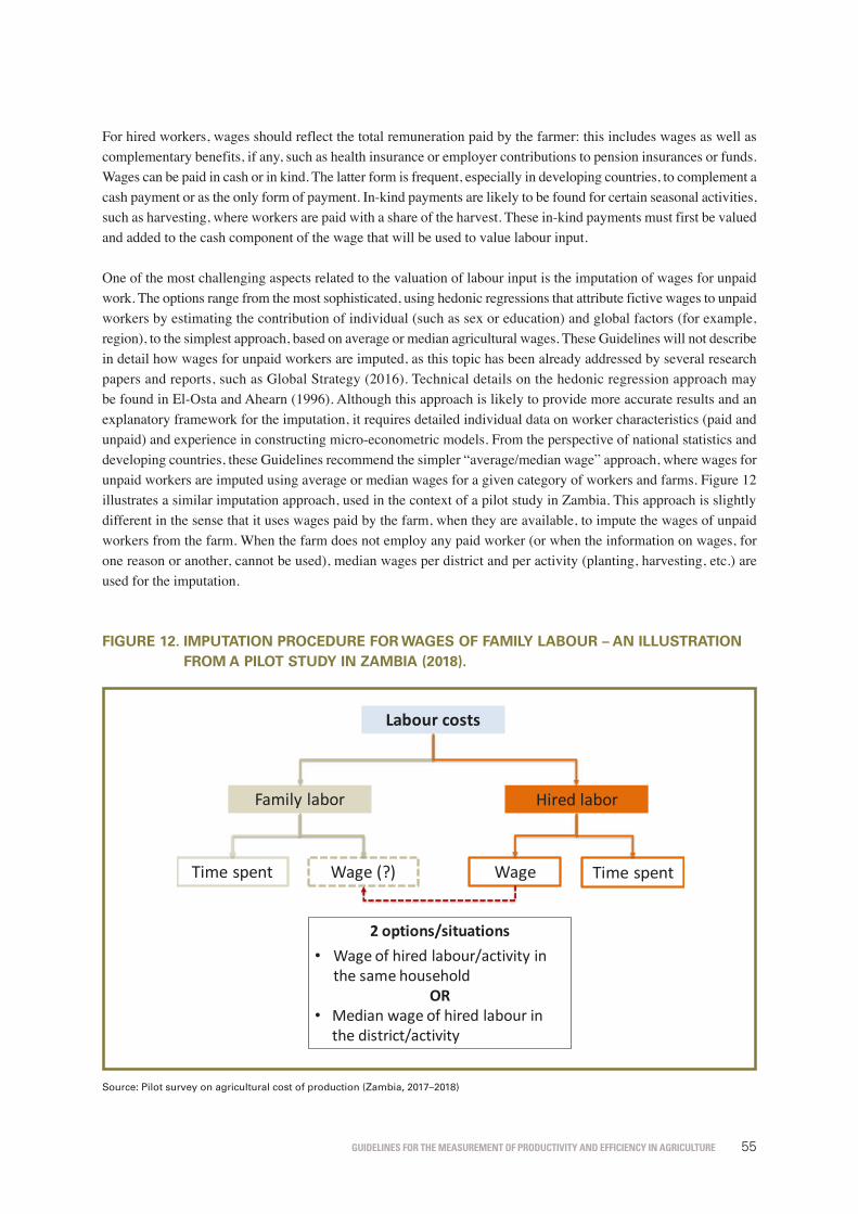
Guidelines for the measurement of productivity and efficiency in aGriculture 55
For hired workers, wages should reflect the total remuneration paid by the farmer: this includes wages as well as complementary benefits, if any, such as health insurance or employer contributions to pension insurances or funds. Wages can be paid in cash or in kind. The latter form is frequent, especially in developing countries, to complement a cash payment or as the only form of payment. In-kind payments are likely to be found for certain seasonal activities, such as harvesting, where workers are paid with a share of the harvest. These in-kind payments must first be valued and added to the cash component of the wage that will be used to value labour input.
One of the most challenging aspects related to the valuation of labour input is the imputation of wages for unpaid work. The options range from the most sophisticated, using hedonic regressions that attribute fictive wages to unpaid workers by estimating the contribution of individual (such as sex or education) and global factors (for example, region), to the simplest approach, based on average or median agricultural wages. These Guidelines will not describe in detail how wages for unpaid workers are imputed, as this topic has been already addressed by several research papers and reports, such as Global Strategy (2016). Technical details on the hedonic regression approach may be found in El-Osta and Ahearn (1996). Although this approach is likely to provide more accurate results and an explanatory framework for the imputation, it requires detailed individual data on worker characteristics (paid and unpaid) and experience in constructing micro-econometric models. From the perspective of national statistics and developing countries, these Guidelines recommend the simpler “average/median wage” approach, where wages for unpaid workers are imputed using average or median wages for a given category of workers and farms. Figure 12 illustrates a similar imputation approach, used in the context of a pilot study in Zambia. This approach is slightly different in the sense that it uses wages paid by the farm, when they are available, to impute the wages of unpaid workers from the farm. When the farm does not employ any paid worker (or when the information on wages, for one reason or another, cannot be used), median wages per district and per activity (planting, harvesting, etc.) are used for the imputation.
FIgure 12. ImputAtIon proCedure For wAges oF FAmIly lABour – An IllustrAtIon From A pIlot study In zAmBIA (2018).
Source: Pilot survey on agricultural cost of production (Zambia, 2017–2018)
59
Source: Pilot survey on agricultural cost of production (Zambia, 2017–2018)
4.4.2. Land
Land is a special type of asset: it cannot be moved (immobile) nor reproduced (that is, it cannot be produced artificially) and its main features (exposition, topology, soil composition, fertility, acidity, etc.) cannot be changed, or only marginally and at a very slow pace. Land has also an almost indefinite service life, contrary to other fixed or capital assets. Land is of course an essential asset for cropping activities and for livestock, as land is also used for grazing, pasture and for the cultivation of fodder crops.
Accounting for land in productivity measurement is essential, given the role it plays in the production processes of both crops and livestock. As for the other factors of production, the construction of productivity indicators requires data on “quantities”, which in the case of land refers to the concept of area, and prices or values. Data on land values are required to determine the input shares used to weight the changes in land area (or, if applicable, the changes in the area of the different types of land), as per the formula presented in box 2. This section describes the data needed on land input and prices and how it can be collected. Land input Land input is examined for both crops and livestock.
For crops
Land input refers to a measure of area of agricultural land. This measure of area can be used to construct land productivity indicators, or crop yields, and to account for land input in productivity measurement. The first choice that the data compiler must make refers to the concept of area. In agriculture, two types of area are often distinguished: cultivated area and harvested area. In this document, we refer to cultivated area for temporary crops as the sum of the area sown (or planted) as well as the land that is temporarily fallow. For permanent crops, cultivated area is simply the area planted with permanent crops. Harvested area can be equal to or less than cultivated area.
These Guidelines recommend using cultivated area to measure land input. The rationale for this recommendation is that many of the intermediate inputs such as agrochemicals, or factors of production such as labour or machinery, are used on the sown area (land preparation, seeding, fertilizer application, weeding, pesticide application, etc.). In addition, using harvested area instead of planted area risks leading to overestimations of yields and returns to land, as harvested
Labourcosts
Familylabor Hiredlabor
Timespent Wage(?) Wage Timespent
2options/situations• Wageofhiredlabour/activityin
thesamehouseholdOR
• Medianwageofhiredlabourinthedistrict/activity

Guidelines for the measurement of productivity and efficiency in aGriculture56
4.4.2. landLand is a special type of asset: it cannot be moved (immobile) nor reproduced (that is, it cannot be produced artificially) and its main features (exposition, topology, soil composition, fertility, acidity, etc.) cannot be changed, or only marginally and at a very slow pace. Land has also an almost indefinite service life, contrary to other fixed or capital assets. Land is of course an essential asset for cropping activities and for livestock, as land is also used for grazing, pasture and for the cultivation of fodder crops.
Accounting for land in productivity measurement is essential, given the role it plays in the production processes of both crops and livestock. As for the other factors of production, the construction of productivity indicators requires data on “quantities”, which in the case of land refers to the concept of area, and prices or values. Data on land values are required to determine the input shares used to weight the changes in land area (or, if applicable, the changes in the area of the different types of land), as per the formula presented in box 2. This section describes the data needed on land input and prices and how it can be collected.
Land inputLand input is examined for both crops and livestock.
For cropsLand input refers to a measure of area of agricultural land. This measure of area can be used to construct land productivity indicators, or crop yields, and to account for land input in productivity measurement. The first choice that the data compiler must make refers to the concept of area. In agriculture, two types of area are often distinguished: cultivated area and harvested area. In this document, we refer to cultivated area for temporary crops as the sum of the area sown (or planted) as well as the land that is temporarily fallow. For permanent crops, cultivated area is simply the area planted with permanent crops. Harvested area can be equal to or less than cultivated area.
These Guidelines recommend using cultivated area to measure land input. The rationale for this recommendation is that many of the intermediate inputs such as agrochemicals, or factors of production such as labour or machinery, are used on the sown area (land preparation, seeding, fertilizer application, weeding, pesticide application, etc.). In addition, using harvested area instead of planted area risks leading to overestimations of yields and returns to land, as harvested area often includes the most productive segments of the parcel. These Guidelines also recommend including land temporarily fallow (for less than five years) in the cultivated area: parcels are often left uncultivated for some time, to allow for the regeneration of soils and maintain their fertility. This strategy is therefore part of production technology and must be accounted for in the measurement of land and agricultural productivity.
Land input must be expressed in a meaningful unit. Unlike labour input, which can be reported in several units (number of employed persons, number of days, months, etc.), land area is typically measured in standard units such as acres or hectares. In certain countries, specific units can be used, such as feddan in Egypt or bigha in India. For data collection, it is recommended to use the unit with which the farmer feels more comfortable. When compiling the data, country-specific units can be converted to standard units such as acres or hectares to facilitate comparisons and analysis. From the perspective of productivity calculation, the choice of unit is not paramount, as long as the same unit is used consistently throughout the different data collection systems and data sets. It is important to ensure consistency in the data reported for land input with other variables with which it could be combined in the process of constructing productivity statistics. In particular, consistency between the area unit and the unit used for land rents is necessary to attach a value to land input.
For livestockLand is also a factor of production for livestock activities. Land can be used by animals to graze (pasture land) or cultivated by the farmer to grow crops that will be used to feed livestock (fodder crops).

Guidelines for the measurement of productivity and efficiency in aGriculture 57
In the raising of ruminants and, to a smaller extent, poultry, production systems are largely determined by the extent to which land is used for grazing (for ruminants) or scavenging (for poultry): the amount of land used to raise cattle, sheep or other ruminants may be negligible in the case of systems mostly based on stall-feeding, where the feed comes from concentrates or fodder crops produced by the farm or purchased from the market. On the contrary, in extensive grazing-based systems or for free-range chicken production, the land input is necessarily higher. These differences in production systems mechanically bear an impact on any land productivity measure for the livestock sector, as they directly affect the denominator of the indicator. These differences are partly levelled when all inputs and factors of production are considered. Indeed, in production systems based on grazing or scavenging, which typically exhibit low land productivity, the need for additional inputs such as fodder crops or feed concentrates is lower than when animals are mostly or exclusively raised in a confined environment. Given the influence of the production system (outdoor, indoor, mixed) on land productivity for livestock, and the balancing effects at play (low land input and high feed expenses, and vice versa), these Guidelines do not recommend compiling land productivity (a partial measure of productivity) for the livestock sector. However, pasture land used for grazing or land used to let chickens and other animals scavenge should be measured and included in TFP metrics for the livestock sector.
It is also important to indicate that, in line with the SNA, the cultivation of fodder crops should be categorized under crop production even though the destination of this produce is the livestock sector. In the measurement of productivity for the livestock sector, the use of fodder crops is accounted for, as all the other intermediate inputs, in the denominator of the indicator (if the gross output approach is used) or in the numerator (if the value-added concept is used). The mode of acquisition or supply of this input should not, in principle, affect the results: whether fodder crops are purchased from the market or produced by the farm itself, the amount used should always be recorded as an input into the livestock activity. In the case of farms producing their own feed, the different enterprises (for example, crop and livestock enterprises) must be separated to derive sector-specific data on output, production costs and productivity.
Land pricesDetermining the area used for crops or as pastureland is relatively straightforward. This information is collected by most, if not all, agricultural surveys, at least for cropping activities. With this data, basic land productivity measures such as crop yield (for example, output per hectare) can be calculated. To compute the TFP or other aggregate productivity measures that require aggregating and weighting different inputs, a value must be attributed to land.
This is a more complex operation, for several reasons. First, land ownership rights are often not well defined in many developing countries, where formal land titles or rental contracts are not common. Second, special forms of land ownership, such as communal, traditional or religious land, which are widespread in developing regions, are not well adapted to market valuation. Third, even when land ownership is well defined, markets for land (for rent or purchase) are often thin or inexistent, impeding the determination of representative rates. Fourth, land values vary greatly according to the characteristics of the land, such as the existence of land markets in the countries, the edaphic characteristics of the soil or the location of the land (its proximity to urban centres, transport infrastructure, etc.). For these reasons, the inclusion of land as a factor of production in MFP measurement poses several challenges, especially in countries dominated by small-scale and traditional agriculture.
To ensure consistency with the other inputs, the value of agricultural land should refer to its usage price for one agricultural season, calendar year or any other reference period chosen for the measurement of productivity. The rental value of the land is an adapted metric, as it reflects land quality characteristics and other market factors that influence land prices.

Guidelines for the measurement of productivity and efficiency in aGriculture58
Taking a bottom-up perspective to productivity measurement, starting with the basic data on agricultural area at farm level, valuing land can be done in different ways depending on the ownership status: for farmers renting land for agricultural purposes, the rental rates should be reported and used to value land. In the frequent cases where part or the totality of the rent is paid in kind, for example in the form of a share of the harvest, a cash equivalent must be calculated.
For landowners, a rental value should be imputed. Land rents provide a good approximation of the opportunity cost associated with land ownership. Indeed, the main alternative offered to owners of agricultural land is often to rent their land to other farmers, to cultivate it or use it as pastureland. Using rents to impute a value to owned land is therefore theoretically grounded and an acceptable estimation strategy. As for the estimation of fictive wages for unpaid labour, a rent can be imputed to owned land using simple techniques, such as the median or average rental rate per hectare or acre for similar land in the same region, or more sophisticated approaches based on econometric models. From the point of view of national statistics in developing countries, the use of practical and cost-efficient statistical techniques should be privileged over sophisticated approaches, which are better suited to academic research. In this perspective, these Guidelines recommend using simpler approaches based on average or median rental rates.
4.4.3. Fixed assetsFixed assets used in the production of crops and livestock are defined in section 2.10. This subsection presents the approaches recommended by these Guidelines to capture the contribution of farm capital to productivity growth, consistently with other agricultural inputs and factors of production.
As a preliminary remark, it is worth redefining the scope of the assets that ought to be considered in productivity measurement. First, the inclusion of capital in productivity measurement is usually restricted to farm buildings, machinery and equipment; while hired and owner-supplied labour can also be a form of capital (human), it is considered a separate factor of production and measured as labour input (OECD, 2001). These Guidelines adopt the same approach. Second, tree stock and orchards, as well as livestock, can also be a capital stock when they result from an investment (purchase of animals or the establishment of a new plantation, for example) that leads to a regular flow of revenue or service (revenue from the selling of fruits or milk, or service provided by animal traction, for example). However, given the specificity of these assets, the fact that the measurement is particularly complex (especially in developing countries) and there are relatively few references on the subject, this subsection focuses on traditional assets such as machinery, equipment and buildings. Ball and Harper (1990) contains a specific discussion on livestock as capital assets.
The contribution of fixed assets to productivity is captured by the flow of services generated by the stock of capital owned by the farmer. The approximation of this service flow is done in two steps: (i) estimating the stock of capital used by the farmer; and (ii) attaching a value or cost to this stock.
Capital stockThe capital stock consists of all fixed assets – such as machinery, equipment, buildings and other structures used by the farm – that provide inputs in the form of capital services into processes of production. The stock of capital accumulates as new investments are made (purchase of capital) and, therefore, may be seen as the cumulative value of all past capital investments made in the industry.
Guidelines for the measurement of productivity and efficiency in aGriculture 59
Capital formation processTwo methods are generally used to measure capital stock: the Perpetual Inventory Method (PIM) and the Current Inventory Method (CIM). The PIM measures the stock of capital as the sum of the current and depreciated past investments, while the CIM is based on the count and valuation of the set of capital goods owned and used by the farm. The choice of method essentially depends on the purpose of productivity measurement and the data available. For example, if the objective is to construct a macroeconometric model, PIM is probably the best approach to measure capital stock, as it ensures consistency with the overall macroeconomic accounting framework (between investment flows and capital formation, between interest rates, investments and capital formation, etc.). In principle, PIM can also be applied to farm-level series of investments in capital assets. When such detail is available, however, CIM is often preferred as it provides a more objective measure of capital stock at farm level. These Guidelines recommend using CIM when working directly from farm-level data, provided that proper information on assets and asset prices is available. Conversely, PIM should be used when working with aggregate series on investment. These two approaches are described below.
In PIM, the estimate for the current year’s new investment is added to the previous year’s stock. The productive capital from the previous year must be depreciated by one year as it is moved forward. In mathematical terms, this process is formalized as follows:
62
in productivity measurement. First, the inclusion of capital in productivity measurement is usually restricted to farm buildings, machinery and equipment; while hired and owner-supplied labour can also be a form of capital (human), it is considered a separate factor of production and measured as labour input (OECD, 2001). These Guidelines adopt the same approach. Second, tree stock and orchards, as well as livestock, can also be a capital stock when they result from an investment (purchase of animals or the establishment of a new plantation, for example) that leads to a regular flow of revenue or service (revenue from the selling of fruits or milk, or service provided by animal traction, for example). However, given the specificity of these assets, the fact that the measurement is particularly complex (especially in developing countries) and there are relatively few references on the subject, this subsection focuses on traditional assets such as machinery, equipment and buildings. Ball and Harper (1990) contains a specific discussion on livestock as capital assets.
The contribution of fixed assets to productivity is captured by the flow of services generated by the stock of capital owned by the farmer. The approximation of this service flow is done in two steps: (i) estimating the stock of capital used by the farmer; and (ii) attaching a value or cost to this stock.
Capital stock The capital stock consists of all fixed assets – such as machinery, equipment, buildings and other structures used by the farm – that provide inputs in the form of capital services into processes of production. The stock of capital accumulates as new investments are made (purchase of capital) and, therefore, may be seen as the cumulative value of all past capital investments made in the industry.
Capital formation process
Two methods are generally used to measure capital stock: the Perpetual Inventory Method (PIM) and the Current Inventory Method (CIM). The PIM measures the stock of capital as the sum of the current and depreciated past investments, while the CIM is based on the count and valuation of the set of capital goods owned and used by the farm. The choice of method essentially depends on the purpose of productivity measurement and the data available. For example, if the objective is to construct a macroeconometric model, PIM is probably the best approach to measure capital stock, as it ensures consistency with the overall macroeconomic accounting framework (between investment flows and capital formation, between interest rates, investments and capital formation, etc.). In principle, PIM can also be applied to farm-level series of investments in capital assets. When such detail is available, however, CIM is often preferred as it provides a more objective measure of capital stock at farm level. These Guidelines recommend using CIM when working directly from farm-level data, provided that proper information on assets and asset prices is available. Conversely, PIM should be used when working with aggregate series on investment. These two approaches are described below.
In PIM, the estimate for the current year’s new investment is added to the previous year’s stock. The productive capital from the previous year must be depreciated by one year as it is moved forward. In mathematical terms, this process is formalized as follows:
𝐾𝐾7) = 𝐼𝐼7) + 1 −𝜇𝜇7 𝐾𝐾7,)b< [4]
where 𝐾𝐾7) is the current year’s stock of asset 𝑖𝑖 (𝐾𝐾7,)b< the stock of the previous year), 𝐼𝐼7) the current year’s investment (i.e. asset purchases) in asset i, and 𝜇𝜇7 the depreciation rate associated with the asset.
The relevance of this calculation procedure depends on how well investments are captured and how realistic the assumed depreciation rates are. Capturing investments in agriculture is relatively
where Kit is the current year’s stock of asset i (Ki,t-1 the stock of the previous year), Iit the current year’s investment (i.e. asset purchases) in asset i, and μi the depreciation rate associated with the asset.
The relevance of this calculation procedure depends on how well investments are captured and how realistic the assumed depreciation rates are. Capturing investments in agriculture is relatively straightforward as it involves gathering data either from the farmers themselves or from input suppliers on the purchases (or sales, if the question is asked to suppliers) of machinery and equipment. This information can be obtained directly from farm or supplier surveys. Investments in new or improved infrastructure may also be collected from the farmers, through questions related to construction costs, or from service providers.
The determination of appropriate depreciation rates is a delicate matter, as the speed at which assets depreciate vary greatly depending on the type of asset. These Guidelines recommend differentiating the depreciation rates by asset classes, acknowledging that the first best approach, which consists in following the market prices of individual assets by millésime (by purchase year), would be prohibitively costly. Simple rules can help data compilers to choose an appropriate set of depreciation rates. For example, large assets typically have lower depreciation rates than smaller assets, as they are generally used for longer periods and therefore need to be replaced less frequently. Examples of asset classes may be “Small farm machinery and equipment used for crops”, “Large machinery and equipment used for crops”, “Irrigation equipment” and any other asset breakdown that is relevant from a service and asset size perspective. In addition to the choice of a set of annual depreciation rates, for a correct interpretation of the results, it is also necessary to understand how the depreciation of a given group of assets evolves through time. For instance, the capital accumulation process described by equation [4] assumes a geometric depreciation schedule, with compounded rates year after year applied to the initial investment. This means that while the annual depreciation rates remain the same (for example, 5 percent), each asset class is depreciated by decreasing absolute amounts each year.8 This is the approach adopted by Statistics Canada and the European EUKLEMS project, for example (Biatour et al., 2007).
8 For the first accounting period, the capital stock is equal to the initial investment:
each asset class is depreciated by decreasing absolute amounts each year.1 This is the approach adopted by Statistics Canada and the European EUKLEMS project, for example (Biatour et al., 2007).
When working with farm-level data for individual assets, it may be possible to directly measure the capital stock for a given farm and at one point in time: this is CIM. The data required to measure the value of the inventory is an estimate of the market value of the assets at a given point in time (time of the survey or any other reference period). This information can be asked from the farmer directly, by type of asset to facilitate recall and reporting, similarly to the Zambia Post-Harvest and Livestock Survey Questionnaire (figure 13). In this example, the farmer is asked about the assets owned (tractors, rippers, etc.) and an own estimate of the price that they might receive on the market. The advantages of this approach are that it comprehensively covers the farm assets, and that the estimate of capital stock is based on actual market prices. Market prices, by construction, reflect depreciation resulting from aging as well as from any obsolescence factor, for example the introduction of new, more efficient and perhaps cheaper assets. This estimate is therefore a good reflection of the stock of physical assets, the assets’ condition and age, as well as of the market dynamics at play.
1 For the first accounting period, the capital stock is equal to the initial investment: 𝐾𝐾" = 𝐼𝐼"; in period 2: 𝐾𝐾% = 𝐼𝐼% + 1 − 𝜇𝜇 𝐾𝐾" = 𝐼𝐼% + 1 − 𝜇𝜇 𝐼𝐼"; in period 3: 𝐾𝐾+ = 𝐼𝐼+ + 1 − 𝜇𝜇 𝐾𝐾% = 𝐼𝐼+ + 1 − 𝜇𝜇 %𝐼𝐼" + 1 − 𝜇𝜇 𝐼𝐼%; by way of recurrence, for a given period 𝑡𝑡: 𝐾𝐾- = 1 − 𝜇𝜇 -./𝐼𝐼/-
/0" .

Guidelines for the measurement of productivity and efficiency in aGriculture60
When working with farm-level data for individual assets, it may be possible to directly measure the capital stock for a given farm and at one point in time: this is CIM. The data required to measure the value of the inventory is an estimate of the market value of the assets at a given point in time (time of the survey or any other reference period). This information can be asked from the farmer directly, by type of asset to facilitate recall and reporting, similarly to the Zambia Post-Harvest and Livestock Survey Questionnaire (figure 13). In this example, the farmer is asked about the assets owned (tractors, rippers, etc.) and an own estimate of the price that they might receive on the market. The advantages of this approach are that it comprehensively covers the farm assets, and that the estimate of capital stock is based on actual market prices. Market prices, by construction, reflect depreciation resulting from aging as well as from any obsolescence factor, for example the introduction of new, more efficient and perhaps cheaper assets. This estimate is therefore a good reflection of the stock of physical assets, the assets’ condition and age, as well as of the market dynamics at play.
FIgure 13. extrACt From the seCtIon on FArm Assets oF the zAmBIA post-hArvest QuestIonnAIre.
Source: Zambia Post-Harvest Survey (pilot survey, 2017–2018)
Capital stock in constant pricesThe measures of capital stock presented above are necessarily expressed in monetary units. Given the diversity of the services provided by each asset, the use of alternative common units (horsepower, volumetric capacity of storage facility or of crop processing equipment such as shellers, driers, etc.) is indeed difficult. To assess the contribution of fixed assets to productivity, distortions created by asset price changes must be removed in order to approximate the changes in the physical stock of assets. To this end, capital stock should be measured at prices referring to a fixed period (constant prices). As the basic data on investments (for PIM) or on market prices (for CIM) are most likely expressed in prices of the current period, the time series must be deflated by a proper price index, to reconstruct a volume measure of capital stock. As for the other factors of production and inputs, it is advised to ensure the best possible match between the scope of the deflator and the scope of the phenomenon of interest: the price index for capital goods would be the ideal deflator (even better, if it concerns the agricultural sector specifically); however, it is likely to be unavailable. Alternatives can be a price index for industrial goods or, as a last resort, the GDP deflator.
Capital serviceThe contribution of the farm assets to production and productivity is captured through the amount of services that they provide. The services rendered by fixed assets can be observed and measured in physical terms, for example the number of hectares covered by a combine harvester during a year, the tons of crops that can be processed by a mechanical thresher, the litres of milk that can be obtained from the stock of milking machines, etc. However, in most cases, the flows of capital services are not directly observable and, even if they were, they would be expressed in many different units, impeding aggregation across asset groups.

Guidelines for the measurement of productivity and efficiency in aGriculture 61
The most common approach is to approximate capital services as a proportion of the stock of capital, this proportion being equal to the rental value that can be extracted from the asset stock during a given reference period. This is a rather intuitive concept that can be illustrated by the following example. Consider a farmer who declares that the combine harvester and the planter owned by the farm would be worth 1 000 on the market, at current prices. These two assets therefore represent a stock of capital of 1 000. The same farmer then estimates that he could receive 100 if he were to rent these two assets to another farmer during the agricultural season. The services generated by these two assets are then assumed to be 100, or 10 percent of the stock of capital. This approach can be used to estimate capital services from the basic data collection level. While these rental rates can in principle be obtained for each farmer through direct enquiry, it is advised that standard or average rates by type of asset be determined and used consistently over the sample of farms, to avoid possible noise due to reporting issues and to compute consistent measures of capital services.
When working from aggregated capital stock series, constructed using PIM, similar rates can be used to construct a measure of capital services. In this setting, it is more intuitive to think of the proportion of capital stock as a measure of the intensity at which the capital is used. Taking the same example of the previous paragraph, if a rental rate of 10 percent is used, it also means that 10 percent of the capital stock is used during the reference period: in other words, the intensity ratio is 10 percent. Information on intensity ratios can be obtained or estimated by asset type, as certain assets are used more intensively than others.
Once capital services at current prices have been determined, they must be deflated to construct a measure of volume of services, which will then be used in the productivity measurement calculation. The most appropriate deflator would be a price index for providers of agricultural services.9 An alternative could be to use a producer price index for agricultural input providers (including agricultural inputs, machinery, equipment and services). As a last resort, the deflator of the agricultural GDP or of total GDP can be used.
4.5. workIng wIth AggregAted tIme serIes
This chapter has considered that the building blocks for productivity measurement – quantity or volume measures of input and value-weights – could be constructed bottom-up, using mostly farm-level information on output by commodities (physical quantities and selling prices) and on individual intermediate inputs and factors of production (quantities or amounts and purchase prices). This may be possible in certain circumstances; however, in most cases, statisticians or analysts involved in productivity measurement must work with aggregated time series and spend most of their time identifying the best ways to reconstruct values or volumes using the best price-volume split approach (that is, using the most suitable price information). For example, the construction of a volume measure of inputs, which is required for the measurement of productivity, may either result from the valuation of physical quantities from the basic item level (the ideal case) or from input values deflated by an aggregate price index. This section provides basic guidance to users dealing with aggregated time-series and the unavailability of detailed information on input quantities and prices. On the output side, the availability of information is generally higher, and adequate information can normally be found on the physical quantities and selling prices for most important agricultural commodities.
9 In national accounts, this sector is a subset of the “business services” sector.
Guidelines for the measurement of productivity and efficiency in aGriculture62
The cases of labour and land are discussed, which present specificities regarding the availability of information and the process to construct quantity, volume and value time series. Insights for fixed assets are provided in section 4.4.3. For the other inputs or factors of production, the process is similar, the specificities lying mostly in the choice of an adapted deflator.
LabourIn the subsection on labour, the recommendations referring to the measurement of labour input and its valuation using appropriate wages assumed that data would be available at the most granular level, which can be the field, farm or agricultural household. Data with this level of granularity is typically obtained from agricultural or household surveys.
However, officers in charge of the compilation of productivity statistics often work from pre-aggregated and compiled time series on labour, and not directly from the farm-level data. The assumption is that the preliminary work of measuring labour input and wages, and related calculations and imputations, have already been done by the statisticians in charge of the farm surveys. As a result, the officers in charge of compiling productivity statistics may have to work directly from aggregated time series on labour expenses in the agricultural sector, probably combining different types of labour and wages. Regarding labour, aggregate or average data are typically available on labour wages or expenses, although not on labour input (in months, days or full-time equivalents, for instance). In this case, the construction of a volume measure of labour requires deflating the time series of expenses with an appropriate price index. The price index should be as close as possible to the phenomenon that is being measured. For example, an index of wages in the agricultural sector would be an ideal candidate for a deflator. However, in the frequent cases where wage indexes for the agricultural sector are not available, the data compiler is obliged to revert to second- or third-best options, such as wages referring to the entire economy or to sectors for which this information is readily available (for example, wage indexes for the industrial or service sectors). This of course has implications for the quality and interpretability of the results.
LandData compilers are likely to face aggregated data on agricultural area, with little detail on the characteristics of the land except its breakdown by crop or pastureland. Aggregate information on land prices or rents is unlikely to be available, reflecting the different types and qualities of agricultural land, for example in the form of a price index. In this situation, additional information on prices for agricultural land must be gathered. Ideally, the level of detail in the rents must match the breakdown provided for the area data: if the latter is available by crop, it should be combined with the rents per hectare of cultivated crop. The higher the disaggregation of area and price data, the better will the land value indicator reflect the different quality characteristics of the land. On the contrary, if weights are based on average rents without distinction by crop or other factors that may affect land prices, the weighting scheme will be distorted and the final measure of productivity flawed.

Guidelines for the measurement of productivity and efficiency in aGriculture 63
4.6. dAtA sourCes And ConsIstenCy
The measurement of agricultural productivity relies on multiple variables: agricultural outputs, intermediate inputs, factors of production and their respective prices, wages or rental values. The basic information on these different components is unlikely to be found in a single data source, such as an agricultural production survey, but rather from a variety of sources of information and data sets. Some of the main sources of data are identified in section 3.2. The objective of this section is to: (i) discuss the extent to which this diversity in data sources affects the quality of the final productivity indicators; and (ii) provide guidance to data compilers on how to ensure the maximum level of consistency in the calculation of agricultural productivity.
Multiple sources of information, with varying characteristicsBeyond the calculation process and algorithms, the most challenging aspect of productivity measurement is, perhaps, the need to deal with a variety of data sources. Working with different sources of information does not necessarily mean that the data will be of uneven quality, if the appropriate statistical coordination and quality frameworks are in place and function well. In practice, however, when data are collected separately, they tend to rely on a set of characteristics or properties that are relevant to the specific phenomenon that is being measured. These characteristics and properties may refer, for example, to the basic definitions of statistical units, the reference periods, the base periods, the different types of data collection mechanisms (sample surveys, administrative records, experts opinion, etc.) and their respective properties (for example, whether statistically representative or not), different levels of aggregation (micro- or farm-level, meso-level, macro-level) and different rules in terms of calculating intermediate and final indicators.
A typical example in the agricultural context is the use of data from both household and agricultural surveys: the main statistical unit in household surveys is the household, whereas agricultural surveys may rely on different units: the agricultural household (typically broader than the household, strictly speaking), the farm, the enterprise (specific farm activity), the field, etc. The reconciliation between the data collected for different units is not necessarily straightforward and may require certain assumptions. For example, in the context of surveys in developing countries focusing on smallholders, the assumption is that a one-to-one relationship exists between the household and the agricultural holding. Other examples are input prices, which may be available only in the form of averages at high geographical levels or for aggregated product categories, and thus not necessarily reflecting the purchase prices effectively paid by farmers.
The construction of productivity indicators also requires working with statistical information available at different levels of aggregations or granularity, from the lowest micro unit to the highest macroeconomic level. These Guidelines describe the productivity compilation process from different aggregation perspectives: bottom-up, working from microdata up to the sector level, and directly from macroeconomic time series, the approach traditionally used in the field of national statistics. While the philosophy of the approach remains the same (constructing quantity or volume measures of outputs and inputs and weighting them to obtain a global measure of productivity growth), the process is different: the micro approach requires the computation of volumes and values at farm, activity or crop level using detailed quantity and price information (likely to come from farm surveys), while the macro approach is based on the processing of macroeconomic time series to determine volume and value measures (volume-price split), typically through the identification of the most appropriate deflators.
Ensuring minimal consistency in the basic dataBefore embarking upon the calculation of productivity indicators, a considerable amount of preliminary data processing and manipulation is necessary to ensure the maximum level of consistency across these different sources of data and to minimize noise in the final productivity indicators. This preliminary phase includes activities such as rebasing (to ensure that common base periods are used), retropolations or extrapolations to obtain time series of similar lengths, estimations of missing information as well as aggregations or, on the contrary, breaking down statistical information. The following paragraphs discuss some of the most important dimensions relating to data quality, for which data compilers need to seek the maximum level of consistency.

Guidelines for the measurement of productivity and efficiency in aGriculture64
Reference periodsData on agricultural outputs and inputs should refer to the same period: calendar year, agricultural year, summer or winter season, etc. To compute meaningful productivity indicators, the period of reference of the statistical information for the numerator (output) should correspond to the period of reference for the denominator (input). This may seem an obvious statement; however, because of the unavailability of information, this condition is often not met, at least in part. If “hard” data is not available for the same years or reference periods, appropriate estimation methods (retropolations, extrapolations, estimations), should be devised to fill in the gaps. For example, variables such as production or input use often refer to the agricultural season (and even to subseasons, such as the winter or summer season), while information on prices, wages or assets is more often found for the calendar year. In these situations, the necessary adjustments should be made to ensure proper matching between the reference periods.
Base periodsCalculating the TFP requires the aggregation of output volumes – using their respective value shares as weights – and the aggregation of inputs using expense shares. It is important that the weights for the outputs and inputs refer to the same period (the base period) to ensure consistency in the numerator and denominator and to facilitate the interpretation of the results. This means that information on prices, which is necessary to construct values, should be available for the same years. Where information for certain years is not available or scarce, these Guidelines recommend choosing a different base period, with better data availability. It is not recommended to attempt estimating missing prices for missing years, as they are typically difficult to impute given their high variability.
Index construction methodsConsistency in the data also extends to the way indexes of outputs and inputs are formed or, in other words, to the weighting scheme used. For instance, if a Laspeyres approach is used (therefore, the beginning of period value shares) to weight output changes, the same approach should be used to establish expense shares for inputs.
Sectoral scopeEnsuring consistency in the scope of the different variables is also key to ensuring high-quality and usable results, with minimal bias. Given the diversity of the data items that enter the process of calculating productivity, ensuring consistency in the sectoral boundaries may not be as straightforward. For example, some of the data may be obtained from agricultural surveys, which may focus mostly on the small-scale or subsistence sector, and thus not be representative of the agricultural sector as a whole. Indeed, in many developing countries, different data collection systems cover the subsistence and the commercial or large-scale sector, given the vast differences between these two sectors in terms of farming practices and yields. Data on farm assets or land rents, for example, may only be available for the commercial sector. To the greatest extent possible, data compilers should avoid combining data that refer to different scopes, for example data on output from the subsistence sector and data on fixed assets or land rents from the large-scale sector. If “hard” data for one or the other sector are unavailable, estimating the missing information using auxiliary information should be attempted, to enforce consistency. If this is not possible with an acceptable level of accuracy, data compilers should, as a last resort, explain the possible differences in scope in the metadata reports, and assess their possible impact on the final indicators, in both quantitative and qualitative terms.
Ensuring consistency in the overall data collection and compilation process requires a significant amount of data processing, as well as a good knowledge of the data construction mechanisms and of the accounting rules governing the compilation of economic indicators at different aggregation levels. Therefore, it is essential to foster interaction with teams working on national accounts, as national accountants are used to working with a variety of data sources and performing reconciliation exercises that aim at enforcing compliance with the accounting principles prescribed at national and international level by the SNA.
Guidelines for the measurement of productivity and efficiency in aGriculture 65
4.7. summAry oF reCommendAtIons
Box 8. summAry oF reCommendAtIons.
Agricultural output• All agricultural output of the farm should be accounted for, irrespective of the relative importance of each
product and of their destination (home consumption, use as intermediate inputs, selling, storage).• To the extent possible, the output should be measured net of harvesting losses and net of other on-farm losses
(this also applies to livestock products, such as milk).• Transformed products (butter, maize flour, etc.) should not be part of agricultural output.
Intermediate inputs• All intermediate inputs used to cultivate crops (such as seeds and fertilizers) and to raise livestock (feed, etc.)
must be covered, irrespective of their mode of acquisition: purchased (from the market, from the government, etc.) or self-supplied (livestock manure used as fertilizers, etc.).
• Intermediate inputs should be valued at the price effectively paid by the farmer (purchase price): if the inputs are subsidized, the subsidized price must be recorded. It is good practice to also collect the amounts of subsidies spent on intermediate inputs separately.
• The price of self-supplied inputs (organic manure, feed for livestock, etc.) should be imputed using average market prices for the respective inputs.
Labour• The amount of labour used for farming (labour input) should be measured with the most precise time unit
possible, such as number of hours or number of days, for both paid and unpaid workers.• Unpaid labour (such as household labour) should be valued at the median or average wages prevailing in
the region.• To account for quality differences in labour, quality attributes should be collected for the different farm
workers (education, experience in farming, etc.).
Land• For crops, land input should be measured in terms of area of cultivated land.• For livestock, the area used for grazing should be collected, in addition to information on the production
system (fully confined, partly confined, free-range, etc.)• A land productivity indicator for the livestock sector is not easily interpretable, given the separation of
production systems (for example, confined versus grazing). However, land input for livestock should be included in any TFP-like productivity measure covering this sector.
• Rents paid to cultivate land or use it for grazing should be used for valuation. For owned land, average or median rental rates by activity or crops can be used.
Fixed assets• The contribution of assets to the farm’s agricultural output is measured on the basis of the services provided
during the agricultural season by the stock of assets. • This stock is measured using CIM, if microdata is available, or PIM, if macroeconomic time series are used.• Capital services are determined as a proportion of the stock of assets, typically reflecting the rental value of
these assets during a full agricultural season.

Guidelines for the measurement of productivity and efficiency in aGriculture66

Guidelines for the measurement of productivity and efficiency in aGriculture 6767
ConclusionsThese Guidelines seek to walk readers through the various steps of the process of compilation of agricultural productivity. Chapter 2 defines productivity, presents the conceptual measurement framework and delimits the scope of this statistical activity. Chapter 3 details the different indicators and provides guidance on the choice of the metrics, in function of the objectives of the statistical program and the resources available. Finally, Chapter 4 presents the data requirements for outputs and inputs, highlighting best practices and second- or third-best approaches, as well as the implications for statistical quality and data collection requirements of each of them.
We believe that the value added by this document does not lie in the level of its theoretical developments or in the level of mathematical formalization, which has been kept at the minimum required for national statisticians, our main target audience, to fully understand the calculation procedures and to be in a position to replicate the different steps of the calculation, and to make informed choices regarding indicators and data at each stage. Readers are systematically referred to other reports, such as OECD (2001) or research publications, for details on the technical and mathematical grounding of the calculation procedures, for example on index number theory.
Readers interested in building productivity indicators for the agricultural sector are provided with: (i) the tools to understand the conceptual framework and set the scope of this statistical activity (chapter 2); (ii) guidance on which indicator to choose depending on the objective of the program, the information available and the financial and technical resources available (chapter 3); and (iii) guidance on the type of data to collect and how to collect it, as well as on the implications of choosing one option (for example, second-best) on data collection costs and complexity as well as on the quality of the final statistics. This report has also taken a double perspective regarding the construction and analysis of productivity: bottom-up, working from microdata, and directly from macroeconomic time series, when most of the publications destined to statistical organizations in this field focus on the latter.
This document intentionally leaves aside important components of productivity measurement, such as the contribution of environmental resources and assets to agricultural production and productivity, a topic that has drawn increasing attention from the research community and which still requires some development before it can be translated into operational calculation procedures that could be used by statistical or research officers of national organizations in developing countries.

Guidelines for the measurement of productivity and efficiency in aGriculture68
Agricultural & Applied Economics Association (AAEA). 2000. Commodity Costs and Returns Estimation Handbook. Task Force on Commodity Costs and Returns. AAEA Publication: Ames, IA, USA.
Ball, V.E. & Harper, M.J. 1990. Neoclassical Capital Measures Using Vintage Data: An Application to Breeding Livestock,U.S.BureauofLaborStatistics,OfficeofProductivityandTechnology:Washington,D.C.:Unpublished.
Ball, V.E., Nehring, R. & Wang, S.L. 2016. Productivity Growth in U.S. Agriculture: 1948-2013. International Productivity Monitor, 30: 64–76.
Biatour, B., Bryon, G. & Kegels, C. 2007. Capital Services and Total Factor Productivity Measurements: Impact of Various Methodologies for Belgium, Federaal Planbureau.
Cornwall, J. 1987. Total factor productivity, in The New Palgrave Dictionary of Economics, 4: 600-662, MacMillan Press, New York.
Diewert, W.E. 1980. Capital and the Theory of Productivity Measurement, The American Economic Review, 70(2): 260-67
Färe, R., Grosskopf, S., Lovell C.A.K., & Pasurka, C. 1989. Multilateral Productivity Comparisons when some Outputs are Undesirable: A Nonparametric Approach. Review of Economics and Statistics, 71(1): 90-98.
Food and Agriculture Organization of the United Nations (FAO). 1980. Farm and input prices: collection and compilation. FAO Economic and Social Development Paper no. 16. FAO Publication: Rome.
FAO. 1999.RegionalOfficeofAsiaandthePacific.Poverty alleviation and food security in Asia: role of livestock. Available at: http://www.fao.org/docrep/003/x6627e/x6627e00.htm. [Last accessed May 2018]
Farrell, M.J. 1957. Themeasurementofproductiveefficiency.Journal of the Royal Statistical Society, Series A, 120(3): 253–290.
Fraser, I. & Hone, P.2001.Farm-levelefficiencyandproductivitymeasurementusingpaneldata:woolproductionin south-west Victoria. The Australian Journal of Agricultural and Resource Economics, 45(2): 215–232.
Fuglie, K. 2015. Accounting for growth in global agriculture. Bio-based and Applied Economics. 4(3): 201–234.
Global Strategy to Improve Agricultural and Rural Statistics (GSARS). 2016. Handbook on Agricultural Cost of Production Statistics: Guidelines for Data Collection, Compilation and Dissemination. GSARS Handbook: Rome.
GSARS. 2017a. Productivity and Efficiency Measurement in Agriculture: Literature Review and Gaps Analysis. Technical Report no. 19. Global Strategy Technical Report: Rome.
GSARS. 2017b. Handbook on the Agricultural Integrated Survey. AGRIS Questionnaire – Labour Module. GSARS Handbook: Rome. Available at: gsars.org/wp-content/uploads/2018/02/AGRIS-LABOUR_QUEST-VERSION1-1.1-September-2017-final-EN-RA.xlsx.
References

Guidelines for the measurement of productivity and efficiency in aGriculture 69
GSARS. 2018. Guidelines on the Measurement of Harvest and Post-Harvest Losses. GSARS Guidelines: Rome.
Grosskopf, S. 2002. Some Remarks on Productivity and its Decomposition. Journal of Productivity Analysis, 20(3): 459–474.
Hayati, D. 2017. A Literature review on frameworks and methods for measuring and monitoring sustainable agriculture. GSARS Technical Report no. 22. GSARS Technical Report: Rome.
Kelly V., Hopkins J., Reardon T. & Crawford E. 1996. Improving the Measurement and Analysis of African Agricultural Productivity: Promoting Complementarities Between Micro and Macro Data. SD Publication Series. Technical Paper no 27. Department of Agricultural Economics, Michigan State University.
Lips, M. 2017. Disproportionate Allocation of Indirect Costs at Individual-Farm Level Using Maximum Entropy. Entropy, 19: 453.
Ludena, C.E. 2010. Agricultural Productivity Growth, Efficiency Change and Technical Progress in Latin America and the Caribbean. IDB Working Paper Series 186. Inter-American Development Bank, Washington, D.C.
OECD. 2001. Measuring Productivity – OECD Manual: Measurement of Aggregate and Industry-level Productivity Growth. OECD Publication: Paris.
OECD. 2002. Measuring the non-observed economy: a handbook. Available at: https://www.oecd.org/std/na/1963116.pdf.
OECD. 2015. Report on the OECD expert workshop on measuring environmentally adjusted agricultural total factor productivity and its determinants. OECD Publication: Paris
Nishimizu, M. & Page, J. 1982. Total Factor Productivity Growth, Technological Progress and Technical EfficiencyChange:DimensionsofProductivityChangeinYugoslavia,1965-78.TheEconomicJournal,92(368):920–936.
Prasada Rao, D.S. 1993. Intercountry comparisons of agricultural output and productivity. FAO Economic and Social Development Paper, no. 112. FAO Publication: Rome.
Rada, N. & Valdes, C. 2012. Policy, Technology and Efficiency in Brazilian Agriculture. ERR-137. Publication of the U.S. Department of Agriculture, Economic Research Service: Washington, D.C.
Sadoulet, E. & de Janvry, A. 1995. Quantitative Development Policy Analysis. The Johns Hopkins University Press: Baltimore, Maryland, USA and London.
Solow, R. 1957. Technical Change and the Aggregate Production Function. The Review of Economics and Statistics, 39(3): 312–320.

Guidelines for the measurement of productivity and efficiency in aGriculture70
layout: • Laura Monopoli
Cover photos:• © CIAT/Neil Palmer• © CIAT/Neil Palmer• © FAO/Giulio Napolitano

