C S I R O L A N D a nd WAT E R

Gully and Riverbank Erosion Mapping for the

Murray-Darling Basin

A.O. Hughes and I.P. Prosser

CSIRO Land and Water, Canberra

Technical Report 3/03, March 2003

Gully and Riverbank Erosion Mapping for the Murray-Darling Basin

A.O. Hughes and I.P. Prosser

CSIRO Land and Water, Canberra Technical Report 3/03, March 2003

Copyright ©2003 CSIRO Land and Water To the extent permitted by law, all rights are reserved and no part of this publication covered by copyright may be reproduced or copied in any form or by any means except with the written permission of CSIRO Land and Water.

Important Disclaimer To the extent permitted by law, CSIRO Land and Water (including its employees and consultants) excludes all liability to any person for any consequences, including but not limited to all losses, damages, costs, expenses and any other compensation, arising directly or indirectly from using this publication (in part or in whole) and any information or material contained in it. ISSN 1446-6163

I

Table of contents

Abstract ......................................................................................................................... 1

1 Introduction............................................................................................................ 1

1.1 Gully Erosion Assessment Method ................................................................... 2

1.2 Modelling techniques ....................................................................................... 2

1.3 Results of Gully Erosion Mapping ................................................................... 6

1.4 Time Sequence of Gully Erosion .................................................................... 10

2 Introduction to Riverbank Erosion ..................................................................... 12

2.1 MDB Assessment of Riverbank Erosion......................................................... 13

2.2 Bank Erosion Results ..................................................................................... 15

3 Conclusion............................................................................................................ 16

4 References ............................................................................................................ 19

1

Abstract This report presents gully and river bank erosion predictions for the Murray-Darling

Basin. The results in this report significantly improve upon those presented in the

NLWRA assessment. The predicted average gully density for the MDB is 0.08

km/km2. There are approximately 89,000 km of gully in total, which on average have

produced 13 million tonnes of sediment per year. In total, gullies in the MDB have

eroded 1.3 billion tonnes of sediment in historical times. Over the entire MDB the

new bank erosion methodology presented in this report predicts a mean annual rate of

sediment production from bank erosion of 8.6 Mt/y. This is 45% of the 19 Mt/y

predicted to be eroding from riverbanks in the original NLWRA assessment.

Comparing the new predictions of riverbank erosion with those of gully erosion

suggests that riverbanks supply 30% less sediment than gully erosion. In the

NLWRA assessment the predictions were more balanced with riverbank erosion

supplying 10% less. Overall the new assessment reduces the total load by almost

50%.

1 Introduction Gully and riverbank erosion are significant land degradation processes and sources of

sediment to Australian rivers. Increased sediment loads degrade downstream riverine

ecosystems by increasing turbidity and nutrient loads, and by smothering bed habitat,

which reduces the diversity of bedforms (Lemly, 1982; Galloway et al., 1996).

Erosion from stream and gully banks can generate up to 90 percent of the total

sediment yield from a catchment (Olley et al., 1993; Prosser and Winchester, 1996,

Wallbrink et al., 1998, Wasson, et al., 1998). Sediment that has been eroded from

gullies since European settlement is still present in many rivers and continues to

impact upon river ecosystems.

This study has produced predictions of gully extent across the Murray-Darling Basin

based upon extensive measurements from aerial photographs. Gully density

prediction was carried out via the generation of numeric rule-based predictive models.

These predictions of the location and extent of gully erosion should be useful in

regional planning of erosion control. Riverbank erosion was predicted from river

properties defined by the 9 second (approximately 250 m) resolution digital elevation

2

model for Australia, and other variables included in a simple conceptualisation of the

erosion process.

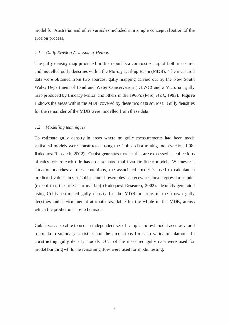
1.1 Gully Erosion Assessment Method

The gully density map produced in this report is a composite map of both measured

and modelled gully densities within the Murray-Darling Basin (MDB). The measured

data were obtained from two sources, gully mapping carried out by the New South

Wales Department of Land and Water Conservation (DLWC) and a Victorian gully

map produced by Lindsay Milton and others in the 1960’s (Ford, et al., 1993). Figure

1 shows the areas within the MDB covered by these two data sources. Gully densities

for the remainder of the MDB were modelled from these data.

1.2 Modelling techniques

To estimate gully density in areas where no gully measurements had been made

statistical models were constructed using the Cubist data mining tool (version 1.08;

Rulequest Research, 2002). Cubist generates models that are expressed as collections

of rules, where each rule has an associated multi-variate linear model. Whenever a

situation matches a rule's conditions, the associated model is used to calculate a

predicted value, thus a Cubist model resembles a piecewise linear regression model

(except that the rules can overlap) (Rulequest Research, 2002). Models generated

using Cubist estimated gully density for the MDB in terms of the known gully

densities and environmental attributes available for the whole of the MDB, across

which the predictions are to be made.

Cubist was also able to use an independent set of samples to test model accuracy, and

report both summary statistics and the predictions for each validation datum. In

constructing gully density models, 70% of the measured gully data were used for

model building while the remaining 30% were used for model testing.

3

Figure 1 Coverage and source of gully mapping data in the Murray-Darling Basin

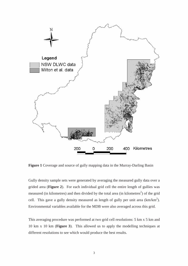
Gully density sample sets were generated by averaging the measured gully data over a

grided area (Figure 2). For each individual grid cell the entire length of gullies was

measured (in kilometres) and then divided by the total area (in kilometres2) of the grid

cell. This gave a gully density measured as length of gully per unit area (km/km2).

Environmental variables available for the MDB were also averaged across this grid.

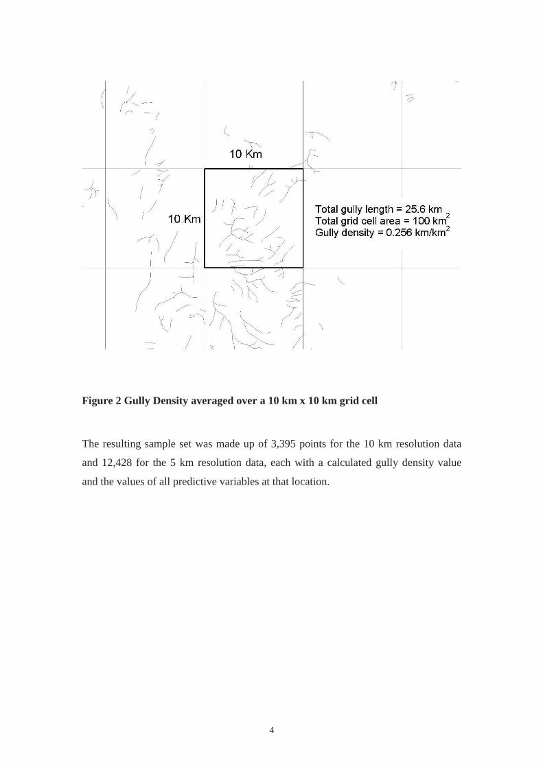
This averaging procedure was performed at two grid cell resolutions: 5 km x 5 km and

10 km x 10 km (Figure 3). This allowed us to apply the modelling techniques at

different resolutions to see which would produce the best results.

4

Figure 2 Gully Density averaged over a 10 km x 10 km grid cell

The resulting sample set was made up of 3,395 points for the 10 km resolution data

and 12,428 for the 5 km resolution data, each with a calculated gully density value

and the values of all predictive variables at that location.

5

Figure 3 Gully density for areas of measured data averaged over a) 5 km x 5km

and b) 10 km x 10 km

The predictive variables were selected to represent the factors that could potentially

control gully density. Fifteen variables were used for prediction:

• Two aggregated geology classifications derived from the 1:2,500,000 scale

geology map of Australia

• Three soil characteristics derived from the Atlas of Australian Soils – solum

thickness, A-horizon texture, B-horizon texture

• Six climate indices – Temperature seasonality, minimum temperature – coldest

period, temperature – annual change, mean annual precipitation, lowest period

moisture index, moisture index seasonality

• Contemporary landuse map produced by BRS

• Relief – slope and hill-slope length derived from the NLWRA topographic

analysis of the 9” DEM.

• Annual average contemporary ground cover as determined from the normalised

differential vegetation index (NDVI) derived from advanced very high resolution

radiometer (AVHRR) remote sensing.

6

To determine which of the above variables were actually important to predict gully

density, combinations of variables were tested. Examining all combinations of

variables was prohibitively time consuming, so a stepwise approach was used. For

the first step, each variable was used independently and the best variable identified

using statistical diagnostics from Cubist outputs (correlation and relative error). This

one variable was then used with each other variable, and the best second variable

identified. This process was repeated until all variables were included.

Final selection of the model was based on statistical diagnostics, and visual

comparisons of predicted and measured gully density maps.

1.3 Results of Gully Erosion Mapping

The best results, in terms of both correlation coefficients and spatially coherent

patterns were consistently produced by the 10 km x 10 km model runs. Table 1 shows

the best model results for the 5 km resolution and 10 km resolution model runs.

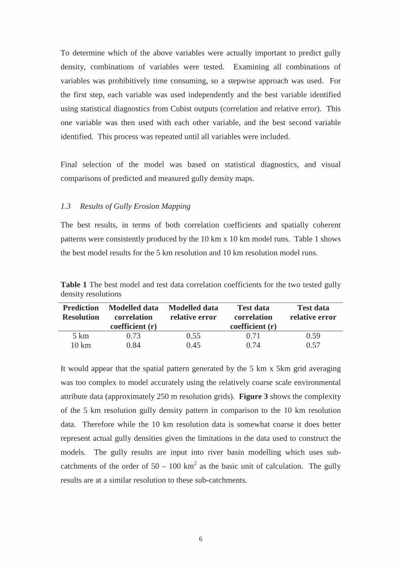
Table 1 The best model and test data correlation coefficients for the two tested gully density resolutions

Prediction Resolution

Modelled data correlation

coefficient (r)

Modelled data relative error

Test data correlation

coefficient (r)

Test data relative error

5 km 0.73 0.55 0.71 0.59 10 km 0.84 0.45 0.74 0.57

It would appear that the spatial pattern generated by the 5 km x 5km grid averaging

was too complex to model accurately using the relatively coarse scale environmental

attribute data (approximately 250 m resolution grids). Figure 3 shows the complexity

of the 5 km resolution gully density pattern in comparison to the 10 km resolution

data. Therefore while the 10 km resolution data is somewhat coarse it does better

represent actual gully densities given the limitations in the data used to construct the

models. The gully results are input into river basin modelling which uses sub-

catchments of the order of 50 – 100 km2 as the basic unit of calculation. The gully

results are at a similar resolution to these sub-catchments.

7

The Cubist model used to construct the final gully density map used all fifteen

predictive variables and contained 35 rules. Slope was the most predictive single

variable (correlation = 0.43) with mean annual rainfall the next (correlation = 0.36).

The order in which variables were selected in the regression tree model were:

• Slope

• Temperature – annual change

• A-horizon texture

• Moisture index seasonality

• Mean annual ground cover

• Temperature – seasonality

• Lowest period moisture index

• Solum thickness

• Hill slope length

• Mean annual rainfall

• Landuse

• B-horizon texture

• Minimum temperature – coldest period

• Geology1

• Geology2

NB: While mean annual rainfall ranks highly as a single predictive variable it ranks

lower in the regression tree because of covariance with slope.

The correlation coefficient did not improve much after the addition of about 10

variables, however, the spatial pattern produced by the model using all fifteen

variables was considered to be superior to that of the models using less variables.

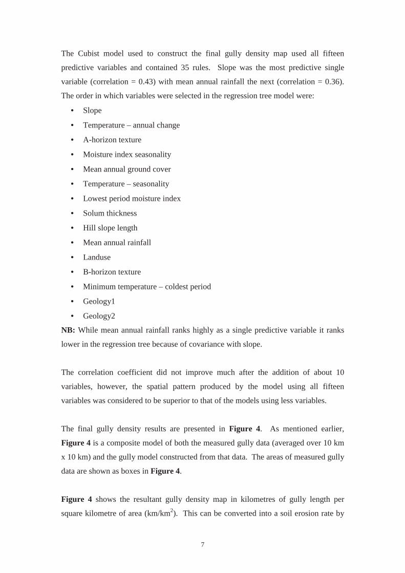
The final gully density results are presented in Figure 4. As mentioned earlier,

Figure 4 is a composite model of both the measured gully data (averaged over 10 km

x 10 km) and the gully model constructed from that data. The areas of measured gully

data are shown as boxes in Figure 4.

Figure 4 shows the resultant gully density map in kilometres of gully length per

square kilometre of area (km/km2). This can be converted into a soil erosion rate by

8

considering the volume of soil removed to form a gully and its approximate age.

From available studies it was found that gullies have an average cross-sectional area

of 10m2. One kilometre of gully would then produce 10,000 cubic metres

(approximately 15 000 tonnes) of sediment per km2 of land. If that was eroded over a

typical gully age of 100 years, the mean annual rate of erosion would be 1.5

tonnes/hectare/year.

Figure 4 Composite gully density map for the Murray-Darling Basin (10 km x 10km

grid cells).

Figure 4 shows that some of the highest gully densities in the catchment occur on the

eastern rim. Much of this area was subject to early European settlement and gullies

9

developed late in the 19th C. These gullies continue to contribute fine sediment and

poor quality water, although gully expansion is largely complete (Eyles, 1977). The

high gully densities in this area are not unexpected due to the extent of land clearance

and intensive land use that have taken place. This area also consists of large areas of

erodible granitic-based soils on sloping land in a climate that leads to periods of low

ground cover.

Another area of moderate to high gully density is in the southern (Victorian) part of

the basin. This area was also subjected to early European settlement, particularly gold

mining of the 1850s. This combined with physiographic factors such as slope and

climate produced a zone of particularly high gully densities.

The other area of moderate to high gully density is in the area of the Mt Lofty Ranges,

South Australia. This area is similar in terrain, land use and climate to the areas of

high gully erosion density in the south-eastern parts of the basin. Interestingly this

area of moderate to high gully density was predicted solely by the model as there were

no measured gullies in this region. Some checking against aerial photographs from

this region confirms that it is an area of moderate to high gully density.

There is little gully erosion predicted over the central and north-western parts of the

basin. Much of this region is far from areas of measured gully erosion and the

modelling is thus an extrapolation. We have confidence in the results because they

compare favourably with the 1988 reconnaissance-scale survey of land degradation in

New South Wales (Graham, 1989) which did map those areas. This mapping, at a

coarser resolution, and our modelling both show very little gully erosion where

rainfall and slope decreased. Therefore any errors in the extrapolation have little

consequence for our sediment budgets. There is no gully erosion mapping for

Queensland but much of that region has similar environmental conditions to northern

and western New South Wales so the modelling is not being used to make long

extrapolations, giving some confidence in the results.

Overall, the average gully density for the MDB is 0.08 km/km2. There are

approximately 89,000 km of gully in total, which on average have produced 13

million tonnes of sediment per year. In total, gullies in the MDB have eroded 1.3

10

billion tonnes of sediment in historical times. The gully density predicted in this

report is less than that predicted by the NLWRA gully density model (0.13 km/km2).

We attribute this result to the use of higher quality input data and the consequent

generation of more accurate spatial models.

1.4 Time Sequence of Gully Erosion

The river sediment budget model (SedNet) produces mean annual river loads from a

mass balance of mean annual rates of sediment input and deposition. As described

above, the basic measurement of gully density is converted into a mean annual rate of

sediment supply by dividing the total volume of gullies by their age. This produces

the time averaged rate of sediment supply. If we interpret those results as

representing the current state of sediment transport in the basin we are implicitly

assuming that there are no strong temporal patterns in the development of gullies over

historical times. That is, we assume that the time-averaged sediment yield from

gullies is a reasonable approximation of the current sediment yield, considering the

degree of uncertainty in the other aspects of the modelling. For the NLWRA, a

constant value of gully age of 100 y was used across the assessment area. Here we

consider whether an improved representation of time in the gully modelling is

justified.

Early work on the historical development of gully erosion focussed on the Southern

Tablelands of New South Wales, mainly to the south of Canberra (Eyles, 1977;

Prosser and Winchester, 1996). This work showed that the majority of present gullies

were initiated soon after settlement of the region and associated clearing of forests and

degradation of valley-floor vegetation. The historical documentary and field evidence

shows that most gullies formed between 1850 and 1900. Aerial photography first

became available in the 1940’s. Comparison of gully extent on those photographs

with the current photographs showed very little change in gully extent in the last 50

years. This history of gully development has been used to suggest that gully sediment

yields were very high from 1850 to 1900, declining in time since that date. The

current rate of erosion remains uncertain, however. It should also be noted though

that the vast bulk of sediment yielded from gullies is derived from the sidewalls rather

11

than the gully head (Blong et al., 1982) so that stability of gully extent since the

1940’s does not necessarily imply a reduction in sediment yield.

A similar history of gully erosion has been found for the Victorian part of the MDB,

where gold mining, beginning around the 1850’s was an additional cause of

widespread gully development. For the Southern Tablelands of New South Wales and

Victoria there is clear evidence that the sediment yields of gullies should be averaged

over 150 y rather than 100 y. We have undertaken high resolution SedNet predictions

in the Goulburn-Broken catchment of Victoria and compared these to results of water

quality monitoring at 11 stations across the catchment. The monitoring results

provide a good estimate of current sediment yield, and the monitored sites cover a

wide range of gullied and un-gullied sub-catchments. There is a strong association of

high area specific sediment yield (t/ha/y) recorded at the monitoring stations and the

total extent of gully erosion upstream. All stations with high sediment yields come

from sub-catchments with moderate to high gully densities. This suggests that gullies

still yield considerable sediment today, despite the drier than average conditions over

the monitoring period and the age of the gullies. The SedNet model predicts that

across the Goulburn-Broken catchment, gullies are responsible for 60% of the total

sediment yield. The current sediment yield is systematically over-predicted, in

comparison with gauging stations, if the mean annual yield from gullies is estimated

using an age of 100 y. Predictions are close to observations if a gully age of 150 is

used. The results suggest that specifying gully age may improve the results but that

no further inclusion of temporal patterns is warranted, given the uncertainty over these

patterns as outlined below.

More recent work on the history of erosion has expanded the geographical scope of

the studies beyond the Southern Tablelands and into other regions, although still

focussed in the south eastern part of the basin. This has shown that the majority of

gully erosion, and riverbank erosion, does not always occur immediately after initial

agricultural settlement. In Tarcutta Creek, a tributary of the middle Murrumbidgee

catchment, Page and Yarden (1998) found that gullies and stream banks expanded as

late as the 1980’s. We have found anecdotal evidence for widespread gully initiation

in the nearby Tumut River catchment in the 1960’s. A detailed study of a highly

eroded sub-catchment of the Lachlan River (Bush, 2001) found that one third of the

12

gully length formed between 1944 and the present day. Work on a grazed savannah

catchment in Queensland found that while there were extensive gullies present in

1960 they doubled in length between then and the present day, despite no further land

clearing (Post, unpublished data). The reasons for the differences between these

regions and the Southern Tablelands of New South Wales are not yet clear and until

further information is available it is hard to justify moving away from a time averaged

gully sediment yield to gully growth as a function of time.

2 Introduction to Riverbank Erosion

Riverbank erosion is the most uncertain of the sediment source terms in the river

budget modelling. It is known that degradation of riparian vegetation and other

impacts on our rivers have resulted in greatly increased rates of riverbank erosion, to

the extent that this erosion process cannot be ignored as a sediment source in regional

assessments. There remains, however, very little data on the rates of river bank

erosion and the environmental factors controlling those rates. The only large-scale

quantitative rule of which we are aware is the simple empirical rule for meander

migration and bank erosion proposed by Rutherfurd (2000) following a review of

global literature:

60.058.1016.0 QBE = (1)

where BE is the bank erosion rate in metres of recession per year, and Q1.58 is the

discharge (m3/s) of the 1.58 y recurrence interval flood event, assumed to represent

bankfull discharge. The bank rule essentially scales the rate of bank erosion to the

size of the river as both size and discharge increase with catchment area. This rule

was applied across Australia as part of the river sediment budgets for the NLWRA.

The results revealed two limitations. First, many of the highest predicted rates of

bank erosion were in high discharge rivers that were largely undisturbed with

resultant low rates of bank erosion. Brooks (1999) has shown that natural rates of

bank erosion can be very low in Australian rivers with intact riparian vegetation and

that erosion is greatly accelerated with removal of riparian vegetation (see also

Abernethy and Rutherfurd, 2000; Prosser et al. 2001). Second, the overall rate of

erosion was too high when averaged over historical times, contributing more sediment

13

to rivers than recorded by river monitoring data. Equation (1) was modified for

inclusion in SedNet to incorporate these three effects:

( )( ) 60.058..11008.0 QPRBE xx −= . (2)

where PRx is the proportion of bank with intact native riparian vegetation. Riparian

vegetation was mapped across the NLWRA assessment area, including the MDB, by

intersection of the river network with a grid of native vegetation cover detected by

remote sensing in 1995. This was obtained from the Australian Land Cover Change

project at a resolution of 100 m (BRS, 2000). This is the best available data but is

still a crude measure of riparian condition. The 100 m resolution fails to identify

narrow bands of remnant riparian vegetation in cleared areas but it also fails to

identify narrow valleys of cleared land penetrating otherwise uncleared land.

For sediment budgets, the erosion rate needs to be expressed in terms of tonnes per

year of sediment eroded along the length (Lx, m) of each river link x. We did this by

assuming a mean bank height of 3 m, and a sediment bulk density of 1.5 t/m3. Thus

( )( ) xx LQPRBC 6.058.1118 −= (3)

where BCx is the input from bank erosion in each link (t/y).

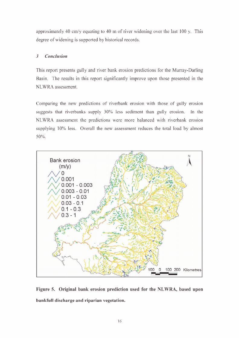
The results of bank erosion mapping for the MDB, using equation (2) are shown in

Figure 5. These are the results included in the NLWRA assessment. Geomorphic

studies of our lowland rivers show that they have experienced very little historical

erosion (Rutherfurd, 2000), and in some areas there is greater concern over channel

contraction rather than erosion. This observed pattern is not reflected in the results of

Figure 5, because Equation 2 predicts an ever increasing rate of bank erosion as a

river increases in size and discharge downstream. This is particularly evident along

the Darling River where very high rates of erosion are predicted along cleared river

banks.

2.1 MDB Assessment of Riverbank Erosion

The main processes of riverbank erosion are mass failure of the banks (slumping) and

scour of the banks by the hydraulic forces of flow. Mass failure results in local

14

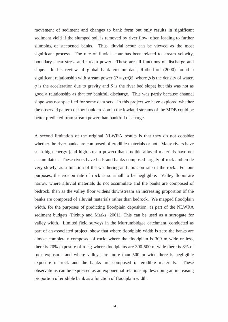
movement of sediment and changes to bank form but only results in significant

sediment yield if the slumped soil is removed by river flow, often leading to further

slumping of steepened banks. Thus, fluvial scour can be viewed as the most

significant process. The rate of fluvial scour has been related to stream velocity,

boundary shear stress and stream power. These are all functions of discharge and

slope. In his review of global bank erosion data, Rutherfurd (2000) found a

significant relationship with stream power (P = ρgQS, where ρ is the density of water,

g is the acceleration due to gravity and S is the river bed slope) but this was not as

good a relationship as that for bankfull discharge. This was partly because channel

slope was not specified for some data sets. In this project we have explored whether

the observed pattern of low bank erosion in the lowland streams of the MDB could be

better predicted from stream power than bankfull discharge.

A second limitation of the original NLWRA results is that they do not consider

whether the river banks are composed of erodible materials or not. Many rivers have

such high energy (and high stream power) that erodible alluvial materials have not

accumulated. These rivers have beds and banks composed largely of rock and erode

very slowly, as a function of the weathering and abrasion rate of the rock. For our

purposes, the erosion rate of rock is so small to be negligible. Valley floors are

narrow where alluvial materials do not accumulate and the banks are composed of

bedrock, then as the valley floor widens downstream an increasing proportion of the

banks are composed of alluvial materials rather than bedrock. We mapped floodplain

width, for the purposes of predicting floodplain deposition, as part of the NLWRA

sediment budgets (Pickup and Marks, 2001). This can be used as a surrogate for

valley width. Limited field surveys in the Murrumbidgee catchment, conducted as

part of an associated project, show that where floodplain width is zero the banks are

almost completely composed of rock; where the floodplain is 300 m wide or less,

there is 20% exposure of rock; where floodplains are 300-500 m wide there is 8% of

rock exposure; and where valleys are more than 500 m wide there is negligible

exposure of rock and the banks are composed of erodible materials. These

observations can be expressed as an exponential relationship describing an increasing

proportion of erodible bank as a function of floodplain width.

15

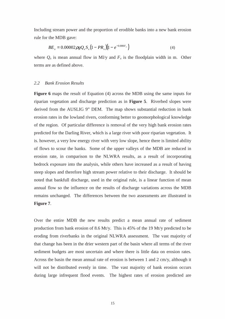
Including stream power and the proportion of erodible banks into a new bank erosion

rule for the MDB gave:

( )( )xFxxxx ePRSgQBE 008.01100002.0 −−−= ρ (4)

where Qx is mean annual flow in Ml/y and Fx is the floodplain width in m. Other

terms are as defined above.

2.2 Bank Erosion Results

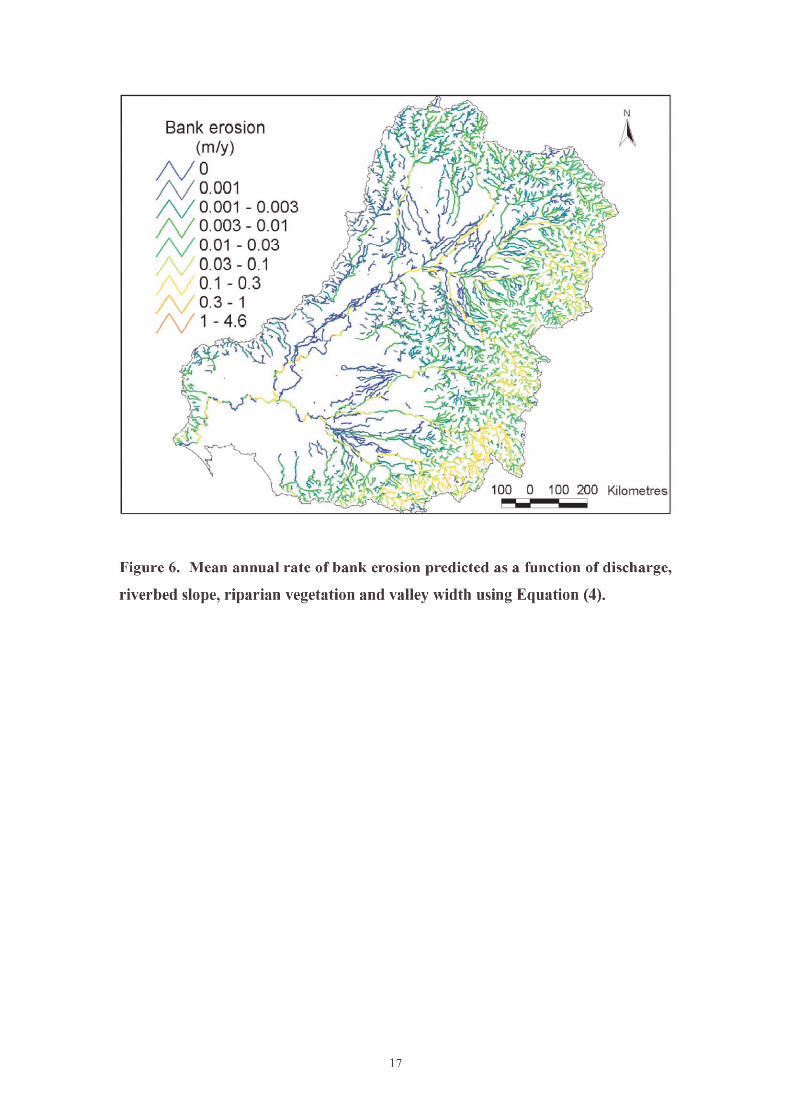
Figure 6 maps the result of Equation (4) across the MDB using the same inputs for

riparian vegetation and discharge prediction as in Figure 5. Riverbed slopes were

derived from the AUSLIG 9” DEM. The map shows substantial reduction in bank

erosion rates in the lowland rivers, conforming better to geomorphological knowledge

of the region. Of particular difference is removal of the very high bank erosion rates

predicted for the Darling River, which is a large river with poor riparian vegetation. It

is. however, a very low energy river with very low slope, hence there is limited ability

of flows to scour the banks. Some of the upper valleys of the MDB are reduced in

erosion rate, in comparison to the NLWRA results, as a result of incorporating

bedrock exposure into the analysis, while others have increased as a result of having

steep slopes and therefore high stream power relative to their discharge. It should be

noted that bankfull discharge, used in the original rule, is a linear function of mean

annual flow so the influence on the results of discharge variations across the MDB

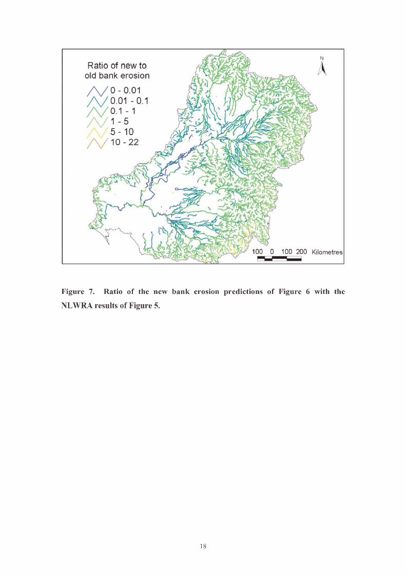
remains unchanged. The differences between the two assessments are illustrated in

Figure 7.

Over the entire MDB the new results predict a mean annual rate of sediment

production from bank erosion of 8.6 Mt/y. This is 45% of the 19 Mt/y predicted to be

eroding from riverbanks in the original NLWRA assessment. The vast majority of

that change has been in the drier western part of the basin where all terms of the river

sediment budgets are most uncertain and where there is little data on erosion rates.

Across the basin the mean annual rate of erosion is between 1 and 2 cm/y, although it

will not be distributed evenly in time. The vast majority of bank erosion occurs

during large infrequent flood events. The highest rates of erosion predicted are

19

4 References Abernethy, B. and I.D. Rutherfurd. (2000). "The effect of riparian tree roots on

riverbank stability." Earth Surface Processes and Landforms. 25, 921-937.

Blong, R. J., Graham, O. P. Veness J. A. (1982). “The role of sidewall processes in

gully development”, Earth Surface Processes and Landforms 7, 381-385.

Brooks, A. (1999), "Lessons for river managers from the fluvial tardis." In I.D.

Rutherfurd and R. Bartley, editors, Second Australian Stream Management

Conference: The Challenge of Rehabilitating Australia's Streams.

Cooperative Research Centre for Catchment Hydrology. Melbourne.121-128.

BRS, 2000. http://www.brs.gov.au:80/land&water/landcov/alcc_results.html

Bush, L. (2001). “Time, Space and Causality: Gully Erosion in Milburn Creek

Catchment, Central Western New South Wales”. BSc Hons. Thesis,

Australian Defence Force Academy, University of New South Wales,

Canberra.

Eyles, R.J. (1977). “Changes in drainage networks since 1820, Southern Tablelands,

NSW”, Australian Geographer, 13, 377-387.

Ford, G.W., Martin, J.J., Rengasamy, P., Boucher, S.C., Ellington, A. (1993). “Soil

Sodicity in Victoria”, Australian Journal of Soil Research, 31, 869-909.

Galloway, J. N, Howarth, R. W., Michaels, A. F., Nixon, S. W., Prospero, J. M., and

Dentener, F. (1996) “Nitrogen and phosphorus budgets of the North Atlantic

Ocean and its watershed.” Biogeochemistry, 35, 3-25.

Graham, O.P. (1989). “Land degradation survey of NSW 1987-88: Methodology”.

SCS Technical Report No. 7 Soil Conservation Service of New South Wales.

Lemly, A. D. (1982) “Modification of benthic insect communities in polluted streams:

combined effects of sedimentation and nutrient enrichment”, Hydrobiologia,

87, 229-245.

Olley, J.M., Murray, A.S., Mackenzie, D.M., Edwards, K. (1993) “Identifying

sediment sources in a gullied catchment using natural and anthropogenic

radioactivity.” Water Resources Research, 29, 1037-1043.

Page, K.J., Yarden, Y.R. (1998). “Channel adjustment following the crossing of a

threshold: Tarcutta Creek, South Eastern Australia.” Australian Geographical

Studies, 36, 289-311.

Pickup, G., Marks, A. (2001). “Identification of floodplains and estimation of

20

floodplain flow velocities for sediment transport modelling.” Technical Report

14/01, CSIRO Land and Water, Canberra.

Prosser, I.P., Winchester, S.J. (1996) “History and processes of gully initiation and

development in Australia.” Zeitschrift für Geomorphologie Supplement Band,

105, 91-109.

Prosser, I.P., I.D. Rutherfurd, J. Olley, W.J. Young, P.J. Wallbrink, and C.J. Moran.

(2001), "Large-scale patterns of erosion and sediment transport in river

networks, with examples from Australia." Marine and Freshwater Research.

52, 81-99.

Rulequest Research (2002). “Data mining with Cubist”,

http://www.rulequest.com/cubist-info.html

Rutherfurd, I. (2000), “Some human impacts on Australian stream channel

morphology”. In Brizga, S. and Finlayson, B. River Management: The

Australasian Experience. Chichester, John Wiley & Sons, 2-52.

Wallbrink, P.J., Murray, A.S., Olley, J.M., Olive, L.J. (1998) “Determining sources

and transit times of suspended sediment in the Murrumbidgee River, New

South Wales, Australia, using fallout 137Cs and 210Pb. Water Resources

Research, 34, 879-887.

Wasson R.J, Mazari R.K, Starr B, Clifton G. (1998). “The recent history of erosion

and sedimentation on the Southern tablelands of southeastern Australia:

sediment flux dominated by channel incision.” Geomorphology, 24, 291-308.