gum analysis for tims and sims isotopic ratios in graphite · pnnl-17036 . gum analysis for tims...

PNNL-17036

GUM Analysis for TIMS and SIMS Isotopic Ratios in Graphite PG Heasler JB Cliff DC Gerlach SL Petersen April 2007 Prepared for the U.S. Department of Energy under Contract DE-AC05-76RL01830

DISCLAIMER

This report was prepared as an account of work sponsored by an agency of the

United States Government. Neither the United States Government nor any

agency thereof, nor Battelle Memorial Institute, nor any of their employees,

makes any warranty, express or implied, or assumes any legal liability or

responsibility for the accuracy, completeness, or usefulness of any

information, apparatus, product, or process disclosed, or represents that

its use would not infringe privately owned rights. Reference herein to any

specific commercial product, process, or service by trade name, trademark,

manufacturer, or otherwise does not necessarily constitute or imply its

endorsement, recommendation, or favoring by the United States Government

or any agency thereof, or Battelle Memorial Institute. The views and opinions

of authors expressed herein do not necessarily state or reflect those of the

United States Government or any agency thereof.

PACIFIC NORTHWEST NATIONAL LABORATORY

operated by

BATTELLE

for the

UNITED STATES DEPARTMENT OF ENERGY

under Contract DE-AC05-76RL01830

Printed in the United States of America

Available to DOE and DOE contractors from the

Office of Scientific and Technical Information,

P.O. Box 62, Oak Ridge, TN 37831-0062;

ph: (865) 576-8401

fax: (865) 576-5728

email: [email protected]

Available to the public from the National Technical Information Service,

U.S. Department of Commerce, 5285 Port Royal Rd., Springfield, VA 22161

ph: (800) 553-6847

fax: (703) 605-6900

email: [email protected]

online ordering: http://www.ntis.gov/ordering.htm

This document was printed on recycled paper.

(8/00)

PNNL-17036

GUM Analysis for TIMS and SIMS Isotopic Ratios

in Graphite

P. G. Heasler

D. C. Gerlach

J. B. Cliff

S. L. Petersen

April 2007

Prepared for

the U.S. Department of Energy

under Contract DE-AC05-76RL01830

Pacific Northwest National Laboratory

Richland, Washington 99352

iii

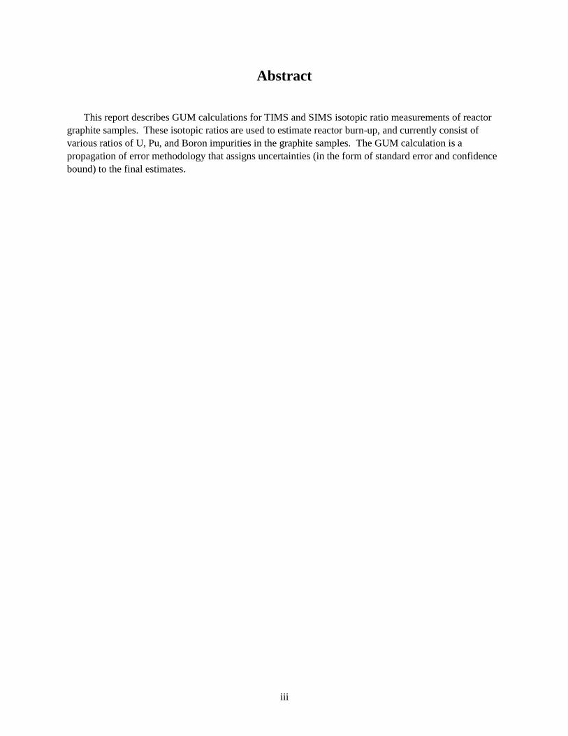
Abstract

This report describes GUM calculations for TIMS and SIMS isotopic ratio measurements of reactor

graphite samples. These isotopic ratios are used to estimate reactor burn-up, and currently consist of

various ratios of U, Pu, and Boron impurities in the graphite samples. The GUM calculation is a

propagation of error methodology that assigns uncertainties (in the form of standard error and confidence

bound) to the final estimates.

v

Contents

Abstract ........................................................................................................................................................ iii

Glossary ...................................................................................................................................................... vii

1.0 Overview of GUM ............................................................................................................................. 1.1

2.0 SIMS Measurements .......................................................................................................................... 2.1

2.1 Sample Preparation and Storage for SIMS Analysis ................................................................ 2.1

2.2 Contamination Control .............................................................................................................. 2.1

2.3 Analyses .................................................................................................................................... 2.1

2.4 Standards ................................................................................................................................... 2.2

2.5 Results ....................................................................................................................................... 2.2

2.6 Estimation Procedure ................................................................................................................ 2.5

2.6.1 Step 1: Gross Measurement Corrections .................................................................. 2.5

2.6.2 Step 2: ANOVA Analysis ........................................................................................ 2.5

2.6.3 Step 3: Final Estimates ............................................................................................. 2.7

2.7 Results from BEPO Test Samples ............................................................................................ 2.8

2.8 August 2006 Qualification Sample Results ............................................................................ 2.13

2.8.1 Results for Sample QA-21353 Anova Results ........................................................ 2.14

2.8.2 Results for Sample QA-21361, ANOVA Results ................................................... 2.14

2.8.3 Results for Sample QA-27277, Anova Results ....................................................... 2.15

2.8.4 Day-to-Day Variability Study ................................................................................. 2.15

2.8.5 GUM Tables for Qualification samples .................................................................. 2.16

3.0 TIMS Measurements .......................................................................................................................... 3.1

3.1 Samples for TIMS Analyses, Preparation and Processing ........................................................ 3.1

3.2 TIMS Blanks ............................................................................................................................. 3.5

3.3 Uranium Reference Standard Results ....................................................................................... 3.8

3.4 TIMS Estimation Procedure...................................................................................................... 3.9

3.4.1 Step 1: Calculate Corrected Count Rates ............................................................... 3.10

3.4.2 Step 2: Calculate Atomic Ratios ............................................................................ 3.10

3.4.3 Step 3: Calculate Means ......................................................................................... 3.11

3.4.4 Step 4: Correct Means for Bias .............................................................................. 3.11

3.5 GUM Version of Estimation Procedure for TIMS data .......................................................... 3.11

3.6 August 2006 Qualification Sample Results ............................................................................ 3.12

4.0 References .......................................................................................................................................... 4.1

Appendix A – GUM Tables for All TIMS Analyses of NBL BEPO Sample and

NBL Qualification Samples .............................................................................................................. A.1

vi

Tables

1 Format of a GUM Uncertainty Table ............................................................................................... 1.2

2 Results for Mass Bias Calibration .................................................................................................... 2.3

3 Results for Day-to-Day Variability Study ........................................................................................ 2.3

4 Results for Sample QA-21361 ......................................................................................................... 2.3



7 Results from ANOVA Analysis of SIMS Data ................................................................................ 2.7

8 Correlations from ANOVA Analysis of SIMS Data ........................................................................ 2.7

9 GUM Results for BEPO Sample 28402 ........................................................................................... 2.9

10 GUM Results for BEPO Sample 37796 ......................................................................................... 2.10

11 GUM Results for BEPO Sample 44746 ......................................................................................... 2.11

12 ANOVA Results from BEPO Samples .......................................................................................... 2.12

13 GUM Table for Qualification Sample 21353 SIMS Results .......................................................... 2.16



16 Uranium TIMS Results for NBL BEPO Samples ............................................................................ 3.3

17 Plutonium TIMS Results for NBL BEPO Samples ......................................................................... 3.3

18 Uranium TIMS Results for NBL QA Samples ................................................................................ 3.4

19 Plutonium TIMS Results for NBL QA Samples .............................................................................. 3.4

20 Uranium Contents and Isotope Ratios in Blank Graphite and Sample Processing Blanks .............. 3.6

21 Plutonium Contents and Isotope Ratios in Blank Graphite and Sample Processing Blanks ............ 3.7

22 Compilation of Results for NBS 950s Natural U Standard .............................................................. 3.8

23 Typical Uncertainties for Pu Estimates of BEPO Sample Ratios

Pu240/Pu239, Pu241/Pu239, and Pu242/Pu239 ............................................................................ 3.12

24 Correlation Table for Pu Ratios ..................................................................................................... 3.12

25 Empirical vs. POE RE .................................................................................................................... 3.12

26 Calibration Parameter Table for Sample 84104 ............................................................................. 3.13

27 Example of Corrected Count-Rate Table for Sample 84104, Based on

Interpolated Count Rates Supplied by PNNL TIMS Data Reduction Program ............................. 3.14

28 GUM Relationship between Total Ion Counts for Mass 239 and

Preceding Data Inputs (Table 26 and Table 27). ............................................................................ 3.14

29 Pu GUM Tables for Sample 84104 ................................................................................................ 3.15

vii

Glossary

CR A corrected count rate (particles per second). This is corrected for instrument biases.

GCR A gross count rate (particles per second). This is the measurement the instrument

produces.

GRM9,GRM10,GRM11,GRM13 Gross count rates (counts per sec) of various AMUs.

GUM Guide quantifying Uncertainty in analytic Measurements

NLB New Brunswick Laboratory

PPMB, PPMBe PPM concentration (atomic) of boron and beryllium in the sample. These two quantities

are also end-products of the analysis.

R Identifies an isotopic ratio

R10Be/9Be This is the isotopic ratio of Be produced by nuclear reactions as the reactor operates.

This quantity is not measured, but calculated with a reactor code and is approximately

1/45.

R13C/C Abundance of

13C in graphite (.012). This is not measured, but obtained from reference.

RB10/B11 Ratio (atomic) of 10

B to 11

B in the sample. This is the central quantity to be estimated for

the sample. It is corrected for 10

Be contamination.

RDEB10/B11 Relative detector efficiency of 10

B versus 11

B atoms. This correction factor is determined

by measurements on Brookhaven standards. And describes mass bias for the detector.

RDF Relative Detection Efficiency Factor

RM9/M10, RM10/M11, RM11/M13 Ratios of M9/M10, M10/M11, and M11/M13 particles in the sample.

RSF Relative Sensitivity Factor

RSFB/C Relative sensitivity factor for boron versus carbon. This correction factor is determined

by measuring a standard with the instrument.

RSFBe/C Relative sensitivity factor for beryllium versus carbon. This is also determined by

measurements on a standard.

SIMS Secondary Ionization Mass Spectrometry

TIMS Thermal Ionization Mass Spectrometry

1.1

1.0 Overview of GUM

The section provides a brief summary of the GUM methodology with a description of the tables

produced. GUM is basically a propagation of error calculation, with a GUM table presenting some terms

in the POE calculation for diagnostic evaluation.

Let us suppose the vector x = (x1, x2, ..., xn)T represents the raw input data (and calibration parameters)

from a chemical analysis, and y = (y1, y2, ..., yp)T the final estimates produced by the chemical analysis,

using an estimation procedure described by the function F (∙). In other words, the estimation procedure is

ˆ ˆy F x (1)

Most typically, the estimation procedure is derived from a formula that relates the “true values” x and y to

each other (i.e., y = F(x)). As an example, for mass spectrograph measurements, the input vector, x would

include raw counts of various atomic mass units of interest, and y would consist of desired isotopic ratios.

From this overview, propagation of errors is easy to explain. The input variable, x is assumed to be a

random vector, with uncertainty(a)

defined by its covariance matrix ˆCov x . The uncertainty of the final

estimate, y, is described by its covariance, which is approximated by the POE formula

Tˆ ˆCov y dFCov x dF (2)

where dF represents the differential of F with respect to x. dF is a p × n matrix, with element ij

representing the derivative dyi/dxj. The GUM uncertainty calculation uses this formula to calculate

ˆCov y as the basis for estimate uncertainty.

However, another quantity is also required to describe the uncertainty in y for GUM – its degrees of

freedom, represented as dof (y). The degrees of freedom are used to produce approximate confidence

intervals on y. Thus, in GUM calculations, uncertainty is described by a covariance matrix and a degrees

of freedom vector. This requires that a degrees of freedom vector, dof(x), must be supplied for the inputs.

Any component in x that is the result of replicated measurements will have a dof associated with it

(number of replicates minus 1). Generally, dof(xi) describes how much data was used to determine ix and

iˆCov x . The degrees of freedom associated with y is calculated with Saiterwait’s approximation, and is

given by

4

1 1

1

nik

k ii ki

sd xdydo f y do f x

dx sd y

(3)

The GUM uncertainty calculation, as represented by Eqs. 1, 2, and 3, is organized into a Gum

Uncertainty Table, as illustrated in Table 1. The top half of the table contains the inputs to the calculation

(a) When x represents a single value, Cov(x) = Var(x).

1.2

(i.e., x) and the last line contains the uncertainty associated with the output, yk. The right-hand side of the

table contains intermediate values that can be used as diagnostics. Below the table is a description of the

table diagnostics;

Table 1. Format of a GUM Uncertainty Table

Variable Estimate

Standard

Error (SE) DOF

Sensitivity

Factor

Uncertainty

Contrib.

% Tot.

Var. Index

x1 1x 1ˆsd x 1ˆdo f x dyk/dx1 U1 I1



. . . . . . .

. . . . . . .

. . . . . . .

xn nx nˆsd x nˆdo f x dyk/dxn Un In

Result yk ky kˆsd y kˆdo f y

Sensitivity Factor: This is the derivative dyk/dxi (also element k, i in the matrix dF) and represents the

rate of change of variable yk to xi.

Uncertainty Contribution: This is the standard error times the sensitivity factor and represents the

standard error we would see in the result if xi were the only source of uncertainty.

i i iU = dy/dx · sd(x ) (4)

Index: This is the % contribution of variable xi to the total variance in the result.

2

100 ii

UI

sd( y )

(5)

It is sometimes more useful to replace the standard error column in the GUM table with Relative

Error (RE). Relative error is defined as

100ˆsd x

ˆRE xx

(6)

Note that relative error is expressed as a percentage. The GUM tables presented in this report use

relative error instead of standard error.

2.1

2.0 SIMS Measurements

2.1 Sample Preparation and Storage for SIMS Analysis

Upon arrival at PNNL, the three samples QA-21353, QA-27277, and QA-21361 were removed from

the packaging and put into air-tight Teflon containers for storage. After visual inspection, samples

QA-27277 and QA-21361 were deemed appropriate for analysis based on having acceptable dimensions

for fitting into the SIMS sample holder and having one flat surface. Neither side of sample QA-21353

was deemed to be acceptable for analysis. The best side had saw chatter and a ridge that would have

prohibited having a level analysis surface in the sample holder. A razorblade that had been cleaned by

sequential sonication in distilled, deionized water, acetone, and methanol was used to remove the ridge so

that the sample could fit with the best possible orientation in the sample holder. Despite this

modification, sample QA-21353 was less than optimum for SIMS analysis due to the saw chatter and the

fact that the surface was not flat over the entire diameter of the sample.

2.2 Contamination Control

The SIMS at PNNL is equipped with a four-aperture, multiple-immersion lens strip. One of these

apertures has been dedicated to B analyses for the GIRM project. A single sample holder was used for

these samples. The sample holder and forceps used to manipulate the samples were sonicated

sequentially in deionized water, acetone, and methanol between samples. To remove airborne

contamination, each analysis location was presputtered for two minutes with a stationary, 1 µA beam,

defocused to ~250 µm.

2.3 Analyses

For all analyses, an 8 keV O2+ primary beam was used. The 150 µm transfer lens was used with an

400 µm contrast diaphragm and 1800 µm field aperture. The exit slit was wide open, the energy slit was

centered and closed to an energy width of 10 eV (FWHM). The entrance slit was closed to allow about

50%–70% transmission of secondary ions. For most analyses, 102 data cycles were acquired. The first

cycle was discarded and the remaining 101 were automatically interpolated using the Charles Evans

software. After the presputter phase, the primary beam was adjusted so that the 11

B signal was about

104 cts s

-1. The count ratio between

10B and

11B varied between samples so that for sample QA-21353,

10B was counted for 4 seconds and

11B was counted for 2 seconds per cycle. For QA-27277,

10B was

counted for 6 seconds and 11

B for 2 seconds per cycle, and for sample QA-21361, 10

B was counted for

8 seconds and 11

B for 2 seconds per cycle.

Two types of analyses were performed on the QA samples (QA-21353, QA-27277, and QA-21361).

In the first type, the three samples were analyzed three different times each over the course of nearly two

months. Since the instrument was used for a wide variety of analyses between analyzing the GIRM QA

samples, these analyses not only capture, analysis-to-analysis, spot-to-spot, and day-to-day variability,

they also capture variability induced from retuning the instrument, reorienting the sample in the holder,

aging of the electronics, etc. In these analyses, a sample was placed into the sample holder with a random

orientation. A spot was chosen at X = 0 mm, and Y = –2 mm on the stage axis. The sample was

sputtered with an approximately 1 uA stationary beam for two minutes with the beam defocused to be

2.2

larger than the 150 µm FOV set by the field aperture (~ 250 µm). Three 102-cycle analytical runs were

performed on each spot. After the three analyses, the stage was moved 1 mm in the positive Y direction

and the analysis cycle was repeated for a total of five spots. These analyses were repeated three times; on

June 2–5, June 7–8, and July 24–26.

The second type of analysis was performed on sample QA-21353 and was designed to test day-to-day

variation on the same spot as directed by the steering committee. Five spots were chosen at the X,Y

coordinates (-1,0), (0,0), (1,0), (0,-1), and (0,1). The RAE imaging detector was employed in order to

find the same spot from day to day. This turned out to be advantageous as there was some discrepancy

observed in loading the sample holder from day to day when relying solely on the stage position

micrometers. Thus, five spots were analyzed using the same protocol as above (except that only

52 cycles were recorded instead of 102) on three separate days. The sample holder was removed from the

instrument daily and replaced. The samples were not removed from the sample holder each day and re-

inserted, however – this would have caused difficulties in relocating the same spots for analysis. The

same analysis spots were located by comparing the 11

B ion image with a reference image saved from

day 1.

2.4 Standards

Standards VA3, VB3, and VC3 were analyzed six different times over the time period from

October 7, 2005, to May 26, 2006. In these analyses conducted over a relatively long period of time, the

standards were removed from the sample holder each time, and no attempt was made to relocate the same

spots for repeat analyses. Each standard was analyzed with a similar protocol as the QA samples; i.e., an

area was presputtered for 1–2 minutes with a 1-uA stationary beam, followed by analyses of five spots per

standard with three analytical runs consisting of 102 cycles per spot. For standard VA3, 10

B was counted

for 4 seconds and 11

B was counted for 2 seconds per cycle. For VB3, 10

B was counted for 6 seconds and 11

B for 2 seconds per cycle, and for standard VC3, 10

B was counted for 8 seconds and 11

B for 2 seconds

per cycle.

2.5 Results

Table 2 reports the results for the SIMS mass calibration standards (VA3, VB3, and VC3) at PNNL.

The mass bias estimate based on 270 individual measurements was 0.962 ± 0.011 (95% CI).

Table 3 reports the results for the day-to-day variability study in which the same five spots were

revisited on three consecutive days on the GIRM qualification sample QA-21353. Here relative errors on

the estimates for the contributions to are reported as well as if the contribution to the total uncertainty is

significantly different from zero. These data show that the day-to-day variability of sample QA-21353

was not a significant contributor to the error estimate when the same spots were analyzed on consecutive

days.

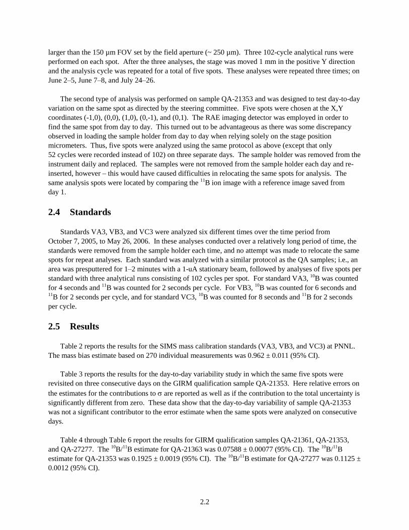
Table 4 through Table 6 report the results for GIRM qualification samples QA-21361, QA-21353,

and QA-27277. The 10

B/11

B estimate for QA-21363 was 0.07588 ± 0.00077 (95% CI). The 10

B/11

B

estimate for QA-21353 was 0.1925 ± 0.0019 (95% CI). The 10

B/11

B estimate for QA-27277 was 0.1125 ±

0.0012 (95% CI).

2.3

Table 2. Results for Mass Bias Calibration

Component DOF Value Relative Error (%)

X 2.84 0.9618 0.340

σstandard 2 5.18 10-3 54.5

σtime 5 2.38 10-3

58.7

σspot 72 8.37 10-3

8.0

σresidual 190 2.39 10-3

5.3

K(0.975, 2.84) = 3.28, X = 0.962 ± 0.011 (95% CI)

Table 3. Results for Day-to-Day Variability Study

Component DOF Value Relative Error (%) Significance

σday 2 2.28 10-4 86.9 No

σspot 4 4.49 10-4

47.0 No

σday dayt 8 3.62 10-4

36.7 Yes

σresidual 29 3.91 10-4

15.9

Table 4. Results for Sample QA-21361

Quantity

Nominal

Value

Relative

Error (%)

Effective

DOF

Uncertainty

Contribution Index (%) 10

B/11

B 0.0789 0.242 45.00 1.83 10-4

57.9

Mass Bias 0.9618 0.340 2.84 2.58 10-4

81.5

Result 0.0759 0.417 6.34

K(0.975, 6.34) = 2.42, X = 0.07588 ± 0.00077 (95% CI)


Quantity

Nominal

Value

Relative

Error (%)

Effective

DOF

Uncertainty


B/11

B 0.2001 0.233 49.60 4.49 10-4

56.6

Mass Bias 0.9618 0.340 2.84 6.54 10-4

82.4

Result 0.1925 0.412 6.08

K(0.975, 6.08) = 2.44, X = 0.1925 ± 0.0019 (95% CI)

2.4


Quantity

Nominal

Value

Relative

Error (%)

Effective

DOF

Uncertainty


B/11

B 0.1170 0.136 39.90 1.53 10-4

37.1

Mass Bias 0.9618 0.340 2.84 3.83 10-4

92.8

Result 0.1125 0.366 3.82

K(0.975, 3.82) = 2.83, X = 0.1125 ± 0.0012 (95% CI)

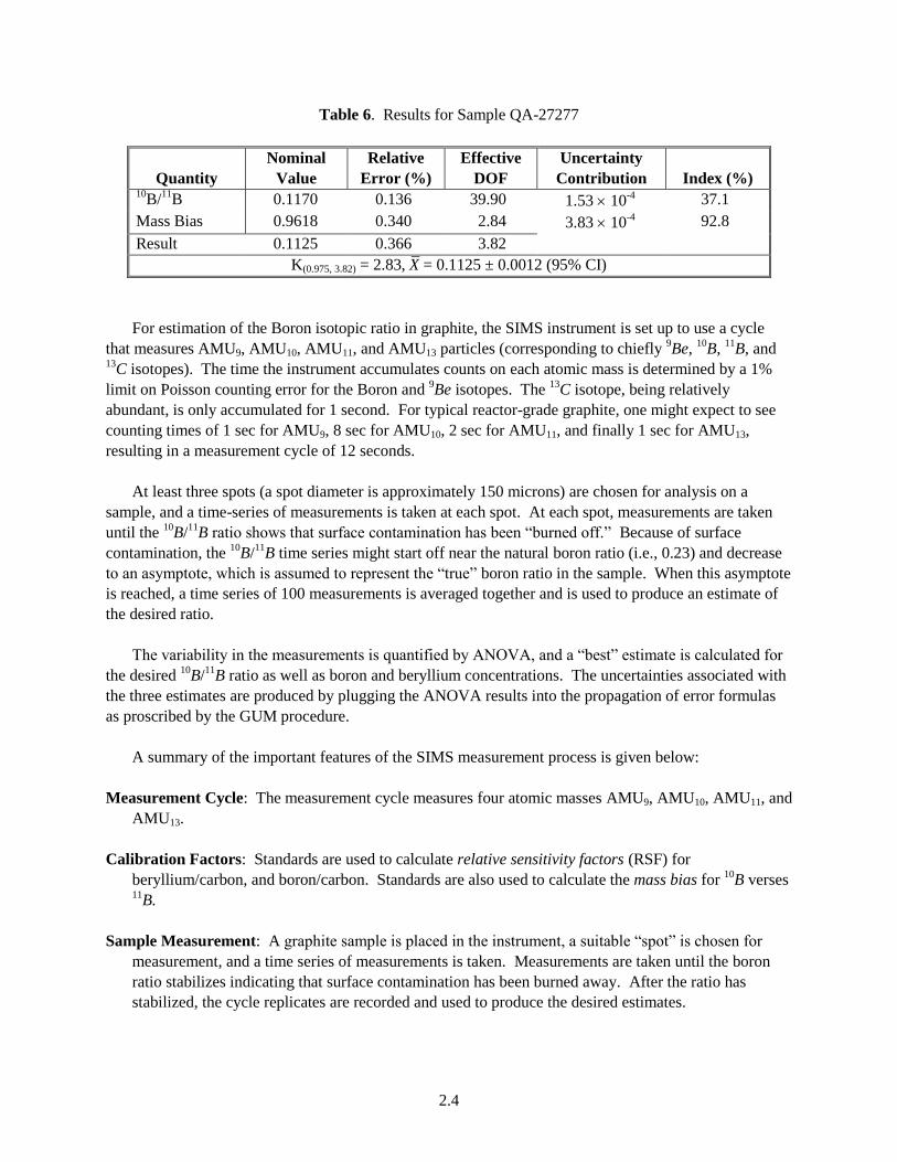
For estimation of the Boron isotopic ratio in graphite, the SIMS instrument is set up to use a cycle

that measures AMU9, AMU10, AMU11, and AMU13 particles (corresponding to chiefly 9Be,

10B,

11B, and

13C isotopes). The time the instrument accumulates counts on each atomic mass is determined by a 1%

limit on Poisson counting error for the Boron and 9Be isotopes. The

13C isotope, being relatively

abundant, is only accumulated for 1 second. For typical reactor-grade graphite, one might expect to see

counting times of 1 sec for AMU9, 8 sec for AMU10, 2 sec for AMU11, and finally 1 sec for AMU13,

resulting in a measurement cycle of 12 seconds.

At least three spots (a spot diameter is approximately 150 microns) are chosen for analysis on a

sample, and a time-series of measurements is taken at each spot. At each spot, measurements are taken

until the 10

B/11

B ratio shows that surface contamination has been “burned off.” Because of surface

contamination, the 10

B/11

B time series might start off near the natural boron ratio (i.e., 0.23) and decrease

to an asymptote, which is assumed to represent the “true” boron ratio in the sample. When this asymptote

is reached, a time series of 100 measurements is averaged together and is used to produce an estimate of

the desired ratio.

The variability in the measurements is quantified by ANOVA, and a “best” estimate is calculated for

the desired 10

B/11

B ratio as well as boron and beryllium concentrations. The uncertainties associated with

the three estimates are produced by plugging the ANOVA results into the propagation of error formulas

as proscribed by the GUM procedure.

A summary of the important features of the SIMS measurement process is given below:

Measurement Cycle: The measurement cycle measures four atomic masses AMU9, AMU10, AMU11, and

AMU13.

Calibration Factors: Standards are used to calculate relative sensitivity factors (RSF) for

beryllium/carbon, and boron/carbon. Standards are also used to calculate the mass bias for 10

B verses 11

B.

Sample Measurement: A graphite sample is placed in the instrument, a suitable “spot” is chosen for

measurement, and a time series of measurements is taken. Measurements are taken until the boron

ratio stabilizes indicating that surface contamination has been burned away. After the ratio has

stabilized, the cycle replicates are recorded and used to produce the desired estimates.

2.5

This measurement sequence is repeated at several spots on the sample. Measurement of more than

one spot allows one to calculate spot variability for the error analysis.

Calculation of Estimates: The sample measurements are combined to estimate the desired quantities and

the associated standard errors using the formulas described in this report.

2.6 Estimation Procedure

For purposes of description, we have organized the estimation procedure into three steps:

Step 1: Correct gross measurements for dead times and cycle bias.

Step 2: Estimate ratios and their variability with ANOVA.

Step 3: Calculate final estimates.

2.6.1 Step 1: Gross Measurement Corrections

Gross count rates, GR, are corrected for dead time and then interpolated. The dead-time correction

uses the standard formula

dtc exp = ( )GR GR GR (7)

where τ represents the instrument dead time. The error associated with this correction depends on the

uncertainty in the dead time. Given the count-rates used for these measurements, this uncertainty is

insignificant (with a RSD less than 10-4

) and is considered to be zero in the uncertainty calculations.

The instrument measurements produce 4 gross count time series (CRM9, CRM10, CRM11, and CRM13),

which are then used to form isotopic ratios. Since the measurements occur at slightly different times in

the measurement cycle, they need to be interpolated to place the gross counts all at a consistent time

before the ratios are calculated. The time series are corrected using the interpolation procedure described

in (Coakley et al. 2005).

Dead-time corrected and interpolated count rates are then used to produce the five desired isotopic

ratios: RM9/M10, RM10/M11, RM9/M13, RM10/M13, and RM11/M13.

2.6.2 Step 2: ANOVA Analysis

A set of replicate runs is taken on each sample so important components of measurement uncertainty

can be determined. For a single sample, at least three spots are chosen and three replicate measurement

series are run at each spot. A measurement series consists of at least 100 cycles that are averaged

together. With these measurements, the uncertainty associated with a particular ratio, such as RM10/M11,

can be calculated in three ways.

2.6

First, the Poisson count error can be propagated through the measurements to produce a standard

error for the ratio. (This propagation of errors is built into the SIMS analysis software.) Second, a

standard deviation from the time-series of measurements can be computed and used to compute a

standard error for the ratio. Third, the ANOVA analysis of the replicate measurements can determine the

standard error of the ratio. Of the three methods, ANOVA should give the most authoritative standard

error; the ANOVA analysis includes more sources of variability than the other methods of calculation. In

particular, ANOVA quantifies spot-to-spot variability and replicate variability.

One would expect to see an ordering between the three standard errors with the Poisson count

standard error the smallest, the time series standard error intermediate, and the ANOVA standard error the

largest of all.

The ANOVA model for the SIMS ratio data is given by:

ij i ijR = + S + e (8)

where Rij represents the ratio measurement taken at spot i during replicate run j. The terms Si and eij

represent the spot-to-spot and replicate variations, respectively. This model is a simpler version of the

ANOVA model presented in (Simons 2004). The term, µ, represents the “best estimate” for the ratio.

The most important results from the ANOVA analysis are the best estimate, , and its standard error,

ˆsd . Estimates of the spot-to-spot and replicate variability are also produced by the ANOVA.

Since four ratios are simultaneously produced by SIMS, and correlations exist between the four, the

ratio data should actually be considered to be the vector;

9 10

11

9 13

10 13

11 13

M /M

M10/M

ij M /M

M /M

M /M

R

R

R

R

R

R

(9)

so that correlations between the ratio can be calculated in a multivariate ANOVA (MANOVA) analysis.

Results from the ANOVA analysis of SIMS data are illustrated in Table 7 and Table 8. The

uncertainties produced by the ANOVA are expressed in terms of Percent Relative Standard Deviation,

which is the standard deviation of the quantity divided by the estimate. From these results, one can see

that the critical ratio for boron (i.e., RM10/M11) seems to be estimated with high accuracy (with a relative

standard deviation of only 0.26%). Also present in the table are the relative standard deviations of an

individual measurement, Rij, calculated using the (1) time-series and (2) Poisson Count statistics. These

relative standard deviations should be compared to RSD(Repl), which should be measuring the same

variability. As one can see, the ANOVA-based relative standard deviation is larger, indicating that the

data contains sources of variability that are not captured by the other two calculations.

2.7

Table 7. Results from ANOVA Analysis of SIMS Data

Ratio

ANOVA Results %RSD from

Time-Series

Other Calc.

Poisson Cnt ˆ%RSD %RSD(Spot) %RSD(Repl)

RM9/M10 1.750000 4.400 8.65e+00 3.62 0.285 0.1670

RM10/M11 0.073400 0.266 2.26e-01 1.08 0.196 0.1970

RM9/M13 0.000352 6.630 1.28e-05 28.90 0.476 0.1670

RM10/M13 0.000203 6.940 4.90e-10 30.30 0.504 0.1730

RM11/M13 0.002770 6.950 9.04e-06 30.30 0.490 0.0939

Note: 100 ˆ%RSD( x ) sd x /

Also note that the correlation between RM9/M10 and RM10/M11 (see Table 8) is negative, as one would

expect from their mathematical form, but that it is relatively small. Since both of these ratios are used to

estimate boron, this correlation will influence the uncertainty associated with the boron estimate.

Table 8. Correlations from ANOVA Analysis of SIMS Data

RM10/M11 RM9/M13 RM10/M13 RM11/M13

RM9/M10 –0.072 –0.019 –0.045 –0.048

RM10/M11 — –0.034 –0.020 –0.049

RM9/M13 — — 0.955 0.956

RM10/M13 — — — 1.000

2.6.3 Step 3: Final Estimates

In its most general terms, an estimation procedure can be represented as a mathematical function,

F(·), that transforms the raw measurements, as represented by a vector X into the desired quantities, as

represented by Y. So the estimate for a particular sample is produced by the evaluation of

Y = F(X) (10)

For this problem, Y represents three quantities – the boron 10

B/11

B ratio, the boron concentration, and

the beryllium concentration. The inputs are the ratios produced by the SIMS instrument and all constants

and correction factors described in the previous sections. While the process of estimation may seem

simple at this level, the actual formulas that define F(·) can be quite complex.

Once F(·) is defined, the calculation of the uncertainty of the estimates, as represented by Y follows in

a straightforward manner. The covariance of the estimates is given by the matrix formula

T

dF dFCov Y Cov X

dX dX

(11)

2.8

This is the propagation of error formula used by GUM.

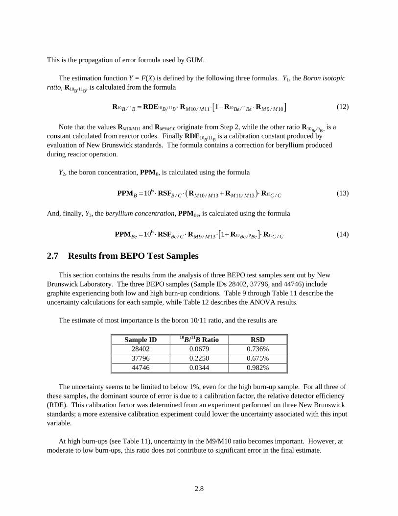
The estimation function Y = F(X) is defined by the following three formulas. Y1, the Boron isotopic

ratio, R10B/11B, is calculated from the formula

10 11 10 11 10 1110 11 9 101B/ B B/ B M / M Be/ Be M / M R RDE R R R (12)

Note that the values RM10/M11 and RM9/M10 originate from Step 2, while the other ratio R10Be/9Be is a

constant calculated from reactor codes. Finally RDE10B/11B is a calibration constant produced by

evaluation of New Brunswick standards. The formula contains a correction for beryllium produced

during reactor operation.

Y2, the boron concentration, PPMB, is calculated using the formula

136

10 13 11 1310B B / C M / M M / M C / C PPM RSF R R R (13)

And, finally, Y3, the beryllium concentration, PPMBe, is calculated using the formula

10 9 136

9 1310 1Be Be / C M / M Be / Be C / C PPM RSF R R R (14)

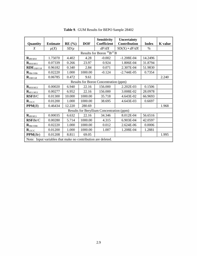
2.7 Results from BEPO Test Samples

This section contains the results from the analysis of three BEPO test samples sent out by New

Brunswick Laboratory. The three BEPO samples (Sample IDs 28402, 37796, and 44746) include

graphite experiencing both low and high burn-up conditions. Table 9 through Table 11 describe the

uncertainty calculations for each sample, while Table 12 describes the ANOVA results.

The estimate of most importance is the boron 10/11 ratio, and the results are

Sample ID 10

B/11

B Ratio RSD

28402 0.0679 0.736%

37796 0.2250 0.675%

44746 0.0344 0.982%

The uncertainty seems to be limited to below 1%, even for the high burn-up sample. For all three of

these samples, the dominant source of error is due to a calibration factor, the relative detector efficiency

(RDE). This calibration factor was determined from an experiment performed on three New Brunswick

standards; a more extensive calibration experiment could lower the uncertainty associated with this input

variable.

At high burn-ups (see Table 11), uncertainty in the M9/M10 ratio becomes important. However, at

moderate to low burn-ups, this ratio does not contribute to significant error in the final estimate.

2.9

Table 9. GUM Results for BEPO Sample 28402

Quantity Estimate RE (%) DOF

Sensitivity

Coefficient

Uncertainty

Contribution Index K value

X µ(X) SD/µ dF/dX SD(X) • dF/dX %

Results for Boron 10

B/11

B

RM9/M10 1.75070 4.402 4.28 -0.002 -1.208E-04 14.2496

RM10/M11 0.07339 0.266 23.97 0.924 1.806E-04 31.8794

RDE10B/11B 0.96182 0.340 2.84 0.071 2.307E-04 51.9830

R9Be/10Be 0.02220 1.000 1000.00 -0.124 -2.744E-05 0.7354

R10B/11B 0.06785 0.472 9.61 2.240

Results for Boron Concentration (ppm)

RM10/M13 0.00020 6.940 22.16 156.000 2.202E-03 0.1506

RM11/M13 0.00277 6.952 22.16 156.000 3.008E-02 28.0978

RSFB/C 0.01300 10.000 1000.00 35.718 4.643E-02 66.9693

R13C/C 0.01200 1.000 1000.00 38.695 4.643E-03 0.6697

PPM(B) 0.46434 12.220 280.69 1.968

Results for Beryllium Concentration (ppm)

RM9/M13 0.00035 6.632 22.16 34.346 8.012E-04 56.6516

RSFBe/C 0.00280 5.714 1000.00 4.315 6.903E-04 42.0597

R9Be/10Be 0.02220 1.000 1000.00 0.012 2.624E-06 0.0006

R13C/C 0.01200 1.000 1000.00 1.007 1.208E-04 1.2881

PPM(Be) 0.01208 8.811 69.05 1.995

Note: Input variables that make no contribution are deleted.

2.10



Sensitivity

Coefficient

Uncertainty




B/11

B

RM9/M10 0.01739 28.281 8.73 -0.005 -2.449E-05 0.0875

RM10/M11 0.23323 0.143 18.00 0.961 3.196E-04 14.8920

RDE10B/11B 0.96182 0.340 2.84 0.233 7.624E-04 84.7379

R9Be/10Be 0.02220 1.000 1000.00 -0.004 -8.660E-07 0.0001

R10B/11B 0.22424 0.369 3.94 2.793


RM10/M13 0.00084 17.054 7.37 156.000 2.226E-02 2.6250

RM11/M13 0.00359 17.189 7.29 156.000 9.632E-02 49.1316

RSFB/C 0.01300 10.000 1000.00 53.145 6.909E-02 25.2788

R13C/C 0.01200 1.000 1000.00 57.573 6.909E-03 0.2528

PPM(B) 0.69088 19.889 30.10 2.042


RM9/M13 0.00001 16.432 18.00 34.346 7.063E-05 88.9180

RSFBe/C 0.00280 5.714 1000.00 0.153 2.456E-05 10.7525

R9Be/10Be 0.02220 1.000 1000.00 0.000 9.334E-08 0.0002

R13C/C 0.01200 1.000 1000.00 0.036 4.298E-06 0.3293

PPM(Be) 0.00043 17.426 22.77 2.070


2.11



Sensitivity

Coefficient

Uncertainty




B/11

B

RM9/M10 4.43666 5.043 7.69 -0.001 -1.891E-04 47.0791

RM10/M11 0.03957 0.459 23.99 0.867 1.575E-04 32.6536

RDE10B/11B 0.96182 0.340 2.84 0.036 1.167E-04 17.9263

R9Be/10Be 0.02220 1.000 1000.00 -0.169 -3.749E-05 1.8512

R10B/11B 0.03431 0.803 22.44 2.071


RM10/M13 0.00009 11.825 10.44 156.000 1.726E-03 0.0854

RM11/M13 0.00237 11.629 11.14 156.000 4.297E-02 52.9439

RSFB/C 0.01300 10.000 1000.00 29.544 3.841E-02 42.3055

R13C/C 0.01200 1.000 1000.00 32.006 3.841E-03 0.4231

PPM(B) 0.38408 15.375 39.75 2.021


RM9/M13 0.00040 8.132 16.37 34.346 1.115E-03 66.2738

RSFBe/C 0.00280 5.714 1000.00 4.897 7.834E-04 32.7235

R9Be/10Be 0.02220 1.000 1000.00 0.013 2.978E-06 0.0005

R13C/C 0.01200 1.000 1000.00 1.143 1.371E-04 1.0022

PPM(Be) 0.01371 9.989 37.27 2.026


2.12

Table 12. ANOVA Results from BEPO Samples

Ratio

ANOVA Results %RE from Other Calc.

%RE %RE(Spot) %RE(Repl) Time-Series Poisson Cnt

Sample 28402

RM9/M10 1.750000 4.400 8.65e+00 3.62 0.285 0.1670

RM10/M11 0.073400 0.266 2.26e-01 1.08 0.196 0.1970

RM9/M13 0.000352 6.630 1.28e-05 28.90 0.476 0.1670

RM10/M13 0.000203 6.940 4.90e-10 30.30 0.504 0.1730

RM11/M13 0.002770 6.950 9.04e-06 30.30 0.490 0.0939

Sample 37796

RM9/M10 1.74e-02 28.300 5.46e+01 59.000 8.700 0.6610

RM10/M11 2.33e-01 0.143 9.01e-10 0.605 0.117 0.121

RM9/M13 1.25e-05 16.400 7.18e-06 69.700 8.320 0.6530

RM10/M13 8.37e-04 17.100 3.45e+01 29.900 1.270 0.1060

RM11/M13 3.59e-03 17.200 3.49e+01 29.700 1.260 0.0725

Sample 44746

RM9/M10 4.44e+00 5.040 11.600 9.45 0.416 0.242

RM10/M11 3.96e-02 0.459 0.738 1.89 0.250 0.234

RM9/M13 3.99e-04 8.130 15.100 28.40 0.908 0.271

RM10/M13 9.35e-05 11.800 25.100 31.70 1.010 0.237

RM11/M13 2.37e-03 11.600 24.200 32.80 1.060 0.116

The boron and beryllium concentrations seem to be consistent with what is known about the samples;

the boron concentration is approximately 0.5 ppm for all three samples. For the samples with the highest

burn-up (i.e., 28402 and 44746), the beryllium concentration is about 0.01 ppm, while the lowest burn-up

sample has a very much lower beryllium concentration (0.0004 ppm).

The ANOVA results presented in Table 12 merit a few comments. First note that the spot-to-spot

variability for the most important ratio RM10/M11 is near zero for all three samples. (It is, in fact, not

significantly different from zero.) Since spot-to-spot variability should include variability due to

contamination, this is an indication that the SIMS measurement protocol has successfully dealt with

contamination. Also note that RSD(repl) is approximately a factor of 5 greater that RSD (time-series), an

indication that the ANOVA analysis gives a much more realistic estimate of measurement uncertainty

than the standard deviation calculated from the time-series.

2.13

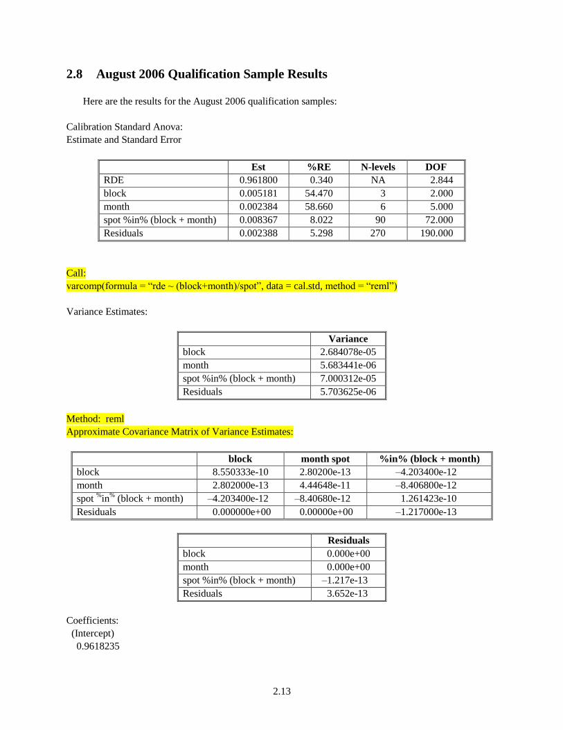
2.8 August 2006 Qualification Sample Results

Here are the results for the August 2006 qualification samples:

Calibration Standard Anova:

Estimate and Standard Error

Est %RE N-levels DOF

RDE 0.961800 0.340 NA 2.844

block 0.005181 54.470 3 2.000

month 0.002384 58.660 6 5.000

spot %in% (block + month) 0.008367 8.022 90 72.000

Residuals 0.002388 5.298 270 190.000

Call:

varcomp(formula = “rde ~ (block+month)/spot”, data = cal.std, method = “reml”)

Variance Estimates:

Variance

block 2.684078e-05

month 5.683441e-06

spot %in% (block + month) 7.000312e-05

Residuals 5.703625e-06

Method: reml

Approximate Covariance Matrix of Variance Estimates:

block month spot %in% (block + month)

block 8.550333e-10 2.80200e-13 –4.203400e-12

month 2.802000e-13 4.44648e-11 –8.406800e-12

spot %

in%

(block + month) –4.203400e-12 –8.40680e-12 1.261423e-10

Residuals 0.000000e+00 0.00000e+00 –1.217000e-13

Residuals

block 0.000e+00

month 0.000e+00

spot %in% (block + month) –1.217e-13

Residuals 3.652e-13

Coefficients:

(Intercept)

0.9618235

2.14

Approximate Covariance Matrix of Coefficients:

[1] 1.06931e-05

2.8.1 Results for Sample QA-21353 Anova Results

Replicate X Spot Design Matrix

1 2 3 4 5

1 3 3 3 3 3

2 3 3 3 3 3

3 3 3 3 3 3

MANOVA Estimates and Variance Components (in terms of percent relative error)

est RE.est RE.spot RE.rep RE.cycle RE.pois

M10.11 0.20000 0.233 0.142000 1.51 1.22e-01 0.11

Error Propagation and Estimates

Est RE dof Sensit Uncert Index

r.m10.m11 0.2000 0.233 49.60 0.96200 0.000449 56.6

rde.b10.b11 0.9620 0.340 2.84 0.20000 0.000654 82.4

Result 0.1920 0.412 6.08 NA NA NA

K-value: qt(.975,6.08)=2.44

2.8.2 Results for Sample QA-21361, ANOVA Results


1 2 3 4 5

1 3 3 3 3 3

2 3 3 3 3 3

3 3 3 3 3 3



M10.11 0.0789 0.242 3.40e-07 1.62 0.12 0.108



r.m10.m11 0.0789 0.242 45.00 0.96200 0.000183 57.9

rde.b10.b11 0.9620 0.340 2.84 0.07890 0.000258 81.5

Result 0.0759 0.417 6.34 NA NA NA

2.15

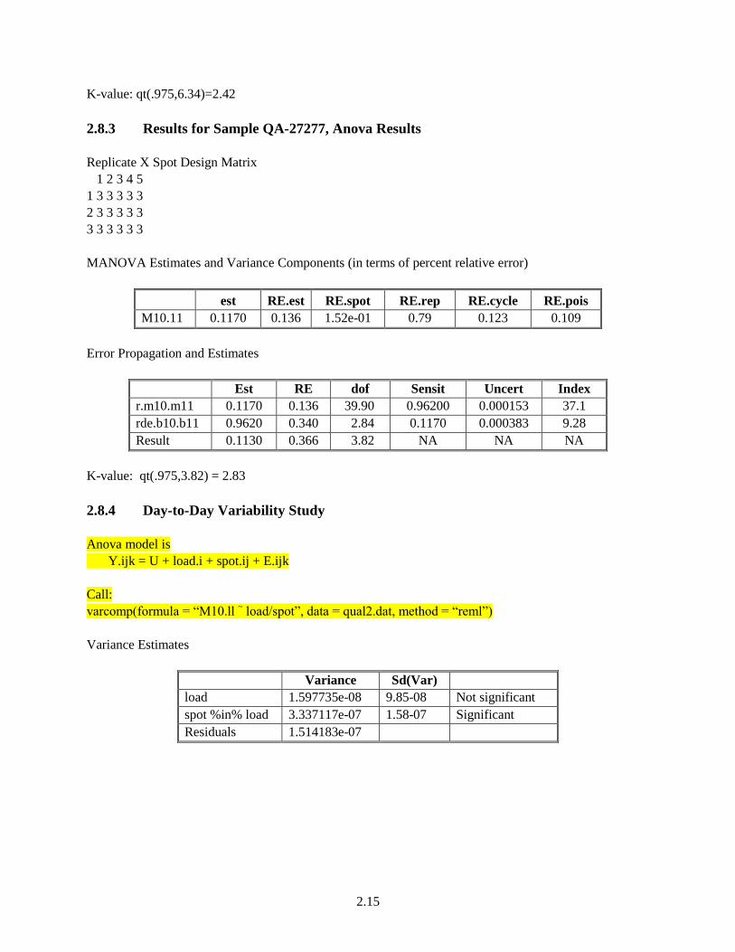
K-value: qt(.975,6.34)=2.42

2.8.3 Results for Sample QA-27277, Anova Results


1 2 3 4 5

1 3 3 3 3 3

2 3 3 3 3 3

3 3 3 3 3 3



M10.11 0.1170 0.136 1.52e-01 0.79 0.123 0.109



r.m10.m11 0.1170 0.136 39.90 0.96200 0.000153 37.1

rde.b10.b11 0.9620 0.340 2.84 0.1170 0.000383 9.28

Result 0.1130 0.366 3.82 NA NA NA

K-value: qt(.975,3.82) = 2.83

2.8.4 Day-to-Day Variability Study

Anova model is

Y.ijk = U + load.i + spot.ij + E.ijk

Call:

varcomp(formula = “M10.ll ~ load/spot”, data = qual2.dat, method = “reml”)

Variance Estimates

Variance Sd(Var)

load 1.597735e-08 9.85-08 Not significant

spot %in% load 3.337117e-07 1.58-07 Significant

Residuals 1.514183e-07

2.16

Method: reml

Approximate Covariance Matrix of Variance Estimates

load spot %in% load Residuals

load 9.69886e-15 –4.895350e-15 –2.09600e-17

spot %in% load –4.89535e-15 2.483763e-14 –7.25000e-16

Residuals –2.09600e-17 –7.250000e-16 2.28818e-15

Coefficients:

(Intercept)

0.1986207

Approximate Covariance Matrix of Coefficients:

[1] 3.104391e-08

2.8.5 GUM Tables for Qualification samples

Since the qualification samples were not irradiated, the samples were not expected to contain 9Be and

10Be. Thus, Be isotopes and

13C were not included in analyses, as for the NBL BEPO samples, and the

GUM uncertainty budget for the NBL QA samples below is simpler.

Table 13. GUM Table for Qualification Sample 21353 SIMS Results


Sensitivity

Coefficient

Uncertainty



RM9/M10 n.d n.d n.d

RM10/M11 0.20009 0.233 49.61 0.962 4.492E-04 32.0339

RDE10B/11B 0.96182 0.340 2.84 0.200 6.543E-04 67.9661

R10B/11B 0.19245 0.412 6.08 2.439


2.17



Sensitivity

Coefficient

Uncertainty



RM9/M10 n.d n.d n.d

RM10/M11 0.07889 0.242 45.00 0.962 1.833E-04 33.5498

RDE10B/11B 0.96182 0.340 2.84 0.079 2.580E-04 66.4502

R10B/11B 0.07588 0.417 6.34 2.416




Sensitivity

Coefficient

Uncertainty



RM9/M10 n.d n.d n.d

RM10/M11 0.11701 0.136 39.95 0.962 1.530E-04 13.7915

RDE10B/11B 0.96182 0.340 2.84 0.117 3.826E-04 86.2085

R10B/11B 0.11254 0.366 3.82 2.829


3.1

3.0 TIMS Measurements

3.1 Samples for TIMS Analyses, Preparation and Processing

In Fall 2005, one set of three samples from New Brunswick Laboratory (NBL) were addressed to

Steve Petersen for TIMS analysis, and included BEPO samples numbered 10431, 16819, and 27727, and

three blanks numbered B-17, B-27, and B-58. A second set of three samples from NBL was addressed to

David Gerlach for SIMS analysis, and these included BEPO samples 28402, 37796, and 44746, and three

blanks numbered B-49, B-64, and B-77. All cores were trimmed by tooling, and lightly cleaned by CO2

pellet blasting. Small discs were cut from the second set of samples for SIMS analysis, with the

remainder of each used for TIMS preparation.

The GIRM Phase II QA samples were received from NBL in May 2006, and consisted of UCAR

graphite plugs doped with solutions containing uranium and plutonium. The three samples received at

PNNL for TIMS analysis were numbered UCAR 25-B, UCAR 41-B, and UCAR 57-B. These were not

trimmed or prepared in the manner above, but the as-received samples were ashed, as in step 1 below.

The general sample preparation procedure for TIMS analysis includes the following steps:

1. Samples ashed and ash acid digested, ending up in HCl.

2. 10% of ash solution taken for unspiked U separation and TIMS analysis; 233U/238U ratios

determined by TIMS analysis rather than ICPMS analyses as used earlier.

3. Remaining 90% spiked with mixed U-233 + Pu-244 spike; Pu-244 spike amount chosen to be

appropriate for sample based on unspiked U isotope ratios, to minimize spike correction on minor Pu

isotopes, and because Pu contents were expected to vary by up to 300-fold.

4. Portion of separated spiked U fraction aliquotted for Pu TIMS analysis and additional U TIMS

analysis based on observed U total contents, 2 ng U usual amount preferred, 1 to 3 pg Pu preferred

(more for low burnup samples).

5. Total U contents calculated based on sample and aliquot weights, and spiked and unspiked

233U/238U ratios, since many samples contain U-233 already. Total Pu contents determined based

on measured amount of Pu-244 added.

The six NBL BEPO samples were prepared following these steps, resulting in both spiked and

unspiked U fractions analyzed by TIMS. Based on instructions from NBL, the three QA samples were

not split following our usual procedure as outline above, and instead, the entire sample was processed and

combined with the U and Pu spikes.

Uranium samples for TIMS analysis are prepared by solution loading onto carburized Re filaments.

Plutonium fractions are equilibrated with single anion resin beads that are loaded onto carburized Re

filaments to make a better point source for thermal ion emission.

3.2

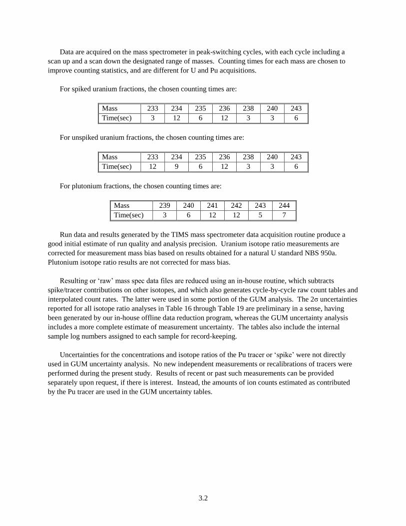
Data are acquired on the mass spectrometer in peak-switching cycles, with each cycle including a

scan up and a scan down the designated range of masses. Counting times for each mass are chosen to

improve counting statistics, and are different for U and Pu acquisitions.

For spiked uranium fractions, the chosen counting times are:

Mass 233 234 235 236 238 240 243

Time(sec) 3 12 6 12 3 3 6

For unspiked uranium fractions, the chosen counting times are:

Mass 233 234 235 236 238 240 243

Time(sec) 12 9 6 12 3 3 6

For plutonium fractions, the chosen counting times are:

Mass 239 240 241 242 243 244

Time(sec) 3 6 12 12 5 7

Run data and results generated by the TIMS mass spectrometer data acquisition routine produce a

good initial estimate of run quality and analysis precision. Uranium isotope ratio measurements are

corrected for measurement mass bias based on results obtained for a natural U standard NBS 950a.

Plutonium isotope ratio results are not corrected for mass bias.

Resulting or ‘raw’ mass spec data files are reduced using an in-house routine, which subtracts

spike/tracer contributions on other isotopes, and which also generates cycle-by-cycle raw count tables and

interpolated count rates. The latter were used in some portion of the GUM analysis. The 2σ uncertainties

reported for all isotope ratio analyses in Table 16 through Table 19 are preliminary in a sense, having

been generated by our in-house offline data reduction program, whereas the GUM uncertainty analysis

includes a more complete estimate of measurement uncertainty. The tables also include the internal

sample log numbers assigned to each sample for record-keeping.

Uncertainties for the concentrations and isotope ratios of the Pu tracer or ‘spike’ were not directly

used in GUM uncertainty analysis. No new independent measurements or recalibrations of tracers were

performed during the present study. Results of recent or past such measurements can be provided

separately upon request, if there is interest. Instead, the amounts of ion counts estimated as contributed

by the Pu tracer are used in the GUM uncertainty tables.

3.3

Table 16. Uranium TIMS Results for NBL BEPO Samples

NBL

BEPO

Sample

PNNL

Sample

Log # U 233/238* 33/38 2sig U 234/238 34/38 2 sig U235/238 35/38 2sig U236/238 36/38 2sig

Total U,

ng/g

16819 U83599 2.251E-03 1.156E-05 6.126E-05 1.160E-05 7.243E-03 1.928E-05 7.150E-06 4.000E-07 2.34

10431 U83600 1.377E-02 3.310E-05 2.459E-04 2.180E-06 4.919E-03 1.728E-05 3.742E-04 2.680E-06 1.58

27727 U83601 4.970E-03 2.412E-05 7.156E-05 1.180E-05 6.649E-03 2.420E-05 8.439E-05 1.280E-06 11.75

28402 U28402 8.025E-03 2.838E-05 1.229E-04 1.480E-06 5.839E-03 1.472E-05 2.347E-04 2.060E-06 20.38

37796 U37796 9.105E-04 7.460E-06 6.071E-05 1.180E-06 7.057E-03 2.170E-05 2.823E-05 9.800E-07 62.59

44746 U44746 1.418E-02 6.610E-05 2.774E-04 3.100E-06 5.450E-03 2.936E-05 3.045E-04 3.440E-06 0.37

*233U/238U ratios measured in sample aliquots without added 233U spike/tracer

Table 17. Plutonium TIMS Results for NBL BEPO Samples

NBL BEPO

Sample

PNNL

Sample Log # Pu 240/239 40/39 2sig Pu 241/239 41/39 2sig Pu 242/239 42/39 2sig

Total Pu,

pg/g

16819 P83599 7.924E-03 8.200E-05 8.450E-05 7.400E-06 5.870E-05 6.600E-06 0.47

10431 P83600 1.303E-01 3.042E-04 2.645E-03 3.318E-05 1.152E-03 2.172E-05 82.81

27727 P83601 2.176E-02 5.266E-05 4.907E-05 1.820E-06 8.000E-06 3.160E-06 6.07

28402 P83673 7.424E-02 2.335E-04 8.734E-04 4.240E-05 2.154E-04 7.540E-06 50.62

37796 P83749 8.973E-03 1.520E-04 3.600E-05 2.000E-05 3.110E-05 1.660E-05 0.77

44746 P83674.1 1.153E-01 1.700E-04 2.082E-03 2.000E-05 8.084E-04 8.800E-06 12.28

P83674.2 1.150E-01 1.250E-04 2.068E-03 1.360E-05 8.121E-04 5.000E-06

3.4

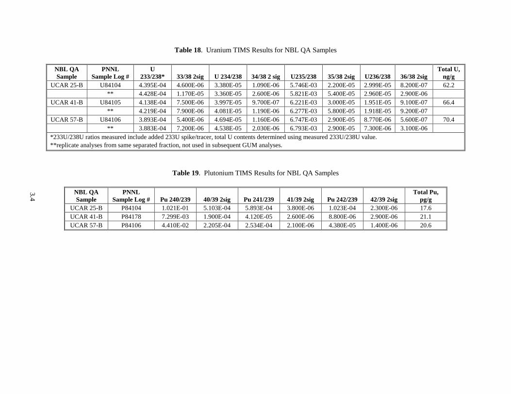
Table 18. Uranium TIMS Results for NBL QA Samples

NBL QA

Sample

PNNL

Sample Log #

U

233/238* 33/38 2sig U 234/238 34/38 2 sig U235/238 35/38 2sig U236/238 36/38 2sig

Total U,

ng/g

UCAR 25-B U84104 4.395E-04 4.600E-06 3.380E-05 1.090E-06 5.746E-03 2.200E-05 2.999E-05 8.200E-07 62.2

** 4.428E-04 1.170E-05 3.360E-05 2.600E-06 5.821E-03 5.400E-05 2.960E-05 2.900E-06

UCAR 41-B U84105 4.138E-04 7.500E-06 3.997E-05 9.700E-07 6.221E-03 3.000E-05 1.951E-05 9.100E-07 66.4

** 4.219E-04 7.900E-06 4.081E-05 1.190E-06 6.277E-03 5.800E-05 1.918E-05 9.200E-07

UCAR 57-B U84106 3.893E-04 5.400E-06 4.694E-05 1.160E-06 6.747E-03 2.900E-05 8.770E-06 5.600E-07 70.4

** 3.883E-04 7.200E-06 4.538E-05 2.030E-06 6.793E-03 2.900E-05 7.300E-06 3.100E-06

*233U/238U ratios measured include added 233U spike/tracer, total U contents determined using measured 233U/238U value.

**replicate analyses from same separated fraction, not used in subsequent GUM analyses.

Table 19. Plutonium TIMS Results for NBL QA Samples

NBL QA

Sample

PNNL

Sample Log # Pu 240/239 40/39 2sig Pu 241/239 41/39 2sig Pu 242/239 42/39 2sig

Total Pu,

pg/g

UCAR 25-B P84104 1.021E-01 5.103E-04 5.893E-04 3.800E-06 1.023E-04 2.300E-06 17.6

UCAR 41-B P84178 7.299E-03 1.900E-04 4.120E-05 2.600E-06 8.800E-06 2.900E-06 21.1

UCAR 57-B P84106 4.410E-02 2.205E-04 2.534E-04 2.100E-06 4.380E-05 1.400E-06 20.6

3.5

The contents of U and Pu determined by adding spikes or tracers as outlined above are calculated

separately in a spreadsheet which includes initial (unprocessed) sample weights, weights of the spiked

and unspiked aliquots (for uranium), and measured isotope ratios corrected for spike/tracer contributions

on all isotopes. The U and Pu contents determined in the qualification samples compared very favorably

with the amounts estimated that were added, as stated in the shipping memo for the samples. The U and

Pu contents in the 6 BEPO cores sent from NBL vary a bit, but we have seen a similar range of variation

in samples taken from the 19 BEPO cores studied at PNNL, and in some cases, even in intra-block

variability over relatively small areas.

As outlined in subsequent sections, GUM analyses of Pu results included uncertainty due to

subtraction of minor amounts of isotope present in the spike or tracer added. Results of U TIMS analyses

on unspiked aliquots were used for GUM analysis of U data for the six NBL BEPO cores. Since the three

NBL QA core solutions prepared were not split before adding U spike, the GUM analyses for these three

samples were performed without correction of minor isotopes present in the U spike, at this time.

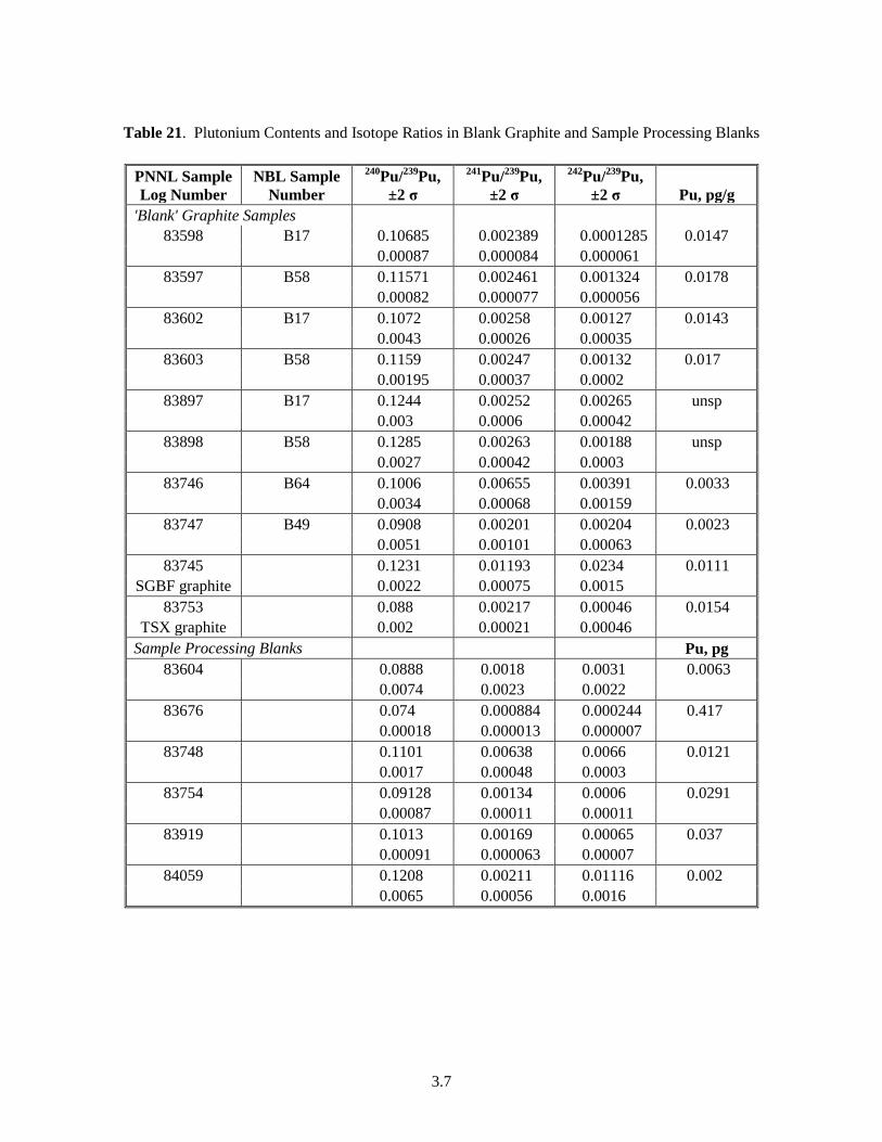
3.2 TIMS Blanks

In the current study, two types of ‘blanks’ were prepared and analyzed. Uranium and plutonium

tracers were added to each to precisely determine U and Pu contents. One type consisted of high-purity

UCAR graphite powder, pressed into plugs, provided by New Brunswick Laboratory. Two additional

samples of very high-purity graphite from PNNL archives were also processed for blank Pu contents for

comparison. These graphite ‘blanks’ were ashed and dissolved as in other types of samples, and the

tracers usually added to 80% of the sample digestion. For two of the graphite blanks, B17 and B58,

tracers were added to 10% of the sample solution for an initial determination, and tracers were later added

to 80% of the sample solution for a replicate determination. The NBL blank graphite samples ranged in

U contents from 0.4 to 2 ng/g, and were also found to contain small amounts of Pu (Table 20 and

Table 21). The Pu contents in the blank graphite samples ranged from 3 fg to 18 fg, and were similar in

amounts to sample processing blanks.

The other type of TIMS blank includes sample processing blanks where an empty quartz glass boat is

heated in the furnace, washed with acid as for an ash removal step and U and Pu tracers added to the

solution, followed by the same U and Pu separation procedures. Sample processing blanks are usually

prepared along with samples, and the various blanks in Table 20 and Table 21 accompanied sets of NBL

BEPO or qualification samples. Blank levels of U ranged from <1 pg to 42 pg (Table 20) and most

resembled natural U or were slightly enriched in 235

U. Sample processing blanks for Pu ranged from 2 to

37 fg, except for one catastrophic blank of 417 fg, which was clearly a case of cross contamination from

the sample adjacent during processing, due to similarities in the Pu isotope ratios.

3.6

Table 20. Uranium Contents and Isotope Ratios in Blank Graphite and Sample Processing Blanks

PNNL Sample

Log Number

NBL Sample

Number 234

U/238

U, ±2 σ 235

U/238

U, ±2 σ U, ng/g

'Blank' Graphite Samples

83596 B17 0.000043 0.00757 1.14

0.000038 0.00069

83597 B58 0.0000519 0.007145 0.934

0.0000118 0.000164

83602 B17 0.0000564 0.007125 1.12

0.0000016 0.000034

83603 B58 0.0000614 0.007291 0.939

0.000096 0.000032

83746 B64 0.000056 0.007257 2.02

0.0000024 0.000034

83747 B49 0.00005415 0.007327 0.421

0.0000017 0.000032

Sample Processing Blanks Total ng

83598 0.000032 0.00608 0.0125

0.000042 0.00025

83615 0.000115 0.006848 0.0037

0.0000064 0.000098

83676 0.0001038 0.006401 0.0317

0.0000025 0.00003

83748 0.0000635 0.007397 0.0203

0.0000032 0.000042

83819 0.000158 0.00794 0.0423

0.0000067 0.000054

83825 0.0001415 0.007585 0.0187

0.0000109 0.000086

84059 0.0000857 0.008448 0.019

0.0000041 0.000072

84107 0.000117 0.00753 0.0038

0.000048 0.00031

84203 0.00024 0.0237 0.0008

0.00032 0.0117

3.7

Table 21. Plutonium Contents and Isotope Ratios in Blank Graphite and Sample Processing Blanks

PNNL Sample

Log Number

NBL Sample

Number

240Pu/

239Pu,

±2 σ

241Pu/

239Pu,

±2 σ

242Pu/

239Pu,

±2 σ Pu, pg/g

'Blank' Graphite Samples

83598 B17 0.10685 0.002389 0.0001285 0.0147

0.00087 0.000084 0.000061

83597 B58 0.11571 0.002461 0.001324 0.0178

0.00082 0.000077 0.000056

83602 B17 0.1072 0.00258 0.00127 0.0143

0.0043 0.00026 0.00035

83603 B58 0.1159 0.00247 0.00132 0.017

0.00195 0.00037 0.0002

83897 B17 0.1244 0.00252 0.00265 unsp

0.003 0.0006 0.00042

83898 B58 0.1285 0.00263 0.00188 unsp

0.0027 0.00042 0.0003

83746 B64 0.1006 0.00655 0.00391 0.0033

0.0034 0.00068 0.00159

83747 B49 0.0908 0.00201 0.00204 0.0023

0.0051 0.00101 0.00063

83745 0.1231 0.01193 0.0234 0.0111

SGBF graphite 0.0022 0.00075 0.0015

83753 0.088 0.00217 0.00046 0.0154

TSX graphite 0.002 0.00021 0.00046

Sample Processing Blanks Pu, pg

83604 0.0888 0.0018 0.0031 0.0063

0.0074 0.0023 0.0022

83676 0.074 0.000884 0.000244 0.417

0.00018 0.000013 0.000007

83748 0.1101 0.00638 0.0066 0.0121

0.0017 0.00048 0.0003

83754 0.09128 0.00134 0.0006 0.0291

0.00087 0.00011 0.00011

83919 0.1013 0.00169 0.00065 0.037

0.00091 0.000063 0.00007

84059 0.1208 0.00211 0.01116 0.002

0.0065 0.00056 0.0016

3.8

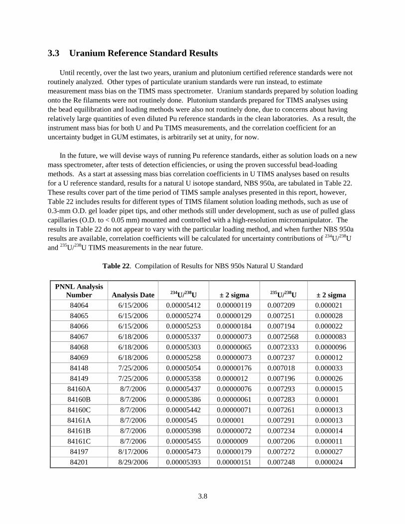
3.3 Uranium Reference Standard Results

Until recently, over the last two years, uranium and plutonium certified reference standards were not

routinely analyzed. Other types of particulate uranium standards were run instead, to estimate

measurement mass bias on the TIMS mass spectrometer. Uranium standards prepared by solution loading

onto the Re filaments were not routinely done. Plutonium standards prepared for TIMS analyses using

the bead equilibration and loading methods were also not routinely done, due to concerns about having

relatively large quantities of even diluted Pu reference standards in the clean laboratories. As a result, the

instrument mass bias for both U and Pu TIMS measurements, and the correlation coefficient for an

uncertainty budget in GUM estimates, is arbitrarily set at unity, for now.

In the future, we will devise ways of running Pu reference standards, either as solution loads on a new

mass spectrometer, after tests of detection efficiencies, or using the proven successful bead-loading

methods. As a start at assessing mass bias correlation coefficients in U TIMS analyses based on results

for a U reference standard, results for a natural U isotope standard, NBS 950a, are tabulated in Table 22.

These results cover part of the time period of TIMS sample analyses presented in this report, however,

Table 22 includes results for different types of TIMS filament solution loading methods, such as use of

0.3-mm O.D. gel loader pipet tips, and other methods still under development, such as use of pulled glass

capillaries (O.D. to < 0.05 mm) mounted and controlled with a high-resolution micromanipulator. The

results in Table 22 do not appear to vary with the particular loading method, and when further NBS 950a

results are available, correlation coefficients will be calculated for uncertainty contributions of 234

U/238

U

and 235

U/238

U TIMS measurements in the near future.

Table 22. Compilation of Results for NBS 950s Natural U Standard

PNNL Analysis

Number Analysis Date 234

U/238

U ± 2 sigma 235

U/238

U ± 2 sigma

84064 6/15/2006 0.00005412 0.00000119 0.007209 0.000021

84065 6/15/2006 0.00005274 0.00000129 0.007251 0.000028

84066 6/15/2006 0.00005253 0.00000184 0.007194 0.000022

84067 6/18/2006 0.00005337 0.00000073 0.0072568 0.0000083

84068 6/18/2006 0.00005303 0.00000065 0.0072333 0.0000096

84069 6/18/2006 0.00005258 0.00000073 0.007237 0.000012

84148 7/25/2006 0.00005054 0.00000176 0.007018 0.000033

84149 7/25/2006 0.00005358 0.0000012 0.007196 0.000026

84160A 8/7/2006 0.00005437 0.00000076 0.007293 0.000015

84160B 8/7/2006 0.00005386 0.00000061 0.007283 0.00001

84160C 8/7/2006 0.00005442 0.00000071 0.007261 0.000013

84161A 8/7/2006 0.0000545 0.000001 0.007291 0.000013

84161B 8/7/2006 0.00005398 0.00000072 0.007234 0.000014

84161C 8/7/2006 0.00005455 0.0000009 0.007206 0.000011

84197 8/17/2006 0.00005473 0.00000179 0.007272 0.000027

84201 8/29/2006 0.00005393 0.00000151 0.007248 0.000024

3.9

PNNL Analysis

Number Analysis Date 234

U/238

U ± 2 sigma 235

U/238

U ± 2 sigma

84202 8/29/2006 0.00005505 0.00000157 0.007275 0.000021

84425A 10/20/2006 0.00005477 0.00000184 0.007277 0.000024

84425B 10/20/2006 0.00005299 0.00000126 0.0072473 0.0000191

84425C 10/27/2006 0.00005525 0.00000125 0.0072654 0.0000187

84550A 1/4/2007 0.0000549 0.0000021 0.007256 0.00005

84550B 1/4/2007 0.00005414 0.00000166 0.007241 0.000021

84597 2/9/2007 0.00005574 0.00000142 0.007286 0.000028

84599 2/9/2007 0.00005587 0.00000157 0.007259 0.000056

84600 2/9/2007 0.00005413 0.00000192 0.007241 0.000035

84601 2/9/2007 0.00005441 0.00000168 0.007243 0.000028

84602 2/9/2007 0.00005596 0.00000162 0.007272 0.000023

84615 2/23/2007 0.00005363 0.00000189 0.007222 0.000055

84616 2/23/2007 0.0000523 0.0000021 0.007134 0.000034

84617 2/23/2007 0.00005433 0.00000148 0.007237 0.000047

84618 2/23/2007 0.0000561 0.0000034 0.007342 0.000043

84619 2/23/2007 0.00005461 0.0000019 0.00732 0.000024

84620 2/23/2007 0.0000546 0.0000023 0.0073356 0.000025

84621 2/26/2007 0.0000551 0.0000016 0.007245 0.000034

84622 2/26/2007 0.00005376 0.00000159 0.007202 0.000024

84623 2/26/2007 0.0000541 0.0000026 0.007265 0.000046

84624 2/26/2007 0.00005551 0.0000015 0.007245 0.000018

84625 2/26/2007 0.0000544 0.000002 0.007223 0.000049

84626 2/26/2007 0.00005436 0.00000141 0.007212 0.000033

84670 3/16/2006 0.00005371 0.00000193 0.007212 0.000026

84671 3/16/2006 0.000054 0.00000158 0.007235 0.000022

84672 3/16/2006 0.00005322 0.00000132 0.007248 0.000023

Mean ratio or 41 measurements 5.41374E-05 0.007243414

Sample standard deviation 1.08619E-06 5.24712E-05

Sample RSD 2.01% 0.72%

Average measurement uncertainty 2.81% 0.37%

3.4 TIMS Estimation Procedure

For purposes of description, we have organized the estimation procedure into four steps. These steps

are performed by an in-hour data reduction software package using raw data files from the mass

spectrometer. Table 20 through Table 22 present TIMS results with 2-sigma uncertainties calculated by

the program, although these will be slightly lower than GUM uncertainty estimates as shown later.

3.10

Step 1: Calculate corrected count rates.

Step 2: Calculate atomic ratios for each acquisition.

Step 3: Calculate mean atomic ratios (i.e., final estimates).

Step 4: Calculate corrected ratios.

3.4.1 Step 1: Calculate Corrected Count Rates

The gross counts, cx,i, are corrected for dead time, interpolated, and corrected for background, to

produce a corrected count rate, rx,i. The index x identifies the AMU being measured, while i identifies the

acquisition time (i.e., duty cycle) that the count is associated with. The formula describing these

operations is:

x,ix,i tot ,x,i

x x,i

cr b

t c

(15)

where

τ = is the instrument dead time

tx = acquisition counting time for mass x

btot,x,i = Total background count rate. This is composed of three components that

are due to the detector, mass spectral, and tracer impurity.

tot,x,i det mspec,x,i tracer,x,ib =b +b +b (16)

bdet = Detector dark noise, the same for each mass and acquisition

bmspec,x,i = fx.tracer(rtracer,i - bdet) = This is correction for M243 (r243 uncorrected for background)

btracer,x,i = Fx.tracer • rtracer,i = This is correction for impurities in the tracer. Fx.tracer estimated from

analysis of tracer.

fx.tracer = Mass spec correction factor to AMU x for tracer 243

Fx.tracer = Impurity corection factor for tracer.

3.4.2 Step 2: Calculate Atomic Ratios

x,i

xy,iy ,i

rR

r (17)

3.11

3.4.3 Step 3: Calculate Means

The estimate for isotopic ratio x/y is calculated by

1

1N

xy i xy,i

i

R W RW

(18)

with the weights Wi = 1/se(Rxy,i)2, and W+ = ΣWi.

The standard error can be calculated with either of two formulas; first, via propagation of error

(POE):

2 1

xyse R W (19)

or, empirically, from the replicate measurements, Rxy,i:

2 2

1

1N

ixy xy,i xy

i

Wse R R R

N W

(20)

It should be noted that either calculation of standard error does not include systematic background

correction errors, such as those produced by bdet, for example.

3.4.4 Step 4: Correct Means for Bias

xy. final xy xyR CF R (21)

where CFxy is the correction due to mass and instrument bias. CFxy should be determined from a

calibration experiment using NBL standards, but this experiment hasn’t been run. We assume:

CFxy = 1

RE(CFxy) = 0.5%

3.5 GUM Version of Estimation Procedure for TIMS data

The systematic effects of background correction are dealt with using the approximation

2

1 1 1 x.ixy tot xy tot.x tot.x.i tot .y

y.i y.xi i

rR b R b b b

N r N r (22)

Uncertainty Calculation Details:

3.12

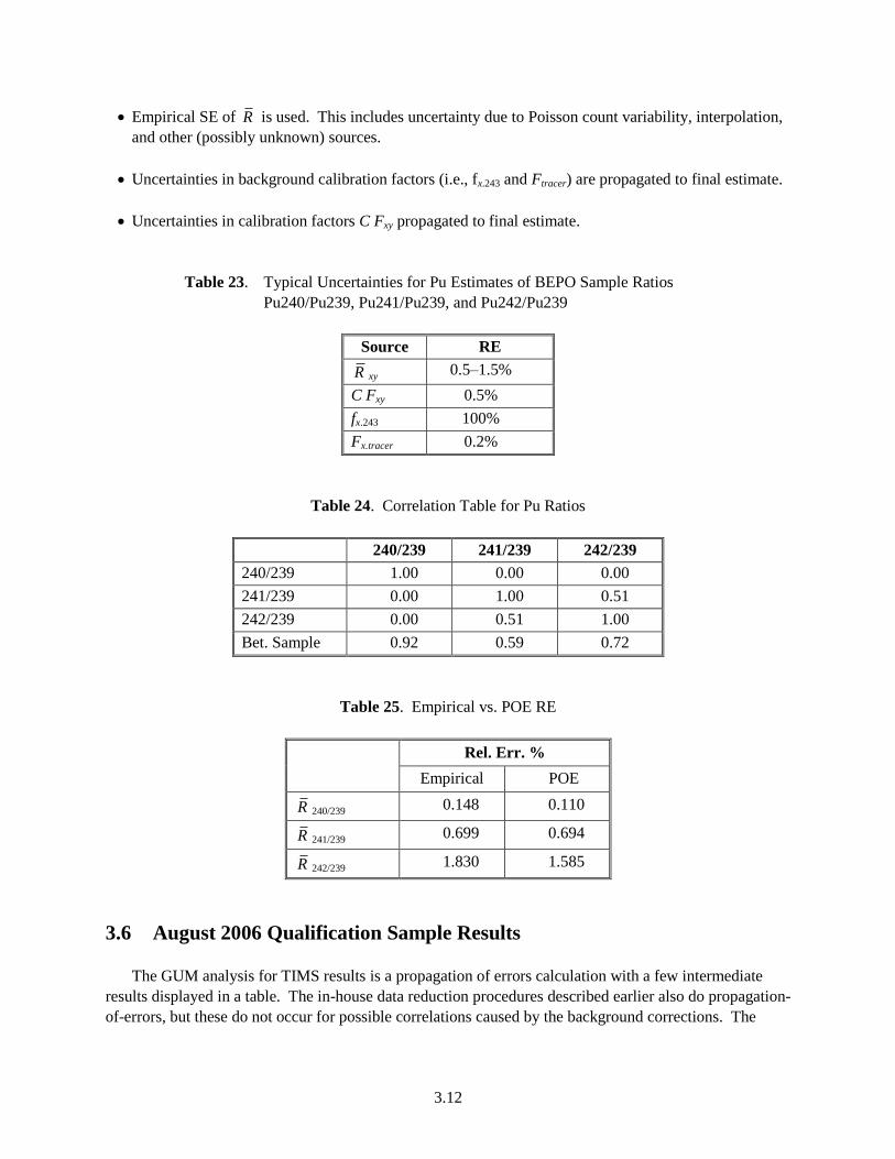
Empirical SE of R is used. This includes uncertainty due to Poisson count variability, interpolation,

and other (possibly unknown) sources.

Uncertainties in background calibration factors (i.e., fx.243 and Ftracer) are propagated to final estimate.

Uncertainties in calibration factors C Fxy propagated to final estimate.

Table 23. Typical Uncertainties for Pu Estimates of BEPO Sample Ratios

Pu240/Pu239, Pu241/Pu239, and Pu242/Pu239

Source RE

R xy 0.5–1.5%

C Fxy 0.5%

fx.243 100%

Fx.tracer 0.2%

Table 24. Correlation Table for Pu Ratios

240/239 241/239 242/239

240/239 1.00 0.00 0.00

241/239 0.00 1.00 0.51

242/239 0.00 0.51 1.00

Bet. Sample 0.92 0.59 0.72

Table 25. Empirical vs. POE RE

Rel. Err. %

Empirical POE

R 240/239 0.148 0.110

R 241/239 0.699 0.694

R 242/239 1.830 1.585

3.6 August 2006 Qualification Sample Results

The GUM analysis for TIMS results is a propagation of errors calculation with a few intermediate

results displayed in a table. The in-house data reduction procedures described earlier also do propagation-

of-errors, but these do not occur for possible correlations caused by the background corrections. The

3.13

GUM approach here then is really as an added-on component performing an additional correction to the

in-house data reduction results.

As an example of this, let us consider Sample 84104. Required inputs to the calculation include

calibration parameters used in TIMS estimation, and corrected count-rates and associated uncertainties.

The calibration parameter table lists the calibration parameter (as “est”), its uncertainty (sd), and its

degrees of freedom (dof). The calibration parameter table for Sample 84104 is shown in Table 26:

In Table 26, the parameter names identify quantities appearing in the basic in-house data reduction

estimation formulas as outlined earlier, to be used in subsequent GUM tables. For example,

b.det = background correction for dark detector noise

b.mspec = background correction counted at mass 243

b.tracer, 239 = background contributed by small amounts in added tracer

The only significant difference between quantities in Table 26 and those appearing in Steve’s

formulas is that some GUM table quantities represent averages. For example, b.mspec above is the

average of Steve’s b.mspec.i values (with i representing accumulation time). Other required inputs

inlcude corrected count rates (and associated POE standard deviation) for each atomic mass unit used in

the calculation. Here is an example for Sample 84104:

Table 26. Calibration Parameter Table for Sample 84104

Parameter Est. sd dof

b.det 0.156667 0.016744 28

b.mspec 0.4113 0 Inf

f.243 1 1 Inf

b.tracer.239 2.82E-01 0 Inf

b.tracer.240 5.64E+00 0 Inf

b.tracer.241 7.64E-01 0 Inf

b.tracer.242 1.11E+01 0 Inf

F.tracer.239 3.45E-04 1.00E-06 100

F.tracer.240 6.90E-03 5.00E-05 100

F.tracer.241 9.35E-04 2.00E-06 100

F.tracer.242 1.36E-02 3.00E-05 100

CF.xy 1 0.005 Inf

3.14

Table 27. Example of Corrected Count-Rate Table for Sample 84104, Based on Interpolated Count

Rates Supplied by PNNL TIMS Data Reduction Program

amu.239 sd.239 amu.240 sd.240 amu.241 sd.241 amu.242 sd.242

471200.80 588.23 48930.62 128.02 279.64 7.07 45.29 3.91

409165.35 534.26 41842.03 118.35 250.92 7.14 43.31 5.01

393071.95 518.75 39915.86 115.57 220.14 6.17 30.29 2.96

. . . . . . . .

. . . . . . . .

. . . . . . . .

6767.12 63.05 685.69 15.12 3.79 0.81 1.04 0.55

5768.89 58.77 594.56 14.08 3.15 0.74 0.27 0.33

2035.04 34.30 207.14 8.33 0.25 0.58 –0.15 0.55

The values in this table are supposed to represent the corrected count rates as calculated by the in-

house data reduction described earlier, as represented by the notation, r.x.i and se(r.x.i); the count rate for

amu “x” at acquisition time “i”.

The Gum table that is calculated from this input data should contain all the calibration factors present

in the above table. However, to simplify the table, we instead use an intermediate result into the GUM

table, b.tot, which is defined by

b.tot.x = b.det + b.mspec + b.tracer.x

Below is an intermediate GUM table provided as an example that describes the relationship between

b.tot.239 and the above inputs.

Table 28. GUM Relationship between Total Ion Counts for Mass 239 and Preceding Data Inputs

(Table 26 and Table 27).


b.det 1.57e-01 10.700 2.80e+01 0.00e+00 0.000000 0.000

b.mspec 5.68e-01 0.000 Inf 1.00e+00 0.000000 0.000

f.243 1.00e+00 100.000 Inf 4.11e-01 0.411000 100.000

b.tracer.239 8.17e+02 0.000 Inf 3.45e-04 0.000000 0.000

b.tracer.240 8.17e+02 0.000 Inf 0.00e+00 0.000000 0.000

b.tracer.241 8.17e+02 0.000 Inf 0.00e+00 0.000000 0.000

b.tracer.242 8.16e+02 0.000 Inf 0.00e+00 0.000000 0.000

F.tracer.239 3.45e-04 0.290 1.00e+02 8.17e+02 0.000817 0.199

F.tracer.240 6.90e-03 0.725 1.00e+02 0.00e+00 0.000000 0.000

F.tracer.241 9.35e-04 0.214 1.00e+02 0.00e+00 0.000000 0.000

F.tracer.242 1.36e-02 0.221 1.00e+02 0.00e+00 0.000000 0.000

Result 8.50e-01 48.400 6.41e+12 NA NA NA

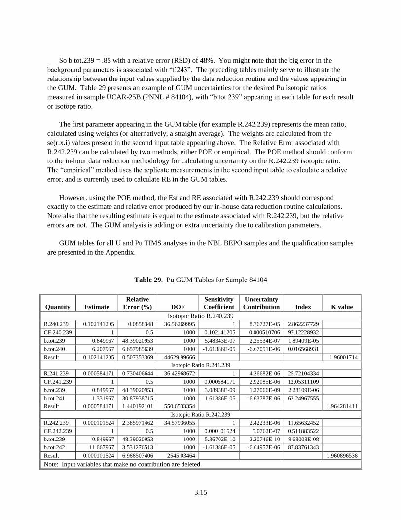
3.15

So b.tot.239 = .85 with a relative error (RSD) of 48%. You might note that the big error in the

background parameters is associated with “f.243”. The preceding tables mainly serve to illustrate the

relationship between the input values supplied by the data reduction routine and the values appearing in

the GUM. Table 29 presents an example of GUM uncertainties for the desired Pu isotopic ratios

measured in sample UCAR-25B (PNNL # 84104), with “b.tot.239” appearing in each table for each result

or isotope ratio.

The first parameter appearing in the GUM table (for example R.242.239) represents the mean ratio,

calculated using weights (or alternatively, a straight average). The weights are calculated from the

se(r.x.i) values present in the second input table appearing above. The Relative Error associated with

R.242.239 can be calculated by two methods, either POE or empirical. The POE method should conform

to the in-hour data reduction methodology for calculating uncertainty on the R.242.239 isotopic ratio.

The “empirical” method uses the replicate measurements in the second input table to calculate a relative

error, and is currently used to calculate RE in the GUM tables.

However, using the POE method, the Est and RE associated with R.242.239 should correspond

exactly to the estimate and relative error produced by our in-house data reduction routine calculations.

Note also that the resulting estimate is equal to the estimate associated with R.242.239, but the relative

errors are not. The GUM analysis is adding on extra uncertainty due to calibration parameters.

GUM tables for all U and Pu TIMS analyses in the NBL BEPO samples and the qualification samples

are presented in the Appendix.

Table 29. Pu GUM Tables for Sample 84104

Quantity Estimate

Relative

Error (%) DOF

Sensitivity

Coefficient

Uncertainty


Isotopic Ratio R.240.239

R.240.239 0.102141205 0.0858348 36.56269995 1 8.76727E-05 2.862237729

CF.240.239 1 0.5 1000 0.102141205 0.000510706 97.12228932

b.tot.239 0.849967 48.39020953 1000 5.48343E-07 2.25534E-07 1.89409E-05

b.tot.240 6.207967 6.657985639 1000 -1.61386E-05 -6.67051E-06 0.016568931

Result 0.102141205 0.507353369 44629.99666 1.96001714


R.241.239 0.000584171 0.730406644 36.42968672 1 4.26682E-06 25.72104334

CF.241.239 1 0.5 1000 0.000584171 2.92085E-06 12.05311109

b.tot.239 0.849967 48.39020953 1000 3.08938E-09 1.27066E-09 2.28109E-06

b.tot.241 1.331967 30.87938715 1000 -1.61386E-05 -6.63787E-06 62.24967555

Result 0.000584171 1.440192101 550.6533354 1.964281411


R.242.239 0.000101524 2.385971462 34.57936055 1 2.42233E-06 11.65632452

CF.242.239 1 0.5 1000 0.000101524 5.0762E-07 0.511883522

b.tot.239 0.849967 48.39020953 1000 5.36702E-10 2.20746E-10 9.68008E-08

b.tot.242 11.667967 3.531276513 1000 -1.61386E-05 -6.64957E-06 87.83761343

Result 0.000101524 6.988507406 2545.03464 1.960896538


3.16

However, using the POE method, the Est and RE associated with R.242.239 should correspond

exactly to the estimate and relative error produced by our in-house data reduction routine calculations.

Note also that the resulting estimate is equal to the estimate associated with R.242.239, but the relative

errors are not. The GUM analysis is adding on extra uncertainty due to calibration parameters.

GUM tables for all TIMS analyses in the NBL BEPO samples and the qualification samples are

presented in the Appendix.

4.1

4.0 References

Coakley KJ, DS Simons and AM Leifer. 2005. "Secondar ion mass spectrometry measurements of

isotopic ratios: correction for time varying count rate." International Journal of Mass Spectrometry

204:107-120.

Simons DS. 2004. Reproducibility of boron isotopic ratio measurements in graphics. Technical Report.

NIST,

The following references were listed in Heasler’s paper, but are not called out in this document.

[1] ANSI. 1997. American national standard for expressing uncertainty – U.S. guide to the expression of

uncertainty in measurement. Technical Report ANSI/NCSL Z540-2-1997, ANSI/NCSL.

[3] Eurachem. 2004. Guide quantifying uncertainty in analytical measurement. Technical Report IAEA-

TECDOC-1401, Eurachem. http://www.measurementuncertainty.org/mu/guide/index.html.

[4] etal Gesh. Girm 52 qc protocol. Technical Report PNNL-1900, PNNL, 2000. Not in ERICA by

PNNL #, could be incorrect PNNL #.

[5] IAEA. 2004. Quantifying uncertainty in nuclear analytical measurements. Technical Report IAEA-

TECDOC-1401, IAEA.

[6] ISO. 2004. Guide to the expression of uncertainty in measurement (GUM)- supplement 1: Numerical

methods for the propagation of distributions. Technical Report ISO Draft Guide DGUIDE99998,

ISO, Geneva. http://www.iso.org/iso/en/.

Appendix A

GUM Tables for All TIMS Analyses of NBL BEPO Sample and

NBL Qualification Samples

A.1

Appendix A

GUM Tables for All TIMS Analyses of NBL BEPO Sample and

NBL Qualification Samples

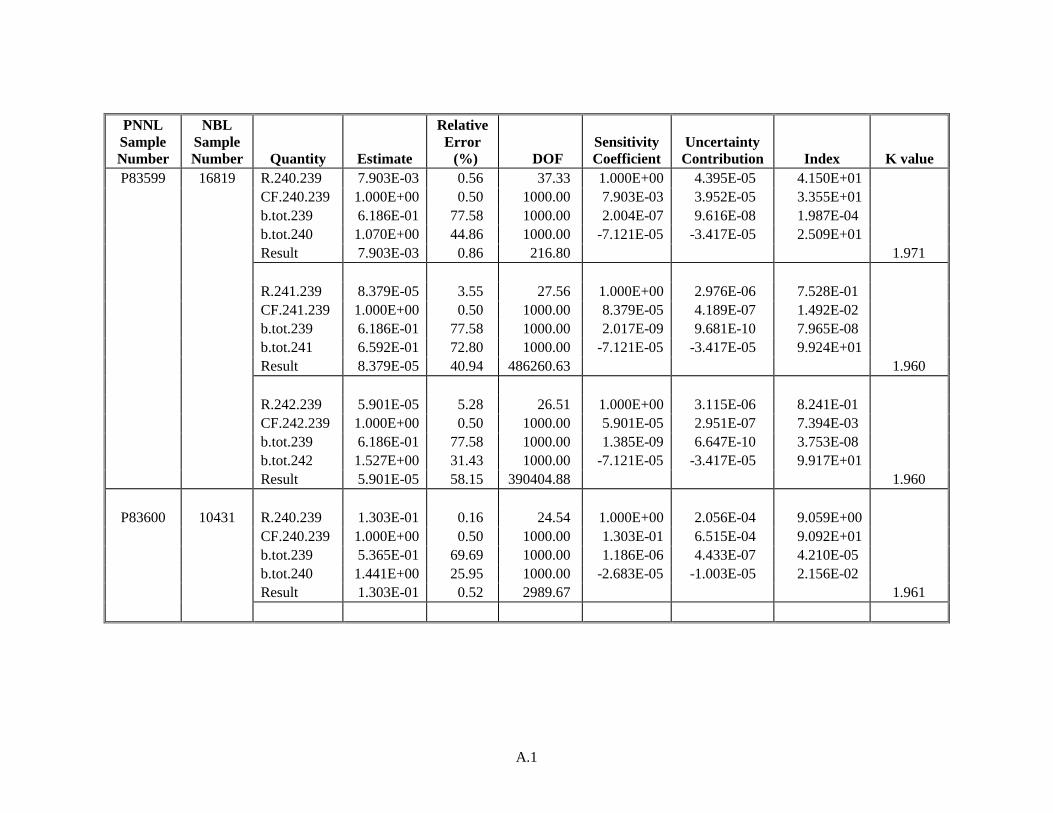
A.1

PNNL

Sample

Number

NBL

Sample

Number Quantity Estimate

Relative

Error

(%) DOF

Sensitivity

Coefficient

Uncertainty


P83599 16819 R.240.239 7.903E-03 0.56 37.33 1.000E+00 4.395E-05 4.150E+01

CF.240.239 1.000E+00 0.50 1000.00 7.903E-03 3.952E-05 3.355E+01

b.tot.239 6.186E-01 77.58 1000.00 2.004E-07 9.616E-08 1.987E-04

b.tot.240 1.070E+00 44.86 1000.00 -7.121E-05 -3.417E-05 2.509E+01

Result 7.903E-03 0.86 216.80 1.971

R.241.239 8.379E-05 3.55 27.56 1.000E+00 2.976E-06 7.528E-01

CF.241.239 1.000E+00 0.50 1000.00 8.379E-05 4.189E-07 1.492E-02

b.tot.239 6.186E-01 77.58 1000.00 2.017E-09 9.681E-10 7.965E-08

b.tot.241 6.592E-01 72.80 1000.00 -7.121E-05 -3.417E-05 9.924E+01

Result 8.379E-05 40.94 486260.63 1.960

R.242.239 5.901E-05 5.28 26.51 1.000E+00 3.115E-06 8.241E-01

CF.242.239 1.000E+00 0.50 1000.00 5.901E-05 2.951E-07 7.394E-03

b.tot.239 6.186E-01 77.58 1000.00 1.385E-09 6.647E-10 3.753E-08

b.tot.242 1.527E+00 31.43 1000.00 -7.121E-05 -3.417E-05 9.917E+01

Result 5.901E-05 58.15 390404.88 1.960

P83600 10431 R.240.239 1.303E-01 0.16 24.54 1.000E+00 2.056E-04 9.059E+00

CF.240.239 1.000E+00 0.50 1000.00 1.303E-01 6.515E-04 9.092E+01

b.tot.239 5.365E-01 69.69 1000.00 1.186E-06 4.433E-07 4.210E-05

b.tot.240 1.441E+00 25.95 1000.00 -2.683E-05 -1.003E-05 2.156E-02

Result 1.303E-01 0.52 2989.67 1.961

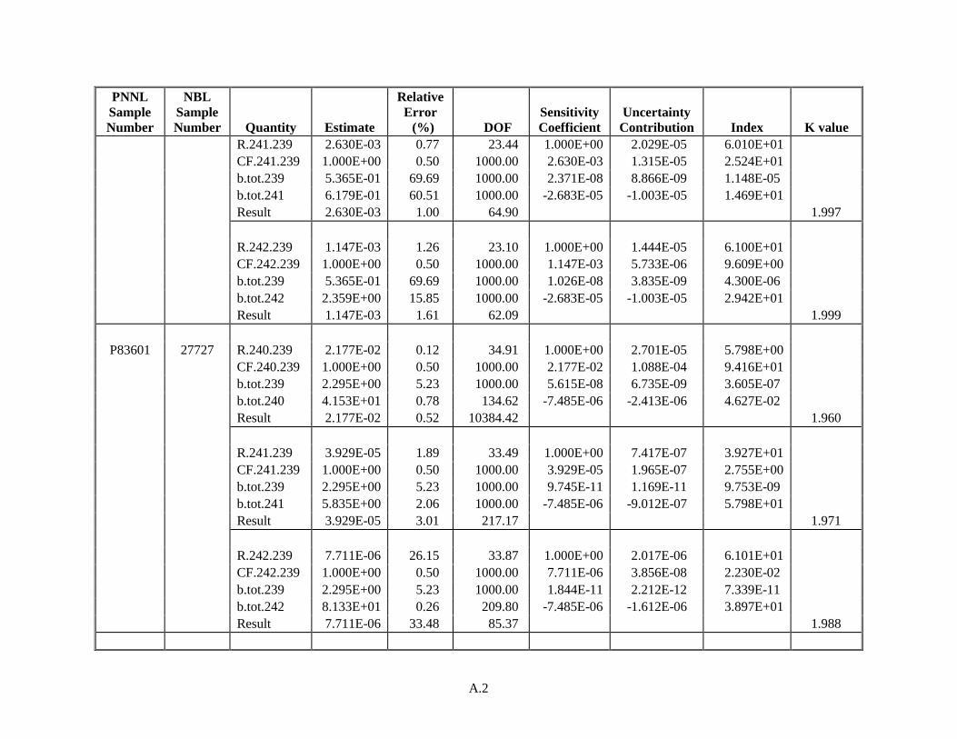
A.2

PNNL

Sample

Number

NBL

Sample


Relative

Error

(%) DOF

Sensitivity

Coefficient

Uncertainty


R.241.239 2.630E-03 0.77 23.44 1.000E+00 2.029E-05 6.010E+01

CF.241.239 1.000E+00 0.50 1000.00 2.630E-03 1.315E-05 2.524E+01

b.tot.239 5.365E-01 69.69 1000.00 2.371E-08 8.866E-09 1.148E-05

b.tot.241 6.179E-01 60.51 1000.00 -2.683E-05 -1.003E-05 1.469E+01

Result 2.630E-03 1.00 64.90 1.997

R.242.239 1.147E-03 1.26 23.10 1.000E+00 1.444E-05 6.100E+01

CF.242.239 1.000E+00 0.50 1000.00 1.147E-03 5.733E-06 9.609E+00

b.tot.239 5.365E-01 69.69 1000.00 1.026E-08 3.835E-09 4.300E-06

b.tot.242 2.359E+00 15.85 1000.00 -2.683E-05 -1.003E-05 2.942E+01

Result 1.147E-03 1.61 62.09 1.999

P83601 27727 R.240.239 2.177E-02 0.12 34.91 1.000E+00 2.701E-05 5.798E+00

CF.240.239 1.000E+00 0.50 1000.00 2.177E-02 1.088E-04 9.416E+01

b.tot.239 2.295E+00 5.23 1000.00 5.615E-08 6.735E-09 3.605E-07

b.tot.240 4.153E+01 0.78 134.62 -7.485E-06 -2.413E-06 4.627E-02

Result 2.177E-02 0.52 10384.42 1.960

R.241.239 3.929E-05 1.89 33.49 1.000E+00 7.417E-07 3.927E+01

CF.241.239 1.000E+00 0.50 1000.00 3.929E-05 1.965E-07 2.755E+00

b.tot.239 2.295E+00 5.23 1000.00 9.745E-11 1.169E-11 9.753E-09

b.tot.241 5.835E+00 2.06 1000.00 -7.485E-06 -9.012E-07 5.798E+01

Result 3.929E-05 3.01 217.17 1.971

R.242.239 7.711E-06 26.15 33.87 1.000E+00 2.017E-06 6.101E+01

CF.242.239 1.000E+00 0.50 1000.00 7.711E-06 3.856E-08 2.230E-02

b.tot.239 2.295E+00 5.23 1000.00 1.844E-11 2.212E-12 7.339E-11

b.tot.242 8.133E+01 0.26 209.80 -7.485E-06 -1.612E-06 3.897E+01

Result 7.711E-06 33.48 85.37 1.988

A.3

PNNL

Sample

Number

NBL

Sample


Relative

Error

(%) DOF

Sensitivity

Coefficient

Uncertainty


P83673 28402 R.240.239 7.433E-02 0.14 45.19 1.000E+00 1.072E-04 7.669E+00

CF.240.239 1.000E+00 0.50 1000.00 7.433E-02 3.716E-04 9.211E+01

b.tot.239 6.246E-01 71.02 1000.00 1.022E-06 4.533E-07 1.370E-04

b.tot.240 1.907E+00 23.27 1000.00 -4.166E-05 -1.848E-05 2.279E-01

Result 7.433E-02 0.52 7684.05 1.960

R.241.239 7.760E-04 4.86 25.44 1.000E+00 3.772E-05 7.997E+01

CF.241.239 1.000E+00 0.50 1000.00 7.760E-04 3.880E-06 8.461E-01

b.tot.239 6.246E-01 71.02 1000.00 1.056E-08 4.684E-09 1.233E-06

b.tot.241 7.409E-01 59.87 1000.00 -4.166E-05 -1.848E-05 1.919E+01

Result 7.760E-04 5.44 39.78 2.021

R.242.239 2.160E-04 1.83 44.13 1.000E+00 3.953E-06 4.361E+00

CF.242.239 1.000E+00 0.50 1000.00 2.160E-04 1.080E-06 3.254E-01

b.tot.239 6.246E-01 71.02 1000.00 2.960E-09 1.313E-09 4.813E-07

b.tot.242 3.217E+00 13.79 1000.00 -4.166E-05 -1.848E-05 9.533E+01

Result 2.160E-04 8.76 23201.22 1.960

P83674.1 44746 R.240.239 1.155E-01 0.40 31.83 1.000E+00 4.564E-04 3.833E+01

CF.240.239 1.000E+00 0.50 1000.00 1.155E-01 5.773E-04 6.134E+01

b.tot.239 3.027E-01 53.08 1000.00 1.039E-05 1.669E-06 5.127E-04

b.tot.240 8.480E-01 18.96 1000.00 -2.740E-04 -4.405E-05 3.571E-01

Result 1.155E-01 0.64 216.67 1.971

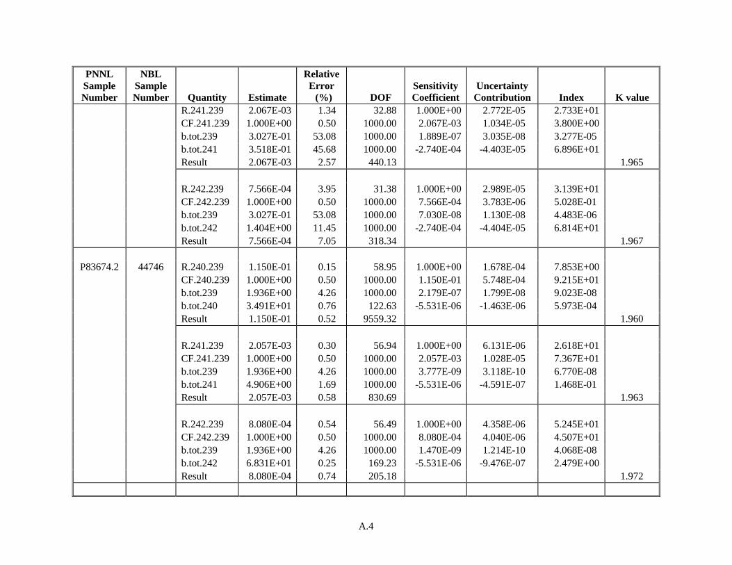
A.4

PNNL

Sample

Number

NBL

Sample


Relative

Error

(%) DOF

Sensitivity

Coefficient

Uncertainty


R.241.239 2.067E-03 1.34 32.88 1.000E+00 2.772E-05 2.733E+01

CF.241.239 1.000E+00 0.50 1000.00 2.067E-03 1.034E-05 3.800E+00

b.tot.239 3.027E-01 53.08 1000.00 1.889E-07 3.035E-08 3.277E-05

b.tot.241 3.518E-01 45.68 1000.00 -2.740E-04 -4.403E-05 6.896E+01

Result 2.067E-03 2.57 440.13 1.965

R.242.239 7.566E-04 3.95 31.38 1.000E+00 2.989E-05 3.139E+01

CF.242.239 1.000E+00 0.50 1000.00 7.566E-04 3.783E-06 5.028E-01

b.tot.239 3.027E-01 53.08 1000.00 7.030E-08 1.130E-08 4.483E-06

b.tot.242 1.404E+00 11.45 1000.00 -2.740E-04 -4.404E-05 6.814E+01

Result 7.566E-04 7.05 318.34 1.967

P83674.2 44746 R.240.239 1.150E-01 0.15 58.95 1.000E+00 1.678E-04 7.853E+00

CF.240.239 1.000E+00 0.50 1000.00 1.150E-01 5.748E-04 9.215E+01

b.tot.239 1.936E+00 4.26 1000.00 2.179E-07 1.799E-08 9.023E-08

b.tot.240 3.491E+01 0.76 122.63 -5.531E-06 -1.463E-06 5.973E-04

Result 1.150E-01 0.52 9559.32 1.960

R.241.239 2.057E-03 0.30 56.94 1.000E+00 6.131E-06 2.618E+01

CF.241.239 1.000E+00 0.50 1000.00 2.057E-03 1.028E-05 7.367E+01

b.tot.239 1.936E+00 4.26 1000.00 3.777E-09 3.118E-10 6.770E-08

b.tot.241 4.906E+00 1.69 1000.00 -5.531E-06 -4.591E-07 1.468E-01

Result 2.057E-03 0.58 830.69 1.963

R.242.239 8.080E-04 0.54 56.49 1.000E+00 4.358E-06 5.245E+01

CF.242.239 1.000E+00 0.50 1000.00 8.080E-04 4.040E-06 4.507E+01

b.tot.239 1.936E+00 4.26 1000.00 1.470E-09 1.214E-10 4.068E-08

b.tot.242 6.831E+01 0.25 169.23 -5.531E-06 -9.476E-07 2.479E+00

Result 8.080E-04 0.74 205.18 1.972

A.5

PNNL

Sample

Number

NBL

Sample


Relative

Error

(%) DOF

Sensitivity

Coefficient

Uncertainty


P83749 37796 R.240.239 8.975E-03 0.70 43.33 1.000E+00 6.258E-05 3.773E+01

CF.240.239 1.000E+00 0.50 1000.00 8.975E-03 4.488E-05 1.940E+01

b.tot.239 4.434E-01 62.40 1000.00 7.165E-07 1.983E-07 3.787E-04

b.tot.240 1.267E+00 21.84 1000.00 -2.417E-04 -6.691E-05 4.312E+01

Result 8.975E-03 1.14 304.38 1.968

R.241.239 2.920E-05 17.29 18.51 1.000E+00 5.049E-06 5.666E-01

CF.241.239 1.000E+00 0.50 1000.00 2.920E-05 1.460E-07 4.736E-04

b.tot.239 4.434E-01 62.40 1000.00 2.159E-09 5.973E-10 7.929E-09

b.tot.241 5.170E-01 53.52 1000.00 -2.417E-04 -6.689E-05 9.943E+01

Result 2.920E-05 229.76 576778.58 1.960

R.242.239 3.013E-05 27.21 35.37 1.000E+00 8.199E-06 1.480E+00

CF.242.239 1.000E+00 0.50 1000.00 3.013E-05 1.507E-07 4.998E-04

b.tot.239 4.434E-01 62.40 1000.00 1.472E-09 4.073E-10 3.652E-09

b.tot.242 2.100E+00 13.18 1000.00 -2.417E-04 -6.690E-05 9.852E+01

Result 3.013E-05 223.65 161496.88 1.960

P84104 UCAR

25-B

R.240.239 1.021E-01 0.09 36.56 1.000E+00 8.767E-05 2.862E+00

CF.240.239 1.000E+00 0.50 1000.00 1.021E-01 5.107E-04 9.712E+01

b.tot.239 8.500E-01 48.39 1000.00 5.483E-07 2.255E-07 1.894E-05

b.tot.240 6.208E+00 6.66 1000.00 -1.614E-05 -6.671E-06 1.657E-02

Result 1.021E-01 0.51 44630.00 1.960

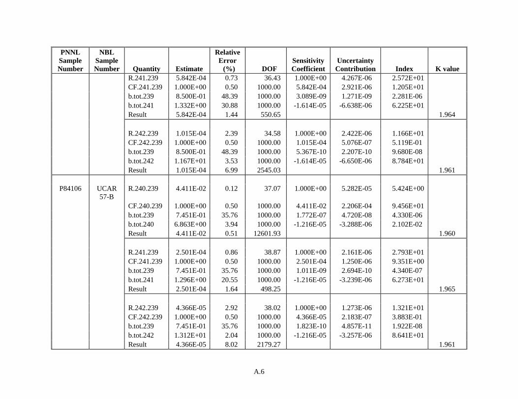
A.6

PNNL

Sample

Number

NBL

Sample


Relative

Error

(%) DOF

Sensitivity

Coefficient

Uncertainty


R.241.239 5.842E-04 0.73 36.43 1.000E+00 4.267E-06 2.572E+01

CF.241.239 1.000E+00 0.50 1000.00 5.842E-04 2.921E-06 1.205E+01

b.tot.239 8.500E-01 48.39 1000.00 3.089E-09 1.271E-09 2.281E-06

b.tot.241 1.332E+00 30.88 1000.00 -1.614E-05 -6.638E-06 6.225E+01

Result 5.842E-04 1.44 550.65 1.964

R.242.239 1.015E-04 2.39 34.58 1.000E+00 2.422E-06 1.166E+01

CF.242.239 1.000E+00 0.50 1000.00 1.015E-04 5.076E-07 5.119E-01

b.tot.239 8.500E-01 48.39 1000.00 5.367E-10 2.207E-10 9.680E-08

b.tot.242 1.167E+01 3.53 1000.00 -1.614E-05 -6.650E-06 8.784E+01

Result 1.015E-04 6.99 2545.03 1.961

P84106 UCAR

57-B

R.240.239 4.411E-02 0.12 37.07 1.000E+00 5.282E-05 5.424E+00

CF.240.239 1.000E+00 0.50 1000.00 4.411E-02 2.206E-04 9.456E+01

b.tot.239 7.451E-01 35.76 1000.00 1.772E-07 4.720E-08 4.330E-06

b.tot.240 6.863E+00 3.94 1000.00 -1.216E-05 -3.288E-06 2.102E-02

Result 4.411E-02 0.51 12601.93 1.960

R.241.239 2.501E-04 0.86 38.87 1.000E+00 2.161E-06 2.793E+01

CF.241.239 1.000E+00 0.50 1000.00 2.501E-04 1.250E-06 9.351E+00

b.tot.239 7.451E-01 35.76 1000.00 1.011E-09 2.694E-10 4.340E-07

b.tot.241 1.296E+00 20.55 1000.00 -1.216E-05 -3.239E-06 6.273E+01

Result 2.501E-04 1.64 498.25 1.965

R.242.239 4.366E-05 2.92 38.02 1.000E+00 1.273E-06 1.321E+01

CF.242.239 1.000E+00 0.50 1000.00 4.366E-05 2.183E-07 3.883E-01

b.tot.239 7.451E-01 35.76 1000.00 1.823E-10 4.857E-11 1.922E-08

b.tot.242 1.312E+01 2.04 1000.00 -1.216E-05 -3.257E-06 8.641E+01

Result 4.366E-05 8.02 2179.27 1.961

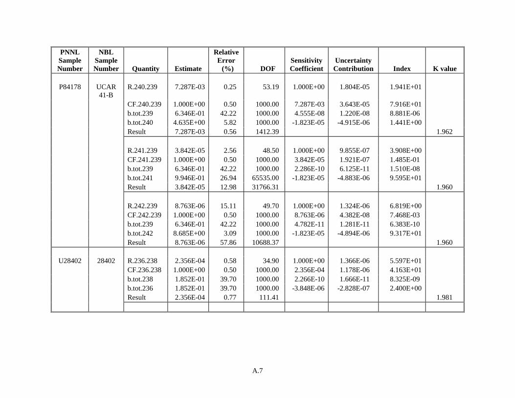
A.7

PNNL

Sample

Number

NBL

Sample


Relative

Error

(%) DOF

Sensitivity

Coefficient

Uncertainty


P84178 UCAR

41-B

R.240.239 7.287E-03 0.25 53.19 1.000E+00 1.804E-05 1.941E+01

CF.240.239 1.000E+00 0.50 1000.00 7.287E-03 3.643E-05 7.916E+01

b.tot.239 6.346E-01 42.22 1000.00 4.555E-08 1.220E-08 8.881E-06

b.tot.240 4.635E+00 5.82 1000.00 -1.823E-05 -4.915E-06 1.441E+00

Result 7.287E-03 0.56 1412.39 1.962

R.241.239 3.842E-05 2.56 48.50 1.000E+00 9.855E-07 3.908E+00

CF.241.239 1.000E+00 0.50 1000.00 3.842E-05 1.921E-07 1.485E-01

b.tot.239 6.346E-01 42.22 1000.00 2.286E-10 6.125E-11 1.510E-08

b.tot.241 9.946E-01 26.94 65535.00 -1.823E-05 -4.883E-06 9.595E+01

Result 3.842E-05 12.98 31766.31 1.960

R.242.239 8.763E-06 15.11 49.70 1.000E+00 1.324E-06 6.819E+00

CF.242.239 1.000E+00 0.50 1000.00 8.763E-06 4.382E-08 7.468E-03

b.tot.239 6.346E-01 42.22 1000.00 4.782E-11 1.281E-11 6.383E-10

b.tot.242 8.685E+00 3.09 1000.00 -1.823E-05 -4.894E-06 9.317E+01

Result 8.763E-06 57.86 10688.37 1.960

U28402 28402 R.236.238 2.356E-04 0.58 34.90 1.000E+00 1.366E-06 5.597E+01

CF.236.238 1.000E+00 0.50 1000.00 2.356E-04 1.178E-06 4.163E+01

b.tot.238 1.852E-01 39.70 1000.00 2.266E-10 1.666E-11 8.325E-09

b.tot.236 1.852E-01 39.70 1000.00 -3.848E-06 -2.828E-07 2.400E+00

Result 2.356E-04 0.77 111.41 1.981

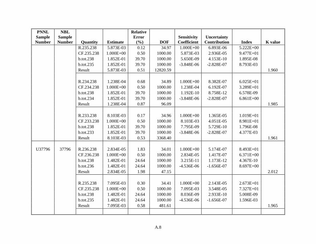
A.8

PNNL

Sample

Number

NBL

Sample


Relative

Error

(%) DOF

Sensitivity

Coefficient

Uncertainty


R.235.238 5.873E-03 0.12 34.97 1.000E+00 6.893E-06 5.222E+00

CF.235.238 1.000E+00 0.50 1000.00 5.873E-03 2.936E-05 9.477E+01

b.tot.238 1.852E-01 39.70 1000.00 5.650E-09 4.153E-10 1.895E-08

b.tot.235 1.852E-01 39.70 1000.00 -3.848E-06 -2.828E-07 8.793E-03

Result 5.873E-03 0.51 12820.59 1.960

R.234.238 1.238E-04 0.68 34.89 1.000E+00 8.382E-07 6.025E+01

CF.234.238 1.000E+00 0.50 1000.00 1.238E-04 6.192E-07 3.289E+01

b.tot.238 1.852E-01 39.70 1000.00 1.192E-10 8.758E-12 6.578E-09

b.tot.234 1.852E-01 39.70 1000.00 -3.848E-06 -2.828E-07 6.861E+00

Result 1.238E-04 0.87 96.09 1.985

R.233.238 8.103E-03 0.17 34.96 1.000E+00 1.365E-05 1.019E+01

CF.233.238 1.000E+00 0.50 1000.00 8.103E-03 4.051E-05 8.981E+01

b.tot.238 1.852E-01 39.70 1000.00 7.795E-09 5.729E-10 1.796E-08

b.tot.233 1.852E-01 39.70 1000.00 -3.848E-06 -2.828E-07 4.377E-03

Result 8.103E-03 0.53 3368.40 1.961

U37796 37796 R.236.238 2.834E-05 1.83 34.01 1.000E+00 5.174E-07 8.493E+01

CF.236.238 1.000E+00 0.50 1000.00 2.834E-05 1.417E-07 6.371E+00

b.tot.238 1.482E-01 24.64 1000.00 3.215E-11 1.173E-12 4.367E-10

b.tot.236 1.482E-01 24.64 1000.00 -4.536E-06 -1.656E-07 8.697E+00

Result 2.834E-05 1.98 47.15 2.012

R.235.238 7.095E-03 0.30 34.41 1.000E+00 2.143E-05 2.673E+01

CF.235.238 1.000E+00 0.50 1000.00 7.095E-03 3.548E-05 7.327E+01

b.tot.238 1.482E-01 24.64 1000.00 8.036E-09 2.933E-10 5.008E-09

b.tot.235 1.482E-01 24.64 1000.00 -4.536E-06 -1.656E-07 1.596E-03

Result 7.095E-03 0.58 481.61 1.965

A.9

PNNL

Sample

Number

NBL

Sample


Relative

Error

(%) DOF

Sensitivity

Coefficient

Uncertainty


R.234.238 6.118E-05 0.99 34.33 1.000E+00 6.064E-07 7.525E+01

CF.234.238 1.000E+00 0.50 1000.00 6.118E-05 3.059E-07 1.915E+01

b.tot.238 1.482E-01 24.64 1000.00 6.930E-11 2.529E-12 1.309E-09

b.tot.234 1.482E-01 24.64 1000.00 -4.536E-06 -1.656E-07 5.609E+00

Result 6.118E-05 1.14 60.63 2.000

R.233.238 9.190E-04 0.37 34.38 1.000E+00 3.365E-06 3.488E+01

CF.233.238 1.000E+00 0.50 1000.00 9.190E-04 4.595E-06 6.503E+01

b.tot.238 1.482E-01 24.64 1000.00 1.040E-09 3.797E-11 4.441E-09

b.tot.233 1.482E-01 24.64 1000.00 -4.536E-06 -1.656E-07 8.444E-02

Result 9.190E-04 0.62 282.54 1.968

U44746 44746 R.236.238 3.055E-04 1.06 22.43 1.000E+00 3.252E-06 8.181E+01

CF.236.238 1.000E+00 0.50 1000.00 3.055E-04 1.527E-06 1.805E+01

b.tot.238 1.389E-01 19.59 1000.00 3.817E-10 1.038E-11 8.340E-10

b.tot.236 1.389E-01 19.59 1000.00 -5.005E-06 -1.361E-07 1.434E-01

Result 3.055E-04 1.18 33.52 2.033

R.235.238 5.481E-03 0.55 22.42 1.000E+00 3.035E-05 5.508E+01

CF.235.238 1.000E+00 0.50 1000.00 5.481E-03 2.741E-05 4.492E+01

b.tot.238 1.389E-01 19.59 1000.00 6.853E-09 1.864E-10 2.078E-09

b.tot.235 1.389E-01 19.59 1000.00 -5.005E-06 -1.361E-07 1.108E-03

Result 5.481E-03 0.75 73.89 1.993

R.234.238 2.796E-04 0.66 22.46 1.000E+00 1.856E-06 6.359E+01

CF.234.238 1.000E+00 0.50 1000.00 2.796E-04 1.398E-06 3.607E+01

b.tot.238 1.389E-01 19.59 1000.00 3.495E-10 9.505E-12 1.667E-09

b.tot.234 1.389E-01 19.59 1000.00 -5.005E-06 -1.361E-07 3.420E-01

Result 2.796E-04 0.83 55.56 2.004

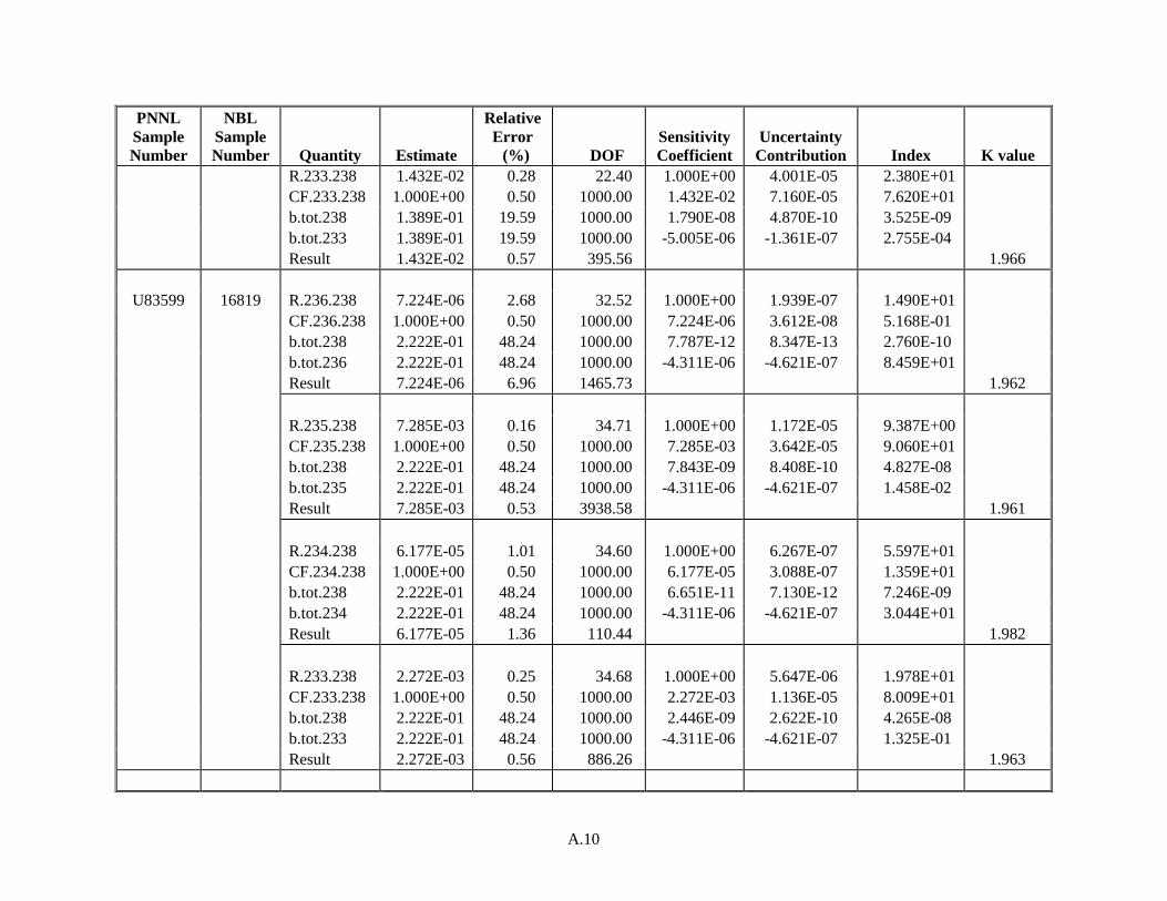
A.10

PNNL

Sample

Number

NBL

Sample


Relative

Error

(%) DOF

Sensitivity

Coefficient

Uncertainty


R.233.238 1.432E-02 0.28 22.40 1.000E+00 4.001E-05 2.380E+01

CF.233.238 1.000E+00 0.50 1000.00 1.432E-02 7.160E-05 7.620E+01

b.tot.238 1.389E-01 19.59 1000.00 1.790E-08 4.870E-10 3.525E-09

b.tot.233 1.389E-01 19.59 1000.00 -5.005E-06 -1.361E-07 2.755E-04

Result 1.432E-02 0.57 395.56 1.966

U83599 16819 R.236.238 7.224E-06 2.68 32.52 1.000E+00 1.939E-07 1.490E+01

CF.236.238 1.000E+00 0.50 1000.00 7.224E-06 3.612E-08 5.168E-01

b.tot.238 2.222E-01 48.24 1000.00 7.787E-12 8.347E-13 2.760E-10

b.tot.236 2.222E-01 48.24 1000.00 -4.311E-06 -4.621E-07 8.459E+01

Result 7.224E-06 6.96 1465.73 1.962

R.235.238 7.285E-03 0.16 34.71 1.000E+00 1.172E-05 9.387E+00

CF.235.238 1.000E+00 0.50 1000.00 7.285E-03 3.642E-05 9.060E+01

b.tot.238 2.222E-01 48.24 1000.00 7.843E-09 8.408E-10 4.827E-08

b.tot.235 2.222E-01 48.24 1000.00 -4.311E-06 -4.621E-07 1.458E-02

Result 7.285E-03 0.53 3938.58 1.961

R.234.238 6.177E-05 1.01 34.60 1.000E+00 6.267E-07 5.597E+01

CF.234.238 1.000E+00 0.50 1000.00 6.177E-05 3.088E-07 1.359E+01

b.tot.238 2.222E-01 48.24 1000.00 6.651E-11 7.130E-12 7.246E-09

b.tot.234 2.222E-01 48.24 1000.00 -4.311E-06 -4.621E-07 3.044E+01

Result 6.177E-05 1.36 110.44 1.982

R.233.238 2.272E-03 0.25 34.68 1.000E+00 5.647E-06 1.978E+01

CF.233.238 1.000E+00 0.50 1000.00 2.272E-03 1.136E-05 8.009E+01

b.tot.238 2.222E-01 48.24 1000.00 2.446E-09 2.622E-10 4.265E-08

b.tot.233 2.222E-01 48.24 1000.00 -4.311E-06 -4.621E-07 1.325E-01

Result 2.272E-03 0.56 886.26 1.963

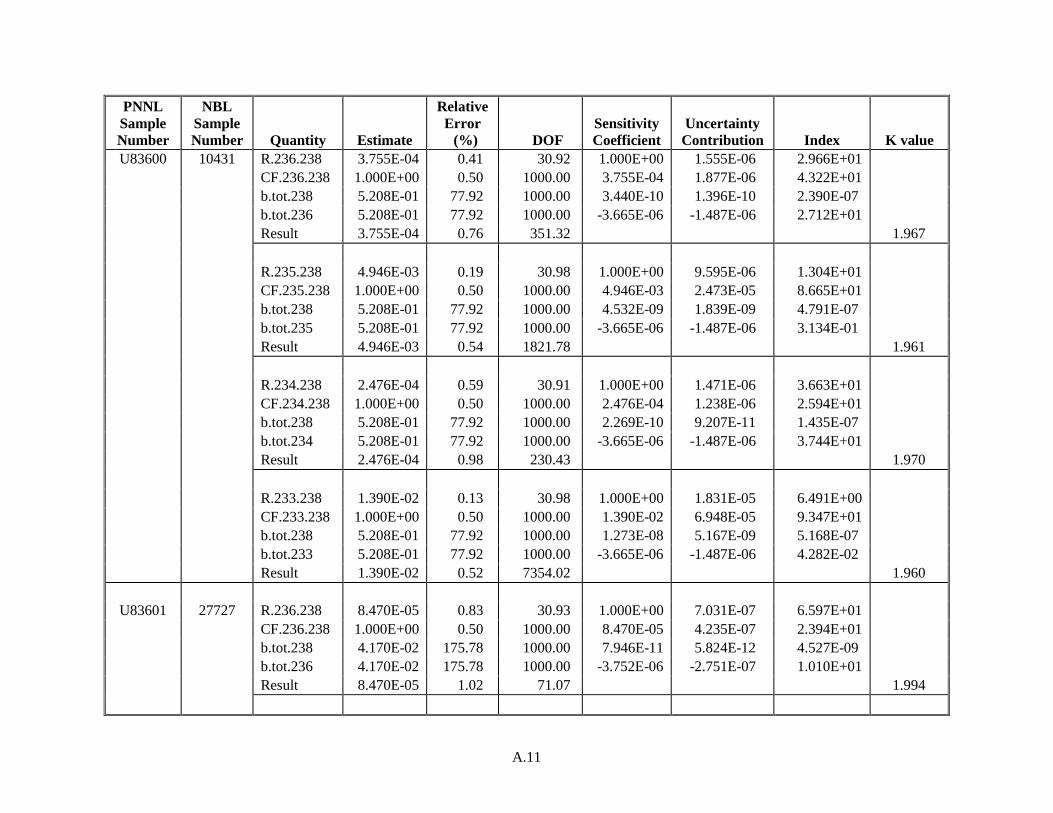
A.11

PNNL

Sample

Number

NBL

Sample


Relative

Error

(%) DOF

Sensitivity

Coefficient

Uncertainty


U83600 10431 R.236.238 3.755E-04 0.41 30.92 1.000E+00 1.555E-06 2.966E+01

CF.236.238 1.000E+00 0.50 1000.00 3.755E-04 1.877E-06 4.322E+01

b.tot.238 5.208E-01 77.92 1000.00 3.440E-10 1.396E-10 2.390E-07

b.tot.236 5.208E-01 77.92 1000.00 -3.665E-06 -1.487E-06 2.712E+01

Result 3.755E-04 0.76 351.32 1.967

R.235.238 4.946E-03 0.19 30.98 1.000E+00 9.595E-06 1.304E+01

CF.235.238 1.000E+00 0.50 1000.00 4.946E-03 2.473E-05 8.665E+01

b.tot.238 5.208E-01 77.92 1000.00 4.532E-09 1.839E-09 4.791E-07

b.tot.235 5.208E-01 77.92 1000.00 -3.665E-06 -1.487E-06 3.134E-01

Result 4.946E-03 0.54 1821.78 1.961

R.234.238 2.476E-04 0.59 30.91 1.000E+00 1.471E-06 3.663E+01

CF.234.238 1.000E+00 0.50 1000.00 2.476E-04 1.238E-06 2.594E+01

b.tot.238 5.208E-01 77.92 1000.00 2.269E-10 9.207E-11 1.435E-07

b.tot.234 5.208E-01 77.92 1000.00 -3.665E-06 -1.487E-06 3.744E+01

Result 2.476E-04 0.98 230.43 1.970

R.233.238 1.390E-02 0.13 30.98 1.000E+00 1.831E-05 6.491E+00

CF.233.238 1.000E+00 0.50 1000.00 1.390E-02 6.948E-05 9.347E+01

b.tot.238 5.208E-01 77.92 1000.00 1.273E-08 5.167E-09 5.168E-07

b.tot.233 5.208E-01 77.92 1000.00 -3.665E-06 -1.487E-06 4.282E-02

Result 1.390E-02 0.52 7354.02 1.960

U83601 27727 R.236.238 8.470E-05 0.83 30.93 1.000E+00 7.031E-07 6.597E+01

CF.236.238 1.000E+00 0.50 1000.00 8.470E-05 4.235E-07 2.394E+01

b.tot.238 4.170E-02 175.78 1000.00 7.946E-11 5.824E-12 4.527E-09

b.tot.236 4.170E-02 175.78 1000.00 -3.752E-06 -2.751E-07 1.010E+01

Result 8.470E-05 1.02 71.07 1.994

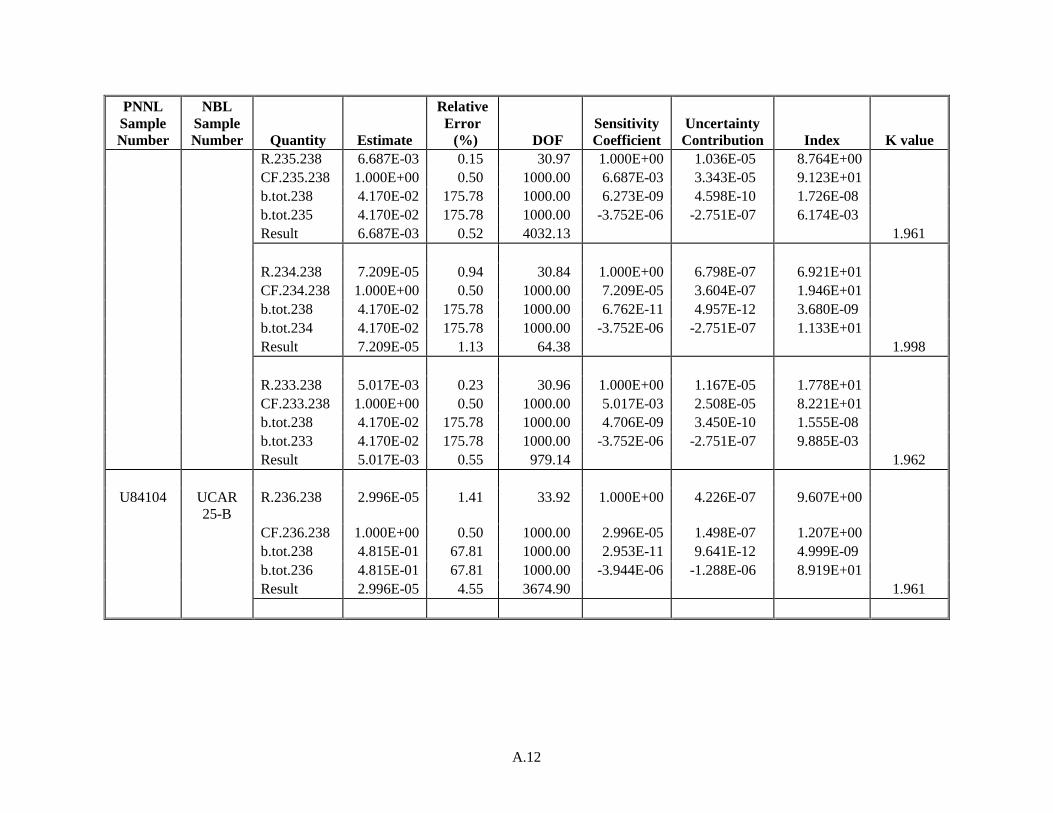
A.12

PNNL

Sample

Number

NBL

Sample


Relative

Error

(%) DOF

Sensitivity

Coefficient

Uncertainty


R.235.238 6.687E-03 0.15 30.97 1.000E+00 1.036E-05 8.764E+00

CF.235.238 1.000E+00 0.50 1000.00 6.687E-03 3.343E-05 9.123E+01

b.tot.238 4.170E-02 175.78 1000.00 6.273E-09 4.598E-10 1.726E-08

b.tot.235 4.170E-02 175.78 1000.00 -3.752E-06 -2.751E-07 6.174E-03

Result 6.687E-03 0.52 4032.13 1.961

R.234.238 7.209E-05 0.94 30.84 1.000E+00 6.798E-07 6.921E+01

CF.234.238 1.000E+00 0.50 1000.00 7.209E-05 3.604E-07 1.946E+01

b.tot.238 4.170E-02 175.78 1000.00 6.762E-11 4.957E-12 3.680E-09

b.tot.234 4.170E-02 175.78 1000.00 -3.752E-06 -2.751E-07 1.133E+01

Result 7.209E-05 1.13 64.38 1.998

R.233.238 5.017E-03 0.23 30.96 1.000E+00 1.167E-05 1.778E+01

CF.233.238 1.000E+00 0.50 1000.00 5.017E-03 2.508E-05 8.221E+01

b.tot.238 4.170E-02 175.78 1000.00 4.706E-09 3.450E-10 1.555E-08

b.tot.233 4.170E-02 175.78 1000.00 -3.752E-06 -2.751E-07 9.885E-03

Result 5.017E-03 0.55 979.14 1.962

U84104 UCAR

25-B

R.236.238 2.996E-05 1.41 33.92 1.000E+00 4.226E-07 9.607E+00

CF.236.238 1.000E+00 0.50 1000.00 2.996E-05 1.498E-07 1.207E+00

b.tot.238 4.815E-01 67.81 1000.00 2.953E-11 9.641E-12 4.999E-09

b.tot.236 4.815E-01 67.81 1000.00 -3.944E-06 -1.288E-06 8.919E+01

Result 2.996E-05 4.55 3674.90 1.961

A.13

PNNL

Sample

Number

NBL

Sample


Relative

Error

(%) DOF

Sensitivity

Coefficient

Uncertainty


R.235.238 5.748E-03 0.23 34.93 1.000E+00 1.347E-05 1.798E+01

CF.235.238 1.000E+00 0.50 1000.00 5.748E-03 2.874E-05 8.185E+01

b.tot.238 4.815E-01 67.81 1000.00 5.670E-09 1.851E-09 3.397E-07

b.tot.235 4.815E-01 67.81 1000.00 -3.944E-06 -1.288E-06 1.643E-01

Result 5.748E-03 0.55 1079.97 1.962

R.234.238 3.377E-05 1.19 34.32 1.000E+00 4.027E-07 8.773E+00

CF.234.238 1.000E+00 0.50 1000.00 3.377E-05 1.688E-07 1.542E+00

b.tot.238 4.815E-01 67.81 1000.00 3.328E-11 1.087E-11 6.387E-09

b.tot.234 4.815E-01 67.81 1000.00 -3.944E-06 -1.288E-06 8.969E+01

Result 3.377E-05 4.03 4458.71 1.960

R.233.238 4.391E-04 0.54 34.89 1.000E+00 2.357E-06 4.617E+01

CF.233.238 1.000E+00 0.50 1000.00 4.391E-04 2.195E-06 4.005E+01

b.tot.238 4.815E-01 67.81 1000.00 4.331E-10 1.414E-10 1.662E-07

b.tot.233 4.815E-01 67.81 1000.00 -3.944E-06 -1.288E-06 1.378E+01

Result 4.391E-04 0.79 163.68 1.975

U84105 UCAR

41-B

R.236.238 1.528E-05 8.09 11.54 1.000E+00 1.236E-06 7.867E+01

CF.236.238 1.000E+00 0.50 1000.00 1.528E-05 7.640E-08 3.005E-01

b.tot.238 2.963E-01 47.69 1000.00 1.739E-11 2.458E-12 3.110E-10

b.tot.236 2.963E-01 47.69 1000.00 -4.523E-06 -6.391E-07 2.103E+01

Result 1.528E-05 9.12 18.64 2.096

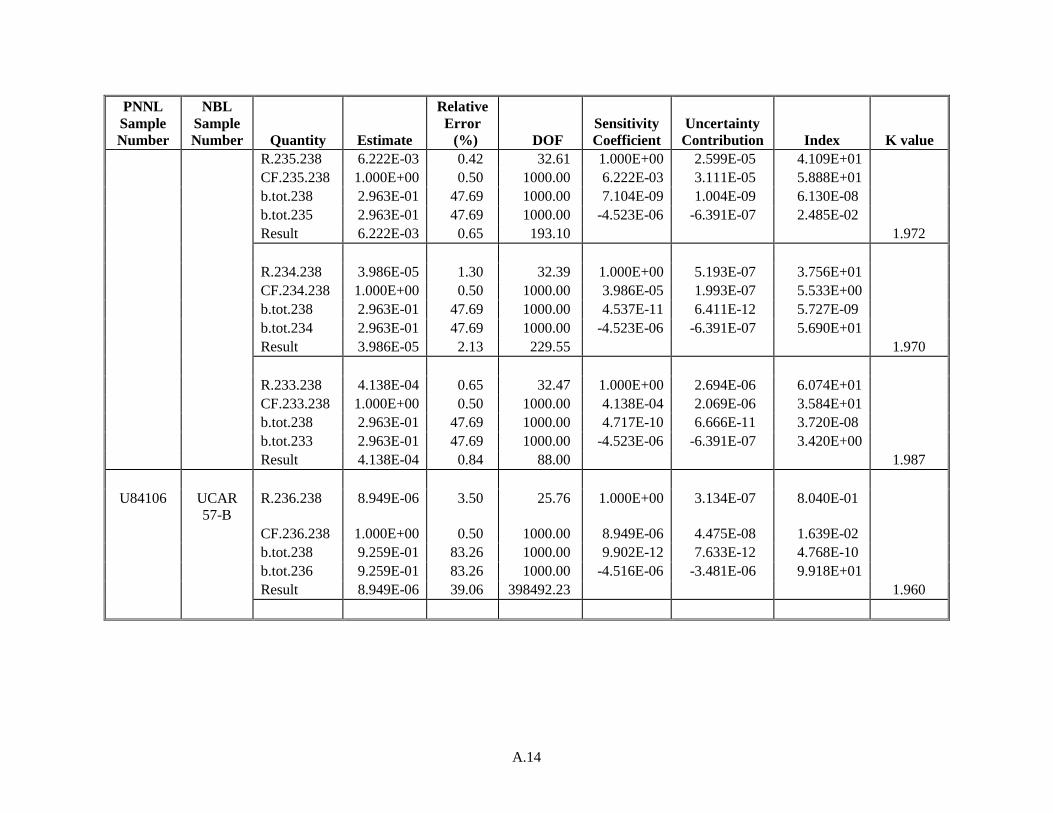
A.14

PNNL

Sample

Number

NBL

Sample


Relative

Error

(%) DOF

Sensitivity

Coefficient

Uncertainty


R.235.238 6.222E-03 0.42 32.61 1.000E+00 2.599E-05 4.109E+01

CF.235.238 1.000E+00 0.50 1000.00 6.222E-03 3.111E-05 5.888E+01

b.tot.238 2.963E-01 47.69 1000.00 7.104E-09 1.004E-09 6.130E-08

b.tot.235 2.963E-01 47.69 1000.00 -4.523E-06 -6.391E-07 2.485E-02

Result 6.222E-03 0.65 193.10 1.972

R.234.238 3.986E-05 1.30 32.39 1.000E+00 5.193E-07 3.756E+01

CF.234.238 1.000E+00 0.50 1000.00 3.986E-05 1.993E-07 5.533E+00

b.tot.238 2.963E-01 47.69 1000.00 4.537E-11 6.411E-12 5.727E-09

b.tot.234 2.963E-01 47.69 1000.00 -4.523E-06 -6.391E-07 5.690E+01

Result 3.986E-05 2.13 229.55 1.970

R.233.238 4.138E-04 0.65 32.47 1.000E+00 2.694E-06 6.074E+01

CF.233.238 1.000E+00 0.50 1000.00 4.138E-04 2.069E-06 3.584E+01

b.tot.238 2.963E-01 47.69 1000.00 4.717E-10 6.666E-11 3.720E-08

b.tot.233 2.963E-01 47.69 1000.00 -4.523E-06 -6.391E-07 3.420E+00

Result 4.138E-04 0.84 88.00 1.987

U84106 UCAR

57-B

R.236.238 8.949E-06 3.50 25.76 1.000E+00 3.134E-07 8.040E-01

CF.236.238 1.000E+00 0.50 1000.00 8.949E-06 4.475E-08 1.639E-02

b.tot.238 9.259E-01 83.26 1000.00 9.902E-12 7.633E-12 4.768E-10

b.tot.236 9.259E-01 83.26 1000.00 -4.516E-06 -3.481E-06 9.918E+01

Result 8.949E-06 39.06 398492.23 1.960

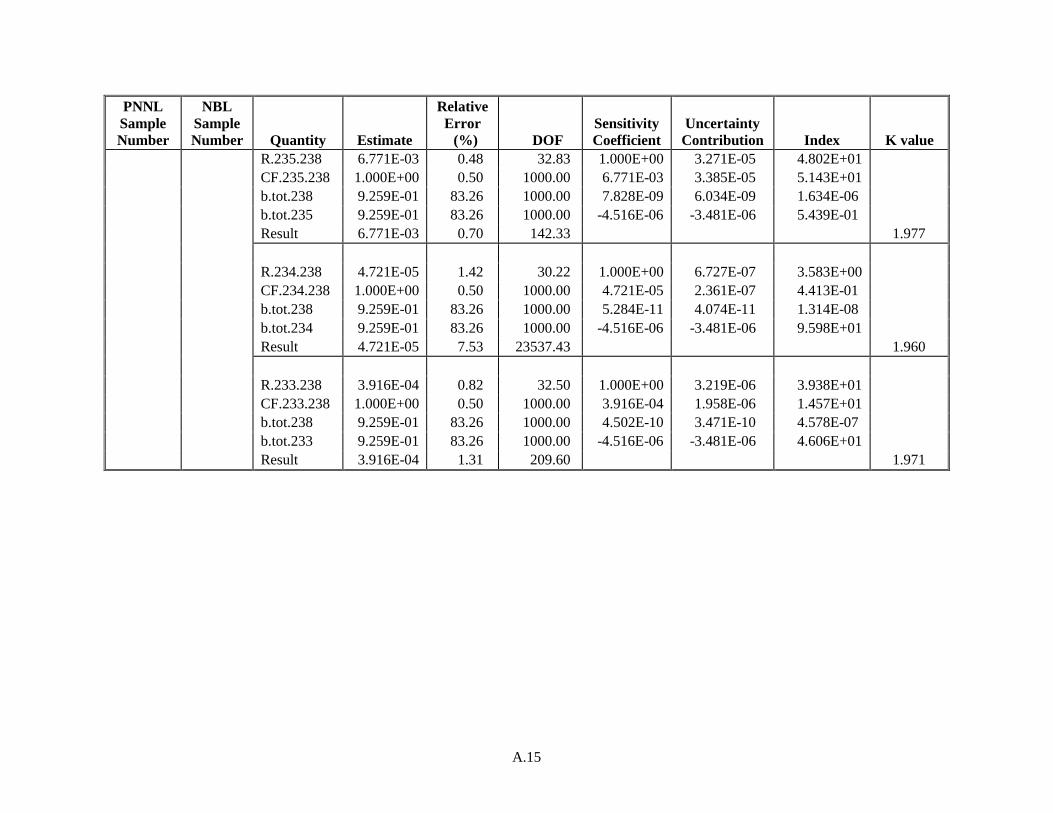
A.15

PNNL

Sample

Number

NBL

Sample


Relative

Error

(%) DOF

Sensitivity

Coefficient

Uncertainty


R.235.238 6.771E-03 0.48 32.83 1.000E+00 3.271E-05 4.802E+01

CF.235.238 1.000E+00 0.50 1000.00 6.771E-03 3.385E-05 5.143E+01

b.tot.238 9.259E-01 83.26 1000.00 7.828E-09 6.034E-09 1.634E-06

b.tot.235 9.259E-01 83.26 1000.00 -4.516E-06 -3.481E-06 5.439E-01

Result 6.771E-03 0.70 142.33 1.977

R.234.238 4.721E-05 1.42 30.22 1.000E+00 6.727E-07 3.583E+00

CF.234.238 1.000E+00 0.50 1000.00 4.721E-05 2.361E-07 4.413E-01

b.tot.238 9.259E-01 83.26 1000.00 5.284E-11 4.074E-11 1.314E-08

b.tot.234 9.259E-01 83.26 1000.00 -4.516E-06 -3.481E-06 9.598E+01

Result 4.721E-05 7.53 23537.43 1.960

R.233.238 3.916E-04 0.82 32.50 1.000E+00 3.219E-06 3.938E+01

CF.233.238 1.000E+00 0.50 1000.00 3.916E-04 1.958E-06 1.457E+01

b.tot.238 9.259E-01 83.26 1000.00 4.502E-10 3.471E-10 4.578E-07

b.tot.233 9.259E-01 83.26 1000.00 -4.516E-06 -3.481E-06 4.606E+01

Result 3.916E-04 1.31 209.60 1.971

gum analysis for tims and sims isotopic ratios in graphite · pnnl-17036 . gum analysis for tims...

Documents