guujkmf
DESCRIPTION
341211wfatrTRANSCRIPT

THE REPUBLIC OF TURKEY
BAHÇEŞEHİR UNIVERSITY
GRADUATE SCHOOL OF
NATURAL AND APPLIED SCIENCES
COMPUTER ENGINEERING
SMART TRANSPORTATION SYSTEMS
Master’s Thesis
NECATİ KILIÇ
Thesis Advisor: ASSOC. PROF. TAŞKIN KOÇAK, PHD.
İSTANBUL, 2012

THE REPUBLIC OF TURKEY
BAHÇEŞEHİR UNIVERSITY
GRADUATE SCHOOL OF NATURAL AND APPLIED SCIENCES
COMPUTER ENGINEERING
Name of the thesis: Smart Transportation Systems
Name/Last Name of the Student: Necati Kılıç
Date of the Defense of Thesis: 15.06.2012
The thesis has been approved by the Graduate School of Natural and Applied Sciences.
Assoc. Prof., Tunç BOZBURA
Graduate School Director
Signature
I certify that this thesis meets all the requirements as a thesis for the degree of Master of
Science.
Asst. Prof., V. Çağrı GÜNGÖR
Program Coordinator
Signature
This is to certify that we have read this thesis and we find it fully adequate in scope,
quality and content, as a thesis for the degree of Master of Science.
Examining Comittee Members Signature____
Thesis Supervisor
Assoc. Prof., Taşkın KOÇAK -----------------------------------
Member
Assoc. Prof., Adem KARAHOCA -----------------------------------
Member
Asst. Prof., K. Egemen ÖZDEN -----------------------------------

ACKNOWLEDGEMENTS
First and foremost, I offer my sincerest gratitude to my advisor, Assoc. Prof. Taşkın
Koçak and my co-advisor Asst. Prof. V. Çağrı Güngör for their visionary support,
enlightening guidance, and patience throughout my thesis. I attribute the level of my
Masters degree to their encouragement and effort and without them this thesis, too,
would not have been completed or written. One simply could not wish for better or
friendlier supervisors.
Besides my advisors, I would like to thank the rest of my thesis committee: Assoc. Prof.
Adem Karahoca, Asst. Prof. Kemal Egemen Özden for their encouragement and
insightful comments.
Moreover, I am deeply grateful to my family and friends Duygu Şahin, Savaş Keskiner,
and Oğuz Şakar for their immense social support and motivation throughout the thesis.
In addition, I offer my special thanks to all those who took trouble to assist me, namely
my researcher friends Mustafa Kapdan, Sevgi Kaya, Ceyhun Can Ülker, Ertunç Erdil,
Selçuk Keskin, Mustafa Kemal Korkmaz, Dilan Şahin, Anıl Üstel, Melike Yiğit, Efsun
Karaca, Hacer Özge Demir and Davut Özcan throughout the research and the
documentation of my thesis.
This work was supported by Türk Telekom Group R&D under Award Number 11316-
02. Additional thanks to Türk Telekom R&D University Collaborations team for their
great support.

iv
ABSTRACT
SMART TRANSPORTATION SYSTEMS
Necati Kılıç
Graduate School of Natural and Applied Sciences
Computer Engineering
Thesis Supervisor: Assoc. Prof. Taşkın Koçak
Co-Supervisor: Asst. Prof. V. Çağrı Güngör
June 2012, 192 pages
Smart or intelligent transportation systems (ITS) have been around for some time.
However, they are re-emerging again with the recent advances in wireless
communications. This is made possible not only by the technological breakthroughs but
also the widespread usage and affordability of the mobile communications based
services. Contrary to the longevity of the experiences in ITS technologies, the road
traffic in metropolitan areas is far cry from acceptable levels.
In order to have a deeper understanding of the aforementioned problem, the state-of-the-
art in smart transportation systems has been studied. Many solutions in the literature that
are offered by the range of top telecom companies, municipalities, corporations,
universities and EU funded projects are reviewed. Communication technologies used in
these solutions are discussed. A wide range of simulation tools in the literature are
investigated which helped us choosing the right set of simulation tools.
The thesis covers the traffic theory background in detail that is investigated in this
project. The meaning and the importance of several parameters which are common in all
traffic applications such as density, flow, speed, gap, etc. are introduced. The
relationship between flow, density and velocity is given and its significance is stated.
The thesis also explored the mathematical traffic flow models that are widely mentioned
in the traffic engineering discipline and are listed in two categories, namely
Macroscopic and Microscopic traffic flow models. A segmented freeway system is
simulated with several macroscopic traffic flow models introduced by Lighthill-
Whitham-Richards, Payne, Papageorgiou and Daganzo. Some of the simulation results
corresponding to Payne and Daganzo’s Cell Transmission Model (CTM) which both
utilize the hydrodynamic theory are given in the thesis. The fundamental diagram which
is a significant concept that is used in both macroscopic and microscopic levels of
traffic flow is studied, as well.
The thesis primarily focused on two steps to address the undying issue of recent decades
which has lately become even more irritating. The first step described our efforts to
construct and introduce a short-term prediction system. A simple yet effective

v
simulation tool called CTMsim is presented. Two different case studies modeling a
portion of TEM freeway ranging from Kavacık to Maslak have been carried out to
demonstrate the abilities of the tool. Firstly, a traffic accident scenario is depicted and
its effects both visually and statistically are displayed in the area of influence. In
addition to it, second scenario interpreted and portrayed the prediction of the traffic
states fifteen minute ahead of time which resulted in a slight difference from the real-
time calculation. Briefly, the tool has been able to capture the traffic dynamics and
present promising results.
The second step is comprised of presenting a real-time traffic monitoring system. On
this sense, a simulator named BAU Traffic Simulator that is integrated with a
smartphone application called TTraffic is developed from the scratch. The tool achieved
to dynamically interpret the outputs of the client (android app) and represent the system
in real-time. The outputs of the simulator can be fetched by the clients in order to get
real-time traffic information, and hence calculate a dynamic routing plan to get to the
destination within the possible minimum time. All analyses carried out during the
development phase are presented in the thesis. Lastly three traffic scenarios simulating
Regular Traffic, Free Flow Traffic, and Traffic Accident conditions are presented and
analyzed thoroughly.
Keywords: Intelligent Transportation Systems, Microscopic Traffic Simulator, Traffic
Prediction, GPS-based Traffic Estimation, Real-time Traffic monitoring

vi
ÖZET
AKILLI ULAŞIM SİSTEMLERİ
Necati Kılıç
Fen Bilimleri Enstitüsü
Bilgisayar Mühendisliği
Tez Danışmanı: Doç. Dr. Taşkın Koçak
Tez İkinci Danışmanı: Yrd. Doç. Dr. V. Çağrı Güngör
Haziran 2012, 192 sayfa
Akıllı Ulaşım Sistemleri bir süredir araştırmacıların gözde konularından biri olarak
çalışılmıştır. Ancak son zamanlarda özellikle kablosuz iletişim sistemlerinde
gerçekleşen teknolojik gelişmeler bu çalışmalara son derece büyük bir hız
kazandırmıştır. Gün geçtikçe ulaşımı kolaylaşan GPS sistemlerinin araçlarda bulunmaya
başlaması ve öte yandan da akıllı cep telefonlarında bu iletişim sistemlerinin entegre
halinde son kullanıcıya kadar ulaşması, gerçek zamanlı trafik bilgisi çıkarımını,
izlenmesini ve tahmin edilebilmesine olanak tanımıştır.
Bu araştırma tezi GPS tabanlı akıllı telefonlar aracılığıyla gerçek zamanlı trafik izleme
ve bilgilendirme sistemlerini ve yakın gelecek zamanlı trafik tahminlerini konu
almaktadır. Araştırma sonunda on beş dakikalık kısa zamanlı tahminler yürütebilen bir
sistemin yanı sıra cep telefonlarından gelen GPS bilgilerini yorumlayabilen bir
simülatör geliştirilmiştir.
Anahtar kelimeler: Akıllı Ulaşım Sistemleri, Mikroskopik Trafik Simülatörü, Kısa
süreli trafik tahmini, GPS tabanlı trafik durumu, Gerçek zamanlı trafik denetimi

vii
CONTENTS
TABLES ......................................................................................................................... xii
FIGURES ...................................................................................................................... xiii
ABBREVIATIONS ...................................................................................................... xix
SYMBOLS…. ................................................................................................................ xx
1. INTRODUCTION ....................................................................................................... 1
1.1 CHALLENGES VS. OPPORTUNITIES ...................................................... 4
1.2 PROPOSED SYSTEM ARCHITECTURE .................................................. 7
2. STATE-OF-THE-ART IN SMART TRANSPORTATION SYSTEMS ................ 8
2.1 TRAFFIC SOLUTIONS OFFERED BY TOP TELECOM COMPANIES
........................................................................................................................... 8
2.1.1 China Mobile ....................................................................................... 8
2.1.2 Vodafone .............................................................................................. 9
2.1.3 Verizon ............................................................................................... 10
2.1.4 Nippon Telephone & Telegraph....................................................... 10
2.1.5 Telefónica ........................................................................................... 10
2.1.6 SK Telecom ........................................................................................ 11
2.1.7 AT&T ................................................................................................. 12
2.1.8 Telecom Italia .................................................................................... 12
2.1.9 KDDI .................................................................................................. 12
2.1.10 NTT DoCoMo .................................................................................. 12
2.1.11 LG Telecom ...................................................................................... 12
2.2 STATE-OF-THE-ART SOLUTIONS BY MUNICIPALITIES ................ 14
2.2.1 Smart Bus Stop (Akıllı Durak) ......................................................... 14
2.2.2 IBB Traffic (IBB Trafik) .................................................................. 14
2.3 STATE-OF-THE-ART SOLUTIONS BY CORPORATIONS ................. 15
2.3.1 MSN Direct ........................................................................................ 15
2.3.2 Yahoo Maps ....................................................................................... 17
2.3.3 Pioneer Information Services ........................................................... 18
2.3.4 Sigalert................................................................................................ 19
2.4 STATE-OF-THE-ART SOLUTIONS BY UNIVERSITIES ..................... 20

viii
2.4.1 Mobile Millennium ............................................................................ 20
2.4.2 CarWeb .............................................................................................. 21
2.4.3 Performance Measurement System (PeMS) ................................... 22
2.4.4 DynaMIT ............................................................................................ 24
2.4.5 *bus (Starbus) .................................................................................... 25
2.5 EU PROJECTS .............................................................................................. 28
2.5.1 COOPERS (2006-2009)..................................................................... 28
2.5.2 NOW (2008-2009) .............................................................................. 29
2.5.3 HAVEit (2008-2010) .......................................................................... 30
2.5.4 CVIS (2007-2010) .............................................................................. 31
2.6 COMMUNICATION TECHNOLOGIES ................................................... 33
2.6.1 Traditional Communication technologies ....................................... 33
2.6.2 Vehicular Communication Technologies ........................................ 34
3. ROBUST TRAFFIC STATUS ESTIMATION ...................................................... 36
3.1 TRAFFIC THEORY EQUATIONS AND BASICS ................................... 37
3.2 TRAFFIC THEORY PARAMETERS ........................................................ 37
3.3 FUNDAMENTAL DIAGRAM ..................................................................... 41
3.4 TYPES OF THE FUNDAMENTAL DIAGRAM ....................................... 42
3.5 PARAMETERS OF THE FUNDAMENTAL DIAGRAM ........................ 43
3.6 CALIBRATION OF THE FUNDAMENTAL DIAGRAM ....................... 44
3.7 MATHEMATICAL TRAFFIC FLOW MODELS..................................... 45
3.7.1 Microscopic ........................................................................................ 47
3.7.1.1 Car following model ............................................................. 50
3.7.1.2 Overtaking model ................................................................. 50
3.7.2 Macroscopic ....................................................................................... 51
3.7.2.1 LWR model (Lighthill – Whitham – Richards) (first order)
............................................................................................... 53
3.7.2.2 Payne model (second order) ................................................. 55
3.7.2.2.1 Convection term (term 1) .......................................... 57
3.7.2.2.2 Relaxation term (term 2) ........................................... 57
3.7.2.2.3 Anticipation term (term 3) ......................................... 58
3.7.2.3 Papageorgiou (second order) ............................................... 58

ix
3.7.2.4 Cell Transmission Model (CTM) ........................................ 60
3.8 SIMULATION TOOL: CTMSIM ............................................................... 62
3.8.1 Segmentation Rules ........................................................................... 63
3.8.2 Coloring the Segments ...................................................................... 64
3.8.3 Travel Time Calculation ................................................................... 65
3.8.4 Simulation Environment................................................................... 67
3.9 CASE STUDY ................................................................................................ 71
3.9.1 Scenario 1: Traffic Accident in Section 10 ...................................... 76
3.9.2 Scenario 2: Prediction of the Traffic State 15 Min Ahead ............ 77
4. EXTRACTION OF CONGESTION INFORMATION ........................................ 79
4.1 NEW WAYS FOR TRAFFIC MONITORING .......................................... 79
4.1.1 Radio Frequency Identification (RFID) .......................................... 79
4.1.2 License Plate Recognition (LPR) ..................................................... 80
4.1.3 Global Positioning System (GPS) devices ....................................... 82
4.1.4 Base Station Signals & Cellular Phones .......................................... 83
4.2 THE METHOD: TRAFFIC MONITORING BASED ON GPS-
ENABLED SMARTPHONES ..................................................................... 84
4.2.1 Concerns of the Technology ............................................................. 85
4.2.2 Sampling Strategies ........................................................................... 85
4.2.2.1 Temporal Sampling .............................................................. 85
4.2.2.2 Spatial Sampling ................................................................... 86
4.3 DISCUSSIONS, CONSIDERATIONS, AND FACTS ............................... 86
4.3.1 Methods for Average Velocity Calculations ................................... 91
4.3.1.1 First method .......................................................................... 91
4.3.1.2 Second method ...................................................................... 93
4.3.1.3 Weighted moving average method ...................................... 94
4.4 ANDROID APPLICATION: TTRAFFIC .................................................. 94
4.5 OPTIMIZATION AND CALIBRATION PHASE ..................................... 95
4.5.1 Determining the Fixed Time Interval for Data Transfer .............. 95
4.5.2 Sending the Data When the Speed Band Changes ......................... 95
4.5.3 Keep multiple data in the memory, send after ............................... 96

x
4.6 PRELIMINARY INVESTIGATION FOR THE MICROSCOPIC
TRAFFIC SIMULATOR ............................................................................. 96
4.7 SENSOR NETWORK ANALOGY AND DATA ACQUISITION FROM
EACH SEGMENT ........................................................................................ 98
4.7.1 Exploiting Base Station Hand-Offs .................................................. 98
4.7.1.1 Base station ranges ............................................................... 99
4.7.1.2 Base station hand-off boundaries ........................................ 99
4.7.1.3 Off-ramps .............................................................................. 99
4.8 BAU REAL-TIME TRAFFIC SIMULATOR .......................................... 100
4.8.1 Motivation ........................................................................................ 100
4.8.2 The System Architecture ................................................................ 101
4.8.2.1 The Battery Consumption Model ...................................... 102
4.8.2.2 Classes .................................................................................. 103
4.8.2.2.1 Class Diagram ......................................................... 103
4.8.2.2.2 Vehicle ..................................................................... 105
4.8.2.2.3 Battery ...................................................................... 112
4.8.2.2.4 Section ...................................................................... 115
4.8.2.2.5 RandomVehiclesThread .......................................... 124
4.8.2.2.6 Board ........................................................................ 125
4.8.2.2.7 Configuration .......................................................... 133
4.8.2.2.8 Simulation ................................................................ 137
4.8.3 CALCULATIONS ........................................................................... 139
4.8.3.1 Average Speed Calculation ................................................ 139
4.8.3.2 Randomization Process and Calculations ........................ 140
4.8.4 The Interface .................................................................................... 141
4.8.5 The Analyses .................................................................................... 142
4.8.5.1 Static random ...................................................................... 142
4.8.5.1.1 100 vs. static random 30 .......................................... 143
4.8.5.1.2 50 vs. static random 10 ............................................ 145
4.8.5.1.3 10 vs. static random 3 .............................................. 148
4.8.5.2 Dynamic random ................................................................ 151
4.8.5.2.1 100 vs. random dynamic(100) vehicles ................... 151

xi
4.8.5.2.2 10 vs. random dynamic(10) vehicles ....................... 154
4.8.5.2.3 20 vs. random dynamic(20) vehicles ....................... 157
4.8.5.2.4 50 vs. random dynamic(50) vehicles ....................... 160
4.8.5.3 Random Dynamic with Multiple Random Lists .............. 162
4.8.5.3.1 100 vs. random dynamic (100) and 20, 40, 60, 80
vehicles .................................................................... 163
4.8.5.3.2 100 vs. random dynamic (100) and 20, 40, 60, 80
vehicles with different speed intervals constraint in
sections .................................................................... 166
4.8.6 Traffic Scenarios ............................................................................. 169
4.8.6.1 Case 1: Normal Traffic ....................................................... 170
4.8.6.2 Case 2: Free Flow Traffic ................................................... 175
4.8.6.3 Case 3: Traffic Accident (Multiple Lanes Closed) ........... 179
5. CONCLUSIONS ..................................................................................................... 185
5.1 PREDICTION SYSTEM CONCLUSIONS .............................................. 186
5.2 REAL-TIME TRAFFIC SIMULATOR CONCLUSIONS ..................... 188
5.3 FUTURE WORK ......................................................................................... 191
REFERENCES ............................................................................................................ 193
APPENDICES ............................................................................................................. 201
Appendix A-1: Table 1. Simulator data for case 1 (normal traffic) .............. 202
Appendix A-2: Table 1. Simulator data for case 2 (free flow traffic) ........... 203
Appendix A-3: Table 1. Simulator data for case 3 (traffic accident) ............ 205

xii
TABLES
Table 1.1: Challenges vs. opportunities ............................................................................ 5
Table 2.1: Traffic solutions offered by top telecom companies...................................... 13
Table 2.2: Comparison of existing traffic solutions I ..................................................... 26
Table 2.3: Comparison of existing traffic solutions II .................................................... 27
Table 2.4: Comparison of European Union projects and solutions ................................ 32
Table 2.5: Comparison of wireless communication technologies for Smart
Transportation Systems ................................................................................. 35
Table 3.1: Our method’s congestion spectrum ............................................................... 64
Table 3.2: Theoretical congestion spectrum of road segments ....................................... 65
Table 3.3: Section Properties .......................................................................................... 72
Table 4.1: Storing the data coming from the smartphones in floating cars .................... 89
Table 4.2: Calculation steps for the example .................................................................. 92
Table 4.3: Color-Speed scale .......................................................................................... 95

xiii
FIGURES
Figure 1.1: System architecture for the technical approach .............................................. 7
Figure 2.1: Traffic Cast’s Data Fusion Engine ................................................................. 9
Figure 2.2: Vodafone-TomTom HD Traffic data processing and delivery chain ............. 9
Figure 2.3: Airsage’s WiSE Architecture ....................................................................... 10
Figure 2.4: Telefonica-NAVTEQ Traffic Solution ......................................................... 11
Figure 2.5: SK Telecom's Nate Drive System Overview................................................ 11
Figure 2.6: The real-time traffic status demonstration from IBB Traffic ....................... 15
Figure 2.7: MSN Direct Architecture ............................................................................. 16
Figure 2.8: MSN Direct Receiver ................................................................................... 16
Figure 2.9: Garmin GPS Unit designed for MSN Direct ................................................ 17
Figure 2.10: Yahoo Maps! .............................................................................................. 18
Figure 2.11: Pioneer GPS navigation device .................................................................. 18
Figure 2.12: Sigalert Maps .............................................................................................. 19
Figure 2.13: Mobile Millennium system architecture overview ..................................... 20
Figure 2.14: Mobile Millennium Traffic Status .............................................................. 21
Figure 2.15: Architecture of CarWeb.............................................................................. 22
Figure 2.16: PeMS real-time traffic conditions map ....................................................... 23
Figure 2.17: PeMS System Overview ............................................................................. 23
Figure 2.18: DynaMIT state estimation and prediction processes using real-time traffic
data ............................................................................................................ 24
Figure 2.19: Use of in-vehicle multi-functional box systems for receiving / transmitting
floating car data ......................................................................................... 25
Figure 2.20: Multi-functional box developed for the research in Kyrgyzstan ................ 28
Figure 2.21: System architecture of COOPERS solution ............................................... 29
Figure 2.22: System Architecture of NOW..................................................................... 30
Figure 2.23: HAVEit - Decision Mechanism & Optimum path from source A to
destination B .............................................................................................. 31
Figure 2.24: CVIS system architecture ........................................................................... 33
Figure 2.25: A classification of Wireless Communication Technologies used in ITS ... 34
Figure 3.1: Basic parameters of Traffic Flow shown on a three segment roadway ........ 38

xiv
Figure 3.2: Shockwave analysis on a time-space diagram .............................................. 40
Figure 3.3: Flow-Density Fundamental Diagram in traffic theory ................................. 42
Figure 3.4: Classification of the Traffic Flow Models .................................................... 46
Figure 3.5: Microscopic Model Simulation .................................................................... 48
Figure 3.6: Individually defined vehicles in a system that form the concept of
Microscopic Traffic Models and Simulation ............................................. 49
Figure 3.7: Notation for Car Following Model ............................................................... 50
Figure 3.8: Aggregated variables and vehicle clusters that form the basis of
Macroscopic Traffic Models and Simulation ............................................ 52
Figure 3.9: Illustration of a merging case (term 4) ......................................................... 59
Figure 3.10: Illustration of a weaving case (term 5) ....................................................... 59
Figure 3.11: Cell Transmission Model approach ............................................................ 60
Figure 3.12: Sketch used during the equation modification to increase the precision .... 66
Figure 3.13: Overall interface of the Simulation Tool .................................................... 68
Figure 3.14: The plotting of the data calculated by our method (blue line) and Berkeley
method (red line) ....................................................................................... 70
Figure 3.15: The area of interest to be simulated (TEM: Kavacık Maslak direction,
8.5 km ~ 11 mins) ...................................................................................... 71
Figure 3.16: Final Road Network Configuration of the Test Site ................................... 72
Figure 3.17: The results of the simulation calculated for the first 5 mins of the whole
roadway ..................................................................................................... 73
Figure 3.18: Selection of the start and the finish points and the corresponding change on
the calculated time ..................................................................................... 74
Figure 3.19: Case study on motorway “TEM: Kavacık -> Maslak” simulated by
CTMsim simulation tool ........................................................................... 74
Figure 3.20: Main line flow demand profile sampled in 5 min intervals within a day ... 75
Figure 3.21: Traffic accident scenario between points J and K (section 10) .................. 76
Figure 3.22: The state of the simulation at the moment the predict button is pressed .... 77
Figure 3.23: Travel time estimation of real-time traffic and the 15 min prediction
coincides .................................................................................................... 78
Figure 4.1: Using RFID tags on probe vehicles to estimate travel times ........................ 80
Figure 4.2: LPR system used by Frontier Travel Time project....................................... 81

xv
Figure 4.3: Traffic Master’s live travel time estimation system that utilizes LPR ......... 82
Figure 4.4: At time instant t vehicles denoted by Veh1 for section j-1, Veh 6 and Veh 7
for section j, and Veh 10 for section j+1 are sending their traffic data to
the central server ....................................................................................... 87
Figure 4.5: At time instant t+1 vehicles denoted by Veh3 for section j-1, Veh8 for
section j, and Veh 9 and Veh 12 for section j+1 are sending their traffic
data to the central server. The data sources changed. ............................... 88
Figure 4.6: Processing the location data for velocity calculation in case that vehicles
report their successive data in different road segments. ............................ 89
Figure 4.7: Resemblance of the floating vehicle reports with the Wireless Sensor
Networks ................................................................................................... 90
Figure 4.8: The modeling of the first method ................................................................. 93
Figure 4.9: Model and an example for the second method ............................................. 94
Figure 4.10: Link Speed and Coloring ............................................................................ 96
Figure 4.11: Demo of vehicles’ micro-grid positions at times t1, t2, t3, t4, t5 depending
on their varying speed at each unit time .................................................... 97
Figure 4.12: The case where many nodes are unable to send the data by the analogy of
sensor networks ......................................................................................... 98
Figure 4.13: Depiction of hand-offs between base stations and the off-ramp / on-ramp
problem .................................................................................................... 100
Figure 4.14: Comprehensive class diagram of the BAU Traffic Simulator .................. 104
Figure 4.15: Vehicle class’s structure ........................................................................... 111
Figure 4.16: Battery class’s structure ............................................................................ 115
Figure 4.17: Section class’s structure............................................................................ 123
Figure 4.18: RandomVehiclesThread class’s structure ................................................. 125
Figure 4.19: The class structure of Board ..................................................................... 133
Figure 4.20: The class structure of Configuration ........................................................ 137
Figure 4.21: The class structure of Simulation ............................................................. 138
Figure 4.22: The very first look of the simulation environment ................................... 141
Figure 4.23: Snapshot from a newer version of the simulator ...................................... 142
Figure 4.24: Average speed of 100 vs. static random 30 vehicles for section 1 ........... 144
Figure 4.25: Average speed of 100 vs. static random 30 vehicles for section 2 ........... 144

xvi
Figure 4.26: Average speed of 100 vs. static random 30 vehicles for section 3 ........... 145
Figure 4.27: Average speed of 100 vs. static random 30 vehicles for section 4 ........... 145
Figure 4.28: Comparison of average speed for all 50 vehicles vs. static random 10
vehicles for section 1 ............................................................................... 146
Figure 4.29: Comparison of average speed for all 50 vehicles vs. static random 10
vehicles for section 2 ............................................................................... 147
Figure 4.30: Comparison of average speed for all 50 vehicles vs. static random 10
vehicles for section 3 ............................................................................... 147
Figure 4.31: Comparison of average speed for all 50 vehicles vs. static random 10
vehicles for section 4 ............................................................................... 148
Figure 4.32: Section 1 average speed differences for 10 vs. 3 static random setup...... 149
Figure 4.33: Section 2 average speed differences for 10 vs. 3 static random setup...... 149
Figure 4.34: Section 3 average speed differences for 10 vs. 3 static random setup...... 150
Figure 4.35: Section 4 average speed differences for 10 vs. 3 static random setup...... 150
Figure 4.36: Section 1 average speed analysis for 100 vehicles vs. dynamic random 100
vehicles, changing every 2 seconds in terms of simulation time ............ 152
Figure 4.37: Section 2 average speed analysis for 100 vehicles vs. dynamic random 100
vehicles, changing every 2 seconds in terms of simulation time ............ 153
Figure 4.38: Section 3 average speed analysis for 100 vehicles vs. dynamic random 100
vehicles, changing every 2 seconds in terms of simulation time ............ 153
Figure 4.39: Section 4 average speed analysis for 100 vehicles vs. dynamic random 100
vehicles, changing every 2 seconds in terms of simulation time ............ 154
Figure 4.40: Average speed analysis for 10 vehicles vs. dynamic random 10 vehicles
with the renewal time of 2 seconds in Section 1 ..................................... 155
Figure 4.41: Average speed analysis for 10 vehicles vs. dynamic random 10 vehicles
with the renewal time of 2 seconds in Section 2 ..................................... 155
Figure 4.42: Average speed analysis for 10 vehicles vs. dynamic random 10 vehicles
with the renewal time of 2 seconds in Section 3 ..................................... 156
Figure 4.43: Average speed analysis for 10 vehicles vs. dynamic random 10 vehicles
with the renewal time of 2 seconds in Section 4 ..................................... 157
Figure 4.44: Average speed gaps between 20 vehicles and dynamically selected random
vehicles amongst 20 in section 1 ............................................................. 158

xvii
Figure 4.45: Average speed gaps between 20 vehicles and dynamically selected random
vehicles amongst 20 in section 2 ............................................................. 158
Figure 4.46: Average speed gaps between 20 vehicles and dynamically selected random
vehicles amongst 20 in section 3 ............................................................. 159
Figure 4.47: Average speed gaps between 20 vehicles and dynamically selected random
vehicles amongst 20 in section 4 ............................................................. 159
Figure 4.48: The comparison of 50 vehicles vs. random dynamic 50 vehicles renewing
every 2 seconds in section 1 .................................................................... 160
Figure 4.49: The comparison of 50 vehicles vs. random dynamic 50 vehicles renewing
every 2 seconds in section 2 .................................................................... 161
Figure 4.50: The comparison of 50 vehicles vs. random dynamic 50 vehicles renewing
every 2 seconds in section 3 .................................................................... 161
Figure 4.51: The comparison of 50 vehicles vs. random dynamic 50 vehicles renewing
every 2 seconds in section 4 .................................................................... 162
Figure 4.52: Average speed analysis for section 1 - all(100) vs. random dynamic(100),
dynamic(20, 40, 60, 80) vehicles renewing every 2 seconds .................. 163
Figure 4.53: Average speed analysis for section 2 - all(100) vs. random dynamic(100),
dynamic(20, 40, 60, 80) vehicles renewing every 2 seconds .................. 164
Figure 4.54: Average speed analysis for section 3 - all(100) vs. random dynamic(100),
dynamic(20, 40, 60, 80) vehicles renewing every 2 seconds .................. 165
Figure 4.55: Average speed analysis for section 4 - all(100) vs. random dynamic(100),
dynamic(20, 40, 60, 80) vehicles renewing every 2 seconds .................. 166
Figure 4.56: Average speed analysis for section 1 implementing the speed intervals -
all(100) vs. random dynamic(100), dynamic(20, 40, 60, 80) .................. 167
Figure 4.57: Average speed analysis for section 2 implementing the speed intervals -
all(100) vs. random dynamic(100), dynamic(20, 40, 60, 80) .................. 168
Figure 4.58: Average speed analysis for section 3 implementing the speed intervals -
all(100) vs. random dynamic(100), dynamic(20, 40, 60, 80) .................. 168
Figure 4.59: Average speed analysis for section 4 implementing the speed intervals -
all(100) vs. random dynamic(100), dynamic(20, 40, 60, 80) .................. 169
Figure 4.60: Depiction of the first scenario: normal traffic .......................................... 170

xviii
Figure 4.61: Depiction of the same normal traffic scenario showing the randomization
................................................................................................................. 171
Figure 4.62: Average speed analysis for case 1 (normal traffic scenario) in section 1 172
Figure 4.63: Average speed analysis for case 1 (normal traffic scenario) in section 2 173
Figure 4.64: Average speed analysis for case 1 (normal traffic scenario) in section 3. 174
Figure 4.65: Average speed analysis for case 1 (normal traffic scenario) in section 4 174
Figure 4.66: Free flow traffic case with single section of 600 m length containing 10
high speed vehicles .................................................................................. 175
Figure 4.67: Free flow traffic with the setup of 20 vehicles in one section of 1600m
length ....................................................................................................... 176
Figure 4.68: Average speed analysis for case 2 (free flow traffic scenario) which
contains 20 vehicles and in a single section ............................................ 177
Figure 4.69: Traffic status in a single section for case 2 (free flow traffic scenario)
which contains 20 vehicles with [70,120] km/h speed interval .............. 178
Figure 4.70: Average speed analysis for case 2 (free flow traffic scenario) which
contains 20 vehicles and in a single section with [70,120] km/h speed
interval ..................................................................................................... 178
Figure 4.71: Traffic accident setup with 42 vehicles in a single section of length 600
meter and 3 closed sections ..................................................................... 179
Figure 4.72: Traffic accident setup with two sections where two lanes are closed in each
................................................................................................................. 181
Figure 4.73: The situation before the traffic accident ................................................... 182
Figure 4.74: The situation right after the traffic accident occurs .................................. 182
Figure 4.75: After the crash is cleaned and the lanes are opened to traffic once again 183
Figure 4.76: Average speed analysis for case 3 (traffic accident scenario) which
contains 80 vehicles and two closed lanes in a single section ................. 183

xix
ABBREVIATIONS
ITS : Intelligent Transportation Systems
ATIS : Advanced Traveller Information System
POI : Point of Interest
GPS : Global Positioning System
GSM : Global System for Mobile Communications
RDS-TMC : Radio Data System – Traffic Message Channel
WiMAX : Worldwide Interoperability for Microwave Access
3G : Third Generation mobile telecommunications
Wi-Fi : Wireless Local Area Network (a.k.a WLAN or Wireless Fidelity)
DSRC : Dedicated Short Range Communication
LWR : Lighthill - Whitham - Richards
CTM : Cell Transmission Model
RFID : Radio Frequency Identification
LPR : License Plate Recognition
BAU : Bahçeşehir University

xx
SYMBOLS….
Flow in a section : q
Density in a section : ρ
Velocity in a section : v
Vehicle length : L
Vehicle spacing : s
Vehicle headway : h
Gap between consecutive vehicles : g
Free flow speed :
Congestion wave speed : w
Maximum flow (capacity) :
Critical density :
Jam density :
Time increment (or unit time) :
Time constant :
Length of the section :
Time constant :
Anticipation constant :
Tuning parameter :

1. INTRODUCTION
The traffic congestion is an undying problem since a few decades which has become
even more irritating in the recent years. Traffic is one of the main parts of our lives. We
are inside the system as soon as we leave the house. Vehicles, people, traffic lights,
intersections, roadways, bridges, viaducts, tunnels and crosswalks are only some of the
elements of the traffic. Traffic involves many vehicles, many people, spontaneity and
randomness; this problem makes difficult to maintain the harmony and regulation. One
of the most earth-shaking problems of the modern world is the impact of unbearable
traffic congestion throughout the metropolitan cities.
Traffic congestion has become a serious issue that needs to be dealt with over the last
years. Many more tires start to take place on roads as a result of rapid population
growth, urbanization and swift drops in automobile prices. Long queues near traffic
lights and junctions along the highways or freeways are the common discomfort.
Problems arising from traffic congestion can be classified into three parts as economic,
social and environmental impacts. For instance, people who wait at the heavy traffic
start to get nervous. Stress has many negative effects on people such as heart attacks,
high tension, and high blood pressure. We can add much more bad effects of stress but
these are enough for to say that the traffic affects health of the people substantially.
Other than the influences on our social life, in other words, wasting time being stuck in
the traffic, a large amount of fuel is also wasted all around the world triggering the
economic threats. Environmental effects due to more pollutant emissions are the other
aspects of the issue that should not be underestimated.
It is often mentioned as a solution that can tackle the congestion is to construct new
roads in order to increase the capacity of the infrastructure. However, it is a costly and a
long-term solution. What these cities require is the implementation of ITS solutions
which fulfill the requirements of being short-term and cost-effective in nature.
Smart or intelligent transportation systems (ITS) solutions have been around for some
time. However, they are re-emerging again with the recent advances in wireless
communications. This is made possible not only by the technological breakthroughs but

2
also the widespread usage and affordability of the mobile communication based
services. Contrary to the longevity of the experiences in ITS technologies, the road
traffic in metropolitan areas is far cry from acceptable levels.
There are two main technical issues related to solving traffic related problems:
Collecting real-time data and analyzing it. The former has been solved to an extent by
deploying many sensor systems such as video, radar, induction-loop, etc. Though,
mobile communications can play a critical role here, as well. The latter becomes more
of an issue when there are massive amounts of data. Extracting the right set of data and
using this to provide accurate suggestions to drivers is not a trivial task.
Conventional approaches, generally known as navigation systems, offer a static
solution, in other words, shortest route in length. Knowing the shortest route to the
destination does not solve any problems in today’s crowded cities. It only serves as the
basic approach for supplying information such as travel length and travel time under
free flow which is calculated with the speed limits of the corresponding roadway. Even
knowing the real-time travel information cannot help the travelers since the traffic states
are extremely unstable. None of the travelers that check the real-time traffic congestion
can know what kind of surprises await them during a trip. What people need to and
want to know are the answers to the questions like: “What is going to happen after 10
minutes?”, “Will the traffic that is occurring 10 km ahead affect my trip?”, and “How
long it will take for me to go to home if I leave the office 15 min later from now?”
Because the unstable characteristics of the road traffic may lead to traffic states which
quite the opposite of what we see on are and expect from the real-time traffic screens.
Neither the last nor the least, short-term future prediction for the traffic status can also
be done, noticing the drivers of an incoming wave of traffic congestion around their
driving path. However, the reliability and the accuracy of such a prediction may vary
depending on the different types of algorithms and the techniques. Research on this field
still continues and it is not yet too clear which technique is better in general.
Fortunately, recent advances in mobile computing and wireless communication
technologies have revealed many innovative solutions to urban traffic congestion. With
the help of these solutions, the traffic congestion can be discovered and disseminated to

3
others. In this sense, a smart traffic control system can direct the drivers to take less
congested alternate paths. This direction can be done by a smart device on-the-go (e.g.
mobile application that runs on a smartphone), by calculating the travel time according
to the real-time traffic data coming from a centralized system.
On the other hand, some unnecessary delays can be eliminated by implementing
adaptive control mechanisms near the traffic lights and/or signs. When the two systems
intercommunicate, one can provide more accurate and efficient data to the other. So
they help each other to achieve a better degree of quality of service. For example,
consider a scenario that there is an adaptive traffic light control mechanism at a
junction, and it gets informed by the traffic status system about re-adjusting the red light
and green light durations according to its own traffic status analysis. Thus the congested
direction may have a longer duration of green light and it helps the drivers to get to their
destinations in less time.
Providing intelligence into the transportation system brings in the convergence of
technologies providing a synergetic transformation in the commuter experience. The
aim of this thesis is to address the critical issues of road congestion by offering new
techniques and models in the fields of advanced traveler information systems. Hence the
solution for such systems needs to deal with a number of main issues in the related field.
i. Analyzing the current and the previous traffic pattern data
ii. Development of new prediction paradigms and simulation environment
iii. Extraction of the real-time congestion information
iv. Investigation of dynamic traffic routing
In the literature, there exist a wide variety of scientific traffic models which help to
analyze current and future condition of traffic. These models can be classified as
microscopic and macroscopic levels. While macroscopic models use aggregate
variables, microscopic models use individual vehicle dynamics. The role of traffic
models in this sense is beyond the foreseen. They play quite an important part in both
contemporary traffic research and traffic applications such as traffic control, incident
detection and flow prediction. The biggest impact of the traffic models come from the

4
fact that it provides the only possible way that can help not just to interpret the effects of
the traffic congestion, but also to build up a mechanism to predict the near future
congestion states of the system which are commonly up to 30 minutes. Predicting the
future congestion states enables the users to optimize their departure time in advance,
hence providing them an effective time management possibility. It serves as a short-
term approach to solve, reduce or at least postpone the traffic problem. Moreover,
testing the system in real life scenarios is a major problem. In order to overcome this
problem, the current simulation environments are analyzed and a new simulation
environment is developed. In our simulation systems, current traffic status estimation,
in addition to the short-term traffic status prediction (e.g. 15 mins ahead in time) are
demonstrated.
This is the first chapter of the thesis and it enables a general introduction to the smart or
intelligent transportation systems. The chapter continues with the presentation of
possible challenges vs. opportunities in the project and finishes with the introduction of
the proposed system architecture. Remaining of the thesis is organized as follows; in
Chapter 2 a survey for the state-of-the-art projects and the studies in the literature, as
well as the communication technologies utilized in the ITS field are introduced. Chapter
3 presents the fundamentals of the mathematical traffic models which constructs a
backbone structure for the traffic flow theory. The chapter continues by introducing the
simulation tool CTMsim (modified for the prediction mechanism) as well as the
experimental results for various case studies. Furthermore, the methods, the strategies,
and the discussions about how to extract the congestion information are given in
Chapter 4. The chapter also introduces BAU Real-time Traffic Simulator in great detail,
from development to test. Three traffic scenarios simulated by the BAU Real-time
Traffic Simulator are analyzed in detail. Finally, the thesis ends in Chapter 5 by
presenting the conclusions.
1.1 CHALLENGES VS. OPPORTUNITIES
In recent years, the global positioning system (GPS) is widely used in technical
products, such as navigation devices, GPS loggers, PDAs and mobile phones. At the
same time, with the explosion of map services and local search devices, many GPS-
related web services are built. Many research efforts have implemented GPS data

5
collection platforms, which are based on client-server architectures (Kriegel et al.,
2008), (Lo et al., 2008), (Yoon et al., 2007). Recent studies in (Kriegel et al., 2008),
(Yoon et al., 2007), (De Fabritiis et al., 2008), (Sananmongkhonchai et al., 2008)
utilized GPS data to estimate the traffic status. However, the challenge is that the GPS
data reported along with a road segment may contain fewer amounts of GPS data for
traffic estimation. As a result, the estimated driving speed cannot closely reflect the real
traffic status (Wei et al., 2009). Thus, spatio-temporal (related to both space and time)
features of road networks should be explored to obtain more GPS data from historical
data for more accurate traffic status estimation.
Table 1.1: Challenges vs. opportunities
CHALLENGES
Accuracy
Some solutions require scalability
Swift changes in traffic environment: spatio-temporal
features of road networks
Low system latency while providing reliable transmission
Testing in real life scenarios
Some solutions require costly hardware
High security: prevention of cyber attacks
OPPORTUNITIES
Existing GSM network (support from Türk Telekom &
Subsidiaries)
Municipality Support for Similar Systems
Availability of historical data (IBB & Akıllı Durak)
Availability of open source simulation tools
Possibility of using ubiquitous GPS and other sensor systems
to generate congestion information
Location Based Service Recommendation
Much attention / support from potential users
Source: Türk Telekom Technical Report, 2011; Robust Traffic Status Estimation and Adaptive Traffic
______ Signaling, December 2011.
Dealing with dynamic changes in the traffic volume is one of the biggest challenges in
Intelligent Transportation Systems. As the scale of the network gets larger, the better
servers with greater processing power are needed. Dealing with huge amount of data
coming from several car nodes will require more time-aware algorithms to prevent
latency issues. Because of the system’s inherent real-time nature, the entire job has to be

6
done in a small interval of time. In other words, the centralized server should be able to
overcome such performance and delay issues.
Moreover, testing the system in real life scenarios is another major problem. You cannot
just deploy the traffic signaling system on a junction without getting legal permissions.
Even if you could get the permissions, if something goes wrong it may cause a mess on
the junction. Simulation tools, in this sense, will be our savior.
The system should also be protected against cyber-attacks. Signaling system requires
high precision and one tiny attack on the system may give rise to catastrophic
consequences.
Although many great challenges, the proposed system also may also provide some
opportunities. For instance, the adaptive traffic signaling systems which can
communicate with the vehicles or the central traffic status server based on the wireless
technologies can employ greater flexibility than the conventional ones, since they are
provided with more information for the signal decision process (e.g. vehicles positions
and speeds). The cost is also significantly lower considering loop detectors are usually
under each lane approaching the intersections and cameras require high processing
power, not to mention visibility issues. If we assume that vehicles will be equipped with
wireless communication devices - as current research suggests - then all that is needed
are wireless devices with some processing power in intersections.
Furthermore, one of the biggest opportunities is the support from the massive network
provider Türk Telekom and its subsidiaries, as well as the support from the
municipality. Existing GSM network will help us a lot to test the system in real
scenarios and the availability of historical data will benefit us in the simulation stage.
The existence of ubiquitous GPS devices and other sensor systems might make the
extraction process of the congestion information relatively easier. More importantly,
high attention/support from potential users is very exciting, and also seems quite
promising.
Another awesome opportunity of the proposed system may be the recommendations for
POIs (Points of Interest). Consider the case that you get stuck in a massive traffic jam,

7
the time you need to spend to get to home takes the same as you stop by a coffee shop,
relax a little and then take the road. Take into account that the calculation is done by
your mobile client application and you are informed of this kind of scenarios
automatically.
1.2 PROPOSED SYSTEM ARCHITECTURE
Overall system architecture is depicted in Figure 1.1. In this thesis, we first of all make
a comprehensive background study, then continue with the introduction of the
prediction system, and finally study how to extract the congestion information and thus
provide a dynamic traffic routing mechanism.
Figure 1.1: System architecture for the technical approach
Source: Türk Telekom Technical Report, 2011; Robust Traffic Status Estimation and Adaptive Traffic
______ Signaling, December 2011.

8
2. STATE-OF-THE-ART IN SMART TRANSPORTATION SYSTEMS
There are many projects carried out all around the world by top telecom companies,
government authorities such as municipalities, privately funded corporations,
universities, EU funded organizations and groups. All of these projects offered by
variety of parties and the communication technologies used in smart transportation
systems are needed to be surveyed to have a better understanding on the background.
Thus, in this section the state-of-the-art in Smart Transportation Systems is surveyed.
The existing systems which are used in real-life scenarios in terms of traffic congestion
solutions are covered in detail. Finally wireless technologies about these systems are
discussed and the simulation tools are reviewed.
2.1 TRAFFIC SOLUTIONS OFFERED BY TOP TELECOM COMPANIES
Majority of the top telecom companies mention about their studies without giving
detailed information due to confidentiality. This section covers the major telecom
companies that studies on the smart or intelligent transportation systems.
2.1.1 China Mobile
China Mobile is the company that has the most number of subscribers in
telecommunications market. The company has cooperated with TrafficCast. China
Mobile and Traffic Cast have released a product called DynaFlow as a solution for
travel time estimation and near term forecasting. Dynaflow gathers real-time
information from 350 sources. 181 of them belong to the Westwood One's Metro
Network; 30 of them are gathered from road sensors, GPS probes and a system called
BlueToad (aggregated data from vehicles using Bluetooth), 3 of them are weather data
sources which are obtained by Weather Central Inc., 90 of them are the event sources
and the last 50 are the historical data sources which are obtained from sensor data and
GPS tracks. System updates weather data for every 6 hours, incident and construction
data for every 5 minutes (TrafficCast, 2009).

9
Figure 2.1: Traffic Cast’s Data Fusion Engine
Source: TrafficCast, 2010. TrafficCast data fusion engine. [Online] Available at:
http://trafficcast.com/technology-platform/data-fusion-engine/ [Accessed 13 January 2011].
2.1.2 Vodafone
TomTom navigation devices provide real-time traffic information to the drivers using
RDS-TMC (Radio Data System – Traffic Message Channel), information providers
(such as ITIS in UK), GPS probes and GPRS – EDGE technologies which are provided
by Vodafone. Initially system gathers data from various information providers (which
aggregate data from road sensors, cameras and public traffic sources). This data is being
compared with GPS traces. Each vehicle with certain speed and certain direction sends
information to the nearest base station with the beam signals from cellular phones.
Figure 2.2: Vodafone-TomTom HD Traffic data processing and delivery chain
Source: TomTom Inc., 2009. White paper: How TomTom’s HD Traffic and IQ Routes data provides the
very best routing. [Online] Available at:
http://www.tomtom.com/lib/doc/download/HDT_White_Paper.pdf [Accessed 15 October 2011].

10
2.1.3 Verizon
AirSage’s patent-protected Wireless Signal Extraction technology aggregates,
anonymizes and analyzes signaling data from individual handsets using the cellular
network, determines accurate location information and converts it into real-time
anonymous location data.
Figure 2.3: Airsage’s WiSE Architecture
Source: AirSage Inc., 2011. Airsage’s WiSE Technology Overview. [Online] Available at:
http://www.airsage.com/site/index.cfm?id_art=46598&actMenuItemID=21674&vsprache/EN/
AIRSAGE___WiSE_TECHNOLOGY__L.cfm [Accessed 5 May 2011].
2.1.4 Nippon Telephone & Telegraph
Nippon Telephone & Telegraph uses radio tuning system, system's controller requests
data from navigation unit and the data is sent to the base station via vehicle's telephone
line.
2.1.5 Telefónica
NAVTEQ Traffic integrates comprehensive real-time content including sensor, GPS
probe, and incident data, and anonymous cell-based probe data is extracted from
Telefónica’s mobile communications network.

11
Figure 2.4: Telefonica-NAVTEQ Traffic Solution
Source: Traffic.com, 2010. Navteq Traffic.com [Online] Available at: http://mobi.traffic.com/traffic/
[Accessed 10 October 2011].
2.1.6 SK Telecom
SK Telecom's Nate Drive service can be counted as another solution. NATE Drive is a
cutting-edge wireless Internet service that provides drivers with hands-free function and
vital navigation information such as driving routing guidance, real-time traffic
situations, through Global Positioning System (GPS) technology and cellular phone
wireless network.
Figure 2.5: SK Telecom's Nate Drive System Overview
Source: SK Telecom, n.d. SK Telecom Nate Drive Telematics service. [Online] Available at:
http://www.sktelecom.com/eng/html/service/Ubiquitous/Telematics.html [Accessed 8 October
2010].

12
2.1.7 AT&T
AT&T partnered with InfoTek to provide hardware and software solutions to the
Caltrans. System uses GPRS – EDGE networks for transferring information from
vehicle to the base station. Cellular phones are used to estimate the current location of
the vehicles and the data is transmitted to the nearest base station via beam signals
(AT&T and CalTrans District 10, 2007).
2.1.8 Telecom Italia
Magneti Marelli and Telecom Italia developed a system which consists of two
fundamental components: telematic box with a cell phone SIM card, they interacts with
the driver by voice or via a dedicated display. The system connects the car to the high-
speed UMTS network, ensuring on-the-move mobile broadband and access to
infomobility services.
2.1.9 KDDI
KDDI’s EZweb service can be counted as another solution; it provides drivers with
driving direction assistance and information from VICS (Vehicle Information and
Communication System). KDDI mobile phone subscribers can also access traffic
information via the mobile phones.
2.1.10 NTT DoCoMo
NTT DoCoMo's i-mode services provide comprehensive information to mobile users
and drivers. Under i-mode, “i-area” is a service that automatically selects and displays i-
mode content related to the location of the i-mode user. Users do not select service areas
since the base stations automatically recognize their locations.
2.1.11 LG Telecom
LG Telecom's EZ-Drive service can be counted as another solution. System collects
vehicle location data from the nearest base station according to the beam signals and
finds the fastest route and provides traffic updates by voice and maps displayed on
mobile phones.

13
Table 2.1: Traffic solutions offered by top telecom companies
Source: Türk Telekom Technical Report, 2011; Robust Traffic Status Estimation and Adaptive Traffic
______ Signaling, December 2011.
Company /
Country Purpose Features
AT&T –
InfoTek /
USA
Improving
California
Department of Transportation
Infrastructure
AT&T and InfoTek have formed a partnership to provide hardware and software solutions to the
CalTrans. System uses GPRS – EDGE Networks
Verizon –
AirSage /
USA
Airsage
applications
AirSage’s patent-protected Wireless Signal Extraction (WiSE) technology aggregates, anonymizes and analyzes signaling data from individual handsets using the cellular network,
determines accurate location information and converts it into real-time anonymous location
data.
Nippon
Telephone
Telegraph /
Japan
TelNav
Navigation
System's
Information Provider
Using radio tuning system, controller requests data from navigation unit and the data is sent to the base station via vehicle's telephone line
Telefonica-
Navteq /
Spain
Information
provider of NavTeq
navigation
devices.
NAVTEQ Traffic will integrate comprehensive real-time content including sensor, GPS probe, and incident data, and anonymous cell-based probe data is extracted from Telefonica's mobile
communications network
Vodafone –
TomTom /
UK -
Netherland
TomTom HD Traffic
Whenever a mobile phone is in motion at a certain speed and in a certain direction, reliable and
useful traffic information becomes available. TomTom can access this anonymous data from
millions of Vodafone customers, giving an accurate view of the traffic situation throughout the road network. This data is compared and merged with information from traffic authorities, road
operators, and commercial third parties
China Mobile
/ China Traffic Cast
It offers taxi fleet management solutions, allowing taxi operators to deploy vehicles, organize
booking and monitor traffic situations
Telecom
Italia Fiat
Group
company
Magneti
Marelli / Italy
Tema-Mobility Applications
Easy-to-install “telematic box” with a cell phone SIM card interacts with the driver by voice or
via a dedicated display. The system connects the car to the high-speed UMTS network, ensuring
on-the-move mobile broadband and access to infomobility services
KDDI /
Japan EZWeb Service
KDDI’s EZweb service provides drivers with driving direction assistance and information from
VICS (Vehicle Information and Communication System) KDDI mobile phone subscribers can
also Access traffic information via the mobile phones.
NTT Do Co
Mo – Nissan /
Japan
I-mode Service
Its popular i-mode services provide comprehensive information to mobile users and drivers.
Under i-mode, “i-area” is a service that automatically selects and displays i-mode content
related to the location of the i-mode user. Users do not select service areas since the base stations automatically recognize their locations. It has a joint service with Nissan called Okutto-
Keitai, allowing drivers to receive i-mode digital maps and restaurant information
corresponding to the area in which their car is located.
SK Telecom /
Korea NATE Drive
Launched a Telematics service titled “Nate Drive”. NATE Drive is a cutting-edge wireless
Internet service that provides drivers with hands-free function and vital navigation information
such as driving routing guidance, real-time traffic situations, through Global Positioning System (GPS) technology and cellular phone wireless network.
LG Telecom /
Korea EZ Drive
Launched a Telematics service "ez Drive”. Enabling customers to find the fastest route to their destinations and provide traffic updates by voice and maps displayed on their mobile phones. To
connect the navigation services with location-based data on fueling stations, restaurants, public
facilities and other venues.

14
2.2 STATE-OF-THE-ART SOLUTIONS BY MUNICIPALITIES
In this section we explored two systems developed by the cooperation of İSBAK and
İstanbul Municipality. These systems are developed for real-time traffic congestion
status estimation. The names of these systems are İBB Trafik and Akıllı Durak (Smart
Busstop).
2.2.1 Smart Bus Stop (Akıllı Durak)
“Smart Bus Stop” is another project which is being developed by IBB and ISBAK. Bus
priority is one of the key features of this project and their solution consists of on-board
units for buses to provide the bus location information to the road side units and traffic
light signalization systems. Once the information is obtained, traffic lights are adapted
according to the bus location data. On the other hand bus speed, traffic density along the
route, and predicted time to arrive to the next station is displayed via screen inside the
bus. This service also provides information to the people on stations which include
distance between bus and the current station and estimated time for arrival time of the
bus to the current station.
2.2.2 IBB Traffic (IBB Trafik)
İstanbul Büyükşehir Belediyesi (IBB) Traffic which was designed as a mobile phone
application is another existing solution for managing the traffic flow. Road cameras and
radars which are being provided by traffic control station are used to identify congestion
information of the road segments. Once the location data of the user is obtained, a
specific map is provided to the user and traffic densities of each road segments are
demonstrated. Also the place where the users want to go can be entered to the system
and when the traffic conditions including average speed of vehicles, and average time
for the indicated route are appropriate, the user is warned via message to notice that the
traffic status is suitable. IBB Traffic status web interface is depicted in Figure 2.6.

15
Figure 2.6: The real-time traffic status demonstration from IBB Traffic
Source: IBB Traffic, n.d. Istanbul Büyükşehir Belediyesi (IBB) Traffic web interface. [Online] Available
at: http://tkm.ibb.gov.tr/yolDurumu/YogunlukHaritasi.aspx [Accessed 5 October 2010].
2.3 STATE-OF-THE-ART SOLUTIONS BY CORPORATIONS
Private companies also take part in the development of smart transportation solutions.
Actually, most of the literature is based on the solutions offered by the corporations.
This section presents some of these technology giants and their projects.
2.3.1 MSN Direct
Another system that is currently used in real-life scenarios is provided by MSN. The
system is called as MSN Direct. MSN Direct is an FM radio-based digital service which
allows Smart Personal Object Technology (SPOT) portable devices to receive
information from MSN services. Devices that support MSN Direct include
wristwatches, atomic desktop clocks, in-car GPS satellite navigation units, and even
small appliances such as coffee makers. Information available through paid "channels"
includes weather, horoscopes, stocks, news, sports results and calendar notifications.
The service also allows users to receive notifications of new messages on Windows
Live Messenger. Some Garmin GPS units, such as the nüvi 680, allow traffic
notifications, weather forecasts, movie schedules and local gas prices to be received
through MSN Direct.
MSN Direct has three-layered system architecture. You can see Figure 2.7 for further
investigation. MSN Direct aggregates up-to-date data from various sources on back-end

16
servers and then broadcasts the data over the Microsoft DirectBand Network to mobile
devices that support it.
Push and Pull models are used for the implementation of the MSN Direct Service. With
the push model the receiver pushes refreshed data to the MSN Direct application. With
the pull model the MSN Direct application requests and pulls cached data from the
receiver, such as when the Windows Embedded NavReady powered device starts up.
Figure 2.7: MSN Direct Architecture
Source: MSN Direct, 2008. MSN Direct Services Architecture. [Online] Available at:
http://msdn.microsoft.com/en-us/library/cc510579.aspx [Accessed 3 December 2010].
Figure 2.8 and Figure 2.9 show the hardware needed for MSN Direct services. MSN
Direct receiver is connected to the GPS receiver which is specially designed to benefit
from the service. Power outlet supplies the required power for both GPS unit and the
MSN Direct Receiver from vehicle’s own battery.
Figure 2.8: MSN Direct Receiver
Source: Garmin Ltd., 2008a. MSN Direct Receiver/GDB 55 Instructions. [Online] Available at:
http://www8.garmin.com/manuals/MSNDirectReceiver-GDB55_Instructions.pdf [Accessed 3
January 2011].

17
Figure 2.9: Garmin GPS Unit designed for MSN Direct
Source: Garmin Ltd., 2008b. Garmin nüvi 780 quickstart manual. [Online] Available at:
http://www8.garmin.com/manuals/nuvi780_QuickStartManual.pdf [Accessed 19 February 2011].
2.3.2 Yahoo Maps
Yahoo Maps is a web site which provides real-time traffic information to the drivers by
demonstrating the current traffic status on live maps. It uses many sources: such as
historical traffic information, public web sites etc. In 2008, Yahoo made an agreement
with TrafficCast for providing more accurate live information to the drivers. TrafficCast
is obtained real-time traffic data from 116 sources and these can be subcategorized into
6 parts: weather, incident data, road cameras, sensors, GPS probe data, GSM probe data,
and historical data. TrafficCast and its features are given in detail on the next section.
The main challenge for using a web site such as Yahoo Maps to obtain real-time
information is the update time interval. Such web sites usually update their information
for every 15 minutes, which is really long to estimate the current traffic (Yahoo Maps,
n.d.). Interface of the system can be seen in Figure 2.10.
In a competitive ITS Market, Pioneer Information Services released a real time, voice
activated navigation device which has many useful features for the drivers. Tele Atlas
map database is used in the system and it also obtains information from a lot of sources
such as RDS, Municipality sources, Cellular Network Information etc., and all of the
information coming from different sources are fused on the engine. It has 12 million
points of interest for America, Canada and Hawai in its database. Speech recognition is
one of the key features of the system which is used for establishing connection between
navigation hardware and mobile phone. Users can access to contacts by voice and phone
calls can be done just by saying the contact’s name. Also notification of the fuel

18
consumption which is called as Eco-drive is another essential specification for drivers
(Pioneer, 2010).
Figure 2.10: Yahoo Maps!
Source: Yahoo Maps, n.d. Yahoo Maps Real-time Traffic Flow System. [Online] Available at:
http://maps.yahoo.com/ [Accessed 13 August 2011].
2.3.3 Pioneer Information Services
In a competitive ITS Market, Pioneer Information Services released a real time, voice
activated navigation device which has many useful features for the drivers.
Figure 2.11: Pioneer GPS navigation device
Source: Pioneer, 2010. Pioneer Information Services. [Online] Available at:
http://www.pioneerelectronics.com/PUSA/Car/GPS-Navigation/ [Accessed 16 December
2010].
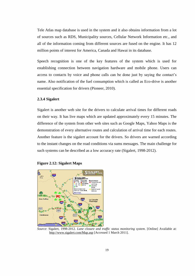
19
Tele Atlas map database is used in the system and it also obtains information from a lot
of sources such as RDS, Municipality sources, Cellular Network Information etc., and
all of the information coming from different sources are fused on the engine. It has 12
million points of interest for America, Canada and Hawai in its database.
Speech recognition is one of the key features of the system which is used for
establishing connection between navigation hardware and mobile phone. Users can
access to contacts by voice and phone calls can be done just by saying the contact’s
name. Also notification of the fuel consumption which is called as Eco-drive is another
essential specification for drivers (Pioneer, 2010).
2.3.4 Sigalert
Sigalert is another web site for the drivers to calculate arrival times for different roads
on their way. It has live maps which are updated approximately every 15 minutes. The
difference of the system from other web sites such as Google Maps, Yahoo Maps is the
demonstration of every alternative routes and calculation of arrival time for each routes.
Another feature is the sigalert account for the drivers. So drivers are warned according
to the instant changes on the road conditions via sums messages. The main challenge for
such systems can be described as a low accuracy rate (Sigalert, 1998-2012).
Figure 2.12: Sigalert Maps
Source: Sigalert, 1998-2012. Lane closure and traffic status monitoring system. [Online] Available at:
http://www.sigalert.com/Map.asp [Accessed 1 March 2011].

20
2.4 STATE-OF-THE-ART SOLUTIONS BY UNIVERSITIES
This section briefly describes the projects conducted by universities that aimed for
improving the traffic flow. Some of these projects are also supported by various
companies and/or government authorities.
2.4.1 Mobile Millennium
Mobile Millennium is a research project conducted by UC Berkeley, Nokia Research
Center, and NAVTEQ, with sponsorship from the California Department of
Transportation. Its main purpose has been to design, test and implement a system to
collect traffic data from GPS-equipped mobile phones and estimate traffic status in real-
time. It demonstrates a real-time permanent monitoring system capable of using GPS
data from thousands of vehicles in a metropolitan area to construct velocity fields and
travel time estimates. The system is able to monitor not only freeways, but also arterials
and secondary highways. The system is scalable, requires low bandwidth, protects the
privacy of its participants, and has the highest quality of information when compared
with existing traffic monitoring systems. During the development timeline, it conducted
a six month pilot deployment of GPS technology, where thousands of GPS mobile
phones were placed in vehicles within a focus area.
Figure 2.13: Mobile Millennium system architecture overview
Source: Work, D., Tossavainen, O.-P., Jacobson, Q. & Bayen, A., 2009. Lagrangian Sensing: Distributed
Traffic Estimation with Mobile Devices. In Proceedings of the 2009 American Control
Conference., 2009, pp. 1536-1543.
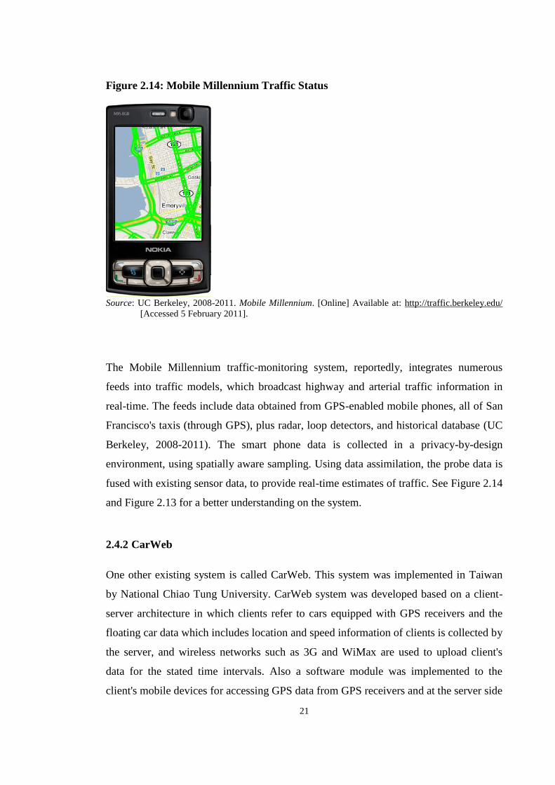
21
Figure 2.14: Mobile Millennium Traffic Status
Source: UC Berkeley, 2008-2011. Mobile Millennium. [Online] Available at: http://traffic.berkeley.edu/
[Accessed 5 February 2011].
The Mobile Millennium traffic-monitoring system, reportedly, integrates numerous
feeds into traffic models, which broadcast highway and arterial traffic information in
real-time. The feeds include data obtained from GPS-enabled mobile phones, all of San
Francisco's taxis (through GPS), plus radar, loop detectors, and historical database (UC
Berkeley, 2008-2011). The smart phone data is collected in a privacy-by-design
environment, using spatially aware sampling. Using data assimilation, the probe data is
fused with existing sensor data, to provide real-time estimates of traffic. See Figure 2.14
and Figure 2.13 for a better understanding on the system.
2.4.2 CarWeb
One other existing system is called CarWeb. This system was implemented in Taiwan
by National Chiao Tung University. CarWeb system was developed based on a client-
server architecture in which clients refer to cars equipped with GPS receivers and the
floating car data which includes location and speed information of clients is collected by
the server, and wireless networks such as 3G and WiMax are used to upload client's
data for the stated time intervals. Also a software module was implemented to the
client's mobile devices for accessing GPS data from GPS receivers and at the server side

22
of this system information was collected in the database and traffic status is estimated
for each road segment.
Figure 2.15: Architecture of CarWeb
Source: Chang, Y.-M. et al., 2009. Exploring GPS Data for Traffic Status Estimation. In Tenth
International Conference on Mobile Data Management: Systems, Services and Middleware.,
2009, pp. 369-370.
2.4.3 Performance Measurement System (PeMS)
A project to investigate various performance measures on the freeway system is called
Freeway Performance Measurement System (PeMS), conducted by University of
California, at Berkeley, with the cooperation of the California Department of
Transportation, California Partners for Advanced Transit and Highways, and Berkeley
Transportation Systems.
PeMS collects raw detector data in real-time, stores and processes this data, and reports
this data through a number of web pages such that engineers can analyze the
performance of freeway segments or of the overall freeway system. PeMS collects loop
detector data (over 25k individual detectors) from District 3, 4, 7, 8, 11, 12 and stores
them online. PeMS is also an Archived Data User Service (ADUS), contains 2 TB of
historical data (belongs to past 10 years) online, and adds 2 GB of data each day. The
data is available for research analysis.

23
Figure 2.16: PeMS real-time traffic conditions map
Source: PeMS, 2010. Performance Measurement System (PeMS) by Caltrans, UC Berkeley, and PATH.
[Online] Available at: https://pems.eecs.berkeley.edu [Accessed 2 May 2011].
Figure 2.17: PeMS System Overview
Source: PeMS, 2010. Performance Measurement System (PeMS) by Caltrans, UC Berkeley, and PATH.
[Online] Available at: https://pems.eecs.berkeley.edu [Accessed 2 May 2011].
PeMS is accessed via a standard Internet browser and contains a series of built-in
analytical capabilities to support a variety of uses. In order to use PeMS site, one must
apply for an account. The most important capabilities of the system are real-time traffic
estimation map, and travel time prediction on pre-defined routes. Prediction system is

24
based on the historical data. Moreover, the date range for the historical data can be
chosen by the users (PeMS, 2010).
2.4.4 DynaMIT
DynaMIT can be described as another solution for Advanced Traveler Information
Systems (ATIS) which is conducted by Massachusetts Institute of Technology (MIT).
The system is composed of two sub-systems: State Estimation and State Prediction.
Figure 2.18: DynaMIT state estimation and prediction processes using real-time
traffic data
Source: Antoniou, C.R., Balakrishna, H., Koutsopoulos, N. & Ben-Akiva, M.E., 2009. Off-line and online
calibration of dynamic traffic assignment systems. In Proc. 12th IFAC Symposium on Control in
Transportation Systems., 2009,
State estimation combines the available surveillance with historical information to
estimate the current state of the entire network. Pre-trip demand is simulated, allowing
drivers with different characteristics to dynamically change their departure time and
travel mode. This is followed by OD (Origin-Destination) flow estimation and network
estimation. The estimated network condition is then compared to surveillance
information. Inconsistent estimations are unaccepted and a new iteration of estimation is
initiated.
After the state estimation process, state prediction is done by first indicating the pre-trip
predictions then followed by OD (Origin-Destination) prediction and network state
prediction. DynaMIT system architecture is demonstrated in Figure 2.18.

25
2.4.5 *bus (Starbus)
Another research interest is developing a multi-functional box which can be used as a
part of bus arriving systems, which is developed by University of Washington. This box
can be implemented to the bus and passenger information system can be designed via
SMS. Box hardware consists of two components: GPS module for gathering location
information and GSM modem which can be combined in a single package using a local
SIM card. GSM modem is used for connecting central server via SMS messages.
Figure 2.19: Use of in-vehicle multi-functional box systems for receiving /
transmitting floating car data
Source: Anderson, R. et al., 2009. Building a transportation information system using only GPS and basic
SMS infrastructure. In International Conference on Information and Communication
Technologies and Development (ICTD)., 2009, pp. 233-242.
Central server updates and stores GPS data for indicated time intervals and the
components of the server can be declared as: a laptop computer which is connected to
GPS-enabled mobile phone and serves as an SMS gateway. Server uses MySMS which
is an application framework for implementing a system that connects via SMS.

26
Table 2.2: Comparison of existing traffic solutions I
Source: Türk Telekom Technical Report, 2011; Robust Traffic Status Estimation and Adaptive Traffic
______ Signaling, December 2011.
Name /
Partner
Subcategor
y
Requireme
nts
Provide
rs Approach Challenges
Predic
tion
Real-
Time
Data
MSNDirect
USA
2004-2010
Location Based
Services
MSNDirect is widely used
with GPS
devices. Each company
should design
their own software for
implementing
the system
Microsoft
The system provides real-
time traffic information by
Microsoft Directband channel
Microsoft DirectBand can
be used only with
one FM channel and additional
hardware is
required. Also data feeds are
required for the
system
TomTom
HD Traffic
Netherlands
- Portugal
Advanced Traveler
Information
System (ATIS)
Navigation
Device
TomTom
navigation
device has to be
implemented to
the car for using the
system which is
widely called as TomTom HD
Traffic
Vodafone -
TomTom
TomTom has a data fusion engine for estimating the
current status of traffic.
The engine takes 5 inputs from different sources to
provide more accurate
information.Vodafone’s GSM probe data is the one
of this sources which is
taken by calculating the traffic status by counting
the mobile phones along
the route and displays alternative routes
according to the
TomTom's IQ technology.
Providing real-
time information
from GSM Probe Data has many
challenges : such
as identifying the irrelevant probes,
decide the
direction and speed of the
vehicle and
identifying whether the
signals are
coming from the same vehicle or
not
CarWeb
Taiwan
2008-2010 Chiao Tung
University
Advanced Traveler
Information
System (ATIS)
GPS Data Logger
3G Smart
Phone
Web Server
Database
Server
Chiao
Tung University
System collects real-time
data from GPS Probes via 3G and WiMax
Challenges can be divided into two
subcategories as
network challenges of 3G
and WiMAX and
the accuracy of using single data
source such as
GPS.
IBB Traffic
Turkey
2009-2010
Advanced
Traveler
Information System (ATIS)
No additional
hardware is
required.
IBB-
Microsoft
IBB Traffic is the mobile application that uses
cameras, sensors and real-
time information data
which is provided by IBB,
as the sources. Image
processing is used for estimating the current
status of traffic
System mainly
uses cameras for
the estimation but
traffic cameras
are located

27
Table 2.3: Comparison of existing traffic solutions II
Source: Türk Telekom Technical Report, 2011; Robust Traffic Status Estimation and Adaptive Traffic
______ Signaling, December 2011.
Name Subcategory Requirem
ents Providers Approach Challenges
Predicti
on
Real-
Time
Data
Smart Bus
Stop
Turkey
2009-2010 / Istanbul
Technical
University
Road Side Unit –
ATIS(Advanced
Traveler Information
System)
Sensors for
buses, and
screens for the stations
are required
IBB –
ISBAK
Smart Bus Stop can be
categorized as a road
site unit which is stated at every bus
stations and provides
real-time bus information such as
arrival time of the bus,
current traffic status,
current location of the
bus etc.
Network
challenges on
road side units such as
broadband
limitations are main challenges
of the system
RDS Link
China
2008-2010 /
Rice
University
ATIS(Advanced
Traveler
Information System)
FM Receiver
Motorola
Qualcomm
Inc.
RDS Link is a system which provides an
interface to implement
RDS-TMC channel sources to the existing
software
The main challenges of
using RDS-TMC
channel as a real-time information
provider are the
broadband challenges and
the
implementation of RDS to the
existing software
DynaMIT
USA
2009-2010 / MIT
ATIS(Advanced
Traveler
Information Systems)
GPS enabled
cell phones
Massachusetts Institute of
Technology
DynaMIT collects
real-time traffic data
from GPS Probes, and
evaluation of the information is done on
the simulation layer of
the system and MITSIM is used as a
simulation tool
Complexity of
the algorithms
causes a low-speed system
Short
Term
Prediction
Mobile
Millennium
USA
2008-2010 /
UC
Berkeley
ATIS(Advanced
Traveler Information
System)
GPS enabled cell phones
Nokia – UC Berkeley
System architecture is
based on using GPS enabled cell phones to
provide real-time
information and demonstrating the
estimation of the
current traffic status on
live maps in a mobile
application
Mobile
Millennium uses GPS probe data
for estimation
and usage of one kind of data as a
source decreases
the accuracy of the system
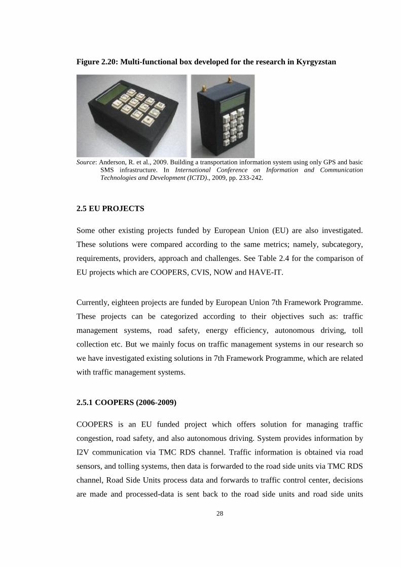
28
Figure 2.20: Multi-functional box developed for the research in Kyrgyzstan
Source: Anderson, R. et al., 2009. Building a transportation information system using only GPS and basic
SMS infrastructure. In International Conference on Information and Communication
Technologies and Development (ICTD)., 2009, pp. 233-242.
2.5 EU PROJECTS
Some other existing projects funded by European Union (EU) are also investigated.
These solutions were compared according to the same metrics; namely, subcategory,
requirements, providers, approach and challenges. See Table 2.4 for the comparison of
EU projects which are COOPERS, CVIS, NOW and HAVE-IT.
Currently, eighteen projects are funded by European Union 7th Framework Programme.
These projects can be categorized according to their objectives such as: traffic
management systems, road safety, energy efficiency, autonomous driving, toll
collection etc. But we mainly focus on traffic management systems in our research so
we have investigated existing solutions in 7th Framework Programme, which are related
with traffic management systems.
2.5.1 COOPERS (2006-2009)
COOPERS is an EU funded project which offers solution for managing traffic
congestion, road safety, and also autonomous driving. System provides information by
I2V communication via TMC RDS channel. Traffic information is obtained via road
sensors, and tolling systems, then data is forwarded to the road side units via TMC RDS
channel, Road Side Units process data and forwards to traffic control center, decisions
are made and processed-data is sent back to the road side units and road side units

29
forward data to the Human Machine Interface System in cars to display safety warnings
and alternative routes.
Figure 2.21: System architecture of COOPERS solution
Source: COOPERS, 2006-2010. European Union ITS Project: COOPERS. [Online] Available at:
http://www.cooper-eu.org [Accessed 13 October 2010].
2.5.2 NOW (2008-2009)
Another project which is funded by EU is “Network on Wheels” (NOW). The objective
of this project is to provide car-to-car and car-to-infrastructure communications for
traffic management. System mainly has 3 elements: On-board Units (OBU), Application
Units (AU) which are in cars on roads and Road Side Units (RSU) on roads. Two
different technologies are used for establishing the connection between OBU’s and
RSU’s and these are: GPS and Wireless LAN IEEE 802.11. Two different OBU's are
communicated via ad hoc networks and OBU's and RSU's are communicated using
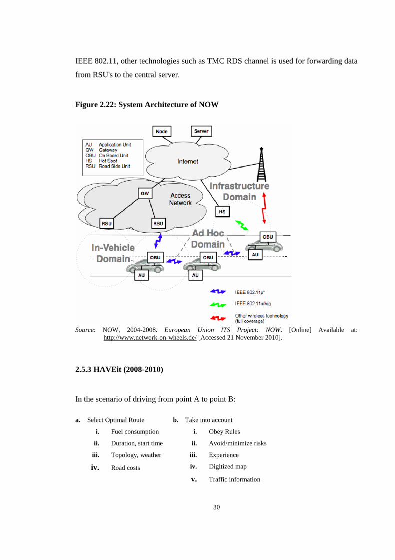
30
IEEE 802.11, other technologies such as TMC RDS channel is used for forwarding data
from RSU's to the central server.
Figure 2.22: System Architecture of NOW
Source: NOW, 2004-2008. European Union ITS Project: NOW. [Online] Available at:
http://www.network-on-wheels.de/ [Accessed 21 November 2010].
2.5.3 HAVEit (2008-2010)
In the scenario of driving from point A to point B:
a. Select Optimal Route
i. Fuel consumption
ii. Duration, start time
iii. Topology, weather
iv. Road costs
b. Take into account
i. Obey Rules
ii. Avoid/minimize risks
iii. Experience
iv. Digitized map
v. Traffic information

31
HAVEit is an EU-funded project, and it provides a scalable vehicle architecture, by
means of smart sensors, standard fail silent Electronic Control Units (ECU) and smart
actuators, will be defined to cope with the needs for highly automated driving, based on
conventional actuators up to fail tolerant integration of drive-by-wire to allow
autonomous driving (HAVEit, 2008-2011). Various sensors in cars are used for traffic
management applications, and human machine interface is designed for driving
assistance system.
Figure 2.23: HAVEit - Decision Mechanism & Optimum path from source A to
destination B
Source: HAVEit, 2008-2011. European Union ITS Project: HAVEit. [Online] Available at:
http://www.haveit-eu.org [Accessed 20 December 2010].
2.5.4 CVIS (2007-2010)
CVIS is the another existing solution which is funded by EU, and its objectives include
providing real-time information to the drivers, establishing car-to-car and car-to-
infrastructure communications, providing parking slot management and developing
adaptive traffic light system and VMS (Vehicle Message System). CVIS collects
floating car data via GPS and broadcasts this data using TMC RDS channel.

32
Table 2.4: Comparison of European Union projects and solutions
Name &
Period
Subcategory Requirements Providers Approach Challenges
COOPERS
(2006-
2010)
Vehicle to
vehicle and
vehicle to
Infrastructure
communication
The
implementation of
this project
requires road side
units.
European Car-to-
Car
Consortium.(Aust
ria Tech)
Supported by EU
6th Framework
Programme
This project
focuses on the
advance of
telematics
applications on
the road.
The system
requires in-
vehicle units,
road side units.
Lots of
hardware
implementation
is required.
CVIS
(2006-
2010)
Advanced
Traveler
Information
System (ATIS)
V-2-V and
V-2-I
communication
System provides
communication
between cars and
infrastructure by
especially using
“Wi-Fi for
mobiles”. It also
uses 3G and
DSRC for
communication
European Car to
Car Consortium
(EU funded
project)
To create a
technical
solution
allowing all
vehicles and
infrastructure
elements to
communicate
with each other
in a continuous
and transparent
way using a
variety of media
and with
enhanced
localization
The network
limitations of
Wi-Fi and 3G.
Also network
violence can be
explained as
another
challenge.
NOW
(Network
on Wheels)
(2008-
2012)
Car-to-Car
Communication
On-board Units
are required
European Car to
Car Consortium
EU Funded
Project
System collects
data via ad hoc
networks and
IEEE 802.11
Specification of
position based
routing and
forwarding
protocols,
adaption of
wireless LAN
under realistic
radio conditions
HAVE-IT
(2008-
2012)
Advanced
Traveler
Information
System (ATIS)
ADAS joint
system
On-board Units
are required
European Car to
Car Consortium
EU Funded
Project
Design of the
task repartition
between the
driver and co-
driving system
(ADAS) in the
joint system
Designing of
HMI's (Human
Machine
Interface) and
complexity of
DSU algorithm
Source: Türk Telekom Technical Report, 2011; Robust Traffic Status Estimation and Adaptive Traffic
______ Signaling, December 2011.

33
Figure 2.24: CVIS system architecture
Source: CVIS, 2004-2010. European Union ITS Project: CVIS. [Online] Available at:
http://www.cvisproject.org/ [Accessed 17 October 2010].
The system provides car-to-car communication (DSRC), hot-spots (wireless LAN) and
also WiMAX communications. Park Slot Management is one of the key features of this
project and the data related to parking is obtained using DSRC connection.
2.6 COMMUNICATION TECHNOLOGIES
This section briefly explains the possible communication services that can be used in
the smart transportation systems. Communication technologies which are used in many
ITS researches, can be subcategorized into two parts: Traditional Communication
Technologies and the Vehicular Communication Technologies. Each of these
technologies that have advantages on their own is provided below.
2.6.1 Traditional Communication technologies
Traditional Communication technologies can be divided into two subcategories as
Infrastructure based and infrastructure-less according to their communication ranges.
Infrastructure based technologies have a long communication range while
infrastructure-less technologies have less than 1km communication range. These
technologies can be listed as Cellular Communications (GPRS, 3G, LTE, EVDO),

34
WiMAX, DVB, WLAN, Infrared, Bluetooth, ZigBee, Millimeter-wave (MMWAVE)
(Dar et al., 2010), (Huang & Chen, 2009).
Figure 2.25: A classification of Wireless Communication Technologies used in ITS
Source: Dar, K. et al., 2010. Wireless communication technologies for ITS applications [Topics in
Automotive Networking]. IEEE Communications Magazine, 48 (5), pp.156-162.
2.6.2 Vehicular Communication Technologies
Since ITS market improves, the need for special communication technologies increases.
Vehicular communication specific networks were developed to satisfy the increased
sensor based applications requirements. These are basically, DSRC (Dedicated Short
Range Communication), WAVE (Wireless Access in the Vehicular Environment),
CALM (Communication Air interface for Long and Medium range) (Huang & Chen,
2009).

35
Table 2.5: Comparison of wireless communication technologies for Smart
Transportation Systems
Data
Rate Range Mobility
Operating
Band Latency Usage Area in ITS
GSM/GPRS 80-384
Kb/s 10km Yes
0.8-1.9
GHz
1.5-3.5
sec
Incident Management
Traffic Management
Infotaintment
WiMAX 1-32
Mb/s 15km Yes 5.x GHz 110 ms Contextual
Applications
DVB/DAB 1.73
Mb/s 40km Yes 6-8 MHz 10-30 sec
Traffic Management
Contextual
Applications
WLANs(a/b/
g/n)
54-600
Mb/s 250m Limited
2.4-5.2
GHz 46 ms In Vehicle
Connection
MMWAVE 1 Gb/s 10m Limited 60-64 GHz 150 µs In Vehicle
Connection
IR 1 Mb/s 10m No 2.6 GHz Very
Low Road Monitoring
ZigBee 20-250
Kb/s 100m Yes
2.4-2.5
GHz 16 ms Road Monitoring
Bluetooth 1-3 Mb/s 10 m Limited 2.4 GHz 100 ms On Board
Applications
DSRC/WAV
E
6-27
Mb/s 1 km Yes
5.8-5.9
GHz 200 µs
Collision Avoidance
Road Sign
Notifications
Incident Management
Traffic Management
Contextual
Applications
Road Monitoring
CALM (M5) 6 Mb/s 1 km Yes 5-6 GHz 200 µs Road Sign
Notifications
Source: Türk Telekom Technical Report, 2011; Robust Traffic Status Estimation and Adaptive Traffic
______ Signaling, December 2011.

36
3. ROBUST TRAFFIC STATUS ESTIMATION
It is often mentioned as a solution that can tackle the congestion is to construct new
roads as well as enlarge current motorways in order to increase the capacity of the
infrastructure (Bellemans et al., 2003). However it is a costly work and a long-term
solution. What these cities require is a cost-effective and short-term solution.
Knowing the shortest route to the destination does not solve any problems in today’s
crowded cities. It only serves as the basic approach for supplying information such as
travel length and travel time under free flow which is calculated with the speed limits of
the corresponding roadway. Even knowing the real-time travel information cannot help
the travelers since the traffic states are extremely unstable. None of the travelers that
check the real-time traffic congestion can know what kind of surprises await them
during a trip. What people need to and want to know are the answers to the questions
like: “What is going to happen after 10 minutes?”, “Will the traffic that is occurring 10
km ahead affect my trip?”, “How long it will take for me to go to home if I leave the
office 15 min later from now?” Because the unstable characteristics of the road traffic
may lead to traffic states which are quite the opposite of what we see on and expect
from the real-time traffic screens.
The role of traffic models in this sense is beyond the foreseen. They play quite an
important part in both contemporary traffic research and traffic applications such as
traffic control, incident detection and flow prediction. The biggest impact of the traffic
models come from the fact that it provides the only possible way that can help not just
to interpret the effects of the traffic congestion, but also to build up a mechanism to
predict the near future congestion states of the system which are commonly up to 30
minutes. Predicting the future congestion states enables the users to optimize their
departure time in advance, hence providing them an effective time management
possibility. It serves as a short-term approach to solve, reduce or at least postpone the
traffic problem.

37
3.1 TRAFFIC THEORY EQUATIONS AND BASICS
The most common equation used in the traffic theory is the one that introduces the
relationship between Flow (q), Density (ρ) and Velocity (v):
, Flow = Density . Velocity (3.1)
Density can also be expressed as the reverse of spacing between the vehicles. That is.
, Density = 1 / Spacing (3.2)
3.2 TRAFFIC THEORY PARAMETERS
Traffic theory is a hard to handle and explain phenomenon without the help of some
specific set of parameters. The most common terms used in equations and discussions
are explained in this section.
i. : is the parameter that is also known as flow variable. Flow is determined
as the number of vehicles that pass from a fixed point per hour and is given in
terms of vehicles per hour (veh/h). It is the most common parameter in traffic
theory. A 10 min volume can be converted to flow by multiplying its value with
6, since 10 min is the one sixth of an hour. For instance, if a 10 min volume of a
road segment is 100 vehicles then its equivalent rate in terms of flow is 600
veh/h.
ii. : is the parameter that is also known as density variable. Density is
determined as the number of vehicles present on a given length of roadway, and
is reported in vehicles per km (veh/km) or mile at a particular time instant.
Higher densities imply that the vehicles are quite close to each other while low
densities indicate long distances (spacing) between vehicles.

38
iii. : stands for the speed (velocity) of a vehicle at a given time instant. It is
defined as the distance traveled within a certain amount of time, e.g. km/h. Since
the speed of vehicles will differ from each other, the average speed should be
taken into account in traffic flow calculations. In our calculations we take the
average speed of many vehicles inside a road segment.
Figure 3.1: Basic parameters of Traffic Flow shown on a three segment roadway
Source: Türk Telekom Technical Report, 2011; Robust Traffic Status Estimation and Adaptive Traffic
______ Signaling, December 2011.
iv. : The arithmetic mean of the speed of those vehicles
occupying a given length of road at a given instant. It is calculated as
∑ )
v. : The arithmetic mean of the speed of vehicles passing a
point during a given time interval. It is calculated as (
)∑

39
vi. : This is the vehicle length which is used to calculate both jam density
and critical density . We take it as approximately 5.5 meters in our
calculations.
vii. : Spacing is the physical distance (space) between two vehicles and is the
inverse of density. The space referred here is measured between the front
bumper of the leading vehicle and the front bumper of the following vehicle.
Space is the product of speed and headway and generally given in unit of meters.
viii. : Clearance is similar to spacing. However, clearance indicates the
distance between the rear bumper of the leading vehicle and the front bumper of
the following vehicle. In this sense, clearance equals the spacing minus the
length of the leading vehicle. Again similar to spacing, its unit is in meters.
ix. : Headway stands for the temporal space between two consecutive
vehicles. To get into more detail, it is the time which elapses during the arrival
of leading vehicle and the following vehicle at a fixed point. Headway variable
is generally determined as in seconds.
x. : Gap is a similar to headway parameter. It is the measure of time that
elapses during the departure of the first vehicle and arrival of second vehicle at a
given point. It is measured between the rear bumper of the lead vehicle and the
front bumper of the second vehicle, where headway refers to front to front
bumper times. Unit of gap is in seconds.
xi. : It is the number of vehicles that pass a given point on the
roadway in a specific period of time. For instance, a 10 minute volume means
the counted number of vehicles that passed the fixed point on the roadway

40
during a 10 minute period. Usually, volume is directly converted to flow (q) for
convenient calculations.
xii. : This describes the relationship between hourly volume
and the maximum rate of flow within the hour: PHF = hourly volume/maximum
rate of flow. For the 15 minute periods, PHF = volume/4 x (maximum 15 minute
volume within the hour). PHF = q60/q15 (Wei et al., 2009).
xiii. : Shockwaves occur as a result of differences in flow and density
which occur when there are constrictions in traffic flow. These constrictions are
called bottlenecks. The speed of growth of the ensuing queue is the shockwave,
and is the difference in flow divided by the difference in density. For instance,
when a crash occurs and one or more of the lanes are closed to traffic a
bottleneck occurs right at that crash zone. This bottleneck will cause a
shockwave traffic along the crash zone.
Figure 3.2: Shockwave analysis on a time-space diagram
Source: Türk Telekom Technical Report, 2011; Robust Traffic Status Estimation and Adaptive Traffic
______ Signaling, December 2011.

41
xiv. : It occurs when the flow is periodically interrupted by the
external entities, primarily by the traffic control devices.
xv. : It occurs when vehicles traveling on a route are
not affected by external conditions such as traffic signaling devices that might
possibly interrupt their normal cruise.
xvi. : The total time spent between when vehicle starts traveling from
source point and reaches to destination point over a specified route under regular
conditions.
3.3 FUNDAMENTAL DIAGRAM
Fundamental diagram is used to show the basic relationship between the flow
(vehicle/h) and density (vehicle/km) at a given location or section of the motorway. In
other words, it describes the behavior of traffic in aggregated variables (average speed,
average density, and average flow). Fundamental diagram is one of the basic concepts
in traffic theory because of the comprehensive insight it provides. In addition, the
determination of the traffic dynamics such as maximum traffic flow (Qmax, a.k.a.
capacity, measured in vehicle per hour), critical density ( , measured in vehicle per
km), jam density ( , measured in vehicle per km), free flow speed (
, measured in km
per hour) and congestion wave speed (w, measured in km per hour) for a particular
segment of a roadway are found by the fundamental diagram.
The relationship between density and velocity can be explained as the more vehicles on
the road, the slower the velocity. Fundamental diagram can play the role of a controller
where the vehicles entering a road should be equal to vehicles leaving the road. Hence
the traffic flow can be kept stable. State of the flow changes to unstable when a critical
density is reached.

42
3.4 TYPES OF THE FUNDAMENTAL DIAGRAM
There are three types of Fundamental Diagram in traffic systems. These can be listed as:
a. Flow-Density
b. Speed-Density
c. Speed-Flow
The one most related to our research is the flow-density diagram. Flow density diagram
is used to give the traffic conditions of a roadway. With the help of pre-determined
traffic conditions, time-space diagrams can be created to give travel time, delay, and
queue lengths of a road segment.
If we observe the traffic for a segment over the roadway and plot the flow (veh/h)
versus the density (veh/km/lane) for the related segment a curve similar to that in Figure
3.3 occurs. This curve has a characteristic shape which is the same for every roadway
section.
Figure 3.3: Flow-Density Fundamental Diagram in traffic theory
Source: Türk Telekom Technical Report, 2011; Robust Traffic Status Estimation and Adaptive Traffic
______ Signaling, December 2011.

43
When the density is zero which means there are no vehicles in the road, then flow is
definitely zero, as well. Traffic flow increases with increasing traffic density. Increasing
the traffic density more will result a slowing down effect on the increment rate of traffic
flow. After a specific point, the flow reaches a maximum for a density that in the
literature called the critical density ( . When the density is greater than the critical
density, the traffic flow on the roadway starts decreasing. As the density increases
further, the flow converges to zero for a density that is called the jam density ( in the
literature.
There are two types of flow-density graphs. One of them is the triangular shaped flow-
density curve, which is in the context of our research and also viewed as the more
realistic one by the academia. The other one is the parabolic shaped flow-density curve.
The triangular shaped fundamental diagram consists of two vectors. The first one
represents the free flow (Vf). It starts from the origin and goes up until the capacity point
designated by Qmax and calculated via the slope of the corresponding vector. The other
vector represents the congested situation of the road. It is named as congestion wave
speed vector which is placed between Qmax and the point representing the zero flow and
jam density ρj. At the congested part of the diagram, there is a negative slope which
introduces the fact that the higher the density the lower the flow. Intersection of these
two vectors is the maximum possible flow that can be achieved under free flow speed.
3.5 PARAMETERS OF THE FUNDAMENTAL DIAGRAM
Parameters that appear on the Flow-Density fundamental diagram are explained in this
sub-section. Each of these parameters is essential for obtaining the fundamental
diagram, and hence a realistic road network configuration. Obtaining the right diagram
lets us to get better real-time simulation and prediction results because of the realistic
input.
i. : Free flow speed, meaning in the speed in an uncongested section.
Most of the time equals to the speed limit in the corresponding section.

44
ii. : Congestion wave speed, meaning in the speed that the traffic starts to
slow down after reaching the maximum flow on the road section. Most of
the time, it is seen along the bottlenecks where the shockwaves occur.
iii. : Maximum flow (capacity), meaning in the traffic condition at which the
maximum # of vehicles can pass by a point within a given time period.
iv. : Critical density stands for the threshold that the change in density does
not affect the free flow speed. It is the maximum density achievable under free
flow.
v. : Jam density stands for the minimum density achievable under
congestion.
3.6 CALIBRATION OF THE FUNDAMENTAL DIAGRAM
There are two equations corresponding to the relations between maximum flow Qmax,
critical density , jam density
, free flow speed and congestion wave speed w.
,
(3.3)
,
(3.4)
However, there are more than one unknown parameter. We calculate some of the
unknown parameters with the equations below:
(3.5)
45
(
) ⁄ (3.6)
We assume the free flow on freeways equals the pre-determined value by the
“Karayolları Genel Müdürlüğü”, which is implemented as 120 km/h. Another known
parameter is the section length which is determined during the segmentation process of
the freeway. We take the vehicle length as approximately 5.5 m.
Section Length / Vehicle length stands for the Jam Density ( ) and is the seven times
of Critical Density ( ) in the traffic theory.
3.7 MATHEMATICAL TRAFFIC FLOW MODELS
There exists a wide variety of traffic models. The models are classified based on their
specific attributes. There are four different factors used in the classification process, 1)
Physical interpretation, 2) Level of detail, 3) Discrete versus continuous, 4)
Deterministic versus stochastic.
Physical interpretation consists of three major approaches, namely white box, black box,
and grey box. In black box modeling, input and output data are recorded and a generic
parameterized model is fitted to the data. In white box modeling, physical equations
describe the relationships between the different states of the traffic system. In the
middle of these models, an intermediate model is the grey box modeling, which is the
combination of the other two, and comprised of two phases. In the white box phase,
parameterized equations of the motorway states are described; whereas in the black box
phase, input/output relation of the traffic model are fitted to input/output measurements,
thus the parameters are calibrated. LWR model (Richards, 1956), (Lighthill & G.B.,
1955) and Payne model (Payne, 1979), (Payne, 1971) are the products of such a method.

46
Figure 3.4: Classification of the Traffic Flow Models
Source: Türk Telekom Technical Report, 2011; Robust Traffic Status Estimation and Adaptive Traffic
______ Signaling, December 2011.
Another way of classifying the traffic models is to determine whether it is a
deterministic or a stochastic approach. Deterministic models provide a deterministic
relation between the states of the system, as well as the inputs and outputs of the related
system. In a deterministic approach, simulating a traffic situation more than once with
not only the same initial and boundary conditions but also the same input parameters,
the results of the simulation will exactly be the same. For instance, the macroscopic
model developed by Payne is a deterministic model. On the other hand, stochastic
traffic models contain one or more stochastic variable(s). Having at least one stochastic
variable means that the results of the two separate simulations of the same model run
with the same initial and boundary conditions and the same inputs might yield different
results which is directly affected by the stochastic variable’s value in each simulation.
Paramics simulation tool is an example of such a model. The tool is a microscopic
model that requires the distribution function of the level of patience over different
drivers to be defined. In every new simulation, this parameter is found by a new
sampling of the distribution. Considering large traffic networks, stochastic models have
Classification Factors
Physical Interpretation
White Box
Black Box
Grey Box
Level of Detail Macroscopic
Microscopic
Continuity Continuous
Discrete
Based on Processes Deterministic
Stochastic

47
a major drawback in terms of computational power requirements. This project aims at
an online prediction mechanism which increases the impact of the computational
requirement which makes the stochastic models even more undesirable.
All of the traffic flow models are based on describing the evolution of variables on the
corresponding roadway – also known as state variables – over time. Obviously, it
consists of two independent variables, namely, time and space. These independent
variables can be considered to be either discrete or continuous. For example, the Payne
model is continuous in nature. However, the continuous models are too complex that for
proper calculation they are discretized. It would not be possible to solve them in real-
time if the size of the road network is huge. Payne model is also discretized in both time
and space (15 seconds and 500 meters in common) to be able to be simulated by a
computer.
The most known model classification is done according to level of detail. Level of
detail based classification is composed of two types of traffic flow approaches, one of
which is in macroscopic level; the other is in microscopic level. The microscopic flow
approach resulted in car-following theory which studies the interactions of one vehicle
following the other. On the other hand, macroscopic approach studied the similar
behaviors of the fluid dynamics or continuum theories. Unlike microscopic models that
studies the individual vehicle dynamics, macroscopic models lack a big level of detail,
however gain the ability of monitoring and dealing with the issues of a large scope.
What is making a significant difference in macroscopic models is the conservation law
of vehicles just like in the fluid mechanics. Conservation law is quite useful especially
in describing the waves in a traffic stream, vehicles passing through the waves, and their
speed (Haefner & Li, 1998).
3.7.1 Microscopic
Microscopic simulators refer to simulations of all vehicles or particles of the system that
are individually identified. Each vehicle’s position and velocity define the state of the
systems as dependent variables of time. The systems are mathematically represented
with ordinary differential equations. The models defined for every single vehicle are the
interactions between the vehicles or between the vehicles and the terrain (roadway). In

48
such a system, all the vehicles and their interactions with the environment are calculated
and in the end the whole system is shown as a snapshot.
Figure 3.5: Microscopic Model Simulation
Source: Paramics, n.d. Paramics Traffic Simulator. [Online] Available at: http://www.paramics-
online.com/ [Accessed 23 July 2011].
In Microscopic models the roadway setup is described in terms of fundamental
parameters such as overtaking rules, speed limits, number of lanes, etc. In addition to
the environmental setup, the vehicles are described one by one in terms of individual
parameters such as driver’s patience, aggressiveness, reaction time, acceleration,
deceleration behaviors; the vehicle’s origin, type (bus, minibus, van, etc.) , destination,
etc. Both the driver parameters and the vehicle parameters are sampled from a
predefined stochastic function that is supposed to be based on the measurements of real
life traffic. Each vehicle tries to reach its destination according to the model defined
individually for its own. During the whole trip starting from the origin, they interact

49
with each other by overtaking moves and interact with the environment such as obeying
the speed limits according to their own microscopic vehicle models.
Figure 3.6: Individually defined vehicles in a system that form the concept of
Microscopic Traffic Models and Simulation
Source: Paramics, n.d. Paramics Traffic Simulator. [Online] Available at: http://www.paramics-
online.com/ [Accessed 23 July 2011].
Microscopic traffic flow models are able to yield more accurate and detailed
representation of a traffic system, however they require intensive computational power
which makes them typically not suitable for real-time implementations. Nonetheless,
such implementations are vital for the development of advanced transportation solutions
(Zhang et al., 2000) since they help to analyze very small changes in the traffic stream
over time and space.
The most known microscopic models are 1) the car following model, 2) the overtaking
model.

50
3.7.1.1 Car following model
Car following model (Kesting & Reiber, 2008) tries to determine how the vehicles tend
to follow one another. The model describes the headway (distance) a driver preserves
between the own vehicle and the preceding vehicle, in addition to how the driver reacts
on traffic in front of its own, in other words the reaction to the acceleration and
deceleration of the preceding vehicle. There are two types of parameters defined for the
model. The first type introduces vehicle related parameters such as aggressiveness of
the driver, size (mass) of the vehicle, acceleration and deceleration. Second type
introduces the roadway-setup specific parameters such as speed limit, number of lanes
affecting the way a vehicle follows the one in its front.
Figure 3.7: Notation for Car Following Model
Source: Mathew, T.V., n.d. Microscopic Traffic Flow Modeling. [Online] Department of Civil
Engineering, Indian Institute of Technology Bombay Available at:
http://www.civil.iitb.ac.in/tvm/1100_LnTse/509_lnTse/plain/plain.html [Accessed 10
November 2011].
3.7.1.2 Overtaking model
Overtaking model studies the way a driver decides whether or not to overtake the
vehicle in the front. In this microscopic model the key attributes are the driver’s desired
speed and the vehicle’s acceleration capabilities. Besides, vehicle’s interactions with
other vehicles and the number of lanes on the road are the other properties that have
influence on the overtaking model. Subject vehicle’s driver decides to overtake
depending not only on the speed difference of the own lane and the lane adjacent to it,
but also on the available gap on the adjacent lane that determines whether or not it is
possible.

51
3.7.2 Macroscopic
Unlike microscopic models that represent individual vehicle interactions, macroscopic
models have the ability to deal with problems related to a larger scope by sacrificing a
decent deal of detail. Macroscopic traffic flow approaches follow the fundamentals
similar to that of fluid dynamics or continuum theories. Macroscopic traffic models are
often derived using the analogy between traffic flows and fluid flows where the
movements of the vehicles exhibit the attributes of the fluid motion (Javed et al., 2010).
The most prominent feature of the macroscopic models is the conservation law of
vehicles which states that the number of vehicles entering the traffic system must be
equal to the vehicles leaving the system.
Macroscopic traffic flow models are characterized in terms of the aggregate variables
such as traffic density, space mean speed and traffic flow. Aggregate traffic variable
stands for a variable that summarizes information about multiple vehicles. For example,
average speed is comprised of the speed of all vehicles present in a given section of the
road (Bellemans et al., 2003). In other words, the state of the traffic system is described
by the averaged gross quantities regarded as dependent variables of both time and space.
The traffic flow is defined as the number of vehicles passing a fixed point per hour and
the traffic density is defined as the number of vehicles per kilometer and per lane. Being
the functions of two dimensional space (x,y) and time (t) is one of the prominent
features of Macroscopic traffic models. Moreover, dynamics of the macroscopic models
are described using partial differential equations.
A classification based on the order of the models can be made within the class of
macroscopic models. The first macroscopic model developed is LWR (Lighthill-
Whitham-Richards) and is a first-order model. The model described by Payne (Payne,
1979), (Payne, 1971) is a second order model since it has two different state variables,
namely density and average velocity. Another higher order model is developed by
Papageorgiou (Papageorgiou et al., 1990). These three models are the most used ones in
practice. Although we have investigated these approaches thoroughly, our project is
based on another macroscopic model called CTM (Cell Transmission Model) which is
going to be discussed in detail later on. But note that the CTM is also based on the same

52
density calculation approach. Thus it can be said that the CTM is not far cry from these
models.
Figure 3.8: Aggregated variables and vehicle clusters that form the basis of
Macroscopic Traffic Models and Simulation
Source: Türk Telekom Technical Report, 2011; Robust Traffic Status Estimation and Adaptive Traffic
______ Signaling, December 2011.
Macroscopic models require less computational power compared to microscopic models
since they do not describe the traffic situation on the level of independent variables like
microscopic models do. Thus it is possible to quickly simulate a with the macroscopic
traffic flow models which is a compulsory requirement for online prediction
mechanisms. The fact that the macroscopic models have fewer parameters to estimate
allows easier calibration and identification of such models. Hence they are better suited
for optimal predictive mechanisms.
Furthermore in this section, we will give some insight on three macroscopic models,
namely, LWR, Payne and Papageorgiou.

53
3.7.2.1 LWR model (Lighthill – Whitham – Richards) (first order)
Macroscopic models mimic the analogy between the fluid flows and traffic flows. There
exists a law of conservation of vehicles similar to the law of conservation of mass in
fluid dynamics literature.
The first macroscopic model is developed by Lighthill and Witham (1955) and later
modified by Richards (1956) and its current form was developed. In LWR model there
exist only one state variable (density) that resulted in poor momentary behavior. Payne
later on (1971) coped with the problem by introducing another partial differential
equation that represents the dynamics of the mean speed onto the existing LWR model
(Javed et al., 2010), (Bellemans et al., 2003), (Haefner & Li, 1998), (Papageorgiou et
al., 1990), (Payne, 1979), (Payne, 1971).
Conservation of vehicles in traffic context can be represented as
(3.7)
where is the number of lanes at position x, denotes the traffic density in
vehicle/lane/km at location x and time t, stands for the traffic flow in
vehicle/hour at location x and time t. Among the aggregated variables both and
are the continuous functions of time and space. However the system is actually
not continuous, in the contrary, it is a discrete system since the vehicles on the roadway
are discrete. The equation of conservation states that none of the cars can appear
suddenly out of blue nor they can vanish, which complies with the law of physics.
The analytical solution as well as the implementation on the computer of the partial
differential equations is extremely hard. In order to cope with both complications a
discretization process is needed. Discretizing the differential equation for flow yields
the fundamental equation that describes the flow in terms of density and velocity. The
equation tells that the average flow in each section is average velocity times the traffic
density times the number of lanes of that section:

54
(3.8)
LWR model observed that the average velocity of vehicles can be expressed as a
function of traffic density.
( ) (3.9)
There is several velocity calculations expressed as a function of density. The idea
behind these equations tries to represent the relationship of velocity and density such
that the average velocity will drop until zero when the roadway becomes congested.
One of the empirical velocity formulas is:
( ) [ (
)
]
(3.10)
where stands for the free flow speed expressed as the average velocity of all the
vehicles belong to section , is the average speed in equilibrium, is the jam
density which where the average velocity is zero, and are parameters to be
calibrated. Parameters that require calibration are needed to be fitted on the traffic data
(Bellemans et al., 2003).
LWR is a continuum flow model in both time and space. In order to practically solve
this continuum model in a computer simulation the equations are discretized in both
time and space which is illustrated in Figure 3.1. Discretization of time is represented
with (in our case 10 second intervals). The discretization of space is done in terms of
kilometers and represented by either or (length of section usually in 0.5km to
1km where the main requirement is defined as . In other words, the minimum
space discretized should be greater than the space that can be traveled within one time
step under free flow speed condition.
The difference equation represents the LWR model is found by discretizing the
conservation Equation (7) is given as:

55
( ) (3.11)
where is the average traffic density in section and at time period , is the
number of lanes in section , is the length of section . minus
describes the net inflow in section . The equation tries to describe the density at time
and states that it equals the density at previous time interval plus a slight
difference in density arises from the net inflow in section .
Defining the Equations (8), (10), and (11) for each of the sections of a roadway it is
possible to implement a simulated model. With the help of the model, it is possible to
demonstrate the possible changes in density, flow and speed values of each section for
each time interval.
3.7.2.2 Payne model (second order)
Another popular macroscopic simulation model is developed by Payne (Payne, 1979),
(Payne, 1971) and named after its developer, Payne model. This model is of second
order and includes two partial differential equations whereas LWR model had only one.
The first differential equation is the same as LWR’s which describes the law of
conservation of vehicles. According to the observations the average velocity in a section
is not only dependent on the traffic density but also affected by the state of the adjacent
sections and the dynamics of the average velocity. The second partial differential
equation tries to address these other influential factors.
According to Payne, three factors that influence the change in average velocity can be
listed as convection (term 1), relaxation (term 2), and anticipation (term 3). The
following differential equation describes the system (actually it is a new form of the
velocity calculation used instead of Equation 10):
⏞
⏞
⏞
(3.12)

56
where is the anticipation constant, is the average speed in equilibrium, is the
relaxation constant. Equation 12 describes the change in average velocity as a partial
differential equation and is later on discretized for implementation on a computer.
Overall Payne model consists of two state variables, namely traffic density and traffic
velocity. The partial differential equation can be discretized similar to how it is done in
LWR model which yields the difference equation:
[ ]
⏟
* (
) +⏟
[ ]
[ ]⏟
(3.13)
where,
a. : Time index
b. : Section index of the roadway
c. : Average velocity at time and in section
d. : Time increment
e. : Time constant
f. : Length of the section
g. : Anticipation constant
h. : Tuning parameter
i. ( ) : Actual speed at equilibrium defined as a function of density,
which is introduced by Equation 10.
Equation 13 says that the speed in section at time equals the speed in the section
at time plus a correction for convection anticipation, and relaxation. We refer to
Figure 3.1 for an explicit representation of the discretization for both time and space.
The average speed in equilibrium is an empirical function of traffic density and needs to
be calibrated for the roadway in question. Several formulas for estimating the
equilibrium speed are proposed in the literature (Bellemans et al., 2003).

57
The major difference between LWR and Payne models is the introduction of dynamic
equation for the speed in Payne model.
3.7.2.2.1 Convection term (term 1)
In reality, it is not possible for vehicles moving from section -1 to section to adapt
their speed instantaneously. Consider a driver driving from section -1 to section will
gradually slow down the vehicle’s speed as it reaches to section . This implies that the
driver was actually driving the vehicle faster than the desired equilibrium speed of the
section j. For the other way around when the vehicle moves in section -1 slower than
the desired equilibrium speed of section , driver will gradually speed up to adapt to the
desired speed in section as it reaches to that section.
Increased speed differences between consecutive sections will cause a longer period for
acceleration or deceleration and eventually result in a greater impact on the average
speed in the section. The impact of convection on the average speed is proportional to
the speed difference of two consecutive sections and inversely proportional to the length
of the section. Consequences of the convection term can be summarized in two: 1) The
bigger the speed difference between the sections, the longer it will take for vehicles to
accelerate or decelerate in order to adapt their speed due to kinetic energy and the
greater the influence on the average speed in the section. 2) The longer the section the
longer the vehicles move with their desired speed.
3.7.2.2.2 Relaxation term (term 2)
Payne also wanted to describe another fact that the drivers all the time tend to reach
their desired speed. In order to reflect this within the mathematical model Payne used
the relaxation term. As long as the average speed differs from the desired speed, the
average speed will tend to evolve towards the desired speed.
If the actual speed is higher than the desired speed of the road due to generation of
traffic congestion, the driver will apply brakes. If the actual speed is lower than the
desired speed, then the driver will accelerate. Moreover, an increase in the difference
between the actual and the desired speeds indicates an increase in driver’s action and
thus an increase in relaxation term. In addition to these effects, the driver’s swiftness

58
which is denoted by the time constant will determine the driver’s reaction to deviating
speeds. The larger the time constant , the slower the drivers reaction and the smaller
the relaxation term.
3.7.2.2.3 Anticipation term (term 3)
Anticipation term tries to mimic the fact that the driver will anticipate the density of the
traffic ahead since the driver looks ahead all the time while driving. If the traffic ahead
is congested then the driver will slow down, conversely if the traffic ahead is free then
the driver will accelerate more. Anticipation constant is proportional to the relative
density difference between two sections. Parameters and appear in the term are
used for tuning purposes. Time constant is again used for describing the driver’s
swiftness of response as in relaxation term.
3.7.2.3 Papageorgiou (second order)
Papageorgiou extended the Payne model by adding two more terms (Papageorgiou et
al., 1990). One of the terms describes the effects of the lane drop. The other term takes
into account of a merging effect in the presence of on-ramps within the section (Zhang
et al., 2000). The ultimate momentum equation is discretized as:
[ ]
⏟
* ( ) +⏟
[ ]
[ ]⏟
(
)
⏟
(( )
)
⏟
(3.14)
where the terms 1, 2 and 3 have the same parameters as in Payne model, and are the
tuning parameters in term 4 which stands for the merging term, is used as a tuning

59
parameter and indicates the number of lanes dropped while moving from
section j to section j+1 in term 5 which is the weaving term that examines lane dropping
effects.
The effects of merging and weaving cases are illustrated relatively in Figure 3.9 and
Figure 3.10. For more details on the model we refer the curious reader to Papageorgiou
(Papageorgiou et al., 1990).
Figure 3.9: Illustration of a merging case (term 4)
Source: Türk Telekom Technical Report, 2011; Robust Traffic Status Estimation and Adaptive Traffic
______ Signaling, December 2011.
Figure 3.10: Illustration of a weaving case (term 5)
Source: Türk Telekom Technical Report, 2011; Robust Traffic Status Estimation and Adaptive Traffic
______ Signaling, December 2011.

60
3.7.2.4 Cell Transmission Model (CTM)
The cell transmission model (Munoz et al., 2004), (Munoz et al., 2003), (Daganzo,
1993) as a macroscopic traffic model was selected for this research due to its analytical
simplicity and ability reproduce congestion wave propagation dynamics. In the idea of
CTM, road is divided into several cells and numbered consecutively starting with the
upstream end of the road, from i=1 to N. The lengths of the cells are homogenous and
chosen such that they are set equal to the distance traveled by free-flow traffic in one
clock tick. The first cell transmission model has been designed for a single freeway link
without on-ramps or off-ramps. To iteratively evaluate traffic behavior of each cell in
CTM, initial and boundary conditions are required. Initial conditions can be defined as
occupancy and flow of each cell. Boundary conditions can be specified by means of
input and output cells. The traffic behavior is evaluated every time step starting at
t=1,2,....,m due to defined conditions. These fundamentals of CTM are modified to
improve flexibility in portioning road. Some of the modifications are a) using non-
uniform cell lengths, b) using on-ramp and off-ramps and using cell densities as a state
variable instead of cell occupancies. Evaluating the flow and density of each cell at
different time step gives us to predict macroscopic traffic condition of each cell. The
traffic density of cell i at any time step can be found by conservation of vehicles rules.
Figure 3.11: Cell Transmission Model approach
Source: Türk Telekom Technical Report, 2011; Robust Traffic Status Estimation and Adaptive Traffic
______ Signaling, December 2011.

61
( ) (3.25)
where qi,in (k) is total entering flows to cell i in vehicles per unit time during kth
time
interval, qi,out(k) is total leaving flows from cell i, Ts is time interval, k is the time index,
li is the length of cell i, pi(k) is the density in cell i, in vehicles per unit length at time
k.Ts. Results of above equation are affected by some parameters which should be
defined for each cell of road. Maximum cell density, flow, critical density, free flow
speed and congestion wave speed are important parameters which they can be uniform
over all cells or can be different from cell to cell. These parameters are depicted in the
fundamental diagram Figure 3.3.
In CTM, connection between cells can be occurred in variety ways as simple, merge and
diverge.
Simple Connection: If connection between two cells is occurred without any on-ramp
or off-ramps, then we can call them as an example of simply connected. In such case,
flow entering from i-1 to i can be calculated by below equation.
{ } (3.26)
where Si-1 (k) = min{vi-1 * pi-1 (k) , QM,i-1}, is the maximum flow that can be supplied by
cell i-1 during kth
time interval. Ri(k) = min (QM,i-1, wi(pj-pi(k)), is the maximum flow
that can be accepted by cell i which is sent by cell i-1 during kth
time interval.
Merge: If an on-ramp intervenes between two cells, then the cells can be an example of
merge connection. On-ramp can be connected with first cell, second cell or both of
them. If it is connected with first cell, flow entering second cell should be sum of first
cell mainline flow and on-ramp flow. These case affects downstream of first cell. The
second case, on-ramp can be connected with second cell, in such case second cell
density will increase by on-ramp flow. The increasing affects congestion wave speed
which is important for flow leaving from first cell. Assume that ORd,i is measured
demand at on-ramp i, and that ORi is the actual flow that enters the main line from the
on-ramp.

62
{
) (3.27)
In such a case Si-1 + ORd,i > Ri(k), total flow entering downstream cell (qi ) is equal to Ri
(k).
{
(3.28)
Diverge: When the outflow from a cell is split between the following cell and the off-
ramp, a diverge connection is occurred. Diverge connection equation
{ } (3.29)
where qi-1,out (k)= qi (k)+ fi (k) is the total flow exiting cell i-1, and fi (k) is the off-ramp
flow. The flow entering the downstream cell is then given by (1-Bi-1(k)) qi-1,out(k), and
the flow exiting through the off-ramp is Bi-1(k) qi-1,out(k), where Bi-1(k) is the split ratio
for off-ramp i-1, the fraction of vehicles leaving cell i-1 which exits through the off-
ramp during kth
time interval.
3.8 SIMULATION TOOL: CTMSIM
In order to provide traffic experiments that are safe, fast, cost effective and reproducible
we utilize the simulators that best fit the model(s) we have investigated so far. It is
possible to simulate specific traffic conditions and situations using the available traffic
models. These models can also be used in a simulation tool and run in such a way that
becomes a lot faster than real-time to allow for future state predictions. It helps not only
to predict but also to evaluate the future states of the traffic in real-time for the purposes
of determination and the selection of the alternative routes for certain origin-destination
trip that would not be possible otherwise. In addition to the aforementioned potential
benefits, simulation tools also allow for the evaluation of the dangerous traffic

63
conditions – e.g. traffic accidents – that would otherwise compromise the safety of the
passengers.
CTMsim is an interactive tool and is based on the ACTM model of Gomes and
Horowitz (Gomes & Horowitz, 2006). The interface of the tool is intuitive. It is possible
to watch the evolution of the traffic temporally and pause it whenever the user wants to
change the value of the parameters defined in the fundamental diagram or the flow
values in the demand profile to simulate a specific incident/event. CTMsim offers the
opportunity to evaluate the effects of traffic situations such as extreme congestion, lane
closures due to a crash, and also the prediction of future traffic states with the help of
modifications applied on the tool. When the changes are done, the simulation can be
continued to see the impacts of the new conditions. Both the original tool and the
modified tool were implemented in Matlab environment.
3.8.1 Segmentation Rules
The important issues that needed to be considered during the cell (segment) division
process are as follows:
i. Any cell contains no more than one on-ramp, and if there is one, it is located in
the beginning of the cell
ii. Any cell contains no more than one off-ramp, and if there is one, it is located at
the end of the cell
iii. In ordinary conditions, any cell should contain at most 1 vehicle detector (radar).
iv. Cells are not too long, ideally not longer than 1 km in order to provide realistic
traffic dynamics.
v. Cells are not too short, ideally not shorter than 0.33 km to ensure that the length
that can be traveled with in one sampling time (Δt) is not larger than the cell
length itself.

64
vi. If two or more on-ramps are very close to each other, we choose to treat them as
one with the demand equals to the sum of them.
vii. Similarly two close off-ramps can be collapsed into one with double capacity.
viii. If one on-ramp is closely followed by an off-ramp, we place them in two
separate neighboring cells.
ix. The number of cells should also not to be too many, in order to ensure faster
execution of the simulation.
3.8.2 Coloring the Segments
Segment colorization is the primary metric that is perceived by the user of the real-time
traffic congestion system and the predicted congestion maps. Factors affecting the
colorization used in our project are defined as shown in Table 3.1. Most of the
conventional systems use only the velocity output as the colorization metric whereas in
our system both the flow and the density parameters are the key identifiers of the color
scale that varies between green, yellow, orange and red colors.
Table 3.1: Our method’s congestion spectrum
State Cofactor Flow Density Output Color
1 < <= Free Green
2 >= <= Synchronized Yellow
3 > > Congested Orange
4 <= > Jammed Red
Source: Türk Telekom Technical Report, 2011; Robust Traffic Status Estimation and Adaptive Traffic
______ Signaling, December 2011.
Observations suggest that up to a maximum flow, velocity does not decline while
density increases, but above a threshold, increased density reduces flow as well. In light

65
of these observations, optimal coloring of the segments can also be done as in the Table
3.2.
Table 3.2: Theoretical congestion spectrum of road segments
State Speed Flow Density Output Color
1 High Low Low Free Blue
2 Medium Low Low Free Blue
3 High Medium Low Impeded Free Green
4 High High Medium Impeded Free Green
5 Medium High Medium Synchronized Yellow
6 Medium Medium Medium Synchronized Yellow
7 Medium Low Low Synchronized Yellow
8 Low Medium High Congested Orange
9 Low Low High Jammed Red
Source: Türk Telekom Technical Report, 2011; Robust Traffic Status Estimation and Adaptive Traffic
______ Signaling, December 2011.
3.8.3 Travel Time Calculation
Travel time calculations are done with the fundamental theory of
,
(3.30)
in the simulation tool. It can easily be understood that this type of a calculation would
not give realistic results since the traffic dynamics are not reflected as it is in real life.
Because in this way, there is no adaptation dynamics included in the equation while
going from any section to the next one. Here, considering a case where the vehicles in
the current section moves slower compared to the vehicles in its downstream
(successor) section, adaptation dynamics stands for the fact that it will take some time to
speed up and blend to the next section’s mean speed and/or flow values.

66
Figure 3.12: Sketch used during the equation modification to increase the precision
Source: Türk Telekom Technical Report, 2011; Robust Traffic Status Estimation and Adaptive Traffic
______ Signaling, December 2011.
We have explored how to reflect a more realistic merge of the vehicles and their mean
speed at the section boundaries as shown in Figure 3.12 and come up with the following
modifications. Thus we ultimately ended up using a density based approach. Density
based calibration and the resultant equations can be listed as below:
(3.31)
(3.32)
(3.33)
(3.34)
(3.35)

67
(3.36)
(3.37)
(3.38)
The vehicles do not change their speed instantaneously while moving from a congested
section to a free flowing section, i.e. from 20- km/h to 100+ km/h, so the calibration on
the travel time is done by taking the ratio of the densities into account, including some
exceptions. To get an optimum solution, we handled some exceptions where some
unrealistic situations occurred by using a control mechanism. In this control mechanism
there are two conditions: 1) Use Berkeley method for the first section of the roadway
since there is no section -1 and 2) Use our method when both densities of the following
sections are higher than the critical density since under the critical density the vehicles
can be driven by free flow speed. 3) Use Berkeley method if the ratio of the densities
results in a value bigger than some specific multiplier where it may cause enormous
leaps in the travel time.
3.8.4 Simulation Environment
The simulation tool allows us to analyze the instantaneous states of the current traffic
states. The overall interface of the simulation tool is illustrated in Figure 3.13. The
current traffic states for each segment at each time step of the simulation will be shown
by the upper bar graphics object which is denoted by “Real Time” label to its left. The
color of the segments switches from green to red including the intermediate colors such
as yellow and orange while the state of the traffic evolves from free flow to congested.
The state of the road which is going to be predicted for a specific post time to the future
will be shown in the lower bar graphics object which is denoted by “Prediction” label.
In this roadway configuration the direction of the traffic stream is from right to left,
hence the starting segment which corresponds to the interval between the boundary

68
points A and B is the one to the right on the bar graphics object, and the last segment is
the one to the left of the bar graphics object which corresponds to edge between the
boundary points M and L.
Figure 3.13: Overall interface of the Simulation Tool
Source: Türk Telekom Technical Report, 2011; Robust Traffic Status Estimation and Adaptive Traffic
______ Signaling, December 2011.
On the lower right corner of the interface screen there are three generic buttons, namely
“RUN”, “CLEAR”, and “STOP”. The “RUN” button is used for two purposes. First is
for starting the simulation if it is pressed for the first time and the second is for
resuming the simulation when it was paused. The “CLEAR” button has two purposes,
as well. One use is for initializing the whole configuration, in other words resetting the
simulation to its initial state if the STOP button was pressed before the CLEAR button
is pressed. The second use is for clearing the plot on the lower left corner of the
simulation to make it look clearer or to make it plot the data with a bigger scale since
the previous data will be cleaned from the plotting area. The “STOP” button has only
one purpose and that is for pausing the simulation.

69
To the left of the generic buttons (RUN, CLEAR and STOP) there are two text boxes.
These text boxes are used to determine the range of the sections on the roadway that
will be evaluated during the calculation and the plotting processes. The upper text box is
used for determining the starting point of the calculation range and the bottom text box
is used for determining the ending point of the calculation range within the configured
roadway. The point A is indicated by the value 1, and the point M is indicated by the
value 13 since there are (number_of_sections + 1) points for our case study shown in
Figure 3.13. For example, if the upper text box has the value of 3 (point C) and the
lower text box has the value of 7 (point G), then the information about the roadway
interval between section 3 and section 7 will be picked among the complete calculation
of the whole configuration and the output will be given accordingly on the interface
screen. The user can select any point of the roadway as the start and the finish points.
An example is given in Figure 3.18. However there are some logical restrictions. The
tool prevents the user to choose the section number of start point lower than the finish
point. Other similar restricted cases are handled by the tool.
On the upper right corner of the interface screen there are 4 text boxes and an extra
button. The text boxes labeled as “Berkeley Method” and “Our Method” will give the
results of the calculated travel times using the Berkeley method (30) and our method
(31), respectively. Berkeley method uses the standard travel time calculation whereas
our method includes the ratio between the density of the current and the next section
into the calculation.
Berkeley method calculates the travel time using the equation:
∑
(3.39)
where (km) and (km/h) stands for the length of the section i and average speed of
the section i, respectively. On the other hand, our method calculates the travel time
using the equation:

70
∑
(3.40)
where (km) and (km/h) are the same as in Berkeley’s method, and are the
density of section i and section i-1, respectively.
The travel times given by both methods are calculated for the range of the sections
specified by the user in the textboxes labeled as start and finish. Moreover, how many
minutes ahead in time the user wants to predict is specified inside the text box labeled as
“Predicted Time”. The button “Predict” will perform the prediction process when
activated. According to this specified value inside “Predicted Time” text box, the
prediction process will be carried out and the numeric value in minutes for the travel
time predicted is given in the textbox right below the “Predict” button. The state of the
predicted traffic will be colored accordingly in the lower bar graphic object. An
example is given in Figure 3.22.
Figure 3.14: The plotting of the data calculated by our method (blue line) and
Berkeley method (red line)
Source: Türk Telekom Technical Report, 2011; Robust Traffic Status Estimation and Adaptive Traffic
______ Signaling, December 2011.
The calculated travel time (min) data are plotted in the plot area that appears on the
lower left corner of the screen. There will be two lines drawn in this area. The first one
is the red line that represents the data calculated by Berkeley method, and the second
one is the blue line indicating the data calculated by our method as illustrated in Figure
3.14.
71
3.9 CASE STUDY
We start by extracting the freeway geometry from the Google Maps for the stretch of
the roadway which is given in Figure 3.15. The number of lanes, coordinates of the on-
ramps and off-ramps and segment lengths are designed with the help of Google Maps
tools considering the segmentation rules.
Our case study is established on the TEM motorway beginning at the point denoted by
A (Kavacık) and lasting at the point denoted by M (Maslak). The road stretch studied is
depicted in both Figure 3.13 and Figure 3.16, andFigure 3.19 is 8.55 km long. It is
divided into 12 segments for the purpose of simulation according to the segmentation
rules which are given previously in this chapter.
Figure 3.15: The area of interest to be simulated (TEM: Kavacık Maslak
direction, 8.5 km ~ 11 mins)
Source: Türk Telekom Technical Report, 2011; Robust Traffic Status Estimation and Adaptive Traffic
______ Signaling, December 2011.
Additional information about the segmented road can be found in Figure 3.16 and Table
3.3. Each number designates the section number. Moreover, the free flow speed is
determined as 120 km/h, and vehicle length is considered as 5.5 m.

72
Figure 3.16: Final Road Network Configuration of the Test Site
Source: Türk Telekom Technical Report, 2011; Robust Traffic Status Estimation and Adaptive Traffic
______ Signaling, December 2011.
Table 3.3: Section Properties
Section Number Section Length On-Ramp Off-Ramp
1 1 km
2 0.65 km
3 1 km
4 1 km
5 0.5 km
6 0.5 km
7 0.5 km
8 0.5 km
9 0.9 km
10 0.5 km
11 0.5 km
12 1 km
Source: Türk Telekom Technical Report, 2011; Robust Traffic Status Estimation and Adaptive Traffic
______ Signaling, December 2011.

73
The segmentation rule number 3 is inherently taken care of by the initial placement of
the detectors. Detectors do not very often seem to be located close to each other. It is a
rare case in other words. What is more likely to be come across is the case that some
cells don’t have any detectors at all. And if right after an off-ramp is an on-ramp, the
way to satisfy the corresponding segmentation rules 1, 2, 5 and 9 is to place the off-
ramp into upstream cell and on-ramp into downstream cell.
When we run the simulation for 5 minutes for our case study setup, the travel time of
the current traffic for the whole roadway (sections 1 to 12) is calculated as 5.92 min for
Berkeley method and 5.32 min for our method. The resultant system is given in Figure
3.17.
Figure 3.17: The results of the simulation calculated for the first 5 mins of the
whole roadway
Source: Türk Telekom Technical Report, 2011; Robust Traffic Status Estimation and Adaptive Traffic
______ Signaling, December 2011.
When the range from the points A to J (1 to 10) was selected, the travel time was 3.025
min, on the other hand when range was from the points A to F (1 to 6) the travel time

74
became 1.825 min, and for the last case when the range was between A and M (1 and
13) the travel time was calculated as 4.275 min, as shown in Figure 3.18.
Figure 3.18: Selection of the start and the finish points and the corresponding
change on the calculated time
Source: Türk Telekom Technical Report, 2011; Robust Traffic Status Estimation and Adaptive Traffic
______ Signaling, December 2011.
Figure 3.19: Case study on motorway “TEM: Kavacık -> Maslak” simulated by
CTMsim simulation tool
Source: Türk Telekom Technical Report, 2011; Robust Traffic Status Estimation and Adaptive Traffic
______ Signaling, December 2011.

75
We have added a demand profile which helps us to randomize the incoming demand
expressed in flow, in other words vehicles/hour, from each of the on-ramps and also on
the mainline. Hence, the simulation is able to reflect a more realistic scenario. The
mainline flow demand profile is given in Figure 3.20. The data set that belongs to the
main line in-flow demand is given in the first column of the on-ramp demand profile.
Figure 3.20: Main line flow demand profile sampled in 5 min intervals within a day
Source: Türk Telekom Technical Report, 2011; Robust Traffic Status Estimation and Adaptive Traffic
______ Signaling, December 2011.
Data points are retrieved by the samples of 5 min intervals within a day, which are in
total 288 samples (24*60/5=288 data points). There are 2 more sets similar to this data
set that contains 288 data samples which are defined for the 2 on-ramps in the order of
appearance on the case study map (TEM: Kavacık --> Maslak) represented in Figure
3.19. All of these three data sets together generate the on-ramp demand profile. There is
76
also the off-ramp demand profile which contains 3 sets of sampled data that belongs to
each of the three off-ramps, plus set that belongs to the main line out-flow demand.
Mainline out-flow demand is given by the last column of the off-ramp demand profile.
3.9.1 Scenario 1: Traffic Accident in Section 10
In order to simulate the effects of a case where a traffic accident occurs we simulated an
accident scenario in section 10 (between points J and K). The section normally contains
4 lanes, but due to the accident we created in this section, it drops to only 1 lane which
causes an extreme bottleneck. We chose this section to simulate the accident case
because the existence of both an on-ramp and an off-ramp increase the likelihood of
such an incident.
Figure 3.21: Traffic accident scenario between points J and K (section 10)
Source: Türk Telekom Technical Report, 2011; Robust Traffic Status Estimation and Adaptive Traffic
______ Signaling, December 2011.
The accident occurs at 50th
minute of the simulation and the 3 out of 4 lanes in this
section were closed. After 30 minutes, i.e. at 80th
minute one of the lanes are opened
and so the traffic congestion diminished a little. Then after next 30 minutes all the lanes
are opened and the traffic state became normal. The recovery of the road in such a case
took approximately 1 hour. The illustration of the scenario is given in Figure 3.21.

77
3.9.2 Scenario 2: Prediction of the Traffic State 15 Min Ahead
One of the scenarios simulated with the modified CTMsim is the prediction of the state
of traffic congestion 15 min ahead of the current time (t0). The prediction tool is
configured to 15 min and then the prediction process is activated with the help of
prediction button. The current traffic state had a travel time from source to destination
as 12.4003 min for Berkeley method and 12.8967 for our method at the moment the
prediction button is pressed. The process is illustrated in Figure 3.22.
The prediction color bar (lower bar) has run in fast forward mode and found the traffic
state that belongs to 15 min later. At the same time the upper bar continues to show the
current (real-time) traffic state, which corresponds to the 1260th
minute in the
simulation, and the numeric value related to it is given in both “our method” textbox
and “Berkeley Method” textbox.
Figure 3.22: The state of the simulation at the moment the predict button is
pressed
Source: Türk Telekom Technical Report, 2011; Robust Traffic Status Estimation and Adaptive Traffic
______ Signaling, December 2011.

78
Figure 3.23: Travel time estimation of real-time traffic and the 15 min prediction
coincides
Source: Türk Telekom Technical Report, 2011; Robust Traffic Status Estimation and Adaptive Traffic
______ Signaling, December 2011.
Figure 3.23 shows the results of the simulation run where the real-time color bar and the
travel time calculated by our method gives similar outputs with a slight difference to the
predicted color bar and predicted travel time which are calculated and then drawn 15
minutes prior to the current time. Our simulations look promising at the moment. What
we need to further investigate is the results of the simulation run by the real data
collected by the sensors for a specific time and date, and then compare the predicted
congestion with the real data of the same predicted time of the day. This step is planned
to be carried out in the next phase of the project.

79
4. EXTRACTION OF CONGESTION INFORMATION
Before the wide usage of mobile internet the traffic network was monitored using
dedicated equipment such as radars, loop detectors, and cameras. However, using such
equipment for the monitoring infrastructure cost much in terms of both deployment and
maintenance processes. Thus the dedicated equipment technologies cannot be deployed
for the entire arterial network in many countries, not even for highways in many
regions. In addition to the costs of such technologies, the errors and malfunctions in the
equipment prevent the efficient usage. For instance, it is reported in (Herrera et al.,
2010) hat approximately 30% of all loop detectors in the state of California do not work
properly every day.
4.1 NEW WAYS FOR TRAFFIC MONITORING
Experts in the transportation community started to seek for improved technologies to
overcome the common issues related to conventional equipment. In order to collect the
data to monitor the states of the road traffic, some new ways which consist of electronic
devices carried on-board the vehicles were discovered. These devices can be classified
under several categories: 1) Radio Frequency Identification (RFID) transponders, 2)
License Plate Recognition (LPR) systems, 3) Global Positioning System (GPS) devices,
etc.
4.1.1 Radio Frequency Identification (RFID)
There are several systems that utilize the Radio frequency identification (RFID)
technology. One example is the Fastrak in California and the other is EZ-Pass on the
east coast in United States. In both of these systems the RFID transponders are used to
obtain the individual travel times based on re-identification of the vehicles. Figure 4.1
illustrates the RFID usage in estimating the travel times in traffic systems. As shown in
the figure, the RFID readers deployed near the roads record the time when the vehicles
equipped with RFID transponders passes the fixed location. Next reader located at
another fixed point measures the time the vehicle spent during the distance traveled
between two consecutive readers. The main disadvantage of such a system is the cost to

80
deploy the fixed point readers, as well as its limited range. Another limitation of the
system is that it is only able to capture the travel time between two fixed places.
Figure 4.1: Using RFID tags on probe vehicles to estimate travel times
Source: Wright, J. & Dahlgren, J., 2001. Using vehicles equipped with toll tags as probes for providing
travel times. Working paper. California PATH Program, Institute of Transportation Studies
University of California, Berkeley CA.
4.1.2 License Plate Recognition (LPR)
The second technology that is used instead of the conventional approaches is the
License Plate Recognition (LPR) systems which exploit the image processing
techniques. In this system, there are several cameras located near/on the roads that
capture many snapshots and explore them in order to identify the vehicles from their
license plate. The travel time calculation concept is similar to that in RFID systems.
Two consecutive cameras capture the images of the same vehicles, identify them, and
after the successful identification the travel time is obtained for the vehicle that was
identified. Related works using LPR systems include the Passive Target Flow
Management (PTFM) developed by Traffic Master (Traffic Master, n.d.) in United
Kingdom. In addition, Frontier Travel Time project (Bertini et al., 2005) by Oregon

81
DOT also used cameras to estimate travel times. The fundamental limitation of the
system is the deployment costs just like in RFID systems.
Figure 4.2: LPR system used by Frontier Travel Time project
Source: Bertini, R., Lasky, M. & Monsere, C., 2005. Validating predicted rural corridor travel times from
an automated license plate recognition system: Oregon's frontier project. In Proceedings of the
8th International IEEE Conference on Intelligent Transportation Systems., 2005, pp. 706-711.

82
4.1.3 Global Positioning System (GPS) devices
Another way is the use of Global Positioning System (GPS) devices. These devices are
able to obtain varying readings of position and velocity values and also readily available
in the market. The high accuracy provided within the GPS devices enable the possibility
of using them as traffic information probes to obtain traffic data. The study in (Sanwal
& Walrand, 1995) addressed the substantial problems related to using probe data such
as instantaneous speed, latitude, longitude, travel time, etc. reported from a vehicle to
monitor the traffic states. According to the study, GPS devices can be used as a feasible
source for monitoring the traffic states.
Figure 4.3: Traffic Master’s live travel time estimation system that utilizes LPR
Source: Traffic Master, n.d. Traffic Master’s Passive Target Flow Management (PTFM) system. [Online]
Available at: http://trafficmaste.co.uk [Accessed 6 February 2011].
Another study in (Zito et al., 1995) also investigated the GPS devices to be used as a
source to provide traffic data and evaluated the GPS accuracy in terms of velocity and
acceleration data. The study had good results for the accuracy of GPS. The only
problem with this technology is the low penetration rates in the population that makes it
insufficient to provide large coverage on the road network. Dedicated probe vehicles if

83
could have been applied at a global scale would provide viable traffic data for the
monitoring systems. HICOMP program in California used dedicated probe vehicles
equipped with GPS devices at a small scale. The vehicles are used to monitor some
freeways and major highways in California. However the penetration rate of this
program was too low (Kwon et al., 2007) that could not provide reliable travel times.
Some other approaches consist of using dedicated vehicle fleets equipped with GPS
devices or black-boxes which exploit the Automatic Vehicle Location (AVL)
technology to monitor the traffic. Such an approach is used in the truck fleets by
logistics companies like UPS and FedEx or by taxi fleets, bus fleets, etc. Particularly in
large cities the use of dedicated fleets provided substantial amount of data, for instance
Inrix, and have been quite successful. Nonetheless, due to operational constraints and
specific travel patterns the issues like coverage, penetration and bias are inevitably
encountered.
4.1.4 Base Station Signals & Cellular Phones
Using mobile phones as traffic probes has been the latest technology trend in the field of
monitoring vehicle motion. Before the rapid emergence and penetration of GPS
technology within the mobile devices, cellular phone based monitoring consisted of
identifying the cellular devices via the base station signal information. The technique
behind the technology is based on triangulation, trilateration, hand-offs between the
base stations or a hybrid of these techniques. Cell tower signals are used to estimate the
approximate location of vehicle probes as well as the vehicle speeds from the distance
traveled and the time passed between consecutive samplings. Authors in (Caceres et al.,
2008), (Hongsakham W., 2008), (Sohn, 2008), (Bar-Gera, 2007), (Fontaine & Smith,
2007), (Hsiao & Chang, 2006), (Lovell, 2001), (Bolla & Davoli, 2000), (Ygnace et al.,
2000), (Westerman et al., 1996) studied this technique for traffic monitoring by using
the base station signals and the mobile phones as a beacon. The major problem in the
method of using base stations for obtaining the probe vehicle information is the natural
lack of precision for estimating the location. When the precision of the location
information is low, considerable difficulties arise in the process of computing the
vehicle speed. Especially the company named Airsage which used the base station
signals as the data extraction infrastructure for their traffic monitoring system back in
84
time, developed some solutions to cope with the inherent problems of the method
(Herrera et al., 2010), (Airsage Inc., 2006). Approximate travel time and average speed
between an origin-destination pair based on the time difference of these two locations is
possible to be estimated.
A field operational test was carried out by Yim et. al. in (Yim & Cayford, 2001) in
order to compare the efficiency of GPS devices and cell phones to be used as a traffic
monitoring approach. According to the study, using base station signals for determining
the location and tracking the vehicles pose significant inaccuracy issues compared to
GPS equipped vehicles method. Specifically in the roads that have complicated
geometry the inaccuracy of the methods except the GPS based ones prevents their wide
use in traffic monitoring applications. Even though it is possible to get travel time
reports for large scale networks using these methods, obtaining some other traffic
variables such as instantaneous speed of vehicles are difficult to accomplish in an
accurate way.
4.2 THE METHOD: TRAFFIC MONITORING BASED ON GPS-ENABLED
SMARTPHONES
Together with the fact that mobile communications has developed immensely in the last
decade and become readily available all over the world, decreasing costs and increased
accuracy of GPS attracted the attention of the transportation authorities for probe based
traffic monitoring. Moreover, as the smart phone usage increases rapidly within the
population, they become more attractive as traffic sensors. Using GPS-enabled smart
phones is especially appropriate to be used in developing countries (Herrera et al.,
2010), where the penetration rate of smart phones in the population is increasing at a
huge pace and the wide deployment of the traffic monitoring infrastructure are costly.
GPS-enabled smartphones allow obtaining more reliable position information, and
hence providing more dependable traffic data, namely instantaneous velocity, travel
time, acceleration/deceleration, direction and so forth. Calculation of reasonable travel
time estimations requires a high level of accuracy on the vehicle’s position information
as mentioned in (Fontaine & Smith, 2007) which emphasizes the importance of accurate
position information for reliable traffic monitoring purposes. Some other studies
mention that the wide-use of GPS-enabled mobile phones will constitute a better

85
alternative for traffic monitoring (Yim & Cayford, 2001), (Yim, 2003). Furthermore, the
study in (Menard et al., 2011) presents a comparison between three different smart
phones that run a vehicle tracking application (named FreeSim Mobile) and concludes
that the GPS-enabled smart phones are potential alternative to tracking devices installed
in the probe vehicles. They also show that all the phones around 95% of the time had an
accuracy of 10 meters along the real points on the road. They prove their findings of
smart phones being a reliable traffic data source by presenting a case study in which 10
test vehicles driving in a congested section of the road at different times throughout a
day (Menard et al., 2011).
4.2.1 Concerns of the Technology
There is no doubt about the accuracy and the spatio-temporal extensive coverage
provided by GPS-enabled smart phones. However, there are some other concerns
related to privacy of the users, energy consumption of the phone and overload on the
communication network. Since the traffic data coming from a GPS-enabled smartphone
are needed to be sent to a central server, the communication load may become
extremely high and it can be hard to maintain the system. Other than the communication
load, frequent updates of the vehicle’s traffic data to the central server will also cause
the battery to be drained relatively faster which will emerge the question of a
specifically designed handset. Knowing the almost exact position information and the
speed of the users may lead to infringing privacy (Herrera et al., 2010). Thus all these
concerns regarding to traffic monitoring based on the GPS-enabled smart phones need
to be taken care of.
4.2.2 Sampling Strategies
At least two strategies can be listed to deal with these concerns that have substantial
influence on the communication network, the user privacy and the battery life. One is
the temporal sampling strategy, and the other is the spatial sampling strategy.
4.2.2.1 Temporal Sampling
In this strategy, the device equipped within the vehicle reports its traffic information
such as longitude, latitude, velocity, direction, acceleration, timestamp, etc. to the

86
central server at predetermined time intervals regardless of its spatial status. This
specific update time interval is called the sampling time and is denoted by in many
traffic monitoring systems and applications.
4.2.2.2 Spatial Sampling
In this strategy, the vehicles report their traffic information such as time, velocity,
direction, acceleration, etc. to the central server as they pass by each fixed locations on
the roadway independent of the time. This sampling strategy uses a similar method as
the inductive loop detectors, LPR readers or RFID transponders do. In all of them the
data is obtained as the vehicles cross a fixed point. The advantage of spatial sampling
over the temporal sampling is that it forces the mobile phone to send the vehicle’s
traffic data at spatially important locations.
Although having small sampling time or frequently placed fixed points will provide a
rich amount of available traffic data, and hence increase the accuracy of traffic
monitoring and estimation systems, the existence of large amount of data will cause
complications in terms of battery life of the phone, communication load on the cellular
network, as well as well as privacy protection of the users who participate in the system.
So a good optimization process on both determining of and the fixed location
frequency is needed in order to overcome such challenges.
4.3 DISCUSSIONS, CONSIDERATIONS, AND FACTS
First of all, the data to be extracted are clear.
a. Time stamp
b. Location information (longitude, latitude, and maybe even altitude)
c. Direction
However the way these data will be processed is yet to be defined. On this sense, our
biggest contribution in this study will be the methods we are going to use for processing
the spatio-temporal vehicle data.

87
There is the fact that the data might not be coming from the same source (floating
vehicle nodes) for a specific segment of the road at successive time intervals. At a
certain time instant while the marked vehicles in Figure 4.4 are sending the data that
belongs to their segments to the traffic monitoring server, at the next time instant +1
some other vehicles in Figure 4.5 may send the data. Considering that such scenarios are
strongly possible, appropriate action must be taken during the data processing phase of
the extracted vehicle data.
Figure 4.4: At time instant t vehicles denoted by Veh1 for section j-1, Veh 6 and
Veh 7 for section j, and Veh 10 for section j+1 are sending their traffic
data to the central server
Source: Türk Telekom Technical Report, 2012; Extraction of Congestion Information and Dynamic
Route ……….Planning, May 2012.
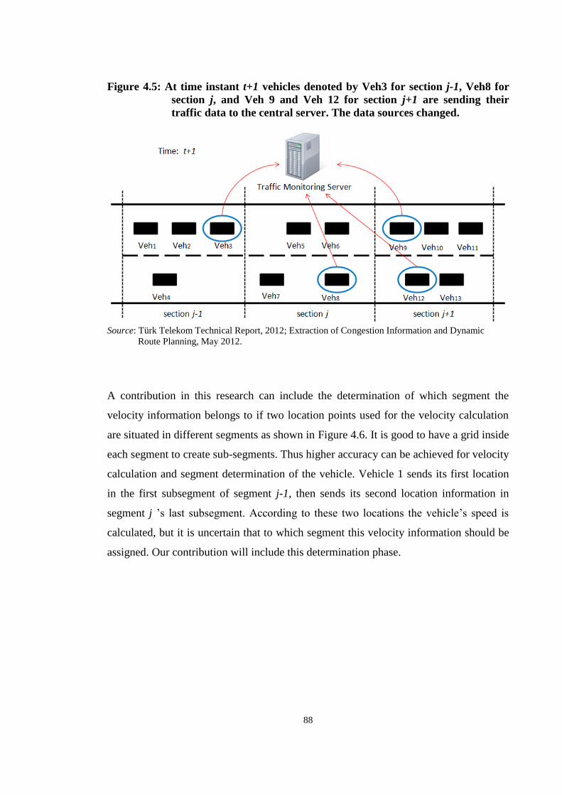
88
Figure 4.5: At time instant t+1 vehicles denoted by Veh3 for section j-1, Veh8 for
section j, and Veh 9 and Veh 12 for section j+1 are sending their
traffic data to the central server. The data sources changed.
Source: Türk Telekom Technical Report, 2012; Extraction of Congestion Information and Dynamic
______ Route Planning, May 2012.
A contribution in this research can include the determination of which segment the
velocity information belongs to if two location points used for the velocity calculation
are situated in different segments as shown in Figure 4.6. It is good to have a grid inside
each segment to create sub-segments. Thus higher accuracy can be achieved for velocity
calculation and segment determination of the vehicle. Vehicle 1 sends its first location
in the first subsegment of segment j-1, then sends its second location information in
segment j ’s last subsegment. According to these two locations the vehicle’s speed is
calculated, but it is uncertain that to which segment this velocity information should be
assigned. Our contribution will include this determination phase.

89
Figure 4.6: Processing the location data for velocity calculation in case that
vehicles report their successive data in different road segments.
Source: Türk Telekom Technical Report, 2012; Extraction of Congestion Information and Dynamic
______ Route Planning, May 2012.
Another question is about how we should store the data coming from vehicles equipped
with GPS-enabled smartphones. We could use a table like below but it is still an
essential question how to fill the data in the table. Segment specific velocity values can
be calculated by using the interpolation methods on the data coming from different
vehicles for each segment and/or sub-segment.
Table 4.1: Storing the data coming from the smartphones in floating cars
1 1 2 2 3 3 4 4 5 5
Car 1 0 75
Car 2 0 60
Car 3 0 30
Car 4 0
Car 5 0
Source: Türk Telekom Technical Report, 2012; Extraction of Congestion Information and Dynamic
______ Route Planning, May 2012.

90
The design introduced here resembles in many ways to that in wireless sensor networks.
We could use the simulation environments in sensors networks with a few modifications
applied. In sensor networks the sensors or the actuators report their data in three ways:
a. Periodic: E.g. 1 min time intervals ( )
b. Threshold: E.g. 20 meters distance ( )
c. Combined: E.g. (10 min, 20 meters)
In these networks, there is a sink node that every sensor or actuator forwards its data to
be processed or further sent to a central server. Figure 4.7 illustrates a sample scenario
in sensor networks where every sensor node sends its data to the sink, and the sink
forwards the data to the server.
Figure 4.7: Resemblance of the floating vehicle reports with the Wireless Sensor
Networks
Source: Türk Telekom Technical Report, 2012; Extraction of Congestion Information and Dynamic
______ Route Planning, May 2012.
It is also possible to address the average velocity calculation issue utilizing the micro-
grids in each section, as depicted in Figure 4.6. There are three methods considered for
the calculation process.

91
4.3.1 Methods for Average Velocity Calculations
This section presents the studies in order to address the average velocity
calculation issue utilizing the micro-grids in each section, as depicted in Figure 4.6.
There are three methods considered for the calculation process.
4.3.1.1 First method
The method consists of dividing the known velocity into micro-grids, and then finding
the overall velocity by averaging the velocities identified by each micro-grid.
The method includes the following considerations:
a. The incoming data must correspond within a time interval denoted by and a
± threshold which can provide a specific precision in time.
b. If the data does not belong to this time interval, then the data is obsolete, thus
must be retired.
The model and an example are depicted in Figure 4.8. In this example, the average
velocity that belongs to the first section of the road is tried to be calculated, where there
are three vehicles associated with the first section and their velocity are 60 km/h, 70
km/h, and 65 km/h for V1, V2, and V4, respectively. However all of the cars are also
associated with section 2, as well. This situation pops up the question that which section
does the vehicle velocities belong to. The method tries to address the problem by:
i. Divide the section into micro-grids.
ii. Determine which vehicles are located in which micro-grid.
iii. For each micro grid, calculate the average velocity using the vehicles’
velocities in the micro-grid.
iv. Calculate the overall velocity by averaging the velocities calculated for each
micro-grid.
The mathematical representation of the method is as following:
: Micro-grid index
: Section index
: Vehicle index
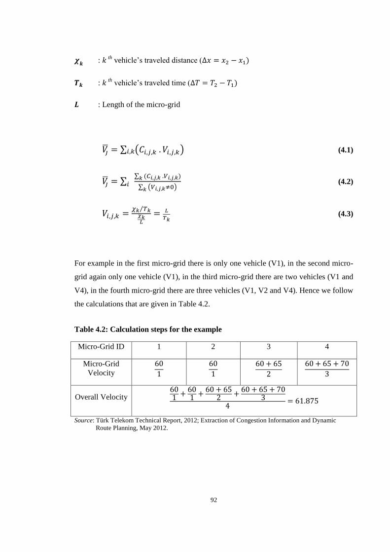
92
: th vehicle’s traveled distance (
: th vehicle’s traveled time (
: Length of the micro-grid
∑ ( ) (4.1)
∑∑
∑ ( ) (4.2)
⁄
(4.3)
For example in the first micro-grid there is only one vehicle (V1), in the second micro-
grid again only one vehicle (V1), in the third micro-grid there are two vehicles (V1 and
V4), in the fourth micro-grid there are three vehicles (V1, V2 and V4). Hence we follow
the calculations that are given in Table 4.2.
Table 4.2: Calculation steps for the example
Micro-Grid ID 1 2 3 4
Micro-Grid
Velocity
Overall Velocity
Source: Türk Telekom Technical Report, 2012; Extraction of Congestion Information and Dynamic
______ Route Planning, May 2012.
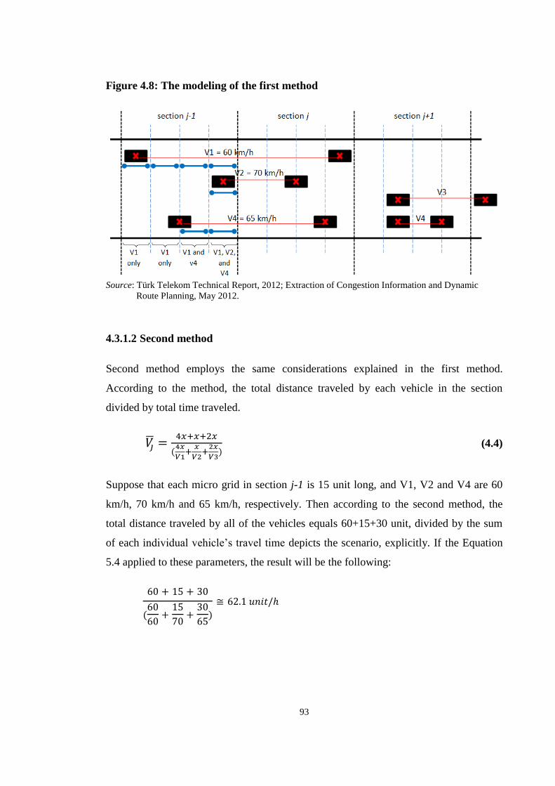
93
Figure 4.8: The modeling of the first method
Source: Türk Telekom Technical Report, 2012; Extraction of Congestion Information and Dynamic
______ Route Planning, May 2012.
4.3.1.2 Second method
Second method employs the same considerations explained in the first method.
According to the method, the total distance traveled by each vehicle in the section
divided by total time traveled.
(4.4)
Suppose that each micro grid in section j-1 is 15 unit long, and V1, V2 and V4 are 60
km/h, 70 km/h and 65 km/h, respectively. Then according to the second method, the
total distance traveled by all of the vehicles equals 60+15+30 unit, divided by the sum
of each individual vehicle’s travel time depicts the scenario, explicitly. If the Equation
5.4 applied to these parameters, the result will be the following:

94
Figure 4.9: Model and an example for the second method
Source: Türk Telekom Technical Report, 2012; Extraction of Congestion Information and Dynamic
______ Route Planning, May 2012.
4.3.1.3 Weighted moving average method
The weighted moving average method consists of assigning a weight factor on the
average velocity calculation:
(4.5)
4.4 ANDROID APPLICATION: TTRAFFIC
We need real-life data to be used in our simulations. For this purpose, we decided to
develop an Android application named TTraffic that will do the following tasks:
a. Saving the location information (longitude, latitude, altitude) and timestamp for
each successive data received from the GPS satellites in a file. In addition, it also
calculates the velocity for each pair of data using the simple equation (distance
traveled divided by time difference) and saves it into the same file.

95
b. Get the speed values using the android.location.Location.getSpeed() method
(along with hasSpeed()) in our LocationListener implementation. Then these
values will be compared with the values from conventional speed calculation.
This mobile application (TTraffic) is developed by the same research group as part of
the Türk Telekom R&D Projects and presented as the capstone project of an
undergraduate student. However it is not mentioned in detail within the scope of this
thesis.
4.5 OPTIMIZATION AND CALIBRATION PHASE
4.5.1 Determining the Fixed Time Interval for Data Transfer
We will let the user to select the frequency of sending the GPS data to the central server.
The more frequent the user sends data to the system, the more frequent updates about
the traffic congestion status he/she will get from the system. This way the users will be
motivated to participate actively on the evolution of the system.
4.5.2 Sending the Data When the Speed Band Changes
Another option to determine when to send the data to the central server is to inspect the
significant changes in speed of the vehicle. Consider that there are pre-determined speed
bands A, B, C, D and E as shown in color-speed scale in Table 4.3. The vehicle might
send its data to the traffic monitoring server only if its speed band changes. In other
words, if the change in the vehicle’s speed reflects a significant amount then the vehicle
should send the data, or vice versa.
Table 4.3: Color-Speed scale
Speed 90+ 89-70 69-50 49-30 29-0
Color Scale A B C D E
Source: Türk Telekom Technical Report, 2012; Extraction of Congestion Information and Dynamic
______ Route Planning, May 2012.
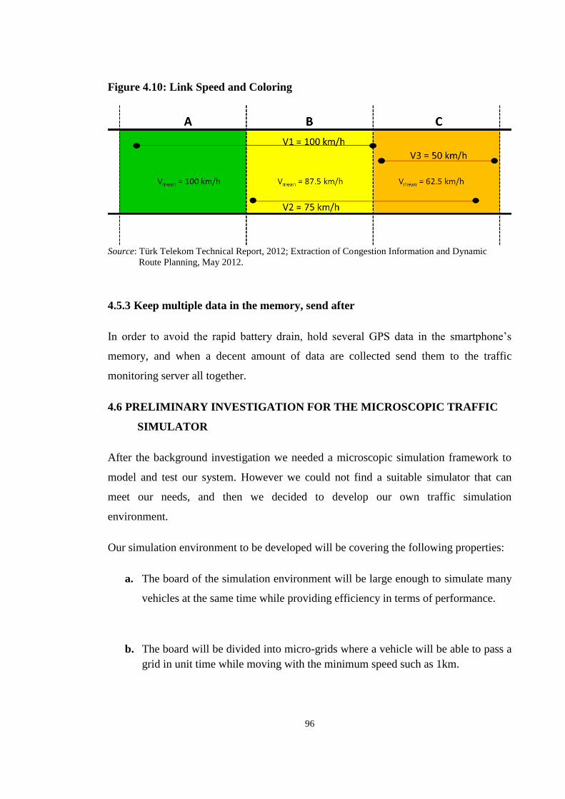
96
Figure 4.10: Link Speed and Coloring
Source: Türk Telekom Technical Report, 2012; Extraction of Congestion Information and Dynamic
______ Route Planning, May 2012.
4.5.3 Keep multiple data in the memory, send after
In order to avoid the rapid battery drain, hold several GPS data in the smartphone’s
memory, and when a decent amount of data are collected send them to the traffic
monitoring server all together.
4.6 PRELIMINARY INVESTIGATION FOR THE MICROSCOPIC TRAFFIC
SIMULATOR
After the background investigation we needed a microscopic simulation framework to
model and test our system. However we could not find a suitable simulator that can
meet our needs, and then we decided to develop our own traffic simulation
environment.
Our simulation environment to be developed will be covering the following properties:
a. The board of the simulation environment will be large enough to simulate many
vehicles at the same time while providing efficiency in terms of performance.
b. The board will be divided into micro-grids where a vehicle will be able to pass a
grid in unit time while moving with the minimum speed such as 1km.

97
c. E.g. consider that with minimum speed 1km/h the number of grids that is
traveled in unit time is 1 grid, and then with 80km/h the distance traveled will be
80 grids.
d. If the board size is 600x600 pixel, then the number of pixels a single micro-grid
corresponds to will be evaluated and scaled accordingly. Because otherwise, it
would take only a few unit times to travel the whole board from beginning to the
end, even for the vehicles that move slowly. Scaling, in this way, will allow for a
zoomed-out board display.
e. E.g. Considering a micro-grid would correspond to 0.01 pixel, then the whole
road for a 600 px wide board would be 60000 micro grids, and that can be
traveled in 60000 unit times with the velocity of .
f. The board will have a variable that will control the number of lanes in sections.
Figure 4.11: Demo of vehicles’ micro-grid positions at times t1, t2, t3, t4, t5
depending on their varying speed at each unit time
g1 g2 g3 g4 g5 g6 g7 g8 g9 g10 g11 g12 g13 g14 g15 g16 g17 g18 g19
Veh1 t1 t2 t3
t4 t5
Veh2 t1 t2 t3 t4 t5
Veh3 t1 t2
t3 t4 t5
Source: Türk Telekom Technical Report, 2012; Extraction of Congestion Information and Dynamic
______ Route Planning, May 2012.
g. The vehicles will be arbitrarily generated at random lanes (y coordinates) and at
random times.
h. The lanes will have 3 meters width; hence random lanes that the vehicles will be
in will be having fixed differences of 3 meters and multiples of 3.
i. The vehicles will move with varying speeds, so there will be a possibility of
collision. When collision occurs they will stop.

98
j. The number of vehicles that will start moving on the roadway will also be
another simulation parameter.
4.7 SENSOR NETWORK ANALOGY AND DATA ACQUISITION FROM
EACH SEGMENT
Improving the sensor model described in Figure 4.7 we introduce the case where there
may be many sensors in each segment, however we are not able to receive data from
some of them or they would not send their data due to following reasons:
i. Battery is depleted
ii. Does not prefer sending the data
iii. Forgot to or did not want to run the application
iv. Only a few have the application in the segment
Figure 4.12: The case where many nodes are unable to send the data by the
analogy of sensor networks
Source: Türk Telekom Technical Report, 2012; Extraction of Congestion Information and Dynamic
______ Route Planning, May 2012.
4.7.1 Exploiting Base Station Hand-Offs
There is also another notion that is based on exploiting the cell phone signals during the
hand-offs between the base stations. In such systems the users need not know about an
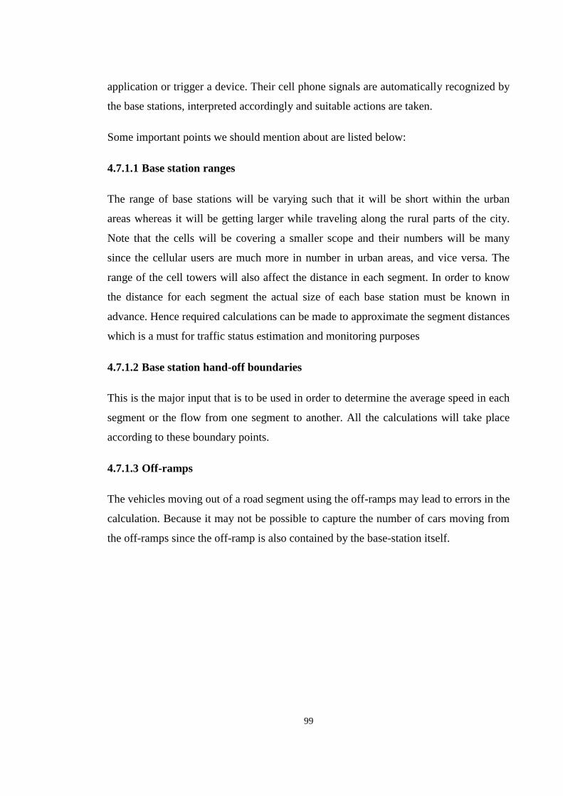
99
application or trigger a device. Their cell phone signals are automatically recognized by
the base stations, interpreted accordingly and suitable actions are taken.
Some important points we should mention about are listed below:
4.7.1.1 Base station ranges
The range of base stations will be varying such that it will be short within the urban
areas whereas it will be getting larger while traveling along the rural parts of the city.
Note that the cells will be covering a smaller scope and their numbers will be many
since the cellular users are much more in number in urban areas, and vice versa. The
range of the cell towers will also affect the distance in each segment. In order to know
the distance for each segment the actual size of each base station must be known in
advance. Hence required calculations can be made to approximate the segment distances
which is a must for traffic status estimation and monitoring purposes
4.7.1.2 Base station hand-off boundaries
This is the major input that is to be used in order to determine the average speed in each
segment or the flow from one segment to another. All the calculations will take place
according to these boundary points.
4.7.1.3 Off-ramps
The vehicles moving out of a road segment using the off-ramps may lead to errors in the
calculation. Because it may not be possible to capture the number of cars moving from
the off-ramps since the off-ramp is also contained by the base-station itself.

100
Figure 4.13: Depiction of hand-offs between base stations and the off-ramp / on-
ramp problem
Source: Türk Telekom Technical Report, 2012; Extraction of Congestion Information and Dynamic
______ Route Planning, May 2012.
4.8 BAU REAL-TIME TRAFFIC SIMULATOR
In the second phase of the research, a microscopic traffic simulator is needed to be
developed in order to provide both a test and a display mechanism of the traffic system.
The name of the simulator is BAU Real-time Traffic Simulator. This simulator will not
only provide the required data to be used in the research analyses, but also play the role
of the research method.
Simulator is written in Java development environment since it handles the threaded
software development quite well and the ability to run in multi-platform, i.e. in multiple
operating system platforms.
4.8.1 Motivation
The main reason that leads to the idea of a Smart Transportation Simulator is to develop
a framework to analyze and test our GPS data retrieved from the test vehicles on the
field that use our Android application. The simulation will allow us the possibility to
create road sections with specified number of lanes in each of them. Hence we will be

101
able to find out the average velocity and density for each section on the roadway that is
to be simulated.
The traffic simulator is focused on achieving several aims as listed below:
a. Test the data collected by the android smartphone app TTrafic.
b. Generate random runtime data for various setups (e.g. Dynamic random 100
vehicles in each section of a four section roadway with varying lengths) and plot
them for analysis purposes.
c. Calculate the traffic conditions according to the data received from the built-in
GPS sensors within the smartphones.
d. Simulator’s output is the smartphone app’s input: Use these data to determine
the section traffic congestion weights and paint the section colors on the map
displayed in the smartphone app.
e. Simulator’s input is the smartphone app’s output: Display the output of the end-
user data transmitted by the android app TTraffic from within the user vehicles
(display vehicle locations on the traffic map)
f. Simulate the battery model
4.8.2 The System Architecture
The simulator is based on 7 classes. These classes can be listed as:
i) Vehicle, ii) Battery, iii) Section, iv) RandomVehiclesThread, v) Board, vi)
Configuration, vii) Simulation.

102
This section presents the class tasks and the smart phone battery model implemented in
the system, as well as the class diagrams that show the interactions between the classes.
4.8.2.1 The Battery Consumption Model
a. The battery will be shown as a percentage level for each vehicle.
b. Each phone may have different percentage of initial battery power when the
mobile application is run. In the simulation scenarios the battery level will either
be randomly chosen or set as 100 percent in the start.
c. The mobile application will consume a constant amount of power in the
background even though it is in the idle state.
d. The battery model in the simulator will have another consumption state where
the user is having a call at the same time the mobile application is running. A
real test is run in order to find out the approximate level of battery power the
phone consumes during this state.
e. When the mobile application is run by a smart device it will require a constant
amount of start-up power, e.g. 1 percent.
f. Each data transmission by the smart devices in the floating vehicles will drain an
approximate amount of power from the battery, e.g. 0.01 percent. In other
words, such an amount of power is consumed in each iteration of the traffic
simulator.
g. Real-time or predicted map requests from the server will drain 0.5 percent
battery power.
h. If the vehicle charger connection is established it will not drain the battery. On
the contrary it will charge the battery with a certain amount of replenishment
rate, e.g. 0.8 percent per minute, as long as the battery level is lesser than 100
percent.

103
4.8.2.2 Classes
The classes and their distinct responsibilities together with their interaction are
presented in great detail in this section. The classes are designed according to the known
design principles and design patterns to provide desirable features such as reusability,
readability, extendibility, etc. However, further abstraction on these classes are possible
to be implemented if required.
4.8.2.2.1 Class Diagram
Seven classes are developed in this simulator software. The structure of the software is
designed in such a way that it is open for extension instead of modification. The
software can be equipped with further tasks to perform when it is desired. The scope of
the simulator suggests a class diagram as shown in Figure 4.14.

104
Figure 4.14: Comprehensive class diagram of the BAU Traffic Simulator
Source: Türk Telekom Technical Report, 2012; Extraction of Congestion Information and Dynamic
______ Route Planning, May 2012.

105
4.8.2.2.2 Vehicle
Vehicle class is basically responsible of creating a vehicle to be painted on the main
panel as well as keeping track of the vehicle’s most important attributes such as its id, x
and y coordinates, speed and the current section at any time instant. Other major roles
include the operational steps to be executed during the vehicle movement, application
startup, charger connection and disconnection, congestion map requests, data
transmission to the server, section decisions, speed changes, and picking the random
vehicle display image.
Vehicle class extends the Thread class as its parent class. Hence a run() method is
implemented for the Vehicle class. The task of the thread is determined within this
method. This is the point where the vehicle will not only move (i.e. set its new location)
according to its instantaneous speed, but also will decide what section it is in after the
movement. Moreover the thread will help the vehicle change its speed randomly, i.e.
accelerate or decelerate. Such operations implemented as the thread task will be
executed in each time interval that is specified by the static field
updateVehicleLocationFrequency in the Configuration class.
Vehicle class has 12 fields of varying types. These fields can be listed as below:
a. battery: It is a reference on a Battery object. With the help of this field, the
battery is consumed or charged according to the operation performed by the
Vehicle. These operations can be one of the following i) appStartUp(), ii)
transmitDataToTheServer(), iii) requestCongestionMap(), iv)
connectPhoneToCharger().
b. count: This field is responsible for counting the vehicle objects created during
the simulation and is of the primitive type int. It is a static field of the Vehicle
class, hence the id of the vehicle can be assigned on the vehicleId field.
c. image: image is a reference on an object of the type Image. It is assigned with a
randomly chosen image that displays the vehicle on the simulator panel.

106
d. imageList: this field is a static string array that has the names of the vehicle
images present in the simulator. It is used by the pickRandomImage() method.
e. locationX: This field keeps the pixel value for the x coordinate of the vehicle as
the double primitive type. Actually this value is scaled according to the
simulator screen and the vehicle’s reported coordinate on the road. It is then
used as the upper-left corner coordinate of the randomly chosen vehicle’s
bounding rectangle.
f. locationY: This field keeps the pixel value for the y coordinate of the vehicle as
the double primitive type. Actually this value is set according to the lanes in
which the vehicle is located at the time being. It is then used as the upper-left
corner coordinate of the randomly chosen vehicle’s bounding rectangle. Its value
is specifically assigned in such a way that the vehicle will eventually appear
within one of the lanes of the current section.
g. okToRun: There is a Thread assigned for each vehicle that is started to run on
the creation time. When it is true, the thread task operation will continue. When
it is false, the thread will stop and hence the vehicle movement will stop.
h. rndImage: This static field is of a Random type and is used in
pickRandomImage() method to pick the random image from the imageList string
array.
i. rngSpeed: This is also of the type Random and is used for deciding how the
vehicle will move in the current iteration of the thread. The vehicle can
accelerate and decelerate. Both acceleration and deceleration can happen at three

107
levels, i.e. plus or minus 1 or 2 or 3 magnitudes of speed change on the current
speed.
j. speed: The speed level is the primitive type double and is determined to be
between 1 km/h and 120 km/h. If somehow the speed drops below 1 km/h or
exceeds 120 km/h it will then be set to minimum or maximum values
appropriately by the changeSpeed() method. Each vehicle has its own speed
randomly set on the object (vehicle) creation process. The speeds are determined
for each vehicle according to the section it is in at the time it is created. For
example if the vehicle is in first section and the first section’s initial speed
interval was set as between 40 km/h and 60 km/h in the Configuration class,
then the speed will be randomly chosen between these values as the minimum
and the maximum limits.
k. sectionNo: This field is initially set when the vehicle is created anywhere on the
screen. The section is determined according to the creation location or the
section that uses the Section class’s accept(Vehicle v) method. When a section
gets the vehicle as the parameter inside the accept(Vehicle v) method, that
vehicle’s sectionNo is set with the id of that specific section. This is an
important field that plays a key role on the section decision operations
throughout the simulator software.
l. vehicleId: This field also plays a key role on the vehicle list updates for each
section. The vehicles are added in or removed from a section according to the
unique vehicleId. Actually hascode() and equals() methods are overriden
according to the "vehicleId" field of the Vehicle class, so that the predefined
methods that utilizes equals() or contains() methods will behave according to
this criteria.
Other than the 12 fields, there are 9 getter methods and 7 setter methods. Getter
methods are comprised of getBattery(), getImage(), getLocationX(), getLocationY(),

108
getSectionNo(), getSpeed(), getVehicleId(), isOkToRun(). On the other hand, the setter
methods can be listed as setBattery(), setImage(), setLocationX(), setLocationY(),
setSectionNo(), setSpeed(), setVehicleId().
Furthermore, the constructor and the remaining methods are explained below in detail:
i. Vehicle(double speed, double locationX, double locationY, Battery battery):
There is just a single constructor for Vehicle class and it gets four parameters in
it. It simply sets the vehicleId field according to the count static field by
increasing this value every time the constructor call is made, i.e. every time a
vehicle object is created. After that, the vehicle’s speed field, locationX and
locationY fields, battery field are set according to the incoming parameters. The
vehicle’s image is also set with the random image returned by the
pickRandomImage() method.
ii. void run(): It is an @Override method specified by the Thread class and is
implemented by the child class, namely Vehicle. According to the run() method,
what kind of tasks the implementing class should carry out is determined.
Vehicle’s thread is responsible for the specific vehicle’s movement operation
according to its instantaneous speed. A Boolean variable, namely okToRun is
used in order to stop this thread or make it keep running, in other words keep the
vehicle moving. Other than the movement task, the thread also commands the
vehicle to decide its new section if it has changed, and change the vehicle’s
speed. These tasks are performed in each time interval the Configuration class
specified with updateVehicleLocationFrequency field. The thread actually sleeps
for the amount designated by that field. The thread also sleeps only once when it
is started() for the very first time.
iii. void appStartUp(): This method is responsible of doing everything specifically
needed at the smart phone application startup time. Other than that, it executes
the consumeTransmitPower() method located in Battery class which is accessed

109
from its battery field, if and only if the battery is not docked into the vehicle
charger.
iv. void transmitDataToTheServer(): Do whatever is needed in the transmission
to the server process. Morever, as long as the vehicle charger connection is not
established consume the battery for the amount needed in
battery.consumeTransmitPower() method of the Battery class. There will be no
battery consumption if the smartphone, and thus the battery, is connected to the
charger.
v. void requestCongestionMap(): Execute the operations to request the
congestion snapshot from the server. In addition, if the smartphone is not being
charged then consume the battery for the amount needed in
battery.consumeMapRequestPower() method of the Battery class. Of course
again, no battery consumption is performed if it is connected to the charger.
vi. void connectPhoneToCharger(): Execute the charge method implemented
within the Battery class. Use the vehicle’s battery field to access to the method.
vii. void unplugPhoneFromCharger(): This method simply calls the
battery.unplug() method which stops the thread responsible of the charging task
within the Battery class.
viii. void changeSpeed(): This method uses a switch that generates a random
number over six states. According to the number, it decides at which level the
vehicle should accelerate or decelerate. It is performed by increasing the speed
value by +1 or +2 or +3; or similarly decreasing the speed value by -1 or -2 or -
3. Check if the speed value is between 1 and 120 km/h. If not set the value to 1 if
it is lower than 1 or 120 if it is greater than 120.

110
ix. void decideSection(): This method is called after each movement in the
vehicle’s thread. When the location is updated, check to see if the new section is
different than what the current sectionNo shows. It is decided by the section
boundary locations that are dynamically determined according to the number of
sections and their lengths present in the simulation setup. If the section was
changed, remove this vehicle from the previous section’s vehicle list and all the
other vehicle lists related to that section. After that, check if it is the last section
in the simulation setup, if it is then stop this vehicle’s thread so it will stop and
disappear on the simulation screen. If it is not the last section then accept this
vehicle to the next section, i.e. to the new section.
x. boolean equals() & int hashCode(): These are the overridden hashCode() and
equals() methods that use the vehicleId in order to override the comparison
mechanism for the vehicle objects. These are java specific implementations
modified for the Vehicle class.
xi. String pickRandomImage(): Decides on a random image from the image list.
Thus the created vehicle will have that specific image to depict the vehicle on
the simulation screen.
As it is also shown in the class diagram in Figure 4.15, Vehicle class depends upon
Board class and Board class depends upon Vehicle class. Vehicle also depends upon
Configuration class that has just static fields. Another class that depends upon Vehicle is
RandomVehiclesThread.
Besides, Vehicle class references one Battery object, whereas both
Section.randomVehiclesArray and Section.vehicleList references many Vehicle objects.
111
Figure 4.15: Vehicle class’s structure
Source: Türk Telekom Technical Report, 2012; Extraction of Congestion Information and Dynamic
______ Route Planning, May 2012.

112
4.8.2.2.3 Battery
Battery class plays the role of a smartphone battery which is consumed by the
operations done on the client side. Using the battery class aims at simulating the battery
consumption model while transmitting and receiving data during the communication
processes.
Every vehicle has a smartphone and hence a battery integrated with it. The Board class
creates the vehicles using the generateRandomVehicles(Section s, int min, int max)
method for the specified section within random speeds bounded by the lower and upper
limits defined by the min and max values. Every vehicle is created with the random
speed range specified, at the specified X and Y coordinates (Y coordinate stands for the
lane number) including a battery with arbitrary level of energy stored in it. Thus it
makes the Vehicle class dependent on the Battery class.
Battery class extends the Thread class that makes it responsible of executing a task in its
run() method. The task is based on the charge() method. The charge method starts the
charging process that increases the battery level by 0.8 percent in each charge frequency
defined in the Configuration.chargeFrequency static field. When the battery level is
greater than or equal to100 percent it simply keeps the charging without increasing the
battery level. The other major roles are composed of unplugging from the charger,
consuming the application startup power, consuming the transmission power, and lastly
consuming the energy needed for real-time map requests.
Vehicle class has only two fields. These fields are listed below:
a. level: The field is of a double type and is used for keeping the battery state in
terms of percentage levels. Every method uses this level field such that they
either decrease or increase the value by a certain percentage determined during
the battery analyses using an android phone.
b. isConnectedToCharger: This field is the type of a boolean. It is used to check
the state of the charger connection. The actual purpose it has is to either stop the
loop in the run() method that is responsible for charging the battery when the

113
charger connection is established, or to keep the thread (charging operation)
running.
Moreover, the class has both setter and getter methods assigned to each fields. These
methods have the name: getLevel(), setLevel(double level), isConnectedToCharger(),
setIsConnectedToCharger(Boolean isConnectedToCharger).
Furthermore, the class has one parametric constructor as well as 6 other methods
including the thread’s run() method. The methods are comprehensively explained
below:
i. Battery(double level, Boolean isConnectedToCharger): the Battery objects
are instantiated using the parametric constructor Battery(double level, Boolean
isConnectedToCharger). The constructor simple sets the initial battery level (in
the simulation runs it is set as 100 percent in vehicle creation phase) and checks
if the isConnectedToCharger field is true or not, and if it is true the charge()
method is called.
ii. void charge(): The charge() method simply starts the thread’s run() method that
increases the battery level by 0.8 percent in every minute. Right before the
thread is started, isConnectedToCharger field is set as true since the charge()
method can be called arbitrarily outside the constructor.
iii. void unplug(): The method actually acts as a setter method. It simply sets the
value of isConnectedToCharger field to false, hence the thread stops running.
iv. void consumeAppStartUpPower(): The method is used to decrease the battery
level by the amount specified within the method. This method is used when the
RandomVehiclesThread's run() method is executed in every n
(renewRandomVehiclesPeriod) seconds. This means that the vehicles will only
consume app startup power whenever they start their applications in every n

114
(renewRandomVehiclesPeriod) seconds. If the battery level is somehow
decreased to a level lesser than zero, it will set the remaining battery level to
zero, hence prevent the possibility of setting negative values.
v. void consumeTransmitPower(): The method decreases the value assigned to
level field by an amount defined in the method, e.g. 0.01 percent.
consumeTransmitPower() method is called in each repaintFrequencyInMillis,
i.e. the frequency of the time which the vehicles transmit their data. By design,
the transmission to server occurs whenever the vehicles’ new locations are
updated, in other words repainted. It guarantees that the remaining level is
greater than or equal to zero.
vi. void consumeMapRequestPower(): This method is also responsible of
decreasing the battery level by an amount defined in the method, e.g. 0.5
percent. consumeMapRequestPower() is used in each repaintFrequencyInMillis,
i.e. the frequency of the time which the vehicles transmit their data, as well.
Because the system tries to reward the user and hence keep their congestion map
up-to-date whenever the user contributes in the system by transmitting its GPS
data (location and speed) to the server. This method also guarantees that the
remaining level is greater or equal to zero.
Figure 4.16 introduces the class diagram for the Battery. Battery class depends upon
Configuration class since it uses the static field chargeFrequency defined in it.

115
Figure 4.16: Battery class’s structure
Source: Türk Telekom Technical Report, 2012; Extraction of Congestion Information and Dynamic
______ Route Planning, May 2012.
4.8.2.2.4 Section
Section class has a very active role in the simulator software. It has several important
responsibilities. Besides, many of the other classes depend upon the vehicle lists saved
by the section objects.
Section class helps to create the virtual boundaries drawn on the simulation field, as
well as keeping track of the starting and ending coordinates and distances of each
section iteratively created. Basically, the whole simulator waits for the average speed
calculations done and then saved in each section object. The class accepts the vehicles
that enter from the objects starting boundary, and removes the vehicles that are passing
from the ending boundary point of the corresponding section object. Hence the vehicle
list is properly determined and is provided to dependent methods and classes for further
operations.
Major roles of the Section class are accepting a vehicle into the section, removing the a
vehicle from all the vehicle lists saved in the section, calculating the density in the
section, calculating the real average speed in the section, calculating the average speed

116
of the transmitting vehicles in the section at a specific time instant, calculating the
average speed of a specific vehicle list given as an input, writing the average speed of
all vehicles as well as the average speed of randomized vehicle lists into a file for the
section, filling the random vehicles arrays as well as the average speed analyses arrays,
determining the section color according to the average speed of the vehicles in the
section, and saving the latest available section speed in order to show it in case a
problem occurs.
The Section class has 18 fields of varying types of which two of them are static. The
fields are explained thoroughly below:
a. startPosition: This is a static field of the type integer. It basically starts with the
value of zero and increased by the length of the latest section object created.
This way the starting and the ending distances of the next section to be created
can be determined easily on the complete roadway.
b. count: Every section has a sectionId to make the sections unique. The count
field is a static field and increased by one every time a new section object is
created, and thus the sectionId is determined using this static integer field named
count.
c. density: Every section can have not only different lengths but also different
number of vehicles present in it. The field density is used to provide a statistical
ratio that keeps track of the number of vehicles per kilometer (vpk) in a section
as a double type value. The field is one of the key parameters used in the traffic
theory which provides an approximate comparison metric.
d. averageSpeed: The users in a real-time traffic system wonder how congested
the sections are and evaluate the congestion levels according to the average
speed measurements given for the sections. For this reason, the average speed
field in a section is quite important. This field is of the type double and is

117
responsible for keeping track of the average speed of all vehicles present in the
section. This is the real average speed that describes the section and can be
compared with the average speed calculated for the vehicles contributing into
the system by transmitting their locations and speeds to the server. The average
speed is kept in terms of km/h.
e. previousAverageSpeed: This field saves the latest average speed of all vehicles
in the section in case a problem occurs during the calculation and thus the latest
average speed value can be shown instead. It is also of the type double and is
saved in terms of km/h.
f. randomVehiclesAverageSpeed: It is basically the same as averageSpeed field.
The type of the field is double and keeps the value in terms km/h. But this
average speed is calculated using the random vehicles list that stands for the
vehicles that are selected for transmitting data to the server.
g. sectionId: The field is of the type integer and its value is assigned by the static
field count. This field is used to determine the unique sections.
h. startX: This field is an integer type, as well. The field saves the actual starting
point of the section in the x axes in terms of real distances in a straight roadway.
Its value is assigned by the startPosition static field which is updated everytime a
section is created.
i. endX: This field has exactly the same properties as startX. The only difference
is that it saves the meter value of the actual ending point of the section in the x
axes in terms of real distances in a straight roadway. Its value is determined by
the sum of startX and the section length.

118
j. startXBoundary: It keeps track of section's starting vertical boundary as exact
pixel coordinates on the painted area (Board JPanel). The values are scaled
accommodate the drawing area. Thus startXBoundary is assigned with the value
calculated by Simulation.B_WIDTH static field minus the half of the startX.
k. endXBoundary: It keeps track of section's ending vertical boundary as exact
pixel coordinates on the painted area (Board JPanel). A scaling process which is
the same as in startXBoundary calculation is done. Thus endXBoundary value is
determined by Simulation.B_WIDTH value minus the half of endX value.
l. sectionColor: This field is of the type Color and is responsible for saving the
color state of the section. The color of the section is assigned by the
getSectionColor(Graphics g) method located in the Section class. It simply
checks the average speed of the section and assigns the appropriate color
according to the the average speed value. The details are given in
getSectionColor(Graphics g) method.
m. writer: writer keeps a reference to a PrintWriter object. The field than
instantiated with a PrintWriter object that takes a new file object as a parameter
whose name is determined by the sectionId, in the Section’s constructor. In
short, every section creates its own file to log the average speed calculations in.
It is used in the writeAverageSpeedAndRandomVehiclesAverageSpeedToFile()
method.
n. vehicleList: This is the most important field in the whole program. Because the
output of the simulator totally depends on this List of the type Vehicle. The field
has a reference to a synchronized array list and is instantiated in the same line it
is defined. According to the vehicles accepted in or removed from the section,
the corresponding vehicleList field is updated. The average speed calculations
are done in each iteration according to the vehicles present in the section’s

119
vehicleList field. This field is the key to many classes and methods written in the
simulator software.
o. randomVehiclesArray: This field has the same properties as vehicleList field.
But this array list contains the vehicles that are selected randomly for
transmitting their data to the server. The upper average speed labeled as “Rnd
Avg Speed” in the simulator interface is calculated using this List of the type
Vehicle.
p. averageSpeedAnalysesArray: This field is an Array List containing multiple
Lists of the type Vehicle. The field actually keeps a reference to the Lists of
dynamic random 20, dynamic random 40, dynamic random 60 and dynamic
random 80 vehicles, which are mentioned throughout the dynamic random
analyses. These average speeds are calculated and written in to the section files
in the third, fourth, fifth and sixth columns for dynamic random 20, dynamic
random 40, dynamic random 60 and dynamic random 80 vehicles, respectively.
Moreover, the class has 15 setter and getter methods in total. Some fields have only
getter method while some others have both getter and setter methods. These methods
are, namely: getLength(), setLength(int length), getNumLanes(), setNumLanes(int
numLanes), getStartX(), setStartX(int startX), getEndX(), setEndX(int endX),
getStartXBoundary(), getEndXBoundary(), getSectionId(), getWriter(),
getPreviousAverageSpeed(), getRandomVehiclesArray(), getVehicleList().
Furthermore, the class has one parametric constructor as well as 9 other methods. The
methods are explained comprehensively below:
i. Section(int length, int numLanes): The parametric constructor gets two
parameters in total, one of which is to set the length of the section (given in
meters) and the other is to set the number of lanes. The constructor first of all
sets its sectionId according to the value taken from the static field count. After
that the average speed and the previous average speed values are initialized to
zero, and then the writer is instantiated to a PrintWriter that writes into a file

120
corresponding to the same section id. Then the length of the section is checked
and tuned. The sections must be larger than 300 meters in order to assure that the
distance that can be travelled within a cycle of update time does not exceed the
minimum section length. In the following lines, the number of lanes is checked.
The number of lanes for a section cannot be lesser than 1 and greater than 8. If
the number of lanes is outside of this range appropriate adjustments are done.
Then the startX and endX values are set using the startPosition static field and
the length field. Furthermore the startXBoundary and endXBoundary values are
scaled and set according to the aforementioned calculations. Lastly the
startPosition static field is updated with the latest value of endX field, and
required number of new synchronized array lists of the type Vehicle are added
on the averageSpeedAnalysesArray field.
ii. void acceptVehicle(Vehicle v): This method is responsible for the operation of
adding the Vehicle v taken as a parameter into the section’s vehicleList. Besides
the vehicle’s section id is set with the value coming from the getter method
this.getSectionId().
iii. void removeFromAllTheVehicleArrayLists(Vehicle v): This method is called
in the Vehicle class’s decideSection() method. When a vehicle changes its
section during the movement process, it takes action to determine its new section
using the decideSection() method. Firstly vehicle must be removed from all the
vehicle lists it appeared previously, and then the new section is determined
appropriately. These vehicle lists are namely the vehicleList, and all the lists in
the averageSpeedAnalysesArray.
iv. double getDensity(): The method basically checks the section’s vehicleList if it
is empty or not. If it is empty it return zero, and if not then it sets the density by
dividing the number of the vehicles in the list by the length of the section, and
returns this value.

121
v. double getAverageSpeed(): Average speed calculation of all the vehicles
present in the section is performed by this method. The method first of all
checks if the vehicleList is empty, if not it sums up the vehicle speeds and
divides it to the number of vehicles and return the result. Meanwhile the value of
previousAverageSpeed is also assigned. If there are no vehicles the average
speed is set to zero. Thus in case there are no vehicles in the section the previous
average speed can be shown.
vi. double getAverageSpeeForRandomVehicles(): The logic executed inside the
method is completely the same as it is in getAverageSpeed() method. The
difference lies on the list the inputs are taken from. The list used as the input
source is the randomVehiclesArray that keeps track of the transmitting vehicles
at any time.
vii. double getAverageSpeedForVehicleList(List<Vehicle> vlist): The method
works the same way as the other average speed calculation methods. But this
method gets its input source as a List type parameter that saves vehicle objects in
it.
viii. void writeAverageSpeedAndRandomVehiclesAverageSpeedToFile(): The
method acts as a writer. Actually the field writer of the type PrintWriter
initialized in the Section objects is used to print various average speeds
calculated for the section. The average speeds are written in the file column by
column, in other words they are delimited by a space character. The average
speeds are averageSpeed, randomVehiclesAverageSpeed, average speed
averageSpeedAnalysesArray(0), average speed averageSpeedAnalysesArray(1),
average speed averageSpeedAnalysesArray(2), average speed
averageSpeedAnalysesArray(3), written in the order of appearance inside the
file.
122
ix. void fillRandomVehiclesArray(): This method is executed by the thread of
RandomVehiclesArray class. The thread’s run method simply fills
randomVehiclesArray in each time determined by Configuration’s
renewRandomVehiclesPeriod. The method first of all clears the
randomVehiclesArray, and then creates a random number generator to pick a
random number of vehicles out of vehicleList’s size plus 1. This randomly
determined number sets the number of vehicles which are to be transmitting
their data. A for loop is created to pick as many vehicles as this random number
says. As long as the vehicleList is not empty, the method picks an individual
vehicle among the vehicleList. After that the Lists in the
averageSpeedAnalysesArray are cleared, and as many vehicles as it is stated for
each List is picked randomly from the vehicleList and added into the appropriate
list. For example 20 random vehicles are picked to be added into the random
dynamic(20) array, 40 vehicles are picked to be added into the random
dynamic(40) array, and goes so on for random dynamic (60) and (80).
x. Color getSectionColor(Graphics g): This method is responsible for
determining the section color according to the average speed and returns it.
Beside the method draws a string to show traffic congestion level such as 1
heavily congested, 2 congested, 3 dense flow, 4 smooth flow, 5 free flow, and 6
highly free flow. According to the returned color a colored bar above the section
in the simulator screen is drawn by the Board class. The method is called in
drawSectionsAndLanesThenGetAverageSpeed(Graphics g, Section s) method in
the Board class. The speed intervals that determine the color and the traffic
congestion level are [0-20], (20,40], (40,60], (60,80], (80,100], and (100,120] for
1 heavily congested, 2 congested, 3 dense flow, 4 smooth flow, 5 free flow, and
6 highly free flow, respectively.

123
Figure 4.17: Section class’s structure
Source: Türk Telekom Technical Report, 2012; Extraction of Congestion Information and Dynamic
______ Route Planning, May 2012.
Figure 4.17 introduces the structure of the Section class. As it can be seen from the class
structure, both Section.vehicleList and Section.randomVehiclesArray references many
Vehicle objects. Furthermore, the Section class depends upon Configuration class since
it uses the static variables defined in that class. Section also depends upon the
124
Simulation class since it uses B_WIDTH static final field that defines the JFrame’s
width. Lastly, the Board.sectionList references many sections whereas the
RandomVehiclesThread.s references one section.
4.8.2.2.5 RandomVehiclesThread
The RandomVehiclesThread extends the Thread class and called in the Board class’s
constructor. What the constructor of Board class does is to create a section and give that
section to RandomVehiclesThread in order to instantiate an object. The constructed
RandomVehiclesThread object fills the randomVehiclesArray of the Section it
references to. This operation is repeated in each renewRandomVehiclesPeriod. In short
this class is responsible for renewing the randomVehiclesArray and the Lists in the
averageSpeedAnalysesArray.
The class fields are given below:
a. s: The class references a Section object. The tasks of the thread are done via this
section and its fillRandomVehiclesArray() method.
b. keepRunning: This field is a Boolean type and is used to stop the infinite while
loop in the run() method.
The class has only one setter method to change the value of keepRunning field and has
no getter method. The setter method is implemented for keepRunning boolean. Other
than the setter method, it has only one method, namely the thread’s run() method. The
purpose of the method is given below:
c. void run(): The run() method simply fills the arrays containing random vehicles
by calling fillRandomVehiclesArray() method of the Section class using the
Section reference s, e.g. s.fillRandomVehiclesArray(). The sections random
arrays are renewed in each milliseconds defined in
Configuration.renewRandomVehiclesPeriod. After each renewing operation, the
vehicles in the randomVehiclesArray, i.e. the vehicles that are transmitting data,
are told to call their appStartUp() method. Thus it is simulated that every
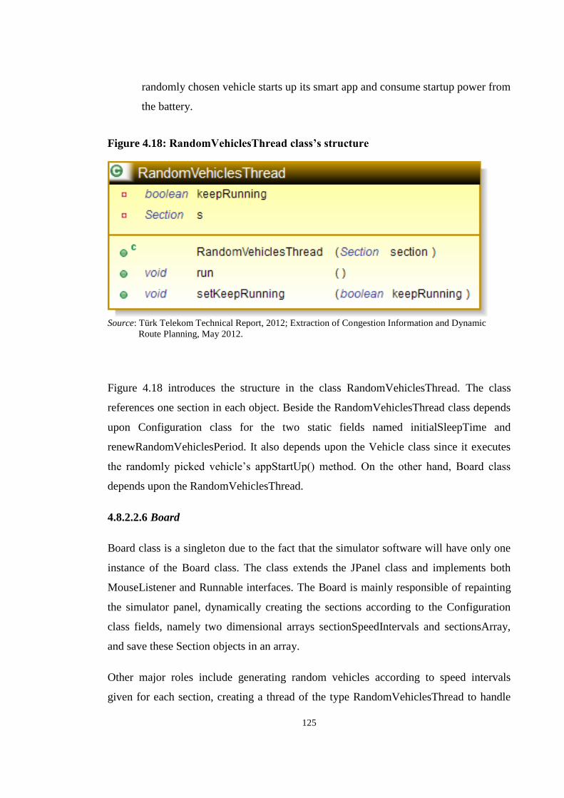
125
randomly chosen vehicle starts up its smart app and consume startup power from
the battery.
Figure 4.18: RandomVehiclesThread class’s structure
Source: Türk Telekom Technical Report, 2012; Extraction of Congestion Information and Dynamic
______ Route Planning, May 2012.
Figure 4.18 introduces the structure in the class RandomVehiclesThread. The class
references one section in each object. Beside the RandomVehiclesThread class depends
upon Configuration class for the two static fields named initialSleepTime and
renewRandomVehiclesPeriod. It also depends upon the Vehicle class since it executes
the randomly picked vehicle’s appStartUp() method. On the other hand, Board class
depends upon the RandomVehiclesThread.
4.8.2.2.6 Board
Board class is a singleton due to the fact that the simulator software will have only one
instance of the Board class. The class extends the JPanel class and implements both
MouseListener and Runnable interfaces. The Board is mainly responsible of repainting
the simulator panel, dynamically creating the sections according to the Configuration
class fields, namely two dimensional arrays sectionSpeedIntervals and sectionsArray,
and save these Section objects in an array.
Other major roles include generating random vehicles according to speed intervals
given for each section, creating a thread of the type RandomVehiclesThread to handle

126
the filling operation on the randomVehiclesArray and the lists contained in
averageSpeedAnalysesArray.
Meanwhile it executes several related operations to perform the tasks defined in the
repaint(Graphics g) method, (i.e. paintComponent(Graphics g), that is called by the
class’s own thread, such as the operational steps to draw section lanes and the texts that
show the average speed calculations, commanding the section objects to calculate and
return the random vehicle array’s average speed, drawing the vehicle images and so on.
Board class extends the JPanel class and implements both Runnable and MouseListener
interfaces. Using the Runnable interface the repaint() method is called to refresh the
graphics components over and over again. The MouseListener interface, on the other
hand, lets the mouse functions to be implemented in the simulator. For example a mouse
function that displays the vehicle information in an information balloon or pop-up
screen when right clicked.
The Board class has 11 fields in total. The fields are explained below:
a. dash1: This field is of the type float. It is used as a global variable and to
determine the array representing dashing pattern in a dashed BasicStroke. This is
used to draw the dashes that limit the width of each lane in both sides and the
vertical borders of each section. It has the value of 10.0f for the float array. It is
called in the final field named “dashed” of the type BasicStroke.
b. dash2: The field acts the same way as dash1 field does. It has the float value of
1.0f for the float array representing the dashing pattern and is used to draw the
green rectangle encloses the vehicles transmitting data. It is called in the final
field named “straight” of the type BasicStroke.
c. dashed: This field is of the type BasicStroke and used as the parameter to set the
stroke of the graphics objects, both for the graphics object that draws the vertical
section borders depicted by the blue dashed lines, and for the graphics object
that draws the hortizontal section lanes depicted by the gray dashed lines.

127
d. straight: This is the same as dashed field except a few different attributes. The
width is 1.0f instead of 2.0f and uses dash2 field as the dashing pattern attribute.
e. instance: This field is a static instance of Board class. It is null at first but then
initialized as a new Board() object in the static method getInstance(). This way
the class is assured to act like a singleton that has a double locking mechanism.
This is due to the fact that the simulator software will have only one instance of
the Board class. The board class is called from outside using the getInstance
method that returns the instance field to the caller.
f. keepRunning: This field is of the type boolean and serves to the purpose of
keeping the thread running or making the thread stop if required (for example in
case the simulator is paused by the user). The thread of the Board class, as
mentioned earlier, refreshes the display screen in the simulator software by
calling the repaint method in each specified time interval.
g. lock: This field is the type of a plain Object. It is used in the getInstance method
to perform the singleton mechanism work. The singleton mechanism has a
synchronized block that uses the lock field to restrict the simultaneous access.
The field is initialized before the object creation at the point it is defined.
h. rnd: The field is of a Random type and is used inside the method
generateRandomVehicles(Section s, int min, int max) while creating the
vehicles. The field determines where to put to image on the display screen. Since
there are lanes and the vehicles need to be located inside these lanes a
calculation in the pixel level is done. The vehicles are located at the pixel 200
plus the randomly chosen lane number times 20 in the y axes. The x axes
coordinate is calculated differently.

128
i. sectionList: The field is of the type ArrayList that takes Section objects in it.
The sections created in the constructor of the Board class are added inside this
statically accessible field.
j. t: This field references a Thread type object. The field is initialized in the Board
constructor using the class itself, e.g. t = new Thread(this), since the class
implements the Runnable interface. The field is started at the last line of the
constructor and is responsible of starting the run() method that executes the
repaint() task.
k. serialVersionUID: The Board class is a serializable and hence it should declare
a static final serialVirsonUID field of type long. It has the value of 1L. The field
is required by default.
The class has neither setter nor getter methods. But it has 12 methods except the
constructor. The details about the methods are given below:
i. Board(): The constructor of the Board has the access type of private. The
constructor makes the screen focusable (coming from JPanel) and sets the
background color to black in the beginning. Right after that, a loop generates as
many sections as the length of the array named sectionsArray declared in
Configuration class. According to the values of the
Configuration.sectionsArray[i][j], the section objects are created. This field of
the Configuration class gives the section parameters that stand for the length and
the number of lanes of each section. Then for each section as many vehicles as it
is specified in Configuration class are created. The vehicles are created with
random speeds where the speed values are between the specified ranges. The
speed ranges are also declared in Configuration class’s sectionSpeedIntervals
field that is a two dimensional array. After the vehicles are created and added
into one section, the RandomVehiclesThread object is created for that section
and its task is started. As the last thing to do, the Board class’s own thread that is

129
responsible of repainting the screen and repeating the calculations is initialized
and started.
ii. Board getInstance(): This method ensures the class is a singleton, in other
words it is initialized using this static method and the it can be initialized only
once from the outside using the static instance field of type Board. The method
implements a double locking mechanism to assure the object creation is done
only once even in multicore systems. The method first of all checks if the private
static field of type Board named instance is null or not. If it is null that means no
instance of the class is created yet. Then the method gets into a synchronized
block to prevent simultaneous access to the line below by multi-threaded
systems. A robust singleton implementation should work in any conditions. This
is why it is needed to ensure it works when multiple threads uses it. Inside the
synchronized block, the instance field is checked to see if it is instantiated, for
the second time. If it is not, then the instance can be instantiated with a new
Board() object and returned in the end.
iii. void generateRandomVehicles(Section s, int min, int max): This method is
responsible of creating as many vehicles as specified by the field
Configuration.numVehiclesPerSection with the random speeds that is in the
range of the parameters min and max. First of all a Battery object with 100
percent energy level and the isConnectedToCharger field set to false. A local
random variable is instantiated. The difference between the min and max values
are calculated in order to generate a random value between zero and the
difference value plus 1. And then this random value is summed up with min
value to be able to set a speed value between min and max parameters for the
vehicle to be created. The vehicle is created at the coordinates; one of which is
defined by Simulation.B_WIDTH minus the half of the startX location of the
section, and the other is defined such that the vehicle image fits in one of the
randomly chosen lanes in the section. The battery object is given as the last
parameter of the vehicle into its constructor. When the vehicle is created, it is
130
ensured that the section given as the first parameter, accepts this vehicle. Lastly
the vehicle’s thread is started that accomplishes the movement task.
iv. void paintComponent(Graphics g): The method acts completely the same way
as paint() method implemented in a JPanel class. It is possible to use the paint()
method instead. The method works whenever the repaint() method is called. The
method clears the screen by calling the super.paintComponent(g). The graphics
parameter “g” is used to draw the components on the JPanel. What the method
does after the cleaning process is that it first of all scans each section in a loop
and calls the method that draws the section and its lanes and gets the average
speed of the section and also draws the value as a string above the section. After
that it gets the average speed for random vehicles that are transmitting their GPS
data and draws it as a string component above the section, as well. Lastly it calls
the method that draws the each vehicle’s images. The method is also responsible
of drawing dashed green lines around the vehicles that are transmitting GPS data
to the server. Further information about the individual vehicles can also be
drawn within this method. Lastly the method synchronizes the default toolkit’s
graphics state and disposes of the graphics context “g” and releases any system
resources that it is using.
v. void drawSectionsAndLanesThenGetAverageSpeed(Graphics g, Section s):
This method draws not only the vertical dashed lines to determine the section
boundaries as well as the horizontal lines that determine the number of lanes in
the section. In addition, it gets the sections average speed and the previous
average speed and assigns these values to its local variables latestAverageSpeed
and currentAverageSpeed of type double, respectively. In case there is no
available average speed data, the method shows the average speed using the
latestAverageSpeed local variable, which is in fact the previous average speed
taken from the section. If nothing is out of order then the average speed is drawn
above the section as a string graphics component. In the following step, the
section color is taken from the section type parameter named “s” using the

131
Section’s getSectionColor(g) method. This method of the Section class not only
returns the suitable section color according to the section’s average speed, but
also draws the congestion weight (an integer value between 1 and 6 such that 1
stands for the heavily congested and 6 stands for the free flow) as a string
graphics component. And then a rectangular area is filled with the color return
from the getSectionColor(g) method via the graphics “g” reference. This colored
rectangular shape is positioned on the simulator screen at an appropriate above
the corresponding section. And then the color of graphics “g” is set to gray and
the required number of lanes is drawn using the dashed lines. Furthermore the
color of “g” is set to blue and then the vertical dashed lines are drawn to indicate
the section borders. In the last line the color of “g” is set back to gray.
vi. void getAverageSpeedForRandomVehicles(Graphics g, Section s): The
method gets the average speed calculation for random vehicles and then draws
the string component to show the value taken for the specific section object. The
drawing operation is done via the Graphics g parameter, and the section
reference is used to determine which section’s average speed for random
vehicles to get and where to draw the string component. After the calculation is
done and the string component is drawn above the appropriate section, lastly for
each vehicle transmitting their GPS data it calls each individual vehicle’s
transmitDataToTheServer() and requestCongestionMap() methods.
vii. void drawVehiclesAndTheirInfo(Graphics g, Section s): At the first step the
stroke type of graphics “g” is set to straight and then the color is set to green.
After that the randomVehiclesArray is copied on a new List<Vehicle> from
section referenced with “s” using the getRandomVehiclesArray() defined in
Section class. And then the image of each vehicle that appear in the section is
drawn in a “for each” loop. After that it is check that if the drawn vehicle is also
contained by the randomVehiclesArray. If it is, then a green rectangular dashed
border is drawn around the image of that vehicle. The vehicle with the green
dashed lines around it means that the vehicle is transmitting at that moment.

132
Lastly when the loop is over, the stroke is set to “dashed” named BasicStroke
type.
viii. void run(): This method must be overridden by the implementing class of the
Runnable interface. It has an infinite while loop that iterates as long as the
keepRunning field is true. It calls the repaint(), then checks if the
Configuration.isWriteToFile field is true, if it is then calls the
executeFileWriting() method. These steps are repeated in each millisecond
defined by repaintFrequencyInMillis static field in the Configuration class.
ix. void executeFileWriting(): The method simply calls the method
writeAverageSpeedAndRandomVehiclesAverageSpeedToFile() for each
specific section in a “for each” loop.
x. void mouseClicked(MouseEvent e): Since the Board class implements the
MouseListener interface it must implement all of the mouse events. When
mouse is clicked this method is called. Its job is to check where the mouse is
clicked and show the info of the clicked vehicle in a box or a pop-up window.
Remaining mouse events defined by void mousePressed(MouseEvent e), void
mouseReleased(MouseEvent e), void mouseEntered(MouseEvent e), void
mouseExited(MouseEvent e) are left empty.
Figure 4.19 depicts the class structure of the Board class. As it can be seen, the Board
class depends upon several other classes. The dependent classes are Configuration,
RandomVehiclesThread, Battery, Vehicle and Simulation. On the other hand the classes
that depend upon the Board are Vehicle and Simulation. Moreover, Board.sectionList
references many Section objects and Board.instance references one Board object.

133
Figure 4.19: The class structure of Board
Source: Türk Telekom Technical Report, 2012; Extraction of Congestion Information and Dynamic
______ Route Planning, May 2012.
4.8.2.2.7 Configuration
The Configuration class is written to define a central access point for the static fields.
Hence the configuration can be handled directly from one generic class. This is why
there are only fields in this class but no methods.
The fields that exist in this class as well as their purposes are given below:
a. BATTERY_THRESHOLD: This field is a static final double and holds the
value that determines the battery threshold. As in battery threshold, it is meant
that the lower limit required to be selected for transmitting data to the server. If

134
the battery energy level is below this constant value then the vehicle that has this
battery is not selected. If it is above this limit, everything works as intended.
b. NUM_VEHICLES_PER_SECTION: It is in fact quite easy to understand
what most of these static final fields stand for, and this field is one of them. It is
basically defining the number of vehicles that must be created in each section
during the initialization of the simulation board. For instance, when the value
assigned to this field is 10, that means there will exist 10n vehicles in total for
the simulation run, where “n” stands for the number of sections. The field is
used by the Board class during the vehicle creation with random attributes.
c. SECTIONS_ARRAY: This field is of type static final integer array with two
dimensions. The first dimension of the array determines the section numbers.
The second dimension has two indexes where the first index determines the
section length and the second index determines the number of lanes in the
section to be created. The field is called in the Board class in the sections
creation process.
d. SECTION_SPEED_INTERVALS: This field is of the type static final integer.
It is a two dimensional array, which the first dimension stands for the section id
and the second dimension stands for the min and max speeds for 0th
and the 1st
indexes, respectively. According to the min and max values defined in the
Configuration, the initial speed values that the vehicles can have in the creation
process are limited in a specific interval for each section. The field is used by the
Board class during the vehicle creation for each section.
e. AVERAGE_SPEED_ANALYSES_ARRAY: It is the field that determines the
number of vehicles to be randomly picked and analyzed. Each index of the array
determines a different number of vehicles that has the proportion of 2:10, 4:10,
6:10, 8:10 to the total number of vehicles defined for each section, i.e.

135
NUM_VEHICLES_PER_SECTION constant. Thus when the value of number
of vehicles per section is 10, the four different set of vehicles will have 2, 4, 6, 8
number of vehicles to be analyzed, respectively. According to length of this
array, constructor of the Section class creates required number of different
arrays. And then the fillRandomVehiclesArray() method fills these arrays with
as many vehicles as these numbers determine.
f. REPAINT_FREQUENCY_IN_MILLIS: This field is of the type static final
int and determined as 30 millisecond in most cases. It is used by the Board class
to find out how frequently to refresh the screen and repaint it. It is done by
sleeping the Board’s thread for the number of milliseconds specified by this
field. The smaller the value the smoother the vehicle motions. The sleep time
also affects the frequency of writing calculated average speeds for each array
into the files.
g. UPDATE_VEHICLE_LOCATION_FREQUENCY: This field is also of the
type static final int. It is used by the Vehicle class. The value of the field affects
the movement frequency of vehicles since it makes the Vehicle thread sleep. In
each iteration the vehicle moves and changes its speed. It is good to assign the
same value as the REPAINT_FREQUENCY_IN_MILLIS constant in order to
avoid the repeating average speed calculations written into the files.
h. INITIAL_SLEEP_TIME: This field is of the type static final long. It is used as
a waiting mechanism in vehicle threads. It gives time to the program to generate
all other vehicles before starting to vehicle movements and related calculations.
It is set as 50 millisecond in most simulation runs.
i. RENEW_RANDOM_VEHICLES_PERIOD: The field is of the type static
final long and is used by the class RandomVehiclesThread. The purpose of this
field is to set the frequency which both the random vehicles array and the

136
random average speed analyses arrays are renewed, in other words filled with
newly selected vehicles, in the run method. Other than filling the random arrays,
the randomly selected vehicles start their applications using the appStartUp()
method. The vehicles with green dashed rectangles around them are identified in
each interval defined by this value, which is in terms of milliseconds. The value
of the constant field is usually 3 seconds in terms of simulation time.
j. CHARGE_FREQUENCY: The field is of the type static final long. It is used
by the Battery class. Since the Battery class is a thread, it has a run method(),
this run method is responsible for the battery charging when the phone is
connected to the charger. The charging operation is done in each cycle of time
defined by this field. Normally the charging operation is done in every 60
seconds for +0.8 percent energy level. However the charge frequency is scaled
into 2000 milliseconds in terms of the simulation time.
k. DECIMAL_FORMAT: This field is of the type static final DecimalFormat. It
defines a decimal format that has a precision up to two digits. This field is used
by the Board class, in both drawSectionsAndLanesThenGetAverageSpeed(…)
method and getAverageSpeedForRandomVehicles(…) method, in order to
format the incoming double values to two digit precision level, or just truncate to
two digits.
l. unlimited: This field is a static boolean type variable. It is used in Vehicle’s
run() method to stop the thread of the vehicles which pass a specific location in
the simulation field. For example in one simulation setup, the vehicles which
were passing the “x coordinates” lesser than -50 were stopped. If it is assigned
with “true” value, then that means the vehicles can move as long as it is
possible, i.e. without a limit on the road.

137
m. isWriteToFile: This field is also of a static boolean type. Its initial value is false
in the simulation setups. Its purpose is to decide whether to write the average
speed results to the files or not. Set true if want the data to be written in the files.
The default value is false. It is used in the run() method of the Board class which
if true executes the method called executeFileWriting().
Figure 4.20: The class structure of Configuration
Source: Türk Telekom Technical Report, 2012; Extraction of Congestion Information and Dynamic
______ Route Planning, May 2012.
Figure 4.20 portrays the class structure modeled for the Configuration class. The class
has no references to other classes. But instead, it has lots of classes which depend on
itself. The depending classes can be listed as RandomVehiclesThread, Vehicle, Section,
Board, and Battery.
4.8.2.2.8 Simulation
The Simulation class extends the JFrame class and is basically responsible of displaying
all the graphical contents of the system within the JFrame. It has two static constant

138
fields B_WIDTH abd B_HEIGHT, as well as a static final long field that determines the
serialVersionUID.
Figure 4.21: The class structure of Simulation
Source: Türk Telekom Technical Report, 2012; Extraction of Congestion Information and Dynamic
______ Route Planning, May 2012.
The class has a main method to launch the application. It simply creates a Simulation
object and sets its visibility to true. The constructor of the class is explained below:
Simulation(): The constructor has no parameters, it is just the default constructor. It
first of all creates a Dimension reference that references to the default toolkit’s screen
size. From there the X and Y screen coordinates where the simulation frame will be
drawn is taken. X coordinate is defined by getting the half of the screen width minus the
half of B_WIDTH constant. The same goes for the Y coordinate, and it is calculated by
getting the screen’s height minus the half of B_HEIGHT constant. And then the default
close operation of the frame is set to EXIT_ON_CLOSE. The title of the simulator is set
as “Smart Transportation Simulator by BAU”. The bounds of the frame is set via the
calculated X and Y integer type coordinates, with a height of B_HEIGHT and a width
of B_WIDTH+20. The frame’s layout is set to BorderLayout(), then an instance is got
using the static method of the Board, namely the Board.getInstance() which instantiates
a Board class object and returns it (it is done this way since the class is a singleton), and
lastly the Board instance is placed in the BorderLayout.Center region.
Figure 4.21 represents the Simulation’s class structure. The Simulation class depends
upon Board class since it adds the Board panel into its center region in the border

139
layout. Likewise, the Board class depends upon Simulation class, as well. Board class
uses the static final fields B_WIDTH and B_HEIGHT that are defined in the Simulation
class. On the other hand, the Section class depends on Simulation class since it uses the
same constant fields defined in Simulation, as well.
4.8.3 CALCULATIONS
All the average speed calculations are performed according to the vehicles generated
randomly using the void generateRandomVehicles(Section s, int min, int max) method. What
the method does is to generate random vehicles for the designated section with speeds
between min and max values. These randomly generated vehicles are put into the
designated section’s vehicle list, to be more precise, into the Section object’s vehicleList
field. Generated vehicles are put into this vehicleList field of type synchronized
ArrayList using the section object’s accept(Vehicle v) method. After each vehicle
creation the vehicle’s thread is started to run. Thus the vehicle starts moving and
changing its speed in every cycle denoted by the updateVehicleLocationFrequency field
in the Configuration class.
The change in the speed of the vehicles leads to varying average speeds for each
section. Board class is responsible for displaying these varying speeds for the sections
and if specified in the Configuration class, writing them into a distinct file for each of
the sections.
4.8.3.1 Average Speed Calculation
As mentioned before, void generateRandomVehicles(Section s, int min, int max) method has
three parameters. The Section s is a reference given to the method as a parameter that
stands for the section to be filled with as many number of randomized vehicles as stated
in numVehiclesPerSection static field of the Configuratiın class. Changing vehicle
speeds in every section causes the average speed in the section to vary in designated
time cycles.
Board class extends JPanel class and implements Runnable class. This means that the
Board class can display the change in average section speeds visually. Thus it should
have a paint(Graphics g) method, or paintComponent(Graphics g) as suggested by the

140
Java gurus. It also should implement the run() method since the class implements the
Runnable interface. The simulator screen can be repainted as frequent as it is specified
by repaintFrequencyInMillis static field in the Configuration class. Everytime the screen
is repainted, the average speed calculations can be performed again to show the change
in the section speed values.
In the method paintComponent(Graphics g), the method that draws the sections and
lanes in the simulator screen, and then gets the average speed values for each section in
the section list is called. The method also does the similar average speed calculations for
the vehicles transmitting their information to the server. The details for this operation
can be found in the next sub-section.
The average speed calculation is done using the well-known averaging method that
simply sums up the vehicle speeds and divides the sum of these speeds to the number of
vehicles present in the vehicle list. This operation is done separately for each section
since the section list is unique for each of them.
4.8.3.2 Randomization Process and Calculations
Randomization process is determined by two factors. One of them is the fact that in
each vehicle location update frequency, the vehicles change their speed, either by
accelerating or decelerating. This process is performed randomly for every vehicle
appearing in the simulator.
On the other hand, the second randomization effect is due to the randomly selected
vehicles among the vehicle list of a section. This randomization process is carried out
by the fillRandomVehiclesArray() method. The method is explained in detail under the
Section class part. Briefly, the method fills the field named randomVehiclesArray which
is of the type synchronized ArrayList in every cycle defined by the
renewRandomVehiclesPeriod in Configuration class. The process is random not only in
terms of determining the number of vehicles to be selected, but also in terms of
determining which individual vehicles among the all vehicles in the section are going to
be selected for transmitting their GPS data to the server. For example, 13 vehicles may
be the random number of vehicles selected in an iteration, whereas 4 vehicles may be

141
the random number of vehicles selected in another iteration. Moreover the vehicle with
the vehicle id of 5 may be selected in an iteration but not in the next iteration, and
instead the vehicle with the vehicle id 17 may be the selected one.
There are also some other ArrayLists that perform the quite similar randomization
process, but this time the number of randomly selected vehicles differ in each such as 20
vehicles, 40 vehicles, 60 vehicles, 80 vehicles out of 100 vehicles in each section. These
random lists are gathered under an ArrayList named averageSpeedAnalysesArray. The
inner lists are the type of synchronized ArrayList objects that have Vehicles in them.
Average speed calculations are performed for all the array lists that are made of
randomly chosen vehicles in every section, as well. The simulation screen shows the
average speed information of each section for randomly determined number of vehicles
which are also randomly selected, in addition to average speed calculated from the
whole vehicle list. The remaining information is written into the files. Thus in the
analyses phase we use all of these outputs to plot and analyze the average speeds.
4.8.4 The Interface
The screenshot in Figure 4.22 that depicts a simulation setup of a single section
roadway with 50 vehicles spread within 5 lanes on-the-go. Each of the vehicle that
appears in the simulation starts from the right hand side of the roadway in a random lane
and drives on the same lane from beginning to the end.
Figure 4.22: The very first look of the simulation environment
Source: Türk Telekom Technical Report, 2012; Extraction of Congestion Information and Dynamic
______ Route Planning, May 2012.

142
Figure 4.23: Snapshot from a newer version of the simulator
Source: Türk Telekom Technical Report, 2012; Extraction of Congestion Information and Dynamic
______ Route Planning, May 2012.
In time, the simulator software has evolved such that it depicts every section divided
with vertical blue dashed lines which is also shown in Figure 4.23. In addition, an
information panel appears for each section that gives the numeric values for the average
speed of all vehicles, another average speed of randomly chosen vehicles, a color bar
that gives an idea about the section speed, and the related congestion weight.
4.8.5 The Analyses
The analyses in this research are done with the data retrieved from various simulation
runs with randomized setups. These simulation setups are classified in two categories
named static random and dynamic random. This section explains what these categories
actually mean, furthermore explains and depicts the several plotted analyses related to
these categories.
4.8.5.1 Static random
In the initial average speed analyses a specific number is set for the number of vehicles
to be randomly chosen, and this number as well as the already chosen vehicles do not
change during the simulation.

143
The simulation runs deployed using such configurations does not reflect a real case.
Because in the real-life, vehicles do not continuously send GPS data to the server. The
mobile application may be closed or run arbitrarily which leads to randomized effects in
terms of simulating such real-life conditions. Hence the number of vehicles as well as
the individual vehicles sending GPS information to the server will keep varying in real-
time.
Three different setups are run in terms of static random analyses. These are 10 vs. 3, 50
vs. 10, and lastly 100 vs. 30. The analyses are performed separately for each section in
the simulation, and for each different setup.
4.8.5.1.1 100 vs. static random 30
Figure 4.24 to Figure 4.27 shows the average speed calculated with 100 vehicles (blue
line) versus the average speed calculated with 30 random vehicles initially chosen (red
line) for each section. The randomly chosen vehicles are static in this analysis. The
speed of the vehicles created in this setup are random values between 1 km/h and 120
km/h. The speed differences between two lines representing the mentioned setup are
lower than 12 km/h. Sometimes the difference is at around 2 km/h. However the
difference may be much greater in consecutive simulation runs with exactly the same
setup since the speed differences between the vehicles can be quite big in such a
configuration. In some other analyses the speed difference between the vehicles of the
same section will be lowered to prevent such unrealistic situations.

144
Figure 4.24: Average speed of 100 vs. static random 30 vehicles for section 1
Source: Türk Telekom Technical Report, 2012; Extraction of Congestion Information and Dynamic
______ Route Planning, May 2012.
Figure 4.25: Average speed of 100 vs. static random 30 vehicles for section 2
Source: Türk Telekom Technical Report, 2012; Extraction of Congestion Information and Dynamic
______ Route Planning, May 2012.
0
10
20
30
40
50
60
70
1 7
13
19
25
31
37
43
49
55
61
67
73
79
85
91
97
10
3
10
9
11
5
12
1
12
7
13
3
13
9
14
5
15
1
15
7
16
3
AV
G S
pe
ed
(km
/h)
AVG Speed Analysis Section 1 - ALL(100) vs RND(30)
All (100) RND (30)
0
10
20
30
40
50
60
70
80
1 7
13
19
25
31
37
43
49
55
61
67
73
79
85
91
97
10
3
10
9
11
5
12
1
12
7
13
3
13
9
14
5
15
1
15
7
16
3
AV
G S
pe
ed
(km
/h)
AVG Speed Analysis Section 2 - ALL(100) vs RND(30)
All (100) RND (30)

145
Figure 4.26: Average speed of 100 vs. static random 30 vehicles for section 3
Source: Türk Telekom Technical Report, 2012; Extraction of Congestion Information and Dynamic
______ Route Planning, May 2012.
Figure 4.27: Average speed of 100 vs. static random 30 vehicles for section 4
Source: Türk Telekom Technical Report, 2012; Extraction of Congestion Information and Dynamic
______ Route Planning, May 2012.
4.8.5.1.2 50 vs. static random 10
From Figure 4.28 to Figure 4.31 another random static analysis is plotted. This time the
analyzed simulation setup is composed of 50 vehicles in each section. The plotting is
done for the average speed of 50 vehicles (blue line) versus average speed of static
0
10
20
30
40
50
60
70
1 7
13
19
25
31
37
43
49
55
61
67
73
79
85
91
97
10
3
10
9
11
5
12
1
12
7
13
3
13
9
14
5
15
1
15
7
16
3
AV
G S
pe
ed
(km
/h)
AVG Speed Analysis Section 3 - ALL(100) vs RND(30)
All (100) RND (30)
0
10
20
30
40
50
60
70
80
1 7
13
19
25
31
37
43
49
55
61
67
73
79
85
91
97
10
3
10
9
11
5
12
1
12
7
13
3
13
9
14
5
15
1
15
7
16
3
AV
G S
pe
ed
(km
/h)
AVG Speed Analysis Section 4 - ALL(100) vs RND(30)
All (100) RND (30)

146
randomly chosen 10 vehicles (red line). In this analysis the difference between the lines
at the same iterations (i.e. time instants) is much bigger. This is due to the fact that the
vehicles in the sections are able to have quite different speed values of between 1 km/h -
120 km/h, and the fact that the randomly chosen vehicles are the ones which move
really slowly compared to the average of all the vehicles. There is another statistical
reason that the randomly chosen vehicles ratio is 1/5, whereas in the previous setup it is
3/10. Hence the difference will be definitely bigger, no matter the average speed of
randomly chosen vehicles is greater or lesser than the average speed of all. The average
speed differences in the sections go beyond 20 km/h and even 30 km/h in some time
instants. Overall, the difference is a lot bigger than the 100 vehicles versus 30 vehicles
case.
Figure 4.28: Comparison of average speed for all 50 vehicles vs. static random 10
vehicles for section 1
Source: Türk Telekom Technical Report, 2012; Extraction of Congestion Information and Dynamic
______ Route Planning, May 2012.
0
20
40
60
80
100
1
28
55
82
10
9
13
6
16
3
19
0
21
7
24
4
27
1
29
8
32
5
35
2
37
9
40
6
43
3
46
0
48
7
51
4
54
1
56
8
59
5
62
2
64
9
67
6
70
3
73
0
75
7
AV
G S
pe
ed
(km
/h)
Iteration Number
AVG Speed Analysis Section 1- ALL(50) vs RND(10)
All (50) RND (10)

147
Figure 4.29: Comparison of average speed for all 50 vehicles vs. static random 10
vehicles for section 2
Source: Türk Telekom Technical Report, 2012; Extraction of Congestion Information and Dynamic
______ Route Planning, May 2012.
Figure 4.30: Comparison of average speed for all 50 vehicles vs. static random 10
vehicles for section 3
Source: Türk Telekom Technical Report, 2012; Extraction of Congestion Information and Dynamic
______ Route Planning, May 2012.
0
10
20
30
40
50
60
701
27
53
79
10
51
31
15
71
83
20
92
35
26
12
87
31
33
39
36
53
91
41
74
43
46
94
95
52
15
47
57
35
99
62
56
51
67
77
03
72
97
55
AV
G S
pe
ed
(km
/h)
AVG Speed Analysis Section 2 - ALL(50) vs RND(10)
All (50) RND (10)
0
20
40
60
80
100
1
28
55
82
10
9
13
6
16
3
19
0
21
7
24
4
27
1
29
8
32
5
35
2
37
9
40
6
43
3
46
0
48
7
51
4
54
1
56
8
59
5
62
2
64
9
67
6
70
3
73
0
75
7
AV
G S
pe
ed
(km
/h)
AVG Speed Analysis Section 3 - ALL(50) vs RND(10)
ALL (50) RND (10)

148
Figure 4.31: Comparison of average speed for all 50 vehicles vs. static random 10
vehicles for section 4
Source: Türk Telekom Technical Report, 2012; Extraction of Congestion Information and Dynamic
______ Route Planning, May 2012.
4.8.5.1.3 10 vs. static random 3
One last analysis in the static random category is carried out by the comparison of 10
vehicles per section versus random statically chosen 3 vehicles. The objective with this
analysis is to test the difference when the ratio between the number of randomly chosen
vehicles and all vehicles is kept the same but the number of the vehicles in a section is
reduced substantially. In other words, the test aims at observing the difference between
“10 vs. 3” and “100 vs. 30” static random vehicles scenarios.
As it can be observed from Figure 4.32 to Figure 4.35, the gap between two average
speed lines become larger compared to the analysis done for 100 vs. 30 static random
vehicles setup.
0
10
20
30
40
50
60
701
27
53
79
10
51
31
15
71
83
20
92
35
26
12
87
31
33
39
36
53
91
41
74
43
46
94
95
52
15
47
57
35
99
62
56
51
67
77
03
72
97
55
AV
G S
pe
ed
(km
/h)
AVG Speed Analysis Section 4 - ALL(50) vs RND(10)
All (50) RND (10)

149
Figure 4.32: Section 1 average speed differences for 10 vs. 3 static random setup
Source: Türk Telekom Technical Report, 2012; Extraction of Congestion Information and Dynamic
______ Route Planning, May 2012.
Figure 4.33: Section 2 average speed differences for 10 vs. 3 static random setup
Source: Türk Telekom Technical Report, 2012; Extraction of Congestion Information and Dynamic
______ Route Planning, May 2012.
0
20
40
60
80
100
1 4 7 10 13 16 19 22 25 28 31 34 37 40 43 46 49 52 55 58 61 64
AV
G S
pe
ed
(km
/h)
Iteration number
Average Speed Analysis for Section 1 - ALL(10) vs. Random Vehicles(3)
All 10
RND 3
0
20
40
60
80
100
1 4 7 10 13 16 19 22 25 28 31 34 37 40 43 46 49 52 55 58 61 64
AV
G S
pe
ed
(km
/h)
Iteration Number
Average Speed Analysis for Section 2 - ALL(10) vs. Random Vehicles(3)
All (10)
RND (3)

150
Figure 4.34: Section 3 average speed differences for 10 vs. 3 static random setup
Source: Türk Telekom Technical Report, 2012; Extraction of Congestion Information and Dynamic
______ Route Planning, May 2012.
The decrease in number obviously causes the difference become larger, hence the error
becomes greater. The average speeds difference is really immense specifically in Figure
4.35 where the minimum difference is 16 km/h, and it even goes up to 40 km/h at some
point.
Figure 4.35: Section 4 average speed differences for 10 vs. 3 static random setup
Source: Türk Telekom Technical Report, 2012; Extraction of Congestion Information and Dynamic
______ Route Planning, May 2012.
0
10
20
30
40
50
60
70
80
1 4 7 10 13 16 19 22 25 28 31 34 37 40 43 46 49 52 55 58 61 64
AV
G S
pe
ed
(km
/h)
Iteration Number
Average Speed Analysis for Section 3 - ALL(10) vs. Random Vehicles(3)
All (10)
RND (3)
0
10
20
30
40
50
60
70
1 4 7 10 13 16 19 22 25 28 31 34 37 40 43 46 49 52 55 58 61 64
AV
G S
pe
ed
(km
/h)
Iteration Number
Average Speed Analysis for Section 4 - ALL(10) vs. Random Vehicles(3)
All (10)
RND (3)

151
4.8.5.2 Dynamic random
This section introduces the dynamic random analyses done in the simulator
development phase. It is called dynamic random or random dynamic in some cases,
since it reflects a dynamic mechanism on the randomization of vehicle selection
process.
The random selections of individual vehicles as well as determination of the random
number of vehicles that are assigned to execute the task of transmitting GPS data
(location, speed and time) to the server are repeated in every specified time interval.
This time interval is defined in the Configuration class with the static field named
renewRandomVehiclesPeriod. Because vehicles that are transmitting GPS data will
keep changing in real-life scenarios. This might happen in some cases where phone
battery is depleted or the user doesn’t want to send the data and/or closes the
application. In the simulator we have taken into account such conditions and hence
implemented the mechanism to renew the random vehicles lists.
The analyses presented in this sub-section reflect more realistic scenarios than the
previous ones thanks to the mechanism that renews the random vehicle lists, which is
the key difference of the random dynamic analyses from the previous analyses. As
mentioned earlier, in the real life scenarios, the vehicles don’t send GPS data
continuously since the smartphone app might be closed arbitrarily by the user or the
phone battery might be low or completely drained. Hence the renewed random vehicles
list provides the same arbitrary conditions occurred in the real life scenarios.
This part of the study includes four different dynamic random analyses for the vehicle
lists in every section. These are 10 vs. dynamic random 10, 20 vs. dynamic random 20,
50 vs. dynamic random 50, and 100 vs. random dynamic 100 vehicles.
4.8.5.2.1 100 vs. random dynamic(100) vehicles
The average speed calculated with 100 vehicles indicated with the blue lines versus the
average speed of the random number of vehicles chosen among this 100 vehicles
indicated by the red lines are plotted in Figure 4.36, Figure 4.37, Figure 4.38 and
Nevertheless, it is still quite obvious to observe the rapid leaps (occurring in a single

152
iteration) at around the iterations mentioned before. This is due to the sudden change in
the random vehicles list at these iterations. Yet, the differences between the real average
speed of the section one and the average speed of the randomly chosen vehicles in the
section one at the same time instant are quite low, namely 3.6 km/h at most. The biggest
average speed difference in the analyses occurs in the second section which is depicted
in Figure 4.37 with and amount of 7 km/h. Briefly, the analyses provide quite
convenient results.
Figure 4.39 for section 1, 2, 3 and 4, respectively.
The random vehicles lists are renewed three times in the analyses generating four
different random vehicles lists in every section. Every new randomization process can
be seen in each figure. For example in Figure 4.36, the renewing processes occur at
around 80th
, 170th
and 270th
iterations. The first section (that is the right most section
and can be observed in Figure 4.36) has relatively closer values of average speeds in
each renewal.
Figure 4.36: Section 1 average speed analysis for 100 vehicles vs. dynamic random
100 vehicles, changing every 2 seconds in terms of simulation time
Source: Türk Telekom Technical Report, 2012; Extraction of Congestion Information and Dynamic
______ Route Planning, May 2012.
50
55
60
65
70
1
13
25
37
49
61
73
85
97
10
9
12
1
13
3
14
5
15
7
16
9
18
1
19
3
20
5
21
7
22
9
24
1
25
3
26
5
27
7
28
9
30
1
31
3
32
5
33
7
AV
G S
pe
ed
(km
/h)
Iteration
Average Speed Analysis for Section 1 - ALL(100) vs. Random Dynamic(100) Vehicles renewing every 2 seconds
All 100 RND Dynamic 100

153
Figure 4.37: Section 2 average speed analysis for 100 vehicles vs. dynamic random
100 vehicles, changing every 2 seconds in terms of simulation time
Source: Türk Telekom Technical Report, 2012; Extraction of Congestion Information and Dynamic
______ Route Planning, May 2012.
Figure 4.38: Section 3 average speed analysis for 100 vehicles vs. dynamic random
100 vehicles, changing every 2 seconds in terms of simulation time
Source: Türk Telekom Technical Report, 2012; Extraction of Congestion Information and Dynamic
______ Route Planning, May 2012.
Nevertheless, it is still quite obvious to observe the rapid leaps (occurring in a single
iteration) at around the iterations mentioned before. This is due to the sudden change in
50
55
60
65
701
13
25
37
49
61
73
85
97
10
9
12
1
13
3
14
5
15
7
16
9
18
1
19
3
20
5
21
7
22
9
24
1
25
3
26
5
27
7
28
9
30
1
31
3
32
5
33
7
AV
G S
pe
ed
(km
/h)
Iteration
Average Speed Analysis for Section 2 - ALL(100) vs. Random Dynamic(100) Vehicles renewing every 2 seconds
All 100 RND Dynamic 100
50
55
60
65
70
1
13
25
37
49
61
73
85
97
10
9
12
1
13
3
14
5
15
7
16
9
18
1
19
3
20
5
21
7
22
9
24
1
25
3
26
5
27
7
28
9
30
1
31
3
32
5
33
7
AV
G S
pe
ed
(km
/h)
Iteration
Average Speed Analysis for Section 3 - ALL(100) vs. Random Dynamic(100) Vehicles renewing every 2 seconds
All 100 RND Dynamic 100

154
the random vehicles list at these iterations. Yet, the differences between the real average
speed of the section one and the average speed of the randomly chosen vehicles in the
section one at the same time instant are quite low, namely 3.6 km/h at most. The biggest
average speed difference in the analyses occurs in the second section which is depicted
in Figure 4.37 with and amount of 7 km/h. Briefly, the analyses provide quite
convenient results.
Figure 4.39: Section 4 average speed analysis for 100 vehicles vs. dynamic random
100 vehicles, changing every 2 seconds in terms of simulation time
Source: Türk Telekom Technical Report, 2012; Extraction of Congestion Information and Dynamic
______ Route Planning, May 2012.
4.8.5.2.2 10 vs. random dynamic(10) vehicles
This analyses aims at observing the big differences between the real average speed and
the random vehicles average speed. Before the analyses it is anticipated that the gap
between the two lines representing the two average speeds shall not be low. The reason
behind the scenes is that the number of vehicles is lowered to 1/10 times of the previous
analysis (containing 100 vehicles). The speed assigned to each vehicle in such a
configuration becomes quite diverse with a high probability and hence the average
speeds generated via the random vehicles list diverge markedly for most of the sections.
50
55
60
65
70
1
13
25
37
49
61
73
85
97
10
9
12
1
13
3
14
5
15
7
16
9
18
1
19
3
20
5
21
7
22
9
24
1
25
3
26
5
27
7
28
9
30
1
31
3
32
5
33
7
AV
G S
pe
ed
(km
/h)
Iteration
Average Speed Analysis for Section 4 - ALL(100) vs. Random Dynamic(100) Vehicles renewing every 2 seconds
All 100 RND Dynamic 100

155
Figure 4.40: Average speed analysis for 10 vehicles vs. dynamic random 10 vehicles
with the renewal time of 2 seconds in Section 1
Source: Türk Telekom Technical Report, 2012; Extraction of Congestion Information and Dynamic
______ Route Planning, May 2012.
Figure 4.41: Average speed analysis for 10 vehicles vs. dynamic random 10 vehicles
with the renewal time of 2 seconds in Section 2
Source: Türk Telekom Technical Report, 2012; Extraction of Congestion Information and Dynamic
______ Route Planning, May 2012.
0
20
40
60
80
1001
13
25
37
49
61
73
85
97
10
9
12
1
13
3
14
5
15
7
16
9
18
1
19
3
20
5
21
7
22
9
24
1
25
3
26
5
27
7
28
9
30
1
31
3
32
5
AV
G S
pe
ed
(km
/h)
Iteration number
Average Speed Analysis for Section 1 - ALL(10) vs. Random Dynamic(10) Vehicles renewing every 2 seconds
All 10 RND Dynamic (10)
0
20
40
60
80
100
1
13
25
37
49
61
73
85
97
10
9
12
1
13
3
14
5
15
7
16
9
18
1
19
3
20
5
21
7
22
9
24
1
25
3
26
5
27
7
28
9
30
1
31
3
32
5
AV
G S
pe
ed
(km
/h)
Iteration number
Average Speed Analysis for Section 2 - ALL(10) vs. Random Dynamic(10) Vehicles renewing every 2 seconds
All 10 RND Dynamic (10)

156
Figure 4.40 is one of the instances that depict the aforementioned situation for the first
section. The randomized vehicle list changes two times in this figure at the iterations of
about 90 and 270, and it is possible to see that at several time instants it yields up to 27
km/h difference from the original values.
The same analysis is plotted in Figure 4.41, Figure 4.42 and Furthermore the difference
values in section 3 plotted by Figure 4.42 changes between 0 to 11 km/h, where as in
Figure 4.43 that plots the last section the difference interval becomes larger to such an
extent that the higher boundary becomes 26 km/h.
Figure 4.43 for section 2, section 3 and section 4, respectively. In section 2 the
difference of the average speeds vary from very low values to some decent ones, where
at some point it becomes 0.1 km/h and at another it becomes 16 km/h.
Figure 4.42: Average speed analysis for 10 vehicles vs. dynamic random 10 vehicles
with the renewal time of 2 seconds in Section 3
Source: Türk Telekom Technical Report, 2012; Extraction of Congestion Information and Dynamic
______ Route Planning, May 2012.
Furthermore the difference values in section 3 plotted by Figure 4.42 changes between 0
to 11 km/h, where as in Figure 4.43 that plots the last section the difference interval
becomes larger to such an extent that the higher boundary becomes 26 km/h.
0
20
40
60
80
100
1
13
25
37
49
61
73
85
97
10
9
12
1
13
3
14
5
15
7
16
9
18
1
19
3
20
5
21
7
22
9
24
1
25
3
26
5
27
7
28
9
30
1
31
3
32
5
AV
G S
pe
ed
(km
/h)
Iteration number
Average Speed Analysis for Section 3 - ALL(10) vs. Random Dynamic(10) Vehicles renewing every 2 seconds
All 10 RND Dynamic (10)

157
Figure 4.43: Average speed analysis for 10 vehicles vs. dynamic random 10 vehicles
with the renewal time of 2 seconds in Section 4
Source: Türk Telekom Technical Report, 2012; Extraction of Congestion Information and Dynamic
______ Route Planning, May 2012.
4.8.5.2.3 20 vs. random dynamic(20) vehicles
This analysis is basically the same as the previous one but just the number of vehicles
starting in each section is doubled, i.e. defined as 20. The plot which is depicted in
Figure 4.44 showed that if it is a lucky random selection, the gap between the lines may
be so lower that it is under even 3 km/h.
For section 2, the same lucky condition is also valid, in other words the difference is
under 3 km/h. But the random selections done in Figure 4.46 and Figure 4.47 are not as
lucky as it was in previous sections.
The observation on Figure 4.46 and Figure 4.47 shows that the average speed variations
are somewhat higher this time. Specifically in Figure 4.46 it is more than 8 km/h and it
gets larger in the following iterations whereas in Figure 4.47 it is above 24 km/h which
constitutes a big difference compared to the first two sections.
0
20
40
60
80
100
1201
13
25
37
49
61
73
85
97
10
9
12
1
13
3
14
5
15
7
16
9
18
1
19
3
20
5
21
7
22
9
24
1
25
3
26
5
27
7
28
9
30
1
31
3
32
5
AV
G S
pe
ed
(km
/h)
Iteration number
Average Speed Analysis for Section 4 - ALL(10) vs. Random Dynamic(10) Vehicles renewing every 2 seconds
All 10 RND Dynamic (10)

158
Figure 4.44: Average speed gaps between 20 vehicles and dynamically selected
random vehicles amongst 20 in section 1
Source: Türk Telekom Technical Report, 2012; Extraction of Congestion Information and Dynamic
______ Route Planning, May 2012.
Figure 4.45: Average speed gaps between 20 vehicles and dynamically selected
random vehicles amongst 20 in section 2
Source: Türk Telekom Technical Report, 2012; Extraction of Congestion Information and Dynamic
______ Route Planning, May 2012.
54
55
56
57
58
59
60
61
62
63
1 4 7 10 13 16 19 22 25 28 31 34 37 40 43 46 49 52 55 58 61
AV
G S
pe
ed
(km
/h)
Iteration number
Average Speed Analysis for Section 1 - ALL(20) vs. Random Dynamic(20) Vehicles renewing every 2 seconds
All 20
RND Dynamic (20)
54
56
58
60
62
64
66
68
1 4 7 10 13 16 19 22 25 28 31 34 37 40 43 46 49 52 55 58 61 64
AV
G S
pe
ed
(km
/h)
Iteration Number
Average Speed Analysis for Section 2 - ALL(20) vs. Random Dynamic(20) Vehicles renewing every 2 seconds
All (20)
RND Dynamic(20)

159
Figure 4.46: Average speed gaps between 20 vehicles and dynamically selected
random vehicles amongst 20 in section 3
Source: Türk Telekom Technical Report, 2012; Extraction of Congestion Information and Dynamic
______ Route Planning, May 2012.
Figure 4.47: Average speed gaps between 20 vehicles and dynamically selected
random vehicles amongst 20 in section 4
Source: Türk Telekom Technical Report, 2012; Extraction of Congestion Information and Dynamic
______ Route Planning, May 2012.
40
45
50
55
60
65
70
1 4 7 10 13 16 19 22 25 28 31 34 37 40 43 46 49 52 55 58 61 64
AV
G S
pe
ed
(km
/h)
Iteration Number
Average Speed Analysis for Section 3 - ALL(20) vs. Random Dynamic(20) Vehicles renewing every 2 seconds
All (20)
RND Dynamic (20)
0
10
20
30
40
50
60
70
1 4 7 10 13 16 19 22 25 28 31 34 37 40 43 46 49 52 55 58 61 64
AV
G S
pe
ed
(km
/h)
Iteration Number
Average Speed Analysis for Section 4 - ALL(20) vs. Random Dynamic(20) Vehicles renewing every 2 seconds
All (20)
RND Dynamic (20)

160
4.8.5.2.4 50 vs. random dynamic(50) vehicles
The analyses done with fifty vehicles in each section provides relatively closer values in
each iteration except in one part of the section 1. Overall, the plots show that an increase
in vehicle numbers leads to the approximations that are closer to real values. The abrupt
leap in the middle part of Figure 4.48 is only because of the large range of assigned
vehicle speeds. In the further analyses the speed range of the vehicles will be narrowed
down greatly to prevent such anomalies.
Figure 4.48: The comparison of 50 vehicles vs. random dynamic 50 vehicles
renewing every 2 seconds in section 1
Source: Türk Telekom Technical Report, 2012; Extraction of Congestion Information and Dynamic
______ Route Planning, May 2012.
The average random vehicles speeds except from the abrupt leap in section 1 converge
in the analyses illustrated by Figure 4.49, Figure 4.50 and Figure 4.51. If the speed
intervals are narrowed down more to accommodate the real-life scenarios, the
simulation results will have no such anomalies.
40
50
60
70
80
90
100
110
120
1
12
23
34
45
56
67
78
89
10
0
11
1
12
2
13
3
14
4
15
5
16
6
17
7
18
8
19
9
21
0
22
1
23
2
24
3
25
4
26
5
27
6
28
7
29
8
AV
G S
pe
ed
(km
/h)
Average Speed Analysis for Section 1 - ALL(50) vs. Random Dynamic(50) Vehicles renewing every 2 seconds
All 50 RND Dynamic (50)
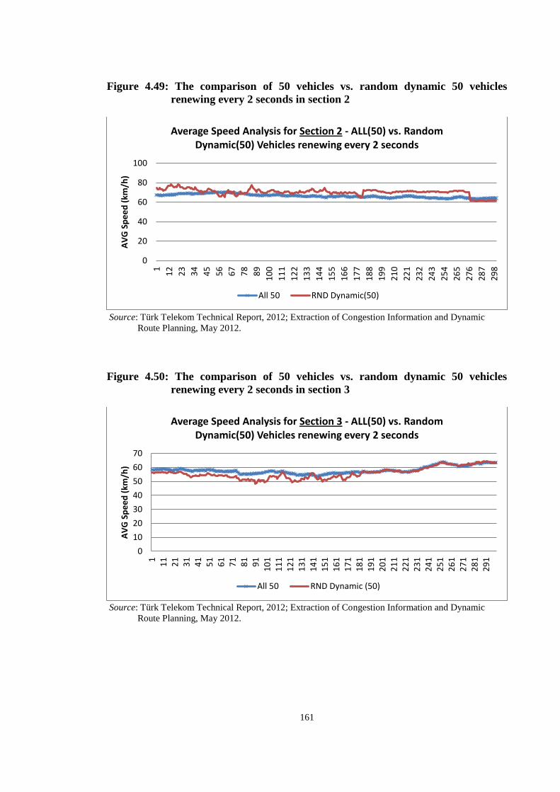
161
Figure 4.49: The comparison of 50 vehicles vs. random dynamic 50 vehicles
renewing every 2 seconds in section 2
Source: Türk Telekom Technical Report, 2012; Extraction of Congestion Information and Dynamic
______ Route Planning, May 2012.
Figure 4.50: The comparison of 50 vehicles vs. random dynamic 50 vehicles
renewing every 2 seconds in section 3
Source: Türk Telekom Technical Report, 2012; Extraction of Congestion Information and Dynamic
______ Route Planning, May 2012.
0
20
40
60
80
1001
12
23
34
45
56
67
78
89
10
0
11
1
12
2
13
3
14
4
15
5
16
6
17
7
18
8
19
9
21
0
22
1
23
2
24
3
25
4
26
5
27
6
28
7
29
8
AV
G S
pe
ed
(km
/h)
Average Speed Analysis for Section 2 - ALL(50) vs. Random Dynamic(50) Vehicles renewing every 2 seconds
All 50 RND Dynamic(50)
0
10
20
30
40
50
60
70
11
12
13
14
15
16
17
18
19
11
01
11
11
21
13
11
41
15
11
61
17
11
81
19
12
01
21
12
21
23
12
41
25
12
61
27
12
81
29
1
AV
G S
pe
ed
(km
/h)
Average Speed Analysis for Section 3 - ALL(50) vs. Random Dynamic(50) Vehicles renewing every 2 seconds
All 50 RND Dynamic (50)

162
Figure 4.51: The comparison of 50 vehicles vs. random dynamic 50 vehicles
renewing every 2 seconds in section 4
Source: Türk Telekom Technical Report, 2012; Extraction of Congestion Information and Dynamic
______ Route Planning, May 2012.
4.8.5.3 Random Dynamic with Multiple Random Lists
This part of the simulator is started in the constructor of the Board class. After the
sections are created, and the vehicles are generated for the section, an instance of the
RandomVehiclesThread class is also created. This class extends the Thread class and is
responsible for the task that fills the randomVehiclesArray, as well as the
averageSpeedAnalysesArray.
While the randomVehiclesArray keeps track of the random number of vehicles selected
among the whole list of vehicles (e.g. 73 vehicles out of 100), the
averageSpeedAnalysesArray keeps track of the 4 other random vehicles lists. These are
namely the lists with i) 1/5 random dynamic vehicles of the whole vehicles in the
section (e.g. 20 vehicles out of 100), ii) 2/5 random dynamic vehicles of the whole
vehicles in the section (e.g. 40 vehicles out of 100), iii) 3/5 random dynamic vehicles of
the whole vehicles in the section (e.g. 60 vehicles out of 100), 4/5 random dynamic
vehicles of the whole vehicles in the section (e.g. 80 vehicles out of 100).
The analyses after this point aims at comparing the outputs generated by 6 different
arrays one of which is the complete vehicle list itself. Other arrays that are plotted in the
0
20
40
60
80
1001
12
23
34
45
56
67
78
89
10
0
11
1
12
2
13
3
14
4
15
5
16
6
17
7
18
8
19
9
21
0
22
1
23
2
24
3
25
4
26
5
27
6
28
7
29
8
AV
G S
pe
ed
(km
/h)
Average Speed Analysis for Section 4 - ALL(50) vs. Random Dynamic(50) Vehicles renewing every 2 seconds
All 50 RND Dynamic (50)

163
following figures are made of by a randomized dynamic array that has random number
of vehicles out of the specified number of total vehicles that are present at the start of
the simulation; for instance, 33 vehicles out of 100 vehicles in a section. The random
number of vehicles to be picked are determined differently in each section.
Nevertheless, every vehicle determined to be picked are different in each section. This
situation reflects the totally random and arbitrary nature of the real-life scenarios.
Furthermore, other randomized dynamic arrays are made of 20, 40, 60 and 80 vehicles
out of 100 vehicles. All of these vehicle lists (i.e. arrays) are illustrated in the same plot
to see the all exact variations in one.
4.8.5.3.1 100 vs. random dynamic (100) and 20, 40, 60, 80 vehicles
Figure 4.52 to Figure 4.55 depicts the all six different outputs at once for each section
respectively. As expected, the most abrupt leaps occur in the lists of both random
dynamic (100) and the dynamic randomly selected 20 vehicles.
Figure 4.52: Average speed analysis for section 1 - all(100) vs. random
dynamic(100), dynamic(20, 40, 60, 80) vehicles renewing every 2
seconds
Source: Türk Telekom Technical Report, 2012; Extraction of Congestion Information and Dynamic
______ Route Planning, May 2012.
45
50
55
60
65
70
75
80
1 2 3 4 5 6 7 8 9 10 11 12 13 14 15 16 17 18 19 20 21 22 23 24 25 26 27 28
AV
G S
pe
ed
(km
/h)
Iteration
All 100RND Dynamic (100)Dynamic 20Dynamic 40Dynamic 60

164
The abnormal leaps observed for the random dynamic (100) is due to the fact that the
number of vehicles to be selected for average speed calculation varies too much. For
example in one selection phase it may be 13, in another it may be 95, and in one last it
may be 55. The picked vehicles are also different in each selection phase. In one
selection only the fastest 10 vehicles may be chosen which results in a high average
speed calculation, whereas in another selection phase the 20 slowest vehicles might be
chosen which results in an opposite condition. Hence the calculations are a highly
unstable for random dynamic (100) list.
Figure 4.53: Average speed analysis for section 2 - all(100) vs. random
dynamic(100), dynamic(20, 40, 60, 80) vehicles renewing every 2
seconds
Source: Türk Telekom Technical Report, 2012; Extraction of Congestion Information and Dynamic
______ Route Planning, May 2012.
35
45
55
65
75
85
95
1 2 3 4 5 6 7 8 9 10 11 12 13 14 15 16 17 18 19 20 21 22 23 24 25 26 27 28
AV
G S
pe
ed
(km
/h)
Iteration
All 100
RND Dynamic (100)
Dynamic(20)
Dynamic(40)
Dynamic(60)
Dynamic(80)

165
On the other hand, the unstable nature of random dynamic 20 is because of the fact that
the ratio is statistically too low. The 20 vehicles chosen randomly might have
completely different speed values, i.e. they might have totally far values from each
other. Thus the average speed calculated using such a list will indicate values far from
acceptable deviation levels. Both of these unsteady conditions are given by all of the
plots in this sub-section.
Figure 4.54: Average speed analysis for section 3 - all(100) vs. random
dynamic(100), dynamic(20, 40, 60, 80) vehicles renewing every 2
seconds
Source: Türk Telekom Technical Report, 2012; Extraction of Congestion Information and Dynamic
______ Route Planning, May 2012.
Moreover another expected result which is based on the idea that the more vehicles
present in a section, the more accurate the average speed calculation results are, is
justified by the Figure 4.52, Figure 4.53, Figure 4.54 and Figure 4.55.
45
50
55
60
65
70
75
1 2 3 4 5 6 7 8 9 10 11 12 13 14 15 16 17 18 19 20 21 22 23 24 25 26 27 28
AV
G S
pe
ed
(km
/h)
Iteration
All 100
RND Dynamic (100)
Dynamic(20)
Dynamic(40)
Dynamic(60)
Dynamic(80)

166
Figure 4.55: Average speed analysis for section 4 - all(100) vs. random
dynamic(100), dynamic(20, 40, 60, 80) vehicles renewing every 2
seconds
Source: Türk Telekom Technical Report, 2012; Extraction of Congestion Information and Dynamic
______ Route Planning, May 2012.
Overall, the closest values to the real average speed are calculated using the random
dynamic 80 vehicles. Second closest values are calculated most of the time by the list
with random dynamic 60 vehicles, later on random dynamic 40, and so on.
4.8.5.3.2 100 vs. random dynamic (100) and 20, 40, 60, 80 vehicles with different
speed intervals constraint in sections
The last analyses carried out during the research are presented in this sub-section. The
purpose in these analyses is to observe the results of the average speed calculation when
speed variation of the vehicles in a section is narrowed down to simulate the real-life
scenarios properly. Because in real-life scenarios there are no such big speed differences
of above 60 km/h or even above 100 km/h.
60
65
70
75
80
85
1 2 3 4 5 6 7 8 9 10 11 12 13 14 15 16 17 18 19 20 21 22 23 24 25 26 27 28
AV
G S
pe
ed
(km
/h)
Iteration
All 100RND Dynamic (100)Dynamic(20)Dynamic(40)Dynamic(60)Dynamic(80)

167
In order to provide the speed intervals at the start of the simulations, each section is
created with the minimum and maximum speed boundaries. Thus the speed of the
vehicles created within a section can only have the values determined between the
minimum and the maximum speed boundaries, at the start of the simulation.
Figure 4.56: Average speed analysis for section 1 implementing the speed intervals
- all(100) vs. random dynamic(100), dynamic(20, 40, 60, 80)
Source: Türk Telekom Technical Report, 2012; Extraction of Congestion Information and Dynamic
______ Route Planning, May 2012.
The simulation outputs presented from Figure 4.56 to Figure 4.59 integrates the section
speed interval constraints. Implementing such a mechanism makes the simulator to be
able to generate closer values to the real average speeds compared to the previous
analyses, even for the random dynamic 20 vehicles list.
55
60
65
70
75
80
85
90
95
100
105
1 2 3 4 5 6 7 8 9 10 11 12 13 14 15 16 17 18 19 20 21 22 23 24 25 26 27 28 29 30
AV
G S
pe
ed
(km
/h)
Iteration
All 100
RND 100
RND Dynamic 20
RND Dynamic 40
RND Dynamic 60
RND Dynamic 80

168
Figure 4.57: Average speed analysis for section 2 implementing the speed intervals
- all(100) vs. random dynamic(100), dynamic(20, 40, 60, 80)
Source: Türk Telekom Technical Report, 2012; Extraction of Congestion Information and Dynamic
______ Route Planning, May 2012.
Figure 4.58: Average speed analysis for section 3 implementing the speed intervals
- all(100) vs. random dynamic(100), dynamic(20, 40, 60, 80)
Source: Türk Telekom Technical Report, 2012; Extraction of Congestion Information and Dynamic
______ Route Planning, May 2012.
40
45
50
55
60
65
70
75
1 2 3 4 5 6 7 8 9 10 11 12 13 14 15 16 17 18 19 20 21 22 23 24 25 26 27 28
AV
G S
pe
ed
(km
/h)
Iteration
All 100
Rnd 100
RND Dynamic 20
RND Dynamic 40
RND Dynamic 60
25
35
45
55
65
75
85
1 2 3 4 5 6 7 8 9 10 11 12 13 14 15 16 17 18 19 20 21 22 23 24 25 26 27
AV
G S
pe
ed
(km
/h)
Iteration
All 100Rnd 100RND Dynamic 20RND Dynamic 40RND Dynamic 60

169
Figure 4.56 illustrates the case for section 1 and has the speed interval starting from 90
km/h to 120 km/h. Figure 4.57 represents the case where the lower speed boundary is 50
km/h and the upper speed boundary is 80 km/h for the second section. Figure 4.58
depicts the third section and has the speed interval between 30 km/h and 50 km/h.
Lastly, Figure 4.59 illustrates the last section and is bounded by the limits of 10 km/h to
30 km/h.
Figure 4.59: Average speed analysis for section 4 implementing the speed intervals
- all(100) vs. random dynamic(100), dynamic(20, 40, 60, 80)
Source: Türk Telekom Technical Report, 2012; Extraction of Congestion Information and Dynamic
______ Route Planning, May 2012.
4.8.6 Traffic Scenarios
Three traffic scenarios are presented in this section using the BAU Traffic Simulator. In
the first scenario the purpose is to simulate an ordinary traffic case. The second scenario
is based on the free flow traffic whereas the third scenario illustrates a traffic accident
with lane closures. All the three scenarios are depicted with various snapshots taken
from the simulator.
15
20
25
30
35
40
45
1 2 3 4 5 6 7 8 9 10 11 12 13 14 15 16 17 18 19 20 21 22 23 24 25 26 27
AV
G S
pe
ed
(km
/h)
Iteration
All 100Rnd 100RND Dynamic 20RND Dynamic 40RND Dynamic 60RND Dynamic 80

170
4.8.6.1 Case 1: Normal Traffic
The scenario shown in Figure 4.60 depicts the traffic simulation setup which has 10
vehicles for each vehicle at the start. The vehicles have the initial speeds specified for
the section in which they are created and located. Moreover, there are 4 sections with
the varying lengths and initial speed intervals. The first section starts from the right
hand side and continues to the left. The vehicles move on the same direction as the
sections, i.e. from right hand side to the left hand side.
In this setup, there are 5 vehicles starting in each section. Section one (the right most
section) has 96 km/h average speed, and the random vehicles average speed that are
transmitting data to the server is 98.67 km/h. The average speed in the first section is
high since its interval is between 90 km/h and 120 km/h. First section’s congestion color
is green and congestion level is 5 which informs that the section is in free flow
condition.
Figure 4.60: Depiction of the first scenario: normal traffic
Source: Türk Telekom Technical Report, 2012; Extraction of Congestion Information and Dynamic
______ Route Planning, May 2012.
In the second section, there are no randomly transmitting vehicles at all. Hence, the
average speed for transmitting vehicles is zero although the real average speed is 88
km/h in this section. The second section’s speed interval is between 50 km/h and 80

171
km/h. The section’s congestion color is green and congestion level is 5 which means
that it is in free flow state.
On the other hand, the third section has an average speed of 25.4 km/h whereas its
average speed for the vehicles that are transmitting GPS data to the central server is
32.67 km/h. The third section’s initial speed interval is 30 km/h for the lower limit and
50 km/h for the upper limit. The section’s congestion color is red and congestion level is
2 which represents its status as congested.
Furthermore, the last section has an initial speed interval between 10 km/h and 30 km/h.
The average speed of all vehicles in the section is 12.4 km/h while the average speed of
the transmitting vehicles is 16.5 km/h. The section’s congestion color is magenta and
congestion level is 1 which notifies that it is heavily/highly congested.
Figure 4.61: Depiction of the same normal traffic scenario showing the
randomization
Source: Türk Telekom Technical Report, 2012; Extraction of Congestion Information and Dynamic
______ Route Planning, May 2012.
The same setup is run again to show the randomization process. This time the
congestion status of each section is as shown in Figure 4.61. In this simulation run, the
first section is highly free (congestion level 6) with 106 km/h average speed and 0 km/h
transmitting vehicles average speed, the second section is in smooth flow (congestion
level 4) with 79.4 km/h average speed and 63 km/h transmitting vehicles average speed,

172
the third section is in dense flow (congestion level 3) with 41.4 km/h average speed and
0 km/h transmitting vehicles average speed, and the last section is in congested state
(congestion level 2) with 25.2 km/h average speed and 6.5 km/h transmitting vehicles
average speed. So the congestion colors are blue, yellow, orange, and red for section 1,
section 2, section 3 and section 4, respectively.
The normal traffic case presented in Figure 4.61 is analyzed in Figure 4.62, Figure 4.63,
Figure 4.64, and Figure 4.65 for section 1, section 2, section 3, and section 4,
respectively. The first section is highly free, around 100-110 km/h as it can be seen in
Figure 4.62 until 15th
iteration (see Appendix A-1: Table 1 for the raw traffic data of
section 1). After that point the fast vehicles get in to the next section and thus the
average speed in section 1 drops considerably, even down to 50 km/h.
Figure 4.62: Average speed analysis for case 1 (normal traffic scenario) in section
1
Source: Türk Telekom Technical Report, 2012; Extraction of Congestion Information and Dynamic
______ Route Planning, May 2012.
The second section has an average speed at around 80 km/h which shows that
congestion status is in smooth flow with an average speed weight of 4 until 13th
iteration, as shown in Figure 4.63. After this point the average speed drops down to 50
40
50
60
70
80
90
100
110
120
1 2 3 4 5 6 7 8 9 10 11 12 13 14 15 16 17 18 19 20 21 22
AV
G S
pe
ed
(km
/h)
Iteration
ALLRND (ALL)Rnd Dynamic (20%)Rnd Dynamic (40%)Rnd Dynamic (60%)Rnd Dynamic (80%)

173
km/h. This is due to the vehicles that have high speed values leave the section and
continue on the next section. Then at 16th
iteration the average speed bursts up to 100
km/h due to entry of many high speed vehicles into the second section.
The third section’s average speed fluctuates between 30 km/h and 40 km/h in the
beginning, which stands for a traffic status of level 3, dense flow. As seen in Figure
4.64, after a while at 13th
iteration, it starts rising due to the high speed vehicles moving
into the section. As more high speed vehicles that come from section 1 and section 2 get
involved in the third section, the average speed increases further. The increase stops
after a while and the average speed gets stabilized between the values of 50 km/h and 70
km/h.
Figure 4.63: Average speed analysis for case 1 (normal traffic scenario) in section
2
Source: Türk Telekom Technical Report, 2012; Extraction of Congestion Information and Dynamic
______ Route Planning, May 2012.
40
50
60
70
80
90
100
110
120
1 3 5 7 9 11 13 15 17 19 21 23 25 27 29 31 33 35 37
AV
G S
pe
ed
(km
/h)
Iteration
ALLRND (ALL)Rnd Dynamic (20%)Rnd Dynamic (40%)Rnd Dynamic (60%)Rnd Dynamic (80%)

174
Figure 4.64: Average speed analysis for case 1 (normal traffic scenario) in section 3
Source: Türk Telekom Technical Report, 2012; Extraction of Congestion Information and Dynamic
______ Route Planning, May 2012.
Figure 4.65: Average speed analysis for case 1 (normal traffic scenario) in section
4
Source: Türk Telekom Technical Report, 2012; Extraction of Congestion Information and Dynamic
______ Route Planning, May 2012.
0
10
20
30
40
50
60
70
80
90
100
1 3 5 7 9 11 13 15 17 19 21 23 25 27 29 31 33 35 37
AV
G S
pe
ed
(km
/h)
Iteration
ALLRND (ALL)Rnd Dynamic (20%)Rnd Dynamic (40%)Rnd Dynamic (60%)Rnd Dynamic (80%)
0
10
20
30
40
50
60
1 3 5 7 9 11 13 15 17 19 21 23 25 27 29 31 33 35 37
AV
G S
pe
ed
(km
/h)
Iteration
ALLRND (ALL)Rnd Dynamic (20%)Rnd Dynamic (40%)Rnd Dynamic (60%)Rnd Dynamic (80%)
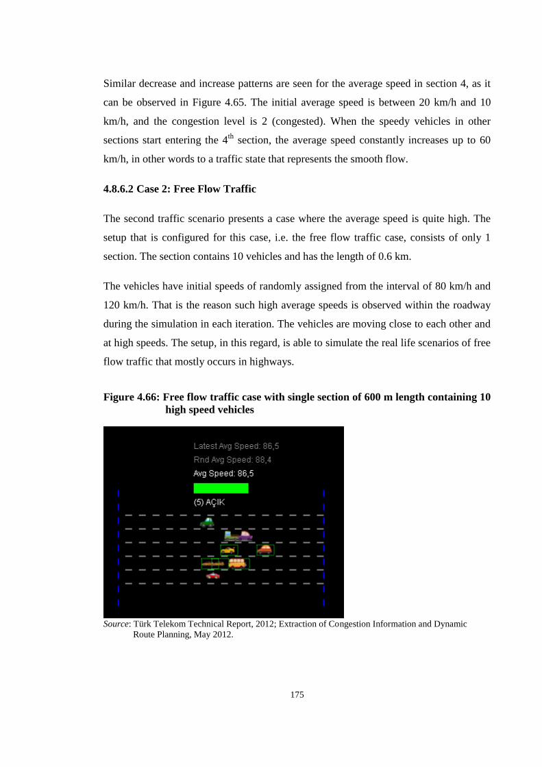
175
Similar decrease and increase patterns are seen for the average speed in section 4, as it
can be observed in Figure 4.65. The initial average speed is between 20 km/h and 10
km/h, and the congestion level is 2 (congested). When the speedy vehicles in other
sections start entering the 4th
section, the average speed constantly increases up to 60
km/h, in other words to a traffic state that represents the smooth flow.
4.8.6.2 Case 2: Free Flow Traffic
The second traffic scenario presents a case where the average speed is quite high. The
setup that is configured for this case, i.e. the free flow traffic case, consists of only 1
section. The section contains 10 vehicles and has the length of 0.6 km.
The vehicles have initial speeds of randomly assigned from the interval of 80 km/h and
120 km/h. That is the reason such high average speeds is observed within the roadway
during the simulation in each iteration. The vehicles are moving close to each other and
at high speeds. The setup, in this regard, is able to simulate the real life scenarios of free
flow traffic that mostly occurs in highways.
Figure 4.66: Free flow traffic case with single section of 600 m length containing 10
high speed vehicles
Source: Türk Telekom Technical Report, 2012; Extraction of Congestion Information and Dynamic
______ Route Planning, May 2012.

176
The snapshot depicted in Figure 4.66 provides the average speed information of the all
vehicles in the section as 86.5 km/h which is also given as “(5) FREE FLOW” in terms
of congestion weight. On the other hand, at the time instant the snapshot is taken, there
appears 5 selected vehicles that are transmitting GPS data to the central system. The
average speed of these transmitting vehicles is 88.4 km/h. The transmitting vehicles, in
this sense, represent close average speed values.
Another free flow traffic case using different parameters is presented in the snapshot
given in Figure 4.67. This setup contains a single section, as well. However, the length
of the single section is 1.6 km. The number of vehicles that appear in the section is 20.
The average speed of the vehicles in the roadway is 87.96 km/h. This average speed
corresponds to the congestion weight “(5) FREE FLOW”, and the congestion color of
green.
Figure 4.67: Free flow traffic with the setup of 20 vehicles in one section of 1600m
length
Source: Türk Telekom Technical Report, 2012; Extraction of Congestion Information and Dynamic
______ Route Planning, May 2012.
On the other hand, the selected vehicles that are transmitting data to the central system
is 10 in the time instant the snapshot is taken. It still keeps varying over time. In such
conditions, the average speed of the transmitting vehicles is 94.42 km/h. The error in

177
this case is higher compared to the previous setup. The approximate error value is ≈7.34
percent. This is due to the increased number of vehicles with varying speeds.
Figure 4.68 depicts the average speed analysis carried out for the setup in Figure 4.67
(see Appendix A-2: Table 1 for the raw traffic data used to represent the free flow case).
The average speed tends to decrease in time due to deceleration of some vehicles even
at times the road traffic is in free flow.
Figure 4.68: Average speed analysis for case 2 (free flow traffic scenario) which
contains 20 vehicles and in a single section
Source: Türk Telekom Technical Report, 2012; Extraction of Congestion Information and Dynamic
______ Route Planning, May 2012.
On the other hand, one other free flow traffic case presented in Figure 4.69 does not
have constantly dropping average speed values for the section as shown in the analysis
given by Figure 4.70, since the vehicles keep traveling at the same speed interval such
as [80,120] km/h. This is a lot more realistic free flow traffic scenario compared to the
previous setup.
80
85
90
95
100
105
110
115
120
1 2 3 4 5 6 7 8 9 10 11 12 13 14 15 16 17 18 19 20 21 22
AV
G S
pe
ed
(km
/h)
Iteration
ALLRND (ALL)Rnd Dynamic (20%)Rnd Dynamic (40%)Rnd Dynamic (60%)Rnd Dynamic (80%)

178
Figure 4.69: Traffic status in a single section for case 2 (free flow traffic scenario)
which contains 20 vehicles with [70,120] km/h speed interval
Source: Türk Telekom Technical Report, 2012; Extraction of Congestion Information and Dynamic
______ Route Planning, May 2012.
Figure 4.70: Average speed analysis for case 2 (free flow traffic scenario) which
contains 20 vehicles and in a single section with [70,120] km/h speed
interval
Source: Türk Telekom Technical Report, 2012; Extraction of Congestion Information and Dynamic
______ Route Planning, May 2012.
75
80
85
90
95
100
105
110
1 2 3 4 5 6 7 8 9 10 11 12 13 14 15 16 17 18 19 20 21 22
AV
G S
pe
ed
(km
/h)
Iteration
ALLRND (ALL)Rnd Dynamic (20%)Rnd Dynamic (40%)Rnd Dynamic (60%)Rnd Dynamic (80%)

179
4.8.6.3 Case 3: Traffic Accident (Multiple Lanes Closed)
The third case simulates the traffic accident scenarios. There are two setups with
different parameters that are simulated in Figure 4.71 and Figure 4.72. Both of the
setups have continuously generated vehicles in them.
The setup depicted in Figure 4.71 is made up of continuously generated vehicles from
the starting section, i.e. the first section at the right hand side. The traffic in the first,
second, and third lanes (in the vertical direction starting from up and going down,
respectively) are highly congested due to the traffic accidents happened in them. The
other lanes, namely the fourth and the fifth, are moving. The movement occurs quite
slowly, though.
Figure 4.71: Traffic accident setup with 42 vehicles in a single section of length 600
meter and 3 closed sections
Source: Türk Telekom Technical Report, 2012; Extraction of Congestion Information and Dynamic
______ Route Planning, May 2012.
There are 27 vehicles which completely stopped in the upper three lanes. Moreover,
there are 15 vehicles which are slowly moving in the lower two lanes. Thus, the system
has 5 lanes and is comprised of 42 vehicles. The length of the section is 600 meters. The
system has an average speed of 3.57 km/h at the time instant the snapshot is taken. The

180
congestion weight is (1) which stands for “HEAVYLY CONGESTED” and the
congestion color is magenta.
At the same time, there are 15 vehicles transmitting their vehicle data amongst the
stopping vehicles in the first three lanes. Hence 15 vehicles out of 26 transmitting
vehicles will report their speed as zero kilometers per hour and their location as constant
coordinates. The average speed of transmitting vehicles, on the other hand, is 4.23 km/h
which is quite close to the real value.
Furthermore, there are 11 vehicles amongst the moving ones in the lower two lanes that
are transmitting their vehicle data to the central server. Hence, only 11 vehicles out of
26 transmitting vehicles will report their speed as non-zero values. The average speed
values calculated for the roadway is low due to the 15 vehicles reporting their speed as
zero.
One other setup is also simulated for the traffic accident case which is depicted in
Figure 4.72. This time the setup contains many more vehicles and two different
sections. The first section at the right hand side has 4 lanes in total. The total number of
vehicles in the section has 32 vehicles. The upper two lanes are heavily congested due
to the traffic accident occurred in the second section (the one at the left hand side).
There are 21 vehicles in the congested lanes and 5 of them are transmitting vehicle data
to the server. These vehicles report their speed as zero km/h and their location as
constant coordinates since they are stopping. On the other hand, the lower two lanes
have 11 vehicles that are moving slowly with approximately 10 km/h speed and only
two of them are reporting their vehicle data to the central structure. The average speed
in in the section to the right hand side (first section) is 3.55 km/h whereas the average
speed reported by the transmitting vehicles is 2.86 km/h. Hence, the reported data has
relatively low error rates. Besides, the congestion weight is again (1) that means
“HEAVYLY/HIGHLY CONGESTED” and the corresponding congestion color is
painted as magenta.

181
Figure 4.72: Traffic accident setup with two sections where two lanes are closed in
each
Source: Türk Telekom Technical Report, 2012; Extraction of Congestion Information and Dynamic
______ Route Planning, May 2012.
The second section (the one on left hand side) is relatively freer in terms of traffic flow.
This is mainly due to the accelerating vehicles in the second section. The traffic
accident occurred before the half distance of the section length, hence there are fewer
vehicles that are stopped compared to the first section. There are 19 vehicles that appear
in the second section where 8 of them are stopped due to the traffic accident in the
upper two lanes. Two of the vehicles among the stopped ones report their data to the
central server. These are reporting zero km/h speed values and are stationary again as
the other crashed vehicles that are mentioned before. On the other hand, only two of the
moving vehicles report their vehicle data.
The average speed of all the vehicles in the section is 5.5 km/h and is marked with the
congestion weight of (1) that stands for “HEAVYLY/HIGHLY CONGESTED” traffic.
On the other hand, the average speed calculated for the vehicles that are reporting data
to the server is 5 km/h. The average speed reported from the transmitting vehicles and
calculated for the all vehicles in the section have a difference of 0.5 km/h which stands
for an error rate of 10 percent.

182
Figure 4.73: The situation before the traffic accident
Source: Türk Telekom Technical Report, 2012; Extraction of Congestion Information and Dynamic
______ Route Planning, May 2012.
Lastly, we represent a traffic accident scenario (case 3) which is comprised of one
section with 4 lanes. The case is visualized by Figure 4.73, Figure 4.74, Figure 4.75 that
show the situation prior to the traffic accident, the situation at the moment the traffic
crash occurs, and the situation when the section starts recovering from crash,
respectively.
Figure 4.74: The situation right after the traffic accident occurs
Source: Türk Telekom Technical Report, 2012; Extraction of Congestion Information and Dynamic
______ Route Planning, May 2012.

183
Figure 4.75: After the crash is cleaned and the lanes are opened to traffic once
again
Source: Türk Telekom Technical Report, 2012; Extraction of Congestion Information and Dynamic
______ Route Planning, May 2012.
Figure 4.76: Average speed analysis for case 3 (traffic accident scenario) which
contains 80 vehicles and two closed lanes in a single section
Source: Türk Telekom Technical Report, 2012; Extraction of Congestion Information and Dynamic
______ Route Planning, May 2012.
30
40
50
60
70
80
90
100
1 3 5 7 9 11 13 15 17 19 21 23 25 27 29 31 33 35 37 39
AV
G S
pe
ed
(km
/h)
Iteration
Average speed analysis for case 3 (traffic accident scenario) which contains 80 vehicles and two closed lanes in a single section
AllRND (ALL)Rnd Dynamic (20)Rnd Dynamic (40)Rnd Dynamic (60)Rnd Dynamic (80)

184
Moreover, the case is analyzed in terms of average speed values in Figure 4.76. There
are 80 vehicles in total in the scenario. The first two lanes (the upper lanes) are closed
due to the crash occurred in the 8th
iteration, as shown in the analyses depicted by
Figure 4.76 (see Appendix A-3: Table 1 for the raw traffic data used to represent the
traffic accident case). The crash causes almost half of the vehicles to stop in a few
seconds. This time corresponds to three iterations as depicted in the analyses. From the
11th
iteration to the 19th
iteration, the upper two of the lanes are unusable because of the
traffic accident. After a while the lanes are opened again, and hence the average speed
of the section starts rising towards 70 km/h. However, it takes a while to fully recover
from the traffic congestion caused by the crash on the upper lanes.

185
5. CONCLUSIONS
In intelligent / smart transportation systems (ITS) applications, it is crucial to provide
and manage the flow of real time information. Corporations which serve their
communication infrastructure for this purpose should consider the dynamic environment
of traffic and also the spatio-temporal features of roads as well as the basic requirements
of the wireless communication such as low latency, reliable transmission and security.
Therefore, powerful communication infrastructure is required to assure optimum
performance for all applications in the ITS field. Processing the large amounts of data
from various types of sources without causing any delay or performance loss is a crucial
task that should be handled by the network provider. However, existing communication
infrastructures should be upgraded for reliable transmission of information by
preventing any kinds of cyber-attacks that may be encountered.
Security of the data should be confirmed by telecom operators especially for the
applications where the timing is critical and the fault tolerance is low such as in
signaling systems in junctions. On the other hand, except the basic features of the
communication network, different properties such as greater processing power and
extensive data storage may be required in specific applications.
Although many projects have been carried out in the different fields of Smart
Transportation; most of them are related with the traffic management. In early ITS
applications; mobility has not been considered as a feature, hence, many applications
that require costly hardware have been developed. On the other hand, in today’s world,
companies give much more attention to the mobility of their products so that different
solutions such as mobile applications and publicly available web sites have been
generated. The major disadvantage of using web-based services for traffic management
is their low accuracy due to the long update time intervals.
For many years, transportation systems relied on infrastructure based equipment such as
loop detectors and cameras. Although the accuracy rate of such systems is high, they
cannot be deployed to the every segment on roads due to their high costs. Hence the
trends in the smart transportation industry have been changed from infrastructure based

186
systems to mobile systems and applications for increasing the reliability while reducing
the cost.
Many applications have been launched to supply real time traffic information to the
drivers but almost all of them have not taken into account of short-term predictions.
Hence, traffic management applications should be developed by considering short-term
predictions about the traffic congestion status on the roads to provide more reliable
route planning features to their customers. The mobility of ITS solutions is considered
as a crucial task in the development of such systems, hence many corporations and
telecom operators have launched their own products based on the user’s mobility.
5.1 PREDICTION SYSTEM CONCLUSIONS
Specifically, in this thesis we first of all surveyed the state of the art in smart
transportation systems in chapter 2. We covered the numerous existing systems in the
literature in great detail which are used in real-life scenarios. We noticed that several of
these systems offered in the literature in order to provide real-time traffic status
solutions and/or an advanced traveler information systems. We classified these systems
in terms of the organization type that offers the solution. In light of this classification
there are 5 different organizational categories. The first category consists of the
solutions offered by top telecom companies such as china mobile, vodafone, verizon,
etc. We provided a comparative table for this category. The second category is named as
the solutions by municipalities. The third category is the solutions by corporations such
as MSN Direct, Pioneer Information Systems, Sigalert, etc. Fourth category includes the
solutions developed by universities. The most prominent university project was carried
out by UC Berkeley called Mobile Millennium. The third and the fourth categories are
given in a table for a brief comparison. Last category introduces the EU projects such as
COOPERS, NOW and HAVEit which aims at providing comprehensive smart
transportation solutions. We saw that although several of these solutions offer beneficial
applications none of them provide a way to predict the short-term future traffic.
Moreover, the research challenges vs. opportunities are reviewed as well as the
communication technologies are discussed. Our studies showed that these technologies
vary in terms of the technology used from conventional approaches to more specified
vehicular communication approaches. We also reviewed literally a large number of

187
simulation tools which were developed to be used in various aspects of Smart
Transportation Systems.
Then we investigated the traffic theory background in detail throughout the chapter 3.
We introduced meaning and the importance of several parameters which are common in
all traffic applications such as density, flow, speed, gap, etc. The basic relationship
between flow, density and velocity is given and its importance is stated. We also
explored the mathematical traffic flow models that are widely mentioned in the traffic
engineering discipline and are listed in two categories, namely Macroscopic and
Microscopic traffic flow models. We described how the traffic flow models are
classified in terms of level of detail, continuity, physical implementation and processes.
We represented both models and their application domain in detail. The fundamental
diagram which is a significant concept that is used in both macroscopic and microscopic
levels of traffic flow is studied, as well. Its parameters and carrying out its calibration
process are presented in great detail. We chose the macroscopic traffic flow models in
our project because of their ability to cope with complex traffic phenomenon with the
use of aggregate traffic variables such as average density, average speed and average
flow. We investigated 4 types of macroscopic models, namely LWR, Payne,
Papageorgiou and CTM. In the end, CTM (Cell Transmission Model) has turned out to
be the most promising and suitable model to proceed with in our project due to its
analytical simplicity, its good style in representing the roadway segments, and ability to
reproduce congestion wave propagation dynamics.
We also described our efforts to construct and introduce a short-term prediction system
in this thesis. We presented a simple yet effective simulation tool called CTMsim and
modeled a portion of TEM freeway ranging from Kavacık to Maslak with it.
Meanwhile, we discussed the rules which need to be considered during the
segmentation process of the roadway. We also described how the colorization process
of the segments is carried out. We mentioned about the several changes done on the tool
and how it allowed us to introduce a mechanism to predict the short-term future traffic
states. We showed our main difference from Berkeley method by introducing the
development of new equations for the travel time calculation. We represented the fact
that the ratio between densities of the successive sections has such an impact that cannot
188
be underestimated on the travel time calculation, as well. Moreover, every component in
the tool's user interface and their functionalities were introduced elaborately in chapter 3
as well as in the video disk provided by the thesis. In addition, we demonstrated two
scenarios modeled in the simulation environment. We depicted a traffic accident
scenario in roadway section number 10 and displayed its effects both visually and
statistically in the area of influence. In addition to the accident scenario, we interpreted
and portrayed the prediction of the traffic state fifteen minute ahead of time in the
second scenario which resulted in a slight difference from the real-time calculation.
All of the tools and their source codes that took place in the development phase as well
as the other resources such as intro video, workshop poster and the presentation
documents are supplied together with this thesis.
5.2 REAL-TIME TRAFFIC SIMULATOR CONCLUSIONS
Traffic management has become a challenging task over years due to the increased
number of vehicles on roads. Many studies have been carried out under the caption of
Intelligent Transportation Systems (ITS), to come up with reliable, efficient and
accurate solutions for traffic congestion that lead to the balanced distribution of vehicles
along the roads according to the road capacities. These studies can be categorized as
infrastructure based and mobile applications according to their data gathering
methodologies. In early ITS systems, infrastructure based, dedicated equipment have
been utilized for data gathering. However, deployment of such systems as data sources
lead to high costs and requires consistent maintenance of equipment to avoid errors and
malfunctions which occur frequently in radars, loop detectors and cameras.
With the recent advances in wireless communications and emergence of sensor-
equipped smartphones, the trends in the smart transportation industry changed from
infrastructure based systems to mobile data gathering devices in order to adapt to the
dynamic environment of traffic and also the spatio-temporal features of roads while
reducing the cost. In chapter 4, new ways of data gathering have been reviewed.
Utilization of these data sources to overcome the limitations of infrastructure based
systems has been introduced. These data sources have been classified as on-board and
189
mobile where former one refers to an embedded hardware deployed on vehicles and the
latter one is based on the utilization of smartphones for data gathering.
Under the caption of on-board data sources, Radio Frequency Identification (RFID)
transponders, License Plate Recognition (LPR) systems, GPS devices have been
investigated and compared according to their benefits and drawbacks. High accuracy
rates that enable the possibility of using on board systems as traffic information probes
to obtain traffic data, have been indicated as the advantage of the utilization of such
systems. On the other hand, common limitations of such systems have been stated as
their high deployment costs and low penetration rates on roads. In order to come up
with a solution for these issues, new approaches based on the utilization of smartphones
in vehicles for data gathering have been introduced. These smartphone based
approaches have been classified as cellular positioning, GPS positioning and hybrid
systems where the former one stands for gathering of location data from triangulation of
cellular network signals, the middle one refers to usage of GPS sensors deployed on
smartphones as a data source and finally the latter one refers to the combination of these
technologies to provide more accurate positioning data while avoiding the battery
drainage arised from GPS based positioning. Based on the comparisons, it has been
concluded that mobile data gathering devices got an edge over others wih their high
accuracy and low cost features, hence state-of-the-art in mobile traffic monitoring
systems has been reviewed.
Extracting the congestion information from the raw data is the essential part of traffic
management systems. However, data extraction phase has solid challenges such as the
determination process of locations that are contained by successive segments. In chapter
4, wireless sensor network based analogy have been proposed to represent the dynamic
nature of traffic and three methods based on dividing road segments into micro-grids
have been proposed to overcome the challenging issues of data extraction. Formulations
and performance results of methods have been presented. Furthermore, improvements
on wireless sensor network analogy have been introduced to overcome issues that
mostly occur when data cannot be obtained from some of the sensors.

190
In addition, the BAU Real Time Traffic Simulator has been introduced in chapter 4 for
analyzing and testing the raw data obtained from our mobile application and
demonstrating the analyses of each method under various real life scenarios. The classes
of BAU Real Time Traffic Simulator and their distinct responsibilities together with
their interaction have been presented throughout chapter 4, as well. Analyses of the
simulation have been categorized into three categories as static, dynamic and multiple
random dynamic analyses where former one requires fixed number of vehicles and
continuous data transmission while latter ones randomize vehicle selection for data
transmission dynamically throughout the simulation. Furthermore, simulation of three
real life scenarios have been conducted to demonstrate our data extraction method
results under normal traffic, free flow and traffic accident with lane closure cases
respectively. The analyses of the simulations of these cases have been presented by
snapshots and average velocity graphics.
The research also covered the investigation of data gathering and extraction
methodologies to develop an accurate and effective dynamic route guidance system
based on alternative route suggestion which plays an essential role on the prevention of
traffic congestion. Dynamic route guidance applications balance the loads on roads by
distributing vehicles based on the road capacities. Alternative routes have been
suggested to the users of such systems for alleviating the congestion on roads. Hence,
development of such systems for providing alternative route suggestions and modeling
traffic conditions and incidents in real time play essential part in traffic management.
Concisely, in this thesis, new technologies for accurate and low cost data gathering have
been investigated. State-of-the-art in smartphone based data acquisition has been
reviewed. New methodologies have been proposed for extracting traffic congestion.
Besides, system architecture and implementation of BAU Real Time Traffic Simulator
have been introduced. Results and analyses of proposed methods have been illustrated
in the simulator, and the use cases of TTraffic have been presented. The simulator
results showed that the traffic status can monitored even when only a small portion of
vehicles report their GPS data over the 3G network in anyway road section.

191
5.3 FUTURE WORK
The future work of the project may include several steps to be carried out. The first step
may examine the validation of the developed prediction method in comparison to the
Berkeley method and the real traffic data provided by IBB Traffic Control Center. It is
expected to attain similar levels of performance for the prediction mechanism using the
real data. Another step may be dedicated to extending the current roadway
configuration, thus it will involve the major arterial roads of the city within the design.
The last step is to carry out a case study of an important intersection in order to apply
adaptive signaling methods using the traffic status results taken from the prediction
mechanism, and hence increase the efficiency of the roads affected by the intersection.
In addition to the possible future work to be done for the prediction mechanism part,
BAU Real-time Traffic simulator can be extended, modified, and improved to provide
more user friendly interface, and ease of access to the configuration parameters.
Specifically a file menu can be added and a comprehensive configuration screen can be
implemented for generating new network setups. The mobile application TTraffic and
the BAU Real-time Traffic Simulator can be fully integrated and the whole system can
be totally automated. Lastly, new methods for the average speed calculations can be
studied using the simulator.
The prediction mechanism gives promising results according to the evaluation of the
system within itself. In other words, our prediction mechanism generates an output
according to the time the user want to predict ahead into the future, and this is compared
with the real traffic status output corresponding to the exact same time of the day the
prediction is given for. Thus the comparison is carried out within the system itself.
However we also need to evaluate the system using the real data that can be provided by
IBB Traffic Control Center. The studies we have done so far will be compared right
after the real data is acquired, and this will undoubtedly generate more satisfactory
results for the verification and calibration phases of our methods.
The prediction system currently models only a tiny portion of the whole traffic system
in the city, namely between Kavacık and Maslak. The system requires the modeling of
remaining arterial roads, namely E5 and TEM, to make it a complete design. Our major
192
goal for this step is to append the remaining arterial roads including the traffic for both
directions. Specifically, we consider of improving the road network in such a way that it
will encompass all the major arterials including both bridges represented just like in the
map supplied by IBB Traffic Control Center. We will need the real data gathered by the
traffic sensors in order to determine the parameters that are used during the
segmentation of the road network and the configuration of each segment within the
network. It is obvious that extending the roadway including the both directions is not a
trivial task. This step will require a decent configuration period, an immense processing
power and optimization processes for proper integration within the design.

193
REFERENCES
Books
Huang, C.-M. & Chen, Y.-S., 2009. Telematics communication technologies and
vehicular networks: wireless architectures and applications. Hershey:
Information Science Publishing.

194
Periodicals
Bar-Gera, H., 2007. Evaluation of a cellular phone-based system for measurements of
traffic speeds and travel times: a case study from Israel. Transportation Research
Part C: Emerging Technologies, 15 (6), pp.380-91.
Bellemans, T., Schutter, B.D. & Moor, B.D., 2003. Models for traffic control. Journal
A, 43 (3-4), pp.13-22.
Caceres, N., Wideberg, J. & Benitez, F., 2008. Review of traffic data estimations
extracted from cellular networks. IET Intelligent Transport Systems Journal, 2
(3), pp.179-92.
Daganzo, C.F., 1993. The Cell Transmission Model Part I: A Simple Dynamic
Representation of Highway Traffic. Transportation Research Part B:
Methodological, 28 (4), pp.269–287.
Dar, K. et al., 2010. Wireless communication technologies for ITS applications [Topics
in Automotive Networking]. IEEE Communications Magazine, 48 (5), pp.156-
162.
Drake, J., Schofer, J. & A.D., M., 1967. A Statistical Analysis of Speed Density
Hypothesis. Highway Research Record, (154), pp.53-87.
Drew, D., 1965. Deterministic Aspects of Freeway Operations and Control. Highway
Research Record, (99), pp.48-58.
Edie, L., 1961. Car-Following and Steady-State Theory for Non-congested Traffic.
Operations Research, (9), pp.66-75.
Fontaine, M.D. & Smith, B.L., 2007. Investigation of the Performance of Wireless
Location Technology-Based Traffic Monitoring Systems. Journal of
Transportation Engineering, 133 (3), pp.157-65.
Gomes, G. & Horowitz, R., 2006. Optimal freeway ramp metering using the asymmetric
cell transmission model. Transportation Research Part C: Emerging
Technologies, 14 (4), pp.244–262.
Greenberg, H., 1959. An Analysis of Traffic Flow. Operations Research, 7 (1), pp.79-
85.
Greenshields, B., 1935. A study of traffic capacity. Highway Research Board
Proceedings, pp.448-77.
Herrera, J. et al., 2010. Evaluation of traffic data obtained via GPS-enabled mobile
phones: the mobile century experiment. Transportation Research Part C, 18 (4),
p.568–583.
Kesting, A. & Reiber, M., 2008. Calibrating car-following models using trajectory data:
Methodological study. Journal of the Transportation Research Board, (2088),
pp.148-56.
Li, B., Yang, Q., Chor, P.L. & Choon, L.G., 2007. A Survey on Mobile WiMAX
[Wireless Broadband Access]. IEEE Communications Magazine, 45 (12), pp.70-
75.
Lighthill, M. & G.B., W., 1955. On Kinematic Waves: II a Theory of Traffic Flow on
Long Crowded Roads. Proceedings of the Royal Society, Series A , pp.317–345.
Lovell, D.J., 2001. Accuracy of speed measurements from cellular phone vehicle
location systems. Journal of Intelligent Transportation Systems, 6 (4), pp.303-25.
Papageorgiou, M., Blosseville, J.M. & Hadj-Salem, H., 1990. Modelling and real-time
control of traffic flow on the southern part of Boulevard Périphérique in Paris,
Part I: Modelling. Transportation Research A, 24A (5), pp. 345-359.

195
Payne, H.J., 1979. FREFLO: A Macroscopic Simulation Model of Freeway Traffic.
Transportation Research Record 722, pp.68-75.
Pipes, L., 1967. Car-Following Models and the Fundamental Diagram of Road Traffic.
Transportation Research, (1), pp.21-29.
Richards, P., 1956. Shock waves on the highway. Operations Research, (4), pp.42–51.
Sohn, K.H.K., 2008. Space-Based Passing Time Estimation on a Freeway Using Cell
Phones as Traffic Probes. IEEE Transactions on Intelligent Transportation
Systems, 9 (3), pp.559-68.
Zhang, H., Ritchie, S.G. & Lo, Z., 2000. Macroscopic modeling of freeway traffic using
an artificial neural network. Transportation Research Record: Journal of the
Transportation Research Board, 1588 (1997), pp.110-19.
Zito, R., D'Este, G. & Taylor, M., 1995. Global positioning systems in the time domain:
how useful a tool for intelligent vehicle-highway systems? Transportation
Research C, 3 (4), pp.193-209.

196
Other Sources
AIMSUN II, n.d. AIMSUN II Traffic Simulator. [Online] Available at:
http://www.aimsun.com/ [Accessed 18 April 2011].
Airsage Inc., 2006. Airsage traffic data server application program interface. Technical
report. University of Virginia, Center for Transportation Studies.
AirSage Inc., 2011. Airsage’s WiSE Technology Overview. [Online] Available at:
http://www.airsage.com/site/index.cfm?id_art=46598&actMenuItemID=21674&v
sprache/EN/AIRSAGE___WiSE_TECHNOLOGY__L.cfm [Accessed 5 May
2011].
ANATOLL, n.d. ANATOLL Traffic Simulator. [Online] Available at:
http://www.compuserve.com [Accessed 11 May 2011].
Anderson, R. et al., 2009. Building a transportation information system using only GPS
and basic SMS infrastructure. In International Conference on Information and
Communication Technologies and Development (ICTD)., 2009, pp. 233-242.
Antoniou, C.R., Balakrishna, H., Koutsopoulos, N. & Ben-Akiva, M.E., 2009. Off-line
and online calibration of dynamic traffic assignment systems. In Proc. 12th IFAC
Symposium on Control in Transportation Systems., 2009,
AT&T and CalTrans District 10, 2007. AT&T puts CalTrans on the road to a better
traffic monitoring system. Case Study. California District 10.
AUTOBAHN, n.d. AUTOBAHN Traffic Simulator. [Online] Available at:
http://www.direktnet.de [Accessed 10 June 2011].
Bertini, R., Lasky, M. & Monsere, C., 2005. Validating predicted rural corridor travel
times from an automated license plate recognition system: Oregon's frontier
project. In Proceedings of the 8th International IEEE Conference on Intelligent
Transportation Systems., 2005, pp. 706-711.
Bolla, R. & Davoli, F., 2000. Road traffic estimation from location tracking data in the
mobile cellular network. In IEEE Wireless Communications and Networking
Conference, (WCNC)., 2000, pp. 1107-1112.
Chadil, N., Russameesawang, A. & Keeratiwintakorn, P., 2008. Real-time tracking
management system using GPS, GPRS and Google earth. In 5th International
Conference on Electrical Engineering/Electronics, Computer,
Telecommunications and Information Technology, ECTI-CON., 2008, pp. 393-
396.
Chang, Y.-M. et al., 2009. Exploring GPS Data for Traffic Status Estimation. In Tenth
International Conference on Mobile Data Management: Systems, Services and
Middleware., 2009, pp. 369-370.
COOPERS, 2006-2010. European Union ITS Project: COOPERS. [Online] Available
at: http://www.cooper-eu.org [Accessed 13 October 2010].
CORSIM, n.d. CORSIM Traffic Simulator. [Online] Available at: http://www.fhwa-
tsis.com [Accessed 21 May 2011].
CVIS, 2004-2010. European Union ITS Project: CVIS. [Online] Available at:
http://www.cvisproject.org/ [Accessed 17 October 2010].
De Fabritiis, C., Ragona, R. & Valenti, G., 2008. Traffic estimation and prediction
based on real time floating car data. In. of the 11th International IEEE Conference
on Intelligent Transportation Systems., 2008, pp. 197–203.

197
DRACULA, n.d. DRACULA Traffic Simulator. [Online] Available at:
http://www.its.leeds.ac.uk/projects/smartest/append3d.html [Accessed 25 May
2011].
FRESIM, n.d. FRESIM Traffic Simulator. [Online] Available at:
http://kuhub.cc.ukans.edu/~pctrans [Accessed 19 April 2011].
Garmin Ltd., 2008a. MSN Direct Receiver/GDB 55 Instructions. [Online] Available at:
http://www8.garmin.com/manuals/MSNDirectReceiver-GDB55_Instructions.pdf
[Accessed 3 January 2011].
Garmin Ltd., 2008b. Garmin nüvi 780 quickstart manual. [Online] Available at:
http://www8.garmin.com/manuals/nuvi780_QuickStartManual.pdf [Accessed 19
February 2011].
Google Maps, n.d. Google Maps Real-time Traffic Status System. [Online] Available at:
https://maps.google.com/ [Accessed 8 November 2010].
Goto, Y., Furusawa, H. & Fukuda, T., 1996. The Melrose Road Traffic Simulation
System. Mitsubishi Denki Kabushiki Kaisha.
Haefner, L.E. & Li, M.S., 1998. Traffic flow simulation for an urban freeway. In
Transportation Conference Proceedings., 1998, pp. 1-6.
HAVEit, 2008-2011. European Union ITS Project: HAVEit. [Online] Available at:
http://www.haveit-eu.org [Accessed 20 December 2010].
Hongsakham W., P.-a.W.P.R., 2008. Estimating road traffic congestion from cellular
handoff information using cell-based neural networks and K-means clustering. In
5th International Conference on Electrical Engineering/Electronics, Computer,
Telecommunications and Information Technology (ECTI-CON)., 2008, pp. 13-16.
Hsiao, W. & Chang, S., 2006. The Optimal Location Update Strategy of Cellular
Network Based Traffic Information System. In IEEE Intelligent Transportation
Systems Conference, ITSC '06., 2006, pp. 248-253.
IBB Traffic, n.d. Istanbul Büyükşehir Belediyesi (IBB) Traffic web interface. [Online]
Available at: http://tkm.ibb.gov.tr/yolDurumu/YogunlukHaritasi.aspx [Accessed 5
October 2010].
IBM Analytics Tool, 2010. IBM & Telvent Smart Traffic Solutions: Predictive Analytics
and Realtime Information. [Online] Available at:
http://www.telvent.com/en/news_center/2010/IBM-and-Telvent-to-Create-
Smarter-Traffic-Solutions-for-Smaller-Cities.cfm [Accessed 28 December 2010].
INTEGRATION, n.d. INTEGRATION Traffic Simulator. [Online] Available at:
http://www.civil.queensu.ca [Accessed 15 March 2011].
Javed, S. et al., 2010. Computational simulation of a macroscopic traffic model for
highways in Pakistan. In 2010 IEEE International Conference on Management of
Innovation and Technology (ICMIT)., 2010, pp. 1182-1187.
Kriegel, H.-P., Renz, M., Schubert, M. & Zuefle, A., 2008. Statistical density prediction
in traffic networks. In Proc. of the 8th SIAM Conference on Data Mining., 2008,
p. 692–703.
KTH Royal Institute of Technology, 2010. IBM Helps City of Stockholm Predict Better
Commuting Options. [Online] Available at: http://www-
03.ibm.com/press/us/en/pressrelease/29903.wss [Accessed 27 2011 April].
Kwon, J., McCullough, B., Petty, K. & Varaiya, P., 2007. Evaluation of PeMS to
Improve the Congestion Monitoring Program. Technical report. Institute of
Transportation Studies, UC Berkeley.

198
Lo, C.-H. et al., 2008. Carweb: A traffic data collection platform. In Proc. of the 9th
International Conference on Mobile Data Management., 2008, p. 221–222.
Lo, C.-H. et al., 2008. CarWeb: A Traffic Data Collection Platform. In The Ninth
International Conference on Mobile Data Management., 2008,
Mathew, T.V., n.d. Microscopic Traffic Flow Modeling. [Online] Department of Civil
Engineering, Indian Institute of Technology Bombay Available at:
http://www.civil.iitb.ac.in/tvm/1100_LnTse/509_lnTse/plain/plain.html [Accessed
10 November 2011].
Menard, T., Miller, J., Nowak, M. & Norris, D., 2011. Comparing the GPS capabilities
of the Samsung Galaxy S, Motorola Droid X, and the Apple iPhone for vehicle
tracking using FreeSim_Mobile. In 14th International IEEE Conference on
Intelligent Transportation Systems (ITSC)., 2011, pp. 985-990.
MICROSIM, n.d. MICROSIM Traffic Simulator. [Online] Available at:
http://www.zpr.uni-koeln.de/~mr/ [Accessed 24 January 2011].
MICSTRAN, n.d. MICSTRAN Traffic Simulator. [Online] Available at:
[email protected] [Accessed 12 April 2011].
Milkovits, M. et al., 2010. DynaMIT 2.0: The Next Generation Real-Time Dynamic
Traffic Assignment System. In Second International Conference on Advances in
System Simulation (SIMUL)., 2010, pp. 45-51.
MITSIM, n.d. MITSIM Traffic Simulator. [Online] Available at:
http://its.mit.edu/products/simlab/ [Accessed 27 March 2011].
MIXIC, n.d. MIXIC Traffic Simulator. [Online] Available at: [email protected] [Accessed
22 February 2011].
Mobile Millennium, 2010. MATLAB implementation of an exact LWR solver. [Online]
UC Berkeley Available at: http://traffic.berkeley.edu/project/downloads/lwrsolver
[Accessed 18 March 2011].
MSN Direct, 2008. MSN Direct Services Architecture. [Online] Available at:
http://msdn.microsoft.com/en-us/library/cc510579.aspx [Accessed 3 December
2010].
Munoz, L. et al., 2004. Methodological calibration of the cell transmission model.
Proceedings of the American Control Conference, 1 , pp.798-803.
Munoz, L. et al., 2003. Traffic density estimation with the cell transmission model.
Proceedings of the American Control Conference 2003, 5 , pp.3750- 3755.
NETSIM, n.d. NETSIM Traffic Simulator. [Online] Available at: http://www-
uftrc.ce.ufl.edu/info-cen/info-cen.htm [Accessed 17 January 2011].
NOW, 2004-2008. European Union ITS Project: NOW. [Online] Available at:
http://www.network-on-wheels.de/ [Accessed 21 November 2010].
PADSIM, n.d. PADSIM Traffic Simulator. [Online] Available at:
http://www.doc.ntu.ac.uk/RTTS [Accessed 21 December 2010].
Paramics, n.d. Paramics Traffic Simulator. [Online] Available at: http://www.paramics-
online.com/ [Accessed 23 July 2011].
Payne, H., 1971. Models of freeway traffic and control. In Mathematical Models of
Public Systems. Simulation Council Proceedings Series., 1971, pp. 51-61.
PeMS, 2010. Performance Measurement System (PeMS) by Caltrans, UC Berkeley, and
PATH. [Online] Available at: https://pems.eecs.berkeley.edu [Accessed 2 May
2011].
Pharos, n.d. Pharos Traffic Simulator. [Online] Available at: [email protected]
[Accessed 19 April 2011].

199
Pioneer, 2010. Pioneer Information Services. [Online] Available at:
http://www.pioneerelectronics.com/PUSA/Car/GPS-Navigation/ [Accessed 16
December 2010].
Plansim-T, n.d. Plansim-T Traffic Simulator. [Online] Available at: http://www.zpr.uni-
koeln.de/GroupBachem/VERKEHR.PG/ [Accessed 11 February 2011].
Poolsawat, A., Pattara-Atikom, W. & Ngamwongwattana, B., 2008. Acquiring road
traffic information through mobile phones. In 8th International Conference on ITS
Telecommunications., 2008, pp. 170-174.
Rahmati, A. et al., 2010. Enabling pervasive mobile applications with the FM radio
broadcast data system. In HotMobile '10 Proceedings of the Eleventh Workshop
on Mobile Computing Systems & Applications., 2010, pp. 78-83.
Sananmongkhonchai, S., Tangamchit, P. & Pongpaibool, P., 2008. Road traffic
estimation from multiple GPS data using incremental weighted update. In Proc. of
the 8th International Conference on ITS Telecommunications., 2008, p. 62–66.
Sanwal, K. & Walrand, J., 1995. Vehicles as probes. Working paper. California PATH,
Institute of Transportation Studies, University of California, Berkeley, CA.
SensorMap, 2008. SenseWeb Project in Microsoft Research. [Online] Available at:
http://www.sensormap.org/sensewebv3/sensormap/ [Accessed 16 February 2011].
Shiva, n.d. Shiva Traffic Simulator. [Online] Available at:
http://www.cs.cmu.edu/~rahuls/shiva.html [Accessed 28 March 2011].
Sigalert, 1998-2012. Lane closure and traffic status monitoring system. [Online]
Available at: http://www.sigalert.com/Map.asp [Accessed 1 March 2011].
SK Telecom, n.d. SK Telecom Nate Drive Telematics service. [Online] Available at:
http://www.sktelecom.com/eng/html/service/Ubiquitous/Telematics.html
[Accessed 8 October 2010].
Terry, D., Thekkath, C. & Zhang, L., 2009. StarTrack System Overview. [Online]
Available at: http://research.microsoft.com/en-us/projects/startrack/ [Accessed 11
February 2011].
THOREAU, n.d. THOREAU Traffic Simulator. [Online] Available at:
[email protected] [Accessed 4 November 2010].
TomTom Inc., 2009. White paper: How TomTom’s HD Traffic and IQ Routes data
provides the very best routing. [Online] Available at:
http://www.tomtom.com/lib/doc/download/HDT_White_Paper.pdf [Accessed 15
October 2011].
Traffic Master, n.d. Traffic Master’s Passive Target Flow Management (PTFM) system.
[Online] Available at: http://trafficmaste.co.uk [Accessed 6 February 2011].
TrafficCast, 2009. TrafficCast White Papers. [Online] Available at:
http://trafficcast.com/white-papers/ [Accessed 17 March 2011].
TrafficCast, 2010. TrafficCast data fusion engine. [Online] Available at:
http://trafficcast.com/technology-platform/data-fusion-engine/ [Accessed 13
January 2011].
Trak.in, 2010. Top 15 Telecom Companies in World. [Online] Available at:
http://trak.in/tags/business/2010/03/31/top-best-telecom-companies-in-world/
[Accessed 1 March 2011].
TranSIMS, n.d. TranSIMS Traffic Simulator. [Online] Available at: http://www-
transims.tssa.lanl.gov/research_team/papers/ [Accessed 7 May 2011].
Treiber, M., 2010. Microsimulation of Road Traffic Flow. [Online] Available at:
http://traffic-simulation.de/ [Accessed 7 February 2011].

200
UC Berkeley, 2008-2011. Mobile Millennium. [Online] Available at:
http://traffic.berkeley.edu/ [Accessed 5 February 2011].
University of Idaho, 2009. Traffic Flow Theory and Concepts. [Online] Available at:
http://www.webs1.uidaho.edu/niatt_labmanual/Chapters/trafficflowtheory/theorya
ndconcepts/ [Accessed 2 December 2011].
VISSIM, n.d. VISSIM Traffic Simulator. [Online] Available at:
http://www.ptv.de/system [Accessed 8 July 2011].
Wang, W. & Mizuta, H., 2008. Probe car based traffic information system experiment
in shenyang. In 8th International Conference on ITS Telecommunications, ITST.,
2008, pp. 334-336.
Wang, P. et al., 2010. Design and implementation of the low-power tracking system
based on GPS-GPRS module. In the 5th IEEE Conference on Industrial
Electronics and Applications (ICIEA)., 2010, pp. 15-17.
Wei, L.-Y., Peng, W.-C., Lin, C.-S. & Jung, C.-H., 2009. Exploring Spatio-Temporal
Features for Traffic Estimation on Road Networks. In ROC., 2009, pp. 1-3.
Westerman, M., Litjens, R. & Linnartz, J.-P., 1996. Integration of probe vehicle and
induction loop data, estimation of travel times and automatic incident detection.
PATH technical report. Institute of Transportation Studies, UC Berkeley.
Work, D., Tossavainen, O.-P., Jacobson, Q. & Bayen, A., 2009. Lagrangian Sensing:
Distributed Traffic Estimation with Mobile Devices. In Proceedings of the 2009
American Control Conference., 2009, pp. 1536-1543.
Wright, J. & Dahlgren, J., 2001. Using vehicles equipped with toll tags as probes for
providing travel times. Working paper. California PATH Program, Institute of
Transportation Studies University of California, Berkeley CA.
Yahoo Maps, n.d. Yahoo Maps Real-time Traffic Flow System. [Online] Available at:
http://maps.yahoo.com/ [Accessed 13 August 2011].
Ygnace, J.-L., Drane, C., Yim, Y. & de Lacvivier, R., 2000. Travel time estimation on
the San Francisco Bay Area network using cellular phones as probes. Working
paper. Institute of Transportation Studies, UC Berkeley, California PATH.
Yim, Y., 2003. The state of cellular probes. Research report. California PATH, Institute
of Transportation Studies, UC Berkeley.
Yim, Y. & Cayford, R., 2001. Investigation of vehicles as probes using global
positioning system and cellular phone tracking: field operational test. Working
paper. California PATH, Institute of Transportation Studies, UC Berkeley.
Yoon, J., Noble, B. & Liu, M., 2007. “Surface street traffic estimation. In Proc. of the
5th International Conference on Mobile Systems, Applications and Services.,
2007, pp. 220–232.
Zeng, X., Tao, C. & Chen, Z., 2009. The application of DSRC technology in Intelligent
Transportation System. In IET International Communication Conference on
Wireless Mobile and Computing (CCWMC)., 2009.

201
APPENDICES

202
Appendix A-1: Table 1. Simulator data for case 1 (normal traffic)
All 20 Vehicles
RND(20) Vehicles
Rnd Dynamic 20% of All
Rnd Dynamic 40% of All
Rnd Dynamic 60% of All
Rnd Dynamic 80% of All
21.8 24 35 15 23.33 31.5
17.8 14.5 31 13 20 23.5
19 8 41 14 23.33 21
27 23.5 40 25 35 30
24.4 18 40 17 34 22.5
26.4 25.5 32 21.5 34.33 25
22 28 22 16 11 16
25.6 26.33 18 12.5 14.33 12.5
20.8 21.33 17 10 12 10
23 28.67 27 14 12.67 14
18 26 30 17 12.67 17
19.6 28.33 33 19.5 15.67 19.5
21 20.33 41 24 24 17
17.6 18.33 34 19.5 19.5 14
16 16 44 22.5 22.5 11.67
15.2 17.33 42 23.5 23.5 8.33
16.2 14 37 24 24 13.67
16.8 15.67 29 24 24 13
15.4 0 16 23 16 19.67
11.8 0 10 9 11.33 10
9.6 0 1 7 10 8.67
10 0 7 1 5.67 9.33
13 0 8 13 8.67 13.67
11.4 0 4 12 10.67 14.67
12.8 0 10 22 11.67 15.67
10 7.67 13 17 12 13
12.6 9.33 24 18 13.67 13.67
17.2 13.67 20 18.5 19.33 16.67
16 11 30 20.5 17.67 16
20.4 16.67 39 21.5 18 15.67
21.2 19.33 50 22 18 16.33
35 6 2 20.5 20.5 14.75
37 8 4 31 31 16.25
37.29 5 1 27.5 27.5 13
52 10.67 5 35.5 35.5 11
52.14 5.33 7 30 30 4.67
52 7.33 4 36 36 10.33
54.71 8.67 2 39.5 39.5 8.67

203
Appendix A-2: Table 1. Simulator data for case 2 (free flow traffic)
All 20 Vehicles
RND(20) Vehicles
Rnd Dynamic 20% of All
Rnd Dynamic 40% of All
Rnd Dynamic 60% of All
Rnd Dynamic 80% of All
95.25 102.25 86.75 91.8 102 102.82
94.3 100 87.25 93.6 99.63 102
93.05 98.5 91.75 87.8 96.63 97.27
93.1 95.5 92 90 92.63 97.64
93.2 94.25 97.75 94.6 93.75 94
91.6 91.5 88.5 92.2 95.25 95.09
89 93.5 83.5 89.2 91.63 92.91
91.5 89.31 98.67 92.5 88.88 93.64
91.05 88.69 96.67 90.5 88 92.64
89.6 87.31 96 87.5 84.13 90.82
88.6 87.54 95 86.88 84.63 89.45
88.45 88.23 96.67 89.25 80.75 88.91
88.35 85.62 92.67 89.25 83.38 90.36
87 0 98.33 83.17 90.67 85.88
85.6 0 92.67 81.5 87.56 84.63
86.8 0 99.33 85 90.11 87.75
88.3 0 104.67 87 90.78 90.25
86.95 0 97 86 89 88.13
89.3 0 98.67 89 87.56 88.38
94.1 98.25 90.25 96.43 95.2 94.55
94.1 98.25 93.25 97.86 94.4 95.64
92.95 93.75 96.25 93.86 95.8 92.82
92.35 93.75 101.25 92.43 96.2 89.09
92.85 93.25 96.75 91.86 94.4 91.18
92 93.75 99 93.57 93.8 88.82
91.3 90 92.5 85.86 91.1 87.55
90.8 92.25 94.75 90.25 89.1 88.67
94.15 96.5 97.25 93.63 91.6 90.11
94.5 95.5 102 95.75 92.8 91.44
94.45 94.08 104.75 95.38 96.5 91
95.2 93.75 104.75 97.5 94.9 92.33
97.65 97.83 111.25 99.5 98.6 93.33
97.3 97.42 112.5 97.5 98.7 94.11
96.35 89.11 102.5 95.83 105.44 102
98.1 94.67 100.5 97.17 104.22 101.18
98.55 99.33 103.5 100.67 105.44 102.73
100.45 100.67 111.75 99.5 106.33 105.73
101.05 101.78 110.25 99.5 110.56 105.27

204
100.8 100 111.75 102.67 111.56 105.55
101.85 103.9 100.25 104.57 105 99.77
104.25 107 107 108.57 107.5 102.85
102 105.3 105.5 103 107.25 101.15
102.05 104.2 107.75 102.14 108 99.85
102.4 104.5 108.25 102.43 105.88 101.31
101.9 105.1 107 101.86 102.63 100.62
100.4 103.2 101.5 99.29 98.13 98.54
98.05 98.91 90.75 87.83 97.88 95.62
94.25 95 86.5 82.5 90.5 89.31
93.75 92.45 93 85.5 90 89.38
95.2 93.36 90 89.5 88.63 91.77
93.5 93.09 87.75 88.5 88.38 89.54
96.7 95.45 92.75 92.83 90.38 91
97.5 98.64 91 84.71 96.64 95.4
97.05 98.07 88.5 86.14 99.82 97.1
96.4 97.14 94 87.14 96.27 97.7
96.85 97.14 94.75 90.86 98.55 96.3

205
Appendix A-3: Table 1. Simulator data for case 3 (traffic accident)
All 80 Vehicles
RND(80) Vehicles
Rnd Dynamic 20% of All
Rnd Dynamic 40% of All
Rnd Dynamic 60% of All
Rnd Dynamic 80% of All
101.06 100.47 98.5 98.13 102.5 101.44
99.65 99.27 102.75 96.75 103.17 99.75
100.18 99.43 98.25 99.25 102.5 102.94
100.58 100.23 98.75 98 103.42 102.25
101.83 101.33 104 97.38 103.75 101.56
101.39 101.4 96.5 100.5 102.83 99.38
101.34 101.5 101.5 99.13 99.27 99.53
100.94 99.83 95.5 100.38 98.45 101.4
83.61 81 85.25 76.5 76.18 83.87
58.69 51.5 70 45.56 50 59.1
49.7 36.5 69 35.75 42.36 53.13
48.76 32.67 71 38.88 42.82 51.93
50.01 55.98 46.75 35.63 87.1 50.13
50.06 56.1 46.75 38 87.4 48.13
50.43 57.17 46.5 36.63 86.2 48.93
51.35 58.57 47.25 38.63 86.4 47.6
51.54 58.02 48.25 39 90.5 48.27
50.51 56.81 43.5 40.75 88.6 46.33
50.91 58.43 43.5 41.63 90.2 48.53
52.58 56.24 4 35.13 32.33 55.64
53.61 56.91 12.25 41.75 35.92 58.57
54.16 57.8 13 43.63 36 61.71
54.34 57.59 14.5 46.63 35.67 59.07
56.69 59.98 10.5 50.25 37.33 59.86
58.24 62.59 14.75 51.5 39.42 63.21
58.2 54.33 60 59.88 55 64.8
59.69 51.11 62.75 65 61.64 66.87
60.29 51 66 65.63 58.82 68.27
60.6 52.56 68.5 65.63 60.55 66.8
61.51 54 64.25 60.63 62.73 67.2
62.71 59.11 68.75 61.75 65.09 68.73
62.7 60.67 43.5 49.13 59.42 76.79
64.16 60.91 49 50.25 64.25 79.21
64.79 61 55.5 51.13 66.33 81.29
64.71 61.28 58.5 52.63 70 80.43
66.33 62.26 57.75 57.13 70.33 81.5
67.23 62.65 59.75 59.13 71.33 81.29
67.63 62.43 57 63.75 70.58 83

206