habilitation thesis: multiscale problems in mechanics of
TRANSCRIPT

Habilitation Thesis:
Multiscale problems in mechanics of materials
Elisa Davoli


Contents
Introduction 1
1 Effective theories for composite materials 15
1.1 Homogenization of integral energies under periodically oscillating differential
constraints . . . . . . . . . . . . . . . . . . . . . . . . . . . . . . . . . . . . . 17
1.2 Multiscale homogenization in Kirchhoff’s nonlinear plate theory . . . . . . . . 77
1.3 Homogenization in BV of a model for layered composites in finite crystal
plasticity . . . . . . . . . . . . . . . . . . . . . . . . . . . . . . . . . . . . . . 127
2 Wulff-shape emergence in crystallization problems 157
2.1 Wulff shape emergence in graphene . . . . . . . . . . . . . . . . . . . . . . . . 159
2.2 Sharp N3/4 law for minimizers of the edge-isoperimetric problem on the tri-
angular lattice . . . . . . . . . . . . . . . . . . . . . . . . . . . . . . . . . . . 193
3 Time-evolving inelastic phenomena 227
3.1 Dynamic perfect plasticity as convex minimization . . . . . . . . . . . . . . . 229
3.2 Dynamic perfect plasticity and damage in viscoelastic solids . . . . . . . . . . 289
Acknowledgements 319


Introduction
A great amount of materials exhibit interesting behaviors, being the result of complex
microstructures, the outcome of involved in-time evolutions, the effect of the action of inter-
nal variables, or the macroscopic counterpart of atomistic interactions. Understanding the
interplay of such different material scales is thus a key problem in materials science. Indeed,
it is crucial for the description of the physics behind phenomena, which are not yet fully
understood, for the development of innovative metamaterials, as well as for the exploration
of their industrial applications.
This habilitation thesis focuses on the analysis of phenomena arising in materials science
and characterized by the presence of multiple scales, with techniques borrowed from the
theory of partial differential equations and from the calculus of variations. The thesis is
subdivided into three chapters, corresponding to three different research directions.
Chapter 1 is concerned with the mathematical description of composite materials, and
with the identification of limiting effective models capturing the macroscopic behavior asso-
ciated with the presence of different kinds of microstructures. I present here a selection of
my papers in this setting.
The first part of Chapter 1 is devoted to a result obtained in [21] in collaboration with
Irene Fonseca (Carnegie Mellon University). Our analysis departs from the observation that
in many applications, in order to establish the macroscopic behavior of a system presenting
a periodic microstructure, we are led to the problem of finding integral representations for
limits as ε goes to zero of oscillating integral energies
uε 7→ˆ
Ω
f(x,
x
εα, uε(x)
)dx,
where Ω ⊂ RN is a bounded open set, and the fields uε are subjected to x -dependent
differential constraints as
N∑
i=1
Ai( xεβ
)∂uε(x)
∂xi→ 0 strongly in W−1,p(Ω;Rl), 1 < p < +∞, (0.1)
1

Introduction
or in divergence form
N∑
i=1
∂
∂xi
(Ai( xεβ
)uε(x)
)→ 0 strongly in W−1,p(Ω;Rl), 1 < p < +∞, (0.2)
with Ai(x) ∈ Ml×d for every x ∈ RN , i = 1, · · · , N , d, l ≥ 1, and where α, β are two
nonnegative parameters.
Oscillating divergence-type constraints as in (0.2) appear in the homogenization theory
of systems of second order elliptic partial differential equations. Indeed, if uε = ∇vε , with
vε ∈ W 1,p(Ω) for every ε > 0, and Ai(x) = A(x) ∈ MN×N for i = 1, · · · , N , then
considering (0.2) reduces to the homogenization problem of finding the effective behavior of
(weak) limits of vε , where
div(A(xε
)∇vε
)→ 0 strongly in W−1,p(Ω), 1 < p < +∞.
These problems have been extensively studied in the literature (see, e.g., [2], [9, Chapter 1,
Section 6], [15], and the references therein).
In the first part of Chapter 1 we present an analysis of the limit case in which α = 0
and β > 0, namely the energy density is independent of the first two variables, and the
fields uε are subject to (0.2). The opposite limit scenario α > 0, β = 0 and (0.1) (i.e., the
energy density is oscillating but the differential constraint is fixed and in “non-divergence”
form) is the subject of [22] (see also [23]). In particular, we analize the setting in which the
coefficients Ai are nonconstant L∞ -maps, Ai ∈ L∞(RN ;Ml×d) for every i = 1, . . . , N , the
energies under consideration are of the type
uε 7→ˆ
Ω
f(uε(x)) dx,
where the energy density f satisfies standard p-growth assumptions, uε u weakly in
Lp(Ω;Rd), and
A divε uε :=
N∑
i=1
∂
∂xi
(Ai(xε
)uε(x)
)→ 0 strongly in W−1,q(Ω;Rl)
for all 1 ≤ q < p . Our analysis includes the case when q = p if the coefficients Ai
are smooth. However, in the general situation when the maps Ai are only bounded, the
assumption 1 ≤ q < p is required, in order to satisfy some truncation and p -equiintegrability
arguments. Our main results are a characterization of the limiting homogenized energy and
the observation that, as opposed to the case in which the operators Ai are constant, the
homogenized energy FA might not, in principle, be local, i.e., we can not expect that there
exists fhom : Ω× Rd → [0,+∞) such that
FA (u) =
ˆ
Ω
fhom(x, u(x)) dx. (0.3)
We provide, in fact, an explicit example showing that locality in the sense of (0.3) may fail
2

Introduction
even when the function f is convex in its second variable.
The second part of Chapter 1 focuses on the problem of identifying lower dimensional
models describing thin three-dimensional structures. This is a classical question in mechanics
of materials, which, since the early ’90s, has been studied successfully by means of variational
techniques. In particular, starting from the seminal papers [1, 29, 30, 32] hierarchies of
limiting models have been deduced by Γ-convergence, depending on the scaling of the elastic
energy with respect to the thickness parameter.
The first homogenization results in nonlinear elasticity have been proved in [10] and [37].
In these two papers, A. Braides and S. Muller assume p -growth of a stored energy density
W that oscillates periodically in the in-plane direction. They show that, as the periodicity
scale goes to zero, the elastic energy converges to a homogenized integral functional whose
density is obtained by means of an infinite-cell homogenization formula.
In [7, 11] the authors treat simultaneously homogenization and dimension reduction for
thin plates, in the membrane regime and under p-growth assumptions of the stored energy
density. More recently, in [31], [38], and [44] models for homogenized plates have been
derived under physical growth conditions for the energy density.
In the second part of Chapter 1 we present a multiscale version of the results in [31]
and [44]. Let
Ωh := ω ×(−h2 , h2
)
be the reference configuration of a nonlinearly elastic thin plate, where ω is a bounded
domain in R2 , and h > 0 is the thickness parameter. We assume that the plate undergoes
the action of two in-plane homogeneity scales: a coarser one, henceforth denoted by ε(h),
and a finer one, ε2(h), where h and ε(h) are monotone decreasing sequences of positive
numbers, h→ 0 and ε(h)→ 0 as h→ 0. The rescaled nonlinear elastic energy is given by
J h(v) :=1
h
ˆ
Ωh
W
(x′
ε(h),x′
ε2(h),∇v(x)
)dx
for every deformation v ∈ W 1,2(Ωh;R3), where the stored energy density W is periodic in
its first two arguments and satisfies classical assumptions in nonlinear elasticity, as well as a
nondegeneracy condition in a neighborhood of the set of proper rotations (see [31, 38, 44]).
We focus on the scaling of the energy which corresponds to Kirchhoff’s plate theory, and we
consider sequences of deformations vh ⊂W 1,2(Ωh;R3) verifying
lim suph→0
J h(vh)
h2< +∞. (0.4)
The main result of this section, proved in [12] jointly with Laura Bufford (former PhD-
student at Carnegie Mellon University) and Irene Fonseca, is an identification of the effec-
tive energies arising as limiting descriptions of the rescaled elastic energiesJ h(vh)
h2
, and
depending on the interaction of the two homogeneity scales with the thickness parameter.
The main difference with respect to [31] and [44] is in the structure of the homogenized
energy densities, which are obtained by means of a double pointwise minimization, first with
3

Introduction
respect to the faster periodicity scale, and then with respect to the slower one, and to the
x3 variable.
The third and last part of Chapter 1 is devoted to the mathematical modeling of meta-
materials. These are artificially engineered composites whose heterogeneities are optimized
in order to improve structural performances. Due to their special mechanical properties,
arising as a result of complex microstructures, metamaterials play a key role in industrial
applications and are an increasingly active field of research. Two natural questions when
dealing with composite materials are how the effective material response is influenced by
the geometric distribution of its components, and how the mechanical properties of the
components impact the overall macroscopic behavior of the metamaterial.
In the result presented in this last part of Chapter 1 (and obtained jointly with Carolin
Kreisbeck (University of Utrecht) and Rita Ferreira (KAUST) in [20]), we investigate these
questions for a special class of metamaterials with two characteristic features that are of
relevance in a number of applications: (i) the material consists of two components arranged
in a highly anisotropic way into periodically alternating layers, and (ii) the (elasto)plastic
properties of the two components exhibit strong differences, in the sense that one is rigid,
while the other one is considerably softer, thus allowing for large (elasto)plastic deformations.
The analysis of variational models for such layered high-contrast materials was initiated
in [13]. There, the authors derive a macroscopic description for a two-dimensional model
in the context of geometrically nonlinear but rigid elasticity, assuming that the softer com-
ponent can be deformed along a single active slip system with linear self-hardening. These
results have been extended to general dimensions, to energy densities with p -growth for
1 < p < +∞ , and to the case with non-trivial elastic energies, which allows treating very
stiff (but not necessarily rigid) layers, see [14].
In the third part of Chapter 1 we carry the ideas of [13] forward to a model for
plastic composites without linear hardening, in the spirit of [18], and we study the effective
behavior of a two-dimensional variational model within finite crystal plasticity for high-
contrast bilayered composites. Precisely, we consider materials arranged into periodically
alternating thin horizontal strips of an elastically rigid component and a softer one with one
active slip system. The energies arising from these modeling assumptions are of integral
form, featuring linear growth and non-convex differential constraints. This change turns the
variational problem in [13], having quadratic growth (cf. also [16, 17]), into one with energy
densities that grow merely linearly.
The main novelty lies in the fact that the homogenization analysis must be performed
in the class BV of functions of bounded variation (see [4]) to account for concentration
phenomena. This gives rise to conceptual mathematical difficulties: on the one hand, the
standard convolution techniques commonly used for density arguments in BV or SBV can-
not be directly applied because they do not preserve the intrinsic constraints of the problem;
on the other hand, constraint-preserving approximations in this weaker setting of BV are
rather challenging, as one needs to simultaneously regularize the absolutely continuous part
of the distributional derivative of the functions and accommodate their jump sets. A crucial
first step in the asymptotic analysis is the characterization of rigidity properties of limits of
4

Introduction
admissible deformations in the space BV of functions of bounded variation. In particular,
we prove that, under suitable assumptions, the two-dimensional body may split horizontally
into finitely many pieces, each of which undergoes shear deformation and global rotation.
This allows us to identify a potential candidate for the homogenized limit energy, which we
show to be a lower bound on the Γ-limit. Our main result is to show, in the framework
of non-simple materials, a complete Γ-convergence analysis, including an explicit homoge-
nization formula, for a regularized model with an anisotropic penalization in the in-layer
direction.
Chapter 2 of the thesis focuses on the emergence of Wulff shapes in crystallization
problems. The content of Chapter 2 is the subject of [24] and [25], and is based on a
collaboration with Paolo Piovano (University of Vienna) and Ulisse Stefanelli (University of
Vienna).
In the last decades an increasing interest has arisen for carbon-based materials, such as
carbon nanotubes, fullerenes and ultra-thin graphite films, due to their unexpected electro-
magnetic properties, e.g., superconductivity and anomalous quantum Hall effects. One of
the most promising materials (investigated among others by the Nobel prizes Geim and
Novoselov) is graphene, which can be seen as the basic constituent of more complex carbon-
based structures. This material ideally corresponds to a regular, two-dimensional layer of
carbon atoms. Each atom is covalently bonded to three neighbors. These covalent bonds are
of sp2 -hybridized type and ideally form 2π/3 angles in a plane, so that graphene patches
can be identified as subsets of an infinite hexagonal lattice.
In order to describe these bonds, some phenomenological interaction energies (including
two- and three-body interaction terms) have been presented and partially validated. The ar-
rangement of carbon atoms in the two-dimensional crystal emerges then as the global effect
of the combination of local atomic interactions, and can be seen as the result of a geometric
optimization process: by identifying the configuration of n carbon atoms with their positions
x1, . . . , xn ⊂ R2 , one minimizes a given configurational energy E : R2n → R ∪ ∞ and
proves that the minimizers are indeed subsets of a regular hexagonal lattice. The configura-
tional energies for carbon feature a decomposition E = E2 + E3 where E2 corresponds to
an attractive-repulsive two-body interaction, favouring some preferred spacing of the atoms,
and E3 encodes three-body interactions, expressing the specific geometry of sp2 covalent
bonding in carbon.
The above variational viewpoint brings the study of graphene geometries into the realm of
the so-called crystallization problems. In the hexagonal setting, the crystallization problem
for a finite number of carbon atoms is studied in [35] where the periodicity of ground states
as well as the exact quantification of the ground-state energy is obtained.
In the first part of Chapter 2 we present an equivalent characterization of graphene
flakes as particle configurations maximizing a discrete “area” and minimizing a discrete
“perimeter”. Our analysis moves from the consideration that, as the configurational energy
favors bonding, ground states are expected to have minimal perimeter, since boundary
atoms have necessarily less neighbors. This heuristics is here made precise by providing a
5

Introduction
new identification of ground states based on a crystalline isoperimetric inequality. Indeed,
we prove that ground states correspond to isoperimetric extremizers and we determine the
exact isoperimetric constant. Analogous results had been obtained in [33, 34] for the square
lattice. As a byproduct of our isoperimetric characterization we are able to investigate the
edge geometry of graphene patches. Graphene atoms tend to naturally arrange themselves
into hexagonal samples whose edges can have, roughly speaking, two shapes: they can
either form zigzag or armchair structures. We prove here that hexagonal configurations
having armchair edges do not satisfy the isoperimetric equality, whereas those with zigzag
edges do.
The minimality of the ground-state perimeter gives rise to the emergence of large poly-
gonal clusters as the number of atoms n increases. Indeed, one is interested in identifying
a so-called Wulff shape to which all properly rescaled ground states converge. This had
been successfully obtained for both the triangular [6, 39] and the square lattice [33, 34]
beforehand, showing that ground states approach a hexagon and a square, respectively, as
n → ∞ . Quite remarkably, in both the triangular and the square case it has been proved
that ground states differ from the Wulff shape by at most O(n3/4) atoms, this bound being
sharp. This is what is usually referred to as the n3/4 -law.
Relying on our novel discrete isoperimetric inequality, our main result is an analysis
of the asymptotic behavior of graphene patches as the number of particles grows, proving
their convergence to a limit macroscopic hexagonal Wulff shape. In particular, ground
states with n atoms in two dimensional graphene sheets are shown to deviate from suitable
hexagonal configurations with zigzag edges and from a limit hexagonal Wulff shape by at
most Khn3/4 + o(n3/4) particles. The constant Kh is explicitly computed and proved to be
sharp.
A parallel analysis in the triangular lattice is presented in [25] and in the second part
of Chapter 2, allowing to provide a characterization of minimizers of the so-called “edge-
isoperimetric” problem, which plays a key role in the variational description of many classi-
fications and clustering tasks. Extremizers of the edge-isoperimetric problem are shown to
deviate from suitable hexagonal configurations in the triangular lattice and from the Wulff
shape by at most Ktn3/4 + o(n3/4) particles. Our result provides a new, alternative proof
of the n3/4 -law in the triangular lattice. As a by-product of our analysis an explicit sharp
value for Kt is also identified.
Our estimates in the triangular and hexagonal lattice provide a measure in different
topologies of the fluctuation of the isoperimetric configurations with respect to suitable
hexagonal configurations.
The mathematical modeling of inelastic phenomena is a very active research area, at the
triple point between mathematics, physics, and materials science. Chapter 3 is devoted to
two results related to the modeling of inelastic phenomena in a dynamic setting.
In the first part of Chapter 3 we discuss a new approximation result for solutions to
6
Introduction
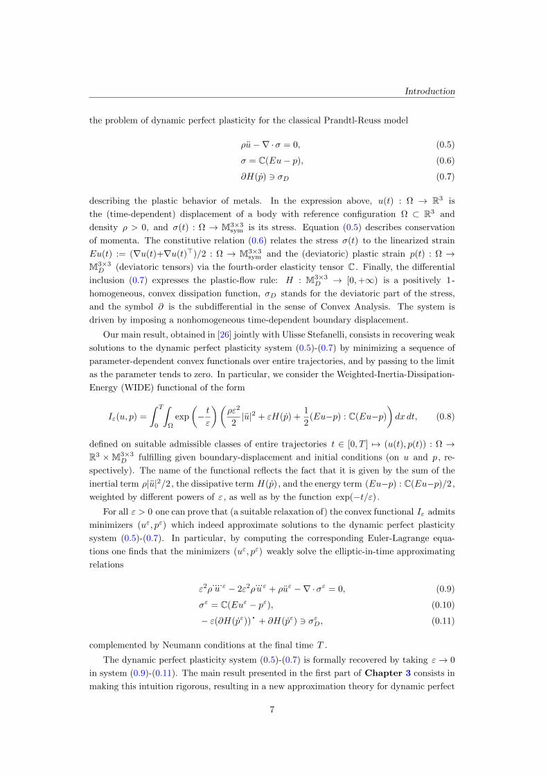
the problem of dynamic perfect plasticity for the classical Prandtl-Reuss model
ρu−∇ ·σ = 0, (0.5)
σ = C(Eu− p), (0.6)
∂H(p) 3 σD (0.7)
describing the plastic behavior of metals. In the expression above, u(t) : Ω → R3 is
the (time-dependent) displacement of a body with reference configuration Ω ⊂ R3 and
density ρ > 0, and σ(t) : Ω → M3×3sym is its stress. Equation (0.5) describes conservation
of momenta. The constitutive relation (0.6) relates the stress σ(t) to the linearized strain
Eu(t) := (∇u(t)+∇u(t)>)/2 : Ω → M3×3sym and the (deviatoric) plastic strain p(t) : Ω →
M3×3D (deviatoric tensors) via the fourth-order elasticity tensor C . Finally, the differential
inclusion (0.7) expresses the plastic-flow rule: H : M3×3D → [0,+∞) is a positively 1-
homogeneous, convex dissipation function, σD stands for the deviatoric part of the stress,
and the symbol ∂ is the subdifferential in the sense of Convex Analysis. The system is
driven by imposing a nonhomogeneous time-dependent boundary displacement.
Our main result, obtained in [26] jointly with Ulisse Stefanelli, consists in recovering weak
solutions to the dynamic perfect plasticity system (0.5)-(0.7) by minimizing a sequence of
parameter-dependent convex functionals over entire trajectories, and by passing to the limit
as the parameter tends to zero. In particular, we consider the Weighted-Inertia-Dissipation-
Energy (WIDE) functional of the form
Iε(u, p) =
ˆ T
0
ˆ
Ω
exp
(− tε
)(ρε2
2|u|2 + εH(p) +
1
2(Eu−p) : C(Eu−p)
)dx dt, (0.8)
defined on suitable admissible classes of entire trajectories t ∈ [0, T ] 7→ (u(t), p(t)) : Ω →R3 ×M3×3
D fulfilling given boundary-displacement and initial conditions (on u and p , re-
spectively). The name of the functional reflects the fact that it is given by the sum of the
inertial term ρ|u|2/2, the dissipative term H(p), and the energy term (Eu−p) : C(Eu−p)/2,
weighted by different powers of ε , as well as by the function exp(−t/ε).
For all ε > 0 one can prove that (a suitable relaxation of) the convex functional Iε admits
minimizers (uε, pε) which indeed approximate solutions to the dynamic perfect plasticity
system (0.5)-(0.7). In particular, by computing the corresponding Euler-Lagrange equa-
tions one finds that the minimizers (uε, pε) weakly solve the elliptic-in-time approximating
relations
ε2ρ....u ε − 2ε2ρ
...u ε + ρuε −∇ ·σε = 0, (0.9)
σε = C(Euε − pε), (0.10)
− ε(∂H(pε)) · + ∂H(pε) 3 σεD, (0.11)
complemented by Neumann conditions at the final time T .
The dynamic perfect plasticity system (0.5)-(0.7) is formally recovered by taking ε→ 0
in system (0.9)-(0.11). The main result presented in the first part of Chapter 3 consists in
making this intuition rigorous, resulting in a new approximation theory for dynamic perfect
7
Introduction
plasticity.
Existence results for (0.5)-(0.7) are indeed quite classical. In the dynamic case ρ > 0
both the first existence results due to Anzellotti and Luckhaus [5] and their recent revisiting
by Babadjian and Mora [8] are based on viscosity techniques. With respect to the available
existence theories our approach is new, for it does not rely on viscous approximation but
rather on a global variational method.
We briefly outline the main steps of the proof. First, by time discretization we prove a
uniform energy estimate for minimizers of the WIDE functionals selected via time-discrete
to continuum Γ-convergence. This uniform upper bound allows to deduce compactness and
convergence of the sequence of ε -dependent weak solutions to (0.9)-(0.11) to weak solutions
to (0.5)-(0.7). A key point in our argument is to show that the limit stress and plastic strain
satisfy (0.7). This indeed does not follow directly by the uniform energy estimate but is
rather obtained by proving a delicate ε -dependent energy equality. The proof of this last
result follows closely the strategy of [41, Theorem 2.5 (c)]. The main additional difficulties
in our setting are due to the linear growth of the dissipation function.
The WIDE approach in the dynamic case ρ > 0 has been the object of a long-standing
conjecture by De Giorgi on semilinear waves [28]. The conjecture was proved in [42] for
finite-time intervals and then by Serra and Tilli in [40] for the whole time semiline, that is
in its original formulation. De Giorgi himself pointed out in [28] the interest of extending
the method to other dynamic problems. The result presented in the first part of Chapter 3
delivers the first realization of De Giorgi’s suggestion in the context of Continuum Mechanics.
The second part of Chapter 3 concerns a system of PDEs and differential inclusions
describing the combination of linearized perfect plasticity and damage effects in a dynamic
setting for viscoelastic media. This analysis has been performed jointly with Ulisse Stefanelli
and Tomas Roubıcek (Czech Academy of Sciences and Charles University) in [27].
Plasticity and damage are inelastic phenomena providing the macroscopical evidence of
defect formation and evolution at the atomistic level. Plasticity results from the accumula-
tion of slip defects (dislocations), which determine the behavior of a body to change from
elastic and reversible to plastic and irreversible, once the magnitude of the stress reaches a
certain threshold and a plastic flow develops. Damage evolution originates from the forma-
tion of cracks and voids in the microstructure of the material.
A vast literature concerning damage in viscoelastic materials, both in the quasistatic and
the dynamical setting is currently available. We refer, e.g., to [36] and the references therein
for an overview of the main results.
The focus of the second part of Chapter 3 is on providing a rigorous analysis of an
isothermal and isotropic model for viscoelastic media combining both small-strain perfect
plasticity and damage effects in a dynamic setting.
A motivation for tackling the simultaneous occurrence of dynamical perfect plasticity
and damaging is the mathematical modeling of cataclasite zones in geophysics. During
fast slips, lithospheric faults in elastic rocks tend to emit elastic (seismic) waves, which in
turn determine the occurrence of (tectonic) earthquakes, and the local arising of cataclasis.
This latter phenomenon consists in a gradual fracturing of mineral grains into core zones
8

Introduction
of lithospheric faults, which tend to arrange themselves into slip bands, sliding plastically
on each other without further fracturing of the material. On the one hand, cataclasite core
zone are often very narrow (sometimes centimeters wide) in comparison with the surrounding
compact rocks (which typically extend for many kilometers), and can be hence modeled for
rather small time scales (minutes of ongoing earthquakes or years between them, rather
than millions of years) via small-strain perfect (no-gradient) plasticity. On the other hand
the partially damaged area surrounding the thin cataclasite core can be relatively wide, and
thus calls for a modeling via gradient-damage theories).
The novelty of the contribution presented in the second part of Chapter 3 is threefold.
First, we extend the mathematical modeling of damage-evolution effects to an inelastic
setting. Second, we characterize the interaction between damage onset and plastic slips
formation in the framework of perfect plasticity, with no gradient regularization and in
the absence of hardening. Third, we complement the study of dynamic perfect plasticity,
by keeping track of the effects of damage both on the plastic yield surface, and on the
viscoelastic behavior of the material.
The analysis of the model considered in the second part of Chapter 3 presents several
technical challenges. Perfect plasticity allows for plastic strain concentrations along the (pos-
sibly infinitesimally thin) slip-bands and calls for weak formulations in the spaces of bounded
Radon measures for plastic strains and bounded-deformation (BD ) for displacements (see,
e.g., [43]). This requires a delicate notion of stress-strain duality. Considering inertia and
the related kinetic energy renders the analysis quite delicate because of the interaction of
possible elastic waves with nonlinearly responding slip bands.
The proof strategy relies on a staggered discretization scheme, in which at each time-step
we first identify the damage variable as a solution to the damage evolution equation, and
we then determine the plastic strain and elastic displacements as minimizer of a damage-
dependent energy inequality. The strong convergence of the time-discrete elastic strains,
needed for the limit passage in the damage flow rule, relies on a non-standard higher order
test. The convergence of the elastic strains is then achieved by means of a delicate limsup
estimate. The flow rule is recovered, in the limit, in the form of an energy balance.
The thesis is organized as follows: Chapter 1 is based on the papers [21, 12, 20]. The
content of Chapter 2 are the two publications [24, 25]. Chapter 3 involves the two works
[26, 27].
9


Bibliography
[1] E. Acerbi, G. Buttazzo, D. Percivale. A variational definition for the strain energy of
an elastic string. J. Elasticity 25 (1991), 137–148.
[2] G. Allaire. Homogenization and two-scale convergence. SIAM J. Math. Anal. 23 (1992),
1482–1518.
[3] G. Allaire, M. Briane. Multiscale convergence and reiterated homogenisation. Proc.
Roy. Soc. Edinburgh Sect. A 126 (1996), 297–342.
[4] L. Ambrosio, N. Fusco, D. Pallara. Functions of bounded variation and free discontinuity
problems. Oxford University Press, New York, 2000.
[5] G. Anzellotti, S. Luckhaus. Dynamical evolution of elasto-perfectly plastic bodies.
Appl. Math. Optim. 15 (1987), 121–140.
[6] Y. Au Yeung, G. Friesecke, B. Schmidt. Minimizing atomic configurations of short range
pair potentials in two dimensions: crystallization in the Wulff-shape. Calc. Var. Partial
Differential Equations 44 (2012), 81–100.
[7] J.F. Babadjian, M. Baıa. 3D-2D analysis of a thin film with periodic microstructure.
Proc. Roy. Soc. Edinburgh Sect. A 136 (2006), 223–243.
[8] J.-F. Babadjian, M.G. Mora. Approximation of dynamic and quasi-static evolution
problems in plasticity by cap models. Quart. Appl. Math. 73 (2015), 265–316.
[9] A. Bensoussan, J.-L. Lions, G. Papanicolaou. Asymptotic analysis for periodic struc-
tures. AMS Chelsea Publishing, Providence, 2011.
[10] A. Braides. Homogenization of some almost periodic coercive functionals. Rend. Naz.
Accad. Sci. XL. Mem. Mat. 5 (1985), 313–322.
[11] A. Braides, I. Fonseca. G.A. Francfort. 3D-2D asymptotic analysis for inhomogeneous
thin films. Indiana Univ. Math. J. 49 (2000), 1367–1404.
[12] L. Bufford, E. Davoli, I. Fonseca. Multiscale homogenization in Kirchhoff’s nonlinear
plate theory. Math. Models Methods Appl. Sci. 25 (2015), 1765–1812.
[13] F. Christowiak, C. Kreisbeck. Homogenization of layered materials with rigid compo-
nents in single-slip finite plasticity. Calc. Var. Partial Differential Equations 56 (2017),
75–103.
11

Bibliography
[14] F. Christowiak, C. Kreisbeck. Asymptotic rigidity of layered structures and its appli-
cation in homogenization theory. Preprint arXiv:1808.10494.
[15] D. Cioranescu, P. Donato. An introduction to homogenization. The Clarendon Press,
Oxford University Press, New York, 1999.
[16] S. Conti. Relaxation of single-slip single-crystal plasticity with linear hardening. In:
Multiscale Materials Modeling (2006), 30–35.
[17] S. Conti, G. Dolzmann, C. Kreisbeck. Asymptotic behavior of crystal plasticity with one
slip system in the limit of rigid elasticity. SIAM J. Math. Anal. 43 (2011), 2337–2353.
[18] S. Conti, F. Theil. Single-slip elastoplastic microstructures. Arch. Ration. Mech. Anal.
1 (2005), 125–148.
[19] B. Dacorogna. Weak continuity and weak lower semicontinuity of nonlinear functionals.
Springer-Verlag, Berlin-New York, 1982.
[20] E. Davoli, R.A. Ferreira, C.C. Kreisbeck. Homogenization in BV of a model for layered
composites in finite crystal plasticity. Preprint arXiv:1901.11517.
[21] E. Davoli, I. Fonseca. Homogenization of integral energies under periodically oscillating
differential constraints. Calc. Var. Partial Differential Equations 55 (2016), 1–60.
[22] E. Davoli, I. Fonseca. Periodic homogenization of integral energies under space-
dependent differential constraints. Portugaliae Mathematica, 73 (2016), 279–317.
[23] E. Davoli, I. Fonseca. Relaxation of p -growth integral functionals under space-
dependent differential constraints. In: Trends in Applications of Mathematics to Me-
chanics. Springer INdAM Series, vol 27, Springer.
[24] E. Davoli, P. Piovano, U. Stefanelli. Wulff shape emergence in graphene. Math. Models
Methods Appl. Sci. 26 (2016), 2277–2310.
[25] E. Davoli, P. Piovano, U. Stefanelli. Sharp N3/4 law for minimizers of the edge-
isoperimetric problem on the triangular lattice. Journal of Nonlinear Science 27 (2017),
627–660.
[26] E. Davoli, U. Stefanelli. Dynamic perfect plasticity as convex minimization. SIAM Jour-
nal on Mathematical Analysis 52 (2019), 672–730.
[27] E. Davoli, T. Roubıcek, U. Stefanelli. Dynamic perfect plasticity and damage in vis-
coelastic solids. ZAMM - Zeitschrift fur Angewandte Mathematik und Mechanik (2019),
to appear.
[28] E. De Giorgi. Conjectures concerning some evolution problems, Duke Math. J. 81
(1996), 255–268.
[29] G. Friesecke, R.D. James, S. Muller. A theorem on geometric rigidity and the derivation
of nonlinear plate theory from three-dimensional elasticity. Comm. Pure Appl. Math.
55 (2002), 1461–1506.
12

Bibliography
[30] G. Friesecke, R.D. James, S. Muller. A hierarchy of plate models derived from nonlinear
elasticity by Gamma-convergence. Arch. Rational Mech. Anal. 180 (2006), 183–236.
[31] P. Hornung, S. Neukamm, I. Velcic. Derivation of a homogenized nonlinear plate theory
from 3d elasticity. Calc. Var. Partial Differential Equations 51 (2014), 677–699.
[32] H. Le Dret, A. Raoult. The nonlinear membrane model as variational limit of nonlinear
three-dimensional elasticity. J. Math. Pures Appl. 74 (1995), 549–578.
[33] E. Mainini, P. Piovano, U. Stefanelli. Finite crystallization in the square lattice. Non-
linearity, 27 (2014), 717–737.
[34] E. Mainini, P. Piovano, U. Stefanelli. Crystalline and isoperimetric square configura-
tions. Proc. Appl. Math. Mech. 14 (2014), 1045–1048.
[35] E. Mainini, U. Stefanelli. Crystallization in carbon nanostructures. Comm. Math. Phys.
328 (2014), 545–571.
[36] A. Mielke, T. Roubıcek. Rate-Independent Systems – Theory and Application. Springer,
2015.
[37] S. Muller. Homogenization of nonconvex integral functionals and cellular elastic mate-
rials. Arch. Ration. Mech. Anal. 99 (1987), 189–212.
[38] S. Neukamm, I. Velcic. Derivation of a homogenized von-Karman plate theory from 3D
nonlinear elasticity. Math. Models Methods Appl. Sci. 23 (2013), 2701–2748.
[39] B. Schmidt. Ground states of the 2D sticky disc model: fine properties and N3/4 law
for the deviation from the asymptotic Wulff-shape. J. Stat. Phys. 153 (2013), 727–738.
[40] E. Serra, P. Tilli. Nonlinear wave equations as limits of convex minimization problems:
proof of a conjecture by De Giorgi. Ann. of Math. 2 (2012), 1551–1574.
[41] E. Serra, P. Tilli. A minimization approach to hyperbolic Cauchy problems. J. Eur.
Math. Soc. 18 (2016), 2019–2044.
[42] U. Stefanelli. The De Giorgi conjecture on elliptic regularization. Math. Models Methods
Appl. Sci. 21 (2011), 1377–1394.
[43] R. Temam. Mathematical problems in plasticity. Gauthier-Villars, Montrouge, 1983.
[44] I. Velcic. On the derivation of homogenized bending plate model. Calc. Var. Partial
Differential Equations 53 (2015), 561–586.
13


Chapter 1
Effective theories for composite
materials
This chapter consists of the following papers:
1) E. Davoli, I. Fonseca.
Homogenization of integral energies under periodically oscillating differential con-
straints.
Calc. Var. Partial Differential Equations 55 (2016), 1–60.
2) L. Bufford, E. Davoli, I. Fonseca.
Multiscale homogenization in Kirchhoff’s nonlinear plate theory.
Math. Models Methods Appl. Sci. 25 (2015), 1765–1812.
3) E. Davoli, R.A. Ferreira, C.C. Kreisbeck.
Homogenization in BV of a model for layered composites in finite crystal plasticity.
Submitted, 2019. Preprint arXiv:1901.11517.


Calc. Var. (2016) 55:69DOI 10.1007/s00526-016-0988-5 Calculus of Variations
Homogenization of integral energies under periodicallyoscillating differential constraints
Elisa Davoli1 · Irene Fonseca2
Received: 11 March 2015 / Accepted: 11 April 2016 / Published online: 2 June 2016© Springer-Verlag Berlin Heidelberg 2016
Abstract A homogenization result for a family of integral energies
uε →∫
f (uε(x)) dx, ε → 0+,
is presented, where the fields uε are subjected to periodic first order oscillating differentialconstraints in divergence form. The work is based on the theory of A -quasiconvexity withvariable coefficients and on two-scale convergence techniques.
Mathematics Subject Classification 49J45 · 35D99 · 49K20
1 Introduction
This paper is the first step toward a complete understanding of homogenization problems foroscillating energies subjected to oscillating linear differential constraints, in the frameworkofA -quasiconvexity with variable coefficients. To be precise, we initiate the study of integralrepresentations for limits of oscillating integral energies
uε →∫
f
(x,
x
εα, uε(x)
)dx,
Communicated by L. Ambrosio.
B Irene [email protected]
1 Department of Mathematics, University of Vienna, Oskar-Morgenstern Platz 1, 1090 Vienna,Austria
2 Department of Mathematics, Carnegie Mellon University, Forbes Avenue, Pittsburgh, PA 15213,USA
123

69 Page 2 of 60 E. Davoli, I. Fonseca
where ⊂ RN is an open bounded domain, ε → 0+, and the fields uε ∈ L p(;Rd) are
subjected to periodically oscillating differential constraints such as
Aεuε :=N∑i=1
Ai(
x
εβ
)∂uε(x)
∂xi→ 0 strongly in W−1,p(;Rl), (1.1)
or in divergence form
A divε uε :=
N∑i=1
∂
∂xi
(Ai(
x
εβ
)uε(x)
)→ 0 strongly in W−1,p(;Rl), (1.2)
with 1 < p < +∞, Ai (x) ∈ Lin (Rd ;Rl) ≡ Ml×d for every x ∈ R
N , i = 1, . . . , N ,d, l ≥ 1, and where α, β are two nonnegative parameters. Here, and in what follows, Ml×d
stands for the linear space of matrices with l rows and d columns.Oscillating divergence-type constraints as in (1.2) appear in the homogenization theory
of systems of second order elliptic partial differential equations. Indeed, if uε = ∇vε, withvε ∈ W 1,p() for every ε > 0, and Ai (x) = A(x) ∈ M
N×N for i = 1, . . . , N , thenconsidering (1.2) reduces to the homogenization problem of finding the effective behaviorof (weak) limits of vε, where
div
(A
(x
ε
)∇vε
)→ 0 strongly in W−1,p(), 1 < p < +∞.
These problems have been extensively studied in the literature (see e.g. [2], [6, Chapter 1,Section 6], [10], and the references therein). Similar differential constraints play a key rolealso in optimal design and minimum compliance analysis. In fact if l = N = 3, d = 9, ifuε = eε ∈ L2(;M3×3) represent linearized elastic strains associated to , and
[Ai (x)ξ ] j := [C(x)ξ ]i j for i, j = 1, . . . , 3,
where C is a positive definite, linearized elasticity tensor associated to , then (1.2) leads tothe effective behavior of elastic quasi-equilibria eε satisfying
div
(C
(x
εβ
)eε(x)
)→ 0 strongly in W−1,2(;R3).
We refer to, e.g., [5] for an overview on this kind of problems.Different regimes are expected to arise depending on the relation between α and β. Here
we will consider β > 0, and we will assume that the energy density f is constant in the firsttwo variables but the differential constraint in divergence form (1.2) oscillates periodically.The limit scenario α > 0, β = 0 and (1.1) (treated in [14] for constant coefficients), i.e., theenergy density is oscillating but the differential constraint is fixed is analyzed in [13]. Thesituation in which α > 0 and β > 0, will be the subject of forthcoming papers.
The key tool for our analysis is the notion ofA -quasiconvexity. For i = 1 . . . , N , considermatrix-valued maps Ai ∈ C∞(;Ml×d), and define A as the differential operator such that
A v(x) :=N∑i=1
Ai (x)∂v(x)
∂xi, x ∈ ,
for v ∈ L1loc(;Rd), where ∂v
∂xiis to be interpreted in the sense of distributions. We require
that the operator A satisfies a uniform constant-rank assumption (see [20]) i.e., there existsr ∈ N such that
123

Homogenization for A (x)-quasiconvexity Page 3 of 60 69
rank
( N∑i=1
Ai (x)wi
)= r for every w ∈ S
N−1, (1.3)
uniformly with respect to x , where SN−1 is the unit sphere in R
N . The properties of A -quasiconvexity in the case of constant coefficients were first investigated by Dacorogna in[11], and then studied by Fonseca and Müller in [16] (see also [12]). In [23] Santos extendedthe analysis of [16] to the case in which the coefficients of the differential operator A dependon the space variable.
Definition 1.1 Let f : Rd → R be a continuous function, let Q be the unit cube in R
N
centered at the origin,
Q =(
− 1
2,
1
2
)N
,
and denote by C∞per(R
N ;Rd) the set of smooth maps which are Q-periodic in RN . Consider
the set
Cx :=w ∈ C∞
per(RN ;Rd) :
∫Q
w(y) dy = 0,
N∑i=1
Ai (x)∂w(y)
∂ yi= 0
.
For a.e. x ∈ , the A -quasiconvex envelope of f in x ∈ is defined as
ξ → QA f (x, ξ) := inf
∫Q
f (ξ + w(y)) dy : w ∈ Cx.
f is said to be A -quasiconvex if f (ξ) = QA f (x, ξ) for a.e. x ∈ and all ξ ∈ Rd .
We remark that when A := curl, i.e., when v = ∇φ for some φ ∈ W 1,1loc (;Rm), then
d = m × N , then A -quasiconvexity reduces to Morrey’s notion of quasiconvexity (see[1,4,18,19]).
The following theorem was proved in [23] in the more general case when f is aCarathéodory function, generalizing the corresponding results [16, Theorems 3.6 and 3.7] inthe case of constant coefficients (i.e. Ai (x) ≡ Ai ∈ M
l×d for every i = 1, . . . , N ).
Theorem 1.2 Let be an open bounded domain in RN , let Ai ∈ C∞(;Ml×d) ∩
W 1,∞(;Ml×d), i = 1, . . . , N, d ≥ 1, 1 < p < +∞, and assume that the operatorA satisfies the constant rank condition (1.3). Let f : R
d → [0,+∞) be a continuousfunction satisfying
(i) 0 ≤ f (v) ≤ C(1 + |v|p),(ii) | f (v1) − f (v2)| ≤ C(1 + |v1|p−1 + |v2|p−1)|v1 − v2|for all v, v1, v2 ∈ R
d , and for some C > 0. Then A -quasiconvexity is a necessary andsufficient condition for lower semicontinuity of the functional
v →∫
f (v(x)) dx
for sequences vε v weakly in L p(;Rd) and such that A vε → 0 strongly inW−1,p(;Rl).
123

69 Page 4 of 60 E. Davoli, I. Fonseca
In the case of constant coefficients, Braides et al. [7] provided an integral representationformula for relaxation problems in the context of A -quasiconvexity and presented (via -convergence) homogenization results for periodic integrands evaluated along A -free fields.Their homogenization results were later generalized in [14], where Fonseca and Krömerworked still in the framework of constant coefficients but under weaker assumptions on theenergy density f .
This paper is devoted to extending the previous homogenization results to the case inwhich A is a differential operator with nonconstant L∞-coefficients, the energies underconsideration are of the type
uε →∫
f (uε(x)) dx,
where uε u weakly in L p(;Rd), and
A divε uε :=
N∑i=1
∂
∂xi
(Ai(x
ε
)uε(x)
)→ 0 strongly in W−1,q(;Rl)
for all 1 ≤ q < p. We point out that the result in Theorem 1.2 [23] covers the case q = p. Ouranalysis includes the case when q = p if the operator A has smooth coefficients. However,in the general situation when A has bounded coefficients, the assumption 1 ≤ q < pis required, in order to satisfy some truncation and p-equiintegrability arguments (see theproofs of Theorems 4.2, 5.1).
Our starting point is a characterization of the set CA of limits of A divε -vanishing fields
uε. We show in Proposition 3.5 that a function u ∈ L p(;Rd) belongs to CA if and only ifthere exists a map w ∈ L p(; L p
per(RN ;Rd)) such that
∫Q w(x, y) dy = 0 for a.e. x ∈ ,
uε2−s→ u + w
strongly two-scale in L p(×Q;Rd) (see Definition 2.1), and u+w satisfies the differentialconstraints
N∑i=1
∂
∂xi
(∫QAi (y)(u(x) + w(x, y)) dy
)= 0 (1.4)
in W−1,p(;Rl), and
N∑i=1
∂
∂ yi(Ai (y)(u(x) + w(x, y))) = 0 (1.5)
in W−1,p(Q;Rl) for a.e. x ∈ . This generalizes the classical characterization of 2-scalelimits of solutions to linear elliptic partial differential equations in divergence form in [2,Theorem 2.3] to the case of first order linear systems.
For every u ∈ CA , we denote by CAu the class of maps w as above. We then prove thatthe homogenized energy is given by the functional
FA (u) :=
⎧⎪⎪⎨⎪⎪⎩
infr>0 inf
lim infn→+∞ F r
A (n·)(un) : un u weakly in L p(;Rd)
if u ∈ CA ,
+∞ otherwise in L p(;Rd),
123

Homogenization for A (x)-quasiconvexity Page 5 of 60 69
where
F rA (n·)(v) :=
⎧⎪⎪⎨⎪⎪⎩
inf
∫
f (v(x) + w(x, y)) dy dx : w ∈ CA (n·)v , ‖w‖L p(×Q;Rd ) ≤ r
if v ∈ CA (n·)r ,
+∞ otherwise in L p(;Rd),
the classes CA (n·)v are defined analogously to CAv by replacing the operators Ai (·) with Ai (n·)
in (1.4) and (1.5), and
CA (n·)r := v ∈ L p(;Rd) : ∃w ∈ CA (n·)
v with ‖w‖L p(×Q;Rd ) ≤ r, r > 0.
Our main result is the following.
Theorem 1.3 Let 1 < p < +∞. Let Ai ∈ L∞(Q;Ml×d), i = 1, . . . , N, and let f : Rd →[0,+∞) be a continuous map satisfying the growth condition
0 ≤ f (v) ≤ C(1 + |v|p) for every v ∈ Rd , and some C > 0.
Then, for every u ∈ CA there holds
inf
lim inf
ε→0
∫
f (uε(x)) dx : uε u weakly in L p(;Rd)
and A divε uε → 0 strongly in W−1,q(;Rl) for every 1 ≤ q < p
= inf
lim sup
ε→0
∫
f (uε(x)) dx : uε u weakly in L p(;Rd)
and A divε uε → 0 strongly in W−1,q(;Rl) for every 1 ≤ q < p
= FA (u).
Remark 1.4 (i) As a consequence of Theorem 1.2, we expected the homogenized energy tobe related to the effective energy for an “A -quasiconvex” envelope of the function f ,with the role of the differential constraint A to be replaced by the limit constraints (1.4)and (1.5). We stress the fact that here the oscillatory behavior of the differential constraintas ε → 0 forces the relaxation with respect to (1.4) and (1.5) and the homogenization inthe differential constraint to happen somewhat simultaneously. Indeed, for every n thefunctional F r
A (n·) is obtained as a truncated version of a relaxation with respect to thelimit differential constraints dilated by a factor n, and is evaluated on a fixed element ofa sequence of maps approaching u, whereas the limit functional FA (u) is deduced by a“diagonal” procedure, as n tends to +∞.
(ii) The truncation in the definition of the functionals F rA (n·) plays a key role in the proof
of the limsup inequality
inf
lim sup
ε→0
∫
f (uε(x)) dx : uε u weakly in L p(;Rd)
and A divε uε → 0 strongly in W−1,q(;Rl) for every 1 ≤ q < p
≤ FA (u),
because it provides boundedness of the “recovery sequences” and thus allows us to applya diagonalization argument (see Step 3 in the proof of Proposition 4.12).
123

69 Page 6 of 60 E. Davoli, I. Fonseca
(iii) The functional FA is identified, in general, by means of an asymptotic characterization(see Theorem 1.3). In Theorem 5.6 we prove that in the case in which f is convex thisreduces to a non-asymptotic cell formula.
(iv) We remark that, as opposed to the case in which the operators Ai are constant, we cannotexpect the homogenized energy to be local, i.e., that there exists fhom : × R
d →[0,+∞) such that
FA (u) =∫
fhom(x, u(x)) dx . (1.6)
We show in Example 5.7 that locality in the sense of (1.6) may fail even when thefunction f is convex.
As in [14], the proof of this result is based on the so-called unfolding operator, introduced in[8,9] (see also [24,25] and Sect. 2.2). A first difference with [14, Theorem 1.1] (i.e., with thecase in which the operators Ai are constant) is the fact that we are unable to work with exactsolutions of the system A div
ε uε = 0, but instead we consider sequences of asymptoticallyA div
ε -vanishing fields. As pointed out in [23], in the case of variable coefficients the naturalframework is pseudo-differential operators. In this setting, we do not project directly ontothe kernel of a differential constraint A , but rather we construct an “approximate” projectionoperator P such that for every field v ∈ L p , the W−1,p norm of A Pv is controlled by theW−1,p norm of v itself (we refer to [23, Subsection 2.1] for a detailed explanation of thisissue, and to the references therein for a treatment of the main properties of pseudo-differentialoperators).
The crucial difference with respect to the case of constant coefficients is the structure ofthe set CA . In the case in which the condition A div
ε uε → 0 is replaced by A uε = 0, withA being independent of the space variable, (1.4) and (1.5) decouple (see [14, Theorem 1.2])becoming separate requirements on w and u. However, in our situation they can not be dealtwith separately, and this forces the structure of the homogenized energy to be much moreinvolved.
The oscillatory behavior of the differential constraint and its ε-dependent structure renderthis problem quite technical due to the difficulty in obtaining a suitable projection operatoron the limit differential constraint. Moreover, due to the coupling between (1.4) and (1.5)and the dependence of the operators on ε, the pseudo-differential operators method cannotbe applied directly here. In order to solve this problem, in Lemma 3.3 we are led to imposea uniform invertibility requirement on the differential operator. To be precise, we requirel × N = d and we assume that there exists a positive constant γ such that the operatorA(y) ∈ Lin (Rd ;Rd), defined as
A(y)ξ :=⎛⎜⎝
(A1(y)ξ)T
...
(AN (y)ξ)T
⎞⎟⎠ ∈ M
N×l ∼= Rd for every ξ ∈ R
d ,
satisfies
(H) A(y)λ · λ ≥ γ |λ|2 for every λ ∈ Rd and y ∈ R
N .
We remark that assumption (H) is quite natural, as it represents a higher-dimensional versionof the classical uniform ellipticity assumption (see e.g. [2, (2.2)]). We refer to Remark 3.1for a discussion on the relationship between (H) and the constant rank assumption (1.3).
The strategy of our argument consists in first proving Theorem 1.3 in the case in whichthe operators Ai are smooth. The general case is then deduced by means of an approximation
123

Homogenization for A (x)-quasiconvexity Page 7 of 60 69
argument of bounded operators by smooth ones, and by an application of Severini–Egoroff’stheorem and p-equiintegrability (see Sect. 5).
Our main theorem is consistent with the relaxation results obtained in [7] in the case ofconstant coefficients. When the linear operators Ai are constant, we prove in Sect. 5.1 thatthe homogenized energy FA and Theorem 1.3 reduce to the A -quasiconvex envelope of fand [7, Theorem 1.1], respectively.
This article is organized as follows. In Sect. 2 we introduce notation and recall somepreliminary results on two-scale convergence and on the unfolding operator. In Sect. 3 weprovide a characterization of the limits ofA div
ε -vanishing fields (see Proposition 3.5). Section4 is devoted to the proof of our main result, Theorem 1.3, for smooth operators A div
ε . Theargument is extended to the case in which A div
ε are only bounded in Sect. 5.
2 Preliminary results
Throughout this paper ⊂ RN is an open bounded domain and O() is the set of open
subsets of . Q is the unit cube in RN centered at the origin and with normals to its faces
parallel to the vectors in the standard orthonormal basis of RN , e1, . . . , eN , i.e.,
Q :=(
− 1
2,
1
2
)N
.
Given 1 < p < +∞, we denote by p′ its conjugate exponent, that is
1
p+ 1
p′ = 1.
Whenever a map v ∈ L p,C∞, . . ., is Q-periodic, that is
v(x + ei ) = v(x) i = 1, . . . , N
for a.e. x ∈ RN , we write v ∈ L p
per,C∞per, . . ., respectively. We will implicitly identify
the spaces L p(Q) and L pper(R
N ). We designate the Lebesgue measure of a measurable setA ⊂ R
N by |A|. We adopt the convention that C will stand for a generic positive constant,whose value may change from expression to expression in the same formula.
2.1 Two-scale convergence
We recall the definition and some properties of two-scale convergence which apply to ourframework. For a detailed treatment of the topic we refer to, e.g., [2,17,22]. Throughout thissubsection 1 < p < +∞.
Definition 2.1 If v ∈ L p(; L pper(R
N ;Rd)) and uε ∈ L p(;Rd), we say that uεweaklytwo-scale converge to v in L p( × Q;Rd), uε
2−s v, if∫
uε(x) · ϕ
(x,
x
ε
)dx →
∫
∫Q
v(x, y) · ϕ(x, y) dy dx
for every ϕ ∈ L p′(;Cper(R
N ;Rd)).
We say that uε strongly two-scale converge to v in L p(×Q;Rd), uε2−s→ v, if uε
2−s v
and
limε→0
‖uε‖L p(;Rd ) = ‖v‖L p(×Q;Rd ).
123

69 Page 8 of 60 E. Davoli, I. Fonseca
Bounded sequences in L p(;Rd) are pre-compact with respect to weak two-scale conver-gence. To be precise (see [2, Theorem 1.2]),
Proposition 2.2 Let uε ⊂ L p(;Rd) be bounded. Then there exists v ∈ L p(; L pper(R
N ;Rd)) such that, up to a subsequence, uε
2−s v weakly two-scale, and, in particular,
uε u :=∫Q
v(x, y) dy weakly in L p(;Rd).
The following result will play a key role throughout the paper in the proofs of limsup inequal-ities (see [2, Lemma1.3], [25, Lemma2.1], and [14, Proposition 2.4, Lemma 2.5 and Remark2.6]).
Proposition 2.3 Let v ∈ L p(;Cper(RN ;Rd)) or v ∈ L p
per(RN ;C(;Rd)). Then the
sequence uε, defined as
uε(x) := v
(x,
x
ε
)
is p-equiintegrable, and
uε2−s→ v strongly two-scale in L p(;Rd).
2.2 The unfolding operator
We collect here the definition and some properties of the unfolding operator (see e.g. [8,9,24,25]).
Definition 2.4 Let u ∈ L p(;Rd). For every ε > 0 the unfolding operator Tε :L p(;Rd) → L p(RN ; L p
per(RN ;Rd)) is defined componentwise as
Tε(u)(x, y) := u
(ε
⌊x
ε
⌋+ ε(y − y)
)for a.e. x ∈ and y ∈ R
N , (2.1)
where u is extended by zero outside and · denotes the least integer part.
Proposition 2.5 Tε is a nonsurjective linear isometry from L p(;Rd) to L p(RN × Q;Rd).
The next theorem relates the notion of two-scale convergence to L p convergence of theunfolding operator (see [25, Proposition 2.5 and Proposition 2.7], [17, Theorem 10]).
Theorem 2.6 Let be an open bounded domain and let v ∈ L p(; L pper(R
N ;Rd)). Assumethat v is extended to be 0 outside . Then the following conditions are equivalent:
(i) uε 2−s v weakly two-scale in L p( × Q;Rd),
(ii) Tεuε v weakly in L p(RN × Q;Rd).
Moreover,
uε 2−s→ v strongly two-scale in L p( × Q;Rd)
if and only if
Tεuε → v strongly in L p(RN × Q;Rd).
The following proposition is proved in [14, Proposition A.1].
Proposition 2.7 If u ∈ L p(;Rd) (extended by 0 outside ) then
‖u − Tεu‖L p(RN×Q;Rd ) → 0
as ε → 0.
123

Homogenization for A (x)-quasiconvexity Page 9 of 60 69
3 Characterization of limits of A divε -vanishing fields
Let 1 < p < +∞, and for every ε > 0 denote by A divε : L p(;Rd) → W−1,p(;Rl) the
first order differential operator
A divε u :=
N∑i=1
∂
∂xi
(Ai(x
ε
)u(x)
)(3.1)
for u ∈ L p(;Rd). In this section we focus on the case in which the operators Ai aresmooth and Q-periodic, Ai ∈ C∞
per(RN ;Ml×d), for all i = 1, . . . , N . We will also require
that N × l = d , and for every y ∈ RN the operator A(y) ∈ Lin (Rd ;Rd), defined as
A(y)ξ :=( (A1(y)ξ)T
...
(AN (y)ξ)T
)∈ M
N×l ∼= Rd for every ξ ∈ R
d , (3.2)
satisfies the uniform ellipticity condition
A(y)λ · λ ≥ γ |λ|2 for every λ ∈ Rd and y ∈ R
N (3.3)
where γ > 0 is a positive constant.
Remark 3.1 We observe that if A satisfies the uniform constant rank assumption (1.3) withr = d , then the linear operator A(y) defined in (3.2) is injective (and hence invertible, inview of the Rank Theorem).
Indeed, for r = d property (1.3) yields
N∑i=1
Ai (y)wiv = 0 if and only if v = 0,
for every y ∈ Q, and w ∈ SN−1. In particular, choosing w = ei , i = 1, . . . , N , we deduce
that
Ai (y)ξ = 0 if and only if ξ = 0,
for every i = 1, . . . , N , and for all y ∈ Q. Thus A(y)ξ = 0 if and only if ξ = 0. However,the constant rank assumption (1.3) with r = d is not enough to guarantee that the uniformellipticity condition (3.3) holds true.
We also notice that the converse implication is false, namely there exist first order operatorssatisfying (3.3) and with constant rank strictly less than d . The operator A defined in Sect.5.3 provides an explicit example.
We first state a corollary of [16, Lemma 2.14].
Lemma 3.2 Let 1 < p < +∞ and consider the differential operator
div : L p(Q;RN ) → W−1,p(Q)
defined as
div R :=N∑i=1
∂Ri (y)
∂yifor every R ∈ L p(Q;RN ).
123
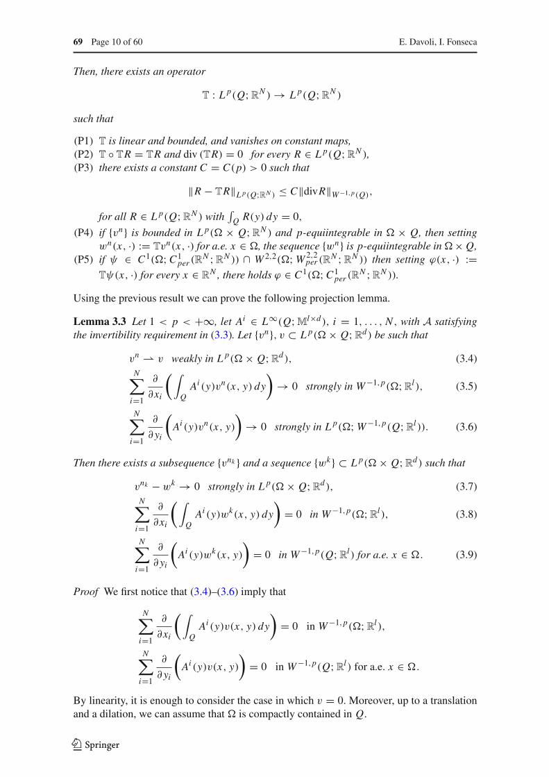
69 Page 10 of 60 E. Davoli, I. Fonseca
Then, there exists an operator
T : L p(Q;RN ) → L p(Q;RN )
such that
(P1) T is linear and bounded, and vanishes on constant maps,(P2) T TR = TR and div (TR) = 0 for every R ∈ L p(Q;RN ),(P3) there exists a constant C = C(p) > 0 such that
‖R − TR‖L p(Q;RN ) ≤ C‖divR‖W−1,p(Q),
for all R ∈ L p(Q;RN ) with∫Q R(y) dy = 0,
(P4) if vn is bounded in L p( × Q;RN ) and p-equiintegrable in × Q, then settingwn(x, ·) := Tvn(x, ·) for a.e. x ∈ , the sequence wn is p-equiintegrable in × Q,
(P5) if ψ ∈ C1(;C1per (R
N ;RN )) ∩ W 2,2(;W 2,2per (R
N ;RN )) then setting ϕ(x, ·) :=Tψ(x, ·) for every x ∈ R
N , there holds ϕ ∈ C1(;C1per (R
N ;RN )).
Using the previous result we can prove the following projection lemma.
Lemma 3.3 Let 1 < p < +∞, let Ai ∈ L∞(Q;Ml×d), i = 1, . . . , N , with A satisfyingthe invertibility requirement in (3.3). Let vn, v ⊂ L p( × Q;Rd) be such that
vn v weakly in L p( × Q;Rd), (3.4)N∑i=1
∂
∂xi
(∫QAi (y)vn(x, y) dy
)→ 0 strongly in W−1,p(;Rl), (3.5)
N∑i=1
∂
∂ yi
(Ai (y)vn(x, y)
)→ 0 strongly in L p(;W−1,p(Q;Rl)). (3.6)
Then there exists a subsequence vnk and a sequence wk ⊂ L p( × Q;Rd) such that
vnk − wk → 0 strongly in L p( × Q;Rd), (3.7)N∑i=1
∂
∂xi
(∫QAi (y)wk(x, y) dy
)= 0 in W−1,p(;Rl), (3.8)
N∑i=1
∂
∂ yi
(Ai (y)wk(x, y)
)= 0 in W−1,p(Q;Rl) for a.e. x ∈ . (3.9)
Proof We first notice that (3.4)–(3.6) imply that
N∑i=1
∂
∂xi
(∫QAi (y)v(x, y) dy
)= 0 in W−1,p(;Rl),
N∑i=1
∂
∂ yi
(Ai (y)v(x, y)
)= 0 in W−1,p(Q;Rl) for a.e. x ∈ .
By linearity, it is enough to consider the case in which v = 0. Moreover, up to a translationand a dilation, we can assume that is compactly contained in Q.
123
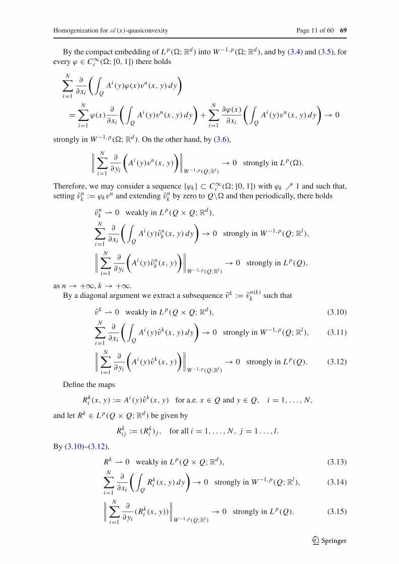
Homogenization for A (x)-quasiconvexity Page 11 of 60 69
By the compact embedding of L p(;Rd) into W−1,p(;Rd), and by (3.4) and (3.5), forevery ϕ ∈ C∞
c (; [0, 1]) there holds
N∑i=1
∂
∂xi
(∫QAi (y)ϕ(x)vn(x, y) dy
)
=N∑i=1
ϕ(x)∂
∂xi
(∫QAi (y)vn(x, y) dy
)+
N∑i=1
∂ϕ(x)
∂xi
(∫QAi (y)vn(x, y) dy
)→ 0
strongly in W−1,p(;Rd). On the other hand, by (3.6),
∥∥∥∥N∑i=1
∂
∂ yi
(Ai (y)vn(x, y)
)∥∥∥∥W−1,p(Q;Rl )
→ 0 strongly in L p().
Therefore, we may consider a sequence ϕk ⊂ C∞c (; [0, 1]) with ϕk 1 and such that,
setting vnk := ϕkvn and extending vnk by zero to Q\ and then periodically, there holds
vnk 0 weakly in L p(Q × Q;Rd),
N∑i=1
∂
∂xi
(∫QAi (y)vnk (x, y) dy
)→ 0 strongly in W−1,p(Q;Rl),
∥∥∥∥N∑i=1
∂
∂ yi
(Ai (y)vnk (x, y)
)∥∥∥∥W−1,p(Q;Rl )
→ 0 strongly in L p(Q),
as n → +∞, k → +∞.By a diagonal argument we extract a subsequence vk := v
n(k)k such that
vk 0 weakly in L p(Q × Q;Rd), (3.10)N∑i=1
∂
∂xi
(∫QAi (y)vk(x, y) dy
)→ 0 strongly in W−1,p(Q;Rl), (3.11)
∥∥∥∥N∑i=1
∂
∂ yi
(Ai (y)vk(x, y)
)∥∥∥∥W−1,p(Q;Rl )
→ 0 strongly in L p(Q). (3.12)
Define the maps
Rki (x, y) := Ai (y)vk(x, y) for a.e. x ∈ Q and y ∈ Q, i = 1, . . . , N ,
and let Rk ∈ L p(Q × Q;Rd) be given by
Rki j := (Rk
i ) j , for all i = 1, . . . , N , j = 1 . . . , l.
By (3.10)–(3.12),
Rk 0 weakly in L p(Q × Q;Rd), (3.13)N∑i=1
∂
∂xi
(∫QRki (x, y) dy
)→ 0 strongly in W−1,p(Q;Rl), (3.14)
∥∥∥∥N∑i=1
∂
∂ yi(Rk
i (x, y))
∥∥∥∥W−1,p(Q;Rl )
→ 0 strongly in L p(Q). (3.15)
123

69 Page 12 of 60 E. Davoli, I. Fonseca
Using Lemma 3.2, we consider the projection operators Tx and Ty onto the kernel of thedivergence operator with respect to x and the divergence operator with respect to y in the setQ. We have ∥∥∥∥Tx
(∫QRk(x, y) dy −
∫Q
∫QRk(w, y) dy dw
)
−(∫
QRk(x, y) dy −
∫Q
∫QRk(w, y) dy dw
)∥∥∥∥L p(Q;Rd )
≤ C
∥∥∥∥N∑i=1
∂
∂xi
(∫QRki (x, y) dy
)∥∥∥∥W−1,p(Q;Rl )
, (3.16)
and ∥∥∥∥Ty
(Rk(x, y) −
∫QRk(x, z) dz
)−(Rk(x, y) −
∫QRk(x, z) dz
)∥∥∥∥L p(Q×Q;Rd )
≤ C
∥∥∥∥∥∥∥∥
N∑i=1
∂
∂ yi(Rk
i (x, y))
∥∥∥∥W−1,p(Q;Rl )
∥∥∥∥L p(Q)
, (3.17)
which in turn yields∥∥∥∥∫QTy
(Rk(x, y) −
∫QRk(x, z) dz
)dy
∥∥∥∥L p(Q;Rd )
=∥∥∥∥∫Q
[Ty
(Rk(x, y) −
∫QRk(x, z) dz
)−(Rk(x, y) −
∫QRk(x, z) dz
)]dy
∥∥∥∥L p(Q;Rd )
≤ C
∥∥∥∥∥∥∥∥
N∑i=1
∂
∂ yi(Rk
i (x, y))
∥∥∥∥W−1,p(Q;Rl )
∥∥∥∥L p(Q)
. (3.18)
Set
Sk(x, y) := Ty
(Rk(x, y) −
∫QRk(x, z) dz
)−∫Q
(Ty
(Rk(x, z) −
∫QRk(x, ξ) dξ
))dz
+ Tx
(∫QRk(x, z) dz −
∫Q
∫QRk(w, z) dz dw
)+∫Q
∫QRk(w, z) dz dw
for a.e. (x, y) ∈ Q × Q. Combining (3.13)–(3.16), we deduce the inequality
‖Rk − Sk‖L p(Q×Q;Rd )
≤∥∥∥∥Ty
(Rk(x, y) −
∫QRk(x, z) dz
)−(Rk(x, y) −
∫QRk(x, z) dz
)∥∥∥∥L p(Q×Q;Rd )
+∥∥∥∥Tx
(∫QRk(x, z) dz −
∫Q
∫QRk(w, z) dz dw
)
−(∫
QRk(x, z) dz −
∫Q
∫QRk(w, z) dz dw
)∥∥∥∥L p(Q;Rd )
+∥∥∥∥∫QTy
(Rk(x, z) −
∫QRk(x, ξ) dξ
)dz
∥∥∥∥L p(Q;Rd ))
+∣∣∣∣∫Q
∫QRk(x, y) dy dx
∣∣∣∣,(3.19)
123

Homogenization for A (x)-quasiconvexity Page 13 of 60 69
whose right-hand-side converges to zero as k → +∞. On the other hand, by Lemma 3.2there holds
N∑i=1
∂Skir (x, y)
∂ yi= 0 in W−1,p(Q) for a.e. x ∈ Q, (3.20)
N∑i=1
∂
∂xi
(∫QSkir (x, y) dy
)= 0 in W−1,p(Q), (3.21)
for every k, for all r = 1, . . . , l.Finally, define
wk(x, y) := A(y)−1
⎛⎜⎝
Sk1 (x, y)...
SkN (x, y)
⎞⎟⎠ for a.e. x ∈ and y ∈ R
N
(where the components Ski are defined analogously to the maps Rki ). Properties (3.8) and (3.9)
follow directly from (3.20) and (3.21). Condition (3.7) is a consequence of the boundednessof A−1 (due to (3.3)) and (3.19).
Remark 3.4 By property (P4) in Lemma 3.2, the boundedness of the operators Ai ,i = 1, . . . , N , and the uniform invertibility condition (3.3), it follows that if vn is p-equiintegrable, then wk is p-equiintegrable as well.
In view of property (P5) in Lemma 3.2 if Ai ∈ C∞per(R
N ;Ml×d), i = 1 . . . , N , and
vn ⊂ C∞c (;C∞
per(RN ;Rd)), then the sequence wk constructed in the proof of Lemma
3.2 inherits the same regularity.
In order to characterize the limit differential constraint, for u ∈ L p(;Rd) and n ∈ N weintroduce the classes
CA (n·)u :=
w ∈ L p(; L p
per(RN ;Rd)) :
∫Q
w(x, y) dy = 0 for a.e. x ∈ ,
×N∑i=1
∂
∂xi
(∫QAi (ny)(u(x) + w(x, y)) dy
)= 0 in W−1,p(;Rl),
×N∑i=1
∂
∂ yi
(Ai (ny)(u(x) + w(x, y))
)= 0 in W−1,p(Q;Rl) for a.e. x ∈
,
(3.22)
and
CA (n·) := u ∈ L p(;Rd) : CA (n·)u = ∅. (3.23)
For simplicity we will also adopt the notation CAu := CA (1·)u and CA := CA (1·). Lemma
3.3 allows us to provide a first characterization of the set CA in the case in which Ai ∈C∞
per(RN ;Ml×d), i = 1 . . . , N .
Proposition 3.5 Let 1 < p < +∞. Let Ai ∈ C∞per(R
N ;Ml×d), i = 1, . . . , N, with Asatisfying the invertibility requirement in (3.3). Let CA be the class introduced in (3.23) andlet A div
ε be the operator defined in (3.1). Then
123

69 Page 14 of 60 E. Davoli, I. Fonseca
CA =u ∈ L p(;Rd) : there exists a sequence uε ⊂ L p(;Rd) such that
uε u weakly in L p(;Rd) and A divε uε → 0 strongly in W−1,p(;Rl)
.
(3.24)
Moreover, for every u ∈ CA and w ∈ CAu there exists a sequence uε ⊂ L p(;Rd) suchthat
uε2−s→ u + w strongly two-scale in L p( × Q;Rd),
and
A divε uε → 0 strongly in W−1,p(;Rl).
Proof Denote by D the set in the right-hand side of (3.24). We divide the proof into twosteps.
Step 1 We first show the inclusion
D ⊂ CA .
Let u ∈ D, and let uε ⊂ L p(;Rd) be such that
uε u weakly in L p(;Rd) (3.25)
and
A divε uε → 0 strongly in W−1,p(;Rl). (3.26)
Consider a test function ψ ∈ C1c (;Rl). We have
⟨A div
ε uε, ψ⟩ → 0, (3.27)
where 〈·, ·〉 denotes the duality product between W−1,p(;Rl) and W 1,p′0 (;Rl). By defi-
nition of the operators A divε ,
⟨A div
ε uε, ψ⟩ = −
∫
N∑i=1
Ai(x
ε
)uε(x) · ∂ψ(x)
∂xidx for every ε > 0.
By Proposition 2.2 there exists a map w ∈ L p(; L pper(R
N ;Rd)) with∫Q w(x, y) dy = 0
such that, up to the extraction of a (not relabeled) subsequence
uε2−s v weakly two-scale (3.28)
where
v(x, y) := u(x) + w(x, y), (3.29)
for a.e. x ∈ , y ∈ RN . Hence, by the definition of two-scale convergence,
⟨A div
ε uε, ψ⟩ → −
∫
∫Q
N∑i=1
Ai (y)v(x, y) · ∂ψ(x)
∂xidy dx,
123

Homogenization for A (x)-quasiconvexity Page 15 of 60 69
and by (3.27) we have that
N∑i=1
∂
∂xi
(∫QAi (y)(u(x) + w(x, y)) dy
)= 0 in W−1,p(;Rl). (3.30)
Let now ϕ ∈ C1per(R
N ;Rl), ψ ∈ C1c (), and consider the sequence of test functions
ϕε(x) := εϕ
(x
ε
)ψ(x) for x ∈ R
N .
The sequence ϕε is uniformly bounded in W 1,p′0 (;Rl), therefore by (3.26)
⟨A div
ε uε, ϕε
⟩ → 0, (3.31)
with
⟨A div
ε uε, ϕε
⟩ = −∫
N∑i=1
Ai(x
ε
)uε(x) ·
(∂ϕ
∂yi
(x
ε
)ψ(x) + εϕ
(x
ε
)∂ψ(x)
∂xi
)dx
for every ε. Passing to the subsequence of uε extracted in (3.28), and applying the definitionof two-scale convergence, we obtain
∫
∫Q
N∑i=1
Ai (y)v(x, y) · ∂ϕ(y)
∂yiψ(x) dy dx = 0
for every ϕ ∈ C1per(R
N ;Rl) and ψ ∈ C1c (). By density, this equality still holds for an
arbitrary ϕ ∈ W 1,p′0 (Q;Rl), and so
N∑i=1
∂
∂ yi
(Ai (y)(u(x) + w(x, y))
)= 0 in W−1,p(Q;Rl) for a.e. x ∈ . (3.32)
Combining (3.30) and (3.32), we deduce that u ∈ CA .Step 2 We claim that CA ⊂ D. Let u ∈ CA , let w ∈ CAu , and set
v(x, y) := u(x) + w(x, y) for a.e x ∈ and y ∈ RN .
Let vδ ⊂ C∞c (;C∞
per(RN ;Rd)) be such that
vδ → v strongly in L p( × Q;Rd). (3.33)
The sequence vδ satisfies both (3.5) and (3.6), hence by Lemma 3.3 and Remark 3.4 wecan construct a sequence vδ ⊂ C∞(;C∞
per(RN ;Rd)) such that
vδ → v strongly in L p( × Q;Rd), (3.34)
N∑i=1
∂
∂xi
(∫QAi (y)vδ(x, y) dy
)= 0 in W−1,p(;Rl), (3.35)
andN∑i=1
∂
∂ yi(Ai (y)vδ(x, y)) = 0 in W−1,p(Q;Rl) for a.e. x ∈ . (3.36)
123

69 Page 16 of 60 E. Davoli, I. Fonseca
Consider now the maps
uεδ(x) := vδ
(x,
x
ε
)
for every x ∈ . By Proposition 2.3 we have
uεδ
2−s→ vδ strongly two-scale in L p( × Q;Rd)
as ε → 0, and hence, by Theorem 2.6
Tεuεδ → vδ strongly in L p(RN × Q;Rd) (3.37)
(where Tε is the unfolding operator defined in (2.1)). We observe that by (3.36),
N∑i=1
∂Ai
∂yi
(x
ε
)vδ
(x,
x
ε
)+ Ai
(x
ε
)∂vδ
∂yi
(x,
x
ε
)= 0 (3.38)
for all x ∈ , for every ε and δ. Moreover, by Propositions 2.2 and 2.3,
N∑i=1
Ai(x
ε
)∂vδ
∂xi
(x,
x
ε
)
N∑i=1
∫QAi (y)
∂vδ
∂xi(x, y) dy
=N∑i=1
∂
∂xi
(∫QAi (y)vδ(x, y) dy
)= 0 (3.39)
as ε → 0, weakly in L p(;Rd), where the last equality follows by (3.35). Finally, since
A divε uε
δ(x) =N∑i=1
∂
∂xi
(Ai(x
ε
)uε
δ(x)
)
= 1
ε
N∑i=1
[∂Ai
∂yi
(x
ε
)vδ
(x,
x
ε
)+ Ai
(x
ε
)∂vδ
∂yi
(x,
x
ε
)]
+N∑i=1
Ai(x
ε
)∂vδ
∂xi
(x,
x
ε
),
by (3.38), (3.39), and the compact embedding of L p into W−1,p , we conclude that
A divε uε
δ → 0 strongly in W−1,p(;Rl), (3.40)
as ε → 0. Collecting (3.34), (3.37), and (3.40), we deduce that
limδ→0
limε→0
(‖Tεu
εδ − (u + w)‖L p(×Q) + ‖A div
ε uεδ‖W−1,p(;Rl )
)= 0.
By Attouch’s diagonalization lemma [3, Lemma 1.15 and Corollary 1.16], there exists asubsequence δ(ε) such that
limε→0
(‖Tεu
εδ(ε) − (u + w)‖L p(×Q) + ‖A div
ε uεδ(ε)‖W−1,p(;Rl )
)= 0.
Setting uε := uεδε
, we finally obtain
A divε uε → 0 strongly in W−1,p(;Rl)
123

Homogenization for A (x)-quasiconvexity Page 17 of 60 69
and
uε 2−s→ u + w strongly two-scale in L p( × Q;Rd),
and hence, by Proposition 2.2,
uε u weakly in L p(;Rd).
This yields that u ∈ D and completes the proof of the proposition. Remark 3.6 The regularity of the operators Ai played a key role in Step 2. In the case inwhich Ai ∈ L∞
per(RN ;Ml×d), i = 1, . . . , N , but we have no further smoothness assumptions
on the operators, the argument in Step 1 still guarantees thatu ∈ L p(;Rd) : there exists a sequence uε ⊂ L p(;Rd) such that
uε u weakly in L p(;Rd)
and A divε uε → 0 strongly in W−1,q(;Rl) for every 1 ≤ q < p
⊂ CA . (3.41)
Indeed, arguing as in Step 1 we obtain that there exists w ∈ L p(; L pper(R
N ;Rd)) with∫Q w(x, y) dy = 0, such that
uε2−s u + w weakly two-scale in L p( × Q;Rd),
and
N∑i=1
∂
∂xi
(∫QAi (y)(u(x) + w(x, y)) dy
)= 0 in W−1,q(;Rl)
N∑i=1
∂
∂ yi(Ai (y)(u(x) + w(x, y))) = 0 in W−1,q(Q;Rl) for a.e. x ∈ , (3.42)
for all 1 ≤ q < p. Since u +w ∈ L p(; L pper(R
N ;Rd)), it follows that (3.42) holds also forq = p. Therefore we deduce the inclusion (3.41).
The proof of the opposite inclusion, on the other hand, is not a straightforward conse-quence of Proposition 3.5. In fact, in the case in which the operators Ai are only bounded, thesecond conclusion in Remark 3.4 does not hold anymore, and we are not able to guarantee thatthe projection operator provided by Lemma 3.3 preserves the regularity of smooth functions.Therefore, the measurability of the maps uε
δ is questionable (see [2, discussion below Defin-ition 1.4]). This difficulty will be overcome in Lemma 5.3 by means of an approximation ofthe operators Ai with C∞ operators.
4 Homogenization for smooth operators
We recall that
F rA (n·)(u) := inf
∫
∫Q
f (u(x) + w(x, y)) dy dx : w ∈ CA (n·)u , ‖w‖L p(×Q;Rd ) ≤ r
(4.1)
123

69 Page 18 of 60 E. Davoli, I. Fonseca
for every u ∈ CA (n·)r and r > 0, where
CA (n·)r := v ∈ L p(;Rd) : ∃w ∈ CA (n·)
v with ‖w‖L p(×Q;Rd ) ≤ r,
F rA (n·)(u) :=
F rA (n·)(u) if u ∈ CA (n·)
r ,
+∞ otherwise in L p(;Rd),(4.2)
for every r > 0, and
FA (u) :=
⎧⎪⎪⎨⎪⎪⎩
infr>0 inf
lim infn→+∞ F r
A (n·)(un) : un u weakly in L p(;Rd)
if u ∈ CA ,
+∞ otherwise in L p(;Rd).
(4.3)
Remark 4.1 We observe that for every u ∈ CA there holds
S :=un : un u weakly in L p(;Rd), un ∈ CA (n·) for every n ∈ N
= ∅
and FA (u) < +∞. Indeed, let u ∈ CA and w ∈ CAu . Then a change of variables and theperiodicity of w yield immediately that
∫Q
w(x, ny) dy = 0 for a.e. x ∈
andn∑
i=1
∂
∂xi
(∫Q(Ai (ny)(u(x) + w(x, ny))) dy
)= 0 in W−1,p(;Rl).
Proving that
n∑i=1
∂
∂yi(Ai (ny)(u(x) + w(x, ny))) = 0 in W−1,p(Q;Rl) for a.e. x ∈
is equivalent to showing that
n∑i=1
∂
∂yi(Ai (y)(u(x) + w(x, y))) = 0 in W−1,p(nQ;Rl) for a.e. x ∈ . (4.4)
To this purpose, arguing as in Step 2 of the proof of Proposition 3.5, construct vδ ⊂C∞(; C∞
per(RN ;Rd)) such that
vδ → u + w strongly in L p( × Q;Rd), (4.5)n∑
i=1
∂
∂xi
(∫Q(Ai (ny)vδ(x, y)) dy
)= 0 in W−1,p(;Rl), (4.6)
n∑i=1
∂
∂yi(Ai (y)vδ(x, y)) = 0 in W−1,p(Q;Rl) for a.e. x ∈ . (4.7)
123

Homogenization for A (x)-quasiconvexity Page 19 of 60 69
By the smoothness and the periodicity of vδ there holds
n∑i=1
∂
∂yi(Ai (y)vδ(x, y)) = 0 in W−1,p(nQ;Rl) for a.e. x ∈
and (4.4) follows in view of (4.5). By the previous argument, w(x, ny) ∈ CA (n·)u , therefore
the set S contains always the sequence un := u for every n.
Theorem 4.2 Let 1 < p < +∞. Let Ai ∈ C∞per(R
N ;Ml×d), i = 1, . . . , N, assume that the
operatorA satisfies the invertibility requirement in (3.3), and letA divε be the operator defined
in (3.1). Let f : Rd → [0,+∞) be a continuous function satisfying the growth condition
0 ≤ f (v) ≤ C(1 + |v|p) for every v ∈ Rd , (4.8)
where C > 0. Then, for every u ∈ L p(;Rd) there holds
inf
lim inf
ε→0
∫
f (uε(x)) dx : uε u weakly in L p(;Rd)
and A divε uε → 0 strongly in W−1,p(;Rl)
= inf
lim sup
ε→0
∫
f (uε(x)) dx : uε u weakly in L p(;Rd)
and A divε uε → 0 strongly in W−1,p(;Rl)
= FA (u).
Before starting the proof of Theorem 4.2, we first state without proving a corollary of [16,Lemma 2.15] and one of [14, Lemma 2.8], and we prove an adaptation of [16, Lemma 2.15]to our framework.
Lemma 4.3 Let 1 < p < +∞. Let uε be a bounded sequence in L p(;RN ) such that
div uε → 0 strongly in W−1,p() (4.9)
and
uε u weakly in L p(;RN ).
Then there exists a p-equiintegrable sequence uε such that
div uε = 0 in W−1,p() for every ε,
uε − uε → 0 strongly in Lq(;RN ) for every 1 ≤ q < p,
uε u weakly in L p(;RN ).
Remark 4.4 A direct adaptation of the proof of [16, Lemma 2.15] yields also that the thesisof Lemma 4.3 still holds if we replace (4.9) with the condition
div uε → 0 strongly in W−1,q()
for every 1 ≤ q < p.
Lemma 4.5 Let 1 < p < +∞, and let D ⊂ Q. Let uε ⊂ L p(D;RN ) be p-equiintegrable,with
uε 0 weakly in L p(D;RN ),
123

69 Page 20 of 60 E. Davoli, I. Fonseca
and
div uε → 0 strongly in W−1,p(D).
Then there exists a p-equiintegrable sequence uε ⊂ L p(Q;RN ) such that
uε − uε → 0 strongly in L p(D;RN ),
uε → 0 strongly in L p(Q\D;RN ),
div uε = 0 in W−1,p(Q),
‖uε‖L p(Q;RN ) ≤ C‖uε‖L p(D;RN ),∫Quε(x) dx = 0 for every ε.
More generally, we have
Lemma 4.6 Let 1 < p < +∞, u ∈ L p(;Rd) and let uε ⊂ L p(;Rd) be such that
uε u weakly in L p(;Rd) (4.10)
A divε uε → 0 strongly in W−1,p(;Rl). (4.11)
Then there exists a p-equiintegrable sequence uε such that
uε u weakly in L p(;Rd),
A divε uε → 0 strongly in W−1,q(;Rl) for every 1 ≤ q < p,
uε − uε → 0 strongly in Lq(;Rd) for every 1 ≤ q < p.
The following propositions is a corollary of [14, Proposition 3.5 (ii)].
Proposition 4.7 Let f : Rd → [0,+∞) be a continuous map satisfying (4.8) for some
1 < p < +∞. Let uε ⊂ L p(;Rd) be a bounded sequence and let uε ⊂ L p(;Rd) bep-equiintegrable and such that
uε − uε → 0 in measure.
Then
lim infε→0
∫
f (uε(x)) dx ≥ lim infε→0
∫
f (uε(x)) dx .
Moreover, if g : RN × Rd → [0,+∞) satisfies
(i) g(·, ξ) is measurable and Q-periodic for every ξ ∈ Rd ,
(ii) g(y, ·) is continuous for a.e. y ∈ RN ,
(iii) there exists a constant C such that
0 ≤ g(y, ξ) ≤ C(1 + |ξ |p) for a.e. y ∈ RNand ξ ∈ R
d ,
then
lim infε→0
∫
g
(x
ε, uε(x)
)dx ≥ lim inf
ε→0
∫
g
(x
ε, uε(x)
)dx .
The next proposition is another corollary of [14, Proposition 3.5 (ii)].
Proposition 4.8 Let 1 ≤ p < +∞ and λ ∈ (0, 1]. Let g : RN × Rd → [0,+∞) be such
that
123

Homogenization for A (x)-quasiconvexity Page 21 of 60 69
(i) g(·, ξ) is measurable and Q-periodic for every ξ ∈ Rd ,
(ii) g(y, ·) is continuous for a.e. y ∈ RN ,
(iii) there exists a constant C such that
0 ≤ g(y, ξ) ≤ C(1 + |ξ |p) for a.e. y ∈ RNand ξ ∈ R
d ,
and let V be a p-equiintegrable subset of L p( × Q;Rd). Then there exists a constant Csuch that
∥∥∥∥g(y
λ, v1(x, y)
)− g
(y
λ, v2(x, y)
)∥∥∥∥L1(×Q)
≤ C‖v1 − v2‖L p(×Q;Rd )
for every v1, v2 ∈ V .
We now start the proof of Theorem 4.2. First we prove the liminf inequality. The argumentrelies on the use of the unfolding operator (see Sect. 2.2 and [14, Appendix A] and thereferences therein).
Proposition 4.9 Under the assumptions of Theorem 4.2 for every u ∈ L p(;Rd) thereholds
inf
lim inf
ε→0
∫
f (uε(x)) dx : uε u weakly in L p(;Rd)
and A divε uε → 0 strongly in W−1,p(;Rl)
≥ FA (u). (4.12)
Proof Let CA be the class introduced in (3.23). We first notice that, by Proposition 3.5, ifu ∈ L p(;Rd)\CA then
uε ⊂ L p(;Rd) : uε u weakly in L p(;Rd)
and A divε uε → 0 strongly in W−1,p(;Rl)
= ∅,
hence (4.12) follows trivially.Define g : RN × R
d → [0,+∞) as
g(y, ξ) = f (A(y)−1ξ) for every y ∈ RN , and ξ ∈ R
d .
By the continuity of f , g is measurable with respect to the first variable (it is the compositionof a continuous function with a measurable one), and continuous with respect to the secondvariable. By (4.8), there holds
0 ≤ g(y, ξ) ≤ C(1 + |A(y)−1ξ |p) ≤ C(1 + |ξ |p), (4.13)
where the last inequality follows by the uniform invertibility assumption (3.3). We divide theproof of the proposition into five steps.
123

69 Page 22 of 60 E. Davoli, I. Fonseca
Step 1 We first show that for every u ∈ CA there holds
inf
lim inf
ε→0
∫
f (uε(x)) dx : uε u weakly in L p(;Rd)
and A divε uε → 0 strongly in W−1,p(;Rl)
≥ infw∈CA
u
inf
lim infn→+∞
∫
g
(x
εn, vεn (x)
)dx :
vεn
∫QA(y)(u(x) + w(x, y)) dy weakly in L p(;Rd),
div vεn → 0 strongly in W−1,p(;Rl),
and A(
x
εn
)−1
vεn u weakly in L p(;Rd)
. (4.14)
Indeed let u ∈ CA and let uε be as in (4.14). Up to the extraction of a subsequence εn,
lim infε→0
∫
f (uε(x)) dx = limn→+∞
∫
f (uεn (x)) dx,
and by Proposition 2.2 there exists w ∈ CAu such that
uεn
2−s u + w weakly two-scale in L p( × Q;Rd). (4.15)
By the definition of g it is straightforward to see that
limn→+∞
∫
f (uεn (x)) dx = limn→+∞
∫
g
(x
εn,A
(x
εn
)uεn (x)
)dx .
Setting vεn := A(
xεn
)uεn , in view of the assumptions on uε in (4.14), it follows that
div vεn =N∑i=1
∂
∂xi
(Ai(
x
εn
)uεn (x)
)→ 0 strongly in W−1,p(;Rl),
and
A(
x
εn
)−1
vεn u weakly in L p(;Rd). (4.16)
Finally, by (4.15) for every ϕ ∈ L p′(;Rd) there holds
limn→+∞
∫
vεn (x) · ϕ(x) dx = limn→+∞
∫
uεn (x) · A(
x
εn
)T
ϕ(x) dx
=∫
∫Q(u(x) + w(x, y)) · A(y)Tϕ(x) dy dx .
This completes the proof of (4.14).
123

Homogenization for A (x)-quasiconvexity Page 23 of 60 69
Step 2 We claim that
infw∈CA
u
inf
lim infn→+∞
∫
g
(x
εn, vεn (x)
)dx :
vεn
∫QA(y)(u(x) + w(x, y)) dy weakly in L p(;Rd),
div vεn → 0 strongly in W−1,p(;Rl),
and A(
x
εn
)−1
vεn u weakly in L p(;Rd)
≥ infw∈CA
u
inf
lim infn→+∞
∫
g
(x
εn,
∫QA(y)(u(x) + w(x, y)) dy + vεn (x)
)dx :
vεn is p-equiintegrable,
vεn 0 weakly in L p(;Rd),
div vεn = 0 in W−1,p(;Rl), and
A(
x
εn
)−1
vεn u(x) −(∫
QA(z)−1 dz
)∫QA(y)(u(x) + w(x, y)) dy
weakly in L p(;Rd)
. (4.17)
Let vεn be as in (4.17). By Lemma 4.3, we construct a p-equiintegrable sequence vεn suchthat
div vεn = 0 in W−1,p(;Rl), (4.18)
vεn − vεn → 0 strongly in Lq(;Rd) for every 1 ≤ q < p, (4.19)
vεn
∫QA(y)(u(x) + w(x, y)) dy weakly in L p(;Rd). (4.20)
Moreover, by Proposition 4.7,
limn→+∞
∫
g
(x
εn, vεn (x)
)dx ≥ lim inf
n→+∞
∫
g
(x
εn, vεn (x)
)dx .
By (4.20) and by the uniform invertibility assumption (3.3), there exists a constant C suchthat
∥∥∥∥A(
x
εn
)−1
vεn
∥∥∥∥L p(;Rd )
≤ C for every n.
Therefore, there exists a map φ ∈ L p(;Rd) such that, up to the extraction of a (not relabeled)subsequence,
A(
x
εn
)−1
vεn φ weakly in L p(;Rd). (4.21)
By the properties of vεn in (4.17) and (4.19), the convergence in (4.21) holds for the entiresequence vεn and
φ = u.
123

69 Page 24 of 60 E. Davoli, I. Fonseca
Claim (4.17) follows by setting
vεn (x) := vεn −∫QA(y)(u(x) + w(x, y)) dy for a.e. x ∈ .
Indeed, by (4.20) we have
vεn 0 weakly in L p(;Rd),
and since w ∈ CAu , by (4.18)
div vεn = 0 in W−1,p(;Rl).
Finally,
A(
x
εn
)−1
vεn (x) = A(
x
εn
)−1
vεn (x) − A(
x
εn
)−1 ∫QA(y)(u(x) + w(x, y)) dy
for a.e. x ∈ , therefore by (4.21) and Riemann–Lebesgue lemma (see e.g. [15]),
A(
x
εn
)−1
vεn u(x) −(∫
QA(z)−1 dz
)∫QA(y)(u(x) + w(x, y)) dy
weakly in L p(;Rd).
Step 3 We show that for every w ∈ CAu and every p-equiintegrable sequence vεn satisfying
vεn 0 weakly in L p(;Rd), (4.22)
div vεn = 0 in W−1,p(;Rl), (4.23)
A(
x
εn
)−1
vεn u(x) −(∫
QA(z)−1 dz
)∫QA(y)(u(x) + w(x, y)) dy (4.24)
weakly in L p(;Rd), there exists a p-equiintegrable family vν,n : ν ∈ N, n ∈ N such that
div vν,n = 0 in W−1,p(;Rl), (4.25)
vν,n 0 weakly in L p(;Rd) as n → +∞, (4.26)
A(
ν
⌊1
νεn
⌋x
)−1
vν,n(x) u −(∫
QA(z)−1 dz
)∫QA(y)(u(x) + w(x, y)) dy
(4.27)
weakly in L p(;Rd), as n → +∞ and
lim infn→+∞
∫
g
(x
εn,
∫QA(y)(u(x) + w(x, y)) dy + vεn (x)
)dx
≥ supν∈N
lim infn→+∞
∫
g
(ν
⌊1
νεn
⌋x,∫QA(y)(u(x) + w(x, y)) dy + vν,n(x)
)dx . (4.28)
To prove the claim we argue as in [14, Proposition 3.8]. Fix ν ∈ N, let
θν,n := νεn
⌊1
νεn
⌋∈ [0, 1]
and set
kν,n := θν,n
νεn∈ N0.
123
Homogenization for A (x)-quasiconvexity Page 25 of 60 69
We notice that
θν,n → 1 as n → +∞. (4.29)
Without loss of generality, we can assume that ⊂⊂ Q. By Lemma 4.5 we extend everymap vεn to a map ˜vεn ∈ L p(Q;Rd) such that ˜vεn is p-equiintegrable, and satisfies thefollowing properties
˜vεn − vεn → 0 strongly in L p(;Rd),
˜vεn → 0 strongly in L p(Q\;Rd),
div ˜vεn = 0 in W−1,p(Q;Rl). (4.30)
In particular, by (4.24) and (4.30) it follows that
A(
x
εn
)−1 ˜vεn (x) u(x) −(∫
QA(z)−1 dz
)∫QA(y)(u(x) + w(x, y)) dy (4.31)
weakly in L p(;Rd). By Proposition 4.7 and the definition of θν,n and kν,n ,
lim infn→+∞
∫
g
(x
εn,
∫QA(y)(u(x) + w(x, y)) dy + vεn (x)
)dx
≥ lim infn→+∞
∫
g
(νkν,n
θν,nx,∫QA(y)(u(x) + w(x, y)) dy + ˜vεn (x)
)dx . (4.32)
For ′ ⊂⊂ fixed, there holds θν,n′ ⊂ for n large enough. Since g is nonnegative (see
(4.13)), by (4.32) we have
lim infn→+∞
∫
g
(x
εn,
∫QA(y)(u(x) + w(x, y)) dy + vεn (x)
)dx
≥ lim infn→+∞
∫θν,n′
g
(νkν,n
θν,nx,∫QA(y)(u(x) + w(x, y)) dy + ˜vεn (x)
)dx
= lim infn→+∞(θν,n)
N∫
′g
(νkν,nx,
∫QA(y)(u(θν,nx) + w(θν,nx, y)) dy + ˜vεn (θν,nx)
)dx
≥ lim infn→+∞
∫′
g
(νkν,nx,
∫QA(y)(u(x) + w(x, y)) dy + ˜vεn (θν,nx)
)dx (4.33)
where the last inequality follows by (4.29), and since
u(θν,nx) + w(θν,nx, y) − u(x) − w(x, y) → 0 strongly in L p( × Q;Rd).
Letting ′ tend to , by the p-equiintegrability of ˜vεn , there holds
lim infn→+∞
∫
g
(x
εn,
∫QA(y)(u(x) + w(x, y)) dy + vεn (x)
)dx
≥ lim infn→+∞
∫
g
(νkν,nx,
∫QA(y)(u(x) + w(x, y)) dy + ˜vεn (θν,nx)
)dx . (4.34)
Set
vν,n(x) := ˜vεn (θν,nx) for a.e. x ∈ , ν ∈ N and n ≥ n0(ν),
123

69 Page 26 of 60 E. Davoli, I. Fonseca
where n0(ν) is big enough so that θν,n ⊂ Q for n ≥ n0(ν). Inequality (4.28) is a directconsequence of (4.34). The p-equiintegrability of vν,n, (4.25), and (4.26) follow in view of(4.29) and (4.30).
To conclude the proof of the claim it remains to establish (4.27). We first remark that,
by (3.3) and (4.26), the sequence
A(
ν
⌊1
νεn
⌋x
)−1
vν,n(x)
is uniformly bounded in
L p(;Rd). Therefore, there exists a map L ∈ L p(;Rd) such that, up to the extractionof a (not relabeled) subsequence, there holds
A(
ν
⌊1
νεn
⌋x
)−1
vν,n(x) L(x) weakly in L p(;Rd). (4.35)
Let ϕ ∈ C∞c (;Rd). Then,
∫
A(
ν
⌊1
νεn
⌋x
)−1
vν,n(x) · ϕ(x) dx →∫
L(x) · ϕ(x) dx . (4.36)
For n big enough, θν,n supp ϕ ⊂ . Hence,
∫
A(
ν
⌊1
νεn
⌋x
)−1
vν,n(x) · ϕ(x) dx
= 1
(θν,n)N
∫θν,n supp ϕ
A(
y
εn
)−1 ˜vεn (y) · ϕ
(y
θν,n
)dy
= 1
(θν,n)N
∫
A(
y
εn
)−1 ˜vεn (y) ·(
ϕ
(y
θν,n
)− ϕ(y)
)dy
+ 1
(θν,n)N
∫
A(
y
εn
)−1 ˜vεn (y) · ϕ(y) dy. (4.37)
By (3.3) the first term in the right-hand side of (4.37) is bounded by
∣∣∣∣ 1
(θν,n)N
∫
A(
y
εn
)−1 ˜vεn (y) ·(
ϕ
(y
θν,n
)− ϕ(y)
)dy
∣∣∣∣≤ C‖ ˜vεn‖L p(;Rd )‖∇ϕ‖L∞(;Md×N ) sup
y∈
∣∣∣∣ y
θν,n− y
∣∣∣∣,
which is infinitesimal as n → +∞ due to (4.29). By (4.29) and (4.31), the second term inthe right-hand side of (4.37) satisfies
limn→+∞
1
(θν,n)N
∫
A(
y
εn
)−1 ˜vεn (y) · ϕ(y) dy
=∫
[u(x) −
∫QA(z)−1 dz
∫QA(y)(u(x) + w(x, y)) dy
]· ϕ(x) dx .
Arguing by density, we conclude that
L(x) = u(x) −(∫
QA(z)−1 dz
)∫QA(y)(u(x) + w(x, y)) dy for a.e. x ∈
and (4.35) holds for the entire sequence. This completes the proof of (4.27).
123

Homogenization for A (x)-quasiconvexity Page 27 of 60 69
Step 4 We claim that for every w ∈ CAu , and every p-equiintegrable family vν,n : ν ∈ N, n ∈N satisfying (4.25)–(4.27), there exists a p-equiintegrable family wν,n : ν ∈ N, n ∈ Nsuch that
divy wν,n(x, y) :=N∑i=1
∂wν,n
∂yi(x, y) = 0 in W−1,p(Q;Rl) for a.e. x ∈ , (4.38)
wν,n 0 weakly in L p( × Q;Rd), as n → +∞, (4.39)∫Q
wν,n(x, y) dy = 0 for a.e. x ∈ , (4.40)
A(⌊
1
νεn
⌋y
)−1
wν,n(x, y) u(x) −(∫
QA(z)−1 dz
)∫QA(y)(u(x) + w(x, y)) dy
(4.41)
weakly in L p(;Rd) as n → +∞ and ν → +∞, in this order,and
lim infn→+∞
∫
g
(ν
⌊1
νεn
⌋x,∫QA(y)(u(x) + w(x, y)) dy + vν,n(x)
)dx
≥ lim infn→+∞
∫
∫Qg
(⌊1
νεn
⌋y,∫QA(z)(u(x) + w(x, z)) dz + wν,n(x, y)
)dy dx + σν,
(4.42)
where σν → 0 as ν → +∞. Let vν,n be as above. We argue similarly to [14, Proof ofProposition 3.9]. We extend u, w, and vν,n to 0 outside , and define
Qν,z := 1
νz + 1
νQ, z ∈ Z
N ,
Zν := z ∈ ZN : Qν,z ∩ = ∅,
Iν,n :=∫
g
(ν
⌊1
νεn
⌋x,∫QA(y)(u(x) + w(x, y)) dy + vν,n(x)
)dx .
By a change of variables, since g(·, 0) = 0 by (4.13), and by the periodicity of g in its firstvariable, we obtain the following chain of equalities
Iν,n =∑z∈Zν
1
νN
∫Qg
(ν
⌊1
νεn
⌋(z
ν+ η
ν
),
∫QA(y)
(u
(z
ν+ η
ν
)+ w
(z
ν+ η
ν, y
))dy
+ vν,n
(z
ν+ η
ν
))dη
=∑z∈Zν
∫Qν,z
∫Qg
(⌊1
νεn
⌋η,
∫QA(y)
(u
(⌊νx
⌋
ν+ η
ν
)+ w
(⌊νx
⌋
ν+ η
ν, y
))dy
+ vν,n
(⌊νx
⌋
ν+ η
ν
))dη dx
=∑z∈Zν
∫Qν,z
∫Qg
(⌊1
νεn
⌋η,
∫QA(y)(u(x) + w(x, y)) dy + T 1
νvν,n(x, η)
)dη dx + σν
123

69 Page 28 of 60 E. Davoli, I. Fonseca
where T 1ν
is the unfolding operator defined in (2.1), and
σν :=∑z∈Zν
∫Qν,z
∫Q
g
(⌊1
νεn
⌋η,
∫QA(y)
(u
(⌊νx
⌋
ν+ η
ν
)+ w
(⌊νx
⌋
ν+ η
ν, y
))dy
+ T 1νvν,n(x, η)
)−g
(⌊1
νεn
⌋η,
∫QA(y)(u(x)+w(x, y)) dy+T 1
νvν,n(x, η)
)dη dx .
By Proposition 2.7,∥∥∥∥∫QA(y)(u(x)+w(x, y)) dy−
∫QA(y)
(T 1
νu(x, η)+T 1
νw((x, η), y)
)dy
∥∥∥∥L p(×Q;Rd )
→ 0
as ν → +∞. Moreover, by Proposition 2.7, the sequence∫
QA(y)(u(x) + w(x, y)) dy −
∫QA(y)
(T 1
νu(x, η) + T 1
νw((x, η), y)
)dy
is p-equiintegrable and∥∥∥∥∫QA(y)(u(x) + w(x, y)) dy
−∫QA(y)
(T 1
νu(x, η) + T 1
νw((x, η), y)
)dy
∥∥∥∥L p
((∪z∈Zν Qν,z\
)×Q;Rd
) → 0
as ν → +∞. Hence, by Proposition 4.8, σν = σν() → 0 as ν → +∞.We set
vν,z,n(y) := T 1νvν,n
(z
ν, y
)for a.e. y ∈ Q, for every z ∈ Zν .
For fixed ν and z ∈ Zν , the sequence vν,z,n is p-equiintegrable. Moreover,
divy vν,z,n = 0 in W−1,p(Q;Rl)
and
vν,z,n 0 weakly in L p(Q;Rd), as n → +∞.
Setting wν,z,n := vν,z,n − ∫Q vν,z,n(y) dy, the sequence wν,z,n ⊂ L p(Q;Rd) is p-
equiintegrable and such that
divy wν,z,n = 0 in W−1,p(Q;Rl),
wν,z,n 0 weakly in L p(Q;Rd), as n → +∞∫Q
wν,z,n(y) dy = 0,
and
wν,z,n − vν,z,n → 0 strongly in L p(Q;Rd), as n → +∞. (4.43)
123
Homogenization for A (x)-quasiconvexity Page 29 of 60 69
By applying again Proposition 4.8 we obtain
∫Qν,z
∫Qg
(⌊1
νεn
⌋y,∫QA(ξ)(u(x) + w(x, ξ)) dξ + T 1
νvν,n
(z
ν, y
))dy dx
≥∫Qν,z
∫Qg
(⌊1
νεn
⌋y,∫QA(ξ)(u(x) + w(x, ξ)) dξ + wν,z,n(y)
)dy dx + τz,ν,n
with
τz,ν,n → 0 as n → +∞.
Therefore, by (4.13) and since
⊂ ∪z∈ZN Qν,z,
we deduce (4.42) with
wν,n(x, y) :=∑z∈Zν
χQν,z∩(x)wν,z,n(y) for a.e. x ∈ , y ∈ Q.
We observe that for ν fixed only a finite number of terms in the sum above are different fromzero, hence properties (4.38), (4.39) and (4.40) follow immediately.
To prove (4.41), we notice that the sequenceA(
⌊1
νεn
⌋y)−1
wν,n(x, y)
is uniformly
bounded in L p( × Q;Rd) by (3.3) and (4.39), therefore it is enough to work witha convergent subsequence and check that the limit is uniquely determined. Fix ϕ ∈C∞c (;C∞
per(Q;Rd)) and set
ψ(x) := u(x) −(∫
QA(z)−1 dz
)∫QA(y)(u(x) + w(x, y)) dy
for a.e. x ∈ , ψ := 0 outside , and
Zνϕ := z ∈ Z
N : (Qν,z × Q) ∩ supp ϕ = ∅.
Then
∫
∫QA(⌊
1
νεn
⌋y
)−1
wν,n(x, y) · ϕ(x, y) dy dx
=∑z∈Zν
ϕ
∫(Qν,z×Q)∩ supp ϕ
A(⌊
1
νεn
⌋y
)−1
wν,z,n(y) · ϕ(x, y) dy dx
=∑z∈Zν
ϕ
∫Q
∫Qν,z
A(⌊
1
νεn
⌋y
)−1
(wν,z,n(y) − vν,z,n(y)) · ϕ(x, y) dy dx
+∑z∈Zν
ϕ
∫Q
∫Qν,z
A(⌊
1
νεn
⌋y
)−1
vν,z,n(y) · ϕ(x, y) dy dx .
123

69 Page 30 of 60 E. Davoli, I. Fonseca
By (3.3), we have
∣∣∣∣∑z∈Zν
ϕ
∫Q
∫Qν,z
A(⌊
1
νεn
⌋y
)−1
(wν,z,n(y) − vν,z,n(y)) · ϕ(x, y) dy dx
∣∣∣∣
≤ C∑z∈Zν
ϕ
‖wν,z,n(y) − vν,z,n(y)‖L p(Q;RN )‖ϕ‖L∞(×Q;Rd ),
which by (4.43) converges to zero as n → +∞ (here we used the fact that the previous seriesis actually a finite sum for every ν ∈ N fixed). On the other hand,
∑z∈Zν
ϕ
∫Q
∫Qν,z
A(⌊
1
νεn
⌋y
)−1
vν,z,n(y) · ϕ(x, y) dy dx
=∑z∈Zν
ϕ
∫Q
∫Qν,z
[A(⌊
1
νεn
⌋y
)−1
T 1νvν,n
(z
ν, y
)− T 1
νψ
(z
ν, y
)]· ϕ(x, y) dy dx
+∑z∈Zν
ϕ
∫Q
∫Qν,z
T 1νψ
(z
ν, y
)· ϕ(x, y) dy dx . (4.44)
By the periodicity of A, the first term in the right-hand side of (4.44) satisfies
limn→+∞
∑z∈Zν
ϕ
∫Q
∫Qν,z
[A(⌊
1
νεn
⌋y
)−1
T 1νvν,n
(z
ν, y
)− T 1
νψ
(z
ν, y
)]· ϕ(x, y) dy dx
= limn→+∞
(1
ν
)N ∑z∈Zν
ϕ
∫Q
∫Q
[A(⌊
1
νεn
⌋y
)−1
vν,n
(z
ν+ y
ν
)− ψ
(z
ν+ y
ν
)]
· ϕ
(z
ν+ η
ν, y
)dy dη
= limn→+∞
∑z∈Zν
ϕ
∫Qν,z
∫Q
[A(⌊
1
νεn
⌋νx
)−1
vν,n(x) − ψ(x)
]
· ϕ
(1
ν
⌊νx
⌋+ 1
νη, νx
)dη dx
= limn→+∞
∫∪z∈Zν
ϕQν,z
[A(⌊
1
νεn
⌋νx
)−1
vν,n(x) − ψ(x)
]
·(∫
Qϕ
(1
ν
⌊νx
⌋+ 1
νη, νx
)dη
)dx .
By (4.27), and recalling that ψ and vν,n have been extended to 0 outside , we concludethat
limn→+∞
∫
∫QA(⌊
1
νεn
⌋y
)−1
wν,n(x, y) · ϕ(x, y) dy dx
=∑z∈Zν
∫Q
∫Qν,z
T 1νψ
(z
ν, y
)· ϕ(x, y) dx dy,
123

Homogenization for A (x)-quasiconvexity Page 31 of 60 69
and so
A(⌊
1
νεn
⌋y
)−1
wν,n(x, y) ∑z∈Zν
χQν,z∩(x)T 1νψ
(z
ν, y
)
weakly in L p( × Q;Rd), as n → +∞. Finally, we claim that
∑z∈Zν
χQν,z∩(x)T 1νψ
(z
ν, y
)→ ψ(x) (4.45)
strongly in L p(;Rd) as ν → +∞.Indeed, let ϕ ∈ L p′
( × Q;Rd). Then by Holder’s inequality∣∣∣∣∫
∫Q
( ∑z∈Zν
χQν,z∩(x)T 1νψ
(z
ν, y
)− ψ(x)
)· ϕ(x, y) dy dx
∣∣∣∣
=∣∣∣∣∑z∈Zν
∫Qν,z∩
∫Q
(T 1
νψ
(z
ν, y
)− ψ(x)
)· ϕ(x, y) dy dx
∣∣∣∣
=∣∣∣∣∑z∈Zν
∫Qν,z∩
∫Q
(ψ
(z
ν+ y
ν
)− ψ(x)
)· ϕ(x, y) dy dx
∣∣∣∣
=∣∣∣∣∑z∈Zν
∫Qν,z∩
∫Q
(ψ
(1
ν
⌊νx
⌋+ y
ν
)− ψ(x)
)· ϕ(x, y) dy dx
∣∣∣∣
=∣∣∣∣∫
∫Q(T 1
νψ(x, y) − ψ(x)) · ϕ(x, y) dy dx
∣∣∣∣≤ ‖T 1
νψ(x, y) − ψ(x)‖L p(×Q;Rd )‖ϕ‖L p′ (×Q;Rd )
.
Property (4.45), and thus (4.41), follow in view of Proposition 2.7.Step 5 By Steps 1–4 it follows that
inf
lim inf
ε→0
∫
f (uε(x)) dx : uε u weakly in L p(;Rd)
and A divε uε → 0 strongly in W−1,p(;Rl)
≥ infw∈Cu
inf
lim infν→+∞ lim inf
n→+∞
∫
∫Qg
(⌊1
νεn
⌋y,∫QA(z)(u(x)
+ w(x, z)) dz + wν,n(x, y)
)dy dx :
divy wν,n(x, y) = 0 in W−1,p(Q;Rl) for a.e. x ∈ ,
wν,n 0 weakly in L p( × Q;Rd) as n → +∞,
A(⌊
1
νεn
⌋y
)−1
wν,n(x, y) u(x) −(∫
QA(z)−1 dz
)∫QA(y)(u(x) + w(x, y)) dy
weakly in L p(;Rd) as n → +∞ and ν → +∞, and∫Q
wν,n(x, y) dy = 0
. (4.46)
123

69 Page 32 of 60 E. Davoli, I. Fonseca
By a diagonalization argument, given wν,n as above we can construct n(ν) such that,setting
εν := εn(ν) wν(x, y) := wν,n(ν),
we obtain the following inequality
inf
lim inf
ε→0
∫
f (uε(x)) dx : uε u weakly in L p(;Rd)
and A divε uε → 0 strongly in W−1,p(;Rl)
≥ infw∈Cu
inf
lim infν→+∞
∫
∫Qg
(⌊1
νεν
⌋y,∫QA(z)(u(x)+w(x, z)) dz+wν(x, y)
)dy dx :
divy wν(x, y) = 0 in W−1,p(Q;Rl) for a.e. x ∈ ,
wν 0 weakly in L p( × Q;Rd) as ν → +∞,
A(⌊
1
νεν
⌋y
)−1
wν(x, y) u(x) −(∫
QA(z)−1 dz
)∫QA(y)(u(x) + w(x, y)) dy
weakly in L p(;Rd) as ν → +∞, and∫Q
wν(x, y) dy = 0
. (4.47)
Associating to every sequence wν as in (4.47) the maps
φν(x, y) :=∫QA(z)(u(x) + w(x, z)) dz + wν(x, y) for a.e. x ∈ and y ∈ Q,
inequality (4.47) can be rewritten as
inf
lim inf
ε→0
∫
f (uε(x)) dx : uε u weakly in L p(;Rd)
and A divε uε → 0 strongly in W−1,p(;Rl)
≥ infw∈Cu
inf
lim infν→+∞
∫
∫Q
f
(A(⌊
1
νεν
⌋y
)−1
φν(x, y)
)dy dx :
divy φν(x, y) = 0 in W−1,p(Q;Rl) for a.e. x ∈ ,
φν
∫QA(z)(u(x) + w(x, z)) dz weakly in L p( × Q;Rd) as ν → +∞,
A(⌊
1
νεν
⌋y
)−1
φν(x, y) u(x) weakly in L p(;Rd) as ν → +∞, and
∫Q
φν(x, z) dz =∫QA(z)(u(x) + w(x, z)) dz
. (4.48)
Finally, for φν as above, considering the maps
vν(x, y) := A(⌊
1
νεn
⌋y
)−1
φν(x, y) for a.e. x ∈ and y ∈ Q,
we deduce that
inf
lim inf
ε→0
∫
f (uε(x)) dx : uε u weakly in L p(;Rd)
123

Homogenization for A (x)-quasiconvexity Page 33 of 60 69
and A divε uε → 0 strongly in W−1,p(;Rl)
≥ infw∈CA
u
inf
lim infν→+∞
∫
∫Q
f (vν(x, y)) dy dx :
divy
(A(⌊
1
νεν
⌋y
)vν(x, y)
)= 0 in W−1,p(Q;Rl) for a.e. x ∈ ,
A(⌊
1
νεν
⌋y
)vν(x, y)
∫QA(z)(u(x)
+ w(x, z)) dz weakly in L p( × Q;Rd) as ν → +∞,
vν(x, y) u(x) weakly in L p( × Q;Rd) as ν → +∞, and∫QA(⌊
1
νεν
⌋z
)vν(x, z) dz =
∫QA(z)(u(x) + w(x, z)) dz
≥ inf
lim infν→+∞
∫
∫Q
f (u(x) + wν(x, y)) dy dx :
divy
(A(⌊
1
νεν
⌋y
)(u(x) + wν(x, y))
)= 0 in W−1,p(Q;Rl) for a.e. x ∈ ,
divx
∫Q
(A(⌊
1
νεν
⌋y
)(u(x) + wν(x, y)
)dy = 0 in W−1,p(;Rl), and
wν(x, y) 0 weakly in L p( × Q;Rd)
. (4.49)
By (4.49) it follows, in particular, that
inf
lim inf
ε→0
∫
f (uε(x)) dx : uε u weakly in L p(;Rd)
and A divε uε → 0 strongly in W−1,p(;Rl)
≥ inf
lim infν→+∞
∫
∫Q
f (uν(x) + wν(x, y)) dy dx :
uν u weakly in L p(;Rd), wν ∈ CA
(⌊1
νεν
⌋·)
uν ,
wν(x, y) 0 weakly in L p( × Q;Rd)
. (4.50)
Fix uν and wν as in (4.50). Then there exists a constant r such that
supν∈N
‖wν‖L p(×Q;Rd ) ≤ r. (4.51)
Therefore, setting
nν :=⌊
1
νεν
⌋,
and
un :=uν if n = nν,
u otherwise,
123

69 Page 34 of 60 E. Davoli, I. Fonseca
we have
lim infν→+∞
∫
∫Q
f (uν(x) + wν(x, y)) dy dx ≥ lim infν→+∞ F r
A
(⌊1
νεν
⌋·)(uν)
= lim infν→+∞ F r
A
(⌊1
νεν
⌋·)(uν) = lim inf
ν→+∞ F rA (nν ·)(unν ) ≥ lim inf
n→+∞ F rA (n·)(un)
≥ inf
lim infn→+∞ F r
A (n·)(un) : un u weakly in L p(;Rd)
. (4.52)
The thesis follows by taking the infimum with respect to r in the right-hand side of (4.52)and by invoking (4.50). Remark 4.10 We point out that the truncation by r in (4.51) and (4.52) will be used in afundamental way. Infact it guarantees that the sequences constructed in the proof of thelimsup inequality (see Proposition 4.12) are uniformly bounded in L p , and hence it allowsus to apply Attouch’s diagonalization lemma (see [3, Lemma 1.15 and Corollary 1.16]) inStep 3 of the proof of Proposition 4.12.
Remark 4.11 In the case in which Ai ∈ L∞(RN ;Ml×d), i = 1, . . . , N , the previous proofyields the inequality
inf
lim inf
ε→0
∫
f (uε(x)) dx : uε u weakly in L p(;Rd)
and A divε uε → 0 strongly in W−1,q(;Rl) for every 1 ≤ q < p
≥ FA (u).
To see that, arguing as in Step 1 we get
inf
lim inf
ε→0
∫
f (uε(x)) dx : uε u weakly in L p(;Rd)
and A divε uε → 0 strongly in W−1,q(;Rl) for every 1 ≤ q < p
≥ infw∈CA
u
inf
lim infn→+∞
∫
g
(x
εn, vεn (x)
)dx :
vεn
∫QA(y)(u(x) + w(x, y)) dy weakly in L p(;Rd),
div vεn → 0 strongly in W−1,q(;Rl) for every 1 ≤ q < p,
and A(
x
εn
)−1
vεn u weakly in L p(;Rd)
.
By Lemma 4.3 and Remark 4.4, inequality (4.17) is replaced by
infw∈CA
u
inf
lim infn→+∞
∫
g
(x
εn, vεn (x)
)dx :
vεn
∫Q
∫QA(y)(u(x) + w(x, y)) dy weakly in L p(;Rd),
123

Homogenization for A (x)-quasiconvexity Page 35 of 60 69
div vεn → 0 strongly in W−1,q(;Rl) for every 1 ≤ q < p,
and A(
x
εn
)−1
vεn u weakly in L p(;Rd)
≥ infw∈CA
u
inf
lim infn→+∞
∫
g
(x
εn,
∫QA(y)(u(x) + w(x, y)) dy + vεn (x)
)dx :
vεn is p-equiintegrable, vεn 0 weakly in L p(;Rd),
div vεn = 0 in W−1,p(;Rl), and
A(
x
εn
)−1
vεn u(x) −(∫
QA(z)−1 dz
)∫QA(y)−1(u(x) + w(x, y)) dy
weakly in L p(;Rd)
.
The result now follows by arguing exactly as in the proof of Proposition 4.9.
We finally prove the limsup inequality in Theorem 4.2.
Proposition 4.12 Under the assumptions of Theorem 4.2, for every u ∈ CA there exists asequence uε ⊂ L p(;Rd) such that
uε u weakly in L p(;Rd), (4.53)
A divε uε → 0 strongly in W−1,p(;Rl), (4.54)
lim supε→0
∫
f (uε(x)) dx ≤ FA (u). (4.55)
Proof We subdivide the proof into three steps.Step 1 Fix n ∈ N. We first show that for every u ∈ CA (n·) ∩ C1(;Rd) and w ∈CA (n·)u ∩ C1(;C1
per(RN ;Rd)) there exists a sequence uε ⊂ L p(;Rd) and a constant C
independent of n and ε such that
uε2−s→ u + w strongly two-scale in L p( × Q;Rd), (4.56)
A divε uε → 0 strongly in W−1,p(;Rl), (4.57)∫
f (uε(x)) dx →∫
∫Q
f (u(x) + w(x, y)) dy dx, (4.58)
as ε → 0, and
supε>0
‖uε‖L p(;Rd ) ≤ C(‖u‖L p(;Rd ) + ‖w‖L p(×Q;Rd )). (4.59)
Define
uε(x) := u(x) + w
(x,
x
nε
)for a.e. x ∈ .
By Proposition 2.3 we have
uε
∫Q(u(x) + w(x, y)) dy = u(x) weakly in L p(;Rd),
uε2−s→ u + w strongly two-scale in L p( × Q;Rd),
f (uε)
∫Q
f (u(x) + w(x, y)) dy weakly in L1(),
123

69 Page 36 of 60 E. Davoli, I. Fonseca
as ε → 0. In particular, we obtain immediately (4.56) and (4.58). Property (4.59) follows by(4.56), Proposition 2.5 and Theorem 2.6. To prove (4.57), we notice that
A divε uε =
N∑i=1
Ai(x
ε
)(∂u(x)
∂xi+ ∂w
∂xi
(x,
x
nε
))
+ 1
nε
(n
∂Ai
∂yi
(x
ε
)(u(x) + w
(x,
x
nε
))+ Ai
(x
ε
)∂w
∂yi
(x,
x
nε
))
=N∑i=1
Ai(nx
nε
)(∂u(x)
∂xi+ ∂w
∂xi
(x,
x
nε
))(4.60)
where in the last equality we used the fact that w ∈ CA (n·)u ∩C1(;C1
per(RN ;Rd)). Applying
Proposition 2.3 we obtain
A divε uε
∫Q
N∑i=1
Ai (ny)
(∂u(x)
∂xi+ ∂w
∂xi(x, y)
)dy weakly in L p(;Rd), (4.61)
and hence strongly in W−1,p(;Rd) by the compact embedding L p → W−1,p. On theother hand, since w ∈ CA (n·)
u , there holds
∫Q
N∑i=1
Ai (ny)
(∂u(x)
∂xi+ ∂w
∂xi(x, y)
)dy =
N∑i=1
∂
∂xi
(∫QAi (ny)(u(x) + w(x, y)) dy
)
= 0. (4.62)
Combining (4.61) with (4.62) we deduce (4).Step 2 We will now extend the construction in Step 1 to the general case where u ∈ CA (n·)and w ∈ CA (n·)
u . Extend u and w by setting them equal to zero outside and × Q,respectively. We claim that we can find sequences uk and wk such that uk ∈ C∞(;Rd),wk ∈ C∞(;C∞
per(RN ;Rd)), and
uk → u strongly in L p(;Rd), (4.63)
wk → w strongly in L p( × Q;Rd), (4.64)
N∑i=1
∂
∂xi
(∫QAi (ny)(uk(x) + wk(x, y)) dy
)→ 0 strongly in W−1,p(;Rl), (4.65)
and
N∑i=1
∂
∂ yi
(Ai (ny)(uk(x) + wk(x, y))
)→ 0 strongly in L p(;W−1,p(Q;Rl)).(4.66)
Indeed, by first regularizing u and w with respect to the variable x , we construct twosequences uk and wk such that uk ∈ C∞(;Rd), wk ∈ C∞(; L p
per(RN ;Rd)), and
uk → u strongly in L p(;Rd),
wk → w strongly in L p( × Q;Rd),
N∑i=1
∂
∂xi
(∫QAi (ny)(uk(x) + wk(x, y)) dy
)→ 0 strongly in W−1,p(;Rl).
123

Homogenization for A (x)-quasiconvexity Page 37 of 60 69
In addition,
N∑i=1
∂
∂ yi
(Ai (ny)(uk(x) + wk(x, y))
)= 0 in W−1,p(Q;Rl) for a.e. x ∈ . (4.67)
Now, by regularizing with respect to y we construct wk, such that wk ∈ C∞(;C∞per(R
N ;Rd)). It is immediate to see that uk and wk satisfy (4.63)–(4.65), and in particular
wk − wk → 0 strongly in L p(; L pper(Q;Rd)). (4.68)
To prove (4.66), consider maps ϕ ∈ L p′() and ψ ∈ W 1,p′
0 (;Rl). By the regularity of theoperators Ai and by (4.67) there holds
∣∣∣∣∫
⟨N∑i=1
∂
∂yi
(Ai (ny)(uk(x) + wk(x, y))
), ψ(y)
⟩ϕ(x) dx
∣∣∣∣
=∣∣∣∣
N∑i=1
∫
∫QAi (ny)(uk(x) + wk(x, y)) · ϕ(x)
∂ψ(y)
∂yidy dx
∣∣∣∣
=∣∣∣∣
N∑i=1
∫
∫QAi (ny)(uk(x) + wk(x, y) − (uk(x) + wk(x, y))) · ϕ(x)
∂ψ(y)
∂yidy dx
∣∣∣∣≤ C‖wk − wk‖L p(×Q;Rd )‖ψ‖
W 1,p′0 (Q;Rd )
‖ϕ‖L p′ ().
Property (4.66) follows now by (4.68).Apply Lemma 3.3 and Remark 3.4 to the sequence uk + wk to construct a sequence
vk ⊂ C1(;C∞per(R
N ;Rd)) such that
vk − (uk + wk) → 0 strongly in L p( × Q;Rd), (4.69)
N∑i=1
∂
∂xi
(∫QAi (ny)vk(x, y) dy
)= 0 in W−1,p(;Rl) (4.70)
and
N∑i=1
∂
∂ yi(Ai (ny)vk(x, y)) = 0 in W−1,p(Q;Rl) for a.e. x ∈ . (4.71)
Consider now the maps
vkε (x) := vk(x,
x
nε
)for a.e. x ∈ .
By Proposition 2.3, arguing as in the proof of (4.59), we observe that
vkε
∫Q
vk(x, y) dy weakly in L p(;Rd),
vkε2−s→ vk strongly two-scale in L p( × Q;Rd),∫
f (vkε (x)) dx →∫
∫Q
f (vk(x, y)) dy dx .
123

69 Page 38 of 60 E. Davoli, I. Fonseca
as ε → 0, and there exists a constant C independent of ε and k such that
‖vkε‖L p(;Rd ) ≤ C‖vk‖L p(×Q;Rd )
for every ε and k. Hence, by (4.63), (4.64), and (4.69), there exists a constant C independentof ε and k such that
‖vkε‖L p(;Rd ) ≤ C(‖u‖L p(;Rd ) + ‖w‖L p(×Q;Rd ))
for every ε and k. In addition, again by Proposition 2.3, proceeding as in the proof of we canestablish the analogues of (4.60)–(4.62) and we conclude that
A divε vkε =
N∑i=1
∂
∂xi
(Ai(x
ε
)vkε (x)
)→
N∑i=1
∂
∂xi
(∫QAi (ny)vk(x, y) dy
)= 0 (4.72)
strongly in W−1,p(;Rl), as ε → 0. Now, by (4.63), (4.64) and (4.69),
vkε2−s→ u + w strongly two-scale in L p( × Q;Rd) (4.73)
as ε → 0 and k → +∞, in this order. Hence, by Theorem 2.6, (4.8), (4.63), (4.64), (4.69),(4.72) and (4.73),
lim supk→+∞
lim supε→0
‖Tεv
kε − (u + w)‖L p(×Q;Rd ) + ‖A div
ε vkε‖W−1,p(;Rl )
+∣∣∣∣∫
f (vkε (x)) dx −∫
∫Q
f (u(x) + w(x, y)) dy dx
∣∣∣∣
= 0.
By Attouch’s diagonalization lemma [3, Lemma 1.15 and Corollary 1.16] we can extract asequence k(ε) such that, setting
vε := vk(ε)ε ,
the sequence vε satisfies (4.56)–(4.59).Step 3 Let u ∈ CA and η > 0. Then FA (u) < +∞ and there exists rη > 0 such that
FA (u) + η > inf
lim infn→+∞ F rη
A (n·)(un) : un u weakly in L p(;Rd)
.
In particular, there exists a sequence uηn ⊂ L p(;Rd) with un ∈ CA (n·) for every n ∈ N,
such that
uηn u weakly in L p(;Rd) (4.74)
as n → +∞, and
FA (u) + η ≥ limn→+∞F rη
A (n·)(uηn) = lim
n→+∞F rηA (n·)(u
ηn).
By the definition of F rηA (n·), for every n ∈ N there exists w
ηn ∈ CA (n·)
uηn
such that
‖wηn‖L p(×Q;Rd ) ≤ rη, (4.75)
and
F rηA (n·)(u
ηn) ≤
∫
∫Q
f (uηn(x) + wη
n (x, y)) dy dx ≤ F rηA (n·)(u
ηn) + 1
n.
123

Homogenization for A (x)-quasiconvexity Page 39 of 60 69
Applying Steps 1 and 2 we construct sequences vηn,ε ⊂ L p( × Q;Rd) such that
supε>0
‖vηn,ε‖L p(×Q;Rd ) ≤ C‖uη
n + wηn‖L p(×Q;Rd ),
vηn,ε uη
n weakly in L p( × Q;Rd),
A divε vη
n,ε → 0 strongly in W−1,p(;Rl),∫
f (vηn,ε(x)) dx →
∫
∫Q
f (uηn(x) + wη
n (x, y)) dy dx, (4.76)
as ε → 0. In addition, by (4.74)–(4.76), the sequence vηn,ε is uniformly bounded in
L p( × Q;Rd). Therefore, by the metrizability of bounded sets in the weak L p topol-ogy and Attouch’s diagonalization lemma [3, Lemma 1.15 and Corollary 1.16] there existsa sequence n(ε) such that, setting
uηε := v
η
n(ε),ε,
properties (4.53) and (4.54) are fulfilled, with
lim supε→0
∫
f (uηε (x)) dx ≤ FA (u) + η.
The thesis follows now by the arbitrariness of η.
5 Homogenization for measurable operators
Here we prove the main result of this paper, concerning the case in which Ai ∈L∞
per(RN ;Ml×d), i = 1, . . . , N .
Theorem 5.1 Let 1 < p < +∞. Let Ai ∈ L∞per(R
N ;Ml×d), i = 1, . . . , N, assume that
the operator A satisfies the invertibility requirement in (3.3), and let A divε be the operator
defined in (3.1). Let f : Rd → [0,+∞) be a continuous function satisfying the growth
condition (4.8). Then, for every u ∈ L p(;Rd) there holds
inf
lim inf
ε→0
∫
f (uε(x)) dx : uε u weakly in L p(;Rd),
and A divε uε → 0 strongly in W−1,q(;Rl) for every 1 ≤ q < p
= inf
lim sup
ε→0
∫
f (uε(x)) dx : uε u weakly in L p(;Rd),
and A divε uε → 0 strongly in W−1,q(;Rl) for every 1 ≤ q < p
= FA (u).
The strategy of the proof consists in constructing a sequence of operators Ak with smoothcoefficients which approximate the operator A , so that Theorem 4.2 can be applied to eachAk . Let ρk be a sequence of mollifiers and consider the operators
Ak : L p(;Rd) → W−1,p(;Rl)
defined as
Akv(x) :=N∑i=1
Aik(x)
∂v(x)
∂xi, (5.1)
123

69 Page 40 of 60 E. Davoli, I. Fonseca
where Aik := Ai ∗ ρk for every i = 1, . . . , N , and for every k. Then Ai
k ∈ C∞per(R
N ;Ml×d),i = 1, . . . , N , for every k,
Aik → Ai strongly in Lm(Q;Ml×d) (5.2)
for 1 ≤ m < +∞, i = 1, . . . , N ,
‖Aik‖L∞(Q;Ml×d ) ≤ ‖Ai‖L∞(Q;Ml×d ) for i = 1, . . . , N , (5.3)
and the operators Ak satisfy the uniform ellipticity condition
Ak(x)λ · λ ≥ α|λ|2 for every λ ∈ Rd , for every k. (5.4)
We first prove two preliminary lemmas. The first one will allow us to approximate everyelement u ∈ CA by sequences uk ⊂ L p(;Rd) with uk ∈ CAk for every k.
Lemma 5.2 Let 1 < p < +∞. LetA be as in Theorem 5.1 and let Ak be the sequence ofoperators with smooth coefficients constructed as above. Let CA be the class introduced in(3.23) and let u ∈ CA . Then there exists a sequence uk ⊂ L p(;Rd) such that uk ∈ CAk
for every k, and
uk → u strongly in L p(;Rd).
Moreover, for every w ∈ CAu there exists a sequence wk ⊂ L p( × Q;Rd) such that
wk ∈ CAkuk
for every k and
wk → w strongly in L p( × Q;Rd).
Proof Let u ∈ CA and let w ∈ CAu . We first construct a sequence vn ⊂ L p( × Q;Rd),defined as
vn(x) := (u(x) + w(x, y))ϕn(x) for a.e. x ∈ , y ∈ Q,
where ϕn ∈ C∞c (; [0, 1]) with ϕn 1. Without loss of generality, up to a dilation and
a translation we can assume that ⊂ Q. Extending each map vn by zero in Q\ and thenperiodically, and arguing as in the proof of Lemma 3.3, it is easy to see that
vn → u + w strongly in L p(Q × Q;Rd),
N∑i=1
∂
∂xi
(∫QAi (y)vn(x, y) dy
)→ 0 strongly in W−1,p(Q;Rl),
N∑i=1
∂
∂ yi
(Ai (y)vn(x, y)
)= 0 in L p(Q;W−1,p(Q;Rl)). (5.5)
By (5.2), (5.3) and the dominated convergence theorem, we also have
Aik(y)v
n(x, y) → Ai (y)vn(x, y) strongly in L p(Q × Q;Rl)
as k → +∞, for every n. Therefore,
N∑i=1
∂
∂xi
(∫QAik(y)v
n(x, y) dy
)→ 0 strongly in W−1,p(Q;Rl),
N∑i=1
∂
∂ yi
(Aik(y)v
n(x, y)
)→ 0 strongly in L p(Q;W−1,p(Q;Rl))
123

Homogenization for A (x)-quasiconvexity Page 41 of 60 69
as k → +∞ and n → +∞, in this order. In particular,
limn→+∞ lim
k→+∞
‖vn − (u + w)‖L p(Q×Q;Rd )
+∥∥∥∥
N∑i=1
∂
∂xi
(∫QAik(y)v
n(x, y) dy
)∥∥∥∥W−1,p(Q;Rl )
+N∑i=1
‖Aik(y)v
n(x, y) − Ai (y)(u(x) + w(x, y))‖L p(Q×Q;Rd )
+∥∥∥∥∥∥∥∥
N∑i=1
∂
∂ yi
(Aik(y)v
n(x, y)
)∥∥∥∥W−1,p(Q;Rl )
∥∥∥∥L p(Q)
= 0,
hence by Attouch’s diagonalization lemma [3, Lemma 1.15 and Corollary 1.16], we canextract a subsequence n(k) such that
vn(k) → u + w strongly in L p( × Q;Rd), (5.6)
Aik(y)v
n(k)(x, y) → Ai (y)(u(x) + w(x, y)) strongly in L p(Q × Q;Rl),
N∑i=1
∂
∂xi
(∫QAik(y)v
n(k)(x, y) dy
)→ 0 strongly in W−1,p(Q;Rl),
N∑i=1
∂
∂ yi
(Aik(y)v
n(k)(x, y)
)→ 0 strongly in L p(Q;W−1,p(Q;Rl)) (5.7)
as k → +∞. Setting
Rik(x, y) := Ai
k(y)vn(k)(x, y) for a.e. (x, y) ∈ Q × Q,
and defining the mappings Rk ∈ L p(Q; L pper(R
N ;Rd)) as
Rki j := (Ri
k) j , for all i = 1, . . . , N , j = 1 . . . , l,
we have that
Rik(x, y) → Ai (y)(u(x) + w(x, y)), i = 1, . . . , N strongly in L p(Q × Q;Rd),
N∑i=1
∂
∂xi
(∫QRik(x, y) dy
)→ 0 strongly in W−1,p(Q;Rl),
N∑i=1
∂
∂ yi(Ri
k(x, y)) → 0 strongly in L p(Q;W−1,p(Q;Rl)).
Therefore, using Lemma 3.2 we argue as in Lemma 3.3 and construct a sequence Sk ∈L p(Q; L p
per(RN ;Rd)), satisfying
123
69 Page 42 of 60 E. Davoli, I. Fonseca
Sk − Rk → 0 strongly in L p(Q × Q;Rd), (5.8)
N∑i=1
∂
∂xi
(∫QSik(x, y) dy
)= 0 in W−1,p(Q;Rl), (5.9)
N∑i=1
∂
∂ yi(Sik(x, y)) = 0 in W−1,p(Q;Rl), for a.e. x ∈ Q. (5.10)
Finally, setting
uk(x) :=∫QAk(y)
−1Sk(x, y) dy for a.e. x ∈
and
wk(x, y) := Ak(y)−1Sk(x, y) − uk(x) for a.e. x ∈ and y ∈ Q,
by (5.9) and (5.10) we deduce that wk ∈ CAkuk
, i.e. uk ∈ CAk for every k. Moreover, by (3.3),(5.6) and (5.8),
‖uk − u‖L p(;Rd ) =∥∥∥∥∫Q(uk(x) + wk(x, y) − (u(x) + w(x, y))) dy
∥∥∥∥L p(;Rd )
≤ C‖uk + wk − (u + w)‖L p(×Q;Rd )
≤ ‖uk + wk − vn(k)‖L p(×Q;Rd ) + ‖vn(k) − (u + w)‖L p(×Q;Rd )
= ‖Ak(y)−1(Sk(x, y) − Rk(x, y))‖L p(×Q;Rd )
+ ‖vn(k) − (u + w)‖L p(×Q;Rd ) → 0.
The convergence of wk to w follows in a similar way. In view of Lemma 5.2 we can prove the analog of Proposition 3.5 in the case in whichAi ∈ L∞
per(RN ;Ml×d), i = 1, . . . , N .
Lemma 5.3 Under the assumptions of Theorem 5.1, there holds
CA =u ∈ L p(;Rd) : there exists a sequence vε ⊂ L p(;Rd) such that
vε u weakly in L p(;Rd)
and A divε vε → 0 strongly in W−1,q(;Rl), for all 1 ≤ q < p
. (5.11)
Proof Let D be the set in the right-hand side of (5.11). The inclusion
D ⊂ CA
follows by Remark 3.6. To prove the opposite inclusion, let u ∈ CA and let w ∈ CAu . ByLemma 5.2 we construct sequences uk ⊂ L p(;Rd) and wk ⊂ L p( × Q;Rd) suchthat uk ∈ CAk for every k, wk ∈ CAk
ukfor every k,
uk → u strongly in L p(;Rd)
and
wk → w strongly in L p( × Q;Rd),
123

Homogenization for A (x)-quasiconvexity Page 43 of 60 69
where Ak is the sequence of operators with smooth coefficients defined in (5.1). By Propo-sition 3.5, for every k there exists a sequence vkε ⊂ L p(;Rd) such that
vkε2−s→ uk + wk strongly 2-scale in L p( × Q;Rd),
A divk,ε vkε :=
N∑i=1
∂
∂xi
(Aik
(x
ε
)vkε (x)
)→ 0 strongly in W−1,p(;Rl)
as ε → 0. Hence, in particular, by Theorem 2.6,
limk→+∞ lim
ε→0‖Tεv
kε − (u + w)‖L p(×Q;Rd ) + ‖A div
k,ε vkε‖W−1,p(;Rl ) = 0.
By Attouch’s diagonalization lemma ([3, Lemma 1.15 and Corollary 1.16]), we can extracta subsequence k(ε) such that
vk(ε)ε
2−s→ u + w strongly 2-scale in L p( × Q;Rd),
Ak(ε),εdivvk(ε)ε → 0 strongly in W−1,p(;Rl)
as ε → 0. A truncation argument analogous to [16, Lemma 2.15] yields a p-equiintegrablesequence vε satisfying
vε u weakly in L p(;Rd),
Ak(ε),εdivvε → 0 strongly in W−1,q(;Rl), (5.12)
for every 1 ≤ q < p.To complete the proof, it remains to prove that
A divε vε → 0 strongly in W−1,q(;Rl) for every 1 ≤ q < p. (5.13)
To this purpose, we first notice that, by (5.2) and by Severini–Egoroff’s theorem, there existsa sequence of measurable sets En ⊂ Q such that |En | ≤ 1
n and
Aik(ε) → Ai uniformly on Q\En (5.14)
for every n = 1, . . . ,+∞. Let η > 0 and 1 ≤ q < p be fixed, and for z ∈ ZN , set
Qε,z := εz + εQ and Zε := z ∈ ZN : Qε,z ∩ = ∅.
By the p-equiintegrability of vε and hence of Tεvε (see Proposition 2.7), and by (5.3),we can assume that
‖Tεvε‖L p((∪z∈Zε Qε,z\)×Q;Rd ) ≤ η, (5.15)
and n is such that
N∑i=1
∫
∫En
|Aik(ε)(y) − Ai (y)|q |Tεvε(x, y)|q dydx
≤ CN∑i=1
(‖Aik(ε)‖qL∞(Q;Ml×d )
+ ‖Ai‖qL∞(Q;Ml×d )
)‖Tεvε(x, y)‖qLq (×En;Rd )≤ η. (5.16)
123

69 Page 44 of 60 E. Davoli, I. Fonseca
We first notice that, by (3.1), there holds∥∥∥∥A divε vε
∥∥∥∥q
W−1,q (;Rl )
≤∥∥∥∥Ak(ε),ε
divvε
∥∥∥∥q
W−1,q (;Rl )
+N∑i=1
∫
∣∣∣∣Aik(ε)
(x
ε
)− Ai
(x
ε
)∣∣∣∣q
|vε(x)|q dx
≤∥∥∥∥Ak(ε),ε
divvε
∥∥∥∥q
W−1,q (;Rl )
+N∑i=1
∫∪z∈Zε (Qε,z∩)
∣∣∣∣Aik(ε)
(x
ε
)− Ai
(x
ε
)∣∣∣∣q
|vε(x)|q dx .
Therefore, by (5.12) we deduce
lim supε→0
∥∥∥∥A divε vε
∥∥∥∥q
W−1,q (;Rl )
≤ lim supε→0
N∑i=1
∫∪z∈Zε (Qε,z∩)
∣∣∣∣Aik(ε)
(x
ε
)− Ai
(x
ε
)∣∣∣∣q
|vε(x)|q dx . (5.17)
Changing variables, using the periodicity of the operators, and extending vε to zero outside, the right-hand side of (5.17) can be estimated as
N∑i=1
∫∪z∈Zε (Qε,z∩)
∣∣∣∣Aik(ε)
(x
ε
)− Ai
(x
ε
)∣∣∣∣q
|vε(x)|q dx
≤ εNN∑i=1
∑z∈Zε
∫Q
|Aik(ε)(y) − Ai (y)|q |vε(εz + εy)|q dy
=N∑i=1
∑z∈Zε
∫Qε,z
∫Q
|Aik(ε)(y) − Ai (y)|q
∣∣∣∣vε
(ε
⌊x
ε
⌋+ εy
)∣∣∣∣q
dydx
=N∑i=1
∫∪z∈Zε Qε,z
∫Q
|Aik(ε)(y) − Ai (y)|q |Tεvε(x, y)|q dydx . (5.18)
By Proposition 2.5, (5.15), and by (5.16), the right-hand side of (5.18) is bounded from aboveas follows
N∑i=1
∫∪z∈Zε Qε,z
∫Q
|Aik(ε)(y) − Ai (y)|q |Tεvε(x, y)|q dydx
≤N∑i=1
∫∪z∈Zε Qε,z\
∫Q
|Aik(ε)(y) − Ai (y)|q |Tεvε(x, y)|q dydx
+N∑i=1
∫
∫En
|Aik(ε)(y) − Ai (y)|q |Tεvε(x, y)|q dydx
+N∑i=1
∫
∫Q\En
|Aik(ε)(y) − Ai (y)|q |Tεvε(x, y)|q dydx
≤ η + CN∑i=1
(‖Aik(ε)‖qL∞(Q;Ml×d )
+ ‖Ai‖qL∞(Q;Ml×d )
)‖Tεvε‖qLq ((∪z∈Zε Qε,z\)×Q;Rd )
123

Homogenization for A (x)-quasiconvexity Page 45 of 60 69
+N∑i=1
‖Aik(ε) − Ai‖q
L∞(Q\En;Ml×d )‖vε‖qLq (;Rd )
≤ Cη + CN∑i=1
‖Aik(ε) − Ai‖L∞(Q\En;Ml×d ). (5.19)
Finally, by (5.14) and collecting (5.17)–(5.19), we obtain
lim supε→0
∥∥∥∥A divε vε
∥∥∥∥q
W−1,q (;Rl )
≤ Cη + limε→0
CN∑i=1
‖Aik(ε) − Ai‖L∞(Q\En;Ml×d ) = Cη
for every η > 0. By the arbitrariness of η we conclude (5.13). Proof of Theorem 4.2 We first notice that by Remark 3.6 the thesis is trivial if u /∈ CA . ByProposition 4.9 and Remark 4.11, for every u ∈ CA there holds
inf
lim inf
ε→0
∫
f (uε(x)) dx : uε u weakly in L p(;Rd),
and A divε uε → 0 strongly in W−1,q(;Rl) for every 1 ≤ q < p
≥ FA (u).
To complete the proof of the theorem, since
inf
lim sup
ε→0
∫
f (uε(x)) dx : uε u weakly in L p(;Rd),
and A divε uε → 0 strongly in W−1,q(;Rl) for every 1 ≤ q < p
≤ inf
lim sup
ε→0
∫
f (uε(x)) dx : uε u weakly in L p(;Rd), uε p-equiintegrable,
and A divε uε → 0 strongly in W−1,q(;Rl) for every 1 ≤ q < p
,
it suffices to show that
inf
lim sup
ε→0
∫
f (uε(x)) dx : uε u weakly in L p(;Rd), uε p-equiintegrable,
and A divε uε → 0 strongly in W−1,q(;Rl) for every 1 ≤ q < p
≤ FA (u).
(5.20)
To prove (5.20), we argue by approximation. Let Ak be the sequence of operatorsconstructed in (5.1) and satisfying (5.2)–(5.4). We first prove that for n, un ∈ CA (n·) andwn ∈ CA (n·)
un fixed,
inf
lim infk→+∞ F2‖wn‖L p (×Q;Rd )
Ak (n·) (un + φk) : φk → 0 strongly in L p(;Rd),
un + φk ∈ CAk (n·) for every k
≤∫
∫Q
f (un(x) + wn(x, y)) dy dx . (5.21)
123

69 Page 46 of 60 E. Davoli, I. Fonseca
Indeed, by Lemma 5.2 there exist sequences uk ⊂ L p(;Rd) and wk ⊂ L p(×Q;Rd),such that uk ∈ CAk (n·), wk ∈ CAk (n·)
ukfor every k,
uk → un strongly in L p(;Rd),
and
wk → wn strongly in L p( × Q;Rd). (5.22)
For k big enough,
F2‖wn‖L p (×Q;Rd )
Ak (n·) (un + (uk − un)) ≤∫
∫Q
f (uk(x) + wk(x, y)) dy dx for every k,
and
lim supk→+∞
F2‖wn‖L p (×Q;Rd )
Ak (n·) (un + (uk(x) − un(x))) ≤∫
∫Q
f (un(x) + wn(x, y)) dy dx,
which in turn implies (5.21).Let now u ∈ CA and η > 0 be fixed. Then, there exist rη > 0 such that
FA (u) + η ≥ inf
lim infn→+∞ Frη
A (n·)(un) : un u weakly in L p(;Rd)
,
and sequences uηn ∈ L p(;Rd), wη
n ∈ L p( × Q;Rd) satisfying
uηn u weakly in L p(;Rd),
wηn ∈ CA (n·)
uηn
for every n,
‖wηn‖L p(×Q;Rd ) ≤ rη for every n, (5.23)
and
FA (u) + 2η ≥ limn→+∞
∫
∫Q
f (uηn(x) + wη
n (x, y)) dy dx .
In particular, by (5.21),
FA (u) + 2η
≥ lim supn→+∞
inf
lim infk→+∞ F2‖wη
n‖L p (×Q;Rd )
Ak (n·) (uηn + φk) : φk → 0 strongly in L p(;Rd),
uηn + φk ∈ CAk (n·) for every k
.
For every n, k, let wηn,k ∈ CAk (n·)
uηn+φk
be such that
‖wηn,k‖L p(×Q;Rd ) ≤ 2‖wη
n‖L p(×Q;Rd ) (5.24)
and
F2‖wηn‖L p (×Q;Rd )
Ak (n·) (uηn + φk) ≤
∫
∫Q
f (uηn(x) + φk(x) + w
ηn,k(x, y)) dy dx
≤ F2‖wηn‖L p (×Q;Rd )
Ak (n·) (uηn + φk) + 1
k.
123

Homogenization for A (x)-quasiconvexity Page 47 of 60 69
Arguing as in Steps 1 and 2 of Proposition 4.12, for every n, k we construct a sequencevη
ε,n,k(x) ⊂ L p(;Rd) such that
‖vηε,n,k‖L p(;Rd ) ≤ C‖uη
n + φk + wηn,k‖L p(×Q;Rd ),
vηε,n,k uη
n + φk weakly in L p(;Rd),
A divk,ε v
ηε,n,k → 0 strongly in W−1,p(;Rl),∫
f (vηε,n,k(x)) dx →
∫
∫Q
f (uηn(x) + φk(x) + w
ηn,k(x, y)) dy dx, (5.25)
as ε → 0, where the constant C is independent of ε, n and k. In particular, (5.23) and(5.24) yield that the sequence vη
ε,n,k is uniformly bounded in L p(;Rd). By (5.25) themetrizability of bounded sets in the weak L p topology and Attouch’s diagonalization lemma([3, Lemma 1.15 and Corollary 1.16]), we can extract subsequences n(ε) and k(ε) suchthat, setting
uε := vη
ε,n(ε),k(ε),
there holds
uε u weakly in L p(;Rd),
A divk(ε)uε → 0 strongly in W−1,p(;Rl),
lim supε→0
∫
f (uε(x)) dx ≤ FA (u) + 2η.
In view of Lemma 4.6 and Proposition 4.7, we can construct a further sequence uε ⊂L p(;Rd), p-equiintegrable and satisfying
uε u weakly in L p(;Rd),
A divk(ε)uε → 0 strongly in W−1,q(;Rl) for every 1 ≤ q < p,
lim supε→0
∫
f (uε(x)) dx ≤ lim supε→0
∫
f (uε(x)) dx ≤ FA (u) + 2η.
Property (5.20) follows now by noticing that exactly the same argument as in the proof of(5.13) yields
A divε uε → 0 strongly in W−1,q(;Rl) for every 1 ≤ q < p,
and by the arbitrariness of η. 5.1 The case of constant coefficients
In this subsection we show that the homogenized energy obtained in Theorem 4.2 reducesto the one identified by Braides, Fonseca and Leoni in [7], in the case in which the operatorsAi , i = 1, . . . , N , are constant, and the constant rank condition (1.3) is satisfied by thedifferential operator A : L p(;Rd) → W−1,p(;Rl) defined as
A u :=N∑i=1
Ai ∂u
∂xifor every u ∈ L p(;Rd).
123

69 Page 48 of 60 E. Davoli, I. Fonseca
In this case the classes CAu and CA defined in (3.22) and (3.23) become, respectively
Cconstu :=
w ∈ L p(; L p
per(RN ;Rd)) :
∫Q
w(x, y) dy = 0 andN∑i=1
Ai ∂w
∂yi(x, y) = 0
and
Cconst :=u ∈ L p(;Rd) : A u = 0
.
Recall that
FA (u) = infr>0
inf
lim infn→+∞ F r
A (un) : un u weakly in L p(;Rd)
.
By definition of A -quasiconvex envelope, for every u ∈ Cconst and r > 0 we have
F rA (u) ≥
∫
QA f (u(x)) dx .
By [16, Theorem3.7], the A -quasiconvex envelope is lower semicontinuous with respect tothe weak L p convergence of A -vanishing maps, hence
inf
lim infn→+∞ F r
A (un) : un u weakly in L p(;Rd)
≥∫
QA f (u(x)) dx
for every r > 0, which yields
FA (u) ≥∫
QA f (u(x)) dx . (5.26)
Conversely, since A is a differential operator with constant coefficients, for every u ∈Cconst the null map belongs to Cconst
u . Hence,∫
f (u(x)) dx ≥ F rA (u) = F r
A (u).
By taking the lower semicontinuous envelope of both sides with respect to the weak L p
convergence of A -vanishing maps we obtain (see [7, Theorem1.1])∫
QA ( f (u(x))) dx ≥ inf
lim infn→+∞ F r
A (un) : un u weakly in L p(;Rd)
≥ FA (u). (5.27)
Combining (5.26) and (5.27) we deduce that
FA (u) =∫
QA f (u(x)) dx .
5.2 The case of a convex energy density
In this subsection we show that if f is convex then the definition of FA (see (4.3)) simplifiesand reduces to a single cell formula.
123
Homogenization for A (x)-quasiconvexity Page 49 of 60 69
For u ∈ L p(;Rd) we introduce the set
CAz,u :=η ∈ L p(; L p
per(RN × R
N ;Rd)) :∫Q
∫Q
η(x, y, z) dz dy = 0 for a.e. x ∈ ,
N∑i=1
∂
∂xi
(∫Q
∫QAi (z)(u(x) + η(x, y, z)) dz dy
)= 0 in W−1,p(;Rl),
N∑i=1
∂
∂zi
(Ai (z)(u(x) + η(x, y, z))
)= 0 in W−1,p(Q;Rl) for a.e. x ∈ and y ∈ Q
.
(5.28)
Remark 5.4 In view of the second differential constraint in (5.28), if η ∈ CAz,u there holds
N∑i=1
∫
∫Q
∫QAi (z)(u(x) + η(x, y, z))ϕ1(x)ϕ2(y) · ∂ϕ3(z)
∂zidz dy dx = 0
for every ϕ1 ∈ C∞c (), ϕ2 ∈ C∞
c (Q), and ϕ3 ∈ W 1,p′0 (Q;Rl). A density argument yields
N∑i=1
∫
∫Q
∫QAi (z)(u(x) + η(x, y, z))ϕ1(x) · ∂ϕ3(z)
∂zidz dy dx = 0
for every ϕ1 ∈ C∞c () and ϕ3 ∈ W 1,p′
0 (Q;Rl), namely
N∑i=1
∂
∂zi
(∫QAi (z)(u(x) + η(x, y, z)) dy
)= 0 in W−1,p(Q;Rl) for a.e. x ∈ .
We recall the notion of “r-two-scale convergence” (reduced two-scale convergence) intro-duced by Neukamm in the framework of dimension reduction problems (see [21]).
Definition 5.5 Let 1 < p < +∞. Let φ ∈ L p( × Q × Q) and φn ⊂ L p( × Q). We
say that φn converges weakly r-two-scale to φ in L p( × Q × Q), φnr−2−s φ, if∫
∫Q
φn(x, y)ϕ(x, y, ny) dy dx →∫
∫Q
∫Q
φ(x, y, z)ϕ(x, y, z) dz dy dx
for every ϕ ∈ C∞c ( × Q;C∞
per(Q)).
We point out that “r-two-scale convergence” is just a particular case of classical two-scaleconvergence, and that the standard properties of two-scale convergence are still valid in thisframework (see [21, Proposition 6.2.5]).
The following characterization holds true.
Theorem 5.6 Let 1 < p < +∞. Let Ai ∈ L∞(Q;Ml×d), i = 1, . . . , N, and let f : Rd →[0,+∞) be convex and satisfying the growth condition
0 ≤ f (v) ≤ C(1 + |v|p) for every v ∈ Rd and some C > 0.
Then for every u ∈ CA there holds
FA (u) = infη∈CA
z,u
∫
∫Q
∫Q
f (u(x) + η(x, y, z)) dz dy dx .
123

69 Page 50 of 60 E. Davoli, I. Fonseca
Proof Let u ∈ CA . We subdivide the proof into two steps.Step 1 We claim that
FA (u) ≥ infη∈CA
z,u
∫
∫Q
∫Q
f (u(x) + η(x, y, z)) dz dy dx . (5.29)
Indeed, in view of (4.1)–(4.3) fix r > 0 and un ∈ L p(;Rd) with un u weakly inL p(;Rd), and un ∈ CA (n·)
r for every n ∈ N. Let wn ⊂ L p( × Q;Rd) be such thatwn ∈ CA (n·)
un for every n ∈ N, supn∈N ‖wn‖L p(×Q;Rd ) ≤ r , and
∫
∫Q
f (un(x) + wn(x, y)) dy dx ≤ F rA (n·)(un) + 1
nfor every n ∈ N.
By the uniform bound on the L p norm of wn there exist w0 ∈ L p( × Q;Rd) andψ0 ∈ L p( × Q × Q;Rd) such that, up to the extraction of (not relabeled) subsequences,there holds (see Proposition 2.2)
wn w0 weakly in L p( × Q;Rd),
and
wnr−2−s ψ0 weakly two-scale in L p( × Q × Q;Rd), (5.30)
with∫Q ψ0(x, y, z) dz = w0(x, y) for a.e. x ∈ and y ∈ Q. In particular, since wn ∈ CA (n·)
un
for every n ∈ N, we have∫Q wn(x, y) dy = 0 for a.e. x ∈ , and for every n ∈ N, which in
turn yields
∫Q
w0(x, y) dy =∫Q
∫Q
ψ0(x, y, z) dz dy = 0 for a.e. x ∈ .
Analogously, by the weak L p convergence of un there exists φ0 ∈ L2( × Q × Q) suchthat, up to the extraction of a (not relabeled) subsequence, there holds
unr−2−s u + φ0 (5.31)
with∫Q
∫Q φ0(x, y, z) = 0 for a.e. x ∈ .
Setting η0 := ψ0 + φ0, an adaptation of the argument in Step 1 of Proposition 3.5 andRemark 3.6, together with the periodicity of the operators Ai , i = 1, . . . , N , allows to passto the limit as n → +∞ in the differential constraints defining the classes CA (n·)
un , and to
deduce that η0 ∈ CAz,u . Indeed, let ϕ ∈ W 1,p′0 (;Rl). Since wn ∈ CA (n·)
un , we have
⟨N∑i=1
∂
∂xi
(∫QAi (ny)(un(x) + wn(x, y)) dy
), ϕ
⟩
= −N∑i=1
∫
∫QAi (ny)(un(x) + wn(x, y)) · ∂ϕ(x)
∂xidy dx = 0
123

Homogenization for A (x)-quasiconvexity Page 51 of 60 69
for every n ∈ N. In view of (5.30) and (5.31) we obtain
limn→+∞
N∑i=1
∫
∫QAi (ny)(un(x) + wn(x, y)) · ∂ϕ(x)
∂xidy dx
=N∑i=1
∫
∫Q
∫QAi (z)(u(x) + η0(x, y, z)) · ∂ϕ(x)
∂xidz dy dx .
Thus, by the arbitrariness of ϕ,
N∑i=1
∂
∂xi
(∫Q
∫QAi (z)(u(x) + η0(x, y, z)) dy dz
)= 0 in W−1,p(;Rl).
The second differential constraint in (5.28) follows by a similar argument.By the convexity of f we use its two-scale L p lower-semicontinuity (see [26, Proposi-
tion1.3]) to deduce that
lim infn→+∞ F r
A (n·)(un) ≥ limn→+∞
∫
∫Q
f (un(x) + wn(x, y)) dy dx
≥∫
∫Q
∫Q
f (u(x) + η0(x, y, z)) dz dy dx
≥ infη∈CA
z,u
∫
∫Q
∫Q
f (u(x) + η(x, y, z)) dz dy dx . (5.32)
Since the same procedure applies to every sequence un as above and to every r > 0, weobtain (5.29).Step 2 We show that for every λ > 0 the following inequality holds true
FA (u) ≤ infη∈CA
z,u
∫
∫Q
∫Q
f (u(x) + η(x, y, z)) dz dy dx + λ. (5.33)
Indeed, let ηλ ∈ CAz,u be such that
∫
∫Q
∫Q
f (u(x) + ηλ(x, y, z)) dz dy dx
≤ infη∈CA
z,u
∫
∫Q
∫Q
f (u(x) + η(x, y, z)) dz dy dx + λ, (5.34)
and set
wn(x, y) :=∫Q
ηλ(x, z, ny) dz for every x ∈ and y ∈ Q.
The fact that ηλ ∈ CAz,u yields
∫Q
wn(x, y) dy = 0 for a.e. x ∈ , (5.35)
123

69 Page 52 of 60 E. Davoli, I. Fonseca
for every n ∈ N. By the periodicity of ηλ and of the operators Ai , i = 1, . . . , N , there holds∫QAi (ny)(u(x) + wn(x, y)) dy =
∫Q
∫QAi (ny)(u(x) + ηλ(x, z, ny)) dz dy
= 1
nN
∫nQ
∫QAi (y)(u(x)+ηλ(x, z, y)) dz dy=
∫Q
∫QAi (y)(u(x) + ηλ(x, z, y)) dz dy,
for a.e. x ∈ . Since ηλ ∈ CAz,u we obtain
N∑i=1
∂
∂xi
(∫QAi (ny)(u(x) + wn(x, y)) dy
)
=N∑i=1
∂
∂xi
(∫Q
∫QAi (y)(u(x) + ηλ(x, z, y)) dz dy
)= 0 (5.36)
in W−1,p(;Rl).As a consequence of Remark 5.4 we deduce that
N∑i=1
∂
∂yi
(Ai (ny)(u(x) + wn(x, y)
)
=N∑i=1
∂
∂yi
∫Q
(Ai (ny)(u(x) + ηλ(x, z, ny))
)dz = 0 (5.37)
in W−1,p(Q;Rl), for a.e. x ∈ . By Jensen’s inequality we have
lim infn→+∞
∫
∫Q
f (u(x) + wn(x, y)) dy dx
≤ limn→+∞
∫
∫Q
∫Q
f (u(x) + ηλ(x, z, ny)) dz dy dx
=∫
∫Q
∫Q
f (u(x) + ηλ(x, z, y)) dz dy dx,
where in the last equality we used the Riemann Lebesgue Lemma with respect to the vari-able y, and Lebesgue Dominated convergence Theorem, taking into account that, due toperiodicity
‖ηλ(x, z, ny)‖L p(×Q×Q;Rd ) = ‖ηλ(x, z, y)‖L p(×Q×Q;Rd )
for all n ∈ N. Now (5.34) yields
FA (u) ≤ inf
lim infn→+∞ F Kη
A (n·)(un) : un u weakly in L p(;Rd)
≤ lim infn→+∞ F Kη
A (n·)(u)
≤ lim infn→+∞
∫
∫Q
f (u(x) + wn(x, y)) dy dx
≤∫
∫Q
∫Q
f (u(x) + ηλ(x, z, y)) dz dy dx
123

Homogenization for A (x)-quasiconvexity Page 53 of 60 69
≤ infη∈CA
z,u
∫
∫Q
∫Q
f (u(x) + η(x, y, z)) dz dy dx + λ,
which in turn implies (5.33). The thesis follows by combining (5.29) and (5.33), and by thearbitrariness of λ. 5.3 Nonlocality of the operator
We end this section with an example that illustrates that, in general, when the operators Ai arenot constant then the functional FA in (4.3) can be nonlocal, even when the energy densityf is convex.
Example 5.7 Let N = d = p = 2 and l = 1, and choose
= (0, 1) × (0, 1).
Let a ∈ C∞per(R), with period (− 1
2 , 12 ), a > −1, and satisfying
∫ 12
− 12
a(s) ds = 0 and∫ 1
2
− 12
a2(s) ds = 1, (5.38)
and consider the operators A1, A2 : R2 → R2 defined as
A1(x) := (1 + a(x2) 0) and A2(x) := (0 1)
for x ∈ R2. We have that
A(y)ξ =(
1 + a(y2) 00 1
)ξ
for ξ ∈ R2 and y ∈ Q, therefore the operator A satisfies the uniform invertibility assumption
(3.3).Consider the function f : R2 → [0,+∞), defined as f (ξ) := |ξ |2 for every ξ ∈ R
2. By(5.38), for n fixed, un ∈ CA (n·) if and only if there exists wn ∈ L2( × Q;R2) such that∫Q wn(x, y) dy = 0, and the following two conditions are satisfied
∂
∂x1
(∫Qa(ny2)w1,n(x, y) dy
)+ div un(x) = 0 in W−1,2(), (5.39)
(1 + a(ny2))∂w1,n(x, y)
∂y1+ ∂w2,n(x, y)
∂y2= 0 in W−1,2(Q) for a.e. x ∈ . (5.40)
Moreover, for every u ∈ L2(;Rd) and w ∈ L2( × Q;R2) with∫Q w(x, y) dy = 0,
there holds∫
∫Q
f (u(x) + w(x, y)) dy =∫
|u(x)|2 dx +∫
∫Q
|w(x, y)|2 dy dx . (5.41)
In view of (5.41), for every r > 0, n ∈ N, and un ∈ CA (n·),
F rA (n·)(un) ≥
∫
|un(x)|2 dx,hence by classical lower-semicontinuity results (see,e.g.,[15, Theorem 5.14]),
FA (u) ≥∫
|u(x)|2 dx for every u ∈ CA . (5.42)
123

69 Page 54 of 60 E. Davoli, I. Fonseca
If 0 ∈ CAu , i.e., div u = 0 (and hence 0 ∈ CA (n·)u for every n), then
F rA (n·)(u) =
∫
|u(x)|2dx
for every n and r , and choosing un = u for every n in (4.3), we deduce that (5.42) holds withequality.
Strict inequality holds in (5.42) if u ∈ CA but div u = 0. Such fields exist, consider forexample,
u(x) :=(−x1
0
)for x ∈ .
Note that the map
w(x, y) :=(a(y2)x1
0
)for every (x, y) ∈ × Q
satisfies w ∈ CAu by (5.38)Assume by contradiction that there exists u ∈ CA , with div u = 0, such that
FA (u) =∫
|u(x)|2 dx . (5.43)
By the definition of FA there exists a sequence rm of real numbers such that
FA (u) = limm→+∞ inf
lim infn→+∞ F rm
A (n·)(un) : un u weakly in L p(;Rd)
.
For every m ∈ N, let umn ⊂ L2(;Rd) be such that
umn u weakly in L2(;Rd)
as n → +∞, and
inf
lim infn→+∞ F rm
A (n·)(un) : un u weakly in L2(;Rd)
+ 1
m≥ lim inf
n→+∞ F rmA (n·)(umn ).
Then
FA (u) = limm→+∞ lim inf
n→+∞ F rmA (n·)(umn ),
and by a diagonal argument we can extract a subsequence n(m) such that, setting um :=umn(m),
FA (u) = limm→+∞F rm
A (n(m)·)(um). (5.44)
By (5.41), for every m there exists wm ∈ CA (n(m)·)um such that ‖wm‖L2(×Q;Rd ) ≤ rm and
F rmA (n(m)·)(um) + 1
m≥∫
∫Q
f (um(x) + wm(x, y)) dy dx
=∫
|um(x)|2 dx +∫
∫Q
|wm(x, y)|2 dy dx . (5.45)
Hence, in view of (5.43), (5.44) and (5.45),∫
|u(x)|2 dx = limm→+∞
(∫
|um(x)|2 dx +∫
∫Q
|wm(x, y)|2 dy dx)
,
123
Homogenization for A (x)-quasiconvexity Page 55 of 60 69
and so
um → u strongly in L2(;Rd), (5.46)
and
wm → 0 strongly in L2( × Q;Rd). (5.47)
By (5.39) and the boundedness of the function a, properties (5.46) and (5.47) yield
div um → 0 strongly in W−1,2()
which in turn implies that div u = 0, contradicting the assumptions on u.We conclude that if u ∈ CA satisfies div u = 0, then
FA (u) =∫
|u(x)|2 dx, (5.48)
whereas if u ∈ CA satisfies div u = 0, then
FA (u) >
∫
|u(x)|2 dx . (5.49)
We now provide an explicit expression for the functional FA . We claim that for everyu ∈ CA there holds
FA (u) =∫
|u(x)|2 dx +∫
|φu (x)|2 dx, (5.50)
where φu ∈ L2() is the unique function satisfying
∫ 10 φ
u (x1, x2) dx1 = 0 for a.e. x2 ∈(0, 1), and ∂φ
u (x)∂x1
= −div u(x) in W−1,2().
To prove (5.50) we first establish a preliminary lemma.
Lemma 5.8 Let n ∈ N, and let v ∈ CA (n·). Then
infw∈CA (n·)(v)
[ ∫
|v(x)|2 dx +∫
∫Q
|w(x, y)|2 dx dy]
=∫
|v(x)|2 dx +∫
|φv (x)|2 dx, (5.51)
where∫ 1
0 φv (x1, x2) dx1 = 0 for a.e. x2 ∈ (0, 1), and ∂φ
v (x)∂x1
= −div v(x) in W−1,2().
Proof We recall that by (5.39) and (5.40), w ∈ CA (n·)(v) if and only if∫Q
w(x, y) dy = 0, for a.e. x ∈ ,
∂
∂x1
(∫Qa(ny2)w1(x, y) dy
)+ div v(x) = 0 in W−1,2(),
(1 + a(ny2))∂w1(x, y)
∂y1+ ∂w2(x, y)
∂y2= 0 in W−1,2(Q) for a.e. x ∈ . (5.52)
By (5.52), the map φv defined in the statement of Lemma 5.8 satisfies
φv (x) =
∫Qa(ny2)w1(x, y) dy −
∫ 1
0
(∫Qa(ny2)w1(x, y) dy
)dx1 for a.e. x ∈ .
123
69 Page 56 of 60 E. Davoli, I. Fonseca
Rewriting w1 as
w1(x, y) := a(ny2)
∫Qa(ny2)w1(x, y) dy + ηw(x, y),
we have ∫Qa(ny2)ηw(x, y) dy = 0,
and hence∫
∫Q
|w(x, y)|2 dx dy =∫
∫Q
|w1(x, y)|2 dx dy +∫
∫Q
|w2(x, y)|2 dx dy
≥∫
(∫Qa(ny2)w1(x, y) dy
)2
dx +∫
∫Q
|ηw(x, y)|2 dx dy
≥∫
|φv (x)|2 dx +
∫
(∫ 1
0
(∫Qa(ny2)w1(x, y) dy
)dx1
)2
dx
≥∫
|φv (x)|2 dx for every w ∈ CA (n·)(v).
In particular, we obtain the lower bound
infw∈CA (n·)(v)
[ ∫
|v(x)|2 dx +∫
∫Q
|w(x, y)|2 dx dy]
≥∫
|v(x)|2 dx +∫
|φv (x)|2 dx .
Property (5.51) follows by observing that (5.38) yields(a(ny2)φ
v (x), 0
)∈ CA (n·)(v).
Let u ∈ CA . Arguing as in the proof of (5.49) there exist a sequence nm ⊂ N, withnm → +∞ as m → +∞, and sequences um ⊂ L2(;R2) and wm ⊂ L2( × Q;R2),such that
um u weakly in L2(;R2),
wm ∈ CA (nm ·)um , (5.53)
and
FA (u) = limm→+∞
∫
|um(x)|2 dx +∫
∫Q
|wm(x, y)|2 dx dy.
In view of Lemma 5.8,
FA (u) ≥ lim supm→+∞
∫
|um(x)|2 dx +∫
|φm(x)|2 dx, (5.54)
where∫ 1
0φm(x1, x2) dx1 = 0, for a.e. x2 ∈ (0, 1), (5.55)
123

Homogenization for A (x)-quasiconvexity Page 57 of 60 69
and
∂φm(x)
∂x1= −div umn (x) in W−1,2(). (5.56)
Since u ∈ CA , there holds FA (u) < +∞, and the sequence φm is uniformly bounded inL2(). Therefore there exists φ
u ∈ L2() such that, up to the extraction of a (not relabeled)subsequence,
φm φu weakly in L2(), (5.57)
where, by (5.53), (5.55) and (5.56),
∫ 12
− 12
φu (x1, x2) dx1 = 0 for a.e. x2 ∈ (0, 1)
and
∂φu (x)
∂x1= −div u(x) in W−1,2().
In particular, by (5.53) and the lower semicontinuity of the L2-norm,
FA (u) ≥∫
|u(x)|2 dx +∫
|φu (x)|2 dx .
To prove the opposite inequality, choose un := u, wn :=(a(ny2)φ
u (x), 0
)for every n ∈ N.
By Lemma 5.8, for r big enough there holds
FrA (n·)(un) =
∫
|u(x)|2 dx +∫
|φu (x)|2 dx .
The characterization (5.50) follows now by the definition of FA .We conclude this example by showing that the functional FA is nonlocal. Indeed, assume
by contradiction thatFA is local. Then for every u ∈ CA we can associate toFA an additiveset function FA (u, ·) on the class O() of open subsets of . In particular, for every pair1,2 ⊂ , with 1 ⊂⊂ 2 ⊂⊂ , and for every u ∈ CA in , there holds
FA (u,) ≤ FA (u,\1) + FA (u,2). (5.58)
Let ξ1, ξ2 ∈ R, with ξ1 = ξ2, and let ε, δ > 0 be such that ε < 12 and δ < 1
2 − ε. Define
1 :=(
12 − ε, 1
2 + ε
)×(
12 − ε, 1
2 + ε
)and
2 :=(
12 − ε − δ, 1
2 + ε + δ
)×(
12 − ε − δ, 1
2 + ε + δ
).
Consider the function
u0(x) :=
⎧⎪⎪⎪⎨⎪⎪⎪⎩
(−ξ1
0
)if x ∈ 1,
(−ξ2
0
)otherwise in .
123

69 Page 58 of 60 E. Davoli, I. Fonseca
We observe u0 belongs to CA , since the map
w0(x, y) :=
⎧⎪⎪⎪⎨⎪⎪⎪⎩
(a(y2)ξ1
0
)if x ∈ 1, y ∈ Q,
(a(y2)ξ2
0
)otherwise in × Q,
satisfies w0 ∈ CAu0. By (5.48), since div u0 = 0 in \1, there holds
FA (u0;\1) =∫
1
|u0(x)|2 dx = (1 − 4ε2)ξ22 . (5.59)
A direct computation yields
φu0
=
⎧⎪⎪⎨⎪⎪⎩
(1 − 2ε)(ξ1 − ξ2) in 1
2ε(ξ2 − ξ1) in [(
0, 12 − ε
)∪(
12 + ε, 1
)] ×
(12 − ε, 1
2 + ε
)
0 otherwise in ,
and
φ2u0
=
⎧⎪⎪⎨⎪⎪⎩
δ(ξ1−ξ2)ε+δ
in 1
ε(ξ2−ξ1)ε+δ
in [(
12 − ε − δ, 1
2 − ε
)∪(
12 + ε, 1
2 + ε + δ
)] ×
(12 − ε, 1
2 + ε
)
0 otherwise in 2.
Therefore,
FA (u0,) =∫
|u0(x)|2 dx +∫
|φu0
(x)|2 dx (5.60)
= 4ε2ξ21 + (1 − 4ε2)ξ2
2 + 4ε2(1 − 2ε)(ξ1 − ξ2)2, (5.61)
and
FA (u0,2) =∫
2
|u0(x)|2 dx +∫
2
|φu0
(x)|2 dx (5.62)
= 4ε2ξ21 + 4δ(δ + 2ε)ξ2
2 + 4ε2δ(ξ1 − ξ2)2
ε + δ. (5.63)
Now (5.58) becomes
4ε2(1 − 2ε)(ξ1 − ξ2)2 ≤ 4δ(δ + 2ε)ξ2
2 + 4ε2δ(ξ1 − ξ2)2
ε + δ
for every ε < 12 and δ < 1
2 − ε. Letting δ → 0 we get
4ε2(1 − 2ε)(ξ1 − ξ2)2 ≤ 0.
Since ξ1 = ξ2, this contradicts the subadditivity of FA (u0, ·) and yields the nonlocality ofFA .
123

Homogenization for A (x)-quasiconvexity Page 59 of 60 69
Acknowledgments The authors thank the Center for Nonlinear Analysis (NSF Grant No. DMS-0635983),where this research was carried out. The research of E. Davoli, and I. Fonseca was funded by the NationalScience Foundation under Grant No. DMS- 0905778. I. Fonseca was also supported by the National ScienceFoundation under Grant No. DMS-1411646. E. Davoli and I. Fonseca acknowledge support of the NationalScience Foundation under the PIRE Grant No. OISE-0967140. E. Davoli is a member of the INDAM-GNAMPAProject 2015 “Critical phenomena in the mechanics of materials: a variational approach”, and was supportedby the Austrian FWF project “Global variational methods for nonlinear evolution equations”.
References
1. Acerbi, E., Fusco, N.: Semicontinuity problems in the calculus of variations. Arch. Rat. Mech. Anal.86(2), 125–145 (1984)
2. Allaire, G.: Homogenization and two-scale convergence. SIAM J. Math. Anal. 23(6), 1482–1518 (1992)3. Attouch, H.: Variational Convergence for Functions and Operators. Applicable Mathematics Series. Pit-
man (Advanced Publishing Program), Boston (1984)4. Ball, J.M.: Convexity conditions and existence theorems in nonlinear elasticity. Arch. Rat. Mech. Anal.
63(4), 337–403 (1976/77)5. Bendsøe, M.P.: Optimization of Structural Topology, Shape, and Material. Springer, Berlin (1995)6. Bensoussan, A., Lions, J.L., Papanicolaou, G.: Asymptotic Analysis for Periodic Structures. AMS Chelsea
Publishing, Providence (2011). (Corrected reprint of the 1978 original)7. Braides, A., Fonseca, I., Leoni, G.: A-quasiconvexity: relaxation and homogenization. ESAIM Control
Optim. Calc. Var. 5, 539–577 (2000). (electronic)8. Cioranescu, D., Damlamian, A., Griso, G.: Periodic unfolding and homogenization. C. R. Math. Acad.
Sci. Paris 335(1), 99–104 (2002)9. Cioranescu, D., Damlamian, A., Griso, G.: The periodic unfolding method in homogenization. SIAM J.
Math. Anal. 40(4), 1585–1620 (2008)10. Cioranescu, D., Donato, P.: An introduction to homogenization. In: Oxford Lecture Series in Mathematics
and its Applications, vol. 17. The Clarendon Press, Oxford University Press, New York (1999)11. Dacorogna, B.: Weak continuity and weak lower semicontinuity of nonlinear functionals. Lecture Notes
in Mathematics, vol. 922. Springer, Berlin (1982)12. Dacorogna, B., Fonseca, I.: A-B quasiconvexity and implicit partial differential equations. Calc. Var.
Partial Differ. Equ. 14(2), 115–149 (2002)13. Davoli, E., Fonseca, I.: Homogenization for A-quasiconvexity with variable coefficients (2016). http://
cvgmt.sns.it/paper/2904/14. Fonseca, I., Krömer, S.: Multiple integrals under differential constraints: two-scale convergence and
homogenization. Indiana Univ. Math. J. 59(2), 427–457 (2010)15. Fonseca, I., Leoni, G.: Modern methods in the calculus of variations: L p spaces. In: Springer Monographs
in Mathematics. Springer, New York (2007)16. Fonseca, I., Müller, S.: A-quasiconvexity, lower semicontinuity, and Young measures. SIAM J. Math.
Anal. 30(6), 1355–1390 (1999). (electronic)17. Lukkassen, D., Nguetseng, G., Wall, P.: Two-scale convergence. Int. J. Pure Appl. Math. 2(1), 35–86
(2002)18. Marcellini, P.: Approximation of quasiconvex functions, and lower semicontinuity of multiple integrals.
Manuscripta Math. 51(1–3), 1–28 (1985)19. Morrey, C.B. Jr.: Multiple integrals in the calculus of variations. Die Grundlehren der mathematischen
Wissenschaften, Band 130. Springer, New York (1966)20. Murat, F.: Compacité par compensation: condition nécessaire et suffisante de continuité faible sous une
hypothèse de rang constant. Ann. Scuola Norm. Sup. Pisa Cl. Sci. (4) 8(1), 69–102 (1981)21. Neukamm, S.: Homogenization, linearization and dimension reduction in elasticity with variational meth-
ods. PhD thesis, Technische Universität München (2010)22. Nguetseng, G.: A general convergence result for a functional related to the theory of homogenization.
SIAM J. Math. Anal. 20(3), 608–623 (1989)23. Santos, Pedro M.: A-quasi-convexity with variable coefficients. Proc. R. Soc. Edinburgh Sect. A 134(6),
1219–1237 (2004)24. Visintin, A.: Some properties of two-scale convergence. Atti Accad. Naz. Lincei Cl. Sci. Fis. Mat. Natur.
Rend. Lincei (9) Mat. Appl. 15(2), 93–107 (2004)
123

69 Page 60 of 60 E. Davoli, I. Fonseca
25. Visintin, A.: Towards a two-scale calculus. ESAIM Control Optim. Calc. Var. 12(3), 371–397 (2006).(electronic)
26. Visintin, A.: Two-scale convergence of some integral functionals. Calc. Var. Partial Differ. Equ. 29(2),239–265 (2007)
123

May 26, 2015 9:10 WSPC/103-M3AS 1550045
Mathematical Models and Methods in Applied SciencesVol. 25, No. 9 (2015) 1765–1812c© World Scientific Publishing CompanyDOI: 10.1142/S0218202515500451
Multiscale homogenization in Kirchhoff’s
nonlinear plate theory
Laura Bufford∗, Elisa Davoli† and Irene Fonseca‡
Department of Mathematics, Carnegie Mellon University,Forbes Avenue, Pittsburgh, PA 15213, USA
∗[email protected]†[email protected]‡[email protected]
Received 15 January 2015Revised 5 March 2015
Accepted 10 March 2015Published 18 May 2015
Communicated by F. Brezzi
The interplay between multiscale homogenization and dimension reduction for nonlinearelastic thin plates is analyzed in the case in which the scaling of the energy correspondsto Kirchhoff’s nonlinear bending theory for plates. Different limit models are deduceddepending on the relative ratio between the thickness parameter h and the two homo-genization scales ε and ε2.
Keywords: Dimension reduction; homogenization; Kirchhoff’s nonlinear plate theory;nonlinear elasticity; multiscale convergence.
AMS Subject Classification: 35B27, 49J45, 74B20, 74E30
1. Introduction
The search for lower dimensional models describing thin three-dimensional struc-
tures is a classical problem in mechanics of materials. Since the early 1990s it has
been tackled successfully by means of variational techniques, and starting from the
seminal papers in Refs. 1, 11, 12 and 17, hierarchies of limit models have been
deduced by Γ-convergence, depending on the scaling of the elastic energy with
respect to the thickness parameter.
The first homogenization results in nonlinear elasticity have been proved in
Refs. 6 and 19. In these two papers, Braides and Muller assume p-growth of a stored
energy density W that oscillates periodically. They show that as the periodicity
scale goes to zero, the elastic energy W converges to a homogenized energy, whose
density is obtained by means of an infinite-cell homogenization formula.
‡Corresponding author
1765

May 26, 2015 9:10 WSPC/103-M3AS 1550045
1766 L. Bufford, E. Davoli & I. Fonseca
In Refs. 4 and 7 the authors treat simultaneously homogenization and dimension
reduction for thin plates, in the membrane regime and under p-growth assumptions
of the stored energy density. More recently, in Refs. 16, 22 and 26 models for
homogenized plates have been derived under physical growth conditions for the
energy density. We briefly describe these results.
Let
Ωh := ω ×(
−h
2,h
2
)
be the reference configuration of a nonlinearly elastic thin plate, where ω is a
bounded domain in R2, and h > 0 is the thickness parameter. Assume that the
physical structure of the plate is such that an in-plane homogeneity scale ε(h) arises,
where h and ε(h) are monotone decreasing sequences of positive numbers,
h → 0, and ε(h) → 0 as h → 0. In Refs. 16, 22 and 26, the rescaled nonlinear elastic
energy associated to a deformation v ∈ W 1,2(Ωh; R3) is given by
Ih(v) :=1
h
Ωh
W
(x′
ε(h),∇v(x)
)dx,
where x′ := (x1, x2) ∈ ω, and the stored energy density W is periodic in its first
argument and satisfies the commonly adopted assumptions in nonlinear elasticity, as
well as a nondegeneracy condition in a neighborhood of the set of proper rotations.
In Ref. 22 the authors focus on the scaling of the energy corresponding to Von
Karman plate theory, that is they consider deformations vh ∈ W 1,2(Ωh; R3) such
that
lim suph→0
Ih(vh)
h4< +∞.
Under the assumption that the limit
γ1 := limh→0
h
ε(h)
exists, different homogenized limit models are identified, depending on the value of
γ1 ∈ [0,+∞].
A parallel analysis is carried in Ref. 16, where the scaling of the energy associated
to Kirchhoff’s plate theory is studied, i.e. the deformations under consideration
satisfy
lim suph→0
Ih(vh)
h2< +∞.
In this situation a lack of compactness occurs when γ1 = 0 (the periodicity scale
tends to zero much more slowly than the thickness parameter). A partial solution
to this problem, in the case in which
γ2 := limh→0
h
ε2(h)= +∞

May 26, 2015 9:10 WSPC/103-M3AS 1550045
Kirchhoff’s nonlinear plate theory 1767
is proposed in Ref. 26, by means of a careful application of Friesecke, James and
Muller’s quantitative rigidity estimate, and a construction of piecewise constant
rotations (see Theorem 4.1 in Ref. 11, Theorem 6 in Ref. 12, and Lemma 3.11 in
Ref. 26). The analysis of simultaneous homogenization and dimension reduction for
Kirchhoff’s plate theory in the remaining regimes is still an open problem.
In this paper we deduce a multiscale version of the results in Refs. 16 and 26.
We focus on the scaling of the energy which corresponds to Kirchhoff’s plate theory,
and we assume that the plate undergoes the action of two homogeneity scales — a
coarser one and a finer one — i.e. the rescaled nonlinear elastic energy is given by
J h(v) :=1
h
Ωh
W
(x′
ε(h),x′
ε2(h),∇v(x)
)dx
for every deformation v ∈ W 1,2(Ωh; R3), where the stored energy density W is
periodic in its first two arguments and, again, satisfies the usual assumptions in
nonlinear elasticity, as well as the nondegeneracy condition (see Sec. 2) adopted in
Refs. 16, 22 and 26. We consider sequences of deformations vh ⊂ W 1,2(Ωh; R3)
verifying
lim suph→0
J h(vh)
h2< +∞, (1.1)
and we seek to identify the effective energy associated to the rescaled elastic energiesJ h(vh)
h2
for different values of γ1 and γ2, i.e. depending on the interaction of the
homogeneity scales with the thickness parameter.
As in Ref. 16, a sequence of deformations satisfying (1.1) converges, up to the
extraction of a subsequence, to a limit deformation u ∈ W 1,2(ω; R3) satisfying
the isometric constraint
∂xαu(x′) · ∂xβ
u(x′) = δα,β for a.e. x′ ∈ ω, α, β ∈ 1, 2. (1.2)
We will prove that the effective energy is given by
Eγ1(u) :=
1
12
ω
Qγ1
hom(Πu(x′))dx′ if u satisfies (1.2),
+∞ otherwise,
where Πu is the second fundamental form associated to u (see (4.4)), and Qγ1
hom
is a quadratic form dependent on the value of γ1, with explicit characterization
provided in (5.2)–(5.4). To be precise, our main result is the following.
Theorem 1.1. Let γ1 ∈ [0,+∞] and let γ2 = +∞. Let vh ⊂ W 1,2(Ωh; R3) be a
sequence of deformations satisfying the uniform energy estimate (1.1). There exists

May 26, 2015 9:10 WSPC/103-M3AS 1550045
1768 L. Bufford, E. Davoli & I. Fonseca
a map u ∈ W 2,2(ω; R3) verifying (1.2) such that, up to the extraction of a (not
relabeled) subsequence, there holds
vh(x′, hx3) −
Ω1
vh(x′, hx3)dx → u strongly in L2(Ω1; R3),
∇hvh(x′, hx3) → (∇′u|nu) strongly in L2(Ω1; M3×3),
with
nu(x′) := ∂x1u(x′) ∧ ∂x2u(x
′) for a.e. x′ ∈ ω,
and
lim infh→0
J h(vh)
h2≥ Eγ1(u). (1.3)
Moreover, for every u ∈ W 2,2(ω; R3) satisfying (1.2), there exists a sequence vh ⊂W 1,2(Ωh; R3) such that
lim suph→0
J h(vh)
h2≤ Eγ1(u). (1.4)
We remark that our main theorem is consistent with the results proved in
Refs. 16 and 26. Indeed, in the presence of a single homogeneity scale, it follows
directly from (5.2)–(5.4) that Qγ1
hom reduces to the effective energy identified in
Refs. 16 and 26 for γ1 ∈ (0,+∞] and γ1 = 0, respectively. The main difference with
respect to Refs. 16 and 26 is in the structure of the homogenized energy density
Qγ1
hom, which is obtained by means of a double pointwise minimization, first with
respect to the faster periodicity scale, and then with respect to the slower one and
the x3 variable (see (5.2)–(5.4)).
The quadratic behavior of the energy density around the set of proper rotations
together with the linearization occurring due to the high scalings of the elastic
energy yield a convex behavior for the homogenization problem, so that, despite
the nonlinearity of the three-dimensional energies, the effective energy does not
have an infinite-cell structure, in contrast with Ref. 19. The main techniques for
the proof of the liminf inequality (1.3) are the notion of multiscale convergence
introduced in Ref. 3, and its adaptation to dimension reduction (see Ref. 20). The
proof of the limsup inequality (1.4) follows that of Theorem 2.4 in Ref. 16.
The crucial part of the paper is the characterization of the three-scale limit of
the sequence of linearized elastic stresses (see Sec. 4). We deal with sequences hav-
ing unbounded L2-norms but whose oscillations on the scale ε or ε2 are uniformly
controlled. As in Lemmas 3.6–3.8 in Ref. 16, to enhance their multiple-scales oscil-
latory behavior we work with suitable oscillatory test functions having vanishing
average in their periodicity cell.
The presence of three scales increases the technicality of the problem in all
scaling regimes. For γ1 ∈ (0,+∞], Friesecke, James and Muller’s rigidity estimate
(Theorem 4.1 in Ref. 11) leads us to work with sequences of rotations that are piece-
wise constant on cubes of size ε(h) with centers in ε(h)Z2. However, in order to

May 26, 2015 9:10 WSPC/103-M3AS 1550045
Kirchhoff’s nonlinear plate theory 1769
identify the three-scale limit of the linearized stresses, we must consider sequences
oscillating on a scale ε2(h). This problem is solved in Step 1 of the proof of Theo-
rem 4.1, by subdividing the cubes of size ε2(h), with centers in ε2(h)Z2, into “good
cubes” lying completely within a bigger cube of size ε(h) and center in ε(h)Z2
and “bad cubes”, and by showing that the measure of the intersection between ω
and the set of “bad cubes” converges to zero faster than or comparable to ε(h), as
h → 0.
The opposite problem arises in the case in which γ1 = 0. By Friesecke, James
and Muller’s rigidity estimate (Theorem 4.1 in Ref. 11), it is natural to work with
sequences of piecewise constant rotations which are constant on cubes of size ε2(h)
having centers in the grid ε2(h)Z2, whereas in order to identify the limit multiscale
stress we need to deal with oscillating test functions with vanishing averages on
a scale ε(h). The identification of “good cubes” and “bad cubes” of size ε2(h) is
thus not helpful in this latter framework as the contribution of the oscillating test
functions on cubes of size ε2(h) is not negligible anymore. Therefore, we are only
able to perform an identification of the multiscale limit in the case γ2 = +∞,
extending to the multiscale setting the results in Ref. 26. The identification of the
effective energy in the case in which γ1 = 0 and γ2 ∈ [0,+∞) remains an open
question.
The paper is organized as follows: in Sec. 2 we set the problem and introduce
the assumptions on the energy density. In Sec. 3 we recall a few compactness results
and the definition and some properties of multiscale convergence. Sections 4 and 5
are devoted to the identification of the limit linearized stress and to the proof of
the liminf inequality (1.3). In Sec. 6 we show the optimality of the lower bound
deduced in Sec. 5, and we exhibit a recovery sequence satisfying (1.4).
1.1. Notation
In what follows, Q := (− 12 ,
12 )2 denotes the unit cube in R2 centered at the origin
and with sides parallel to the coordinate axes. We will write a point x ∈ R3 as
x = (x′, x3), where x′ ∈ R2 and x3 ∈ R,
and we will use the notation ∇′ to denote the gradient with respect to x′. For every
r ∈ R, r is its greatest integer part. With a slight abuse of notation, for every
x′ ∈ R2, x′ and x′ are the points in R2 whose coordinates are given by the
greatest and least integer parts of the coordinates of x′, respectively. Given a map
φ ∈ W 1,2(R2), (y · ∇′)φ(x′) stands for
(y · ∇′)φ(x′) := y1∂x1φ(x′) + y2∂x2φ(x′) for a.e. x′ ∈ R2 and y ∈ Q.
We write (∇′)⊥φ to indicate the map
(∇′)⊥φ(x′) := (−∂x2φ, ∂x1φ) for a.e. x′ ∈ R2.

May 26, 2015 9:10 WSPC/103-M3AS 1550045
1770 L. Bufford, E. Davoli & I. Fonseca
We denote by Mn×m the set of matrices with n rows and m columns and by
SO(3) the set of proper rotations, that is
SO(3) := R ∈ M3×3 : RTR = Id and detR = 1.
Given a matrix M ∈ M3×3, M ′ stands for the 3 × 2 submatrix of M given by its
first two columns. For every M ∈ Mn×n, symM is the n× n symmetrized matrix
defined as
symM :=M +MT
2.
Whenever a map v ∈ L2, C∞, . . . , is Q-periodic, that is
v(x+ ei) = v(x), i = 1, 2,
for a.e. x ∈ R2, where e1, e2 is the orthonormal canonical basis of R2, we write v ∈L2
per, C∞per, . . . , respectively. We implicitly identify the spaces L2(Q) and L2
per(R2).
We denote the Lebesgue measure of a measurable set A ⊂ RN by |A|.We adopt the convention that C designates a generic constant, whose value may
change from expression to expression in the same formula.
2. Setting of the Problem
Let ω ⊂ R2 be a bounded Lipschitz domain whose boundary is piecewise C1. This
regularity assumption is only needed in Sec. 6, while the results in Secs. 3–5 continue
to hold for every bounded Lipschitz domain ω ⊂ R2. We assume that the set
Ωh := ω ×(
−h
2,h
2
)
is the reference configuration of a nonlinearly elastic thin plate. In the sequel, hand ε(h) are monotone decreasing sequences of positive numbers, h → 0, ε(h) → 0
as h → 0, such that the following limits exist
γ1 := limh→0
h
ε(h)and γ2 := lim
h→0
h
ε2(h),
with γ1, γ2 ∈ [0,+∞]. There are five possible regimes: γ1, γ2 = +∞; 0 < γ1 < +∞and γ2 = +∞; γ1 = 0 and γ2 = +∞; γ1 = 0 and 0 < γ2 < +∞; γ1 = 0 and γ2 = 0.
We focus here on the first three regimes, that is on the cases in which γ2 = +∞.
For every deformation v ∈ W 1,2(Ωh; R3), we consider its rescaled elastic energy
J h(v) :=1
h
Ωh
W
(x′
ε(h),x′
ε2(h),∇v(x)
)dx,
where W : R2 × R2 × M3×3 → [0,+∞) represents the stored energy density of the
plate, and (y, z, F ) → W (y, z, F ) is measurable and Q-periodic in its first two
variables, i.e. with respect to y and z. We also assume that for a.e. y and z, the

May 26, 2015 9:10 WSPC/103-M3AS 1550045
Kirchhoff’s nonlinear plate theory 1771
map W (y, z, ·) is continuous and satisfies the following assumptions:
(H1) W (y, z, RF ) = W (y, z, F ) for every F ∈ M3×3 and for all R ∈ SO(3) (frame
indifference),
(H2) W (y, z, F ) ≥ C1 dist2(F ; SO(3)) for every F ∈ M3×3 (nondegeneracy),
(H3) there exists δ > 0 such that W (y, z, F ) ≤ C2 dist2(F ; SO(3)) for every F ∈M3×3 with dist(F ; SO(3)) < δ,
(H4) lim|G|→0W (y,z,Id+G)−Q(y,z,G)
|G|2 = 0, where Q(y, z, ·) is a quadratic form on
M3×3.
By assumptions (H1)–(H4) we obtain the following lemma, which guarantees
the continuity of the quadratic map Q introduced in (H4).
Lemma 2.1. Let W : R2 × R2 × M3×3 → [0,+∞) satisfy (H1)–(H4) and let Q :
R2 × R2 × M3×3 → [0,+∞) be defined as in (H4). Then,
(i) Q(y, z, ·) is continuous for a.e. y, z ∈ R2,
(ii) Q(·, ·, F ) is Q×Q-periodic and measurable for every F ∈ M3×3,
(iii) for a.e. y, z ∈ R2, the map Q(y, z, ·) is quadratic on M3×3sym, and satisfies
1
C|symF|2 ≤ Q(y, z, F ) = Q(y, z, symF) ≤ C|symF|2
for all F ∈ M3×3, and some C > 0. In addition, there exists a monotone func-
tion
r : [0,+∞) → [0,+∞],
such that r(δ) → 0 as δ → 0, and
|W (y, z, Id + F ) − Q(y, z, F )| ≤ |F |2r(|F |)for all F ∈ M3×3, for a.e. y, z ∈ R2.
We refer to Lemma 2.7 in Ref. 21 and to Lemma 4.1 in Ref. 22 for a proof of
Lemma 2.1 in the case in which Q is independent of z. The proof in our setting is
a straightforward adaptation.
As it is usual in dimension reduction analysis, we perform a change of variables in
order to reformulate the problem on a domain independent of the varying thickness
parameter. We set
Ω := Ω1 = ω ×(
−1
2,1
2
),
and we consider the change of variables ψh : Ω → Ωh, defined as
ψh(x) = (x′, hx3) for every x ∈ Ω.
To every deformation v ∈ W 1,2(Ωh; R3) we associate a function u ∈ W 1,2(Ω; R3),
defined as u := v ψh, whose elastic energy is given by
Eh(u) = J h(v) =
Ω
W
(x′
ε(h),x′
ε2(h),∇hu(x)
)dx,

May 26, 2015 9:10 WSPC/103-M3AS 1550045
1772 L. Bufford, E. Davoli & I. Fonseca
where
∇hu(x) :=
(∇′u(x)
∣∣∣∣∂x3u(x)
h
)for a.e. x ∈ Ω.
In this paper we focus on the asymptotic behavior of sequences of deformations
uh ⊂ W 1,2(Ωh; R3) satisfying the uniform energy estimate
Eh(uh) :=
Ω
W
(x′
ε(h),x′
ε2(h),∇hu
h(x)
)dx ≤ Ch2 for every h > 0. (2.1)
We remark that in the case in which W is independent of y and z, such scalings of
the energy lead to Kirchhoff’s nonlinear plate theory, which was rigorously justified
by means of Γ-convergence techniques in the seminal paper Ref. 11.
3. Compactness Results and Multiscale Convergence
In this section we present a few preliminary results which will allow us to deduce
compactness for sequences of deformations satisfying the uniform energy esti-
mate (2.1).
We first recall Theorem 4.1 in Ref. 11, which provides a characterization of
limits of deformations whose scaled gradients are uniformly close in the L2-norm
to the set of proper rotations.
Theorem 3.1. Let uh ⊂ W 1,2(Ω; R3) be such that
lim suph→0
1
h2
Ω
dist2(∇huh(x), SO(3))dx < +∞. (3.1)
Then, there exists a map u ∈ W 2,2(ω; R3) such that, up to the extraction of a (not
relabeled) subsequence,
uh −
Ω
uh(x)dx → u strongly in L2(Ω; R3),
∇huh → (∇′u|nu) strongly in L2(Ω; M3×3),
with
∂xαu(x′) · ∂xβ
u(x′) = δα,β for a.e. x′ ∈ ω, α, β ∈ 1, 2 (3.2)
and
nu(x′) := ∂x1u(x′) ∧ ∂x2u(x
′) for a.e. x′ ∈ ω. (3.3)
A crucial point in the proof of the liminf inequality (1.3) (see Secs. 4 and 5) is to
approximate the scaled gradients of deformations with uniformly small energies, by
sequences of maps which are either piecewise constant on cubes of size comparable
to the homogenization parameters with values in the set of proper rotations, or
have Sobolev regularity and are close in the L2-norm to piecewise constant rota-
tions. The following lemma has been stated in Lemma 3.3 in Ref. 26, and its proof

May 26, 2015 9:10 WSPC/103-M3AS 1550045
Kirchhoff’s nonlinear plate theory 1773
follows by combining Theorem 6 in Ref. 12 with the argument in the proof of Theo-
rem 4.1 and Sec. 3 in Ref. 11. We remark that the additional regularity of the limit
deformation u in Theorem 3.1 is a consequence of Lemma 3.1, and in particular of
the approximation of scaled gradients by W 1,2 maps.
Lemma 3.1. Let γ0 ∈ (0, 1] and let h, δ > 0 be such that
γ0 ≤ h
δ≤ 1
γ0.
There exists a constant C, depending only on ω and γ0, such that for every u ∈W 1,2(ω; R3) there exists a map R : ω → SO(3) piecewise constant on each cube
x+ δQ, with x ∈ δZ2, and there exists R ∈ W 1,2(ω; M3×3) such that
‖∇hu−R‖2L2(Ω;M3×3) + ‖R− R‖2
L2(ω;M3×3) + h2‖∇′R‖2L2(ω;M3×3×M3×3)
≤ C‖dist(∇hu; SO(3))‖L2(Ω).
Moreover, for every ξ ∈ R2 satisfying
|ξ|∞ := max|ξ · e1|, |ξ · e2| < h,
and for every ω′ ⊂ ω, with dist(ω′, ∂ω) > Ch, there holds
‖R(x′) −R(x′ + ξ)‖L2(ω′;M3×3) ≤ C‖dist(∇hu; SO(3))‖2L2(ω).
We now recall the definitions of “2-scale convergence” and “3-scale convergence”.
For a detailed treatment of 2-scale convergence we refer to, e.g. Refs. 2, 18 and 23.
The main results on multiscale convergence may be found in Refs. 3, 5, 8 and 9.
Definition 3.1. Let D be an open set in RN and let Y N be the unit cube in RN ,
Y N :=
(−1
2,1
2
)N
.
Let u ∈ L2(D×Y N ) and uh ∈ L2(D). We say that uh converges weakly 2-scale
to u in L2(D × Y N ), and we write uh2−s−−u if
D
uh(ξ)ϕ
(ξ,
ξ
ε(h)
)dξ →
D
Y N
u(ξ, η)ϕ(ξ, η)dη dξ
for every ϕ ∈ C∞c (D;Cper(Y
N )).
Let u ∈ L2(D × Y N × Y N ) and uh ∈ L2(D). We say that uh converges
weakly 3-scale to u in L2(D × Y N × Y N ), and we write uh3−s−−u, if
D
uh(ξ)ϕ
(ξ,
ξ
ε(h),
ξ
ε2(h)
)dξ →
D
Y N
Y N
u(ξ, η, λ)ϕ(ξ, η, λ)dλ dη dξ
for every ϕ ∈ C∞c (D;Cper(Y
N × Y N)).

May 26, 2015 9:10 WSPC/103-M3AS 1550045
1774 L. Bufford, E. Davoli & I. Fonseca
We say that uh converges strongly 3-scale to u in L2(D× Y N × Y N), and we
write uh3-s
−−→ u, if
uh3−s−−u weakly 3-scale
and
‖uh‖L2(D) → ‖u‖L2(D×Y N ×Y N ).
In order to simplify the statement of Theorem 4.1 and its proof, we introduce the
definition of “dr-3-scale convergence” (dimension reduction 3-scale convergence),
i.e. 3-scale convergence adapted to dimension reduction, inspired by Neukamm’s
2-scale convergence adapted to dimension reduction (see Ref. 20).
Definition 3.2. Let u ∈ L2(Ω × Q × Q) and uh ∈ L2(Ω). We say that uhconverges weakly dr-3-scale to u in L2(Ω ×Q×Q), and we write uh
dr-3-s−−−−u, if
Ω
uh(x)ϕ
(x,
x′
ε(h),x′
ε2(h)
)dx →
Ω
Q
Q
u(x, y, z)ϕ(x, y, z)dz dy dx
for every ϕ ∈ C∞c (Ω;Cper(Q×Q)).
Remark 3.1. We point out that “dr-3-scale convergence” is just a particular case
of classical 3-scale convergence. Indeed, what sets apart “dr-3-scale convergence”
from the classical 3-scale convergence is solely the fact that the test functions in
Definition 3.2 depend on x3 but oscillate only in the cross-section ω. In particular,
if uh ∈ L2(Ω) and
uhdr-3-s−−−−u weakly dr-3-scale
then uh is bounded in L2(Ω). Therefore, by Theorem 1.1 in Ref. 3 there exists
ξ ∈ L2(Ω× (Q× (− 12 ,
12 ))× (Q× (− 1
2 ,12 ))) such that, up to the extraction of a (not
relabeled) subsequence,
uh3-s
−− ξ weakly 3-scale,
that is uh weakly 3-scale converge to ξ in L2(Ω × (Q × (− 12 ,
12 )) × (Q × (− 1
2 ,12 )))
(in the sense of classical 3-scale convergence). Hence, the “dr-3-scale limit” u and
the “classical 3-scale limit” ξ are related by
u(x, y, z) =
12
− 12
12
− 12
ξ(x, y, z, η, τ)dη dτ for a.e. x ∈ ω and y, z ∈ Q.
We now state a theorem regarding the characterization of limits of scaled gra-
dients in the multiscale setting adapted to dimension reduction. We omit its proof
as it is a simple generalization of the arguments in Theorem 6.3.3 in Ref. 20.

May 26, 2015 9:10 WSPC/103-M3AS 1550045
Kirchhoff’s nonlinear plate theory 1775
Theorem 3.2. Let u, uh ⊂ W 1,2(Ω) be such that
uh u weakly in W 1,2(Ω)
and
lim suph→0
Ω
|∇huh(x)|2 dx < ∞.
Then u is independent of x3. Moreover, there exist u1 ∈ L2(Ω;W 1,2per(Q)), u2 ∈
L2(Ω × Q;W 1,2per(Q)), and u ∈ L2(ω × Q × Q;W 1,2(− 1
2 ,12 )) such that, up to the
extraction of a (not relabeled) subsequence,
∇huh
dr-3-s−−−− (∇′u+ ∇yu1 + ∇zu2|∂x3 u) weakly dr-3-scale.
Moreover,
(i) if γ1 = γ2 = +∞ (i.e. ε(h) h), then ∂yi u = ∂zi u = 0, for i = 1, 2;
(ii) if 0 < γ1 < +∞ and γ2 = +∞ (i.e. ε(h) ∼ h), then
u =u1
γ1;
(iii) if γ1 = 0 and γ2 = +∞ (i.e. h ε(h) h12 ), then
∂x3u1 = 0 and ∂zi u = 0, i = 1, 2.
In the last part of this section we collect some properties of sequences having
unbounded L2-norms but whose oscillations on the scale ε or ε2 are uniformly
controlled. Arguing as in Lemmas 3.6–3.8 in Ref. 16, we highlight the multi-scale
oscillatory behavior of our sequences by testing them against products of maps
with compact support and oscillatory functions with vanishing average in their
periodicity cell. In the proof of Theorem 4.1 we refer to Proposition 3.2 in Ref. 16
and Proposition 3.2 in Ref. 26, so for simplicity we introduce the notation needed
in those papers.
Definition 3.3. Let f ∈ L2(ω ×Q) be such that
Q
f(·, y)dy = 0 a.e. in ω.
We write
fhosc,Y
−−−− f
if
limh→0
ω
fh(x′)ϕ(x′)g
(x′
ε(h)
)dx′ =
ω
Q
f(x′, y)ϕ(x′)g(y)dy dx′
for every ϕ ∈ C∞c (ω) and g ∈ C∞
per(Q), with
Q g(y)dy = 0.

May 26, 2015 9:10 WSPC/103-M3AS 1550045
1776 L. Bufford, E. Davoli & I. Fonseca
Let fh ⊂ L2(ω) and let ˜f ∈ L2(ω ×Q×Q) be such thatQ
˜f(·, ·, z)dz = 0 a.e. in ω ×Q.
We write
fhosc,Z
−−−− ˜f
if
limh→0
ω
fh(x′)ψ
(x′,
x′
ε(h)
)ϕ
(x′
ε2(h)
)dx′
=
ω
Q
Q
˜f(x′, y, z)ψ(x′, y)ϕ(z)dz dy dx′
for every ψ ∈ C∞c (ω;C∞
per(Q)) and ϕ ∈ C∞per(Q), with
Q ϕ(z)dz = 0.
Remark 3.2. As a direct consequence of the definition of multiscale convergence
and density arguments, if fh ⊂ L2(ω), then
fh2−s−−f weakly 2-scale
if and only if
fh(x)osc,Y
−−−−f(x) −
Q
f(x, y)dy.
Analogously,
fh3−s−− f weakly 3-scale
if and only if
fh(x)osc,Z
−−−− f −
Q
f(x, y, z)dz.
We recall finally Lemmas 3.7 and 3.8 in Ref. 16.
Lemma 3.2. Let fh ⊂ L∞(ω) and f0 ∈ L∞(ω) be such that
fh ∗ f0 weakly-∗ in L∞(ω).
Assume that fh are constant on each cube Q(ε(h)z, ε(h)), with z ∈ Z2. If f0 ∈W 1,2(ω), then
fh
ε(h)
osc,Y−−−−−(y · ∇′)f0.
Lemma 3.3. Let fh ⊂ W 1,2(ω), f0 ∈ W 1,2(ω), and φ ∈ L2(ω;W 1,2per(Q)) be such
that
fh f0 weakly in W 1,2(ω),

May 26, 2015 9:10 WSPC/103-M3AS 1550045
Kirchhoff’s nonlinear plate theory 1777
and
∇′fh2−s−−∇′f0 + ∇yφ weakly 2-scale,
with
Qφ(x′, y) dy = 0 for a.e. x′ ∈ ω. Then,
fh
ε(h)
osc,Y−−−−φ.
4. Identification of the Limit Stresses
Due to the linearized behavior of the nonlinear elastic energy around the set of
proper rotations, a key point in the proof of the liminf inequality (1.3) is to establish
a characterization of the weak limit, in the sense of 3-scale-dr convergence, of the
sequence of linearized elastic stresses
Eh :=
√(∇huh)T ∇huh − Id
h.
We introduce the following classes of functions:
Cγ1,+∞ :=
U ∈ L2(Ω ×Q×Q; M3×3):
there exist φ1 ∈ L2
(ω;W 1,2
((−1
2,1
2
);W 1,2
per(Q; R3)
))
and φ2 ∈ L2(Ω ×Q;W 1,2per(Q; R3))
such that U = sym
(∇yφ1
∣∣∣∣∂x3φ1
γ1
)+ sym(∇zφ2|0)
, (4.1)
C+∞,+∞ := U ∈ L2(Ω ×Q×Q; M3×3):
there exist d ∈ L2(Ω; R3), φ1 ∈ L2(Ω;W 1,2per(Q; R3))
and φ2 ∈ L2(Ω ×Q;W 1,2per(Q; R3))
such that U = sym(∇yφ1|d) + sym (∇zφ2|0), (4.2)
and
C0,+∞ :=
U ∈ L2(Ω ×Q×Q; M3×3):
there exist ξ ∈ L2(Ω;W 1,2per(Q; R2)), η ∈ L2(ω;W 2,2
per(Q)),
gi ∈ L2(Ω × Y ), i = 1, 2, 3, and φ ∈ L2(Ω ×Q;W 1,2per(Q; R3)) such that
U = sym
∇yξ + x3∇2yη g1
g2
g1 g2 g3
+ sym(∇zφ|0)
. (4.3)

May 26, 2015 9:10 WSPC/103-M3AS 1550045
1778 L. Bufford, E. Davoli & I. Fonseca
We now state the main result of this section.
Theorem 4.1. Let γ1 ∈ [0,+∞] and γ2 = +∞. Let uh ⊂ W 1,2(Ω; R3) be a
sequence of deformations satisfying (3.1) and converging to a deformation u in the
sense of Theorem 3.1. Then there exist E ∈ L2(Ω×Q×Q; M3×3sym), B ∈ L2(ω; M2×2),
and U ∈ Cγ1,+∞, such that, up to the extraction of a (not relabeled) subsequence,
Ehdr-3-s−−−−E weakly dr-3-scale,
where
E(x, y, z) =
(x3Π
u(x′) + symB(x′) 0
0 0
)+ U(x, y, z),
for almost every (x, y, z) ∈ Ω ×Q×Q, with
Πuα,β(x′) := −∂2
α,βu(x′) · nu(x′) for α, β = 1, 2, (4.4)
and nu(x′) := ∂1u(x′) ∧ ∂2u(x
′) for every x′ ∈ ω.
Proof. Let uh be as in the statement of the theorem. By Theorem 3.1 the map
u ∈ W 2,2(ω; R3) is an isometry, and
∇huh → (∇′u|nu) strongly in L2(Ω; M3×3). (4.5)
For simplicity, we subdivide the proof into three cases, corresponding to the three
regimes 0 < γ1 < +∞, γ1 = +∞, and γ1 = 0. Each case will be treated in multiple
steps.
Case 1: 0 < γ1 < +∞ and γ2 = +∞.
Applying Lemma 3.1 with δ(h) = ε(h), we construct two sequences Rh ⊂L∞(ω; SO(3)) and Rh ⊂ W 1,2(ω; M3×3) such that Rh is piecewise constant on
every cube of the form Q(ε(h)z, ε(h)), with z ∈ Z2, and
‖∇huh −Rh‖2
L2(Ω;M3×3) + ‖Rh − Rh‖2L2(ω;M3×3)
+ h2‖∇′Rh‖2L2(ω;M3×3×M3×3) ≤ C‖dist(∇hu
h; SO(3))‖2L2(Ω). (4.6)
By (3.1) and (4.6), there holds
∇huh −Rh → 0 strongly in L2(Ω; M3×3),
Rh − Rh → 0 strongly in L2(Ω; M3×3),
and Rh is bounded in W 1,2(ω; M3×3). Therefore, by (4.5) and the uniform bound-
edness of the sequence Rh in L∞(ω; M3×3), and in particular in L2(ω; M3×3),
Rh → R strongly in L2(ω; M3×3), Rh ∗ R weakly* in L∞(ω; M3×3), (4.7)
and
Rh R weakly in W 1,2(ω; M3×3), (4.8)

May 26, 2015 9:10 WSPC/103-M3AS 1550045
Kirchhoff’s nonlinear plate theory 1779
where
R := (∇′u|nu). (4.9)
In order to identify the multiscale limit of the linearized stresses, we argue as
in the proof of Proposition 3.2 in Ref. 16, and we introduce the scaled linearized
strains
Gh :=(Rh)T ∇hu
h − Id
h. (4.10)
By (3.1) and (4.6) the sequence Gh is uniformly bounded in L2(Ω; M3×3). By
standard properties of 3-scale convergence (see Theorem 2.4 in Ref. 3) there exists
G ∈ L2(Ω × Q × Q; M3×3) such that, up to the extraction of a (not relabeled)
subsequence,
Gh3-s−−G weakly 3-scale. (4.11)
By the identity√
(Id + hF )T (Id + hF ) = Id + h symF +O(h2),
and observing that
Eh =
√(∇huh)T ∇huh − Id
h=
√(Id + hGh)T (Id + hGh) − Id
h,
there holds
E = symG. (4.12)
By (4.11), it follows that
Gh2-s−−
Q
G(x, y, z)dz weakly 2-scale.
Therefore, by Proposition 3.2 in Ref. 16 there exist B ∈ L2(ω; M2×2) and φ1 ∈L2(ω;W 1,2((− 1
2 ,12 );W 1,2
per(Q; R3))) such that
sym
Q
G(x, y, ξ)dξ
=
(x3Π
u(x′) + symB(x′) 0
0 0
)+ sym
(∇yφ1(x, y)
∣∣∣∣∂x3φ1(x, y)
γ1
)(4.13)
for a.e. x ∈ Ω and y ∈ Y . Thus, by (4.12) and (4.13) to complete the proof we only
need to prove that
symG(x, y, z) − sym
Q
G(x, y, ξ)dξ = sym(∇zφ2(x, y, z)|0) (4.14)
for some φ2 ∈ L2(Ω ×Q;W 1,2per(Q; R3)).

May 26, 2015 9:10 WSPC/103-M3AS 1550045
1780 L. Bufford, E. Davoli & I. Fonseca
Set
uh(x′) :=
12
− 12
uh(x′, x3)dx3 for a.e. x′ ∈ ω, (4.15)
and define rh ∈ W 1,2(Ω; R3) as
uh(x) =: uh(x′) + hx3Rh(x′)e3 + hrh(x′, x3) for a.e. x ∈ Ω. (4.16)
We remark that
12
− 12
rh(x′, x3)dx3 = 0 (4.17)
and
∇huh −Rh
h=
(∇′uh − (Rh)′
h+ x3∇′Rhe3
∣∣∣∣∣(Rh −Rh)
he3
)+ ∇hr
h. (4.18)
We first notice that by (3.1), (4.6), (4.8), and (4.17), the sequence rhis uniformly bounded in W 1,2(Ω; R3). Hence, by Theorem 3.2(ii) there exist
r ∈ W 1,2(ω; R3), φ1 ∈ L2(ω;W 1,2((− 12 ,
12 );W 1,2
per(Q; R3))) and φ2 ∈ L2(Ω × Q;
W 1,2per(Q; R3)) such that, up to the extraction of a (not relabeled) subsequence,
∇hrh
dr-3-s−−−−
(∇′r + ∇yφ1 + ∇zφ2
∣∣∣∣∣∂x3 φ1
γ1
)weakly dr-3-scale. (4.19)
By (3.1) and (4.6), and since Rh does not depend on x3,
∇huh−(Rh)′
h
is bounded
in L2(ω; M3×2). Therefore by Theorem 2.4 in Ref. 3 there exists V ∈ L2(ω ×Q×Q; M3×2) such that, up to the extraction of a (not relabeled) subsequence,
∇′uh − (Rh)′
h
3-s−−V weakly 3-scale. (4.20)
Case 1, Step 1: Characterization of V .
In view of (4.14), we provide a characterization of
V (x′, y, z) −
Q
V (x′, y, ξ)dξ.
We claim that there exists v ∈ L2(ω ×Q;W 1,2per(Q; R3)) such that
V (x′, y, z)−
Q
V (x′, y, ξ)dξ = ∇zv(x′, y, z) for a.e. x′ ∈ ω, and y, z ∈ Q. (4.21)

May 26, 2015 9:10 WSPC/103-M3AS 1550045
Kirchhoff’s nonlinear plate theory 1781
Arguing as in the proof of Proposition 3.2 in Ref. 16, we first notice that by
Lemma 3.7 in Ref. 3 to prove (4.21) it is enough to show thatω
Q
Q
(V (x′, y, z) −
Q
V (x′, y, ξ)dξ
): (∇′)⊥ϕ(z)ψ(x′, y)dz dy dx′ = 0
(4.22)
for every ϕ ∈ C1per(Q; R3) and ψ ∈ C∞
c (ω;C∞per(Q)). Fix ϕ ∈ C1
per(Q; R3) and ψ ∈C∞
c (ω;C∞per(Q)). We set
ϕε(x′) := ε2(h)ϕ
(x′
ε2(h)
)for every x′ ∈ ω.
Then, ω
∇′uh(x′)h
: (∇′)⊥ϕ
(x′
ε2(h)
)ψ
(x′,
x′
ε(h)
)dx′
=
ω
∇′uh(x′)h
: (∇′)⊥ϕε(x′)ψ
(x′,
x′
ε(h)
)dx′
=
ω
∇′uh(x′)h
: (∇′)⊥[ϕε(x′)ψ
(x′,
x′
ε(h)
)]dx′
−
ω
∇′uh(x′)h
:
[ϕε(x′) ⊗
((∇′)⊥
x ψ
(x′,
x′
ε(h)
)
+1
ε(h)(∇′)⊥
y ψ
(x′,
x′
ε(h)
))]dx′. (4.23)
The first term on the right-hand side of (4.23) is equal to zero, due to the definition
of (∇′)⊥. Therefore we obtainω
∇′uh(x′)h
: (∇′)⊥ϕ
(x′
ε2(h)
)ψ
(x′,
x′
ε(h)
)dx′
= −ε2(h)
h
ω
∇′uh(x′) :
[ϕ
(x′
ε2(h)
)⊗ (∇′)⊥
x ψ
(x′,
x′
ε(h)
)]
− ε(h)
h
ω
∇′uh(x′) :
[ϕ
(x′
ε2(h)
)⊗ (∇′)⊥
y ψ
(x′,
x′
ε(h)
)]. (4.24)
By (4.6), the regularity of the test functions, and since γ2 = +∞, we get
ε2(h)
h
ω
∇′uh(x′) :
[ϕ
(x′
ε2(h)
)⊗ (∇′)⊥
x ψ
(x′,
x′
ε(h)
)]dx′ → 0, (4.25)
while by (4.5), (4.9), and the regularity of the test functions,
limh→0
ε(h)
h
ω
∇′uh(x′) :
[ϕ
(x′
ε2(h)
)⊗ (∇′)⊥
y ψ
(x′,
x′
ε(h)
)]dx′
=1
γ1
ω
Q
Q
R′(x′) : (ϕ(z) ⊗ (∇′)⊥y ψ(x′, y))dz dy dx′ = 0, (4.26)

May 26, 2015 9:10 WSPC/103-M3AS 1550045
1782 L. Bufford, E. Davoli & I. Fonseca
where the latter equality is due to the periodicity of ψ with respect to the y variable.
Combining (4.23), (4.24), (4.25) and (4.26), we conclude that
limh→0
ω
∇′uh(x′)h
: (∇′)⊥ϕ
(x′
ε2(h)
)ψ
(x′,
x′
ε(h)
)dx′ = 0. (4.27)
In view of (4.20), and since
ω
Q
Q
(Q
V (x′, y, ξ)dξ
): (∇′)⊥ϕ(z)ψ(x′, y)dz dy dx′ = 0
by the periodicity of ϕ, (4.22) will be established once we show that
limh→0
ω
(Rh)′(x′)h
: (∇′)⊥ϕ
(x′
ε2(h)
)ψ
(x′,
x′
ε(h)
)dx′ = 0. (4.28)
In order to prove (4.28), we adapt Lemma 3.8 in Ref. 16 to our framework.
Since ψ ∈ C∞c (ω;C∞
per(Q)) and h → 0, we can assume, without loss of generality,
that for h small enough
dist(suppψ; ∂ω ×Q) >
(1 +
3
γ1
)h.
We define
Zε := z ∈ Z2 : Q(ε(h)z, ε(h)) ×Q ∩ suppψ = ∅
and
Qε :=⋃
z∈Zε
Q(ε(h)z, ε(h)).
Since 0 < γ1 < +∞, for h small enough we have√
2ε(h) < 2hγ1
, so that
dist(Qε; ∂ω) ≥(
1 +3
γ1
)h−
√2ε(h) ≥
(1 +
1
γ1
)h.
We subdivide
Qε2 := Q(ε2(h)λ, ε2(h)) : λ ∈ Z2 and Q(ε2(h)λ, ε2(h)) ∩Qε = ∅
into two subsets:
(a) “good cubes of size ε2(h)”, i.e. those which are entirely contained in a cube of
size ε(h) belonging to Qε, and where (Rh)′ is hence constant,
(b) “bad cubes of size ε2(h)”, i.e. those intersecting more than one element of Qε.

May 26, 2015 9:10 WSPC/103-M3AS 1550045
Kirchhoff’s nonlinear plate theory 1783
We observe that, as γ2 = +∞,
dist(Qε2 ; ∂ω) ≥ dist(Qε; ∂ω) −√
2ε2(h) > h (4.29)
for h small enough, and
#Zε ≤ C|ω|ε2(h)
. (4.30)
Moreover, if z ∈ Zε, λ ∈ Z2, and
ε2(h)λ ∈ Q(ε(h)z, ε(h) − ε2(h)),
then Q(ε2(h)λ, ε2(h)) is a “good cube”, therefore the boundary layer of
Q(ε(h)z, ε(h)), that could possibly intersect “bad cubes” has measure given by
|Q(ε(h)z, ε(h))| − |Q(ε(h)z, ε(h) − ε2(h))|= ε(h)2 − (ε(h) − ε(h)2)2 = 2ε(h)3 − ε(h)4.
By (4.30) we conclude that the sum of all areas of “bad cubes” intersecting Qε
is bounded from above by
C|ω|ε2(h)
(2ε3(h) − ε4(h)) ≤ Cε(h). (4.31)
We define the sets
Zεg := λ ∈ Z2 : ∃ z ∈ Zε s.t. Q(ε2(h)λ, ε2(h)) ⊂ Q(ε(h)z, ε(h))
and
Zεb := λ ∈ Z2 : Q(ε(h)2λ, ε2(h)) ∩Qε = ∅ and λ /∈ Zε
g(where “g” and “b” stand for “good” and “bad”, respectively). We rewrite (4.28) as
ω
(Rh)′(x′)
h: (∇′)⊥ϕ
(x′
ε2(h)
)ψ
(x′,
x′
ε(h)
)dx′
=∑
λ∈Zεg
Q(ε2(h)λ,ε2(h))
(Rh)′(x′)h
: (∇′)⊥ϕ
(x′
ε2(h)
)ψ
(x′,
x′
ε(h)
)dx′
+∑
λ∈Zεb
Q(ε2(h)λ,ε2(h))
(Rh)′(x′)h
: (∇′)⊥ϕ
(x′
ε2(h)
)ψ
(x′,
x′
ε(h)
)dx′.
Since the maps (Rh)′ are piecewise constant on “good cubes”, by the period-
icity of ϕ we haveω
(Rh)′(x′)h
: (∇′)⊥ϕ
(x′
ε2(h)
)ψ
(x′,
x′
ε(h)
)dx′
=∑
λ∈Zεg
Q(ε2(h)λ,ε2(h))
(Rh)′(x′)h

May 26, 2015 9:10 WSPC/103-M3AS 1550045
1784 L. Bufford, E. Davoli & I. Fonseca
: (∇′)⊥ϕ
(x′
ε2(h)
)(ψ
(x′,
x′
ε(h)
)− ψ(ε2(h)λ, ε(h)λ)
)dx′
+∑
λ∈Zεb
Q(ε2(h)λ,ε2(h))
(Rh)′(x′)h
: (∇′)⊥ϕ
(x′
ε2(h)
)(ψ
(x′,
x′
ε(h)
)− ψ(ε2(h)λ, ε(h)λ)
)dx′
+∑
λ∈Zεb
Q(ε2(h)λ,ε2(h))
(Rh)′(x′)h
: (∇′)⊥ϕ
(x′
ε2(h)
)ψ(ε2(h)λ, ε(h)λ)dx′.
(4.32)
We claim that
limh→0
∣∣∣∣∣∣∑
λ∈Zεb
Q(ε2(h)λ,ε2(h))
(Rh)′(x′)h
: (∇′)⊥ϕ
(x′
ε2(h)
)ψ(ε2(h)λ, ε(h)λ)dx′
∣∣∣∣∣∣= 0.
(4.33)
Indeed, by the periodicity of ϕ,Q(ε2(h)λ,ε2(h))
(∇′)⊥ϕ
(x′
ε2(h)
)dx′ = 0 for every λ ∈ Z2,
and we have∣∣∣∣∣∣∑
λ∈Zεb
Q(ε2(h)λ,ε2(h))
(Rh)′(x′)h
: (∇′)⊥ϕ
(x′
ε2(h)
)ψ(ε2(h)λ, ε(h)λ
)dx′
∣∣∣∣∣∣
=
∣∣∣∣∣∣∑
λ∈Zεb
Q(ε2(h)λ,ε2(h))
(Rh)′(x′) − (Rh)′(ε2(h)λ)h
: (∇′)⊥ϕ
(x′
ε2(h)
)ψ(ε2(h)λ, ε(h)λ
)dx′
∣∣∣∣∣∣.
Therefore, by Holder’s inequality,∣∣∣∣∣∣∑
λ∈Zεb
Q(ε2(h)λ,ε2(h))
(Rh)′(x′)h
: (∇′)⊥ϕ
(x′
ε2(h)
)ψ(ε2(h)λ, ε(h)λ)dx′
∣∣∣∣∣∣
≤ C
h
S
λ∈Zεb
Q(ε2(h)λ,ε2(h))
|(Rh)′(x′) − (Rh)′(ε2(h)λ)| dx′
≤ C
h
∣∣∣∣∣∣⋃
λ∈Zεb
Q(ε2(h)λ, ε2(h))
∣∣∣∣∣∣
12
‖(Rh)′(x′)−(Rh)′(ε2(h)λ)‖L2
“Sλ∈Zε
bQ(ε2(h)λ,ε2(h))
”.
(4.34)

May 26, 2015 9:10 WSPC/103-M3AS 1550045
Kirchhoff’s nonlinear plate theory 1785
Every cube Q(ε2(h)λ, ε2(h)) in the previous sum intersects at most four elements
of Qε. For every λ ∈ Zεb, let Q(ε(h)zλ
i , ε), i = 1, . . . , 4, be such cubes, where
#zλi : i = 1, . . . , 4 ≤ 4.
Without loss of generality, for every λ ∈ Zεb we can assume that
ε2(h)λ ∈ Q(ε(h)zλ4 , ε(h)),
so that
|(Rh)′(x′) − (Rh)′(ε2(h)λ)| = 0 a.e. in Q(ε(h)zλ4 , ε(h)).
Hence,
∑
λ∈Zεb
Q(ε2(h)λ,ε2(h))
|(Rh)′(x′) − (Rh)′(ε2(h)λ)|2dx′
=∑
λ∈Zεb
3∑
i=1
Q(ε2(h)λ,ε2(h))∩Q(ε(h)zλ
i ,ε(h))
|(Rh)′(x′) − (Rh)′(ε2(h)λ)|2dx′.
Since the maps Rh are piecewise constant on each set
Q(ε2(h)λ, ε2(h)) ∩Q(ε(h)zλi , ε(h)),
there holds
|(Rh)′(x′) − (Rh)′(ε2(h)λ)| = |(Rh)′(x′) − (Rh)′(x′ + ξ)|
for some ξ ∈ ±ε2(h)e1,±ε2(h)e2,±ε2(h)e1 ± ε2(h)e2.
Therefore, by (4.29) and Lemma 3.1, and since γ1 ∈ (0,+∞), we have
∑
λ∈Zεb
Q(ε2(h)λ,ε2(h))
|(Rh)′(x′) − (Rh)′(ε2(h)λ)|2dx′
≤ C‖dist(∇huh; SO(3))‖2
L2(Ω). (4.35)
Combining (3.1), (4.31), (4.34) and (4.35), we finally get the inequality∣∣∣∣∣∣∑
λ∈Zεb
Q(ε2(h)λ,ε2(h))
(Rh)′(x′)h
: (∇′)⊥ϕ
(x′
ε2(h)
)ψ(ε2(h)λ, ε(h)λ)dx′
∣∣∣∣∣∣
≤ C
h
∣∣∣∣∣∣⋃
λ∈Zεb
Q(ε2(h)λ, ε2(h))
∣∣∣∣∣∣
12
‖dist(∇huh; SO(3))‖L2(Ω)
≤ C
∣∣∣∣∣∣⋃
λ∈Zεb
Q(ε2(h)λ, ε2(h))
∣∣∣∣∣∣
12
≤ C√ε(h),
and this concludes the proof of (4.33).

May 26, 2015 9:10 WSPC/103-M3AS 1550045
1786 L. Bufford, E. Davoli & I. Fonseca
Estimates (4.32) and (4.33) yield
limh→0
ω
(Rh)′(x′)
h: (∇′)⊥ϕ
(x′
ε2(h)
)ψ
(x′,
x′
ε(h)
)dx′
= limh→0
∑
λ∈(Zεb∪Zε
g)
Q(ε2(h)λ,ε2(h))
(Rh)′(x′)h
: (∇′)⊥ϕ
(x′
ε2(h)
)(ψ
(x′,
x′
ε(h)
)− ψ(ε2(h)λ, ε(h)λ)
)dx′
= limh→0
∑
λ∈(Zεb∪Zε
g)
Q(ε2(h)λ,ε2(h))
(Rh)′(x′)h
: (∇′)⊥ϕ
(x′
ε2(h)
)( 1
0
d
dtφε(ε
2(h)λ+ t(x′ − ε2(h)λ))dt
)dx′,
where φε(x′) := ψ(x′, x′
ε(h) ) for every x′ ∈ ω. Therefore, by the periodicity of ϕ:
limh→0
ω
(Rh)′(x′)h
: (∇′)⊥ϕ
(x′
ε2(h)
)ψ
(x′,
x′
ε(h)
)dx′
= limh→0
∑
λ∈(Zεb∪Zε
g)
ε2(h)
h
Q(ε2(h)λ,ε2(h))
(Rh)′(x′) : (∇′)⊥ϕ
×(x′ − ε2(h)λ
ε2(h)
)( 1
0
∇′φε(ε2(h)λ+ t(x′−ε2(h)λ)) · (x′−ε2(h)λ)
ε2(h)dt
)dx′
.
(4.36)
Changing coordinates in (4.36) we get
limh→0
ω
(Rh)′(x′)h
: (∇′)⊥ϕ
(x′
ε2(h)
)ψ
(x′,
x′
ε(h)
)dx′
= limh→0
∑
λ∈(Zεb∪Zε
g)
ε6(h)
h
Q
(Rh)′(ε2(h)z + ε2(h)λ)
: (∇′)⊥ϕ(z)
( 1
0
∇′φε(ε2(h)λ+ tε2(h)z)dt · z
)dz
= limh→0
∑
λ∈(Zεb∪Zε
g)
ε6(h)
h
Q
(Rh)′(ε2(h)z + ε2(h)λ)
: (∇′)⊥ϕ(z)
( 1
0
(∇′φε(ε2(h)λ+ tε2(h)z) − ∇′φε(ε
2(h)λ))dt · z)dz

May 26, 2015 9:10 WSPC/103-M3AS 1550045
Kirchhoff’s nonlinear plate theory 1787
+∑
λ∈(Zεb∪Zε
g)
ε6(h)
h
Q
(Rh)′(ε2(h)z + ε2(h)λ)
: (∇′)⊥ϕ(z)(∇′φε(ε2(h)λ) · z)dz
. (4.37)
We notice that
limh→0
∑
λ∈(Zεb∪Zε
g)
ε6(h)
h
Q
(Rh)′(ε2(h)z + ε2(h)λ)
: (∇′)⊥ϕ(z)
( 1
0
(∇′φε(ε2(h)λ+ tε2(h)z) − ∇′φε(ε
2(h)λ))dt
)· z dz
= 0.
(4.38)
Indeed, since ‖(∇′)2φε‖L∞(ω×Q;M3×3) ≤ Cε2(h) , we have
∣∣∣∣∣∣∑
λ∈(Zεb∪Zε
g)
ε6(h)
h
Q
(Rh)′(ε2(h)z + ε2(h)λ)
: (∇′)⊥ϕ(z)
( 1
0
(∇′φε(ε2(h)λ + tε2(h)z) − ∇′φε(ε
2(h)λ))dt · z)dz
∣∣∣∣∣∣
≤ Cε6(h)
h
∑
λ∈(Zεb∪Zε
g)
Q
|(Rh)′(ε2(h)z + ε2(h)λ)|‖(∇′)2φε‖L∞(Ω×Q)|ε2(h)z|dz
≤ Cε6(h)
h
∑
λ∈(Zεb∪Zε
g)
Q
|(Rh)′(ε2(h)z + ε2(h)λ)|dz
= Cε2(h)
h
∑
λ∈(Zεb∪Zε
g)
Q(ε2(h)λ,ε2(h))
|(Rh)′(x′)|dx′ ≤ Cε2(h)
h‖(Rh)′‖L1(ω;M3×3)
which converges to zero by (4.7) and because γ2 = +∞.
By (4.38), estimate (4.37) simplifies as
limh→0
ω
(Rh)′(x′)h
: (∇′)⊥ϕ
(x′
ε2(h)
)ψ
(x′,
x′
ε(h)
)dx′
= limh→0
∑
λ∈(Zεb∪Zε
g)
ε6(h)
h
Q
(Rh)′(ε2(h)z + ε2(h)λ)
: (∇′)⊥ϕ(z)(∇′φε(ε2(h)λ) · z)dz

May 26, 2015 9:10 WSPC/103-M3AS 1550045
1788 L. Bufford, E. Davoli & I. Fonseca
= limh→0
∑
λ∈(Zεb∪Zε
g)
ε6(h)
h
Q
((Rh)′(ε2(h)z + ε2(h)λ) − (Rh)′(ε2(h)λ))
: (∇′)⊥ϕ(z)(∇′φε(ε2(h)λ) · z)dz
+∑
λ∈(Zεb∪Zε
g)
ε6(h)
h
Q
(Rh)′(ε2(h)λ) : (∇′)⊥ϕ(z)(∇′φε(ε2(h)λ) · z)dz
.
(4.39)
We observe that
limh→0
∑
λ∈(Zεb∪Zε
g)
ε6(h)
h
Q
((Rh)′(ε2(h)z + ε2(h)λ) − (Rh)′(ε2(h)λ))
: (∇′)⊥ϕ(z)(∇′φε(ε2(h)λ) · z)dz
= 0. (4.40)
Indeed, since ϕ ∈ C1per(R2; M3×3) and ‖(∇′)φε‖L∞(ω×Q) ≤ C
ε(h) , recalling the defini-
tion of the sets Zεb and Zε
g, and applying Holder’s inequality, (3.1), (4.31), and (4.35),
we obtain∣∣∣∣∣∣∑
λ∈(Zεb∪Zε
g)
ε6(h)
h
Q
((Rh)′(ε2(h)z + ε2(h)λ) − (Rh)′(ε2(h)λ))
: (∇′)⊥ϕ(z)(∇′φε(ε2(h)λ) · z)dz
∣∣∣∣∣∣
≤ Cε5(h)
h
∑
λ∈(Zεb∪Zε
g)
Q
|(Rh)′(ε2(h)z + ε2(h)λ) − (Rh)′(ε2(h)λ)|dz
=Cε(h)
h
∑
λ∈Zεb
Q(ε2(h)λ,ε2(h))
|(Rh)′(x′) − (Rh)′(ε2(h)λ)|dx′
≤ Cε(h)
h
∣∣∣∣∣∣⋃
λ∈Zεb
Q(ε2(h)λ, ε2(h))
∣∣∣∣∣∣
12
‖dist(∇huh; SO(3))‖L2(Ω) ≤ Cε(h)
32 .
Collecting (4.39) and (4.40), we deduce that
limh→0
ω
(Rh)′(x′)
h: (∇′)⊥ϕ
(x′
ε2(h)
)ψ
(x′,
x′
ε(h)
)dx′
= limh→0
∑
λ∈(Zεb∪Zε
g)
ε6(h)
h
Q
(Rh)′(ε2(h)λ) : (∇′)⊥ϕ(z)(∇′φε(ε2(h)λ) · z)dz
.
(4.41)

May 26, 2015 9:10 WSPC/103-M3AS 1550045
Kirchhoff’s nonlinear plate theory 1789
Since 0 < γ1 < +∞ and γ2 = +∞, by (4.7) we have
limh→0
∑
λ∈(Zεb∪Zε
g)
ε6(h)
h
Q
Q(ε2(h)λ,ε2(h))
(Rh)′(x′) : (∇′)⊥ϕ(z)(∇′φε(x′) · z)dx′ dz
= limh→0
ε2(h)
h
ω
Q
(Rh)′(x′)
: (∇′)⊥ϕ(z)
[(∇xψ
(x′,
x′
ε(h)
)+
1
ε(h)∇yψ
(x′,
x′
ε(h)
))· z]dz dx′
=1
γ1
ω
Q
Q
R′(x′) : (∇′)⊥ϕ(z)(∇yψ(x′, y) · z)dz dy dx′ = 0,
by the periodicity of ψ with respect to y. We observe that if λ ∈ Zεg, then
Q(ε2(h)λ,ε2(h))
(Rh)′(x′) : (∇′)⊥ϕ(z)(∇′φε(x′) · z)dx′
= (Rh)′(ε2(h)λ) :
Q(ε2(h)λ,ε2(h))
(∇′)⊥ϕ(z)(∇′φε(x′) · z)dx′,
and we obtain
limh→0
∑
λ∈(Zεb∪Zε
g)
ε6(h)
h
Q
(Rh)′(ε2(h)λ) : (∇′)⊥ϕ(z)(∇′φε(ε2(h)λ) · z)dz
−∑
λ∈(Zεb∪Zε
g)
ε6(h)
h
Q
Q(ε2(h)λ,ε2(h))
(Rh)′(x′)
: (∇′)⊥ϕ(z)(∇′φε(x′) · z)dx′ dz
= limh→0
∑
λ∈Zεg
ε6(h)
h(Rh)′(ε2(h)λ)
:
Q
(∇′)⊥ϕ(z)
[(∇′φε(ε
2(h)λ) −
Q(ε2(h)λ,ε2(h))
∇′φε(x′) dx′
)· z]dz
+∑
λ∈Zεb
ε6(h)
h
Q
(Rh)′(ε2(h)λ) : (∇′)⊥ϕ(z)(∇′φε(ε2(h)λ) · z)dz
−∑
λ∈Zεb
ε6(h)
h
Q
Q(ε2(h)λ,ε2(h))
(Rh)′(x′) : (∇′)⊥ϕ(z)(∇′φε(x′) · z)dx′dz
.

May 26, 2015 9:10 WSPC/103-M3AS 1550045
1790 L. Bufford, E. Davoli & I. Fonseca
By the regularity of ϕ and ψ, and the boundedness of Rh in L∞(ω; M3×3),
∣∣∣∣∣∣∑
λ∈Zεg
ε6(h)
h(Rh)′(ε2(h)λ)
:
Q
(∇′)⊥ϕ(z)
[(∇′φε(ε
2(h)λ) −
Q(ε2(h)λ,ε2(h))
∇′φε(x′) dx′
)· z]dz
∣∣∣∣∣∣
≤ Cε2(h)
h
∑
λ∈Zεg
Q(ε2(h)λ,ε2(h))
|∇′φε(ε2(h)λ) − ∇′φε(x
′)|dx′
≤ Cε4(h)
h‖∇2φε‖L∞(ω×Q;M3×3) ≤ C
ε2(h)
h, (4.42)
which converges to zero, because γ2 = +∞. On the other hand,
∑
λ∈Zεb
ε6(h)
h
Q
[(Rh)′(ε2(h)λ) : (∇′)⊥ϕ(z)(∇′φε(ε
2(h)λ) · z)dz
−
Q(ε2(h)λ,ε2(h))
(Rh)′(x′) : (∇′)⊥ϕ(z)(∇′φε(x′) · z)dx′
]dz
=∑
λ∈Zεb
ε6(h)
h
Q
(Rh)′(ε2(h)λ)
: (∇′)⊥ϕ(z)
[(∇′φε(ε
2(h)λ) −
Q(ε2(h)λ,ε2(h))
∇′φε(x′)dx′
)· z]dz
+∑
λ∈Zεb
ε6(h)
h
Q
Q(ε2(h)λ,ε2(h))
((Rh)′(ε2(h)λ) − (Rh)′(x′))
: (∇′)⊥ϕ(z)(∇′φε(x′) · z)dx′ dz. (4.43)
Therefore, arguing as in (4.42), the first term on the right-hand side of (4.43)
is bounded by C ε2(h)h , whereas by (4.31) and the boundedness of Rh in
L∞(ω; M3×3),
∣∣∣∣∣∣∑
λ∈Zεb
ε6(h)
h
Q
Q(ε2(h)λ,ε2(h))
((Rh)′(ε2(h)λ) − (Rh)′(x′))
: (∇′)⊥ϕ(z)(∇′φε(x′) · z)dx′ dz
∣∣∣∣∣∣

May 26, 2015 9:10 WSPC/103-M3AS 1550045
Kirchhoff’s nonlinear plate theory 1791
≤ Cε(h)
h
∑
λ∈Zεb
Q(ε2(h)λ,ε2(h))
|(Rh)′(x′) − (Rh)′(ε2(h)λ)|dx′
≤ Cε2(h)
h, (4.44)
which converges to zero as γ2 = +∞.
Combining (4.41)–(4.44) we conclude that
limh→0
ω
(Rh)′(x′)
h: (∇′)⊥ϕ
(x′
ε2(h)
)ψ
(x′,
x′
ε(h)
)dx′ = 0. (4.45)
By (4.20), (4.27), and (4.45), we obtainω
Q
Q
(V (x′, y, z) −
Z
V (x′, y, ξ)dξ
): (∇′)⊥ϕ(z)ψ(x′, y)dz dy dx′ = 0,
for all ϕ ∈ C1per(Q; R3) and ψ ∈ C∞
c (ω;C∞per(Q)).
This completes the proof of (4.21).
Case 1, Step 2: Characterization of the limit linearized strain G.
In order to identify the multiscale limit of the sequence of linearized strains Gh,
by (4.12), (4.14), (4.18)–(4.20) we now characterize the weak 3-scale limits of the
sequences x3∇′Rhe3 and 1h (Rhe3 −Rhe3).
By (4.8) and Theorem 1.2 in Ref. 3 there exist S ∈ L2(ω;W 1,2per(Q; M3×3)) and
T ∈ L2(ω ×Q;W 1,2per(Q; M3×3)) such that
∇′Rh3-s−−∇′R + ∇yS + ∇zT weakly 3-scale, (4.46)
where
QS(x′, y) dy = 0 for a.e. x′ ∈ ω, and
QT (x′, y, z) dz = 0 for a.e. x′ ∈ ω,
and y ∈ Y . By (3.1) and (4.6), there exists w ∈ L2(ω ×Q×Q; R3) such that
1
h(Rhe3 −Rhe3)
3-s−−w weakly 3-scale
and hence,
1
h(Rhe3 −Rhe3) w0 weakly in L2(ω; R3),
where
w0(x′) :=
Q
Q
w(x′, y, z)dy dz,
for a.e. x′ ∈ ω. We claim that
1
h(Rhe3 −Rhe3)
3-s−−w0(x
′) +1
γ1S(x′, y)e3 +
(y · ∇′)R(x′)e3γ1
, (4.47)
weakly 3-scale. We first remark that the same argument as in the proof of (4.28)
yields
Rhe3h
osc,Z−−−− 0.

May 26, 2015 9:10 WSPC/103-M3AS 1550045
1792 L. Bufford, E. Davoli & I. Fonseca
Moreover, since γ1 ∈ (0,+∞), by (4.7), Lemmas 3.2 and 3.3, there holds
Rhe3h
osc,Y−−−−− (y · ∇′)Re3
γ1
and
Rhe3h
osc,Y−−−− Se3
γ1,
where in the latter property we used the fact that
Q ∇zT (x′, y, z)dz = 0 for a.e.
x′ ∈ ω and y ∈ Y by periodicity, and
Q S(x′, y)dy = 0 for a.e. x′ ∈ ω. Therefore,
by Remark 3.2, to prove (4.47) we only need to show that
Rhe3h
osc,Z−−−− 0. (4.48)
To this purpose, fix ϕ ∈ C∞per(Q), with
Qϕ(z)dz = 0, and ψ ∈ C∞
c (Ω;C∞per(Q)),
and let g ∈ C2(Q) be the unique periodic solution to
∆g(z) = ϕ(z),
Q
g(z)dz = 0.
Set
gε(x′) := ε2(h)g
(x′
ε2(h)
)for every x′ ∈ ω, (4.49)
so that
∆gε(x′) =1
ε2(h)ϕ
(x′
ε2(h)
)for every x′ ∈ ω. (4.50)
By (4.49) and (4.50), and for i ∈ 1, 2, 3, we obtain
ω
Rhi3(x
′)h
ϕ
(x′
ε2(h)
)ψ
(x′,
x′
ε(h)
)dx′
=ε2(h)
h
ω
Rhi3(x
′)∆gε(x′)ψ
(x′,
x′
ε(h)
)dx′.
Integrating by parts, we haveω
Rhi3(x
′)h
ϕ
(x′
ε2(h)
)ψ
(x′,
x′
ε(h)
)dx′
= −ε2(h)
h
ω
∇′Rhi3(x
′) · ∇′(gε(x′)ψ
(x′,
x′
ε(h)
))dx′
− ε2(h)
h
ω
Rhi3(x
′)
(2∇′gε(x′) · (∇x′ψ)
(x′,
x′
ε(h)
)
+ gε(x′)(∆x′ψ)
(x′,
x′
ε(h)
))dx′

May 26, 2015 9:10 WSPC/103-M3AS 1550045
Kirchhoff’s nonlinear plate theory 1793
− ε(h)
h
ω
Rhi3(x
′)
[2∇′gε(x′) · ∇yψ
(x′,
x′
ε(h)
)
+ 2gε(x′)(divy ∇x′ψ)
(x′,
x′
ε(h)
)]dx′
− 1
hε(h)
ω
Rhi3(x
′)gε(x′)∆yψ
(x′,
x′
ε(h)
)dx′. (4.51)
Since ∇′(gε(·)ψ(·, ·ε(h) )) ∈ L∞(ω; R2),
limh→0
ε2(h)
h
ω
∇′Rhi3(x
′) · ∇′(gε(x′)ψ
(x′,
x′
ε(h)
))dx′ = 0, (4.52)
where we used the fact that γ2 = +∞, and similarly,
limh→0
ε2(h)
h
ω
Rhi3(x
′)
(2∇′gε(x′) · (∇x′ψ)
(x′,
x′
ε(h)
)
+ gε(x′)(∆x′ψ)
(x′,
x′
ε(h)
))dx′ = 0. (4.53)
Regarding the third term on the right-hand side of (4.51), we write
ε(h)
h
ω
Rhi3(x
′)
[2∇′gε(x′) · ∇yψ
(x′,
x′
ε(h)
)
+ 2gε(x′)(divy ∇x′ψ)
(x′,
x′
ε(h)
)]dx′
= 2ε(h)
h
ω
Rhi3(x
′)∇′g
(x′
ε2(h)
)· ∇yψ
(x′,
x′
ε(h)
)dx′
+2ε3(h)
h
ω
Rhi3(x
′)g
(x′
ε2(h)
)(divy ∇x′ψ)
(x′,
x′
ε(h)
)dx′. (4.54)
By the regularity of g and ψ,
∇′g
(x′
ε2(h)
)· ∇yψ
(x′,
x′
ε(h)
)3-s
−−→ ∇g(z)∇yψ(x′, y) strongly 3-scale.
Therefore, by (4.8), and since 0 < γ1 < +∞ and γ2 = +∞, we obtain
limh→0
[ε(h)
h
ω
Rhi3(x
′)
[2∇′gε(x′) · ∇yψ
(x′,
x′
ε(h)
)
+ 2gε(x′)(divy ∇x′ψ)
(x′,
x′
ε(h)
)]dx′
]
=2
γ1
ω
Q
Q
Ri3(x′)∇g(z) · ∇yψ(x′, y)dz dy dx′ = 0, (4.55)
where the last equality is due to the periodicity of ψ in the y variable.

May 26, 2015 9:10 WSPC/103-M3AS 1550045
1794 L. Bufford, E. Davoli & I. Fonseca
Again by the regularity of g and ψ,
g
(x′
ε2(h)
)∆yψ
(x′,
x′
ε(h)
)3-s
−−→ g(z)∆yψ(x′, y) strongly 3-scale,
hence, by (4.8), and since 0 < γ1 < +∞ and ψ ∈ C∞c (ω;C∞
per(Q)), the fourth term
on the right-hand side of (4.51) satisfies
limh→0
1
hε(h)
ω
Rhi3(x
′)gε(x′)∆yψ
(x′,
x′
ε(h)
)dx′
=1
γ1
ω
Q
Q
Ri3(x′)g(z)∆yψ(x′, y)dz dy dx′ = 0. (4.56)
Claim (4.48), and thus (4.47), follow now by combining (4.51) with (4.52)–(4.56).
Case 1, Step 3: Characterization of E.
By (4.7), and by collecting (4.18), (4.19), (4.20), (4.46), and (4.47), we deduce the
characterization
R(x′)G(x, y, z) =
(∇′r(x′) + ∇yφ1(x, y) + ∇zφ2(x, y, z)
∣∣∣∣1
γ1∂x3 φ1(x, y)
)
+
(V (x′, y, z)
∣∣∣∣w0(x′) +
1
γ1S(x′, y)e3 +
(y · ∇′)R′(x′)γ1
e3
)
+ x3(∇′R(x′)e3 + ∇yS(x′, y)e3 + ∇zT (x′, y, z)e3|0)
for a.e. x ∈ Ω and y, z ∈ Q, where r ∈ W 1,2(ω; R3), φ1 ∈ L2(ω;W 1,2((− 12 ,
12 );
W 1,2per(Q; R3))), w0 ∈ L2(ω; R3), S ∈ L2(ω;W 1,2
per(Q; M3×3)), V ∈ L2(ω × Q ×Q; M3×2), φ2 ∈ L2(Ω×Q;W 1,2
per(Q; R3)), and T ∈ L2(ω×Q;W 1,2per(Q; M3×3)). There-
fore, by (4.21):
symG(x, y, z) −
Q
symG(x, y, ξ)dξ
= sym
[R(x′)T
(V (x′, y, z) −
Q
V (x′, y, z) + ∇zφ2(x, y, z)
∣∣∣∣ 0)
+ x3R(x′)T (∇zT (x′, y, z)e3|0)
]
= sym[R(x′)T (∇zv(x
′, y, z) + ∇zφ2(x, y, z) + x3∇zT (x′, y, z)e3‖0)],
where Te3, ˜v ∈ L2(ω × Q;W 1,2per(Q; R3)). The thesis follows now by (4.12), (4.13),
and by setting
φ2 := RT (v + φ2 + x3Te3),
for a.e. x ∈ Ω, and y, z ∈ Q.
Case 2: γ1 = +∞ and γ2 = +∞.
The proof is very similar to the first case where 0 < γ1 < +∞. We only outline the
main modifications.
May 26, 2015 9:10 WSPC/103-M3AS 1550045
Kirchhoff’s nonlinear plate theory 1795
Arguing as in the proof of Proposition 3.2 in Ref. 16, in order to construct the
sequence Rh, we apply Lemma 3.1 with
δ(h) :=
(2
⌈h
ε(h)
⌉+ 1
)ε(h).
This way,
limh→0
h
δ(h)=
1
2
and the maps Rh are piecewise constant on cubes of the form Q(δ(h)z, δ(h)), with
z ∈ Z2. In particular, since
δ(h)ε(h)
is a sequence of odd integers, by Lemma A.1 the
maps Rh are piecewise constant on cubes of the form Q(ε(h)z, ε(h)) with z ∈ Z2,
and (4.6) holds true. Defining rh as in (4.16), we obtain equality (4.18). By
Theorem 3.2(i), there exist r ∈ W 1,2(ω; R3), φ1 ∈ L2(Ω;W 1,2per(Q; R3)), φ2 ∈ L2(Ω×
Q;W 1,2per(Q; R3)), and φ ∈ L2(ω;W 1,2((− 1
2 ,12 ); R3)) such that
∇hrh
dr-3-s−−−− (∇′r + ∇yφ1 + ∇zφ2|∂x3 φ) weakly dr-3-scale. (4.57)
Moreover, (4.13) now becomes
sym
Q
G(x, y, ξ)dξ =
(x3Π
u(x′) + symB(x′) 0
0 0
)+ sym
(∇yφ1(x, y)
∣∣∂x3 φ)
for a.e. x ∈ Ω and y ∈ Q, where B ∈ L2(ω; M2×2). Arguing as in Steps 1–3 of
Case 1, we obtain the characterization
E(x, y, z) =
(x3Π
u(x′) + symB(x′) 0
0 0
)
+ sym(∇yφ1(x, y)|d(x)) + sym(∇zφ2(x, y, z)|0),
with d := ∂x3 φ ∈ L2(Ω; R3), φ1 ∈ L2(Ω;W 1,2per(Q; R3)), and φ2 ∈ L2(Ω ×Q;W 1,2
per ×(Q; R3)).
Case 3: γ1 = 0 and γ2 = +∞.
The structure of the proof is similar to that of Cases 1 and 2, therefore we only
outline the main steps and key points, leaving the details to the reader.
We first apply Lemma 3.1 with
δ(h) :=
(2
⌈h
ε2(h)+ 1
⌉)ε2(h),
and by Lemma A.1 we construct
Rh ⊂ L∞(ω; SO(3)) and Rh ⊂ W 1,2(ω; M3×3),
satisfying (4.6), and with Rh piecewise constant on every cube of the form
Q(ε2(h)z, ε2(h)), with z ∈ Z2.

May 26, 2015 9:10 WSPC/103-M3AS 1550045
1796 L. Bufford, E. Davoli & I. Fonseca
Arguing as in Case 1, we obtain the convergence properties in (4.7) and (4.8),
and the identification of E reduces to establishing a characterization of the weak
3-scale limit G of the sequence Gh defined in (4.10). In view of Proposition 3.2
in Ref. 26, there exist B ∈ L2(ω; M2×2), ξ ∈ L2(Ω;W 1,2per(Q; R2)), η ∈ L2(ω;W 2,2
per ×(Q; R2)), and gi ∈ L2(Ω × Y ), i = 1, 2, 3, such that
Q
E(x, y, z)dz = sym
Q
G(x, y, z)dz
=
(x3Π
u(x′) + symB(x′) 0
0 0
)
+
sym ∇yξ(x, y) + x3∇2yη(x
′, y) g1(x, y)
g2(x, y)
g1(x, y) g2(x, y) g3(x, y)
(4.58)
for a.e. x ∈ Ω and y ∈ Y . We consider the maps uh and rh defined in (4.15)
and (4.16), and we perform the decomposition in (4.18). By Theorem 3.2(iii) there
exist maps r ∈ W 1,2(ω; R3), φ1 ∈ L2(ω;W 1,2per(Q; R3)), φ2 ∈ L2(Ω×Q;W 1,2
per(Q; R3)),
and φ ∈ L2(ω ×Q;W 1,2((− 12 ,
12 ); R3)) such that
∇hrh
dr-3-s−−−− (∇′r + ∇yφ1 + ∇zφ2|∂x3 φ) weakly dr-3-scale.
Defining V as in (4.20), we first need to show that
V (x′, y, z) −
Q
V (x′, y, z)dz = ∇zv(x′, y, z) (4.59)
for a.e. x′ ∈ ω, and y, z ∈ Q, for some v ∈ L2(ω ×Q;W 1,2per(Q; R3)).
As in Case 1-Step 1, by Lemma 3.7 in Ref. 3 and by a density argument, to
prove (4.59) it is enough to show thatω
Q
Q
(V (x′, y, z) −
Q
V (x′, y, z)dz
): (∇′)⊥ϕ(z)φ(y)ψ(x′)dz dy dx′ = 0
(4.60)
for every ϕ ∈ C∞per(Q; R3), φ ∈ C∞
per(Q) and ψ ∈ C∞c (ω).
Fix ϕ ∈ C∞per(Q; R3), φ ∈ C∞
per(Q), ψ ∈ C∞c (ω), and set
ϕε(x′) := ε2(h)φ
(x′
ε(h)
)ϕ
(x′
ε2(h)
)for every x′ ∈ R2.
Integrating by parts and applying Riemann–Lebesgue lemma (see Ref. 10) we
deduce
limh→0
ω
∇huh − (Rh)′
h: (∇′)⊥ϕε(x′)ψ(x′)
=
ω
Q
Q
V (x′, y, z) : ∇⊥ϕ(z)φ(y)ψ(x′)dz dy dx′. (4.61)

May 26, 2015 9:10 WSPC/103-M3AS 1550045
Kirchhoff’s nonlinear plate theory 1797
In view of (4.61), (4.60) reduces to showing that
limh→0
ω
(Rh)′(x′)h
: (∇′)⊥ϕε(x′)ψ(x′)dx′ = 0. (4.62)
The key idea to prove (4.62) is to work on cubes Q(ε2(h)z, ε2(h)), with z ∈ Z2.
Exploiting the periodicity of ϕ and the fact that Rh is piecewise constant on such
cubes, we add and subtract the values of φ and ψ in ε2(h)z, and use the smoothness
of the maps to control their oscillations on each cube Q(ε2(h)z, ε2(h)), for z ∈ Z2.
Defining
Zε := z ∈ Z2 : Q(ε2(h)z, ε2(h)) ∩ suppψ = ∅,
a crucial point is to prove the equivalent of (4.41), that is to show that
limh→0
ε5(h)
h
∑
λ∈Zε
Q(ε2(h)λ,ε2(h))
Q
(Rh)′(x′)
: (∇′)⊥ϕ(z)
[∇′φ
(x′
ε(h)
)· z]ψ(x′)
dz dx′ = 0. (4.63)
This is achieved by adding and subtracting in (4.63) the function Rh
h , i.e.
ε5(h)
h
∑
λ∈Zε
Q(ε2(h)λ,ε2(h))
Q
(Rh)′(x′) : (∇′)⊥ϕ(z)
[∇′φ
(x′
ε(h)
)· z]ψ(x′)dz dx′
=ε5(h)
h
∑
λ∈Zε
Q
Q(ε2(h)λ,ε2(h))
((Rh)′(x′) − (Rh)′(x′))
: (∇′)⊥ϕ(z)
[∇′φ
(x′
ε(h)
)· z]ψ(x′)
dz dx′
+ε5(h)
h
∑
λ∈Zε
Q(ε2(h)λ,ε2(h))
Q
(Rh)′(x′)
: (∇′)⊥ϕ(z)
[∇′φ
(x′
ε(h)
)· z]ψ(x′)dz dx′.
By (3.1), (4.6) and by the regularity of the test functions φ, ϕ, and ψ, we have∣∣∣∣∣∣ε5(h)
h
∑
λ∈Zε
Q(ε2(h)λ,ε2(h))
Q
((Rh)′(x′) − (Rh)′(x′))
: (∇′)⊥ϕ(z)
[∇′φ
(x′
ε(h)
)· z]ψ(x′) dz
dx′
∣∣∣∣∣∣
≤ Cε(h)
∥∥∥∥∥(Rh)′ − (Rh)′
h
∥∥∥∥∥L2(ω;M3×2)
≤ Cε(h). (4.64)

May 26, 2015 9:10 WSPC/103-M3AS 1550045
1798 L. Bufford, E. Davoli & I. Fonseca
Finally, by (4.8) and Theorem 1.2 in Ref. 3, there exist S ∈ L2(ω;W 1,2per(Q; M3×3)),
and T ∈ L2(ω ×Q;W 1,2per(Q; M3×3)) such that
∇′Rh3-s
−−∇′R+ ∇yS + ∇zT weakly 3-scale, (4.65)
where
QS(x′, y) dy = 0 for a.e. x′ ∈ ω, and
QT (x′, y, z) dz = 0 for a.e. x′ ∈ ω
and y ∈ Q. By Lemma 3.3,
Rh
ε(h)
osc,Y−−−−S,
and hence
limh→0
ω
(Rh)′(x′)
ε(h)∇′φ
(x′
ε(h)
)ψ(x′)dx′ =
ω
Q
S′(x′, y)∇′φ(y)ψ(x′)dx′ dy.
(4.66)
Since γ2 = +∞, (4.66) yields
limh→0
ε5(h)
h
∑
λ∈Zε
Q(ε2(h)λ,ε2(h))
Q
(Rh)′(x′)
: (∇′)⊥ϕ(z)
[∇′φ
(x′
ε(h)
)· z]ψ(x′)
dz dx′
= limh→0
ε2(h)
h
ω
Q
(Rh)′(x′)ε(h)
: (∇′)⊥ϕ(z)
[∇′φ
(x′
ε(h)
)· z]ψ(x′)
dz dx
=1
γ2
Ω
Q
S′(x′, y) : (∇′)⊥ϕ(z)[∇′φ(y) · z]ψ(x′)dz dx′ = 0
which, together with (4.64), implies (4.63).
Once the proof of (4.59) is completed, to identify E we need to characterize the
weak 3-scale limit of the scaled linearized strains Gh (see (4.10), (4.11) and (4.12)).
By (4.18) this reduces to study the weak 3-scale limit of the sequenceRhe3 − Rhe3
h
.
By (3.1) and (4.6), there exists w ∈ L2(ω ×Q×Q; R3) such that
(Rh −Rh)
h
3-s−−w(x′, y, z) weakly 3-scale.
We claim that
w(x′, y, z) −
Q
w(x′, y, z)dz = 0 (4.67)
for a.e. x′ ∈ ω, and y, z ∈ Q. To prove (4.67), by Remark 3.2, we have to show that
Rhe3 −Rhe3h
osc,Z−−−− 0.

May 26, 2015 9:10 WSPC/103-M3AS 1550045
Kirchhoff’s nonlinear plate theory 1799
A direct application of the argument in the proof of (4.62) yields
Rhe3h
osc,Z−−−− 0,
therefore (4.67) is equivalent to proving that
Rhe3h
osc,Z−−−− 0
which follows arguing similarly to Case 1, Step 2, proof of (4.48).
Finally, with an argument similar to that of Case 1, Step 3, and combining (4.59)
with (4.65), and (4.67), we obtain
R(x′)G(x, y, z) −
Q
R(x′)G(x, y, z)dz
= (∇zv(x′, y, z) + ∇zφ2(x, y, z) + x3∇zT (x′, y, z)e3|0)
for a.e. x ∈ Ω, and y, z ∈ Q, where v, T e3 ∈ L2(ω × Q;W 1,2per(Q; R3)), and φ2 ∈
L2(Ω ×Q;W 1,2per(Q; R3)).
By (4.12),
E(x, y, z) −
Q
E(x, y, z)dz = sym(∇zφ(x, y, z)|0)
for a.e. x ∈ Ω, and y, z ∈ Q, where φ := RT (v + φ2 + x3Te3). In view of (4.58) we
conclude that
E(x, y, z) =
(x3Π
u(x′) + symB(x′) 0
0 0
)
+
sym∇yξ(x, y) + x3∇2yη(x
′, y) g1(x, y)
g2(x, y)
g1(x, y) g2(x, y) g3(x, y)
+ sym(∇zφ(x, y, z)|0)
for a.e. x ∈ Ω, and y, z ∈ Q, where B ∈ L2(ω; M2×2), ξ ∈ L2(Ω;W 1,2per(Q; R2)),
η ∈ L2(ω;W 2,2per(Q)), gi ∈ L2(Ω × Y ), i = 1, 2, 3, and φ ∈ L2(Ω × Q;W 1,2
per(Q; R3)).
The thesis follows now by (4.3).
5. The Γ-Liminf Inequality
With the identification of the limit linearized stress obtained in Sec. 4, we now find
a lower bound for the effective limit energy associated to sequences of deformations
with uniformly small three-dimensional elastic energies, satisfying (1.3).
Theorem 5.1. Let γ1 ∈ [0,+∞] and let γ2 = +∞. Let uh ⊂ W 1,2(Ω; R3)
be a sequence of deformations satisfying the uniform energy estimate (2.1) and

May 26, 2015 9:10 WSPC/103-M3AS 1550045
1800 L. Bufford, E. Davoli & I. Fonseca
converging to u ∈ W 2,2(ω; R3) as in Theorem 3.1. Then,
lim infh→0
Eh(uh)
h2≥ 1
12
ω
Qγ1
hom(Πu(x′))dx′,
where Πu is the map defined in (4.4), and:
(a) if γ1 = 0, for every A ∈ M2×2sym :
Q0
hom(A) := inf
(− 1
2 , 12 )×Q
Qhom
y,
(x3A+B 0
0 0
)
+ sym
sym ∇yξ(x3, y) + x3∇2yη(y) g1(x3, y)
g2(x3, y)
g1(x3, y) g2(x3, y) g3(x3, y)
:
ξ ∈ L2
((−1
2,1
2
);W 1,2
per(Q; R2)
), η ∈ W 2,2
per(Q),
gi ∈ L2
((−1
2,1
2
)×Q
), i = 1, 2, 3, B ∈ M2×2
sym
; (5.1)
(b) if 0 < γ1 < +∞, for every A ∈ M2×2sym:
Qγ1
hom(A) := inf
(− 1
2 , 12 )×Q
Qhom
(y,
(x3A+B 0
0 0
)
+ sym
(∇yφ1(x3, y)
∣∣∣∣∂x3φ1(x3, y)
γ1
)):
φ1 ∈ W 1,2
((−1
2,1
2
);W 1,2
per(Q; R3)
), B ∈ M2×2
sym
; (5.2)
(c) if γ1 = +∞, for every A ∈ M2×2sym:
Q∞hom(A) : = inf
(− 1
2 , 12 )×Q
Qhom
(y,
(x3A+B 0
0 0
)
+ sym(∇yφ1(x3, y)|d(x3))
): d ∈ L2
((−1
2,1
2
); R3
),
φ1 ∈ L2
((−1
2,1
2
);W 1,2
per(Q; R3)
), and B ∈ M2×2
sym
, (5.3)
where
Qhom(y, C) := inf
Q
Q(y, z, C + sym(∇φ2(z)|0)) : φ2 ∈ W 1,2per(Q; R3)
(5.4)
for a.e. y ∈ Q, and for every C ∈ M3×3sym.

May 26, 2015 9:10 WSPC/103-M3AS 1550045
Kirchhoff’s nonlinear plate theory 1801
Proof. The proof is an adaptation of the proof of Theorem 2.4 in Ref. 16. For the
convenience of the reader, we briefly sketch it in the case 0 < γ1 < +∞. The proof
in the cases γ1 = +∞ and γ1 = 0 is analogous.
Without loss of generality, we can assume thatΩuh(x)dx = 0. By assumption
(H2) and by Theorem 3.1, u ∈ W 2,2(ω; R3) is an isometry, with
uh → u strongly in L2(Ω; R3)
and
∇huh → (∇′u|nu) strongly in L2(Ω; M3×3),
where the vector nu is defined according to (3.2) and (3.3). By Theorem 4.1 there
exists E ∈ L2(Ω×Q×Q; M3×3) such that, up to the extraction of a (not relabeled)
subsequence,
Eh :=
√(∇huh)T ∇huh − Id
h
dr-3-s−−−−E weakly dr-3-scale,
with
E(x, y, z) =
(symB(x′) + x3Π
u(x′) 0
0 0
)
+ sym
(∇yφ1(x, y)
∣∣∣∣∂x3φ1(x, y)
γ1
)+ sym(∇zφ2(x, y, z)|0), (5.5)
for a.e. x′ ∈ ω, and y, z ∈ Q, where B ∈ L2(ω; M2×2), φ1 ∈ L2(ω;W 1,2((− 12 ,
12 );
W 1,2per(Q; R3)), and φ2 ∈ L2(ω × Q;W 1,2
per(Q; R3)). Arguing as in the proof of The-
orem 6.1(i) in Ref. 11, by performing a Taylor expansion around the identity, and
by Lemma A.2 we deduce that
lim infh→0
Eh(uh)
h2≥ lim inf
h→0
Ω
Q
(x′
ε(h),x′
ε2(h), Eh(x)
)dx
≥
Ω
Q
Q
Q(y, z, E(x, y, z))dz dy dx.
By (5.2), (5.4), and (5.5), we finally conclude that
lim infh→0
Eh(uh)
h2≥
Ω
Q
Qhom
(y,
(symB(x′) + x3Π
u(x′) 0
0 0
)
+ sym
(∇yφ1(x, y)
∣∣∣∣∂x3φ1(x, y)
γ1
))dy dx
≥
Ω
Qγ1
hom(x3Πu(x′))dx =
Ω
x23Q
γ1
hom(Πu(x′))dx
=1
12
ω
Qγ1
hom(Πu(x′))dx′.

May 26, 2015 9:10 WSPC/103-M3AS 1550045
1802 L. Bufford, E. Davoli & I. Fonseca
6. The Γ-Limsup Inequality: Construction of the
Recovery Sequence
Let W 2,2R (ω; R3) be the set of all u ∈ W 2,2(ω; R3) satisfying (3.2). Let A(ω) be the
set of all u ∈ W 2,2R (ω; R3) ∩ C∞(ω; R3) such that, for all B ∈ C∞(ω; M2×2
sym) with
B = 0 in a neighborhood of
x′ ∈ ω : Πu(x′) = 0
(where Πu is the map defined in (4.4)), there exist α ∈ C∞(ω) and g ∈ C∞(ω; R2)
such that
B = sym ∇′g + αΠu. (6.1)
Remark 6.1. Note that for u ∈ W 2,2R (ω; R3) ∩ C∞(ω; R3), condition (6.1) (see
Lemmas 4.3 and 4.4 in Ref. 16), is equivalent to writing
B = sym((∇′u)T ∇′V ) (6.2)
for some V ∈ C∞(ω; R3) (see Lemmas 4.3 and 4.4 in Ref. 26).
Indeed, (6.2) follows from (6.1) setting
V := (∇′u)g + αnu,
and in view of the cancellations due to (3.2). Conversely, (6.1) is obtained from (6.2)
defining g := (∇′u)TV and α := V · nu.
A key tool in the proof of the limsup inequality (1.4) is the following lemma,
which has been proved in Lemma 4.3 in Ref. 16 (see also Refs. 13–15, 24 and 25).
Again, the arguments in the previous sections of this paper continue to hold if ω
is a bounded Lipschitz domain. The piecewise C1-regularity of ∂ω is necessary for
the proof of the limsup inequality (1.4) (although it can be slightly relaxed as in
Ref. 14), since it is required in order to obtain the following density result.
Lemma 6.1. The set A(ω) is dense in W 2,2R (ω; R3) in the strong W 2,2 topology.
Before we prove the limsup inequality (1.4), we state a lemma and a corol-
lary that guarantee the continuity of the relaxations (defined in (5.2)–(5.4)) of the
quadratic map Q introduced in (H4). The proof of Lemma 6.2 is a combination
of the proof of Lemma 4.2 in Ref. 16, the proof of Lemma 2.10 in Ref. 22 and
Lemma 4.2 in Ref. 26. Corollary 6.1 is a direct consequence of Lemma 6.2.
Lemma 6.2. Let Qγ1
hom and Qhom be the maps defined in (5.1)–(5.4), and let γ2 =
+∞.
(i) Let 0 < γ1 < +∞. Then for every A ∈ M2×2sym there exists a unique pair
(B, φ1) ∈ M2×2sym ×W 1,2
((−1
2,1
2
);W 1,2
per(Q; R3)
)

May 26, 2015 9:10 WSPC/103-M3AS 1550045
Kirchhoff’s nonlinear plate theory 1803
with (− 1
2 , 12 )×Q
φ1(x3, y)dy dx3 = 0,
such that
Qγ1
hom(A) =
(− 1
2 , 12 )×Q
Qhom
(y,
(x3A+B 0
0 0
)
+ sym
(∇yφ1(x3, y)
∣∣∣∣∂x3φ1(x3, y)
γ1
)).
The induced mapping
A ∈ M2×2sym → (B(A), φ1(A)) ∈ M2×2
sym ×W 1,2
((−1
2,1
2
);W 1,2
per(Q; R3)
)
is bounded and linear.
(ii) Let γ1 = +∞. Then for every A ∈ M2×2sym there exists a unique triple
(B, d, φ1) ∈ M2×2sym × L2
((−1
2,1
2
); R3
)× L2
((−1
2,1
2
);W 1,2
per(Q; R3)
)
with (− 1
2 , 12 )×Q
φ1(x3, y)dy dx3 = 0,
such that
Q∞hom(A) =
(− 1
2 , 12 )×Q
Qhom
(y,
(x3A+B 0
0 0
)
+ sym(∇yφ1(x3, y)|d(x3))
).
The induced mapping A ∈ M2×2sym → (B(A), d(A), φ1(A)) ∈ M2×2
sym ×L2((− 12 ,
12 );
R3) × L2((− 12 ,
12 );W 1,2
per(Q; R3)) is bounded and linear.
(iii) Let γ1 = 0. Then for every A ∈ M2×2sym there exists a unique 6-tuple
(B, ξ, η, g1, g2, g3)
with B ∈ M2×2sym , ξ ∈ L2((− 1
2 ,12 ); W 1,2
per(Q; R2)), η ∈ W 2,2per(Q), gi ∈ L2((− 1
2 ,12 ); ×Q), i = 1, 2, 3, such that
Q0
hom(A) =
(− 1
2 , 12 )×Q
Qhom
y,
(x3A+B 0
0 0
)
+ sym
sym ∇yξ(x3, y) + x3∇2yη(y) g1(x3, y)
g2(x3, y)
g1(x3, y) g2(x3, y) g3(x3, y)
.

May 26, 2015 9:10 WSPC/103-M3AS 1550045
1804 L. Bufford, E. Davoli & I. Fonseca
The induced mapping
A → (B(A), ξ(A), η(A), g1(A), g2(A), g3(A))
from M2×2sym to M2×2
sym × L2((− 12 ,
12 ); R3) × W 2,2
per(Q) × L2((− 12 ,
12 ) × Q; R3) is
bounded and linear.
For a.e. y ∈ Q and for every C ∈ M3×3sym there exists a unique φ2 ∈ W 1,2
per ×(Q; R3), with
Qφ2(z) dz = 0, such that
Qhom(y, C) =
Q
Q(y, z, C + sym(∇φ2(z)|0)).
The induced mapping
C ∈ M3×3sym → φ2(C) ∈ W 1,2
per(Q; R3)
is bounded and linear. Furthermore, the induced operator
P : L2
((−1
2,1
2
)×Q; M3×3
)→ L2
((−1
2,1
2
)×Q;W 1,2
per(Q; R3)
),
defined as
P (C) := φ2(C) for every C ∈ L2
((−1
2,1
2
)×Q; M3×3
)
is bounded and linear.
Corollary 6.1. Let γ1 ∈ [0,+∞]. The map Qγ1
hom is continuous, and there exists
c1(γ1) ∈ (0,+∞) such that
1
c1|F |2 ≤ Q
γ1
hom(F ) ≤ c1|F |2
for every F ∈ M2×2sym.
(i) If 0 < γ1 < +∞, then for every A ∈ L2(ω; M2×2sym) there exists a unique triple
(B, φ1, φ2) ∈ L2(ω; M2×2sym) × L2(ω;W 1,2((− 1
2 ,12 );W 1,2
per(Q; R3))) × L2(Ω × Q;
W 1,2per(Q; R3)) such that
1
12
ω
Qγ1
hom(A(x′))dx′ =
Ω
Qγ1
hom(x3A(x′))dx
=
Ω×Q
Qhom
(y,
(x3A(x′) + B(x′) 0
0 0
)
+ sym
(∇yφ1(x, y)
∣∣∣∣∂x3φ1(x, y)
γ1
))dy dx
=
Ω×Q×Q
Q
(y, z,
(x3A(x′) +B(x′) 0
0 0
)
+ sym
(∇yφ1(x, y)
∣∣∣∣∂x3φ1(x, y)
γ1
)
+ sym(∇zφ2(x, y, z)|0)
)dz dy dx.

May 26, 2015 9:10 WSPC/103-M3AS 1550045
Kirchhoff’s nonlinear plate theory 1805
(ii) If γ1 = +∞, then for every A ∈ L2(ω; M2×2sym) there exists a unique 4-tuple
(B, d, φ1, φ2) ∈ L2(ω; M2×2sym) × L2(Ω; R3) × L2(Ω;W 1,2
per(Q; R3)) × L2(Ω × Q;
W 1,2per(Q; R3)) such that
1
12
ω
Q∞hom(A(x′)) dx′ =
Ω
Q∞hom(x3A(x′)) dx′
=
Ω×Q
Qhom
(y,
(x3A(x′) +B(x′) 0
0 0
)
+ sym(∇yφ1(x, y)|d(x)))dy dx
=
Ω×Q×Q
Q
(y, z,
(x3A(x′) +B(x′) 0
0 0
)
+ sym(∇yφ1(x, y)|d(x))
+ sym(∇zφ2(x, y, z)|0)
)dz dy dx.
(iii) If γ1 = 0, then for every A ∈ L2(ω; M2×2sym) there exists a unique 7-tuple (B, ξ,
η, g1, g2, g3, φ) ∈ L2(ω; M2×2sym)×L2(Ω;W 1,2
per(Q; R2))×L2(Ω;W 2,2per(Q))×L2(Ω×
Q; R3) × L2(Ω ×Q;W 1,2per(Q; R3)), such that
1
12
ω
Q0
hom(A(x′))dx′ =
Ω
Q0
hom(x3A(x′))dx′
=
Ω×Q
Qhom
y,
(x3A(x′) +B(x′) 0
0 0
)
+ sym
sym ∇yξ(x, y) + x3∇2yη(x
′, y) g1(x, y)
g2(x, y)
g1(x, y) g2(x, y) g3(x, y)
=
Ω×Q×Q
Q
(y, z,
(x3A(x′) +B(x′) 0
0 0
)
+ sym
sym ∇yξ(x, y) + x3∇2yη(x
′, y) g1(x, y)
g2(x, y)
g1(x, y) g2(x, y) g3(x, y)
+ sym(∇zφ2(x, y, z)|0)
)dz dy dx.
We now prove that the lower bound obtained in Sec. 5 is optimal.

May 26, 2015 9:10 WSPC/103-M3AS 1550045
1806 L. Bufford, E. Davoli & I. Fonseca
Theorem 6.1. Let γ1 ∈ [0,+∞]. Let Qγ1
hom and Qhom be the maps defined in (5.1)–
(5.4), let u ∈ W 2,2R (ω; R3) and let Πu be the map introduced in (4.4). Then there
exists a sequence uh ⊂ W 1,2(Ω; R3) such that
lim suph→0
Eh(uh)
h2≤ 1
12
ω
Qγ1
hom(Πu(x′))dx′. (6.3)
Proof. The proof is an adaptation of the proof of Theorem 2.4 in Ref. 16 and the
proof of Theorem 2.4 in Ref. 26. We outline the main steps in the cases 0 < γ1 < +∞and γ1 = 0 for the convenience of the reader. The proof in the case γ1 = +∞ is
analogous.
Case 1: 0 < γ1 < +∞ and γ2 = +∞.
By Lemma 6.1 and Corollary 6.1 it is enough to prove the theorem for u ∈A(ω). By Corollary 6.1 there exist B ∈ L2(ω; M2×2), φ1 ∈ L2(ω;W 1,2((− 1
2 ,12 );
W 1,2per(Q; R3)), and φ2 ∈ L2(Ω ×Q;W 1,2
per(Q; R3)) such that
1
12
ω
Qγ1
hom(Πu(x′))dx′
=
Ω
Q
Q
Q
(y, z,
(symB(x′) + x3Π
u(x′) 0
0 0
)
+ sym
(∇yφ1(x, y)
∣∣∣∣∂x3φ1(x, y)
γ1
)+ sym(∇zφ2(x, y, z)|0)
)dz dy dx.
Since B depends linearly on Πu by Lemma 6.2, in particular there holds
x′ : Πu(x′) = 0 ⊂ x′ : B(x′) = 0.
By Lemma 6.2, we can argue by density and we can assume that B ∈ C∞(ω;
M2×2), B = 0 in a neighborhood of x′ : Πu(x′) = 0, φ1 ∈ C∞c (ω;C∞((− 1
2 ,12 );
C∞(Q; R3)), and φ2 ∈ C∞c (ω×Q;C∞(Q; R3)). In addition, since u ∈ A(ω), by (6.1)
there exist α ∈ C∞(ω), and g ∈ C∞(ω; R2) such that
B = sym ∇′g + αΠu.
Set
vh(x) := u(x′) + h((x3 + α(x′))nu(x′) + (g(x′) · ∇′)y(x′)),
R(x′) := (∇′u(x′)|nu(x′)),
b(x′) := −(∂x1α(x′)
∂x2α(x′)
)+ Πu(x′)g(x′)
and let
uh(x) := vh(x′) + hε(h)φ1
(x,
x′
ε(h)
)+ hε2(h)φ2
(x,
x′
ε(h),x′
ε2(h)
)

May 26, 2015 9:10 WSPC/103-M3AS 1550045
Kirchhoff’s nonlinear plate theory 1807
for a.e. x ∈ Ω, where
φ1 := R
(φ1 + γ1x3
(b
0
))and φ2 := Rφ2.
Arguing similarly to the proof of Theorem 2.4 (upper bound) in Ref. 16, it can be
shown that (6.3) holds.
Case 2: γ1 = 0 and γ2 = +∞.
By Lemma 6.1 and Corollary 6.1 it is enough to prove the theorem for u ∈ A(ω).
By Corollary 6.1 there exist B ∈ L2(ω; M2×2sym), ξ ∈ L2(Ω;W 1,2
per(Q; R2)), η ∈L2(Ω;W 2,2
per(Q)), gi ∈ L2(Ω × Y ), i = 1, 2, 3, and φ ∈ L2(Ω × Q;W 1,2per(Q; R3))
such that
1
12
ω
Q0
hom(Πu(x′))dx′
=
Ω×Q×Q
Q
y, z,
(x3Π
u(x′) +B(x′) 0
0 0
)
+ sym
sym∇yξ(x, y) + x3∇2yη(x
′, y) g1(x, y)
g2(x, y)
g1(x, y) g2(x, y) g3(x, y)
+ sym(∇zφ2(x, y, z)|0)
dz dy dx.
By the linear dependence of B on Πu, in particular there holds
x′ : Πu(x′) = 0 ⊂ x′ : B(x′) = 0.
By density, we can assume that B ∈ C∞(ω; M2×2), ξ ∈ C∞c (ω;C∞
per(Q; R2)), η ∈C∞
c (ω;C∞per(Q)), and gi ∈ C∞
c (ω;C∞per((− 1
2 ,12 ) × Q)), i = 1, 2, 3. Since u ∈ A(ω),
by (6.2) there exists a displacement V ∈ C∞(ω; R2) such that
B = sym((∇′u)T ∇′V ).
Set
vh(x) := u(x′) + hx3nu(x′) = h(V (x′) + hx3µ(x′)),
µ(x′) := (Id − nu(x′) ⊗ nu(x′))(∂1V (x′) ∧ ∂2u(x′) + ∂1u(x
′) ∧ ∂2V (x′)),
R(x′) := (∇′u(x′)|nu(x′)),
May 26, 2015 9:10 WSPC/103-M3AS 1550045
1808 L. Bufford, E. Davoli & I. Fonseca
and let
uh(x) := vh(x) − ε2(h)nu(x′)η
(x′,
x′
ε(h)
)
+ hε2(h)x3R(x′)
∂x1η
(x′,
x′
ε(h)
)+
1
ε(h)∂y1η
(x′,
x′
ε(h)
)
∂x2η
(x′,
x′
ε(h)
)+
1
ε(h)∂y2η
(x′,
x′
ε(h)
)
+ hε(h)R(x′)
ξ
(x′,
x′
ε(h)
)
0
+ h2
x3
− 12
R(x′)g
(x′, t,
x′
ε(h)
)dt+ hε2(h)R(x′)φ
(x,
x′
ε(h),x′
ε2(h)
),
for a.e. x ∈ Ω. The proof of (6.3) is a straightforward adaptation of the proof of
Theorem 2.4 (upper bound) in Ref. 26.
Proof of Theorem 1.1. Theorem 1.1 follows now by Theorems 5.1 and 6.1.
7. Concluding Remarks
The rigorous identification of two-dimensional models for thin three-dimensional
structures is a classical question in mechanics of materials. Recently, in Refs. 16, 22
and 26, simultaneous homogenization and dimension reduction for thin plates has
been studied, under physical growth conditions for the energy density, and in the
situation in which one periodic in-plane homogeneity scale arises.
In this paper we deduced a multiscale version of Refs. 16 and 26, extending the
analysis to the case in which two periodic in-plane homogeneity scale are present,
in the framework of Kirchhoff’s nonlinear plate theory. Denoting by h the thick-
ness of the plate, and by ε(h) and ε2(h) the two periodicity scales, we provided a
characterization of the effective energy in the regimes
limh→0
h
ε(h):= γ1 ∈ [0,+∞] and lim
h→0
h
ε2(h); = γ2 = +∞.
The analysis relies on multiscale convergence methods and on a careful study of
the multiscale limit of the sequence of linearized three-dimensional stresses, based
on Friesecke, James and Muller’s rigidity estimate (see Theorem 4.1 in Ref. 11).
The identification of the reduced models for γ1 = 0 and γ2 ∈ [0,+∞) remains
an open problem.
Appendix
In this section we collect a few results which played an important role in the proof of
Theorem 1.1. We recall that in Case 2, we claimed that the maps Rh are piecewise
May 26, 2015 9:10 WSPC/103-M3AS 1550045
Kirchhoff’s nonlinear plate theory 1809
constant on cubes of the form Q(ε(h)z, ε(h)), z ∈ Z2. Indeed, this holds if we show
that for every z ∈ Z2 there exists z′ ∈ Z2 such that
Q(ε(h)z, ε(h)) ⊂ Q(δ(h)z′, δ(h))
or, equivalently, with m := δ(h)ε(h) ∈ N,
(z − 1
2, z +
1
2
)⊂ m
(z′ − 1
2, z′ +
1
2
). (A.1)
The next lemma attests that this holds provided m is odd.
Lemma A.1. Let a ∈ N0. Then for every z ∈ Z there exists z′ ∈ Z such that (A.1)
holds with m = 2a+ 1.
Proof. Without loss of generality we may assume that z ∈ N0 (the case in which
z < 0 is analogous). Solving (A.1) is equivalent to finding z′ ∈ Z such that
z − 1
2≥ (2a+ 1)z′ − (2a+ 1)
2,
z +1
2≤ (2a+ 1)z′ +
(2a+ 1)
2,
(A.2)
that isz ≥ (2a+ 1)z′ − a,
z ≤ (2a+ 1)z′ + a.(A.3)
Let n, l ∈ N0 be such that z = n(2a+ 1) + l and
l < 2a+ 1. (A.4)
Then (A.3) is equivalent ton(2a+ 1) + l + a ≥ (2a+ 1)z′,
n(2a+ 1) + l − a ≤ (2a+ 1)z′.(A.5)
Now, if 0 ≤ l ≤ a it is enough to choose z′ = n. If l > a, the result follows
setting z′ := n + 1. Indeed, with a + 1 > r > 1 ∈ N such that l = a + r, (A.5)
simplifies asn(2a+ 1) + 2a+ r ≥ (2a+ 1)(n+ 1),
n(2a+ 1) + r ≤ (2a+ 1)(n+ 1),
that is
2a+ r ≥ 2a+ 1,
r ≤ 2a+ 1,
which is trivially satisfied.

May 26, 2015 9:10 WSPC/103-M3AS 1550045
1810 L. Bufford, E. Davoli & I. Fonseca
Remark A.1. By Lemma A.1 it follows that, setting p := δ(h)ε2(h) and provided p is
odd, for every z ∈ Z2 there exists z′ ∈ Z2 such that
Q(ε2(h)z, ε2(h)) ⊂ Q(δ(h)z, δ(h)).
This observation allowed us to construct the sequence Rh in Case 3 of the proof
of Theorem 1.1.
Remark A.2. We point out that if m is even there may be z ∈ Z such that (A.1)
fails to be true for every z′ ∈ Z, i.e.
(z − 1
2, z +
1
2
)⊆(mz′ − m
2,mz′ +
m
2
).
Indeed, if m is even, then z = 32m ∈ N and (A.2) becomes
3
2m− 1
2≥ mz′ − m
2,
3
2m+
1
2≤ mz′ +
m
2,
which in turn is equivalent to
z′ ∈[1 +
1
2m, 2 − 1
2m
].
This last condition leads to a contradiction as
[1 +
1
2m, 2 − 1
2m
]∩ Z = ∅ for every m ∈ N.
We conclude the Appendix with a result that played a key role in the identifi-
cation of the limit elastic stress, and in the proof of the liminf and limsup inequal-
ities (1.3) and (1.4). We omit its proof, as it follows by Lemma 4.3 in Ref. 22.
Lemma A.2. Let Q : R2 × R2 × M3×3 → [0,+∞) be such that:
(i) Q(y, z, ·) is continuous for a.e. y, z ∈ R2,
(ii) Q(·, ·, F ) is Q×Q-periodic and measurable for every F ∈ M3×3,
(iii) for a.e. y, z ∈ R2, the map Q(y, z, ·) is quadratic on M3×3sym, and satisfies
1
C|symF |2 ≤ Q(y, z, F ) = Q(y, z, symF ) ≤ C|symF |2
for all F ∈ M3×3, and some C > 0.

May 26, 2015 9:10 WSPC/103-M3AS 1550045
Kirchhoff’s nonlinear plate theory 1811
Let Eh ⊂ L2(Ω; M3×3) and E ∈ L2(Ω ×Q×Q; M3×3) be such that
Ehdr-3-s−−−−E weakly dr-3-scale.
Then
lim infh→0
Ω
Q
(x′
ε(h),x′
ε2(h), Eh(x)
)dx ≥
Ω
Q
Q
Q(y, z, E(x, y, z))dz dy dx.
If in addition
Ehdr-3-s
−−−−→ E strongly dr-3-scale,
then
limh→0
Ω
Q
(x′
ε(h),x′
ε2(h), Eh(x)
)dx =
Ω
Q
Q
Q(y, z, E(x, y, z))dz dy dx.
Acknowledgments
The authors thank the Center for Nonlinear Analysis (NSF Grant No. DMS-
0635983), where this research was carried out. The research of L. Bufford, E.
Davoli, and I. Fonseca was funded by the National Science Foundation Under
Grant No. DMS-0905778. L. Bufford and I. Fonseca were also supported by the
National Science Foundation Under Grant No. DMS-1411646. E. Davoli and I.
Fonseca acknowledge support of the National Science Foundation Under the PIRE
Grant No. OISE-0967140.
References
1. E. Acerbi, G. Buttazzo and D. Percivale, A variational definition for the strain energyof an elastic string, J. Elasticity 25 (1991) 137–148.
2. G. Allaire, Homogenization and two-scale convergence, SIAM J. Math. Anal. 23(1992) 1482–1518.
3. G. Allaire and M. Briane, Multiscale convergence and reiterated homogenisation,Proc. Roy. Soc. Edinburgh Sec. A 126 (1996) 297–342.
4. J. F. Babadjian and M. Baıa, 3D–2D analysis of a thin film with periodic microstruc-ture, Proc. Roy. Soc. Edinburgh Sec. A 136 (2006) 223–243.
5. M. Baıa and I. Fonseca, The limit behavior of a family of variational multiscaleproblems, Indiana Univ. Math. J. 56 (2007) 1–50.
6. A. Braides, Homogenization of some almost periodic coercive functionals, Rend. Naz.Accad. Sci. XL Mem. Mat. 5 (1985) 313–322.
7. A. Braides, I. Fonseca and G. A. Francfort, 3D–2D asymptotic analysis for inhomo-geneous thin films, Indiana Univ. Math. J. 49 (2000) 1367–1404.
8. R. Ferreira and I. Fonseca, Reiterated homogenization in BV via multiscale conver-gence, SIAM J. Math. Anal. 44 (2012) 2053–2098.
9. R. Ferreira and I. Fonseca, Characterization of the multiscale limit associated withbounded sequences in BV , J. Convex Anal. 19 (2012) 403–452.
10. I. Fonseca and G. Leoni, Modern Methods in the Calculus of Variations: Lp Spaces(Springer, 2007).

May 26, 2015 9:10 WSPC/103-M3AS 1550045
1812 L. Bufford, E. Davoli & I. Fonseca
11. G. Friesecke, R. D. James and S. Muller, A theorem on geometric rigidity and thederivation of nonlinear plate theory from three-dimensional elasticity, Commun. PureAppl. Math. 55 (2002) 1461–1506.
12. G. Friesecke, R. D. James and S. Muller, A hierarchy of plate models derived fromnonlinear elasticity by gamma-convergence, Arch. Rational Mech. Anal. 180 (2006)183–236.
13. P. Hornung, Fine level set structure of flat isometric immersions, Arch. Rational Mech.Anal. 199 (2011) 943–1014.
14. P. Hornung, Approximation of flat W 2,2 isometric immersions by smooth ones, Arch.Rational Mech. Anal. 199 (2011) 1015–1067.
15. P. Hornung, M. Lewicka and R. Pakzad, Infinitesimal isometries on developable sur-faces and asymptotic theories for thin developable shells, J. Elasticity 111 (2013)1–19.
16. P. Hornung, S. Neukamm and I. Velcic, Derivation of a homogenized nonlinear platetheory from 3d elasticity, Calc. Var. Partial Differential Equations 51 (2014) 677–699.
17. H. Le Dret and A. Raoult, The nonlinear membrane model as variational limit ofnonlinear three-dimensional elasticity, J. Math. Pures Appl. 74 (1995) 549–578.
18. D. Lukkassen, G. Nguetseng and P. Wall, Two-scale convergence, Int. J. Pure Appl.Math. 2 (2002) 35–86.
19. S. Muller, Homogenization of nonconvex integral functionals and cellular elastic mate-rials, Arch. Rational Mech. Anal. 99 (1987) 189–212.
20. S. Neukamm, Homogenization, linearization and dimension reduction in elasticitywith variational methods. Ph.D. thesis, Technische Universitat Munchen (2010).
21. S. Neukamm, Rigorous derivation of a homogenized bending-torsion theory for inex-tensible rods from three-dimensional elasticity, Arch. Rational Mech. Anal. 206 (2012)645–706.
22. S. Neukamm and I. Velcic, Derivation of a homogenized von-Karman plate theoryfrom 3D nonlinear elasticity, Math. Models Methods Appl. Sci. 23 (2013) 2701–2748.
23. G. Nguetseng, A general convergence result for a functional related to the theory ofhomogenization, SIAM J. Math. Anal. 20 (1989) 608–623.
24. R. Pakzad, On the Sobolev space of isometric immersions, J. Differential Geom. 66(2004) 47–69.
25. B. Schmidt, Plate theory for stressed heterogeneous multilayers of finite bendingenergy, J. Math. Pures Appl. 88 (2007) 107–122.
26. I. Velcic, A note on the derivation of homogenized bending plate model, arXiv:1212.2594v2.

Copyright of Mathematical Models & Methods in Applied Sciences is the property of WorldScientific Publishing Company and its content may not be copied or emailed to multiple sitesor posted to a listserv without the copyright holder's express written permission. However,users may print, download, or email articles for individual use.


HOMOGENIZATION IN BV OF A MODEL FOR LAYERED COMPOSITES IN
FINITE CRYSTAL PLASTICITY
ELISA DAVOLI, RITA FERREIRA, AND CAROLIN KREISBECK
Abstract. In this work, we study the effective behavior of a two-dimensional variational model within
finite crystal plasticity for high-contrast bilayered composites. Precisely, we consider materials arranged
into periodically alternating thin horizontal strips of an elastically rigid component and a softer onewith one active slip system. The energies arising from these modeling assumptions are of integral
form, featuring linear growth and non-convex differential constraints. We approach this non-standardhomogenization problem via Gamma-convergence. A crucial first step in the asymptotic analysis is the
characterization of rigidity properties of limits of admissible deformations in the space BV of functions
of bounded variation. In particular, we prove that, under suitable assumptions, the two-dimensionalbody may split horizontally into finitely many pieces, each of which undergoes shear deformation and
global rotation. This allows us to identify a potential candidate for the homogenized limit energy, which
we show to be a lower bound on the Gamma-limit. In the framework of non-simple materials, we presenta complete Gamma-convergence result, including an explicit homogenization formula, for a regularized
model with an anisotropic penalization in the layer direction.
MSC (2010): 49J45 (primary); 74Q05, 74C15, 26B30Keywords: homogenization, Γ-convergence, linear growth, composites, finite crystal plasticity, non-
simple materials.
Date: February 1, 2019.
1. Introduction
Metamaterials are artificially engineered composites whose heterogeneities are optimized to improvestructural performances. Due to their special mechanical properties, arising as a result of complexmicrostructures, metamaterials play a key role in industrial applications and are an increasingly activefield of research. Two natural questions when dealing with composite materials are how the effectivematerial response is influenced by the geometric distribution of its components, and how the mechanicalproperties of the components impact the overall macroscopic behavior of the metamaterial.
In what follows, we investigate these questions for a special class of metamaterials with two character-istic features that are of relevance in a number of applications: (i) the material consists of two componentsarranged in a highly anisotropic way into periodically alternating layers, and (ii) the (elasto)plastic prop-erties of the two components exhibit strong differences, in the sense that one is rigid, while the other oneis considerably softer, allowing for large (elasto)plastic deformations. The analysis of variational modelsfor such layered high-contrast materials was initiated in [13]. There, the authors derive a macroscopicdescription for a two-dimensional model in the context of geometrically nonlinear but rigid elasticity,assuming that the softer component can be deformed along a single active slip system with linear self-hardening.
These results have been extended to general dimensions, to energy densities with p-growth for 1 < p <+∞, and to the case with non-trivial elastic energies, which allows treating very stiff (but not necessarilyrigid) layers, see [14, 12].
In this paper, we carry the ideas of [13] forward to a model for plastic composites without linearhardening, in the spirit of [18]. This change turns the variational problem in [13], having quadraticgrowth (cf. also [15, 16]), into one with energy densities that grow merely linearly.
The main novelty lies in the fact that the homogenization analysis must be performed in the class BVof functions of bounded variation (see [2]) to account for concentration phenomena. This gives rise toconceptual mathematical difficulties: on the one hand, the standard convolution techniques commonlyused for density arguments in BV or SBV cannot be directly applied because they do not preservethe intrinsic constraints of the problem; on the other hand, constraint-preserving approximations in thisweaker setting of BV are rather challenging, as one needs to simultaneously regularize the absolutelycontinuous part of the distributional derivative of the functions and accommodate their jump sets.
1

2 ELISA DAVOLI, RITA FERREIRA, AND CAROLIN KREISBECK
To state our results precisely, we first introduce the relevant model with its main modeling hypotheses.Throughout the article, we analyze two versions of the model, namely with and without regularization.
Let e1 and e2 be the standard unit vectors in R2, and let x = (x1, x2) denote a generic point in R2.Unless specified otherwise, Ω ⊂ R2 is an x1-connected, bounded domain with Lipschitz boundary, thatis, an open set whose slices in the x1-direction are (possibly empty) open intervals (see Subsection 2.4for the precise definition). For such a domain Ω, we set
aΩ := infx∈Ω
x2 and bΩ := supx∈Ω
x2, (1.1)
as well as
cΩ := infx∈Ω
x1 and dΩ := supx∈Ω
x1. (1.2)
Assume that Ω is the reference configuration of a body with heterogeneities in the form of periodicallyalternating thin horizontal layers. To describe the bilayered structure mathematically, consider the peri-odicity cell Y := [0, 1)2, which we subdivide into Y = Ysoft ∪ Yrig with Ysoft := [0, 1)× [0, λ) for λ ∈ (0, 1)and Yrig := Y \ Ysoft. All sets are extended by periodicity to R2. The (small) parameter ε > 0 describesthe thickness of a pair (one rigid, one softer) of fine layers, and can be viewed as the intrinsic length scaleof the system. The collections of all rigid and soft layers in Ω can be expressed as εYrig∩Ω and εYsoft∩Ω,respectively. For an illustration of the geometrical assumptions, see Figure 1.
Ω ⊂ R2 ε
Yrig
Ysoft
Y = [0, 1)2 reference cell
λs = e1−−−−→
Figure 1. A bilayered x1-connected domain Ω
Following the classical theory of elastoplasticity at finite strains (see, e.g., [31] for an overview), weassume that the gradient of any deformation u : Ω→ R2 decomposes into the product of an elastic strain,Fel, and a plastic one, Fpl. In the literature, different models of finite plasticity have been proposed (see,e.g., [3, 22, 29, 30, 37]), as well as alternative descriptions via the theory of structured deformations (see[10, 11, 24, 6] and the references therein). Here, we adopt the classical model by Lee on finite crystalplasticity introduced in [33, 35, 34], according to which the deformation gradients satisfy
∇u = FelFpl. (1.3)
In addition, we suppose that the elastic behavior of the body is purely rigid, meaning that
Fel ∈ SO(2) almost everywhere in Ω, (1.4)
and that the plastic part satisfies
Fpl = I + γs⊗m, (1.5)
where s ∈ R2 with |s| = 1 is the slip direction of the slip system, m = s⊥ is the normal to the slip plane,and the map γ measures the amount of slip. Denoting by Ms the set
Ms := F ∈ R2×2 : detF = 1 and |Fs| = 1,

HOMOGENIZATION PROBLEMS IN BV 3
the multiplicative decomposition (1.3) (under assumptions (1.4) and (1.5)) is equivalent to ∇u ∈ Ms
almost everywhere in Ω. Whereas the material is free to glide along the slip system in the softer phase,it is required that γ vanishes on the layers consisting of a rigid material, i.e., γ = 0 in εYrig ∩ Ω.
Collecting the previous modeling assumptions, we define, for ε > 0, the class Aε of admissible layereddeformations by
Aε := u ∈W 1,1(Ω;R2) : ∇u ∈Ms a.e. in Ω, ∇u ∈ SO(2) a.e. in εYrig ∩ Ω= u ∈W 1,1(Ω;R2) : ∇u = R(I + γs⊗m) a.e. in Ω, (1.6)
R ∈ L∞(Ω;SO(2)) and γ ∈ L1(Ω) with γ = 0 a.e. in εYrig ∩ Ω.The elastoplastic energy of a deformation u ∈ L1
0(Ω;R2) := u ∈ L1(Ω;R2) :∫
Ωu dx = 0, given by
Eε(u) =
∫
Ω
|γ| dx for u ∈ Aε,∞ otherwise in L1
0(Ω;R2),(1.7)
represents the internal energy contribution of the system during a single incremental step in a time-discrete variational description. This way of modeling excludes preexistent plastic distortions, and canbe considered a reasonable assumption for the first time step of a deformation process. The elastoplasticenergy can be complemented with terms modeling the work done by external body or surface forces.
The limit behavior of sequences (uε)ε of low energy states for (Eε)ε gives information about themacroscopic material response of the layered composites. In the following, we focus the analysis of thisasymptotic behavior on the s = e1 case, when the slip direction is parallel to the orientation of thelayers, cf. also Figure 1. Note that different slip directions can be treated similarly, but the argumentsare technically more involved. In fact, for s /∈ e1, e2, small-scale laminate microstructures on the softerlayers need to be taken into account, which requires an extra relaxation step. We refer to [18] for therelaxation mechanism and to [13] for the strategy of how to apply it to layered structures.
An important first step towards identifying the limit behavior of the energies (Eε)ε (in the sense ofΓ-convergence) is the proof of a general statement of asymptotic rigidity for layered structures in thecontext of functions of bounded variation. The following result characterizes the weak∗ limits in BV ofdeformations whose gradients coincide pointwise with rotations on the rigid layers of the material. Notethat no additional constraints are imposed on the softer components at this point.
Theorem 1.1 (Asymptotic rigidity of layered structures in BV ). Let Ω ⊂ R2 be an x1-connecteddomain. Assume that (uε)ε ⊂W 1,1(Ω;R2) is a sequence satisfying
∇uε ∈ SO(2) a.e. in εYrig ∩ Ω for all ε, (1.8)
and that uε∗ u in BV (Ω;R2) for some u ∈ BV (Ω;R2) as ε→ 0. Then,
u(x) = R(x2)x+ ψ(x2) for L2- a.e. x ∈ Ω, (1.9)
where R ∈ BV (aΩ, bΩ;SO(2)) and ψ ∈ BV (aΩ, bΩ;R2) (cf. (1.1)).Conversely, any function u ∈ BV (Ω;R2) as in (1.9) can be attained as weak∗-limit in BV (Ω;R2) of a
sequence (uε)ε ⊂W 1,1(Ω;R2) satisfying (1.8).
To prove the first part of Theorem 1.1, we adapt the arguments in [13] to the BV -setting. Thesecond assertion follows from a tailored one-dimensional density result in BV , which involves approxi-mating functions that are constant on the rigid layers (see Lemma 3.3 below). Up to minor adaptations,analogous statements hold in higher dimensions. We refer to Remark 3.4 for the specific assumptionson the geometry of the set Ω under which a higher-dimensional counterpart of Theorem 1.1 can be proved.
A natural potential candidate for the limiting behavior of (Eε)ε in the sense of Γ-convergence (see[8, 20] for an introduction, as well as the references therein) is the functional E : L1
0(Ω;R2) → [0,∞],given by
E(u) =
∫
Ω
|ψ′ ·Re1| dx+ |Dsu|(Ω) if u ∈ A,∞ otherwise,
(1.10)

4 ELISA DAVOLI, RITA FERREIRA, AND CAROLIN KREISBECK
where
A := u ∈ BV (Ω;R2) : u(x) = R(x2)x+ ψ(x2) for a.e. x ∈ Ω with
R ∈ BV (aΩ, bΩ;SO(2)), ψ ∈ BV (aΩ, bΩ;R2), and det∇u = 1 a.e. in Ω.(1.11)
We refer to Remark 5.1 for an alternative representation of the functional E.The next theorem states that E provides indeed a lower bound for our homogenization problem.
Theorem 1.2 (Lower bound on the Γ-limit of (Eε)ε). Let Ω ⊂ R2 be an x1-connected domain,and let Eε and E be the functionals introduced in (1.7) and (1.10), respectively. Then, every sequence(uε)ε ⊂ L1
0(Ω;R2) with uniformly bounded energies, supεEε(uε) < ∞, has a subsequence that convergesweakly∗ in BV (Ω;R2) to some u ∈ A ∩ L1
0(Ω;R2). Additionally,
Γ(L1)- lim infε→0
Eε ≥ E. (1.12)
The proof of the first assertion is given in Proposition 4.3. It relies on Theorem 1.1 in combination witha technical argument about the weak continuity properties of Jacobian determinants (see Lemma 4.2).In Section 5, we exhibit two different proofs of (1.12): A first one relying on a Reshetnyak’s lowersemicontinuity theorem (see, e.g., [2, Theorem 2.38]), and an alternative one exploiting the properties ofthe admissible layered deformations. The identification of E as the Γ-limit of the sequence (Eε)ε, though,remains an open problem. Indeed, verifying the optimality of the lower bound in Theorem 1.2 is ratherchallenging, as it requires to approximate elements of A by means of sequences in Aε at least in the senseof the strict convergence in BV . We refer to Remark 5.2 for a detailed discussion of the main difficulties.Even if the requirement on the convergence of the energies is dropped, recovering the jumps of maps inthe effective domain of E under consideration of the non-standard differential inclusions in Aε is by itselfanother challenging problem. Solving this problem requires delicate geometrical constructions, which arecurrently not available for all elements in A.
Yet, there are two subclasses of physically relevant deformations in A for which we can find suitableapproximations by sequences of admissible layered deformations. The precise statement is given inTheorem 1.3 below.
The first of these two subclasses is A ∩ SBV∞(Ω;R2) (we refer to Subsection 2.3 for the definition ofthe set SBV∞) whose jump sets are given by a union of finitely many lines. Heuristically, this subclassdescribes deformations that break Ω horizontally into a finite number of pieces, which may get shearedand rotated individually.
The second subclass is
A‖ :=u ∈ BV (Ω;R2) : u(x) = Rx+ ϑ(x2)Re1 + c for a.e. x ∈ Ω with
R ∈ SO(2), ϑ ∈ BV (aΩ, bΩ), and c ∈ R2.
(1.13)
In comparison with A, functions in A‖ satisfy two additional constraints, namely the fact that therotation R is constant and that the jumps of functions in A‖ are parallel to Re1. With the notation A‖,we intend to highlight the second feature. The intuition behind maps in A‖ are non-trivial macroscopicdeformations that (up to a global rotation) may make the material break along finite or infinitely manyhorizontal lines, induce sliding of the pieces relative to each other, and cause horizontal shearing withineach individual piece. For an illustration of the two subclasses, see Figure 2.
Theorem 1.3 (Approximation of maps in (A ∩ SBV∞) ∪ A‖). Let Ω ⊂ R2 be an x1-connecteddomain and u ∈ (A ∩ SBV∞(Ω;R2)) ∪ A‖. Then, there exists a sequence (uε)ε ⊂ W 1,1(Ω;R2) such that
uε ∈ Aε for every ε, and uε∗ u in BV (Ω;R2).
As a first step towards proving Theorem 1.3, we establish an admissible piecewise affine approximationfor limiting deformations with a single jump line (see Lemma 4.5). The construction relies on the char-acterization of rank-one connections in Me1 proved in [13, Lemma 3.1], with transition lines stretchingover the full width of Ω to avoid triple junctions (see Remark 4.6). In Propositions 4.7 and 4.9, we extendthe arguments to A ∩ SBV∞(Ω;R2) and A‖, respectively.

HOMOGENIZATION PROBLEMS IN BV 5
Ω1
Ω2
Ω3
(b) u‖ ∈ A‖(a) u∞ ∈ A ∩ SBV∞(Ω;R2)
R1
R2
R3
u∞(Ω1)
u∞(Ω2)
u∞(Ω3) R
u‖(Ω1)
u‖(Ω2)
u‖(Ω3)
Figure 2. A typical deformation of a reference configuration Ω = Ω1 ∪Ω2 ∪Ω3 throughmaps in (a) A ∩ SBV∞(Ω;R2) and (b) A‖.
Problems in finite crystal plasticity without additional regularizations are generally known to be chal-lenging because of the oscillations of minimizing sequences arising as a byproduct of relaxation mecha-nisms in the slip systems. This phenomenon is one of the main reasons why a full relaxation theory infinite crystal plasticity is still missing (see [17, Remark 3.2]). In our setting, it hampers the full character-ization of weak limits of sequences with uniformly bounded energies. The observation that regularizationscan help overcome the above compensated-compactness issue (see also Remark 6.2) motivates the intro-duction of a penalized version of our problem. After a higher-order penalization of the energy in the layerdirection, we obtain the following Γ-convergence result. The attained limit deformations are given by theclass A‖.
Theorem 1.4 (Γ-convergence of the regularized energies). Let Ω ⊂ R2 be an x1-connected domainand Aε the set introduced in (1.6). Fix p > 2 and δ > 0. For each ε > 0, let Eδε : L1
0(Ω;R2)→ [0,∞] bethe functional defined by
Eδε (u) :=
∫
Ω
|γ| dx+ δ‖∂1u‖pW 1,p(Ω;R2) for u ∈ Aε,∞ otherwise.
(1.14)
Then, the family (Eδε )ε Γ-converges with respect to the strong L1-topology to the functional Eδ : L10(Ω;R2)→
[0,∞] given by
Eδ(u) :=
∫
Ω
|ϑ′(x2)| dx+ |Dsu|(Ω) + δ|Ω| for u ∈ A‖,∞ otherwise,
where ϑ′ denotes the approximate differential of ϑ (cf. Section 2.2).
The penalization in (1.14) can be viewed in the spirit of non-simple materials [39, 40]. Working withstored energy densities that depend on the Hessian of the deformations has proved successful in overcom-ing lack of compactness in a variety of applications; see, e.g., [5, 21, 27, 36, 38]. Very recently, there hasbeen an effort towards weakening higher-order regularizations: It is shown in [7] that the full norm ofthe Hessian can be replaced by a control of its minors (gradient polyconvexity) in the context of lockingmaterials; for solid-solid phase transitions, an anisotropic second-order penalization is considered in [23].Along these lines, we introduce the regularized energies in (1.13) that penalize the variation of deforma-tions only in the layer direction. This is enough to deduce that the limiting rotation (as ε→ 0) is globaland that it determines the direction of the limiting jump. In Section 6, we provide two alternative proofsof this result: A first one relying on Alberti’s rank one theorem (see Section 2.1) in combination with the

6 ELISA DAVOLI, RITA FERREIRA, AND CAROLIN KREISBECK
approximation result in Theorem 1.3, and a second one based on separate regularizations of the regularand the singular part of the limiting maps, and inspired by [19, Lemma 3.2].
This paper is organized as follows. In Section 2.1, we collect a few preliminaries, including somebackground on (special) functions of bounded variation. Section 3 is devoted to the analysis of asymptoticrigidity for layered structures in the setting of BV -functions. A characterization of limits of admissiblelayered deformations is provided in Section 4. Eventually, Sections 5 and 6 contain the proof of a lowerbound for the homogenization problem without regularization (Theorem 1.2) and the full Γ-convergenceanalysis of the regularized problem (Theorem 1.4), respectively.
2. Preliminaries
2.1. Notation. In this section, unless mentioned otherwise, Ω is a bounded domain in RN with N ∈ N.Throughout the rest of the paper, we assume mostly that N = 2.
We represent by LN the N -dimensional Lebesgue measure and by HN−1 the (N − 1)-dimensionalHausdorff measure. Whenever we write “a.e. in Ω”, we mean “almost everywhere in Ω” with respectto LNbΩ. To simplify the notation, we often omit the expression “a.e. in Ω” in mathematical relationsinvolving Lebesgue measurable functions. Given a Lebesgue measurable set B ⊂ RN , we also use theshorter notation |B| = LN (B) for the Lebesgue measure of B, while the characteristic function of B inRN is denoted by 1B and takes values 0 and 1.
The set SO(N) := R ∈ RN×N : RRT = I, detR = 1, where I is the identity matrix in RN×N ,consists of all proper rotations. We recall that for N = 2, R ∈ SO(2) if and only if there is θ ∈ [−π, π)such that
R =
[cos θ − sin θsin θ cos θ
].
For two vectors a, b ∈ Rd, a ⊗ b := abT stands for their tensor product. If a = (a1, a2)T ∈ R2, we seta⊥ := (−a2, a1)T .
We use the standard notation for spaces of vector-valued functions; namely, Lpµ(Ω;Rd) with p ∈ [1,∞]
and a positive measure µ for Lp-spaces, W 1,p(Ω;Rd) with p ∈ [1,∞] for Sobolev spaces, C(Ω;Rd) forthe space of continuous functions, C∞(Ω;Rd) and C∞c (Ω;Rd) for the spaces of smooth functions withoutand with compact support, and C0,α(Ω;Rd) with α ∈ [0, 1] for Holder spaces. We denote by C0(Ω;Rd)the space of continuous functions that vanish on the boundary of Ω. Moreover,M(Ω;Rd) is the space offinite vector-valued Radon measures. In the case of scalar-valued functions and measures, we omit thecodomain; for instance, we write L1(Ω) instead of L1(Ω;R).
The duality pairing between C0(Ω;Rd) and M(Ω;Rd) is represented by 〈µ, ζ〉 :=∫
Ωζ dµ, and µ⊗ ν
denotes the product measure of two measures µ and ν.Throughout this manuscript, ε stands for a small (positive) parameter, and is usually thought of as
taking values on a positive sequence converging to zero.
2.2. Functions of bounded variation. We adopt the standard notations for the space BV (Ω;Rd) ofvector-valued functions of bounded variation, and refer the reader to [2] for a thorough treatment of thisspace. Here, we only recall some of its basic properties.
A function u ∈ L1(Ω;Rd) is called a function of bounded variation, written u ∈ BV (Ω;Rd), if itsdistributional derivative Du satisfies Du ∈ M(Ω;Rd×N ). The space BV (Ω;Rd) is a Banach space whenendowed with the norm ‖u‖BV (Ω;Rd) := ‖u‖L1(Ω;Rd) + |Du|(Ω), where |Du| ∈ M(Ω) is the total variationof Du.
Let Dau and Dsu denote the absolutely continuous and the singular part of the Radon–Nikodymdecomposition of Du with respect to LNbΩ, and let Dju and Dcu be the jump and Cantor parts of Du.The following chain of equalities holds:
Du = Dau+Dsu = ∇uLNbΩ +Dsu = ∇uLNbΩ +Dju+Dcu
= ∇uLNbΩ + (u+ − u−)⊗ νuHN−1bJu +Dcu, (2.1)
where∇u is the approximate differential of u (that is, the density of Dau), u+ and u− are the approximateone-sided limits at the jump points, Ju is the jump set of u, and νu is the normal to Ju (cf. [2, Chapter 3]).
Following [2, p. 186], we can exploit the polar decomposition of a measure and the fact that all parts ofthe derivative of u in (2.1) are mutually singular to write Du = gu|Du| with a map gu ∈ L1
|Du|(Ω;Rd×N )

HOMOGENIZATION PROBLEMS IN BV 7
satisfying |gu| = 1 for |Du|-a.e. x ∈ Ω and
Dau = gu|Dau|, Dsu = gu|Dsu|, Dju = gu|Dju|, Dcu = gu|Dcu|.
Note that
gu(x) =∇u(x)
|∇u(x)| for LN -a.e. x ∈ Ω such that |∇u(x)| 6= 0,
gu(x) =u(x+)− u(x−)
|u(x+)− u(x−)| ⊗ νu(x) for HN−1-a.e. x ∈ Ju, (2.2)
gu(x) = gu(x)⊗ nu(x) for |Dcu|-a.e. x ∈ Ω with suitable Borel maps gu : Ω→ Rd, nu : Ω→ RN . (2.3)
The last equality relies on Alberti’s rank-one theorem (see [1]).Let u ∈ BV (Ω;Rd) and (uj)j∈N ⊂ BV (Ω;Rd) be a sequence. One says that (uj)j∈N weakly* converges
to u in BV (Ω;Rd), written uj∗ u in BV (Ω;Rd), if uj → u in L1(Ω;Rd) and Duj
∗ Du inM(Ω;Rd×N ).
The sequence (uj)j∈N is said to converge strictly to u in BV (Ω;Rd), written uj∗→ u in BV (Ω;Rd), if
uj → u in L1(Ω;Rd) and |Duj |(Ω) → |Du|(Ω). We recall that strict convergence in BV (Ω;Rd) impliesweak* convergence in BV (Ω;Rd). Moreover, from every bounded sequence in BV (Ω;Rd) one can extracta weakly* convergent subsequence (see [2, Theorem 3.23]).
In the one-dimensional setting, i.e., for ϕ ∈ BV (a, b;Rd) with Ω = (a, b) ⊂ RN and N = 1, wewrite ϕ′ in place of ∇ϕ to denote the approximate differential of ϕ. Accordingly, we use the notationDu = ϕ′L1 +Dsϕ for the decomposition of the distributional derivative of ϕ with respect to the Lebesguemeasure.
A function ϕ ∈ BV (a, b;Rd) is called a jump or Cantor function if Dϕ = Djϕ or Dϕ = Dcϕ,respectively. We denote the sets of all jump and Cantor functions by BV j(a, b;Rd) and BV c(a, b;Rd),respectively. As shown in [2, Corollary 3.33], it is a special property of the one-dimensional setting that
BV (a, b;Rd) = W 1,1(a, b;Rd) +BV j(a, b;Rd) +BV c(a, b;Rd). (2.4)
Throughout this paper, two-dimensional functions of the form
u(x) = R(x2)x+ ψ(x2) (2.5)
with x = (x1, x2) ∈ Ω = Q := (c, d) × (a, b) ⊂ R2, where R ∈ BV (a, b;SO(2)) and ψ ∈ BV (a, b;R2),play a fundamental role. Maps u as in (2.5) satisfy u ∈ BV (Ω;R2). Denoting by D1u := Du ⊗ e1 andD2u := Du⊗ e2, the first and second columns of Du, respectively, we have for all ζ ∈ C0(Ω) that
〈D1u, ζ〉 =
∫
Ω
ζ(x)R(x2)e1 dx1dx2,
〈D2u, ζ〉 =
∫
Ω
(ζ(x)R(x2)e2 +R′(x2)x+ ψ′(x2)
)dx1dx2
+
∫
Ω
ζ(x)x1 dx1dDsR(x2)e1 +
∫
Ω
ζ(x)x2 dx1dDsR(x2)e2 +
∫
Ω
ζ(x) dx1dDsψ(x2).
Hence, Du = Dau+Dsu with
Dau =(R+ (R′x+ ψ′)⊗ e2)L2bΩ,
Dsu =((xTL1b(c, d)⊗DsRT
)T+ L1b(c, d)⊗Dsψ
)⊗ e2,
(2.6)
where L1b(c, d)⊗DsRT and L1b(c, d)⊗Dsψ denote the restrictions to the Borel σ-algebra on Ω = Q ofthe product measures between L1b(c, d) and DsRT and Dsψ, respectively.
We observe further that there exists θ ∈ BV (a, b; [−π, π]) such that
R =
[cos θ − sin θsin θ cos θ
]and R′ = θ′
[− sin θ − cos θcos θ − sin θ
], (2.7)
where the representation of R′ follows from the chain rule in BV; see, e.g., [2, Theorem 3.96].

8 ELISA DAVOLI, RITA FERREIRA, AND CAROLIN KREISBECK
2.3. Special functions of bounded variation. A function u ∈ BV (Ω;Rd) is said to be a specialfunction of bounded variation, written u ∈ SBV (Ω;Rd), if the Cantor part of its distributional derivativesatisfies
Dcu = 0.
In particular, it holds for every u ∈ SBV (Ω;Rd) that
Du = ∇uLNbΩ + (u+ − u−)⊗ νuHN−1bJu.The space SBV (Ω;Rd) is a proper subspace of BV (Ω;Rd)(c.f. [2, Corollary 4.3]).
Next, we recall the definition of the space SBV∞(Ω;Rd) of special functions of bounded variation withbounded gradient and jump length, which is given by
SBV∞(Ω;Rd) := u ∈ SBV (Ω;Rd) : ∇u ∈ L∞(Ω;Rd×N ) and HN−1(Ju) < +∞.It is shown in [9] that the distributional curl of ∇u for u ∈ SBV∞(Ω;Rd) is a measure concentrated onJu.
Finally, we introduce the space
PC(a, b;Rd) = SBV∞(a, b;Rd) ∩ u ∈ BV (a, b;Rd) : Dau = 0, (2.8)
which contains piecewise constant one-dimensional functions with values in Rd.
2.4. Geometry of the domain. In this section, we specify our main assumptions on the geometry ofΩ, which, as mentioned in the Introduction, will mostly be a bounded Lipschitz domain in R2. Let usfirst recall from [14, Section 3] the definitions of locally one-dimensional and one-dimensional functions.
Definition 2.1 (Locally one-dimensional functions in the e2-direction). Let Ω ⊂ R2 be open.A function f : Ω → Rd is locally one-dimensional in the e2-direction if for every x ∈ Ω, there exists anopen cuboid Qx ⊂ Ω, containing x and with sides parallel to the standard coordinate axes, such that forall y = (y1, y2), z = (z1, z2) ∈ Qx,
f(y) = f(z) if y2 = z2. (2.9)
We say that f is (globally) one-dimensional in the e2-direction if (2.9) holds for every y, z ∈ Ω.
Analogous arguments to those in [14, Section 3] show that a function f ∈ BV (Ω;Rd) satisfying D1f = 0is locally one-dimensional in the e2-direction. The following geometrical requirement is the counterpartof [14, Definitions 3.6 and 3.7] in our setting.
Definition 2.2 (x1-connectedness). We say that an open set Ω ⊂ R2 is x1-connected if for everyt ∈ R, the set x2 = t ∩ Ω is a (possibly empty) interval.
In what follows, we always assume that the set Ω ⊂ R2 is an x1-connected domain. Under thisgeometrical assumption, the notions of locally and globally one-dimensional functions in the e2-directioncoincide. We refer to [14, Section 3] for an extended discussion on the topic, as well as for some explicitgeometrical examples.
3. Asymptotic rigidity of layered structures in BV
In this section, we prove Theorem 1.1, which characterizes the asymptotic behavior of deformations ofbilayered materials that correspond to rigid body motions on the stiff layers, but do not experience anyfurther structural constraints on the softer layers. This qualitative result is not just limited to applicationsin crystal plasticity, but can be useful for a larger class of layered composites where fracture may occur.
We start by introducing some notation. Assume that Ω ⊂ R2 is an x1-connected domain. For ε > 0,let
Bε := u ∈W 1,1(Ω;R2) : ∇u ∈ SO(2) in εYrig ∩ Ω (3.1)
represent the class of layered deformations with rigid components, and let
B0 := u ∈ BV (Ω;R2) : there exists (uε)ε ⊂W 1,1(Ω;R2) with uε ∈ Bε for all ε (3.2)
such that uε∗ u in BV (Ω;R2)
be the associated set of asymptotically attainable deformations.

HOMOGENIZATION PROBLEMS IN BV 9
We aim at proving that B0 coincides with the set of asymptotically rigid deformations given by
B :=u ∈ BV (Ω;R2) : u(x) = R(x2)x+ ψ(x2) for a.e. x ∈ Ω
with R ∈ BV (aΩ, bΩ;SO(2)) and ψ ∈ BV (aΩ, bΩ;R2), (3.3)
cf. (1.1). This identity will be a consequence of Propositions 3.1 and 3.2 below.
Proposition 3.1 (Limiting behavior of maps in Bε). Let Ω = (0, 1)× (−1, 1). Then,
B0 ⊂ B, (3.4)
where B0 and B are the sets introduced in (3.2) and (3.3), respectively.
Proof. The proof is inspired by and generalizes ideas from [13, Proposition 2.1]. Let u ∈ B0. Then, there
exists a sequence (uε)ε ⊂ W 1,1(Ω;R2) satisfying ∇uε ∈ SO(2) a.e. in εYrig ∩ Ω for all ε, and uε∗ u in
BV (Ω;R2).Fix 0 < ε < 1, and let Iε := i ∈ Z : (R× ε(i− 1, i)) ∩ Ω 6= ∅. For each i ∈ Iε, we define a strip, P iε ,
by setting
P iε := (R× ε[i− 1, i)) ∩ Ω.
Note that if i ∈ Z is such that |i| > 1+d 1εe, then i 6∈ Iε. Moreover, defining i+ε := max Iε and i−ε := min Iε,
then
i) for i−ε < i < i+ε , P iε is the union of two neighboring connected components of εYrig ∩ Ω andεYsoft ∩ Ω;
ii) we may have εYsoft ∩ P i−εε = ∅ or εYrig ∩ P i
+εε = ∅.
From Reshetnyak’s theorem, we infer that on each nonempty rigid layer εYrig ∩ P iε with i ∈ Iε, thegradient ∇uε is constant and coincides with a rotation Riε ∈ SO(2). Moreover, there exists biε ∈ R2 suchthat uε(x) = Riεx+ biε in εYrig ∩ P iε .
Using these rotations Riε, we define a piecewise constant function, Σε : (−1, 1) → R2×2, by setting
Σε(t) =∑i∈Iε R
iε1ε[i−1,1)(t) for t ∈ (−1, 1), where R
i+εε := R
i+ε −1ε if εYrig ∩ P i
+εε = ∅. We claim that there
exist a subsequence of (Σε)ε, which we do not relabel, and a function R ∈ BV (−1, 1;SO(2)) such that
Σε → R in L1(−1, 1;R2×2). (3.5)
To prove (3.5), we first observe that the total variation of the one-dimensional function Σε coincideswith its pointwise variation, and can be calculated to be
|DΣε|(−1, 1) =∑
i∈Iε\i−ε
|Riε −Ri−1ε | =
√2
∑
i∈Iε\i−ε
|Riεe1 −Ri−1ε e1|. (3.6)
Next, we show that the right-hand side of (3.6) is uniformly bounded. By linear interpolation in the
x2-direction on the softer layers, it follows for all i ∈ Iε\i−ε if εYrig ∩ P i+εε 6= ∅ and i ∈ Iε\i±ε if
εYrig ∩ P i+εε = ∅ that
∫
εYsoft∩P iε|∇uεe2| dx =
∫ 1
0
∫ ε(i−1+λ)
ε(i−1)
|∂2uε(x1, x2)| dx2 dx1
≥∫ 1
0
|uε(x1, ε(i− 1 + λ))− uε(x1, ε(i− 1))| dx1
=
∫ 1
0
|(Riεe1 −Ri−1ε e1)x1 + biε − bi−1
ε | dx1 ≥1
4|Riεe1 −Ri−1
ε e1|. (3.7)
The first estimate is a consequence of Jensen’s inequality, and optimization over translations yields thesecond one. To be more precise, the last estimate in (3.7) is based on the observation that for any givena ∈ R2\0,
minb∈R2
∫ 1
0
|ta+ b| dt = minα, β∈R
∫ 1
0
|(t+ α)a+ βa⊥| dt = |a|minα∈R
∫ 1
0
|t+ α| dt =|a|4.

10 ELISA DAVOLI, RITA FERREIRA, AND CAROLIN KREISBECK
From (3.6) and (3.7), since (uε)ε ⊂W 1,1(Ω;R2) as a weakly∗ converging sequence is uniformly bounded
in BV (Ω;R2), and recalling that Ri+εε = R
i+ε −1ε if εYrig ∩ P i
+εε = ∅, we conclude that
|DΣε|(−1, 1) ≤ 4√
2
∫
Ω
|∇uε| dx ≤ C. (3.8)
The convergence in (3.5) follows now from the weak∗ relative compactness of bounded sequences inBV (−1, 1;R2×2) (see Section 2.2), together with the fact that strong L1-convergence is length and anglepreserving. The latter guarantees that the limit function R ∈ BV (−1, 1;R2×2) takes values only inSO(2).
Next, we show that there is ψ ∈ BV (−1, 1;R2) such that
u(x) = R(x2)x+ ψ(x2) (3.9)
for a.e. x ∈ Ω, which implies that u ∈ B and concludes the proof. To this end, we define auxiliaryfunctions σε, bε ∈ L∞(Ω;R2) for ε > 0 by setting
σε(x) =∑
i∈Iε(Riεx)1P iε (x) and bε(x) =
∑
i∈Iεbiε1P iε (x)
for x ∈ Ω, where Ri+εε := R
i+ε −1ε and b
i+εε := b
i+ε −1ε if εYrig ∩ P i
+εε = ∅. Further, let wε := σε + bε.
By Poincare’s inequality applied in the x2-direction, we obtain∫
Ω
|uε − wε| dx =∑
i∈Iε: εYsoft∩P iε 6=∅
∫ 1
0
∫ minε(i−1+λ),1
maxε(i−1),−1|uε − wε| dx2 dx1
≤ ελ∑
i∈Iε
∫
εYsoft∩P iε|∂2uε −Riεe2| dx ≤ ελ(‖uε‖W 1,1(Ω;R2) + |Ω|) ≤ Cε.
Consequently,
wε → u in L1(Ω;R2). (3.10)
Moreover, for x ∈ Ω,
|σε(x)−R(x2)x| ≤∣∣∣∑
i∈Iε(Riε −R(x2))1P iε (x)
∣∣∣|x| ≤√
2|Σε(x2)−R(x2)|,
which, together with (3.5), proves that
σε → σ in L1(Ω;R2), (3.11)
where σ(x) := R(x2)x ∈ BV (Ω;R2).Finally, exploiting (3.10) and (3.11), we conclude that there exists b ∈ BV (Ω;R2) such that bε → b in
L1(Ω;R2). In view of the one-dimensional character of the stripes P iε , we infer that ∂1b = 0. Eventually,identifying b with a function ψ ∈ BV (−1, 1;R2) yields (3.9).
Next, we prove that the converse inclusion of (3.4) holds. In the following, let Irig be the projectionof Yrig onto the second component; that is, Irig corresponds to the 1-periodic extension of the interval[λ, 1). Analogously, we write Isoft for the 1-periodic extension of [0, λ).
Proposition 3.2 (Approximation of maps in B). Let Ω = (0, 1)× (−1, 1). Then,
B0 ⊃ B. (3.12)
Here, B0 and B are the sets from (3.2) and (3.3), respectively.
Proof. Let u ∈ B, and let R ∈ BV (−1, 1;SO(2)) and ψ ∈ BV (−1, 1;R2) be such that
u(x) = R(x2)x+ ψ(x2)
for a.e. x ∈ Ω. Using Lemma 3.3 below, as well as the fact that strict convergence implies weak∗
convergence in BV , we construct sequences (Rε)ε ⊂ W 1,∞(−1, 1;SO(2)) and (ψε)ε ⊂ W 1,∞(−1, 1;R2)such that
R′ε = 0 and ψ′ε = 0 on εIrig ∩ (−1, 1), (3.13)

HOMOGENIZATION PROBLEMS IN BV 11
Rε∗ R in BV (−1, 1;R2×2) and ψε
∗ ψ in BV (−1, 1;R2). (3.14)
Define uε(x) := Rε(x2)x+ ψε(x2) for x ∈ Ω. Then, uε ∈W 1,∞(Ω;R2) for every ε, with
∇uε(x) = Rε(x2) +R′ε(x2)x⊗ e2 + ψ′ε(x2)⊗ e2
for a.e. x ∈ Ω. In particular, ∇uε = Rε ∈ SO(2) a.e. in εYrig ∩ Ω by (3.13); hence, uε ∈ Bε. Moreover,
supε ‖∇uε‖L1(Ω;R2×2) < ∞ and uε → u in L1(Ω;R2) by (3.14), from which we conclude that uε∗ u in
BV (Ω;R2). This completes the proof.
The next lemma states a one-dimensional approximation result of BV -maps by Lipschitz functionsthat are constant on εIrig, which was an important ingredient in the previous proof.
Lemma 3.3 (1D-approximation by maps constant on εIrig). Let I = (a, b) ⊂ R and w ∈BV (I;Rd). Then, there exists a sequence (wε)ε ⊂W 1,∞(I;Rd) with the following three properties:
(i) wε → w in L1(I;Rd);
(ii)
∫
I
|w′ε| dt→ |Dw|(I);
(iii) w′ε = 0 on εIrig ∩ I.
Moreover, if w takes values in SO(2) and w ∈ BV (I;SO(2)), then each wε may be taken in W 1,∞(I;SO(2)).
Proof. Let w ∈ BV (I;Rd). By [2, Theorem 3.9, Remark 3.22], w can be approximated by a sequence ofsmooth functions (vδ)δ ⊂ C∞(I;Rd) in the sense of strict convergence in BV ; that is,
vδ → w in L1(I;Rd) and
∫
I
|v′δ| dt→ |Dw|(I) (3.15)
as δ → 0. To obtain property (iii), we will reparametrize vδ so that it is stopped on the set εIrig andaccelerated otherwise, and eventually apply a diagonalization argument.
We start by introducing for every ε > 0 a Lipschitz function ϕε : R→ R defined by
ϕε(t) :=
1λ (t− iε) + iε if iε ≤ t ≤ iε+ λε,
(i+ 1)ε if iε+ λε ≤ t < ε(i+ 1),
for each i ∈ Z and t ∈ ε[i, i + 1). For all t ∈ R, we have t ≤ ϕε(t) ≤ t + ε(1 − λ) and ϕ′ε(t) = ψ( tε ),
where ψ is the 1-periodic function such that ψ(t) = 1λ if 0 ≤ t ≤ λ, and ψ(t) = 0 if λ < t < 1. By
the Riemann–Lebesgue lemma on weak convergence of periodically oscillating sequences, it follows that
ψ( ·ε )∗ 1 in L∞(R). Thus, ϕε
∗ ϕ in W 1,∞
loc (R), where ϕ(t) := t. In particular, ϕε converges uniformlyto ϕ on every compact set K ⊂ R.
Next, we define for ε > 0 a Lipschitz function ϕε : I → I by setting
ϕε(t) :=
ϕε(t) if a ≤ t ≤ bε,b bε ≤ t ≤ b,
where bε ∈ (a, b] is such that ϕε(bε) = b. Note that by definition of ϕε, there exists at least one such bε.We claim that bε → b as ε→ 0. In fact, extracting a subsequence if necessary, we have bε → c for somec ∈ [a, b]. Then,
|b− c| = |ϕε(bε)− ϕ(c)| ≤ |ϕε(bε)− ϕε(c)|+ |ϕε(c)− ϕ(c)| ≤ 1λ |bε − c|+ |ϕε(c)− ϕ(c)|,
from which we infer that b = c by letting ε→ 0. Because the limit does not depend on the subsequence,the whole sequence (bε)ε converges to b. Consequently, ϕε(t) → ϕ(t) = t for all t ∈ I, and since also‖ϕε‖W 1,∞(I) = O(1) as ε→ 0, we deduce that
ϕε∗ ϕ in W 1,∞(I) and ‖ϕε − ϕ‖L∞(I) → 0. (3.16)
Finally, we set wε,δ := vδ ϕε ∈W 1,∞(I;Rd), and observe that
‖wε,δ − w‖L1(I;Rd) ≤ ‖vδ ϕε − vδ‖L1(I;Rd) + ‖vδ − w‖L1(I;Rd) and
∫
I
|w′ε,δ| dt =
∫
I
|v′δ ϕε| ϕ′ε dt.
12 ELISA DAVOLI, RITA FERREIRA, AND CAROLIN KREISBECK
Hence, by (3.15), (3.16), the boundedness of each vδ and v′δ, and a weak-strong convergence argument,it follows that
limδ→0
limε→0‖wε,δ − w‖L1(I;Rd) = 0, (3.17)
limδ→0
limε→0
∫
I
|w′ε,δ| dt = limδ→0
∫
I
|v′δ ϕ|ϕ′ dt = limδ→0
∫
I
|v′δ| dt = |Dw|(I). (3.18)
In view of (3.17) and (3.18), we apply Attouch’s diagonalization lemma [4] to find a sequence (wε)ε ⊂W 1,1(I;Rd) with wε := wε,δ(ε) satisfying (i) and (ii). We observe further that each wε satisfies (iii) byconstruction.
To conclude, we address the issue of constraint-preserving approximations for w ∈ BV (I;SO(2)). Inthis case, we argue as above, but replace the density argument leading to (3.15) by its analogue forBV functions with values on manifolds, see [28, Theorem 1.2]. This allows us to assume that vδ ∈C∞(I;SO(2)), and eventually yields wε ∈W 1,∞(I;SO(2)).
We are now in a position to prove Theorem 1.1.
Proof of Theorem 1.1. In view of the discussion on locally and globally one-dimensional functions inSection 2.4, it suffices to prove the statement on rectangles with sides parallel to the axes. A simplemodification of the proofs of Propositions 3.1 and 3.2 shows that these results hold for any such rectangle.Then, Theorem 1.1 follows by extension and exhaustion arguments in the spirit of [14, Lemma A.2].
Remark 3.4 (The higher dimensional setting). We point out that the results of Theorem 1.1continue to hold for domains Ω ⊂ RN , N ∈ N, satisfying the flatness and cross-connectedness assumptionsin [14, Definitions 3.6 and 3.7]. We omit the proof here as it follows from that of Theorem 1.1 up to minoradaptations. Notice in particular that [13, Lemma A1] provides a higher-dimensional version of (3.7).
We conclude this section by characterizing two special subsets of B (see (3.3)), which will be useful inthe following. Using (2.6), it can be checked that
B ∩W 1,1(Ω;R2) =u ∈W 1,1(Ω;R2) : u(x) = R(x2)x+ ψ(x2) for a.e. x ∈ Ω, (3.19)
with R ∈W 1,1(aΩ, bΩ;SO(2)) and ψ ∈W 1,1(aΩ, bΩ;R2)
and
B ∩ SBV (Ω;R2) =u ∈ SBV (Ω;R2) : u(x) = R(x2)x+ ψ(x2) for a.e. x ∈ Ω, (3.20)
with R ∈ SBV (aΩ, bΩ;SO(2)) and ψ ∈ SBV (aΩ, bΩ;R2).
By definition, and accounting for the fact that R takes values in SO(2), the jump set of u ∈ B ∩SBV (Ω;R2) is related to the jump sets of R and ψ via
Ju = [(cΩ, dΩ)× (JR ∪ Jψ)] ∩ Ω,
cf. (1.2).
4. Asymptotic behavior of admissible layered deformations
In this section, we prove Theorem 1.3, which characterizes the asymptotic behavior of deformationsof bilayered materials that coincide with rigid body rotations on the stiffer layers, and are subject to asingle slip constraint on the softer layers. The latter is described with the help of the set
Me1 = F ∈ R2×2 : detF = 1 and |Fe1| = 1= F ∈ R2×2 : F = R(I + γe1 ⊗ e2) with R ∈ SO(2) and γ ∈ R.
(4.1)
As in the previous section, we consider Ω = (0, 1) × (−1, 1) for simplicity. The results for general x1-connected domains follow as in the proof of Theorem 1.1.
Using the representations of Me1 in (4.1) and recalling the sets Bε introduced in (3.1), the sets ofadmissible layered deformations defined in (1.6) admit the equivalent representations
Aε = Bε ∩ u ∈W 1,1(Ω;R2) : ∇u ∈Me1 a.e. in Ω= u ∈W 1,1(Ω;R2) : ∇u = R(I + γe1 ⊗ e2) with R ∈ L∞(Ω;SO(2)) and
γ ∈ L1(Ω) such that γ = 0 in εYrig ∩ Ω. (4.2)
HOMOGENIZATION PROBLEMS IN BV 13
In the sequel, according to the context, we will always adopt the most convenient representation.In analogy with B0 defined in (3.2), we introduce the set
A0 := u ∈ BV (Ω;R2) : there exists (uε)ε ⊂W 1,1(Ω;R2) with uε ∈ Aε for all ε (4.3)
such that uε∗ u in BV (Ω;R2)
of asymptotically admissible deformations. We aim at characterizing A0, or suitable subclasses thereof,in terms of the set A introduced in (1.11). Note that
A = B ∩ u ∈ BV (Ω;R2) : det∇u = 1 a.e. in Ω, (4.4)
where B is given by (3.3). Moreover, recalling the notation for the distributional derivative of one-dimensional BV -functions discussed in Section 2.2, we can equivalently express A as follows.
Proposition 4.1. Let Ω = (0, 1)× (−1, 1). Then, A from (1.11) admits these two alternative represen-tations:
A = u ∈ BV (Ω;R2) : ∇u(x) = R(x2)(I + γ(x2)e1 ⊗ e2) for a.e. x ∈ Ω, with
R ∈ BV (−1, 1;SO(2)), γ ∈ L1(−1, 1), and (Dsu)e1 = 0 (4.5)
and
A = u ∈ BV (Ω;R2) : u(x) = R(x2)x+ ψ(x2) for a.e. x ∈ Ω, with R ∈ BV (−1, 1;SO(2))
and ψ ∈ BV (−1, 1;R2) such that ψ′ ·Re2 = 0 and R′ = 0 a.e. in (−1, 1). (4.6)
Proof. Let A and A denote the sets on the right-hand side of (4.5) and (4.6), respectively. We will show
that A ⊂ A ∩ A, A ⊂ A, and A ⊂ A, from which (4.5) and (4.6) follow.
We start by proving that A ⊂ A ∩ A. Fix u ∈ A. Due to (2.6), we have (Dsu)e1 = 0 and
∇u = R+ (R′x+ ψ′)⊗ e2 = R(I +RT (R′x+ ψ′)⊗ e2). (4.7)
We first observe that the condition det∇u = 1 becomes 1 + RT (R′x + ψ′) · e2 = 1 or, equivalently,(R′x+ ψ′) ·Re2 = 0. This condition, together with the independence of R, R′, and ψ′ on x1, yields
R′e1 ·Re2 = 0 and (x2R′e2 + ψ′) ·Re2 = 0. (4.8)
Let θ ∈ BV (−1, 1; [−π, π]) be as in (2.7). Then, the first condition in (4.8) gives θ′ = 0; consequently,
also R′ = 0. Thus, the second equation in (4.8) becomes ψ′ ·Re2 = 0, which shows that u ∈ A. Moreover,
ψ′ ·Re2 = 0 is equivalent to RTψ′ · e2 = 0; hence, u ∈ A with γ := Re1 · ψ′. Thus, A ⊂ A ∩ A.Next, we observe that if u ∈ A, then, using (4.7), we have
det∇u = 1 +RT (R′x+ ψ′) · e2 = 1 +RTψ′ · e2 = 1 + ψ′ ·Re2 = 1.
Hence, u ∈ A, which shows that A ⊂ A.Finally, we prove that A ⊂ A. Let u ∈ A. Then, (Du)e1 = (∇u)e1L2bΩ + (Dsu)e1 = Re1L2bΩ. By
this identity and the Du Bois-Reymond lemma (see [32], for instance), we can find φ ∈ BV (−1, 1;R2)such that
u(x) = R(x2)x1e1 + φ(x2).
In particular, ∇u(x) = R(x2)e1⊗ e1 + (R′(x2)x1e1 +φ′(x2))⊗ e2. Consequently, using the expression
for ∇u given by the definition of A, together with the independence of R, R′, γ, and φ′ on x1, we concludethat
R′ = 0 and φ′ = Re2 + γRe1.
Finally, set ψ(x2) := φ(x2) − R(x2)x2e2 for x2 ∈ (−1, 1). Then, we have ψ ∈ BV (−1, 1;R2), whichsatisfies ψ′ ·Re2 = γRe1 ·Re2 = 0, because R ∈ SO(2) in (−1, 1), and also u(x) = R(x2)x+ψ(x2). Thus,
u ∈ A, which implies A ⊂ A.
The following lemma on weak continuity of Jacobian determinants for gradients in W 1,1(Ω;R2) withsuitable additional properties will be instrumental in the proof of the inclusion A0 ⊂ A.

14 ELISA DAVOLI, RITA FERREIRA, AND CAROLIN KREISBECK
Lemma 4.2 (Weak continuity properties of Jacobian determinants). Let Ω ⊂ R2 be a boundedLipschitz domain, and let (uε)ε ⊂ W 1,1(Ω;R2) be a uniformly bounded sequence satisfying det∇uε = 1a.e. in Ω for all ε and
‖∂1uε‖L∞(Ω;R2) ≤ C, (4.9)
where C is a positive constant independent of ε. If uε → u in L1(Ω;R2) for some u ∈ BV (Ω;R2), thendet∇u = 1 a.e. in Ω.
Proof. The claim in Lemma 4.2 would be an immediate consequence of [26, Theorem 2] if in place of(4.9), we required
(adj∇uε)ε ⊂ L2(Ω;R2×2), (4.10)
which, because of the structure of the adjoint matrix in this two-dimensional setting, is equivalent to∇uε ∈ L2(Ω;R2×2) for all ε. Even though we are not assuming this here, it is still possible to validatethe arguments of [26, Proof of Theorem 2] in our context, as we detail next.
Since | adj∇uε| = |∇uε|, it can be checked that in order to mimic the proof of [26, Theorem 2] withN = 2, we are only left to prove the following: If (ϕj)j∈N is a sequence of standard mollifiers and Ω′ isan arbitrary open set compactly contained in Ω, then (det∇uε,j)j∈N converges to det∇uε in L1(Ω′) asj →∞ for all ε, where uε,j := ϕj ∗ uε.
In Step 4 of the proof of [26, Theorem 2], this convergence is a consequence of the Vitali–Lebesguelemma using (4.10), the bound |detA| ≤ | adjA|2 for all A ∈ R2×2 (see [26, (7)]), and well-knownproperties of mollifiers.
Here, similar arguments can be invoked, but instead of the estimate |detA| ≤ | adjA|2 for A ∈ R2×2,we use the fact that (4.9) yields
|det∇uε,j | = |(∂1uε,j)⊥ · ∂2uε,j | ≤ C|∂2uε,j | ≤ C|∇uε,j |
a.e. in Ω. Hence, since uε,j → uε in W 1,1(Ω′;R2) and pointwise a.e. in Ω as j → ∞, we conclude that(det∇uε,j)j∈N converges to det∇uε in L1(Ω′) as j →∞ for all ε by the Vitali–Lebesgue lemma.
We obtain from the following proposition that weak∗ limits of sequences in Aε belong to A.
Proposition 4.3 (Asymptotic behavior of sequences in Aε). Let Ω = (0, 1)× (−1, 1). Then,
A0 ⊂ A, (4.11)
where A0 and A are the sets introduced in (4.3) and (1.11), respectively.
Proof. The statement follows from the inclusion Aε ⊂ Bε (see (4.2)) and the identity (4.4) in conjunctionwith Proposition 3.1 and Lemma 4.2, observing that the condition ∇uε ∈ Me1 a.e. in Ω guarantees|∂1uε| = |∇uεe1| = 1 a.e. in Ω, and hence ‖∂1uε‖L∞(Ω;R2) = 1 for any ε.
The question whether the set A can be further identified as limiting set for sequences in Aε, namely,whether the equalityA0 = A is true, cannot be answered at this point. However, as stated in Theorem 1.3,the inclusions A0 ⊃ A ∩ SBV∞(Ω;R2) and A0 ⊃ A‖ hold. Before proving these inclusions, we discuss afurther characterization of some special subsets of A.
Remark 4.4 (Structure of subsets of A). Similarly to (3.19) and (3.20), using fine properties ofone-dimensional BV functions, the sets A ∩W 1,1(Ω;R2), A ∩ SBV (Ω;R2), and A ∩ SBV∞(Ω;R2) canbe characterized as follows.
(a) In view of (2.6) and (4.6), one observes that
A ∩W 1,1(Ω;R2) = u ∈W 1,1(Ω;R2) : u(x) = Rx+ θ(x2)Re1 + c for a.e. x ∈ Ω,
with R ∈ SO(2), θ ∈W 1,1(−1, 1), c ∈ R2= u ∈W 1,1(Ω;R2) : ∇u(x) = R(I + γ(x2)e1 ⊗ e2) for a.e. x ∈ Ω,
with R ∈ SO(2), γ ∈ L1(−1, 1).Additionally, as a consequence of the construction of the recovery sequence in the Γ-convergence
homogenisation result [13, Theorem 1.1], we also know that
A ∩W 1,1(Ω;R2) = u ∈W 1,1(Ω;R2) : there exists (uε)ε ⊂W 1,1(Ω;R2) with uε ∈ Aε for all ε

HOMOGENIZATION PROBLEMS IN BV 15
such that uε u in W 1,1(Ω;R2).
(b) Using (2.6) and (4.6) once more, we have
A ∩ SBV (Ω;R2) = u ∈ SBV (Ω;R2) : u(x) = R(x2)x+ ψ(x2) for a.e. x ∈ Ω,
with R ∈ SBV (−1, 1;SO(2)) and ψ ∈ SBV (−1, 1;R2)
such that R′ = 0 and ψ′ ·Re2 = 0 a.e. in (−1, 1).
Note that both JR and Jψ are given by an at most countable union of points in (−1, 1), which impliesthat Ju consists of at most countably many segments parallel to e1. It is not possible to conclude thatthe functions R are piecewise constant according to [2, Definition 4.21], as we have, a priori, no controlon H0(JR) (cf. [2, Example 4.24]).
(c) With (b) and [2, Theorem 4.23], and recalling (2.8), it follows that
A ∩ SBV∞(Ω;R2) = u ∈ SBV∞(Ω;R2) : u(x) = R(x2)x+ ψ(x2) for a.e. x ∈ Ω,
with R ∈ PC(−1, 1;SO(2)) and ψ ∈ SBV∞(−1, 1;R2)
such that ψ′ ·Re2 = 0 a.e. in (−1, 1).
Here, both JR and Jψ are finite sets of points in (−1, 1), and Ju is given by a finite union of segmentsparallel to e1. Alternatively, one can express A ∩ SBV∞(Ω;R2) with the help of a Caccioppoli partitionof Ω into finitely many horizontal strips; precisely,
A ∩ SBV∞(Ω;R2) = u ∈ SBV∞(Ω;R2) : ∇u|Ei = Ri(I + γie1 ⊗ e2), with Eini=1 a partition of Ω
such that Ei = (R× Ii) ∩ Ω with Ii ⊂ (−1, 1) for i = 1, . . . , n,
Ri ∈ SO(2) and γi ∈ L1(Ei) with ∂1γi = 0 for i = 1, . . . , n.
In the following lemma, we construct an admissible piecewise affine approximation for basic limitdeformations in A∩ SBV∞(Ω;R2) with a non-trivial jump along the horizontal line at x2 = 0. Based onthis construction, we will then establish the inclusion A0 ⊃ A ∩ SBV∞(Ω;R2) in Proposition 4.7 below.
Lemma 4.5 (Approximation of maps inA∩SBV∞ with a single jump). Let Ω = (0, 1)×(−1, 1),and let u ∈ A ∩ SBV∞(Ω;R2) be such that u(x) = R(x2)x+ ψ(x2) for a.e. x ∈ Ω, where
R(t) :=
R+ if t ∈ [0, 1)
R− if t ∈ (−1, 0)and ψ(t) :=
ψ+ if t ∈ [0, 1)
ψ− if t ∈ (−1, 0)for t ∈ (−1, 1),
with some R± ∈ SO(2) and ψ± ∈ R2. Then, there exists a sequence (uε)ε ⊂W 1,1(Ω;R2) with∫
Ωuε dx =∫
Ωu dx and uε ∈ Aε for all ε, and such that uε
∗ u in BV (Ω;R2).
Proof. We start by observing that for u as in the statement of the lemma, there holds
Du = RL2bΩ + [(R+ −R−)e1x1 + (ψ+ − ψ−)]⊗ e2H1b((0, 1)× 0
). (4.12)
Let S ∈ SO(2) be such that (i) S 6= R±; (ii) Se1 and R+e1 are linearly independent; (iii) θ± ∈(−π, π) \ 0 is the rotation angle of STR±, cf. (2.7). Due to (ii), there exist α, β ∈ R such that
ψ+ − ψ− = αR+e1 + βSe1. (4.13)
For each ε > 0, set
γ+ε :=
4α
ελ, γ−ε :=
4β
ελ, µ±ε := ± 4
ελ+ tan
(θ±2
), µ±ε := ± 4
ελ− tan
(θ±2
), (4.14)

16 ELISA DAVOLI, RITA FERREIRA, AND CAROLIN KREISBECK
and let Vε ∈ L1(Ω;R2×2) be the function defined by
Vε(x) =
R+ if x ∈ (0, 1)× (ελ, 1),
R+(I + γ+ε e1 ⊗ e2) if x ∈ (0, 1)× ( 3ελ
4 , ελ),
R+(I + µ+ε e1 ⊗ e2) if x1 ∈ (0, 1) and x2 ∈ (− ελ4 x1 + 3ελ
4 , 3ελ4 ),
S(I + µ+ε e1 ⊗ e2) if x1 ∈ (0, 1) and x2 ∈ ( ελ2 ,− ελ4 x1 + 3ελ
4 ),
S(I + γ−ε e1 ⊗ e2) if x ∈ (0, 1)× ( ελ4 ,ελ2 ),
S(I + µ−ε e1 ⊗ e2) if x1 ∈ (0, 1) and x2 ∈ ( ελ4 x1,ελ4 ),
R−(I + µ−ε e1 ⊗ e2) if x ∈ (0, 1) and x2 ∈ (0, ελ4 x1),
R− if x ∈ (0, 1)× (−1, 0),
(4.15)
see Figure 3.
0
ελ4
ελ2
3ελ4
ελ
0 1
R−(I + µ−ε e1 ⊗ e2)S(I + µ−ε e1 ⊗ e2)
S(I + γ−ε e1 ⊗ e2)
S(I + µ+ε e1 ⊗ e2)
R+(I + µ+ε e1 ⊗ e2)
R+(I + γ+ε e1 ⊗ e2)
R+
R−
Figure 3. Construction of Vε.
By construction, each function Vε takes values only inMe1 , and its piecewise definition is chosen suchthat neighboring matrices in Figure 3 are rank-one-connected along their separating lines according to[13, Lemma 3.1]. Hence, there exists a Lipschitz function uε ∈ W 1,∞(Ω;R2) such that ∇uε = Vε. Byadding a suitable constant, we may assume that
∫Ωuε dx =
∫Ωu dx. In view of the Poincare–Wirtinger
inequality and (4.15), (uε)ε is a uniformly bounded sequence in W 1,1(Ω;R2) satisfying uε ∈ Aε for all ε(cf. (4.2)).
To prove that uε∗ u in BV (Ω;R2), it suffices to show that
Duε∗ Du in M(Ω;R2×2), (4.16)
or, equivalently, in view of (4.12), that for every ϕ ∈ C0(Ω;R2),
limε→0
∫
Ω
∇uε(x)ϕ(x) dx =
∫
Ω
R(x2)ϕ(x) dx+
∫ 1
0
[(R+ −R−)e1x1 + (ψ+ − ψ−)]⊗ e2ϕ(x1, 0) dx1. (4.17)
Clearly,
limε→0
∫
(0,1)×[(−1,0)∪(ελ,1)]
∇uε(x)ϕ(x) dx = limε→0
∫
(0,1)×[(−1,0)∪(ελ,1)]
R(x2)ϕ(x) dx
=
∫
Ω
R(x2)ϕ(x) dx. (4.18)
Moreover, using (4.14), a change of variables, and Lebegue’s dominated convergence theorem togetherwith the continuity and boundedness of ϕ, we have
limε→0
∫
(0,1)×(0, ελ4 x1)
∇uε(x)ϕ(x) dx
HOMOGENIZATION PROBLEMS IN BV 17
= limε→0
∫ 1
0
∫ ελ4 x1
0
R−(I + tan
(θ−
2
)e1 ⊗ e2 − 4
ελe1 ⊗ e2
)ϕ(x) dx2 dx1
= limε→0
∫ 1
0
∫ x1
0
R−(ελ4 I + ελ
4 tan(θ−
2
)e1 ⊗ e2 − e1 ⊗ e2
)ϕ(x1,
ελ4 z) dzdx1
= −∫ 1
0
∫ x1
0
R−e1 ⊗ e2ϕ(x1, 0) dzdx1 = −∫ 1
0
x1R−e1 ⊗ e2ϕ(x1, 0) dx1. (4.19)
Similarly,
limε→0
∫
(0,1)×( ελ4 x1,ελ4 )
∇uε(x)ϕ(x) dx
= limε→0
∫ 1
0
∫ 1
x1
S(ελ4 I− ελ
4 tan(θ−
2
)e1 ⊗ e2 − e1 ⊗ e2
)ϕ(x1,
ελ4 z) dzdx1
=
∫ 1
0
(x1 − 1)Se1 ⊗ e2ϕ(x1, 0) dx1, (4.20)
limε→0
∫
(0,1)×( ελ4 ,ελ2 )
∇uε(x)ϕ(x) dx
= limε→0
∫ 1
0
∫ 2
1
S(ελ4 I + βe1 ⊗ e2
)ϕ(x1,
ελ4 z) dzdx1 =
∫ 1
0
βSe1 ⊗ e2ϕ(x1, 0) dx1, (4.21)
limε→0
∫
(0,1)×( ελ2 ,− ελ4 x1+ 3ελ4 )
∇uε(x)ϕ(x) dx
= limε→0
∫ 1
0
∫ 3−x1
2
S(ελ4 I− ελ
4 tan(θ+
2
)e1 ⊗ e2 + e1 ⊗ e2
)ϕ(x1,
ελ4 z) dzdx1
=
∫ 1
0
(1− x1)Se1 ⊗ e2ϕ(x1, 0) dx1, (4.22)
limε→0
∫
(0,1)×(− ελ4 x1+ 3ελ4 , 3ελ4 )
∇uε(x)ϕ(x) dx
= limε→0
∫ 1
0
∫ 3
3−x1
R+(ελ4 I + ελ
4 tan(θ+
2
)e1 ⊗ e2 + e1 ⊗ e2
)ϕ(x1,
ελ4 z) dzdx1
=
∫ 1
0
x1R+e1 ⊗ e2ϕ(x1, 0) dx1, (4.23)
and
limε→0
∫
(0,1)×( 3ελ4 ,ελ)
∇uε(x)ϕ(x) dx
= limε→0
∫ 1
0
∫ 4
3
R+(ελ4 I + αe1 ⊗ e2
)ϕ(x1,
ελ4 z) dzdx1 =
∫ 1
0
αR+e1 ⊗ e2ϕ(x1, 0) dx1. (4.24)
Combining (4.18)–(4.24) and (4.13), we finally obtain (4.17).
Remark 4.6 (On the construction in Lemma 4.5). Notice that the main idea of the constructionin the proof of Lemma 4.5 for dealing with jumps is to use piecewise affine functions that are as simpleas possible to accommodate them. Since triple junctions where two of the three angles add up to π arenot compatible (compare with [13, Lemma 3.1]), we work with inclined interfaces that stretch over thefull width of Ω.
Let u ∈ A ∩ SBV∞(Ω;R2) be as in Lemma 4.5, and assume that either R+ 6= ±R− or R+ = R−. Inthese cases, we can simplify the construction of (uε)ε in the previous proof. We focus here on stating thecounterparts of Figure 3 and (4.14), and omit the detailed calculations, which are very similar to (4.18)–(4.24). Note further that these constructions are not just simpler, but also energetically more favorable,see Remark 5.2 below for more details.
(i) If R+ 6= ±R−, we may replace the construction depicted in Figure 3 by:
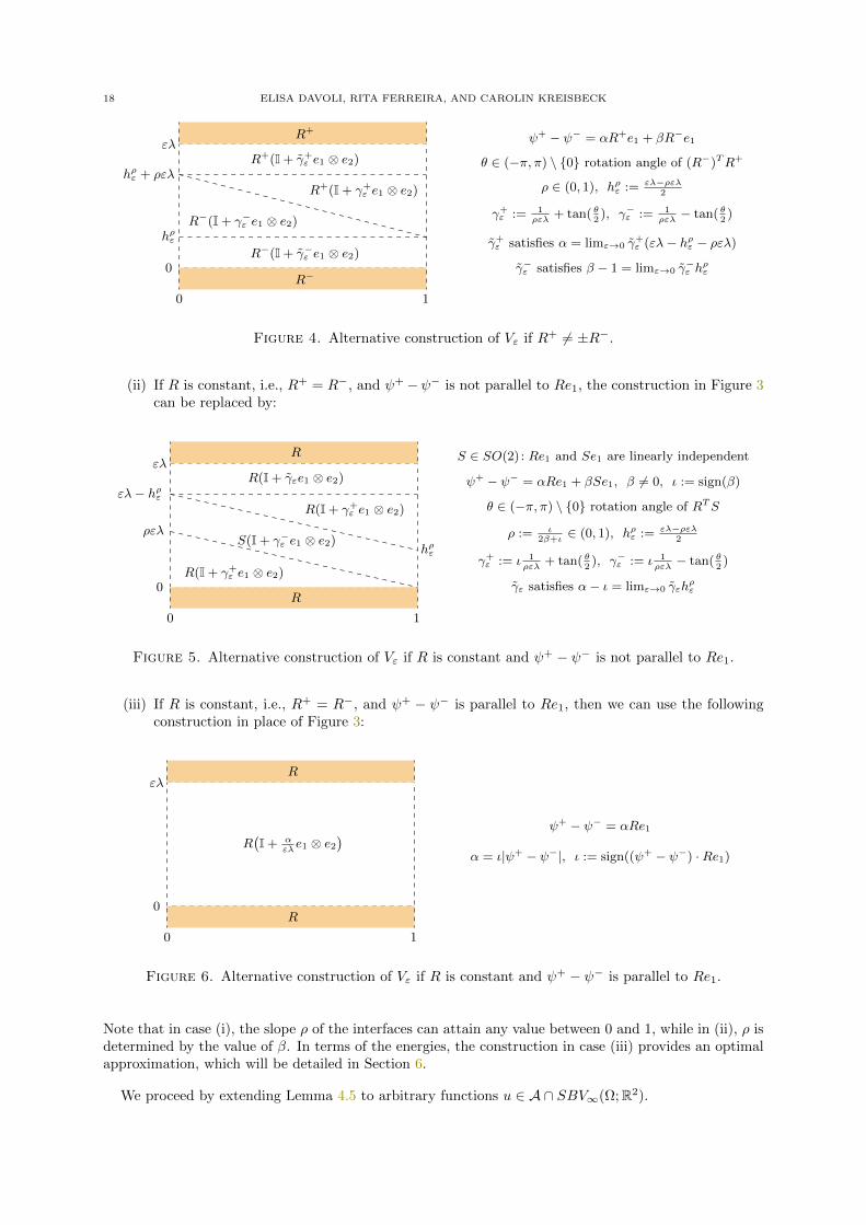
18 ELISA DAVOLI, RITA FERREIRA, AND CAROLIN KREISBECK
0
hρε
hρε + ρελ
ελ
0 1
R−(I + γ−ε e1 ⊗ e2)
R−(I + γ−ε e1 ⊗ e2)
R+(I + γ+ε e1 ⊗ e2)
R+(I + γ+ε e1 ⊗ e2)
R+
R−
ψ+ − ψ− = αR+e1 + βR−e1
θ ∈ (−π, π) \ 0 rotation angle of (R−)TR+
ρ ∈ (0, 1), hρε := ελ−ρελ2
γ+ε := 1
ρελ+ tan( θ
2), γ−ε := 1
ρελ− tan( θ
2)
γ+ε satisfies α = limε→0 γ
+ε (ελ− hρε − ρελ)
γ−ε satisfies β − 1 = limε→0 γ−ε h
ρε
Figure 4. Alternative construction of Vε if R+ 6= ±R−.
(ii) If R is constant, i.e., R+ = R−, and ψ+−ψ− is not parallel to Re1, the construction in Figure 3can be replaced by:
0
ρελ
ελ− hρε
ελ
0 1
hρε
R(I + γ+ε e1 ⊗ e2)
S(I + γ−ε e1 ⊗ e2)
R(I + γ+ε e1 ⊗ e2)
R(I + γεe1 ⊗ e2)
R
R
S ∈ SO(2) : Re1 and Se1 are linearly independent
θ ∈ (−π, π) \ 0 rotation angle of RTS
ψ+ − ψ− = αRe1 + βSe1, β 6= 0, ι := sign(β)
ρ := ι2β+ι
∈ (0, 1), hρε := ελ−ρελ2
γ+ε := ι 1
ρελ+ tan( θ
2), γ−ε := ι 1
ρελ− tan( θ
2)
γε satisfies α− ι = limε→0 γεhρε
Figure 5. Alternative construction of Vε if R is constant and ψ+ − ψ− is not parallel to Re1.
(iii) If R is constant, i.e., R+ = R−, and ψ+ − ψ− is parallel to Re1, then we can use the followingconstruction in place of Figure 3:
0
ελ
0 1
R(I + α
ελe1 ⊗ e2
)
R
R
ψ+ − ψ− = αRe1
α = ι|ψ+ − ψ−|, ι := sign((ψ+ − ψ−) ·Re1)
Figure 6. Alternative construction of Vε if R is constant and ψ+ − ψ− is parallel to Re1.
Note that in case (i), the slope ρ of the interfaces can attain any value between 0 and 1, while in (ii), ρ isdetermined by the value of β. In terms of the energies, the construction in case (iii) provides an optimalapproximation, which will be detailed in Section 6.
We proceed by extending Lemma 4.5 to arbitrary functions u ∈ A ∩ SBV∞(Ω;R2).

HOMOGENIZATION PROBLEMS IN BV 19
Proposition 4.7. Let Ω = (0, 1) × (−1, 1). Then, for every u ∈ A ∩ SBV∞(Ω;R2), there exists a
sequence (uε)ε ⊂ W 1,1(Ω;R2) with∫
Ωuε dx =
∫Ωu dx and uε ∈ Aε for all ε, and such that uε
∗ u in
BV (Ω;R2) or, in other words,
A ∩ SBV∞(Ω;R2) ⊂ A0,
cf. (4.3).
Proof. In view of Remark 4.4 (c), it holds that Ju =⋃`i=1(0, 1) × ai for some ` ∈ N and ai ∈ (−1, 1)
with a1 < a2 < · · · < a`, and setting a0 := −1 and a`+1 := 1, gives
Du =∑
i=0
Ri(I + γe1 ⊗ e2)L2b((0, 1)× (ai, ai+1)
)
+∑
i=1
[(Ri −Ri−1)x1e1 + (Riaie2 + ψ+i −Ri−1aie2 − ψ−i )]⊗ e2H1b
((0, 1)× ai
), (4.25)
where γ ∈ L1(−1, 1), and Ri ∈ SO(2) and ψi ∈ R2 for i = 0, ..., `.We now perform a similar construction as in Lemma 4.5 in a convenient softer layer near each ai,
accounting for the possibility that one or more of the jump lines may not intersect εYsoft ∩ Ω, andreplacing R+ by Ri, R
− by Ri−1, ψ+ by Riaie2 + ψ+i , and ψ− by Ri−1aie2 + ψ−i .
To be precise, fix ε > 0 and i ∈ 1, ..., `. Let Si ∈ SO(2) be such that (i) Si 6∈ Ri−1, Ri; (ii) Sie1
and Rie1 are linearly independent; (iii) θ−i , θ+i ∈ (−π, π) \ 0 are the rotation angles of STi Ri−1 and
STi Ri, respectively. By (ii), there exist αi, βi ∈ R such that
Riaie2 + ψ+i −Ri−1aie2 − ψ−i = αiRie1 + βiSie1. (4.26)
Moreover, we set
γ+ε,i :=
4αiελ
, γε,i :=4βiελ
, µ±ε,i := ± 4
ελ+ tan
(θ±i2
), µ±ε,i := ± 4
ελ− tan
(θ±i2
),
and let κiε ∈ Z be the unique integer such that ai ∈ ε[κiε, κiε+1). Observing that ai 6= aj for i, j ∈ 1, . . . , `with i 6= j and ai ∈ (−1, 1) for all i ∈ 1, . . . , `, we may assume that the sets ε[κiε, κiε + 1)i=1,...,` are
pairwise disjoint, and that⋃`i=1 ε[κ
iε, κ
iε + 1] ⊂ (−1, 1) (this is true for sufficiently small ε > 0). Finally,
with κ0ε := −λ− 1
ε and κ`+1ε := 1
ε , let Vε ∈ L1(Ω;R2×2) be the function defined by
Vε(x) :=
Ri(I + γλ1εYsoft
e1 ⊗ e2) if x ∈ (0, 1)× (ελ+ εκiε, εκi+1ε ) for some i ∈ 0, .., `,
Ri(I + γ+ε,ie1 ⊗ e2) if x ∈ (0, 1)× ( 3ελ
4 + εκiε, ελ+ εκiε) for some i ∈ 1, .., `,Ri(I + µ+
ε,ie1 ⊗ e2) if x1 ∈ (0, 1) and x2 ∈ (− ελ4 x1 + 3ελ4 + εκiε,
3ελ4 + εκiε)
for some i ∈ 1, .., `,Si(I + µ+
ε,ie1 ⊗ e2) if x1 ∈ (0, 1) and x2 ∈ ( ελ2 + εκiε,− ελ4 x1 + 3ελ4 + εκiε)
for some i ∈ 1, .., `,Si(I + γε,ie1 ⊗ e2) if x ∈ (0, 1)× ( ελ4 + εκiε,
ελ2 + εκiε) for some i ∈ 1, .., `,
Si(I + µ−ε,ie1 ⊗ e2) if x1 ∈ (0, 1) and x2 ∈ ( ελ4 x1 + εκiε,ελ4 + εκiε) for some i ∈ 1, .., `,
Ri−1(I + µ−ε,ie1 ⊗ e2) if x1 ∈ (0, 1) and x2 ∈ (εκiε,ελ4 x1 + εκiε) for some i ∈ 1, .., `.
As in the proof of Lemma 4.5, invoking [13, Lemma 3.1] on rank-one connections inMe1 , we find thatVε is a gradient field, meaning that there is uε ∈ W 1,∞(Ω;R2) such that ∇uε = Vε. Adding a suitableconstant allows us to assume that
∫Ωuε dx =
∫Ωu dx. By construction, (uε)ε is a uniformly bounded
sequence in W 1,1(Ω;R2) such that uε ∈ Aε for all ε (see (4.2)). To prove that uε∗ u in BV (Ω;R2), it
suffices to show that
Duε∗ Du in M(Ω;R2×2). (4.27)
The proof of (4.27) follows along the lines of (4.16). For this reason, we only highlight the maindifferences. First, note that the conditions εκ0
ε = −ελ− 1 = −ελ+ a0, εκ`+1ε = 1 = a`+1, and εκiε ≤ ai ≤
ε(κiε + 1) yield
limε→0
εκiε = ai for all i ∈ 0, ..., `+ 1.

20 ELISA DAVOLI, RITA FERREIRA, AND CAROLIN KREISBECK
Hence, 1(0,1)×(ελ+εκiε,εκi+1ε ) → 1(0,1)×(ai,ai+1) and γ1(0,1)×(ελ+εκiε,εκ
i+1ε ) → γ1(0,1)×(ai,ai+1) in L1(Ω) for
i ∈ 0, ..., `+ 1. On the other hand, by the Riemann–Lebesgue lemma, we have 1εYsoft
∗ λ in L∞(R2);
thus,
limε→0
∫
(0,1)×(ελ+εκiε,εκi+1ε )
∇uε(x)ϕ(x) dx = limε→0
∫
Ω
Ri(I + γλ1εYsoft
e1 ⊗ e2)1(0,1)×(ελ+εκiε,εκi+1ε )ϕ(x) dx
=
∫
(0,1)×(ai,ai+1)
Ri(I + γ(x2)e1 ⊗ e2)ϕ(x) dx
for all i ∈ 0, ..., ` and ϕ ∈ C0(Ω). Arguing as in (4.19) with the change of variables z = 4ελ (x2 − εκiε),
leads to
limε→0
∫
(0,1)×(εκiε,ελ4 x1+εκiε)
∇uε(x)ϕ(x) dx
= limε→0
∫ 1
0
∫ ελ4 x1+εκiε
εκiε
Ri−1
(I + tan
( θ−i2
)e1 ⊗ e2 − 4
ελe1 ⊗ e2
)ϕ(x) dx2 dx1
= limε→0
∫ 1
0
∫ x1
0
Ri−1
(ελ4 I + ελ
4 tan( θ−i
2
)e1 ⊗ e2 − e1 ⊗ e2
)ϕ(x1,
ελ4 z + εκiε) dzdx1
= −∫ 1
0
∫ x1
0
Ri−1e1 ⊗ e2ϕ(x1, ai) dzdx1 = −∫ 1
0
Ri−1x1e1 ⊗ e2ϕ(x1, ai) dx1
for all i ∈ 1, ..., ` and ϕ ∈ C0(Ω). Similarly, one can calculate the counterparts to (4.20)–(4.24) in thepresent setting. In view of (4.25) and (4.26), we deduce (4.27), which ends the proof.
Remark 4.8 (On the construction in Proposition 4.7). We observe that the sequence of Lipschitzfunctions (uε)ε constructed in Proposition 4.7 to approximate a given u ∈ A∩SBV∞(Ω;R2) is such that
limε→0
∫
Ω
|∇uε| dx ∼ |Du|(Ω) + 2`.
In other words, the asymptotic behavior of the total variation of (uε)ε incorporates a positive term thatis proportional to the number of jumps of the limit function. This fact prevents us from bootstrappingthe argument in Proposition 4.7 to generalize it to an arbitrary function in A ∩ SBV (Ω;R2).
An analogous statement to Proposition 4.7 holds in A‖.
Proposition 4.9. Let Ω = (0, 1)× (−1, 1). If u ∈ A‖, then there exists a sequence (uε)ε ⊂W 1,1(Ω;R2)
such that uε ∈ Aε for all ε and uε∗ u in BV (Ω;R2); that is,
A‖ ⊂ A0.
Proof. Let u ∈ A‖. Based on (1.13) and (2.4), we can split u into u = v + w, where
v(x) := Rx+ ϑa(x2)Re1 + c and w(x) := ϑs(x2)Re1 for x ∈ Ω, (4.28)
with R ∈ SO(2), c ∈ R2, ϑa ∈ W 1,1(−1, 1), and ϑs ∈ BV (−1, 1) such that ϑ′s = 0. By construction, wehave that v ∈W 1,1(Ω;R2) with ∇v(x) = R(I + ϑ′a(x2)e1 ⊗ e2).
For every ε > 0, let vε ∈W 1,1(Ω;R2) be the function satisfying∫
Ωvε dx =
∫Ωv dx and
∇vε(x) = R(I +
ϑ′a(x2)
λ1εYsoft
(x)e1 ⊗ e2
). (4.29)
By the Riemann–Lebesgue lemma,
vε v in W 1,1(Ω;R2×2). (4.30)
On the other hand, applying Lemma 3.3 to ϑs, we can find a sequence (ϑε)ε ⊂ W 1,∞(−1, 1) such
that ϑε∗→ ϑs in BV (−1, 1) and ϑ′ε = 0 on εIrig ∩ (−1, 1). Then, setting wε(x) := ϑε(x2)Re1 +
∫Ω
(w −ϑε(x2)Re1) dx yields
∇wε(x) = ϑ′ε(x2)Re1 ⊗ e2 = ϑ′ε(x2)1εYsoftRe1 ⊗ e2 (4.31)

HOMOGENIZATION PROBLEMS IN BV 21
and
wε∗→ w in BV (Ω;R2). (4.32)
We define the maps uε := vε + wε in W 1,1(Ω;R2) for every ε,and infer from (4.29) and (4.31) that
∇uε = R(I + γεe1 ⊗ e2
),
where γε(x) :=(ϑ′a(x2)
λ + ϑ′ε(x2))1εYsoft
(x) is a function in L1(Ω) satisfying γε = 0 in εYrig ∩ Ω. Inparticular, uε ∈ Aε for all ε.
Combining (4.30) and (4.32) shows that uε∗ v + w = u in BV (Ω;R2), which finishes the proof.
Finally, we prove Theorem 1.3.
Proof of Theorem 1.3. In view of the discussion in Section 2.4, it suffices to prove the statement on arectangle of the form (cΩ, dΩ) × (aΩ, bΩ), where we recall (1.1) and (1.2). A simple modification of theproofs of Propositions 4.3, 4.7, and 4.9 shows that these results hold for any such rectangles, from whichTheorem 1.3 follows.
5. A lower bound on the homogenized energy
In this section, we present partial results for the homogenization problem for layered composites withrigid components discussed in the Introduction. More precisely, we establish a lower bound estimate onthe asymptotic behavior of the sequence of energies (Eε)ε (see (1.7)), and highlight the main difficultiesin the construction of matching upper bounds. Note that the following analysis is restricted to the cases = e1.
As a start, we first give alternative representations for the involved energies, which will be useful inthe sequel.
Remark 5.1 (Equivalent formulations for Eε and E). In view of the definition of Aε (see (1.6)),it is straightforward to check that the functional Eε in (1.7) satisfies
Eε(u) =
∫
Ω
√|∂2u|2 − 1 dx if u ∈ Aε,
∞ otherwise,=
∫
Ω
√|∇u|2 − 2 det∇u dx if u ∈ Aε,
∞ otherwise,
for u ∈ L10(Ω;R2). Similarly, according to Proposition 4.1, the functional E from (1.10) can be expressed
as
E(u) =
∫
Ω
|γ| dx+ |Dsu|(Ω) if u ∈ A,
∞ otherwise,
for u ∈ L10(Ω;R2).
We can now provide a bound from below on Γ-lim infε→0Eε and prove Theorem 1.2.
Proof of Theorem 1.2. For clarity, we subdivide the proof into two steps. In the first one, we establish thecompactness property. In the second step, we provide two alternative proofs of (1.12). The first proof isbased on a Reshetnyak’s lower semicontinuity result, while the second version is more elementary, relyingon the weak∗ lower semicontinuity of the total variation of a measure. Either of the arguments highlightsa different feature of the representation of A.
Step 1: Compactness. Assume that (uε)ε ⊂ L10(Ω;R2) is such that supεEε(uε) <∞. Then, uε ∈ Aε and
supε ‖∇uε‖L1(Ω;R2×2) < ∞. Hence, using the Poincare–Wirtinger inequality, there exist a subsequence
(uεj )j∈N and u ∈ L10(Ω;R2) ∩ BV (Ω;R2) such that uεj
∗ u in BV (Ω;R2). By Proposition 4.3, we
conclude that u ∈ L10(Ω;R2) ∩ A.
Step 2: Lower bound. Let (uε)ε ⊂ L10(Ω;R2) and u ∈ L1
0(Ω;R2) be such that uε → u in L1(Ω;R2). Wewant to show that
lim infε→0
Eε(uε) ≥ E(u). (5.1)

22 ELISA DAVOLI, RITA FERREIRA, AND CAROLIN KREISBECK
To prove (5.1), one may assume without loss of generality that the limit inferior on the right-hand sideof (5.1) is actually a limit and that this limit is finite. Then, uε ∈ Aε and Eε(uε) < C for all ε, where
C > 0 is a constant independent of ε. Hence, by Step 1, uε∗ u in BV (Ω;R2) and u ∈ A.
Step 2a: Version I. We observe that the map R2×2 3 F 7→√|F |2 − 2 detF is convex (see [18]) and one-
homogeneous. Consequently, it follows from Remark 5.1 and Reshetnyak’s lower semicontinuity theorem(see [2, Theorem 2.38]), under consideration of our notation for the polar decomposition Du = gu|Du|introduced in Section 2.2, that
lim infε→0
Eε(uε) = lim infε→0
∫
Ω
√|∇uε|2 − 2 det∇uε dx ≥
∫
Ω
√|gu|2 − 2 det gu d|Du|. (5.2)
Since ∇u = R(I + γe1 ⊗ e2) with R ∈ BV (Ω;SO(2)) and (Dsu)e1 = 0 (see (4.5)), we have |∇u|2 −2 det∇u = |γ|2 for L2-a.e. in Ω and det gu = 0 for |Dsu|-a.e. in Ω. Thus,
∫
Ω
√|gu|2 − 2 det gu d|Du|
=
∫
Ω
√|∇u|2 − 2 det∇u dx+
∫
Ω
√|gu|2 − 2 det gu d|Dsu|
=
∫
Ω
|γ| dx+ |Dsu|(Ω) = E(u),
(5.3)
where we also used that the relation |gu| = 1 holds |Dsu|-a.e. in Ω.From (5.2) and (5.3), we deduce (5.1).
Step 2b: Version II. By the definition of Aε and (4.1),
∇uε = Rε + γεRεe1 ⊗ e2
with Rε ∈ L∞(Ω;SO(2)) and γε ∈ L1(Ω). Since |γεRεe1 ⊗ e2| = |γε| due to |Rεe1| = 1, the estimateEε(uε) =
∫Ω|γε| dx < C implies that (γεRεe1 ⊗ e2)ε is uniformly bounded in L1(Ω;R2×2). Hence, after
extracting a subsequence if necessary (not relabeled),(γεRεe1 ⊗ e2
)L2bΩ ∗
ν in M(Ω;R2×2)
for some ν ∈ M(Ω;R2×2). Note further that the convergence ∇uεL2bΩ ∗ Du in M(Ω;R2×2) along
with (4.5) yields also Rε∗ R in L∞(Ω;R2×2), where R ∈ L∞(Ω;SO(2)) satisfies in particular that
(∇u)e1 = Re1. Hence, we have
ν = Du−RL2bΩ = (γRe1 ⊗ e2)L2bΩ + Dsu,
where the last equality follows again from (4.5), and by the lower semicontinuity of the total variation,
lim infε→0
Eε(uε) = lim infε→0
∫
Ω
|γε| dx = lim infε→0
∫
Ω
|γεRεe1 ⊗ e2| dx
≥ |ν|(Ω) =
∫
Ω
|γRe1 ⊗ e2| dx+ |Dsu|(Ω) =
∫
Ω
|γ| dx+ |Dsu|(Ω) = E(u).
Remark 5.2 (Discussion regarding optimality of the lower bound). (a) The lower bound (1.12)is optimal in A ∩W 1,1(Ω;R2) ∩ L1
0(Ω;R2) and, more generally (cf. also Remark 4.4), in the set A‖ ∩L1
0(Ω;R2) introduced in (1.13). Precisely, we have
Γ(L1)- limε→0
Eε(u) = E(u) (5.4)
for all u ∈ A‖ ∩ L10(Ω;R2). In view of (1.12), the proof of (5.4) is directly related to the ability to
construct a recovery sequence. We detail two alternative constructions for u ∈ A‖ in Section 6 below.For illustration, we treat here the simpler special case where u ∈ A ∩W 1,1(Ω;R2) ∩ L1
0(Ω;R2).If u ∈ A ∩W 1,1(Ω;R2) ∩ L1
0(Ω;R2), then ∇u = R(I + γe1 ⊗ e2) for some R ∈ SO(2) and γ ∈ L1(Ω)such that ∂1γ = 0 (see Remark 4.4 (a)). As in the proof of Proposition 4.9, we take (uε)ε ⊂W 1,1(Ω;R2)∩L1
0(Ω;R2) such that ∇uε = R(I + γλ1εYsoft
e1 ⊗ e2) for all ε. Then, by the Riemann–Lebesgue lemma,
uε∗ u in BV (Ω;R2) and limε→0Eε(uε) = E(u).(b) The question whether (5.4) holds for a larger class than A‖ is open at this point. We observe
that the gradient-based constructions in Lemma 4.5, Remark 4.6 (i)–(ii), and Proposition 4.7 yield upper

HOMOGENIZATION PROBLEMS IN BV 23
bounds on the Γ- lim sup, which, however, do not match the lower bound of Theorem 1.2. This indicatesthat, in general, a more tailored approach will be necessary.
(c) The upper bounds on the Γ- lim sup of (Eε)ε resulting from Lemma 4.5, Remark 4.6 (i)–(ii),and Proposition 4.7 can be quantified. As previously mentioned, the constructions in Remark 4.6 (iii)and Proposition 4.9 are even recovery sequences. This is not the case for the general construction inLemma 4.5 and for those highlighted in Remark 4.6 (i)–(ii). In the following, we suppose that u ∈A ∩ SBV∞(Ω;R2) ∩ L1
0(Ω;R2) has a single jump as in the statement of Lemma 4.5; i.e.,
u(x) = 1(0,1)×(0,1)(x)(R+(x2)x+ ψ+(x2)) + 1(0,1)×(−1,0)(x)(R−(x2)x+ ψ−(x2))
with R± ∈ SO(2) and ψ± ∈ R2. Then,
E(u) =
∫ 1
0
|(R+ −R−)e1x1 + (ψ+ − ψ−)| dx1,
which can be estimated from above by
E(u) ≤ |R+e1 −R−e1|∫ 1
0
x1 dx1 + |ψ+ − ψ−| ≤ 1 + |ψ+ − ψ−|. (5.5)
For the sequence (uε)ε constructed in Lemma 4.5 (and Lemma 4.7), we obtain, recalling (4.13), that
limε→0
Eε(uε) = |α|+ |β|+ 2 > |α|+ |β|+ 1 ≥ E(u).
Regarding the construction of (uε)ε in Remark 4.6 (i), it follows that
limε→0
Eε(uε) = |α|+ |β − 1|+ 1.
This limit is strictly greater than E(u) as we will show next. If |β − 1| > |β| (i.e., if β < 12 ), this is an
immediate consequence of (5.5). For 12 ≤ β < 1, we use that ψ+ − ψ− = αR+e1 + βR−e1 yields
E(u) ≤∫ 1
0
|x1 + α| dx1 +
∫ β
0
(β − x1) dx1 +
∫ 1
β
(x1 − β) dx1 ≤ 1 + |α|+ β(β − 1) < 1 + |α|+ |β − 1|.
If β ≥ 1, we note that limε→0Eε(uε) = |α| + β, and subdivide the estimate of E(u) into three cases.Recalling the assumption R+ 6= ±R−, we set c := R+e1 ·R−e1 ∈ (−1, 1) to obtain
E(u) =
∫ 1
0
√(x1 + α)2 + (β − x1)2 + 2c(x1 + α)(β − x1) dx1.
Then, we have for α ≥ 0 that
E(u) <
∫ 1
0
√(x1 + α)2 + (β − x1)2 + 2(x1 + α)(β − x1) dx1 = |α+ β| ≤ |α|+ β,
for α ≤ −1 that
E(u) <
∫ 1
0
√(x1 + α)2 + (β − x1)2 − 2(x1 + α)(β − x1) dx1 =
∫ 1
0
(−2x1 − α+ β) dx1
= −1− α+ β < −α+ β = |α|+ β,
and for −1 < α < 0 that
E(u) <
∫ −α
0
(−2x1 − α+ β) dx1 +
∫ 1
−α|α+ β| dx1 = α+ β + α2 < −α+ β = |α|+ β.
Summing up, we have shown that in the context of Remark 4.6 (i),
limε→0
Eε(uε) > E(u).
Finally, we consider the sequence (uε)ε constructed in Remark 4.6 (ii). Then,
limε→0
Eε(uε) = |α− ι|+ |β|+ 1,
and since R+ = R− in this case,
E(u) =√α2 + β2 + 2αβRe1 · Se1.
Using the fact that Re1 · Se1 ∈ (−1, 1), it can be checked that, also here, we have
limε→0
Eε(uε) > E(u).

24 ELISA DAVOLI, RITA FERREIRA, AND CAROLIN KREISBECK
6. Homogenization of the regularized problem
This section is devoted to the proof of our main Γ-convergence result, Theorem 1.4. We first provide analternative characterization of the classA‖ of restricted asymptotically admissible deformations introducedin (1.13).
Lemma 6.1. Let Ω = (0, 1)× (−1, 1). Then, A‖ as in (1.13) admits the representation
A‖ = u ∈ BV (Ω;R2) : ∇u = R(I + γe1 ⊗ e2) with R ∈ SO(2), γ ∈ L1(Ω) such that ∂1γ = 0,
Dsu = (%⊗ e2)|Dsu| with % ∈ L1|Dsu|(Ω;R2) such that (6.1)
|%| = 1 and %||Re1 for |Dsu|-a.e. in Ω.
Proof. Let A‖ denote the set on the right-hand side of (6.1). Arguing as in the beginning of the proofof Proposition 4.9 (precisely, with the notation of (1.13), we set γ(x) = ϑ′a(x2) for x ∈ Ω, and observethat (Dsu)e2 = L1b(0, 1)⊗DsϑsRe1) and exploiting the polar decomposition of measures (cf. (2.2) and
(2.3)) gives rise to A‖ ⊂ A‖. Conversely, the inclusion A‖ ⊂ A, which follows from (4.5), along with (4.6)
yields that A‖ ⊂ A‖.
We are now in a position to prove the Γ-convergence of the energies (Eεδ )ε in (1.14) as ε→ 0.
Proof of Theorem 1.4. As before in the proofs of Theorems 1.1 and 1.3, one may assume without loss ofgenerality that Ω = (0, 1)× (−1, 1). We proceed in three steps.
Step 1: Compactness. Let (uε)ε ⊂ W 1,1(Ω;R2) ∩ L10(Ω;R2) be a sequence such that Eδε (uε) ≤ C for all
ε > 0. Then, because uε ∈ Aε for all ε,
∇uε = Rε(I + γεe1 ⊗ e2) ∈ L1(Ω;R2×2), (6.2)
and ‖γε‖L1(Ω) ≤ C for every ε > 0. Additionally, since each map Rε takes value in the set of proper
rotations, it holds that ‖Rε‖2L∞(Ω;R2×2) = 2 for all ε > 0. Consequently, along with the Poincare-Wirtinger
inequality,
‖uε‖W 1,1(Ω;R2) ≤ C.We further know that ‖∂1uε‖pW 1,p(Ω;R2) = ‖Rεe1‖pW 1,p(Ω;R2) ≤ C/δ for any ε. Thus, after extracting
subsequences if necessary, one can find u ∈ BV (Ω;R2), γ ∈M(Ω), and R ∈W 1,p(Ω;R2×2) such that
uε∗ u in BV (Ω;R2), (6.3)
γεL2 ∗ γ in M(Ω),
Rε R in W 1,p(Ω;R2×2). (6.4)
Recalling the compact embedding W 1,p(Ω) →→ C0,α(Ω) for some 0 < α < 1− 2p , it follows even that
R ∈W 1,p(Ω;SO(2)) ∩ C0,α(Ω;R2×2) and
Rε → R in L∞(Ω;R2×2). (6.5)
As a consequence of Proposition 4.3, it holds that u ∈ A. From Proposition 4.1 and Alberti’s rankone theorem (cf. Section 2.1), we can further infer that R ∈ SO(2), γ ∈ L1(Ω) with ∂1γ = 0, and thatDu satisfies
∇u = R(I + γe1 ⊗ e2) and Dsu = (%⊗ e2)|Dsu|, (6.6)
where % ∈ L|Dsu|(Ω;R2) with |%| = 1 for |Dsu|-a.e. in Ω. To conclude that u ∈ A‖, in view of Lemma 6.1,it remains to show that
%||Re1 |Dsu|-a.e. in Ω. (6.7)
To prove (6.7), we first observe that for every ε, the identity (∇uε)e2 = Rεe2 + γεRεe1, which followsfrom uε ∈ Aε, yields
∫
Ω
[(∇uε)e2 ·Rεe2 − 1]ϕ dx = 0 (6.8)

HOMOGENIZATION PROBLEMS IN BV 25
for all ϕ ∈ C∞c (Ω). Thus, by (6.3) and (6.5) in combination with a weak-strong convergence argument,taking the limit ε→ 0 in (6.8) leads to
∫
Ω
ϕ dx =
∫
Ω
ϕRe2 · d((Du)e2) =
∫
Ω
ϕRe2 · (∇u)e2 dx+
∫
Ω
ϕRe2 · d((Dsu)e2)
for every ϕ ∈ C∞c (Ω). Next, we plug in the identities (∇u)e2 = Re2 + γRe1 and (Dsu)e2 = %|Dsu| (see(6.6)) to derive that
0 =
∫
Ω
ϕRe2 · d((Dsu)e2) =
∫
Ω
ϕRe2 · % d|Dsu|
for every ϕ ∈ C∞c (Ω), which completes the proof of (6.7).
Step 2: Lower bound. Let (uε) ⊂ L10(Ω;R2) and u ∈ L1
0(Ω;R2) be such that uε → u in L1(Ω;R2). Wewant to show that
Eδ(u) ≤ lim infε→0
Eδε (uε). (6.9)
To prove (6.9), we proceed as in the proof of (5.1), observing in addition that
lim infε→0
δ‖∂1uε‖pW 1,p(Ω;R2) = lim infε→0
δ‖Rεe1‖pW 1,p(Ω;R2) ≥ δ‖Re1‖pW 1,p(Ω;R2) = δ|Ω|
due to (6.2) and (6.4) with R ∈ SO(2).
Step 3: Upper bound. Let u ∈ L10(Ω;R2)∩A‖. We want to show that there is a sequence (uε) ⊂ L1
0(Ω;R2)such that uε → u in L1(Ω;R2), and
Eδ(u) ≥ lim supε→0
Eδε (uε). (6.10)
Let (uε)ε ⊂W 1,1(Ω;R2)∩L10(Ω;R2) be the sequence constructed in the proof of Proposition 4.9, that
is, uε ∈ Aε for every ε with
∇uε(x) = R(I +
(ϑ′a(x2)
λ+ ϑ′ε(x2)
)1εYsoft
(x)e1 ⊗ e2
),
where (ϑε)ε ⊂W 1,∞(−1, 1) satisfies
limε→0
∫ 1
−1
|ϑ′ε| dx2 = |Dsϑs|(−1, 1) = |Dsu|(Ω),
and uε∗ u in BV (Ω;R2). Recalling that ϑ′ = ϑ′a + ϑ′s = ϑ′a, we have
lim supε→0
Eδε (uε) ≤ limε→0
(∫
Ω
|ϑ′a(x2)|λ
1εYsoft(x) dx+
∫ 1
−1
|ϑ′ε(x2)| dx2 + δ‖Re1‖pW 1,p(Ω;R2)
)
=
∫
Ω
|ϑ′(x2)| dx+ |Dsu|(Ω) + δ|Ω| = Eδ(u),
which proves (6.10) and completes the proof of the theorem.
Remark 6.2 (On compensated compacteness). We point out that if uε ∈ Aε, with ∇uε = Rε(I +
γεe1 ⊗ e2) for Rε ∈ L∞(Ω;SO(2)) and γε ∈ L1(Ω) with γε = 0 on εYrig ∩ Ω, is such that uε∗ u in
BV (Ω;R2), and if in addition,
Rε → R in C(Ω;R2×2),
then a weak-strong convergence argument implies that
γεL2bΩ =[(∇uε)e2 ·Rεe1
]L2bΩ ∗
(Du)e2 ·Re1 in M(Ω).
However, if continuity and uniform convergence of Rε fail, the limit representation above may nolonger be true in general, even if R ∈ C(Ω;SO(2)). To see this, let us consider the basic construction inRemark 4.6 (ii). In this case,
γεL2bΩ ∗ (α+ β)H1b
((0, 1)× 0
)in M(Ω), (6.11)
whereas
(Du)e2 ·Re1 = [(ψ+ − ψ−) ·Re1]H1b((0, 1)× 0
). (6.12)
Recalling that ψ+ − ψ− = αRe1 + βSe1, the quantities in (6.11) and (6.12) can only match if Re1||Se1,which contradicts the assumption that Re1 and Se1 are linearly independent.

26 ELISA DAVOLI, RITA FERREIRA, AND CAROLIN KREISBECK
The role of the higher-order regularization in (1.14) is exactly that it helps overcome the issue discussedabove. In fact, it guarantees the desired compactness properties for sequences of deformations withequibounded energies.
To conclude, we present an alternative construction for the recovery sequence in Step 3 of the proofof Theorem 1.4.
Alternative proof of Theorem 1.4. As before, we may assume without loss of generality that Ω = (0, 1)×(−1, 1). Moreover, the compactness property and lower bound can be studied exactly as in the proof ofTheorem 1.4 above.
We are then left to show that given u ∈ L10(Ω;R2) ∩ A‖, there exists a sequence (uε)ε ⊂ L1
0(Ω;R2)satisfying uε → u in L1(Ω;R2) and (6.10). We will proceed in three steps, building up complexity.
Step 1. We assume first that u ∈ L10(Ω;R2) ∩ A‖ is an SBV -function with a single, constant jump line
at x2 = 0.This case can be treated as highlighted in Remark 4.6 (iii). Let R ∈ SO(2), γ ∈ L1(Ω) with ∂1γ = 0,
and ψ+, ψ− ∈ R2 with (ψ+ − ψ−)||Re1 be such that
Du = R(I + γe1 ⊗ e2)L2bΩ + (ψ+ − ψ−)⊗ e2H1b((0, 1)× 0).Note that setting ι := sign((ψ+ − ψ−) ·Re1) ∈ ±1, we have ψ+ − ψ− = ι|ψ+ − ψ−|Re1 and
|Du|(Ω) = |Dau|(Ω)|+ |Dsu|(Ω)| = |Dau|(Ω) + |Dju|(Ω) =
∫
Ω
|R(I + γe1 ⊗ e2)| dx+ |ψ+ − ψ−|.
For each ε > 0, set τε := ι |Dju|(Ω)λε = ι |ψ
+−ψ−|λε . Arguing as, for instance, in the proof of Lemma 4.5,
we can find uε ∈ L10(Ω;R2) ∩ Aε such that
∇uε =
R(I + τεe1 ⊗ e2) if x ∈ (0, 1)× (0, λε),
R(I + γλ1εYsoft∩Ωe1 ⊗ e2) otherwise,
and uε∗ u in BV (Ω;R2). Next, we show that this construction yields convergence of energies. Indeed,
we have
limε→0
Eδε (uε) = limε→0
(∫
(0,1)×(0,λε)
|τε| dx+
∫
Ω\(0,1)×(0,λε)
∣∣∣γλ
∣∣∣1εYsoftdx+ δ‖Re1‖pW 1,p(Ω;R2)
)
= |ψ+ − ψ−|+∫
Ω
|γ| dx+ δ|Ω| = |Dsu|(Ω) +
∫
Ω
|γ| dx+ δ|Ω| = Eδ(u).
Step 2. We assume next that u ∈ L10(Ω;R2) ∩A‖ is an SBV -function with a finite number of horizontal
jump lines and with constant upper and lower approximate limits on each jump line.
In this setting, ∇u = R(I+ γe1⊗ e2) with R ∈ SO(2) and γ ∈ L1(Ω) with ∂1γ = 0, Ju =⋃`i=1(0, 1)×
ai with ` ∈ N and −1 < a1 < a2 < · · · < a` < 1, Dju =∑`i=1(ψ+
i − ψ−i ) ⊗ e2H1b((0, 1) × ai) with
ψ±i ∈ R2 satisfying (ψ+i − ψ−i )||Re1 for all i ∈ 1, ..., `, and Dcu = 0. Hence,
Du = R(I + γe1 ⊗ e2)L2bΩ +∑
i=1
(ψ+i − ψ−i )⊗ e2H1b((0, 1)× ai) (6.13)
and
|Dsu|(Ω) =∑
i=1
|ψ+i − ψ−i |.
As in the proof of Proposition 4.7, the idea is to perform a construction similar to that in Step 1around each jump line but accounting for the possibility that one or more of the jump lines may notintersect εYsoft ∩ Ω.
Fix i ∈ 1, ..., ` and ε > 0, and let κiε ∈ Z be the integer such that ai ∈ ε[κiε, κiε + 1). Since ai 6= aj ifi 6= j, we may assume that the sets ε[κiε, κiε + 1)i are pairwise disjoint for all ε > 0 (this is true for allε > 0 sufficiently small). Then, we take uε ∈ L1
0(Ω;R2) ∩ Aε such that
∇uε =
R(I + τ iεe1 ⊗ e2) in (0, 1)× ε(κiε, κiε + λ),
R(I + γλ1εYsoft∩Ωe1 ⊗ e2) otherwise,

HOMOGENIZATION PROBLEMS IN BV 27
where τ iε = ιi|ψ+i −ψ
−i |
λε with ιi := sign((ψ+i − ψ−i ) ·Re1) ∈ ±1. As in the proof of Proposition 4.7, we
obtain that
limε→0
∫
Ω
∇uεϕ dx =∑
i=1
∫ 1
0
ιi|ψ+i − ψ−i |(Re1 ⊗ e2)ϕ(x1, ai) dx1 +
∫
Ω
R(I + γe1 ⊗ e2)ϕ dx (6.14)
for all ϕ ∈ C0(Ω). Recalling (6.13) and the equalities ψ+i −ψ−i = ιi|ψ+
i −ψ−i |Re1 for i ∈ 1, ..., `, (6.14)
shows that Duε∗ Du in M(Ω;R2×2). Hence, uε
∗ u in BV (Ω;R2).
Finally, proceeding exactly as in Step 1, we conclude that this construction also yields convergence ofthe energies. This ends Step 2.
Step 3. We consider now the general case u ∈ L10(Ω;R2) ∩ A‖.
Similarly to the beginning of the proof of Proposition 4.9 (see (4.28)), we can write
u(x) = x1Re1 + φa(x2) + φs(x2), x ∈ Ω,
where φa(x2) := x2Re2 + ϑa(x2)Re1 + c and φs(x2) := ϑs(x2)Re1. Note that φa ∈ W 1,1(−1, 1;R2) andφs ∈ BV (−1, 1;R2) is the sum of a jump function and a Cantor function; in particular, ϑ′ = ϑ′a andDφs = Dsφs (see (2.4)). Moreover,
∇u = Re1 ⊗ e1 +∇φa ⊗ e2 = R(I + ϑ′ae1 ⊗ e2) = R(I + ϑ′e1 ⊗ e2),
Dsu = L1b(0, 1)⊗Dφs,|Dsu|bΩ = L1b(0, 1)⊗|Dφs|.
(6.15)
By Lemma 6.1, there exists % ∈ L1|Dsu|(−1, 1;R2) with |%| = 1 such that
Dsu = (%⊗ e2)|Dsu| and % = (% ·Re1)Re1. (6.16)
Let %h ∈ C∞([−1, 1]) be such that
limh→∞
∫
Ω
|%h(x2)− %(x2)| d|Dsu|(x) = 0. (6.17)
Since |%| = 1, we can choose such a sequence so that |%h| ≤ 1.Due to the properties of good representatives (see [2, (3.24)]) and [19, Lemma 3.2], for each n ∈ N,
there exists a piecewise constant function φn ∈ BV (−1, 1;R2), of the form
φn =
`n∑
i=0
bni χAni ,
where `n ∈ N, (bni )`ni=0 ⊂ R2, and (Ani )`ni=0 is a partition of (−1, 1) into intervals with supAni = inf Ani+1,satisfying
Jφn =
`n⋃
i=1
ani with ani := supAni−1,
limn→∞
‖φn − φs‖L1(−1,1;R2) = 0, (6.18)
limn→∞
|Dφn|(−1, 1) = limn→∞
|Djφn|(−1, 1) = |Dφs|(−1, 1) = |Dsu|(Ω). (6.19)
Indeed, (6.18) and (6.19) mean that (φn)n∈N converges strictly to φs in BV (−1, 1;R2), which impliesthat
|Dφn| ∗ |Dφs| in M(−1, 1), (6.20)
see [2, Proposition 3.5].Finally, for n ∈ N, we define
un(x) := x1Re1 + φa(x2) + φn(x2) + cn, x ∈ Ω,
where cn ∈ R2 are constants chosen so that∫
Ωun dx = 0. Note that cn → 0 as n → ∞ by (6.18).
Moreover, for each n ∈ N, the map un ∈ L10(Ω;R2) has the same structure as in Step 2 apart from the
condition (u+n − u−n )||Re1 on Jun , which a priori is not satisfied. Choosing ιni := %h(ani ) · Re1, we can
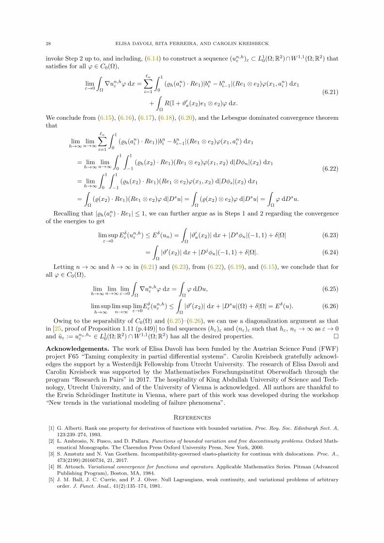
28 ELISA DAVOLI, RITA FERREIRA, AND CAROLIN KREISBECK
invoke Step 2 up to, and including, (6.14) to construct a sequence (un,hε )ε ⊂ L10(Ω;R2)∩W 1,1(Ω;R2) that
satisfies for all ϕ ∈ C0(Ω),
limε→0
∫
Ω
∇un,hε ϕ dx =
`n∑
i=1
∫ 1
0
(%h(ani ) ·Re1)|bni − bni−1|(Re1 ⊗ e2)ϕ(x1, ani ) dx1
+
∫
Ω
R(I + ϑ′a(x2)e1 ⊗ e2)ϕ dx.
(6.21)
We conclude from (6.15), (6.16), (6.17), (6.18), (6.20), and the Lebesgue dominated convergence theoremthat
limh→∞
limn→∞
`n∑
i=1
∫ 1
0
(%h(ani ) ·Re1)|bni − bni−1|(Re1 ⊗ e2)ϕ(x1, ani ) dx1
= limh→∞
limn→∞
∫ 1
0
∫ 1
−1
(%h(x2) ·Re1)(Re1 ⊗ e2)ϕ(x1, x2) d|Dφn|(x2) dx1
= limh→∞
∫ 1
0
∫ 1
−1
(%h(x2) ·Re1)(Re1 ⊗ e2)ϕ(x1, x2) d|Dφs|(x2) dx1
=
∫
Ω
(%(x2) ·Re1)(Re1 ⊗ e2)ϕ d|Dsu| =∫
Ω
(%(x2)⊗ e2)ϕ d|Dsu| =∫
Ω
ϕ dDsu.
(6.22)
Recalling that |%h(ani ) ·Re1| ≤ 1, we can further argue as in Steps 1 and 2 regarding the convergenceof the energies to get
lim supε→0
Eδε (un,hε ) ≤ Eδ(un) =
∫
Ω
|ϑ′a(x2)| dx+ |Dsφn|(−1, 1) + δ|Ω| (6.23)
=
∫
Ω
|ϑ′(x2)| dx+ |Djφn|(−1, 1) + δ|Ω|. (6.24)
Letting n→∞ and h→∞ in (6.21) and (6.23), from (6.22), (6.19), and (6.15), we conclude that forall ϕ ∈ C0(Ω),
limh→∞
limn→∞
limε→0
∫
Ω
∇un,hε ϕ dx =
∫
Ω
ϕ dDu, (6.25)
lim suph→∞
lim supn→∞
limε→0
Eδε (un,hε ) ≤∫
Ω
|ϑ′(x2)| dx+ |Dsu|(Ω) + δ|Ω| = Eδ(u). (6.26)
Owing to the separability of C0(Ω) and (6.25)–(6.26), we can use a diagonalization argument as thatin [25, proof of Proposition 1.11 (p.449)] to find sequences (hε)ε and (nε)ε such that hε, nε →∞ as ε→ 0and uε := unε,hεε ∈ L1
0(Ω;R2) ∩W 1,1(Ω;R2) has all the desired properties.
Acknowledgements. The work of Elisa Davoli has been funded by the Austrian Science Fund (FWF)project F65 “Taming complexity in partial differential systems”. Carolin Kreisbeck gratefully acknowl-edges the support by a Westerdijk Fellowship from Utrecht University. The research of Elisa Davoli andCarolin Kreisbeck was supported by the Mathematisches Forschungsinstitut Oberwolfach through theprogram “Research in Pairs” in 2017. The hospitality of King Abdullah University of Science and Tech-nology, Utrecht University, and of the University of Vienna is acknowledged. All authors are thankful tothe Erwin Schrodinger Institute in Vienna, where part of this work was developed during the workshop“New trends in the variational modeling of failure phenomena”.
References
[1] G. Alberti. Rank one property for derivatives of functions with bounded variation. Proc. Roy. Soc. Edinburgh Sect. A,
123:239–274, 1993.[2] L. Ambrosio, N. Fusco, and D. Pallara. Functions of bounded variation and free discontinuity problems. Oxford Math-
ematical Monographs. The Clarendon Press Oxford University Press, New York, 2000.
[3] S. Amstutz and N. Van Goethem. Incompatibility-governed elasto-plasticity for continua with dislocations. Proc. A.,473(2199):20160734, 21, 2017.
[4] H. Attouch. Variational convergence for functions and operators. Applicable Mathematics Series. Pitman (Advanced
Publishing Program), Boston, MA, 1984.[5] J. M. Ball, J. C. Currie, and P. J. Olver. Null Lagrangians, weak continuity, and variational problems of arbitrary
order. J. Funct. Anal., 41(2):135–174, 1981.

HOMOGENIZATION PROBLEMS IN BV 29
[6] A. C. Barroso, J. Matias, M. Morandotti, and D. R. Owen. Second-order structured deformations: relaxation, integral
representation and applications. Arch. Ration. Mech. Anal., 225(3):1025–1072, 2017.
[7] B. Benesova, M. Kruzık, and A. Schlomerkemper. A note on locking materials and gradient polyconvexity. Math.Models Methods Appl. Sci., 28(12):2367–2401, 2018.
[8] A. Braides. Gamma-convergence for beginners. Number 22 in Oxford lecture series in mathematics and its applications.Oxford University Press, Oxford, 1. ed edition, 2005.
[9] A. Chambolle, A. Giacomini, and M. Ponsiglione. Piecewise rigidity. J. Funct. Anal., 244:134–153, 2007.
[10] R. Choksi, G. Del Piero, I. Fonseca, and D. Owen. Structured deformations as energy minimizers in models of fractureand hysteresis. Math. Mech. Solids, 4(3):321–356, 1999.
[11] R. Choksi and I. Fonseca. Bulk and interfacial energy densities for structured deformations of continua. Arch. Rational
Mech. Anal., 138(1):37–103, 1997.[12] F. Christowiak. Homogenization of layered materials with stiff components. PhD thesis, Universitat Regensburg, 2012.
[13] F. Christowiak and C. Kreisbeck. Homogenization of layered materials with rigid components in single-slip finite crystal
plasticity. Calc. Var. Partial Differential Equations, 56(3):Art. 75, 28pp, 2017.[14] F. Christowiak and C. Kreisbeck. Asymptotic rigidity of layered structures and its application in homogenization
theory. Preprint arXiv:1808.10494, 2018.
[15] S. Conti. Relaxation of single-slip single-crystal plasticity with linear hardening. In P. Gumbsch, editor, MultiscaleMaterials Modeling, pages 30–35. Fraunhofer IRB, Freiburg, 2006.
[16] S. Conti, G. Dolzmann, and C. Kreisbeck. Asymptotic behavior of crystal plasticity with one slip system in the limit
of rigid elasticity. SIAM Journal on Mathematical Analysis, 43(5):2337–2353, 2011.[17] S. Conti, G. Dolzmann, and C. Kreisbeck. Relaxation of a model in finite plasticity with two slip systems. Math. Models
Methods Appl. Sci., 23(11):2111–2128, 2013.[18] S. Conti and F. Theil. Single-slip elastoplastic microstructures. Arch. Ration. Mech. Anal., 178(1):125–148, 2005.
[19] G. Crasta and V. De Cicco. A chain rule formula in the space BV and applications to conservation laws. SIAM J.
Math. Anal., 43(1):430–456, 2011.[20] G. Dal Maso. An introduction to gamma-convergence. Number 8 in Progress in nonlinear differential equations and
their applications. Birkhauser, Boston, 1993.
[21] G. Dal Maso, I. Fonseca, G. Leoni, and M. Morini. Higher-order quasiconvexity reduces to quasiconvexity. Arch. Ration.Mech. Anal., 171(1):55–81, 2004.
[22] E. Davoli and G. Francfort. A critical revisiting of finite elastoplasticity. SIAM Journal of Mathematical Analysis,
47:526–565, 2015.[23] E. Davoli and M. Friedrich. Two-well rigidity and multidimensional sharp-interface limits for solid-solid phase transi-
tions. arXiv:1810.06298, 2018.
[24] G. Del Piero and D. R. Owen. Structured deformations of continua. Arch. Rational Mech. Anal., 124(2):99–155, 1993.[25] R. Ferreira and I. Fonseca. Characterization of the multiscale limit associated with bounded sequences in BV . J.
Convex Anal., 19(2):403–452, 2012.[26] I. Fonseca, G. Leoni, and J. Maly. Weak continuity and lower semicontinuity results for determinants. Arch. Ration.
Mech. Anal., 178(3):411–448, 2005.
[27] M. Friedrich and M. Kruzık. On the passage from nonlinear to linearized viscoelasticity. SIAM J. Math. Anal.,50(4):4426–4456, 2018.
[28] M. Giaquinta and D. Mucci. Maps of bounded variation with values into a manifold: total variation and relaxed energy.
Pure Appl. Math. Q., 3(2, Special Issue: In honor of Leon Simon. Part 1):513–538, 2007.[29] D. Grandi and U. Stefanelli. Finite plasticity in PTP . Part I: Constitutive model. Continuum Mech. Thermodyn,
29:97–116, 2017.
[30] D. Grandi and U. Stefanelli. Finite plasticity in PTP . Part II: Quasi-Static Evolution and Linearization. SIAM J.Math. Anal., 49:1356–1384, 2017.
[31] R. Hill. The mathematical theory of plasticity. Clarendon Press, Oxford, 1950.
[32] D. Idczak. The generalization of the Du Bois-Reymond lemma for functions of two variables to the case of partialderivatives of any order. Banach Center Publications, 35:221–236, 1996.
[33] E. H. Lee. Elastic-plastic deformation at finite strains. J. Appl. Mech., 36:1–6, 1969.[34] A. Mielke. Finite elastoplasticity, lie groups and geodesics on SL(d). In Geometry, Dynamics, and Mechanics, pages
61–90. Springer, New York, 2002.
[35] A. Mielke. Energetic formulation of multiplicative elastoplasticity using dissipation distances. Contin. Mech. Thermo-dyn., 15:351–382, 2003.
[36] A. Mielke and T. Roubıcek. Rate-independent elastoplasticity at finite strains and its numerical approximation. Math.
Models Methods Appl. Sci., 26(12):2203–2236, 2016.[37] P. Naghdi. A critical review of the state of finite plasticity. Z. Angew. Math. Phys., 41:315–394, 1990.
[38] P. Podio-Guidugli. Contact interactions, stress, and material symmetry, for nonsimple elastic materials. Theoret. Appl.
Mech., 28/29:261–276, 2002.[39] R. Toupin. Elastic materials with couple stresses. Arch. Ration. Mech. Anal., 11:385–414, 1962.
[40] R. Toupin. Theory of elasticity with couple stress. Arch. Ration. Mech. Anal., 17:85–112, 1964.
30 ELISA DAVOLI, RITA FERREIRA, AND CAROLIN KREISBECK
University of Vienna, Faculty of Mathematics, Oskar-Morgenstern-Platz 1, 1090 Vienna, Austria
E-mail address: [email protected]
King Abdullah University of Science and Technology (KAUST), CEMSE Division, Thuwal 23955-6900, Saudi
Arabia
E-mail address: [email protected]
Mathematisch Instituut, Universiteit Utrecht, Postbus 80010, 3508 TA Utrecht, The Netherlands
E-mail address: [email protected]

Chapter 2
Wulff-shape emergence in
crystallization problems
This chapter consists of the following papers:
1) E. Davoli, P. Piovano, U. Stefanelli.
Wulff shape emergence in graphene.
Math. Models Methods Appl. Sci. 26 (2016), 2277–2310.
2) E. Davoli, P. Piovano, U. Stefanelli.
Sharp N3/4 law for minimizers of the edge-isoperimetric problem on the triangular
lattice.
Journal of Nonlinear Science, 27 (2017), 627–660.


October 14, 2016 8:37 WSPC/103-M3AS 1650053
Mathematical Models and Methods in Applied SciencesVol. 26, No. 12 (2016) 2277–2310c⃝ World Scientific Publishing CompanyDOI: 10.1142/S0218202516500536
Wulff shape emergence in graphene
Elisa Davoli∗ and Paolo Piovano†
Faculty of Mathematics, University of Vienna,Oskar-Morgenstern-Platz 1,
A-1090 Vienna, Austria∗[email protected]
Ulisse Stefanelli
Faculty of Mathematics, University of Vienna,Oskar-Morgenstern-Platz 1,
A-1090 Vienna, Austria
Istituto di Matematica Applicata e TecnologieInformatiche “E. Magenes” — CNR,Via Ferrata 1, I-27100 Pavia, Italy
Received 22 January 2016Accepted 16 July 2016
Published 4 October 2016Communicated by F. Brezzi
Graphene samples are identified as minimizers of configurational energies featuring bothtwo- and three-body atomic-interaction terms. This variational viewpoint allows for adetailed description of ground-state geometries as connected subsets of a regular hexa-gonal lattice. We investigate here how these geometries evolve as the number n of carbonatoms in the graphene sample increases. By means of an equivalent characterization ofminimality via a discrete isoperimetric inequality, we prove that ground states convergeto the ideal hexagonal Wulff shape as n → ∞. Precisely, ground states deviate from suchhexagonal Wulff shape by at most Kn3/4 + o(n3/4) atoms, where both the constant Kand the rate n3/4 are sharp.
Keywords: Ground state; hexagonal lattice; isoperimetric inequality; Wulff shape.
AMS Subject Classification: 82D25
1. Introduction
The recent realization of high crystalline quality graphene samples at room tem-
perature can be regarded as a breakthrough in materials science and has led to
the attribution of the 2010 Nobel Prize in physics to Geim and Novoselov. The
fascinating electronic and mechanical properties of single-atom-thick carbon sur-
faces are believed to offer unprecedented opportunities for innovative applications,
2277

October 14, 2016 8:37 WSPC/103-M3AS 1650053
2278 E. Davoli, P. Piovano & U. Stefanelli
ranging from next-generation electronics to pharmacology, and including batteries
and solar cells. New findings are emerging at an always increasing pace and involve
thousands of researchers worldwide cutting across materials science, physics, and
chemistry, extending from fundamental science to novel applications.
The stand of the mathematical understanding of graphene is comparably less
developed. All available results are extremely recent and concern the modeling
of transport properties of electrons in graphene sheets,3,6,11,14,23,33,34 homogeniza-
tion,7,32 atomistic-to-continuum passage for nanotubes,12 geometry of monolayers
under Gaussian perturbations,10 external charges25 or magnetic fields,9 combina-
torial description of graphene patches,20 and numerical simulation of dynamics
via nonlocal elasticity theory.43 Remarkably, the determination of the equilibrium
shapes and the Wulff shapes of graphene samples and graphene nanostructures is
still a challenging problem.1,5,17
Graphene ideally corresponds to a regular, two-dimensional, hexagonal arrange-
ment of carbon atoms. In the bulk of a graphene sample each carbon atom is cova-
lently bonded to three neighbors. These covalent bonds are of sp2-hybridized type
and ideally form 2π/3 angles in a plane. In order to describe these bonds, some
phenomenological interaction energies, including two- and three-body interaction
terms, have been presented and partially validated.37,38 The arrangement of car-
bon atoms in the two-dimensional crystal emerges then as the global effect of the
combination of local atomic interactions, and can be seen as the result of a geome-
tric optimization process: by identifying the configuration of n carbon atoms with
their positions x1, . . . , xn ⊂ R2, one minimizes a given configurational energy
E : R2n → R ∪ ∞ and proves that the minimizers are indeed subsets of a regular
hexagonal lattice. The configurational energies for carbon feature a decomposition
E = E2 + E3 where E2 corresponds to an attractive–repulsive two-body interac-
tion, favoring some preferred spacing of the atoms, and E3 encodes three-body
interactions, expressing the specific geometry of sp2-covalent bonding in carbon.
The above-variational viewpoint brings the study of graphene geometries into
the realm of the so-called crystallization problems. A first analysis in this direction is
in Ref. 24, where E2 is assumed to be of Lennard-Jones type and E3 favors 2π/3 and
4π/3 bond angles. The focus of Ref. 24 is on the thermodynamic limit: as n → ∞ the
minimal energy density is proven to converge to a finite value, corresponding indeed
to the configuration in which the atoms arrange themselves in a suitably stretched
hexagonal lattice. Analogous thermodynamic-limit results are obtained in Ref. 13,
where nonetheless the term E2 favors π bond angles. The crystallization problem
for a finite number of carbon atoms is studied in Ref. 31 where the periodicity
of ground states as well as the exact quantification of the ground-state energy is
obtained, together with the discussion of carbon nanostructures such as fullerenes
and nanotubes, see also Refs. 27, 28, 31. The reader is referred to Refs. 18, 40
and 41 for one-dimensional crystallization results, to Refs. 22, 35, 39 and 42 for
the two-dimensional case either in the finite and in the thermodynamic-limit case,
and to Refs. 29 and 30 for crystallization in the square lattice. Results on the
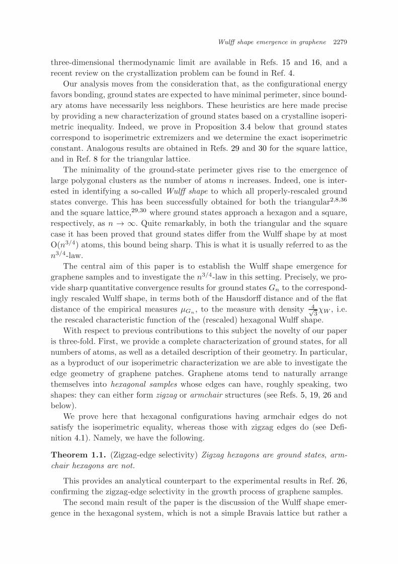
October 14, 2016 8:37 WSPC/103-M3AS 1650053
Wulff shape emergence in graphene 2279
three-dimensional thermodynamic limit are available in Refs. 15 and 16, and a
recent review on the crystallization problem can be found in Ref. 4.
Our analysis moves from the consideration that, as the configurational energy
favors bonding, ground states are expected to have minimal perimeter, since bound-
ary atoms have necessarily less neighbors. These heuristics are here made precise
by providing a new characterization of ground states based on a crystalline isoperi-
metric inequality. Indeed, we prove in Proposition 3.4 below that ground states
correspond to isoperimetric extremizers and we determine the exact isoperimetric
constant. Analogous results are obtained in Refs. 29 and 30 for the square lattice,
and in Ref. 8 for the triangular lattice.
The minimality of the ground-state perimeter gives rise to the emergence of
large polygonal clusters as the number of atoms n increases. Indeed, one is inter-
ested in identifying a so-called Wulff shape to which all properly-rescaled ground
states converge. This has been successfully obtained for both the triangular2,8,36
and the square lattice,29,30 where ground states approach a hexagon and a square,
respectively, as n → ∞. Quite remarkably, in both the triangular and the square
case it has been proved that ground states differ from the Wulff shape by at most
O(n3/4) atoms, this bound being sharp. This is what it is usually referred to as the
n3/4-law.
The central aim of this paper is to establish the Wulff shape emergence for
graphene samples and to investigate the n3/4-law in this setting. Precisely, we pro-
vide sharp quantitative convergence results for ground states Gn to the correspond-
ingly rescaled Wulff shape, in terms both of the Hausdorff distance and of the flat
distance of the empirical measures µGn , to the measure with density 4√3χW , i.e.
the rescaled characteristic function of the (rescaled) hexagonal Wulff shape.
With respect to previous contributions to this subject the novelty of our paper
is three-fold. First, we provide a complete characterization of ground states, for all
numbers of atoms, as well as a detailed description of their geometry. In particular,
as a byproduct of our isoperimetric characterization we are able to investigate the
edge geometry of graphene patches. Graphene atoms tend to naturally arrange
themselves into hexagonal samples whose edges can have, roughly speaking, two
shapes: they can either form zigzag or armchair structures (see Refs. 5, 19, 26 and
below).
We prove here that hexagonal configurations having armchair edges do not
satisfy the isoperimetric equality, whereas those with zigzag edges do (see Defi-
nition 4.1). Namely, we have the following.
Theorem 1.1. (Zigzag-edge selectivity) Zigzag hexagons are ground states, arm-
chair hexagons are not.
This provides an analytical counterpart to the experimental results in Ref. 26,
confirming the zigzag-edge selectivity in the growth process of graphene samples.
The second main result of the paper is the discussion of the Wulff shape emer-
gence in the hexagonal system, which is not a simple Bravais lattice but rather a

October 14, 2016 8:37 WSPC/103-M3AS 1650053
2280 E. Davoli, P. Piovano & U. Stefanelli
so-called multilattice. We relate the Wulff shape emergence with the isoperimetric
nature of ground states. Our result reads as follows.
Theorem 1.2. (Emergence of the Wulff shape) Let Gn be a sequence of ground
states in the hexagonal lattice. Let Wn be the zigzag hexagon centered in the origin
and with side rn (see (1.6) below). Then, there exists a suitable translation G′n of
Gn such that
|G′n\Wn| ≤ Kn3/4 + o(n3/4), (1.1)
where | · | is the cardinality of the set, and
K :=27/4
31/4. (1.2)
In addition, there holds:
dH(G′n, Wn) ≤ O(n1/4),
∥µG′n
− µWn∥ ≤ Kn−1/4 + o(n−1/4), (1.3)
∥µG′n
− µWn∥F ≤ Kn−1/4 + o(n−1/4), (1.4)
µG′n
∗ 4√3χW weakly* in the sense of measures,
and ∥∥∥∥µG′n
− 4√3χW
∥∥∥∥F
≤ 2Kn−1/4 + o(n−1/4), (1.5)
where dH is the Hausdorff distance, ∥ · ∥ is the total variation, and ∥ · ∥F is the flat
norm (see (2.4)).
Our third main result concerns the sharpness of the n3/4-law (1.1). We show
not only the sharpness of the convergence ratio, but also of the constant K in front
of the leading term. We have the following.
Theorem 1.3. (Sharpness of the n3/4-law) There exists a sequence of integers nj
such that for every sequence of ground states Gnj properties (1.1), (1.3) and (1.4)
hold with equalities.
Our proof strategy differs from that of Refs. 29 and 36, as it is not based on
configuration rearrangements. The argument here moves from the control of the
radius rGn of the maximal hexagon HGn contained in a ground state Gn with n
atoms. In particular, we define
rn := minrGn :Gn is a ground state with n atoms, (1.6)
and we show that every ground state (up to translation) consists of the n-Wulff
shape Wn with comparably few extra atoms, see Sec. 6. Precisely, we prove a delicate
estimate of the form rn ∼ n1/2 which entails that the atoms of Gn which do not
belong to Wn are at most O(n3/4). An outcome of our proof is that the convergence

October 14, 2016 8:37 WSPC/103-M3AS 1650053
Wulff shape emergence in graphene 2281
rates and the constants above are sharp. Indeed, we explicitly construct a sequence
of integers such that every corresponding sequence of ground states attains the
right-hand sides of (1.1), (1.3) and (1.4).
In the triangular lattice, the existence of a sequence of ground states whose
deviation from the Wulff shape is exactly of order n3/4 was exhibited in Ref. 36 with
no specific control on the convergence constants. With a different implementation
of the method discussed here, we revisited the triangular-lattice case in Ref. 8,
obtaining explicit, sharp convergence constants.
The paper is organized as follows. In Sec. 2, we introduce some notation and a
few definitions. In Sec. 3, we highlight the isoperimetric nature of ground states.
Section 4 contains a discussion of the equilibrium shapes of graphene samples, and
a proof of the fact that armchair hexagons are not ground states. In particular, we
prove there Theorem 1.1. In Sec. 5, we provide delicate lower and upper bounds for
rn. Section 6 is eventually devoted to the proofs of Theorems 1.2 and 1.3.
2. Notation and Setting of the Problem
Let the hexagonal lattice be given by
L := mt1 + nt2 + cw : m, n ∈ Z, c ∈ 0, 1,
with
t1 :=
(√3
0
), t2 :=
(√3/2
3/2
), and w :=
(0
1
).
Note that the minimal distance between points in L is 1 (see Fig. 1).
We denote a configuration of n atoms by Cn := x1, . . . , xn ∈ R2n, the distance
between two atoms, xi and xj , by ℓij , and the counterclockwise-oriented angle
between the two segments xi −xj and xk −xj by θijk. The energy of a configuration
Cn is defined as
E(Cn) := E2(Cn) + E3(Cn) =1
2
∑
i=j
v2(ℓij) +∑
(i,j,k)∈Av3(θijk), (2.1)
where v2 : [0, ∞) → [−1, ∞] and v3 : [0, 2π] → [0, ∞) are the two-body and the
three-body interaction potentials. We notice that the energy is invariant under
rotations and translations. Two atoms xi and xj are said to be bonded, or there
is an (active) bond between xi and xj , if 1 ≤ ℓij <√
2. The index set A in (2.1)
Fig. 1. An example of a subset of L.

October 14, 2016 8:37 WSPC/103-M3AS 1650053
2282 E. Davoli, P. Piovano & U. Stefanelli
is defined as the set of all triples (i, j, k) for which the angle θijk separates two
active bonds. We will always assume that v2(1) = −1 and that v2(ℓ) vanishes for
ℓ ≥√
2 (see below). We work under the assumption that v3 reaches its minimum
value only at the angles π/3 and 2π/3, and that ground states are subsets of the
hexagonal lattice. We use the standard notation for the right- and left-continuous
integer-parts: ⌊x⌋ :=maxz ∈ Z : z≤x and ⌈x⌉ :=minz ∈ Z : x≤z, respectively.
Under suitable assumptions on the potentials v2 and v3, it was established in
Ref. 31 that all ground-state configurations are (isometric to) subsets of the hexa-
gonal lattice L and that the value of the energy for every ground state with n
atoms is given by
en := −⌊
3n
2−√
3n
2
⌋. (2.2)
From this point on all configurations are hence seen as subsets of L.
The bond graph of a configuration Cn is the graph consisting of all its vertices
and active bonds. For every atom xi ∈ Cn, we indicate by b(xi) the number of
active bonds of Cn with an endpoint in xi. Denoting by B(Cn) the total number
of bonds in Cn, there holds
B(Cn) =1
2
n∑
i=1
b(xi).
A configuration Cn is said to be connected if for every two atoms y1, y2 ∈ Cn
there exists a collection of atoms x1, . . . , xi ∈ Cn such that y1 is bonded to x1, xi
is bonded to y2, and every atom xj , with 2 ≤ j ≤ i − 1 is bonded both to xj−1 and
to xj+1. We call minimal simple cycles of a configuration all the simple cycles in
the graph that are hexagons of side 1.
The area A(Cn) of a configuration Cn is given by the number of minimal simple
cycles of Cn. Denoting by F (Cn) ⊂ R2 the closure of the union of the regions
enclosed by the minimal simple cycles of Cn, and by G(Cn) ⊂ R2 the union of all
bonds which are not included in F (Cn), the perimeter P of a configuration Cn is
defined as
P (Cn) := H1(∂F (Cn)) + 2H1(G(Cn)),
where H1 is the one-dimensional Hausdorff measure. As already observed in Ref. 29,
there holds
P (Cn) = limε0
H1(∂(∂F (Cn) ∪ G(Cn) + Bε)),
where Bε = y ∈ R2 | |y| ≤ ε.
With a slight abuse of notation, the symbol | · | will denote, according to the
context, both the absolute value of a real number and the cardinality of a set.
We will often use the notion of edge boundary Θ of a configuration with respect
to a reference lattice: this is the union of unit segments in the reference lattice that

October 14, 2016 8:37 WSPC/103-M3AS 1650053
Wulff shape emergence in graphene 2283
are not included in the graph of Cn but share one and only one endpoint with Cn,
Θ(Cn) :=(x, y) ∈ (L)2 : x ∈ Cn, y /∈ Cn
.
The edge perimeter of a configuration Cn will be defined as the number of segments
belonging to its edge boundary.
For every configuration Cn := x1, . . . , xn in L, we denote by µCn the empirical
measure associated to the rescaled configuration x1/√
n, . . . , xn/√
n, that is,
µCn :=1
n
∑
i
δxi/√
n. (2.3)
Given a Lebesgue measurable set A ⊂ R2, we will designate by L2(A) its two-
dimensional Lebesgue measure. For any bounded Radon measure µ, the symbol
∥µ∥ will represent its total variation in R2, whereas ∥µ∥F will be the flat norm of
µ, defined as
∥µ∥F := sup
∫
R2
ϕ dµ : ϕ is Lipschitz with ∥ϕ∥W 1,∞(R2) ≤ 1
. (2.4)
The set of bounded Radon measures on R2 will be denoted by Mb(R2).
3. Discrete Isoperimetric Inequality
In this section, we prove that connected configurations satisfy a discrete isoperi-
metric inequality, and we characterize ground states as configurations realizing the
isoperimetric equality. We first deduce some preliminary relations between the area,
the perimeter, the edge perimeter, and the energy of configurations. Let Cn be a
configuration. Then
E(Cn) = −B(Cn) = −1
2
n∑
i=1
b(xi).
Since every atom in L has exactly three bonds, we have
|Θ(Cn)| =
n∑
i=1
(3 − b(xi)), (3.1)
and the energy and the edge perimeter of configurations are related by
E(Cn) = −3
2n +
1
2|Θ(Cn)|. (3.2)
Recalling that every minimal simple cycle of Cn consists of six bonds, we have
6A(Cn) = 2B(Cn ∩ F (Cn)) − B(Cn ∩ ∂F (Cn))
= −2E(Cn ∩ F (Cn)) − H1(∂F (Cn)).
On the other hand,
H1(G(Cn)) = B(Cn ∩ G(Cn)) = −E(Cn ∩ G(Cn)).

October 14, 2016 8:37 WSPC/103-M3AS 1650053
2284 E. Davoli, P. Piovano & U. Stefanelli
Hence, we obtain
P (Cn) = H1(∂F (Cn)) + 2H1(G(Cn))
= −2E(Cn ∩ F (Cn)) − 6A(Cn) − 2E(Cn ∩ G(Cn))
= −2E(Cn) − 6A(Cn),
that is
E(Cn) = −3A(Cn) − 1
2P (Cn). (3.3)
In conclusion, we can express the energy of a hexagonal configuration Cn as a
linear combination of its area and its perimeter. Likewise, in view of (3.2), the edge
perimeter satisfies
|Θ(Cn)| = 3n − 6A(Cn) − P (Cn).
The following result is a direct corollary of Theorem 7.3 (p. 142) in Ref. 21.
Proposition 3.1. There exists a total order τ : N → L such that for all n ∈N the configuration Dn defined by Dn := xτ(1), . . . , xτ(n) (which we call daisy)
minimizes E over all configurations with n atoms, i.e.
E(Dn) = minCn⊂L
E(Cn) = en, (3.4)
where en is the quantity defined in (2.2).
The total order in Proposition 3.1 is nonunique. For the sake of definiteness we
fix here our attention on a specific order τ , as described in Ref. 31. For n = 6k2,
k ∈ N, the sequence D6k2 is defined inductively as follows: D6 is a minimal simple
cycle in L, and D24 is obtained by externally attaching to all bonds of D6 another
hexagon. D6k2 is then defined recursively (see Fig. 2).
1 2
3
4
6
1 2
3
45 5
6
7
8 9
1011
Fig. 2. The daisies D6 and D24 and the total order τ .

October 14, 2016 8:37 WSPC/103-M3AS 1650053
Wulff shape emergence in graphene 2285
For k, m ∈ N, and 0 < m < 12k(k+1), D6k2+m is constructed as in the proof of
Proposition 5.1 (Step 1) in Ref. 31. In view of Proposition 3.1, it is always possible
to add one atom to a daisy Dn so that the new configuration with n + 1 points is
still a ground state.
To every configuration Cn ⊂ L, we associate a weight function
∆Cn : Cn → 0, 1, 2,
defined as
∆Cn(x) := |y ∈ Cn : (x, y) ∈ Cn × Cn, y <τ x|,for every x ∈ Cn, and we rewrite Cn as the union
Cn =
2⋃
k=0
Ckn,
where
Ckn := x ∈ Cn :∆Cn(x) = k
for k = 0, . . . , 2. In particular, |C0n| corresponds to the number of connected compo-
nents of Cn.
The next proposition allows us to express the energy, the perimeter, the edge
perimeter, and the area of a configuration Cn as a function of the cardinality of the
sets Ckn .
Proposition 3.2. Let Cn be a configuration in L. Then,
E(Cn) = −|C1n| − 2|C2
n|, (3.5)
A(Cn) = |C2n|, (3.6)
P (Cn) = 2|C1n| − 2|C2
n|, (3.7)
|Θ(Cn)| = 3|C0n| + |C1
n| − |C2n| (3.8)
for every n > 1. Moreover,
E(Cn) = −3A(Cn) − |Θ(Cn)| + 3|C0n|. (3.9)
Proof. We first observe that
E(Cn) = −n∑
i=1
∆Cn(xi).
For i = 0, . . . , n − 1, let Ci be the subset of Cn containing its first i points
according to the total order τ . If xτ(i) ∈ C0n, then
A(Ci) − A(Ci−1) = 0, P (Ci) − P (Ci−1) = 0, |Θ(Ci)| − |Θ(Ci−1)| = 3; (3.10)
if xτ(i) ∈ C1n, then
A(Ci) − A(Ci−1) = 0, P (Ci) − P (Ci−1) = 2, |Θ(Ci)| − |Θ(Ci−1)| = 1; (3.11)

October 14, 2016 8:37 WSPC/103-M3AS 1650053
2286 E. Davoli, P. Piovano & U. Stefanelli
whereas, if xτ(i) ∈ C2n, we have
A(Ci)− A(Ci−1)= 1, P (Ci)− P (Ci−1)= − 2, |Θ(Ci)| − |Θ(Ci−1)| = − 1.
(3.12)
Properties (3.5)–(3.8) follow from (3.10)–(3.12). Claim (3.9) is a direct conse-
quence of (3.3), (3.7) and (3.8).
In view of Proposition 3.2 we obtain the following.
Proposition 3.3. The following assertions are equivalent and hold true for every
connected hexagonal configuration Cn:
(i) |Θ(Dn)| ≤ |Θ(Cn)|;(ii) P (Dn) ≤ P (Cn);
(iii) A(Dn) ≥ A(Cn).
Proof. The first assertion is a direct consequence of (3.2) and (3.4), and is equiva-
lent to (ii) by (3.7) and (3.8). The equivalence between (ii) and (iii) follows by (3.3)
and (3.4).
We are now in a position to characterize connected ground states as extremizers
of a discrete isoperimetric problem.
Proposition 3.4. Every connected configuration Cn satisfies√
A(Cn) ≤ knP (Cn), (3.13)
where
kn :=
√⌊(αn)2 − αn⌋ − n + 1
4(αn)2 − 4⌊(αn)2 − αn⌋ − 6(3.14)
and αn :=√
3n/2.
Moreover, connected ground states correspond to those configurations for which
(3.13) holds with equality, and, equivalently, to those configurations that attain the
maximum area
an := −n + ⌊(αn)2 − αn⌋ + 1,
and the minimum perimeter
pn := 4(αn)2 − 4⌊(αn)2 − αn⌋ − 6.
Proof. We claim that√
A(Dn) = knP (Dn). (3.15)
In fact, in view of (3.5) and Theorem 3.1, there holds
en = E(Dn) = −|D1n| − 2|D2
n|,

October 14, 2016 8:37 WSPC/103-M3AS 1650053
Wulff shape emergence in graphene 2287
whereas by (3.2) and (3.8),
3n + 2en = |Θ(Dn)| = 3 + |D1n| − |D2
n|,
where en is the ground-state energy defined in (2.2). Solving the previous system
of equations we deduce
|D1n| = 2n + en − 2, (3.16)
and
|D2n| = −n − en + 1. (3.17)
Claim (3.15) follows from (3.6), (3.7), (3.16) and (3.17), by observing that
√A(Dn) =
√|D2
n| =√
−n − en + 1
= kn(6n + 4en − 6) = kn(2|D1n| − 2|D2
n|) = knP (Dn).
Inequality (3.13) is a direct consequence of (3.15) and Proposition 3.3. By Propo-
sition 3.3 and (3.2), connected ground states Gn satisfy
|Θ(Gn)| = en +3
2n
and attain the maximum area and the minimum perimeter. The values of an and
pn follow from (3.8), (3.7) and (3.9).
4. Equilibrium Shapes of Graphene Samples
In this section, we characterize the edge geometry of graphene samples. We first
introduce a few definitions.
Definition 4.1. For every s ∈ N we define the set HZs of zigzag hexagons of side
s as
HZs := D6s2 + q : q ∈ L
(for all s ∈ N, the configuration D6s2 is a complete hexagon of hexagons). For s ∈ N,
s ≥ 3, the set HAs of armchair hexagons of side s is defined as
HAs := As + q : q ∈ L.
In the expression above, A3 is given by the union of D24 with six extra minimal
simple cycles, glued externally to the center of each side of D24 (see Fig. 3). For
s > 3, As is defined recursively by adding an extra armchair layer of minimal simple
cycles to As−1. We point out that the construction is different for s even and s odd
(see Fig. 3).

October 14, 2016 8:37 WSPC/103-M3AS 1650053
2288 E. Davoli, P. Piovano & U. Stefanelli
A5
A4A3
Fig. 3. (Color online) The armchair hexagons A3, A4 and A5. Each armchair hexagon As fors > 3 is obtained by adding a layer of extra minimal simple cycles (in blue) to the correspondingarmchair hexagon As−1 (in yellow). Notice the different structure for s even and for s odd.
4.1. Proof of Theorem 1.1
The optimality of zigzag hexagons follows in view of Definition 4.1 and Proposi-
tion 3.1.
We claim that for every s ∈ N, s ≥ 3, there holds
P (As) > p|As|. (4.1)
Indeed, by the definition of As we have |A3| = 42, and for s > 3:
|As| = |As−1| +
⎧⎨⎩
6(2s − 1) if s is even,
6s if s is odd,
that is
|As| =9
2s2 +
⎧⎪⎨⎪⎩
3s if s is even,
3
2if s is odd.

October 14, 2016 8:37 WSPC/103-M3AS 1650053
Wulff shape emergence in graphene 2289
On the other hand, the perimeter of each armchair hexagon As is given by
P (As) = 12s − 6. (4.2)
For s odd, we have
α|As| =
√3|As|
2=
3
2s
√3 +
1
s2.
Hence,
α2|As| =
9
4(3s2 + 1) ∈ N,
and
α2|As| − ⌊α2
|As| − α|As|⌋ =
⌈3
2s
√3 +
1
s2
⌉.
In view of Proposition 3.4 there holds
p|As| = 4α2|As| − 4⌊α2
|As| − α|As|⌋ − 6 (4.3)
≤ 4
(3
2s
√3 +
1
s2
)− 2 (4.4)
= 6√
3s +6
s(√
3 +√
3 + 1s2
) − 2 (4.5)
< 6√
3s +
√3
s− 2 < 12s − 6 (4.6)
for s ≥ 3.
By combining (4.2) and (4.6) we obtain claim (4.1) for s odd. The result for
s even, s ≥ 4 follows via analogous computations. In view of Proposition 3.4 and
(4.1) armchair hexagons are not extremizers of the isoperimetric inequality, and
hence are not ground states.
5. The Radius of the n-Wulff Shape
For simplicity in what follows we will refer to the elements of HZs as hexagons of
side s, omitting the word zigzag. We first introduce the notion of maximal hexagon
associated to a ground state.
Let Gn be a ground state in the hexagonal lattice L. Let
rGn := maxs ∈ N : there exists a point q ∈ L such that D6s2 + q ⊆ Gn.
For every q ∈ L such that D6r2Gn
+ q ⊂ Gn, we will refer to the set
HGn := D6r2Gn
+ q,

October 14, 2016 8:37 WSPC/103-M3AS 1650053
2290 E. Davoli, P. Piovano & U. Stefanelli
as a maximal hexagon associated to Gn. We recall that
Gn =
2⋃
k=0
Gkn,
where
Gkn := x ∈ Gn : ∆Gn(x) = k.
Let us preliminary check that maximal hexagons are non-degenerate for n > 6.
We recall that the n-Wulff shape Wn is the zigzag hexagon centered in the origin
with side rn (see (1.6)), i.e.
Wn := D6r2n.
Proposition 5.1. The radius rn of the n-Wulff shape Wn (see (1.6) and Theorem
1.2) with n > 6, satisfies rn ≥ 1.
Proof. Let n ∈ N be such that there exists a ground state Gn with rGn = 0. Then
Gn does not contain any set of the form D6 + q with q ∈ L, that is, for every
x ∈ Gn, there holds (see (3.12)):
x /∈ G2n. (5.1)
By (3.11) and (3.12), property (5.1) is equivalent to the claim that every element
of Gn\G0n contributes to the overall perimeter of Gn, and the contribution of each
element is exactly 2. Since we are assuming that Gn is connected (i.e. |G0n| = 1),
this implies that
P (Gn) ≥ 2(n − 1).
By Proposition 3.4 it follows that
4(αn)2 − 4⌊(αn)2 − αn⌋ − 6 = P (Dn) = pn ≥ 2(n − 1),
which in turn implies
n − 1 ≥ ⌊(αn)2 − αn⌋ ≥ (αn)2 − αn,
and finally yields n −√
6n ≤ 0, that is 0 ≤ n ≤ 6.
Fix n ∈ N and let Gn be a connected ground state. We aim at proving an
estimate from below on the radius rGn of HGn in terms of the number n of atoms.
We first introduce some definitions.
Definition 5.1. (Zigzag path) Let ℓ be a line orthogonal to one of the three dia-
meters of a minimal simple cycle of the lattice and intersecting L. The zigzag path
identified by ℓ is the union of points p ∈ L such that either p ∈ ℓ or there exists
a minimal simple cycle H of L such that p belongs to H , and the two atoms in
H bonded to P are in ℓ. Note that each point of a zigzag path divides it into two
half-zigzag paths (see Fig. 5).

October 14, 2016 8:37 WSPC/103-M3AS 1650053
Wulff shape emergence in graphene 2291
Cn Cn
P1
P2
P3P4
P1
P2
P3
P4
Fig. 4. On the left, the points P1, . . . , P4 belong to a side of Cn, on the right the segment joiningP2 and P3 is a corner edge of Cn.
Let P1, . . . , P4 ∈ L ∩ ∂F (Cn) be such that P1 is bonded to P2, and for i = 2, 3
the point Pi is bonded both to Pi−1 and Pi+1. If there exists a unique zigzag path
passing through all the points P1, . . . , P4 we will say that this zigzag path is a side
of Cn. If two different (nonparallel) zigzag paths intersect in the unitary segment
joining P2 and P3 we will refer to this segment as a corner edge of Cn (see Fig. 4).
We will say that Cn has an angle α in a corner edge v (or in a point P ) if the
two lines ℓ1α and ℓ2
α, identifying the sides of Cn and passing through v (respectively,
P ), intersect forming an angle of width α. The choice of α or 2π − α will be clear
P
Q
ℓ
sℓ
v
σ1
σ2
S
ℓ1
ℓ2
) 2π3
Fig. 5. (Color online) On the left, the zigzag path sℓ originated by the line ℓ. On the right, thetwo zigzag paths σ1 and σ2 intersect in the corner edge v, forming an angle 2π/3. The associatedangular sector S is marked in yellow.
October 14, 2016 8:37 WSPC/103-M3AS 1650053
2292 E. Davoli, P. Piovano & U. Stefanelli
from the context. Alternatively, we will say that the zigzag paths associated to ℓ1α
and ℓ2α form an angle α with (or in) v (respectively, P ).
Finally, if S ⊂ L is such that ∂(F (S))∩L (see Sec. 2) is the union of two zigzag
paths forming an angle α, we will call S an angular sector of width α, see Fig. 5.
By Proposition 5.1 we can assume that rGn ≥ 1. Let v0, . . . , v5 be the corner
edges of HGn , where v0 is assumed to be lying on the x-axis (without loss of
generality), and v1, . . . , v5 are numbered counterclockwise starting from v0. For
k = 0, . . . , 4, let sk be the zigzag path joining vk and vk+1, and let s5 be the zigzag
path joining v5 and v0. Let lk be the line identifying the path sk, and denote by νk
the unit normal to lk pointing toward the exterior of HGn . We define
λk := maxj ∈ N : sjk ∩ Gn = 0, (5.2)
where
sjk := sk + jνk
for j ∈ N. Let πk be also the subset of L such that ∂F (πk)= sk and F (πk)∩HGn = ∅.
We show now that ground states satisfy a connectedness property with respect
to zigzag paths.
Definition 5.2. (Hex-connectedness) Let S be a subset of L and let P ∈ L. We
say that P disconnects a zigzag path in S if P /∈ S and there exist Pa, Pb ∈ S such
that Pa and Pb are joined by a zigzag path passing through P .
Let S be a subset of L. We say that S is hex-connected if every P ∈ L disconnects
at most one zigzag path in S.
Notice that from every point P ∈ L there are exactly three nonparallel lines
which depart from P and identify a zigzag path (see Definition 5.1).
Proposition 5.2. Ground states are hex-connected.
Proof. For the sake of contradiction assume that there exists a ground state Gn
which is not hex-connected. Then there exists a point P ∈ L which disconnects two
zigzag paths in Gn. In particular, there exists a line ℓ0 orthogonal to one of the
diameters of a minimal simple cycle of the lattice, and intersecting L, such that
the two half-zigzag paths starting from P and identified by ℓ0 are both intersecting
Gn. Let ℓ1, . . . , ℓm be the lines parallel to ℓ0, intersecting Gn, and such that for
every i = 1, . . . , m, the distance between ℓi and ℓ0 is given by 3ni/2, where ni ∈ N.
For i = 0, . . . , m, let ci be the number of points of Gn contained in the zigzag path
identified by ℓi.
We first rearrange the set ci in a decreasing order, constructing another set
di with the property that d0 ≥ d1 ≥ · · · ≥ dm. Then, we separate the elements
of di having odd indexes from those having even indexes and we consider a new
family fi obtained by first taking into account the elements of di with even
indexes, in decreasing order with respect to their indexes, and then the elements

October 14, 2016 8:37 WSPC/103-M3AS 1650053
Wulff shape emergence in graphene 2293
of di having odd indexes, with increasing order with respect to their indexes. In
particular we define:
fi :=
⎧⎪⎨⎪⎩
dm−2i i = 0, . . . ,m
2
d2i−m−1 i =m
2+ 1, . . . , m
if m is even, and
fi :=
⎧⎪⎪⎨⎪⎪⎩
dm−1−2i i = 0, . . . ,(m − 1)
2
d2i−m i =(m + 1)
2, . . . , m
if m is odd.
The set fi constructed above has the property that its central elements have
the maximum value, and the values of the elements decrease in an alternated way
by moving from the center of fi toward i = 0 and i = m. Let i and i + 1 be the
indexes corresponding to the two central elements of the set fi, if m is odd, and
to the central element of fi and the maximum between its two neighbors, if m
is even. As an example, if we start with a set ci = 3, 4, 7, 8, 2, 2, 8, the family
di is given by 8, 8, 7, 4, 3, 2, 2 and the set fi by 2, 3, 7, 8, 8, 4, 2. Here i = 4.
Fix two points P i, P i+1 ∈ Lh such that the segment P iP i+1 has length one and
is orthogonal to ℓ0. Let σ1 and σ2 be two half-zigzag paths, starting from P i and
P i+1, respectively, forming an angle 2π/3 with P iP i+1, and such that there exists
a convex region S of the plane whose boundary is given by σ1, σ2, and P iP i+1.
Consider the points P0, . . . , P i−1 ∈ σ1, defined as
|P i − Pj | = (i − j)√
3, j = 0, . . . , i − 1.
Analogously, consider the points P i+2, . . . , Pm ∈ σ2, satisfying
|P i+1 − Pj | = (j − i)√
3, j = i + 2, . . . , m.
For j = 0, . . . , m, let ℓj be the line parallel to ℓ0 and passing through Pj . To
construct the set Gn we consider fj consecutive points in S on the zigzag path
identified by each line ℓj , starting from Pj (see Figs. 5 and 6). The set Gn is clearly
hex-connected, the number of bonds in the zigzag paths identified by the lines
parallel to ℓ0 has increased, and the number of bonds between parallel zigzag paths
has not decreased. Hence
E(Gn) < E(Gn),
providing a contradiction to the optimality of the ground state Gn.
As a corollary of Proposition 5.2 it follows that ground states have no vacancies.
Proposition 5.3. Let Gn be a ground state. Then F (Gn) is simply connected.
Proof. By contradiction, if F (Gn) is not simply connected then there exists a point
in L that disconnects three zigzag paths in Gn. Therefore Gn is not hex-connected.

October 14, 2016 8:37 WSPC/103-M3AS 1650053
2294 E. Davoli, P. Piovano & U. Stefanelli
P
ℓ0ℓ1ℓ2 ℓ3 P1
P2
Fig. 6. (Color online) A configuration Cn before (in black) and after (in red) the rearrangementdescribed in Proposition 5.2.
We conclude this overview on connectedness properties of ground states with
the following proposition.
Proposition 5.4. Ground states are connected.
We omit the proof of this result as it follows by adapting the proof of Proposi-
tion 5.2.
In view of Propositions 5.2–5.4, the quantity λk defined in (5.2) provides the
number of nonempty parallel zigzag paths of atoms in Gn ∩ πk. By the definition
of τ , each partially full level of atoms around HGn is characterized by the fact that
the difference between the number of points on the level having weight one and
those having weight two is strictly positive. To be precise,
5∑
k=0
λk ≤ |G1n\HGn | − |G2
n\HGn |.
On the other hand, by (3.11) and (3.12),
|G1n\HGn | − |G2
n\HGn | =P (Gn) − P (HGn)
2=
pn
2− 6rGn + 3,
thus yielding
5∑
k=0
λk ≤ pn
2− 6rGn + 3. (5.3)
Given a ground state Gn and its maximal hexagon HGn := D6r2Gn
+ q, denote
by H+Gn
and H++Gn
the sets H+Gn
:= D6(rGn+1)2 + q, and H++Gn
:= D6(rGn+2)2 + q,
respectively. Denote by v′i and v′′
i , i = 0, . . . , 5, the corner edges of H+Gn
and H++Gn
,
respectively, with the convention that both v′i and v′′
i are parallel to vi. For i =
0, . . . , 5, let V 1i and V 2
i be the two extrema of vi, numbered counterclockwise. Let
(V ′i )1, (V ′
i )2, (V ′′i )1, (V ′′
i )2, s′i and s′′
i be defined accordingly.

October 14, 2016 8:37 WSPC/103-M3AS 1650053
Wulff shape emergence in graphene 2295
In the remaining part of this subsection we provide a characterization of the
geometry of Gn\H+Gn
, by subdividing this set into good polygons Pk and bad poly-
gons Tk, and by showing that the cardinality of Gn\H+Gn
is, roughly speaking, the
same as the one of the union of good polygons.
We first prove that, by the optimality of HGn , there exists a corner edge of H++Gn
which does not intersect Gn.
Proposition 5.5. Let Gn be a ground state, and HGn be its maximal hexagon.
Then there exists a corner edge v′′j of H++
Gn, j = 0, . . . , 5, which does not inter-
sect Gn.
Proof. By the maximality of HGn , there exists a point P ∈ ∂F (H+Gn
) such that
P /∈ Gn.
If P does not disconnect s′i then either v′
i or v′i+1 do not intersect Gn. By the
hex-connectedness of Gn (see Proposition 5.2) then also the corresponding corner
edge of H++Gn
does not intersect Gn, and we obtain the thesis.
Assume now that P disconnects s′i. Since Gn is hex-connected, the point P does
not disconnect any other zigzag path. Therefore there exists an angular sector S
centered in P and of width π/3 such that
S ∩ Gn = ∅. (5.4)
Assume by contradiction that all corner edges of H++Gn
intersect Gn. In view of (5.4),
the set (Gn\HGn)∩πi is subdivided into two components. Denoting them by Γ1 and
Γ2, we have that Γj ∩s1i = ∅ and Γj ∩s2
i = ∅, for j = 1, 2. Without loss of generality
we can assume that Γ1 ∩ sλi
i = ∅. Consider now the set M := Γ1 ∩ (sλi
i ∪ sλi−1i ).
We claim that we can construct a new set Gn, by rearranging the atoms of M and
by leaving the other elements of Gn fixed, such that
E(Gn) < E(Gn). (5.5)
There are three possible scenarios.
Case 1: Γ1 contains at least two points Pa and Pb with the property that for each
of them there is no minimal cycle passing through it and entirely contained in Gn.
We proceed by moving the two points to s1i ∩ (L\Gn) in such a way that Pa is
bonded to Γ2. If possible, we move also Pb to s1i ∩ (L\Gn) so that Pa and Pb are
bonded. If this is not possible because si ∩ (L\Gn) contains only one element, then
we already created an extra bond. With this procedure we lose two bonds when
removing Pa and Pb from Γ1, but we gain at least three bonds when we attach
them to Γ2, therefore the total energy strictly decreases.
Case 2: In Γ1 there exists exactly one point Pa with the property that there is
no minimal cycle containing it and entirely contained in Gn. We argue moving this
single point to s1i ∩ (L\Gn) in such a way that Pa is bonded to Γ2. Afterward, we
move iteratively all the (remaining) points in sλi
i ∩ Γ1 to s1i ∩ (L\Gn) (in the same
way as described in Case 1 for Pb). If after moving Pa there are no remaining points

October 14, 2016 8:37 WSPC/103-M3AS 1650053
2296 E. Davoli, P. Piovano & U. Stefanelli
in sλi
i ∩Γ1, we apply the same rearrangement to sλi−1i ∩Γ1 (note that λi ≥ 2 because
all corner edges of H++Gn
intersect Gn). As a result of the procedure described above,
the energy is strictly decreased. If at any moment during the process of attaching
points to Γ2 we create a bond between Γ1 and Γ2, we stop the rearrangement as
the number of bonds has strictly increased.
Case 3: Every point of Γ1 belongs to a minimal cycle entirely contained in Gn. In
this case we first move all points in sλi
i ∩ Γ1 but one, in the same way as described
in Cases 1 and 2. As a result of this procedure, either we already created an extra
bond (and hence there is nothing left to prove) or we are now in the same situation
described in Case 2. The thesis follows then arguing exactly as in Case 2.
We proceed by showing that for every hexagon of side rGn + 2 there exists an
angular sector of width π/3, and centered in one of its corner edges, which does not
intersect Gn.
Proposition 5.6. Let Gn be a ground state, and HGn be its maximal hexagon.
Then:
(i) There exists a corner edge v′′i of H++
Gn, i =0, . . . , 5, and an angular sector S of
width π/3, centered in (V ′′i )1 or (V ′′
i )2, and such that S ∩ Gn = ∅.(ii) Every hexagon in L with side rGn + 2 has a corner edge and a corresponding
angular sector of width π/3 which do not intersect Gn.
Proof. By Proposition 5.5 we can assume that v′′0 does not intersect Gn. Assume
first that both (V ′′0 )1 and (V ′′
0 )2 do not disconnect any zigzag path. Consider the
two half-zigzag paths in which v′′0 divides s′′
0 . Then at least one of them does not
intersect Gn. Analogously, at least one of the two half-zigzag paths in which v′0
divides s′5 does not intersect Gn. Finally, the two half-zigzag paths, departing from
(V ′0 )1 and (V ′
0)2, not parallel to s0 and s5, and in the opposite direction with respect
to the center of HGn , do not intersect Gn. According to the geometric position of the
four half-zigzag paths identified beforehand, and using again the hex-connectedness
of Gn we obtain (i), the sector S being of width 2π/3. The case in which at least one
between (V ′′0 )1 and (V ′′
0 )2 disconnects one zigzag path (see Proposition 5.2) follows
accordingly, yielding a sector S of width π/3. The proof of (ii) is an adaptation of
the proof of (i).
Without loss of generality, in view of Proposition 5.6 we can assume that v′′0 !
Gn. For k = 2, 3, 4, 5, let π′k be the subset of L such that⎧⎪⎪⎨⎪⎪⎩
π′k = F (π′
k) ∩ L,
∂F (π′k) ∩ L = sλk
k ,
HGn ⊂ π′k.
Consider the set R :=(⋂5
k=0 π′k
)∖H+
Gn.

October 14, 2016 8:37 WSPC/103-M3AS 1650053
Wulff shape emergence in graphene 2297
By construction, Gn ⊂ H+Gn
∪ R, and for every x ∈ R and k = 0, . . . , 5 there
exists
jk ∈[−λ( k+3
6 −⌊ k+36 ⌋) − 2rGn − 2, λk
],
such that x ∈ sjk
k . In particular, every x ∈ R is uniquely determined by a pair of
indexes (jk, jk′), with k′ = k + 3 in Z6.
We subdivide the region R into disjoint polygons as
R =
⎛⎝
5⋃
j=0
Pj
⎞⎠ ∪
⎛⎝
5⋃
j=0
Tj
⎞⎠. (5.6)
For a ∈ [−2(rGn + 1), 2(rGn + 1)], denote by P 1k (a) the subset of L enclosed by s2
k,
sak, s1
k+1, s−rGn
k+1 ; and by P 2k (a) the set delimited by sa
k, sλk
k , sλk−1−rGn
k−1 , sλk−1
k−1 . For
k = 0, . . . , 5, the sets Pk in (5.6) are defined as follows:
Pk :=
⎧⎨⎩
P 1k (λk) ∩ R if λk ≤ λk−1 + 1,
(P 1k (λk − λk−1 + 1) ∩ R) ∪ P 2
k (λk − λk−1 + 1) if λk > λk−1 + 1,
with the convention that λ−1 := λ5. Note that |Pk| = 2(rGn + 1)(λk − 1) for every
k = 0, . . . , 5.
The sets Tk are given, roughly speaking, by the “portions of L” between Pk−1
and Pk. To be precise,
Tk :=x ∈ R : x∈ s
jk−1
k−1 ∩ sjk
k , with 2 ≤ jk−1 ≤λk−1, 2 ≤ jk ≤ λk, jk−1 ≥ jk
and, if λk−1 > λk−2 + 1, jk−1 ≤ jk + λk−1 − λk−2
, (5.7)
see Fig. 7.
We have that
n ≤ |H+Gn
| + |R| − |R\Gn|,where |H+
Gn| = 6(rGn + 1)
2. We observe that
|R| =
5∑
j=0
|Pj | +5∑
j=0
|Tj | = 2(rGn + 1)
5∑
j=0
(λj − 1) +
5∑
j=0
|Tj | − 1.
We proceed now in counting the points in R which do not belong to the ground
state Gn. In particular, we prove a lower bound for such number in terms of the
cardinality of
H := H ⊂ L ∩ (H+Gn
∪ R) : H is a hexagon of side rGn + 2.
Proposition 5.7.
|R\Gn| ≥ 2|H|.
Proof. Set M := |H|. We show by induction on m = 1, . . . , M that for every
family Hm ⊂ H with |Hm| = m, there exists a collection of pairs of bonded atoms

October 14, 2016 8:37 WSPC/103-M3AS 1650053
2298 E. Davoli, P. Piovano & U. Stefanelli
T2 P1
P0
H+Gn
P2
P5
T5
T1
P4T4
P3
T3
T0
Fig. 7. The structure of a ground state Gn. In the figure above, rGn = 3, λ0 = 6, λ1 = 6, λ2 = 4,λ3 = 7, λ4 = 6, and λ5 = 5. The blue shapes outlined in black, the yellow shapes outlined in black,and the green shapes outlined in black correspond to the closed subsets of the plane associated toH+
Gn, to the parallelograms Pj , and to the triangles Tj , respectively.
VHm ⊂ R\Gn with |VHm | = m satisfying the following property: identifying each
segment with its extrema, the correspondence associating to each pair (ν1, ν2) ∈VHm a hexagon H ∈ Hm having a corner edge in (ν1, ν2) is a bijection.
We remark that the thesis will follow once we prove the assertion for m = M . For
m = 1 the claim holds by Proposition 5.6. Assume now that the claim is satisfied for
m = m. Consider a family Hm+1 = H1, . . . , Hm+1 ⊂ H, and the polygon Pm+1 :=⋃m+1i=1 Hi ⊂ R. We subdivide the remaining part of the proof into four steps.
Step 1: There exists a corner edge (ν1, ν2) of Pm+1 such that νi ∈ Pm+1\Gn for
i = 1, 2.

October 14, 2016 8:37 WSPC/103-M3AS 1650053
Wulff shape emergence in graphene 2299
Indeed, assume by contradiction that every corner edge of Pm+1 belongs to Gn.
Then every corner edge of Hm+1 in F (Pm+1) would belong to Gn by Proposition 5.3.
Thus all corner edges of Hm+1 would belong to Gn, contradicting Proposition 5.5.
Step 2: By Proposition 5.6(ii) there exists an angular sector S of width at least
π/3, centered in ν1, ν2, or in (ν1, ν2), and such that S ∩ Gn = ∅. Denote by σ1 and
σ2 the two zigzag paths forming its boundary.
Step 3: We claim that there exists a corner edge (ν1, ν2) of Pm+1 such that
(ν1, ν2) ⊂ Pm+1\Gn, and (ν1, ν2) is associated to an angle 2π/3 of Pm+1.
Observe that Pm+1 can have corner edges with angles 2π/3, 4π/3 or 5π/3. If
the corner edge (ν1, ν2) found in Step 2 is associated to an angle 2π/3, there is
nothing to prove. If (ν1, ν2) corresponds to an angle 4π/3 or 5π/3, then there are
two possible cases:
Case 1: F (S) ∩ Pm+1 = ∅. Then, for every j = 1, 2, there exists νj ∈ σj such
that νj is one of the two extrema of a corner edge of Pm+1 entirely contained in
S, and at least one among the zigzag paths from ν1 to ν1 and from ν2 to ν2 is
contained in ∂F (Pm+1). In addition, the corner edge associated to such νj does not
intersect Gn (because it is a subset of S), and is associated to an angle 2π/3 (since
F (S) ∩ Pm+1 = ∅). The proof follows by considering the corner edge associated
to νj .
Case 2: F (S)∩Pm+1 = ∅. Let ℓ1 and ℓ2 be the lines generating σ1 and σ2, and let
n1 and n2 be the unit normal vectors to ℓ1 and ℓ2, respectively, pointing outside S.
Define
σk1 := σ1 − 3
2kn1 and σk
2 := σ2 − 3
2kn2,
for k ∈ N. Since Pm+1 ∩ S is bounded, we can find
k1 := maxk ∈ N : σk1 ∩ Pm+1 ∩ S = ∅
and
k2 := maxk ∈ N : σk2 ∩ Pm+1 ∩ S = ∅.
For j = 1, 2, the intersection σkj
j ∩∂F (Pm+1)∩S is either a corner edge of Pm+1
associated to an angle 2π/3, or a zigzag path forming an angle 2π/3 with a corner
edge of Pm+1.
Step 4: Let (ν1, ν2) be the corner edge provided by Step 3. Then, there exists
a unique Hj ∈ Hm+1 having a corner edge identified by (ν1, ν2). Thus, by the
induction hypothesis on H1, . . . , Hm+1\Hj, there exists a family of corner edges
(νj1 , ν
j2)j=1,...,m+1, j =j ⊂ R\Gn
such that, for every j, (νj1 , ν
j2) is a corner edge of Hj , and for every i = j (νj
1 , νj2) is
not a corner edge of Hi. The thesis follows by setting (ν j1 , ν j
2) = (ν1, ν2), and taking
VHm+1 = (ν11 , ν1
2), . . . , (νm+11 , νm+1
2 ).

October 14, 2016 8:37 WSPC/103-M3AS 1650053
2300 E. Davoli, P. Piovano & U. Stefanelli
The next step consists in estimating |H| from below, in terms of the cardinality
of the sets Tj and the number of levels λj .
Proposition 5.8.
2|H| ≥5∑
j=0
|Tj| − 2λ1 − 4λ2 − 4λ3 − 4λ4 − 2λ5 + 18.
Proof. For k = 2, 3, 4, 5, let Uk be the region of L containing H+Gn
and delimited
by the zigzag paths s1k+1, s1
k+2 and s1k+3 (with s1
6 := s10, s1
7 := s11, and s1
8 := s12).
Let Hk := H ∈ H : H ⊂ Uk and has a vertex in Tk, k = 2, 3, 4, 5.
We claim that
|Hk| ≥ |Tk| − 2(λk + λk−1 − 3)
2. (5.8)
Indeed, let (x, x) ∈ Tk and consider (jk, jk−1, jk−2) such that x ∈ sjk
k ∩sjk−1
k−1 ∩sjk−2
k−2
and x ∈ sjk
k ∩ sjk−1
k−1 ∩ sjk−2−1k−2 . We identify x and x with the triple of indexes
(jk, jk−1, jk−2) and (jk, jk−1, jk−2 − 1), and we write x = (jk, jk−1, jk−2) and x =
(jk, jk−1, jk−2 − 1). Let Hx,x be the hexagon with corner edges identified by the
pairs (x, x), and the pairs:
w1 := [(jk − (rGn + 2), jk−1, jk−2 + (rGn + 1)), (jk−(rGn+1),
jk−1, jk−2 + (rGn + 1))],
w2 := [(jk − (2rGn + 3), jk−1 − (rGn + 2), jk−2 + (rGn + 1)),
(jk − (2rGn + 3), jk−1 − (rGn + 1), jk−2 + (rGn + 1))],
w3 := [(jk − (2rGn + 3), jk−1 − (2rGn + 3), jk−2 − 1),
(jk − (2rGn + 3), jk−1 − (2rGn + 3), jk−2)],
w4 := [(jk − (rGn+1), jk−1 − (2rGn + 3), jk−2 − (rGn + 2)),
(jk − (rGn + 2), jk−1 − (2rGn + 3), jk−2 − (rGn + 2))],
w5 := [(jk, jk−1 − (rGn + 2), jk−2 − (rGn + 2)),
(jk, jk−1 − (rGn + 1), jk−2 − (rGn + 2))].
We observe that Hx,x is contained in Uk and has a corner edge in Tk if the
following inequalities are satisfied:
jk − (2rGn + 3) ≥ −2rGn − 1, jk ≤ λk,
jk−1 − (2rGn + 3) ≥ −2rGn − 1, jk−1 ≤ λk−1,
jk−2 − (rGn + 2) ≥ −2rGn − 1, jk−2 + rGn + 1 ≤ λk−2.

October 14, 2016 8:37 WSPC/103-M3AS 1650053
Wulff shape emergence in graphene 2301
Hence, if (jk, jk−1, jk−2) is such that:
2 ≤ jk ≤ λk,
2 ≤ jk−1 ≤ λk−1,
−rGn + 1 ≤ jk−2 ≤ λk−2 − rGn − 1,
then Hx,x ⊂ Uk and has a corner edge in Tk. By the definition of the sets Tk
(see (5.7)), the previous properties are fulfilled by every x ∈ Tk, apart from those
points belonging to the portion of ∂F (Tk) which is adjacent either to Pk−1 or to Pk.
Denoting by Tk this latter set, claim (5.8) follows once we observe that
|Tk| =|Tk| − 2(λk + λk−1 − 3)
2.
Combining Propositions 5.7 and 5.8 we estimate from above and from below
the radius rGn of the maximal hexagon HGn .
Proposition 5.9.
ρn ≤ rn ≤ Rn ≤ ρn +2
3
√[(αn)2 − ⌊(αn)2 − αn⌋]2 − (αn)2 + 39,
where rn is the quantity defined in (1.6), Rn := maxrGn : Gn is a ground state
with n atoms, and
ρn :=(αn)2
3− ⌊(αn)2 −αn⌋
3− 3 − 1
3
√[(αn)2 −⌊(αn)2 −αn⌋]2 − (αn)2 +39, (5.9)
with αn =√
3n/2.
Proof. By Propositions 5.7 and 5.8, we have
|R\Gn| ≥5∑
j=0
|Tj | − 2λ1 − 4λ2 − 4λ3 − 4λ4 − 2λ5 + 18.
Therefore, by (5.3) we obtain
n ≤ |H+Gn
| + |R| − |R\Gn|
≤ 6(rGn + 1)2 +
5∑
j=0
|Pj | +5∑
j=0
|Tj | −5∑
j=0
|Tj | + 2λ1 + 4λ2 + 4λ3 + 4λ4 + 2λ5 − 18
≤ 6(rGn + 1)2 + (2rGn + 6)
(5∑
k=0
λk − 1
)+ 2
= 6(rGn + 1)2 + (rGn + 3)(pn − 12rGn − 6) + 2
= −6(rGn + 1)2 + (pn − 18)(rGn + 1) + 2pn + 14.
The thesis follows by solving the inequality with respect to rGn +1 and using the
definitions of rn, pn and αn (see Proposition 3.4).

October 14, 2016 8:37 WSPC/103-M3AS 1650053
2302 E. Davoli, P. Piovano & U. Stefanelli
We conclude this section with a refinement of the estimate from above on rn.
Proposition 5.10.
rn ≤ ρn + O(1).
Proof. For every n ∈ N, n > 6, let
ρn :=
⌈(αn)2
3− ⌊(αn)2 − αn⌋
3− 1
3
√[(αn)2 − ⌊(αn)2 − αn⌋]2 − (αn)2
⌉. (5.10)
Let Hρn := D6ρ2n, and
hn :=pn − P (Hρn)
4=
pn − 6(2ρn − 1)
4=
pn
4− 3ρn +
3
2.
Consider the hexagonal configurations Cc given by the union of the hexagons Hρn
with the “parallelograms” of height hn constructed on two consecutive sides of Hρn .
To be precise, denoting by sn0 , . . . , sn
5 the zigzag paths passing through the sides of
Hρn , and setting
sn,jk := sn
k + jek, k = 0, . . . , 5,
for every n ∈ N, define the set Cc to be the portion of L enclosed by the zigzag
paths sn0 , sn,hn
1 , sn,hn
2 , sn3 , sn
4 , sn5 .
Hrn
hn
Fig. 8. (Color online) In the figure above, n = 120, ρn = 4 and hn = 2. The configurationCc is defined as the union of Hρn with the two yellow parallelograms of height hn, constructedon the sides of Hρn. The ground state Gn (given by the collection of the blue atoms) satisfiesHρn ⊆ Gn ⊆ Cc, and |Cc\Gn| ≤ 2ρn − 1.

October 14, 2016 8:37 WSPC/103-M3AS 1650053
Wulff shape emergence in graphene 2303
By construction, the perimeter of Cc satisfies
P (Cc) = pn.
We claim that for n big enough there exists a ground state Gn such that Hρn ⊆Gn ⊆ Cc, and |Cc\Gn| ≤ 2ρn − 1. Indeed,
|Cc| = |Hρn| + 4ρnhn = 6ρ2n + ρn[pn − 6(2ρn − 1)]
= −6ρ2n + (pn + 6)ρn. (5.11)
A direct computation shows that
6s2 − (pn + 6)s + n ≤ 0
for every s satisfying
s ∈[(αn)2
3− ⌊(αn)2 − αn⌋
3− 1
3
√[(αn)2 − ⌊(αn)2 − αn⌋]2 − (αn)2,
· (αn)2
3− ⌊(αn)2 − αn⌋
3+
1
3
√[(αn)2 − ⌊(αn)2 − αn⌋]2 − (αn)2
], (5.12)
whereas
6s2 − (4 + pn)s + n − 1 ≥ 0
for every s ∈ R such that
s ≤ −1
6+
(αn)2
3− ⌊(αn)2 − αn⌋
3
− 1
3
√[(αn)2 − ⌊(αn)2 − αn⌋]2 − (αn)2 − 1
4− pn
or
s ≥ −1
6+
(αn)2
3− ⌊(αn)2 − αn⌋
3
+1
3
√[(αn)2 − ⌊(αn)2 − αn⌋]2 − (αn)2 − 1
4− pn. (5.13)
In particular, (5.12) and (5.13) hold for s = ρn, yielding
0 ≤ |Cc| − n ≤ 2ρn − 1. (5.14)
The claim follows by (5.14), and by observing that by the definition of Cc it is
possible to remove up to 2ρn −1 points from Cc\Hρn without changing the perime-
ter of the configuration. In particular, HGn = Hρn . The thesis is thus a direct
consequence of (1.6), (5.9) and (5.10).

October 14, 2016 8:37 WSPC/103-M3AS 1650053
2304 E. Davoli, P. Piovano & U. Stefanelli
6. Sharp Convergence to the Wulff Shape
In this section we prove that as the number n of atoms tends to infinity, ground
states differ from a hexagonal Wulff shape by at most O(n3/4) points and we show
that this estimate is sharp. The proof strategy consists in exploiting Proposition
5.9 to deduce an upper bound on the number of points belonging to Gn but not to
the n-Wulff shape Wn.
Let W be the regular hexagon defined as the convex hull of the vectors
± 1√6t1, ± 1√
6t2, ± 1√
6(t2 − t1)
,
and let χW be its characteristic function. Denote by µ the measure
µ :=4√3χW .
6.1. Proof of Theorem 1.2
We subdivide the proof into two steps.
Step 1: Let Gn be a ground state. Without loss of generality, assume that n > 6,
and hence, by Proposition 5.1, that the maximal hexagon HGn is not degenerate
and rn ≥ 1. Let qn ∈ L be such that HGn = D6r2Gn
+ qn. We claim that
dH(G′n, Wn) ≤ O(n1/4), (6.1)
and
|G′n\Wn| = Knn3/4 + o(n3/4), (6.2)
where
G′n := Gn − qn
and
Kn :=4αn
3n3/4
√((αn)2 − ⌊(αn)2 − αn⌋
)2 − (αn)2, (6.3)
with αn =√
3n/2.
Indeed, we first observe that
dH(Gn, HGn) ≤ maxi=0,...,5
λi.
In view of (5.3) and of Proposition 5.9, we obtain the upper bounds
dH(Gn, HGn) ≤ 2(α2n) − 2⌊(αn)2 − αn⌋ − 6ρn
≤ 18 + 2√
[(αn)2 − ⌊(αn)2 − αn⌋]2 − (αn)2 + 39,
October 14, 2016 8:37 WSPC/103-M3AS 1650053
Wulff shape emergence in graphene 2305
and
dH(HG′n, Wn) ≤ rGn − rn ≤ 2
3
√[(αn)2 − ⌊(αn)2 − αn⌋]2 − (αn)2 + 39.
On the other hand, Propositions 5.9 and 5.10 yield the equality
|G′n\Wn| = n − 6r2
n
= n − 6ρ2n − 6(rn + ρn)(rn − ρn)
= n − 6ρ2n + O(n1/2)
= n − 6
(αn
3+
(αn)2 − αn
3− ⌊(αn)2 − αn⌋
3− 3
− 1
3
√[(αn)2 − ⌊(αn)2 − αn⌋]2 − (αn)2 + 39
)2
+ o(n3/4)
= n − 6
((αn)2
9− 2αn
9
√[(αn)2 −⌊(αn)2 −αn⌋]2 − (αn)2 +39
)+ o(n3/4)
=4αn
3
√[(αn)2 − ⌊(αn)2 − αn⌋]2 − (αn)2 + o(n3/4). (6.4)
Claims (6.1) and (6.2) follow now by the definition of αn and by the observation
that√
[(αn)2 − ⌊(αn)2 − αn⌋]2 − (αn)2 =√
2ηnαn + η2n ≤ 1 +
√αn = O(n1/4),
where ηn := (αn)2 − αn − ⌊(αn)2 − αn⌋.Step 2: Step 1 yields the equality
∥µG′n
− µWn∥ =|G′
n∆Wn|n
= Knn−1/4 + o(n−1/4), (6.5)
where µG′n
and µWn are the empirical measures associated to G′n and Wn, respec-
tively (see (2.3)). Let µn := µWn .
For every xi ∈ Wn, denote by Ωi its Voronoi cell in L, that is the equilateral
triangle centered in xi, of side√
3 and with edges orthogonal to the three lattice
directions. Finally, define Ωni as the set
Ωni := x/
√n : x ∈ Ωi.
Let ϕ ∈ W 1,∞(R2). We observe that∥∥∥∥
xi√n
− x
∥∥∥∥L∞(Ωn
i )
≤√
3
n,
and by (6.4),
L2
⎛⎝⎛⎝
6r2n⋃
i=1
Ωni
⎞⎠∆W
⎞⎠ =
∣∣∣∣∣∣3√
3
2
(√3rn√n
)2
− 3√
3
4
∣∣∣∣∣∣=
3√
3
4
∣∣∣∣6r2
n
n− 1
∣∣∣∣
=3√
3
4
∣∣∣∣n − Knn3/4
n− 1
∣∣∣∣ =3√
3
4Knn−1/4.

October 14, 2016 8:37 WSPC/103-M3AS 1650053
2306 E. Davoli, P. Piovano & U. Stefanelli
Thus, we obtain
∣∣∣∣∫
R2
ϕ dµn −∫
R2
ϕ dµ
∣∣∣∣ =
∣∣∣∣∣∣1
n
6r2n∑
i=1
ϕ
(xi√n
)− 4
3√
3
∫
W
ϕ dx
∣∣∣∣∣∣
=4
3√
3
∣∣∣∣∣∣
6r2n∑
i=1
ϕ
(xi√n
)L2(Ωn
i ) −∫
W
ϕ dx
∣∣∣∣∣∣
≤ 4
3√
3
∣∣∣∣∣∣
6r2n∑
i=1
∫
Ωni
(ϕ
(xi√n
)− ϕ(x)
)dx
∣∣∣∣∣∣
+4
3√
3∥ϕ∥L∞(R2)L2
⎛⎝⎛⎝
6r2n⋃
i=1
Ωni
⎞⎠∆W
⎞⎠
≤ 4
3√
3∥∇ϕ∥L∞(R2;R2)
6r2n∑
i=1
∫
Ωni
∣∣∣∣xi√n
− x
∣∣∣∣ dx
+4
3√
3∥ϕ∥L∞(R2)L2
⎛⎝⎛⎝
6r2n⋃
i=1
Ωni
⎞⎠∆W
⎞⎠
≤ 4
3√
n∥∇ϕ∥L∞(R2;R2)L2
⎛⎝
6r2n⋃
i=1
Ωni
⎞⎠
+4
3√
3∥ϕ∥L∞(R2)L2
⎛⎝⎛⎝
6r2n⋃
i=1
Ωni
⎞⎠∆W
⎞⎠
= ∥ϕ∥W 1,∞(R2)o(n−1/4) + ∥ϕ∥L∞(R2)Knn−1/4. (6.6)
Denoting by G′n the set G′
n := Gn − qn, and by µG′n
its associated empirical
measure, inequalities (6.5) and (6.6) yield
µ(Gn)′ ∗ µ, weakly* in Mb(R2), (6.7)
and
∥µ(Gn)′ − µ∥F ≤ 2Knn−1/4 + o(n−1/4). (6.8)
We notice that Kn = 0 for every n ∈ N such that n = 6k2 for some k ∈ N. This
reflects the fact that for those n the daisy Dn is the unique ground state, whose
maximal hexagon is the daisy itself.

October 14, 2016 8:37 WSPC/103-M3AS 1650053
Wulff shape emergence in graphene 2307
In view of the definition of αn, a direct computation shows that
Kn =27/4
31/4
√√√√(
3n
2−√
3n
2
)−(⌊
3n
2−√
3n
2
⌋)+ o(1).
Hence, in particular,
lim supn→+∞
Kn ≤ 27/4
31/4= K.
This completes the proof of Theorem 1.2.
6.2. Proof of Theorem 1.3
The proof consists in finding a sequence ni, i ∈ N, such that
Kni → K (6.9)
as i → +∞. Indeed, in view of (6.2), (6.5), (6.8), (6.9), for every ni verifying (6.9),
and for every sequence of ground states Gni, there exist suitable translations
G′ni
such that:
|G′ni
\Wni| = Kn3/4i + o(n
3/4i ),
∥µG′ni
− µWni∥ = Kn
−1/4i + o(n
−1/4i ),
and
∥µG′ni
− µWni∥F = Kn
−1/4i + o(n
−1/4i ).
A possible choice is to consider
ni := 2 + 6i2.
In fact we have
3ni
2−√
3ni
2= 9i2 + 3 −
√9i2 + 3 = 9i2 + 3 − 3i − 1
i(1 +
√1 + 1
3i2
) ,
and hence(3ni
2−√
3ni
2
)−⌊(
3ni
2−√
3ni
2
)⌋= 1 − 1
i(1 +
√1 + 1
3i2
) → 1
as i → +∞, which in turn yields (6.9). This completes the proof of Theorem 1.3.
Before closing this section let us comment on the fact that, as a byproduct of our
construction, we also obtain sharp estimates on the distance of any sequence Gnof (translated) ground states from the n-Wulff shape, in terms of the constant Kn
defined in (6.3) (see (6.2), (6.5) and (6.8)). Let us finally stress the nonuniqueness
of the n-dimensional Wulff shape Wn: any zigzag hexagon D6r2n, with radius rn =
rn + O(1) (e.g. rn = ρn) would in fact lead to the same sharp results.

October 14, 2016 8:37 WSPC/103-M3AS 1650053
2308 E. Davoli, P. Piovano & U. Stefanelli
Acknowledgments
The authors were supported by the Austrian Science Fund (FWF) project P27052-
N25. This work has been funded by the Vienna Science and Technology Fund
(WWTF) through project MA14-009. Partial support by the Wolfgang Pauli Insti-
tute under the thematic project Crystals, Polymers, Materials is also acknowl-
edged. E.D. and P.P. thank the Center for Nonlinear Analysis (NSF Grant No.
DMS-0635983), where part of this research was carried out. E.D. was partially
funded by the National Science Foundation (NSF) under Grant No. DMS-0905778,
and under the PIRE Grant No. OISE-0967140. E.D. is a member of the INdAM-
GNAMPA Project 2015 Critical Phenomena in the Mechanics of Materials: AVari-
ational Approach.
References
1. V. Artyukhov, Y. Hao, R. S. Ruoff and B. I. Yakobson, Breaking of symmetry ingraphene growth on metal substrates, Phys. Rev. Lett. 114 (2015) 115502.
2. Y. Au Yeung, G. Friesecke and B. Schmidt, Minimizing atomic configurations of shortrange pair potentials in two dimensions: Crystallization in the Wulff-shape, Calc. Var.Partial Differential Equations 44 (2012) 81–100.
3. L. Barletti, Hydrodynamic equations for electrons in graphene obtained from themaximum entropy principle, J. Math. Phys. 55 (2014) 083303.
4. X. Blanc and M. Lewin, The crystallization conjecture: A review, EMS Surv. Math.Sci. 2 (2015) 255–306.
5. P. S. Branicio, M. H. Jhon, C. K. Gan and D. J. Srolovitz, Properties on the edge:Graphene edge energies, edge stresses, edge warping, and the Wulff shape of grapheneflakes, Model. Simulat. Mater. Sci. Engrg. 19 (2011) 054002.
6. V. D. Camiola and V. Romano, Hydrodynamical model for charge transport ingraphene, J. Statist. Phys. 157 (2014) 1114–1137.
7. C. Davini, Homogenization of a graphene sheet, Contin. Mech. Thermodynam. 26(2014) 95–113.
8. E. Davoli, P. Piovano and U. Stefanelli, Sharp n3/4 law for the minimizers of theedge-isoperimetric problem on the triangular lattice, submitted (2015).
9. A. Dobry, O. Fojon, M. Gadella and L. P. Lara, Some numerical estimations of energylevels on a model for a graphene ribbon in a magnetic field, Appl. Math. Comput. 235(2014) 8–16.
10. C. T. J. Dodson, A model for Gaussian perturbations of graphene, J. Statist. Phys.161 (2015) 933–941.
11. R. El Hajj and F. Mehats, Analysis of models for quantum transport of electrons ingraphene layers, Math. Models Methods Appl. Sci. 24 (2014) 2287–2310.
12. D. El Kass and R. Monneau, Atomic to continuum passage for nanotubes: A discreteSaint-Venant principle and error estimates, Arch. Ration. Mech. Anal. 213 (2014)25–128.
13. B. Farmer, S. Esedoglu and P. Smereka, Crystallization for a Brenner-like potential,Commun. Math. Phys. (2016), Doi: 10.1007/s00220-016-2732-6.
14. C. L. Fefferman and M. I. Weinstein, Wave packets in honeycomb structures andtwo-dimensional Dirac equations, Commun. Math. Phys. 326 (2014) 251–286.
15. L. Flatley, M. Taylor, A. Tarasov and F. Theil, Packing twelve spherical caps tomaximize tangencies, J. Comput. Appl. Math. 254 (2013) 220–225.

October 14, 2016 8:37 WSPC/103-M3AS 1650053
Wulff shape emergence in graphene 2309
16. L. Flatley and F. Theil, Face-centered cubic crystallization of atomistic configurations,Arch. Ration. Mech. Anal. 218 (2015) 363–416.
17. C. K. Gan and D. J. Srolovitz, First-principles study of graphene edge properties andflake shapes, Phys. Rev. B 81 (2010) 125445–125453.
18. C. S. Gardner and C. Radin, The infinite-volume ground state of the Lennard-Jonespotential, J. Statist. Phys. 20 (1979) 719–724.
19. C. O. Girit, J. C. Meyer, R. Erni, M. D. Rossel, C. Kisielowski, L. Yang, C. H. Park,M. F. Crommie, M. L. Cohen, S. G. Louie and A. Zettl, Graphene at the edge: Stabilityand dynamics, Science 27 (2009) 1705–1708.
20. J. E. Graver, C. Graves and S. J. Graves, Fullerene patches II, ARS Math. Contemp.7 (2014) 405–421.
21. L. H. Harper, Global Methods for Combinatorial Isoperimetric Problems, CambridgeStudies in Advanced Mathematics, Vol. 90 (Cambridge Univ. Press, 2004).
22. R. Heitmann and C. Radin, Ground states for sticky disks, J. Statist. Phys. 22 (1980)281–287.
23. P. Kerdelhue and J. Royo-Letelier, On the low lying spectrum of the magneticSchrodinger operator with Kagome periodicity, Rev. Math. Phys. 26 (2014) 1450020,46.
24. W. E and D. Li, On the crystallization of 2D hexagonal lattices, Commun. Math.Phys. 286 (2009) 1099–1140.
25. J. Lu, V. Moroz and C. B. Muratov, Orbital-free density functional theory of out-of-plane charge screening in graphene, J. Nonlinear Sci. 25 (2015) 1391–1430.
26. Z. Luo, S. Kim, N. Kawamoto, A. M. Rappe and A. T. Charliess Johnson, Growthmechanism of hexagonal-shape graphene flakes with zigzag edges, ACS Nano 11(2011) 1954–1960.
27. E. Mainini, H. Murakawa, P. Piovano and U. Stefanelli, Carbon-nanotube geometries:Analytical numerical results, to appear in Discrete Contin. Dynam. Syst.
28. E. Mainini, H. Murakawa, P. Piovano and U. Stefanelli, Carbon-nanotube geometrieson optimal configuration, submitted (2016).
29. E. Mainini, P. Piovano and U. Stefanelli, Finite crystallization in the square lattice,Nonlinearity 27 (2014) 717–737.
30. E. Mainini, P. Piovano and U. Stefanelli, Crystalline and isoperimetric square config-urations, Proc. Appl. Math. Mech. 14 (2014) 1045–1048.
31. E. Mainini and U. Stefanelli, Crystallization in carbon nanostructures, Commun.Math. Phys. 328 (2014) 545–571.
32. M. Makwana and R. V. Craster, Homogenisation for hexagonal lattices and honey-comb structures, Quart. J. Mech. Appl. Math. 67 (2014) 599–630.
33. D. Monaco and G. Panati, Topological invariants of eigenvalue intersections anddecrease of Wannier functions in graphene, J. Statist. Phys. 155 (2014) 1027–1071.
34. D. Monaco and G. Panati, Symmetry and localization in periodic crystals: Trivialityof Bloch bundles with a fermionic time-reversal symmetry, Acta Appl. Math. 137(2015) 185–203.
35. C. Radin, The ground state for soft disks, J. Statist. Phys. 26 (1981) 365–373.
36. B. Schmidt, Ground states of the 2D sticky disc model: Fine properties and n3/4
law for the deviation from the asymptotic Wulff-shape, J. Statist. Phys. 153 (2013)727–738.
37. F. H. Stillinger and T. A. Weber, Computer simulation of local order in condensedphases of silicon, Phys. Rev. B 8 (1985) 5262–5271.
38. J. Tersoff, New empirical approach for the structure and energy of covalent systems,Phys. Rev. B 37 (1988) 6991–7000.

October 14, 2016 8:37 WSPC/103-M3AS 1650053
2310 E. Davoli, P. Piovano & U. Stefanelli
39. F. Theil, A proof of crystallization in two dimensions, Commun. Math. Phys. 262(2006) 209–236.
40. W. J. Ventevogel, On the configuration of a one-dimensional system of interactingatoms with minimum potential energy per atom, Phys. A 92 (1978) 343–361.
41. W. J. Ventevogel and B. R. A. Nijboer, On the configuration of systems of interactingatom with minimum potential energy per atom, Phys. A 99 (1979) 565–580.
42. H. J. Wagner, Crystallinity in two dimensions: A note on a paper of C. Radin, J.Statist. Phys. 33 (1983) 523–526.
43. Y. Zhang, L. W. Zhang, K. M. Liew and J. L. Yu, Transient analysis of single-layeredgraphene sheet using the kp-Ritz method and nonlocal elasticity theory, Appl. Math.Comput. 258 (2015) 489–501.

J Nonlinear SciDOI 10.1007/s00332-016-9346-1
Sharp N3/4 Law for the Minimizers of theEdge-Isoperimetric Problem on the Triangular Lattice
Elisa Davoli1 · Paolo Piovano1 ·Ulisse Stefanelli1,2
Received: 14 December 2015 / Accepted: 24 October 2016© The Author(s) 2016. This article is published with open access at Springerlink.com
Abstract We investigate the edge-isoperimetric problem (EIP) for sets of n pointsin the triangular lattice by emphasizing its relation with the emergence of the Wulffshape in the crystallization problem. By introducing a suitable notion of perimeter andarea, EIP minimizers are characterized as extremizers of an isoperimetric inequality:they attain maximal area and minimal perimeter among connected configurations.The maximal area and minimal perimeter are explicitly quantified in terms of n. Inview of this isoperimetric characterizations, EIP minimizers Mn are seen to be givenby hexagonal configurations with some extra points at their boundary. By a carefulcomputation of the cardinality of these extra points, minimizers Mn are estimated todeviate from such hexagonal configurations by at most Kt n3/4 + o(n3/4) points. Theconstant Kt is explicitly determined and shown to be sharp.
Keywords Edge-isoperimetric problem · Edge perimeter · Triangular lattice ·Isoperimetric inequality · Wulff shape · N 3/4 law
Mathematics Subject Classification 82D25
Communicated by Michael Ward.
B Paolo [email protected]
Elisa [email protected]
Ulisse [email protected]
1 Faculty of Mathematics, University of Vienna, Oskar-Morgenstern-Platz 1, 1090 Vienna, Austria2 Istituto di Matematica Applicata e Tecnologie Informatiche “E. Magenes” - CNR, v. Ferrata 1,
27100 Pavia, Italy
123

J Nonlinear Sci
1 Introduction
This paper is concerned with the edge-isoperimetric problem (EIP) in the triangularlattice
Lt := m t1 + n t2 : m, n ∈ Z for t1 := (1, 0) and t2 :=(12,
√32
)
.
Let Cn be the family of sets Cn containing n distinct elements x1, . . . , xn in Lt . Theedge perimeter |!(Cn)| of a set Cn ∈ Cn is the cardinality of the edge boundary ! ofCn defined by
!(Cn) := (xi , x j ) : |xi − x j | = 1, xi ∈ Cn and x j ∈ Lt \ Cn. (1)
Note that, with a slight abuse of notation, the symbol | · | denotes, according to thecontext, both the cardinality of a set and the euclidean norm in R2. The EIP over thefamily Cn consists in characterizing the solutions to the minimum problem:
θn := minCn∈Cn
|!(Cn)|. (2)
Our main aim is to provide a characterization of the minimizers Mn of (2) asextremizers of a suitable isoperimetric inequality (see Theorem 1.1) and to show thatthere exists a hexagonal Wulff shape in Lt from which Mn differs by at most
Kt n3/4 + o(n3/4) (3)
points (see Theorem 1.2). A crucial issue of our analysis is that both the exponent andthe constant in front of the leading term in (3) are explicitly determined and optimal(see Theorem 1.4).
The EIP is a classical combinatorial problem. We refer to Bezrukov (1999), Harper(2004) for the description of this problem in various settings and for a review of thecorresponding results available in the literature. The importance of the EIP is howevernot only theoretical, since the edge perimeter (and similar notions) bears relevance inproblems frommachine learning, such as classification and clustering (see Trillos andSlepcev 2016 and references therein). Note, however, that in this other more statisticalsetting the edge perimeter is not defined for configurations contained in a specificlattice, but for point clouds obtained as random samples.
We shall emphasize the link between the EIP and the Crystallization Problem (CP).For this reason, we will often refer to the sets Cn ∈ Cn as configurations of particlesin Lt and to minimal configurations as ground states. The CP consists in analyticallyexplaining why particles at low temperature arrange in periodic lattices by provingthat the minima of a suitable configurational energy are subsets of a regular lattice. Atlow temperatures, particle interactions are expected to be essentially determined byparticle positions. In this classical setting, all available CP results in the literature withrespect to a finite number n of particles are in two dimensions for a phenomenological
123

J Nonlinear Sci
energy E defined from R2n , the set of possible particle positions, to R ∪ +∞. InHeitmann and Radin (1980), Radin (1981) the energy E takes the form
E(y1, . . . , yn) :=12
∑
i = j
v2(|yi − y j |) (4)
for specific potentials v2 : [0,∞) → R ∪ +∞ representing two-body interactions.Additional three-body interaction terms have been included in the energy in Maininiand Stefanelli (2014), Mainini et al. (2014a, b). We also refer the reader to E and Li(2009), Flatley and Theil (2015), Theil (2006) for results in the thermodynamic limitwith a Lennard-Jones-like potential v2 not vanishing at a certain distance and to Blancand Lewin (2015) for a general review on the CP.
The link between the EIP on Lt and the CP resides on the fact that when only two-body and short-ranged interactions are considered, the minima of E are expected tobe subsets of a triangular lattice. The fact that ground states are subsets of Lt has beenanalytically shown inHeitmann andRadin (1980) andRadin (1981), respectively, withv2 := vsticky, where vsticky is the sticky-disk potential, i.e.,
vsticky(ℓ) :=
⎧⎪⎨
⎪⎩
+∞ if ℓ ∈ [0, 1)−1 if ℓ = 10 if ℓ > 1 ,
(5)
and v2 := vsoft, where vsoft is the soft-disk potential, i.e.,
vsoft(ℓ) :=
⎧⎪⎨
⎪⎩
+∞ if ℓ ∈ [0, 1)24ℓ − 25 if ℓ ∈ [1, 25/24]0 if ℓ > 25/24 .
(6)
In particular with both the choices (5) and (6) for v2, we have that
E(Cn) = −|B(Cn)| (7)
for every Cn ∈ Cn . Here, the set
B(Cn) := (xi , x j ) : |xi − x j | = 1, i < j, and xi , x j ∈ Cn (8)
represents the bonds ofCn ∈ Cn . Note that the definition of B(Cn) in (8) is independentof the order in which the elements of Cn are labeled. The number of bonds of Cn withan endpoint in xi will be instead denoted by
b(xi ) = | j ∈ 1, . . . , n : (xi , x j ) ∈ B(Cn) or (x j , xi ) ∈ B(Cn)| (9)
123

J Nonlinear Sci
for every xi ∈ Cn . The link between the EIP and the CP consists in the fact that by(1), (7), and (9) we have that
|!(Cn)| =n∑
i=1
(6 − b(xi )) = 6n −n∑
i=1
b(xi )
= 6n − 2|B(Cn)| = 6n + 2E(Cn) (10)
for every Cn ∈ Cn , since the degree of Lt is 6.In view of (10) minimizing E among configurations in Cn is equivalent to the EIP
(2), and since for both the choices (5) and (6) for v2 by Heitmann and Radin (1980),Radin (1981) ground states belong to Cn , the ground states of the CP correspond to theminimizers of the EIP. Furthermore, in Heitmann and Radin (1980), Radin (1981) theenergy of ground states with n particles has been also explicitly quantified in terms ofn to be equal to
en := −⌊3n −√12n − 3⌋ = −3n + ⌈
√12n − 3⌉ (11)
where ⌊x⌋ :=maxz ∈ Z : z≤ x and ⌈x⌉ :=minz ∈ Z : x ≤ z denote the standardright- and left-continuous functions, respectively. Therefore, (10) and (11) entails alsoa characterization of θn in terms of n, i.e.,
θn = 6n + 2en = 2⌈√12n − 3⌉. (12)
A first property of the minimizers of (2) has been provided in Harper (2004),Theorem 7.2 where it is shown that the EIP has the nested-solution property, i.e., thereexists a total order τ : N → Lt such that for all n ∈ N the configuration
Dn := xτ (1), . . . , xτ (n)
is a solution of (2) (see Proposition 2.1 and the discussion below for the definitionof τ ). Given the symmetry of the configurations Dn , we will refer to them as daisiesin the following. Since solutions of the EIP are in general nonunique, the aim of thispaper is to characterize them all.
In this paper, we provide a first characterization of the minimizers Mn of the EIPby introducing an isoperimetric inequality in terms of suitable notions of area andperimeter of configurations in Cn and by showing that the connected minimizers Mnof the EIP are optimal with respect to it. We refer here the reader to (25) and (26) forthe definition of the area A(Cn) and the perimeter P(Cn) of a configuration Cn ∈ Cn .Note also that we say that a configuration Cn is connected if given any two pointsxi , x j ∈ Cn then there exists a sequence yk of points in Cn with k = 1, . . . , K forsome K ∈ N such that y1 = xi , yK = x j , and either (yk, yk+1) or (yk+1, yk) is inB(Cn) for every k = 1, . . . , K − 1. It easily follows that minimizers of the EIP needto be connected. Our isoperimetric characterization reads as follows.
123

J Nonlinear Sci
Theorem 1.1 (Isoperimetric characterization) Every connected configuration Cn ∈Cn satisfies
√A(Cn) ≤ kn P(Cn), (13)
where
kn :=√−2θn + 8n + 4
θn − 6. (14)
Moreover, connected minimizers Mn ∈ Cn of the EIP correspond to those config-urations for which (13) holds with the equality. Finally, connected minimizers attainthe maximal area an := −θn/2+ 2n + 1 and the minimal perimeter pn := θn/2− 3.
Notice that a similar isoperimetric result has been already achieved in the squarelattice in Mainini et al. (2014a) with a different method, based on introducing arearrangement of the configurations. Theorem 1.1 is instead proved by assigning toeach element x of a configuration Cn ∈ Cn a weight ωCn (x) that depends on Cn andon the above-mentioned order τ [see (32)].
Furthermore, we observe that the isoperimetric constant kn given by (14) satisfies
kn ≤ 1√6
for every n ∈ N,
with kn = 1/√6 if and only if n = 1 + 3s + 3s2 for some s ∈ N. Note that
for n = 1 + 3s + 3s2, as already observed in Harper (2004), the hexagonal daisyD1+3s+3s2 is the unique minimizer of the EIP.
In the following,wewill often refer to lattice translations of D1+3s+3s2 as hexagonalconfigurations with radius s ∈ N since each configuration D1+3s+3s2 can be seen asthe intersection ofLt and a regular hexagonwith side s. In order to further characterizethe solutions of the EIP, we associate to every minimizer Mn a maximal hexagonalconfiguration HrMn
that is contained in Mn and we evaluate how much Mn differsfrom HrMn
(see Sect. 3).In view of the isoperimetric characterization of the ground states provided by The-
orem 1.1, we are able to sharply estimate the distance of Mn to HrMnboth in terms
of the cardinality of Mn \ HrMnand by making use of empirical measures. We asso-
ciate to every configuration Cn = x1, . . . , xn the empirical measure denoted byµCn ∈ Mb(R2) (where Mb(R2) is the set of bounded Radon measures in R2) of therescaled configuration x1/
√n, . . . , xn/
√n, i.e.,
µCn := 1n
∑
i
δxi /√n ,
and we denote by ∥ ·∥ and ∥ ·∥F the total variation norm and the flat norm, respectively(see Whitney 1957 and (72) for the definition of flat norm). Our second main result isthe following.
123

J Nonlinear Sci
Theorem 1.2 (Convergence to the Wulff shape). For every sequence of minimizersMn in Lt , there exists a sequence of suitable translations M ′
n such that
µM ′n
∗ 2√3χW weakly* in the sense of measures,
whereχW is the characteristic function of the regular hexagonW defined as the convexhull of the vectors
± 1√
3t1, ±
1√3t2, ±
1√3(t2 − t1)
.
Furthermore, the following assertions hold true:
∣∣Mn \ HrMn
∣∣ ≤ Ktn3/4 + o(n3/4), (15)∥∥∥µMn − µHrMn
∥∥∥ ≤ Ktn−1/4 + o(n−1/4), (16)∥∥∥µM ′
n− µHrMn
∥∥∥F
≤ Ktn−1/4 + o(n−1/4), (17)
and
∥∥∥∥µM ′n− 2√
3χW
∥∥∥∥F
≤ 2Ktn−1/4 + o(n−1/4), (18)
where HrMnis the maximal hexagon associated to Mn, and
Kt :=2
31/4. (19)
The proof of Theorem 1.2 is based on the isoperimetric characterization of the min-imizers provided by Theorem 1.1 and relies in a fundamental way on the maximalityof the radius rMn of the maximal hexagonal configuration HrMn
. The latter is essentialto carefully estimate the number of particles of Mn that reside outside HrMn
in termsof rMn itself and the minimal perimeter pn . Thanks to this fine estimate we are ableto find a lower bound on rMn in terms of n only [see (69)]. In particular, the methodprovides a lower bound for the radius rMn that allows us also to estimate from abovethe discrepancy between the setsMn and HrMn
in the Hausdorff distance that is definedby
dH(S1, S2) = max
supx∈S1
infy∈S2
|x − y|, supy∈S2
infx∈S1
|x − y|
for nonempty sets S1, S2 ⊂ R2.
123

J Nonlinear Sci
Corollary 1.3 (Hausdorff distance)For anyminimizer Mn and its associatedmaximalhexagon HrMn
there holds
dH(Mn, HrMn
)≤ 2 · 31/4n1/4 + O(1). (20)
We observe that in view also of Theorem 1.1 estimates (15)– (18) and (20) providea measure in different topologies of the fluctuation of the isoperimetric configurationsin Lt with respect to corresponding maximal hexagons. Similar estimates have beenstudied in the context of isoperimetric Borel sets with finite Lebesgue measure inRd , d ≥ 2. We refer the reader to Fusco et al. (2008) for the first complete proof ofthe quantitative isoperimetric inequality in such setting, and to Cicalese and Leonardi(2012), Figalli et al. (2010) for subsequent proofs employing different techniques.
Moreover, Theorem 1.2 appears to be an extension of analogous results obtainedin Au Yeung et al. (2012), Schmidt (2013) by using a completely different methodhinged on )-convergence. In that context, the setW is the asymptoticWulff shape andwe will also often refer to W in this way. More precisely the minimization problem(4) is reformulated in Au Yeung et al. (2012), Schmidt (2013) in terms of empiricalmeasures by introducing the energy functional
En(µ) :=
⎧⎨
⎩
∫
R2\diag
n2v2(
√n|x − y|) dµ ⊗ dµ µ = µCn for some Cn ∈ Cn,
∞ otherwise
(21)
defined on the set of nonnegative Radon measures in R2 with mass 1, where v2 is (aquantified small perturbation of) the sticky-disk potential (Heitmann and Radin 1980).In Au Yeung et al. (2012), Schmidt (2013) it is proved that the rescaled sequence offunctionals n−1/2(2En + 6n) )-converges with respect to the weak∗ convergence ofmeasures to the anisotropic perimeter
P(µ) :=
⎧⎪⎪⎨
⎪⎪⎩
∫
∂∗Sϕ(νS) dH1 if µ = 2√
3χS for some set S of finite perimeter
and such that L2(S) :=√3/2,
∞ otherwise
(22)
where ∂∗S is the reduced boundary of S, νS is the outward-pointing normal vector toS, L2(S) is the two-dimensional Lebesgue measure of S, H1 is the one-dimensionalmeasure, and the anisotropic density ϕ is defined by
ϕ(ν) := 2(
ν2 − ν1√3
)
for every ν = (ν1, ν2) with ν1 = − sin α and ν2 = cosα for α ∈ [0,π/6].
123

J Nonlinear Sci
Let us note here that the )-convergence result provided in Au Yeung et al. (2012)can be restated as a )-convergence result for the edge perimeter. In fact, since theenergy functional En is such that
En(µCn ) = E(Cn) (23)
for every Cn ∈ Cn , by (10) we have that the functional Tn := En(µ)+ 6n is such that
Tn(µCn ) = |!(Cn)|
and n−1/2Tn )-converges with respect to the weak∗ convergence of measures to theanisotropic perimeter P(µ).
Besides the completely independent method, the main achievement of this paperwith respect to Au Yeung et al. (2012), Schmidt (2013) is that of sharply estimatingthe constant Kt in formulas (15), (16), and (17). The deviation of the minimizers fromthe Wulff shape of order n3/4 was exhibited in Schmidt (2013) and referred to as then3/4-law. Here we sharpen the result from Schmidt (2013) by determining the optimalconstant in estimates (15), (16), and (17). We have the following.
Theorem 1.4 (Sharpness of the estimates) A sequence of minimizers Mni satisfying(15) – (17) with equalities can be explicitly constructed for ni := 2 + 3i + 3i2 withi ∈ N.
The proof of Theorem 1.4 is based on the estimate:
|Mn \ HrMn| ≤ Knn3/4 + o(n3/4) (24)
which holds true for the explicitly determined constant Kn introduced in (73). Estimate(24) is a consequence of the lower bound for the radius rMn established in the proofof Theorem 1.2, see (69). In fact, a sequence of minimizers Mn satisfying (24) withequality can be explicitly constructed. Note that such configurations Mn are singledout among configurations that present extra elements outside their maximal hexagonHMn
in correspondence of only two consecutive faces of HMn(see Fig. 6). Therefore,
to establish Theorem 1.4 is enough to show that
lim supn→∞
Kn = Kt
and to exhibit a subsequence ni that realizes the limit.Finally, we notice that our method appears to be implementable in other settings
possibly including three-body interactions. This is done for the crystallization problemin the hexagonal lattice Lh in a companion paper (Davoli et al. 2016). Furthermore,we observe that analogous results to Theorem 1.2 were obtained in the context of thecrystallization problem in the square lattice in Mainini et al. (2014a, b) with a substan-tially different method (even though also based on an isoperimetric characterizationof the minimizers) resulting only in suboptimal estimates.
123

J Nonlinear Sci
The paper is organized as follows. In Sect. 2, we introduce the notions of area Aand perimeter P of configurations Cn ∈ Cn , we define the order τ in Lt , and weintroduce the notion of weight ωCn . Furthermore, in Sect. 2.1 we provide the proof ofTheorem 1.1. In Sect. 3, we introduce the notion ofmaximal hexagons HrMn
associatedto minimizers Mn of (2) and we carefully estimate rMn from below in terms of n. InSect. 4, we use the latter lower bound in order to study the convergence to the Wulffshape by providing the proof ofTheorems1.2 and 1.4 in Sects. 4.1 and 4.2, respectively.
2 Isoperimetric Inequality
In this section, we introduce the notion of area and perimeter of a configuration inCn and we deduce various relations between its area, perimeter, energy and its edgeboundary including a isoperimetric inequality.
We define the area A of a configuration Cn ∈ Cn by
A(Cn) := |T (Cn)| (25)
where T (Cn) is the family of ordered triples of elements in Cn forming triangles withunitary edges, i.e.,
T (Cn) :=(xi1 , xi2 , xi3) : xi1 , xi2 , xi3 ∈Cn, i1< i2< i3, and |xi j −xik |=1 for j =k.
The definition of A(Cn) is invariant with respect to any relabeling of the particles ofCn .
In order to introduce the perimeter of a configuration in Cn let us denote by F(Cn) ⊂R2 the closure of the union of the regions enclosed by the triangles with vertices inT (Cn), and by G(Cn) ⊂ R2 the union of all bonds which are not included in F(Cn).The perimeter P of a regular configuration Cn ∈ Cn is defined as
P(Cn) := H1(∂F(Cn))+ 2H1(G(Cn)) , (26)
where H1 is the one-dimensional Hausdorff measure. Note in particular that
P(Cn) = limε0
H1(∂(∂F(Cn) ∪ G(Cn)+ Bε
))
where Bε = y ∈ R2 : |y| ≤ ε.Since every triangle with vertices in T (Cn) contributes with 3 bonds to B(Cn), by
(7) and (25) we have that
3A(Cn) = 2 |B(Cn ∩ F(Cn))| − |B(Cn ∩ ∂F(Cn))|= −2 E(Cn ∩ F(Cn)) − H1(∂F(Cn)). (27)
Thus, by recalling (26) and (27) the equality
H1(G(Cn)) = |B(Cn ∩ G(Cn))| = −E(Cn ∩ G(Cn))
123

J Nonlinear Sci
yields
P(Cn) = −2E(Cn ∩ F(Cn)) − 3A(Cn) − 2E(Cn ∩ G(Cn))
= −2E(Cn) − 3A(Cn),
and we conclude that
E(Cn) = −32A(Cn) − 1
2P(Cn). (28)
Notice that (28) allows to express the energy of a configuration Cn as a linear com-binations of its area and its perimeter, and that by (10) an analogous relation can bededuced for the edge boundary, namely
|!(Cn)| = 6n − 3A(Cn) − P(Cn). (29)
As already discussed in the introduction, in view of (10) we are able to combine theexact quantification of the ground-state energy E established in Heitmann and Radin(1980), Radin (1981) with the nested-solution property provided by Harper (2004),Theorem 7.2. We record this fact in the following result that we state here withoutproof.
Proposition 2.1 There exists a total order τ : N → Lt such that for all n ∈ N theconfiguration Dn defined by Dn := xτ (1), . . . , xτ (n) which we refer to as daisy withn points is a solution of (2), i.e.,
|!(Dn)| = minCn∈Lt
|!(Cn)| = θn, (30)
where θn is given by (12).
We remark that the sequence of daisy ground states Dn satisfies the property that
Dn+1 = Dn ∪ xτ (n+1).
In particular, within the class of daisy configurations one can pass from a ground stateto another by properly adding atoms at the right place, determined by the order τ .
The total order provided by Theorem 2.1 is not unique. We will consider here thetotal order τ on Lt defined by moving clockwise on concentric daisies centered at afixed point, as the radius of the daisies increases. To be precise, let xτ (1) be the origin(0, 0) and let xτ (2) be a point in Lt such that there is an active bond between xτ (2)and xτ (1). For i = 3, . . . , 7, we define the points xτ (i) ∈ Lt as the vertices of thehexagon Hk with center xτ (1) and radius 1, numbered clockwise starting from xτ (2).We then consider the regular hexagons Hk that are centered at xτ (1), and have radiusk and one side parallel to the vector xτ (2) − xτ (1), and proceed by induction on theradius k ∈ N. To this aim, notice that the number of points of Lt contained in Hkis nk := 1 + 3k + 3k2. Assume that all the points xτ (i), with i ≤ nk , have been
123
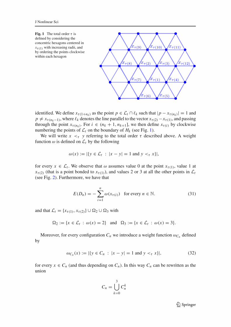
J Nonlinear Sci
Fig. 1 The total order τ isdefined by considering theconcentric hexagons centered inxτ (1) with increasing radii, andby ordering the points clockwisewithin each hexagon
xτ(1)
xτ(2) xτ(3)
xτ(4)
xτ(5)xτ(6)
xτ(7)
xτ(8)
xτ(9) xτ(10) xτ(11)
xτ(12)
identified. We define xτ (1+nk ) as the point p ∈ Lt ∩ ℓk such that |p − xτ (nk )| = 1 andp = xτ (nk−1), where ℓk denotes the line parallel to the vector xτ (2)−xτ (1), and passingthrough the point xτ (nk ). For i ∈ (nk + 1, nk+1], we then define xτ (i) by clockwisenumbering the points of Lt on the boundary of Hk (see Fig. 1).
We will write x <τ y referring to the total order τ described above. A weightfunction ω is defined on Lt by the following
ω(x) := |y ∈ Lt : |x − y| = 1 and y <τ x|,
for every x ∈ Lt . We observe that ω assumes value 0 at the point xτ (1), value 1 atxτ (2) (that is a point bonded to xτ (1)), and values 2 or 3 at all the other points in Lt(see Fig. 2). Furthermore, we have that
E(Dn) = −n∑
i=1
ω(xτ (i)) for every n ∈ N. (31)
and that Lt = xτ (1), xτ (2) ∪ 02 ∪ 03 with
02 := x ∈ Lt : ω(x) = 2 and 03 := x ∈ Lt : ω(x) = 3.
Moreover, for every configuration Cn we introduce a weight function ωCn definedby
ωCn (x) := |y ∈ Cn : |x − y| = 1 and y <τ x|, (32)
for every x ∈ Cn (and thus depending on Cn). In this way Cn can be rewritten as theunion
Cn =3⋃
k=0
Ckn
123

J Nonlinear Sci
Fig. 2 The first elements of Ltwith respect to the order τ areshown with their weightassigned by the value of thefunction ω appearing belowthem
xτ(1)
xτ(2) xτ(3)
xτ(4)
xτ(5)xτ(6)
xτ(7)
xτ(8)
xτ(9) xτ(10) xτ(11)
xτ(12)
0
1 2
2
22
3
2
2 3 2
3
where
Ckn := x ∈ Cn : ωCn (x) = k (33)
for k = 0, . . . , 3. We notice that ωCn (x) ≤ ω(x) for every x ∈ Cn and that |C0n | is the
number of connected components of Cn .In order to prove the isoperimetric inequality (13), we first express the energy, the
perimeter, the edge perimeter, and the area of a regular configuration Cn as a functionof the cardinality of the sets Ck
n .
Proposition 2.2 Let Cn be a regular configuration in Lt . Then
E(Cn) = −|C1n | − 2|C2
n | − 3|C3n |, (34)
A(Cn) = |C2n | + 2|C3
n |, (35)
P(Cn) = 2|C1n | + |C2
n |, (36)
|!(Cn)| = 6|C0n | + 4|C1
n | + 2|C2n |, (37)
for every n ∈ N.
Proof Fix n ∈ N, and let Cn be a regular configuration in Lt . In analogy to (31) thereholds
E(Cn) = −n∑
i=1
ωCn (xi ).
For i = 0, . . . , n − 1, denote by Ci the subset of Cn containing the first i points ofCn , according to the total order τ . If xτ (i) ∈ C0
n , then
A(Ci ) − A(Ci−1) = 0, P(Ci ) − P(Ci−1) = 0 and |!(Ci )| − |!(Ci−1)| = 6;(38)
123

J Nonlinear Sci
if xτ (i) ∈ C1n , then
A(Ci ) − A(Ci−1) = 0, P(Ci ) − P(Ci−1) = 2 and |!(Ci )| − |!(Ci−1)| = 4;(39)
if xτ (i) ∈ C2n , then
A(Ci ) − A(Ci−1) = 1, P(Ci ) − P(Ci−1) = 1 and |!(Ci )| − |!(Ci−1)| = 2;(40)
whereas, if xτ (i) ∈ C3n , we have
A(Ci ) − A(Ci−1) = 2, P(Ci ) − P(Ci−1) = 0 and |!(Ci )| − |!(Ci−1)| = 0.
(41)
In view of (38)–(41), we obtain (34)–(37). ⊓6
Wenotice that from (34),(35), and (36) we also recover (28), which in turn, togetherwith (37), yields
E(Cn) = −32A(Cn) − 1
4|!(Cn)| +
32|C0
n | (42)
for every configuration Cn . Moreover, from the equality
3∑
i=0
|Cin| = n,
(35), and (36) it follows that
A(Cn) = 2n − 2|C0n | − P(Cn). (43)
Note that in particular ifCn = Dn thenωCn (x) = ω(x). Furthermore,D0n = xτ (1),
D1n = xτ (2), D2
n = 02 ∩ Dn , and D3n = 03 ∩ Dn . Therefore, (34)–(42) yield
E(Dn) = −1 − 2|02 ∩ Dn| − 3|03 ∩ Dn|, (44)
A(Dn) = |02 ∩ Dn| + 2|03 ∩ Dn|, (45)
P(Dn) = 2+ |02 ∩ Dn|, (46)
|!(Dn)| = 10+ 2|02 ∩ Dn|, (47)
and by (42) and (43) we obtain
E(Dn) = −32A(Dn) − 1
4|!(Dn)| +
32,
123

J Nonlinear Sci
and
A(Dn) = 2n − 2 − P(Dn)
for every n > 1.
Proposition 2.3 The following assertions are equivalent and hold true for every con-nected configuration Cn:
(i) |!(Dn)| ≤ |!(Cn)|;(ii) P(Dn) ≤ P(Cn);(ii) A(Dn) ≥ A(Cn).
Proof The first assertion follows directly from (30) and is equivalent to the second by(36) and (37). The second assertion is equivalent to the third by (29) and (30). ⊓6
2.1 Proof of Theorem 1.1
In this subsection, we prove Theorem 1.1 by characterizing the minimizers of EIP asthe solutions of a discrete isoperimetric problem. We proceed in two steps.Step 1 We claim that
√A(Dn) = kn P(Dn). (48)
Indeed, by (11), (12), (30), (44), there holds
θn
2− 3n = en = E(Dn) = −1 − 2|02 ∩ Dn| − 3|03 ∩ Dn|. (49)
Equalities (12) and (47) yield
θn = |!(Dn)| = 10+ 2|02 ∩ Dn|. (50)
Theorefore, by (49) and (50), we have
|02 ∩ Dn| =θn
2− 5, (51)
and
|03 ∩ Dn| = −θn
2+ n + 3. (52)
Claim (48) follows now by (45), (46), (51) and (52), and by observing that
√A(Dn) =
√|02 ∩ Dn| + 2|03 ∩ Dn| =
√θn/2 − 5+ 2(−θn/2+ n + 3)
=√
−θn/2+ 2n + 1 = kn(θn/2 − 3) = kn(|02 ∩ Dn| + 2) = kn P(Dn).
123

J Nonlinear Sci
Inequality (13) is a direct consequence of (48) and Proposition 2.3. By Propo-sition 2.3 we also deduce that the maximal area and the minimal perimeter amongconnected configurations are realized by A(Dn) = −θn/2 + 2n + 1 and P(Dn) =θn/2 − 3, respectively.Step 2We prove the characterization statement of Theorem 1.1. LetCn be a connectedconfiguration satisfying
√A(Cn) = kn P(Cn). (53)
We claim that Cn is a minimizer. In fact, the claim follows from
|!(Dn)| ≤ |!(Cn)| = 6n − 3A(Cn) − P(Cn)
= 6n − 3(kn)2(P(Cn))2 − P(Cn)
≤ 6n − 3(kn)2(P(Dn))2 − P(Dn)
= 6n − 3A(Dn) − P(Dn) = |!(Dn)|
where we used (30) in the first inequality, (29) in the first and last equality, (28) in thesecond, (53) in the third, Proposition 2.3 in the second inequality, and (48) in the thirdequality.
Viceversa, let Mn be a connected minimizer. By (10), (36), and (37), P(Mn) =P(Dn); by (28), A(Mn) = A(Dn). Thus (13) holds with the equality by (48). Thisconcludes the proof of the theorem.
3 Maximal Hexagons Associated to EIP Minimizers
In this section, we introduce the notion of maximal hexagons HrMnassociated to
minimizers Mn and we provide a uniform lower estimate of rMn in terms of n [see(69)].
Fix a minimizer Mn . Let HMns be the family of the configurations contained in
Mn that can be seen as translations in Lt of daisy configurations D1+3s+3s2 for somes ∈ N ∪ 0, i.e.,
HMns := Hs ⊂ Lt : Hs := D1+3s+3s2 + q for some q ∈ Lt and Hs ⊂ Mn, (54)
and choose HrMnto be a configuration inHMn
rMnwhere
rMn := maxs ∈ N ∪ 0 : HMns = ∅. (55)
We will refer to HrMnas the maximal hexagon associated to Mn . Notice that the
number of atoms of Mn contained in HrMnis
n(rMn ) := 1+ 3 rMn + 3(rMn
)2. (56)
123
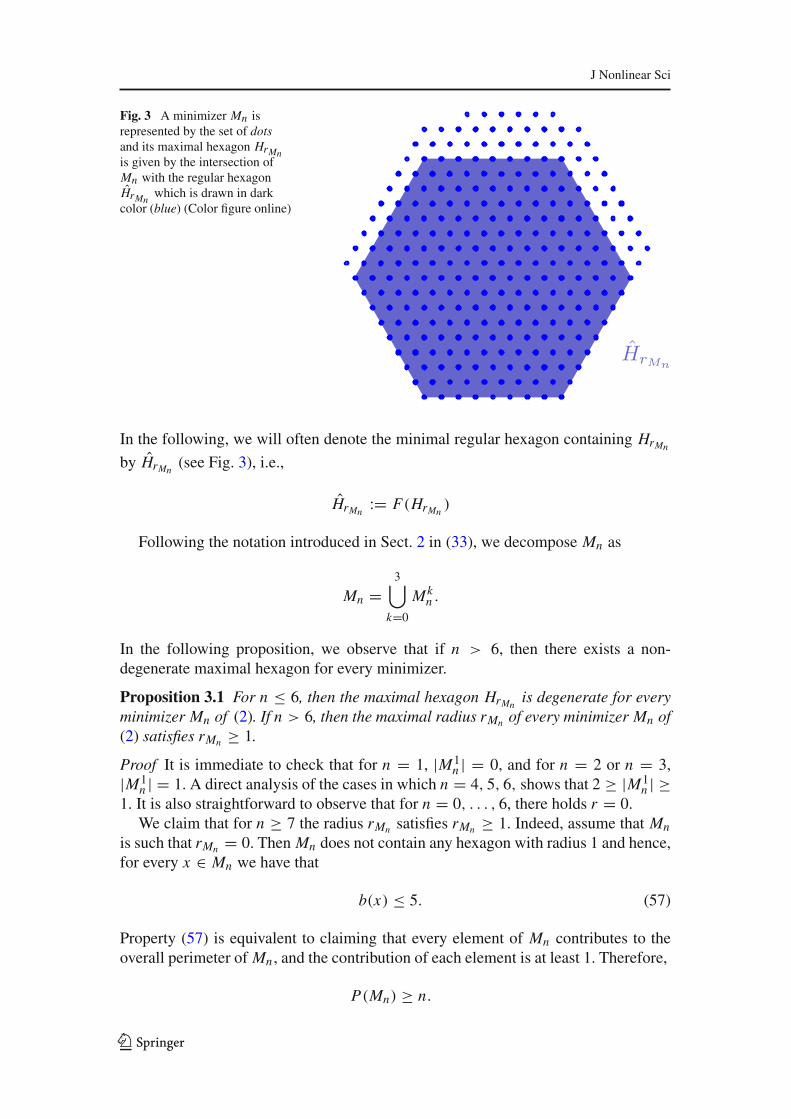
J Nonlinear Sci
Fig. 3 A minimizer Mn isrepresented by the set of dotsand its maximal hexagon HrMnis given by the intersection ofMn with the regular hexagonHrMn
which is drawn in darkcolor (blue) (Color figure online)
HrMn
In the following, we will often denote the minimal regular hexagon containing HrMn
by HrMn(see Fig. 3), i.e.,
HrMn:= F(HrMn
)
Following the notation introduced in Sect. 2 in (33), we decompose Mn as
Mn =3⋃
k=0
Mkn .
In the following proposition, we observe that if n > 6, then there exists a non-degenerate maximal hexagon for every minimizer.
Proposition 3.1 For n ≤ 6, then the maximal hexagon HrMnis degenerate for every
minimizer Mn of (2). If n > 6, then the maximal radius rMn of every minimizer Mn of(2) satisfies rMn ≥ 1.
Proof It is immediate to check that for n = 1, |M1n | = 0, and for n = 2 or n = 3,
|M1n | = 1. A direct analysis of the cases in which n = 4, 5, 6, shows that 2 ≥ |M1
n | ≥1. It is also straightforward to observe that for n = 0, . . . , 6, there holds r = 0.
We claim that for n ≥ 7 the radius rMn satisfies rMn ≥ 1. Indeed, assume that Mnis such that rMn = 0. Then Mn does not contain any hexagon with radius 1 and hence,for every x ∈ Mn we have that
b(x) ≤ 5. (57)
Property (57) is equivalent to claiming that every element of Mn contributes to theoverall perimeter of Mn , and the contribution of each element is at least 1. Therefore,
P(Mn) ≥ n.
123

J Nonlinear Sci
By Theorem 1.1, it follows that
θn
2− 3 ≥ n, (58)
which in turn by (12) implies
√12n − 3 − 2 ≥ ⌈
√12n − 3⌉ − 3 ≥ n,
that is
n2 − 8n + 7 ≤ 0,
which finally yields 1 ≤ n ≤ 7. To conclude, it is enough to notice that for n = 7,θn/2 − 3 = 6, thus contradicting (58). ⊓6
In view of Proposition 3.1 for every minimizer Mn with n > 6, we can fix a vertexV0 of its (non-degenerate) hexagon HrMn
and denote by V1, . . . , V5 the other verticesof HrMn
numbered counterclockwise starting from V0. For k = 0, . . . , 4, let us alsodenote by sk the line passing through the side of HrMn
with endpoints Vk and Vk+1,and let s5 be the line passing through V5 and V0.
In the followingwewill need to consider the number of levels of atoms inLt aroundHrMn
containing at least one element of Mn . Denote by ek the outer unit normal to theside sk of HrMn
and define
λk := max j ∈ N : s jk ∩ Mn = ∅ (59)
where s jk are the lines of the latticeLt parallel to sk and not intersecting HrMn, namely
s jk := sk +√32
jek
for j ∈ Z. Let also πk be the open half-plane with boundary sk and not intersectingthe interior of HrMn
.We first show that Mn satisfies a connectedness property with respect to the
directions determined by the lattice Lt . To this purpose, we introduce the notionof 3-convexity with respect to Lt .
Definition 3.2 We recall that
t1 := (1, 0) , t2 :=(12,
1
2√3
), and define t3 := t2 − t1.
We say that a set S ⊂ Lt is 3-convex if for every p, q ∈ S such that q := m t i + pfor some m ∈ N and i ∈ 1, 2, 3 one has that q ′ := m′ t i + p ∈ S for every integerm′ ∈ (0,m). Furthermore, we refer to the lines
123

J Nonlinear Sci
ℓpi := q ∈ R2 : q = r t i + p for some r ∈ R
as the lines of the lattice Lt at p.
Note that by Definition 3.2 a set S is 3-convex if there is no line ℓpi of the lattice Lt at
a point p ∈ Lt \ S that is separated by p in two half-lines both containing points ofthe set S.
Proposition 3.3 Let Mn be a minimizer. Then Mn is 3-convex.
Proof For the sake of contradiction assume that the minimizer Mn is a not 3-convex.Then there exist a point p ∈ Lt \ Mn and i ∈ 1, 2, 3 such that the line ℓ
pi (see
Definition 3.2) is divided by p in two half-lines both containing points of Mn . Weclaim that we can rearrange the n points of Mn in a new 3-convex configuration Mnsuch that |!(Mn)| < |!(Mn)| thus contradicting optimality.
Denote for simplicity ℓ0 := ℓpi and let ℓ1, . . . , ℓm be all the other lines parallel to ℓ0
that intersect Mn . Furthermore, let ck = |Mn ∩ℓk | for k = 1, . . . ,m. Starting from theelements of the sequence ck, we rearrange them in a decreasing order, constructinganother set dk with the property that d0 ≥ d1 ≥ · · · ≥ dm . Finally, we separate theelements of dk having odd indexes from those having even indexes and we rearrangethem in a new set fk obtained by first considering the elements of dk with evenindexes, in decreasing order with respect to their indexes, and then the elements of dkhaving odd indexes, with increasing order with respect to their indexes. The set fkconstructed as above has the property that the two central elements have the maximalvalue, and the values of the elements decrease in an alternated way by moving towardthe sides of the ordered set. Let k be the index corresponding to the central elementof the set fk, if m is even, and to the maximum between the two central elements of fk, if m is odd.
As an example, if we start with a set ck = 9, 4, 2, 5, 3, 1, 17, the sequence dkis given by 17, 9, 5, 4, 3, 2, 1 and the sequence fk by 1, 3, 5, 17, 9, 4, 2. Herek = 4.
Fix a point Pk ∈ Lt and an angular sector S of amplitude 2π/3, with vertex in Pk ,whose sides σ1 and σ2 lay on the two lines departing from Pk which are not parallelto ℓ0. Consider the points P0, . . . , Pk−1 ∈ σ1 ∩ Mn , such that
|Pk − Pk | = k − k for k = 0, . . . k − 1.
Analogously, consider the points Pk+1, . . . , Pm ∈ σ2 ∩ Mn , satisfying
|Pk − Pk | = k − k for k = k + 1, . . . ,m.
For k = 0, . . . ,m, let ℓk be the line parallel to ℓ0 and passing through Pk . To constructthe set Mn , we consider fk consecutive points on each line ℓk , starting from Pk .We notethat |Mn| = |Mn| = n, the number of bonds in each line parallel to ℓ0 has increased.On the other hand, the number of bonds between different lines has not decreased.Indeed, given two parallel lines with a and b points, respectively, the maximal number
123

J Nonlinear Sci
of bonds between these two lines is either 2a if a < b, or 2a − 1 if a = b. Thismaximal value is achieved by construction by the modified configuration. Hence,
|!(Mn)| < |!(Mn)|,
providing a contradiction to the optimality of Mn . ⊓6
Since every minimizer Mn is 3-convex, the quantity λk introduced in (59) fork = 0, . . . , 5 provides the number of non-empty levels of atoms in Mn ∩πk for n > 6.In fact, by the definition of τ each partially full level contains at least one point in(M1
n ∪ M2n ) \ HrMn
. Hence,
5∑
k=0
λk ≤ |M1n \ HrMn
| + |M2n \ HrMn
|. (60)
On the other hand,
2|M1n \ HrMn
| + |M2n \ HrMn
| = P(Mn) − P(HrMn) = pn − 6 rMn . (61)
Therefore, by (60) and (61),
5∑
k=0
λk ≤ pn − 6 rMn . (62)
In the remaining part of this section, we provide a characterization of the geometryof Mn \ HrMn
for n > 6, by subdividing this set into good polygons Pk and badpolygons Tk , and by showing that the cardinality of Mn \ HrMn
is, roughly speaking,of the same order of magnitude as the one of the union of good polygons.
Given a minimizer Mn and its maximal hexagon HrMn, we denote by HrMn+1 the
hexagon with side rMn + 1 and having the same center as HrMn. In the following, we
denote the hexagon containing HrMn+1 by
HrMn+1 := F(HrMn+1).
We first show that, by the optimality of HrMn, there exists an angular sector of 2π/3,
and centered in one of the vertices of HrMn+1, which does not intersect Mn . To thisend, we denote by V ′
i , i = 0, . . . , 5 the vertices of the hexagon HrMn+1, with theconvention that V ′
i lies on the half-line starting from the center of HrMnand passing
through Vi .
Lemma 3.4 Let Mn be a minimizer with rMn > 0. Then
(i) The hexagon HrMn+1 presents at least a vertex, say V ′j with j ∈ 0, . . . , 5, that
does not belong to Mn.
123

J Nonlinear Sci
(ii) There exists k ∈ 0, . . . , 5 such that the open angular sector Sk of amplitude2π/3, centered in V ′
k , and with sides s1k and s1k−1 (with the convention thats1−1 := s15 ) is such that Sk ∩ Mn = ∅.
(iii) Every translation H of HrMn+1 by a vector t := n t1+m t2 with n,m ∈ Z that hasa vertex v /∈ Mn admits a vertexw /∈ Mn (possibly different from v) and an openangular sector S of amplitude 2π/3 and centered in w such that S ∩ Mn = ∅.
Proof We begin by showing assertion (i). In view of the maximality of HrMnthere
exists a point p ∈ Lt on the boundary of HrMn+1 such that p /∈ Mn . Either p is alreadya vertex of HrMn+1 or p is an internal point on the side of HrMn+1 parallel to s j forsome j . In this latter case, by the 3-convexity of Mn , either V ′
j or V′j+1 does not belong
to Mn and hence, also in this case assertion (i) holds true.We now denote by V ′
j themissing vertex of the hexagon HrMn+1 and prove assertion(i i). Let us consider the two half-lines in which V ′
j divides the line s1j . By the 3-convexity of Mn , at least one of them does not intersect Mn . Analogously, if weconsider the two half-lines in which V ′
j divides the line s1j−1, by the 3-convexity of
Mn at least one of them does not intersectMn . Finally, if we consider the line s′ passingthrough the center of HrMn
and V ′j , the 3-convexity of Mn implies that the points of s′
whose distance from the center of HrMnis bigger than rMn + 1 do not belong to Mn .
In view of the geometric position of such three half-lines departing from V ′j , we can
conclude that the claim holds true by using once again the 3-convexity of Mn .Let us conclude by observing that assertion (i i i) follows by a similar argument to
the one employed to prove assertion (i i). If the center of H is in Mn , then the sameargument works and we can chose w = v. If the center of H is not in Mn , then theline passing through the missing vertex v and the center of H does not intersect Mnoutside H either for v or for the opposite vertex w with respect to the center of H . ⊓6
In the following, we assume without loss of generality that the vertex V0 has beenchosen so that the index k in assertion (i i) of Lemma 3.4 is 0. Therefore, by assertion(i i) of Lemma 3.4 we obtain that the open angular sector S0 of 2π/3, centered in V ′
0,and with sides s10 and s15 is such that S0 ∩ Mn = ∅.
Let us use the definition of the levels λk for k = 0, . . . , 5 introduced in (59) todefine a region R that contains all extra points of Mn , i.e., points of Mn not containedin HrMn
. We already know that we can take R ⊂ (R2 \ HrMn) ∩ (R2 \ S0). We define
the region R as follows (see Fig. 4):
R :=( 5⋃
j=0
Pj
)⋃( 5⋃
j=1
T j
)(63)
The set P0 in (63) is the polygon delimited by the lines s5, s10 , sλ00 , s−r+1
5 and the setsPk in (63) is defined by
Pk :=P1k (λk) if λk ≤ λk−1 + 1,
P1k (λk − λk−1 + 1) ∪ P2
k (λk − λk−1 + 1) if λk > λk−1 + 1,
123

J Nonlinear Sci
Fig. 4 Representation of theregion R given by the union ofthe polygons Pj withj = 0, . . . , 5 drawn in thelightest color (yellow) and thepolygons T j with j = 1, . . . , 5drawn in the middle color(green). Note that this picturehas a mere illustrative purpose(the configuration is not a EIPminimizer) (Color figure online)
HrMn
P1P0
P2 P5
P3 P4
T1
T2
T3
T4
T5
for every k = 1, . . . , 5, where for every a ∈ [−2 rMn , 2 rMn ] we denote by P1k (a) the
polygon contained between s1k , sak , sk+1, s−r+1
k+1 , and by P2k (a) the set delimited by sak ,
sλkk , sλk−1−r+1
k−1 , sλk−1k−1 . Finally the sets Tk are the region between Pk−1 and Pk or, more
precisely,
Tk :=x ∈ R : x ∈ s jk−1k−1 ∩ s jkk , with 1 ≤ jk−1 ≤ λk−1, 1 ≤ jk ≤ λk, jk−1 ≥ jk
and, if λk−1 > λk−2 + 1, jk−1 ≤ jk + λk−1 − λk−2. (64)
Note that T1 by definition (64) reduces to a segment contained in the line s−rMn2 such
that
|T1| = minλ0, λ1. (65)
Furthermore, we consider the configurations Pk := Pk ∩ Lt for k = 0, . . . , 5,Tk := Tk ∩ Lt for k = 1, . . . , 5, and R := R ∩ Lt . We notice that Mn ⊂ HrMn
∪ Rand that
n = |HrMn| + |R| − |R \ Mn|,
123

J Nonlinear Sci
where |HrMn| = 1+ 3 rMn + 3
(rMn
)2, and
|R| =5∑
k=0
|Pk | +5∑
k=1
|Tk | = rMn
5∑
k=0
λk +5∑
k=1
|Tk |
where in the last equality we used that |Pk | = rMnλk for k = 0, . . . , 5. Furthermore,for every x ∈ R and every k = 0, . . . , 5 there exists jk ∈ [−λk′ − 2r, λk] withk′ := (k + 3)mod 6 and k′ ∈ 0, . . . , 5 such that x ∈ s jkk . Hence, in particular, everyx ∈ R is uniquely determined by a pair of indexes ( jk, jk′), with k′ = k + 3 in Z6.
Proposition 3.5 Let H be the family of the configurations that can be seen as trans-lations in Lt of the daisy configuration D1+3s+3s2 for s := rMn + 1 and that arecontained in HrMn
∪ R, i.e.,
H := H ⊂ HrMn∪ R : H = D1+3s+3s2 + q for s := rMn + 1 and some q ∈ Lt .
Then there holds
|R \ Mn| ≥ |H|.
Proof Let h := |H|. We show by induction on m = 1, . . . , h that for every familyHm ⊂ H with |Hm | = m, there exists a set VHm ⊂ R \ Mn with |VHm | = m, suchthat the correspondence that associates to each v ∈ VHm a hexagon H ∈ Hm if v is avertex of H := F(H), is a bijection.
We remark that the thesis will follow once we prove the assertion for m = h.The claim holds for m = 1 by reasoning in the same way as in the first assertion ofLemma 3.4. Assume now that the claim is satisfied for m = m. Consider a familyHm+1 = H1, . . . , Hm+1 ⊂ H, and the polygon
Pm+1 :=m+1⋃
i=1
Hi ⊂ HrMn∪ R.
Furthermore, let us define
Pm+1 := F(Pm+1).
We subdivide the remaining part of the proof into 4 steps.
Step 1 There exists a vertex v of Pm+1 that is not in Mn . Indeed, if all vertices of Pm+1belong to Mn , by 3-convexityPm+1 ⊂ Mn , and hence Hm+1 ⊂ Pm+1 ⊂ Mn , whichwould contradict the maximality of rMn .
Step 2 By assertion (i i i) of Lemma 3.4 there exists a vertex w of Pm+1 not in Mn andan open angular sector S centered in w, amplitude 2π/3, and sides σ1, σ2 ⊂ Lt suchthat S ∩ Mn = ∅.
123

J Nonlinear Sci
Step 3 There exists a vertex v of Pm+1 that is not in Mn and that corresponds to aninterior angle of Pm+1 of 2π/3. In fact, Pm+1 can have vertices with angles of 2π/3,4π/3, and 5π/3 only. If the vertex w detected in Step 2 corresponds to an angle of2π/3, there is nothing to prove. If w corresponds to an angle of 4π/3 or 5π/3, thenwe have two cases.
Case 1 The intersection between S and the closure of Pm+1 is empty. Then, forevery j = 1, 2, there exists v j ∈ σ j such that the segment with endpoints w andv j denoted by wv j is contained in ∂Pm+1 and v j is a vertex of Pm+1. Furthermore,v j /∈ Mn because v j ∈ S, and v j is associated to an angle of 2π/3, since S∩Pm+1 = ∅.The proof follows by taking v = v1.
Case 2 The intersection between S and the closure of Pm+1 is nonempty. Withoutloss of generality, we can assume that the two sides of the angular sector S are givenby
σ1 =(α,β) ∈ R2 : β = α t1 + w, α > 0
and
σ2 =(α,β) ∈ R2 : β = −α t2 + w, α > 0
.
Define
σ k1 := σ1 −
√32
k (0, 1) and σ k2 := σ2 + k t1,
for k ∈ N. Since Pm+1 ∩ S is bounded, we can find
k1 := maxk ∈ N : σ k1 ∩ Pm+1 ∩ S = ∅
and
k2 := maxk ∈ N : σ k2 ∩ Pm+1 ∩ S = ∅.
For j = 1, 2, the intersection σk jj ∩∂Pm+1 ∩ S is a segment with at least one endpoint
v ∈ S corresponding to a vertex of ∂Pm+1 associated to an angle of 2π/3.
Step 4 Let v be the vertex provided by Step 3. Then, there exists a unique H j ∈ Hm+1
having v among its vertices. By the induction hypothesis on H1, . . . , Hm+1 \ H j there exists a family of vertices v j j=1,...,m+1, j = j ⊂ R \ Mn such that v j is a vertex
of H j and for every i = j , v j is not a vertex of Hi . The thesis follows then by settingv j = v, and by taking VHm+1 = v1, . . . , vm+1. ⊓6
In view of Proposition 3.5 in order to estimate from below the cardinality of R\Mn ,it suffices to estimate the cardinality ofH. To this end, we denote in the following by
123

J Nonlinear Sci
Uk the closure of the region in R2 containing HrMnand delimited, respectively, by s3,
s4, and s5 for k = 2, s4, s5, and s0 for k = 3, s5, s0, and s1 for k = 4, and s0, s1, ands2 for k = 5. Notice that Tk ⊂ Uk (see Fig. 5).
Lemma 3.6 There holds
|H| ≥5∑
j=2
|Tj | − λ1 − 2λ2 − 2λ3 − 2λ4 − λ5 + 4. (66)
Proof For notational simplicity we will omit in the rest of this proof the dependenceof the radius rMn on the minimizer Mn . We begin by noticing that
|H| ≥5∑
k=2
|Hk | (67)
where
Hk := H ∈ H : H ⊂ Uk and has a vertex in Tk
for k = 2, 3, 4, 5. We claim that
|Hk | ≥ |Tk | − λk − λk−1 + 1 (68)
and we observe that (66) directly follows from (67) and (68).The rest of the proof is devoted to show (68). Let x ∈ Tk and consider
( jk, jk−1, jk−2) such that x ∈ s jkk ∩ s jk−1k−1 ∩ s jk−2
k−2 . In the following, we identify xwith the triple of indexes ( jk, jk−1, jk−2), and we write x = ( jk, jk−1, jk−2). Let Hxbe the hexagon with vertices x ,
v1 := ( jk − (r + 1), jk−1, jk−2 + (r + 1)),
v2 := ( jk − 2(r + 1), jk−1 − (r + 1), jk−2 + (r + 1)),
v3 := ( jk − 2(r + 1), jk−1 − 2(r + 1), jk−2),
v4 := ( jk − (r + 1), jk−1 − 2(r + 1), jk−2 − (r + 1)),
v5 := ( jk, jk−1 − (r + 1), jk−2 − (r + 1))
(see Fig. 5 for an example of an hexagon Hx ∈ H2 with x ∈ T2).Hx is contained in Uk if for every j = 0, . . . , 5 there holds v j ∈ Uk . This latter
condition is equivalent to checking that the following inequalities are satisfied
jk − 2(r + 1) ≥ −2r, jk ≤ λk,
jk−1 − 2(r + 1) ≥ −2r, jk−1 ≤ λk−1,
jk−2 − (r + 1) ≥ −2r, jk−2 + (r + 1) ≤ λk−2.
123
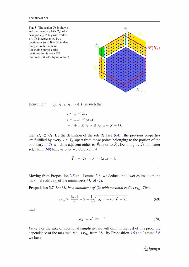
J Nonlinear Sci
Fig. 5 The region U2 is shownand the boundary ∂F(Hx ) of ahexagon Hx ∈ H2 with vertexx ∈ T2 is represented by acontinuous (red) line. Note thatthis picture has a mereillustrative purpose (theconfiguration is not a EIPminimizer) (Color figure online)
P1
HrMn
P1P0
P2
T1
T2 ∂F (Hx)
Hence, if x = ( j j , jk−1, jk−2) ∈ Tk is such that
2 ≤ jk ≤ λk,
2 ≤ jk−1 ≤ λk−1,
− r + 1 ≤ jk−2 ≤ λk−2 − (r + 1),
then Hx ⊂ Uk . By the definition of the sets Tk [see (64)], the previous propertiesare fulfilled by every x ∈ Tk , apart from those points belonging to the portion of theboundary of Tk which is adjacent either to Pk−1 or to Pk . Denoting by Tk this latterset, claim (68) follows once we observe that
|Tk | = |Tk | − λk − λk−1 + 1.
⊓6
Moving from Proposition 3.5 and Lemma 3.6, we deduce the lower estimate on themaximal radii rMn of the minimizers Mn of (2).
Proposition 3.7 Let Mn be a minimizer of (2) with maximal radius rMn . Then
rMn ≥ ⌈αn⌉6
− 2 − 16
√⌈αn⌉2 − (αn)2 + 75 (69)
with
αn :=√12n − 3 . (70)
Proof For the sake of notational simplicity, we will omit in the rest of this proof thedependence of the maximal radius rMn from Mn . By Proposition 3.5 and Lemma 3.6we have
123

J Nonlinear Sci
|R \ Mn| ≥5∑
j=2
|Tj | − λ1 − 2λ2 − 2λ3 − 2λ4 − λ5 + 4,
and so, by (62) and (65), we obtain
n = |HrMn| + |R| − |R \ Mn|
≤ 1+ 3r2 + 3r+5∑
j=0
|Pj |+5∑
j=1
|Tj |−5∑
j=2
|Tj |+λ1 + 2λ2 + 2λ3 + 2λ4 + λ5 − 4
≤ 1+ 3r2 + 3r + r5∑
j=0
λ j + |T1| + λ1 + 2λ2 + 2λ3 + 2λ4 + λ5 − 4
≤ 1+ 3r2 + 3r + (r + 2)5∑
j=0
λ j − 4
≤ 1+ 3r2 + 3r + (r + 2)(pn − 6r) − 4 = −3r2 + (pn − 9)r + 2pn .
Thus, the maximal radius satisfies the following inequality:
3r2 − (pn − 9)r + n − 2pn ≤ 0. (71)
Estimate (69) follows from (71) by solving (71) with respect to r and recalling thatpn = θn/2 − 3 by Theorem 1.1 and θn = 2⌈αn⌉ by (12). ⊓6
A direct consequence of (69) is the upper bound on the Hausdorff distance betweenthe sets Mn and HrMn
introduced in Corollary 1.3.
Proof of Corollary 1.3 Let Mn be a minimizer. We assume with no loss of generalitythat n > 6 so that by Proposition 3.1 the maximal hexagon HrMn
is not degenerate.Then
dH(Mn, HrMn) ≤ max
i=0,...,5λi .
Therefore, by (62) and (70) we obtain that
dH(Mn, HrMn) ≤ pn − 6 rMn
≤ 9+√
⌈αn⌉2 − (αn)2 + 75
=√
⌈αn⌉2 − (αn)2 + O(1)
≤√2⌈αn⌉ + O(1) ≤
√2√√
12n − 3+ 1+ O(1)
≤ 2 · 31/4n1/4 + O(1)
where we used Proposition 3.7 in the second inequality. ⊓6
123

J Nonlinear Sci
4 Convergence to the Wulff Shape
In this section, we use the lower bound (69) on the maximal radius rMn associated toeach minimizer Mn of (2) to study the convergence of minimizers to the hexagonalasymptotic shape as the number n of points tends to infinity.
To this end, we recall from the introduction that W is the regular hexagon definedas the convex hull of the vectors
± 1√
3t1, ±
1√3t2, ±
1√3t3
,
where ti are defined in Definition 3.2 for i = 1, 2, 3. Furthermore, in the following µwill denote the measure
µ := 2√3χW ,
where χW is the characteristic function of W . We recall that by ∥ · ∥ we denote thetotal variation norm and by ∥ · ∥F the flat norm defined by
∥µ∥F := sup∫
R2ϕ dµ : ϕ is Lipschitz with ∥ϕ∥W 1,∞(R2) ≤ 1
(72)
for every µ ∈ Mb(R2) (see Whitney 1957).
4.1 Proof of Theorem 1.2
In this subsection, we prove Theorem 1.2.Step 1 We start by considering
Kn := ⌈αn⌉6n3/4
√⌈αn⌉2 − (αn)2, (73)
where αn := √12n − 3, see (70). In view of the definition of HrMn
, we observe that
|Mn \ HrMn| = n − (1+ 3 (rMn )
2 + 3 rMn )
≤ n − 1 − 3(⌈αn⌉
6− 2 − 1
6
√⌈αn⌉2 − (αn)2 + 33
)2
− 3(⌈αn⌉
6− 2 − 1
6
√⌈αn⌉2 − (αn)2 + 33
)
= n − ⌈αn⌉212
+ ⌈αn⌉6
√⌈αn⌉2 − (αn)2 + o(n3/4)
= ⌈αn⌉6
√⌈αn⌉2 − (αn)2 + o(n3/4) (74)
123

J Nonlinear Sci
where we used Proposition 3.7 in the inequality. Therefore, by (73) and (74) we obtainestimate (24), i.e.,
|Mn \ HrMn| ≤ Knn3/4 + o(n3/4).
Furthermore, since
∥∥∥µMn − µHrMn
∥∥∥ =∣∣MnHrMn
∣∣
n
and HrMn⊂ Mn , by (24) we also obtain that
∥∥∥µMn − µHrMn
∥∥∥ ≤ Knn−1/4 + o(n−1/4). (75)
We now define
dn := 1+ 3 rMn + 3(rMn
)2
and consider the empirical measure µDdnassociated to the daisy Ddn . For every point
xi ∈ Ddn , we denote by Zi the Voronoi cell in Lt related to xi that is the regularhexagon centered in xi with side 1/
√3 and edges orthogonal to the three lattice
directions. Furthermore, let Zni := x/√n : x ∈ Zi . We observe that
∥∥∥xi√n
− x∥∥∥L∞(Zn
i )≤ 1√
3n, (76)
and
L2
(( dn⋃
i=1
Zni
)
4W
)
=√32
Knn−1/4. (77)
For every ϕ ∈ W 1,∞(R2), we obtain that
∣∣∣∫
R2ϕ dµDn −
∫
R2ϕ dµ
∣∣∣ =∣∣∣1n
dn∑
i=1
ϕ( xi√
n
)− 2√
3
∫
Wϕ dx
∣∣∣
= 2√3
∣∣∣dn∑
i=1
ϕ( xi√
n
)L2(Zn
i ) −∫
Wϕ dx
∣∣∣
≤ 2√3
∣∣∣dn∑
i=1
∫
Zni
(ϕ( xi√
n
)− ϕ(x)
)dx
∣∣∣+ 2√3∥ϕ∥L∞(R2)L
2
⎛
⎝
⎛
⎝dn⋃
i=1
Zni
⎞
⎠4W
⎞
⎠
≤ 2√3∥∇ϕ∥L∞(R2;R2)
dn∑
i=1
∫
Zni
∣∣∣xi√n
− x∣∣∣ dx + 2√
3∥ϕ∥L∞(R2)L
2
⎛
⎝
⎛
⎝dn⋃
i=1
Zni
⎞
⎠4W
⎞
⎠
123

J Nonlinear Sci
≤ 23√n
∥∇ϕ∥L∞(R2;R2)L2
⎛
⎝dn⋃
i=1
Zni
⎞
⎠+ 2√3∥ϕ∥L∞(R2)L
2
⎛
⎝
⎛
⎝dn⋃
i=1
Zni
⎞
⎠4W
⎞
⎠
≤ 23√n
∥∇ϕ∥L∞(R2;R2)
L2(HrMn+1)
n+ 2√
3∥ϕ∥L∞(R2)L
2
⎛
⎝
⎛
⎝dn⋃
i=1
Zni
⎞
⎠4W
⎞
⎠
≤ ∥ϕ∥W 1,∞(R2)O(n−1/2)+ ∥ϕ∥L∞(R2)Knn−1/4, (78)
where we used (76) and (77) in the third and the last inequality, respectively.By combining (75) with (78), we obtain that
µM ′n
∗ µ weakly* in Mb(R2), (79)
and
∥∥µM ′n− µ
∥∥F ≤ 2Knn−1/4 + o(n−1/4), (80)
where M ′n := Mn − qn , with qn ∈ Lt such that HrMn
= D1+3rMn+3r2Mn+ qn .
Step 2Assertions (15)–(18) directly follow from (24), (75), and (80) since by (70) and(73) a direct computation shows that
Kn = ⌈αn⌉6n3/4
√⌈αn⌉2 − (αn)2
= 231/4
√⌈√12n − 3
⌉−
√12n − 3+ o(1)
= Kt
√⌈√12n − 3
⌉−
√12n − 3+ o(1) (81)
We notice here that Theorem 1.2 implies in particular the convergence (up to transla-tions) of the empirical measures associated with the minimizers to the measure µ notonly with respect to the weak∗-converge of measures, but also with respect to the flatnorm [see (72)].
We remark that an alternative approach to the one adopted in Theorem 1.2 is thatof defining a unique n-configurational Wulff shape Wn for all the minimizer with natoms. For example, we could define
Wn := Wn ∩ Lt ,
where Wn is the hexagon with side pn/6 and center xτ (1). We remark that the O(n1/4)estimate on the Hausdorff distance and the O(n3/4)-law still hold true by replacingthe maximal hexagon HrMn
with Wn .More precisely, by Proposition 3.7 we have that
dH(Wn, HrMn) ≤ 6
∣∣∣pn6
− r∣∣∣ ≤
√⌈αn⌉2 − (αn)2 + O(1) (82)
123

J Nonlinear Sci
and that
|Wn \ HrMn| ≤
∣∣∣3( ⌊ pn
6
⌋ )2+ 3
( ⌊ pn6
⌋ )− 3
(rMn
)2 − 3 rMn
∣∣∣
= 3( ⌊ pn
6
⌋+ rMn + 1
)∣∣∣⌊ pn6
⌋− rMn
∣∣∣
≤ pn6
√⌈αn⌉2 − (αn)2 + o(n3/4)
= ⌈αn⌉6
√⌈αn⌉2 − (αn)2 + o(n3/4) (83)
for every minimizer Mn . Therefore, we obtain that
dH(M ′n,Wn) ≤ O(n1/4)
by (20) and (82), and
∣∣M ′nWn
∣∣ ≤ O(n3/4) (84)
by (24) and (84), with M ′n := Mn − qn where qn ∈ Lt are chosen in such a way that
HrMn= D1+3rMn+3r2Mn
+ qn .
Furthermore, from (84) it follows that
∥∥µM ′n− µWn
∥∥ =∣∣M ′
nWn∣∣
n≤ O(n−1/4).
4.2 Proof of Theorem 1.4
In this subsection, we prove that the estimates (15)–(17) are sharp.Step 1 In this step, we show that there exists a sequence of minimizers Mn such that,denoting by Hr Mn
their maximal hexagons,
|Mn \ Hr Mn| = Knn3/4 + o(n3/4). (85)
We will explicitly construct the minimizers Mn . To this end, we denote by Hrn theclosure of the regular hexagon in R2 with center in xτ (1) and side rn defined by
rn :=⌈⌈αn⌉
6− 1
6
√⌈αn⌉2 − (αn)2
⌉,
and we introduce Hrn := Hrn ∩ Lt . Furthermore, we define
hn := pn2
− 3rn
123
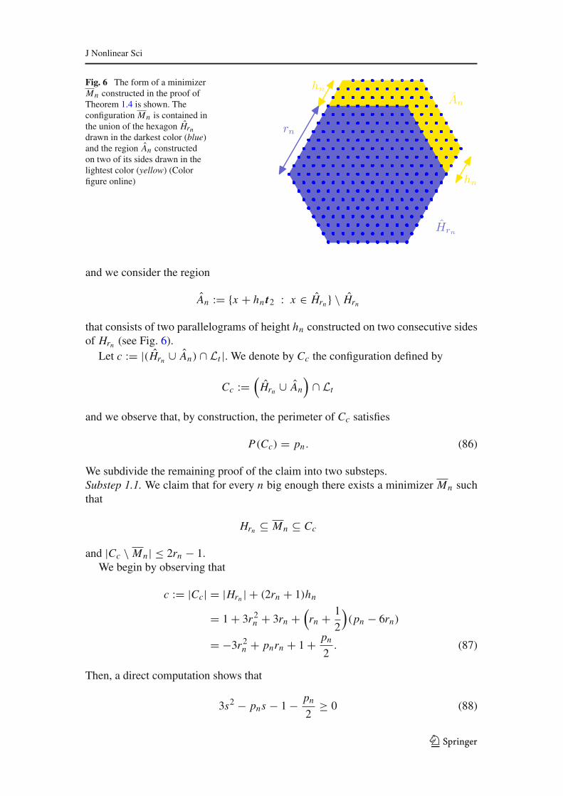
J Nonlinear Sci
Fig. 6 The form of a minimizerMn constructed in the proof ofTheorem 1.4 is shown. Theconfiguration Mn is contained inthe union of the hexagon Hrndrawn in the darkest color (blue)and the region An constructedon two of its sides drawn in thelightest color (yellow) (Colorfigure online)
An
Hrn
hn
hn
rn
and we consider the region
An := x + hn t2 : x ∈ Hrn \ Hrn
that consists of two parallelograms of height hn constructed on two consecutive sidesof Hrn (see Fig. 6).
Let c := |(Hrn ∪ An) ∩ Lt |. We denote by Cc the configuration defined by
Cc :=(Hrn ∪ An
)∩ Lt
and we observe that, by construction, the perimeter of Cc satisfies
P(Cc) = pn . (86)
We subdivide the remaining proof of the claim into two substeps.Substep 1.1. We claim that for every n big enough there exists a minimizer Mn suchthat
Hrn ⊆ Mn ⊆ Cc
and |Cc \ Mn| ≤ 2rn − 1.We begin by observing that
c := |Cc| = |Hrn | + (2rn + 1)hn
= 1+ 3r2n + 3rn +(rn +
12
)(pn − 6rn)
= −3r2n + pnrn + 1+ pn2. (87)
Then, a direct computation shows that
3s2 − pns − 1 − pn2
≥ 0 (88)
123

J Nonlinear Sci
for every s ∈[⌈αn⌉
6− 3 − 1
6
√⌈αn⌉2 + 3,
⌈αn⌉6
− 3 + 16
√⌈αn⌉2 + 3
], and, for n
big enough,
3s2 + (2 − pn)s − 2 − pn2
+ n ≥ 0 (89)
for every s ∈ R. In particular, (88) and (89) hold for s = rn and for n sufficientlylarge, yielding
0 ≤ c − n ≤ 2rn − 1. (90)
We now observe that by the definition of Cc it is possible to remove up to 2rn − 1points from Cc \ Hrn without changing the perimeter of the configuration. In view of(90), we construct Mn by removing in such a way c − n points from Cc. It followsfrom (86) that P(Mn) = pn and hence, the claim holds true.Substep 1.2. Let Mn be the sequence of ground states constructed in the previoussubstep. In view of (90), and of the definition of αn and pn , there holds
|Cn \ Hrn | = (2rn + 1)hn
= −6(rn)2 − 3rn + pnrn + 1+ pn2
= ⌈αn⌉6
√⌈αn⌉2 − (αn)2 + o(n3/4). (91)
Moreover, by the definition of Mn we have that
|Cn \ Mn| ≤ 2rn − 1 = O(n1/2) = o(n3/4). (92)
The thesis follows from combining (91) and (92) since Hrn is by construction themaximal hexagon of Mn .Step 2 In this last step, we remark that
lim supn→+∞
Kn = Kt lim supn→+∞
√⌈√12n − 3
⌉−
√12n − 3 ≤ Kt ,
and that for those n j ∈ N of the form n j = 2+ 3 j + 3 j2 there holds
Kn j → 231/4
=: Kt (93)
as j → +∞.
123

J Nonlinear Sci
In fact, we have that
√12n j − 3 =
√12(1+ 3 j + 3 j2)+ 9
= (6 j + 3)
√
1+ 12(6 j + 3)2
= 6 j + 3+ 12
(6 j + 3)[1+
√1+ 12
(6 j + 3)2
] ,
which in turn yields
⌈√12n j − 3
⌉−√12n j − 3 = 1 − 12
(6 j + 3)[1+
√1+ 12
(6 j + 3)2
] → 1
as j → +∞. ⊓6It is remarkable that the leading terms in the estimates (24), (75), and (80) estab-
lished in Step 1 of Theorem 1.2 are optimal for every n ∈ N as it follows from Step 1of the proof of Theorem 1.4.
Finally, we notice that the bounded quantities Kn defined in (73) are 0 for everyn ∈ N that can be written as n = 1+ 3k + 3k2 for some k ∈ N. This reflects the factthat for those n the daisy Dn is the unique minimizer, whose maximal hexagon HrDnis the daisy itself. Therefore, Theorem 1.4 also entails that, by adding a point to everyEIP (2) with n = 1 + 3i + 3i2 for some i ∈ N, we pass not only from a problemcharacterized by uniqueness of solutions to a problem with nonuniqueness, but alsofrom a situation of zero deviation of the minimizer from its maximal hexagon to thesituation in which minimizers include one that attains the maximal deviation.
Acknowledgements Open access funding provided by University of Vienna. The authors were supportedby the Austrian Science Fund (FWF) Project P 27052 and I 2375. This work has been funded by the ViennaScience and Technology Fund (WWTF) through project MA14-009. Partial support by the Wolfgang PauliInstitute under the thematic projectCrystals, Polymers, Materials is also acknowledged. E.D. and P.P. thankthe Center for Nonlinear Analysis (NSF Grant No. DMS-0635983), where part of this research was carriedout. E.D. was partially funded by the National Science Foundation (NSF) under Grant No. DMS- 0905778.and under the PIRE Grant No. OISE-0967140. E.D. is a member of the INDAM-GNAMPA Project 2015Critical phenomena in the mechanics of materials: a variational approach.
Open Access This article is distributed under the terms of the Creative Commons Attribution 4.0 Interna-tional License (http://creativecommons.org/licenses/by/4.0/), which permits unrestricted use, distribution,and reproduction in any medium, provided you give appropriate credit to the original author(s) and thesource, provide a link to the Creative Commons license, and indicate if changes were made.
References
Au Yeung, Y., Friesecke, G., Schmidt., B.: Minimizing atomic configurations of short range pair potentialsin two dimensions: crystallization in theWulff-shape. Calc. Var. Partial Differ. Equ. 44, 81–100 (2012)
123

J Nonlinear Sci
Bezrukov, S.L.: Edge isoperimetric problems on graphs, in: graph theory and combinatorial biology (Bal-atonlelle, 1996). Bolyai Soc. Math. Stud. 7, 157–197 (1999)
Blanc, X., Lewin, M.: The crystallization conjecture: a review. EMS Surv. Math. Sci. 2, 255–306 (2015)Cicalese, M., Leonardi, G.P.: A selection principle for the sharp quantitative isoperimetric inequality. Arch.
Ration. Mech. Anal. 206, 617–643 (2012)Davoli, E., Piovano, P., Stefanelli, U.: Wulff shape emergence in graphene. Math. Models Methods Appl.
Sci. 26(12), 2277–2310 (2016)E,W., Li, D.: On the crystallization of 2D hexagonal lattices. Commun.Math. Phys. 286, 1099–1140 (2009)Figalli, A., Maggi, F., Pratelli, A.: Amass transportation approach to quantitative isoperimetric inequalities.
Invent. Math. 182, 167–211 (2010)Flatley, L., Theil, F.: Face-centered cubic crystallization of atomistic configurations. Arch. Ration. Mech.
Anal. 218, 363–416 (2015)Fusco, N., Maggi, F., Pratelli, A.: The sharp quantitative isoperimetric inequality. Ann. of Math. (2) 168,
941–980 (2008)Harper, L.H.:Globalmethods for combinatorial isoperimetric problems. In: Cambridge Studies inAdvanced
Mathematics, vol. 90. Cambridge University Press, Cambridge (2004)Heitmann, R., Radin, C.: Ground states for sticky disks. J. Stat. Phys. 22(3), 281–287 (1980)Mainini, E., Stefanelli, U.: Crystallization in carbon nanostructures. Commun.Math. Phys. 328(2), 545–571
(2014)Mainini, E., Piovano, P., Stefanelli, U.: Finite crystallization in the square lattice. Nonlinearity 27, 717–737
(2014a)Mainini, E., Piovano, P., Stefanelli, U.: Crystalline and isoperimetric square configurations. Proc. Appl.
Math. Mech. 14, 1045–1048 (2014b)Radin, C.: The ground state for soft disks. J. Stat. Phys. 26(2), 365–373 (1981)Schmidt, B.: Ground states of the 2D sticky disc model: fine properties and N3/4 law for the deviation from
the asymptotic Wulff-shape. J. Stat. Phys. 153, 727–738 (2013)Theil, F.: A proof of crystallization in two dimensions. Commun. Math. Phys. 262, 209–236 (2006)Trillos, N.G., Slepcev, D.: Continuum limit of total variation on point clouds. Arch. Ration. Mech. Anal.
220, 193–241 (2016)Whitney, H.: Geometric Integration Theory. Princeton University Press, Princeton (1957)
123

Chapter 3
Time-evolving inelastic
phenomena
This chapter consists of the following papers:
1) E. Davoli, U. Stefanelli.
Dynamic perfect plasticity as convex minimization.
SIAM Journal on Mathematical Analysis 51 (2019), 672–730.
2) E. Davoli, T. Roubıcek, U. Stefanelli.
Dynamic perfect plasticity and damage in viscoelastic solids.
ZAMM - Zeitschrift fur Angewandte Mathematik und Mechanik (2019), to appear.


SIAM J. MATH. ANAL. c\bigcirc 2019 Society for Industrial and Applied MathematicsVol. 51, No. 2, pp. 672--730
DYNAMIC PERFECT PLASTICITY AS CONVEX MINIMIZATION\ast
ELISA DAVOLI\dagger AND ULISSE STEFANELLI\ddagger
Abstract. We present a novel variational approach to dynamic perfect plasticity. This is basedon minimizing over entire trajectories parameter-dependent convex functionals of weighted-inertia-dissipation-energy (WIDE) type. Solutions to the system of dynamic perfect plasticity are recoveredas limits of minimizing trajectories as the parameter goes to zero. The crucial compactness is achievedby means of a time discretization and a variational convergence argument.
Key words. weighted-inertia-dissipation-energy, dynamic perfect plasticity, elliptic regulariza-tion, time discretization, functions of bounded deformation
AMS subject classifications. 70H03, 70H30, 74C10, 74G65
DOI. 10.1137/17M1148864
1. Introduction. Plasticity is the macroscopic, inelastic behavior of a metalresulting from the accumulation of slip defects at its microscopic, crystalline level. Asa result of these dislocations, the behavior of the material remains purely elastic (andhence reversible) as long as the magnitude of the stress remains small, and becomesirreversible as soon as a given stress-threshold is reached. When that happens, aplastic flow is developed such that, after unloading, the material remains permanentlyplastically deformed [27].
We refer the reader to [22, 34] for an overview on plasticity models; here we focuson dynamic perfect plasticity in the form of the classical Prandtl--Reuss model [16],
\rho \"u - \nabla \cdot \sigma = 0,(1.1)
\sigma = \BbbC (Eu - p),(1.2)
\partial H( \.p) \ni \sigma D,(1.3)
describing the basics of plastic behavior in metals [20]. Here u(t) : \Omega \rightarrow \BbbR 3 denotesthe (time-dependent) displacement of a body with reference configuration \Omega \subset \BbbR 3 anddensity \rho > 0, and \sigma (t) : \Omega \rightarrow \BbbM 3\times 3
sym is its stress. In particular, relation (1.1) expressesthe conservation of momenta. The constitutive relation (1.2) relates the stress \sigma (t)to the linearized strain Eu(t) = (\nabla u(t)+\nabla u(t)\top )/2 : \Omega \rightarrow \BbbM 3\times 3
sym and the plastic
strain p(t) : \Omega \rightarrow \BbbM 3\times 3D (deviatoric tensors) via the fourth-order elasticity tensor \BbbC .
Finally, (1.3) expresses the plastic-flow rule: H : \BbbM 3\times 3D \rightarrow [0,+\infty ) is a positively
1-homogeneous, convex dissipation function, \sigma D stands for the deviatoric part of thestress, and the symbol \partial is the subdifferential in the sense of convex analysis [9]. Thesystem will be driven by imposing a nonhomogeneous boundary displacement. Detailson notation and modeling are given in section 2.
\ast Received by the editors September 22, 2017; accepted for publication (in revised form) January3, 2019; published electronically March 19, 2019.
http://www.siam.org/journals/sima/51-2/M114886.htmlFunding: The work of the author was supported by the Austrian Science Fund (FWF) projects
P 27052, I 2375, and F 65, and by the Vienna Science and Technology Fund (WWTF) projectMA14-009.
\dagger Faculty of Mathematics, University of Vienna, A-1090 Vienna, Austria ([email protected]).
\ddagger Faculty of Mathematics, University of Vienna, A-1090 Vienna, Austria, and Istituto di Matem-atica Applicata e Tecnologie Informatiche E. Magenes, I-27100 Pavia, Italy ([email protected]).
672

DYNAMIC PERFECT PLASTICITY AS CONVEX MINIMIZATION 673
The focus of this paper is on recovering weak solutions to the dynamic perfectplasticity system (1.1)--(1.3) by minimizing parameter-dependent convex functionalsover entire trajectories, and by passing to the parameter limit. In particular, weconsider the weighted-inertia-dissipation-energy (WIDE) functional of the form
(1.4) I\varepsilon (u, p) =
\int T
0
\int
\Omega
exp
\biggl( - t
\varepsilon
\biggr) \biggl( \rho \varepsilon 2
2| \"u| 2 + \varepsilon H( \.p) +
1
2(Eu - p) : \BbbC (Eu - p)
\biggr) dx dt,
to be defined on suitable admissible classes of entire trajectories t \in [0, T ] \mapsto \rightarrow (u(t), p(t)) :\Omega \rightarrow \BbbR 3 \times \BbbM 3\times 3
D fulfilling given boundary-displacement and initial conditions (on uand p, respectively). The functional bears its name from the sum of the inertialterm \rho | \"u| 2/2, the dissipative term H( \.p), and the energy term (Eu - p) : \BbbC (Eu - p)/2,weighted by different powers of \varepsilon as well as the function exp( - t/\varepsilon ).
For all \varepsilon > 0 one can prove that (a suitable relaxation of) the convex functionalI\varepsilon admits minimizers (u\varepsilon , p\varepsilon ), which indeed approximate solutions to the dynamicperfect plasticity system (1.1)--(1.3). In particular, by computing the correspondingEuler--Lagrange equations, one finds that the minimizers (u\varepsilon , p\varepsilon ) weakly solve theelliptic-in-time approximating relations,
\varepsilon 2\rho ....u\varepsilon - 2\varepsilon 2\rho
...u\varepsilon + \rho \"u\varepsilon - \nabla \cdot \sigma \varepsilon = 0,(1.5)
\sigma \varepsilon = \BbbC (Eu\varepsilon - p\varepsilon ),(1.6)
- \varepsilon (\partial H( \.p\varepsilon ))\cdot + \partial H( \.p\varepsilon ) \ni \sigma \varepsilon D,(1.7)
along with Neumann conditions at the final time T .The dynamic perfect plasticity system (1.1)--(1.3) is formally recovered by tak-
ing \varepsilon \rightarrow 0 in system (1.5)--(1.7). The main result of this paper consists of makingthis intuition rigorous, resulting in a new approximation theory for dynamic perfectplasticity.
The interest in this variational-approximation approach is threefold. First, thedifferential problem (1.1)--(1.3) is reformulated on purely variational grounds. Thisopens the possibility of applying the powerful tools of the calculus of variations to theproblem, such as the direct method, relaxation, and \Gamma -convergence [15].
Second, by addressing a time-discrete analogue of this approach we contribute anovel numerical strategy in order to approximate dynamic perfect plasticity by meansof space-time optimization and collocation methods. We believe this to be of potentialinterest in combination with global constraints or noncylindrical domains.
Eventually, the variational formulation via WIDE functionals is easily open togeneralization by including more refined material effects, especially in terms of addi-tional internal-variable descriptions. This indeed has been one of the main motivationsfor advancing the WIDE method; see, in particular, [10, 26] for applications in ma-terials science. Details of the method in the case of dynamic perfect plasticity couldthen serve as the basis for developing complete theories for evolutionary dissipativeprocesses, such as those involving damage or fracture effects.
As a by-product of our analysis, we obtain a new proof of existence of weaksolutions to dynamic perfect plasticity. Note that existence results for (1.1)--(1.3) areindeed quite classical. In the quasi-static case, in which the inertial term is neglected,they date back to Suquet [50] and have been subsequently reformulated by Dal Maso,DeSimone, and Mora [11] and Francfort and Giacomini [18] within the theory of rate-independent processes (see the recent monograph [39]). In the dynamic case boththe first existence results due to Anzellotti and Luckhaus [6, 35] and the subsequent

674 ELISA DAVOLI AND ULISSE STEFANELLI
revisiting of these results by Babadjian and Mora [7] are based on viscosity techniques.Dimension reduction has been tackled in both the quasi-static and the dynamic casein [13, 28, 29] and [36], respectively. Finally, in [12] convergence of solutions of thedynamic problem to solutions of the quasi-static problem has been shown. Withrespect to the available existence theories our approach is new, for it does not rely onviscous approximation but rather a global variational method.
Before moving on, let us review here the available literature on WIDE variationalmethods. At the level of Euler--Lagrange equations, elliptic-regularization techniquesare classical and can be traced back to Lions [32, 33] and Ole\u \inik [43]. Their variationalversion via global functionals was already mentioned in the classical textbook byEvans [17, Problem 3, p. 487] and has been used by Ilmanen [24] in the contextof Brakke mean-curvature flow of varifolds and by Hirano [23] in connection withperiodic solutions to gradient flows.
The formalism has then been applied in the context of rate-independent systemsby Mielke and Ortiz [38]; see also the follow-up paper [40]. Viscous dynamics havebeen considered in many different settings, including gradient flows [41], curves ofmaximal slopes in metric spaces [44, 45], mean-curvature flow [48], doubly nonlinearequations [1, 2, 3, 4, 5], reaction-diffusion systems [37], and quasi-linear parabolicequations [8].
The dynamic case has been the object of a long-standing conjecture by De Giorgion semilinear waves [14]. The conjecture was solved affirmatively [49] for finite-timeintervals and by Serra and Tilli [46] for the whole time semiline, that is, in its originalformulation. De Giorgi himself pointed out in [14] the interest in extending themethod to other dynamic problems. The task has then been taken up in [31] for mixedhyperbolic-parabolic equations, in [30] for Lagrangian mechanics, and in [47] for otherhyperbolic problems. The present paper delivers, in its main result (Theorem 2.3),the first realization of De Giorgi's suggestion in the context of continuum mechanics.
We briefly outline the main steps of the WIDE approach, and of the proof ofTheorem 2.3, in our setting. First, we perform a time discretization of the WIDEfunctional. By choosing suitable test functions in the discrete Euler--Lagrange equa-tions, and by performing time-discrete integration by parts, we prove in Theorem 4.8 afirst a priori estimate for minimizers of the time-discrete WIDE functionals. A crucialpoint of the argument is to guarantee that the estimate above is uniform with respectto both the WIDE parameter \varepsilon and the width of the time-discretization step. Second,we show via a \Gamma -convergence type of argument that the same uniform a priori esti-mate is fulfilled by suitable minimizers of the WIDE functional at the time-continuouslevel (see Corollary 5.3). This latter estimate guarantees compactness of sequencesof minimizers as \varepsilon tends to zero, and it allows us to recover conditions (1.1) and(1.2) in the limit. The third step (see Propositions 6.4 and 6.6) consists of deducingboth an energy inequality at the \varepsilon -level fulfilled by minimizers, and a correspondingintegrated-in-time counterpart. Finally, we pass to the limit in the energy inequalityand show that the flow rule in (1.3) is attained in weak form (see subsection 2.8).
An alternative approach to deducing a uniform energy estimate analogous to thatin Corollary 5.3 could be to try performing directly some very careful energy estimatesin the equations, along the lines of [46, 47]. We have decided here to proceed insteadas in [49], namely by first performing a discretization in time, establishing a uniforma priori estimate at the time-discrete level, and eventually showing that this estimatetransfers to the time-continuous setting.
We have chosen to adopt this latter strategy for three main reasons. First, theexistence results in the literature for solutions to both the quasi-static and the dynamic

DYNAMIC PERFECT PLASTICITY AS CONVEX MINIMIZATION 675
problem in perfect plasticity are classically proven by resorting to time discretization.Adopting the analogous strategy might allow us to gain further insight into the relationbetween classical approximations via viscosity solutions and those provided by theWIDE approach; this is currently an open question. Second, the WIDE approach forrate-independent processes has been developed by relying on a time-discrete analysis.In this regard, our analysis shows that the same methodology can be used to discussboth the quasi-static and the dynamic case. Finally, the establishment of the time-discrete a priori estimates might prove useful for advancing the study of the numericsof the problem.
The motivation for choosing dynamic perfect plasticity as a test for the WIDEmethodology is threefold. First, the existence theory in this setting has already beenfully characterized in both the quasi-static and the dynamic case. This provides a solidstarting point for our analysis that might be not available in different frameworks.Second, we are interested in checking whether the WIDE methodology is amenablealso to solving dynamic problems calling for very weak formulations in spaces of mea-sures. Third, we intend to proceed along the line proposed by De Giorgi in his seminalpaper [14, Conj. 4, Rem. 1] of extending the reach of the WIDE methodology beyondsemilinear waves. This has partly succeeded in the case of additional superlinear dissi-pation [31, 47]. Our goal is then to check whether a similar analysis applies to perfectplasticity, in which the dynamic of the system is characterized by linear dissipationinstead.
The paper is organized as follows. We introduce notation and state our mainresult, namely Theorem 2.3, in section 2. Then, we discuss in section 3 the existenceof minimizers of the WIDE functionals. In section 4 a time discretization of theminimization problem is addressed. Its time-continuous limit is discussed in section5 by means of variational convergence arguments. A parameter-dependent energyinequality is derived in section 6 and used in section 7 in order to pass to the limit as\varepsilon \rightarrow 0 and prove Theorem 2.3.
2. Statement of the main result. We devote this section to the specificationof the material model and its mathematical setting. Some notions from measuretheory need to be recalled, and we introduce the notation and assumptions to beused throughout the article. The specific form of the WIDE functionals is eventuallyintroduced in subsection 2.9, and we conclude by stating our main result, namelyTheorem 2.3.
2.1. Tensors. In what follows, for any map f : [0, T ] \times \BbbR 3 \rightarrow \BbbR we will denoteby \.f its time derivative and by \nabla f its spatial gradient. The set of 3\times 3 real matriceswill be denoted by \BbbM 3\times 3. Given M,N \in \BbbM 3\times 3, we will denote their scalar productby M : N := tr(M\top N), where tr denotes the trace and the superscript stands fortransposition, and we will adopt the notation MD to identify the deviatoric part ofM , namely MD := M - tr(M)Id/3, where Id is the identity matrix. The symbol\BbbM 3\times 3
sym will stand for the set of symmetric 3 \times 3 matrices, whereas \BbbM 3\times 3D will be the
subset of \BbbM 3\times 3sym given by symmetric matrices having null trace.
2.2. Measures. Given a Borel set B \subset \BbbR N , the symbol \scrM b(B;\BbbR m) denotesthe space of all bounded Borel measures on B with values in \BbbR m (m \in \BbbN ). Whenm = 1 we will simply write \scrM b(B). We will endow \scrM b(B;\BbbR m) with the norm\| \mu \| \scrM b(B;\BbbR m) := | \mu | (B), where | \mu | \in \scrM b(B) is the total variation of the measure \mu .
If the relative topology of B is locally compact, then by the Riesz representationtheorem the space \scrM b(B;\BbbR m) can be identified with the dual of C0(B;\BbbR m), which

676 ELISA DAVOLI AND ULISSE STEFANELLI
is the space of all continuous functions \varphi : B \rightarrow \BbbR m such that the set \ | \varphi | \geq \delta \ iscompact for every \delta > 0. The weak* topology on \scrM b(B;\BbbR m) is defined using thisduality.
2.3. Functions with bounded deformation. Let U be an open set of \BbbR 3.The space BD(U) of functions with bounded deformation is the space of all functionsu \in L1(U ;\BbbR 3) whose symmetric gradient Eu := symDu := (Du + DuT )/2 (in thesense of distributions) belongs to \scrM b(U ;\BbbM 3\times 3
sym). It is easy to see that BD(U) is aBanach space endowed with the norm
\| u\| L1(U ;\BbbR 3) + \| Eu\| \scrM b(U ;\BbbM 3\times 3sym).
A sequence \ uk\ is said to converge to u weakly* in BD(U) if uk \rightharpoonup u weakly inL1(U ;\BbbR 3) and Euk \rightharpoonup Eu weakly* in \scrM b(U ;\BbbM 3\times 3
sym). Every bounded sequence inBD(U) has a weakly* converging subsequence. If U is bounded and has a Lipschitzboundary, then BD(U) can be embedded into L3/2(U ;\BbbR 3) and every function u \in BD(U) has a trace, still denoted by u, which belongs to L1(\partial U ;\BbbR 3). If \Gamma is a nonemptyopen subset of \partial U in the relative topology of \partial U , then there exists a constant C > 0,depending on U and \Gamma such that
(2.1) \| u\| L1(U ;\BbbR 3) \leq C\| u\| L1(\Gamma ;\BbbR 3) + C\| Eu\| \scrM b(U ;\BbbM 3\times 3sym).
(See [51, Chapter II, Proposition 2.4 and Remark 2.5].) For the general properties ofthe space BD(U) we refer the reader to [51].
2.4. The elasticity tensor. Let \BbbC be the elasticity tensor, which is considereda symmetric positive-definite linear operator \BbbC : \BbbM 3\times 3
sym \rightarrow \BbbM 3\times 3sym, and let Q : \BbbM 3\times 3
sym \rightarrow [0,+\infty ) be the quadratic form associated with \BbbC , given by
Q(\xi ) :=1
2\BbbC \xi : \xi for every \xi \in \BbbM 3\times 3
sym.
Let the two constants \alpha \BbbC and \beta \BbbC , with 0 < \alpha \BbbC \leq \beta \BbbC , be such that
(2.2) \alpha \BbbC | \xi | 2 \leq Q(\xi ) \leq \beta \BbbC | \xi | 2 for every \xi \in \BbbM 3\times 3sym
and
(2.3) | \BbbC \xi | \leq 2\beta \BbbC | \xi | for every \xi \in \BbbM 3\times 3sym.
2.5. The reference configuration. Let \Omega be a bounded open set in \BbbR 3 withC2 boundary. Let \Gamma 0 be a connected open subset of \partial \Omega (in the relative topology of\partial \Omega ) such that \partial \partial \Omega \Gamma 0 is a connected, one-dimensional C2 manifold. In the followingwe will assume that \Omega is the reference configuration of our material and that \Gamma 0 is theDirichlet portion of \partial \Omega , where time-dependent boundary conditions are prescribed.
2.6. The dissipation potential. Let K be a closed convex set of \BbbM 3\times 3D such
that there exist two constants rK and RK , with 0 < rK \leq RK , satisfying
\ \xi \in \BbbM 3\times 3D : | \xi | \leq rK\ \subset K \subset \ \xi \in \BbbM 3\times 3
D : | \xi | \leq RK\ .
The boundary ofK is interpreted as the yield surface. The plastic dissipation potentialis given by the support function H : \BbbM 3\times 3
D \rightarrow [0,+\infty ) of K, defined as
H(\xi ) := sup\sigma \in K
\sigma : \xi .

DYNAMIC PERFECT PLASTICITY AS CONVEX MINIMIZATION 677
Note that K = \partial H(0) is the subdifferential of H at 0 (see, e.g., [9, section 1.4]). Thefunction H is convex and positively 1-homogeneous, with
(2.4) rK | \xi | \leq H(\xi ) \leq RK | \xi | for every \xi \in \BbbM 3\times 3D .
In particular, H satisfies the triangle inequality
(2.5) H(\xi + \zeta ) \leq H(\xi ) +H(\zeta ) for every \xi , \zeta \in \BbbM 3\times 3D .
For every \mu \in \scrM b(\Omega \cup \Gamma 0;\BbbM 3\times 3D ) let d\mu /d| \mu | be the Radon--Nikod\'ym derivative of \mu
with respect to its variation | \mu | .According to the theory of convex functions of measures [19], we introduce the
nonnegative Radon measure H(\mu ) \in \scrM b(\Omega \cup \Gamma 0), defined by
H(\mu )(A) :=
\int
A
H\Bigl( d\mu d| \mu |
\Bigr) d| \mu | ,
for every Borel set A \subset \Omega \cup \Gamma 0. We also consider the functional
\scrH : \scrM b(\Omega \cup \Gamma 0;\BbbM 3\times 3D ) \rightarrow [0,+\infty ),
defined by
\scrH (\mu ) := H(\mu )(\Omega \cup \Gamma 0) =
\int
\Omega \cup \Gamma 0
H\Bigl( d\mu d| \mu |
\Bigr) d| \mu | ,
for every \mu \in \scrM b(\Omega \cup \Gamma 0;\BbbM 3\times 3D ). Notice that \scrH is lower semicontinuous on \scrM b(\Omega \cup
\Gamma 0;\BbbM 3\times 3D ) with respect to weak* convergence. The following lemma is a consequence
of [19, Theorem 4] and [51, Chapter II, Lemma 5.2] (see also [11, subsection 2.2]).
Lemma 2.1. Setting \scrK D(\Omega ) := \ \tau \in C0(\Omega \cup \Gamma 0;\BbbM 3\times 3D ) : \tau (x) \in K for every x \in
\Omega \ , there holds
\scrH (\mu ) = sup\ \langle \tau , \mu \rangle : \tau \in \scrK D(\Omega )\ for every \mu \in \scrM b(\Omega \cup \Gamma 0;\BbbM 3\times 3
D ).
2.7. The \bfscrH -dissipation. Let s1, s2 \in [0, T ] with s1 \leq s2. For every function\mu : [0, T ] \rightarrow \scrM b(\Omega \cup \Gamma 0;\BbbM 3\times 3
D ), we define the \scrH -dissipation of t \mapsto \rightarrow \mu (t) in [s1, s2] as
D\scrH (\mu ; s1, s2)(2.6)
:= sup
\Biggl\ n\sum
j=1
\scrH (\mu (tj) - \mu (tj - 1)) : s1 = t0 \leq t1 \leq \cdot \cdot \cdot \leq tn = s2, n \in \BbbN
\Biggr\ .
Denoting by Vtot the pointwise variation of t\rightarrow \mu (t), that is,
Vtot(\mu ; s1, s2)
:= sup
\Biggl\ n\sum
j=1
\| \mu (tj) - \mu (tj - 1)\| \scrM b(\Omega \cup \Gamma 0;\BbbM 3\times 3D ) : s1 = t0 \leq \cdot \cdot \cdot \leq tn = s2, n \in \BbbN
\Biggr\ ,
by (2.4) there holds
(2.7) rKVtot(\mu ; s1, s2) \leq D\scrH (\mu ; s1, s2) \leq RKVtot(\mu ; s1, s2).

678 ELISA DAVOLI AND ULISSE STEFANELLI
As in [38, section 4.2], for every nonincreasing and positive a \in C([0, T ]) we definethe a-weighted \scrH -dissipation of t \mapsto \rightarrow \mu (t) in [s1, s2] as
D\scrH (a;\mu ; s1, s2) := sup
\Biggl\ n\sum
j=1
a(tj)\scrH (\mu (tj) - \mu (tj - 1)) : t0, tn \in [s1, s2],(2.8)
t0 \leq t1 \leq \cdot \cdot \cdot \leq tn, n \in \BbbN
\Biggr\ ,
and for every b \in C([0, T ]) we introduce the b-weighted \scrH -dissipation of t \mapsto \rightarrow \mu (t) in[s1, s2] as
(2.9) \^D\scrH (b;\mu ; s1, s2) := PMS
\int s2
s1
b(t) dD\scrH (\mu ; 0, t),
namely, as the Pollard--Moore--Stieltjes integral (see [21, sections 3 and 4]) of b withrespect to the function of bounded variation
[0, T ] \ni t \mapsto \rightarrow D\scrH (\mu ; 0, t) \in [0, D\scrH (\mu ; 0, T )].
Note that the integral above is well defined, owing to [21, Theorems 5.31 and 5.32],and that if b is nonincreasing and positive, then
(2.10) \^D\scrH (b;\mu ; s1, s2) = D\scrH (b;\mu ; s1, s2).
An adaptation of [11, Theorem 7.1] yields that if \mu is absolutely continuous in time,then
D\scrH (\mu ; s1, s2) =
\int s2
s1
\scrH ( \.\mu ) dt
and
D\scrH (a;\mu ; s1, s2) =
\int s2
s1
a(t)\scrH ( \.\mu ) dt
for every nonincreasing and positive a \in C([0, T ]).
2.8. The equations of dynamic perfect plasticity. On \Gamma 0 for every t \in [0, T ] we prescribe a boundary datum w(t) \in W 1/2,2(\Gamma 0;\BbbR 3). With a slight abuse ofnotation we also denote by w(t) a W 1,2(\Omega ;\BbbR 3)-extension of the boundary conditionto the set \Omega .
The set of admissible displacements and strains for the boundary datum w(t) isgiven by
A (w(t)) :=\Bigl\ (u, e, p) \in BD(\Omega )\times L2(\Omega ;\BbbM 3\times 3
sym)\times \scrM b(\Omega \cup \Gamma 0;\BbbM 3\times 3D ) :(2.11)
Eu = e+ p in \Omega , p = (w(t) - u)\odot \nu \scrH 2 on \Gamma 0
\Bigr\ ,
where \odot stands for the symmetrized tensor product, namely,
a\odot b := (a\otimes b+ b\otimes a)/2 \forall a, b \in \BbbR 3,
\nu is the outer unit normal to \partial \Omega , and \scrH 2 is the two-dimensional Hausdorff measure.The function u represents the displacement of the body, while e and p are called the

DYNAMIC PERFECT PLASTICITY AS CONVEX MINIMIZATION 679
elastic and plastic strain, respectively. Note that the two equalities in (2.11) hold inthe sense of \scrM b(\Omega \cup \Gamma 0;\BbbM 3\times 3
D ).We point out that the constraint
(2.12) p = (w(t) - u)\odot \nu \scrH 2 on \Gamma 0
is a relaxed formulation of the boundary condition u = w(t) on \Gamma 0 (see also [42]). Asremarked in [11], the mechanical meaning of (2.12) is that whenever the boundarydatum is not attained a plastic slip develops, whose amount is directly proportionalto the difference between the displacement u and the boundary condition w(t).
Let w \in W 2,2(0, T ;W 1,2(\Omega ;\BbbR 3)) \cap C3([0, T ];L2(\Omega ;\BbbR 3)). A solution to the equa-tions of dynamic perfect plasticity is a function t \mapsto \rightarrow (u(t), e(t), p(t)) from [0, T ] into(L2(\Omega ;\BbbR 3)\cap BD(\Omega ))\times L2(\Omega ;\BbbM 3\times 3
sym)\times \scrM b(\Omega \cup \Gamma 0;\BbbM 3\times 3D ) with u \in W 2,\infty (0, T ;L2(\Omega ;\BbbR 3))
\cap Lip(0, T ;BD(\Omega )), e \in W 1,\infty (0, T ;L2(\Omega ;\BbbR 3)), p \in Lip(0, T ;\scrM b(\Omega \cup \Gamma 0;\BbbM 3\times 3D )) such
that for every t \in [0, T ] there holds (u(t), e(t), p(t)) \in A (w(t)), and for almost everyt \in [0, T ] the following conditions are satisfied:
(c1) equation of motion: \rho \"u(t) - div \sigma (t) = 0 in \Omega and \sigma (t)\nu = 0 on \partial \Omega \setminus \Gamma 0 inthe sense of Remark 4.4, where \sigma (t) := \BbbC e(t) is the stress tensor, and \rho > 0is the constant density;
(c2) stress constraint: \sigma D(t) \in K;
(c3) energy inequality:
\int
\Omega
Q(e(t)) dx+\rho
2
\int
\Omega
| \.u(t)| 2 dx+
\int t
0
\scrH ( \.p(t)) dt \leq \int
\Omega
Q(e(0)) dx
+\rho
2
\int
\Omega
| \.u(0)| 2 dx+
\int t
0
\int
\Omega
\sigma (s) : E \.w(s) + \rho \"u(s) \cdot \.w(s) dx ds.
We remark that condition (c3) guarantees that the sum of the elastic and kineticenergies with the plastic dissipation at each time t is always less than or equal tothe sum of the initial energy with the work due to the time-dependent boundarycondition.
Under suitable assumptions, when (c1) and (c2) are satisfied, condition (c3) isindeed an equality, and it is equivalent to the following flow rule:
(c3\prime ) \.p(t) = 0 if \sigma D(t) \in intK, while \.p(t) belongs to the normal cone to K at \sigma D(t)if \sigma D(t) \in \partial K.
A detailed analysis of the equivalence between (c1)--(c3) and (c1)--(c2), (c3\prime ) hasbeen performed in [11, section 6]. An adaptation of the argument yields the analogousstatements in the dynamic setting.
The following existence and uniqueness result holds true (see [36, Theorem 3.1and Remark 3.2]).
Theorem 2.2 (existence of the evolution). Let \Omega be a bounded open set in \BbbR 3
with C2 boundary. Let \Gamma 0 be a connected open subset of \partial \Omega (in the relative topologyof \partial \Omega ) such that \partial \partial \Omega \Gamma 0 is a connected, one-dimensional C2 manifold.
Let w \in W 2,2(0, T ;W 1,2(\Omega ;\BbbR 3))\cap C3([0, T ];L2(\Omega ;\BbbR 3)) and (u0, e0, p0) \in A (w(0))be such that div\BbbC e0 = 0 a.e. in \Omega , (\BbbC e0)\nu = 0 \scrH 2-a.e. on \partial \Omega \setminus \Gamma 0, and (\BbbC e0)D \in Ka.e. in \Omega . Eventually, let (u1, e1, 0) \in A ( \.w(0)).
Then there exist unique u \in W 2,\infty (0, T ;L2(\Omega ;\BbbR 3)) \cap Lip(0, T ;BD(\Omega )),e \in W 1,\infty (0, T ;L2(\Omega ;\BbbR 3)), and p \in Lip(0, T ;\scrM b(\Omega \cup \Gamma 0;\BbbM 3\times 3
D )) solving (c1), (c2),and (c3), with (u(0), e(0), p(0)) = (u0, e0, p0), and \.u(0) = u1.

680 ELISA DAVOLI AND ULISSE STEFANELLI
2.9. The WIDE functional. Let the boundary datum
w \in W 2,2(0, T ;W 1,2(\Omega ;\BbbR 3)) \cap C3([0, T ];L2(\Omega ;\BbbR 3))
be given. By reformulating the expression in (1.4) for the triple (u, e, p) one would betempted to introduce the functional
(u, e, p) \mapsto \rightarrow \int T
0
exp\Bigl( - t
\varepsilon
\Bigr) \Bigl( \varepsilon 2\rho 2
\int
\Omega
| \"u| 2 dx+ \varepsilon \scrH ( \.p) +
\int
\Omega
Q(e) dx\Bigr) dt,
to be defined on the set \scrV , given by the class of triples (u, e, p) such that the followingconditions are fulfilled:
\scrV 1. u \in (W 2,2(0, T ;L2(\Omega ;\BbbR 3)) \cap L1(0, T ;BD(\Omega ))) with u(0) = u0, \.u(0) = u1;\scrV 2. p \in BV ([0, T ];\scrM b(\Omega \cup \Gamma 0;\BbbM 3\times 3
D )) and attains the initial datum p(0) = p0;\scrV 3. e(t) := Eu(t) - p(t) in \scrD \prime (\Omega ;\BbbM 3\times 3
sym) for every t \in [0, T ], e \in L2((0, T ) \times \Omega ;\BbbM 3\times 3
sym) and e(0) = e0;\scrV 4. (u(t), e(t), p(t)) \in A (w(t)) for a.e. t \in [0, T ],
where (u0, e0, p0) \in A (w(0)), and u1 \in W 1,2(\Omega ;\BbbR 3) is such that u1 = \.w(0) on \Gamma 0.We observe that if (u, e, p) \in \scrV , then Eu \in W 2,2(0, T ;W - 1,2(\Omega ;\BbbM 3\times 3
sym)). Thus,
e(t) is defined for every t \in [0, T ] as a map in W - 1,2(\Omega ;\BbbM 3\times 3sym) +\scrM b(\Omega \cup \Gamma 0;\BbbM 3\times 3
D ),and the initial condition e(0) = e0 is well justified. We stress that BV ([0, T ];\scrM b(\Omega \cup \Gamma 0;\BbbM 3\times 3
D )) denotes here the set of maps \mu such that \mu (t) \in \scrM b(\Omega \cup \Gamma 0;\BbbM 3\times 3D ) for
every t \in [0, T ], \mu \in L1(0, T ;\scrM b(\Omega \cup \Gamma 0;\BbbM 3\times 3D )), and Vtot(\mu ; 0, T ) < +\infty (see also
[11, Appendix]).On the other hand, one readily sees that the term
\int T
0
exp\Bigl( - t
\varepsilon
\Bigr) \scrH ( \.p) dt
is not well defined in case p is not absolutely continuous with respect to time (see [11,Theorem 7.1]). We hence need to relax the form of the WIDE functional as
I\varepsilon (u, e, p)
(2.13)
:=
\int T
0
exp\Bigl( - t
\varepsilon
\Bigr) \Bigl( \varepsilon 2\rho 2
\int
\Omega
| \"u| 2 dx+
\int
\Omega
Q(e) dx\Bigr) dt+ \varepsilon D\scrH (exp( - \cdot /\varepsilon ); p; 0, T )
for every (u, e, p) \in \scrV . As pointed out in subsection 2.7, an adaptation of [11, Theorem7.1] yields
D\scrH (exp( - \cdot /\varepsilon ); p; 0, T ) =\int T
0
exp\Bigl( - t
\varepsilon
\Bigr) \scrH ( \.p) dt
whenever p is absolutely continuous with respect to time.
2.10. Main result. We are now ready to state the main result of the paper.
Theorem 2.3 (dynamic perfect plasticity as convex minimization). Let \Omega be abounded open set in \BbbR 3 with C2 boundary. Let \Gamma 0 be a connected open subset of \partial \Omega (inthe relative topology of \partial \Omega ) such that \partial \partial \Omega \Gamma 0 is a connected, one-dimensional C2 man-ifold. Let w \in W 2,2(0, T ;W 1,2(\Omega ;\BbbR 3)) \cap C3([0, T ];L2(\Omega ;\BbbR 3)), and let (u0, e0, p0) \in A (w(0)) be such that div\BbbC e0 = 0 a.e. in \Omega , (\BbbC e0)\nu = 0 \scrH 2-a.e. on \partial \Omega \setminus \Gamma 0, and(\BbbC e0)D \in K a.e. in \Omega . Eventually, let (u1, e1, 0) \in A ( \.w(0)).

DYNAMIC PERFECT PLASTICITY AS CONVEX MINIMIZATION 681
For every \varepsilon > 0 there exists \ (u\varepsilon , e\varepsilon , p\varepsilon )\ \subset \scrV solving
(2.14) I\varepsilon (u\varepsilon , e\varepsilon , p\varepsilon ) = min
(u,e,p)\in \scrV I\varepsilon (u, e, p),
such that for \varepsilon \rightarrow 0 there holds
u\varepsilon \rightharpoonup u weakly in W 1,2(0, T ;L2(\Omega ;\BbbR 3)),
e\varepsilon \rightharpoonup e weakly in L2(0, T ;L2(\Omega ;\BbbM 3\times 3sym)).
Additionally, for every t \in [0, T ] we have
p\varepsilon (t)\rightharpoonup \ast p(t) weakly* in \scrM b(\Omega \cup \Gamma 0;\BbbM 3\times 3D ),
and for a.e. t \in [0, T ] there exists a t-dependent subsequence \ \varepsilon t\ such that
u\varepsilon t(t)\rightharpoonup \ast u(t) weakly* in BD(\Omega ),
e\varepsilon t(t)\rightharpoonup e(t) weakly in L2(\Omega ;\BbbM 3\times 3sym),
where u \in W 2,\infty (0, T ;L2(\Omega ;\BbbR 3)) \cap W 1,\infty (0, T ;BD(\Omega )), e \in W 1,\infty (0, T ;L2(\Omega ;\BbbR 3)),and p \in W 1,\infty (0, T ;\scrM b(\Omega \cup \Gamma 0;\BbbM 3\times 3
D )) is the unique solution to the dynamic perfectplasticity problem (c1), (c2), and (c3), with (u(0), e(0), p(0)) = (u0, e0, p0) and \.u(0) =u1.
The rest of the paper is devoted to the proof of Theorem 2.3. Our argument runsas follows: in section 3 we prove that minimizers \ (u\varepsilon , e\varepsilon , p\varepsilon )\ of problem (2.14) exist.Then we devise an \varepsilon -independent a priori estimate on \ (u\varepsilon , e\varepsilon , p\varepsilon )\ first in a discreteand then in a continuous setting (section 4) by means of a \Gamma -convergence argument(section 5). Finally, we derive an energy inequality at level \varepsilon > 0 (section 6) whichallows for discussing the limit \varepsilon \rightarrow 0 in section 7 and for recovering condition (c3) inthe limit.
We point out that the C2 regularity of \partial \Omega is needed in Theorem 2.3 in orderto introduce a duality between stresses and plastic strains, along the lines of [25,Proposition 2.5]. For technical reasons it is not possible to use here the results in [18]and to consider the case of a Lipschitz \partial \Omega . We refer the reader to Remark 4.6 forsome discussion of this point.
3. Minimizers of the WIDE functional. We start by focusing here on prob-lem (2.14) and show that the functional I\varepsilon admits a minimizer in \scrV .
Proposition 3.1 (existence of minimizers). For every \varepsilon > 0 there exists a triple(u\varepsilon , e\varepsilon , p\varepsilon ) \in \scrV such that
(3.1) I\varepsilon (u\varepsilon , e\varepsilon , p\varepsilon ) = inf
(u,e,p)\in \scrV I\varepsilon (u, e, p).
Proof. Fix \varepsilon > 0, and let \ (un, en, pn)\ \subset \scrV be a minimizing sequence for I\varepsilon . Wefirst observe that the triple
t\rightarrow (u0 + tu1 + w(t) - w(0) - t \.w(0), e0 + te1 + Ew(t) - Ew(0) - tE \.w(0), p0)
belongs to \scrV . Hence,
limn\rightarrow +\infty
I\varepsilon (un, en, pn) \leq \int T
0
exp\Bigl( - t
\varepsilon
\Bigr)
\cdot \Bigl( \varepsilon 2\rho
2
\int
\Omega
| \"w| 2 dx+
\int
\Omega
Q(e0 + te1 + Ew(t) - Ew(0) - tE \.w(0)) dx\Bigr) dt \leq C,

682 ELISA DAVOLI AND ULISSE STEFANELLI
thus yielding the uniform bound
supn\in \BbbN
\Bigl\ \| \"un\| L2(0,T ;L2(\Omega ;\BbbR 3)) +D\scrH (exp( - \cdot /\varepsilon ); pn; 0, T )(3.2)
+ \| en\| L2(0,T ;L2(\Omega ;\BbbM 3\times 3sym))
\Bigr\ \leq C.
Since (un, en, pn) \in \scrV , there holds pn(0) = p0 for every n \in \BbbN . In view of (2.7) and(2.8),
rK exp( - T/\varepsilon )Vtot(pn; 0, T ) \leq exp( - T/\varepsilon )D\scrH (pn; 0, T ) \leq D\scrH (exp( - \cdot /\varepsilon ); pn; 0, T ).
Therefore, we are in a position to apply the variant of Helly's theorem in [11, Lemma7.2] and to deduce the existence of a subsequence, still denoted by \ pn\ , and a mapp\varepsilon \in BV (0, T ;\scrM b(\Omega \cup \Gamma 0;\BbbM 3\times 3
D )) such that
(3.3) pn(t)\rightharpoonup \ast p\varepsilon (t) weakly* in \scrM b(\Omega \cup \Gamma 0;\BbbM 3\times 3
D ) for every t \in [0, T ],
and we have the lower semicontinuity of the \scrH -dissipation,
(3.4) D\scrH (exp( - \cdot /\varepsilon ); p\varepsilon ; 0, T ) \leq lim infn\rightarrow +\infty
D\scrH (exp( - \cdot /\varepsilon ); pn; 0, T ).
By (3.2), there exist e\varepsilon \in L2(0, T ;L2(\Omega ;\BbbM 3\times 3sym)) and u\varepsilon \in W 2,2(0, T ;L2(\Omega ;\BbbR 3)) such
that, up to the extraction of a (non--relabeled) subsequence,
(3.5) en \rightharpoonup e\varepsilon weakly in L2(0, T ;L2(\Omega ;\BbbM 3\times 3sym))
and
(3.6) un \rightharpoonup u\varepsilon weakly in W 2,2(0, T ;L2(\Omega ;\BbbR 3)).
This implies that u\varepsilon (0) = u0 and \.u\varepsilon (0) = u1. By (3.3), (3.5), and (3.6) it follows that
(3.7) en(t)\rightharpoonup e\varepsilon (t) weakly in \scrD \prime (\Omega ;\BbbM 3\times 3sym)
for every t \in [0, T ], and hence e\varepsilon (0) = e0. In view of (3.5) and Fatou's lemma, thereholds \int T
0
lim infn\rightarrow +\infty
\int
\Omega
| en| 2 dx dt \leq lim infn\rightarrow +\infty
\int T
0
\int
\Omega
| en| 2 dx dt \leq C.
Thus, by (3.7) for a.e. t \in [0, T ] there exists a t-dependent subsequence \ nt\ such that
(3.8) ent(t)\rightharpoonup e\varepsilon (t) weakly in L2(\Omega ;\BbbM 3\times 3sym).
Finally, by (2.1), (3.3), and (3.7), up to subsequences there holds
unt(t)\rightharpoonup \ast u\varepsilon (t) weakly* in BD(\Omega ) for a.e. t \in [0, T ].
The fact that p\varepsilon satisfies the Dirichlet condition on \Gamma 0 for a.e. t \in [0, T ] follows,arguing as in [11, Lemma 2.1]. The minimality of the limit triple (u\varepsilon , e\varepsilon , p\varepsilon ) is adirect consequence of the lower semicontinuity of I\varepsilon with respect to the convergencesin (3.4), (3.5), and (3.6).
We conclude this section with a result stating the uniqueness of the displacementfor a given plastic strain.

DYNAMIC PERFECT PLASTICITY AS CONVEX MINIMIZATION 683
Proposition 3.2 (uniqueness of minimizers given the plastic strain). Let(ua, ea, pa) and (ub, eb, pb) be two minimizers of I\varepsilon in \scrV . Then there exists a con-stant C such that
\varepsilon 2\| ua - ub\| 2W 2,2(0,T ;L2(\Omega ;\BbbR 3)) + \| ea - eb\| 2L2(0,T ;L2(\Omega ;\BbbM 3\times 3sym))
(3.9)
\leq C\varepsilon exp\Bigl( T\varepsilon
\Bigr) Vtot(pa - pb; 0, T ).
Proof. Arguing as in [11, Theorem 3.8], we set v = ua - ub, f = ea - eb, andq = pa - pb. Since (v(t), f(t), q(t)) \in A (0) for almost every t \in [0, T ], it follows that(ua, ea, pa) + \lambda (v, f, q) \in \scrV for every \lambda \in \BbbR . Thus,
I\varepsilon (ua, ea, pa) \leq I\varepsilon ((ua, ea, pa) + \lambda (v, f, q))
=
\int T
0
exp\Bigl( - t
\varepsilon
\Bigr) \Bigl( \varepsilon 2\rho 2
\int
\Omega
| \"ua + \lambda \"v| 2 dx+
\int
\Omega
Q(ea + \lambda f) dx\Bigr) dt
+ \varepsilon D\scrH (exp( - \cdot /\varepsilon ); pa + \lambda q; 0, T ).
By the arbitrariness of \lambda we deduce the inequality
- \varepsilon D\scrH (exp( - \cdot /\varepsilon ); q; 0, T ) \leq \int T
0
exp\Bigl( - t
\varepsilon
\Bigr) \int
\Omega
\bigl( \varepsilon 2\rho \"ua\"v + \BbbC ea : f
\bigr) dx dt(3.10)
\leq \varepsilon D\scrH (exp( - \cdot /\varepsilon ); - q; 0, T ).Arguing analogously, the minimality of (ub, eb, pb) yields
- \varepsilon D\scrH (exp( - \cdot /\varepsilon ); - q; 0, T ) \leq - \int T
0
exp\Bigl( - t
\varepsilon
\Bigr) \int
\Omega
\bigl( \varepsilon 2\rho \"ub\"v + \BbbC eb : f
\bigr) dx dt(3.11)
\leq \varepsilon D\scrH (exp( - \cdot /\varepsilon ); q; 0, T ).Summing (3.10) and (3.11) we obtain
- \varepsilon D\scrH (exp( - \cdot /\varepsilon ); pa - pb; 0, T ) - \varepsilon D\scrH (exp( - \cdot /\varepsilon ); pb - pa; 0, T )
\leq \int T
0
exp\Bigl( - t
\varepsilon
\Bigr) \int
\Omega
\bigl( \varepsilon 2\rho | \"ua - \"ub| 2 + 2Q(ea - eb)
\bigr) dx dt
\leq \varepsilon D\scrH (exp( - \cdot /\varepsilon ); pa - pb; 0, T ) + \varepsilon D\scrH (exp( - \cdot /\varepsilon ); pb - pa; 0, T ).
The thesis follows now by (2.2), (2.7), and (2.8).
We point out that minimizers of I\varepsilon are, in general, nonunique. The proof of theapproximation result in Theorem 2.3 will in fact rely on a selection of minimizers ofI\varepsilon performed via a \Gamma -convergence type of argument (see Corollary 5.3).
4. Discrete energy estimate. With the aim of establishing an a priori estimateon \ (u\varepsilon , e\varepsilon , p\varepsilon )\ independent of \varepsilon we start by analyzing a time-discrete version of theproblem. Fix n \in \BbbN , set \tau := T/n, and consider the time partition
0 = t0 < t1 < \cdot \cdot \cdot < tn = T, ti := i\tau .
We define w0 := w(0), w1 := w0 + \tau \.w(0), and, for i = 2, . . . , n, we set wi := w(ti).Our analysis will be set in the space
U\tau :=\Bigl\ (u0, e0, p0), . . . , (un, en, pn)(4.1)
\in \bigl( (BD(\Omega ) \cap L2(\Omega ;\BbbR 3))\times L2(\Omega ;\BbbM 3\times 3
sym)\times \scrM b(\Omega \cup \Gamma 0;\BbbM 3\times 3D )
\bigr) n+1:
(ui, ei, pi) \in A (wi) for i = 1, . . . , n\Bigr\ .

684 ELISA DAVOLI AND ULISSE STEFANELLI
We define the discrete energy functional I\varepsilon \tau : U\tau \rightarrow [0,+\infty ) as
I\varepsilon \tau \bigl( (u0, e0, p0), . . . , (un, en, pn)
\bigr) (4.2)
:=\varepsilon 2\rho
2
n\sum
i=2
\tau \eta \tau ,i
\int
\Omega
| \delta 2ui| 2 dx+n - 2\sum
i=2
\tau \eta \tau ,i+2
\int
\Omega
Q(ei) dx
+ \varepsilon \tau n - 1\sum
i=1
\eta \tau ,i+1\scrH (\delta pi),
where, given a vector v = (v1, . . . , vn), the operator \delta denotes its discrete derivative,
\delta vi :=vi - vi - 1
\tau , \delta kvi :=
\delta k - 1vi - \delta k - 1vi - 1
\tau ,
for k \in \BbbN , k > 1, and where the Pareto weights
(4.3) \eta \tau ,i :=
\biggl( \varepsilon
\varepsilon + \tau
\biggr) i, i = 0, . . . , n,
are a discretization of the map t\rightarrow exp\bigl( - t/\varepsilon
\bigr) . Define the set
K\tau (u0, e0, p0, u1) := \ (u0, e0, p0), . . . , (un, en, pn) \in U\tau :(4.4)
u0 = u0, e0 = e0, p0 = p0, \delta u1 = u1\ .
Arguing as in Proposition 3.1 we obtain the following result.
Lemma 4.1. There exists an (n+1)-tuple of triples (u\varepsilon k, e\varepsilon k, p
\varepsilon k) such that
\bigl( (u\varepsilon 0, e
\varepsilon 0, p
\varepsilon 0),
. . . , (u\varepsilon n, e\varepsilon n, p
\varepsilon n)\bigr) \in K\tau (u
0, e0, p0, u1) and
I\varepsilon \tau \bigl( (u\varepsilon 0, e
\varepsilon 0, p
\varepsilon 0), . . . , (u
\varepsilon n, e
\varepsilon n, p
\varepsilon n)\bigr)
(4.5)
= min\bigl( (u0,e0,p0),...,(un,en,pn)
\bigr) \in K\tau (u0,e0,p0,u1)
I\varepsilon \tau \bigl( (u0, e0, p0), . . . , (un, en, pn)
\bigr) .
4.1. Discrete Euler--Lagrange equations. We first compute the discrete Euler--Lagrange equations satisfied by a minimizing (n+1)-tuple (u\varepsilon 0, e
\varepsilon 0, p
\varepsilon 0), . . . , (u
\varepsilon n, e
\varepsilon n, p
\varepsilon n).
Proposition 4.2 (discrete Euler--Lagrange equations). Let (u\varepsilon 0, e\varepsilon 0, p
\varepsilon 0), . . . ,
(u\varepsilon n, e\varepsilon n, p
\varepsilon n) be a solution to (4.5). Then
(4.6)
n\sum
i=2
\varepsilon 2\rho \eta \tau ,i
\int
\Omega
\delta 2u\varepsilon i \cdot \delta 2\varphi i dx+
n - 2\sum
i=2
\eta \tau ,i+2
\int
\Omega
\BbbC e\varepsilon i : E\varphi i dx = 0
for every \varphi i \in W 1,2(\Omega ;\BbbR 3) such that \varphi i = 0 \scrH 2-a.e. on \Gamma 0, i = 2, . . . , n. In addition,
(4.7) - \Bigl( \varepsilon
\varepsilon + \tau
\Bigr) \scrH (\xi ) - \scrH ( - \xi ) \leq
\Bigl( \tau
\varepsilon + \tau
\Bigr) \int
\Omega
\BbbC e\varepsilon i : \xi dx \leq \scrH (\xi ) +\Bigl( \varepsilon
\varepsilon + \tau
\Bigr) \scrH ( - \xi )
for every \xi \in L2(\Omega ;\BbbM 3\times 3D ), i = 2, . . . , n - 2.
Proof. Let
(v0, f0, q0), . . . , (vn, fn, qn) \in \bigl( BD(\Omega )\times L2(\Omega ;\BbbM 3\times 3
sym)\times \scrM b(\Omega \cup \Gamma 0;\BbbM 3\times 3D )
\bigr) n+1

DYNAMIC PERFECT PLASTICITY AS CONVEX MINIMIZATION 685
be such that (vi, fi, qi) \in A (0) for i = 1, . . . , n, with v0 = \delta v1 = 0, and f0 = q0 = 0.Consider the (n+1)-tuple
(u\varepsilon 0 \pm \lambda v0, e\varepsilon 0 \pm \lambda f0, p
\varepsilon 0 \pm \lambda q0), . . . , (u
\varepsilon n \pm \lambda vn, e
\varepsilon n \pm \lambda fn, p
\varepsilon n \pm \lambda qn),
with \lambda > 0. By the minimality of (u\varepsilon 0, e\varepsilon 0, p
\varepsilon 0), . . . , (u
\varepsilon n, e
\varepsilon n, p
\varepsilon n), there holds
1
\lambda I\varepsilon \tau \bigl( (u\varepsilon 0 \pm \lambda v0, e
\varepsilon 0 \pm \lambda f0, p
\varepsilon 0 \pm \lambda q0), . . . , (u
\varepsilon n \pm \lambda vn, e
\varepsilon n \pm \lambda fn, p
\varepsilon n \pm \lambda qn)
\bigr)
- 1
\lambda I\varepsilon \tau \bigl( (u\varepsilon 0, e
\varepsilon 0, p
\varepsilon 0), . . . , (u
\varepsilon n, e
\varepsilon n, p
\varepsilon n)\bigr) \geq 0.
Therefore, by (2.5) and (4.2) we deduce the inequality
- \varepsilon \tau n - 1\sum
i=1
\eta \tau ,i+1\scrH (\delta qi)(4.8)
\leq \varepsilon 2\rho
n\sum
i=2
\tau \eta \tau ,i
\int
\Omega
\delta 2u\varepsilon i \cdot \delta 2vi dx+
n - 2\sum
i=2
\tau \eta \tau ,i+2
\int
\Omega
\BbbC e\varepsilon i : fi dx
\leq \varepsilon \tau n - 1\sum
i=1
\eta \tau ,i+1\scrH ( - \delta qi).
For i = 0, . . . , n, let \varphi i \in W 1,2(\Omega ;\BbbR 3) with \varphi i = 0 \scrH 2-a.e. on \Gamma 0, and let \xi i \in L2(\Omega ;\BbbM 3\times 3
D ). Choosing vi = \varphi i, fi = E\varphi i, and qi = 0 for i = 2, . . . , n, by (4.8) weobtain
\varepsilon 2\rho n\sum
i=2
\tau \eta \tau ,i
\int
\Omega
\delta 2u\varepsilon i \cdot \delta 2\varphi i dx+n - 2\sum
i=2
\tau \eta \tau ,i+2
\int
\Omega
\BbbC e\varepsilon i : E\varphi i dx = 0
for every \varphi 1, . . . , \varphi n \in W 1,2(\Omega ;\BbbR 3), \varphi i = 0 \scrH 2-a.e. on \Gamma 0, i = 0, . . . , n, and hence(4.6). Choosing vi = 0, fi = \xi i, and qi = - \xi i for i = 1, . . . , n, estimate (4.8) yields
- \varepsilon \tau n - 1\sum
i=1
\eta \tau ,i+1\scrH ( - \delta \xi i) \leq n - 2\sum
i=2
\tau \eta \tau ,i+2
\int
\Omega
\BbbC e\varepsilon i : \xi i dx \leq \varepsilon \tau n - 1\sum
i=1
\eta \tau ,i+1\scrH (\delta \xi i)
for every \xi 1, . . . , \xi n \in L2(\Omega ;\BbbM 3\times 3D ), and thus (4.7).
We observe that it follows from (4.7) that (\BbbC e\varepsilon i )D \in L\infty (\Omega ;\BbbM 3\times 3D ) for every i and
\varepsilon , although the bound is not uniform with respect to \tau or \varepsilon . Indeed, for every BBorel subset of \Omega and for every M \in \BbbM 3\times 3
D we can choose \xi = M\chi B in (4.7), where\chi B denotes the characteristic function of B. We have
(4.9) - \Bigl( \varepsilon
\varepsilon + \tau
\Bigr) H(M) - H( - M) \leq
\Bigl( \tau
\varepsilon + \tau
\Bigr) \BbbC e\varepsilon i (x) :M \leq H(M)+
\Bigl( \varepsilon
\varepsilon + \tau
\Bigr) H( - M)
for i = 2, . . . , n - 2 and a.e. x \in \Omega , which by (2.4) imply
- 2RK | M | \leq \Bigl( \tau
\varepsilon + \tau
\Bigr) \BbbC e\varepsilon i (x) :M \leq 2RK | M |
for i = 2, . . . , n - 2, and every M \in \BbbM 3\times 3D for a.e. x \in \Omega . Thus, we get the estimate
(4.10) \| (\BbbC e\varepsilon i )D\| L\infty (\Omega ;\BbbM 3\times 3D ) \leq 2
\Bigl( \varepsilon + \tau
\tau
\Bigr) RK
for i = 2, . . . , n - 2.
686 ELISA DAVOLI AND ULISSE STEFANELLI
As a consequence of inequality (4.9), the deviatoric parts of the discrete stresses\sigma \varepsilon i := \BbbC e\varepsilon i , i = 2, . . . , n - 2, belong to the subdifferential in 0 of suitable convex andpositively 1-homogeneous functions. Indeed, by (4.9) we have
\Bigl( \tau
\varepsilon + \tau
\Bigr) \sigma \varepsilon i (x) \in \partial F \varepsilon H(0) for a.e. x \in \Omega , i = 2, . . . , n - 2,
where F \varepsilon H : \BbbM 3\times 3D \rightarrow [0,+\infty ) is defined as
F \varepsilon H(M) := H(M) +
\biggl( \varepsilon
\varepsilon + \tau
\biggr) H( - M)
for every M \in \BbbM 3\times 3D . The convexity and positive 1-homogeneity of F \varepsilon H follow directly
by the corresponding properties of H.By means of a discrete integration by parts in time, (4.6) can be equivalently
reformulated in the following useful form.
Proposition 4.3 (discrete Euler--Lagrange part 2). Let (u\varepsilon 0, e\varepsilon 0, p
\varepsilon 0), . . . , (u
\varepsilon n, e
\varepsilon n, p
\varepsilon n)
be a solution to (4.5). Then
\delta 2u\varepsilon n = \delta 3u\varepsilon n = 0,(4.11) \int
\Omega
\bigl[ \rho (\varepsilon 2\delta 4u\varepsilon i+2 - 2\varepsilon \delta 3u\varepsilon i+1 + \delta 2u\varepsilon i ) \cdot \varphi + \BbbC e\varepsilon i : E\varphi
\bigr] dx = 0(4.12)
for i = 2, . . . , n - 2 and for every \varphi \in W 1,2(\Omega ;\BbbR 3) with \varphi = 0 \scrH 2-a.e. on \Gamma 0.
We omit the proof of this proposition as it follows by arguing exactly as in [49,subsection 2.3]. In view of (4.12), there holds
(4.13)
\Biggl\ div\BbbC e\varepsilon i = \rho (\varepsilon 2\delta 4u\varepsilon i+2 - 2\varepsilon \delta 3u\varepsilon i+1 + \delta 2u\varepsilon i ) a.e. in \Omega ,
\BbbC e\varepsilon i\nu = 0 \scrH 2-a.e. on \partial \Omega \setminus \Gamma 0,
and hence div\BbbC e\varepsilon i \in BD(\Omega ) \cap L2(\Omega ;\BbbR 3), i = 2, . . . , n - 2.
4.2. Stress-strain duality. In order to establish a uniform discrete energy es-timate we need to introduce a preliminary notion of duality for the discrete stresses\sigma \varepsilon i and the plastic strains p\varepsilon i .
We work along the lines of [25] and [11, subsection 2.3]. Define the set(4.14)\Sigma (\Omega ) := \ \sigma \in L2(\Omega ;\BbbM 3\times 3
sym) : \sigma D \in L\infty (\Omega ;\BbbM 3\times 3D ) and div \sigma \in BD(\Omega ) \cap L2(\Omega ;\BbbR 3)\ .
By [25, Proposition 2.5], for every \sigma \in \Sigma (\Omega ) there holds
\sigma \in L6(\Omega ;\BbbM 3\times 3sym)
and
\| tr\sigma \| L6(\Omega ;\BbbM 3\times 3sym) \leq C
\bigl( \| \sigma \| L1(\Omega ;\BbbM 3\times 3
sym) + \| \sigma D\| L\infty (\Omega ;\BbbM 3\times 3D ) + \| div \sigma \| L2(\Omega ;\BbbR 3)
\bigr) .
In addition, we can introduce the trace [\sigma \nu ] \in W - 1/2,2(\partial \Omega ;\BbbR 3) (see, e.g., [51, ChapterI, Theorem 1.2]) as
\langle [\sigma \nu ], \psi \rangle \partial \Omega :=
\int
\Omega
div \sigma \cdot \psi dx+
\int
\Omega
\sigma : E\psi dx
DYNAMIC PERFECT PLASTICITY AS CONVEX MINIMIZATION 687
for every \psi \in W 1,2(\Omega ;\BbbR 3). Defining the normal and the tangential part of [\sigma \nu ] as
[\sigma \nu ]\nu := ([\sigma \nu ] \cdot \nu )\nu and [\sigma \nu ]\bot \nu := [\sigma \nu ] - ([\sigma \nu ] \cdot \nu )\nu ,
by [25, Lemma 2.4] we have that [\sigma \nu ]\bot \nu \in L\infty (\partial \Omega ;\BbbR 3) and
\| [\sigma \nu ]\bot \nu \| L\infty (\partial \Omega ;\BbbR 3) \leq 1\surd 2\| \sigma D\| L\infty (\Omega ;\BbbM 3\times 3
D ).
Let \sigma \in \Sigma (\Omega ), and let u \in BD(\Omega ) \cap L2(\Omega ;\BbbR 3), with div u \in L2(\Omega ). We define thedistribution [\sigma D : EDu] on \Omega as
(4.15) \langle [\sigma D : EDu], \varphi \rangle := - \int
\Omega
\varphi div \sigma \cdot u dx - 1
3
\int
\Omega
\varphi tr\sigma \cdot div u dx - \int
\Omega
\sigma : (u\odot \nabla \varphi ) dx
for every \varphi \in C\infty c (\Omega ). By [25, Theorem 3.2] it follows that [\sigma D : EDu] is a bounded
Radon measure on \Omega , whose variation satisfies
| [\sigma D : EDu]| \leq \| \sigma D\| L\infty (\Omega ;\BbbM 3\times 3D )| EDu| in \Omega .
Let \Pi \Gamma 0(\Omega ) be the set of admissible plastic strains, namely the set of maps p \in \scrM b(\Omega \cup \Gamma 0;\BbbM 3\times 3
D ) such that there exist u \in BD(\Omega ) \cap L2(\Omega ;\BbbR 3), e \in L2(\Omega ;\BbbM 3\times 3sym),
and w \in W 1,2(\Omega ;\BbbR 3) with (u, e, p) \in A (w). Note that the additive decompositionEu = e+ p implies that div u \in L2(\Omega ).
It is possible to define a duality between elements of \Sigma (\Omega ) and \Pi \Gamma 0(\Omega ). To beprecise, given p \in \Pi \Gamma 0(\Omega ) and \sigma \in \Sigma (\Omega ), we fix (u, e, w) such that (u, e, p) \in A (w),with u \in L2(\Omega ;\BbbR 3), and we define the measure [\sigma D : p] \in \scrM b(\Omega \cup \Gamma 0;\BbbM 3\times 3
D ) as
[\sigma D : p] :=
\Biggl\ [\sigma D : EDu] - \sigma D : eD in \Omega ,
[\sigma \nu ]\bot \nu \cdot (w - u)\scrH 2 on \Gamma 0,
so that\int
\Omega \cup \Gamma 0
\varphi d[\sigma D : p] =
\int
\Omega
\varphi d[\sigma D : EDu] - \int
\Omega
\varphi \sigma D : eD dx+
\int
\Gamma 0
\varphi [\sigma \nu ]\bot \nu \cdot (w - u) d\scrH 2
for every \varphi \in C(\=\Omega ). Arguing as in [11, section 2], one can prove that the definitionof [\sigma D : p] is independent of the choice of (u, e, w), and that if \sigma D \in C(\=\Omega ;\BbbM 3\times 3
D ) and\varphi \in C(\=\Omega ), then \int
\Omega \cup \Gamma 0
\varphi d[\sigma D : p] =
\int
\Omega \cup \Gamma 0
\varphi \sigma D : dp.
Remark 4.4 (Neumann condition). We are now in a position to make the mean-ing of the Neumann condition in (c1) precise. The functional [\sigma \nu ] \in H - 1/2(\partial \Omega ) is adistribution. As such, one can define its restriction [\sigma \nu ]| A to the set A := \partial \Omega \setminus \Gamma 0,which is open in the relative topology of \partial \Omega , as
(4.16) \langle [\sigma \nu ]| A, \varphi \rangle := \langle [\sigma \nu ], \~\varphi \rangle \forall \varphi \in C\infty c (A),
where \~\varphi \in C\infty (\partial \Omega ) is the trivial extension of \varphi to the whole of \partial \Omega . Condition (4.12)entails that [\sigma \nu ]| A = 0 as distribution. Hence, it is indeed a function, and [\sigma \nu ]| A = 0almost everywhere.
We finally rewrite [11, Proposition 2.2] in our framework.

688 ELISA DAVOLI AND ULISSE STEFANELLI
Proposition 4.5. Let \sigma \in \Sigma (\Omega ), w \in W 1,2(\Omega ;\BbbR 3), and (u, e, p) \in A (w), withu \in L2(\Omega ;\BbbR 3). Assume additionally that [\sigma \nu ] = 0 on \partial \Omega \setminus \Gamma 0 in the sense of Remark4.4. Then
[\sigma D : p](\Omega \cup \Gamma 0) +
\int
\Omega
\sigma : (e - Ew) dx = - \int
\Omega
div \sigma \cdot (u - w) dx.
Remark 4.6. We point out that the C2 regularity of \partial \Omega is needed here in orderto apply [25, Proposition 2.5]. It is not possible to use here the results in [18] andextend the analysis to the case in which \partial \Omega is Lipschitz, as (4.13) only implies thatdiv\BbbC e\varepsilon i \in L2(\Omega ;\BbbR 3), whereas [18, Proposition 6.1] requires div\BbbC e\varepsilon i \in L3(\Omega ;\BbbR 3).
4.3. Discrete energy estimate. This subsection is devoted to the proof of auniform energy estimate at a time-discrete level. The formal proof strategy can besummarized as follows:
\bullet We first test (1.1) against the map t \rightarrow \.u(t) - u1 - \.w(t) + \.w(0), and (1.3)
against t\rightarrow \.p(t). This provides an estimate of the form\int T0F\varepsilon (u, \.u, \"u) dt \leq C,
for a suitable function F\varepsilon dependent on \varepsilon , and for a constant C dependenton the initial and boundary data;
\bullet We then estimate the quantity
\int T
0
F\varepsilon (u, \.u, \"u) dt+
\int T
0
\int t
0
F\varepsilon (u, \.u, \"u) ds,
and perform the analogous strategy for (1.3), using the final conditions attime T .
The rigorous implementation of the methodology highlighted above relies on test-ing (4.13) against the map \varphi = \tau (\delta u\varepsilon i - u1 - \delta wi+ \.w(0)), and on summing the resultingexpression with its corresponding integrated-in-time counterpart. Before moving tothe proof of the discrete energy estimate, we establish a preliminary lower bound onthe mass of the measures [(\BbbC e\varepsilon i )D : q], i = 2, . . . , n - 2, where q \in \Pi \Gamma 0(\Omega ) is such thatthere exist v \in BD(\Omega ) \cap L2(\Omega ;\BbbR 3) and f \in L2(\Omega ;\BbbM 3\times 3
sym) satisfying (v, f, q) \in A (0).By choosing q = \delta p\varepsilon i , this will indeed allow us to estimate the quantities [(\BbbC e\varepsilon i )D : \delta p\varepsilon i ]from below in terms of \scrH (\delta p\varepsilon i ) for i = 2, . . . , n - 2.
Caveat on notation. In the following we use the symbol C to indicate a genericconstant, possibly depending on data and varying from line to line.
The following estimate holds true.
Proposition 4.7. Let q \in \Pi \Gamma 0(\Omega ), v \in BD(\Omega )\cap L2(\Omega ;\BbbR 3), and f \in L2(\Omega ;\BbbM 3\times 3sym)
be such that (v, f, q) \in A (0). Then, if (u\varepsilon 0, e\varepsilon 0, p
\varepsilon 0), . . . , (u
\varepsilon n, e
\varepsilon n, p
\varepsilon n) is a solution to
(4.5), it satisfies
(4.17) \tau [(\BbbC e\varepsilon i )D : q](\Omega \cup \Gamma 0) + (\varepsilon + \tau )\scrH (\delta p\varepsilon i - q) + \varepsilon \scrH (q) \geq (\varepsilon + \tau )\scrH (\delta p\varepsilon i )
for every i = 2, . . . , n - 2.
Proof. Let q be as in the statement of the proposition. By (4.10) and (4.13)it follows that \BbbC e\varepsilon i \in \Sigma (\Omega ), i = 2, . . . , n - 2. In view of the triangular inequality(2.5), since (u\varepsilon 0, e
\varepsilon 0, p
\varepsilon 0), . . . , (u
\varepsilon n, e
\varepsilon n, p
\varepsilon n) is a solution to (4.5), it also solves the implicit
minimum problem
I\varepsilon \tau \bigl( (u\varepsilon 0, e
\varepsilon 0, p
\varepsilon 0), . . . , (u
\varepsilon n, e
\varepsilon n, p
\varepsilon n)\bigr)
= min(u0,e0,p0),...,(un,en,pn)\in K\tau (u0,e0,p0,u1)
J\varepsilon \tau \bigl( (u0, e0, p0), . . . , (un, en, pn)
\bigr) ,

DYNAMIC PERFECT PLASTICITY AS CONVEX MINIMIZATION 689
where
J\varepsilon \tau \bigl( (u0, e0, p0), . . . , (un, en, pn)
\bigr) :=
\varepsilon 2\rho
2
n\sum
j=2
\tau \eta \tau ,j
\int
\Omega
| \delta 2uj | 2 dx
+n - 2\sum
j=2
\tau \eta \tau ,j+2
\int
\Omega
Q(ej) dx+ \varepsilon \tau n - 1\sum
j=1
\eta \tau ,j+1
\Biggl[ \scrH \Bigl( pj - p\varepsilon j - 1
\tau
\Bigr) +\scrH
\Bigl( p\varepsilon j - 1 - pj - 1
\tau
\Bigr) \Biggr] .
Arguing as in Proposition 4.2 we compute the Euler--Lagrange equations associatedto the minimum problem above, and we perform variations (u\varepsilon 0 \pm \lambda v0, e
\varepsilon 0 \pm \lambda f0, p
\varepsilon 0 \pm
\lambda q0), . . . , (u\varepsilon n\pm \lambda vn, e\varepsilon n\pm \lambda fn, p\varepsilon n\pm \lambda qn), with \lambda > 0, and (v0, f0, q0), . . . , (vn, fn, qn) \in \bigl(
BD(\Omega ) \times L2(\Omega ;\BbbM 3\times 3sym) \times \scrM b(\Omega \cup \Gamma 0;\BbbM 3\times 3
D )\bigr) n+1
such that (vi, fi, qi) \in A (0) fori = 1, . . . , n, with v0 = \delta v1 = 0, and f0 = q0 = 0. The convexity of \scrH yields
\varepsilon 2\rho n\sum
j=2
\tau \eta \tau ,j
\int
\Omega
\delta 2u\varepsilon j \cdot \delta 2vj dx+n - 2\sum
j=2
\tau \eta \tau ,j+2
\int
\Omega
\BbbC e\varepsilon j : fj dx
+ \varepsilon \tau n - 1\sum
j=1
\eta \tau ,j+1
\Biggl[ \scrH \Bigl( \delta p\varepsilon j +
qj\tau
\Bigr) - \scrH (\delta p\varepsilon j) +\scrH
\Bigl( - qj - 1
\tau
\Bigr) \Biggr] \geq 0.
By combining Proposition 4.5 with the Euler--Lagrange equation (4.13), and perform-ing the discrete integration by parts in [49, subsection 2.3], we have
- n - 2\sum
j=2
\tau \eta \tau ,j+2[(\BbbC e\varepsilon j)D : qj ](\Omega \cup \Gamma 0)
+ \varepsilon \tau n - 1\sum
j=1
\eta \tau ,j+1
\Biggl[ \scrH \Bigl( \delta p\varepsilon j +
qj\tau
\Bigr) - \scrH (\delta p\varepsilon j) +\scrH
\Bigl( - qj - 1
\tau
\Bigr) \Biggr] \geq 0.
The thesis follows by choosing qj = - \tau q for j = i, and qj = 0 otherwise.
Given a vector (w0, . . . , wn) we denote by \=w\tau and w\tau its backward piecewise-constant and its piecewise-affine interpolants on the partition, that is,
(4.18) \=w\tau (0) = w\tau (0) = w0, \=w\tau (t) = wi, w\tau (t) := \alpha \tau (t)wi + (1 - \alpha \tau (t))wi - 1
for t \in ((i - 1)\tau , i\tau ], i = 1, . . . , n, where
\alpha \tau (t) :=(t - (i - 1)\tau )
\tau for t \in ((i - 1)\tau , i\tau ], i = 1, . . . , n.
In particular, \.w\tau (t) = \delta w\tau (t) for almost every t \in (0, T ). Analogously, we define thepiecewise-constant maps
\=\eta \tau (t) := \eta \tau ,i for t \in ((i - 1)\tau , i\tau ], i = 1, . . . , n.
In addition, as in [49, subsection 2.5.1] we denote by \~w\tau the piecewise-quadraticinterpolants, defined via
\~w\tau (t) := w\tau (t) in [0, \tau ], \~w\tau (i\tau ) = wi for i = 1, . . . , n,(4.19)
\.\~w\tau (t) = \alpha \tau (t) \.w\tau (t) + (1 - \alpha \tau (t)) \.w\tau (t - \tau ) in (\tau , T ].
Notice that\.\~w\tau (t) = \.w\tau (t - \tau ) + \tau \alpha \tau (t) \"\~w\tau (t) for a.e. t \in (\tau , T ].

690 ELISA DAVOLI AND ULISSE STEFANELLI
Theorem 4.8 (discrete energy estimate). Let (u\varepsilon 0, e\varepsilon 0, p
\varepsilon 0), . . . , (u
\varepsilon n, e
\varepsilon n, p
\varepsilon n) be a
solution to (4.5). Assume in addition that p1 = 0. Let (\=u\varepsilon \tau , \=e\varepsilon \tau , \=p
\varepsilon \tau ), (u\varepsilon \tau , e
\varepsilon \tau , p
\varepsilon \tau ),
and (\~u\varepsilon \tau , \~e\varepsilon \tau , \~p
\varepsilon \tau ) be the triples of associated piecewise-constant, piecewise-affine, and
piecewise-quadratic interpolants, respectively. Then there exists a constant C (inde-pendent of \varepsilon and \tau ) such that
\varepsilon \rho
\int T - 2\tau
2\tau
\int
\Omega
| \"\~u\varepsilon \tau | 2 dx dt+ \varepsilon \rho
\int T - 2\tau
2\tau
\int t
2\tau
\int
\Omega
| \"\~u\varepsilon \tau | 2 dx ds dt(4.20)
+ \rho
\int T - 2\tau
\tau
\int
\Omega
| \.u\varepsilon \tau | 2 dx dt+\int T - 2\tau
\tau
\int
\Omega
Q(\=e\varepsilon \tau ) dx dt+
\int T - 2\tau
\tau
\scrH ( \.p\varepsilon \tau ) dt
\leq C\Bigl( 1 +
\tau
\varepsilon
\Bigr) .
Proof. Take the map \varphi = \tau (\delta u\varepsilon i - u1 - \delta wi+ \.w(0)) as test function in (4.13). Fork = 2, . . . , n - 2 we obtain
\varepsilon 2\rho k\sum
i=2
\tau
\int
\Omega
\delta 4u\varepsilon i+2 \cdot (\delta u\varepsilon i - u1 - \delta wi + \.w(0)) dx(4.21)
- 2\varepsilon \rho k\sum
i=2
\tau
\int
\Omega
\delta 3u\varepsilon i+1 \cdot (\delta u\varepsilon i - u1 - \delta wi + \.w(0)) dx
+ \rho
k\sum
i=2
\tau
\int
\Omega
\delta 2u\varepsilon i \cdot (\delta u\varepsilon i - u1 - \delta wi + \.w(0)) dx
- k\sum
i=2
\tau
\int
\Omega
div\BbbC e\varepsilon i \cdot (\delta u\varepsilon i - u1 - \delta wi + \.w(0)) dx = 0.
Arguing as in [49, subsection 2.4] we perform an integration by parts in time at thetime-discrete level, and we estimate the first term in the left-hand side of (4.21) frombelow as
\varepsilon 2\rho k\sum
i=2
\tau
\int
\Omega
\delta 4u\varepsilon i+2 \cdot (\delta u\varepsilon i - u1 - \delta wi + \.w(0)) dx(4.22)
\geq \varepsilon 2\rho
2
\int
\Omega
| \delta 2u\varepsilon 2| 2 dx+ \varepsilon 2\rho
\int
\Omega
\delta 3u\varepsilon k+2 \cdot (\delta u\varepsilon k - u1 - \delta wk + \.w(0)) dx
- \varepsilon 2\rho
2
\int
\Omega
| \delta 2u\varepsilon k+1| 2 dx+\varepsilon 2\rho
2
k\sum
i=2
\int
\Omega
| \delta 2u\varepsilon i+1 - \delta 2u\varepsilon i | 2 dx
+ \varepsilon 2\rho
\int
\Omega
\delta 2u\varepsilon k+1 \cdot \delta 2wk dx - \varepsilon 2\rho
\int
\Omega
\delta 2u\varepsilon 2 \cdot \delta 2w2 dx
- \varepsilon 2\rho
2
k\sum
i=3
\tau
\int
\Omega
| \delta 2u\varepsilon i | 2 dx - \varepsilon 2\rho
2
k\sum
i=3
\tau
\int
\Omega
| \delta 3wi| 2 dx.
Analogously, the second and third terms in the left-hand side of (4.21) are bounded

DYNAMIC PERFECT PLASTICITY AS CONVEX MINIMIZATION 691
from below by
- 2\varepsilon \rho k\sum
i=2
\tau
\int
\Omega
\delta 3u\varepsilon i+1 \cdot (\delta u\varepsilon i - u1 - \delta wi + \.w(0)) dx(4.23)
\geq - \varepsilon \rho k\sum
i=2
\tau
\int
\Omega
| \delta 2wi| 2 dx - 2\varepsilon \rho
\int
\Omega
\delta 2u\varepsilon k+1 \cdot (\delta u\varepsilon k - u1 - \delta wk + \.w(0)) dx
+ \varepsilon \rho k\sum
i=2
\tau
\int
\Omega
| \delta 2u\varepsilon i | 2 dx
and
\rho
k\sum
i=2
\tau
\int
\Omega
\delta 2u\varepsilon i \cdot (\delta u\varepsilon i - u1 - \delta wi + \.w(0)) dx(4.24)
=\rho
4
\int
\Omega
| \delta u\varepsilon k - u1| 2 dx+\rho
2
k\sum
i=2
\int
\Omega
| \delta u\varepsilon i - \delta u\varepsilon i - 1| 2 dx
- \rho
k\sum
i=2
\int
\Omega
(\delta u\varepsilon i - \delta u\varepsilon i - 1) \cdot (\delta wi - \.w(0)) dx
\geq \rho
2
\int
\Omega
| \delta u\varepsilon k - u1| 2 dx+\rho
2
k\sum
i=2
\int
\Omega
| \delta u\varepsilon i - \delta u\varepsilon i - 1| 2 dx - \rho
16
k - 1\sum
i=2
\tau
\int
\Omega
| \delta u\varepsilon i | 2 dx
- \rho
\int
\Omega
| \.w(0)| 2 dx - \rho
\int
\Omega
\delta u\varepsilon k \cdot \delta wk dx
+ \rho
\int
\Omega
\delta u\varepsilon 1 \cdot \delta w2 dx - 4\rho k\sum
i=3
\tau
\int
\Omega
| \delta 2wi| 2 dx.
Regarding the fourth term in the left-hand side of (4.21), by (4.10) and (4.13)there holds \BbbC e\varepsilon i \in \Sigma (\Omega ) for i = 2, . . . , n - 2 (see (4.14)). Therefore, in view ofProposition 4.5 and (4.13), we have
- k\sum
i=2
\tau
\int
\Omega
div\BbbC e\varepsilon i : (\delta u\varepsilon i - u1 - \delta wi + \.w(0)) dx
=
k\sum
i=2
\tau
\int
\Omega
\BbbC e\varepsilon i : (\delta e\varepsilon i - e1 - E\delta wi + E \.w(0)) dx+
k\sum
i=2
\tau [(\BbbC e\varepsilon i )D : \delta p\varepsilon i ](\Omega \cup \Gamma 0)
for k = 2, . . . , n - 2. On the one hand,
k\sum
i=2
\tau
\int
\Omega
\BbbC e\varepsilon i : ( - E\delta wi + E \.w(0)) dx
\geq - 1
4
k\sum
i=2
\tau
\int
\Omega
Q(e\varepsilon i ) dx - 4k\sum
i=2
\tau
\int
\Omega
Q(E\delta wi - E \.w(0)) dx,
and on the other hand,
k\sum
i=2
\tau
\int
\Omega
\BbbC e\varepsilon i : (\delta e\varepsilon i - e1) dx \geq \int
\Omega
Q(e\varepsilon k) dx - \int
\Omega
Q(e1) dx - k\sum
i=2
\tau
\int
\Omega
\BbbC e\varepsilon i : e1 dx.

692 ELISA DAVOLI AND ULISSE STEFANELLI
By Proposition 4.7 we infer that
k\sum
i=2
\tau [(\BbbC e\varepsilon i )D : \delta p\varepsilon i ](\Omega \cup \Gamma 0) \geq k\sum
i=2
\tau \scrH (\delta p\varepsilon i ).
Therefore,
- k\sum
i=2
\tau
\int
\Omega
div\BbbC e\varepsilon i : (\delta u\varepsilon i - u1 - \delta wi + \.w(0)) dx(4.25)
\geq \int
\Omega
Q(e\varepsilon k) dx - \int
\Omega
Q(e1) dx - k\sum
i=2
\tau
\int
\Omega
\BbbC e\varepsilon i : e1 dx
- 1
4
k\sum
i=2
\tau
\int
\Omega
Q(e\varepsilon i ) dx - 4k\sum
i=2
\tau
\int
\Omega
Q(E\delta wi - E \.w(0)) dx+k\sum
i=2
\tau \scrH (\delta p\varepsilon i ).
By combining (4.22)--(4.25), equality (4.21) yields
\varepsilon 2\rho
\int
\Omega
\delta 3u\varepsilon k+2 \cdot (\delta u\varepsilon k - u1 - \delta wk + \.w(0)) dx - \varepsilon 2\rho
2
\int
\Omega
| \delta 2u\varepsilon k+1| 2 dx+\varepsilon 2\rho
4
\int
\Omega
| \delta 2u\varepsilon 2| 2 dx
(4.26)
+\varepsilon 2\rho
2
k\sum
i=2
\int
\Omega
| \delta 2u\varepsilon i+1 - \delta 2u\varepsilon i | 2 dx+ \varepsilon 2\rho
\int
\Omega
\delta 2u\varepsilon k+1 \cdot \delta 2wk dx+\rho
4
\int
\Omega
| \delta u\varepsilon k - u1| 2 dx
- 2\varepsilon \rho
\int
\Omega
\delta 2u\varepsilon k+1 \cdot (\delta u\varepsilon k - u1 - \delta wk + \.w(0)) dx+\Bigl( \varepsilon - \varepsilon 2
2
\Bigr) \rho
k\sum
i=3
\tau
\int
\Omega
| \delta 2u\varepsilon i | 2 dx
+\rho
2
k\sum
i=2
\int
\Omega
| \delta u\varepsilon i - \delta u\varepsilon i - 1| 2 dx - \rho
\int
\Omega
\delta u\varepsilon k \cdot \delta wk dx+ \rho
\int
\Omega
\delta u\varepsilon 1 \cdot \delta w2 dx
- \rho
16
k - 1\sum
i=2
\tau
\int
\Omega
| \delta u\varepsilon i | 2 dx+
\int
\Omega
Q(e\varepsilon k) dx+k\sum
i=2
\tau \scrH (\delta p\varepsilon i )
\leq \varepsilon 2\rho
\int
\Omega
| \delta 2w2| 2 dx+\varepsilon 2\rho
2
k\sum
i=3
\tau
\int
\Omega
| \delta 3wi| 2 dx+ \varepsilon \rho
k\sum
i=2
\tau
\int
\Omega
| \delta 2wi| 2 dx
+ \rho
\int
\Omega
| \.w(0)| 2 dx+ 4\rho k\sum
i=3
\tau
\int
\Omega
| \delta 2wi| 2 dx+ 4k\sum
i=2
\tau
\int
\Omega
Q(E\delta wi - E \.w(0)) dx
+
\int
\Omega
Q(e1) dx+
k\sum
i=2
\tau
\int
\Omega
\BbbC e\varepsilon i : e1 dx+1
4
k\sum
i=2
\tau
\int
\Omega
Q(e\varepsilon i ) dx.
Since w \in W 2,2(0, T ;W 1,2(\Omega ;\BbbR 3))\cap C3([0, T ];L2(\Omega ;\BbbR 3)), by H\"older's inequality thereholds
\varepsilon 2\rho
\int
\Omega
| \delta 2w2| 2 dx = \varepsilon 2\rho
\int
\Omega
\bigm| \bigm| \bigm| w(t2) - 2\tau \.w(0) - w(0)
\tau 2
\bigm| \bigm| \bigm| 2
dx(4.27)
= \varepsilon 2\rho
\int
\Omega
\bigm| \bigm| \bigm| 1\tau 2
\int 2\tau
0
\int \xi
0
\"w(\lambda ) d\lambda d\xi \bigm| \bigm| \bigm| 2
dx \leq C\varepsilon 2\rho ,

DYNAMIC PERFECT PLASTICITY AS CONVEX MINIMIZATION 693
as well as
k\sum
i=2
\tau
\int
\Omega
| \delta 2wi| 2 dx =
k\sum
i=3
\tau
\int
\Omega
\bigm| \bigm| \bigm| \int i\tau
(i - 1)\tau
\.w(t) - \.w(t - \tau )
\tau 2dt\bigm| \bigm| \bigm| 2
dx+ C\tau (4.28)
\leq 1
\tau
k\sum
i=3
\int
\Omega
\int i\tau
(i - 1)\tau
\int t
t - \tau | \"w(\xi )| 2 d\xi dt dx+ C\tau \leq C
\int T
0
\int
\Omega
| \"w| 2 dx dt+ C\tau .
In addition, we have that
k\sum
i=3
\tau
\int
\Omega
| \delta 3wi| 2 dx =1
\tau 5
k\sum
i=3
\int
\Omega
\bigm| \bigm| \bigm| \int i\tau
(i - 1)\tau
\int \xi
\xi - \tau ( \"w(s) - \"w(s - \tau )) ds d\xi
\bigm| \bigm| \bigm| 2
dx(4.29)
\leq C
\int
\Omega
\int T
0
| ...w| 2 dt dx.
Finally, in view of Jensen's inequality, we compute
4k\sum
i=2
\tau
\int
\Omega
Q(E\delta wi - E \.w(0)) dx(4.30)
\leq 4\tau (k - 2)
\int
\Omega
Q(E \.w(0)) dx+ 8k\sum
i=2
\tau
\int
\Omega
Q\Bigl( 1\tau
\int i\tau
(i - 1)\tau
E \.w(\xi ) d\xi \Bigr)
+ 8\tau
\int
\Omega
Q\Bigl( 1\tau
\int \tau
0
(E \.w(\xi ) - E \.w(0)) d\xi \Bigr) dx
\leq 4\tau n
\int
\Omega
Q(E \.w(0)) dx+ 8
\int
\Omega
\int T
0
Q(Ew) dt dx
+ 8
\int
\Omega
\int \tau
0
Q(E \.w(t) - E \.w(0)) dt dx.
By (4.27)--(4.30), the first two rows of the right-hand side of (4.26) are uniformlybounded in terms of the boundary datum w, independently of \tau and \varepsilon . Therefore, weobtain the estimate
\varepsilon 2\rho
\int
\Omega
\delta 2u\varepsilon k+1 \cdot \delta 2wk dx+\varepsilon 2\rho \int
\Omega
\delta 3u\varepsilon k+2 \cdot (\delta u\varepsilon k - u1 - \delta wk + \.w(0)) dx+\varepsilon 2\rho
4
\int
\Omega
| \delta 2u\varepsilon 2| 2 dx
(4.31)
- \varepsilon 2\rho
2
\int
\Omega
| \delta 2u\varepsilon k+1| 2dx - 2\varepsilon \rho
\int
\Omega
\delta 2u\varepsilon k+1 \cdot (\delta u\varepsilon k - u1 - \delta wk + \.w(0))dx+\rho
4
\int
\Omega
| \delta u\varepsilon k - u1| 2dx
+\Bigl( \varepsilon - \varepsilon
2
2
\Bigr) \rho
k\sum
i=3
\tau
\int
\Omega
| \delta 2u\varepsilon i | 2 dx+
\int
\Omega
Q(e\varepsilon k) dx+ \tau k\sum
i=2
\scrH (\delta p\varepsilon i ) - \rho
\int
\Omega
\delta u\varepsilon k \cdot \delta wk dx
+ \rho
\int
\Omega
\delta u\varepsilon 1 \cdot \delta w2 dx - \rho
16
k - 1\sum
i=2
\tau
\int
\Omega
| \delta u\varepsilon i | 2 dx
\leq C +
\int
\Omega
Q(e1) dx+k\sum
i=2
\tau
\int
\Omega
\BbbC e\varepsilon i : e1 dx+1
4
k\sum
i=2
\tau
\int
\Omega
Q(e\varepsilon i ) dx.

694 ELISA DAVOLI AND ULISSE STEFANELLI
Multiplying the previous inequality by \tau and summing for k = 2, . . . , n - 2, oneobtains
\varepsilon 2\rho
4\tau (n - 3)
\int
\Omega
| \delta 2u\varepsilon 2| 2 dx+\rho
4
n - 2\sum
k=2
\tau
\int
\Omega
| \delta u\varepsilon k - u1| 2 dx
(4.32)
+ \varepsilon 2\rho n - 2\sum
k=2
\tau
\int
\Omega
\delta 2u\varepsilon k+1 \cdot \delta 2wk dx+ \varepsilon 2\rho n - 2\sum
k=2
\tau
\int
\Omega
\delta 3u\varepsilon k+2 \cdot (\delta u\varepsilon k - u1 - \delta wk + \.w(0)) dx
- \varepsilon 2\rho
2
n - 2\sum
k=2
\tau
\int
\Omega
| \delta 2u\varepsilon k+1| 2 dx - 2\varepsilon \rho
n - 2\sum
k=2
\tau
\int
\Omega
\delta 2u\varepsilon k+1 \cdot (\delta u\varepsilon k - u1 - \delta wk + \.w(0)) dx
+\Bigl( \varepsilon - \varepsilon
2
2
\Bigr) \rho n - 2\sum
k=3
k\sum
i=3
\tau 2\int
\Omega
| \delta 2u\varepsilon i | 2 dx+n - 2\sum
k=2
\tau
\int
\Omega
Q(e\varepsilon k) dx+n - 2\sum
k=2
k\sum
i=2
\tau 2\scrH (\delta p\varepsilon i )
- \rho n - 2\sum
k=2
\tau
\int
\Omega
\delta u\varepsilon k \cdot \delta wk dx+ \rho \tau (n - 3)
\int
\Omega
\delta u\varepsilon 1 \cdot \delta w2 dx - \rho
16
n - 2\sum
k=2
k - 1\sum
i=2
\tau 2\int
\Omega
| \delta u\varepsilon i | 2 dx
\leq C + \tau (n - 3)
\int
\Omega
Q(e1) dx+
n - 2\sum
k=2
k\sum
i=2
\tau 2\int
\Omega
\BbbC e\varepsilon i : e1 dx+(n - 3)
4
n - 2\sum
i=2
\tau 2\int
\Omega
Q(e\varepsilon i ) dx.
By choosing k = n - 2 in (4.31), and by observing that (4.11) yields \delta 2u\varepsilon n - 1 = 0, wehave
\varepsilon 2\rho
4
\int
\Omega
| \delta 2u\varepsilon 2| 2 dx+\rho
4
\int
\Omega
| \delta u\varepsilon n - 2 - u1| 2 dx+\Bigl( \varepsilon - \varepsilon
2
2
\Bigr) \rho
n - 2\sum
i=3
\tau
\int
\Omega
| \delta 2u\varepsilon i | 2 dx+\int
\Omega
Q(e\varepsilon n - 2) dx
(4.33)
+n - 2\sum
i=2
\tau \scrH (\delta p\varepsilon i ) - \rho
\int
\Omega
\delta u\varepsilon n - 2 \cdot \delta wn - 2 dx+ \rho
\int
\Omega
\delta u\varepsilon 1 \cdot \delta w2 dx - \rho
16
n - 3\sum
i=2
\tau
\int
\Omega
| \delta u\varepsilon i | 2 dx
\leq C +
\int
\Omega
Q(e1) dx+n - 2\sum
i=2
\tau
\int
\Omega
\BbbC e\varepsilon i : e1 dx+1
4
n - 2\sum
i=2
\tau
\int
\Omega
Q(e\varepsilon i ) dx.
In view of (4.11) and (4.28), using again that \delta 2u\varepsilon n - 1 = 0, we deduce the lowerbounds
\varepsilon 2\rho n - 2\sum
k=2
\tau
\int
\Omega
\delta 3u\varepsilon k+2 \cdot (\delta u\varepsilon k - u1 - \delta wk + \.w(0)) dx(4.34)
= - \varepsilon 2\rho n - 2\sum
k=2
\tau
\int
\Omega
\delta 2u\varepsilon k+1 \cdot (\delta 2u\varepsilon k - \delta 2wk) dx
\geq - 3\varepsilon 2\rho
2
n - 2\sum
k=2
\tau
\int
\Omega
| \delta 2u\varepsilon k| 2 dx - \varepsilon 2\rho
2
n - 2\sum
k=2
\tau
\int
\Omega
| \delta 2wk| 2 dx
\geq - 3\varepsilon 2\rho
2
n - 2\sum
k=2
\tau
\int
\Omega
| \delta 2u\varepsilon k| 2 dx - C

DYNAMIC PERFECT PLASTICITY AS CONVEX MINIMIZATION 695
and, analogously,
\varepsilon 2\rho n - 2\sum
k=2
\tau
\int
\Omega
\delta 2u\varepsilon k+1 \cdot \delta 2wk dx(4.35)
\geq - \varepsilon 2\rho
2
n - 2\sum
k=3
\tau
\int
\Omega
| \delta 2u\varepsilon k| 2 dx - \varepsilon 2\rho
2
n - 2\sum
k=2
\tau
\int
\Omega
| \delta 2wk| 2 dx
\geq - \varepsilon 2\rho
2
n - 2\sum
k=3
\tau
\int
\Omega
| \delta 2u\varepsilon k| 2 dx - C.
In addition, arguing as in [49, subsection 2.4], by expanding the term \delta 2u\varepsilon k+1, weobtain
- 2\varepsilon \rho
n - 2\sum
k=2
\tau
\int
\Omega
\delta 2u\varepsilon k+1 \cdot (\delta u\varepsilon k - u1 - \delta wk + \.w(0)) dx
(4.36)
= \varepsilon \rho
n - 3\sum
k=2
\int
\Omega
| \delta u\varepsilon k+1 - \delta u\varepsilon k| 2 dx - \varepsilon \rho
\int
\Omega
| \delta u\varepsilon n - 1 - u1| 2 dx+ \varepsilon \rho
\int
\Omega
| \delta u\varepsilon 2 - u1| 2 dx
- 2\varepsilon \rho
\int
\Omega
(\delta u\varepsilon n - 1 - \delta u\varepsilon 2) \cdot \.w(0) dx+ 2\varepsilon \rho n - 2\sum
k=2
\int
\Omega
(\delta u\varepsilon k+1 - \delta u\varepsilon k) \cdot \delta wk dx
\geq - 2\varepsilon \rho
\int
\Omega
| \delta u\varepsilon n - 1 - u1| 2 dx - \varepsilon \rho
4
n - 1\sum
k=3
\tau
\int
\Omega
| \delta 2u\varepsilon k| 2 dx - C,
where we used (4.11), (4.28), and the estimate
- 2\varepsilon \rho
\int
\Omega
(\delta u\varepsilon n - 1 - \delta u\varepsilon 2) \cdot \.w(0) dx+ 2\varepsilon \rho
n - 2\sum
k=2
\int
\Omega
(\delta u\varepsilon k+1 - \delta u\varepsilon k) \cdot \delta wk dx
= - 2\varepsilon \rho
\int
\Omega
(\delta u\varepsilon n - 1 - u1) \cdot \.w(0) dx - 2\varepsilon \rho
\int
\Omega
(u1 - \delta u\varepsilon 2) \cdot \.w(0) dx
+ 2\varepsilon \rho n - 2\sum
k=2
\tau
\int
\Omega
\delta 2u\varepsilon k+1 \cdot \delta wk dx
\geq - \varepsilon \rho \int
\Omega
| \delta u\varepsilon n - 1 - u1| 2 dx - 2\varepsilon \rho
\int
\Omega
| \.w(0)| 2 dx - \varepsilon \rho
\int
\Omega
| u1 - \delta u\varepsilon 2| 2 dx
- \varepsilon \rho
4
n - 2\sum
k=2
\tau
\int
\Omega
| \delta 2u\varepsilon k+1| 2 dx - 4\varepsilon \rho n - 2\sum
k=2
\tau
\int
\Omega
| \delta wk| 2 dx.
Finally, using the elementary inequality
| \delta u\varepsilon i | 2 \leq 2| \delta u\varepsilon i - u1| 2 + 2| u1| 2 a.e. in \Omega for every i,

696 ELISA DAVOLI AND ULISSE STEFANELLI
we deduce that
- 2\varepsilon \rho
\int
\Omega
| \delta u\varepsilon n - 1 - u1| 2 dx - \rho n - 2\sum
k=2
\tau
\int
\Omega
\delta u\varepsilon k \cdot \delta wk dx(4.37)
+ \rho \tau (n - 3)
\int
\Omega
\delta u\varepsilon 1 \cdot \delta w2 dx - \rho
16
n - 2\sum
k=2
k - 1\sum
i=2
\tau 2\int
\Omega
| \delta u\varepsilon i | 2 dx
- \rho
\int
\Omega
\delta u\varepsilon n - 2 \cdot \delta wn - 2 dx+ \rho
\int
\Omega
\delta u\varepsilon 1 \cdot \delta w2 dx - \rho
16
n - 3\sum
i=2
\tau
\int
\Omega
| \delta u\varepsilon i | 2 dx
\geq - \Bigl( 14+ 2\varepsilon
\Bigr) \rho
\int
\Omega
| \delta u\varepsilon n - 1 - u1| 2 dx - \rho
15
n - 2\sum
k=2
\tau
\int
\Omega
| \delta u\varepsilon k| 2 dx
- \rho
16
n - 2\sum
k=2
k\sum
i=2
\tau 2\int
\Omega
| \delta u\varepsilon i | 2 dx - C
\geq - \Bigl( 14+ 3\varepsilon
\Bigr) \rho
\int
\Omega
| \delta u\varepsilon n - 1 - u1| 2 dx - 2\rho
15
n - 2\sum
k=2
\tau
\int
\Omega
| \delta u\varepsilon k - u1| 2 dx
- \rho
8
n - 2\sum
k=2
k\sum
i=2
\tau 2\int
\Omega
| \delta u\varepsilon i - u1| 2 dx - C.
Summing (4.32) with (4.33), in view of (4.11), estimates (4.34)--(4.37) yield theinequality
\rho
8
n - 2\sum
k=2
\tau
\int
\Omega
| \delta u\varepsilon k - u1| 2 dx+\Bigl( 12 - 3\varepsilon
\Bigr) \rho
\int
\Omega
| \delta u\varepsilon n - 1 - u1| 2 dx
(4.38)
+\Bigl( 3\varepsilon 4
- 3\varepsilon 2\Bigr) \rho n - 2\sum
k=3
\tau
\int
\Omega
| \delta 2u\varepsilon k| 2 dx
+\varepsilon 2\rho (1 + \tau (n - 3))
4
\int
\Omega
| \delta 2u\varepsilon 2| 2 dx+\Bigl( \varepsilon - \varepsilon 2
2
\Bigr) \rho n - 2\sum
k=3
k\sum
i=3
\tau 2\int
\Omega
| \delta 2u\varepsilon i | 2 dx
+
n - 2\sum
k=2
\tau
\int
\Omega
Q(e\varepsilon k) dx+
n - 2\sum
k=2
k\sum
i=2
\tau 2\scrH (\delta p\varepsilon i ) +
\int
\Omega
Q(e\varepsilon n - 2) dx+ \tau n - 2\sum
i=2
\scrH (\delta p\varepsilon i )
\leq (1 + \tau (n - 3))
\int
\Omega
Q(e1) dx+
n - 2\sum
k=2
k\sum
i=2
\tau 2\int
\Omega
\BbbC e\varepsilon i : e1 dx+1
4
n - 2\sum
i=2
\tau
\int
\Omega
Q(e\varepsilon i ) dx
+(n - 3)
4
n - 2\sum
i=2
\tau 2\int
\Omega
Q(e\varepsilon i ) dx+n - 2\sum
i=2
\tau
\int
\Omega
\BbbC e\varepsilon i : e1 dx+ C.

DYNAMIC PERFECT PLASTICITY AS CONVEX MINIMIZATION 697
For \tau and \varepsilon small enough we eventually obtain
\varepsilon \rho
n - 2\sum
k=3
\tau
\int
\Omega
| \delta 2u\varepsilon k| 2 dx+ \varepsilon \rho
n - 2\sum
k=3
k\sum
i=3
\tau 2\int
\Omega
| \delta 2u\varepsilon i | 2 dx+ \rho
n - 2\sum
k=2
\tau
\int
\Omega
| \delta u\varepsilon k - u1| 2 dx(4.39)
+
n - 2\sum
k=2
\tau
\int
\Omega
Q(e\varepsilon k) dx+n - 2\sum
k=2
\tau \scrH (\delta p\varepsilon k) \leq C,
and the assertion follows.
5. \Gamma -convergence from discrete to continuous. In this section we prove thatfor fixed \varepsilon > 0 the sequence of discrete energy functionals \ I\varepsilon \tau \ (see (4.2)) converges,as the time step \tau tends to zero, to the functional I\varepsilon . This will allow us to pass to thelimit \tau \rightarrow 0 in the discrete energy estimate (4.20) in order to obtain its continuousanalogue; see (5.42) below.
In order to state the convergence result we need to introduce a few auxiliaryspaces and to extend the energy functionals I\varepsilon and I\varepsilon \tau . Let
U :=\ (u, e, p) \in (W 1,2(0, T ;L2(\Omega ;\BbbR 3)) \cap L1(0, T ;BD(\Omega )))
\times L2(0, T ;L2(\Omega ;\BbbM 3\times 3sym))\times L1(0, T ;\scrM b(\Omega \cup \Gamma 0;\BbbM 3\times 3
D ))\
and
U affine\tau
:= \ (u, e, p) : [0, T ] \rightarrow (BD(\Omega ) \cap L2(\Omega ;\BbbR 3))\times L2(\Omega ;\BbbM 3\times 3sym)\times \scrM b(\Omega \cup \Gamma 0;\BbbM 3\times 3
D )
piecewise affine on the time partition of step \tau on [0, T ],
and such that (u(0), e(0), p(0)), (u(\tau ), e(\tau ), p(\tau )), . . . ,
(u(T ), e(T ), p(T )) \in K\tau (u0, e0, p0, u1)\ ,
where K\tau is the class defined in (4.4). We set
G\varepsilon (u, e, p) :=
\Biggl\ I\varepsilon (u, e, p) if (u, e, p) \in \scrV ,+\infty otherwise in U
(where \scrV is the space defined in subsection 2.9) and
G\varepsilon \tau (u\tau , e\tau , p\tau )
:=
\left\
I\varepsilon \tau \bigl( (u\tau (0), e\tau (0), p\tau (0)), (u\tau (\tau ), e\tau (\tau ), p\tau (\tau )), . . . , (u\tau (T ), e\tau (T ), p\tau (T ))
\bigr)
if (u\tau , e\tau , p\tau ) \in U affine\tau ,
+\infty otherwise in U .
We now show that the sequence of energies \ G\varepsilon \tau \ converges to G\varepsilon in the sense of\Gamma -convergence in U as \tau \rightarrow 0.
Theorem 5.1 (liminf inequality). Let \ (u\tau , e\tau , p\tau )\ \subset U affine\tau and (u, e, p) \in U
be such that
u\tau \rightharpoonup u weakly in W 1,2(0, T ;L2(\Omega ;\BbbR 3)),(5.1)
p\tau (t)\rightharpoonup \ast p(t) weakly* in \scrM b(\Omega \cup \Gamma 0;\BbbM 3\times 3
D ) for every t \in [0, T ],(5.2)
\=e\tau \rightharpoonup e weakly in L2(0, T ;L2(\Omega ;\BbbM 3\times 3sym)).(5.3)

698 ELISA DAVOLI AND ULISSE STEFANELLI
Then, we have that
G\varepsilon (u, e, p) \leq lim inf\tau \rightarrow 0
G\varepsilon \tau (u\tau , e\tau , p\tau ).
Proof. Let \ (u\tau , e\tau , p\tau )\ and (u, e, p) be as in the statement of the theorem. Iflim inf\tau \rightarrow 0G\varepsilon \tau (u\tau , e\tau , p\tau ) = +\infty , there is nothing to prove, and therefore without lossof generality we can assume that
lim inf\tau \rightarrow 0
G\varepsilon \tau (u\tau , e\tau , p\tau ) = lim inf\tau \rightarrow 0
\Bigl[ \varepsilon 2\rho 2
n\sum
i=2
\tau \eta \tau ,i
\int
\Omega
| \delta 2u\tau (i\tau )| 2 dx(5.4)
+
n - 2\sum
i=2
\tau \eta \tau ,i+2
\int
\Omega
Q(e\tau (i\tau )) dx+ \varepsilon \tau
n - 1\sum
i=1
\eta \tau ,i+1\scrH (\delta p\tau (i\tau ))\Bigr] < +\infty .
In view of (5.1) and (5.2), it follows that u(0) = u0 and p(0) = p0. Denoting by \=u\tau and \~u\tau the piecewise-constant and piecewise-quadratic interpolants associated to u\tau (see (4.18) and (4.19)), respectively, by (5.4), up to the extraction of a (not relabeled)subsequence, we have
lim\tau \rightarrow 0
\Bigl[ \varepsilon 2\rho 2
\int T
\tau
\=\eta \tau
\int
\Omega
| \"\~u\tau | 2 dx dt+\int T - 2\tau
\tau
\=\eta \tau (\cdot + 2\tau )
\int
\Omega
Q(\=e\tau ) dx dt(5.5)
+ \varepsilon
\int T
0
\=\eta \tau (\cdot + \tau )\scrH ( \.p\tau ) dt\Bigr] < +\infty .(5.6)
In view of (5.6) and (4.3), by H\"older's inequality we obtain the estimate
\eta \tau ,i
\int
\Omega
| \delta u\tau (i\tau )| 2 dx \leq 2\eta \tau ,i
\int
\Omega
\bigm| \bigm| \bigm| i - 1\sum
k=1
\tau \delta 2u\tau ((k + 1)\tau )\bigm| \bigm| \bigm| 2
dx+ 2
\int
\Omega
| u1| 2 dx
\leq C\tau \eta \tau ,i
\int
\Omega
i - 1\sum
k=1
| \delta 2u\tau ((k + 1)\tau )| 2 dx+ 2
\int
\Omega
| u1| 2 dx
\leq C\tau
\int
\Omega
i - 1\sum
k=1
\eta \tau ,k| \delta 2u\tau ((k + 1)\tau )| 2 dx+ 2
\int
\Omega
| u1| 2 dx.
Thus, for \tau small there holds
lim inf\tau \rightarrow 0
\Bigl[ \varepsilon 2\rho 2
\int T
\tau
\int
\Omega
(| \"\~u\tau | 2 + | \.u\tau | 2) dx dt+\int T - 2\tau
\tau
\int
\Omega
Q(\=e\tau ) dx dt(5.7)
+ \varepsilon
\int T
0
\scrH ( \.p\tau ) dt\Bigr] < +\infty .
Therefore, there exists a map v \in W 2,2(0, T ;L2(\Omega ;\BbbR 3)) such that
(5.8) \~u\tau \rightharpoonup v weakly in W 2,2(0, T ;L2(\Omega ;\BbbR 3)).
Arguing as in [49, subsection 2.5.1], we obtain that u = v and \.u(0) = u1.By (5.4) we deduce the upper bound
(5.9) lim\tau \rightarrow 0
D\scrH (\=p\tau ; 0, T ) \leq C.

DYNAMIC PERFECT PLASTICITY AS CONVEX MINIMIZATION 699
Since \=p\tau (0) = p0 for every \tau , by [11, Lemma 7.2] there exists a mapq \in BV ([0, T ];\scrM b(\Omega \cup \Gamma 0;\BbbM 3\times 3
D )) such that
(5.10) \=p\tau (t)\rightharpoonup \ast q(t) weakly* in \scrM b(\Omega \cup \Gamma 0;\BbbM 3\times 3
D ) for every t \in [0, T ],
andD\scrH (q; 0, T ) \leq lim inf
\tau D\scrH (\=p\tau ; 0, T ).
By (5.7) and Fatou's lemma, for a.e. t \in [0, T ] there exist f t \in L2(\Omega ;\BbbM 3\times 3sym) and a
t-dependent subsequence \tau t such that
(5.11) \=e\tau t(t)\rightharpoonup f t weakly in L2(\Omega ;\BbbM 3\times 3sym).
By (5.10) and (5.11), for a.e. t \in [0, T ], the sequence \ E\=u\tau t(t)\ is bounded in \scrM b(\Omega \cup \Gamma 0;\BbbM 3\times 3
D ) (see [11, Theorem 3.3]). This implies that for a.e. t \in [0, T ] there exists amap vt \in BD(\Omega ) such that
\=u\tau t(t)\rightharpoonup \ast vt weakly* in BD(\Omega ),(5.12)
Evt = f t + q(t),(5.13)
q(t) = (w(t) - vt)\odot \nu \scrH 2 on \Gamma 0.(5.14)
In view of (5.1), there holds
(5.15) u\tau (t)\rightharpoonup u(t) weakly in L2(\Omega ;\BbbR 3) for every t \in [0, T ].
In addition, for fixed i \in \BbbN and for t \in ((i - 1)\tau , i\tau ], we have
\=u\tau (t) - u\tau (t) = (i\tau - t) \.u\tau (t).
Thus, by (5.7) we obtain the estimate
\| \=u\tau - u\tau \| L2(0,T ;L2(\Omega ;\BbbR 3)) =\tau \surd 3\| \.u\tau \| L2(0,T ;L2(\Omega ;\BbbR 3)) \leq C\tau ,
which in turn by (5.15) implies that
(5.16) \=u\tau (t)\rightharpoonup u(t) weakly in L2(\Omega ;\BbbR 3) for a.e. t \in [0, T ].
By (5.12) we conclude that
(5.17) vt = u(t) for a.e. t \in [0, T ].
By (5.3) and (5.8), since \=\eta \tau , \=\eta \tau (\cdot +2\tau ) \rightarrow exp( - \cdot \varepsilon ) strongly in L\infty (0, T ), we obtain
that
(5.18) \chi [\tau ,T - 2\tau ]
\sqrt \=\eta \tau (\cdot + 2\tau )\=e\tau \rightharpoonup exp
\Bigl( - \cdot \varepsilon
\Bigr) e weakly in L2(0, T ;L2(\Omega ;\BbbM 3\times 3
sym))
and
(5.19) \chi [\tau ,T - 2\tau ]
\surd \=\eta \tau \"\~u\tau \rightharpoonup exp
\Bigl( - \cdot \varepsilon
\Bigr) \"u weakly in L2(0, T ;L2(\Omega ;\BbbR 3)),
where \chi [\tau ,T - \tau ] and \chi [\tau ,T - 2\tau ] are the characteristic functions of the sets [\tau , T - \tau ] and[\tau , T - 2\tau ], respectively. Additionally,
(5.20) \=\eta \tau (\cdot + \tau ) \rightarrow exp( - t/\varepsilon ) strongly in L\infty (0, T )
as \tau \rightarrow 0.

700 ELISA DAVOLI AND ULISSE STEFANELLI
Fix i \in \BbbN and t \in ((i - 1)\tau , i\tau ]. Then,
(5.21) \| \=p\tau (t) - p\tau (t)\| \scrM b(\Omega \cup \Gamma 0;\BbbM 3\times 3D ) = \| (t - i\tau ) \.p\tau (t)\| \scrM b(\Omega \cup \Gamma 0;\BbbM 3\times 3
D ).
Therefore, by (2.4) one has
\| \=p\tau - p\tau \| L1(0,T ;\scrM b(\Omega \cup \Gamma 0;\BbbM 3\times 3D )) =
\tau
2\| \.p\tau \| L1(0,T ;\scrM b(\Omega \cup \Gamma 0;\BbbM 3\times 3
D ))
\leq \tau
2rK
\int T
0
\scrH ( \.p\tau ) dt \leq C\tau ,(5.22)
where the last inequality is due to (5.7). In view of (5.22),
\| \=p\tau (t) - p\tau (t)\| \scrM b(\Omega \cup \Gamma 0;\BbbM 3\times 3D ) \rightarrow 0 for a.e. t \in [0, T ].
Thus, by (5.2) and (5.10) we deduce that
(5.23) p(t) = q(t) for a.e. t \in [0, T ].
By (5.13), (5.17), and (5.23) we conclude that f t = e(t) for a.e. t \in [0, T ] and(u, e, p) \in \scrV . Therefore, by (5.18) and (5.19) one has that
\varepsilon 2\rho
2
\int T
0
exp\Bigl( - t
\varepsilon
\Bigr) \int
\Omega
| \"u(t)| 2 dx dt+ 1
2
\int T
0
exp\Bigl( - t
\varepsilon
\Bigr) \int
\Omega
Q(e(t)) dx dt
\leq 1
2lim inf\tau \rightarrow 0
\int T
0
\Bigl[ \varepsilon 2\rho \=\eta \tau (t)\chi [\tau ,T - \tau ](t)
\int
\Omega
| \"\~u\tau (t)| 2 dx
+ \=\eta \tau (t+ 2\tau )\chi [\tau ,T - 2\tau ](t)
\int
\Omega
Q(\=e\tau (t)) dx\Bigr] dt
= lim inf\tau \rightarrow 0
\Bigl[ \varepsilon 2\rho 2
\int T
\tau
\=\eta \tau
\int
\Omega
| \"\~u\tau | 2 dx dt+1
2
\int T - 2\tau
\tau
\=\eta \tau (\cdot + 2\tau )
\int
\Omega
Q(\=e\tau ) dx dt\Bigr]
= lim inf\tau \rightarrow 0
\Bigl[ \varepsilon 2\rho 2
n\sum
i=2
\tau \eta \tau ,i
\int
\Omega
| \delta 2u\tau (i\tau )| 2 dx+n - 2\sum
i=2
\tau \eta \tau ,i+2
\int
\Omega
Q(e\tau (i\tau )) dx\Bigr] .(5.24)
To conclude we need to prove a liminf inequality for the plastic dissipation. Forthis purpose, let 0 \leq r0 < r1 < \cdot \cdot \cdot < rm \leq T . In view of (5.10) and (5.23), we have
m\sum
i=1
exp\Bigl( - ri\varepsilon
\Bigr) \scrH (p(ri) - p(ri - 1)) \leq lim inf
\tau \rightarrow 0
\Bigl[ m\sum
i=1
exp\Bigl( - ri\varepsilon
\Bigr) \scrH (\=p\tau (ri) - \=p\tau (ri - 1))
\Bigr] .

DYNAMIC PERFECT PLASTICITY AS CONVEX MINIMIZATION 701
On the other hand, since \=p\tau only jumps in the points i\tau , i = 1, . . . , n, we have
m\sum
i=1
exp\Bigl( - ri\varepsilon
\Bigr) \scrH (\=p\tau (ri) - \=p\tau (ri - 1))
=
m\sum
i=1
exp\Bigl( - 1
\varepsilon
\Bigl\lfloor ri\tau
\Bigr\rfloor \tau \Bigr) \scrH (\=p\tau (ri) - \=p\tau (ri - 1))
+
m\sum
i=1
\Bigl[ exp
\Bigl( - ri\varepsilon
\Bigr) - exp
\Bigl( - 1
\varepsilon
\Bigl\lfloor ri\tau
\Bigr\rfloor \tau \Bigr) \Bigr]
\scrH (\=p\tau (ri) - \=p\tau (ri - 1))
\leq n\sum
i=1
exp\Bigl( - i\tau
\varepsilon
\Bigr) \scrH (\=p\tau (i\tau ) - \=p\tau ((i - 1)\tau ))
+1
\varepsilon
m\sum
i=1
\bigm| \bigm| \bigm| ri - \Bigl\lfloor ri\tau
\Bigr\rfloor \tau \bigm| \bigm| \bigm| \scrH (\=p\tau (i\tau ) - \=p\tau ((i - 1)\tau ))
\leq n\sum
i=1
\tau exp\Bigl( - i\tau
\varepsilon
\Bigr) \scrH (\delta p\tau (i\tau )) +
\tau
\varepsilon D\scrH (\=p\tau ; 0, T ).
By (5.9) there holds
lim\tau \rightarrow 0
\tau
\varepsilon D\scrH (\=p\tau ; 0, T ) = 0.
Thus, we obtain
m\sum
i=1
exp\Bigl( - ri\varepsilon
\Bigr) \scrH (p(ri) - p(ri - 1))\leq lim inf
\tau \rightarrow 0
\Bigl[ m\sum
i=1
exp\Bigl( - ri\varepsilon
\Bigr) \scrH (\=p\tau (ri) - \=p\tau (ri - 1))
\Bigr]
\leq lim inf\tau \rightarrow 0
\Bigl[ \tau
n\sum
i=1
exp\Bigl( - i\tau
\varepsilon
\Bigr) \scrH (\delta p\tau (i\tau ))
\Bigr]
\leq lim inf\tau \rightarrow 0
\Bigl[ \tau
n\sum
i=1
\eta \tau ,i+1\scrH (\delta p\tau (i\tau ))\Bigr]
+ lim\tau \rightarrow 0
\tau \bigm| \bigm| \bigm| n\sum
i=1
\Bigl( exp
\Bigl( - i\tau
\varepsilon
\Bigr) - \eta \tau ,i+1
\Bigr) \scrH (\delta p\tau (i\tau ))
\bigm| \bigm| \bigm| .
Since \=p\tau only jumps in the points i\tau , i = 1, . . . , n, we deduce
\tau
n\sum
i=1
\scrH (\delta p\tau (i\tau )) = D\scrH (\=p\tau ; 0, T ).
Therefore, by (5.9) and (5.20), we obtain
lim\tau \rightarrow 0
\tau \bigm| \bigm| \bigm| n\sum
i=1
\Bigl( exp
\Bigl( - i\tau
\varepsilon
\Bigr) - \eta \tau ,i+1
\Bigr) \scrH (\delta p\tau (i\tau ))
\bigm| \bigm| \bigm|
\leq lim\tau \rightarrow 0
\bigm\| \bigm\| \bigm\| exp\Bigl( - t
\varepsilon
\Bigr) - \=\eta \tau (t+ \tau )
\bigm\| \bigm\| \bigm\| L\infty (0,T )
\tau n\sum
i=1
\scrH (\delta p\tau (i\tau ))
= lim\tau \rightarrow 0
\bigm\| \bigm\| \bigm\| exp\Bigl( - t
\varepsilon
\Bigr) - \=\eta \tau (t+ \tau )
\bigm\| \bigm\| \bigm\| L\infty (0,T )
D\scrH (\=p\tau ; 0, T )
\leq lim\tau \rightarrow 0
C\bigm\| \bigm\| \bigm\| exp
\Bigl( - t
\varepsilon
\Bigr) - \=\eta \tau (t+ \tau )
\bigm\| \bigm\| \bigm\| L\infty (0,T )
= 0.

702 ELISA DAVOLI AND ULISSE STEFANELLI
Thus, we have checked that
m\sum
i=1
exp\Bigl( - ri\varepsilon
\Bigr) \scrH (p(ri) - p(ri - 1)) \leq lim inf
\tau \rightarrow 0
\Bigl[ m\sum
i=1
exp\Bigl( - ri\varepsilon
\Bigr) \scrH (\=p\tau (ri) - \=p\tau (ri - 1))
\Bigr]
\leq lim inf\tau \rightarrow 0
\Bigl[ \tau
n\sum
i=1
\eta \tau ,i+1\scrH (\delta p\tau (i\tau ))\Bigr] .
The arbitrariness of the time partition \ tj\ j=0,...,m yields that
(5.25) D\scrH (exp( - \cdot /\varepsilon ); p; 0, T ) \leq lim inf\tau
\Bigl[ \tau n - 1\sum
i=1
\eta \tau ,i+1\scrH (\delta p\tau (i\tau ))\Bigr] .
The thesis follows now by combining (5.24) and (5.25).
We now prove that the lower bound identified in Theorem 5.1 is optimal.
Theorem 5.2 (limsup inequality). Let (u, e, p) \in \scrV . There exists a sequence oftriples (u\tau , e\tau , p\tau ) \in U affine
\tau such that
u\tau \rightarrow u strongly in W 1,2(0, T ;L2(\Omega ;\BbbR 3)),(5.26)
p\tau (t)\rightharpoonup \ast p(t) weakly* in \scrM b(\Omega \cup \Gamma 0;\BbbM 3\times 3
D ) for a.e. t \in [0, T ],(5.27)
\=e\tau \rightarrow e strongly in L2(0, T ;L2(\Omega ;\BbbM 3\times 3sym)),(5.28)
and
(5.29) lim sup\tau \rightarrow 0
G\varepsilon \tau (u\tau , e\tau , p\tau ) \leq G\varepsilon (u, e, p).
Proof. Let u\tau be defined as the affine-in-time interpolant of the values
\left\
u\tau (0) = u0,
u\tau (\tau ) = u0 + \tau u1,
u\tau (i\tau ) =M\tau (u)(i\tau ) for every i = 2, . . . , n,
where M\tau is the backward mean operator,
M\tau (u)(t) :=1
\tau
\int t
t - \tau u(s) ds for every t > \tau .
Define e\tau accordingly, let \=e\tau be its associated piecewise-constant interpolant, and letp\tau be the piecewise-affine-in-time interpolant of the measure satisfying
\left\
p\tau (0) = p0,
p\tau (\tau ) = p0 + \tau p1,
p\tau (i\tau ) =M\tau (p)(i\tau ) for every i = 2, . . . , n,
where
\langle \varphi , M\tau (p)(i\tau )\rangle :=1
\tau
\int t
t - \tau
\int
\Omega \cup \Gamma 0
\varphi : dp(s) ds for every \varphi \in C0(\Omega \cup \Gamma 0;\BbbM 3\times 3D ).

DYNAMIC PERFECT PLASTICITY AS CONVEX MINIMIZATION 703
The triple (u\tau , e\tau , p\tau ) satisfies (u\tau , e\tau , p\tau ) \in U affine\tau , and (5.26) is obtained by arguing
as in [49, subsection 2.5.2]. Property (5.28) follows by the Lebesgue differentiationtheorem once we observe that
\int
\Omega
| e(t) - \=e\tau (t)| 2 dx \leq 1
\tau
\int i\tau
(i - 2)\tau
\int
\Omega
| e(t) - e(s)| 2 dx ds \leq 1
\tau
\int t+2\tau
t - 2\tau
\int
\Omega
| e(t) - e(s)| 2 dx ds
for every t \in (2\tau , T ].Regarding the plastic strains, fix t \in (0, T ]. For \tau small enough, there exists i > 2
such that t \in ((i - 1)\tau , i\tau ]. Thus, for every \varphi \in C0(\Omega \cup \Gamma 0;\BbbM 3\times 3D ), there holds
\bigm| \bigm| \bigm| \int
\Omega \cup \Gamma 0
\varphi dp\tau (t) - \int
\Omega \cup \Gamma 0
\varphi dp(t)\bigm| \bigm| \bigm| (5.30)
=1
\tau
\bigm| \bigm| \bigm| \Bigl( t - (i - 1)\tau
\tau
\Bigr) \int i\tau
(i - 1)\tau
\Bigl( \int
\Omega \cup \Gamma 0
\varphi dp(s) - \int
\Omega \cup \Gamma 0
\varphi dp(t)\Bigr) ds
+\Bigl( 1 -
\Bigl( t - (i - 1)\tau
\tau
\Bigr) \Bigr) \int (i - 1)\tau
(i - 2)\tau
\Bigl( \int
\Omega \cup \Gamma 0
\varphi dp(s) - \int
\Omega \cup \Gamma 0
\varphi dp(t)\Bigr) ds\bigm| \bigm| \bigm|
\leq \| \varphi \| L\infty (\Omega \cup \Gamma 0)
\tau
\int t+2\tau
t - 2\tau
\| p(s) - p(t)\| \scrM b(\Omega \cup \Gamma 0;\BbbM 3\times 3D ) ds.
In particular, for \tau small enough we have
\| p\tau (t) - p(t)\| \scrM b(\Omega \cup \Gamma 0;\BbbM 3\times 3D ) \leq
1
\tau
\int t+2\tau
t - 2\tau
\| p(s) - p(t)\| \scrM b(\Omega \cup \Gamma 0;\BbbM 3\times 3D ) ds.
Since t \mapsto \rightarrow \| p(t)\| \scrM b(\Omega \cup \Gamma 0;\BbbM 3\times 3D ) is L1(0, T ), in view of the Lebesgue differentiation
theorem, we obtain that
(5.31) p\tau (t) \rightarrow p(t) strongly in \scrM b(\Omega \cup \Gamma 0;\BbbM 3\times 3D ) for a.e. t \in [0, T ].
In addition, by the definition of p\tau there holds
D\scrH (p\tau ; 0, T ) \leq D\scrH (p; 0, T ) + \tau \| p1\| \scrM b(\Omega \cup \Gamma 0;\BbbM 3\times 3D ) + 2
\int T
0
\| p\| \scrM b(\Omega \cup \Gamma 0;\BbbM 3\times 3D ) dt \leq C.
(5.32)
Arguing as in [49, subsection 2.5.2] we obtain the inequality
lim sup\tau \rightarrow 0
\Bigl[ \varepsilon 2\rho 2
n\sum
i=2
\tau \eta \tau ,i
\int
\Omega
| \delta 2u\tau (i\tau )| 2 dx+n - 2\sum
i=2
\tau \eta \tau ,i+2
\int
\Omega
Q(e\tau (i\tau )) dx\Bigr]
\leq \int T
0
exp\Bigl( - t
\varepsilon
\Bigr) \Bigl( \varepsilon 2\rho 2
\int
\Omega
| \"u| 2 dx+
\int
\Omega
Q(e) dx\Bigr) dt.
To prove (5.29) it remains only to show that
(5.33) lim sup\tau \rightarrow 0
\Bigl[ \tau
n\sum
i=1
\eta \tau ,i+1\scrH (\delta p\tau (i\tau ))\Bigr] \leq D\scrH (exp( - \cdot /\varepsilon ); p; 0, T ).

704 ELISA DAVOLI AND ULISSE STEFANELLI
We first observe that
\tau n\sum
i=1
\eta \tau ,i+1\scrH (\delta p\tau (i\tau )) =n\sum
i=1
\eta \tau ,i+1\scrH \bigl( p\tau (i\tau ) - p\tau ((i - 1)\tau )
\bigr) (5.34)
=n\sum
i=1
\Bigl( \eta \tau ,i+1 - exp
\Bigl( - i\tau
\varepsilon
\Bigr) \Bigr) \scrH \bigl( p\tau (i\tau ) - p\tau ((i - 1)\tau )
\bigr)
+n\sum
i=1
exp\Bigl( - i\tau
\varepsilon
\Bigr) \scrH \bigl( p\tau (i\tau ) - p\tau ((i - 1)\tau )
\bigr) .
By (5.32) the first term in the right-hand side of (5.34) can be bounded from aboveas
\bigm| \bigm| \bigm| n\sum
i=1
\Bigl( \eta \tau ,i+1 - exp
\Bigl( - i\tau
\varepsilon
\Bigr) \Bigr) \scrH \bigl( p\tau (i\tau ) - p\tau ((i - 1)\tau )
\bigr) \bigm| \bigm| \bigm| (5.35)
\leq n\sum
i=1
\scrH \bigl( p\tau (i\tau ) - p\tau ((i - 1)\tau )
\bigr) \| \=\eta \tau (\cdot + \tau ) - exp( - \cdot /\varepsilon )\| L\infty (0,T )
\leq D\scrH (p\tau ; 0, T )\| \=\eta \tau (\cdot + \tau ) - exp( - \cdot /\varepsilon )\| L\infty (0,T )
\leq C\| \=\eta \tau (\cdot + \tau ) - exp( - \cdot /\varepsilon )\| L\infty (0,T )
and converges to zero as \tau \rightarrow 0.To study the second term in the right-hand side of (5.34) we remark that for
i > 2,
(5.36) \scrH \bigl( p\tau (i\tau ) - p\tau ((i - 1)\tau )
\bigr) \leq 1
\tau 2
\int i\tau
(i - 1)\tau
\int (i - 1)\tau
(i - 2)\tau
\scrH (p(t) - p(s)) ds dt.
Indeed, for every \varphi \in C0(\Omega \cup \Gamma 0;\BbbM 3\times 3D ) \cap \scrK D(\Omega ), by Lemma 2.1 there holds
\langle \varphi , p\tau (i\tau ) - p\tau ((i - 1)\tau )\rangle
=1
\tau
\int i\tau
(i - 1)\tau
\int
\Omega \cup \Gamma 0
\varphi \cdot dp(t) dt - 1
\tau
\int (i - 1)\tau
(i - 2)\tau
\int
\Omega \cup \Gamma 0
\varphi \cdot dp(s) ds
=1
\tau 2
\int i\tau
(i - 1)\tau
\int (i - 1)\tau
(i - 2)\tau
\int
\Omega \cup \Gamma 0
\varphi \cdot d(p(t) - p(s)) ds dt
\leq 1
\tau 2
\int i\tau
(i - 1)\tau
\int (i - 1)\tau
(i - 2)\tau
\scrH (p(t) - p(s)) ds dt.
A further application of Lemma 2.1 indeed yields (5.36). Analogously,
(5.37) \scrH \bigl( p\tau (2\tau ) - p\tau (\tau )
\bigr) \leq 1
\tau
\int 2\tau
\tau
\scrH (p(t) - p0) dt+\tau \scrH (p1) \leq D\scrH (p; 0, 2\tau )+\tau \scrH (p1).

DYNAMIC PERFECT PLASTICITY AS CONVEX MINIMIZATION 705
In view of (5.36) and (5.37), we obtain
n\sum
i=1
exp\Bigl( - i\tau
\varepsilon
\Bigr) \scrH \bigl( p\tau (i\tau ) - p\tau ((i - 1)\tau )
\bigr) (5.38)
\leq n\sum
i=2
exp\Bigl( - i\tau
\varepsilon
\Bigr) D\scrH (p; 0, i\tau ) + 2\tau \scrH (p1)
\leq n\sum
i=2
exp\Bigl( - i\tau
\varepsilon
\Bigr) sup
\Bigl\ m\sum
j=1
\scrH (p(sj) - p(sj - 1)) : 0 \leq s1 < \cdot \cdot \cdot < sm \leq i\tau \Bigr\
+ 2\tau \scrH (p1) \leq D\scrH (exp( - \cdot /\varepsilon ); p; 0, T ) + 2\tau \scrH (p1).
Estimate (5.33) follows now by combining (5.34)--(5.38).
As a corollary of Theorems 5.1 and 5.2, we obtain a uniform energy estimate forminimizers of G\varepsilon .
Corollary 5.3 (uniform energy estimate). Let p1 = 0. For every \tau > 0, let(u\tau , e\tau , p\tau ) \in U affine
\tau be a minimizer of G\varepsilon \tau . Then, there exists a minimizer (u\varepsilon , e\varepsilon , p\varepsilon )of G\varepsilon in \scrV such that
\~u\tau \rightharpoonup u\varepsilon weakly in W 2,2(0, T ;L2(\Omega ;\BbbR 3)),(5.39)
p\tau (t)\rightharpoonup \ast p\varepsilon (t) weakly* in \scrM b(\Omega \cup \Gamma 0;\BbbM 3\times 3
D ) for a.e. t \in [0, T ],(5.40)
\=e\tau \rightharpoonup e\varepsilon weakly in L2(0, T ;L2(\Omega ;\BbbM 3\times 3sym)),(5.41)
where \~u\tau and \=e\tau are the piecewise-quadratic and piecewise-constant interpolants of u\tau and e\tau , respectively (see (4.18) and (4.19)). In addition, there exists a constant C,independent of \varepsilon , and such that
\varepsilon \rho
\int T
0
\int t
0
\int
\Omega
| \"u\varepsilon | 2 dx ds dt+ \varepsilon \rho
\int T
0
\int
\Omega
| \"u\varepsilon | 2 dx dt(5.42)
+ \rho
\int T
0
\int
\Omega
| \.u\varepsilon | 2 dx dt+\int T
0
\int
\Omega
Q(e\varepsilon ) dx dt+D\scrH (p\varepsilon ; 0, T ) \leq C.
Proof. Let \ (u\tau , e\tau , p\tau )\ be as in the statement of the theorem. Let w\tau be thepiecewise-affine-in-time interpolant associated with the maps \ w0, . . . , wn\ (see (4.1)).Since (u0+tu1 - w(0) - t \.w(0)+w\tau (t), e0+te1 - Ew(0) - tE \.w(0)+Ew\tau (t), p
0) \in U affine\tau
for every \tau > 0, there holds
G\varepsilon \tau (u\tau , e\tau , p\tau )(5.43)
\leq G\varepsilon \tau (u0+tu1 - w(0) - t \.w(0)+w\tau (t), e0+te1 - Ew(0) - tE \.w(0)+Ew\tau (t), p
0)
=n - 2\sum
i=2
\tau \eta \tau ,i+2
\int
\Omega
Q(e0 + i\tau e1 - Ew(0) - i\tau E \.w(0) + Ewi) dx \leq C
for every \tau > 0. Arguing as in the proof of Theorem 5.1, in view of (5.43) there exists(u\varepsilon , e\varepsilon , p\varepsilon ) \in \scrV such that (5.39)--(5.41) hold true, with
(5.44) \chi [\tau ,T - 2\tau ]
\sqrt \=\eta \tau (\cdot + 2\tau )\=e\tau \rightharpoonup exp
\Bigl( - \cdot \varepsilon
\Bigr) e\varepsilon weakly in L2(0, T ;L2(\Omega ;\BbbM 3\times 3
sym)),

706 ELISA DAVOLI AND ULISSE STEFANELLI
and
\varepsilon 2\rho
2
\int T
0
exp\Bigl( - t
\varepsilon
\Bigr) \int
\Omega
| \"u\varepsilon (t)| 2 dx dt(5.45)
\leq \varepsilon 2\rho
2lim inf\tau \rightarrow 0
\int T
0
\=\eta \tau (t)\chi [\tau ,T - \tau ](t)\int
\Omega
| \"\~u\tau (t)| 2 dx,
1
2
\int T
0
exp\Bigl( - t
\varepsilon
\Bigr) \int
\Omega
Q(e\varepsilon (t)) dx dt(5.46)
\leq 1
2lim inf\tau \rightarrow 0
\int T
0
\=\eta \tau (t+ 2\tau )\chi [\tau ,T - 2\tau ](t)
\int
\Omega
Q(\=e\tau (t)) dx dt,
D\scrH (exp( - \cdot /\varepsilon ); p\varepsilon ; 0, T )(5.47)
\leq lim inf\tau
\Bigl[ \tau
n - 1\sum
i=1
\eta \tau ,i+1\scrH (\delta p\tau (i\tau ))\Bigr] .
Hence,
(5.48) G\varepsilon (u\varepsilon , e\varepsilon , p\varepsilon ) \leq lim inf
\tau \rightarrow 0G\varepsilon \tau (u\tau , e\tau , p\tau ).
Let now (v, f, q) \in \scrV . By Theorem 5.2 there exist maps (v\tau , f\tau , q\tau ) \in U affine\tau such
that
(5.49) lim sup\tau \rightarrow 0
G\varepsilon \tau (v\tau , f\tau , q\tau ) \leq G\varepsilon (v, f, q).
The minimality of (u\varepsilon , e\varepsilon , p\varepsilon ) follows then by the minimality of (u\tau , e\tau , p\tau ) and bycombining (5.48) with (5.49). Using again Theorem 5.2 we get the existence of asequence \ (\^u\tau , \^e\tau , \^p\tau )\ \subset U affine
\tau such that
(5.50) lim sup\tau \rightarrow 0
G\varepsilon \tau (u\tau , e\tau , p\tau ) \leq lim sup\tau \rightarrow 0
G\varepsilon \tau (\^u\tau , \^e\tau , \^p\tau ) \leq G\varepsilon (u\varepsilon , e\varepsilon , p\varepsilon ).
Combining (5.48) with (5.50), we conclude that
lim\tau \rightarrow 0
G\varepsilon \tau (u\tau , e\tau , p\tau ) = G\varepsilon (u\varepsilon , e\varepsilon , p\varepsilon ).
In view of Theorem 4.8, by (5.39) and (5.41) we have
\varepsilon \rho
\int T
0
\int t
0
\int
\Omega
| \"u\varepsilon | 2 dx ds dt+ \varepsilon \rho
\int T
0
\int
\Omega
| \"u\varepsilon | 2 dx dt+ \rho
\int T
0
\int
\Omega
| \.u\varepsilon | 2 dx dt(5.51)
+
\int T
0
\int
\Omega
Q(e\varepsilon ) dx dt \leq C.
In addition, by (5.40), the lower semicontinuity of \scrH , and Theorem 4.8,
(5.52) supa>0
D\scrH (p\varepsilon ; a, T - a) \leq supa>0
lim inf\tau \rightarrow 0
D\scrH (p\tau ; a, T - a) \leq C.
The thesis follows by combining (5.51) and (5.52).
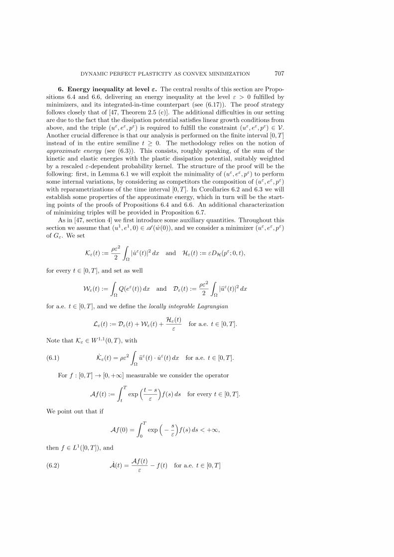
DYNAMIC PERFECT PLASTICITY AS CONVEX MINIMIZATION 707
6. Energy inequality at level \bfitvarepsilon . The central results of this section are Propo-sitions 6.4 and 6.6, delivering an energy inequality at the level \varepsilon > 0 fulfilled byminimizers, and its integrated-in-time counterpart (see (6.17)). The proof strategyfollows closely that of [47, Theorem 2.5 (c)]. The additional difficulties in our settingare due to the fact that the dissipation potential satisfies linear growth conditions fromabove, and the triple (u\varepsilon , e\varepsilon , p\varepsilon ) is required to fulfill the constraint (u\varepsilon , e\varepsilon , p\varepsilon ) \in \scrV .Another crucial difference is that our analysis is performed on the finite interval [0, T ]instead of in the entire semiline t \geq 0. The methodology relies on the notion ofapproximate energy (see (6.3)). This consists, roughly speaking, of the sum of thekinetic and elastic energies with the plastic dissipation potential, suitably weightedby a rescaled \varepsilon -dependent probability kernel. The structure of the proof will be thefollowing: first, in Lemma 6.1 we will exploit the minimality of (u\varepsilon , e\varepsilon , p\varepsilon ) to performsome internal variations, by considering as competitors the composition of (u\varepsilon , e\varepsilon , p\varepsilon )with reparametrizations of the time interval [0, T ]. In Corollaries 6.2 and 6.3 we willestablish some properties of the approximate energy, which in turn will be the start-ing points of the proofs of Propositions 6.4 and 6.6. An additional characterizationof minimizing triples will be provided in Proposition 6.7.
As in [47, section 4] we first introduce some auxiliary quantities. Throughout thissection we assume that (u1, e1, 0) \in A ( \.w(0)), and we consider a minimizer (u\varepsilon , e\varepsilon , p\varepsilon )of G\varepsilon . We set
\scrK \varepsilon (t) :=\rho \varepsilon 2
2
\int
\Omega
| \.u\varepsilon (t)| 2 dx and \scrH \varepsilon (t) := \varepsilon D\scrH (p\varepsilon ; 0, t),
for every t \in [0, T ], and set as well
\scrW \varepsilon (t) :=
\int
\Omega
Q(e\varepsilon (t)) dx and \scrD \varepsilon (t) :=\rho \varepsilon 2
2
\int
\Omega
| \"u\varepsilon (t)| 2 dx
for a.e. t \in [0, T ], and we define the locally integrable Lagrangian
\scrL \varepsilon (t) := \scrD \varepsilon (t) +\scrW \varepsilon (t) +\scrH \varepsilon (t)
\varepsilon for a.e. t \in [0, T ].
Note that \scrK \varepsilon \in W 1,1(0, T ), with
(6.1) \.\scrK \varepsilon (t) = \rho \varepsilon 2\int
\Omega
\"u\varepsilon (t) \cdot \.u\varepsilon (t) dx for a.e. t \in [0, T ].
For f : [0, T ] \rightarrow [0,+\infty ] measurable we consider the operator
\scrA f(t) :=\int T
t
exp\Bigl( t - s
\varepsilon
\Bigr) f(s) ds for every t \in [0, T ].
We point out that if
\scrA f(0) =\int T
0
exp\Bigl( - s
\varepsilon
\Bigr) f(s) ds < +\infty ,
then f \in L1([0, T ]), and
(6.2) \.\scrA (t) =\scrA f(t)\varepsilon
- f(t) for a.e. t \in [0, T ]

708 ELISA DAVOLI AND ULISSE STEFANELLI
satisfies \.\scrA \in L1(0, T ). In other words, if \scrA f(0) < +\infty , then \scrA f \in W 1,1([0, T ]).A direct computation yields
\scrA 2f(t) := \scrA (\scrA f)(t) =\int T
t
exp\Bigl( t - s
\varepsilon
\Bigr) (s - t)f(s) ds for every t \in [0, T ]
and
\scrA 2f(0) =
\int T
0
exp\Bigl( - s
\varepsilon
\Bigr) sf(s) ds.
For every \varepsilon > 0 the approximate energy \scrE \varepsilon is defined as
(6.3) \scrE \varepsilon (t) := \scrK \varepsilon (t) +\scrA 2\scrW \varepsilon (t) +1
\varepsilon \scrA 2\scrH \varepsilon (t) for every t \in [0, T ].
While the Lagrangian \scrL \varepsilon is given by the sum of the inertial term, the elasticenergy, and the dissipation, the approximate energy features the kinetic energy asso-ciated with the model, and an integrated version of the sum of the elastic energy andthe plastic dissipation potential, weighted by a suitably rescaled probability kernel.The presence of the third term in the right-hand side of (6.3) is a key difference withrespect to [47] and is needed due to the linear growth assumptions on the plastic dis-sipation potential in our setting. Indeed, in the case in which the dissipation potentialis quadratic, the associated estimates simplify, and it is thus possible to control thisquantity without adding the dissipative term to the approximate energy (see Defini-tion 4.2 and Proposition 4.4 in [47]). This is not the case in the situation in which thedissipation potential grows only linearly (see (4.8) in [47]). The term \scrA 2\scrH \varepsilon is addedto the approximate energy in order to overcome this technical difficulty.
We start by proving a preliminary inequality involving the quantities \scrD \varepsilon , \scrK \varepsilon , and\scrL \varepsilon .
Lemma 6.1. Let (u1, e1, 0) \in A ( \.w(0)), and let (u\varepsilon , e\varepsilon , p\varepsilon ) be a minimizer of G\varepsilon .Then,
\int T
0
exp\Bigl( - s
\varepsilon
\Bigr) (\varepsilon \.g(s) - g(s))\scrL \varepsilon (s) ds - 4\varepsilon
\int T
0
exp\Bigl( - s
\varepsilon
\Bigr) \.g(s)\scrD \varepsilon (s) ds
- \varepsilon
\int T
0
exp\Bigl( - s
\varepsilon
\Bigr) \"g(s) \.\scrK \varepsilon (s) ds+ \varepsilon 3\rho
\int T
0
\int
\Omega
exp\Bigl( - s
\varepsilon
\Bigr) \"u\varepsilon (s) \cdot ( \.w(s)g(s))\cdot \cdot dx ds
+ \varepsilon
\int T
0
\int
\Omega
exp\Bigl( - s
\varepsilon
\Bigr) \BbbC e\varepsilon (s) : E \.w(s)g(s) dx ds
+ \varepsilon
\int T
0
\int
\Omega
exp\Bigl( - s
\varepsilon
\Bigr) \BbbC e\varepsilon (s) : (e1 - E \.w(0))s \.g(0) dx ds \geq 0
for every g \in C2([0, T ]) such that g(0) = 0 and g(t) \geq 0 for every t \in [0, T ].
Proof. We argue as in [47, Proposition 4.4], and for every \delta > 0 we consider themap
\varphi \delta (t) := t - \delta \varepsilon g(t) for every t \in [0, T ].
For \delta small, \varphi \delta is a C2 diffeomorphism from [0, T ] to [0, \varphi \delta (T )], with inverse \psi \delta :[0, \varphi \delta (T )] \rightarrow [0, T ] satisfying
\psi \delta (t) := t+ \delta \varepsilon g(\psi \delta (t)) for every t \in [0, T ].

DYNAMIC PERFECT PLASTICITY AS CONVEX MINIMIZATION 709
We define the triple
\~u\varepsilon (t) := u\varepsilon (\varphi \delta (t)) + t\delta \varepsilon \.g(0)u1 + w(t) - w(\varphi \delta (t)) - t\delta \varepsilon \.g(0) \.w(0),
\~p\varepsilon (t) := p\varepsilon (\varphi \delta (t))
for every t \in [0, T ], and
\~e\varepsilon (t) := e\varepsilon (\varphi \delta (t)) + t\delta \varepsilon \.g(0)e1 + Ew(t) - Ew(\varphi \delta (t)) - t\delta \varepsilon \.g(0)E \.w(0)
for every t \in [0, T ]. Since (\~u\varepsilon , \~e\varepsilon , \~p\varepsilon ) \in \scrV , by the minimality of (u\varepsilon , e\varepsilon , p\varepsilon ) there holds
(6.4) lim sup\delta \rightarrow 0
G\varepsilon (\~u\varepsilon , \~e\varepsilon , \~p\varepsilon ) - G\varepsilon (u
\varepsilon , e\varepsilon , p\varepsilon )
\delta \geq 0.
We make the preliminary observation that
\.\~u\varepsilon (t) = \.u\varepsilon (\varphi \delta (t)) \.\varphi \delta (t) + \delta \varepsilon \.g(0)u1 + \.w(t) - \.w(\varphi \delta (t)) \.\varphi \delta (t) - \delta \varepsilon \.g(0) \.w(0)
for every t \in [0, T ], and
\"\~u\varepsilon (t) = \"u\varepsilon (\varphi \delta (t))( \.\varphi \delta (t))2 + \.u\varepsilon (\varphi \delta (t)) \"\varphi \delta (t) + \"w(t) - \"w(\varphi \delta (t))( \.\varphi \delta (t))
2 - \.w(\varphi \delta (t)) \"\varphi \delta (t)
for a.e. t \in [0, T ]. Therefore, a change of variable in inequality (6.4) yields
lim sup\delta \rightarrow 0
1
\delta
\Bigl\ \int \varphi \delta (T )
0
\.\psi \delta (t) exp\Bigl( - \psi \delta (t)
\varepsilon
\Bigr) \Bigl[ \varepsilon 2\rho 2
\int
\Omega
| \"u\varepsilon (t)( \.\varphi \delta (\psi \delta (t)))2
+ \.u\varepsilon (t) \"\varphi \delta (\psi \delta (t)) + \"w(\psi \delta (t)) - \"w(t)( \.\varphi \delta (\psi \delta (t)))2 - \.w(t) \"\varphi \delta (\psi \delta (t))| 2 dx
+
\int
\Omega
Q\bigl( e\varepsilon (t) + \psi \delta (t)\delta \varepsilon \.g(0)e
1 + Ew(\psi \delta (t)) - Ew(t) - \psi \delta (t)\delta \varepsilon \.g(0)E \.w(0)\bigr) dx\Bigr] dt
- \int T
0
exp\Bigl( - t
\varepsilon
\Bigr) \Bigl[ \varepsilon 2\rho 2
\int
\Omega
| \"u\varepsilon (t)| 2 dx+
\int
\Omega
Q(e\varepsilon (t)) dx\Bigr] dt
+ \varepsilon (D\scrH (exp( - \cdot /\varepsilon ); \~p\varepsilon ; 0, T ) - D\scrH (exp( - \cdot /\varepsilon ); p\varepsilon ; 0, T ))\Bigr\ \geq 0,
which in turn, since \varphi \delta (T ) \leq T , implies
lim sup\delta \rightarrow 0
1
\delta
\Bigl\ \int \varphi \delta (T )
0
\.\psi \delta (t) exp\Bigl( - \psi \delta (t)
\varepsilon
\Bigr) \Bigl[ \varepsilon 2\rho 2
\int
\Omega
| \"u\varepsilon (t)( \.\varphi \delta (\psi \delta (t)))2(6.5)
+ \.u\varepsilon (t) \"\varphi \delta (\psi \delta (t)) + \"w(\psi \delta (t)) - \"w(t)( \.\varphi \delta (\psi \delta (t)))2 - \.w(t) \"\varphi \delta (\psi \delta (t))| 2 dx
+
\int
\Omega
Q(e\varepsilon (t) + \psi \delta (t)\delta \varepsilon \.g(0)e1 + Ew(\psi \delta (t)) - Ew(t) - \psi \delta (t)\delta \varepsilon \.g(0)E \.w(0)) dx
\Bigr] dt
- \int \varphi \delta (T )
0
exp\Bigl( - t
\varepsilon
\Bigr) \Bigl[ \varepsilon 2\rho 2
\int
\Omega
| \"u\varepsilon (t)| 2 dx+
\int
\Omega
Q(e\varepsilon (t)) dx\Bigr] dt
+ \varepsilon (D\scrH (exp( - \cdot /\varepsilon ); \~p\varepsilon ; 0, T ) - D\scrH (exp( - \cdot /\varepsilon ); p\varepsilon ; 0, \varphi \delta (T )))\Bigr\ \geq 0.

710 ELISA DAVOLI AND ULISSE STEFANELLI
The inertial terms satisfy
lim sup\delta \rightarrow 0
1
\delta
\Bigl\ \int \varphi \delta (T )
0
\.\psi \delta (t) exp\Bigl( - \psi \delta (t)
\varepsilon
\Bigr) \Bigl[ \varepsilon 2\rho 2
\int
\Omega
| \"u\varepsilon (t)( \.\varphi \delta (\psi \delta (t)))2(6.6)
+ \.u\varepsilon (t) \"\varphi \delta (\psi \delta (t)) + \"w(\psi \delta (t)) - \"w(t)( \.\varphi \delta (\psi \delta (t)))2 - \.w(t) \"\varphi \delta (\psi \delta (t))| 2
\Bigr] dx dt
- \varepsilon 2\rho
2
\int \varphi \delta (T )
0
exp\Bigl( - t
\varepsilon
\Bigr) \int
\Omega
| \"u\varepsilon (t)| 2 dx dt\Bigr\
=\varepsilon 2\rho
2
\int T
0
(\varepsilon \.g(t) - g(t)) exp\Bigl( - t
\varepsilon
\Bigr) \int
\Omega
| \"u\varepsilon (t)| 2 dx dt
+ \varepsilon 3\rho
\int T
0
exp\Bigl( - t
\varepsilon
\Bigr) \int
\Omega
\"u\varepsilon (t) \cdot \Bigl( - 2\"u\varepsilon (t) \.g(t) - \.u\varepsilon (t)\"g(t)+
...w(t)g(t)
+ 2 \"w(t) \.g(t)+ \.w(t)\"g(t)\Bigr) dx dt.
This latter inequality follows by the dominated convergence theorem, by the fact thatthe left-hand side coincides with the integral between 0 and \varphi \delta (T ) of the incrementalratio between 0 and \delta of the function
\.\psi \delta (t) exp\Bigl( - \psi \delta (t)
\varepsilon
\Bigr) \Bigl[ \varepsilon 2\rho 2
\int
\Omega
| \"u\varepsilon (t)( \.\varphi \delta (\psi \delta (t)))2 + \.u\varepsilon (t) \"\varphi \delta (\psi \delta (t)) + \"w(\psi \delta (t))
- \"w(t)( \.\varphi \delta (\psi \delta (t)))2 - \.w(t) \"\varphi \delta (\psi \delta (t))| 2
\Bigr] dx,
and by the identities
\partial
\partial \delta
\Bigl( \.\psi \delta (t) exp
\Bigl( - \psi \delta (t)
\varepsilon
\Bigr) \Bigr) \bigm| \bigm| \bigm| \delta =0
= (\varepsilon \.g(t) - g(t)) exp\Bigl( - t
\varepsilon
\Bigr) ,
\partial
\partial \delta \psi \delta (t)
\bigm| \bigm| \bigm| \delta =0
= \varepsilon g(t),
\partial
\partial \delta ( \.\varphi \delta (\psi \delta (t)))
2\bigm| \bigm| \bigm| \delta =0
= - 2\varepsilon \.g(t),
\partial
\partial \delta \"\varphi \delta (\psi \delta (t))
\bigm| \bigm| \bigm| \delta =0
= - \varepsilon \"g(t)
for every t \in [0, T ], and
\partial
\partial \delta
\Bigl( \int
\Omega
| \"u\varepsilon (t)( \.\varphi \delta (\psi \delta (t)))2 + \.u\varepsilon (t) \"\varphi \delta (\psi \delta (t)) + \"w(\psi \delta (t))
- \"w(t)( \.\varphi \delta (\psi \delta (t)))2 - \.w(t) \"\varphi \delta (\psi \delta (t))| 2 dx
\Bigr) \bigm| \bigm| \bigm| \delta =0
= 2\varepsilon
\int
\Omega
\"u\varepsilon (t) \cdot \Bigl( - 2\"u\varepsilon (t) \.g(t) - \.u\varepsilon (t)\"g(t) +
...w(t)g(t) + 2 \"w(t) \.g(t) + \.w(t)\"g(t)
\Bigr) dx
for a.e. t \in [0, T ]. Analogously,
\partial
\partial \delta
\int
\Omega
Q(e\varepsilon (t) + \psi \delta (t)\delta \varepsilon \.g(0)e1 + Ew(\psi \delta (t)) - Ew(t) - \psi \delta (t)\delta \varepsilon \.g(0)E \.w(0)) dx
\bigm| \bigm| \bigm| \delta =0
= \varepsilon
\int
\Omega
\BbbC e\varepsilon (t) :\Bigl( E \.w(t)g(t) + t \.g(0)e1 - t \.g(0)E \.w(0)
\Bigr) dx,

DYNAMIC PERFECT PLASTICITY AS CONVEX MINIMIZATION 711
for a.e. t \in [0, T ], and hence
lim sup\delta \rightarrow 0
1
\delta
\Bigl\ \int \varphi \delta (T )
0
\.\psi \delta (t) exp\Bigl( - \psi \delta (t)
\varepsilon
\Bigr) \int
\Omega
Q\Bigl( e\varepsilon (t) + \psi \delta (t)\delta \varepsilon \.g(0)e
1 + Ew(\psi \delta (t))
- Ew(t) - \psi \delta (t)\delta \varepsilon \.g(0)E \.w(0)\Bigr) dx dt -
\int \varphi \delta (T )
0
exp\Bigl( - t
\varepsilon
\Bigr) \int
\Omega
Q(e\varepsilon (t)) dx dt\Bigr\
=
\int T
0
(\varepsilon \.g(t) - g(t)) exp\Bigl( - t
\varepsilon
\Bigr) \int
\Omega
Q(e\varepsilon (t)) dx dt
+ \varepsilon
\int T
0
exp\Bigl( - t
\varepsilon
\Bigr) \int
\Omega
\BbbC e\varepsilon (t) :\Bigl( E \.w(t)g(t) + t \.g(0)e1 - t \.g(0)E \.w(0)
\Bigr) dx dt.
(6.7)
To complete the proof of the lemma it remains to study the asymptotic behavior ofthe dissipation as \delta \rightarrow 0. Fix \lambda > 0, and let 0 \leq t0 < t1 < \cdot \cdot \cdot < tm \leq T be such that
D\scrH (exp( - \cdot /\varepsilon ); \~p\varepsilon ; 0, T ) \leq m\sum
i=1
exp
\biggl( - ti\varepsilon
\biggr) \scrH (\~p\varepsilon (ti) - \~p\varepsilon (ri - 1)) + \lambda .
For i = 1, . . . ,m, let si \in [0, \varphi \delta (T )] be such that ti = \psi \delta (si). There holds
m\sum
i=1
exp
\biggl( - ti\varepsilon
\biggr) \scrH (\~p\varepsilon (ti) - \~p\varepsilon (ri - 1)) =
m\sum
i=1
exp
\biggl( - \psi \delta (si)
\varepsilon
\biggr) \scrH (p\varepsilon (si) - p\varepsilon (si - 1))
=m\sum
i=1
exp\Bigl( - si\varepsilon
\Bigr) \scrH (p\varepsilon (si) - p\varepsilon (si - 1))
+m\sum
i=1
exp\Bigl( - si\varepsilon
\Bigr) \Bigl[ exp ( - \delta g(\psi \delta (si))) - 1
\Bigr] \scrH (p\varepsilon (si) - p\varepsilon (si - 1))
\leq D\scrH (exp( - \cdot /\varepsilon ); p\varepsilon ; 0, \varphi \delta (T ))
- \delta
m\sum
i=1
exp\Bigl( - si\varepsilon
\Bigr) g(\psi \delta (si))\scrH (p\varepsilon (si) - p\varepsilon (si - 1)) + O(\delta 2)
= D\scrH (exp( - \cdot /\varepsilon ); p\varepsilon ; 0, \varphi \delta (T ))
- \delta m\sum
i=1
exp\Bigl( - si\varepsilon
\Bigr) g(si)\scrH (p\varepsilon (si) - p\varepsilon (si - 1)) + O(\delta 2).
Thus,
D\scrH (exp( - \cdot /\varepsilon ); \~p\varepsilon ; 0, T ) \leq D\scrH (exp( - \cdot /\varepsilon ); p\varepsilon ; 0, \varphi \delta (T )) + \lambda
- \delta
m\sum
i=1
exp\Bigl( - si\varepsilon
\Bigr) g(si)\scrH (p\varepsilon (si) - p\varepsilon (si - 1)) + O(\delta 2).
By considering finer and finer refinements of \ t0, . . . , tm\ , in view of the definition of\^D\scrH (see (2.9)), and by the arbitrariness of \lambda we conclude that
D\scrH (exp( - \cdot /\varepsilon ); \~p\varepsilon ; 0, T )(6.8)
\leq D\scrH (exp( - \cdot /\varepsilon ); p\varepsilon ; 0, \varphi \delta (T )) + \delta \^D\scrH ( - exp( - \cdot /\varepsilon )g(\cdot ); 0, \varphi \delta (T )) + O(\delta 2).

712 ELISA DAVOLI AND ULISSE STEFANELLI
By (6.8) and [21, Theorem 4.5] we obtain
lim sup\delta \rightarrow 0
\varepsilon
\delta
\bigl( D\scrH (exp( - \cdot /\varepsilon ); \~p\varepsilon ; 0, T ) - D\scrH (exp( - \cdot /\varepsilon ); p\varepsilon ; 0, \varphi \delta (T ))
\bigr) (6.9)
\leq lim sup\delta \rightarrow 0
\varepsilon \^D\scrH ( - exp( - \cdot /\varepsilon )g(\cdot ); 0, \varphi \delta (T )) = lim sup\delta \rightarrow 0
- \varepsilon PMS
\int \varphi \delta (T )
0
exp\Bigl( - t
\varepsilon
\Bigr) g(t) dD\scrH (p\varepsilon ; 0, t)
= - lim inf\delta \rightarrow 0
\Bigl\ \varepsilon g(\varphi \delta (T )) exp
\Bigl( - \varphi \delta (T )
\varepsilon
\Bigr) D\scrH (p\varepsilon ; 0, \varphi \delta (T ))
- \int \varphi \delta (T )
0
(\varepsilon \.g(t) - g(t)) exp\Bigl( - t
\varepsilon
\Bigr) D\scrH (p\varepsilon ; 0, t) dt
\Bigr\
\leq \int T
0
(\varepsilon \.g(t) - g(t)) exp\Bigl( - t
\varepsilon
\Bigr) D\scrH (p\varepsilon ; 0, t) dt.
The thesis follows by combining (6.1), (6.5)--(6.7), and (6.9) and by the definitions of\scrK \varepsilon , \scrD \varepsilon , and \scrL \varepsilon .Setting
R\varepsilon (t) := - \varepsilon \int
\Omega
\BbbC e\varepsilon (t) :\bigl( e1 - E \.w(0)
\bigr) dx,(6.10)
\~R\varepsilon (t) := - \varepsilon 3\rho \int
\Omega
\"u\varepsilon (t) \cdot ...w(t) dx - \varepsilon
\int
\Omega
\BbbC e\varepsilon (t) : E \.w(t) dx,(6.11)
\^R\varepsilon (t) := - 2\varepsilon 3\rho
\int
\Omega
\"u\varepsilon (t) \cdot \"w(t) dx,(6.12)
\r R\varepsilon (t) := - \varepsilon 3\rho \int
\Omega
\"u\varepsilon (t) \cdot \.w(t) dx,(6.13)
for a.e. t \in [0, T ], and choosing g(t) = t in Lemma 6.1, the same approximationargument as in [47, Corollary 4.5] yields the following.
Corollary 6.2. Let (u1, e1, 0) \in A ( \.w(0)), and let (u\varepsilon , e\varepsilon , p\varepsilon ) be a minimizer ofG\varepsilon . Then
\varepsilon \scrA \scrL \varepsilon (0) - \scrA 2\scrL \varepsilon (0) - 4\varepsilon \scrA \scrD \varepsilon (0) \geq \scrA 2R\varepsilon (0) +\scrA 2 \~R\varepsilon (0) +\scrA \^R\varepsilon (0).
Finally, by considering the sequence of maps g\delta : [0, T ] \rightarrow [0,+\infty ) defined as
g\delta (s) :=
\left\
0 if s \leq t,(s - t)2
2\delta if t < s < t+ \delta ,
s - t - \delta 2 if s \geq t+ \delta
in Lemma 6.1, and by letting \delta go to zero, we deduce the following inequality.
Corollary 6.3. Let (u1, e1, 0) \in A ( \.w(0)), and let (u\varepsilon , e\varepsilon , p\varepsilon ) be a minimizer ofG\varepsilon . Then
\varepsilon \scrA \scrL \varepsilon (t) - \scrA 2\scrL \varepsilon (t) - 4\varepsilon \scrA \scrD \varepsilon (t) - \varepsilon \.\scrK \varepsilon (t) \geq \scrA 2 \~R\varepsilon (t) +\scrA \^R\varepsilon (t) + \r R\varepsilon (t)
for a.e. t \in [0, T ].

DYNAMIC PERFECT PLASTICITY AS CONVEX MINIMIZATION 713
We are now in a position to prove an energy inequality at the level \varepsilon > 0.
Proposition 6.4 (energy inequality). Let (u1, e1, 0) \in A ( \.w(0)), and let(u\varepsilon , e\varepsilon , p\varepsilon ) be a minimizer of G\varepsilon . Then
\scrE \varepsilon (t)\varepsilon 2
- \rho
\int
\Omega
\.u\varepsilon (t) \cdot \.w(t) dx+\scrA 2 \~R\varepsilon (t)
\varepsilon 2+
\scrA \^R\varepsilon (t)
\varepsilon 2+
\scrA \~R\varepsilon (t)
\varepsilon
\leq \scrE \varepsilon (0)\varepsilon 2
- \rho
\int
\Omega
u1 \cdot \.w(0) dx+\scrA 2 \~R\varepsilon (0)
\varepsilon 2+
\scrA \^R\varepsilon (0)
\varepsilon 2+
\scrA \~R\varepsilon (0)
\varepsilon
- \rho
\int t
0
\int
\Omega
\.u\varepsilon (s) \cdot \"w(s) dx ds+\int t
0
\~R\varepsilon (s)
\varepsilon ds -
\int t
0
\^R\varepsilon (s)
\varepsilon 2ds.
Proof. By the definition of the approximate energy (see (6.3)) there holds
\scrE \varepsilon (t) := \scrK \varepsilon (t) +\scrA 2(\scrL \varepsilon - \scrD \varepsilon )(t)
for every t \in [0, T ], which by (6.2) implies
\.\scrE \varepsilon (t) = \.\scrK \varepsilon (t) +\scrA 2\scrL \varepsilon (t)
\varepsilon - \scrA 2\scrD \varepsilon (t)
\varepsilon - \scrA \scrL \varepsilon (t) +\scrA \scrD \varepsilon (t)
for a.e. t \in [0, T ]. On the one hand, in view of Corollary 6.3, we obtain the estimate
\.\scrE \varepsilon (t) \leq - \scrA 2\scrD \varepsilon (t)\varepsilon
- 3\scrA \scrD \varepsilon (t) - \scrA 2 \~R\varepsilon (t)
\varepsilon - \scrA \^R\varepsilon (t)
\varepsilon -
\r R\varepsilon (t)
\varepsilon
\leq - \scrA 2 \~R\varepsilon (t)
\varepsilon - \scrA \^R\varepsilon (t)
\varepsilon -
\r R\varepsilon (t)
\varepsilon (6.14)
for a.e. t \in [0, T ]. On the other hand, by (6.2),
(6.15) - \r R\varepsilon (t)
\varepsilon 3= \rho \Bigl( \int
\Omega
\.u\varepsilon (t) \cdot \.w(t) dx\Bigr) . - \rho
\int
\Omega
\.u\varepsilon (t) \cdot \"w(t) dx,
and
- \scrA 2 \~R\varepsilon (t)
\varepsilon 3 - \scrA \^R\varepsilon (t)
\varepsilon 3=\Bigl( - \scrA 2 \~R\varepsilon (t)
\varepsilon 2 - \scrA \^R\varepsilon (t)
\varepsilon 2
\Bigr) . - \scrA \~R\varepsilon (t)
\varepsilon 2 -
\^R\varepsilon (t)
\varepsilon 2
=\Bigl( - \scrA 2 \~R\varepsilon (t)
\varepsilon 2 - \scrA \^R\varepsilon (t)
\varepsilon 2 - \scrA \~R\varepsilon (t)
\varepsilon
\Bigr) . -
\~R\varepsilon (t)
\varepsilon -
\^R\varepsilon (t)
\varepsilon 2(6.16)
for a.e. t \in [0, T ]. By combining (6.14)--(6.16) we deduce
\Bigl( \scrE \varepsilon (t)\varepsilon 2
- \rho
\int
\Omega
\.u\varepsilon (t) \cdot \.w(t) dx+\scrA 2 \~R\varepsilon (t)
\varepsilon 2+
\scrA \^R\varepsilon (t)
\varepsilon 2+
\scrA \~R\varepsilon (t)
\varepsilon
\Bigr) .
\leq - \rho \int
\Omega
\.u\varepsilon (t) \cdot \"w(t) dx+\~R\varepsilon (t)
\varepsilon -
\^R\varepsilon (t)
\varepsilon 2
for a.e. t \in [0, T ]. An integration in time in [0, T ] yields the thesis.
The same argument in [47, Lemma 6.1] provides the following technical result.

714 ELISA DAVOLI AND ULISSE STEFANELLI
Lemma 6.5. Let \ell and m be two nonnegative functions in L1(0, T ) such that
\scrA 2\ell (t) \leq m(t) for a.e. t \in [0, T ].
Then, for every a > 0 and every \delta \in (0, 1), there holds
\Bigl( \int \delta a
0
s exp\Bigl( - s
\varepsilon
\Bigr) ds\Bigr) \int t+a
t+\delta a
\ell (s) ds \leq \int t+a
t
m(s) ds
for every t \in [0, T - a].
In view of Proposition 6.4 and Lemma 6.5, we obtain an integrated-in-time versionof the \varepsilon -energy inequality.
Proposition 6.6 (integral energy inequality). Let (u1, e1, 0) \in A ( \.w(0)), and let(u\varepsilon , e\varepsilon , p\varepsilon ) be a minimizer of G\varepsilon . Then, for every a > 0 and \delta \in (0, 1), there holds
\Bigl( 1
\varepsilon 2
\int \delta a
0
s exp\Bigl( - s
\varepsilon
\Bigr) ds\Bigr) \int t+a
t+\delta a
\Bigl( \int
\Omega
Q(e\varepsilon (s)) dx+D\scrH (p\varepsilon ; 0, s)\Bigr) ds
(6.17)
+\rho
2
\int t+a
t
\int
\Omega
| \.u\varepsilon (s)| 2 dx ds
- \rho
\int t+a
t
\int
\Omega
\.u\varepsilon (s) \cdot \.w(s) dx ds \leq - \int t+a
t
\Bigl( \scrA 2 \~R\varepsilon (s)
\varepsilon 2+
\scrA \^R\varepsilon (s)
\varepsilon 2+
\scrA \~R\varepsilon (s)
\varepsilon
\Bigr) ds
+\scrE \varepsilon (0)a\varepsilon 2
- \rho a
\int
\Omega
u1 \cdot \.w(0) dx+ a\scrA 2 \~R\varepsilon (0)
\varepsilon 2+ a
\scrA \^R\varepsilon (0)
\varepsilon 2+ a
\scrA \~R\varepsilon (0)
\varepsilon
- \rho
\int t+a
t
\int \xi
0
\int
\Omega
\.u\varepsilon (s) \cdot \"w(s) dx ds d\xi +\int t+a
t
\int \xi
0
\~R\varepsilon (s)
\varepsilon ds d\xi -
\int t+a
t
\int \xi
0
\^R\varepsilon (s)
\varepsilon 2ds d\xi
for every t \in [0, T ].
Proof. Owing to Proposition 6.4 we can apply Lemma 6.5, with
\ell (t) :=\scrW \varepsilon (t)
\varepsilon 2+
\scrH \varepsilon (t)
\varepsilon 3,
and with
m(t) := - \scrK \varepsilon (t)\varepsilon 2
+ \rho
\int
\Omega
\.u\varepsilon (t) \cdot \.w(t) dx - \scrA 2 \~R\varepsilon (t)
\varepsilon 2 - \scrA \^R\varepsilon (t)
\varepsilon 2 - \scrA \~R\varepsilon (t)
\varepsilon
+\scrE \varepsilon (0)\varepsilon 2
- \rho
\int
\Omega
u1 \cdot \.w(0) dx+\scrA 2 \~R\varepsilon (0)
\varepsilon 2+
\scrA \^R\varepsilon (0)
\varepsilon 2+
\scrA \~R\varepsilon (0)
\varepsilon
- \rho
\int t
0
\int
\Omega
\.u\varepsilon (s) \cdot \"w(s) dx ds+\int t
0
\~R\varepsilon (s)
\varepsilon ds -
\int t
0
\^R\varepsilon (s)
\varepsilon 2ds
for a.e. t \in [0, T ]. The thesis follows by the definitions of \scrW \varepsilon , \scrH \varepsilon , and \scrK \varepsilon .We conclude this section by showing a further characterization of \varepsilon -minimizers.
Proposition 6.7 (weak energy equality). Let (u\varepsilon , e\varepsilon , p\varepsilon ) be a minimizer of G\varepsilon .

DYNAMIC PERFECT PLASTICITY AS CONVEX MINIMIZATION 715
Then,
\int T
0
\.\varphi (t)\Bigl[ \int
\Omega
Q\bigl( e\varepsilon (t)
\bigr) dx+ 2\varepsilon \rho
\int t
0
\int
\Omega
| \"u\varepsilon (s)| 2 dx ds+ \rho
2
\int
\Omega
| \.u\varepsilon (t)| 2 dx
(6.18)
+D\scrH (p\varepsilon ; 0, t)\Bigr] dt =
\int T
0
\.\varphi (t)
\int t
0
\int
\Omega
\BbbC e\varepsilon (s) : E \.w(s) dx ds dt
- 3\varepsilon 2\rho
2
\int T
0
\"\varphi (t)
\int t
0
\int
\Omega
| \"u\varepsilon (s)| 2 dx ds dt - \varepsilon 2\rho
\int T
0
\"\varphi (t)
\int
\Omega
\"u\varepsilon (t) \cdot ( \.w(t) - \.u\varepsilon (t)) dx dt
+ \rho
\int T
0
\int
\Omega
\.u\varepsilon (t) \cdot \partial t[ \.w(t)(\varphi (t) + 2\varepsilon \.\varphi (t))] dx dt - \varepsilon 2\rho
\int T
0
\int
\Omega
\"u\varepsilon (t) \cdot ...w(t)\varphi (t) dx dt
- \varepsilon \rho
\int T
0
\int
\Omega
\"\varphi (t)| \.u\varepsilon (t)| 2 dx dt+ 2\varepsilon \rho
\int T
0
\int
\Omega
\.u\varepsilon (t) \cdot \partial t[ \"w(t)(\varphi (t) + \varepsilon \.\varphi (t))] dx dt
for every \varphi \in C\infty c (0, T ).
This last result of this section relies on the argument developed in [38, Proposition4.1], which consists of comparing the energy associated to a minimizer (u\varepsilon , e\varepsilon , p\varepsilon ) ofG\varepsilon with that of a suitably rescaled triple (\~u\varepsilon , \~e\varepsilon , \~p\varepsilon ), obtained by composing (u\varepsilon , e\varepsilon , p\varepsilon )with a diffeomorphic reparametrization of [0, T ]. We postpone the proof of Proposition6.7 to Appendix A.
7. Proof of Theorem 2.3. For the reader's convenience, we subdivide the proofinto four steps. In Step 1, we deduce some first compactness properties for sequencesof minimizers of G\varepsilon satisfying the uniform energy estimate (5.42). In Step 2, we showthat the limit triples identified in Step 1 satisfy conditions (c1) and (c2). Step 3 relieson the inequalities at level \varepsilon > 0 proven in section 6, and it is devoted to the proofof the energy inequality (c3). Finally, in Step 4 we prove that the limit triples satisfythe first-order initial condition \.u(0) = u1.
Step 1. Having established the uniform estimate (5.42), we are now ready toprove Theorem 2.3. For every \varepsilon > 0, let (u\varepsilon , e\varepsilon , p\varepsilon ) be a minimizer of G\varepsilon satisfying(5.42). Since p\varepsilon (0) = p0 for every \varepsilon > 0, by a generalization of Helly's theorem [11,Theorem 7.2] there exists p \in BV (0, T ;\scrM b(\Omega \cup \Gamma 0;\BbbM 3\times 3
D )) such that
p\varepsilon (t)\rightharpoonup p(t) weakly* in \scrM b(\Omega \cup \Gamma 0;\BbbM 3\times 3D ) for every t \in [0, T ],(7.1)
D\scrH (p; 0, T ) \leq lim inf\varepsilon \rightarrow 0
D\scrH (p\varepsilon ; 0, T ).(7.2)
In addition, (5.42) yields the existence of maps u \in W 1,2(0, T ;L2(\Omega ;\BbbR 3)) and e \in L2(0, T ;L2(\Omega ;\BbbM 3\times 3
sym)) such that, up to subsequences,
u\varepsilon \rightharpoonup u weakly in W 1,2(0, T ;L2(\Omega ;\BbbR 3)),(7.3)
e\varepsilon \rightharpoonup e weakly in L2(0, T ;L2(\Omega ;\BbbM 3\times 3sym)).(7.4)
In particular, by (7.3) and the embedding of W 1,2(0, T ;L2(\Omega ;\BbbR 3)) intoCw([0, T ];L
2(\Omega ;\BbbR 3)), there holds
(7.5) u\varepsilon (t)\rightharpoonup u(t) weakly in L2(\Omega ;\BbbR 3) for every t \in [0, T ]
and u(0) = u0. In view of (7.1), (7.4), and (7.5), we obtain that
(7.6) e\varepsilon (t)\rightharpoonup e(t) weakly in \scrD \prime (\Omega ;\BbbM 3\times 3sym) for every t \in [0, T ].

716 ELISA DAVOLI AND ULISSE STEFANELLI
By (7.1), (7.5), (7.6), and Fatou's lemma for a.e. t \in [0, T ], there exists a t-dependent subsequence \ \varepsilon t\ such that
e\varepsilon t(t)\rightharpoonup e(t) weakly in L2(\Omega ;\BbbM 3\times 3sym),(7.7)
u\varepsilon t(t)\rightharpoonup \ast u(t) weakly* in BD(\Omega ).(7.8)
The fact that p satisfies the Dirichlet condition on \Gamma 0 for a.e. t \in [0, T ] follows byarguing as in [11, Lemma 2.1].
Step 2. Let v \in C\infty c ((0, T )\times \Omega ;\BbbR 3). For \lambda > 0, we have that
\Bigl( u\varepsilon + \lambda exp
\Bigl( t\varepsilon
\Bigr) v, e\varepsilon + \lambda exp
\Bigl( t\varepsilon
\Bigr) Ev, p\varepsilon
\Bigr) \in \scrV ,
and thus by the minimality of (u\varepsilon , e\varepsilon , p\varepsilon ),
1
\lambda
\biggl( G\varepsilon
\biggl( u\varepsilon + \lambda exp
\biggl( t
\varepsilon
\biggr) v, e\varepsilon + \lambda exp
\biggl( t
\varepsilon
\biggr) Ev, p\varepsilon
\biggr) - G\varepsilon (u
\varepsilon , e\varepsilon , p\varepsilon )
\biggr) \geq 0.
By the arbitrariness of \lambda , considering the limsup of the inequality above as \lambda \rightarrow 0, wededuce
\rho
\int T
0
\int
\Omega
\"u\varepsilon \cdot (v + 2\varepsilon \.v + \varepsilon 2\"v) dx dt+
\int T
0
\int
\Omega
\BbbC e\varepsilon : Ev dx dt \geq 0
for every v \in C\infty c ((0, T )\times \Omega ;\BbbR 3). Analogously, by considering variations of the form
\Bigl( u\varepsilon - \lambda exp
\Bigl( t\varepsilon
\Bigr) v, e\varepsilon - \lambda exp
\Bigl( t\varepsilon
\Bigr) Ev, p\varepsilon
\Bigr) ,
for \lambda > 0 and v \in C\infty c ((0, T )\times \Omega ;\BbbR 3), we obtain
(7.9) \rho
\int T
0
\int
\Omega
\"u\varepsilon \cdot (v + 2\varepsilon \.v + \varepsilon 2\"v) dx dt+
\int T
0
\int
\Omega
\BbbC e\varepsilon : Ev dx dt = 0
for every v \in C\infty c ((0, T )\times \Omega ;\BbbR 3). Integrating by parts with respect to time, (7.3) and
(7.4) yield
- \rho \int T
0
\int
\Omega
\.u \cdot \.v dx dt+\int T
0
\int
\Omega
\BbbC e : Ev dx dt = 0
for every v \in C\infty c ((0, T )\times \Omega ;\BbbR 3), that is,
(7.10) \rho \"u - div\BbbC e = 0
in the sense of distributions. Since the same procedure applies to everyv \in C\infty
c (0, T ;C\infty (\=\Omega ;\BbbR 3)) with v = 0 on \Gamma 0 for every t \in [0, T ], we also obtain
(7.11) \BbbC e\nu = 0 on \partial \Omega \setminus \Gamma 0.
Let now q \in C\infty c (0, T ;L2(\Omega ;\BbbM 3\times 3
D )), \lambda > 0, and consider the test triple
\Bigl( u\varepsilon , e\varepsilon - \lambda exp
\Bigl( t\varepsilon
\Bigr) q, p\varepsilon + \lambda exp
\Bigl( t\varepsilon
\Bigr) q\Bigr) .
On the one hand, by the minimality of (u\varepsilon , e\varepsilon , p\varepsilon ),
(7.12)1
\lambda
\biggl( G\varepsilon
\biggl( u\varepsilon , e\varepsilon - \lambda exp
\biggl( t
\varepsilon
\biggr) q, p\varepsilon + \lambda exp
\Bigl( t\varepsilon
\Bigr) q
\biggr) - G\varepsilon (u
\varepsilon , e\varepsilon , p\varepsilon )
\biggr) \geq 0.

DYNAMIC PERFECT PLASTICITY AS CONVEX MINIMIZATION 717
On the other hand,
1
\lambda (D\scrH (exp( - \cdot /\varepsilon ); p\varepsilon + \lambda exp(\cdot /\varepsilon )q; 0, T ) - D\scrH (exp( - \cdot /\varepsilon ); p\varepsilon ; 0, T ))
\leq D\scrH (exp( - \cdot /\varepsilon ); exp(\cdot /\varepsilon )q; 0, T ),
and by the in-time regularity of q,
D\scrH (exp( - \cdot /\varepsilon ); exp(\cdot /\varepsilon )q; 0, T ) =\int T
0
exp\Bigl( - t
\varepsilon
\Bigr) \scrH \Bigl( 1\varepsilon exp
\Bigl( t\varepsilon
\Bigr) q(t) + exp
\Bigl( t\varepsilon
\Bigr) \.q(t)\Bigr)
\leq 1
\varepsilon
\int T
0
\scrH (q(t)) dt+
\int T
0
\scrH ( \.q(t)) dt.
Thus, (7.12) can be rewritten as
- \int T
0
\int
\Omega
\BbbC e\varepsilon : q dx dt+\int T
0
\scrH (q(t)) dt+ \varepsilon
\int T
0
\scrH ( \.q(t)) dt \geq 0
for every q \in C\infty c (0, T ;L2(\Omega ;\BbbM 3\times 3
D )), and by (7.4),
\int T
0
\int
\Omega
\BbbC e : q dx dt \leq \int T
0
\scrH (q(t)) dt
for every q \in C\infty c (0, T ;L2(\Omega ;\BbbM 3\times 3
D )). By approximation, the previous inequalityholds in particular by choosing q = M\chi I\chi B with M \in \BbbM 3\times 3
D , I and B Borel subsetsof (0, T ) and \Omega \cup \Gamma 0, respectively. Hence, we deduce that
(7.13) (\BbbC e(t))D \in \partial H(0)
for a.e. t \in [0, T ] and x \in \Omega .Step 3. It remains to show that the limit triple satisfies the energy inequality
(c3). We first fix a > 0 and \delta \in (0, 1), and we argue by passing to the limit as \varepsilon \rightarrow 0in (6.17). Since
lim\varepsilon \rightarrow 0
1
\varepsilon 2
\int \delta a
0
s exp\Bigl( - s
\varepsilon
\Bigr) ds = 1,
by (7.2), (7.3), and (7.4), we have
\int t+a
t+\delta a
\Bigl( \int
\Omega
Q(e(s)) dx+D\scrH (p; 0, s)\Bigr) ds+
\rho
2
\int t+a
t
\int
\Omega
| \.u(s)| 2 dx ds
(7.14)
- \rho
\int t+a
t
\int
\Omega
\.u(s) \cdot \.w(s) dx ds \leq - \rho a\int
\Omega
u1 \cdot \.w(0) dx
- \rho
\int t+a
t
\int \xi
0
\int
\Omega
\.u(s) \cdot \"w(s) dx ds d\xi
+ lim sup\varepsilon \rightarrow 0
\Bigl\ - \int t+a
t
\Bigl( \scrA 2 \~R\varepsilon (s)
\varepsilon 2+
\scrA \^R\varepsilon (s)
\varepsilon 2+
\scrA \~R\varepsilon (s)
\varepsilon
\Bigr) ds+
\scrE \varepsilon (0)a\varepsilon 2
+ a\scrA 2 \~R\varepsilon (0)
\varepsilon 2
+ a\scrA \^R\varepsilon (0)
\varepsilon 2+ a
\scrA \~R\varepsilon (0)
\varepsilon +
\int t+a
t
\int \xi
0
\~R\varepsilon (s)
\varepsilon ds d\xi -
\int t+a
t
\int \xi
0
\^R\varepsilon (s)
\varepsilon 2ds d\xi
\Bigr\ ,

718 ELISA DAVOLI AND ULISSE STEFANELLI
where \~R\varepsilon and \^R\varepsilon are the quantities defined in (6.11) and (6.12), respectively. By(5.42) there holds(7.15)
\bigm| \bigm| \bigm| \int t+a
t
\int \xi
0
\^R\varepsilon (s)
\varepsilon 2ds d\xi
\bigm| \bigm| \bigm| \leq Ca\varepsilon \| \"u\varepsilon \| L2(0,T ;L2(\Omega ;\BbbR 3))\| \"w\| L\infty (0,T ;L2(\Omega ;\BbbR 3)) \leq Ca\surd \varepsilon
and, analogously,
(7.16)\bigm| \bigm| \bigm| \int t+a
t
\int \xi
0
\~R\varepsilon (s)
\varepsilon ds d\xi +
\int t+a
t
\int \xi
0
\int
\Omega
\BbbC e\varepsilon (s) : E \.w(s) dx ds d\xi \bigm| \bigm| \bigm| \leq Ca\varepsilon
\surd \varepsilon
for every t \in [0, T ]. Thus, by (7.4)(7.17)
lim\varepsilon \rightarrow 0
\int t+a
t
\int \xi
0
\~R\varepsilon (s)
\varepsilon ds d\xi -
\int t+a
t
\int \xi
0
\^R\varepsilon (s)
\varepsilon 2ds d\xi = -
\int t+a
t
\int \xi
0
\int
\Omega
\BbbC e(s) :E \.w(s)dx ds d\xi .
Arguing as in (7.16) and using again (5.42), we deduce
\bigm| \bigm| \bigm| a\scrA 2 \~R\varepsilon (0)
\varepsilon 2
\bigm| \bigm| \bigm| \leq Ca\surd \varepsilon + a
\bigm| \bigm| \bigm| 1\varepsilon
\int T
0
exp\Bigl( - s
\varepsilon
\Bigr) s
\int
\Omega
\BbbC e\varepsilon (s) : E \.w(s) dx ds\bigm| \bigm| \bigm| (7.18)
\leq Ca\surd \varepsilon + C
a
\varepsilon
\bigm\| \bigm\| \bigm\| exp\Bigl( - s
\varepsilon
\Bigr) s\bigm\| \bigm\| \bigm\| L2(0,T )
\leq Ca\surd \varepsilon
and
\bigm| \bigm| \bigm| a\scrA \~R\varepsilon (0)
\varepsilon
\bigm| \bigm| \bigm| \leq Ca\varepsilon \surd \varepsilon + a
\bigm| \bigm| \bigm| \int T
0
exp\Bigl( - s
\varepsilon
\Bigr) \int
\Omega
\BbbC e\varepsilon (s) : E \.w(s) dx ds\bigm| \bigm| \bigm| (7.19)
\leq Ca\varepsilon \surd \varepsilon + Ca
\bigm\| \bigm\| \bigm\| exp\Bigl( - s
\varepsilon
\Bigr) \bigm\| \bigm\| \bigm\| L2(0,T )
\leq Ca\surd \varepsilon .
The same argument yields
(7.20)\bigm| \bigm| \bigm| \scrA
2 \~R\varepsilon (t)
\varepsilon 2
\bigm| \bigm| \bigm| +\bigm| \bigm| \bigm| \scrA
\~R\varepsilon (t)
\varepsilon
\bigm| \bigm| \bigm| \leq C\surd \varepsilon for every t \in [0, T ].
Finally, estimates analogous to (7.15) imply
(7.21)\bigm| \bigm| \bigm| \scrA
\^R\varepsilon (t)
\varepsilon 2
\bigm| \bigm| \bigm| \leq C\surd \varepsilon for every t \in [0, T ].
By combining (7.14) with (7.17), (7.20), and (7.21) we conclude that
\int t+a
t+\delta a
\Bigl( \int
\Omega
Q(e(s)) dx+D\scrH (p; 0, s)\Bigr) ds+
\rho
2
\int t+a
t
\int
\Omega
| \.u(s)| 2 dx ds(7.22)
- \rho
\int t+a
t
\int
\Omega
\.u(s) \cdot \.w(s) dx ds \leq - \rho a\int
\Omega
u1 \cdot \.w(0) dx
- \rho
\int t+a
t
\int \xi
0
\int
\Omega
\.u(s) \cdot \"w(s) dx ds d\xi
- \int t+a
t
\int \xi
0
\int
\Omega
\BbbC e(s) : E \.w(s) dx ds d\xi + a lim sup\varepsilon \rightarrow 0
\scrE \varepsilon (0)\varepsilon 2

DYNAMIC PERFECT PLASTICITY AS CONVEX MINIMIZATION 719
for every a > 0 and \delta \in (0, 1). In particular, letting \delta \rightarrow 0, dividing by a, and lettinga\rightarrow 0, by the Lebesgue differentiation theorem we deduce the inequality
\int
\Omega
Q(e(t)) dx+D\scrH (p; 0, t) +\rho
2
\int
\Omega
| \.u(t)| 2 dx - \rho
\int
\Omega
\.u(t) \cdot \.w(t) dx(7.23)
\leq - \rho \int
\Omega
u1 \cdot \.w(0) dx - \rho
\int t
0
\int
\Omega
\.u(s) \cdot \"w(s) dx ds
- \int t
0
\int
\Omega
\BbbC e(s) : E \.w(s) dx ds+ lim sup\varepsilon \rightarrow 0
\scrE \varepsilon (0)\varepsilon 2
for a.e. t \in [0, T ]. In order to complete the proof of the energy inequality (c3) it
remains to estimate from above the quantity lim sup\varepsilon \rightarrow 0\scrE \varepsilon (0)\varepsilon 2 . To this end, we observe
that, by the definition of the approximate energy, by Corollary 6.2, and by (7.20) and(7.21) there holds
\scrE \varepsilon (0)\varepsilon 2
=\rho
2
\int
\Omega
| u1| 2 dx+\scrA 2\scrW \varepsilon (0)
\varepsilon 2+
\scrA 2\scrH \varepsilon (0)
\varepsilon 3\leq \rho
2
\int
\Omega
| u1| 2 dx+\scrA 2\scrL \varepsilon (0)
\varepsilon 2
\leq \rho
2
\int
\Omega
| u1| 2 dx+\scrA \scrL \varepsilon (0)
\varepsilon - \scrA 2R\varepsilon (0)
\varepsilon 2 - \scrA 2 \~R\varepsilon (0)
\varepsilon 2 - \scrA \^R\varepsilon (0)
\varepsilon 2
\leq \rho
2
\int
\Omega
| u1| 2 dx+\scrA \scrL \varepsilon (0)
\varepsilon - \scrA 2R\varepsilon (0)
\varepsilon 2+ C
\surd \varepsilon
=\rho
2
\int
\Omega
| u1| 2 dx
+1
\varepsilon
\int T
0
exp\Bigl( - t
\varepsilon
\Bigr) \Bigl( \varepsilon 2\rho 2
\int
\Omega
| \"u\varepsilon (t)| 2 dx+
\int
\Omega
Q(e\varepsilon (t)) dx+D\scrH (p\varepsilon ; 0, t)\Bigr) dt
- \scrA 2R\varepsilon (0)
\varepsilon 2+ C
\surd \varepsilon .
By (5.42),
\bigm| \bigm| \bigm| \scrA 2R\varepsilon (0)
\varepsilon 2
\bigm| \bigm| \bigm| = 1
\varepsilon
\bigm| \bigm| \bigm| \int T
0
exp\Bigl( - s
\varepsilon
\Bigr) s
\int
\Omega
\BbbC e\varepsilon (s) :\bigl( e1 - E \.w(0)
\bigr) dx ds
\bigm| \bigm| \bigm|
\leq C
\varepsilon
\bigm\| \bigm\| \bigm\| exp\Bigl( - s
\varepsilon
\Bigr) s\bigm\| \bigm\| \bigm\| L2(0,T )
\leq C\surd \varepsilon .
In view of [21, Theorem 4.5], we have
1
\varepsilon
\int T
0
exp\Bigl( - t
\varepsilon
\Bigr) D\scrH (p\varepsilon ; 0, t) dt = - exp
\Bigl( - T
\varepsilon
\Bigr) D\scrH (p\varepsilon ; 0, T )
+ PMS
\int T
0
exp\Bigl( - t
\varepsilon
\Bigr) dD\scrH (p\varepsilon ; 0, t)
\leq D\scrH (exp( - \cdot /\varepsilon ); p\varepsilon ; 0, T ).Thus, we obtain
\scrE \varepsilon (0)\varepsilon 2
\leq \rho
2
\int
\Omega
| u1| 2 dx+ C\surd \varepsilon +
1
\varepsilon G\varepsilon (u
\varepsilon , e\varepsilon , p\varepsilon ).
By the minimality of (u\varepsilon , e\varepsilon , p\varepsilon ), and since the triple
t\rightarrow (u0 + tu1 + w(t) - w(0) - t \.w(0), e0 + te1 + Ew(t) - Ew(0) - tE \.w(0), p0)
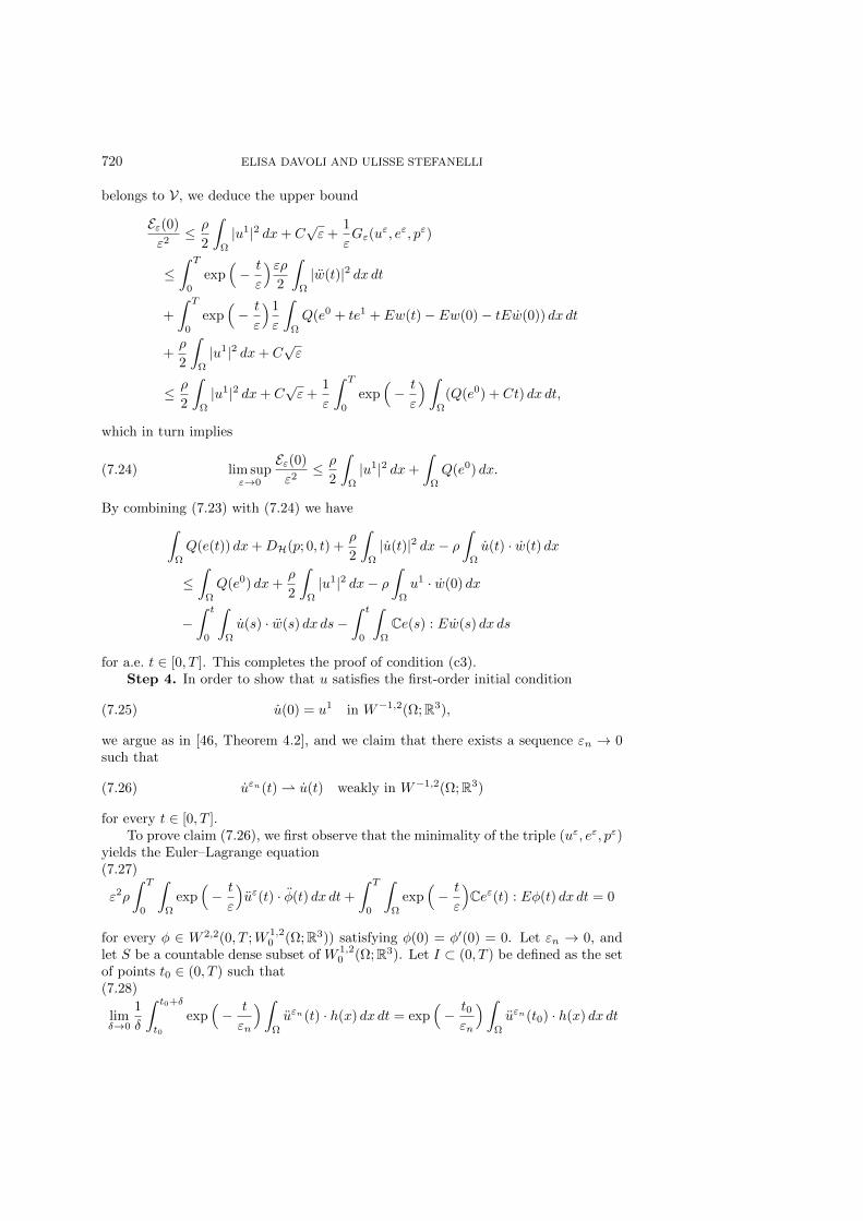
720 ELISA DAVOLI AND ULISSE STEFANELLI
belongs to \scrV , we deduce the upper bound
\scrE \varepsilon (0)\varepsilon 2
\leq \rho
2
\int
\Omega
| u1| 2 dx+ C\surd \varepsilon +
1
\varepsilon G\varepsilon (u
\varepsilon , e\varepsilon , p\varepsilon )
\leq \int T
0
exp\Bigl( - t
\varepsilon
\Bigr) \varepsilon \rho 2
\int
\Omega
| \"w(t)| 2 dx dt
+
\int T
0
exp\Bigl( - t
\varepsilon
\Bigr) 1\varepsilon
\int
\Omega
Q(e0 + te1 + Ew(t) - Ew(0) - tE \.w(0)) dx dt
+\rho
2
\int
\Omega
| u1| 2 dx+ C\surd \varepsilon
\leq \rho
2
\int
\Omega
| u1| 2 dx+ C\surd \varepsilon +
1
\varepsilon
\int T
0
exp\Bigl( - t
\varepsilon
\Bigr) \int
\Omega
(Q(e0) + Ct) dx dt,
which in turn implies
(7.24) lim sup\varepsilon \rightarrow 0
\scrE \varepsilon (0)\varepsilon 2
\leq \rho
2
\int
\Omega
| u1| 2 dx+
\int
\Omega
Q(e0) dx.
By combining (7.23) with (7.24) we have
\int
\Omega
Q(e(t)) dx+D\scrH (p; 0, t) +\rho
2
\int
\Omega
| \.u(t)| 2 dx - \rho
\int
\Omega
\.u(t) \cdot \.w(t) dx
\leq \int
\Omega
Q(e0) dx+\rho
2
\int
\Omega
| u1| 2 dx - \rho
\int
\Omega
u1 \cdot \.w(0) dx
- \int t
0
\int
\Omega
\.u(s) \cdot \"w(s) dx ds - \int t
0
\int
\Omega
\BbbC e(s) : E \.w(s) dx ds
for a.e. t \in [0, T ]. This completes the proof of condition (c3).Step 4. In order to show that u satisfies the first-order initial condition
(7.25) \.u(0) = u1 in W - 1,2(\Omega ;\BbbR 3),
we argue as in [46, Theorem 4.2], and we claim that there exists a sequence \varepsilon n \rightarrow 0such that
(7.26) \.u\varepsilon n(t)\rightharpoonup \.u(t) weakly in W - 1,2(\Omega ;\BbbR 3)
for every t \in [0, T ].To prove claim (7.26), we first observe that the minimality of the triple (u\varepsilon , e\varepsilon , p\varepsilon )
yields the Euler--Lagrange equation(7.27)
\varepsilon 2\rho
\int T
0
\int
\Omega
exp\Bigl( - t
\varepsilon
\Bigr) \"u\varepsilon (t) \cdot \"\phi (t) dx dt+
\int T
0
\int
\Omega
exp\Bigl( - t
\varepsilon
\Bigr) \BbbC e\varepsilon (t) : E\phi (t) dx dt = 0
for every \phi \in W 2,2(0, T ;W 1,20 (\Omega ;\BbbR 3)) satisfying \phi (0) = \phi \prime (0) = 0. Let \varepsilon n \rightarrow 0, and
let S be a countable dense subset of W 1,20 (\Omega ;\BbbR 3). Let I \subset (0, T ) be defined as the set
of points t0 \in (0, T ) such that(7.28)
lim\delta \rightarrow 0
1
\delta
\int t0+\delta
t0
exp\Bigl( - t
\varepsilon n
\Bigr) \int
\Omega
\"u\varepsilon n(t) \cdot h(x) dx dt = exp\Bigl( - t0\varepsilon n
\Bigr) \int
\Omega
\"u\varepsilon n(t0) \cdot h(x) dx dt

DYNAMIC PERFECT PLASTICITY AS CONVEX MINIMIZATION 721
for every n \in \BbbN and for every h \in S. Note that by the Lebesgue differentiationtheorem the set [0, T ] \setminus I is negligible.
Fix t0 \in I, and let \varphi \delta n \in C1,1(\BbbR ) be defined as
\varphi \delta n(t) :=
\left\
0 t \leq t0,
(t - t0)2
\delta \varepsilon 2nt \in (t0, t0 + \delta ),
2(t - t0)
\varepsilon 2n - \delta
\varepsilon 2nt \geq t0 + \delta .
We observe that
\varphi \prime \prime \delta n(t) =
2
\delta \varepsilon 2n\chi (t0,t0+\delta )(t),
where \chi (t0,t0+\delta ) is the characteristic function of (t0, t0 + \delta ). In addition,
| \varphi \delta n(t)| \leq 2
\varepsilon 2n(t - t0)
+ and \varphi \delta n(t) \rightarrow 2
\varepsilon 2n(t - t0)
+
as \delta \rightarrow 0 for almost every t \in (0, T ). Choosing \phi (t, x) = \varphi \delta n(t)h(x), with h \in S, by(7.27) we obtain
2\rho
\delta
\int t0+\delta
t0
\int
\Omega
exp\Bigl( - t
\varepsilon n
\Bigr) \"u\varepsilon n(t) \cdot h(x) dx dt
+
\int T
t0
\int
\Omega
exp\Bigl( - t
\varepsilon n
\Bigr) \varphi \delta n(t)\BbbC e\varepsilon n(t) : Eh(x) dx dt = 0.
Letting \delta \rightarrow 0, (7.28) and the dominated convergence theorem yield
\rho
\int
\Omega
\"u\varepsilon n(t0) \cdot h(x) dx+1
\varepsilon 2n
\int T
t0
\int
\Omega
exp\Bigl( t0 - t
\varepsilon n
\Bigr) (t - t0)\BbbC e\varepsilon n(t) : Eh(x) dx dt = 0.
By (5.42), there holds
\bigm| \bigm| \bigm| 1\varepsilon n
\int T
t0
\int
\Omega
exp\Bigl( t0 - t
\varepsilon n
\Bigr) (t - t0)\BbbC e\varepsilon n(t) : Eh(x) dx dt
\bigm| \bigm| \bigm|
\leq C
\varepsilon n\| e\varepsilon n\| L2(0,T ;L2(\Omega ;\BbbM 3\times 3
sym))\| Eh\| L2(\Omega ;\BbbM 3\times 3sym)
\Bigl( \int T
t0
exp\Bigl( 2(t0 - t)
\varepsilon n
\Bigr) (t - t0)
2 dt\Bigr) 1
2
\leq C\surd \varepsilon n\| h\| W 1,2
0 (\Omega ;\BbbR 3)
\Bigl( \int (T - t0)\varepsilon n
0
t2 exp( - 2t) dt\Bigr) 1
2 \leq C\| h\| W 1,20 (\Omega ;\BbbR 3),
where in the last inequality we used the fact that for t large there holds t2 exp( - 2t) \leq 1.
Thus,
\rho \bigm| \bigm| \bigm| \int
\Omega
\"u\varepsilon n(t0)h(x) dx\bigm| \bigm| \bigm| \leq C\| h\| W 1,2
0 (\Omega ;\BbbR 3),
where the constant C is independent of \varepsilon n and t0. In particular, we obtain the uniformestimate
(7.29) \rho \| \"u\varepsilon n\| L\infty (0,T ;W - 1,2(\Omega ;\BbbR 3)) \leq C.

722 ELISA DAVOLI AND ULISSE STEFANELLI
By combining (5.42), (7.3), and (7.29), we deduce that
\| \.u\varepsilon n\| W 1,2(0,T ;W - 1,2(\Omega ;\BbbR 3)) \leq C.
In particular, as W 1,2(0, T ;W - 1,2(\Omega ;\BbbR 3)) embeds into Cw([0, T ];W - 1,2(\Omega ;\BbbR 3)), up
to the extraction of a (non--relabeled) subsequence we obtain claim (7.26), which inturn yields \.u(0) = u1.
As pointed out in [36, Remark 3.2], arguing as in [7] one obtains that (c3) holdswith an equality. The additional regularity in time of the solution follows by adaptingthe argument in [36, Proof of Theorem 3.1]. The thesis follows now by the uniquenessof solutions for the dynamic plasticity problem (see Theorem 2.2).
We point out that the assertion of Theorem 2.3 still holds if we generalize theminimum problem (2.14) by imposing \varepsilon -dependent initial data satisfying suitablecompatibility assumptions. To be precise, for every \varepsilon , define the set
\scrV \varepsilon := \ (u, e, p) \in W 2,2(0, T ;L2(\Omega ;\BbbR 3)) \cap L1(0, T ;BD(\Omega ))
\times L2((0, T )\times \Omega ;\BbbM 3\times 3sym)\times BV ([0, T ];\scrM b(\Omega \cup \Gamma 0;\BbbM 3\times 3
D )) :
(u(t), e(t), p(t)) \in A (w(t)) for a.e. t \in [0, T ],
Eu(t) = e(t) + p(t) in \scrD \prime (\Omega ;\BbbM 3\times 3sym) for every t \in [0, T ],
u(0) = u0\varepsilon , \.u(0) = u1\varepsilon , e(0) = e0\varepsilon , p(0) = p0\varepsilon \ ,
with (u0\varepsilon , e0\varepsilon , p
0\varepsilon ) \in A (w(0)), and u1\varepsilon \in W 1,2(\Omega ;\BbbR 3) such that u1\varepsilon = \.w(0) on \Gamma 0.
Assuming that the initial data are well prepared, namely,
u0\varepsilon \rightharpoonup \ast u0 weakly* in BD(\Omega ),
e0\varepsilon \rightharpoonup e0 weakly in L2(\Omega ;\BbbM 3\times 3sym),
p0\varepsilon \rightharpoonup \ast p0 weakly* in \scrM b(\Omega \cup \Gamma 0;\BbbM 3\times 3
D ),
u1\varepsilon \rightarrow u1 strongly in W - 1,2(\Omega ;\BbbR 3),
and
lim\varepsilon \rightarrow 0
\Bigl[ \int
\Omega
Q(e0\varepsilon ) dx+\rho
2
\int
\Omega
| u1\varepsilon | 2 dx - \rho
\int
\Omega
u1\varepsilon \cdot \.w(0) dx\Bigr]
=
\int
\Omega
Q(e0) dx+\rho
2
\int
\Omega
| u1| 2 dx - \rho
\int
\Omega
u1 \cdot \.w(0) dx,
one can again prove there exists a sequence of triples \ (u\varepsilon , e\varepsilon , p\varepsilon )\ , with (u\varepsilon , e\varepsilon , p\varepsilon ) \subset \scrV \varepsilon for every \varepsilon such that
I\varepsilon (u\varepsilon , e\varepsilon , p\varepsilon ) = min
(v,f,q)\in \scrV \varepsilon
I\varepsilon (v, f, q),
such that \ (u\varepsilon , e\varepsilon , p\varepsilon )\ converges to the solution (u, e, p) of dynamic perfect plasticity,namely (c1), (c2), and (c3), in the sense of Theorem 2.3.
Appendix A. This appendix is devoted to the proof of Proposition 6.7. Westart with a somewhat technical lemma.
Lemma A.1. Let \mu \in BV (0, T ;\scrM b(\Omega \cup \Gamma 0;\BbbM 3\times 3D )), and let \varphi \in C\infty
c (0, T ). Then,
\^D\scrH (\varphi ;\mu ; 0, T ) = - \int T
0
\.\varphi (t)D\scrH (\mu ; 0, t) dt.

DYNAMIC PERFECT PLASTICITY AS CONVEX MINIMIZATION 723
Proof. In view of [21, Theorem 4.5], there holds (see also [21, Theorem 2.15])
\^D\scrH (\varphi ;\mu ; 0, T ) = - PMS
\int T
0
D\scrH (\mu ; 0, t) d\varphi
= - RS\int T
0
D\scrH (\mu ; 0, t) d\varphi = - \int T
0
D\scrH (\mu ; 0, t) \.\varphi (t) dt,
where PMS\int andRS
\int denote the Pollard--Moore--Stieltjes and the Riemann--Stieltjes
integrals, respectively (see [21, section 4]), and where the last equality is due to theregularity of \varphi and to classical properties of the Riemann--Stieltjes integral.
We are now in a position to prove Proposition 6.7.
Proof of Proposition 6.7. We argue as in [38, Proposition 4.1] by comparing theenergy associated to (u\varepsilon , e\varepsilon , p\varepsilon ) with that of a rescaled triple (\~u\varepsilon , \~e\varepsilon , \~p\varepsilon ). Consider anincreasing diffeomorphism
\beta \delta : [0, T ] \rightarrow [0, T ]
such that \beta \delta \in C2([0, T ]), \beta \delta (0) = 0, \beta \delta (T ) = T , and \.\beta \delta (0) = 1. We set
\~u\varepsilon (s) := u\varepsilon (\beta - 1\delta (s)) - w(\beta - 1
\delta (s)) + w(s), \~p\varepsilon (s) := p\varepsilon (\beta - 1\delta (s)),
for every s \in [0, T ], and
\~e\varepsilon (s) := e\varepsilon (\beta - 1\delta (s)) - Ew(\beta - 1
\delta (s)) + Ew(s)
for every s \in [0, T ]. It is easy to check that (\~u\varepsilon , \~e\varepsilon , \~p\varepsilon ) \in \scrV . Hence, by the minimalityof (u\varepsilon , e\varepsilon , p\varepsilon ) there holds
(A.1) G\varepsilon (\~u\varepsilon , \~e\varepsilon , \~p\varepsilon ) - G\varepsilon (u
\varepsilon , e\varepsilon , p\varepsilon ) \geq 0.
Using the definition of (\~u\varepsilon , \~e\varepsilon , \~p\varepsilon ), we can rewrite its associated energy as
G\varepsilon (\~u\varepsilon , \~e\varepsilon , \~p\varepsilon ) =
\int T
0
exp\Bigl( - \beta \delta (t)
\varepsilon
\Bigr) \.\beta \delta (t)
\int
\Omega
Q\bigl( e\varepsilon (t) - Ew(t) + Ew(\beta \delta (t))
\bigr) dx dt
+\varepsilon 2\rho
2
\int T
0
exp\Bigl( - \beta \delta (t)
\varepsilon
\Bigr) \.\beta \delta (t)
\Bigl( \int
\Omega
\bigm| \bigm| \bigm| \"u\varepsilon (t)
( \.\beta \delta (t))2 - \.u\varepsilon (t) \"\beta \delta (t)
( \.\beta \delta (t))3 - \"w(t)
( \.\beta \delta (t))2
+\.w(t) \"\beta \delta (t)
( \.\beta \delta (t))3+ \"w(\beta \delta (t))
\bigm| \bigm| \bigm| 2
dx\Bigr) dt+ \varepsilon D\scrH (exp( - \cdot /\varepsilon ); \~p\varepsilon ; 0, T ).
Along the lines of [38, Proposition 4.1], we fix \varphi \in C\infty c (0, T ). Let \delta \in (0, 1) be such
that \varepsilon \delta \.\varphi (t) < exp( - t/\varepsilon ) for every t \in [0, T ], and define \beta \delta as the solution to
(A.2) exp\Bigl( - \beta \delta (t)
\varepsilon
\Bigr) - exp
\Bigl( - t
\varepsilon
\Bigr) = \delta \varphi (t).
We immediately see that \beta \delta (0) = 0 and \beta \delta (T ) = T . In addition, deriving (A.2) withrespect to time, we have
(A.3) \.\beta \delta (t) = exp\Bigl( \beta \delta (t)
\varepsilon
\Bigr) \Bigl( exp
\Bigl( - t
\varepsilon
\Bigr) - \varepsilon \delta \.\varphi (t)
\Bigr)
for every t \in [0, T ], yielding \.\beta \delta (t) > 0 for every t \in (0, T ) and \.\beta \delta (0) = 1. As alreadyobserved in [38, Proposition 4.1],
(A.4) \beta \delta (t) = t - \varepsilon \delta \varphi (t) exp\Bigl( t\varepsilon
\Bigr) +O(\delta 2).

724 ELISA DAVOLI AND ULISSE STEFANELLI
In addition, by (A.2) and (A.3),
(A.5) \.\beta \delta (t) = 1 - \delta (\varphi (t) + \varepsilon \.\varphi (t)) exp\Bigl( t\varepsilon
\Bigr) +O(\delta 2),
and by performing a further derivation in time of (A.3),
(A.6) \"\beta \delta (t) = - \delta \Bigl( \varphi (t)
\varepsilon + 2 \.\varphi (t) + \varepsilon \"\varphi (t)
\Bigr) exp
\Bigl( t\varepsilon
\Bigr) +O(\delta 2).
Let us first observe that
lim\delta \rightarrow 0
1
\delta
\Bigl\ \int T
0
exp\Bigl( - \beta \delta (t)
\varepsilon
\Bigr) \.\beta \delta (t)
\int
\Omega
Q\bigl( e\varepsilon (t) - Ew(t) + Ew(\beta \delta (t))
\bigr) dx dt(A.7)
- \int T
0
exp\Bigl( - t
\varepsilon
\Bigr) \int
\Omega
Q\bigl( e\varepsilon (t)
\bigr) dx dt
\Bigr\
= lim\delta \rightarrow 0
1
\delta
\Bigl\ \int T
0
\Bigl( exp
\Bigl( - \beta \delta (t)
\varepsilon
\Bigr) \.\beta \delta (t) - exp
\Bigl( - t
\varepsilon
\Bigr) \Bigr) \int
\Omega
Q\bigl( e\varepsilon (t)
\bigr) dx dt
+
\int T
0
exp\Bigl( - \beta \delta (t)
\varepsilon
\Bigr) \.\beta \delta (t)
\int
\Omega
Q\bigl( Ew(t) - Ew(\beta \delta (t))
\bigr) dx dt
- \int T
0
exp\Bigl( - \beta \delta (t)
\varepsilon
\Bigr) \.\beta \delta (t)
\int
\Omega
\BbbC e\varepsilon (t) :\Bigl( Ew(t) - Ew(\beta \delta (t))
\Bigr) dx dt
\Bigr\ .
In view of (A.2) and (A.5), and by the dominated convergence theorem, the first termin the right-hand side of (A.7) becomes
lim\delta \rightarrow 0
1
\delta
\int T
0
\Bigl( exp
\Bigl( - \beta \delta (t)
\varepsilon
\Bigr) \.\beta \delta (t) - exp
\Bigl( - t
\varepsilon
\Bigr) \Bigr) \int
\Omega
Q\bigl( e\varepsilon (t)
\bigr) dx dt(A.8)
= lim\delta \rightarrow 0
1
\delta
\int T
0
\Bigl( \Bigl( \delta \varphi (t) + exp
\Bigl( - t
\varepsilon
\Bigr) \Bigr) \.\beta \delta (t) - exp
\Bigl( - t
\varepsilon
\Bigr) \Bigr) \int
\Omega
Q\bigl( e\varepsilon (t)
\bigr) dx dt
= - \varepsilon \int T
0
\.\varphi (t)
\int
\Omega
Q\bigl( e\varepsilon (t)
\bigr) dx dt.
By the regularity of w and by (A.4) there holds
| Ew(t) - Ew(\beta \delta (t))| =\bigm| \bigm| \bigm| \int \beta \delta (t)
t
E \.w(\xi ) d\xi \bigm| \bigm| \bigm| \leq
\surd \delta \| w\| W 1,2(0,T ;W 1,2(\Omega ;\BbbR 3)).
Hence, by (A.2) and (A.5) one obtains
lim\delta \rightarrow 0
1
\delta
\int T
0
exp\Bigl( - \beta \delta (t)
\varepsilon
\Bigr) \.\beta \delta (t)
\int
\Omega
Q\bigl( Ew(t) - Ew(\beta \delta (t))
\bigr) dx dt = 0.(A.9)

DYNAMIC PERFECT PLASTICITY AS CONVEX MINIMIZATION 725
Finally, by (A.2), (A.5), and the mean value theorem we get
lim\delta \rightarrow 0
1
\delta
\int T
0
exp\Bigl( - \beta \delta (t)
\varepsilon
\Bigr) \.\beta \delta (t)
\int
\Omega
\BbbC e\varepsilon (t) :\Bigl( Ew(t) - Ew(\beta \delta (t))
\Bigr) dx dt
(A.10)
= lim\delta \rightarrow 0
1
\delta
\int T
0
\Bigl( exp
\Bigl( - t
\varepsilon
\Bigr) + \delta \varepsilon \.\varphi (t)
\Bigr) \int
\Omega
\BbbC e\varepsilon (t) :\Bigl( \int \beta \delta (t)
t
E \.w(\xi ) d\xi \Bigr) dx dt
= lim\delta \rightarrow 0
1
\delta
\int T
0
\Bigl( exp
\Bigl( - t
\varepsilon
\Bigr) + \delta \varepsilon \.\varphi (t)
\Bigr) \int \beta \delta (t)
t
\int
\Omega
\BbbC e\varepsilon (t) : E \.w(\xi ) dx d\xi dt
= - \varepsilon lim\delta \rightarrow 0
\int T
0
\varphi (t)
\int
\Omega
\BbbC e\varepsilon (t) : E \.w(\xi t) dx dt = - \varepsilon \int T
0
\varphi (t)
\int
\Omega
\BbbC e\varepsilon (t) : E \.w(t) dx dt,
where, in the second-to-last line, for every t \in [0, T ], \xi t is an intermediate valuebetween t and \beta \delta (t). By combining (A.7)--(A.10) we obtain
lim\delta \rightarrow 0
1
\delta
\Bigl\ \int T
0
exp\Bigl( - \beta \delta (t)
\varepsilon
\Bigr) \.\beta \delta (t)
\int
\Omega
Q\bigl( e\varepsilon (\beta \delta (t)) - Ew(t) + Ew(\beta \delta (t))
\bigr) dx dt(A.11)
- \int T
0
exp\Bigl( - t
\varepsilon
\Bigr) \int
\Omega
Q\bigl( e\varepsilon (t)
\bigr) dx dt
\Bigr\
= - \varepsilon \int T
0
\.\varphi (t)
\int
\Omega
Q\bigl( e\varepsilon (t)
\bigr) dx dt+ \varepsilon
\int T
0
\varphi (t)
\int
\Omega
\BbbC e\varepsilon (t) : E \.w(t) dx dt.
We proceed by performing the analogous computation for the inertial term. Weseek to estimate
lim\delta \rightarrow 0
1
\delta
\Bigl\ \varepsilon 2\rho 2
\int T
0
exp\Bigl( - \beta \delta (t)
\varepsilon
\Bigr) \.\beta \delta (t)
\Bigl( \int
\Omega
\bigm| \bigm| \bigm| \"u\varepsilon (t)
( \.\beta \delta (t))2 - \.u\varepsilon (t) \"\beta \delta (t)
( \.\beta \delta (t))3 - \"w(t)
( \.\beta \delta (t))2
(A.12)
+\.w(t) \"\beta \delta (t)
( \.\beta \delta (t))3+ \"w(\beta \delta (t))
\bigm| \bigm| \bigm| 2
dx\Bigr) dt - \varepsilon 2\rho
2
\int T
0
exp\Bigl( - t
\varepsilon
\Bigr) \int
\Omega
| \"u\varepsilon (t)| 2 dx dt\Bigr\ .
By (A.2) and (A.5) we have
lim\delta \rightarrow 0
1
\delta
\varepsilon 2\rho
2
\int T
0
\Bigl( 1
( \.\beta \delta (t))3exp
\Bigl( - \beta \delta (t)
\varepsilon
\Bigr) - exp
\Bigl( - t
\varepsilon
\Bigr) \Bigr) \int
\Omega
| \"u\varepsilon (t)| 2 dx dt(A.13)
=3\varepsilon 3\rho
2
\int T
0
\.\varphi (t)
\int
\Omega
| \"u\varepsilon (t)| 2 dx dt+ 2\varepsilon 2\rho
\int T
0
\varphi (t)
\int
\Omega
| \"u\varepsilon (t)| 2 dx dt.
By (A.2), (A.5), and (A.6) there holds
lim\delta \rightarrow 0
1
\delta
\varepsilon 2\rho
2
\int T
0
exp\Bigl( - \beta \delta (t)
\varepsilon
\Bigr) \int
\Omega
\Bigl[ ( \"\beta \delta (t))2( \.\beta \delta (t))5
(| \.u\varepsilon (t)| 2 + | \.w(t)| 2 - 2 \.u\varepsilon (t) \cdot \.w(t))\Bigr] dx dt = 0,
(A.14)

726 ELISA DAVOLI AND ULISSE STEFANELLI
as well as
lim\delta \rightarrow 0
1
\delta \varepsilon 2\rho
\int T
0
exp\Bigl( - \beta \delta (t)
\varepsilon
\Bigr) \int
\Omega
\"\beta \delta (t)
( \.\beta \delta (t))4\"u\varepsilon (t) \cdot ( \.w(t) - \.u\varepsilon (t)) dx dt(A.15)
= - \varepsilon 3\rho \int T
0
\"\varphi (t)\"u\varepsilon (t) \cdot ( \.w(t)
- \.u\varepsilon (t)) dx dt - \varepsilon \rho
\int T
0
(\varphi (t) + 2\varepsilon \.\varphi (t))\"u\varepsilon (t) \cdot ( \.w(t) - \.u\varepsilon (t)) dx dt.
To estimate the remaining term, we observe that by (A.5) and in view of the regularityof the boundary datum,
- \"w(t)
( \.\beta \delta (t))2+ \"w(\beta \delta (t)) = - \"w(t)
( \.\beta \delta (t))2(1 - ( \.\beta \delta (t))
2) +
\int \beta \delta (t)
t
...w(\xi ) d\xi
= - 2\delta \"w(t)
( \.\beta \delta (t))2(\varphi (t) + \varepsilon \.\varphi (t)) exp
\Bigl( t\varepsilon
\Bigr) +
\int \beta \delta (t)
t
...w(\xi ) d\xi +O(\delta 2).
By the regularity of w, by (A.4), and by Lebesgue's theorem,
lim\delta \rightarrow 0
\bigm\| \bigm\| \bigm\| 1\delta
\int \beta \delta (t)
t
...w(\xi ) d\xi + \varepsilon
...w(t)\varphi (t) exp
\Bigl( t\varepsilon
\Bigr) \bigm\| \bigm\| \bigm\| 2
L2(0,T ;L2(\Omega ;\BbbR 3))
= lim\delta \rightarrow 0
\bigm\| \bigm\| \bigm\| 1\delta
\int \beta \delta (t)
t
(...w(\xi ) - ...
w(t)) d\xi \bigm\| \bigm\| \bigm\| 2
L2(0,T ;L2(\Omega ;\BbbR 3))
\leq lim\delta \rightarrow 0
1
\delta
\int T
0
\int t+\delta \varepsilon \| \varphi \| L\infty (0,T ) exp(T/\varepsilon )
t - \delta \varepsilon \| \varphi \| L\infty (0,T ) exp(T/\varepsilon )
\int
\Omega
| ...w(\xi ) - ...w(t)| 2 dx d\xi dt = 0.
Therefore, by (A.5) and (A.6),
lim\delta \rightarrow 0
1
\delta
\Bigl\ \varepsilon 2\rho 2
\int T
0
exp\Bigl( - \beta \delta (t)
\varepsilon
\Bigr) \.\beta \delta (t)
\int
\Omega
\Bigl[ \bigm| \bigm| \bigm| - \"w(t)
( \.\beta \delta (t))2+ \"w(\beta \delta (t))
\bigm| \bigm| \bigm| 2
(A.16)
+ 2\Bigl( - \"w(t)
( \.\beta \delta (t))2+ \"w(\beta \delta (t))
\Bigr) \cdot ( \.w(t) - \.u\varepsilon (t)) \"\beta \delta (t)
( \.\beta \delta (t))3
\Bigr] dx dt
\Bigr\ = 0,
and
lim\delta \rightarrow 0
1
\delta \varepsilon 2\rho
\int T
0
exp\Bigl( - \beta \delta (t)
\varepsilon
\Bigr) \.\beta \delta (t)
\int
\Omega
\"u\varepsilon (t)
( \.\beta \delta (t))2\cdot \Bigl( - \"w(t)
( \.\beta \delta (t))2+ \"w(\beta \delta (t))
\Bigr) dx dt
(A.17)
= - 2\varepsilon 2\rho
\int T
0
\int
\Omega
\"u\varepsilon (t) \cdot \"w(t)(\varphi (t) + \varepsilon \.\varphi (t)) dx dt
- \varepsilon 3\rho
\int T
0
\int
\Omega
\"u\varepsilon (t) \cdot ...w(t)\varphi (t) dx dt.

DYNAMIC PERFECT PLASTICITY AS CONVEX MINIMIZATION 727
By combining (A.12)--(A.17), we obtain
lim\delta \rightarrow 0
1
\delta
\Bigl\ \varepsilon 2\rho 2
\int T
0
exp\Bigl( - \beta \delta (t)
\varepsilon
\Bigr) \.\beta \delta (t)
\int
\Omega
\bigm| \bigm| \bigm| \"u\varepsilon (t)
( \.\beta \delta (t))2 - \.u\varepsilon (t) \"\beta \delta (t)
( \.\beta \delta (t))3 - \"w(t)
( \.\beta \delta (t))2(A.18)
+\.w(t) \"\beta \delta (t)
( \.\beta \delta (t))3+ \"w(\beta \delta (t))
\bigm| \bigm| \bigm| 2
dx dt - \varepsilon 2\rho
2
\int T
0
exp\Bigl( - t
\varepsilon
\Bigr) \int
\Omega
| \"u\varepsilon (t)| 2 dx dt\Bigr\
=3\varepsilon 3\rho
2
\int T
0
\.\varphi (t)
\int
\Omega
| \"u\varepsilon (t)| 2 dx dt+ 2\varepsilon 2\rho
\int T
0
\varphi (t)
\int
\Omega
| \"u\varepsilon (t)| 2 dx dt
- \varepsilon 3\rho
\int T
0
\int
\Omega
\"\varphi (t)\"u\varepsilon (t) \cdot ( \.w(t) - \.u\varepsilon (t)) dx dt
- \varepsilon \rho
\int T
0
\int
\Omega
(\varphi (t) + 2\varepsilon \.\varphi (t))\"u\varepsilon (t) \cdot ( \.w(t) - \.u\varepsilon (t)) dx dt
- 2\varepsilon 2\rho
\int T
0
\int
\Omega
\"u\varepsilon (t) \cdot \"w(t)(\varphi (t) + \varepsilon \.\varphi (t)) dx dt
- \varepsilon 3\rho
\int T
0
\int
\Omega
\"u\varepsilon (t) \cdot ...w(t)\varphi (t) dx dt.
To complete the proof of the \varepsilon -energy inequality it remains to estimate from abovethe quantity
(A.19) lim sup\delta \rightarrow 0
1
\delta
\bigl( D\scrH (exp( - \cdot /\varepsilon ); \~p\varepsilon ; 0, T ) - D\scrH (exp( - \cdot /\varepsilon ); p\varepsilon ; 0, T )
\bigr) .
To this end, fix \lambda > 0, and let 0 \leq t0 < t1 < \cdot \cdot \cdot < tm \leq T be such that
D\scrH (exp( - \cdot /\varepsilon ); \~p\varepsilon ; 0, T ) \leq m\sum
i=1
exp
\biggl( - ti\varepsilon
\biggr) \scrH (\~p\varepsilon (ti) - \~p\varepsilon (ri - 1)) + \lambda .
For i = 0, . . . ,m, let si \in [0, T ] be such that \beta \delta (si) = ti. By the properties of \beta \delta , itfollows that 0 \leq s0 < s1 < \cdot \cdot \cdot < sn \leq T . In view of (A.2), we have
m\sum
i=1
exp
\biggl( - ti\varepsilon
\biggr) \scrH (\~p\varepsilon (ti) - \~p\varepsilon (ri - 1)) =
m\sum
i=1
exp
\biggl( - \beta \delta (si)
\varepsilon
\biggr) \scrH (p\varepsilon (si) - p\varepsilon (si - 1))
=m\sum
i=1
exp\Bigl( - si\varepsilon
\Bigr) \scrH (p\varepsilon (si) - p\varepsilon (si - 1))
+m\sum
i=1
\Bigl( exp
\biggl( - \beta \delta (si)
\varepsilon
\biggr) - exp
\Bigl( - si\varepsilon
\Bigr) \Bigr) \scrH (p\varepsilon (si) - p\varepsilon (si - 1))
\leq D\scrH (exp( - \cdot /\varepsilon ); p\varepsilon ; 0, T ) + \delta m\sum
i=1
\varphi (si)\scrH (p\varepsilon (si) - p\varepsilon (si - 1)).
By considering finer and finer refinements of \ t0, . . . , tm\ , in view of the definitionof \^D\scrH , and by the arbitrariness of \lambda we conclude that
D\scrH (exp( - \cdot /\varepsilon ); \~p\varepsilon ; 0, T ) \leq D\scrH (exp( - \cdot /\varepsilon ); p\varepsilon ; 0, T ) + \delta \^D\scrH (\varphi ; p\varepsilon ; 0, T ).
Thus, we can bound (A.19) from above as(A.20)
lim sup\delta \rightarrow 0
1
\delta
\bigl( D\scrH (exp( - \cdot /\varepsilon ); \~p\varepsilon ; 0, T ) - D\scrH (exp( - \cdot /\varepsilon ); p\varepsilon ; 0, T )
\bigr) \leq \^D\scrH (\varphi ; p\varepsilon ; 0, T ),

728 ELISA DAVOLI AND ULISSE STEFANELLI
where \^D\scrH is the quantity defined in (2.8). Combining (A.1), (A.11), (A.18), (A.20),and Lemma A.1 we finally obtain the inequality
0 \leq lim sup\delta \rightarrow 0
1
\varepsilon \delta (G\varepsilon (\~u
\varepsilon , \~e\varepsilon , \~p\varepsilon ) - G(u\varepsilon , e\varepsilon , p\varepsilon ))(A.21)
\leq - \int T
0
\.\varphi (t)
\int
\Omega
Q\bigl( e\varepsilon (t)
\bigr) dx dt -
\int T
0
\varphi (t)
\int
\Omega
\BbbC e\varepsilon (t) : E \.w(t) dx dt
+3\varepsilon 2\rho
2
\int T
0
\.\varphi (t)
\int
\Omega
| \"u\varepsilon (t)| 2 dx dt+ 2\varepsilon \rho
\int T
0
\varphi (t)
\int
\Omega
| \"u\varepsilon (t)| 2 dx dt
- \varepsilon 2\rho
\int T
0
\int
\Omega
\"\varphi (t)\"u\varepsilon (t) \cdot ( \.w(t) - \.u\varepsilon (t)) dx dt
- \rho
\int T
0
\int
\Omega
(\varphi (t) + 2\varepsilon \.\varphi (t))\"u\varepsilon (t) \cdot ( \.w(t) - \.u\varepsilon (t)) dx dt
- 2\varepsilon \rho
\int T
0
\int
\Omega
\"u\varepsilon (t) \cdot \"w(t)(\varphi (t) + \varepsilon \.\varphi (t)) dx dt
- \varepsilon 2\rho
\int T
0
\int
\Omega
\"u\varepsilon (t) \cdot ...w(t)\varphi (t) dx dt
- \int T
0
D\scrH (p\varepsilon ; 0, t) \.\varphi (t) dt
for every \varphi \in C\infty c (0, T ). The weak energy equality (6.18) follows now by performing
an integration by parts.
Acknowledgment. The careful reading by the anonymous referees is gratefullyacknowledged.
REFERENCES
[1] G. Akagi and U. Stefanelli, A variational principle for doubly nonlinear evolution, Appl.Math. Lett., 23 (2010), pp. 1120--1124.
[2] G. Akagi and U. Stefanelli, Periodic solutions for doubly nonlinear evolution equations, J.Differential Equations, 251 (2011), pp. 1790--1812.
[3] G. Akagi and U. Stefanelli, Weighted energy-dissipation functionals for doubly nonlinearevolution, J. Funct. Anal., 260 (2011), pp. 2541--2578.
[4] G. Akagi and U. Stefanelli, Doubly nonlinear equations as convex minimization, SIAM J.Math. Anal., 46 (2014), pp. 1922--1945, https://doi.org/10.1137/13091909X.
[5] G. Akagi, S. Melchionna, and U. Stefanelli, Weighted energy-dissipation approach todoubly-nonlinear problems on the half line, J. Evol. Equ., 18 (2018), pp. 49--74.
[6] G. Anzellotti and S. Luckhaus, Dynamical evolution of elasto-perfectly plastic bodies, Appl.Math. Optim., 15 (1987), pp. 121--140.
[7] J.-F. Babadjian and M. G. Mora, Approximation of dynamic and quasi-static evolutionproblems in plasticity by cap models, Quart. Appl. Math., 73 (2015), pp. 265--316.
[8] V. B\"ogelein, F. Duzaar, and P. Marcellini, Existence of evolutionary variational solutionsvia the calculus of variations, J. Differential Equations, 256 (2014), pp. 3912--3942.
[9] H. Brezis, Functional Analysis, Sobolev Spaces and Partial Differential Equations, Springer,New York, 2011.
[10] S. Conti and M. Ortiz, Minimum principles for the trajectories of systems governed by rateproblems, J. Mech. Phys. Solids, 56 (2008), pp. 1885--1904.
[11] G. Dal Maso, A. DeSimone, and M. G. Mora, Quasistatic evolution problems for linearlyelastic-perfectly plastic materials, Arch. Ration. Mech. Anal., 180 (2006), pp. 237--291.
[12] G. Dal Maso and R. Scala, Quasistatic evolution in perfect plasticity as limit of dynamicprocesses, J. Dynam. Differential Equations, 26 (2014), pp. 915--954.
[13] E. Davoli and M. G. Mora, A quasistatic evolution model for perfectly plastic plates derivedby \Gamma -convergence, Ann. Inst. H. Poincar\'e Anal. Non Lin\'eaire, 30 (2013), pp. 615--660.

DYNAMIC PERFECT PLASTICITY AS CONVEX MINIMIZATION 729
[14] E. De Giorgi, Conjectures concerning some evolution problems, Duke Math. J., 81 (1996), pp.255--268.
[15] E. De Giorgi and T. Franzoni, On a type of variational convergence, in Proceedings of theBrescia Mathematical Seminar, Vol. 3, Univ. Cattolica Sacro Cuore., Milan, 1979, pp.63--101 (in Italian).
[16] G. Duvaut and J.-L. Lions, Inequalities in Mechanics and Physics, Grundlehren Math. Wiss.219, Springer-Verlag, New York, 1976.
[17] L. C. Evans, Partial Differential Equations, Grad. Stud. Math. 19, American MathematicalSociety, Providence, RI, 1998.
[18] G. A. Francfort and A. Giacomini, On periodic homogenization in perfect plasticity, J. Eur.Math. Soc. (JEMS), 16 (2014), pp. 409--461.
[19] C. Goffman and J. Serrin, Sublinear functions of measures and variational integrals, DukeMath. J., 31 (1964), pp. 159--178.
[20] W. Han and B. D. Reddy, Plasticity, Mathematical Theory and Numerical Analysis, Springer-Verlag, New York, 1999.
[21] T. H. Hildebrandt, Definitions of Stieltjes integrals of the Riemann type, Amer. Math.Monthly, 45 (1938), pp. 265--278.
[22] R. Hill, The Mathematical Theory of Plasticity, Clarendon Press, Oxford, 1950.[23] N. Hirano, Existence of periodic solutions for nonlinear evolution equations in Hilbert spaces,
Proc. Amer. Math. Soc., 120 (1994), pp. 185--192.[24] T. Ilmanen, Elliptic regularization and partial regularity for motion by mean curvature, Mem.
Amer. Math. Soc., 108 (1994), no. 520.[25] R. Kohn and R. Temam, Dual spaces of stresses and strains, with applications to Hencky
plasticity, Appl. Math. Optim., 10 (1983), pp. 1--35.[26] C. J. Larsen, M. Ortiz, and C. L. Richardson, Fracture paths from front kinetics: Relax-
ation and rate independence, Arch. Ration. Mech. Anal., 193 (2009), pp. 539--583.[27] J. Lemaitre and J.-L. Chaboche, Mechanics of Solid Materials, Cambridge University Press,
Cambridge, 1990.[28] M. Liero and A. Mielke, An evolutionary elastoplastic plate model derived via \Gamma -convergence,
Math. Models Methods Appl. Sci., 21 (2011), pp. 1961--1986.[29] M. Liero and T. Roche, Rigorous derivation of a plate theory in linear elastoplasticity via
\Gamma -convergence, NoDEA Nonlinear Differential Equations Appl., 19 (2012), pp. 437--457.[30] M. Liero and U. Stefanelli, A new minimum principle for Lagrangian mechanics, J. Non-
linear Sci., 23 (2013), pp. 179--204.[31] M. Liero and U. Stefanelli, Weighted inertia-dissipation-energy functionals for semilinear
equations, Boll. Unione Mat. Ital. (9), 6 (2013), pp. 1--27.[32] J.-L. Lions, Singular Perturbations and Some Non Linear Boundary Value Problems, Technical
report 421, Mathematics Research Center, University of Wisconsin--Madison, Madison, WI,1963.
[33] J.-L. Lions, Sur certaines \'equations paraboliques non lin\'eaires, Bull. Soc. Math. France, 93(1965), pp. 155--175.
[34] J. Lubliner, Plasticity Theory, Macmillan, New York, 1990.[35] S. Luckhaus, Elastisch-plastische Materialien mit Viskosit\"at, preprint 65, Collaborative Re-
search Center 123, Heidelberg University, Heidelberg, 1980.[36] G. B. Maggiani and M. G. Mora, A dynamic evolution model for perfectly plastic plates,
Math. Models Methods Appl. Sci., 26 (2016), pp. 1825--1864.[37] S. Melchionna, A variational principle for nonpotential perturbations of gradient flows of
nonconvex energies, J. Differential Equations, 262 (2016), pp. 3737--3758.[38] A. Mielke and M. Ortiz, A class of minimum principles for characterizing the trajectories
and the relaxation of dissipative systems, ESAIM Control Optim. Calc. Var., 14 (2008),pp. 494--516.
[39] A. Mielke and T. Roub\'\i\v cek, Rate-Independent Systems, Appl. Math. Sci. 193, Springer, NewYork, 2015.
[40] A. Mielke and U. Stefanelli, A discrete variational principle for rate-independent evolution,Adv. Calc. Var., 1 (2008), pp. 399--431.
[41] A. Mielke and U. Stefanelli, Weighted energy-dissipation functionals for gradient flows,ESAIM Control Optim. Calc. Var., 17 (2011), pp. 52--85.
[42] M. G. Mora, Relaxation of the Hencky model in perfect plasticity, J. Math. Pures Appl., 106(2016), pp. 725--743.
[43] O. A. Ole\u inik, On a problem of G. Fichera, Dokl. Akad. Nauk SSSR, 157 (1964), pp. 1297--1300(in Russian).

730 ELISA DAVOLI AND ULISSE STEFANELLI
[44] R. Rossi, G. Savar\'e, A. Segatti, and U. Stefanelli, A variational principle for gradientflows in metric spaces, C. R. Math. Acad. Sci. Paris, 349 (2011), pp. 1225--1228.
[45] A. Segatti, A variational approach to gradient flows in metric spaces, Boll. Unione Mat. Ital.(9), 6 (2013), pp. 765--780.
[46] E. Serra and P. Tilli, Nonlinear wave equations as limits of convex minimization problems:Proof of a conjecture by De Giorgi, Ann. of Math. (2), 175 (2012), pp. 1551--1574.
[47] E. Serra and P. Tilli, A minimization approach to hyperbolic Cauchy problems, J. Eur. Math.Soc. (JEMS), 18 (2016), pp. 2019--2044.
[48] E. Spadaro and U. Stefanelli, A variational view at the time-dependent minimal surfaceequation, J. Evol. Equ., 11 (2011), pp. 793--809.
[49] U. Stefanelli, The De Giorgi conjecture on elliptic regularization, Math. Models MethodsAppl. Sci., 21 (2011), pp. 1377--1394.
[50] P. Suquet, Plasticit\'e et homog\'en\'eisation, Ph.D. thesis, Universit\'e Pierre et Marie Curie, Paris,1982.
[51] R. Temam, Probl\`emes math\'ematiques en plasticit\'e, M\'ethodes Math. Inform. [Math. MethodsInform. Sci.], Gauthier-Villars, Montrouge, 1983.


Dynamic perfect plasticity and damage in viscoelastic solids
ELISA DAVOLI1, TOMAS ROUBICEK 2 3, ULISSE STEFANELLI1,4
Abstract
Abstract. In this paper we analyze an isothermal and isotropic model for viscoelastic media com-bining linearized perfect plasticity (allowing for concentration of plastic strain and development of shearbands) and damage effects in a dynamic setting. The interplay between the viscoelastic rheology withinertia, elasto-plasticity, and unidirectional rate-dependent incomplete damage affecting both the elasticand viscous response, as well as the plastic yield stress, is rigorously characterized by showing exis-tence of weak solutions to the constitutive and balance equations of the model. The analysis relies onthe notions of plastic-strain measures and bounded-deformation displacements, on sophisticated time-regularity estimates to establish a duality between acceleration and velocity of the elastic displacement,on the theory of rate-independent processes for the energy conservation in the dynamical-plastic part,and on the proof of the strong convergence of the elastic strains. Existence of a suitably defined weaksolutions is proved rather constructively by using a staggered two-step time discretization scheme.
Keywords: Perfect plasticity, inertia, cohesive damage, Kelvin-Voigt viscoelastic rheology, functions ofbounded deformation, staggered time discretisation, weak solution.
AMS Subj. Classificaiton: 35Q74, 37N15, 74C05, 74R05.
1 Introduction
Plasticity and damage are inelastic phenomena providing the macroscopical evidence of defect formationand evolution at the atomistic level. Plasticity results from the accumulation of slip defects (dislocations),which determine the behavior of a body to change from elastic and reversible to plastic and irreversible,once the magnitude of the stress reaches a certain threshold and a plastic flow develops. Damage evolutionoriginates from the formation of cracks and voids in the microstructure of the material.
The mathematical modeling of inelastic phenomena is a very active research area, at the triple pointbetween mathematics, physics, and materials science. A vast literature concerning damage in viscoelasticmaterials, both in the quasistatic and the dynamical setting is currently available. We refer, e.g., to [39, 41,46, 51, 53] and the references therein for an overview of the main results.
The interplay between plasticity and damage has been already extensively investigated, prominentlyin the quasistatic framework. The interaction between damage and strain gradient plasticity is addressedin [19] whereas a perfect-plastic model has been proposed in [1], where the one-dimensional response isalso studied. Existence results in general dimensions have been obtained in [18, 20], see also [21] forsome recent associated lower semicontinuity results. The coupling between damage and rate-independentsmall-strain plasticity with hardening is the subject of [10,44,49]. Quasistatic perfect plasticity and damagewith healing are analyzed in [48]. The identification of fracture models as limits of damage coupled withplasticity has also been considered [24, 25].
The analysis of dynamic perfect plasticity without damage has been initiated in [5]. A derivation of theequations via vanishing hardening, and vanishing viscoplasticity has been performed in [15, 16]. A gen-eralization via the so-called cap-model approximation has been obtained in [6]. An approximation of the
1Faculty of Mathematics, University of Vienna, Oskar-Morgenstern-Platz 1, A-1090 Vienna, Austria2Mathematical Institute, Charles University, Sokolovska 83, CZ-186 75 Praha 8, Czech Republic3Institute of Thermomechanics, Czech Academy of Sciences, Dolejskova 5, CZ-182 00 Praha 8, Czech Republic4Istituto di Matematica Applicata e Tecnologie Informatiche E. Magenes, Consiglio Nazionale delle Ricerche, via Ferrata 1,
I-27100 Pavia, Italy
1

equations of dynamic plasticity relying on the minimization of a parameter-dependent functional defined ontrajectories is the subject of [26], whereas an alternative approach based on hyperbolic conservation lawshas been proposed in [7]. Dimension reduction for dynamic perfectly plastic plates has been carried onin [40]. Convergence of dynamic models to quasistatic ones has been analyzed in [23, 43].
To our best knowledge, the combination of perfect plasticity, damage, and inertia has been so far tackledin the engineering and geophysical literature (see, e.g., [27,32,52]), whilst a mathematical counterpart to theapplicative analysis is still missing. The focus of this paper is to provide a rigorous analysis of an isothermaland isotropic model for viscoelastic media combining both small-strain perfect plasticity and damage effectsin a dynamic setting.
More specifically, our main result (Theorem 2.2) shows existence of suitably weak solutions to thefollowing system of equations and differential inclusions, complemented by suitable boundary conditionsand initial data
ρ..u − div σ = f, σ := C(α)eel + D(α)
.eel, eel = e(u)− π, (1a)
σYLD(α)Dir(.π) 3 dev σ, (1b)
∂ζ(.α) +
1
2C′(α)eel : eel 3 φ′(α) + div (κ|∇α|p−2∇α), (1c)
where u, π, and α denote the displacement, the plastic strain, and the damage variable, respectively, C(·),D(·), and σYLD(·) are the damage-dependent elasticity tensor, viscosity tensor, and yield surface, and e(u) =(∇u+∇u>) is the linearized strain. The notation Dir stands for the set-valued “direction” (see Subsection2.5), dev σ identifies the deviatoric part of the stress σ, namely dev σ := σ − tr (σ)Id/d, ζ is the localpotential of dissipative damage-driving force (see (7)), constraining the damage process to be unidirectional(no healing). Finally φ is the energy associated to the creation of microvoids or microcracks during thedamaging process, κ is the length scale of the damage profile, and ρ the mass density. We refer to Section2 for the precise setting of the problem, the definition of weak solution to (1a)–(1c), and the statement ofTheorem 2.2.
The analysis of model (1a) presents several technical challenges. Perfect plasticity allows for plasticstrain concentrations along the (possibly infinitesimally thin) slip-bands and calls for weak formulationsin the spaces of bounded Radon measures for plastic strains and bounded-deformation (BD) for displace-ments. This requires a delicate notion of stress-strain duality (see Subsection 4.1). Considering inertia andthe related kinetic energy renders the analysis quite delicate because of the interaction of possible elasticwaves with nonlinearly responding slip bands, as pointed out already in [8]. Various natural extensionssuch as allowing healing instead of unidirectional damage, or mutually independent damage in the viscousand the elastic response (in contrast to (22b) below), or different damage behaviors in relation to compres-sion/tension mode leading to a non-quadratic stored energy, or an enhancement by heat generation/transferwith some thermal coupling to the mechanical part, seem difficult and remain currently open.
The proof strategy relies on a staggered discretization scheme, in which at each time-step we first iden-tify the damage variable as a solution to the damage evolution equation, and we then determine the plasticstrain and elastic displacements as minimizer of a damage-dependent energy inequality (see Section 4). Astandard test of (1a)–(1c) leads to the proof of a first a-priori estimate in Proposition 5.6. In order to ensurethe strong convergence of the time-discrete elastic strains eel, needed for the limit passage in the damageflow rule, a further higher order test is performed in Proposition 5.7. The convergence of the elastic strainsis then achieved by means of a delicate limsup estimate (see Proposition 6.2). Due to the failure of energyconservation under basic data qualification, the flow rule is only recovered, in the limit, in the form of anenergy inequality (see Remark 2.9).
A motivation for tackling the simultaneous occurrence of dynamical perfect plasticity and damagingis the mathematical modeling of cataclasite zones in geophysics. During fast slips, lithospheric faults in
2

elastic rocks tend to emit elastic (seismic) waves, which in turn determine the occurrence of (tectonic)earthquakes, and the local arising of cataclasis. This latter phenomenon consists in a gradual fracturing ofmineral grains into core zones of lithospheric faults, which tend to arrange themselves into slip bands, slidingplastically on each other without further fracturing of the material. On the one hand, cataclasite core zone areoften very narrow (sometimes centimeters wide) in comparison with the surrounding compact rocks (whichtypically extend for many kilometers), and can be hence modeled for rather small time scales (minutesof ongoing earthquakes or years between them, rather than millions of years) via small-strain perfect (no-gradient) plasticity. On the other hand the partially damaged area surrounding the thin cataclasite core canby relatively wide, and thus calls for a modeling via gradient-damage theories (see [45, 47]).
The novelty of our contribution is threefold. First, we extend the mathematical modeling of damage-evolution effects to an inelastic setting. Second, we characterize the interaction between damage onset andplastic slips formation in the framework of perfect plasticity, with no gradient regularization and in theabsence of hardening. Third, we complement the study of dynamic perfect plasticity, by keeping track ofthe effects of damage both on the plastic yield surface, and on the viscoelastic behavior of the material.
The paper is organized as follows: In Section 2, we introduce some basic notation and modeling as-sumptions, and we state our main existence result. Section 3 highlights the formal strategy that will beemployed afterward for the proof of Theorem 2.2, whereas Section 4 focuses on the formulation of ourstaggered two-step discretization scheme. In Section 5 we establish some a-priori energy estimates. FinallySection 6 is devoted to the proof of the main result.
2 Setting of the problem and statement of the main result
We devote this section to specify the mathematical setting of the model, and to present our main result. Wefirst introduce some basic notation and assumptions, and we recall some notions from measure theory.
In what follows, let Ω ⊂ Rd, d ∈ 2, 3 be a bounded open set with C2 boundary. In our model, thedomain Ω represents the reference configuration of a linearly viscoelastic, perfectly plastic Kelvin-Voigtbody subject to a possible damage in its elastic as well as in its viscous and plastic response.
We assume that the boundary ∂Ω =: Γ is partitioned into the union of two disjoint sets ΓD and ΓN. Inparticular, we require ΓD to be a connected open subset of Γ (in the relative topology of Γ) such that ∂ΓΓD
is a connected, (d− 2)-dimensional, C2 manifold, whereas ΓN is defined as ΓN := Γ \ ΓD.For any map f : [0, T ] × Rd → R we will denote by f its time derivative, and by ∇f its spatial
gradient. We will adopt the notation Rd×d to indicate the set of d × d matrices. Given M,N ∈ Rd×d,their scalar product will be denoted by M : N := tr(M>N) where tr is the trace operator, and thesuperscript stands for transposition. We will write devM to identify the deviatoric part of M , namelydevM := M − tr (M)Id/d, where Id is the identity matrix. The symbols Rd×dsym and Rd×ddev will representthe set of symmetric d× d matrices, and that of symmetric matrices having null trace, respectively.
2.1 Function spaces, measures and functions with bounded deformation
We use the standard notation Lp, W k,p, and Lp(0, T ;X) or W 1,p(0, T ;X) for Lebesgue, Sobolev, andBochner or Bochner-Sobolev spaces. By Cw(0, T ;X) we denote the space of weakly continuous mappingswith value in the Banach space X . We also use the shorthand convention Hk := W k,2.
Given a Borel set B ⊂ Rd the symbol Mb(B;Rm) denotes the space of bounded Borel measures on Bwith values in Rm (m ∈ N). When m = 1 we will simply write Mb(B). We will endow Mb(B;Rm) withthe norm ‖µ‖Mb(B;Rm) := |µ|(B), where |µ| ∈Mb(B) is the total variation of the measure µ.
If the relative topology ofB is locally compact, by the Riesz representation Theorem the space Mb(B;Rm)can be identified with the dual of C0(B;Rm), which is the space of continuous functions ϕ : B → Rm such
3

that the set |ϕ| ≥ δ is compact for every δ > 0. The weak* topology on Mb(B;Rm) is defined using thisduality.
The spaceBD(Ω;Rd) of functions with bounded deformation is the space of all functions u ∈ L1(Ω;Rd)whose symmetric gradient
e(u) :=∇u+ (∇u)>
2
(defined in the sense of distributions) belongs to Mb(Ω;Rd×dsym). It is easy to see that BD(Ω;Rd) is a Banachspace when endowed with the norm
‖u‖L1(Ω;Rd) + ‖e(u)‖Mb(Ω;Rd×d
sym ).
A sequence uk is said to converge to u weakly* in BD(Ω;Rd) if uk → u weakly in L1(Ω;Rd) ande(uk)→ e(u) weakly* in Mb(Ω;Rd×dsym). Every bounded sequence inBD(Ω;Rd) has a weakly* convergingsubsequence. In our setting, since Ω is bounded and has C2 boundary, BD(Ω;Rd) can be embedded intoLd/(d−1)(Ω;Rd) and every function u ∈ BD(Ω;Rd) has a trace, still denoted by u, which belongs toL1(Γ;Rd). For every nonempty subset γ of ΓD which is open in the relative topology of ΓD , there exists aconstant C > 0, depending on Ω and γ, such that the following Korn inequality holds true
‖u‖L1(Ω;Rd) ≤ C‖u‖L1(γ;Rd) + C‖e(u)‖Mb(U ;Rd×d
sym ) (2)
(see [50, Chapter II, Proposition 2.4 and Remark 2.5]). For the general properties of the space BD(Ω;Rd)we refer to [50].
2.2 State of the system and admissible displacements and strains
At each time t ∈ [0, T ], the viscoelastic perfectly-plastic behavior of the body is described by three basicstate variables: the displacement u(t) : Ω → Rd, the plastic strain π(t) : Ω → Rd×ddev , and the damagevariable α(t) : Ω → [0, 1]. In particular, we adopt the convention (used in mathematics, in contrast to theopposite convention used in engineering and geophysics) that α = 1 corresponds to the undamaged elasticmaterial, whereas α = 0 describes the situation in which the material is totally damaged. The abstract stateq will be here given by the triple q = (u, π, α).
On ΓD we prescribe a boundary datum uD ∈ H1/2(ΓD;Rd), later being considered to be time dependent.With a slight abuse of notation we also denote by uD a H1(Ω;Rd)-extension of the boundary condition tothe set Ω.
The set of admissible displacements and strains for the boundary datum uD is given by
A (uD) :=
(u, eel, π) ∈(BD(Ω;Rd) ∩ L2(Ω)
)× L2(Ω;Rd×dsym)×Mb(Ω ∪ ΓD;Rd×ddev ) :
e(u) = eel + π in Ω, π = (uD − u) νΓHd−1 on ΓD
, (3)
where stands for the symmetrized tensor product, namely
a b := (a⊗ b+ b⊗ a)/2 ∀ a, b ∈ Rd,
νΓ is the outer unit normal to Γ, and Hd−1 is the (d − 1)-dimensional Hausdorff measure. Note that thekinematic relation e(u) = eel + π in A (uD) is classic in linearized elastic theories and it is usually referredto as additive strain decomposition.
We point out that the constraint
π = (uD − u) νΓHd−1 on ΓD (4)
is a relaxed formulation of the boundary condition u = uD on ΓD; see also [42]. As remarked in [22], themechanical meaning of (4) is that whenever the boundary datum is not attained a plastic slip develops, whoseamount is directly proportional to the difference between the displacement u and the boundary condition uD.
4

2.3 Stored energy
Let Lsym(Rd×dsym) denote the space of linear symmetric (self-adjoint) operators Rd×dsym → Rd×dsym , being under-stood as 4th-order symmetric tensors.
We assume the elastic tensor C : R→ Lsym(Rd×dsym) to be continuously differentiable, and nondecreasingin the sense of the Lowner ordering, i.e. the ordering of Rd×dsym with respect to the cone of positive semidefinitematrices. Additionally, we require C(α) to be positive semi-definite for every α ∈ R. Note that, in view ofthe pointwise semi-definiteness of C, the possibility of having complete damage in the elastic part is alsoencoded in the model. We additionally assume that C(α) = C(0) for every α < 0, and that C′(0) = 0. Thiscorresponds to the situation in which the damage is cohesive.
The stored energy of the model will be given by
E (q) = E (u, π, α) =
ˆ
Ω
(1
2C(α)eel : eel − φ(α) +
κ
p|∇α|p
)dx with eel = e(u)− π, (5)
where φ : R → R stands for the specific energy of damage, motivated by extra energy of microvoids ormicrocracks created by degradation of the material during the damaging process, whereas κ represents alength scale for the damage profile. When φ′(α) > 0, the damage evolution is an activated processes, evenif there is no activation threshold in the dissipation potential, as indeed considered in (7) below.
For the sake of allowing full generality to the choice of initial conditions, we will assume that devCe =Cdev e. Note that this is the case for isotropic materials.
2.4 Other ingredients: dissipation and kinetic energy
For the sake of notational simplicity, we consider isotropic materials as far as plastification is concerned.Let the yield stress σYLD as a function of damage σYLD : [0, 1]→ (0,+∞) be continuously differentiable
and non-decreasing. For every π ∈ Mb(Ω ∪ ΓD;Rd×ddev ) let dπ/d|π| be the Radon-Nikodym derivative ofπ with respect to its total variation |π|. Assuming that α : [0, T ] × Ω → [0, 1] is continuous, we considerthe positively one-homogeneous function M 7→ σYLD(α)|M | for every M ∈ Rd×d, and, according to thetheory of convex functions of measures [34], we introduce the functional
R(α, π) :=
ˆ
Ω∪ΓD
σYLD(α)dπ
d|π| d|π|
for every π ∈Mb(Ω ∪ ΓD;Rd×ddev ).In what follows, we will refer to R as to the damage-dependent plastic dissipation potential. Note
that, by Reshetnyak’s lower semicontinuity theorem (see [2, Theorem 2.38 ]), the functional R is lower-semicontinuous in its second variable with respect to the weak* convergence in Mb(Ω ∪ ΓD;Rd×ddev ).
For α continuous and such that.α ≤ 0 in [0, T ] × Ω, we define the α-weighted R-dissipation of a map
t 7→ π(t) in the interval [s1, s2] as
DR(α;π; s1, s2) := sup
n∑
j=1
R(α(tj), π(tj)−π(tj−1)
): s1 ≤ t0 < t1 < · · · < tn ≤ s2, n ∈ N
. (6)
We will work under the assumption that the damage is unidirectional, i.e..α ≤ 0. Constraining the rate
rather than the state itself, this constraint is to be incorporated into the dissipation potential. For a (small)damage-viscosity parameter η > 0 , we define the local potential of dissipative damage-driving force as
ζ(.α) :=
1
2η.α2 if
.α ≤ 0,
+∞. otherwise(7)
5

Let the viscoelastic tensor D : R→ Lsym(Rd×dsym) be given and define the overall potential of dissipativeforces
R(q;.q) = R(α;
.u,
.π,
.α)
=
ˆ
Ω
(1
2D(α)
.eel :
.eel + ζ(
.α))
dx+
ˆ
Ω∪ΓD
σYLD(α)d
.π
d| .π| d|.π| where
.eel = e(
.u)− .
π. (8)
Let ρ ∈ L∞(Ω), with ρ > 0 almost everywhere in Ω denote the mass density. We will additionallyconsider the kinetic energy given by
T (.u) =
ˆ
Ω
1
2ρ| .u|2 dx. (9)
2.5 Governing equations by Hamilton variational principle
We formulate the model via Hamilton’s variational principle generalized for dissipative systems [9]. Thisprescribes that, among all admissible motions q = q(t) on a fixed time interval [0, T ] given the initial andfinal states q(0) and q(T ), the actual motion is a stationary point of the action
ˆ T
0L(t, q,
.q)
dt (10)
where.q = ∂
∂tq and the Lagrangean L (t, q,.q) is defined as
L(t, q,
.q)
:= T(.q)− E (q) + 〈F (t), q〉 with F = F0(t)− ∂ .
qR(q,.q) . (11)
This corresponds to the sum of external time-dependent loading and the (negative) nonconservative forceassumed for a moment fixed. In addition to E , R, and T from Sections 2.3 and 2.4, we define the outerloading F0 as 〈F0(t), q〉 =
´
Ω f · udx, where f is a time-dependent external body load.The corresponding Euler-Lagrange equations read
∂uL(t, q,
.q)− d
dt∂ .qL(t, q,
.q)
= 0. (12)
This gives the abstract 2nd-order evolution equation
∂2T..q + ∂ .
qR(q,.q) + E ′(q) = F0(t) (13)
where ∂ indicates the (partial) Gateaux differential. Let us now rewrite the abstract relation (13) in terms ofour specific choices (5), (7)-(9). We have
the following equation/inclusion on [0, T ]× Ω:
ρ..u − div σ = f, σ := C(α)eel + D(α)
.eel, eel = e(u)− π, (14a)
σYLD(α)Dir(.π) 3 dev σ, (14b)
∂ζ(.α) +
1
2C′(α)eel : eel 3 φ′(α) + div (κ|∇α|p−2∇α), (14c)
complemented by the boundary conditions
σνΓ = 0 on [0, T ]× ΓN, u = uD on [0, T ]× ΓD, ∇α · νΓ = 0 on [0, T ]× Γ. (15)
The notation Dir : Rd×ddev ⇒ Rd×ddev in (14b) means the set-valued “direction” mapping defined by Dir(.π) :=
[∂| · |]( .π). In particular
Dir(.π) =
.π/| .π| if
.π 6= 0
d ∈ Rd×ddev : |d| ≤ 1 if.π = 0
6

Relations (14a), (14b), and (14c) correspond to the equilibrium equation and constitutive relation, the plasticflow rule, and the evolution law for damage, respectively.
The above boundary-value problem is complemented with initial conditions as follows ,
u(0) = u0, π(0) = π0, α(0) = α0,.u(0) = v0. (16)
We point out that the monotonicity of C, combined with the unidirectionality (.α ≤ 0) of damage implies
that .αC′(α)e : e ≤ 0 for every e ∈ Rd×d, (17)
namely.αC′(α) is negative semi-definite. By the monotonicity of σYLD , the unidirectionality of damage also
yields that .ασ′
YLD(α) ≤ 0. (18)
The energetics of the model (14)-(15), obtained by standard tests of (14) successively against.u,
.π, and.
α, is formally encoded by the following energy equalityˆ
Ω
ρ
2| .u(t)|2 dx
︸ ︷︷ ︸kinetic energy
at time t
+
ˆ
Ω
1
2C(α(t))eel(t) : eel(t)− φ(α(t)) +
κ
p|∇α(t)|p dx
︸ ︷︷ ︸stored energy at time t
+
ˆ t
0
ˆ
Ωη.α2 + D(α)
.eel :
.eel dx ds+ σYLD(α)| .π| dx ds
︸ ︷︷ ︸dissipation on [0, t]
=
ˆ
Ω
ρ
2|v0|2 dx
︸ ︷︷ ︸kinetic energy
at time 0
+
ˆ
Ω
1
2C(α0)eel(0) : eel(0)− φ(α0) +
κ
p|∇α0|p dx
︸ ︷︷ ︸stored energy at time 0
+
ˆ t
0
ˆ
Ωf · .udx ds
︸ ︷︷ ︸energy of
external bulk load
+
ˆ t
0
ˆ
ΓD
σνΓ ·.uD dHd−1 ds
︸ ︷︷ ︸energy of
boundary condition
(19)
where the last term has to be interpreted in the sense of (40) below. A rigorous derivation of the energyequality above will be presented in Subsection 3.1.
2.6 Statement of the main result
Let p > d be given and assume that the data of the problem satisfy the following conditions:
u0 ∈ L2(Ω;Rd) ∩BD(Ω;Rd), v0 ∈ H1(Ω;Rd),π0 ∈Mb(Ω ∪ ΓD;Rd×ddev ),
.π0 ∈ L2(Ω;Rd×ddev ), (20a)
(u0, e(u0)− π0, π0) ∈ A (uD(0)), (v0, e(v0)− .π0,
.π0) ∈ A (
.uD(0)), (20b)
α0 ∈W 1,p(Ω), 0 ≤ α0 ≤ 1,
σYLD(α0)Dir(.π0) 3 dev (C(α0)(e(u0)−π0) + D(α0)(e(v0)− .
π0)), (20c)
f ∈ L2(0, T ;L2(Ω;Rd)), uD ∈W 2,∞(0, T ;L2(Ω;Rd)) ∩H1(0, T ;H1(Ω;Rd)). (20d)
The regularity requirements in (20) for v0 and.π0 and the compatibility condition in (20c) are needed in
order to make some higher-order estimate rigorous, see Subsection 3.2.We now introduce the notion of weak solution to (14)–(16).
7

Definition 2.1 (Weak solution to (14)–(16)). A quadruple
u ∈ L∞(0, T ;BD(Ω;Rd)) ∩H2(0, T ;L2(Ω;Rd))eel ∈ H1(0, T ;L2(Ω;Rd×dsym)),
π ∈ BV (0, T ;Mb(Ω ∪ ΓD;Rd×ddev )),
α ∈(H1(0, T ;L2(Ω)) ∩ Cw(0, T ;W 1,p(Ω))
is a weak solution to (14)–(16) if it satisfies (16), and the following conditions are fulfilled:
(C1) (u(t), eel(t), π(t)) ∈ A (uD(t)) for every t ∈ [0, T ] (see (3));
(C2) The equilibrium equation (14a) holds almost everywhere in Ω× (0, T );
(C3) The quadruple (u, eel, π, α) satisfies the energy inequality
ˆ
Ω
ρ
2| .u(T )|2 dx+
ˆ T
0
ˆ
Ωρ.u · ..uD dx ds
+
ˆ
Ω
(1
2C(α(T ))eel(T ) : eel(T )− φ(α(T )) +
κ
p|∇α(T )|p
)dx
+DR(α;π; 0, T ) +
ˆ T
0
ˆ
Ω
(D(α)
.eel :
.eel + η
.α2)
dx dt
≤ˆ
Ω
ρ
2v2
0 dx+
ˆ
Ω
(1
2C(α0)(e(u0)− π0) : (e(u0)− π0)− φ(α0) +
κ
p|∇α0|p
)dx
+
ˆ
Ωρ.u(T ) · .uD(T ) dx+
ˆ
Ωρv0 ·
.uD(0) dx
+
ˆ T
0
ˆ
Ω
(C(α)eel : e(
.uD) + D(α)
.eel : e(
.uD) + f · ( .u− .
uD))
dx dt.
(C4) The quadruple (u, eel, π, α) satisfies the damage inequality
ˆ T
0
ˆ
Ωφ′(α)ϕ− κ|∇α|p−2∇α · ∇ϕ− 1
2(ϕ− .
α)C′(α)eel : eel − η.αϕdx dt
≤ˆ
Ωφ(α(T ))− φ(α0)− κ
p|∇α(T )|p +
κ
p|∇α0|p dx−
ˆ T
0
ˆ
Ωη.α2 dx dt, (21)
for all ϕ ∈W 1,p(Ω) with ϕ(x) ≤ 0 for a.e. x ∈ Ω.
The main result of the paper consists in showing existence of weak solutions to (14)–(16). Let ussummarize the assumption on the data of the model:
C : R→ Lsym(Rd×dsym) continously differentiable, positive semidefinite, nondecreasing, (22a)
D(·) = D0 + χC(·),D0 positive definite, χ ≥ 0, (22b)
φ : R→ R continuously differentiable, nondecreasing, (22c)
σYLD : R→ R continuously differentiable, positive, and nondecreasing,, (22d)
C′(0) = 0, φ′(0) ≥ 0, (22e)
η ∈ L∞(Ω), η ≥ η0 > 0 a.e., (22f)
κ ∈ L∞(Ω), κ ≥ κ0 > 0 a.e., (22g)
8

ρ ∈ L∞(Ω), ρ ≥ ρ0 > 0 a.e. (22h)
where χ > 0 is a constant denoting a relaxation time. The structural assumption (22b) is instrumental inmaking our existence theory amenable. It arises naturally by assuming C(·) and D(·) to be pure second-orderpolynomials of the damage variable α, namely C(α) = α2C2 (recall (22e)) and D(α) = D0 + α2D2. Byassuming the two tensors C2 and D2 to be spherical, namely C2 = c2I4 and D2 = d2I4 for some c2, d2 > 0where I4 is the identity 4-tensor, one can define χ = d2/c2 in order to get (22b). Assumption (22e) ensuresthat α stays non-negative during the evolution even if the constraint α ≥ 0 is not explicitly included in theproblem, see Remark 2.4 below.
Theorem 2.2 (Existence). Under assumptions (20) on initial conditions and loading and (22) on datathere exists a weak solution to (14)–(16) in the sense of Definition 2.1. Moreover, this solution has the addi-tional regularity (u, eel, π) ∈W 1,∞(0, T ;BD(Ω;Rd))×W 1,∞(0, T ;L2(Ω;Rd×dsym))×W 1,∞(0, T ;Mb(Ω∪ΓD;Rd×ddev )).
The proof of Theorem 2.2 is postponed to Section 6, where we present a conceptually implementable,numerically stable, and convergent numerical algorithm. Instead, we conclude this section with some finalremarks.
Remark 2.3 (Body and surface loads). As pointed out in [6, Introduction], for quasistatic evolution inperfect plasticity one has to impose a compatibility condition between body and surface loads, namely asafe load to ensure that the body is not in a free flow. In the dynamic case, under the assumption of nullsurface loads, this condition can be weaken for what concerns body loads; see, e.g., [36].
Remark 2.4 (Cohesive damage assumption). We will not include in the model reaction forces to the con-straint 0 ≤ α ≤ 1. This would be encoded by rewriting (14c) as
∂ζ(.α) +
1
2C′(α)eel : eel + pR 3 φ′(α) + div (κ|∇α|p−2∇α) where pR ∈ N[0,1](α) ;
here N[0,1](·) denote the normal cone and pR is a “reaction pressure” to the constraints 0 ≤ α ≤ 1. Wepoint out that the presence of this additional term in the damage flow rule would cause a loss of regularityfor the damage variable. In order to avoid such problem we will rather enforce the constraint 0 ≤ α ≤ 1 byexploiting the irreversibility of damage, and by restricting our analysis to the situation in which the damageis cohesive.
Remark 2.5 (Regularity of Γ). We remark that the C2-regularity of Γ is needed in order to apply [37,Proposition 2.5], and define a duality between stresses and plastic strains. For d = 2, owing to the resultsin [30], it is also possible to analyze the setting in which Γ is Lipschitz. The same strategy can not be appliedfor d = 3, for it would require div σ ∈ L3(Ω), whereas here we can only achieve div σ ∈ L2(Ω).
Remark 2.6 (The role of the term η.α). The term η
.α in (14c) guarantees strong convergence of the damage-
interpolants in the time-discretization scheme to the limit damage variable. This, in turn, is a key pointto ensure strong convergence of the elastic stresses, which is fundamental for the proof of the damageinequality in condition (C4). From a modeling point of view, this might be interpreted as some additionaldissipation related with the speed of the damaging process contributing to the heat production, possiblyleading to an increase of temperature. The microscopical idea behind it is that faster mechanical processescause higher heat production and therefore higher dissipation.
9

Remark 2.7 (Phase-field fracture). Our cohesive damage with C′(0) = 0 has the drawback that, while αapproaches zero, the driving force needed for its evolution rises to infinity. This model is anyhow used inthe phase-field approximation of fracture.
E (u, α) :=
ˆ
Ω
(ε/ε0)2+α2
2C1e(u):e(u) + Gc
( 1
2ε(1−α)2+
ε
2|∇α|2
)
︸ ︷︷ ︸crack surface density
dx (23)
with withGc denoting the energy of fracture and with ε controlling a “characteristic” width of the phase-fieldfracture zone(s). The physical dimension of ε0 as well as of ε is m (meters) while the physical dimension ofGc is J/m2. In the model (5), it means C(α) = (ε2/ε2
0+α2)C1 and φ(α) = −Gc(1−α)2/(2ε) while κ = εand p = 2. This is known as the so-called Ambrosio-Tortorelli functional. Its motivation came from the staticcase, where this approximation was proposed by Ambrosio and Tortorelli [3, 4] and the asymptotic analysisfor ε→ 0 was rigorously proved first for the scalar-valued case. The generalization for the vectorial case isdue to Focardi [28]. Later, it was extended to the evolution situation, namely for a rate-independent cohesivedamage, in [33], see also [11, 12, 14, 38, 41] where inertial forces are incorporated in the description. Notehowever that plasticity was not involved in all these references. Some modifications have been addressedin [13], see also [46] for various other models, and [17, 29, 31, 35] for the linearized and cohesive-fracturesettings.
Remark 2.8 (Ductile damage/fracture). A combination of damage/fracture with plasticity is sometimesdenoted by the adjective “ductile”, in contrast to “brittle”, if plasticity is not considered. There are variousscenarios of combination of plastification processes with damage, that can model various phenomena infracture mechanics. Here, we address the case of damage-dependent elastic response and the yield stress.
Remark 2.9 (Influence of damage on the energy equality). We point out that, in the absence of damage,energy conservation could be recovered. Indeed, it would be possible to prove the energy equality, whichwould then ensure the validity of the flow rule (14b) as well. A detailed analysis of an analogous albeitquasistationary case has been performed in [22, Section 6] in the quasistatic framework. An adaptation ofthe argument yields the analogous statements in the dynamic setting.
3 Some formal calculus first
We first highlight a formal strategy that will lead to the proof of Theorem 2.2, avoiding (later necessary)technicalities. In particular, we first derive the energetics of the model by performing some standard testsof (14) against the time derivatives (
.u,
.π,
.α). Further a-priori estimates will be obtained by performing a
test of the same equations against higher-order time-derivatives of the maps. Eventually, a direct strong-convergence argument will be presented.
All the arguments will be eventually made rigorous in Sections 5–6 by means of a time-discretizationprocedure, combined with a passage to the limit as the time-step vanishes. The estimates described inSubsections 3.2–3.3 will be essential to pass to the limit in the time-discrete damage equation.
3.1 Energetics of the model and first estimates
A formal test of the equations/inclusion (14) successively against.u,
.π, and
.α yields
ˆ
Ω
(ρ..u(t) · .u(t) + σ(t) : e(
.u(t))
)dx =
ˆ
Ωf(t) · .u(t) dx+
ˆ
Γσ(t)νΓ ·
.uD(t) dHd−1, (24a)
10

ˆ
Ωdev σ(t) :
.π(t) dx =
ˆ
ΩσYLD(α(t))| .π(t)| dx, (24b)
ˆ
Ωη.α(t)2 dx =
ˆ
Ω
(φ′(α(t))
.α(t)
− 1
2C′(α(t))
.α(t)eel(t) : eel(t)− κ|∇α(t)|p−2∇α(t) · ∇ .
α(t))
dx. (24c)
Integrating (24a) in time, by (16), (24b), and by the definition of eel, we obtainˆ
Ω
(ρ2| .u(t)|2 +
1
2C(α(t))eel(t) : eel(t)
)dx−
ˆ t
0
ˆ
Ω
1
2C′(α)
.αeel : eel dx ds
+
ˆ t
0
ˆ
ΩD(α)
.eel :
.eel dx ds+
ˆ t
0
ˆ
ΩσYLD(α)| .π| dx ds
=
ˆ
Ω
(ρ2|v0|2 +
1
2C(α0)eel(0) : eel(0)
)dx+
ˆ t
0
ˆ
Ωf · .udx ds+
ˆ t
0
ˆ
ΓD
σνΓ ·.uD dHd−1 ds. (25)
In view of (15) and (16), an integration in time of (24c) yieldsˆ t
0
ˆ
Ω
(η.α2 +
1
2
.αC′(α)eel : eel
)dx ds+
ˆ
Ω
(κp|∇α(t)|p − φ(α(t))
)dx =
ˆ
Ω
(κp|∇α0|p− φ(α0)
)dx.
(26)
Thus, summing (25) and (26), by (15) we deduce the energy equality (19).To see the energy-based estimates from (19), here we should use the Gronwall inequality for the term
f · .u benefitting from having the kinetic energy on the left-hand side, and the by-part integration of the
Dirichlet loading term. We stress that the last term in (25) can be rigorously defined as in (40). This way,we can see the estimates
u ∈ L∞(0, T ;BD(Ω;Rd)) ∩W 1,∞(0, T ;L2(Ω;Rd)), (27a)
eel ∈ H1(0, T ;L2(Ω;Rd×dsym)), (27b)
π ∈ BV (0, T ;Mb(Ω ∪ ΓD;Rd×ddev )), (27c)
α ∈ L∞(0, T ;W 1,p(Ω)) ∩H1(0, T ;L2(Ω)). (27d)
Unfortunately, these estimates do not suffice for the convergence analysis as the time step goes to 0. Inparticular, in relation (35) later on one needs to handle the term ρ
..uk ·
.u, which is still not integrable under
(27a).
3.2 Higher-order tests
In this subsection we perform an extension of the regularity estimate in Subsection 3.1, relying on theunidirectionality of the damage evolution, on the fact that σYLD(·) is nondecreasing, and on the monotonicityof C(·) with respect to the Lowner ordering. We introduce the abbreviation
w := u+ χ.u, εel := eel + χ
.eel, and $ = π + χ
.π, (28)
and observe that,..u = (
.w− .
u)/χ. Hence, the equilibrium equation rewrites as
ρ
.w
χ− div σ = f + ρ
.u
χ. (29)
11

We first argue by testing the plastic flow rule (14b) against.$. We use the (here formal) calculus
σYLD(α)Dir(.π):
..π =
∂
∂t
(σYLD(α)| .π|
)− .ασ′
YLD(α)| .π| ≥ ∂
∂t
(σYLD(α)| .π|
)(30)
because.ασ′
YLD(α)| .π| ≤ 0 when assuming σYLD(·) nondecreasing and using
.α ≤ 0, cf. (18). This formally
yieldsˆ T
0
ˆ
ΩσYLD(α)| .π|dx dt+ χ
ˆ
Ω
(σYLD(α(t))| .π(t)| − χσYLD(α0)| .π(0)|
)dx
=
ˆ T
0
ˆ
ΩσYLD(α)| .π|dx dt+ χ
ˆ
ΩσYLD(α(t))| .π(t)| dx− χ
ˆ
ΩσYLD(α(0))| .π(0)|dx
≤ˆ T
0
ˆ
Ωσ:
.$ dx dt. (31)
Analogously, testing (29) against.w and integrating in time, by (15) we deduce
ˆ T
0
ˆ
Ω
( ρχ| .w|2 + σ : e(
.w))
dxdt =
ˆ T
0
ˆ
Ω
(f · .w +
ρ
χ
.u · .w
)dxdt+
ˆ T
0
ˆ
ΓD
σνΓ · (.uD + χ
..uD) dHd−1dt.
(32)
By the definition of the tensor D (see Subsection 2.3), and by (17), we infer thatˆ T
0
ˆ
Ωσ : e(
.w) dx dt =
ˆ T
0
ˆ
Ω
(C(α)εel :
.εel + D0
.eel :
.εel + σ :
.$)
dx dt
≥ˆ
Ω
1
2C(α(t))εel(t) : εel(t) dx+
ˆ T
0
ˆ
ΩD0
.eel :
.eel dx dt−
ˆ
Ω
1
2C(α0)εel(0) : εel(0) dx
+χ
2
ˆ
ΩD0
.eel(t) :
.eel(t) dx− χ
2
ˆ
ΩD0
.eel(0) :
.eel(0) dx+
ˆ T
0
ˆ
Ωσ :
.$ dx dt. (33)
Thus, by combining (31), with (32) and (33), we obtain the inequality
1
χ
ˆ T
0
ˆ
Ωρ| .w|2 dx dt+
1
2
ˆ
ΩC(α(t))εel(t) : εel(t) dx
+
ˆ T
0
ˆ
ΩD0
.eel :
.eel dx dt+
χ
2
ˆ
ΩD0
.eel(t) :
.eel(t) dx+
ˆ T
0
ˆ
ΩσYLD(α)| .π|dx dt
+ χ
ˆ
ΩσYLD(α(t))| .π(t)|dx ≤ 1
2
ˆ
ΩC(α0)εel(0) : εel(0) dx
+χ
2
ˆ
ΩD0
.eel(0) :
.eel(0) dx+ χ
ˆ
ΩσYLD(α0)| .π(0)| dx
+
ˆ T
0
ˆ
Ωf · .w dxdt+
ˆ T
0
ˆ
ΓD
σνΓ · (.uD + χ
..uD) dHd−1dt+
1
χ
ˆ T
0
ˆ
Ωρ.u · .w dxdt.
Let us note that we can use (27a) in order to control.u in the last term above. As for initial data, we need
here that.eel(0) ∈ L2(Ω;Rd×dsym) and
.π(0) ∈ L2(Ω;Rd×ddev ), which follows under the provisions of (20).
Eventually, by (19), and (28) this yields the following additional regularity for the displacement, and for theelastic and plastic strains
u ∈W 1,∞(0, T ;BD(Ω;Rd)) ∩H2(0, T ;L2(Ω;Rd)), (34a)
eel ∈W 1,∞(0, T ;L2(Ω;Md×d)), (34b)
π ∈W 1,∞(0, T ;Mb(Ω ∪ ΓD;Rd×ddev )). (34c)
12

3.3 One more estimate for the strong convergence of eel’s
The strong convergence of the elastic strains eel is needed for the limit passage in the damage flow rule. Thefailure of energy conservation (see Remark 2.9) prevents the usual “limsup-strategy”, but one can estimatedirectly the difference between the (presently still unspecified) approximate solution (uk, πk) and its limit(u, π) punctually as:
ˆ
QD(αk)(
.eel,k−
.eel): (
.eel,k−
.eel) dxdt
+
ˆ
Ω
1
2C(αk(T ))(eel,k(T )−eel(T )): (eel,k(T )−eel(T )) dx
≤ˆ
Q
ˆ
Ω
(D(αk)(
.eel,k−
.eel) + C(αk)(eel,k−eel)
): (
.eel,k−
.eel) dxdt
≤ˆ
Q
((f−ρ ..uk)·( .uk− .
u)−(D(αk)
.eel + C(αk)eel
): (
.eel,k−
.eel)
+ σYLD(αk)(|.π| − | .πk|)
)dxdt. (35)
The first inequality in (35) is due to the monotonicity of C(·) with respect to the Lowner ordering so that,due to (17), it holds
∂
∂t
(1
2C(αk)(eel,k−eel):(eel,k−eel)
)
=1
2
.αkC′(αk)(eel,k−eel):(eel,k−eel) + C(αk)
∂
∂t
(1
2(eel,k−eel):(eel,k−eel)
)
≤ C(αk)(eel,k−eel):(.eel,k−
.eel) . (36)
while the second step in (35) is due to the inequality dev σ: (.πk −
.π) ≥ σYLD(αk)(|
.πk| − |
.π|), following
from the plastic flow rule σYLD(αk)Dir(.πk) 3 dev σ, with σ from (14a).
By using weak* upper semicontinuity and the uniform convergence αk → α one checks that the limitsuperior of the right-hand side in (35) can be estimated from above by zero (so that, in fact, the limit doesexist and equals to zero). We refer to Proposition 6.2 for the rigorous implementation of the above argument.
4 Staggered two-step time-discretization scheme
This section is devoted to the solution of a discrete counterpart of the system of equations (14)–(16), andto the proof of a-priori estimates for the associated piecewise constant, piecewise affine, and piecewisequadratic in-time interpolants.
Fix n ∈ N, set τ := T/n, and consider the equidistant time partition of the interval [0, T ] with step τ .We define the discrete body-forces by setting fkτ :=
´ kτ(k−1)τ f(t) dt for all k ∈ 1, . . . , T/τ. We consider
the following time-discretization scheme:
ρδ2ukτ − div(C(αk−1
τ )ekel,τ + D(αk−1τ )δekel,τ
)= fkτ , (37a)
σYLD(αk−1τ )Dir(δπkτ ) 3 dev
(C(αk−1
τ )ekel,τ + D(αk−1τ )δekel,τ
), (37b)
∂ζ(δαkτ ) +1
2C(αkτ , αk−1
τ )ekel,τ : ekel,τ 3 φ(αkτ , αk−1τ ) + div (κ|∇αkτ |p−2∇αkτ ), (37c)
to be complemented with the boundary conditions(C(αk−1
τ )ekel,τ + D(αk−1τ )δekel,τ
)νΓ = 0 on ΓN (38a)
13

κ|∇αkτ |p−2∇αkτ · νΓ = 0 on Γ. (38b)
Here, δ and δ2 denote the first and second order finite-difference operator, that is
δukτ :=ukτ − uk−1
τ
τand δ2ukτ := δ
[δukτ]
=ukτ − 2uk−1
τ + uk−2τ
τ2,
and where the tensor C(α, α) and the scalar φ(α, α) are defined for all α, α ∈ R as
C(α, α) :=
C(α)−C(α)
α− α if α 6= α
C′(α) = C′(α) if α = α,
φ(α, α) :=
φ(α)−φ(α)
α− α if α 6= α ,
φ′(α) = φ′(α) if α = α .
Let us note that, if φ(·) is affine, then simply φ(αkτ , αk−1τ ) = φ′. Similarly, if C(·) were affine, then
C(αkτ , αk−1τ ) = C′. We point out that this case would be in conflict with (22e) unless C would be indepen-
dent of damage.
4.1 Weak solutions to the time-discretization scheme
In order to define a notion of weak solutions to (37b), we need to preliminary introduce a duality betweenstresses and plastic strains. We work along the footsteps of [37] and [22, Subsection 2.3]. We first definethe set
Σ(Ω) :=σ ∈ L2(Ω;Rd×dsym) : dev σ ∈ L∞(Ω;Rd×ddev ) and div σ ∈ L2(Ω;Rd)
. (39)
By [37, Proposition 2.5 and Corollary 2.6], for every σ ∈ Σ(Ω) there holds
σ ∈ L∞(Ω;Rd×dsym).
In addition, we can introduce the trace [σνΓ] ∈ H−1/2(Γ;Rd) (see e.g. [50, Theorem 1.2, Chapter I]) as
〈[σνΓ], ψ〉Γ :=
ˆ
Ωdiv σ · ψ dx+
ˆ
Ωσ : e(ψ) dx (40)
for every ψ ∈ H1(Ω;Rd). Defining the normal and the tangential part of [σνΓ] as
[σνΓ]ν := ([σνΓ] · νΓ)νΓ and [σνΓ]⊥ν := [σνΓ]− ([σνΓ] · νΓ)νΓ,
by [37, Lemma 2.4] we have that [σνΓ]⊥ν ∈ L∞(Γ;Rd), and
‖[σνΓ]⊥ν ‖L∞(Γ;Rd) ≤1√2‖dev σ‖L∞(Ω;Rd×d
dev ).
Let σ ∈ Σ(Ω) and let u ∈ BD(Ω;Rd) ∩ L2(Ω;Rd), with div u ∈ L2(Ω). We define the distribution[dev σ : dev e(u)] on Ω as
〈[dev σ : dev e(u)], ϕ〉 := −ˆ
Ωϕdiv σ · udx− 1
d
ˆ
Ωϕ trσ · div udx−
ˆ
Ωσ : (u∇ϕ) dx (41)
for every ϕ ∈ C∞c (Ω). By [37, Theorem 3.2] it follows that [dev σ : dev e(u)] is a bounded Radon measureon Ω, whose variation satisfies
|[dev σ : dev e(u)]| ≤ ‖dev σ‖L∞(Ω;Rd×ddev )|dev e(u)| in Ω.
14

Let ΠΓD (Ω) be the set of admissible plastic strains, namely the set of maps π ∈Mb(Ω∪ΓD;Rd×ddev ) suchthat there exist u ∈ BD(Ω;Rd) ∩ L2(Ω;Rd), e ∈ L2(Ω;Rd×dsym), and w ∈ W 1,2(Ω;Rd) with (u, e, π) ∈A (w). Note that the additive decomposition e(u) = e+ π implies that div u ∈ L2(Ω).
It is possible to define a duality between elements of Σ(Ω) and ΠΓD (Ω). To be precise, given π ∈ΠΓD (Ω), and σ ∈ Σ(Ω), we fix (u, e, w) such that (u, e, π) ∈ A (w), with u ∈ L2(Ω;Rd), and we definethe measure [dev σ : π] ∈Mb(Ω ∪ ΓD;Rd×ddev ) as
[dev σ : π] :=
[dev σ : dev e(u)]− dev σ : dev e in Ω
[σνΓ]⊥ν · (w − u)Hd−1 on ΓD,
so thatˆ
Ω∪ΓD
ϕd[dev σ : π] =
ˆ
Ωϕd[dev σ : dev e(u)]−
ˆ
Ωϕdev σ : dev e dx+
ˆ
ΓD
ϕ[σν]⊥ν · (w − u) dHd−1
for every ϕ ∈ C(Ω). Arguing as in [22, Section 2], one can prove that the definition of [dev σ : π] isindependent of the choice of (u, e, w), and that if dev σ ∈ C(Ω;Rd×ddev ) and ϕ ∈ C(Ω), then
ˆ
Ω∪ΓD
ϕd[dev σ : π] =
ˆ
Ω∪ΓD
ϕdev σ : dπ.
We are now in a position to state the definition of weak solutions to the time-discretization scheme.
Definition 4.1 (Weak discrete solutions). For every k ∈ 1, . . . , T/τ, a quadruple (ukτ , ekel,τ , π
kτ , α
kτ ) is
a weak solution to (37) if (ukτ , ekτ , π
kτ ) ∈ A (ukD,τ ), αkτ ∈ W 1,p(Ω) ∩ L∞(Ω) satisfies 0 ≤ αkτ ≤ 1, the
quadruple solves (37c) and (38), property (37a) holds almost everywhere, and the following discrete flow-rule is fulfilled
[dev σkτ : δπkτ ](Ω ∪ ΓD) = R(αk−1τ , δπkτ ), with σkτ := C(αk−1
τ )ekel,τ + D(αk−1τ )δekel,τ . (42)
Remark 4.2 (The discrete flow-rule). A crucial difference with respect to the results in [6, Proposition 3.3]is the fact that condition (42) is much weaker than the differential inclusion (37b). This is due to a keypeculiarity of our model, for we consider a viscous contribution involving only the elastic strain, but we stillallow for perfect plasticity. In fact, in our setting (37b) is only formal, as for every τ and k, the map δπkτis a bounded Radon measure. In particular the quantity σYLD(αk−1
τ )Dir(δπkτ ) does not have a pointwisemeaning. As customary in the setting of perfect plasticity, the discrete flow-rule is thus only recovered in aweaker form.
4.2 Existence of weak solutions
Let us start by specifying the discretization of the boundary Dirichlet data as system
u0D,τ := uD(0), u−1
D,τ := uD(0)− τ .uD(0), ukD,τ := uD(kτ) for every k ∈ 1, . . . , T/τ.
As for initial data, we recall (20) and prescribe
u0τ := u0, π
0τ := π0, α
0τ := α0, e
0el,τ = e(u0)− π0.
In order to reproduce the higher-order tests of Subsection 3.2 at the discrete level we need to specify addi-tionally the following
u−1τ := u0 − τv0, π
−1τ := π0 − τ
.π0, α
−1τ := α0
τ , e−1el,τ = e(u0)− τ(e(v0)− .
π0).
15

In particular, the last condition in (20c) ensures that the discrete flow rule (37b) holds at level k = 0 as well.
In order to check for the solvability of the discrete system (37) we proceed in two steps. For givenαk−1τ ∈ W 1,p(Ω) ∩ L∞(Ω) with 0 ≤ αk−1
τ ≤ 1 we look for the triple (ukτ , ekel,τ , π
kτ ) given by the unique
solution to the minimum problem
min
ˆ
Ω
(1
2C(αk−1
τ )e : e+1
2τD(αk−1
τ )(e− ek−1el,τ ) : (e− ek−1
el,τ )− fkτ · u)
dx
+ρ
2τ2‖u− 2uk−1
τ + uk−2τ ‖2L2(Ω;Rd) + R(αk−1
τ , π − πk−1τ ) : (u, e, π) ∈ A (ukD,τ )
. (43)
where A (·) is defined in (3). The existence and uniqueness of solutions to (43) is ensured by Lemma 4.3below.
Once (ukτ , ekel,τ , π
kτ ) are found, we determine αkτ by solving
min
ˆ
Ω
(τζ(α− αk−1
τ
τ
)+κ
p|∇α|p
+
ˆ α(x)
0
1
2C(s, αk−1
τ (x)) ekel,τ (x) : ekel,τ (x)− φ(s, αk−1τ (x)) ds
)dx : (44)
α ∈W 1,p(Ω), 0 ≤ α ≤ 1
(45)
in Lemma 4.5 below.
Lemma 4.3 (Existence of time-discrete displacements and strains). Let αk−1τ ∈ W 1,p(Ω) ∩ L∞(Ω), with
0 ≤ αk−1τ ≤ 1, be given. Then, there exists a unique triple (ukτ , e
kel,τ , π
kτ ) ∈ A (ukD,τ ) solving (43).
Proof. The result follows by compactness, lower-semicontinuity, and by Korn’s inequality (2). The unique-ness of the solution is a consequence of the strict convexity of the functional, and the fact that A (ukD,τ ) isaffine.
Minimizers of (43) satisfy the following first order optimality conditions.
Proposition 4.4 (Time-discrete Euler-Lagrange equations for displacement and strains). Letαk−1τ ∈W 1,p(Ω)∩
L∞(Ω) be a solution to (37c) satisfying 0 ≤ αk−1τ ≤ 1. Let (ukτ , e
kel,τ , π
kτ ) be the minimizing triple of (43).
Then, (ukτ , ekel,τ , π
kτ ) solves (37a) and (42), div σkτ ∈ L2(Ω;Rd), and [σkτ νΓ] = 0 on ΓN.
Proof. We omit the proof of (37a), as it follows closely the argument in [6, Proposition 3.3]. The proof of(42) is postponed to Corollary 5.3.
We conclude this subsection by showing existence of solutions to (37c).
Lemma 4.5 (Existence of admissible time-discrete damage variables). Let k ∈ 1, . . . , T/τ, and assumethat αk−1
τ ∈W 1,p(Ω)∩L∞(Ω), with 0 ≤ αk−1τ ≤ 1, is given. Let (ukτ , e
kel,τ , π
kτ ) be the minimizing triple of
(43). Then there exists αkτ ∈W 1,p(Ω) ∩ L∞(Ω) solving (37c), and satisfying 0 ≤ αkτ ≤ 1.
16

Proof. We preliminary observe that αkτ solves (37c) if and only if it minimizes the functional in (45). Theexistence of a minimizer αkτ ∈W 1,p(Ω) follows by the continuity of φ(·) and C(·), by lower-semicontinuity,and by the Dominated Convergence Theorem. The fact that αkτ (x) ≤ 1 for every x ∈ Ω is a consequence ofthe assumption that 0 ≤ αk−1
τ ≤ 1 in Ω, and of the constraint αkτ ≤ αk−1τ . The constraint 0 ≤ αkτ instead
is satisfied due to the assumptions on C(·) and φ(·) (see Subsections 2.3 and 2.5), and owing to a truncationargument.
5 A-priori energy estimates
In order to pass to the limit in the discrete scheme as the fineness τ of the partition goes to 0 we establisha few a-priori estimates on time interpolants between the quadruple identified via the time-discretizationscheme of Section 4. We first rewrite [22, Proposition 2.2] in our framework.
Lemma 5.1 (Integration by parts). Let σ ∈ Σ(Ω), uD ∈ H1(Ω;Rd), and (u, eel, π) ∈ A (uD) with A (·)from (3), with u ∈ L2(Ω;Rd). Assume that [σνΓ] = 0 on ΓN. Then
[dev σ : π](Ω ∪ ΓD) +
ˆ
Ωσ : (eel − e(uD)) dx = −
ˆ
Ωdiv σ · (u− uD) dx.
Note that the above lemma serves as definition of [dev σ : π](Ω ∪ ΓD), which is a priori not defined fordev σ ∈ L2(Ω;Rd×ddev ) and π ∈Mb(Ω ∪ ΓD;Rd×ddev ).
We are now in a position of providing, in the following lemmas and corollary, further optimality condi-tions for triples (ukτ , e
kτ , π
kτ ) solving (43).
Lemma 5.2 (Discrete Euler-Lagrange equations for the plastic strain). Let (ukτ , ekel,τ , π
kτ ) be the minimizing
triple of (43), and let σkτ be the quantity defined in (42). Then, there holds
R(αk−1τ , τδπkτ + π)− R(αk−1
τ , τδπkτ )− [dev σkτ : π](Ω ∪ ΓD) ≥ 0 (46)
for every π ∈Mb(Ω ∪ ΓD;Rd×ddev ) such that there exist u ∈ BD(Ω;Rd) ∩ L2(Ω;Rd), and e ∈ L2(Ω;Rd×dsym)with (u, e, π) ∈ A (0).
Proof. Considering variations of the form (ukτ , ekτ , π
kτ ) + λ(u, e, π) for λ ≥ 0 and (u, e, π) ∈ A (0) in (43),
by the convexity of R in its second variable we obtain
1
λ
(R(αk−1
τ , τδπkτ + λπ)− R(αk−1τ , τδπkτ )
)≤ R(αk−1
τ , τδπkτ + π)− R(αk−1τ , τδπkτ ),
which yieldsˆ
Ωσkτ : e dx+
ˆ
Ωρδ2ukτ · u dx+ R(αk−1
τ , τδπkτ + π)− R(αk−1τ , τδπkτ )−
ˆ
Ωfkτ · udx ≥ 0, (47)
for every u ∈ BD(Ω;Rd)∩L2(Ω;Rd), e ∈ L2(Ω;Rd×dsym), and π ∈Mb(Ω∪ΓD;Rd×ddev ) such that (u, e, π) ∈A (0). In view of Lemma 5.1, and by (37a) the previous inequality implies (46).
Corollary 5.3 (Discrete flow-rule). Let (ukτ , ekel,τ , π
kτ ) be the minimizing triple of (43), let αkτ be the solution
to (37c) provided by Lemma 4.5, and let σkτ be the quantity defined in (42). Then, (ukτ , ekel,τ , π
kτ , α
kτ ) solve
the discrete flow-rule (42).
Proof. The assert follows by choosing π = τδπkτ , and π = −τδπkτ in (46).
17

Lemma 5.4. For k ∈ 1, . . . T/τ, let (ukτ , ekel,τ , π
kτ ) be the minimizing triple of (43), and let σkτ be the
quantity defined in (42). Then, there holds
R(αk−1τ , τδπkτ + π) + R(αk−2
τ , τδπk−1τ − π)− R(αk−1
τ , τδπkτ )
− R(αk−2τ , τδπk−1
τ )− τ [dev δσkτ : π](Ω ∪ ΓD) ≥ 0
for every π ∈Mb(Ω ∪ ΓD;Rd×ddev ) such that there exist u ∈ BD(Ω;Rd) ∩ L2(Ω;Rd), and e ∈ L2(Ω;Rd×dsym)with (u, e, π) ∈ A (0).
Proof. Considering variations of the form (uk−1τ , ek−1
τ , πk−1τ )− λ(u, e, π) for λ ≥ 0 and (u, e, π) ∈ A (0)
in (43) at level i− 1, the convexity of R in its second variable yields
R(αk−2τ , τδπk−1
τ − π)− R(αk−1τ , τδπk−1
τ )−ˆ
Ω
(σk−1τ : e+ ρδ2uk−1
τ · u− fk−1τ · u
)dx ≥ 0, (48)
for every u ∈ BD(Ω;Rd)∩L2(Ω;Rd), e ∈ L2(Ω;Rd×dsym), and π ∈Mb(Ω∪ΓD;Rd×ddev ) such that (u, e, π) ∈A (0). The assert follows by summing (47) and (48), and by applying Lemma 5.1, and (37a).
Let now uτ , and uτ be the backward- and forward- piecewise constant in-time interpolants associated tothe maps ukτ , namely
uτ (0) := u0, uτ (t) := uk−1τ for every t ∈ [(k − 1)τ, kτ), k ∈ 1, . . . , T/τ, (49)
anduτ (0) := u0, uτ (t) := ukτ for every t ∈ ((k − 1)τ, kτ ], k ∈ 1, . . . , T/τ. (50)
Denote by uτ the associated piecewise affine in-time interpolant, that is
uτ (0) := u0, uτ (t) :=(t− (k−1)τ)
τukτ +
(1− (t− (k−1)τ)
τ
)uk−1τ , (51)
for every t ∈ ((k − 1)τ, kτ ], k ∈ 1, . . . , T/τ, and let finally uτ be the piecewise quadratic interpolantsatisfying u(kτ) = ukτ , and
..uτ (t) = δ2ukτ for every t ∈ ((k − 1)τ, kτ ], k ∈ 1, . . . , T/τ.
Let ατ , πτ , eel,τ , ατ , πτ , eτ , and ατ be defined analogously. The following proposition provides a firstuniform estimate for the above quantities.
Proposition 5.5 (Discrete energy inequality). Under assumptions (20), the following energy inequality holdstrueˆ
Ω
ρ
2| .uτ (T )|2 dx+
τ
2
ˆ T
0
ˆ
Ωρ|
..uτ |2 dx ds+
ˆ T
τ
ˆ
Ωρ.uτ (· − τ) ·
..uD,τ dx ds
+DR(ατ ;πτ ; 0, T ) +
ˆ
Ω
(1
2C(ατ (T ))eel,τ (T ) : eel,τ (T )− φ(ατ (T )) dx+
κ
p|∇ατ (T )|p
)dx
+
ˆ T
0
ˆ
ΩD(ατ )
.eel,τ :
.eel,τ dx ds+
ˆ
Ωη.ατ (T )2 dx
≤ˆ
Ω
(ρ2v2
0 + ρ.uτ (T ) · .uD,τ (t) + ρv0 · δu1
D,τ
)dx
+
ˆ
Ω
1
2C(α0)(e(u0)− π0) : (e(u0)− π0)− φ(α0) dx+
κ
p|∇α0|p dx
+
ˆ T
0
ˆ
Ω
(C(ατ )eel,τ : e(
.uD,τ ) + D(ατ )
.eel,τ : e(
.uD,τ ) + fτ · (
.uτ −
.uD,τ )
)dx ds. (52)
18

Proof. Fix k ∈ 1, . . . , T/τ. Testing (37c) against δαkτ , we deduce the equalityˆ
Ωη|δαkτ |2 dx+
ˆ
Ω
1
2C(αkτ , αk−1
τ )δαkτekel,τ : ekel,τ dx
+
ˆ
Ω
(− φ(αkτ , αk−1
τ )δαkτ + |∇αkτ |p−2∇αkτ · ∇(δαkτ ))
dx = 0. (53)
Taking δukτ − δukD,τ as test function in (37a), we haveˆ
Ωρδ2ukτ · (δukτ − δukD,τ ) dx−
ˆ
Ωdiv σkτ · (δukτ − δukD,τ ) dx =
ˆ
Ωfkτ · (δukτ − δukD,τ ) dx,
which by Lemma 5.1, and by the fact that [σkτ νΓ] = 0 on ΓN (see Proposition 4.4), yieldsˆ
Ωρδ2ukτ · (δukτ − δukD,τ ) dx+ [dev σkτ : δπkτ ](Ω ∪ ΓD) +
ˆ
Ωσkτ : (δekel,τ − e(δukD,τ )) dx
=
ˆ
Ωfkτ · (δukτ − δukD,τ ) dx.
In view of Corollary 5.3, we obtainˆ
Ωρδ2ukτ · (δukτ − δukD,τ ) dx+ R(αk−1
τ , δπkτ ) +
ˆ
Ωσkτ : (δekel,τ − e(δukD,τ )) dx
=
ˆ
Ωfkτ · (δukτ − δukD,τ ) dx. (54)
For n ∈ 1, . . . , T/τ, a discrete integration by parts in time yields
τn∑
k=1
ρδ2ukτ · δukτ =n∑
k=1
ρ((δukτ )2 − δukτ · δuk−1
τ
)=
1
2ρ(δunτ )2 − 1
2ρv2
0 +τ2
2
n∑
k=1
ρ(δ2ukτ )2 (55)
a.e. on Ω. Analogously, we deduce that
−τn∑
k=1
ρδ2ukτ · δukD,τ = τn∑
k=1
ρδuk−1τ · δ2ukD,τ − ρδunτ · δunD,τ − ρv0 · δu0
D,τ (56)
a.e. on Ω. Additionally, by the monotonicity of C in the Lowner ordering, and (22b), we have
τn∑
k=1
ˆ
Ωσkτ : δekel,τ dx = τ
n∑
k=1
ˆ
ΩC(αk−1
τ )ekel,τ : δekel,τ dx+ τn∑
k=1
ˆ
ΩD(αk−1
τ )δekel,τ : δekel,τ dx
≥ˆ
Ω
1
2C(αnτ )enel,τ : enel,τ dx−
ˆ
Ω
1
2C(α0)(e(u0)− π0) : (e(u0)− π0) dx
− τn∑
k=1
ˆ
Ω
1
2δ[C(αkτ )]ekel,τ : ekel,τ dx+ τ
n∑
k=1
ˆ
ΩD(αkτ )δekel,τ : δekel,τ dx, (57)
andτ
2
n∑
k=1
ˆ
Ω
(C(αkτ , αk−1
τ )δαkτ − δ[C(αkτ )])
︸ ︷︷ ︸=0
ekel,τ : ekel,τ dx = 0. (58)
19

Thus, multiplying (53) and (54) by τ , and summing for k = 1, . . . , T/τ , in view of (55), (56), (57), and(58) we deduce
ˆ
Ω
ρ
2| .uτ (T )|2 dx+
τ
2
ˆ T
0
ˆ
Ωρ|
..uτ |2 dx dt+
ˆ T
τ
ˆ
Ωρ.uτ (· − τ) ·
..uD,τ dx dt
+ τ
T/τ∑
k=1
R(αk−1τ , δπkτ ) +
1
2
ˆ
ΩC(ατ (T ))eel,τ (T ) : eel,τ (T ) dx
+
ˆ T
0
ˆ
ΩD(ατ )
.eel,τ :
.eel,τ dx dt+
ˆ
Ω
(η.ατ (T )2 − φ(ατ (T )) +
κ
p|∇ατ (T )|p
)dx
≤ˆ
Ω
(ρ2v2
0 + ρ.uτ (T ) · .uD,τ (T ) + ρv0 · δu0
D,τ
)dx
+
ˆ
Ω
(1
2C(α0)(e(u0)− π0) : (e(u0)− π0)− φ(α0) +
κ
p|∇α0|p
)dx
+
ˆ T
0
ˆ
ΩC(ατ )eel,τ : e(
.uD,τ ) dx ds
+
ˆ T
0
ˆ
ΩD(ατ )
.eel,τ : e(
.uD,τ ) + fτ · (
.uτ −
.uD,τ ) dx ds. (59)
Additionally, recalling definition (6), and observing that πτ jumps exactly only in the points τk, k ∈1, . . . , T/τ, by the monotonicity of the maps ατ (see Subsection 2.4), we have
DR(ατ ;πτ ; 0, T ) = τ
T/τ∑
k=1
R(αk−1τ , δπkτ ). (60)
This concludes the proof of the energy inequality (52) and of the proposition.
Owing to the previous discrete energy inequality, we are now in a position to deduce some first a-prioriestimates for the piecewise affine interpolants.
Proposition 5.6 (A-priori estimates). Under assumptions (20), for τ small enough there exists a constantC, dependent only on the initial conditions, on f , and on uD, such that
‖ατ‖H1(0,T ;L2(Ω)) + ‖ατ‖L∞(0,T ;W 1,p(Ω)) + ‖eel,τ‖H1(0,T ;L2(Ω;Rd×dsym ))
+ ‖uτ‖W 1,∞(0,T ;L2(Ω;Rd)) + ‖uτ‖BV (0,T ;BD(Ω;Rd)) + ‖πτ‖BV (0,T ;Mb(Ω∪ΓD;Rd×ddev ))
+ ‖ατ‖L∞((0,T )×Ω) + ‖ατ‖L∞((0,T )×Ω) + ‖eel,τ‖L∞(0,T ;L2(Ω;Rd×dsym )) ≤ C. (61)
Proof. The assert follows by Proposition 5.5, by the regularity of the applied force f and of the boundarydatum uD, and by applying Holder’s and discrete Gronwall’s inequalities, for τ small enough.
We proceed by performing at the discrete level the higher-order test with the strategy formally sketchedin Subsection 3.2.
Proposition 5.7 (Second a-priori estimates). Under assumptions (20), for τ small enough there exists aconstant C, dependent only on the initial conditions, on f , and on uD, such that
‖uτ‖H2(0,T ;L2(Ω;Rd)) + ‖uτ‖W 1,∞(0,T ;BD(Ω;Rd))
+ ‖πτ‖W 1,∞(0,T ;Mb(Ω∪ΓD;Rd×ddev ))
+ ‖eel,τ‖W 1,∞(0,T ;L2(Ω;Rd×dsym ))
≤ C.
20

Proof. Fix k ∈ 1, . . . , T/τ, and consider the map wkτ := ukτ + χδukτ , where χ > 0 is the constantintroduced in Subsection 2.3. Since δ2ukτ = (δwkτ − δukτ )/χ, equation (37a) rewrites as
ρ(δwkτχ
)− div σkτ = fkτ + ρ
(δukτχ
). (62)
Now, testing (62) against δwkτ − (δukD,τ + χδ2ukD,τ ), by Lemma 5.1 we deduce the estimate
1
χ
ˆ
Ωρ|δwτk |2 dx+ [dev σkτ : (δπkτ + χδ2πkτ )](Ω ∪ ΓD)
+
ˆ
Ωσkτ : (δekel,τ + χδ2ekel,τ − e(δukD,τ )− χe(δ2ukD,τ )) dx
=
ˆ
Ωfkτ · (δwkτ − δukD,τ − χδ2ukD,τ ) dx+
1
χ
ˆ
Ωρδukτ · (δwkτ − δukD,τ − χδ2ukD,τ ) dx
+1
χ
ˆ
Ωρδwkτ · (δukD,τ + χδ2ukD,τ ) dx. (63)
In view of Lemma 5.1 we have
[dev σkτ : (δπkτ + χδ2πkτ )](Ω ∪ ΓD) = [dev σkτ : δπkτ ](Ω ∪ ΓD) + χ[dev σkτ : δ2πkτ ](Ω ∪ ΓD).
Now, Corollary 5.3 yields[dev σkτ : δπkτ ](Ω ∪ ΓD) = R(αk−1
τ , δπkτ ), (64)
whereas Lemma 5.4 entails
χ[dev σkτ : δ2πkτ )](Ω ∪ ΓD) = χδ[dev σkτ : δπkτ ](Ω ∪ ΓD) − χ[dev δσkτ : δπk−1τ ](Ω ∪ ΓD)
≥ χδ[dev σkτ : δπkτ ](Ω ∪ ΓD)+ R(αk−1τ , δπkτ ) + R(αk−2
τ , δπk−1τ )− R(αk−1
τ , δπkτ + δπk−1τ )
≥ χδ[dev σkτ : δπkτ ](Ω ∪ ΓD)+ R(αk−1τ , δπkτ ) + R(αk−1
τ , δπk−1τ )− R(αk−1
τ , δπkτ + δπk−1τ )
≥ χδ[dev σkτ : δπkτ ](Ω ∪ ΓD), (65)
where the second-to-last step follows by the fact that σYLD is nondecreasing (see Subsection 2.4), and thelast step is a consequence of the triangle inequality. By combining (63), (64), and (65), we obtain
1
χ
ˆ
Ωρ|δwkτ |2 dx+ χδ[dev σkτ : δπkτ ](Ω ∪ ΓD)+ R(αk−1
τ , δπkτ )
+
ˆ
Ωσkτ : (δekel,τ + χδ2ekel,τ − e(δukD,τ )− χe(δ2ukD,τ )) dx
≤ˆ
Ωfkτ · (δwkτ − δukD,τ − χδ2ukD,τ ) dx+
1
χ
ˆ
Ωρδukτ · (δwkτ − δukD,τ − χδ2ukD,τ ) dx
+1
χ
ˆ
Ωρδwkτ · (δukD,τ + χδ2ukD,τ ) dx. (66)
Multiplying (66) by τ , summing for k = 1, . . . , n, with n ∈ 1, . . . , T/τ, and using again (64) with k = n,we infer that
τ
χ
n∑
k=1
ˆ
Ωρ|δwkτ |2 dx+ χR(αn−1
τ , δπnτ )− χR(α−1τ , δπ0
τ )
+ τ
n∑
k=1
R(αk−1τ , δπkτ ) + τ
n∑
k=1
ˆ
Ωσkτ : (δekel,τ + χδ2ekel,τ ) dx
21

≤ τn∑
k=1
ˆ
Ωfkτ · (δwkτ − δukD,τ − χδ2ukD,τ ) dx+
τ
χ
n∑
k=1
ˆ
Ωρδukτ · (δwkτ − δukD,τ − χδ2ukD,τ ) dx
+τ
χ
n∑
k=1
ˆ
Ωρδwkτ · (δukD,τ + χδ2ukD,τ ) dx+ τ
n∑
k=1
ˆ
Ωσkτ : (e(δukD,τ ) + χe(δ2ukD,τ )) dx. (67)
By (22b),
τn∑
k=1
ˆ
Ωσkτ : (δekel,τ + χδ2ekel,τ ) dx = τ
n∑
k=1
ˆ
ΩC(αk−1
τ )(ekel,τ + χδekel,τ ) : (δekel,τ + χδ2ekel,τ ) dx
+ τn∑
k=1
ˆ
ΩD0δe
kel,τ : (δekel,τ + χδ2ekel,τ ) dx.
Thus, arguing as in (57), we have
τn∑
k=1
ˆ
Ωσkτ : (δekel,τ + χδ2ekel,τ ) dx ≥
ˆ
Ω
1
2C(αnτ )(enel,τ + χδenel,τ ) : (enel,τ + χδenel,τ ) dx
−ˆ
Ω
1
2C(α0)(e(u0)− π0 + χ(e(v0)− .
π0)) : (e(u0)− π0 + χ(e(v0)− .π0) dx
+
ˆ
Ω
(τ
n∑
k=1
D0δekel,τ : δekel,τ +
χ
2D0δe
nel,τ : δenel,τ dx− χ
2D0e(v0) : e(v0)
)dx. (68)
Eventually, by (67) and (68), and by recalling (60), for every t = kτ ,
1
χ
ˆ t
0
ˆ
Ωρ| .wτ |2 dx ds+ χR(ατ (t),
.πτ (t)) +DR(ατ ;πτ ; 0, t) +
χ
2
ˆ
ΩD0
.eel,τ (t) :
.eel,τ (t) dx
+
ˆ
ΩC(α(t))(eel,τ (t) + χ
.eel,τ (t)) : (eel,τ (t) + χ
.eel,τ (t)) dx+
ˆ t
0
ˆ
ΩD0
.eel,τ :
.eel,τ dx ds
≤ˆ
Ω
(1
2C(α0)(e(u0)−π0+χe(v0)−χ .
π0):(e(u0)−π0+χe(v0)−χ .π0) +
χ
2D0e(v0):e(v0)
)dx
+
ˆ t
0
ˆ
Ωfτ · (
.wτ −
.uD,τ − χ
..uD,τ ) dx ds+
1
χ
ˆ t
0
ˆ
Ω
.uτ · (
.wτ −
.uD,τ − χ
..uD,τ ) dx ds
+1
χ
ˆ t
0
ˆ
Ω
.wτ · (
.uD,τ + χ
..uD,τ ) dx ds+ χR(α0,
.π0)
+
ˆ t
0
ˆ
Ω
(C(ατ )eel,τ + D(ατ )
.eel,τ
): (e(
.uD,τ ) + χe(
..uD,τ ))) dx ds.
The assert follows by Holder’s inequality, Proposition 5.6, and the assumptions on σYLD (see Subsection2.4).
6 Convergence and proof of Theorem 2.2
Proposition 6.1 (Compactness). Under the assumptions of Theorem 2.2, there exist α, eel, π, and u suchthat (u(t), eel(t), π(t)) ∈ A (uD(t)) for every t ∈ [0, T ] (see (3)), the initial conditions (16) are satisfied,and up to the extraction of a (non-relabeled) subsequence, there holds
ατ → α weakly* in H1(0, T ;L2(Ω)) ∩ L∞(0, T ;W 1,p(Ω)), (69a)
22

eel,τ → eel weakly* in W 1,∞(0, T ;L2(Ω;Rd×dsym)), (69b)
πτ → π weakly* in W 1,∞(0, T ;Mb(Ω ∪ ΓD;Rd×ddev )), (69c)
uτ → u weakly* in W 1,∞(0, T ;BD(Ω;Rd)) ∩H1(0, T ;L2(Ω;Rd)), (69d)
ατ → α and ατ → α weakly* in L∞((0, T )× Ω), (69e)
eel,τ → eel weakly* in L∞(0, T ;L2(Ω;Rd×dsym)), (69f)
uτ → u weakly in H2(0, T ;L2(Ω;Rd)). (69g)
Proof. Properties (69a)–(69d) are a consequence of Propositions 5.6 and 5.7. The admissibility condition(C1) (see Definition 2.1) follows by the same argument as in [22, Lemma 2.1]. Additionally, by Proposition5.6 there holds
uτ → u weakly* in W 1,∞(0, T ;L2(Ω;Rd)), (70)
and there exist α, α ∈ L∞((0, T )× Ω), and e ∈ L∞(0, T ;L2(Ω;Rd×dsym)) such that
ατ → α and ατ → α weakly* in L∞((0, T )× Ω)
andeel,τ → e weakly* in L∞(0, T ;L2(Ω;Rd×dsym)).
Additionally by Proposition 5.7 there exists a map u ∈ H2(0, T ;L2(Ω;Rd)) such that, up to the extractionof a (non-relabeled) subsequence,
uτ → u weakly in H2(0, T ;L2(Ω;Rd)). (71)
By the compact embeddings ofW 1,∞(0, T ;L2(Ω;Rd)) andH2(0, T ;L2(Ω;Rd)) intoCw(0, T ;L2(Ω;Rd)),we deduce
uτ (t)→ u(t) weakly in L2(Ω;Rd), (72)
anduτ (t)→ u(t) weakly in L2(Ω;Rd), (73)
for every t ∈ [0, T ]. To complete the proof of (69) , it remains to show that α = α = α, e = eel, and u = u.We proceed by showing this last equality; the proof of the other two identities is analogous. Fix k ∈
1, . . . , T/τ, and t ∈ ((k−1)τ, kτ ]. Then, using the fact that
.uτ (t) =
(t− (k−1)τ)
τδukτ +
(1− (t− (k−1)τ)
τ
)δuk−1
τ
for every t ∈ ((k−1)τ, kτ ], we have
ˆ T
0‖.uτ (t)− .
uτ (t)‖2L2(Ω;Rd)dt =N∑
k=1
ˆ kτ
(k−1)τ‖.uτ (t)− .
uτ (t)‖2L2(Ω;Rd)dt
= τ2N∑
k=1
ˆ kτ
(k−1)τ(1− ατ (t))2 dt
∥∥∥∥.uτ −
.uτ (· − τ)
τ
∥∥∥∥2
=τ2
3
N∑
k=1
τ‖δ2uk‖2L2(Ω;Rd) ≤ Cτ2, (74)
where the last inequality follows by Proposition 5.7. The assert follows then by combining (72), (73), and(74).
23

Proposition 6.2 (Strong convergence of the elastic strains). Let eel be the map identified in Proposition 6.1.Under the assumptions of Theorem 2.2, there holds
eel,τ → eel strongly in H1(0, T ;L2(Ω;Rd×dsym)), (75)
andeel,τ (t)→ eel(t) strongly in L2(Ω;Rd×dsym)) for a.e. t ∈ [0, T ]. (76)
Proof. For k ∈ 1, . . . , T/τ, denote by δeel(kτ) the quantity
δeel(kτ) :=eel(kτ)− eel((k−1)τ)
τ,
and by eτel, eτel the forward-piecewise constant and the affine interpolants between the values e(kτ)k=1,...,T/τ
(see (49) and (51)). Let δu(kτ), δπ(kτ), uτ , uτ , πτ , and πτ be defined analogously. Note that here we can-not directly use the values at time t, for this would prevent relation (81) to hold. Here, the pointwise valueof π is simply that of its right-continuous representative.
Fix k ∈ 1, . . . , T/τ. We proceed by testing the time-discrete equilibrium equation (37a) by δukτ −δu(kτ). On the one hand, by Lemma 5.1, we have
ˆ
Ωρδ2ukτ · (δukτ − δu(kτ)) dx+ [dev σkτ : (δπkτ − δπ(kτ))](Ω ∪ ΓD)
+
ˆ
Ωσkτ : (δekel,τ − δeel(kτ)) dx−
ˆ
Ωfkτ · (δukτ − δu(kτ)) dx = 0. (77)
On the other hand, Lemma 5.2 yields
[dev σkτ : (δπkτ − δπ(kτ))](Ω ∪ ΓD) ≥ R(αk−1τ , δπkτ )− R(αk−1
τ , δπ(kτ)). (78)
By combining (77) and (78), we obtainˆ
Ωσkτ : (δekel,τ − δe(kτ)) dx ≤ R(αk−1
τ , δπ(kτ))− R(αk−1τ , δπkτ ) +
ˆ
Ω(fkτ − ρδ2ukτ ) · (δukτ − δu(kτ)) dx.
(79)
In view of the definition of σk there holdsˆ
Ωσkτ : (δekel,τ − δeel(kτ)) dx =
ˆ
ΩC(αk−1
τ )(ekel,τ − eel(kτ)) : (δekel,τ − δeel(kτ)) dx
+
ˆ
ΩD(αk−1
τ )(δekel,τ− δeel(kτ)):(δekel,τ−δeel(kτ)) + D(αk−1τ )δeel(kτ):(δekel,τ−δeel(kτ)) dx
+
ˆ
ΩC(α(kτ))eel(kτ) : (δekel,τ − δeel(kτ)) dx
−ˆ
Ω(C(α(kτ))− C(αk−1
τ ))eel(kτ) : (δekel,τ − δeel(kτ)) dx. (80)
Let now n ∈ 1, . . . , T/τ. By the monotonicity of C in the Lowner order, arguing as in the proof of (57),we deduce
τ
n∑
k=1
ˆ
ΩC(αk−1
τ )(ekel,τ − eel(kτ)) : (δekel,τ − δeel(kτ)) dx
≥ˆ
Ω
1
2C(αnτ )(enel,τ − eel(nτ)) : (enel,τ − δeel(nτ)) dx. (81)
24

Multiplying (79) by τ , and summing for k = 1, . . . , T/τ , in view of (80) and (81), we obtain the estimateˆ
Ω
1
2C(ατ (T ))(eel,τ (T )− eτel(T )) : (eel,τ (T )− eτel(T )) dx
+
ˆ T
0
ˆ
ΩD(ατ )(
.eel,τ −
.eτel) : (
.eel,τ −
.eτel) dx ds
≤ τT/τ∑
k=1
R(αk−1τ , δπ(kτ))−DR(ατ ;πτ ; 0, T ) +
ˆ T
0
ˆ
Ω(fτ−
..uτ ) · ( .uτ − .
uτ) dx ds
−ˆ T
0
ˆ
ΩD(ατ )
.eτel : (
.eel,τ −
.eτel) dx ds−
ˆ T
0
ˆ
ΩC(ατ )eτel : (
.eel,τ −
.eτel) dx ds
+
ˆ T
0
ˆ
Ω
(C(ατ )− C(ατ )
)eτel : (
.eel,τ −
.eτel))
dx ds.
By Proposition 6.1 we infer that
lim supτ→0
ˆ T
0
ˆ
ΩD(ατ )(
.eel,τ −
.eel) : (
.eel,τ −
.eel) dx ds
+ lim supτ→0
ˆ T
0R(ατ ,
.πτ ) ds−DR(ατ ;πτ ; 0, T ) +
ˆ T
0
ˆ
Ω(fτ−
..uτ ) · ( .uτ − .
uτ) dx ds
−ˆ T
0
ˆ
ΩD(ατ )
.eτel : (
.eel,τ −
.eτel) dx ds−
ˆ T
0
ˆ
ΩC(ατ )eτel : (
.eel,τ −
.eτel) dx ds
+
ˆ T
0
ˆ
Ω
(C(ατ )− C(ατ )
)eτel : (
.eel,τ −
.eτel))
dx ds
.
Since u ∈ H2(0, T ;L2(Ω;Rd)) and eel ∈W 1,∞(0, T ;L2(Ω;Rd×dsym)), it follows that
uτ → u strongly in L2((0, T )× Ω;Rd), (82)
andeτel → eel strongly in L2((0, T )× Ω;Rd×dsym). (83)
Additionally, by the definition of the affine interpolants,
.eτel →
.eel strongly in L2((0, T )× Ω;Rd×dsym), (84)
.πτ → .
π strongly in L1(0, T ;Mb(Ω ∪ ΓD;Rd×ddev )). (85)
By (69a) and by the Aubin-Lions Lemma, up to the extraction of a (non-relabeled) subsequence,
ατ → α strongly in C([0, T ]× Ω). (86)
Since α ∈ H1(0, T ;L2(Ω)) ∩ L∞(0, T ;W 1,p(Ω)),
ατ , ατ → α strongly in L2((0, T )× Ω). (87)
Thus, by the Dominated Convergence Theorem, we deduce that
C(ατ )eτel → C(α)eel strongly in L2((0, T )× Ω;Rd×dsym), (88)(C(ατ )− C(ατ )
)eτel → 0 strongly in L2((0, T )× Ω;Rd×dsym), (89)
25

D(ατ ).eτel → D(α)
.eel strongly in L2((0, T )× Ω;Rd×dsym). (90)
Finally, by the assumptions on f , we have
fτ → f strongly in L2((0, T )× Ω;Rd). (91)
By combining (82)–(91) we conclude that
lim supτ→0
ˆ T
0
ˆ
ΩD(ατ )(
.eel,τ −
.eel) : (
.eel,τ −
.eel) dx ds
≤ lim supτ→0
ˆ T
0R(ατ ,
.πτ ) ds− lim inf
τ→0DR(ατ ;πτ ; 0, T ). (92)
Arguing as in [22, Theorem 7.1], since π ∈W 1,∞(0, T ;Mb(Ω ∪ ΓD;Rd×ddev )) we deduce the uniform bound
ˆ T
0‖ .πτ‖
Mb(Ω∪ΓD;Rd×ddev ) = τ
T/τ∑
k=1
‖δπ(kτ)‖Mb(Ω∪ΓD;Rd×d
dev ) ≤ˆ T
0‖ .π‖
Mb(Ω∪ΓD;Rd×ddev ) ds ≤ C. (93)
Hence, by (93) and by the continuity and monotonicity of σYLD(·) (see Subsection 2.4), there holds
lim supτ→0
ˆ T
0R(ατ ,
.πτ ) ds ≤ lim sup
τ→0
ˆ T
0R(ατ ,
.πτ ) ds
≤ lim supτ→0
ˆ T
0R(α,
.πτ ) ds+
∣∣∣ˆ T
0(R(ατ ,
.πτ )− R(α,
.πτ )) ds
∣∣∣
≤ lim supτ→0
ˆ T
0R(α,
.πτ ) ds+ C lim sup
τ→0‖σYLD(ατ )−σYLD(α)‖L∞((0,T )×Ω) =
ˆ T
0R(α,
.π) ds, (94)
where the last step follows by (85).To complete the proof of (75), it remains to show that
DR(α;π; 0, T ) ≤ lim infτ→0
DR(ατ ;πτ ; 0, T ). (95)
Let 0 < t0 < t1 < · · · < tn ≤ T . By the definition of DR, we have
DR(ατ ;πτ ; 0, T ) ≥T/τ∑
j=1
R(ατ (tj), πτ (tj)− πτ (tj−1)) ≥T/τ∑
j=1
R(α(tj), πτ (tj)− πτ (tj−1))
− τT/τ∑
j=1
‖σYLD(ατ (tj))− σYLD(α(tj))‖L∞(Ω)‖.πτ‖L∞(0,T ;Mb(Ω∪ΓD;Rd×d
dev )).
Now, by (69c) and (86),
limτ→0
τ
T/τ∑
j=1
‖σYLD(ατ (tj))− σYLD(α(tj))‖L∞(Ω)‖.πτ‖L∞(0,T ;Mb(Ω∪ΓD;Rd×d
dev )) = 0.
Thus, by (69c),
lim infτ→0
DR(ατ ;πτ ; 0, T ) ≥ lim infτ→0
T/τ∑
j=1
R(α(tj), πτ (tj)−πτ (tj−1)) ≥T/τ∑
j=1
R(α(tj), π(tj)−π(tj−1)).
By the arbitrariness of the partition, we deduce (95), which in turn yields (75).Property (76) follows arguing exactly as in the proof of (74).
26

Let us now conclude the proof of Theorem 2.2.
Proof of Theorem 2.2. Let (u, eel, π, α) be the limit quadruple identified in Proposition 6.1. By Proposi-tion 6.1 we already know that condition (C1) in Definition 2.1 is fulfilled. For convenience of the reader wesubdivide the proof of the remaining conditions into three steps.Step 1: We first show that the limit quadruple satisfies the equilibrium equation (14a). In view of (37a) wehave
ρ..uτ − div (C(ατ )eel,τ + D(ατ )
.eel,τ ) = fτ
for a.e. x ∈ Ω and t ∈ [0, T ], and for all τ > 0. In particular, for all ϕ ∈ C∞c (0, T ;C∞c (Ω)) there holds
ˆ T
0
ˆ
Ωρ..uτ · ϕ + (C(ατ )eel,τ + D(ατ )
.eel,τ ) : e(ϕ) dx dt =
ˆ T
0
ˆ
Ωfτ · ϕdx dt.
By (69e-g) and (91), we infer that
ˆ T
0
ˆ
Ωρ..u · ϕ+ (C(α)eel + D(α)
.eel) : e(ϕ) dx dt =
ˆ T
0
ˆ
Ωf · ϕdx dt,
which in turn yields (14a) for a.e. x ∈ Ω, and t ∈ [0, T ]. In particular, (69g) guarantees that u(0) = u0, and.u(0) = v0.
Step 2: The limit energy inequality is a direct consequence of (52), Propositions 6.1 and 6.2, and (95).Step 3: We now pass to the limit in the discrete damage law. In view of (37c), for every k ∈ 1, . . . , T/τwe deduce the inequalityˆ
Ω
(φ(αkτ , α
k−1τ ) + div (|∇αkτ |p−2∇αkτ )− 1
2C(αkτ , αk−1
τ )ekel,τ : ekel,τ − ηδαkτ)
(ϕ− δαkτ ) dx = 0
for all ϕ ∈W 1,p(Ω) such that ϕ(x) ≤ 0 for a.e. x ∈ Ω. Thus, summing in k, we conclude that
ˆ T
0
ˆ
Ω
(φ(ατ , ατ )ϕ− |∇ατ |p−2∇ατ · ∇ϕ−
1
2C(ατ , ατ )eel,τ : eel,τϕ− η
.ατϕ
)dx dt
≤ˆ
Ω
(φ(ατ (T ))− φ(α0)− κ
p|∇ατ (T )|p +
κ
p|∇α0|p
)dx
−ˆ T
0
ˆ
Ω
1
2
(C(ατ , ατ )eel,τ : eel,τ
) .ατ dx dt−
ˆ T
0
ˆ
Ωη.α2τ dx dt .
Condition (C4) in Definition 2.1 follows then in view of Propositions 6.1 and 6.2.
Acknowledgments: This research received a partial support from from the Vienna Science and TechnologyFund (WWTF) project MA14-009, and from the Austrian Science Fund (FWF) projects F 65 and P 27052,from the Czech Sci. Foundation (CSF) projects 17-04301S and 18-03834S, from the Austrian-Czech projectI 2375/16-34894L (FWF/CSF), as well as from the institutional support RVO:61388998 (CR).
References
[1] R. Alessi, J. J. Marigo, and S. Vidoli, Gradient damage models coupled with plasticity and nucleationof cohesive cracks, Arch. Ration. Mech. Anal. 214(2), 575–615 (2014).
27

[2] L. Ambrosio, N. Fusco, and D. Pallara, Functions of bounded variation and free discontinuity prob-lems (The Clarendon Press, Oxford Univ. Press, New York, 2000).
[3] L. Ambrosio and V. M. Tortorelli, Approximation of functional depending on jumps via by ellipticfunctionals via Γ-convergence, Comm. Pure Appl. Math. 43, 999–1036 (1990).
[4] L. Ambrosio and V. M. Tortorelli, On the approximation of free discontinuity problems, Boll. UnioneMat. Ital. 7, 105–123 (1992).
[5] G. Anzellotti and S. Luckhaus, Dynamical evolution of elasto-perfectly plastic bodies, Appl. Math.Optim. 15, 121–140 (1987).
[6] J. F. Babadjian and M. G. Mora, Approximation of dynamic and quasi-static evolution problems inelasto-plasticity by cap models, Quart. Appl. Math. 73, 265–316 (2015).
[7] J. Babadjian and C. Mifsud, Hyperbolic structure for a simplified model of dynamical perfect plas-ticity, Arch. Ration. Mech. Anal. 223, 761–815 (2017).
[8] S. Bartels and T. Roubıcek, Numerical approaches to thermally coupled perfect plasticity, Numer.Meth. Partial Diff. Equations 29, 1837–1863 (2013).
[9] A. Bedford, Hamilton’s Principle in Continuum Mechanics (Pitman, Boston, 1985).
[10] E. Bonetti, E. Rocca, R. Rossi, and M. Thomas, A rate-independent gradient system in damagecoupled with plasticity via structured strains, in: Gradient flows: from theory to application, editedby B. During, C. B. Schonlieb, and M. T. Wolfram, ESAIM Proc. Surveys Vol. 54 (EDP Sci., LesUlis, 2016), pp. 54–69.
[11] B. Bourdin, G. A. Francfort, and J. J. Marigo, The variational approach to fracture, J. Elasticity 91,5–148 (2008).
[12] B. Bourdin, C. J. Larsen, and C. L. Richardson, A time-discrete model for dynamic fracture based oncrack regularization, Int. J. Fract. 10, 133–143 (2011).
[13] B. Bourdin, J. J. Marigo, C. Maurini, and P. Sicsic, Morphogenesis and propagation of complexcracks induced by thermal shocks, Phys. Rev. Lett. 112, 014301 (2014).
[14] M. Caponi, Existence of solutions to a phase-field model of dynamic fracture with a crack-dependentdissipation, Preprint SISSA 06/2018/MATE.
[15] K. Chełminski, Coercive approximation of viscoplasticity and plasticity, Asympt. Anal. 26, 105–133(2001).
[16] K. Chełminski, Perfect plasticity as a zero relaxation limit of plasticity with isotropic hardening,Math. Meth. Appl. Sci. 24, 117–136 (2001).
[17] S. Conti, M. Focardi, and F. Iurlano, Phase field approximation of cohesive fracture models, Ann.Inst. H. Poincare Anal. Non Lineaire 33(4), 1033–1067 (2016).
[18] V. Crismale, Globally stable quasistatic evolution for a coupled elastoplastic-damage model, ESAIMControl Optim. Calc. Var. 22(3), 883–912 (2016).
[19] V. Crismale, Globally stable quasistatic evolution for strain gradient plasticity coupled with damage,Ann. Mat. Pura Appl. (4) 196(2), 641–685 (2017).
28

[20] V. Crismale and G. Lazzaroni, Viscous approximation of quasistatic evolutions for a coupledelastoplastic-damage model, Calc. Var. Partial Differential Equations 55(1), Art. 17, 54 (2016).
[21] V. Crismale and G. Orlando, A Reshetnyak-type lower semicontinuity result for linearised elasto-plasticity coupled with damage in W 1,n, NoDEA Nonlinear Differential Equations Appl. 25(2), Art.16, 20 (2018).
[22] G. Dal Maso, A. DeSimone, and M. G. Mora, Quasistatic evolution problems for linearly elastic-perfectly plastic materials, Arch. Ration. Mech. Anal. 180, 237–291 (2006).
[23] G. Dal Maso and R. Scala, Quasistatic evolution in perfect plasticity as limit of dynamic processes,J. Dynam. Differential Equations 26(4), 915–954 (2014).
[24] G. Dal Maso and F. Iurlano, Fracture models as Γ-limits of damage models, Commun. Pure Appl.Anal. 12(4), 1657–1686 (2013).
[25] G. Dal Maso, G. Orlando, and R. Toader, Fracture models for elasto-plastic materials as limits ofgradient damage models coupled with plasticity: the antiplane case, Calc. Var. Partial DifferentialEquations 55(3), Art. 45, 39 (2016).
[26] E. Davoli and U. Stefanelli, Dynamic perfect plasticity as convex minimization, Submitted. (2018),Preprint available at http://cvgmt.sns.it/paper/3229/.
[27] B. Duan and S. Day, Inelastic strain distribution and seismic radiation from rupture of a fault kink,Journal of Geophysical Research: Solid Earth 113(B12) (2008).
[28] M. Focardi, On the variational approximation of free-discontinuity problems in the vectorial case,Math. Models Methods Appl. Sci. 11, 663–684 (2001).
[29] M. Focardi and F. Iurlano, Asymptotic analysis of Ambrosio-Tortorelli energies in linearized elastic-ity, SIAM J. Math. Anal. 46, 2936–2955 (2014).
[30] G. Francfort and A. Giacomini, On periodic homogenization in perfect elasto-plasticity, J. Eur. Math.Soc. (JEMS) 16, 409–461 (2014).
[31] F. Freddi and F. Iurlano, Numerical insight of a variational smeared approach to cohesive fracture, J.Mech. Phys. Solids 98, 156–171 (2017).
[32] F. Gatuingt and G. Pijaudier-Cabot, Coupled damage and plasticity modelling in transient dynamicanalysis of concrete, International Journal for Numerical and Analytical Methods in Geomechanics26, 1–24 (2002).
[33] A. Giacomini, Ambrosio-Tortorelli approximation of quasi-static evolution of brittle fractures, Calc.Var. Partial Differential Equations 22, 129–172 (2005).
[34] C. Goffman and J. Serrin, Sublinear functions of measures and variational integrals, Duke Math. J.31, 159–178 (1964).
[35] F. Iurlano, A density result for GSBD and its application to the approximation of brittle fractureenergies, Calc. Var. Partial Differential Equations 51, 315–342 (2014).
[36] K. Kisiel, Dynamical model of viscoplasticity, in: Equadiff 2017, edited by D. Sevcovic and J. Urban(Spectrum, 2017), pp. 29–36.
29
[37] R. Kohn and R. Temam, Dual spaces of stresses and strains, with applications to Hencky plasticity,Appl. Math. Optim. 10, 1–35 (1983).
[38] C. J. Larsen, C. Ortner, and E. Suli, Existence of solution to a regularized model of dynamic fracture,Math. Models Meth. Appl. Sci. 20, 1021–1048 (2010).
[39] G. Lazzaroni, R. Rossi, M. Thomas, and R. Toader, Some remarks on a model for rate-independentdamage in thermo-visco-elastodynamics, J. Phys. Conf. Ser. 727, 012009, 20 (2016).
[40] G. B. Maggiani and M. G. Mora, A dynamic evolution model for perfectly plastic plates, Math. Mod-els Methods Appl. Sci. 26, 1825–1864 (2016).
[41] A. Mielke and T. Roubıcek, Rate-Independent Systems – Theory and Application (Springer, NewYork, 2015).
[42] M. G. Mora, Relaxation of the Hencky model in perfect plasticity, J. Math. Pures Appl. 106, 725–743(2016).
[43] R. Rossi, From visco to perfect plasticity in thermoviscoelastic materials, Preprint:arXiv:1609.07232.
[44] R. Rossi and M. Thomas, Coupling rate-independent and rate-dependent processes: existence results,SIAM J. Math. Anal. 49, 1419–1494 (2017).
[45] T. Roubıcek, Geophysical models of heat and fluid flow in damageable poro-elastic continua, Contin.Mech. Thermodyn. 29, 625–646 (2017).
[46] T. Roubıcek, Models of dynamic damage and phase-field fracture, and their various time discreti-sations, in: Topics in Applied Analysis and Optimisation, edited by J. F. Rodrigues and M. Hin-termuller. CIM Series in Math. Sci. (Springer, submitted).
[47] T. Roubıcek and U. Stefanelli, Thermodynamics of elastoplastic porous rocks at large strains towardsearthquake modeling, Submitted (2018).
[48] T. Roubıcek and J. Valdman, Perfect plasticity with damage and healing at small strains, its modeling,analysis, and computer implementation, SIAM J. Appl. Math. 76, 314–340 (2016).
[49] T. Roubıcek and J. Valdman, Stress-driven solution to rate-independent elasto-plasticity with damageat small strains and its computer implementation, Math. Mech. Solids 22, 1267–1287 (2017).
[50] R. Temam, Problemes mathematiques en plasticite (Montrouge, Gauthier-Villars, 1983).
[51] M. Thomas and A. Mielke, Damage of nonlinearly elastic materials at small strain: Existence andregularity results, Z. Angew. Math. Mech. 90, 88–112.
[52] B. Xu, D. Zou, X. Kong, Z. Hu, and Y. Zhou, Dynamic damage evaluation on the slabs of the concretefaced rockfill dam with the plastic-damage model, Computers and Geotechnics 65, 258–265 (2015).
[53] C. H. Zhang and D. Gross, Dynamic behavior of damaged brittle solids, Z. Angew. Math. Mech.79(S1), 131–134.
30

Acknowledgements
The content of this habilitation thesis has been developed during my work at Carnegie
Mellon University and at the University of Vienna. I am deeply indebted to Irene Fonseca:
being at Carnegie Mellon University has been an incredible experience, I have gotten in touch
with excellent colleagues and friends, and this has been a unique opportunity for expanding
and deepening my research interests. Thank you for giving me this chance: I have really
learned a lot. I am especially thankful to Ulisse Stefanelli: for giving me the chance to be part
of the thriving environment of the University of Vienna and of the SFB, for the uncountably
many precious advices and mathematical insights, for the contagious enthusiasm, and for
making me rediscover that mathematical problems can be deep, challenging, and fun at the
same time. Thanks to both for being mathematicians I really look up to.
My research activity would have been much less interesting without my coauthors: thank
you for your collaborations, working with you has been a truly enriching experience. A
special thanks to Martin Kruzık and to all my collaborators in Prague: thank you so much
for the always warm hospitality, for the many research visits in both directions, and for
our intense and fruitful collaboration. I’m looking much forward to all our future scientific
interactions.
To my family and friends: thank you for being there. To my husband Matteo: thank
you, as always, for giving meaning to everything.