hacettepe journal of mathematics and statistics › uploads › 5e844c83-0b59... · hacettepe...
TRANSCRIPT

HACETTEPE UNIVERSITY
FACULTY OF SCIENCE
TURKEY
HACETTEPE JOURNAL OF
MATHEMATICS AND
STATISTICS
A Bimonthly PublicationVolume 43 Issue 2
2014
ISSN 1303 5010


HACETTEPE JOURNAL OF
MATHEMATICS AND
STATISTICS
Volume 43 Issue 2
April 2014
A Peer Reviewed Journal
Published Bimonthly by the
Faculty of Science of Hacettepe University
Abstracted/Indexed in
SCI-EXP, Journal Citation Reports, Mathematical Reviews,Zentralblatt MATH, Current Index to Statistics,
Statistical Theory & Method Abstracts,SCOPUS, Tubitak-Ulakbim.
ISSN 1303 5010
This Journal is typeset using LATEX.

Hacettepe Journal of Mathematics and Statistics
Cilt 43 Sayı 2 (2014)
ISSN 1303 – 5010
KUNYE
YAYININ ADI:
HACETTEPE JOURNAL OF MATHEMATICS AND STATISTICS
YIL : 2014 SAYI : 43 - 2 AY : Nisan
YAYIN SAHIBININ ADI : H. U. Fen Fakultesi Dekanlıgı adına
Prof. Dr. Bekir Salih
SORUMLU YAZI ISL. MD. ADI : Prof. Dr. Yucel Tıras
YAYIN IDARE MERKEZI ADRESI : H. U. Fen Fakultesi Dekanlıgı
YAYIN IDARE MERKEZI TEL. : 0 312 297 68 50
YAYININ TURU : Yaygın
BASIMCININ ADI : Hacettepe Universitesi Hastaneleri Basımevi.
BASIMCININ ADRESI : 06100 Sıhhıye, ANKARA.
BASIMCININ TEL. : 0 312 305 1020
BASIM TARIHI - YERI : - ANKARA
Hacettepe Journal of Mathematics and Statistics
A Bimonthly Publication – Volume 43 Issue 2 (2014)
ISSN 1303 – 5010
EDITORIAL BOARD
Co-Editors in Chief:
Mathematics:
Murat Diker (Hacettepe University - Mathematics - [email protected])
Yucel Tıras (Hacettepe University - Mathematics - [email protected])
Statistics:
Cem Kadılar (Hacettepe University-Statistics - [email protected])
Associate Editors:
Durdu Karasoy (Hacettepe University-Statistics - [email protected])
Managing Editors:
Bulent Sarac (Hacettepe University - Mathematics - [email protected])
Ramazan Yasar (Hacettepe University - Mathematics - [email protected])
Honorary Editor:
Lawrence Micheal Brown
Members:
Ali Allahverdi (Operational research statistics, [email protected])
Olcay Arslan (Robust statistics, [email protected])
N. Balakrishnan (Statistics, [email protected])
Gary F. Birkenmeier (Algebra, [email protected])
G. C. L. Brummer (Topology, [email protected])
Okay Celebi (Analysis, [email protected])
Gulin Ercan (Algebra, [email protected])
Alexander Goncharov (Analysis, [email protected])
Sat Gupta (Sampling, Time Series, [email protected])
Varga Kalantarov (Appl. Math., [email protected])
Ralph D. Kopperman (Topology, [email protected])
Vladimir Levchuk (Algebra, [email protected])
Cihan Orhan (Analysis, [email protected])
Abdullah Ozbekler (App. Math., [email protected])
Ivan Reilly (Topology, [email protected])
Patrick F. Smith (Algebra, [email protected] )
Alexander P. Sostak (Analysis, [email protected])
Derya Keskin Tutuncu (Algebra, [email protected])
Agacık Zafer (Appl. Math., [email protected])
Published by Hacettepe UniversityFaculty of Science


CONTENTS
Mathematics
F. Ali and J. Moori
The Fischer-Clifford matrices and character table ofthe split extension 26:S8 . . . . . . . . . . . . . . . . . . . . . . . . . . . . . . . . . . . . . . . . . . . . . . . . . . . . 153
F.M. Al-Oboudi
Generalized uniformly close-to-convex functions of order γ and type β . . . . . . . 173
Y. Chen and Y. Wang
Orientable small covers over the product of 2-cube with n-gon . . . . . . . . . . . . . . . 183
A. Aygunoglu, V. Cetkin and H. Aygun
An introduction to fuzzy soft topological spaces . . . . . . . . . . . . . . . . . . . . . . . . . . . . . 197
G. S. Saluja
Convergence to common fixed points of multi-step iteration process for general-ized asymptotically quasi-nonexpansive mappings in convex metric spaces . . . .209
I. Hacıoglu and A. Keman
A shorter proof of the Smith normal form of skew-Hadamard matricesand their designs . . . . . . . . . . . . . . . . . . . . . . . . . . . . . . . . . . . . . . . . . . . . . . . . . . . . . . . . . . . 227
C. Liang and C. Yan
Base and subbase in intuitionistic I-fuzzy topological spaces . . . . . . . . . . . . . . . . . 231
T. Donchev, A. Nosheen and V. Lupulescu
Fuzzy integro-differential equations with compactness type conditions . . . . . . . . 249
O. R. Sayed
α-separation axioms based on Lukasiewicz logic . . . . . . . . . . . . . . . . . . . . . . . . . . . . . 259
E. Inan and M. A. Ozturk
Erratum and notes for near groups on nearness approximation spaces . . . . . . . 279

Statistics
A. E. A. Aboueissa
On estimating population parameters in the presence of censored data:overview of available methods . . . . . . . . . . . . . . . . . . . . . . . . . . . . . . . . . . . . . . . . . . . . . . . 283
T. E. Dalkılıc, K. S. Kula and A. Apaydın
Parameter estimation by anfis where dependent variable has outlier . . . . . . . . .309
M. L. Guo
Complete qth moment convergence of weighted sums for arrays ofrow-wise extended negatively dependent random variables . . . . . . . . . . . . . . . . . . . .323
N. Koyuncu and C. Kadılar
A new calibration estimator in stratified double sampling . . . . . . . . . . . . . . . . . . . . 337
S. K. Singh, U. Singh and A. S. Yadav
Bayesian estimation of Marshall–Olkin extended exponential parametersunder various approximation techniques . . . . . . . . . . . . . . . . . . . . . . . . . . . . . . . . . . . . .347

MATHEMATICS


Hacettepe Journal of Mathematics and StatisticsVolume 43 (2) (2014), 153 – 171
The Fischer-Clifford matrices and character tableof the split extension 26:S8
Faryad Ali∗Jamshid Moori†
Abstract
The sporadic simple group Fi22 is generated by a conjugacy class D of3510 Fischer’s 3-transpositions. In Fi22 there are 14 classes of maximalsubgroups up to conjugacy as listed in the ATLAS [10] and Wilson[31]. The group E = 26:Sp6(2) is maximal subgroup of Fi22 of index694980. In the present article we compute the Fischer-Clifford matricesand hence character table of a subgroup of the smallest Fischer groupFi22 of the form 26:S8 which sits maximally in E. The computationswere carried out using the computer algebra systems MAGMA [9] andGAP [29].
Keywords: Fischer-Clifford matrix, extension, Fischer group Fi22.
2000 AMS Classification: 20C15, 20D08.
1. Introduction
In recent years there has been considerable interest in the Fischer-Clifford theoryfor both split and non-split group extensions. Character tables for many maximalsubgroups of the sporadic simple groups were computed using this technique. Seefor instance [1, 3, 4, 5, 7, 6], [11], [12], [16], [19], [20], [22, 23, 24] and [28]. Inthe present article we follow a similar approach as used in [1, 3, 4, 5, 7], [22] and[24] to compute the Fischer-Clifford matrices and character tables for many groupextension.
Let G = N :G be the split extension of N = 26 by G = S8 where N is the vectorspace of dimension 6 over GF (2) on which G acts naturally. Let E = 26:Sp6(2)be a maximal subgroup of Fi22. The group G sits maximally inside the group E.In the present article we aim to construct the character table of G by using thetechnique of Fischer-Clifford matrices. The character table of G can be constructedby using the Fischer-Clifford matrix M(g) for each class representative g of G and
∗Department of Mathematics and Statistics, College of Sciences, Al Imam Mohammad
Ibn Saud Islamic University (IMSIU), P.O. Box 90950, Riyadh 11623, Saudi Arabia Email:[email protected]†School of Mathematical Sciences, North-West University (Mafikeng), P Bag X2046, Mma-
batho 2735, South Africa Email: [email protected]

the character tables of Hi’s which are the inertia factor groups of the inertia groupsHi = 26:Hi. We use the properties of the Fischer-Clifford matrices discussed in[1], [2], [3], [4], [5] and [22] to compute entries of these matrices.
The Fischer-Clifford matrix M(g) will be partioned row-wise into blocks, whereeach block corresponds to an inertia group Hi. Now using the columns of charactertable of the inertia factor Hi of Hi which correspond to the classes of Hi which fuseto the class [g] in G and multiply these columns by the rows of the Fischer-Cliffordmatrix M(g) that correspond to Hi. In this way we construct the portion of thecharacter table of G which is in the block corresponding to Hi for the classes of Gthat come from the coset Ng. For detailed information about this technique thereader is encouraged to consult [1], [3], [4], [5], [16] and [22].
We first use the method of coset analysis to determine the conjugacy classesof G. For detailed information about the coset analysis method, the reader isreferred to again [1], [4], [5] and [22]. The complete fusion of G into Fi22 will befully determined.
The character table of G will be divided row-wise into blocks where each blockcorresponds to an inertia group Hi = N :Hi. The computations have been carriedout with the aid of computer algebra systems MAGMA [9] and GAP [29]. Wefollow the notation of ATLAS [10] for the conjugacy classes of the groups andpermutation characters. For more information on character theory, see [15] and[17].
Recently, the representation theory of Hecke algebras of the generalized sym-metric groups has received some special attention [8], and the computation of theFischer-Clifford matrices in this context is also of some interest.
2. The Conjugacy Classes of 26:S8
The group S8 is a maximal subgroup of Sp6(2) of index 36. From the conjugacyclasses of Sp6(2), obtained using MAGMA [9], we generated S8 by two elementsα and β of Sp6(2) which are given by
α =
0 1 0 0 0 01 0 0 0 0 00 0 1 0 0 00 0 0 1 0 00 0 0 0 1 00 0 0 0 0 1
and β =
0 0 1 0 0 00 1 1 0 0 00 0 0 1 0 00 0 0 0 1 00 0 0 0 0 11 1 1 0 1 0
where o(α) = 2 and o(β) = 7.Using MAGMA, we compute the conjugacy classes of S8 and observed that S8
has 22 conjugacy classes of its elements. The action of S8 on 26 gives rise to threeorbits of lengths 1, 28 and 35 with corresponding point stabilizers S8, S6 × 2 and(S4 × S4):2 respectively. Let φ1 and φ2 be the permutation characters of S8 ofdegrees 28 and 35. Then from ATLAS [10], we obtained that χφ1
= 1a+ 7a+ 20aand χφ2 = 1a+ 14a+ 20a.
Suppose χ = χ(S8|26) is the permutation character of S8 on 26. Then we obtainthat
χ = 1a+ 1S8
S6×2 + 1S8
(S4×S4):2 = 3× 1a+ 7a+ 14a+ 2× 20a,
where 1S8
S6×2 and 1S8
(S4×S4):2 are the characters of S8 induced from identity charac-
ters of S6×2 and (S4×S4):2 respectively. For each class representative g ∈ S8, we
154
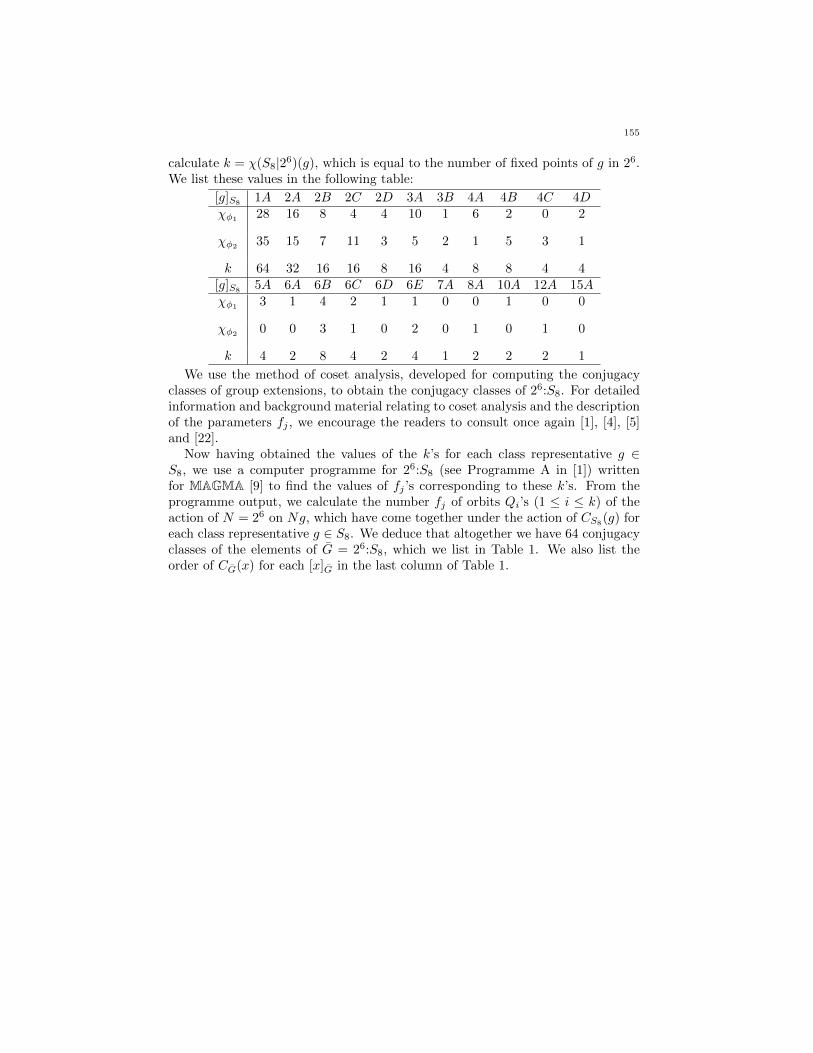
calculate k = χ(S8|26)(g), which is equal to the number of fixed points of g in 26.We list these values in the following table:
[g]S81A 2A 2B 2C 2D 3A 3B 4A 4B 4C 4D
χφ128 16 8 4 4 10 1 6 2 0 2
χφ235 15 7 11 3 5 2 1 5 3 1
k 64 32 16 16 8 16 4 8 8 4 4[g]S8 5A 6A 6B 6C 6D 6E 7A 8A 10A 12A 15Aχφ1
3 1 4 2 1 1 0 0 1 0 0
χφ2 0 0 3 1 0 2 0 1 0 1 0
k 4 2 8 4 2 4 1 2 2 2 1
We use the method of coset analysis, developed for computing the conjugacyclasses of group extensions, to obtain the conjugacy classes of 26:S8. For detailedinformation and background material relating to coset analysis and the descriptionof the parameters fj , we encourage the readers to consult once again [1], [4], [5]and [22].
Now having obtained the values of the k’s for each class representative g ∈S8, we use a computer programme for 26:S8 (see Programme A in [1]) writtenfor MAGMA [9] to find the values of fj ’s corresponding to these k’s. From theprogramme output, we calculate the number fj of orbits Qi’s (1 ≤ i ≤ k) of theaction of N = 26 on Ng, which have come together under the action of CS8
(g) foreach class representative g ∈ S8. We deduce that altogether we have 64 conjugacyclasses of the elements of G = 26:S8, which we list in Table 1. We also list theorder of CG(x) for each [x]G in the last column of Table 1.
155

Table 1: The conjugacy classes of G = 26:S8
[g]S8k fj [x]26:S8
|[x]26:S8| |C26:S8
(x)|1A 64 f1 = 1 1A 1 2580480
f2 = 28 2A 28 92160f3 = 35 2B 35 73728
2A 32 f1 = 1 2C 56 46080f2 = 6 4A 336 7680f3 = 10 4B 560 4608f4 = 15 2D 840 3072
2B 16 f1 = 1 2E 420 6144f2 = 1 2F 420 6144f3 = 2 2G 840 3072f4 = 12 4C 5040 512
2C 16 f1 = 1 2H 840 3072f2 = 1 4D 840 3072f3 = 3 2I 2520 1024f4 = 3 4E 2520 1024f5 = 8 4F 6720 384
2D 8 f1 = 1 2J 3360 768f2 = 1 4G 3360 768f3 = 3 4H 10080 256f4 = 3 4I 10080 256
3A 16 f1 = 1 3A 448 5760f2 = 5 6A 2240 1152f3 = 10 6B 4480 576
156

Table 1: The conjugacy classes of G (continued)
[g]S8k fj [x]26:S8
|[x]26:S8| |C26:S8
(x)|3B 4 f1 = 1 3B 17920 144
f2 = 1 6C 17920 144f3 = 2 6D 35840 72
4A 8 f1 = 1 4J 3360 768f2 = 3 4K 10080 256f3 = 4 8A 13440 192
4B 8 f1 = 1 4L 10080 256f2 = 1 4M 10080 256f3 = 2 4N 20160 128f4 = 4 8B 40320 64
4C 4 f1 = 1 4O 20160 128f2 = 1 4P 20160 128f3 = 2 4Q 40320 64
4D 4 f1 = 1 4R 40320 64f2 = 1 8C 40320 64f3 = 1 8D 40320 64f4 = 1 4S 40320 64
5A 4 f1 = 1 5A 21504 120f2 = 3 10A 64512 40
6A 2 f1 = 1 6E 35840 72f2 = 1 12A 35840 72
6B 8 f1 = 1 6F 8960 288f2 = 1 12B 8960 288f3 = 3 12C 26880 96f4 = 3 6G 26880 96
6C 4 f1 = 1 6H 26880 96f2 = 1 12D 26880 96f3 = 2 12E 53760 48
6D 2 f1 = 1 6I 107520 24f2 = 1 12F 107520 24
6E 4 f1 = 1 6J 53760 48f2 = 1 6K 53760 48f3 = 2 6L 107520 24
7A 1 f1 = 1 7A 368640 7
8A 2 f1 = 1 8E 161280 16f2 = 1 8F 161280 16
10A 2 f1 = 1 10B 129024 20f2 = 1 20A 129024 20
12A 2 f1 = 1 12G 107520 24f2 = 1 24A 107520 24
15A 1 f1 = 1 15A 172032 15
3. The Inertia Groups of G
The action of G on N produces three orbits of lengths 1, 28 and 35. Hence byBrauer’s theorem (see Lemma 4.5.2 of [14]) G acting on Irr(N) will also producethree orbits of lengths 1, s and t such that s+ t = 63. From ATLAS, by checkingthe indices of maximal subgroups of S8, we can see that the only possibility isthat s = 28 and t = 35. We deduce that the three inertia groups are Hi = 26:Hi
of indices 1, 28 and 35 in G respectively where i ∈ 1, 2, 3 and Hi ≤ S8 are theinertia factors. We also observe that H1 = S8, H2 = S6×2 and H3 = (S4×S4):2.
157

The character tables and power maps of the elements of H1, H2 and H3 are givenin the GAP [29]. Using the permutation characters of S8 on H2 and H3 of degrees28 and 35 respectively we are able to obtain partial fusions of H2 and H3 intoH1 = S8. We completed the fusions by using direct matrix conjugation in S8. Thecomplete fusion of H2 and H3 into H1 are given in Tables 2 and 3 respectively.
Table 2: The fusion of H2 into H1
[g]S6×2 −→ [h]S8[g]S6×2 −→ [h]S8
1A 1A 2A 2A2B 2A 2C 2D2D 2B 2E 2C2F 2C 2G 2D3A 3A 3B 3B4A 4D 4B 4A4C 4B 4D 4D5A 5A 6A 6B6B 6A 6C 6B6D 6E 6E 6D6F 6C 10A 10A
Table 3: The fusion of H3 into H1
[g]S4×S4−→ [h]S8
[g]S4×S4−→ [h]S8
1A 1A 2A 2C2B 2B 2C 2A2D 2B 2E 2C2F 2D 3A 3A3B 3B 4A 4A4B 4C 4C 4B4D 4C 4E 4D4F 4B 6A 6C6B 6B 6C 6E8A 8A 12A 12A
4. The Fischer-Clifford Matrices of G
For each conjugacy class [g] of G with representative g ∈ G, we construct thecorresponding Fischer-Clifford matrix M(g) of G = 26:S8. We use properties ofthe Fischer-Clifford matrices (see [1], [3], [4], [5], [22]) together with fusions of H2
and H3 into H1 (Tables 2 and 3) to compute the entries of the these matrices. TheFischer-Clifford matrix M(g) will be partitioned row-wise into blocks, where eachblock corresponds to an inertia group Hi. We list the Fischer-Clifford matrices ofG in Table 4.
158

Table 4: The Fischer-Clifford matrices of G
M(g) M(g) M(g)
M(1A) =
1 1 128 4 −435 −5 3
M(2A) =
1 1 1 11 −1 −1 1
15 5 −3 −115 −5 3 −1
M(2B) =
1 1 1 14 4 −4 03 3 3 −18 −8 0 0
M(2C) =
1 1 1 1 12 −2 −2 2 06 6 −2 −2 01 1 1 1 −16 −6 2 −2 0
M(2D) =
1 1 1 11 −1 −1 13 −3 1 −13 3 −1 −1
M(3A) =
1 1 110 2 −25 −3 1
M(3B) =
1 1 11 1 −12 −2 0
M(4A) =
1 1 16 −2 01 1 −1
M(4B) =
1 1 1 12 2 −2 01 1 1 −14 −4 0 0
M(4C) =
1 1 11 1 −12 −2 0
M(4D) =
1 1 1 11 1 −1 −11 −1 −1 11 −1 1 −1
M(5A) =
(1 13 −1
)
M(6A) =
(1 11 −1
)M(6B) =
1 1 1 11 −1 −1 13 3 −1 −13 −3 1 −1
M(6C) =
1 1 12 −2 01 1 −1
M(6D) =
(1 11 −1
)M(6E) =
1 1 11 1 −12 −2 0
M(7A) =
(1)
M(8A) =
(1 11 −1
)M(10A) =
(1 11 −1
)M(12A) =
(1 11 −1
)
M(15A) =(
1)
We use the above Fischer-Clifford matrices (Table 4) and the character tablesof inertia factor groups H1 = S8, H2 and H3, together with the fusion of H2 andH3 into S8, to obtain the character table of G. The set of irreducible charactersof G = 26:S8 will be partitioned into three blocks B1, B2 and B3 correspondingto the inertia factors H1, H2 and H3 respectively. In fact B1 = χi| 1 ≤ i ≤ 22,B2 = χi| 23 ≤ i ≤ 44 and B3 = χi| 45 ≤ i ≤ 64, where Irr(26:S8) =
⋃3i=1Bi.
The character table of G is displayed in Table 5. Note that the centralizers of theelements of G are listed in the last column of Table 1.
The character table of G = 26:S8, which we computed in this paper and dis-played in Table 5, has been incorporated into and available in the latest versionof GAP [29] as well.
159

Table 5: The character table of G
[g]S81A 2A 2B 2C
[x]26:S81A 2A 2B 2C 4A 4B 2D 2E 2F 2G 4C 2H 4D 2I 4E 4F
χ1 1 1 1 1 1 1 1 1 1 1 1 1 1 1 1 1χ2 1 1 1 -1 -1 -1 -1 1 1 1 1 1 1 1 1 1χ3 7 7 7 5 5 5 5 -1 -1 -1 -1 3 3 3 3 3χ4 7 7 7 -5 -5 -5 -5 -1 -1 -1 -1 3 3 3 3 3χ5 14 14 14 4 4 4 4 4 6 6 6 6 2 2 2 2χ6 14 14 14 -4 -4 -4 -4 4 6 6 6 6 2 2 2 2χ7 20 20 20 10 10 10 10 4 4 4 4 4 4 4 4 4χ8 20 20 20 -10 -10 -10 -10 4 4 4 4 4 4 4 4 4χ9 21 21 21 9 9 9 9 -3 -3 -3 -3 1 1 1 1 1χ10 21 21 21 -9 -9 -9 -9 -3 -3 -3 -3 1 1 1 1 1χ11 42 42 42 0 0 0 0 -6 -6 -6 -6 2 2 2 2 2χ12 28 28 28 10 10 10 10 -4 -4 -4 -4 4 4 4 4 4χ13 28 28 28 -10 -10 -10 -10 -4 -4 -4 -4 4 4 4 4 4χ14 35 35 35 5 5 5 5 3 3 3 3 -5 -5 -5 -5 -5χ15 35 35 35 -5 -5 -5 -5 3 3 3 3 -5 -5 -5 -5 -5χ16 90 90 90 0 0 0 0 -6 -6 -6 -6 -6 -6 -6 -6 -6χ17 56 56 56 4 4 4 4 8 8 8 8 0 0 0 0 0χ18 56 56 56 -4 -4 -4 -4 8 8 8 8 0 0 0 0 0χ19 64 64 64 16 16 16 16 0 0 0 0 0 0 0 0 0χ20 64 64 64 -16 -16 -16 -16 0 0 0 0 0 0 0 0 0χ21 70 70 70 10 10 10 10 -2 -2 -2 -2 2 2 2 2 2χ22 70 70 70 -10 -10 -10 -10 -2 -2 -2 -2 2 2 2 2 2χ23 28 4 -4 16 4 -4 0 4 4 -4 0 8 4 0 -4 0χ24 28 4 -4 14 6 -2 -2 -4 -4 4 0 4 8 -4 0 0χ25 28 4 -4 -16 -4 4 0 4 4 -4 0 8 4 0 -4 0χ26 28 4 -4 -14 -6 2 2 -4 -4 4 0 4 8 -4 0 0χ27 140 20 -20 -40 -20 4 8 4 4 -4 0 0 12 -8 4 0χ28 140 20 -20 40 20 -4 -8 4 4 -4 0 0 12 -8 4 0χ29 140 20 -20 50 10 -14 2 -4 -4 4 0 12 0 4 -8 0χ30 140 20 -20 -50 -10 14 -2 -4 -4 4 0 12 0 4 -8 0χ31 140 20 -20 20 0 -8 4 -12 -12 12 0 8 4 0 -4 0χ32 140 20 -20 -20 0 8 -4 -12 -12 12 0 8 4 0 -4 0
160
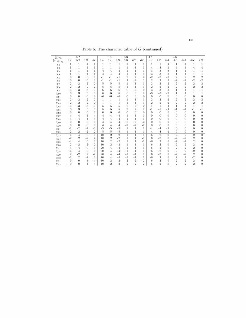
Table 5: The character table of G (continued)
[g]S82D 3A 3B 4A 4B
[x]26:S82J 4G 4H 4I 3A 6A 6B 3B 6C 6D 4J 4K 8A 4L 4M 4N 8B
χ1 1 1 1 1 1 1 1 1 1 1 1 1 1 1 1 1 1χ2 -1 -1 -1 -1 1 1 1 1 1 1 -4 -4 -4 -4 -4 -4 -4χ3 1 1 1 1 4 4 4 1 1 1 3 3 3 -1 -1 -1 -1χ4 -1 -1 -1 -1 4 4 4 1 1 1 -3 -3 -3 1 1 1 1χ5 0 0 0 0 -1 -1 -1 2 2 2 -2 -2 -2 2 2 2 2χ6 0 0 0 0 -1 -1 -1 2 2 2 2 2 2 -2 -2 -2 -2χ7 2 2 2 2 5 5 5 -1 -1 -1 2 2 2 2 2 2 2χ8 -2 -2 -2 -2 5 5 5 -1 -1 -1 -2 -2 -2 -2 -2 -2 -2χ9 -3 -3 -3 -3 6 6 6 0 0 0 3 3 3 -1 -1 -1 -1χ10 3 3 3 3 6 6 6 0 0 0 -3 -3 -3 1 1 1 1χ11 0 0 0 0 -6 -6 -6 0 0 0 0 0 0 0 0 0 0χ12 2 2 2 2 1 1 1 1 1 1 -2 -2 -2 -2 -2 -2 -2χ13 -2 -2 -2 -2 1 1 1 1 1 1 2 2 2 2 2 2 2χ14 -3 -3 -3 -3 5 5 5 2 2 2 1 1 1 1 1 1 1χ15 3 3 3 3 5 5 5 2 2 2 -1 -1 -1 -1 -1 -1 -1χ16 0 0 0 0 0 0 0 0 0 0 0 0 0 0 0 0 0χ17 4 4 4 4 -4 -4 -4 -1 -1 -1 0 0 0 0 0 0 0χ18 -4 -4 -4 -4 -4 -4 -4 -1 -1 -1 0 0 0 0 0 0 0χ19 0 0 0 0 4 4 4 -2 -2 -2 0 0 0 0 0 0 0χ20 0 0 0 0 4 4 4 -2 -2 -2 0 0 0 0 0 0 0χ21 -2 -2 -2 -2 -5 -5 -5 1 1 1 -4 -4 -4 0 0 0 0χ22 2 2 2 2 -5 -5 -5 1 1 1 4 4 4 0 0 0 0χ23 4 -4 0 0 10 2 -2 1 1 -1 6 -2 0 2 2 -2 0χ24 -2 2 -2 2 10 2 -2 1 1 -1 6 -2 0 -2 -2 2 0χ25 -4 4 0 0 10 2 -2 1 1 -1 -6 2 0 -2 -2 2 0χ26 2 -2 2 -2 10 2 -2 1 1 -1 -6 2 0 2 2 -2 0χ27 4 -4 0 0 20 4 -4 -1 -1 1 -6 2 0 -2 -2 2 0χ28 -4 4 0 0 20 4 -4 -1 -1 1 6 -2 0 2 2 -2 0χ29 2 -2 2 -2 20 4 -4 -1 -1 1 6 -2 0 -2 -2 2 0χ30 -2 2 -2 2 20 4 -4 -1 -1 1 -6 2 0 2 2 -2 0χ31 0 0 4 -4 -10 -2 2 2 2 -2 -6 2 0 -2 -2 2 0χ32 0 0 -4 4 -10 -2 2 2 2 -2 6 -2 0 2 2 -2 0
161
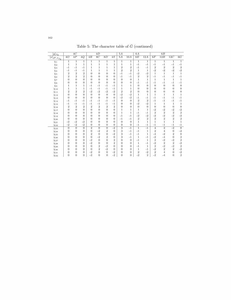
Table 5: The character table of G (continued)
[g]S84C 4D 5A 6A 6B
[x]26:SS84O 4P 4Q 4R 8C 8D 4S 5A 10A 6E 12A 6F 12B 12C 6G
χ1 1 1 1 1 1 1 1 1 1 1 1 1 1 1 1χ2 1 1 1 1 1 1 1 1 1 -1 -1 -1 -1 -1 -1χ3 -1 -1 -1 1 1 1 1 2 2 -1 -1 2 2 2 2χ4 -1 -1 -1 1 1 1 1 2 2 1 1 -2 -2 -2 -2χ5 2 2 2 0 0 0 0 -1 -1 -2 -2 1 1 1 1χ6 2 2 2 0 0 0 0 -1 -1 2 2 -1 -1 -1 -1χ7 0 0 0 0 0 0 0 0 0 1 1 1 1 1 1χ8 0 0 0 0 0 0 0 0 0 -1 -1 -1 -1 -1 -1χ9 1 1 1 -1 -1 -1 -1 1 1 0 0 0 0 0 0χ10 1 1 1 -1 -1 -1 -1 1 1 0 0 0 0 0 0χ11 2 2 2 -2 -2 -2 -2 2 2 0 0 0 0 0 0χ12 0 0 0 0 0 0 0 -2 -2 1 1 1 1 1 1χ13 0 0 0 0 0 0 0 -2 -2 -1 -1 -1 -1 -1 -1χ14 -1 -1 -1 -1 -1 -1 -1 0 0 2 2 -1 -1 -1 -1χ15 -1 -1 -1 -1 -1 -1 -1 0 0 -2 -2 1 1 1 1χ16 2 2 2 2 2 2 2 0 0 0 0 0 0 0 0χ17 0 0 0 0 0 0 0 1 1 1 1 -2 -2 -2 -2χ18 0 0 0 0 0 0 0 1 1 -1 -1 2 2 2 2χ19 0 0 0 0 0 0 0 -1 -1 -2 -2 -2 -2 -2 -2χ20 0 0 0 0 0 0 0 -1 -1 2 2 2 2 2 2χ21 -2 -2 -2 0 0 0 0 0 0 1 1 1 1 1 1χ22 -2 -2 -2 0 0 0 0 0 0 -1 -1 -1 -1 -1 -1χ23 0 0 0 2 0 0 -2 3 -1 1 -1 4 2 -2 0χ24 0 0 0 0 -2 2 0 3 -1 -1 1 2 4 0 -2χ25 0 0 0 2 0 0 -2 3 -1 -1 1 -4 -2 2 0χ26 0 0 0 0 -2 2 0 3 -1 1 -1 -2 -4 0 2χ27 0 0 0 -2 0 0 2 0 0 -1 1 2 -2 -2 2χ28 0 0 0 -2 0 0 2 0 0 1 -1 -2 2 2 -2χ29 0 0 0 0 2 -2 0 0 0 -1 1 2 -2 -2 2χ30 0 0 0 0 2 -2 0 0 0 1 -1 -2 2 2 -2χ31 0 0 0 -2 0 0 -2 0 0 2 -2 2 4 0 -2χ32 0 0 0 -2 0 0 -2 0 0 -2 2 -2 -4 0 2
162

Table 5: The character table of G (continued)
[g]S86C 6D 6E 7A 8A 10A 12A 15A
[x]26:SS86H 12D 12E 6I 12F 6J 6K 6L 7A 8E 8F 10B 20A 12G 24A 15A
χ1 1 1 1 1 1 1 1 1 1 1 1 1 1 1 1 1χ2 1 1 1 -1 -1 1 1 1 1 -1 -1 -1 -1 -1 -1 1χ3 0 0 0 1 1 -1 -1 -1 0 -1 -1 0 0 0 0 -1χ4 0 0 0 -1 -1 -1 -1 -1 0 1 1 0 0 0 0 -1χ5 -1 -1 -1 0 0 0 0 0 0 0 0 -1 -1 1 1 -1χ6 -1 -1 -1 0 0 0 0 0 0 0 0 1 1 -1 -1 -1χ7 1 1 1 -1 -1 1 1 1 -1 0 0 0 0 -1 -1 0χ8 1 1 1 1 1 1 1 1 -1 0 0 0 0 1 1 0χ9 -2 -2 -2 0 0 0 0 0 0 1 1 -1 -1 0 0 1χ10 -2 -2 -2 0 0 0 0 0 0 -1 -1 1 1 0 0 1χ11 2 2 2 0 0 0 0 0 0 0 0 0 0 0 0 -1χ12 1 1 1 -1 -1 -1 -1 -1 0 0 0 0 0 1 1 1χ13 1 1 1 1 1 -1 -1 -1 0 0 0 0 0 -1 -1 1χ14 1 1 1 0 0 0 0 0 0 -1 -1 0 0 1 1 0χ15 1 1 1 0 0 0 0 0 0 1 1 0 0 -1 -1 0χ16 0 0 0 0 0 0 0 0 -1 0 0 0 0 0 0 0χ17 0 0 0 1 1 -1 -1 -1 0 0 0 -1 -1 0 0 1χ18 0 0 0 -1 -1 -1 -1 -1 0 0 0 1 1 0 0 1χ19 0 0 0 0 0 0 0 0 1 0 0 1 1 0 0 -1χ20 0 0 0 0 0 0 0 0 1 0 0 -1 -1 0 0 -1χ21 -1 -1 -1 1 1 1 1 1 0 0 0 0 0 -1 -1 0χ22 -1 -1 -1 -1 -1 1 1 1 0 0 0 0 0 1 1 0χ23 2 -2 0 1 -1 1 1 -1 0 0 0 1 -1 0 0 0χ24 -2 2 0 1 -1 -1 -1 1 0 0 0 -1 1 0 0 0χ25 2 -2 0 -1 1 1 1 -1 0 0 0 -1 1 0 0 0χ26 -2 2 0 -1 1 -1 -1 1 0 0 0 1 -1 0 0 0χ27 0 0 0 1 -1 1 1 -1 0 0 0 0 0 0 0 0χ28 0 0 0 -1 1 1 1 -1 0 0 0 0 0 0 0 0χ29 0 0 0 -1 1 -1 -1 1 0 0 0 0 0 0 0 0χ30 0 0 0 1 -1 -1 -1 1 0 0 0 0 0 0 0 0χ31 2 -2 0 0 0 0 0 0 0 0 0 0 0 0 0 0χ32 2 -2 0 0 0 0 0 0 0 0 0 0 0 0 0 0
163

Table 5: The character table of G (continued)
[g]S81A 2A 2B 2C
[x]26:S81A 2A 2B 2C 4A 4B 2D 2E 2F 2G 4C 2H 4D 2I 4E 4F
χ33 140 20 -20 10 10 2 -6 12 12 -12 0 4 8 -4 0 0χ34 140 20 -20 -10 -10 -2 6 12 12 -12 0 4 8 -4 0 0χ35 452 36 -36 -36 -24 0 12 -12 -12 12 0 0 12 -8 4 0χ36 452 36 -36 36 24 0 -12 -12 -12 12 0 0 12 -8 4 0χ37 452 36 -36 54 6 -18 6 12 12 -12 0 12 0 4 -8 0χ38 452 36 -36 -54 -6 18 -6 12 12 -12 0 12 0 4 -8 0χ39 280 40 -40 40 0 -16 8 -8 -8 8 0 -8 -16 8 0 0χ40 280 40 -40 -40 0 16 -8 -8 -8 8 0 -8 -16 8 0 0χ41 280 40 -40 20 20 4 -12 8 8 -8 0 -16 -8 0 8 0χ42 280 40 -40 -20 -20 -4 12 8 8 -8 0 -16 -8 0 8 0χ43 448 64 -64 16 -16 -16 16 0 0 0 0 0 0 0 0 0χ44 448 64 -64 -16 16 16 -16 0 0 0 0 0 0 0 0 0χ45 35 -5 3 15 -5 3 -1 11 -5 3 -1 7 -5 -1 3 -1χ46 35 -5 3 -15 5 -3 1 -5 11 3 -1 7 -5 -1 3 -1χ47 35 -5 3 -15 5 -3 1 11 -5 3 -1 7 -5 -1 3 -1χ48 35 -5 3 15 -5 3 -1 -5 11 3 -1 7 -5 -1 3 -1χ49 70 -10 6 0 0 0 0 6 6 6 -2 -10 14 6 -2 -2χ50 140 -20 12 -30 10 -6 2 12 12 12 -4 4 4 4 4 -4χ51 140 -20 12 30 -10 6 -2 12 12 12 -4 4 4 4 4 -4χ52 140 -20 12 0 0 0 0 -4 28 12 -4 4 4 4 4 -4χ53 140 -20 12 0 0 0 0 28 -4 12 -4 4 4 4 4 -4χ54 210 -30 18 -30 10 -6 2 -6 -6 -6 2 -10 14 6 -2 -2χ55 210 -30 18 30 -10 6 -2 -6 -6 -6 2 -10 14 6 -2 -2χ56 210 -30 18 -60 20 -12 4 -6 -6 -6 2 14 -10 -2 6 -2χ57 210 -30 18 60 -20 12 -4 -6 -6 -6 2 14 -10 -2 6 -2χ58 315 -45 27 -45 15 -9 3 -21 27 3 -1 3 -9 -5 -1 3χ59 315 -45 27 -45 15 -9 3 27 -21 3 -1 3 -9 -5 -1 3χ60 315 -45 27 45 -15 9 -3 -21 27 3 -1 3 -9 -5 -1 3χ61 315 -45 27 45 -15 9 -3 27 -21 3 -1 3 -9 -5 -1 3χ62 420 -60 36 -30 10 -6 2 -12 -12 -12 4 4 4 4 4 -4χ63 420 -60 36 30 -10 6 -2 -12 -12 -12 4 4 4 4 4 -4χ64 630 -90 54 0 0 0 0 6 6 6 -2 -18 6 -2 -10 6
164

Table 5: The character table of G (continued)
[g]S82D 3A 3B 4A 4B
[x]26:S82J 4G 4H 4I 3A 6A 6B 3B 6C 6D 4J 4K 8A 4L 4M 4N 8B
χ33 -6 6 2 -2 -10 -2 2 2 2 -2 -6 2 0 2 2 -2 0χ34 6 -6 -2 2 -10 -2 2 2 2 -2 6 -2 0 -2 -2 2 0χ35 0 0 4 -4 0 0 0 0 0 0 6 -2 0 2 2 -2 0χ36 0 0 -4 4 0 0 0 0 0 0 -6 2 0 -2 -2 2 0χ37 6 -6 -2 2 0 0 0 0 0 0 -6 2 0 2 2 -2 0χ38 -6 6 2 -2 0 0 0 0 0 0 6 -2 0 -2 -2 2 0χ39 -8 8 0 0 10 2 -2 1 1 -1 0 0 0 0 0 0 0χ40 8 -8 0 0 10 2 -2 1 1 -1 0 0 0 0 0 0 0χ41 4 -4 4 -4 10 2 -2 1 1 -1 0 0 0 0 0 0 0χ42 -4 4 -4 4 10 2 -2 1 1 -1 0 0 0 0 0 0 0χ43 0 0 0 0 -20 -4 4 -2 -2 2 0 0 0 0 0 0 0χ44 0 0 0 0 -20 -4 4 -2 -2 2 0 0 0 0 0 0 0χ45 3 3 -1 -1 5 -3 1 2 -2 0 1 1 -1 5 -3 1 -1χ46 -3 -3 1 1 5 -3 1 2 -2 0 -1 -1 1 3 -5 -1 1χ47 -3 -3 1 1 5 -3 1 2 -2 0 -1 -1 1 -5 3 -1 1χ48 3 3 -1 -1 5 -3 1 2 -2 0 1 1 -1 -3 5 1 -1χ49 0 0 0 0 10 -6 2 4 -4 0 0 0 0 0 0 0 0χ50 -6 -6 2 2 5 -3 1 -4 4 0 -2 -2 2 -2 -2 -2 2χ51 6 6 -2 -2 5 -3 1 -4 4 0 2 2 -2 2 2 2 -2χ52 0 0 0 0 -10 6 -2 2 -2 0 0 0 0 0 0 0 0χ53 0 0 0 0 -10 6 -2 2 -2 0 0 0 0 0 0 0 0χ54 6 6 -2 -2 15 -9 3 0 0 0 -4 -4 4 0 0 0 0χ55 -6 -6 2 2 15 -9 3 0 0 0 4 4 -4 0 0 0 0χ56 0 0 0 0 15 -9 3 0 0 0 -2 -2 2 2 2 2 -2χ57 0 0 0 0 15 -9 3 0 0 0 2 2 -2 -2 -2 -2 2χ58 3 3 -1 -1 0 0 0 0 0 0 3 3 -3 3 -5 -1 1χ59 3 3 -1 -1 0 0 0 0 0 0 3 3 -3 -5 3 -1 1χ60 -3 -3 1 1 0 0 0 0 0 0 -3 -3 3 -3 5 1 -1χ61 -3 -3 1 1 0 0 0 0 0 0 -3 -3 3 5 -3 1 -1χ62 -6 -6 2 2 -15 9 -3 0 0 0 2 2 -2 2 2 2 -2χ63 6 6 -2 -2 -15 9 -3 0 0 0 -2 -2 2 -2 -2 -2 2χ64 0 0 0 0 0 0 0 0 0 0 0 0 0 0 0 0 0
165

Table 5: The character table of G (continued)
[g]S84C 4D 5A 6A 6B
[x]26:SS84O 4P 4Q 4R 8C 8D 4S 5A 10A 6E 12A 6F 12B 12C 6G
χ33 0 0 0 0 2 -2 0 0 0 -2 2 4 2 -2 0χ34 0 0 0 0 2 -2 0 0 0 2 -2 -4 -2 2 0χ35 0 0 0 2 0 0 -2 -3 1 0 0 0 0 0 0χ36 0 0 0 2 0 0 -2 -3 1 0 0 0 0 0 0χ37 0 0 0 0 -2 2 0 -3 1 0 0 0 0 0 0χ38 0 0 0 0 -2 2 0 -3 1 0 0 0 0 0 0χ39 0 0 0 0 0 0 0 0 0 1 -1 -2 -4 0 2χ40 0 0 0 0 0 0 0 0 0 -1 1 2 4 0 -2χ41 0 0 0 0 0 0 0 0 0 -1 1 -4 -2 2 0χ42 0 0 0 0 0 0 0 0 0 1 -1 4 2 -2 0χ43 0 0 0 0 0 0 0 3 -1 -2 2 -2 2 2 -2χ44 0 0 0 0 0 0 0 3 -1 2 -2 2 -2 -2 2χ45 3 -1 -1 1 -1 -1 1 0 0 0 0 3 -3 1 -1χ46 -1 3 -1 1 -1 -1 1 0 0 0 0 -3 3 -1 1χ47 3 -1 -1 1 -1 -1 1 0 0 0 0 -3 3 -1 1χ48 -1 3 -1 1 -1 -1 1 0 0 0 0 3 -3 1 -1χ49 -2 -2 2 -2 2 2 -2 0 0 0 0 0 0 0 0χ50 0 0 0 0 0 0 0 0 0 0 0 3 -3 1 -1χ51 0 0 0 0 0 0 0 0 0 0 0 -3 3 -1 1χ52 -4 4 0 0 0 0 0 0 0 0 0 0 0 0 0χ53 4 -4 0 0 0 0 0 0 0 0 0 0 0 0 0χ54 2 2 -2 0 0 0 0 0 0 0 0 3 -3 1 -1χ55 2 2 -2 0 0 0 0 0 0 0 0 -3 3 -1 1χ56 -2 -2 2 0 0 0 0 0 0 0 0 -3 3 -1 1χ57 -2 -2 2 0 0 0 0 0 0 0 0 3 -3 1 -1χ58 3 -1 -1 -1 1 1 -1 0 0 0 0 0 0 0 0χ59 -1 3 -1 -1 1 1 -1 0 0 0 0 0 0 0 0χ60 3 -1 -1 -1 1 1 -1 0 0 0 0 0 0 0 0χ61 -1 3 -1 -1 1 1 -1 0 0 0 0 0 0 0 0χ62 0 0 0 0 0 0 0 0 0 0 0 3 -3 1 -1χ63 0 0 0 0 0 0 0 0 0 0 0 -3 3 -1 1χ64 -2 -2 2 2 -2 -2 2 0 0 0 0 0 0 0 0
166

Table 5: The character table of G (continued)
[g]S86C 6D 6E 7A 8A 10A 12A 15A
[x]26:SS86H 12D 12E 6I 12F 6J 6K 6L 7A 8E 8F 10B 20A 12G 24A 15A
χ33 -2 2 0 0 0 0 0 0 0 0 0 0 0 0 0 0χ34 -2 2 0 0 0 0 0 0 0 0 0 0 0 0 0 0χ35 0 0 0 0 0 0 0 0 0 0 0 -1 1 0 0 0χ36 0 0 0 0 0 0 0 0 0 0 0 1 -1 0 0 0χ37 0 0 0 0 0 0 0 0 0 0 0 -1 1 0 0 0χ38 0 0 0 0 0 0 0 0 0 0 0 1 -1 0 0 0χ39 -2 2 0 1 -1 1 1 -1 0 0 0 0 0 0 0 0χ40 -2 2 0 -1 1 1 1 -1 0 0 0 0 0 0 0 0χ41 2 -2 0 1 -1 -1 -1 1 0 0 0 0 0 0 0 0χ42 2 -2 0 -1 1 -1 -1 1 0 0 0 0 0 0 0 0χ43 0 0 0 0 0 0 0 0 0 0 0 1 -1 0 0 0χ44 0 0 0 0 0 0 0 0 0 0 0 -1 1 0 0 0χ45 1 1 -1 0 0 2 -2 0 0 1 -1 0 0 1 -1 0χ46 1 1 -1 0 0 -2 2 0 0 1 -1 0 0 -1 1 0χ47 1 1 -1 0 0 2 -2 0 0 -1 1 0 0 -1 1 0χ48 1 1 -1 0 0 -2 2 0 0 -1 1 0 0 1 -1 0χ49 2 2 -2 0 0 0 0 0 0 0 0 0 0 0 0 0χ50 1 1 -1 0 0 0 0 0 0 0 0 0 0 1 -1 0χ51 1 1 -1 0 0 2 -2 0 0 1 -1 0 0 -1 1 0χ52 -2 -2 2 0 0 2 -2 0 0 0 0 0 0 0 0 0χ53 -2 -2 2 0 0 -2 2 0 0 0 0 0 0 0 0 0χ54 -1 -1 1 0 0 0 0 0 0 0 0 0 0 -1 1 0χ55 -1 -1 1 0 0 0 0 0 0 0 0 0 0 1 -1 0χ56 -1 -1 1 0 0 0 0 0 0 0 0 0 0 1 -1 0χ57 -1 -1 1 0 0 0 0 0 0 0 0 0 0 -1 1 0χ58 0 0 0 0 0 0 0 0 0 -1 1 0 0 0 0 0χ59 0 0 0 0 0 0 0 0 0 1 -1 0 0 0 0 0χ60 0 0 0 0 0 0 0 0 0 1 -1 0 0 0 0 0χ61 0 0 0 0 0 0 0 0 0 -1 1 0 0 0 0 0χ62 1 1 -1 0 0 0 0 0 0 0 0 0 0 -1 1 0χ63 1 1 -1 0 0 0 0 0 0 0 0 0 0 1 -1 0χ64 0 0 0 0 0 0 0 0 0 0 0 0 0 0 0 0
5. The Fusion of G into Fi22
We use the results of the conjugacy classes of G which are given in Section 2,to compute the power maps of the elements of G which we list in Table 6.
167

Table 6: The power maps of the elements of G
[g]S8[x]26:S8
2 3 5 7 [g]S8[x]26:S8
2 3 5 7
1A 1A 2A 2C 1A2A 1A 4A 2A2B 1A 4B 2A
2D 1A2B 2E 1A 2C 2H 1A
2F 1A 4D 2B2G 1A 2I 1A4C 2B 4E 2B
4F 2A2D 2J 1A 3A 3A 1A
4G 2A 6A 3A 2B4H 2A 6B 3A 2A4I 2B
3B 3B 1A 4A 4J 2H6C 3B 2A 4K 2H6D 3B 2B 8A 4D
4B 4L 2H 4C 4O 2E4M 2H 4P 2F4N 2H 4Q 2G8B 4E
4D 4R 2H 5A 5A 1A8C 4D 10A 5A 2A8D 4E4S 2I
6A 6E 3B 2D 6B 6F 3A 2C12A 6C 4B 12B 6B 4B
12C 6B 4A6G 3A 2D
6C 6H 3A 2H 6D 6I 3B 2J12D 6A 4D 12F 6C 4G12E 6B 4F
6E 6J 3B 2E 7A 7A 1A6K 3B 2F6L 3B 2G
8A 8E 4O 10A 10B 5A 2C8F 4P 20A 10A 4A
12A 12G 6H 4J 15A 15A 5A 3A24A 12D 8A
Our group G = 26:S8 sits maximally inside the group E = 26:Sp6(2). Mooriand Mpono in [22] computed the character table of E, which is also available inGAP [29]. The fusion of G into E will help us to determine the fusion of G intoFi22. We give the fusion map of G into E in Table 7.
The power maps of Fi22 are given in the ATLAS and GAP. In order to completethe fusion of G into Fi22 we sometimes use the technique of set intersection. Fordetailed information regarding the technique of set intersection we refer to [1], [4],[5], [21] and [25]. We give the complete list of class fusions of G into Fi22 in Table8.
168
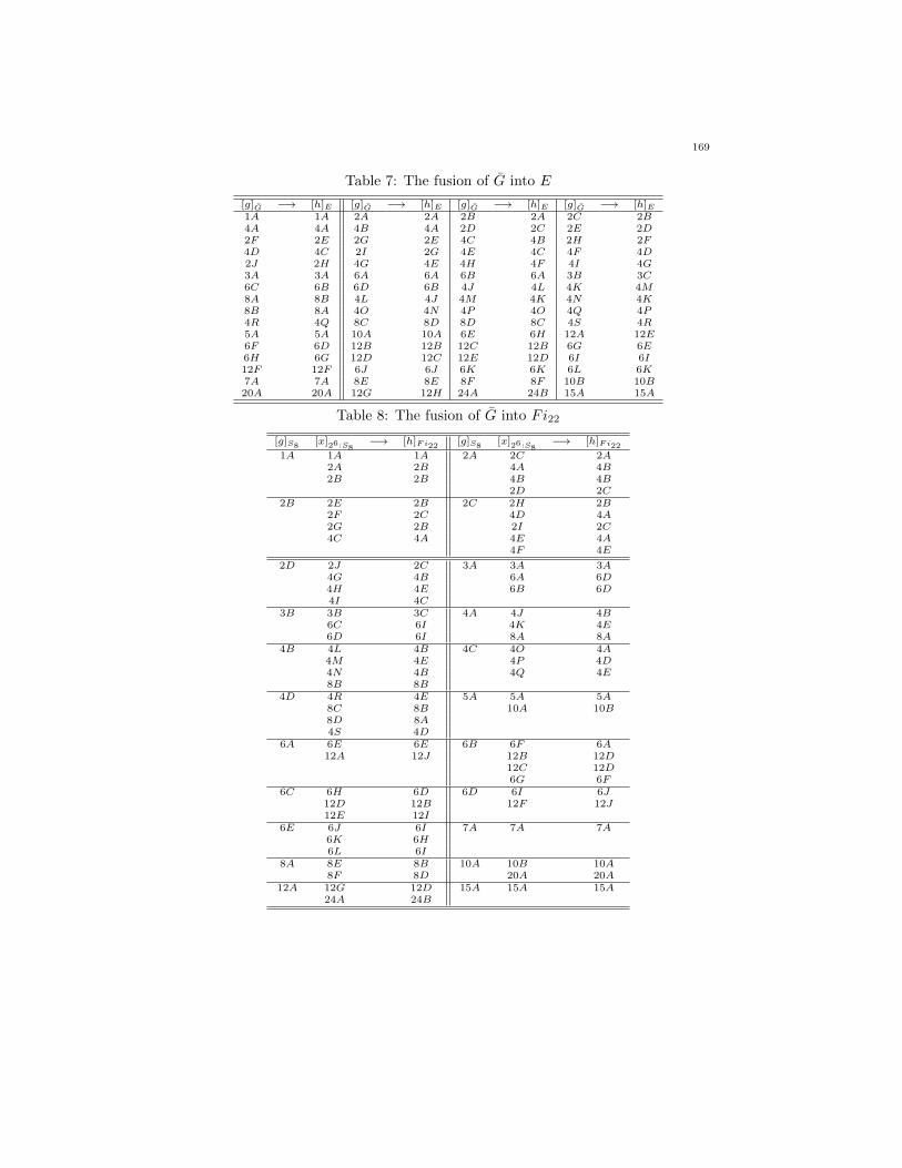
Table 7: The fusion of G into E
[g]G −→ [h]E [g]G −→ [h]E [g]G −→ [h]E [g]G −→ [h]E1A 1A 2A 2A 2B 2A 2C 2B4A 4A 4B 4A 2D 2C 2E 2D2F 2E 2G 2E 4C 4B 2H 2F4D 4C 2I 2G 4E 4C 4F 4D2J 2H 4G 4E 4H 4F 4I 4G3A 3A 6A 6A 6B 6A 3B 3C6C 6B 6D 6B 4J 4L 4K 4M8A 8B 4L 4J 4M 4K 4N 4K8B 8A 4O 4N 4P 4O 4Q 4P4R 4Q 8C 8D 8D 8C 4S 4R5A 5A 10A 10A 6E 6H 12A 12E6F 6D 12B 12B 12C 12B 6G 6E6H 6G 12D 12C 12E 12D 6I 6I12F 12F 6J 6J 6K 6K 6L 6K7A 7A 8E 8E 8F 8F 10B 10B20A 20A 12G 12H 24A 24B 15A 15A
Table 8: The fusion of G into Fi22
[g]S8[x]26:S8
−→ [h]Fi22[g]S8
[x]26:S8−→ [h]Fi22
1A 1A 1A 2A 2C 2A2A 2B 4A 4B2B 2B 4B 4B
2D 2C2B 2E 2B 2C 2H 2B
2F 2C 4D 4A2G 2B 2I 2C4C 4A 4E 4A
4F 4E
2D 2J 2C 3A 3A 3A4G 4B 6A 6D4H 4E 6B 6D4I 4C
3B 3B 3C 4A 4J 4B6C 6I 4K 4E6D 6I 8A 8A
4B 4L 4B 4C 4O 4A4M 4E 4P 4D4N 4B 4Q 4E8B 8B
4D 4R 4E 5A 5A 5A8C 8B 10A 10B8D 8A4S 4D
6A 6E 6E 6B 6F 6A12A 12J 12B 12D
12C 12D6G 6F
6C 6H 6D 6D 6I 6J12D 12B 12F 12J12E 12I
6E 6J 6I 7A 7A 7A6K 6H6L 6I
8A 8E 8B 10A 10B 10A8F 8D 20A 20A
12A 12G 12D 15A 15A 15A24A 24B
169
Acknowledgements
The authors are grateful to the referee for careful reading of the manuscript andfor helpful comments.
References
[1] F. Ali, Fischer-Clifford matrices for split and non-split group extensions, PhD Thesis, Uni-
versity of Natal, Pietermaritzburg, 2001.
[2] F. Ali, The Fischer-Clifford matrices of a maximal subgroup of the sporadic simple group ofHeld, Algebra Colloq., 14 (2007), 135–142.
[3] F. Ali and J. Moori, The Fischer-Clifford matrices of a maximal subgroup of Fi′24, Represent.Theory 7 (2003), 300-321.
[4] F. Ali and J. Moori, Fischer-Clifford matrices of the group 27:Sp6(2), Intl. J. Maths. Game
Theory, and Algebra, 14 (2004), 101-121.[5] F. Ali and J. Moori, Fischer-Clifford matrices and character table of the group 28:Sp6(2),
Intl. J. Maths. Game Theory, and Algebra, 14 (2004), 123-135.
[6] F. Ali and J. Moori, The Fischer-Clifford matrices and character table of a non-split groupextension 26·U4(2) , Quaest. Math. 31 (2008), no. 1, 27–36.
[7] F. Ali and J. Moori, The Fischer-Clifford matrices and character table of a maximal subgroup
of Fi24 , Algebra Colloq., 17 (2010), no. 3, 389–414.[8] S. Ariki and K. Koike, A Hecke algebra of Z/rZ o Sn and construction of its irreducible
representations, Adv. Math. 106(1994), 216-243.
[9] Wieb Bosma and John Cannon. Handbook of Magma functions, Department of Mathematics,University of Sydney, November 1994.
[10] J. H. Conway, R. T. Curtis, S. P. Norton, R. A. Parker, and R. A. Wilson. An Atlas ofFinite Groups, Oxford University Press, 1985.
[11] M. R. Darafsheh and A. Iranmanesh, Computation of the character table of affine groups
using Fischer matrices, London Mathematical Society Lecture Note Series 211, Vol. 1, C.M. Campbell et al., Cambridge University Press (1995), 131 - 137.
[12] B. Fischer, Clifford - matrices, Progr. Math. 95, Michler G. O. and Ringel C. M. (eds),
Birkhauser, Basel (1991), 1 - 16.[13] B. Fischer, Character tables of maximal subgroups of sporadic simple groups -III, Preprint.
[14] D. Gorenstein, Finite Groups, Harper and Row Publishers, New York, 1968.
[15] B. Huppert, Character Theory of Finite Groups, Walter de Gruyter, Berlin, 1998.[16] A. Iranmanesh, Fischer matrices of the affine groups, Southeast Asian Bull. Math. 25
(2001), no. 1, 121–128.
[17] I. M. Isaacs, Character Theory of Finite Groups, Academic Press, San Diego, 1976.[18] C. Jansen, K. Lux, R. Parker and R. Wilson, An Atlas of Brauer Characters, London
Mathematical Society Monographs New Series 11, Oxford University Press, Oxford, 1995.[19] R. J. List, On the characters of 2n−ε.Sn, Arch. Math. 51 (1988), 118-124.
[20] R. J. List and I. M. I. Mahmoud, Fischer matrices for wreath products G w Sn, Arch. Math.
50 (1988), 394-401.[21] J. Moori, On the groups G+ and G of the forms 210:M22 and 210:M22, PhD thesis, Uni-
versity of Birmingham, 1975.
[22] J. Moori and Z.E. Mpono, The Fischer-Clifford matrices of the group 26:SP6(2), Quaes-tiones Math. 22 (1999), 257-298.
[23] J. Moori and Z.E. Mpono, The centralizer of an involutory outer automorphism of F22,
Math. Japonica 49 (1999), 93-113.[24] J. Moori and Z.E. Mpono, Fischer-Clifford matrices and the character table of a maximal
subgroup of F22, Intl. J. Maths. Game Theory, and Algebra 10 (2000), 1-12.
[25] Z. E. Mpono, Fischer-Clifford theory and character tables of group extensions, PhD thesis,University of Natal, Pietermaritzburg, 1998.
[26] B. G. Rodrigues, On the theory and examples of group extensions, MSc thesis, University
of Natal, Pietermaritzburg 1999.
170

[27] R. B. Salleh, On the construction of the character tables of extension groups, PhD thesis,
University of Birmingham, 1982.
[28] M. Almestady and A. O. Morris, Fischer matrices for generalised symmetric groups- Acombinatorial approach, Adv. Math. 168 (2002), 29-55.
[29] The GAP Group, GAP - Groups, Algorithms and Programming, Version 4.4.10, Aachen,
St Andrews, 2007, (http://www.gap-system.org).[30] N. S. Whitley, Fischer matrices and character tables of group extensions, MSc thesis, Uni-
versity of Natal, Pietermaritzburg, 1994.
[31] R. A. Wilson, On maximal subgroups of the Fischer group Fi22, Math. Proc. Camb. Phil.Soc. 95 (1984), 197-222.
171


Hacettepe Journal of Mathematics and StatisticsVolume 43 (2) (2014), 173 – 182
Generalized uniformly close-to-convex functionsof order γ and type β
F.M. Al-Oboudi∗
Abstract
In this paper, a class of analytic functions f defined on the open unitdisc satisfying
Re
z(Dn,α
λ f(z))′
Dn,αλ g(z)
> β
∣∣∣∣z(Dn,α
λ f(z))′
Dn,αλ g(z)
− 1
∣∣∣∣ + γ,
is studied, where β ≥ 0, −1 ≤ γ < 1, β + γ ≥ 0. and g is a certainanalytic function associated with conic domains.Among other results, inclusion relations and the coefficients bound arestudied. Various known special cases of these results are pointed out.A subclass of uniformly quasi-convex functions is also studied.
Keywords: Univalent functions, uniformly close-to-convex, uniformly quasi-convex, fractional differential operator.
2000 AMS Classification: 30C45.
1. Introduction
Let A denote the class of functions of the form
(1.1) f(z) = z +∞∑
k=2
akzk,
analytic in the unit disc E = z ∈ C : |z| < 1, and let S denote the class offunctions f ∈ A which are univalent on E. Denote by CV (γ), ST (γ), CC(γ),and QC(γ), where 0 ≤ γ < 1, the well-known subclasses of S which are convex,starlike, close-to-convex and quasi-convex functions of order γ, respectively, andby CV, ST,CC, and QC, the corresponding classes when γ = 0.
Define the function ϕ(a, c; z) by
ϕ(a, c; z) = z2F1(1, a; c; z) =∞∑
k=0
(a)k(c)k
zk−1, c 6= 0,−1,−2, . . . , z ∈ E,
where (σ)k is Pochhammer symbol defined in terms of Gamma function.
∗Department of Mathematical Sciences, College of Science, Princess Nourah bint Abdulrah-man University, Riyadh, Saudi Arabia, Email: [email protected]

Owa and Srivastava [18] introduced the operator Ωα : A→ A where
Ωαf(z) = Γ(2− α)zαDαz f(z), α 6= 2, 3, . . .
= z +∞∑
k=2
Γ(k + 1)Γ(2− α)
Γ(k + 1− α)akz
k,(1.2)
= ϕ(2, 2− α; z) ∗ f(z).(1.3)
Note that Ω0f(z) = f(z).The linear fractional differential operator Dn,α
λ f : A → A, 0 ≤ α < 1, λ ≥0, n ∈ N0 = N ∪ 0 is defined [5] as follows
(1.4) Dn,αλ f(z) = z +
∞∑
k=2
ψk,n(α, λ)akzk, n ∈ N0,
where
ψk,n(α, λ) =
[Γ(k + 1)Γ(2− α)
Γ(k + 1− α)(1 + λ(k − 1))
]n.
From (1.3), and (1.4), Dn,αλ f(z) can be written, in terms of convolution, as
(1.5) Dn,αλ f(z) = [ϕ(2, 2− α; z) ∗ hλ(z) ∗ · · · ∗ ϕ(2, 2− α; z) ∗ hλ(z)]︸ ︷︷ ︸
n-times
∗f(z),
where
hλ(z) =z − (1− λ)z2
(1− z)2= z +
∞∑
k=2
[1 + λ(k − 1)]zk.
Note that Dn,0λ = Dn
λ (Al-Oboudi differential operator [4]), Dn,01 = Dn (Salagean
differential operator [23]) and D1,α0 = Ωα (Owa-Srivastava fractional differential
operator [18]).Using the operator Dn,α
λ , the following classes are defined [5].The classes UCV n,αλ (β, γ), β ≥ 0, −1 ≤ γ < 1, β + γ ≥ 0, and SPn,αλ (β, γ),
satisfying
f ∈ UCV n,αλ (β, γ) if and only if zf ′ ∈ SPn,αλ (β, γ).
Note that f ∈ UCV n,αλ (β, γ)(SPn,αλ (β, γ)) if and only ifDn,αλ f ∈ UCV (β, γ)(SP (β, γ)),
where UCV (β, γ), is the class of uniformly convex functions of order β and type γand SP (β, γ), is the class of functions of conic domains and related withUCV (β, γ)by Alexander-type relation [7].
These classes generalize various other classes investigated earlier by Goodman[9], Ronning [20], [21], Kanas and Wisniowska [10], [11] Srivastava and Mishra [26]and others. Several basic and interesting results have been studied for these classes[5], [6], such as inclusion relations, convolution properties, coefficient bounds, sub-ordination results.
The class UCC(β, γ), of uniformly close-to-convex functions of order γ and typeβ is defined [3] as
Re
zf ′(z)g(z)
> β
∣∣∣∣zf ′(z)g(z)
− 1
∣∣∣∣+ γ,
174

where g ∈ SP (β, γ), β ≥ 0,−1 ≤ γ < 1, and β + γ ≥ 0. It is clear thatUCC(0, γ) = CC(γ).
Since these functions are related to the uniformly convex functions UCV andwith the class SP , they are called uniformly close-to-convex functions [8].
Denote by UQC(β, γ), the class of uniformly quasi-convex functions of order γand type β [3], where
f ∈ UQC(β, γ), if and only if zf ′ ∈ UCC(β, γ).
Note that
UCV (β, γ) ⊂ UQC(β, γ) ⊂ UCC(β, γ).
The classes of uniformly close-to-convex and quasi-convex functions of order γand type β had been studied by a number of authors under different operators,for example Acu [1], Acu and Blezu [2], Blezu [8], Kumar and Ramesha [13], Nooret al [16], Srivastava and Mishra [25] and Srivastava et al [26].
In the following, we use the operator Dn,αλ to define generalized classes of uni-
formly close-to-convex functions and uniformly quasi-convex functions of order γand type β.
1.1. Definition. A function f ∈ A is in the class UCCn,αλ (β, γ) if and only if,there exist a function g ∈ SPn,αλ (β, γ) such that z ∈ E,
(1.6) Re
z(Dn,α
λ f(z))′
Dn,αλ g(z)
> β
∣∣∣∣z(Dn,α
λ f(z))′
Dn,αλ g(z)
− 1
∣∣∣∣+ γ,
where β ≥ 0, −1 ≤ γ < 1, β + γ ≥ 0. Note that Dn,αλ f ∈ UCC(β, γ), and that
SPn,αλ (β, γ) ⊂ UCCn,αλ (β, γ).
1.2. Definition. A function f ∈ A is in the class Un,αλ QC(β, γ) if and only if,there exists a function g ∈ UCV n,αλ (β, γ) such that for z ∈ E,
(1.7) Re
(z(Dn,α
λ f(z))′)′
(Dn,αλ g(z))′
> β
∣∣∣∣(z(Dn,α
λ f(z))′)′
(Dn,αλ g(z)
− 1
∣∣∣∣+ γ,
where β ≥ 0, −1 ≤ γ < 1, β + γ ≥ 0. Note that Dn,αλ f ∈ UQC(β, γ).
It is clear that
(1.8) f ∈ UQCn,αλ (β, γ) if and only if zf ∈ UCCn,αλ (β, γ),
and that
(1.9) UCV n,αλ (β, γ) ⊂ UQCn,αλ (β, γ) ⊂ UCCn,αλ (β, γ).
We may rewrite the condition (1.6)((1.7)), in the form
(1.10) p ≺ Pβ,γ ,
where p(z) =z(Dn,αλ f(z))′
Dn,αλ g(z)(
(z(Dn,αλ f(z))′)′
D(n,αλ g(z))′ ) and the function Pβ,γ is given in [5].
By virtue of (1.6), (1.7) and the properties of the domain Rβ,γ , we have respec-tively
(1.11) Re
z(Dn,α
λ f(z))′
Dn,αλ g(z)
>β + γ
1 + β,
175
and
(1.12) Re
(z(Dn,α
λ f(z))′)′
D(n,αλ g(z))′
>β + γ
1 + β,
which means that
f ∈ UCC(β, γ) implies Dn,αλ f ∈ CC
(β + γ
1 + β
)⊆ CC,
and
f ∈ UQC(β, γ) implies Dn,αλ f ∈ QC
(β + γ
1 + β
)⊆ QC.
Definitions 1.1, and 1.2, includes various classes introduced earlier by Al-Oboudiand Al-Amoudi [4], Blezu [8], Acu and Bezu [2], Aghalary and Azadi [3], Subra-manian et al [27],.Kumar and Ramesha [13],.Kaplan [12], and Noor and Thomas[15]
In this paper, basic results for the classes UCCn,αλ (β, γ) and UQCn,αλ (β, γ)such as inclusion relations, the coefficients bound and sufficient condition, will bestudied. Various known special cases of these results are pointed out.
2. Inclusion Relations
The inclusion relations of the classes UCCn,αλ (β, γ) and UQCn,αλ (β, γ) for dif-ferent values of the parameters n, α, β and γ will be studied. It will also be shownthat the classes UQCn,αλ (β, γ) and SPn,αλ (β, γ) are not related with set inclusion.To derive our results we need the following.
2.1. Lemma. [22] Let f, g ∈ A be univalent starlike of order1
2. Then, for every
function F ∈ A, we have
f(z) ∗ g(z)F (z)
f(z) ∗ g(z)∈ coF (z), z ∈ E,
where co denotes the closed convex hull.
2.2. Lemma. [14] Let P be analytic function in E, with Re P (z) > 0 for z ∈ E,and let h be a convex function in E. If p is analytic in E, with p(0) = h(0) and ifp(z) + P (z)zp′(z) ≺ h(z), then p(z) ≺ h(z).
Following the same method of [5, Lemma 2.5], we obtain.
2.3. Lemma. Let Ωαf be in the class UCCn,αλ (β, γ)(UQCn,αλ (β, γ)), then so isf .
2.4. Theorem. Let 0 ≤ λ ≤ 1 + β
1− γ . Then
UCCn+1,αλ (β, γ) ⊂ UCCn,αλ (β, γ).
Proof. Let f ∈ UCCn+1,αλ (β, γ). Then by (1.10)
(2.1)z(Dn+1,α
λ f(z))′
Dn+1,αλ g(z)
≺ Pβ,γ(z),
176

where the function Pβ,γ is given in [5], and g ∈ SPn+1,αλ (β, γ). From [5, proof of
Theorem 2.4], Ωαg(z) ∈ SPn,αλ (β, γ), for 0 ≤ λ < 1 + β
1− γ . Hence
(2.2)z(Dn,α
λ Ωαg(z))′
Dn,αλ Ωαg(z)
= q(z),
where q(z) ≺ Pβ,γ(z).By the definition of Dn,α
λ f , we get
Dn+1,αλ f(z) = (1− λ)Dn,α
λ Ωαf(z) + λz(Dn,αλ Ωαf(z))′
and
Dn+1,αλ g(z) = (1− λ)Dn,α
λ Ωαg(z) + λz(Dn,αλ Ωαg(z))′.
Using (2.1), (2.2) and the above equalities, with the notation p(z) =z(Dn,α
λ Ωαf(z))′
Dn,αλ Ωαg(z)
,
we obtain
(2.3)z(Dn+1,α
λ f(z))′
Dn+1,αλ g(z)
= p(z) +λzp′(z)
(1− λ)q(z).
For λ = 0, Ωαf ∈ UCCn,αλ (β, γ), from (2.1) and (2.3). Hence by Lemma 2.2f ∈ UCCn,αλ (β, γ).
For λ 6= 0, (2.3) can be written, using (2.1), as
(2.4) p(z) +zp′(z)
(1−λ)λ q(z)
≺ Pβ,γ .
Hence by Lemma 2.2 and (1.11), we have p(z) ≺ Pβ,γ(z) for 0 < λ ≤ 1 + β
1− γ .
Thus Ωαf ∈ UCCn,αλ (β, γ), which implies that f ∈ UCCn,αλ (β, γ), using Lemma2.3.
2.5. Corollary. Let 0 ≤ λ ≤ 1 + β
1− γ . Then
UQCn+1,αλ (β, γ) ⊂ UQCn,αλ (β, γ).
Proof. Let f ∈ UQCn+1,αλ (β, γ), 0 ≤ λ ≤ 1 + β
1− γ . Then by (1.8) zf´∈ UCCn+1,αλ (β, γ).
Which implies, by Theorem 2.4, that
zf´∈ UCCn,αλ (β, γ)
Hence, by (1.8), f ∈ UQCn,αλ (β, γ).
2.6. Corollary. Let 0 ≤ λ ≤ 1 + β
1− λ . Then
UCCn,αλ (β, γ) ⊂ UCC0,αλ (β, γ) ≡ UCC(β, γ) ⊂ CC,
and
UQCn,αλ (β, γ) ⊂ UQC0,αλ (β, γ) ≡ UQC(β, γ) ⊂ CC.
177

This means that, for 0 < λ ≤ 1 + β
1− γ functions in UCCn,αλ (β, γ) and UQCn,αλ (β, γ),
are close-to-convex and hence univalent.
2.7. Remark. If we put λ = 1 and α = 0, in Theorem 2.4, then we get the resultof Blezu [8].
In view of the relations
UCV n,αλ (β, γ) ⊂ SPn,αλ (β, γ) ⊂ UCCn,αλ (β, γ),
and
UCV n,αλ (β, γ) ⊂ UQCn,αλ (β, γ) ⊂ UCCn,αλ (β, γ),
one may ask whether the classes SPn,αλ (β, γ) and UQCn,αλ (β, γ) are related withset inclusion? The answer is negative. The function f0, defined by
f0(z) =1− i
2
z
1− z −1 + i
2log(1− z).
belongs to UQCn,αλ (β, γ), but not to SPn,αλ (β, γ). In fact, Silverman and Telage
[24], have shown that f0 6∈ ST ≡ SP 0,αλ (1, 0) and that f0 ∈ QC ≡ UQC0,α
λ (1, 0)..Also,
the Koebe function K(z) =z
(1− z)2∈ SP 0,α
λ (1, 0) and K(z) 6∈ UQC0,αλ (1, 0).
In the following we prove the inclusion relation with respect to α.
2.8. Theorem. Let 0 ≤ µ ≤ α < 1. Then
UCCn,αλ (β, γ) ⊂ UCCn,µλ (β, γ),
where
(0 ≤ β < 1 and
1
2≤ γ < 1
)or (β ≥ 1 and 0 ≤ γ < 1).
Proof. Let f ∈ UCCn,αλ (β, γ). Then by (1.5) and the convolution properties, wehave
z(Dn,µλ f(z))′ = ϕ(2− α, 2− µ; z) ∗ · · · ∗ ϕ(2− α, 2− µ; z)︸ ︷︷ ︸
n-times
∗z(Dn,αλ f(z))′.
Hence
z(Dn,µλ f(z))′
Dn,µλ g(z)
=
ϕ(2− α, 2− µ; z) ∗ · · · ∗ ϕ(2− α, 2− µ; z)︸ ︷︷ ︸n-times
∗z(Dn,αλ f(z))′
Dn,αλ g(z)
Dn,αλ g(z)
ϕ(2− α, 2− µ; z) ∗ · · · ∗ ϕ(2− α, 2− µ; z)︸ ︷︷ ︸n-times
∗Dn,αλ g(z)
.
It has been shown [5] that the function ϕ(2− α, 2− µ; z) ∗ · · · ∗ ϕ(2− α, 2− µ; z)︸ ︷︷ ︸n-times
∈
ST
(1
2
)andDn,α
λ g(z) is a starlike function of order1
2for
(0 ≤ β < 1 and
1
2≤ γ < 1
)
or (β ≥ 1 and 0 ≤ γ < 1). Applying Lemma 2.1, we get the required result.
178

The next result follows using (1.8).
2.9. Corollary. Let 0 ≤ µ ≤ α < 1. Then
UQCn,αλ (β, γ) ⊂ UQCn,µλ (β, γ),
where
(0 ≤ β < 1 and
1
2≤ γ < 1
)or (β ≥ 1 and 0 ≤ γ < 1).
The inclusion relation with respect to β and γ follows directly by (1.6) and(1.7).
2.10. Theorem. Let β1 ≥ β2, and γ1 ≥ γ2. Then
(i) UCCn,αλ (β1, γ1) ⊂ UCCn,αλ (β2, γ2).(ii) UQCn,αλ (β1, γ1) ⊂ UQCn,αλ (β2, γ2).
2.11. Remark. If we put λ = 1 and α = 0, in Theorem 2.10 (i), we get the resultof Blezu [8].
3. Coefficients Bound
To derive our results we need the folowing.
3.1. Lemma. [5] If a function f ∈ A, of the form (1.1) is in SPn,αλ (β, γ), then
|ak| ≤1
ψk,n(α, λ)· (P1)k−1
(1)k−1, k ≥ 2,
where
(3.1) P1 = P1(β, γ) =
8(1− γ)(cos−1 β)2
π2(1− β2), 0 ≤ β < 1,
8
π2(1− γ) , β = 1
π2(1− γ)
4 ⊆ t(β2 − 1)k2(t)(1 + t), β > 1, 0 < t < 1,
3.2. Lemma. [19] Let h(z) = 1 +
∞∑
k=1
ckzk be subordinate to H(z) = 1 +
∞∑
k=1
Ckzk
in E. If H(z) is univalent in E and H(E) is convex, then |ck| ≤ |C1|, k ≥ 1.
3.3. Theorem. Let f ∈ UCCn,αλ (β, γ), and given by (1.1). Then
|ak| ≤1
ψk,n(α, λ)· (P1)k−1
(1)k−1, k ≥ 2,
where P1 is given by (3.1).
Proof. Since f ∈ UCCn,αλ (β, γ), then
(3.2)z(Dn,α
λ f(z))′
Dn,αλ g(z)
= p(z) ≺ Pβ,γ ,
179
where p(z) = 1 +∞∑
k=1
ckzk, g ∈ SPn,αλ (β, γ), and g(z) = z +
∞∑
k=2
bkzk. The
function Pβ,γ is univalent in E and Pβ,γ(E), the conic domain is a convex domain,hence, applying Lemma 3.2, we obtain
|ck| ≤ P1, k ≥ 1.
where P1 is given by (3.1).From (3.2) and (1.4), we get
(3.3) z +
∞∑
k=2
ψk,n(α, λ)kakzk =
(z +
∞∑
k=2
ψk,n(α, λ)bkzk
)(1 +
∞∑
k=1
ckzk
).
Equating the coefficients of zk in (3.3), we get
ψk,n(α, λ)kak =k−1∑
j=1
[ck−jbjψj,n(α, λ)] + bkψk,n(α, λ), c0 = 1
= ck−1 +k−1∑
j=2
[ck−jbjψj,n(α, λ)] + bkψk,n(α, λ), b1 = ψ1,n(α, λ) = 1.
Hence
ψk,n(α, λ)k|ak| ≤ |ck−1|+k−1∑
j=2
[|ck−j | |bj |ψj,n(α, λ)] + |bk|ψk,n(α, λ).
Using Lemmas 3.1 and 3.2, we obtain
(3.4) ψk,n(α, λ)k|ak| ≤ P1
1 +
k−1∑
j=2
[(P1)j−1
(1)j−1
]+
(P1)k−1
(1)k−1.
Applying mathematical induction, we can see that
(3.5) 1 +k−1∑
j=2
[(P1)j−1
(1)j−1
]=
(P1)k−1
P1(1)k−2.
Using (3.5) in (3.4), we get
ψk,n(α, λ)k|ak| ≤(P1)k−1
(1)k−2+
(P1)k−1
(1)k−1
=(P1)k−1
(1)k−1k ,
which is the required result. From (1.8) and Theorem 3.3, we immediately have
3.4. Corollary. Let f ∈ UQCn,αλ (β, γ). Then
|ak| ≤1
ψk,n(α, λ)· (P1)k−1
(1)k, k ≥ 2,
where P1 is given by (3.1).
3.5. Remark. The results of Theorem 3.3 and Corollary 3.4 are sharp for k = 2.
180
3.6. Remark. In special cases, Theorem 3.1 reduces to the results of Acu andBlezu [2], Subramanian et al [27], Kaplan [12] and Noor and Thomas [15].
Next we give a sufficient condition for a function to be in the class UCCn,αλ (β, γ).
3.7. Theorem. If
(3.6)
∞∑
k=2
k|ak|ψk,n(α, λ) ≤ (1− γ)
1 + β,
then a function f , given by (1.1), is in UCCn,αλ (β, γ).
Proof. Let g(z) = z. Then Dn,αλ g(z) = z, and
z(Dn,αλ f(z))′
Dn,αλ g(z)
= z(Dn,αλ f(z))′ =
∞∑
k=2
kψk,n(α, λ)akzk.
It is sufficient to show that
β
∣∣∣∣z(Dn,α
λ f(z))′
Dn,αλ g(z)
− 1
∣∣∣∣− Re
z(Dn,α
λ f(z))′
Dn,αλ g(z)
− 1
< (1− γ).
Now
β
∣∣∣∣z(Dn,α
λ f(z))′
Dn,αλ g(z)
− 1
∣∣∣∣− Re
z(Dn,α
λ f(z))′
Dn,αλ g(z)
− 1
≤ (1 + β)
∣∣∣∣z(Dn,α
λ f(z))′
Dn,αλ g(z)
− 1
∣∣∣∣
≤ (1 + β)
∣∣∣∣∣∞∑
k=2
kψk,n(α, λ)akzk−1
∣∣∣∣∣
≤ (1 + β)∞∑
k=2
kψk,n(α, λ)ak.
The last expression is bounded above by (1− γ), if (3.6) is satisfied. From (1.8) and Theorem 3.7, we get
3.8. Corollary. A function f of the form (1.1) is in UQCn,αλ (β, γ) if∞∑
k=2
k2|ak|ψk,n(α, λ) ≤ (1− γ)
1 + β.
3.9. Remark. Theorem 3.7 and Corollary 3.8, reduces to a result of Subramanianet al [27].
References
[1] M. Acu, On a subclass of n-uniformly close to convex functions, General Mathematics, 14(1)(2006), 55–64.
[2] M. Acu and D. Blezu, Bounds of the coefficients for uniformly close-to-convex functions,
Libertas Matematica XXII (2002), 81–86.[3] R. Aghalary and GH. Azadi, The Dziok-Srivastava operator and k-uniformly starlike func-
tions, J. Inequal. Pure Appl. Math. 6(2) (2005), 1–7, Article 52 (electronic).
[4] F.M. Al-Oboudi, On univalent functions defined by a generalized Salagean operator, Int. J.Math. Math. Sci. 27 (2004), 1429–1436.
181

[5] F.M. Al-Oboudi and K.A. Al-Amoudi On classes of analytic functions related to conic
domains, J. Math. Anal. Appl. 339(1) (2008), 655–667.
[6] F.M. Al-Oboudi and K.A. Al-Amoudi, Subordination results for classes of analytic functionsrelated to conic domains defined by a fractional operator, J. Math. Anal. Appl. 354(2)
(2009), 412–420.
[7] R. Bharti, R. Parvatham and A. Swaminathan, On subclasses of uniformly convex functionsand corresponding class of starlike functions, Tamkang J. Math. 28(1) (1997), 17–32.
[8] D. Blezu, On the n-uniformly close to convex functions with respect to a convex domain,
General Mathematics 9(3-4) (2001), 3–10.[9] A.W. Goodman, On uniformly convex functions, Ann. Polon. Math. 56 (1991), 87–92.
[10] S. Kanas and A. Wisniowska, Conic regions and k-uniform convexity, II, Folia Sci. Univ.
Tehn. Resov. 170 (1998), 65–78.[11] S. Kanas and A. Wisniowska, Conic regions and k-uniform convexity, Comput. Appl. Math.
105 (1999), 327–336.[12] W. Kaplan, Close-to-convex Schlicht functions, Mich. Math. J. 15 (1968), 277-282.
[13] S. Kumar and C. Ramesha, Subordination properties of uniformly convex and uniformly
close to convex functions, J. Ramanujan Math. Soc. 9(2) (1994), 203–214.[14] S.S. Milller and PT. Mocanu, General second order inequalities in the complex plane.
“Babes-Bolya” Univ. Fac. of Math. Research Seminars, Seminar on Geometric Function
Theory, 4 (1982), 96–114.[15] K.I. Noor and D.K. Thomas, Quasi-convex univalent functions, Int. J. Math. & Math. Sci.
3 (1980), 255–266.
[16] K.I. Noor, M. Arif, and W. Ul-Haq, On k-uniformly close-to-convex functions of complexorder, Applied Mathematics and Computation, 215 (2009), 629–635.
[17] S. Owa, On the distortion theorems, I, Kyungpook Math. J. 18(1) (1978), 53–59.
[18] S. Owa and H.M. Srivastava, Univalent and starlike generalized hypergeometric functions,Canad. J. Math. 39(5) (1987), 1057–1077.
[19] W. Rogosinski, On the coefficients of subordinate functions, Proc. London Math. Soc. 48(1943), 48–82.
[20] F. Rønning, On starlike functions associated with parabolic regions, Ann. Univ. Mariae
Curie-Sklodowska Sect. A 45(14) (1991), 117–122.[21] F. Rønning, Uniformly convex functions and a corresponding class of starlike functions,
Proc. Amer. Math. Soc. 118(1) (1993), 189–196.
[22] St. Ruscheweyh, Convolutions in Geometric Function Theory, Sem. Math. Sup., vol. 83,Presses Univ. de Montreal, 1982.
[23] G.S. Salagean, Subclasses of univalent functions, in: Complex Analysis – Fifth Romanian-
Finish Seminar, Part 1, Bucharest, 1981, in: Lecture Notes in Math., vol. 1013, Springer,Berlin, 1983, pp. 362–372.
[24] H. Silverman and D.N. Telage, Extreme points of subclasses of close-to-convex functions,
Proc. Amer. Math. Soc. 74 (1979), 59–65.[25] H.M. Srivastava and A.K. Mishra, Applications of fractional calculus to parabolic starlike
and uniformly convex functions, J. Comput. Math. Appl. 39(3/4) (2000), 57–69.[26] H.M. Srivastava, Shu-Hai Li and Huo Tang, Certain classes of K-uniformly close-to-convex
functions and other related functions defined by using the Dziok-Srivastava operator, Bull.
Math. Anal. 1(3) (2009), 49–63.[27] K.G. Subramanian, T.V. Sudharsan and H. Silverman, On uniformly close-to-convex func-
tions and uniformly quasi-convex functions, IJMMS. 48 (2003), 3053–3058.
182
Hacettepe Journal of Mathematics and StatisticsVolume 43 (2) (2014), 183 – 196
Orientable small covers over the product of2-cube with n-gon
Yanchang Chen∗ and Yanying Wang†
Abstract
We calculate the number of D-J equivalence classes and equivarianthomeomorphism classes of all orientable small covers over the productof 2-cube with n-gon.
Keywords: Small cover; D-J equivalence; Equivariant homeomorphism
2000 AMS Classification: 57S10, 57S25, 52B11, 52B70
1. Introduction
As defined by Davis and Januszkiewicz [5], a small cover is a smooth closedmanifold Mn with a locally standard (Z2)n−action such that its orbit space is asimple convex polytope. For instance, the real projective space RPn with a natural(Z2)n−action is a small cover over an n-simplex. This gives a direct connectionbetween equivariant topology and combinatorics, making research on the topologyof small covers possible through the combinatorial structure of quotient spaces.
Lu and Masuda [7] showed that the equivariant homeomorphism class of asmall cover over a simple convex polytope Pn agrees with the equivalence class ofits corresponding (Z2)n−coloring under the action of the automorphism group ofthe face poset of Pn. This finding also holds true for orientable small covers bythe orientability condition in [8] (see Theoerem 2.5). However, general formulasfor calculating the number of equivariant homeomorphism classes of (orientable)small covers over an arbitrary simple convex polytope do not exist.
In recent years, several studies have attempted to enumerate the number ofequivalence classes of all small covers over a specific polytope. Garrison and Scott[6] used a computer program to calculate the number of homeomorphism classesof all small covers over a dodecahedron. Cai, Chen and Lu [2] calculated the
∗College of Mathematics and Information Science, Henan Normal University, Xinxiang
453007, Henan, P. R. China Email: [email protected]†College of Mathematics and Information Science, Hebei Normal University, Shijiazhuang
050016, P. R. China, Email: [email protected]
This work is supported by the National Natural Science Foundation of China (No.11201126,
No.11371018), SRFDP (No.20121303110004) and the research program for scientific technologyof Henan province (No.13A110540).

number of equivariant homeomorphism classes of small covers over prisms (an n-sided prism is the product of 1-cube and n-gon). Choi [3] determined the numberof equivariant homeomorphism classes of small covers over cubes. However, littleis known about orientable small covers. Choi [4] calculated the number of D-J equivalence classes of orientable small covers over cubes. This paper aims todetermine the number of D-J equivalence classes and equivariant homeomorphismclasses of all orientable small covers over I2 × Pn (see Theorem 3.1 and Theorem4.1), where I2 and Pn denote 2-cube and n-gon, respectively.
The paper is organized as follows. In Section 2, we review the basic theory onorientable small covers and calculate the automorphism group of the face posetof I2 × Pn. In Section 3, we determine the number of D-J equivalence classesof orientable small covers over I2 × Pn. In Section 4, we obtain a formula forthe number of equivariant homeomorphism classes of orientable small covers overI2 × Pn.
2. Preliminaries
A convex polytope Pn of dimension n is simple if every vertex of Pn is theintersection of n facets (i.e., faces of dimension (n − 1)) [9]. An n-dimensionalsmooth closed manifold Mn is a small cover if it admits a smooth (Z2)n−actionsuch that the action is locally isomorphic to a standard action of (Z2)n on Rn andthe orbit space Mn/(Z2)n is a simple convex polytope of dimension n.
Let Pn be a simple convex polytope of dimension n and F(Pn) = F1, · · · , F`be the set of facets of Pn. Assuming that π : Mn → Pn is a small cover over Pn,then there are ` connected submanifolds π−1(F1), · · · , π−1(F`). Each submani-fold π−1(Fi) is fixed pointwise by a Z2−subgroup Z2(Fi) of (Z2)n. Obviously,the Z2−subgroup Z2(Fi) agrees with an element νi in (Z2)n as a vector space.For each face F of codimension u, given that Pn is simple, there are u facetsFi1 , · · · , Fiu such that F = Fi1 ∩ · · · ∩Fiu . Then, the corresponding submanifolds
π−1(Fi1), · · · , π−1(Fiu) intersect transversally in the (n−u)-dimensional subman-ifold π−1(F ), and the isotropy subgroup Z2(F ) of π−1(F ) is a subtorus of rank ugenerated by Z2(Fi1), · · · ,Z2(Fiu) (or is determined by νi1 , · · · , νiu in (Z2)n). Thisgives a characteristic function [5]
λ : F(Pn) −→ (Z2)n
which is defined by λ(Fi) = νi such that whenever the intersection Fi1 ∩· · ·∩Fiu isnon-empty, λ(Fi1), · · · , λ(Fiu) are linearly independent in (Z2)n. Assuming thateach nonzero vector of (Z2)n is a color, then the characteristic function λ meansthat each facet is colored. Hence, we also call λ a (Z2)n-coloring on Pn.
In fact, Davis and Januszkiewicz gave a reconstruction process of a small coverby using a (Z2)n-coloring λ : F(Pn) −→ (Z2)n. Let Z2(Fi) be the subgroup of(Z2)n generated by λ(Fi). Given a point p ∈ Pn, we denote the minimal facecontaining p in its relative interior by F (p). Assuming that F (p) = Fi
1∩ · · · ∩ Fiu
and Z2(F (p)) =⊕u
j=1 Z2(Fij ), then Z2(F (p)) is a u-dimensional subgroup of
(Z2)n. Let M(λ) denote Pn × (Z2)n/ ∼, where (p, g) ∼ (q, h) if p = q and g−1h ∈Z2(F (p)). The free action of (Z2)n on Pn × (Z2)n descends to an action on M(λ)with quotient Pn. Thus, M(λ) is a small cover over Pn [5].
184

Two small covers M1 and M2 over Pn are called weakly equivariantly homeo-morphic if there is an automorphism ϕ : (Z2)n → (Z2)n and a homeomorphismf : M1 →M2 such that f(t ·x) = ϕ(t) ·f(x) for every t ∈ (Z2)n and x ∈M1. If ϕ isan identity, then M1 and M2 are equivariantly homeomorphic. Following [5], twosmall covers M1 and M2 over Pn are called Davis-Januszkiewicz equivalent (or sim-ply, D-J equivalent) if there is a weakly equivariant homeomorphism f : M1 →M2
covering the identity on Pn.By Λ(Pn), we denote the set of all (Z2)n-colorings on Pn. We have
2.1. Theorem. ([5]) All small covers over Pn are given by M(λ)|λ ∈ Λ(Pn),i.e., for each small cover Mn over Pn, there is a (Z2)n-coloring λ with an equi-variant homeomorphism M(λ) −→Mn covering the identity on Pn.
Nakayama and Nishimura [8] found an orientability condition for a small cover.
2.2. Theorem. For a basis e1, · · · , en of (Z2)n, a homomorphism ε : (Z2)n −→Z2 = 0, 1 is defined by ε(ei) = 1(i = 1, · · · , n). A small cover M(λ) over a simpleconvex polytope Pn is orientable if and only if there exists a basis e1, · · · , en of(Z2)n such that the image of ελ is 1.
A (Z2)n-coloring that satisfies the orientability condition in Theorem 2.2 is anorientable coloring of Pn. We know that there exists an orientable small cover overevery simple convex 3-polytope [8]. Similarly, we know the existence of orientablesmall cover over I2×Pn by the existence of orientable colorings and determine thenumber of D-J equivalence classes and equivariant homeomorphism classes.
By O(Pn), we denote the set of all orientable colorings on Pn. There is anatural action of GL(n,Z2) on O(Pn) defined by the correspondence λ 7−→ σ λ,and the action on O(Pn) is free. We assume that F1, · · · , Fn of F(Pn) meet atone vertex p of Pn. Let e1, · · · , en be the standard basis of (Z2)n and B(Pn) =λ ∈ O(Pn)|λ(Fi) = ei, i = 1, · · · , n. Then B(Pn) is the orbit space of O(Pn)under the action of GL(n,Z2).
2.3. Remark. We have B(Pn) = λ ∈ O(Pn)|λ(Fi) = ei, i = 1, · · · , n andfor n+1 ≤ j ≤ `, λ(Fj) = ej1 +ej2 + · · ·+ej2hj+1
, 1 ≤ j1 < j2 < · · · < j2hj+1 ≤ n.Below, we show that λ(Fj) = ej1 + ej2 + · · · + ej2hj+1
for n + 1 ≤ j ≤ `. If λ ∈O(Pn), there exists a basis e′1, · · · , e′n of (Z2)n such that for 1 ≤ i ≤ `, λ(Fi) =e′i1 + · · · + e′i2fi+1
, 1 ≤ i1 < · · · < i2fi+1 ≤ n. Given that λ(Fi) = ei, i = 1, · · · , n,
then ei = e′i1 + · · · + e′i2fi+1. Thus, for n + 1 ≤ j ≤ `, λ(Fj) is not of the form
ej1 + · · ·+ ej2k , 1 ≤ j1 < · · · < j2k ≤ n.Given that B(Pn) is the orbit space of O(Pn), then we have
2.4. Lemma. |O(Pn)| = |B(Pn)| × |GL(n,Z2)|.
Note that |GL(n,Z2)| =n∏k=1
(2n − 2k−1
)[1]. Two orientable small coversM(λ1)
and M(λ2) over Pn are D-J equivalent if and only if there is σ ∈ GL(n,Z2) suchthat λ1 = σ λ2. Thus the number of D-J equivalence classes of orientable smallcovers over Pn is |B(Pn)|.
Let Pn be a simple convex polytope of dimension n. All faces of Pn form aposet (i.e., a partially ordered set by inclusion). An automorphism of F(Pn) is a
185

bijection from F(Pn) to itself that preserves the poset structure of all faces of Pn.By Aut(F(Pn)), we denote the group of automorphisms of F(Pn). We define theright action of Aut(F(Pn)) on O(Pn) by λ × h 7−→ λ h, where λ ∈ O(Pn) andh ∈ Aut(F(Pn)). By improving the classifying result on unoriented small coversin [7], we have
2.5. Theorem. Two orientable small covers over an n-dimensional simple convexpolytope Pn are equivariantly homeomorphic if and only if there is h ∈ Aut(F(Pn))such that λ1 = λ2h, where λ1 and λ2 are their corresponding orientable coloringson Pn.
Proof. Theorem 2.5 is proven true by combining Lemma 5.4 in [7] with Theorem2.2.
According to Theorem 2.5, the number of orbits of O(Pn) under the actionof Aut(F(Pn)) is the number of equivariant homeomorphism classes of orientablesmall covers over Pn. Thus, we count the number of orbits. Burnside Lemma isvery useful in enumerating the number of orbits.
Burnside Lemma Let G be a finite group acting on a set X. Then the number oforbits X under the action of G equals 1
|G|∑g∈G |Xg|, where Xg = x ∈ X|gx = x.
Burnside Lemma suggests that, to determine the number of the orbits of O(Pn)under the action of Aut(F(Pn)), the structure of Aut(F(Pn)) should first be un-derstood. We shall particularly be concerned when the simple convex polytope isI2 × Pn.
For convenience, we introduce the following marks. By F ′1, F′2, F
′3, and F ′4 we
denote four edges of the 2-cube I2 in their general order (here I2 is consideredas a 4-gon). Similarly, by F ′5, F
′6, · · · , and F ′n+4, we denote all edges of n-gon Pn
in their general order. Set F′ = Fi = F ′i × Pn|1 ≤ i ≤ 4, and F′′ = Fi =I2 × F ′i |5 ≤ i ≤ n+ 4. Then F(I2 × Pn) = F′
⋃F′′.
Next, we determine the automorphism group of face poset of I2 × Pn.2.6. Lemma. When n=4, the automorphism group Aut(F(I2×Pn)) is isomorphicto (Z2)4 × S4, where S4 is the symmetric group on four symbols. When n 6= 4,Aut(F(I2 × Pn)) is isomorphic to D4 × Dn, where Dn is the dihedral group oforder 2n.
Proof. When n=4, I2 × Pn is a 4-cube I4. Obviously, the automorphism groupAut(F(I4)) contains a symmetric group S4 because there is exactly one auto-morphism for each permutation of the four pairs of opposite sides of I4. All ele-ments of Aut(F(I4)) can be written in a simple form as χe11 χ
e22 χ
e33 χ
e44 · u, where
e1, e2, e3, e4 ∈ Z2, with reflections χ1, χ2, χ3, χ4 and u ∈ S4. Thus, the automor-phism group Aut(F(I4)) is isomorphic to (Z2)4 × S4.
Whenn 6= 4, the facets of F′ and F′′ are mapped to F′ and F′′, respectively,under the automorphisms of Aut(F(I2×Pn)). Given that the automorphism groupAut(F(I2)) is isomorphic to D4 and Aut(F(Pn)) is isomorphic to Dn, Aut(F(I2×Pn)) is isomorphic to D4 ×Dn. 2.7. Remark. Let x, y, x′, y′ be the four automorphisms of Aut(F(I2×Pn)) withthe following properties:
186

(a) x(Fi) = Fi+1(1 ≤ i ≤ 3), x(F4) = F1, x(Fj) = Fj , 5 ≤ j ≤ n+ 4;
(b) y(Fi) = F5−i(1 ≤ i ≤ 4), y(Fj) = Fj , 5 ≤ j ≤ n+ 4;
(c) x′(Fi) = Fi(1 ≤ i ≤ 4), x′(Fj) = Fj+1(5 ≤ j ≤ n+ 3), x′(Fn+4) = F5;
(d) y′(Fi) = Fi(1 ≤ i ≤ 4), y′(Fj) = Fn+9−j , 5 ≤ j ≤ n+ 4.
Then, when n 6= 4, all automorphisms of Aut(F(I2 × Pn)) can be written in asimple form as follows:
(1) xuyvx′u′y′v′, u ∈ Z4, u
′ ∈ Zn, v, v′ ∈ Z2
with x4 = y2 = x′n = y′2 = 1, xuy = yx4−u, and x′u′y′ = y′x′n−u
′.
3. Orientable colorings on I2 × Pn
This section is devoted to calculating the number of all orientable colorings onI2 × Pn. We also determine the number of D-J equivalence classes of orientablesmall covers over I2 × Pn.
3.1. Theorem. By N, we denote the set of natural numbers. Let a, b, c be thefunctions from N to N with the following properties:
(1) a(j) = 2a(j − 1) + 8a(j − 2) with a(1) = 1, a(2) = 2;
(2) b(j) = b(j − 1) + 4b(j − 2) with b(1) = b(2) = 1;
(3) c(j) = 2c(j−1)+4c(j−2)−6c(j−3)−3c(j−4)+4c(j−5) with c(1) = c(2) = 1,c(3) = 3, c(4) = 7, c(5) = 17.
Then, the number of all orientable colorings on I2 × Pn is
|O(I2×Pn)| =4∏k=1
(24 − 2k−1
)·[a(n−1)+4b(n−1)+2c(n−1)+5· 1+(−1)n
2 ].
Proof. Let e1, e2, e3, e4 be the standard basis of (Z2)4, then (Z2)4 contains 15nonzero elements (or 15 colors). We choose F1, F2 from F′ and F5, F6 from F′′
such that F1, F2, F5, F6 meet at one vertex of I2 × Pn. Then
B(I2×Pn) = λ ∈ O(I2×Pn)|λ(F1) = e1, λ(F2) = e2, λ(F5) = e3, λ(F6) =e4.By Lemma 2.4, we have
|O(I2 × Pn)| = |B(I2 × Pn)| × |GL(4,Z2)| =4∏k=1
(24 − 2k−1
)· |B(I2 × Pn)|.
Write
B0(I2 × Pn) = λ ∈ B(I2 × Pn)|λ(F3) = e1, e1 + e3 + e4,B1(I2 × Pn) = λ ∈ B(I2 × Pn)|λ(F3) = e1 + e2 + e3, e1 + e2 + e4.By the definition of B(Pn) and Remark 2.3, we have |B(I2 × Pn)| = |B0(I2 ×
Pn)|+ |B1(I2 × Pn)|. Then, our argument proceeds as follows.
(I) Calculation of |B0(I2 × Pn)|.
In this case, no matter which value of λ(F3) is chosen, λ(F4) = e2, e2 + e1 +e3, e2 + e1 + e4, e2 + e3 + e4. Write
B00(I2 × Pn) = λ ∈ B(I2 × Pn)|λ(F3) = e1, λ(F4) = e2,
187
B10(I2 × Pn) = λ ∈ B(I2 × Pn)|λ(F3) = e1, λ(F4) = e2 + e1 + e3,
B20(I2 × Pn) = λ ∈ B(I2 × Pn)|λ(F3) = e1, λ(F4) = e2 + e1 + e4,
B30(I2 × Pn) = λ ∈ B(I2 × Pn)|λ(F3) = e1, λ(F4) = e2 + e3 + e4,
B40(I2 × Pn) = λ ∈ B(I2 × Pn)|λ(F3) = e1 + e3 + e4, λ(F4) = e2,
B50(I2 × Pn) = λ ∈ B(I2 × Pn)|λ(F3) = e1 + e3 + e4, λ(F4) = e2 + e1 + e3,
B60(I2 × Pn) = λ ∈ B(I2 × Pn)|λ(F3) = e1 + e3 + e4, λ(F4) = e2 + e1 + e4,
B70(I2 × Pn) = λ ∈ B(I2 × Pn)|λ(F3) = e1 + e3 + e4, λ(F4) = e2 + e3 + e4.
By the definition of B0(I2 × Pn) and Remark 2.3, we have |B0(I2 × Pn)| =7∑i=0
|Bi0(I2 × Pn)|. Then, our argument is divided into the following cases.
Case 1. Calculation of |B00(I2 × Pn)|.
By the definition of B(Pn) and Remark 2.3, we have λ(Fn+4) = e4, e4 + e1 +
e2, e4 + e1 + e3, e4 + e2 + e3. Set B0,00 (I2 × Pn) = λ ∈ B0
0(I2 × Pn)|λ(Fn+3) =
e3, e1+e2+e3 and B0,10 (I2×Pn) = B0
0(I2×Pn)−B0,00 (I2×Pn). Take an orientable
coloring λ in B0,00 (I2 × Pn). Then, λ(Fn+2), λ(Fn+4) ∈ e4, e4 + e1 + e2, e4 + e1 +
e3, e4+e2+e3. In this case, the values of λ restricted to Fn+3 and Fn+4 have eight
possible choices. Thus, |B0,00 (I2 × Pn)| = 8|B0
0(I2 × Pn−2)|. Take an orientable
coloring λ in B0,10 (I2×Pn). Then, λ(Fn+3) = e4, e4+e1+e2, e4+e1+e3, e4+e2+e3.
If we fix any value of λ(Fn+3), then λ(Fn+4) has only two possible values. Thus,
|B0,10 (I2 × Pn)| = 2|B0
0(I2 × Pn−1)|. Furthermore, we have that
|B00(I2 × Pn)| = 2|B0
0(I2 × Pn−1)|+ 8|B00(I2 × Pn−2)|.
A direct observation shows that |B00(I2 × P2)| = 1 and |B0
0(I2 × P3)| = 2. Thus,|B0
0(I2 × Pn)| = a(n− 1).
Case 2. Calculation of |B10(I2 × Pn)|.
Set B1,00 (I2 × Pn) = λ ∈ B1
0(I2 × Pn)|λ(Fn+3) = e3 and B1,10 (I2 × Pn) =
B10(I2 × Pn) − B1,0
0 (I2 × Pn). Take an orientable coloring λ in B1,00 (I2 × Pn).
Then, λ(Fn+2), λ(Fn+4) ∈ e4, e4 +e1 +e2, e4 +e1 +e3, e4 +e2 +e3, so |B1,00 (I2×
Pn)| = 4|B10(I2 × Pn−2)|. Take an orientable coloring λ in B1,1
0 (I2 × Pn). Then,λ(Fn+3) = e4, e4 +e1 +e2, e4 +e1 +e3, e4 +e2 +e3. However, λ(Fn+4) has only onepossible value whichever of the four possible values of λ(Fn+3) is chosen. Thus,
|B1,10 (I2 × Pn)| = |B1
0(I2 × Pn−1)|. We easily determine that |B10(I2 × P2)| =
|B10(I2 × P3)| = 1. Thus, |B1
0(I2 × Pn)| = b(n− 1).
Case 3. Calculation of |B20(I2 × Pn)|.
If we interchange e3 and e4, then the problem is reduced to Case 2. Thus,|B2
0(I2 × Pn)| = b(n− 1).
Case 4. Calculation of |B30(I2 × Pn)|.
In this case, λ(Fn+4) = e4, e4 + e1 + e3. Set B3,00 (I2 × Pn) = λ ∈ B3
0(I2 ×Pn)|λ(Fn+3) = e3, B3,1
0 (I2×Pn) = λ ∈ B30(I2×Pn)|λ(Fn+3) = e4, e4 +e1 +e3,
and B3,20 (I2 × Pn) = λ ∈ B3
0(I2 × Pn)|λ(Fn+3) = e1 + e2 + e3, e1 + e2 + e4.
188

Then, |B30(I2×Pn)| = |B3,0
0 (I2×Pn)|+ |B3,10 (I2×Pn)|+ |B3,2
0 (I2×Pn)|. An easy
argument shows that |B3,00 (I2 × Pn)| = 2|B3
0(I2 × Pn−2)| and |B3,10 (I2 × Pn)| =
|B30(I2 × Pn−1)|. Thus,
(2) |B30(I2 × Pn)| = |B3
0(I2 × Pn−1)|+ 2|B30(I2 × Pn−2)|+ |B3,2
0 (I2 × Pn)|.Set B(n) = λ ∈ B3,2
0 (I2 × Pn)|λ(Fn+2) = e1 + e3 + e4. Then,
(3) |B3,20 (I2 × Pn)| = |B3,2
0 (I2 × Pn−1)|+ |B(n)|and
(4) |B(n)| = 2|B30(I2 × Pn−4)|+ 2|B3
0(I2 × Pn−5)|+ |B(n− 2)|+ 2|B3,20 (I2 ×
Pn−2)|.Combining Eqs. (2), (3) and (4), we obtain
|B30(I2 × Pn)| = 2|B3
0(I2 × Pn−1)|+ 4|B30(I2 × Pn−2)| − 6|B3
0(I2 × Pn−3)|−3|B3
0(I2 × Pn−4)|+ 4|B30(I2 × Pn−5)|.
A direct observation shows that |B30(I2 × P2)| = |B3
0(I2 × P3)| = 1, |B30(I2 ×
P4)| = 3, |B30(I2×P5)| = 7, and |B3
0(I2×P6)| = 17. Thus, |B30(I2×Pn)| = c(n−1).
Case 5. Calculation of |B40(I2 × Pn)|.
If we interchange e1 and e2, then the problem is reduced to Case 4; thus,|B4
0(I2 × Pn)| = c(n− 1).
Case 6. Calculation of |B50(I2 × Pn)|.
In this case, λ(F7) = e3, λ(F8) = e4, · · · , λ(F7+2i) = e3, λ(F7+2i+1) = e4, · · · .Thus, |B5
0(I2 × Pn)| = 1+(−1)n
2 .
Case 7. Calculation of |B60(I2 × Pn)|.
Similar to Case 6, we have |B60(I2 × Pn)| = 1+(−1)n
2 .
Case 8. Calculation of |B70(I2 × Pn)|.
Similar to Case 6, we have |B70(I2 × Pn)| = 1+(−1)n
2 .
Thus, |B0(I2 × Pn)| = a(n− 1) + 2b(n− 1) + 2c(n− 1) + 3 · 1+(−1)n
2 .
(II) Calculation of |B1(I2 × Pn)|.In this case, no matter which value of λ(F3) is chosen, λ(F4) = e2, e2 + e3 + e4.
Write
B01(I2 × Pn) = λ ∈ B(I2 × Pn)|λ(F3) = e1 + e2 + e3, λ(F4) = e2,
B11(I2 × Pn) = λ ∈ B(I2 × Pn)|λ(F3) = e1 + e2 + e3, λ(F4) = e2 + e3 + e4,
B21(I2 × Pn) = λ ∈ B(I2 × Pn)|λ(F3) = e1 + e2 + e4, λ(F4) = e2,
B31(I2 × Pn) = λ ∈ B(I2 × Pn)|λ(F3) = e1 + e2 + e4, λ(F4) = e2 + e3 + e4.
By the definition of B1(I2 × Pn) and Remark 2.3, we have |B1(I2 × Pn)| =3∑i=0
|Bi1(I2 × Pn)|. Then, our argument is divided into the following cases.
Case 1. Calculation of |B01(I2 × Pn)|.
189

If we interchange e1 and e2, then the problem is reduced to Case 2 in (I); thus,|B0
1(I2 × Pn)| = b(n− 1).
Case 2. Calculation of |B11(I2 × Pn)|.
Similar to Case 6 in (I), we have |B11(I2 × Pn)| = 1+(−1)n
2 .
Case 3. Calculation of |B21(I2 × Pn)|.
If we interchange e1 and e2, then the problem is reduced to Case 3 in (I); thus|B2
1(I2 × Pn)| = b(n− 1).
Case 4. Calculation of |B31(I2 × Pn)|.
Similar to Case 6 in (I), we have |B31(I2 × Pn)| = 1+(−1)n
2 .
Thus, |B1(I2 × Pn)| = 2b(n− 1) + 1 + (−1)n.
3.2. Remark. By using the above method, we prove that
|O(P2 × Pn)| =4∏
k=1
(24 − 2k−1
)· a(n− 1).
Based on Theorem 3.1, we know that the number of D-J equivalence classes of
orientable small covers over I2×Pn is a(n−1)+4b(n−1)+2c(n−1)+5 · 1+(−1)n
2 .
4. Number of equivariant homeomorphism classes
In this section, we determine the number of equivariant homeomorphism classesof all orientable small covers over I2 × Pn.
Let ϕ denote the Euler’s totient function, i.e., ϕ(1) = 1, ϕ(N) for a positiveinteger N (N ≥ 2) is the number of positive integers both less than N and coprimeto N . We have
4.1. Theorem. Let Eo(I2×Pn) denote the number of equivariant homeomorphism
classes of orientable small covers over I2 × Pn. Then, Eo(I2 × Pn) is equal to
(1) 116n
∑t′>1,t′|n
ϕ( nt′ )[|O(P2 × Pt′)|+ |O(P4 × Pt′)|] + 40320∑
t′>1,t′|nϕ( nt′ )[a(t′−
1) + 2b(t′ − 1) + c(t′ − 1)] for n odd,
(2) 116n
∑t′>1,t′|n
ϕ( nt′ )[|O(P2 × Pt′)|+ |O(P4 × Pt′)|] + 40320∑
t′>1,t′|nϕ( nt′ )[a(t′−
1) + 2b(t′ − 1) + c(t′ − 1)] + 40320n[a(n) + c(n) + d(n) + e(n) + 54 ] for n
even and n 6= 4,
(3) 12180 for n = 4,
where a(j), b(j), c(j), d(j), and e(j) are defined as follows
a(j) =
0, j odd,
1, j = 2,
4, j = 4,
2a(j − 2) + 8a(j − 4), j even and j ≥ 6,
190
b(j) =
4, j = 6,
8, j = 8,
b(j − 2) + 4b(j − 4), j even and j ≥ 10,
0, otherwise,
c(j) =
0, j odd,
1, j = 2,
2, j = 4,
6, j = 6,
b(j) + b(j − 2) + c(j − 4), j even and j ≥ 8,
d(j) =
0, j odd,
1, j = 2,
4, j = 4,
d(j − 2) + 4d(j − 4), j even and j ≥ 6,
and
e(j) =
0, j odd,
1, j = 2,
2, j = 4,
6, j = 6,
14, j = 8,
38, j = 10,
2e(j − 2) + 4e(j − 4)− 6e(j − 6)− 3e(j − 8) + 4e(j − 10),j even and j ≥ 12.
Proof. Based on Theorem 2.5, Burnside Lemma, and Lemma 2.6, we have
Eo(I2 × Pn) =
116n
∑g∈Aut(F(I2×Pn)) |Λg|, n 6= 4,
1384
∑g∈Aut(F(I4)) |Λg|, n = 4,
where Λg = λ ∈ O(I2 × Pn)|λ = λ g.The argument is divided into three cases: (I) n odd, (II) n even and n 6= 4,
(III) n = 4.
(I) n odd
Given that n is odd, by Remark 2.7, each automorphism g of Aut(F(I2 × Pn))
can be written as xuyvx′u′y′v′.
Case 1. g = xux′u′.
191
Let t = gcd(u, 4) (the greatest common divisor of u and 4) and t′ = gcd(u′, n).Then all facets of F′ are divided into t orbits under the action of g, and each orbitcontains 4
t facets. Thus, each orientable coloring of Λg gives the same coloring on
all 4t facets of each orbit. Similarly, all facets of F′′ are divided into t′ orbits under
the action of g, and each orbit contains nt′ facets. Thus, each orientable coloring of
Λg gives the same coloring on all nt′ facets of each orbit. Hence, if t 6= 1 and t′ 6= 1,then |Λg| = |O(Pt × Pt′)|. If t=1 (or t′ = 1), then all facets of F′ (or F′′) have thesame coloring, which is impossible by the definition of orientable colorings. Forevery t > 1, there are exactly ϕ( 4
t ) automorphisms of the form xu, each of whichdivides all facets of F′ into t orbits. Similarly, for every t′ > 1, there are exactlyϕ( nt′ ) automorphisms of the form x′u
′, each of which divides all facets of F′′ into
t′ orbits. Thus, when g = xux′u′,
∑g=xux′u′
|Λg| =∑
t,t′>1,t|4,t′|nϕ( 4
t )ϕ( nt′ )|O(Pt × Pt′ |
=∑
t′>1,t′|nϕ( nt′ )[|O(P2 × Pt′)|+ |O(P4 × Pt′)|].
Case 2. g = xux′u′y′ or xuyx′u
′y′.
Given that n is odd, each automorphism always gives an interchange betweentwo neighborly facets of F′′. Thus, the two neighborly facets have the same color-ing, which contradicts the definition of orientable colorings. Hence, Λg is empty.
Case 3. g = xuyx′u′
with u even.
Let l = 4−u2 . Such an automorphism gives an interchange between two neigh-
borly facets Fl and Fl+1. Hence, both facets Fl and Fl+1 have the same coloring,which contradicts the definition of orientable colorings. Thus, in this case Λg isalso empty.
Case 4. g = xuyx′u′
with u odd.
Let t′ = gcd(u′, n). All facets of F′′ are divided into t′ orbits under the actionof g, and each orbit contains n
t′ facets. Hence, each orientable coloring of Λg givesthe same coloring on all n
t′ facets of each orbit. If we choose an arbitrary facetfrom each orbit, it suffices to color t′ chosen facets for F′′. Moreover, given thateach automorphism g = xuyx′u
′contains y as its factor and u is odd, it suffices
to color only three neighborly facets of F′ for F′ . In fact, it suffices to considerthe case g = xyx′u
′because there is no essential difference between this case and
other cases. Based on the argument of Theorem 3.1, we have
|Λg| = 20160[a(t′ − 1) + 2b(t′ − 1) + c(t′ − 1)],
where a(t′−1), b(t′−1) and c(t′−1) are stated as in Theorem 3.1. Given that u isodd and u ∈ Z4, u=1, 3. For every t′ > 1, there are exactly ϕ( nt′ ) automorphisms
of the form x′u′, each of which divides all facets of F′′ into t′ orbits. Thus, when
g = xuyx′u′,∑
g=xuyx′u′|Λg| = 2
∑t′>1,t′|n
ϕ( nt′ )20160[a(t′ − 1) + 2b(t′ − 1) + c(t′ − 1)].
192
Combining Cases 1 to 4, we complete the proof in (I).
(II) n even and n 6= 4
Given that n 6= 4, by Remark 2.7, each automorphism g of Aut(F(I2 × Pn))
can be written as xuyvx′u′y′v′.
Case 1. g = xux′u′.
Similar to Case 1 in (I), we have∑
g=xux′u′|Λg| =
∑t′>1,t′|n
ϕ( nt′ )[|O(P2 × Pt′)| +
|O(P4 × Pt′)|].Case 2. g = xuyx′u
′with u even.
Similar to Case 3 in (I), Λg is empty.
Case 3. g = xuyx′u′
with u odd.
Similar to Case 4 in (I),∑
g=xuyx′u′|Λg| = 2
∑t′>1,t′|n
ϕ( nt′ )20160[a(t′− 1) + 2b(t′−
1) + c(t′ − 1)].
Case 4. g = xux′u′y′ with u′ even.
Similar to Case 3 in (I), Λg is also empty.
Case 5. g = xux′u′y′ with u′ odd.
Let t = gcd(u, 4). Then, all facets of F′ are divided into t orbits under the actionof g, and each orbit contains 4
t facets. Thus, each orientable coloring of Λg gives the
same coloring on all 4t facets of each orbit. If we choose an arbitrary facet from each
orbit, it suffices to color t chosen facets for F′. When t=1 (i.e., u=1, 3), all facetsof F′ have the same coloring, which is impossible by the definition of orientablecolorings. Moreover, given that each automorphism g = xux′u
′y′ contains y′ as its
factor and u′ is odd, it suffices to color only n2 + 1 neighborly facets of F′′ for F′′.
First, we consider the case t=4 (i.e., u=4).
The argument of Theorem 3.1 can still be carried out. It suffices to considerthe case g = x′y′ because no essential difference exists between this case and othercases. Set
C(n) = λ ∈ Λg|λ(F1) = e1, λ(F2) = e2, λ(F5) = e3, λ(F6) = e4.We have |Λg| = 20160|C(n)|. Write
C0(n) = λ ∈ C(n)|λ(F3) = e1, e1 + e3 + e4,C1(n) = λ ∈ C(n)|λ(F3) = e1 + e2 + e3, e1 + e2 + e4.Based on the definition of B(Pn) and Remark 2.3, we have |C(n)| = |C0(n)|+
|C1(n)|. Next, we calculate |C0(n)| and |C1(n)|.(5.1). Calculation of |C0(n)|.
Write
C00 (n) = λ ∈ C(n)|λ(F3) = e1, λ(F4) = e2,
193

C10 (n) = λ ∈ C(n)|λ(F3) = e1, λ(F4) = e2 + e1 + e3,
C20 (n) = λ ∈ C(n)|λ(F3) = e1, λ(F4) = e2 + e1 + e4,
C30 (n) = λ ∈ C(n)|λ(F3) = e1, λ(F4) = e2 + e3 + e4,
C40 (n) = λ ∈ C(n)|λ(F3) = e1 + e3 + e4, λ(F4) = e2,
C50 (n) = λ ∈ C(n)|λ(F3) = e1 + e3 + e4, λ(F4) = e2 + e1 + e3,
C60 (n) = λ ∈ C(n)|λ(F3) = e1 + e3 + e4, λ(F4) = e2 + e1 + e4,
C70 (n) = λ ∈ C(n)|λ(F3) = e1 + e3 + e4, λ(F4) = e2 + e3 + e4.
By the definition of C0(n) and Remark 2.3, we have |C0(n)| =7∑i=0
|Ci0(n)|.Then, our argument proceeds as follows.
(5.1.1). Calculation of |C00 (n)|.
Using a similar argument of Case 1 in (I) of Theorem 3.1, we have |C00 (n)| =
2|C00 (n − 2)| + 8|C0
0 (n − 4)| with initial values of |C00 (2)| = 1 and |C0
0 (4)| = 4.Thus, |C0
0 (n)| = a(n), where a(n) is stated in Theorem 4.1.
(5.1.2). Calculation of |C10 (n)|.
In this case, λ(F7) = e3, e3 +e1 +e4. Set C1,00 (n) = λ ∈ C1
0 (n)|λ(F7) = e3 and
C1,10 (n) = C1
0 (n)−C1,00 (n). Using a similar argument of Case 2 in (I) of Theorem
3.1, when n ≥ 10, |C1,00 (n)| = |C1,0
0 (n − 2)| + 4|C1,00 (n − 4)| with initial values of
|C1,00 (6)| = 4 and |C1,0
0 (8)| = 8. Thus, |C1,00 (n)| = b(n) for n ≥ 6, where b(n) is
stated in Theorem 4.1.Take an orientable coloring λ in C1,1
0 (n). Then λ(F8) = e3, e4 and |C1,10 (n)| =
b(n − 2) + |C10 (n − 4)| for n ≥ 8. Therefore, when n ≥ 8, |C1
0 (n)| = b(n) + b(n −2) + |C1
0 (n − 4)| with initial values of |C10 (2)| = 1, |C1
0 (4)| = 2 and |C10 (6)| = 6.
Thus, |C10 (n)| = c(n).
(5.1.3). Calculation of |C20 (n)|.
Similar to Case 2 in (I) of Theorem 3.1, we have |C20 (n)| = |C2
0 (n−2)|+4|C20 (n−
4)| with initial values of |C20 (2)| = 1 and |C2
0 (4)| = 4. Thus, |C20 (n)| = d(n).
(5.1.4). Calculation of |C30 (n)|.
Similar to Case 4 in (I) of Theorem 3.1, we have |C30 (n)| = 2|C3
0 (n − 2)| +4|C3
0 (n− 4)| − 6|C30 (n− 6)| − 3|C3
0 (n− 8)|+ 4|C30 (n− 10)|. A direct observation
shows that |C30 (2)| = 1, |C3
0 (4)| = 2, |C30 (6)| = 6, |C3
0 (8)| = 14, and |C30 (10)| = 38.
Thus, |C30 (n)| = e(n).
(5.1.5). Calculation of |C40 (n)|.
If we interchange e1 and e2, then the problem is reduced to (5.1.4). Thus,|C4
0 (n)| = e(n).
(5.1.6). Calculation of |C50 (n)|.
In this case, λ(F7) = e3, λ(F8) = e4, · · · , λ(Fn+102
) =
e3, n = 4k,
e4, n = 4k + 2.
194

Thus, |C50 (n)| = 1.
(5.1.7). Calculation of |C60 (n)|.
Similar to (5.1.6), |C60 (n)| = 1.
(5.1.8). Calculation of |C70 (n)|.
Similar to (5.1.6), |C70 (n)| = 1.
Thus, |C0(n)| = a(n) + c(n) + d(n) + 2e(n) + 3.
(5.2). Calculation of |C1(n)|.Set
C01 (n) = λ ∈ C(n)|λ(F3) = e1 + e2 + e3, λ(F4) = e2,
C11 (n) = λ ∈ C(n)|λ(F3) = e1 + e2 + e3, λ(F4) = e2 + e3 + e4,
C21 (n) = λ ∈ C(n)|λ(F3) = e1 + e2 + e4, λ(F4) = e2,
C31 (n) = λ ∈ C(n)|λ(F3) = e1 + e2 + e4, λ(F4) = e2 + e3 + e4.
Based on the definition of C1(n) and Remark 2.3, we have |C1(n)| =3∑i=0
|Ci1(n)|.Then, the argument proceeds as follows.
(5.2.1). Calculation of |C01 (n)|.
If we interchange e1 and e2, then the problem is reduced to (5.1.2). Thus,|C0
1 (n)| = c(n).
(5.2.2). Calculation of |C11 (n)|.
Similar to (5.1.6), |C11 (n)| = 1.
(5.2.3). Calculation of |C21 (n)|.
If we interchange e1 and e2, then the problem is reduced to (5.1.3). Thus,
|C21 (n)| = d(n).
(5.2.4). Calculation of |C31 (n)|.
Similar to (5.1.6), |C31 (n)| = 1.
Thus, |C1(n)| = c(n) + d(n) + 2.
Hence, the number of all orientable colorings in Λg is just
|Λg| = 20160[a(n) + 2c(n) + 2d(n) + 2e(n) + 5].
There are exactly n2 such automorphisms g = x′u
′y′ because n is even and u′ is
odd. Thus,∑
g=x′u′y′|Λg| = 20160 · n2 [a(n) + 2c(n) + 2d(n) + 2e(n) + 5].
When t=2 (i.e., u=2), we have∑
g=x2x′u′y′|Λg| = 20160 · n2 a(n).
195
Thus,∑
g=xux′u′y′|Λg| = 20160[na(n) + nc(n) + nd(n) + ne(n) + 5
2n].
Case 6. g = xuyx′u′y′ with u even or u′ even.
Similar to Case 3 in (I), Λg is empty.
Case 7. g = xuyx′u′y′ with u odd and u′ odd.
Similar to Case 5 , we have∑
g=xuyx′u′y′|Λg| = 20160n[a(n) + c(n) + d(n) + e(n)].
Combining Cases 1 to 7, we complete the proof in (II).
(III) n=4
When n=4, I2 × Pn is a 4-cube I4, and the automorphism group Aut(F(I4))is isomorphic to Z2 × Z2 × Z2 × Z2 × S4. As before, let χ1, χ2, χ3, and χ4 denotegenerators of the first subgroup Z2, the second subgroup Z2, the third subgroup Z2,and the fourth subgroup Z2 of Aut(F(I4)) respectively. If g = χ1 and λ ∈ Λg, thenλ(F1) = λ(F3). Based on Theorem 3.1, we have |Λg| = 20160[a(3) + 2b(3) + c(3)].Similarly, we also have |Λg| = 20160[a(3) + 2b(3) + c(3)] for g = χ2, χ3 or χ4.If g=χ1χ2 and λ ∈ Λg, then λ(F1) = λ(F3) and λ(F2) = λ(F4). Based on Case1 in (I) of Theorem 3.1, we obtain |Λg| = 20160a(3). Similarly, we also obtain|Λg| = 20160a(3) for g = χ1χ3, χ1χ4, χ2χ3, χ2χ4 or χ3χ4. If g=χ1χ2χ3 and λ ∈ Λg,then λ(Fi) = λ(Fi+2) for i = 1, 2, 5. We obtain |Λg| = 20160 · 4. Similarly, we alsoobtain |Λg| = 20160 · 4 for g = χ1χ2χ4, χ1χ3χ4 or χ2χ3χ4. If g=χ1χ2χ3χ4 andλ ∈ Λg, then λ(Fi) = λ(Fi+2) for i = 1, 2, 5, 6. We obtain |Λg| = 20160. Thus
Eo(I4) = 1
38420160 · 4[a(3) + 2b(3) + c(3)] + 20160 · 6a(3) + 20160 · 16 + 20160+
20160[a(3) + 4b(3) + 2c(3) + 5]= 12180.
References
[1] Alperin, J. L. and Bell, R. B. Groups and Representations, Graduate Texts in Mathematics,
162 (Springer-Verlag, Berlin, 1995).[2] Cai, M., Chen, X. and Lu, Z. Small covers over prisms, Topology Appl. 154 (11), 2228-
2234, 2007.
[3] Choi, S. The number of small covers over cubes, Algebr. Geom. Topol. 8 (4), 2391-2399,2008.
[4] Choi, S. The number of orientable small covers over cubes, Proc. Japan Acad., Ser. A. 86
(6), 97-100, 2010.[5] Davis, M. W. and Januszkiewicz, T. Convex polytopes, Coxeter orbifolds and torus actions,
Duke Math. J. 62 (2), 417-451, 1991.
[6] Garrison, A. and Scott, R. Small covers of the dodecahedron and the 120-cell, Proc. Amer.Math. Soc. 131 (3), 963-971, 2003.
[7] Lu, Z. and Masuda, M. Equivariant classification of 2-torus manifolds, Colloq. Math. 115
171-188, 2009.[8] Nakayama, H. and Nishimura, Y. The orientability of small covers and coloring simple
polytopes, Osaka J. math. 42 (1), 243-256, 2005.[9] Ziegler, G. M. Lectures on Polytopes, Graduate Texts in Math. (Springer-Verlag, Berlin,
1994).
196
Hacettepe Journal of Mathematics and StatisticsVolume 43 (2) (2014), 197 – 208
An introduction to fuzzy soft topological spaces
Abdulkadir Aygunoglu∗ Vildan Cetkin† Halis Aygun‡§
Abstract
The aim of this study is to define fuzzy soft topology which will becompatible to the fuzzy soft theory and investigate some of its funda-mental properties. Firstly, we recall some basic properties of fuzzy softsets and then we give the definitions of cartesian product of two fuzzysoft sets and projection mappings. Secondly, we introduce fuzzy softtopology and fuzzy soft continuous mapping. Moreover, we induce afuzzy soft topology after given the definition of a fuzzy soft base. Also,we obtain an initial fuzzy soft topology and give the definition of prod-uct fuzzy soft topology. Finally, we prove that the category of fuzzysoft topological spaces FSTOP is a topological category over SET.
Keywords: fuzzy soft set, fuzzy soft topology, fuzzy soft base, initial fuzzy softtopology, product fuzzy soft topology.
2000 AMS Classification: 06D72, 54A05, 54A40.
1. Introduction
Most of the existing mathematical tools for formal modeling, reasoning andcomputing are crisp, deterministic, and precise in character. But, in real life situ-ation, the problems in economics, engineering, environment, social science, medicalscience etc. do not always involve crisp data. For this reason, we cannot success-fully use the traditional classical methods because of various types of uncertaintiespresented in these problems. To exceed these uncertainties, some kinds of theorieswere given like theory of fuzzy sets [21], intuitionistic fuzzy sets [4], rough sets[16],i.e., which we can use as mathematical tools for dealing with uncertainties.But all these theories have their inherent difficulties as what were pointed out byMolodtsov in [15]. The reason for these difficulties is, possibly, the inadequacyof the parametrization tool of the theories. Consequently, Molodtsov [15] initi-ated the concept of soft set theory as a new mathematical tool for dealing withvagueness and uncertainties which is free from the above difficulties.
∗Department of Mathematics, University of Kocaeli, Umuttepe Campus, 41380, Kocaeli -TURKEY Email: [email protected]† Email: [email protected]‡ Email: [email protected]§Corresponding Author.

Applications of Soft Set Theory in other disciplines and real life problems arenow catching momentum. Molodtsov [15] successfully applied the soft set theoryinto several directions, such as smoothness of functions, game theory, Riemannintegration, Perron integration, theory of measurement, and so on. Maji et al. [14]gave first practical application of soft sets in decision making problems. They havealso introduced the concept of fuzzy soft set, a more generalized concept, whichis a combination of fuzzy set and soft set and also studied some of its properties.Ahmad and Kharal [2, 11] also made further contributions to the properties offuzzy soft sets and fuzzy soft mappings. Soft set and fuzzy soft set theories havea rich potential for applications in several directions, a few of which have beenshown by some authors [15, 18].
The algebraic structure of soft set and fuzzy soft set theories dealing with un-certainties has also been studied by some authors. Aktas and Cagman [3] haveintroduced the notion of soft groups. Jun [7] applied soft sets to the theory ofBCK/BCI-algebras, and introduced the concept of soft BCK/BCI algebras. Junand Park [8] and Jun et al. [9, 10] reported the applications of soft sets in idealtheory of BCK/BCI-algebras and d-algebras. Feng et al. [6] defined soft semiringsand several related notions to establish a connection between soft sets and semir-ings. Sun et al. [20] presented the definition of soft modules and construct somebasic properties using modules and Molodtsov’s definition of soft sets. Aygunogluand Aygun [5] introduced the concept of fuzzy soft group and in the meantime,discussed some properties and structural characteristic of fuzzy soft group.
In this study, we consider the topological structure of fuzzy soft set theory. Firstof all, we give the definition of fuzzy soft topology τ which is a mapping from the
parameter set E to [0, 1](X,E) which satisfies the three certain conditions. Withrespect to this definition the fuzzy soft topology τ is a fuzzy soft set on the family
of fuzzy soft sets (X,E). Also, since the value of a fuzzy soft set fA under themapping τe gives the degree of openness of the fuzzy soft set with respect to theparameter e ∈ E, τe can be thought as a fuzzy soft topology in the sense of Sostak[19]. In this manner, we introduce fuzzy soft cotopology and give the relationsbetween fuzzy soft topology and fuzzy soft cotopology. Then we define fuzzy softbase. Moreover, we induce a fuzzy soft topology by using a fuzzy soft base onthe same set. Also, we obtain an initial fuzzy soft topology and then we give thedefinition of product fuzzy soft topology. Finally, we show that the category offuzzy soft topological spaces FSTOP is a topological category over SET withrespect to the forgetful functor.
2. Preliminaries
Throughout this paper, X refers to an initial universe, E is the set of all pa-rameters for X, IX is the set of all fuzzy sets on X (where, I = [0, 1]) and forλ ∈ [0, 1], λ(x) = λ, for all x ∈ X.2.1. Definition. [2, 13] fA is called a fuzzy soft set on X, where f is a mapping
from E into IX ,i.e., fe , f(e) is a fuzzy set on X, for each e ∈ A and fe = 0, ife 6∈ A, where 0 is zero function on X. fe, for each e ∈ E, is called an element ofthe fuzzy soft set fA.
198

(X,E) denotes the collection of all fuzzy soft sets on X and is called a fuzzysoft universe ([13]).
Figure 1. A fuzzy soft set fE
2.2. Definition. [13] For two fuzzy soft sets fA and gB on X, we say that fA isa fuzzy soft subset of gB and write fA v gB if fe ≤ ge, for each e ∈ E.
2.3. Definition. [13] Two fuzzy soft sets fA and gB on X are called equal iffA v gB and gB v fA.
2.4. Definition. [13] Union of two fuzzy soft sets fA and gB on X is the fuzzysoft set hC = fA t gB , where C = A ∪ B and he = fe ∨ ge, for each e ∈ E. Thatis, he = fe ∨ 0 = fe for each e ∈ A− B, he = 0 ∨ ge = ge for each e ∈ B − A andhe = fe ∨ ge, for each e ∈ A ∩B.
2.5. Definition. [2, 13] Intersection of two fuzzy soft sets fA and gB on X is thefuzzy soft set hC = fA u gB , where C = A ∩B and he = fe ∧ ge, for each e ∈ E.
2.6. Definition. The complement of a fuzzy soft set fA is denoted by f cA, wheref c : E −→ IX is a mapping given by f ce = 1− fe, for each e ∈ E.
Clearly (f cA)c
= fA.
2.7. Definition. [13] (Null fuzzy soft set) A fuzzy soft set fE on X is called anull fuzzy soft set and denoted by Φ, if fe = 0, for each e ∈ E.
2.8. Definition. (Absolute fuzzy soft set) A fuzzy soft set fE on X is called an
absolute fuzzy soft set and denoted by E, if fe = 1, for each e ∈ E. Clearly
(E)c = Φ and Φc = E.
2.9. Definition. (λ-absolute fuzzy soft set) A fuzzy soft set fE on X is called a
λ-absolute fuzzy soft set and denoted by Eλ, if fe = λ, for each e ∈ E. Clearly,
(Eλ)c = E1−λ.
2.10. Proposition. [2] Let ∆ be an index set and fA, gB , hC , (fA)i , (fi)Ai, (gB)i ,
(gi)Bi∈ (X,E) ,∀i ∈ ∆, then we have the following properties:
199
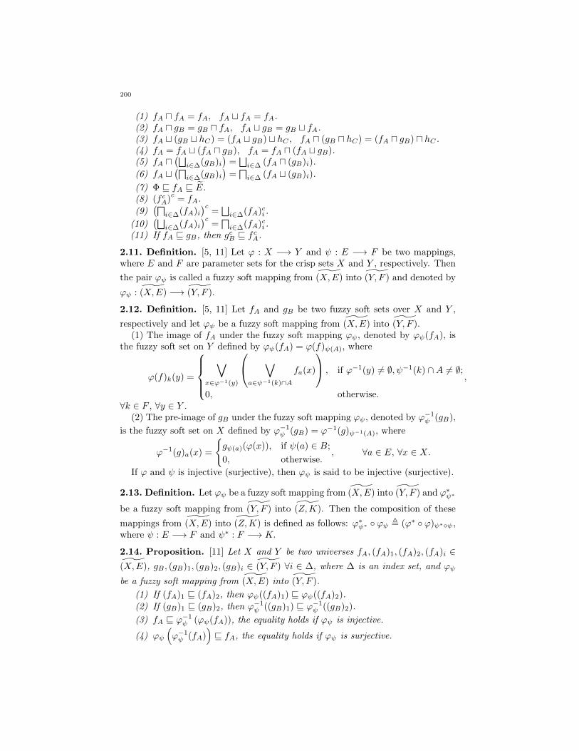
(1) fA u fA = fA, fA t fA = fA.(2) fA u gB = gB u fA, fA t gB = gB t fA.(3) fA t (gB t hC) = (fA t gB) t hC , fA u (gB u hC) = (fA u gB) u hC .(4) fA = fA t (fA u gB), fA = fA u (fA t gB).(5) fA u
(⊔i∈∆(gB)i
)=⊔i∈∆ (fA u (gB)i).
(6) fA t(d
i∈∆(gB)i)
=di∈∆ (fA t (gB)i).
(7) Φ v fA v E.(8) (f cA)
c= fA.
(9)(d
i∈∆(fA)i)c
=⊔i∈∆(fA)ci .
(10)(⊔
i∈∆(fA)i)c
=di∈∆(fA)ci .
(11) If fA v gB, then gcB v f cA.
2.11. Definition. [5, 11] Let ϕ : X −→ Y and ψ : E −→ F be two mappings,where E and F are parameter sets for the crisp sets X and Y , respectively. Then
the pair ϕψ is called a fuzzy soft mapping from (X,E) into (Y, F ) and denoted by
ϕψ : (X,E) −→ (Y, F ).
2.12. Definition. [5, 11] Let fA and gB be two fuzzy soft sets over X and Y ,
respectively and let ϕψ be a fuzzy soft mapping from (X,E) into (Y, F ).(1) The image of fA under the fuzzy soft mapping ϕψ, denoted by ϕψ(fA), is
the fuzzy soft set on Y defined by ϕψ(fA) = ϕ(f)ψ(A), where
ϕ(f)k(y) =
∨
x∈ϕ−1(y)
∨
a∈ψ−1(k)∩Afa(x)
, if ϕ−1(y) 6= ∅, ψ−1(k) ∩A 6= ∅;
0, otherwise.
,
∀k ∈ F , ∀y ∈ Y .(2) The pre-image of gB under the fuzzy soft mapping ϕψ, denoted by ϕ−1
ψ (gB),
is the fuzzy soft set on X defined by ϕ−1ψ (gB) = ϕ−1(g)ψ−1(A), where
ϕ−1(g)a(x) =
gψ(a)(ϕ(x)), if ψ(a) ∈ B;
0, otherwise., ∀a ∈ E, ∀x ∈ X.
If ϕ and ψ is injective (surjective), then ϕψ is said to be injective (surjective).
2.13. Definition. Let ϕψ be a fuzzy soft mapping from (X,E) into (Y, F ) and ϕ∗ψ∗
be a fuzzy soft mapping from (Y, F ) into (Z,K). Then the composition of these
mappings from (X,E) into (Z,K) is defined as follows: ϕ∗ψ∗ ϕψ , (ϕ∗ ϕ)ψ∗ψ,where ψ : E −→ F and ψ∗ : F −→ K.
2.14. Proposition. [11] Let X and Y be two universes fA, (fA)1, (fA)2, (fA)i ∈(X,E), gB , (gB)1, (gB)2, (gB)i ∈ (Y, F ) ∀i ∈ ∆, where ∆ is an index set, and ϕψ
be a fuzzy soft mapping from (X,E) into (Y, F ).
(1) If (fA)1 v (fA)2, then ϕψ((fA)1) v ϕψ((fA)2).
(2) If (gB)1 v (gB)2, then ϕ−1ψ ((gB)1) v ϕ−1
ψ ((gB)2).
(3) fA v ϕ−1ψ (ϕψ(fA)), the equality holds if ϕψ is injective.
(4) ϕψ
(ϕ−1ψ (fA)
)v fA, the equality holds if ϕψ is surjective.
200

(5) ϕψ(⊔
i∈∆(fA)i)
=⊔i∈∆ ϕψ((fA)i).
(6) ϕψ(d
i∈∆(fA)i)v d
i∈∆ ϕψ((fA)i), the equality holds if ϕψ is injective.
(7) ϕ−1ψ
(⊔i∈∆(gB)i
)=⊔i∈∆ ϕ−1
ψ ((gB)i).
(8) ϕ−1ψ
(di∈∆(gB)i
)=
di∈∆ ϕ−1
ψ ((gB)i).
(9) ϕ−1ψ (gcB) =
(ϕ−1ψ (gB)
)c.
(10) ϕ−1ψ
(EY
)= EX , ϕ−1
ψ (ΦY ) = ΦX .
(11) ϕψ
(EX
)= EY if ϕψ is surjective.
(12) ϕψ (ΦX) = ΦY .
2.15. Definition. (Cartesian product of two fuzzy soft sets) Let X1 and X2 be
nonempty crisp sets. fA ∈ ˜(X1, E1) and gB ∈ ˜(X2, E2). The cartesian productfA × gB of fA and gB is defined by (f × g)A×B , where, for each (e, f) ∈ E1 × E2,
(f × g)(e,f)(x, y) = fe(x) ∧ gf(y), for all (x, y) ∈ X × Y .According to this definition the fuzzy soft set (f × g)A×B is a fuzzy soft set on
X1 ×X2 and the universal parameter set is E1 × E2.
2.16. Definition. Let (fA)1×(fA)2 be a fuzzy soft set on X1×X2. The projectionmappings (pq)i, i ∈ 1, 2, are defined as follows:
(pq)i((fA)1 × (fA)2) = pi(f1 × f2)qi(A1×A2) = (fA)i where pi : X1 ×X2 −→ Xi
and qi : E1 × E2 −→ Ei are projection mappings in classical meaning.
3. Fuzzy soft topological spaces
To formulate our program and general ideas more precisely, recall first theconcept of fuzzy topological space, that is of a pair (X, τ) where X is a set andτ : IX −→ I is a mapping (satisfying some axioms) which assigns to every fuzzysubset of X the real number, which shows “to what extent” this set is open.According to this idea a fuzzy topology τ is a fuzzy set on IX . This approach haslead us to define fuzzy soft topology which is compatible to the fuzzy soft theory.By our definition, a fuzzy soft topology is a fuzzy soft set on the set of all fuzzy
soft sets (X,E) which denotes “to what extent” this set is open according to theparameter set.
3.1. Definition. A mapping τ : E −→ [0, 1](X,E) is called a fuzzy soft topologyon X if it satisfies the following conditions for each e ∈ E.
(O1) τe(Φ) = τe(E) = 1.
(O2) τe(fA u gB) ≥ τe(fA) ∧ τe(gB), ∀fA, gB ∈ (X,E).
(O3) τe(⊔i∈∆(fA)i) ≥
∧i∈∆ τe((fA)i),∀(fA)i ∈ (X,E), i ∈ ∆.
A fuzzy soft topology is called enriched if it provides that
(O1)′ τe(Eλ) = 1.Then the pair (X, τE) is called a fuzzy soft topological space. The value τe(fA)
is interpreted as the degree of openness of a fuzzy soft set fA with respect toparameter e ∈ E.
201
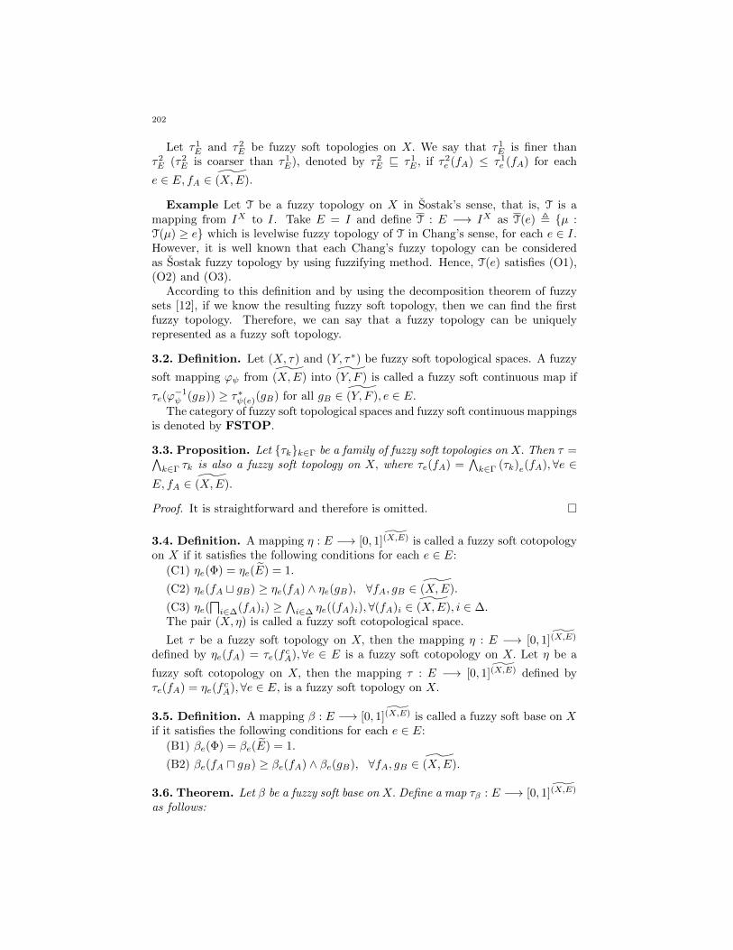
Let τ1E and τ2
E be fuzzy soft topologies on X. We say that τ1E is finer than
τ2E (τ2
E is coarser than τ1E), denoted by τ2
E v τ1E , if τ2
e (fA) ≤ τ1e (fA) for each
e ∈ E, fA ∈ (X,E).
Example Let T be a fuzzy topology on X in Sostak’s sense, that is, T is amapping from IX to I. Take E = I and define T : E −→ IX as T(e) , µ :T(µ) ≥ e which is levelwise fuzzy topology of T in Chang’s sense, for each e ∈ I.However, it is well known that each Chang’s fuzzy topology can be consideredas Sostak fuzzy topology by using fuzzifying method. Hence, T(e) satisfies (O1),(O2) and (O3).
According to this definition and by using the decomposition theorem of fuzzysets [12], if we know the resulting fuzzy soft topology, then we can find the firstfuzzy topology. Therefore, we can say that a fuzzy topology can be uniquelyrepresented as a fuzzy soft topology.
3.2. Definition. Let (X, τ) and (Y, τ∗) be fuzzy soft topological spaces. A fuzzy
soft mapping ϕψ from (X,E) into (Y, F ) is called a fuzzy soft continuous map if
τe(ϕ−1ψ (gB)) ≥ τ∗ψ(e)(gB) for all gB ∈ (Y, F ), e ∈ E.
The category of fuzzy soft topological spaces and fuzzy soft continuous mappingsis denoted by FSTOP.
3.3. Proposition. Let τkk∈Γ be a family of fuzzy soft topologies on X. Then τ =∧k∈Γ τk is also a fuzzy soft topology on X, where τe(fA) =
∧k∈Γ (τk)e(fA),∀e ∈
E, fA ∈ (X,E).
Proof. It is straightforward and therefore is omitted.
3.4. Definition. A mapping η : E −→ [0, 1](X,E) is called a fuzzy soft cotopologyon X if it satisfies the following conditions for each e ∈ E:
(C1) ηe(Φ) = ηe(E) = 1.
(C2) ηe(fA t gB) ≥ ηe(fA) ∧ ηe(gB), ∀fA, gB ∈ (X,E).
(C3) ηe(di∈∆(fA)i) ≥
∧i∈∆ ηe((fA)i),∀(fA)i ∈ (X,E), i ∈ ∆.
The pair (X, η) is called a fuzzy soft cotopological space.
Let τ be a fuzzy soft topology on X, then the mapping η : E −→ [0, 1](X,E)
defined by ηe(fA) = τe(fcA),∀e ∈ E is a fuzzy soft cotopology on X. Let η be a
fuzzy soft cotopology on X, then the mapping τ : E −→ [0, 1](X,E) defined byτe(fA) = ηe(f
cA),∀e ∈ E, is a fuzzy soft topology on X.
3.5. Definition. A mapping β : E −→ [0, 1](X,E) is called a fuzzy soft base on Xif it satisfies the following conditions for each e ∈ E:
(B1) βe(Φ) = βe(E) = 1.
(B2) βe(fA u gB) ≥ βe(fA) ∧ βe(gB), ∀fA, gB ∈ (X,E).
3.6. Theorem. Let β be a fuzzy soft base on X. Define a map τβ : E −→ [0, 1](X,E)
as follows:
202
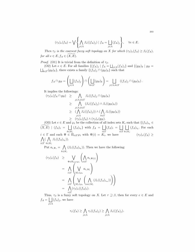
(τβ)e(fA) =∨∧
j∈Λ
βe((fA)j) | fA =⊔
j∈Λ
(fA)j
, ∀e ∈ E.
Then τβ is the coarsest fuzzy soft topology on X for which (τβ)e(fA) ≥ βe(fA),
for all e ∈ E, fA ∈ (X,E).
Proof. (O1) It is trivial from the definition of τβ .(O2) Let e ∈ E. For all families (fA)j | fA =
⊔j∈Λ(fA)j and (gB)k | gB =⊔
k∈Γ(gB)k, there exists a family (fA)j u (gB)k such that
fA u gB =
⊔
j∈Λ
(fA)j
u
(⊔
k∈Γ
(gB)k
)=
⊔
j∈Λ,k∈Γ
((fA)j u (gB)k) .
It implies the followings:
(τβ)e(fA u gB) ≥∧
j∈Λ,k∈Γ
βe((fA)j u (gB)k)
≥∧
j∈Λ,k∈Γ
(βe((fA)j) ∧ βe((gB)k))
≥ (∧
j∈Λ
βe((fA)j)) ∧ (∧
k∈Γ
βe((gB)k))
≥ (τβ)e(fA) ∧ (τβ)e(gB).(O3) Let e ∈ E and ℘i be the collection of all index sets Ki such that (fA)ik ∈
(X,E) | (fA)i =⊔
k∈Ki
(fA)ik with fA =⊔
i∈Γ
(fA)i =⊔
i∈Γ
⊔
k∈Ki
(fA)ik . For each
i ∈ Γ and each Ψ ∈ Πi∈Γ℘i with Ψ(i) = Ki, we have (τβ)e(fA) ≥∧
i∈Γ
(∧
k∈Ki
βe((fA)ik)).
Put ai,Ψi =∧
k∈Ki
(βe((fA)ik)). Then we have the following:
(τβ)e(fA) ≥∨
Ψ∈Πi∈Γ℘i
(∧
i∈Γ
ai,Ψ(i)
)
=∧
i∈Γ
∨
Mi∈℘i
ai,Mi
=∧
i∈Γ
∨
Mi∈℘i
( ∧
m∈Mi
(βe((fA)im))
)
=∧
i∈Γ
(τβ)e((fA)i).
Thus, τβ is a fuzzy soft topology on X. Let τ w β, then for every e ∈ E and
fA =⊔
j∈Λ
(fA)j , we have
τe(fA) ≥∧
j∈Λ
τe((fA)j) ≥∧
j∈Λ
βe((fA)j).
203
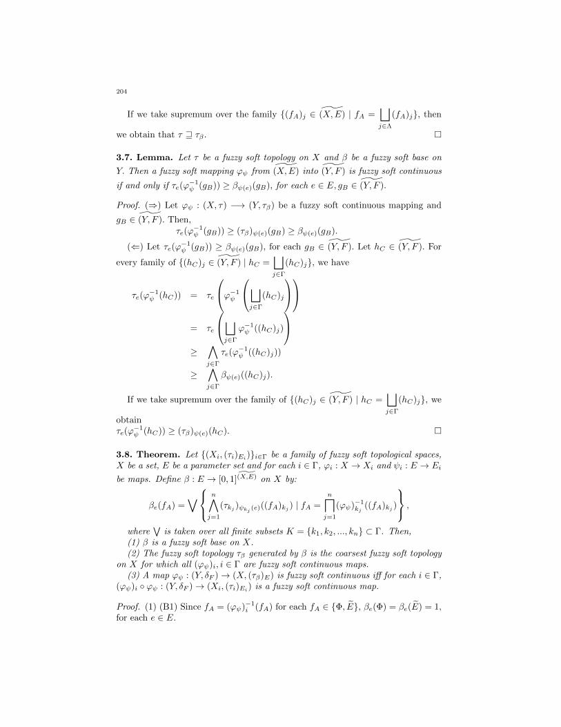
If we take supremum over the family (fA)j ∈ (X,E) | fA =⊔
j∈Λ
(fA)j, then
we obtain that τ w τβ .
3.7. Lemma. Let τ be a fuzzy soft topology on X and β be a fuzzy soft base on
Y. Then a fuzzy soft mapping ϕψ from (X,E) into (Y, F ) is fuzzy soft continuous
if and only if τe(ϕ−1ψ (gB)) ≥ βψ(e)(gB), for each e ∈ E, gB ∈ (Y, F ).
Proof. (⇒) Let ϕψ : (X, τ) −→ (Y, τβ) be a fuzzy soft continuous mapping and
gB ∈ (Y, F ). Then,τe(ϕ
−1ψ (gB)) ≥ (τβ)ψ(e)(gB) ≥ βψ(e)(gB).
(⇐) Let τe(ϕ−1ψ (gB)) ≥ βψ(e)(gB), for each gB ∈ (Y, F ). Let hC ∈ (Y, F ). For
every family of (hC)j ∈ (Y, F ) | hC =⊔
j∈Γ
(hC)j, we have
τe(ϕ−1ψ (hC)) = τe
ϕ−1
ψ
⊔
j∈Γ
(hC)j
= τe
⊔
j∈Γ
ϕ−1ψ ((hC)j)
≥∧
j∈Γ
τe(ϕ−1ψ ((hC)j))
≥∧
j∈Γ
βψ(e)((hC)j).
If we take supremum over the family of (hC)j ∈ (Y, F ) | hC =⊔
j∈Γ
(hC)j, we
obtainτe(ϕ
−1ψ (hC)) ≥ (τβ)ψ(e)(hC).
3.8. Theorem. Let (Xi, (τi)Ei)i∈Γ be a family of fuzzy soft topological spaces,
X be a set, E be a parameter set and for each i ∈ Γ, ϕi : X → Xi and ψi : E → Ei
be maps. Define β : E → [0, 1](X,E) on X by:
βe(fA) =∨
n∧
j=1
(τkj )ψkj(e)((fA)kj ) | fA =
nl
j=1
(ϕψ)−1kj
((fA)kj )
,
where∨
is taken over all finite subsets K = k1, k2, ..., kn ⊂ Γ. Then,(1) β is a fuzzy soft base on X.(2) The fuzzy soft topology τβ generated by β is the coarsest fuzzy soft topology
on X for which all (ϕψ)i, i ∈ Γ are fuzzy soft continuous maps.(3) A map ϕψ : (Y, δF )→ (X, (τβ)E) is fuzzy soft continuous iff for each i ∈ Γ,
(ϕψ)i ϕψ : (Y, δF )→ (Xi, (τi)Ei) is a fuzzy soft continuous map.
Proof. (1) (B1) Since fA = (ϕψ)−1i (fA) for each fA ∈ Φ, E, βe(Φ) = βe(E) = 1,
for each e ∈ E.
204

(B2) For all finite subsets K = k1, k2, ..., kn and J = j1, j2, ..., jm of Γ such
that fA =
nl
i=1
(ϕψ)−1ki
((fA)ki) and gB =
ml
i=1
(ϕψ)−1ji
((gB)ji), we have fA u gB =
(nl
i=1
(ϕψ)−1ki
((fA)ki)
)u(
ml
i=1
(ϕψ)−1ji
((gB)ji)
).
Furthermore, we have for each k ∈ K ∩ J,
(ϕψ)−1k ((fA)k) u (ϕψ)−1
k ((gB)k) = (ϕψ)−1k ((fA)k u (gB)k).
Put fA u gB =l
mi∈K∪J(ϕψ)−1
mi((hC)mi
) where
(hC)mi=
(fA)mi, if mi ∈ K − (K ∩ J);
(gB)mi , if mi ∈ J − (K ∩ J);
(fA)mi u (gB)mi , if mi ∈ (K ∩ J).So we haveβe((fA) u (gB)) ≥
∧
j∈K∪J(τj)ψj(e)((hC)j)
≥(
n∧
i=1
(τki)ψki(e)((fA)ki)
)∧(
m∧
i=1
(τji)ψji(e)((gB)ji)
).
If we take supremum over the families fA =nl
i=1
(ϕψ)−1ki
((fA)ki) and gB =
ml
i=1
(ϕψ)−1ji
((gB)ji), then we have,
βe(fA u gB) ≥ βe(fA) ∧ βe(gB),∀e ∈ E.
(2) For each (fA)i ∈ ˜(Xi, Ei), one family (ϕψ)−1i ((fA)i) and i ∈ Γ, we have
(τβ)e((ϕψ)−1i ((fA)i)) ≥ βe((ϕψ)−1
i ((fA)i)) ≥ (τi)ψi(e)((fA)i), for each e ∈ E.
Therefore, for all i ∈ Γ, (ϕψ)i : (X, (τβ)E) −→ (Xi, (τi)Ei) is fuzzy soft contin-
uous.Let (ϕψ)i : (X, ζE) −→ (Xi, (τi)Ei
) be fuzzy soft continuous, that is, for each
i ∈ Γ and (fA)i ∈ ˜(Xi, Ei), ζe((ϕψ)−1i ((fA)i)) ≥ (τi)ψi(e)((fA)i).
For all finite subsets K = k1, ..., kn of Γ such that fA =
nl
i=1
(ϕψ)−1ki
((fA)ki)
we have
ζe(fA) ≥n∧
i=1
ζe((ϕψ)−1ki
((fA)ki)) ≥n∧
i=1
(τki)ψki(e)((fA)ki).
It implies ζe(fA) ≥ βe(fA), for all e ∈ E, fA ∈ (X,E). By Theorem 3.6, ζ w τβ .(3) (⇒) Let ϕψ : (Y, δF )→ (X, (τβ)E) be fuzzy soft continuous. For each i ∈ Γ
and (fA)i ∈ ˜(Xi, Ei) we have
205

δf((ϕi ϕ)−1ψiψ((fA)i)) = δf(ϕ
−1ψ ((ϕψ)−1
i ((fA)i))) ≥ (τβ)ψ(f)((ϕψ)−1i ((fA)i)) ≥
(τi)(ψiψ)(f)((fA)i).
Hence, (ϕi ϕ)ψiψ : (Y, δF )→ (Xi, (τi)Ei) is fuzzy soft continuous.
(⇐) For all finite subsetsK = k1, ..., kn of Γ such that fA =nl
i=1
(ϕψ)−1ki
((fA)ki),
since(ϕkiϕ)ψki
ψ : (Y, δF )→ (Xki , (τki)Eki) is fuzzy soft continuous, δf(ϕ
−1ψ ((ϕψ)−1
ki((fA)ki))) ≥
(τki)(ψiψ)(f)((fA)ki),∀ f ∈ F.Hence we have
δf(ϕ−1ψ (fA)) = δf(ϕ
−1ψ (
nl
i=1
(ϕψ)−1ki
((fA)ki)))
= δf(
nl
i=1
(ϕ−1ψ ((ϕψ)−1
ki(((fA)ki)))))
≥n∧
i=1
δf(ϕ−1ψ ((ϕψ)−1
ki(((fA)ki))))
≥n∧
i=1
(τki)(ψkiψ)(f)((fA)ki).
This inequality implies that δf(ϕ−1ψ (fA)) ≥ βψ(f)(fA) for each fA ∈ (X,E), f ∈
F.By Lemma 3.7, ϕψ : (Y, δF )→ (X, (τβ)E) is fuzzy soft continuous.Let (Xi, (τi)Ei)i∈Γ be a family of fuzzy soft topological spaces, X be a set,
E be a parameter set and for each i ∈ Γ, ϕi : X → Xi and ψi : E → Ei be maps.The initial fuzzy soft topology τβ on X is the coarsest fuzzy soft topology on Xfor which all (ϕψ)i, i ∈ Γ are fuzzy soft continuous maps.
3.9. Definition. [1] A category C is called a topological category over SET withrespect to the usual forgetful functor from C to SET if it satisfies the followingconditions:
(TC1) Existence of initial structures: For any X, any class J, and any family((Xj , ξj))j∈J of C-object and any family (fj : X −→ Xj)j∈J of maps, there existsa unique C-structure ξ on X which is initial with respect to the source (fj : X −→(Xj , ξj))j∈J , this means that for a C-object (Y, η), a map g : (Y, η) −→ (X, ξ) is aC-morphism if and only if for all j ∈ J, fj g : (Y, η) −→ (Xj , ξj) is a C-morphism.
(TC2) Fibre smallness: For any set X, the C-fibre of X, i.e., the class of allC-structure on X, which we denote C(X), is a set.
3.10. Theorem. The category FSTOP is a topological category over SET withrespect to the forgetful functor V : FSTOP−→ SET which is defined by V (X, τE) =X and V (ϕψ) = ϕ.
Proof. The proof is straightforward and follows from Theorem 3.8.
3.11. Definition. Let (Xi, (τi)Ei)i∈Γ be a family of fuzzy soft topological
spaces, for each i ∈ Γ, Ei be parameter sets, X = Πi∈ΓXi and E = Πi∈ΓEi.Let pi : X −→ Xi and qi : E −→ Ei be projection maps, for all i ∈ Γ. The product
206

of fuzzy soft topologies (X, τE) with respect to parameter set E is the coarsestfuzzy soft topology on X for which all (pq)i, i ∈ Γ, are fuzzy soft continuous maps.
4. Conclusion
In this paper, we have considered the topological structure of fuzzy soft settheory. We have given the definition of fuzzy soft topology τ which is a mapping
from the parameter set E to [0, 1](X,E) which satisfy the three certain conditions.Since the value of a fuzzy soft set fA under the mapping τe gives us the degreeof openness of the fuzzy soft set with respect to the parameter e ∈ E, τe canbe thought of as a fuzzy soft topology in the sense of Sostak. In this sense, wehave introduced fuzzy soft cotopology and given the relations between fuzzy softtopology and fuzzy soft cotopology. Then we have defined fuzzy soft base and byusing a fuzzy soft base we have obtained a fuzzy soft topology on the same set.Also, we have introduced an initial fuzzy soft topology and then we have giventhe definition of product fuzzy soft topology. Further, we have proved that thecategory of fuzzy soft topological spaces FSTOP is a topological category overSET with respect to the forgetful functor.
References
[1] J. Adamek, H. Herrlich, G. E. Strecker, Abstract and Concrete Categories, Wiley, New York,
1990.[2] B. Ahmad, A. Kharal, On Fuzzy Soft Sets, Advances in Fuzzy Systems, Volume 2009, Article
ID 586507
[3] H. Aktas, N. Cagman, Soft sets and soft groups, Information Sciences 177 (13) (2007) 2726-2735.
[4] K. Atanassov, Intuitionistic Fuzzy Sets, Fuzzy Sets and Systems 64 (2) (1986) 87-96.
[5] A. Aygunoglu, H. Aygun, Introduction to fuzzy soft groups, Computers and Mathematicswith Applications 58 (2009) 1279-1286
[6] F. Feng, Y. B. Jun, X. Zhao, Soft semirings, Computers and Mathematics with Applications
56 (10) (2008) 2621-2628.[7] Y. B. Jun, Soft BCK/BCI algebras, Computers and Mathematics with Applications 56 (5)
(2008) 1408-1413.
[8] Y. B. Jun, C. H. Park, Applications of soft sets in ideal theory of BCK/BCI algebras,Information Sciences 178 (11) (2008) 2466-2475.
[9] Y. B. Jun, K. J. Lee, C. H. Park, Soft set theory applied to ideals in d-algebras, Computers
and Mathematics with Applications 57 (3) (2009) 367-378.[10] Y. B. Jun, K. J. Lee, J. Zhan, Soft p-ideals of soft BCI-algebras, Computers and Mathe-
matics with Applications 58 (10) (2009) 2060-2068.[11] A. Kharal, B. Ahmad, Mappings on Fuzzy Soft Classes, Advances in Fuzzy Systems, Volume
2009, Article ID 407890
[12] G.J. Klir, B. Yuan, Fuzzy sets and fuzzy logic, Theory and Applications, Prentice-Hall Inc.,New Jersey, 1995.
[13] P.K. Maji, R. Biswas, A.R. Roy, Fuzzy soft sets, Journal of fuzzy Mathematics, 9(3) (2001)
589-602.[14] P. K. Maji, A. R. Roy and R. Biswas, An application of soft sets in a decision making
problem, Computers and Mathematics with Applications 44 (8-9) (2002) 1077-1083.
[15] D. Molodtsov, Soft set theory-First results, Computers Mathematics with Appl. 37 (4/5)(1999) 19-31.
[16] Z. Pawlak, Rough Sets, International Journal of Information and Computer Science 11 (1982)
341-356.
207

[17] D. Pei, D. Miao, From soft sets to information systems, Granular Computing, 2005 IEEE
International Conference on (2) (2005) 617-621.
[18] A.R. Roy, P.K. Maji, A fuzzy soft set theoretic approach to decision making problems,Journal of Computational and Applied Mathematics, 203 (2007) 412-418.
[19] A. P. Sostak, On a fuzzy topological structure, Suppl. Rend. Circ. Matem. Palermo, Ser II11 (1985) 89-103.
[20] Q. M. Sun, Z. L. Zhang, J. Liu, Soft sets and soft modules in: G. Wang, T. Li, J. W.
Grzymala-Busse, D. Miao, A. Skowron, Y. Yao (Eds.) Proceedings of the Third Interna-tional Conference on Rough Sets and Knowledge Technology, RSKT 2008, in: Lecture Notes
in Computer Science, vol. 5009, Springer (2008) 403-409.
[21] L. A. Zadeh, Fuzzy Sets, Information and Control 8 (1965) 338-353.
208

Hacettepe Journal of Mathematics and StatisticsVolume 43 (2) (2014), 209 – 225
Convergence to common fixed points ofmulti-step iteration process for generalized
asymptotically quasi-nonexpansive mappings inconvex metric spaces
G. S. Saluja∗
Abstract
In this paper, we study strong convergence of multi-step iterationswith errors for a finite family of generalized asymptotically quasi-nonexpansive mappings in the framework of convex metric spaces. Thenew iteration scheme includes modified Mann and Ishikawa iterationswith errors, the three-step iteration scheme of Xu and Noor as specialcases in Banach spaces. Our results extend and generalize many knownresults from the current literature.
Keywords: Generalized asymptotically quasi-nonexpansive mapping, multi-stepiterations with errors, common fixed point, strong convergence, convex metric
2000 AMS Classification: 47H09, 47H10.
1. Introduction and Preliminaries
Let T be a self map on a nonempty subset C of a metric space (X, d). Denotethe set of fixed points of T by F (T ) = x ∈ C : T (x) = x. We say that T is:
(1) nonexpansive if
d(Tx, Ty) ≤ d(x, y)(1.1)
for all x, y ∈ C;
(2) quasi-nonexpansive if F (T ) 6= ∅ and
d(Tx, p) ≤ d(x, p)(1.2)
for all x ∈ C and p ∈ F (T );
∗Department of Mathematics and Information Technology, Govt. Nagarjuna P.G. Col-
lege of Science, Raipur - 492010 (C.G.), India, Email: saluja [email protected],

(3) asymptotically nonexpansive [5] if there exists a sequence rn ⊂ [0,∞)with limn→∞ rn = 0 such that
d(Tnx, Tny) ≤ (1 + rn)d(x, y),(1.3)
for all x, y ∈ C and n ≥ 1;
(4) asymptotically quasi-nonexpansive if F (T ) 6= ∅ and there exists a sequencern ⊂ [0,∞) with limn→∞ rn = 0 such that
d(Tnx, p) ≤ (1 + rn)d(x, p),(1.4)
for all x ∈ C, p ∈ F (T ) and n ≥ 1;
(5) generalized asymptotically quasi-nonexpansive [6] if F (T ) 6= ∅ and thereexist two sequences of real numbers rn, sn ⊂ [0,∞) with limn→∞ rn = 0 =limn→∞ sn such that
d(Tnx, p) ≤ (1 + rn)d(x, p) + sn,(1.5)
for all x ∈ C, p ∈ F (T ) and n ≥ 1;
(6) uniformly L-Lipschitzian if there exists a constant L > 0 such that
d(Tnx, Tny) ≤ L d(x, y),(1.6)
for all x, y ∈ C and n ≥ 1;
(7) semi-compact if for any bounded sequence xn in C with d(xn, Txn)→ 0as n→∞, there is a convergent subsequence of xn.
Let xn be a sequence in a metric space (X, d), and let C be a subset of X.We say that xn is:
(8) of monotone type [22] with respect to C if for each p ∈ C, there exist twosequences an and bn of nonnegative real numbers such that
∑∞n=1 an < ∞,∑∞
n=1 bn <∞ and
d(xn+1, p) ≤ (1 + an)d(xn, p) + bn. (∗)
1.1. Remark. (1) It is clear that the nonexpansive mappings with the nonemptyfixed point set F (T ) are quasi-nonexpansive.
(2) The linear quasi-nonexpansive mappings are nonexpansive, but it is eas-ily seen that there exist nonlinear continuous quasi-nonexpansive mappings whichare not nonexpansive; for example, define T (x) = (x/2)sin(1/x) for all x 6= 0 and
210

T (0) = 0 in R.
(3) It is obvious that if T is nonexpansive, then it is asymptotically nonexpan-sive with the constant sequence 1.
(4) If T is asymptotically nonexpansive, then it is uniformly Lipschitzian withthe uniform Lipschitz constant L = sup1 + rn : n ≥ 1. However, the converse ofthis claim is not true.
(5) If in definition (5), sn = 0 for all n ≥ 1, then T becomes asymptoti-cally quasi-nonexpansive, and hence the class of generalized asymptotically quasi-nonexpansive maps includes the class of asymptotically quasi-nonexpansive maps.
In 1991, Schu [16, 17] introduced the following iterative scheme: let X be anormed linear space, let C be a nonempty convex subset of X, and let T : C → Cbe a given mapping. Then, for arbitrary x1 ∈ C, the modified Ishikawa iterativescheme xn is defined by
yn = (1− βn)xn + βnTnxn
xn+1 = (1− αn)xn + αnTnyn, n ≥ 1,(1.7)
where αn and βn are some suitable sequences [0, 1]. With X, C, αn, andx1 as above, the modified Mann iterative scheme xn is defined by
x1 ∈ C,
xn+1 = (1− αn)xn + αnTnxn, n ≥ 1.(1.8)
In 1998, Xu [21] introduced the following iterative scheme: let X be a normedlinear space, let C be a nonempty convex subset of X, and let T : C → C be agiven mapping. Then, for arbitrary x1 ∈ C, the Ishikawa iterative scheme xnwith errors is defined by
yn = anxn + bnTxn + cnvn
xn+1 = anxn + bnTyn + cnun, n ≥ 1,(1.9)
where un, vn are bounded sequences in C and an, bn, cn, an, bn,cn are sequences [0, 1] with an + bn + cn = an + bn + cn = 1. With X, C, un,an, bn, cn, and x1 as above, the Mann iterative scheme xn with errors isdefined by
x1 ∈ C,
xn+1 = anxn + bnTxn + cnun, n ≥ 1.(1.10)
Based on the iterative scheme with errors introduced by Xu [21], the follow-ing iteration schemes have been used and studied by several authors (see [1, 3, 12]).
211

Let X be a normed linear space, let C be a nonempty convex subset of X, andlet T : C → C be a given mapping. Then, for arbitrary x1 ∈ C, the modifiedIshikawa iteration scheme xn with errors is defined by
yn = anxn + bnTnxn + cnvn
xn+1 = anxn + bnTnyn + cnun, n ≥ 1,(1.11)
where un, vn are bounded sequences in C and an, bn, cn, an, bn,cn are sequences [0, 1] with an + bn + cn = an + bn + cn = 1. With X, C, un,an, bn, cn, and x1 as above, the modified Mann iteration scheme xn witherrors is defined by
x1 ∈ C,xn+1 = anxn + bnT
nxn + cnun, n ≥ 1.(1.12)
Recently, Imnang and Suantai [6] studied multi-step Noor iterations with errorsfor a finite family of generalized asymptotically quasi-nonexpansive mappings andestablished some strong convergence theorems in the framework of uniformly con-vex Banach spaces. The scheme of [6] is as follows: Let Ti : C → C (i = 1, 2, . . . , k)
be mappings and F =⋂ki=1 F (Ti). For a given x1 ∈ C, and a fixed k ∈ N (N de-
note the set of all positive integers), compute the iterative sequences xn andyin by
xn+1 = ykn = αknTnk y(k−1)n + βknxn + γknukn,
y(r−1)n = α(k−1)nTnk−1y(k−2)n + β(k−1)nxn + γ(k−1)nu(k−1)n,
...
y3n = α3nTn3 y2n + β3nxn + γ3nu3n,
y2n = α2nTn2 y1n + β2nxn + γ2nu2n,
y1n = α1nTn1 y0n + β1nxn + γ1nu1n, n ≥ 1.(1.13)
where y0n = xn and u1n, u2n, . . . , ukn are bounded sequences in C withαin, βin, and γin are appropriate real sequences in [0, 1] such that αin +βin + γin = 1 for all i = 1, 2, . . . , k and all n. This iteration scheme includes themodified Mann iteration scheme (1.12), the modified Ishikawa iteration scheme(1.11) and extends the three-step iteration by Xu and Noor [20].
One of the most interesting aspects of metric fixed point theory is to extend alinear version of a known result to the nonlinear case in metric spaces. To achievethis, Takahashi [18] introduced a convex structure in a metric space (X, d) andthe properties of the space.
1.2. Definition. Let (X, d) be a metric space and I = [0, 1]. A mapping W : X3×I3 → X is said to be a convex structure on X if it satisfies the following condition:
d(u,W (x, y, z;α, β, γ)) ≤ αd(u, x) + βd(u, y) + γd(u, z),
212

for any u, x, y, z ∈ X and for any α, β, γ ∈ I with α+ β + γ = 1.
If (X, d) is a metric space with a convex structure W , then (X, d) is called aconvex metric space and denotes it by (X, d,W ).
1.3. Remark. It is easy to prove that every linear normed space is a convexmetric space with a convex structure W (x, y, z;α, β, γ) = αx + βy + γz, for allx, y, z ∈ X and α, β, γ ∈ I with α+β+γ = 1. But there exist some convex metricspaces which can not be embedded into any linear normed spaces (see, Takahashi[18]).
1.4. Example. Let X = (x1, x2, x3) ∈ R3 : x1 > 0, x2 > 0, x3 > 0. Forx = (x1, x2, x3), y = (y1, y2, y3) ∈ X and α, β, γ ∈ I with α+ β + γ = 1, we definea mapping W : X3 × I3 → X by
W (x, y, z;α, β, γ) = (αx1 + βy1 + γz1, αx2 + βy2 + γz2, αx3 + βy3 + γz3)
and define a metric d : X ×X → [0,∞) by
d(x, y) = |x1y1 + x2y2 + x3y3|.
Then we can show that (X, d,W ) is a convex metric space, but it is not a normedspace.
Denote the indexing set 1, 2, . . . , k by I. We now translate the scheme (1.13)from the normed space setting to the more general setup of convex metric spaceas follows:
x1 ∈ C, xn+1 = Un(k)xn, n ≥ 1,(1.14)
where
Un(0) = I, the identity map,
Un(1)x = W (Tn1 Un(0)x, x, un(1); αn(1), βn(1), γn(1)),
Un(2)x = W (Tn2 Un(1)x, x, un(2); αn(2), βn(2), γn(2)),
...
Un(k−1)x = W (Tnk−1Un(k−2)x, x, un(k−1); αn(k−1), βn(k−1), γn(k−1)),
Un(k)x = W (Tnk Un(k−1)x, x, un(k); αn(k), βn(k), γn(k)), n ≥ 1,
where un(1), un(2), . . . , un(k) are bounded sequences in C with αn(i), βn(i),and γn(i) are appropriate real sequences in [0, 1] such that αn(i)+βn(i)+γn(i) = 1for all i ∈ I and all n.
213

In a convex metric space, the scheme (1.14) provides analogues of:
(i) the scheme (1.12) if k = 1 and T1 = T ;
(ii) the scheme (1.11) if k = 2 and T1 = T2 = T .
This scheme becomes the scheme (1.13) if we choose a special convex metricspace, namely, a normed space.
In this paper, we establish strong convergence theorem for the iteration scheme(1.14) to converge to common fixed point of a finite family of generalized asymp-totically quasi-nonexpansive mappings in the framework of convex metric spaces.Our result extends and as well as refines the corresponding results of [2], [4], [6]-[17], [20] and many others.
We need the following useful lemma to prove our convergence results.
1.5. Lemma. (see [19]) Let pn, qn, rn be three sequences of nonnegativereal numbers satisfying the following conditions:
pn+1 ≤ (1 + qn)pn + rn, n ≥ 0,∞∑
n=0
qn <∞,∞∑
n=0
rn <∞.
Then
(1) limn→∞ pn exists.
(2) In addition, if lim infn→∞ pn = 0, then limn→∞ pn = 0.
2. Main Results
In this section, we prove strong convergence theorems of multi-step iterationscheme (1.14) for a finite family of generalized asymptotically quasi-nonexpansivemappings in convex metric spaces.
2.1. Lemma. Let (X, d) be a complete convex metric space, and let C be anonempty closed convex subset of X. Let Ti : i ∈ I be a finite family of general-ized asymptotically quasi-nonexpansive self-maps on C with sequences rn(i), sn(i) ⊂[0,∞) for each i ∈ I, respectively, such that
∑∞n=1 rn(i) <∞ and
∑∞n=1 sn(i) <∞.
Assume that F = ∩ki=1F (Ti) is a nonempty set. Let xn be the multi-step itera-tion scheme defined by (1.14) with
∑∞n=1 γn(i) <∞ for each i ∈ I. Then
(i)
d(xn+1, p) ≤ (1 +Bn(k))d(xn, p) +An(k),
with∑∞n=1Bn(k) <∞ and
∑∞n=1An(k) <∞.
214

(ii)
d(xn+m, p) ≤ Qd(xn, p) +Q
n+m−1∑
j=n
Aj(k),
for m ≥ 1, n ≥ 1, p ∈ F and for some Q > 0.
Proof. (i) For any p ∈ F , from (1.14), we have
d(Un(1)xn, p) = d(W (Tn1 xn, xn, un(1); αn(1), βn(1), γn(1)), p)
≤ αn(1)d(Tn1 xn, p) + βn(1)d(xn, p) + γn(1)d(un(1), p)
≤ αn(1)[(1 + rn(1))d(xn, p) + sn(1)] + βn(1)d(xn, p) + γn(1)d(un(1), p)
≤ [αn(1) + βn(1)](1 + rn(1))d(xn, p) + αn(1)sn(1) + γn(1)d(un(1), p)
= [1− γn(1)](1 + rn(1))d(xn, p) +An(1)
≤ (1 + rn(1))d(xn, p) +An(1),(2.1)
where An(1) = αn(1)sn(1) + γn(1)d(un(1), p), since by assumption∑∞n=1 sn(1) < ∞
and∑∞n=1 γn(1) <∞, it follows that
∑∞n=1An(1) <∞.
Again from (1.14) and using (2.1), we have
d(Un(2)xn, p) = d(W (Tn2 Un(1)xn, xn, un(2); αn(2), βn(2), γn(2)), p)
≤ αn(2)d(Tn2 Un(1)xn, p) + βn(2)d(xn, p) + γn(2)d(un(2), p)
≤ αn(2)[(1 + rn(2))d(Un(1)xn, p) + sn(2)] + βn(2)d(xn, p) + γn(2)d(un(2), p)
≤ αn(2)(1 + rn(2))[(1 + rn(1))d(xn, p) +An(1)] + αn(2)sn(2) + βn(2)d(xn, p)
+γn(2)d(un(2), p)
≤ [αn(2) + βn(2)](1 + rn(1))(1 + rn(2))d(xn, p) + αn(2)(1 + rn(2))An(1)
+αn(2)sn(2) + βn(2)d(xn, p) + γn(2)d(un(2), p)
= [1− γn(2)](1 + rn(1) + rn(2) + rn(1)rn(2))d(xn, p) + αn(2)(1 + rn(2))An(1)
+αn(2)sn(2) + γn(2)d(un(2), p)
≤ (1 +Bn(2))d(xn, p) +An(2),(2.2)
where Bn(2) = rn(1) + rn(2) + rn(1)rn(2) and An(2) = αn(2)(1 + rn(2))An(1) +
αn(2)sn(2) + γn(2)d(un(2), p), since by assumptions∑∞n=1 rn(1) <∞,
∑∞n=1 rn(2)
< ∞,∑∞n=1 sn(2) < ∞,
∑∞n=1An(1) < ∞ and
∑∞n=1 γn(2) < ∞, it follows that∑∞
n=1Bn(2) <∞ and∑∞n=1An(2) <∞.
215

Further using (1.14) and (2.2), we have
d(Un(3)xn, p) = d(W (Tn3 Un(2)xn, xn, un(3); αn(3), βn(3), γn(3)), p)
≤ αn(3)d(Tn3 Un(2)xn, p) + βn(3)d(xn, p) + γn(3)d(un(3), p)
≤ αn(3)[(1 + rn(3))d(Un(2)xn, p) + sn(3)] + βn(3)d(xn, p) + γn(3)d(un(3), p)
≤ αn(3)(1 + rn(3))[(1 +Bn(2))d(xn, p) +An(2)] + αn(3)sn(3) + βn(3)d(xn, p)
+γn(3)d(un(3), p)
≤ [αn(3) + βn(3)](1 + rn(3))(1 +Bn(2))d(xn, p) + αn(3)(1 + rn(3))An(2)
+αn(3)sn(3) + βn(3)d(xn, p) + γn(3)d(un(3), p)
= [1− γn(3)](1 + rn(3) +Bn(2) + rn(3)Bn(2))d(xn, p) + αn(3)(1 + rn(3))An(2)
+αn(3)sn(3) + γn(3)d(un(3), p)
≤ (1 +Bn(3))d(xn, p) +An(3),(2.3)
where Bn(3) = rn(3) + Bn(2) + rn(3)Bn(2) and An(3) = αn(3)(1 + rn(3))An(2) +
αn(3)sn(3) + γn(3)d(un(3), p), since by assumptions∑∞n=1 rn(3) <∞,
∑∞n=1Bn(2)
< ∞,∑∞n=1 sn(3) < ∞,
∑∞n=1An(2) < ∞ and
∑∞n=1 γn(3) < ∞, it follows that∑∞
n=1Bn(3) <∞ and∑∞n=1An(3) <∞. Continuing in this process, we get
d(xn+1, p) ≤ (1 +Bn(k))d(xn, p) +An(k),(2.4)
where Bn(k) = rn(k)+Bn(k−1)+rn(k)Bn(k−1) and An(k) = αn(k)(1+rn(k))An(k−1)+
αn(k)sn(k) + γn(k)d(un(k), p) with∑∞n=1Bn(k) <∞ and
∑∞n=1An(k) <∞.
The conclusion (i) holds.
(ii) Note that when x > 0, 1 + x ≤ ex. It follows from conclusion (i) that form ≥ 1, n ≥ 1 and p ∈ F , we have
216
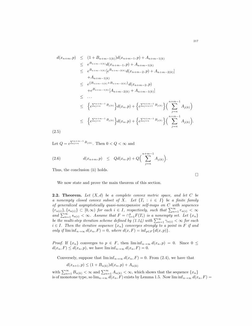
d(xn+m, p) ≤ (1 +Bn+m−1(k))d(xn+m−1, p) +An+m−1(k)
≤ eBn+m−1(k)d(xn+m−1, p) +An+m−1(k)
≤ eBn+m−1(k) [eBn+m−2(k)d(xn+m−2, p) +An+m−2(k)]
+An+m−1(k)
≤ eBn+m−1(k)+Bn+m−2(k)d(xn+m−2, p)
+eBn+m−1(k) [An+m−2(k) +An+m−1(k)]
≤ . . .
≤e∑n+m−1
j=n Bj(k)
d(xn, p) +
e∑n+m−1
j=n+1 Bj(k)
( n+m−1∑
j=n
Aj(k)
)
≤e∑n+m−1
j=n Bj(k)
d(xn, p) +
e∑n+m−1
j=n Bj(k)
( n+m−1∑
j=n
Aj(k)
).
(2.5)
Let Q = e∑n+m−1
j=n Bj(k) . Then 0 < Q <∞ and
d(xn+m, p) ≤ Qd(xn, p) +Q( n+m−1∑
j=n
Aj(k)
).(2.6)
Thus, the conclusion (ii) holds.
We now state and prove the main theorem of this section.
2.2. Theorem. Let (X, d) be a complete convex metric space, and let C bea nonempty closed convex subset of X. Let Ti : i ∈ I be a finite familyof generalized asymptotically quasi-nonexpansive self-maps on C with sequencesrn(i), sn(i) ⊂ [0,∞) for each i ∈ I, respectively, such that
∑∞n=1 rn(i) < ∞
and∑∞n=1 sn(i) < ∞. Assume that F = ∩ki=1F (Ti) is a nonempty set. Let xn
be the multi-step iteration scheme defined by (1.14) with∑∞n=1 γn(i) <∞ for each
i ∈ I. Then the iterative sequence xn converges strongly to a point in F if andonly if lim infn→∞ d(xn, F ) = 0, where d(x, F ) = infp∈F d(x, p).
Proof. If xn converges to p ∈ F , then lim infn→∞ d(xn, p) = 0. Since 0 ≤d(xn, F ) ≤ d(xn, p), we have lim infn→∞ d(xn, F ) = 0.
Conversely, suppose that lim infn→∞ d(xn, F ) = 0. From (2.4), we have that
d(xn+1, p) ≤ (1 +Bn(k))d(xn, p) +An(k)
with∑∞n=1Bn(k) <∞ and
∑∞n=1An(k) <∞, which shows that the sequence xn
is of monotone type, so limn→∞ d(xn, F ) exists by Lemma 1.5. Now lim infn→∞ d(xn, F ) =
217

0 reveals that limn→∞ d(xn, F ) = 0. Now, we show that xn is a Cauchy se-quence. Let ε > 0. Since limn→∞ d(xn, F ) = 0, there exists an integer n0 such
that d(xn, F ) < ε/6Q and∑n+m−1j=n Aj(k) < ε/4Q for all n ≥ n0. So, we can find
p∗ ∈ F such that d(xn0, p∗) < ε/4Q. Hence, for all n ≥ n0 and m ≥ 1, we have
d(xn+m, xn) ≤ d(xn+m, p∗) + d(xn, p
∗)
≤ Qd(xn0, p∗) +Q
n+m−1∑
j=n0
Aj(k)
+Qd(xn0 , p∗) +Q
n+m−1∑
j=n0
Aj(k)
= 2Q(d(xn0 , p
∗) +
n+m−1∑
j=n0
Aj(k)
)
≤ 2Q( ε
4Q+
ε
4Q
)= ε.(2.7)
This proves that xn is a Cauchy sequence. Thus, the completeness of X impliesthat xn must be convergent. Assume that limn→∞ xn = z. Since C is closed,therefore z ∈ C. Next, we show that z ∈ F . Now, the following two inequalities:
d(z, p) ≤ d(z, xn) + d(xn, p) ∀p ∈ F, n ≥ 1,
(2.8)
d(z, xn) ≤ d(z, p) + d(xn, p) ∀p ∈ F, n ≥ 1,
give
−d(z, xn) ≤ d(z, F )− d(xn, F ) ≤ d(z, xn), n ≥ 1.(2.9)
That is,
|d(z, F )− d(xn, F )| ≤ d(z, xn), n ≥ 1.(2.10)
As limn→∞ xn = z and limn→∞ d(xn, F ) = 0, we conclude that z ∈ F , that is,xn converges strongly to a point in F . This completes the proof.
We deduce some results from Theorem 2.2 as follows.
2.3. Corollary. Let (X, d) be a complete convex metric space, and let C bea nonempty closed convex subset of X. Let Ti : i ∈ I be a finite familyof generalized asymptotically quasi-nonexpansive self-maps on C with sequencesrn(i), sn(i) ⊂ [0,∞) for each i ∈ I, respectively, such that
∑∞n=1 rn(i) < ∞
218

and∑∞n=1 sn(i) < ∞. Assume that F = ∩ki=1F (Ti) is a nonempty set. Let xn
be the general iteration scheme defined by (1.14) with∑∞n=1 γn(i) < ∞ for each
i ∈ I. Then the sequence xn converges strongly to a point p in F if and onlythere exists some subsequence xnj
of xn which converges to a point p ∈ F .
2.4. Corollary. Let (X, d) be a complete convex metric space, and let C be anonempty closed convex subset of X. Let Ti : i ∈ I be a finite family of asymptot-ically quasi-nonexpansive self-maps on C with sequences rn(i) ⊂ [0,∞) for each
i ∈ I, such that∑∞n=1 rn(i) <∞. Assume that F = ∩ki=1F (Ti) is a nonempty set.
Let xn be the general iteration scheme defined by (1.14) with∑∞n=1 γn(i) < ∞
for each i ∈ I. Then the sequence xn converges strongly to a point in F if andonly if lim infn→∞ d(xn, F ) = 0, where d(x, F ) = infp∈F d(x, p).
Proof. Follows from Theorem 2.2 with sn(i) = 0 for each i ∈ I and for all n ≥ 1.This completes the proof.
2.5. Theorem. Let (X, d) be a complete convex metric space, and let C be anonempty closed convex subset of X. Let Ti : i ∈ I be a finite family of uni-formly L-Lipschitzian and generalized asymptotically quasi-nonexpansive self-mapson C with sequences rn(i), sn(i) ⊂ [0,∞) for each i ∈ I, respectively, such that∑∞n=1 rn(i) <∞ and
∑∞n=1 sn(i) <∞. Assume that F = ∩ki=1F (Ti) 6= ∅. Let xn
be the general iteration scheme defined by (1.14) with∑∞n=1 γn(i) < ∞ for each
i ∈ I and 0 < δ ≤ αn(i) < 1 − δ for some δ ∈ (0, 12 ). Then the sequence xn
converges to p ∈ F provided limn→∞ d(xn, Tixn) = 0, for each i ∈ I, and onemember of the family Ti : i ∈ I is semi-compact.
Proof. Without loss of generality, we assume that T1 is semi-compact. Then, thereexists a subsequence xnj
of xn such that xnj→ q ∈ C. Hence, for any i ∈ I,
we have
d(q, Tiq) ≤ d(q, xnj ) + d(xnj , Tixnj ) + d(Tixnj , Tiq)
≤ (1 + L)d(q, xnj ) + d(xnj , Tixnj )→ 0.
Thus q ∈ F . By Lemma 1.5 and Theorem 2.2, xn → q. This completes the proof.
2.6. Theorem. Let (X, d) be a complete convex metric space, and let C be anonempty closed convex subset of X. Let Ti : i ∈ I be a finite family of uni-formly L-Lipschitzian and generalized asymptotically quasi-nonexpansive self-mapson C with sequences rn(i), sn(i) ⊂ [0,∞) for each i ∈ I, respectively, such that∑∞n=1 rn(i) <∞ and
∑∞n=1 sn(i) <∞. Assume that F = ∩ri=1F (Ti) 6= ∅. Let xn
be the general iteration scheme defined by (1.14) with∑∞n=1 γn(i) < ∞ for each
i ∈ I and 0 < δ ≤ αn(i) < 1 − δ for some δ ∈ (0, 12 ). Suppose that the mappings
219

Ti : i ∈ I for each i ∈ I satisfy the following conditions:
(i) limn→∞ d(xn, Tixn) = 0 for each i ∈ I;
(ii) there exists a constant K > 0 such that d(xn, Tixn) ≥ Kd(xn, F ), for eachi ∈ I and for all n ≥ 1.
Then xn converges strongly to a point in F .
Proof. From conditions (i) and (ii), we have limn→∞ d(xn, F ) = 0, it follows asin the proof of Theorem 2.2, that xn must converges strongly to a point in F .This completes the proof.
3. Application
In this section we give an application of Theorem 2.2.
3.1. Theorem. Let X be a Banach space, and let C be a nonempty closed con-vex subset of X. Let Ti : i ∈ I be a finite family of generalized asymptoticallyquasi-nonexpansive self-maps on C with sequences rn(i), sn(i) ⊂ [0,∞) for each
i ∈ I, respectively, such that∑∞n=1 rn(i) < ∞ and
∑∞n=1 sn(i) < ∞. Assume that
F = ∩ki=1F (Ti) is a nonempty set. Let xn be the multi-step iteration schemedefined as
xn+1 = ynk = αnkTnk yn(k−1) + βnkxn + γnkunk,
yn(r−1) = αn(k−1)Tnk−1yn(k−2) + βn(k−1)xn + γn(k−1)un(k−1),
...
yn3 = αn3Tn3 yn2 + βn3xn + γn3un3,
yn2 = αn2Tn2 yn1 + βn2xn + γn2un2,
yn1 = αn1Tn1 yn0 + βn1xn + γn1un1, n ≥ 1,(3.1)
where yn0 = xn and un1, un2, . . . , unk are bounded sequences in C withαni, βni, and γni are appropriate real sequences in [0, 1] such that αni +βni + γni = 1 for all i = 1, 2, . . . , k and all n with
∑∞n=1 γni < ∞ for each i ∈ I.
If lim infn→∞ d(xn, F ) = 0, then the iterative sequence xn converges strongly toa point p ∈ F .
Proof. Since uni, i = 1, 2, . . . , k, n ≥ 1 are bounded sequences in C, so we canset
M = max
supn≥1‖uni − p‖ , i = 1, 2, . . . , k
.
220

Let p ∈ F , rn = maxrn(i) : i = 1, 2, . . . , k and sn = maxsn(i) : i =
1, 2, . . . , k for all n. Since∑∞n=1 rn(i) < ∞ and
∑∞n=1 sn(i) < ∞, for all i =
1, 2, . . . , k, therefore∑∞n=1 rn < ∞ and
∑∞n=1 sn < ∞. Then by using (3.1), we
have
‖yn1 − p‖ = ‖αn1Tn1 xn + βn1xn + γn1un1 − p‖
≤ αn1 ‖Tn1 xn − p‖+ βn1 ‖xn − p‖+ γn1 ‖un1 − p‖≤ αn1[(1 + rn1) ‖xn − p‖+ sn1] + βn1 ‖xn − p‖+ γn1 ‖un1 − p‖≤
(αn1 + βn1
)(1 + rn1) ‖xn − p‖+ αn1sn1 + γn1 ‖un1 − p‖
≤(αn1 + βn1
)(1 + rn) ‖xn − p‖+ αn1sn + γn1M
=(
1− γn1
)(1 + rn) ‖xn − p‖+ αn1sn + γn1M
≤ (1 + rn) ‖xn − p‖+ sn + γn1M
= (1 + rn) ‖xn − p‖+An1(3.2)
where An1 = sn+γn1M , since by assumptions∑∞n=1 sn <∞ and
∑∞n=1 γn1 <∞,
it follows that∑∞n=1An1 <∞.
Again from (3.1) and (3.2), we obtain that
‖yn2 − p‖ ≤ (1 + rn)2 ‖xn − p‖+An2(3.3)
where An2 = (1 + rn)An1 + sn + γn2M , since by assumptions∑∞n=1 sn < ∞,∑∞
n=1 γn2 <∞ and∑∞n=1An1 <∞, it follows that
∑∞n=1An2 <∞.
221

Continuing the above process, using (3.1), we get
‖xn+1 − p‖ =∥∥αnk(Tnk yn(k−1) − p) + βnk(xn − p) + γnk(unk − p)
∥∥≤ αnk
∥∥Tnk yn(k−1) − p∥∥+ βnk ‖xn − p‖+ γnk ‖unk − p‖
≤ αnk[(1 + rnk)∥∥yn(k−1) − p
∥∥+ snk] + βnk ‖xn − p‖+γnk ‖unk − p‖
≤ αnk[(1 + rn)∥∥yn(k−1) − p
∥∥+ sn] + βnk ‖xn − p‖+γnk ‖unk − p‖
≤ αnk(1 + rn)∥∥yn(k−1) − p
∥∥+ αnksn + βnk ‖xn − p‖+γnk ‖unk − p‖
≤ αnk(1 + rn)[(1 + rn)k−1 ‖xn − p‖+An(k−1)] + αnksn
+βnk ‖xn − p‖+ γnk ‖unk − p‖≤
(αnk + βnk
)(1 + rn)k ‖xn − p‖+ αnk(1 + rn)An(k−1)
+αnksn + γnkM
=(1− γnk
)(1 + rn)k ‖xn − p‖+ αnk(1 + rn)An(k−1)
+αnksn + γnkM
≤ (1 + rn)k ‖xn − p‖+ (1 + rn)An(k−1) + sn + γnkM
= (1 + rn)k ‖xn − p‖+Ank(3.4)
where Ank = (1 + rn)An(k−1) + sn + γnkM , since by assumptions∑∞n=1 rn <
∞,∑∞n=1 sn < ∞,
∑∞n=1 γnk < ∞ and
∑∞n=1An(k−1) < ∞, it follows that∑∞
n=1Ank < ∞. Therefore, by our assumptions, we know that the sequencexn is of monotone type and so the conclusion follows from Theorem 2.2. Thiscompletes the proof.
3.2. Remark. (1) If γn(i) = 0 for each i ∈ I and for all n ≥ 1, then the approxi-mation results about
(i) modified Mann iterations in [16] in Hilbert spaces,
(ii) modified Mann iterations in [17] in uniformly convex Banach spaces,
(iii) modified Ishikawa iterations in Banach spaces [4, 9, 11], and
(iv) the three-step iteration scheme in uniformly convex Banach spaces from[7, 20] are immediate consequences of our results.
(2) The approximation results about
(i) modified Ishikawa iterations with errors in Banach spaces [12], and
222
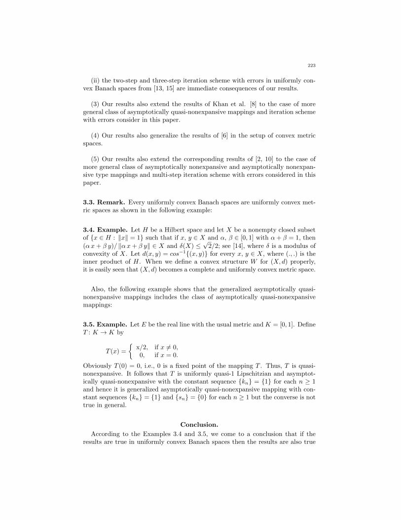
(ii) the two-step and three-step iteration scheme with errors in uniformly con-vex Banach spaces from [13, 15] are immediate consequences of our results.
(3) Our results also extend the results of Khan et al. [8] to the case of moregeneral class of asymptotically quasi-nonexpansive mappings and iteration schemewith errors consider in this paper.
(4) Our results also generalize the results of [6] in the setup of convex metricspaces.
(5) Our results also extend the corresponding results of [2, 10] to the case ofmore general class of asymptotically nonexpansive and asymptotically nonexpan-sive type mappings and multi-step iteration scheme with errors considered in thispaper.
3.3. Remark. Every uniformly convex Banach spaces are uniformly convex met-ric spaces as shown in the following example:
3.4. Example. Let H be a Hilbert space and let X be a nonempty closed subsetof x ∈ H : ‖x‖ = 1 such that if x, y ∈ X and α, β ∈ [0, 1] with α+ β = 1, then
(αx+ β y)/ ‖αx+ β y‖ ∈ X and δ(X) ≤√
2/2; see [14], where δ is a modulus ofconvexity of X. Let d(x, y) = cos−1(x, y) for every x, y ∈ X, where (., .) is theinner product of H. When we define a convex structure W for (X, d) properly,it is easily seen that (X, d) becomes a complete and uniformly convex metric space.
Also, the following example shows that the generalized asymptotically quasi-nonexpansive mappings includes the class of asymptotically quasi-nonexpansivemappings:
3.5. Example. Let E be the real line with the usual metric and K = [0, 1]. DefineT : K → K by
T (x) =
x/2, if x 6= 0,0, if x = 0.
Obviously T (0) = 0, i.e., 0 is a fixed point of the mapping T . Thus, T is quasi-nonexpansive. It follows that T is uniformly quasi-1 Lipschitzian and asymptot-ically quasi-nonexpansive with the constant sequence kn = 1 for each n ≥ 1and hence it is generalized asymptotically quasi-nonexpansive mapping with con-stant sequences kn = 1 and sn = 0 for each n ≥ 1 but the converse is nottrue in general.
Conclusion.
According to the Examples 3.4 and 3.5, we come to a conclusion that if theresults are true in uniformly convex Banach spaces then the results are also true
223

in complete convex metric spaces. Thus our results are good improvement andgeneralization of corresponding results of [2, 4, 6, 7, 9, 11, 12, 15, 16, 17, 20].
Acknowledgement. The author thank the referees for their valuable sugges-tions and comments on the manuscript.
References
[1] S.S. Chang, Y.J. Cho and H.Y. Zhou, Iterative methods for nonlinear operatorequations in Banach spaces, Nova Science Publishers, New York (2002).
[2] S.S. Chang, J.K. Kim and D.S. Jin, Iterative sequences with errors for asymp-totically quasi-nonexpansive type mappings in convex metric spaces, Archivesof Inequality and Applications 2(2004), 365-374.
[3] C.E. Chidume, Convergence theorems for asymptotically pseudocontractivemappings, Nonlinear Anal. 49(2002), no.1, 1-11.
[4] H. Fukhur-ud-din and S.H. Khan, Convergence of iterates with errors ofasymptotically quasi-nonexpansive mappings and applications, J. Math. Anal.Appl. 328(2007), 821-829.
[5] K. Goebel and W.A. Kirk, A fixed point theorem for asymptotically nonexpan-sive mappings, Proc. Amer. Math. Soc. 35(1972), 171-174.
[6] S. Imnang and S. Suantai, Common fixed points of multi-step Noor iterationswith errors for a finite family of generalized asymptotically quasi-nonexpansivemappings, Abstr. Appl. Anal. (2009), Article ID 728510, 14pp.
[7] A.R. Khan, A.A. Domlo and H. Fukhar-ud-din, Common fixed points of Nooriteration for a finite family of asymptotically quasi-nonexpansive mappings inBanach spaces, J. Math. Anal. Appl. 341(2008), 1-11.
[8] A.R. Khan, M.A. Khamsi and H. Fukhar-ud-din, Strong convergence of ageneral iteration scheme in CAT(0) spaces, Nonlinear Anal.: TMA, 74(2011),no.3, 783-791.
[9] S.H. Khan and W. Takahashi, Approximating common fixed points of twoasymptotically nonexpansive mappings, Sci. Math. Jpn. 53(2001), no. 1, 143-148.
[10] J.K. Kim, K.H. Kim and K.S. Kim, Three-step iterative sequences with er-rors for asymptotically quasi-nonexpansive mappings in convex metric spaces,Nonlinear Anal. Convex Anal. RIMS Vol. 1365(2004), pp. 156-165.
[11] Q.H. Liu, Iterative sequences for asymptotically quasi-nonexpansive mappings,J. Math. Anal. Appl. 259(2001), 1-7.
[12] Q.H. Liu, Iterative sequences for asymptotically quasi-nonexpansive mappingswith error member, J. Math. Anal. Appl. 259(2001), 18-24.
[13] Q.H. Liu, Iterative sequences for asymptotically quasi-nonexpansive mappingswith error member of uniformly convex Banach spaces, J. Math. Anal. Appl.266(2002), 468-471.
[14] H.V. Machado, Fixed point theorems for nonexpansive mappings in metricspaces with normal structure, Thesis, The University of Chicago, 1971.
[15] G.S. Saluja, Approximating fixed points of Noor iteration with errors forasymptotically quasi-nonexpansive mappings, Funct. Anal. Appr. Comput.1(2009), no.1, 31-48.
224

[16] J. Schu, Iterative construction of fixed points of asymptotically nonexpansivemappings, J. Math. Anal. Appl. 158(1991), 407-413.
[17] J. Schu, Weak and strong convergence to fixed points of asymptotically non-expansive mappings, Bull. Austral. Math. Soc. 43(1991), no.1, 153-159.
[18] W. Takahashi, A convexity in metric space and nonexpansive mappings I,Kodai Math. Sem. Rep. 22(1970), 142-149.
[19] K.K. Tan and H.K. Xu, Approximating fixed points of nonexpansive mappingsby the Ishikawa iteration process, J. Math. Anal. Appl. 178(1993), 301-308.
[20] B.L. Xu and M.A. Noor, Fixed point iterations for asymptotically nonexpan-sive mappings in Banach spaces, J. Math. Anal. Appl. 267(2002), no.2, 444-453.
[21] Y. Xu, Ishikawa and Mann iterative processes with errors for nonlinearstrongly accretive operator equation, J. Math. Anal. Appl. 224(1998), no.1,91-101.
[22] H. Zhou, J.I. Kang, S.M. Kang and Y.J. Cho, Convergence theorems for uni-formly quasi-Lipschitzian mappings, Int. J. Math. Math. Sci. 15(2004), 763-775.
225


Hacettepe Journal of Mathematics and StatisticsVolume 43 (2) (2014), 227 – 230
A shorter proof of the Smith normal form ofskew-Hadamard matrices
and their designs
Ilhan Hacıoglu∗ and Aytul Keman†
Abstract
We provide a shorter algebraic proof for the Smith normal form ofskew-hadamard matrices and the related designs.
Keywords: p-rank, Hadamard design, Smith normal form.
2000 AMS Classification: 20C08, 51E12, 05B20
1. Introduction
Smith normal forms and p-ranks of designs can help distinguish non-isomorphicdesigns with the same parameters. So it is interesting to know their Smith normalform explicitly. Smith normal forms of some designs were computed in [2],[3] and[5]. In this article we give a shorter proof for the Smith normal form of skew-hadamard matrices and their designs.
A Hadamard matrix H of order n is an n by n matrix whose elements are ±1and which satisfies HHT = nIn. It is skew-Hadamard matrix if, it also satisfiesH + HT = 2In. For more information about the Hadamard matrices please see[1], [9]. Similar definitions stated below can be found in [4], [5], [6], [7], [8], [9].
The incidence matrix of a Hadamard (4m− 1, 2m,m) design D is a 4m− 1 by4m− 1 (0, 1)-matrix A that satisfies
AAT = ATA = mI +mJ.
The complementary design D is a (4m − 1, 2m − 1,m − 1) design with incidencematrix J − A. A skew-hadamard (4m − 1, 2m,m) design is a hadamard designthat satisfies(after some row and column permutations)
A+AT = I + J
∗Department of Mathematics, Arts and Science Faculty Canakkale Onsekiz Mart University,
17100 Canakkale,Turkey, Email: [email protected]†Department of Mathematics, Arts and Science Faculty Canakkale Onsekiz Mart University,
17100 Canakkale,Turkey, Email: [email protected]

Integral Equivalence: If A and B are matrices over the ring Z of integers,A and B are called equivalent (A ∼ B) if there are Z−matrices P and Q, ofdeterminant ±1, such that
B = PAQ
which means that one can be obtained from the other by a sequence of the followingoperations:
• Reorder the rows,• Negate some row,• Add an integer multiple of one row to another,
and the corresponding column operations.
Smith Normal Form: If A is any n by n, Z− matrix, then there is a uniqueZ−matrix
S = diag(a1, a2, ..., an)
such that A ∼ S and
a1|a2|...|ar, ar+1 = . . . = an = 0,
where the ai are non-negative. The greatest common divisor of i by i subdetermi-nants of A is
a1a2a3 . . . ai.
The ai are called invariants factors of A and S is the Smith normal form(SNF (A))of A.p-Rank: The p-rank of an n by n, Z− matrix A is the rank of A over a field
of characteristic p and is denoted by rankp(A). The p-rank of A is related to theinvariant factors a1, a2, ..., an by
rankp(A) = maxi : p does not divide ai
2. Proof of the main theorem
2.1. Proposition. ([6] or [8]): Let H be a Hadamard matrix of order 4m withinvariant factors h1, ..., h4m. Then h1 = 1, h2 = 2, and hih4m+1−i = 4m (i =1, . . . , 4m).
2.2. Theorem. ([7]): Let A, B, C = A+B, be n by n matrices over Z , with in-variant factors h1(A)| . . . |hn(A), h1(B)| . . . |hn(B), h1(C)| . . . |hn(C), respectively.Then
gcd(hi(A), hj(B))|hi+j−1(A+B)
for any indices i, j with 1 ≤ i, j ≤ n , i + j − 1 ≤ n , where gcd denotes greatestcommon divisor.
2.3. Theorem. ([4]): Let D be a skew-Hadamard (4m−1, 2m,m) design. Supposethat p divides m. Then rankp(D) = 2m− 1 and rankp(D) = 2m.
The author in [5] proves the following theorem by using completely differentmethod. Here we provide a shorter algebraic proof for this theorem and the corol-lary following it.
228

2.4. Theorem. A skew-Hadamard matrix of order 4m has Smith normal form
diag[1, 2, . . . , 2︸ ︷︷ ︸2m−1
, 2m, . . . , 2m︸ ︷︷ ︸2m−1
, 4m].
Proof. Applying Theorem 2.2 withA = H andB = HT we get gcd(hi(H), hj(HT ))|2
which means that gcd(hi(H), hj(HT )) = 1 or 2 where 1 ≤ i, j ≤ 4m , i+j−1 ≤ 4m.
If m = 1 then we have a skew-Hadamard matrix of order 4 and by proposition 1 theresult follows. Assume that m > 1 then by proposition 1 we know that h1(H) = 1,h2(H) = 2, h4m−1(H) = 2m and h4m(H) = 4m. Since SNF (H) = SNF (HT )assume that h2m(H) = 2k and h2m(HT ) = 2k where k 6= 1 and k is a divisor ofm. In this case i = j = 2m and Theorem 2.2 gives us gcd(hi(H), hj(H
T )) = 2k|2.But this is a contradiction since k 6= 1. So k = 1 which means that h2m(H) =h2m(HT ) = 2. So all the first 2m elements except the first one have to be 2.Since we found the first 2m elements, using proposition 1 again we obtain theremaining elements namely h2m+1(H) = h2m+2(H) = . . . = h4m−1(H) = 2m andh4m(H) = 4m.
2.5. Corollary. The Smith normal form of the incidence matrix of a skew-Hadamard(4m− 1, 2m,m) design is
diag[1, . . . , 1︸ ︷︷ ︸2m−1
,m, . . . ,m︸ ︷︷ ︸2m−1
, 2m].
Proof. By [5] any skew-Hadamard matrix of order 4m is integrally equivalent to[1] ⊕ (2A). This means that all the invariant factors of A are half of the corre-sponding invariant factors of H except the first one. So the result follows.
Note that we know from Theorem 2.3 that rankpA = 2m−1 which agrees withour result.
By using similar techniques that we used above we get the Smith normal formof the complementary skew-Hadamard design:
2.6. Corollary. The Smith normal form of the incidence matrix of a skew-Hadamard(4m− 1, 2m− 1,m− 1) design is
diag[1, . . . , 1︸ ︷︷ ︸2m
,m, . . . ,m︸ ︷︷ ︸2m−2
,m(2m− 1)].
References
[1] Horadam, K.J. Hadamard Matrices and their Applications, Princeton University Press,
Princeton, (2010).
[2] Koukouvinos, C., Mitrouli, M., Seberry, J. On the Smith Normal form of D-optimal designs,Linear Algebra Appl., 247, 277-295, (1996).
[3] Koukouvinos, C., Mitrouli, M., Seberry, J. On the Smith Normal form of weighing matrices,Bull. Inst. Combin. Appl., 19, 57-69, (1997).
[4] Michael, T.S. The p-Ranks of Skew Hadamard Designs, J. Combin. Theory, Ser.A 73, 170-
171, (1996).[5] Michael, T.S., Wallis, W.D. Skew-Hadamard Matrices and the Smith Normal Form, Designs,
Codes and Cryptography 13, 173-176, (1998).
[6] Newman, M. Invariant Factors of Combinatorial Matrices, Israel J. Math. 10, 126-130,(1971).
229

[7] Thompson, R.C. The Smith Invariants of a Matrix Sum, Proc. Amer. Math. Soc. 78, 162-164,
(1980).
[8] Wallis, W.D., Wallis, J. Equivalence of Hadamard Matrices, Israel J. Math. 7, 122-128, (1969).[9] Wallis, W.D. Combinatorial Designs, Marcel Dekker, New York, (1988).
230

Hacettepe Journal of Mathematics and StatisticsVolume 43 (2) (2014), 231 – 247
Base and subbase in intuitionistic I-fuzzytopological spaces
Chengyu Liang∗ and Conghua Yan †
Abstract
In this paper, the concepts of the base and subbase in intuitionistic I-fuzzy topological spaces are introduced, and use them to discuss fuzzycontinuous mapping and fuzzy open mapping. We also study the baseand subbase in the product of intuitionistic I-fuzzy topological spaces,and T2 separation in product intuitionistic I-fuzzy topological spaces.Finally, the relation between the generated product intuitionistic I-fuzzy topological spaces and the product generated intuitionistic I-fuzzy topological spaces are studied.
Keywords: Intuitionistic I-fuzzy topological space; Base; Subbase; T2 separa-tion; Generated Intuitionistic I-fuzzy topological spaces.
2000 AMS Classification: 54A40
1. Introduction
As a generalization of fuzzy sets, the concept of intuitionistic fuzzy sets wasfirst introduced by Atanassov [1]. From then on, this theory has been studiedand applied in a variety areas ([4, 14, 18], etc). Among of them, the research ofthe theory of intuitionistic fuzzy topology is similar to the the theory of fuzzytopology. In fact, Coker [4] introduced the concept of intuitionistic fuzzy topo-logical spaces, this concept is originated from the fuzzy topology in the sense ofChang [3](in this paper we call it intuitionistic I-topological spaces). Based onCoker’s work [4], many topological properties of intuitionistic I-topological spaceshas been discussed ([5, 10, 11, 12, 13]). On the other hand, Sostak [17] proposeda new notion of fuzzy topological spaces, and this new fuzzy topological structurehas been accepted widely. Influenced by Sostak’s work [17], Coker [7] gave thenotion of intuitionistic fuzzy topological spaces in the sense of Sostak. By thestandardized terminology introduced in [16], we will call it intuitionistic I-fuzzy
∗Department of Mathematics, School of Science, Beijing Institute of Technology, Beijing
100081, PR China, Email: [email protected]†Corresponding Author, Institute of Math., School oh Math. Sciences, Nanjing Normal Uni-
versity, Nanjing, Jiangsu 210023, PR China,
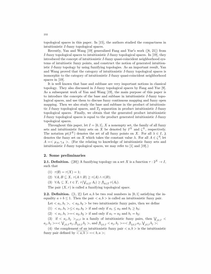
topological spaces in this paper. In [15], the authors studied the compactness inintuitionistic I-fuzzy topological spaces.
Recently, Yan and Wang [19] generalized Fang and Yue′s work ([8, 21]) fromI-fuzzy topological spaces to intuitionistic I-fuzzy topological spaces. In [19], theyintroduced the concept of intuitionistic I-fuzzy quasi-coincident neighborhood sys-tems of intuitiostic fuzzy points, and construct the notion of generated intuition-istic I-fuzzy topology by using fuzzifying topologies. As an important result, Yanand Wang proved that the category of intuitionistic I-fuzzy topological spaces isisomorphic to the category of intuitionistic I-fuzzy quasi-coincident neighborhoodspaces in [19].
It is well known that base and subbase are very important notions in classicaltopology. They also discussed in I-fuzzy topological spaces by Fang and Yue [9].As a subsequent work of Yan and Wang [19], the main purpose of this paper isto introduce the concepts of the base and subbase in intuitionistic I-fuzzy topo-logical spaces, and use them to discuss fuzzy continuous mapping and fuzzy openmapping. Then we also study the base and subbase in the product of intuitionis-tic I-fuzzy topological spaces, and T2 separation in product intuitionistic I-fuzzytopological spaces. Finally, we obtain that the generated product intuitionisticI-fuzzy topological spaces is equal to the product generated intuitionistic I-fuzzytopological spaces.
Throughout this paper, let I = [0, 1], X a nonempty set, the family of all fuzzysets and intuitionistic fuzzy sets on X be denoted by IX and ζX , respectively.The notation pt(IX) denotes the set of all fuzzy points on X. For all λ ∈ I, λdenotes the fuzzy set on X which takes the constant value λ. For all A ∈ ζX, letA =< µA, γA >. (For the relating to knowledge of intuitionistic fuzzy sets andintuitionistic I-fuzzy topological spaces, we may refer to [1] and [19].)
2. Some preliminaries
2.1. Definition. ([20]) A fuzzifying topology on a set X is a function τ : 2X → I,such that
(1) τ(∅) = τ(X) = 1;
(2) ∀A,B ⊆ X, τ(A ∧B) ≥ τ(A) ∧ τ(B);
(3) ∀At ⊆ X, t ∈ T , τ(∨t∈T At) ≥
∧t∈T τ(At).
The pair (X, τ) is called a fuzzifying topological space.
2.2. Definition. ([1, 2]) Let a, b be two real numbers in [0, 1] satisfying the in-equality a+ b ≤ 1. Then the pair < a, b > is called an intuitionistic fuzzy pair.
Let < a1, b1 >, < a2, b2 > be two intuitionistic fuzzy pairs, then we define
(1) < a1, b1 >≤< a2, b2 > if and only if a1 ≤ a2 and b1 ≥ b2;
(2) < a1, b1 >=< a2, b2 > if and only if a1 = a2 and b1 = b2;
(3) if < aj , bj >j∈J is a family of intuitionistic fuzzy pairs, then∨j∈J <
aj , bj >=<∨j∈J aj ,
∧j∈J bj >, and
∧j∈J < aj , bj >=<
∧j∈J aj ,
∨j∈J bj >;
(4) the complement of an intuitionistic fuzzy pair < a, b > is the intuitionisticfuzzy pair defined by < a, b > =< b, a >;
232

In the following, for convenience, we will use the symbols 1∼ and 0∼ denote theintuitionistic fuzzy pairs < 1, 0 > and < 0, 1 >. The family of all intuitionisticfuzzy pairs is denoted by A. It is easy to find that the set of all intuitionistic fuzzypairs with above order forms a complete lattice, and 1∼, 0∼ are its top elementand bottom element, respectively.
2.3. Definition. ([4]) Let X,Y be two nonempty sets and f : X → Y a function,if B = < y, µB(y), γB(y) >: y ∈ Y ∈ ζY, then the preimage of B under f ,denoted by f←(B), is the intuitionistic fuzzy set defined by
f←(B) = < x, f←(µB)(x), f←(γB)(x) >: x ∈ X.Here f←(µB)(x) = µB(f(x)), f←(γB)(x) = γB(f(x)). (This notation is from[16]).
If A = < x, µA(x), γA(x) >: x ∈ X ∈ ζX, then the image A under f , denotedby f→(A) is the intuitionistic fuzzy set defined by
f→(A) = < y, f→(µA)(y), (1− f→(1− γA))(y) >: y ∈ Y .Where
f→(µA)(y) =
supx∈f←(y) µA(x), if f←(y) 6= ∅,
0, if f←(y) = ∅.
1− f→(1− γA)(y) =
infx∈f←(y) γA(x), if f←(y) 6= ∅,
1, if f←(y) = ∅.
2.4. Definition. ([7]) Let X be a nonempty set, δ : ζX → A satisfy the following:
(1) δ(< 0, 1 >) = δ(< 1, 0 >) = 1∼;
(2) ∀A, B ∈ ζX , δ(A∧B) ≥ δ(A)∧δ(B);
(3) ∀At ∈ ζX , t ∈ T , δ(∨t∈T At) ≥
∧t∈T δ(At).
Then δ is called an intuitionistic I-fuzzy topology on X, and the pair (X, δ)is called an intuitionistic I-fuzzy topological space. For any A ∈ ζX, we alwayssuppose that δ(A) =< µδ(A), γδ(A) > later, the number µδ(A) is called theopenness degree of A, while γδ(A) is called the nonopenness degree of A. Afuzzy continuous mapping between two intuitionistic I-fuzzy topological spaces(ζX, δ1) and (ζY, δ2) is a mapping f : X → Y such that δ1(f←(A)) ≥ δ2(A). Thecategory of intuitionistic I-fuzzy topological spaces and fuzzy continuous mappingsis denoted by II-FTOP.
2.5. Definition. ([6, 11, 12]) Let X be a nonempty set. An intuitionistic fuzzypoint, denoted by x(α,β), is an intuitionistic fuzzy set A = < y, µA(y), γA(y) >:y ∈ X, such that
µA(y) =
α, if y = x,0, if y 6= x.
and
γA(y) =
β, if y = x,1, if y 6= x.
233

Where x ∈ X is a fixed point, the constants α ∈ I0, β ∈ I1 and α + β ≤ 1. Theset of all intuitionistic fuzzy points x(α,β) is denoted by pt(ζX).
2.6. Definition. ([12]) Let x(α,β) ∈ pt(ζX) and A, B ∈ ζX. We say x(α,β)
quasi-coincides with A, or x(α,β) is quasi-coincident with A, denoted x(α,β)qA, ifµA(x) + α > 1 and γA(x) + β < 1. Say A quasi-coincides with B at x, or say Ais quasi-coincident with B at x, AqB at x, in short, if µA(x) + µB(x) > 1 andγA(x) + γB(x) < 1. Say A quasi-coincides with B, or A is quasi-coincident withB, if A is quasi-coincident with B at some point x ∈ X.Relation“does not quasi-coincides with” or “is not quasi-coincident with ” is de-noted by ¬q.
It is easily to know for ∀x(α,β) ∈ pt(ζX), x(α,β)q < 1, 0 > and x(α,β)¬q < 0, 1 >.
2.7. Definition. ([19]) Let (X, δ) be an intuitionistic I-fuzzy topological space.For all x(α,β) ∈ pt(ζX), U ∈ ζX , the mapping Qδx(α,β)
: ζX → A is defined as
follows
Qδx(α,β)(U) =
∨x(α,β)q V≤U
δ(V ), x(α,β)q U ;
0∼, x(α,β)¬q U.The set of Qδ = Qδx(α,β)
: x(α,β) ∈ pt(ζX) is called intuitionistic I-fuzzy quasi-
coincident neighborhood system of δ on X.
2.8. Theorem. ([19]) Let (X, δ) be an intuitionistic I-fuzzy topological space,Qδ = Qδx(α,β)
: x(α,β) ∈ pt(ζX) of maps Qδx(α,β): ζX → A defined in Definition
2.7 satisfies: ∀U, V ∈ ζX ,
(1) Qδx(α,β)(〈1, 0〉) = 1∼, Qδx(α,β)
(〈0, 1〉) = 0∼;
(2) Qδx(α,β)(U) > 0∼ ⇒ x(α,β)q U ;
(3) Qδx(α,β)(U ∧ V ) = Qδx(α,β)
(U) ∧Qδx(α,β)(V );
(4) Qδx(α,β)(U) =
∨x(α,β)q V≤U
∧y(λ,ρ)q V
Qδy(λ,ρ)(V );
(5) δ(U) =∧
x(α,β)q U
Qδx(α,β)(U).
2.9. Lemma. ([21]) Suppose that (X, τ) is a fuzzifying topological space, for eachA ∈ IX, let ω(τ)(A) =
∧r∈I τ(σr(A)), where σr(A) = x : A(x) > r. Then ω(τ)
is an I-fuzzy topology on X, and ω(τ) is called induced I-fuzzy topology determinedby fuzzifying topology τ .
2.10. Definition. ([19]) Let (X, τ) be a fuzzifying topological space, ω(τ) is aninduced I-fuzzy topology determined by fuzzifying topology τ . For each A ∈ ζX, letIω(τ)(A) =< µτ (A), γτ (A) >, where µτ (A) = ω(τ)(µA) ∧ ω(τ)(1− γA), γτ (A) =1−µτ (A).We say that (ζX, Iω(τ)) is a generated intuitionistic I-fuzzy topologicalspace by fuzzifying topological space (X, τ).
2.11. Lemma. ([19]) Let (X, τ) be a fuzzifying topological space, then
(1) ∀A ⊆ X, µτ (< 1A, 1Ac >) = τ(A).
(2) ∀A =< α, β >∈ ζX , Iω(τ)(A) = 1∼.
234

2.12. Lemma. ([19]) Suppose that (ζX, δ) is an intuitionistic I-fuzzy topologicalspace, for each A ⊆ X, let [δ](A) = µδ(< 1A, 1Ac >). Then [δ] is a fuzzifyingtopology on X.
2.13. Lemma. ([19]) Let (X, τ) be a fuzzifying topological space and (X, Iω(τ)) agenerated intuitionistic I-fuzzy topological space. Then [Iω(τ)] = τ .
3. Base and subbase in Intuitionistic I-fuzzy topological spaces
3.1. Definition. Let (X, τ) be an intuitionistic I-fuzzy topological space andB : ζX → A. B is called a base of τ if B satisfies the following condition
τ(U) =∨
∨λ∈K
Bλ=U
∧
λ∈KB(Bλ),∀ U ∈ ζX .
3.2. Definition. Let (X, τ) be an intuitionistic I-fuzzy topological space andϕ : ζX → A, ϕ is called a subbase of τ if ϕ(u) : ζX → A is a base, whereϕ(u)(A) =
∨uBλ:λ∈E=A
∧λ∈E
ϕ(Bλ), for all A ∈ ζX with (u) standing for “finite
intersection”.
3.3. Theorem. Suppose that B : ζX → A. Then B is a base of some intuitionisticI-fuzzy topology, if B satisfies the following condition
(1) B(0∼) = B(1∼) = 1∼,
(2) ∀ U, V ∈ ζX , B(U ∧ V ) ≥ B(U) ∧B(V ).
Proof. For ∀ A ∈ ζX , let τ(A) =∨
∨λ∈K
Bλ=A
∧λ∈K
B(Bλ). To show that B is a base
of τ , we only need to prove τ is an intuitionistic I-fuzzy topology on X. For allU, V ∈ ζX ,
τ(U) ∧ τ(V ) =( ∨
∨α∈K1
Aα=U
∧
α∈K1
B(Aα))∧( ∨
∨β∈K2
Bβ=V
∧
β∈K2
B(Bβ))
=∨
∨α∈K1
Aα=U,∨
β∈K2
Bβ=V
(( ∧
α∈K1
B(Aα))∧( ∧
β∈K2
B(Bβ)))
≤∨
∨α∈K1,β∈K2
(Aα∧Bβ)=U∧V
( ∧
α∈K1,β∈K2
B(Aα ∧Bβ))
≤∨
∨λ∈K
Cλ=U∧V
∧
λ∈KB(Cλ)
= τ(U ∧ V ).
For all Aλ : λ ∈ K ⊆ ζX , Let Bλ = Bδλ : δλ ∈ Kλ :∨
δλ∈KλBδλ = Aλ, then
τ(∨
λ∈KAλ) =
∨∨
δ∈K1
Bδ=∨λ∈K
Aλ
∧
δ∈K1
B(Bδ).
235

For all f ∈ ∏λ∈K
Bλ, we have
∨
λ∈K
∨
Bδλ∈f(λ)
Bδλ =∨
λ∈KAλ.
Therefore,
µτ(∨λ∈K
Aλ) =∨
∨δ∈K1
Bδ=∨λ∈K
Aλ
∧
δ∈K1
µB(Bδ)
≥∨
f∈ ∏λ∈K
Bλ
∧
λ∈K
∧
Bδλ∈f(λ)
µB(Bδλ )
=∧
λ∈K
∨
Bδλ :δλ∈Kλ∈Bλ
∧
δλ∈KλµB(Bδλ )
=∧
λ∈Eµτ(Aλ).
Similarly, we have
γτ(∨λ∈K
Aλ) ≤∨
λ∈Kγτ(Aλ).
Hence
τ(∨
λ∈KAλ) ≥
∧
λ∈Kτ(Aλ).
This means that τ is an intuitionistic I-fuzzy topology on X and B is a base ofτ .
3.4. Theorem. Let (X, τ), (Y, δ) be two intuitionistic I-fuzzy topology spacesand δ generated by its subbase ϕ. The mapping f : (X, τ) → (Y, δ) satisfiesϕ(U) ≤ τ(f←(U)), for all U ∈ ζY . Then f is fuzzy continuous, i.e., δ(U) ≤τ(f←(U)),∀ U ∈ ζY .
Proof. ∀ U ∈ ζY ,
δ(U) =∨
∨λ∈K
Aλ=U
∧
λ∈K
∨
uBµ:µ∈Kλ=Aλ
∧
µ∈Kλϕ(Bµ)
≤∨
∨λ∈K
Aλ=U
∧
λ∈K
∨
uBµ:µ∈Kλ=Aλ
∧
µ∈Kλτ(f←(Bµ))
≤∨
∨λ∈K
Aλ=U
∧
λ∈Kτ(f←(Aλ))
≤∨
∨λ∈K
Aλ=U
τ(f←(∨
λ∈KAλ))
= τ(f←(U)).
This completes the proof.
236

3.5. Theorem. Suppose that (X, τ), (Y, δ) are two intuitionistic I-fuzzy topologyspaces and τ is generated by its base B. If the mapping f : (X, τ)→ (Y, δ) satisfiesB(U) ≤ δ(f→(U)), for all U ∈ ζX . Then f is fuzzy open, i.e., ∀ W ∈ ζX , τ(W ) ≤δ(f→(W )).
Proof. ∀ W ∈ ζX ,
τ(W ) =∨
∨λ∈K
Aλ=W
∧
λ∈KB(Aλ)
≤∨
∨λ∈K
Aλ=W
∧
λ∈Kδ(f→(Aλ))
≤∨
∨λ∈K
Aλ=W
δ(f→(∨
λ∈KAλ))
= δ(f→(W )).
Therefore, f is open.
3.5. Theorem. Let (X, τ), (Y, δ) be two intuitionistic I-fuzzy topology spacesand f : (X, τ) → (Y, δ) intuitionistic I-fuzzy continuous, Z ⊆ X. Then f |Z :(Z, τ |Z) → (Y, δ) is continuous, where (f |Z)(x) = f(x), (τ |Z)(A) = ∨τ(U) :U |Z = A, for all x ∈ Z,A ∈ ζZ .
Proof. ∀ W ∈ ζZ , (f |Z)←(W ) = f←(W )|Z , we have
(τ |Z)((f |Z)←(W )) = ∨τ(U) : U |Z = (f |Z)←(W )≥ τ(f←(W ))
≥ δ(W ).
Then f |Z is intuitionistic I-fuzzy continuous.
3.6. Theorem. Let (X, τ) be an intuitionistic I-fuzzy topology space and τ gen-erated by its base B, B|Y (U) = ∨B(W ) : W |Y = U, for Y ⊆ X,U ∈ ζY . ThenB|Y is a base of τ |Y .
Proof. For ∀ U ∈ ζX , (τ |Y )(U) =∨
V |Y =U
τ(V ) =∨
V |Y =U
∨∨λ∈K
Aλ=V
∧λ∈K
B(Aλ). It
remains to show the following equality∨
V |Y =U
∨∨λ∈K
Aλ=V
∧
λ∈KB(Aλ) =
∨∨λ∈K
Bλ=U
∧
λ∈K
∨
W |Y =Bλ
B(W ).
In one hand, for all V ∈ ζX with V |Y = U, and∨λ∈K
Aλ = V, we have∨λ∈K
Aλ|Y = U. Put Bλ = Aλ|Y , clearly∨λ∈K
Bλ = U. Then
∨∨λ∈K
Bλ=U
∧
λ∈K
∨
W |Y =Bλ
B(W ) ≥∧
λ∈KB(Aλ).
237

Thus, ∨
V |Y =U
∨∨λ∈K
Aλ=V
∧
λ∈KB(Aλ) ≤
∨∨λ∈K
Bλ=U
∧
λ∈K
∨
W |Y =Bλ
B(W ).
On the other hand, ∀ a ∈ (0, 1], a <∨
∨λ∈K
Bλ=U
∧λ∈K
∨W |Y =Bλ
µB(W ), there exists a
family of Bλ : λ ∈ K ⊆ ζY , such that
(1)∨λ∈K
Bλ = U ;
(2) ∀ λ ∈ K, there exists Wλ ∈ ζX with Wλ|Y = Bλ such that a <µB(Wλ).
Let V =∨λ∈E
Wλ, it is clear V |Y = U and∧λ∈K
µB(Wλ) ≥ a. Then
∨
V |Y =U
∨∨λ∈K
Aλ=V
∧
λ∈KµB(Aλ) ≥ a.
By the arbitrariness of a, we have∨
V |Y =U
∨∨λ∈K
Aλ=V
∧
λ∈KµB(Aλ) ≥
∨∨λ∈K
Bλ=U
∧
λ∈K
∨
W |Y =Bλ
µB(W ).
Similarly, we may obtain that∧
V |Y =U
∧∨λ∈K
Aλ=V
∨
λ∈KγB(Aλ) ≤
∧∨λ∈K
Bλ=U
∨
λ∈K
∧
W |Y =Bλ
γB(W ).
So we have∨
V |Y =U
∨∨λ∈K
Aλ=V
∧
λ∈KB(Aλ) ≥
∨∨λ∈K
Bλ=U
∧
λ∈K
∨
W |Y =Bλ
B(W ).
Therefore,∨
V |Y =U
∨∨λ∈K
Aλ=V
∧
λ∈KB(Aλ) =
∨∨λ∈K
Bλ=U
∧
λ∈K
∨
W |Y =Bλ
B(W ).
This means that B|Y is a base of τ |Y .
3.7. Theorem. Let (Xα, τα)α∈J be a family of intuitionistic I-fuzzy topology
spaces and Pβ :∏α∈J
Xα → Xβ the projection. For all W ∈ ζ
∏α∈J
Xα, ϕ(W ) =
∨α∈J
∨P←α (U)=W
τα(U). Then ϕ is a subbase of some intuitionistic I-fuzzy topology τ ,
here τ is called the product intuitionistic I-fuzzy topologies of τα : α ∈ J anddenoted by τ =
∏α∈J
τα.
238

Proof. We need to prove ϕ(u) is a subbase of τ .
ϕ(u)(1∼) =∨
uBλ:λ∈E=1∼
∧
λ∈Eϕ(Bλ)
=∨
uBλ:λ∈E=1∼
∧
λ∈E
∨
α∈J
∨
P←α (U)=Bλ
τα(U)
= 1∼.
Similarly, ϕ(u)(0∼) = 1∼. For all U, V ∈ ζ∏α∈J
Xα, we have
ϕ(u)(U) ∧ ϕ(u)(V ) =( ∨
uBα:α∈E1=U
∧
α∈E1
ϕ(Bα))∧( ∨
uCβ :β∈E2=V
∧
β∈E2
ϕ(Cβ))
=∨
uBα:α∈E1=U
∨
uCβ :β∈E2=V
((∧
α∈E1
ϕ(Bα)) ∧ (∧
β∈E2
ϕ(Cβ)))
≤∨
uBλ:λ∈E=U∧V
∧
λ∈Eϕ(Bλ)
= ϕ(u)(U ∧ V ).
Hence, ϕ(u)is a base of τ , i.e., ϕ is a subbase of τ . And by Theorem 3.3 we have
τ(A) =∨
∨λ∈K
Bλ=A
∧
λ∈Kϕ(u)(Bλ)
=∨
∨λ∈K
Bλ=A
∧
λ∈K
∨
uCρ:ρ∈E=Bλ
∧
ρ∈Eϕ(Cρ)
=∨
∨λ∈K
Bλ=A
∧
λ∈K
∨
uCρ:ρ∈E=Bλ
∧
ρ∈E
∨
α∈J
∨
P←α (V )=Cρ
τα(V ).
By the above discussions, we easily obtain the following corollary.
3.8. Corollary. Let (∏α∈J
Xα,∏α∈J
τα) be the product space of a family of intu-
itionistic I-fuzzy topology spaces (Xα, τα)α∈J . Then Pβ : (∏α∈J
Xα,∏α∈J
τα) →(Xβ , τβ) is continuous, for all β ∈ J .
Proof. ∀ U ∈ ζXβ ,
τ(P←β (U)) =∨
∨λ∈K
Bλ=P←β (U)
∧
λ∈K
∨
uCρ:ρ∈E=Bλ
∧
ρ∈E
∨
α∈J
∨
P←α (V )=Cρ
τα(V )
≥ τβ(U)
Therefore, Pβ is continuous.
239
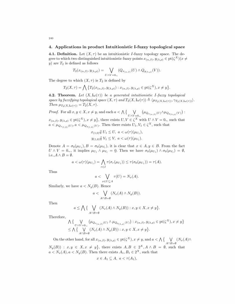
4. Applications in product Intuitionistic I-fuzzy topological space
4.1. Definition. Let (X, τ) be an intuitionistic I-fuzzy topology space. The de-gree to which two distinguished intuitionistic fuzzy points x(α,β), y(λ,ρ) ∈ pt(ζX)(x 6=y) are T2 is defined as follows
T2(x(α,β), y(λ,ρ)) =∨
U∧V=0∼
(Qx(α,β)(U) ∧Qy(λ,ρ)(V )).
The degree to which (X, τ) is T2 is defined by
T2(X, τ) =∧
T2(x(α,β), y(λ,ρ)) : x(α,β), y(λ,ρ) ∈ pt(ζX), x 6= y.
4.2. Theorem. Let (X, Iω(τ)) be a generated intuitionistic I-fuzzy topological
space by fuzzifying topological space (X, τ) and T2(X, Iω(τ)) , 〈µT2(X,Iω(τ)), γT2(X,Iω(τ))〉.Then µT2(X,Iω(τ)) = T2(X, τ).
Proof. For all x, y ∈ X,x 6= y, and each a <∧ ∨
U∧V=0∼
(µQx(α,β) (U)∧µQy(λ,ρ) (V )
):
x(α,β), y(λ,ρ) ∈ pt(ζX), x 6= y
, there exists U, V ∈ ζX with U ∧ V = 0∼ such that
a < µQx(1,0) (U), a < µQy(1,0) (V ). Then there exists U1, V1 ∈ ζX , such that
x(1,0)q U1 ≤ U, a < ω(τ)(µU1),
y(1,0)q V1 ≤ V, a < ω(τ)(µV1).
Denote A = σ0(µU1), B = σ0(µV1
), it is clear that x ∈ A, y ∈ B. From the factU ∧ V = 0∼, it implies µU1
∧ µV1= 0. Then we have σ0(µU1
) ∧ σ0(µV1) = ∅,
i.e.,A ∧B = ∅.a < ω(τ)(µU1
) =∧
r∈Iτ(σr(µU1
)) ≤ τ(σ0(µU1)) = τ(A).
Thusa <
∨
x∈U⊆Aτ(U) = Nx(A).
Similarly, we have a < Ny(B). Hence
a <∨
A∩B=∅(Nx(A) ∧Ny(B)).
Thena ≤
∧ ∨
A∩B=∅(Nx(A) ∧Ny(B)) : x, y ∈ X,x 6= y
.
Therefore, ∧ ∨U∧V=0∼
(µQx(α,β) (U) ∧ µQy(λ,ρ) (V )
): x(α,β), y(λ,ρ) ∈ pt(ζX), x 6= y
≤ ∧ ∨A∩B=∅
(Nx(A) ∧Ny(B)) : x, y ∈ X,x 6= y.
On the other hand, for all x(α,β), y(λ,ρ) ∈ pt(ζX), x 6= y, and a <∧ ∨
A∩B=∅(Nx(A)∧
Ny(B)) : x, y ∈ X,x 6= y, there exists A,B ∈ 2X , A ∧ B = ∅, such that
a < Nx(A), a < Ny(B). Then there exists A1, B1 ∈ 2X , such that
x ∈ A1 ⊆ A, a < τ(A1),
240

y ∈ B1 ⊆ B, a < τ(B1).
Let U = 〈1A1, 1Ac1〉, V = 〈1B1
, 1Bc1 〉, where Ac1 is the complement of A1, thenx(α,β)q U, y(λ,ρ)q V . In fact, 1A1(x) = 1 > 1 − α, 1Ac1(x) = 0 < 1 − β. Thusx(α,β)q U . Similarly, we have y(λ,ρ)q V . By A∧B = ∅, we have A1∧B1 = ∅. Thenfor all z ∈ X, we obtain
(1A1∧ 1B1
)(z) = 1A1(z) ∧ 1B1
(z) = 0,
(1Ac1 ∨ 1Bc1 )(z) = 1Ac1(z) ∨ 1Bc1 (z) = 1.
Hence
1A1∧ 1B1
= 0, 1Ac1 ∨ 1Bc1 = 1.
Since ∀ r ∈ I1, σr(1A1) = A1, we have
ω(τ)(1A1) =
∧
r∈I1τ(σr(1A1
)) = τ(A1).
By 1− 1Ac1 = 1A1 , and a < τ(A1), we have
a < ω(τ)(1A1) ∧ ω(τ)(1− 1Ac1)
= ω(τ)(µU ) ∧ ω(τ)(1− γU ).
So,
a <∨
x(α,β)q W⊆U(ω(τ)(µW ) ∧ ω(τ)(1− γW )) = µQx(α,β) (U).
Similarly, we have a < µQy(λ,ρ) (V ). This deduces that
a <∨
U∧V=0∼
(µQx(α,β) (U) ∧ µQy(λ,ρ) (V )
).
Furthermore, we may obtain
a ≤∧ ∨
U∧V=0∼
(µQx(α,β) (U) ∧ µQy(λ,ρ) (V )
): x(α,β), y(λ,ρ) ∈ pt(ζX), x 6= y
.
Hence ∧ ∨U∧V=0∼
(µQx(α,β) (U) ∧ µQy(λ,ρ) (V )
): x(α,β), y(λ,ρ) ∈ pt(ζX), x 6= y
≥ ∧ ∨A∩B=∅
(Nx(A) ∧Ny(B)) : x, y ∈ X,x 6= y.
This means that∧ ∨
U∧V=0∼
(µQx(α,β) (U)∧µQy(λ,ρ) (V )
): x(α,β), y(λ,ρ) ∈ pt(ζX), x 6=
y
=∧ ∨
A∩B=∅(Nx(A) ∧Ny(B)) : x, y ∈ X,x 6= y
. Therefore we have
µT2(X,Iω(τ)) = T2(X, τ).
4.3. Lemma. Let (∏j∈J
Xj ,∏j∈J
τj) be the product space of a family of intuitionistic
I-fuzzy topology spaces (Xj , τj)j∈J . Then τj(Aj) ≤ (∏j∈J
τj)(P←j (Aj)), for all
j ∈ J,Aj ∈ ζXj .
241

Proof. Let∏j∈J
τj = δ, x(α,β)q f←(U) ⇔ f→(x(α,β))q U . Then for all j ∈ J,Aj ∈
ζXj , we have
δ(P←j (Aj)) =∧
x(α,β)q P←j (Aj)
Qδx(α,β)(P←j (Aj))
≥∧
x(α,β)q P←j (Aj)
QτjP→j (x(α,β))
(Aj)
=∧
P→j (x(α,β))q Aj
QτjP→j (x(α,β))
(Aj)
≥∧
xj(α,β)
q Aj
Qτj
xj(α,β)
(Aj)
= τj(Aj).
This completes the proof.
4.4. Theorem. Let (∏j∈J
Xj ,∏j∈J
τj) be the product space of a family of intuitionis-
tic I-fuzzy topology spaces (Xj , τj)j∈J . Then∧j∈J
T2(Xj , τj) ≤ T2(∏j∈J
Xj ,∏j∈J
τj).
Proof. For all g(α,β), h(λ,ρ) ∈ pt(ζ
∏j∈J
Xj) and g 6= h. Then there exists j0 ∈ J such
that g(j0) 6= h(j0), where g(j0), h(j0) ∈ Xj0 .
For all Uj0 , Vj0 ∈ ζXj0 with Uj0 ∧ Vj0 = 0Xj0∼ , we have
P←j0 (Uj0) ∧ P←j0 (Vj0) = P←j0 (Uj0 ∧ Vj0) = 0
∏j∈J
Xj
∼ .
ThenQg(j0)(α,β)(Uj0) ≤ Qg(α,β)(P←j0 (Uj0)). In fact, if g(j0)(α,β)q Uj0 , then g(α,β)q P←j0
(Uj0).
For all V ≤ Uj0 , we have P←j0 (V ) ≤ P←j0 (Uj0). On account of Lemma 4.3, we have
∨
g(j0)(α,β)q V≤Uj0
τj0(V ) ≤∨
g(α,β)q P←j0
(V )≤P←j0 (Uj0 )
(∏
j∈Jτj)(P
←j0 (V ))
≤∨
g(α,β)q G≤P←j0 (Uj0 )
(∏
j∈Jτj)(G),
i.e., Qg(j0)(α,β)(Uj0) ≤ Qg(α,β)(P←j0 (Uj0)). Thus,∨
U∧V=0Xj0∼
(Qg(j0)(α,β)(U) ∧Qh(j0)(λ,ρ)(V ))
≤ ∨
P←j0 (U)∧P←j0 (V )=0
∏j∈J
Xj
∼
(Qg(α,β)(P←j0
(U))∧Qh(λ,ρ)(P←j0 (V )))
≤ ∨
G∧H=0
∏j∈J
Xj
∼
(Qg(α,β)(G) ∧Qh(λ,ρ)(H)).
242

So we have
T2(g(j0)(α,β), h(j0)(λ,ρ)) ≤ T2(g(α,β), h(λ,ρ)).
Thus
T2(Xj0 , τj0) ≤ T2(∏
j∈JXj ,
∏
j∈Jτj).
Therefore, ∧
j∈JT2(Xj , τj) ≤ T2(
∏
j∈JXj ,
∏
j∈Jτj).
4.5. Lemma. Let (X, Iω(τ)) be a generated intuitionistic I-fuzzy topological spaceby fuzzifying topological space (X, τ). Then
(1) Iω(τ)(A) = 1∼, for all A = 〈α, β〉 ∈ ζX ;
(2) ∀ B ⊆ X, τ(B) = µIω(τ)(〈1B , 1Bc〉).Proof. By Lemma 2.11, 2.12 and 2.13, it is easy to prove it.
4.6. Lemma. Let (X, δ) be a stratified intuitionistic I-fuzzy topological space (i.e.,for all < α, β >∈ A, δ(< α, β >) = 1∼). Then for all A ∈ ζX
∧r∈I
µδ(〈1σr(µA), 1(σr(µA))c〉) ≤ µδ(A).
Proof. For all A ∈ ζX , and for any a <∧r∈I
µδ(〈1σr(µA), 1(σr(µA))c〉), y(α,β) ∈
pt(ζX) with y(α,β)q A, clearly µA(y) > 1 − α. Then there exists δ > 0 such thatµA(y) > 1− α+ δ. Thus y ∈ σ1−α+δ(µA). So we have
y(α,β)q 〈1σ1−α+δ(µA), 1(σ1−α+δ(µA))c〉.Then
a < µδ(〈1σ1−α+δ(µA), 1(σ1−α+δ(µA))c〉)
=∧
z(α,β)q 〈1σ1−α+δ(µA),1(σ1−α+δ(µA))c 〉µ(Qz(α,β)(〈1σ1−α+δ(µA), 1(σ1−α+δ(µA))c〉)).
Therefore,
a < µ(Qy(α,β)(〈1σ1−α+δ(µA), 1(σ1−α+δ(µA))c〉)).
Since (X, δ) is a stratified intuitionistic I-fuzzy topological space, we haveQy(α,β)(1− α+ δ, α− δ〉) = 1∼. Moreover, it is well known that the followingrelations hold
1− α+ δ ∧ 1σ1−α+δ(µA) ≤ µA,
α− δ ∨ 1(σ1−α+δ(µA))c ≥ 1− µA ≥ γA.
So we have
a < µ(Qy(α,β)(〈1− α+ δ∧1σ1−α+δ(µA), α− δ∨1(σ1−α+δ(µA))c〉)) ≤ µ(Qy(α,β)(A)).
243

Then a ≤ µδ(A). Therefore,∧
r∈Iµδ(〈1σr(µA), 1(σr(µA))c〉) ≤ µδ(A).
4.7. Theorem. Let (∏α∈J
Xα,∏α∈J
τα) be the product space of a family of fuzzifying
topological space (Xα, τα)α∈J . Then (∏α∈J
Iω(τα))(A) = Iω(∏α∈J
τα)(A).
Proof. Let (∏α∈J
Iω(τα))(A) = 〈µ ∏α∈J
Iω(τα))(A), γ ∏α∈J
Iω(τα))(A)〉. For all a < µ ∏α∈J
Iω(τα))(A),
there exists Uaj j∈K such that∨j∈K
Uaj = A, for each Uaj , there exists Aaλ,jλ∈Esuch that
∧λ∈E
Aaλ,j = Uaj , where E is an finite index set. In addition, for every
λ ∈ E, there exists α , α(λ) ∈ J and Wα ∈ ζXα with P←α (Wα) = Aaλ,j such that
a < µ(Iω(τα)(Wα)). Then we have
a < ω(τα)(µWα),
a < ω(τα)(1− γWα).
Thus for all r ∈ I, we have
a < τα(σr(µWα))
≤ (∏
α∈Jτα)(P←α (σr(µWα
)))
= (∏
α∈Jτα)(σr(P
←α (µWα
)))
= (∏
α∈Jτα)(σr(µAaλ,j )).
Hence
a ≤ (∏
α∈Jτα)(
∧
λ∈Eσr(µAaλ,j ))
= (∏
α∈Jτα)(σr(
∧
λ∈EµAaλ,j ))
= (∏
α∈Jτα)(σr(µUaj )).
Furthermore
a ≤ (∏
α∈Jτα)(
∨
j∈Kσr(µUaj ))
= (∏
α∈Jτα)(σr(
∨
j∈KµUaj ))
= (∏
α∈Jτα)(σr(µA)).
244
So
a ≤∧
r∈I(∏
α∈Jτα)(σr(µA))
= ω(∏
α∈Jτα)(µA).
Similarly, we have
a ≤ ω(∏
α∈Jτα)(1− γA).
Hence a ≤ µ(Iω(∏α∈J
τα)(A)). By the arbitrariness of a, we have µ((∏α∈J
Iω(τα))(A)) ≤µ(Iω(
∏α∈J
τα)(A)).
On the other hand, for ∀ a < µ(Iω(∏α∈J
τα)(A)), we have
a < ω(∏
α∈Jτα)(µA) =
∧
r∈I(∏
α∈Jτα)(σr(µA))
and
a < ω(∏
α∈Jτα)(1− γA).
Then for all r ∈ I, we have
a < (∏
α∈Jτα)(σr(µA)).
Thus there exists Uaj,rj∈K ⊆ X satisfies∨j∈K
Uaj,r = σr(µA), and for all j ∈ K,
there exists Aaλ,j,rλ∈E , where E is an finite index set, such that∧λ∈E
Aaλ,j,r = Uaj,r.
For all λ ∈ E, there exists α(λ) ∈ J,Wα ∈ ζXα , such that P←α (Wα) = Aaλ,j,r. ByLemma 4.5 we have
a < τα(Wα) = µIω(τα)(〈1Wα , 1W cα〉)
≤ µ(∏
α∈JIω(τα))(P←α (〈1Wα
, 1W cα〉))
= µ(∏
α∈JIω(τα))(〈1P←α (Wα), 1P←α (W c
α)〉)
= µ(∏
α∈JIω(τα))(〈1Aaλ,j,r , 1(Aaλ,j,r)c〉)
≤ µ(∏
α∈JIω(τα))(〈
∧
λ∈E1Aaλ,j,r ,
∨
λ∈E1(Aaλ,j,r)c〉)
= µ(∏
α∈JIω(τα))(〈1 ∧
λ∈EAaλ,j,r
, 1 ∨λ∈E
(Aaλ,j,r)c〉)
= µ(∏
α∈JIω(τα))(〈1Uaj,r , 1(Uaj,r)c〉).
245

Then
a ≤ µ(∏
α∈JIω(τα))(〈1 ∨
j∈KUaj,r
, 1(∨j∈K
Uaj,r)c〉)
= µ(∏
α∈JIω(τα))(〈1σr(µA), 1(σr(µA))c〉).
By Lemma 4.6 we have
a ≤∧
r∈Iµ(∏
α∈JIω(τα))(〈1σr(µA), 1(σr(µA))c〉)
≤ µ((∏
α∈JIω(τα))(A)).
Then
µ((∏
α∈JIω(τα))(A)) ≥ µ(Iω(
∏
α∈Jτα)(A)).
Hence
µ((∏
α∈JIω(τα))(A)) = µ(Iω(
∏
α∈Jτα)(A)).
Then
γ((∏
α∈JIω(τα))(A)) = γ(Iω(
∏
α∈Jτα)(A)).
Therefore,
(∏
α∈JIω(τα))(A) = Iω(
∏
α∈Jτα)(A).
5. Further remarks
As we have shown, the notions of the base and subbase in intuitionistic I-fuzzytopological spaces are introduced in this paper, and some important applicationsof them are obtained. Specially, we also use the concept of subbase to study theproduct of intuitionistic I-fuzzy topological spaces. In addition, we have provedthat the functor Iω preserves the product.
There are two categories in our paper, the one is the category FYTS of fuzzify-ing topological spaces, and the other is the category IFTS of intuitionistic I-fuzzytopological spaces. It is easy to find that Iω is the functor from FYTS to IFTS.We discussed the property of the functor Iω in Theorem 4.7. A direction worthy offurther study is to discuss the the properties of the functor Iω in detail. Moreover,we hope to point out that another continuation of this paper is to deal with othertopological properties of intuitionistic I-fuzzy topological spaces.
References
[1] K.T. Atanassov, Intuitionistic fuzzy sets, Fuzzy Sets and Systems, 20(1986), 87–96.[2] K.T. Atanassov, Intuitionistic Fuzzy Sets, Springer, Heidelberg, 1999.
[3] C.L. Chang, Fuzzy topological spaces, J. Math. Anal. Appl. 24(1968), 182–190.
[4] D. Coker, An introduction to intuitionistic fuzzy topological space, Fuzzy Sets and Systems,88(1997), 81–89.
246

[5] D. Coker and M. Demirci, On fuzzy inclusion in the intuitionistic sense, J. Fuzzy Math.,
4(1996), 701–714.
[6] D. Coker and M. Demirci, On intuitionistic fuzzy points, Notes on IFS, 1-2(1995), 79–84.[7] D. Coker and M. Demirci, An introduction to intuitionistic fuzzy topological space in
Sostak’s sense, Busefal, 67(1996), 61–66.[8] Jin-ming Fang, I-FTOP is isomorphic to I-FQN and I-AITOP, Fuzzy Sets and Systems
147(2004), 317–325.
[9] Jin-ming Fang and Yue-li Yue, Base and Subbase in I-fuzzy Topological Spaces, Journal ofMathematical Research and Exposition 26(2006), no 1, 89–95.
[10] I.M. Hanafy, Completely continuous functions in intuitionistic fuzzy topological spaces,
Czech Math. J. 53(158)(2003) 793–803.[11] S.J. Lee and E.P. Lee, On the category of intuitionistic fuzzy topological spaces, Bull. Korean
Math. Soc, 37(2000), 63-76.
[12] F.G. Lupianez, Quasicoincidence for intuitionistic fuzzy points, Int. J. Math. Math. Sci.10(2005), 1539–1542.
[13] F.G. Lupianez, Covering properties in intuitionistic fuzzy topological spaces, Kybernetes,
36(2007), 749–753.[14] J.H. Park, Intuitionistic fuzzy metric spaces , Chaos, Solitons and Fractals, 22(2004),
1039–1046.[15] A.A. Ramadan, S.E. Abbas and A.A. Abd El-Latif, Compactness in intuitionistic fuzzy
topological spaces, Int. J. Math. Math. Sci. 1(2005), 19–32.
[16] U. Hohle and S.E. Rodabaugh, eds., Mathematics of Fuzzy Sets: Logic, Topology, andMeasure Theory, The handbooks of Fuzzy Sets Series, Volume 3(1999), Kluwer Academic
Publishers (Dordrecht).
[17] A. Sostak, On a fuzzy topological structure, Rendiconti Circolo Mathematico Palermo
(Suppl. Ser. II) 11(1985), 89–103.
[18] Zeshui Xu and R.R. Yager, Some geometric aggregation operators based on intuitionisticfuzzy sets, International Journal of General Systems 35(2006), 417–433.
[19] C.H. Yan and X.K. Wang, Intuitionistic I-fuzzy topological spaces, Czechoslovak Mathe-
matical Journal 60(2010), 233–252.[20] Ming-sheng Ying, A new approach for fuzzy topology (I), Fuzzy Sets and Systems 9(1991),
303–321.
[21] Yue-li Yue and Jin-ming Fang, On induced I-fuzzy topological spaces, Journal of Mathe-matical Research and Exposition 25(2005), no 4, 665–670. (in Chinese).
247

Hacettepe Journal of Mathematics and StatisticsVolume 43 (2) (2014), 249 – 257
Fuzzy integro-differential equations withcompactness type conditions
T. Donchev ∗, A. Nosheen† and V. Lupulescu‡
Abstract
In the paper fuzzy integro-differential equations with almost continuousright hand sides are studied. The existence of solution is proved undercompactness type conditions.
Keywords: Fuzzy integro-differential equation; Measure of noncompactness.
2000 AMS Classification: 34A07, 34A12, 34L30.
1. Introduction
Many problems in modeling as well as in medicines are described by fuzzyintegro-differential equations, which are helpful in studying the observability ofdynamical control systems. This is the main reason to study these equationsextensively. We mention the papers [1] and [2], where nonlinear integro-differentialequations are studied in Banach spaces and in fuzzy space respectively. In [3],existence result for nonlinear fuzzy Volterra-Fredholm integral equation is proved.In [14], fuzzy Volterra integral equations are studied using fixed point theorem,while in [10], the method of successive approximation is used, when the right handside satisfies Lipschitz condition. In [15] Kuratowski measure of noncompactnessas well as imbedding map from fuzzy to Banach space is used to prove existenceof solutions. In [11] existence and uniqueness result for fuzzy Volterra integralequation with Lipschitz right hand side and with infinite delay is proved usingsuccessive approximations method. We also refer to [4] where existence of solutionof functional integral equation under compactness condition is proved.
In the paper we study the following fuzzy integro-differential equation:
(1.1) x(t) = F (t, x(t), (V x)(t)), x(0) = x0, t ∈ I = [0, T ],
∗Department of mathematics, University of Architecture and Civil Engineering, 1 ”Hr. Smir-nenski” str., 1046 Sofia, Bulgaria and Department of Mathematisc, “Al. I. Cuza” University of
Iasi, Bd. “Carol I” 11, Iasi 700506, Romania, Email: [email protected]†Abdus Salam School of Mathematical Sciences (ASSMS), Government College University,
Lahore - Pakistan, Email: hafiza [email protected]‡Abdus Salam School of Mathematical Sciences (ASSMS), Government College University,
Lahore - Pakistan, Email: lupulescu [email protected]

where (V x)(t) =∫ t
0K(t, s)x(s)ds is an integral operator of Volterra type.
2. Preliminaries
In this section we give our main assumptions and preliminary results needed inthe paper.
The fuzzy set space is denoted by En = x : Rn → [0, 1]; x satisfies 1) – 4).1) x is normal i.e. there exists y0 ∈ Rn such that x(y0) = 1,
2) x is fuzzy convex i.e. x(λy+ (1−λ)z) ≥ minx(y), x(z) whenever y, z ∈ Rnand λ ∈ [0, 1],
3) x is upper semicontinuous i.e. for any y0 ∈ Rn and ε > 0 there existsδ(y0, ε) > 0 such that x(y) < x(y0) + ε whenever |y − y0| < δ and y ∈ Rn,
4) The closure of the set y ∈ Rn; x(y) > 0 is compact.
The set [x]α = y ∈ Rn; x(y) ≥ α is called α-level set of x.
It follows from 1) – 4) that the α-level sets [x]α are convex compact subsets ofRn for all α ∈ (0, 1]. The fuzzy zero is
0(y) =
0 if y 6= 0,1 if y = 0.
Evidently En is a complete metric space equipped with metric
D(x, y) = supα∈(0,1]
DH([x]α, [y]α),
where DH(A,B) = maxmaxa∈A minb∈B |a − b|,maxb∈B mina∈A |a − b| is theHausdorff distance between the convex compact subsets of Rn. From Theorem 2.1of [7], we know that En can be embedded as a closed convex cone in a Banachspace X. The embedding map j : En → X is isometric and isomorphism.
The function g : I → En is said to be simple function if there exists a finite
number of pairwise disjoint measurable subsets I1, . . . , In of I with I =n⋃
k=1
Ik such
that g(·) is constant on every Ik.
The map f : I → En is said to be strongly measurable if there exists a sequencefm∞m=1 of simple functions fm : I → En such that lim
m→∞D(fm(t), f(t)) = 0 for
a.a t ∈ I.
In the fuzzy set literature starting from [12] the integral of fuzzy functions is
defined levelwise, i.e. there exists g(t) ∈ En such that [g]α(t) =∫ t
0[f ]α(s)ds.
Now if g(·) : I → En is strongly measurable and integrable then j(g)(·) isstrongly measurable and Bochner integrable and
(2.1) j
(∫ t
0
g(s)ds
)=
∫ t
0
j (g) (s)ds for all t ∈ I.
We recall some properties of integrable fuzzy set valued mapping from [7].
250

2.1. Theorem. Let G,K : I → En be integrable and λ ∈ R then
(i)∫I
(G(t) +K(t))dt =∫IG(t)dt+
∫IK(t)dt,
(ii)∫IλG(t)dt = λ
∫IG(t)dt,
(iii) D(G,K) is integrable,(iv) D(
∫IG(t)dt,
∫IK(t)dt) ≤
∫ID(G(t),K(t))dt.
A mapping F : I → En is said to be differentiable at t ∈ I if there exists
F (t) ∈ En such that the limits limh→0+
F (t+h)−F (t)h and lim
h→0+
F (t)−F (t−h)h exist, and
are equal to F (t). At the end point of I we consider only the one sided derivative.Notice that En is not locally compact (cf. [13]). Consequently we need com-
pactness type assumptions to prove existence of solution, we refer the interestedreader to [5] and the references therein.
Let Y be complete metric space with metric %Y (·, ·). The Hausdorff measure ofnoncompactness β : Y → R for the bounded subset A of Y is defined by
β(A) := infd > 0 : A can be covered by finite many balls with radius ≤ dand ”Kuratowski measure” of noncompactness ρ : Y → R for the bounded subsetA of Y is defined by
ρ(A) := infd > 0 : A can be covered by finite many sets with diameter ≤ d,where for any bounded set A ⊂ Y , we denote diam(A) = sup
a,b∈A%Y (a, b). It is well
known that ρ(A) ≤ β(A) ≤ 2ρ(A) (cf. [8] p.116).Let γ(·) represent the both ρ(·) and β(·), then some properties of γ(·) are listed
below:
(i) γ(A) = 0 if and only if A is precompact, i.e. its closure A is compact,(ii) γ(A+B) = γ(A) + γ(B) and γ(coA) = γ(A),(iii) If A ⊂ B then γ(A) ≤ γ(B),(iv) γ(A
⋃B) = max(γ(A), γ(B)),
(v) γ(·) is continuous with respect to the Hausdorff distance.
The following theorem of Kisielewicz can be found e.g. in [8].
2.2. Theorem. Let X be separable Banach space and let gn(·)∞n=1 be an inte-grally bounded sequence of measurable functions from I into X, then t→ βgn(t), n ≥1 is measurable and
(2.2) β
(∫ t+h
t
∞⋃
i=1
gi(s)
ds
)≤∫ t+h
t
β
∞⋃
i=1
gi(s)
ds,
where t, t+ h ∈ I.
The map t → ⋃∞i=1 gi(t) is a set valued (multifunction). The integral isdefined in Auman sense, i.e. union of the values of the integrals of all (strongly)measurable selections.
2.3. Remark. Since the imbedding map j : En → X is isometry and isomorphism,one has that it preserve diameter of any closed subset i.e. ρ(A) = ρ(j(A)), for anyclosed and bounded set A ∈ En.
251
2.4. Theorem. Let fn(·)∞n=1 be a (integrally bounded) sequence of strongly mea-surable fuzzy functions defined from I into En. Then t → ρ(fm(t),m ≥ 1) ismeasurable and
(2.3) ρ
(∫ b
a
∞⋃
m=1
fm(s)ds
)≤ 2
∫ b
a
ρ
( ∞⋃
m=1
fm(s)
)ds.
Proof. Since fm are strongly measurable, one has that j(fm)(·) are also stronglymeasurable and hence almost everywhere separably valued.
Thus there exists a separable Banach space Y ⊂ X such that j(fm)(I \N) ⊂ Y,where N ⊂ I is a null set.
Furthermore without loss of generality from Theorem 2.2 and Remark 2.3, wehave
ρ
(∫ b
a
( ∞⋃
m=1
fm(s)
)ds
)= ρ
(∫ b
a
( ∞⋃
m=1
j(fm(s))
)ds
)
≤ β(∫ b
a
( ∞⋃
m=1
j (fm(s))
)ds
)=
∫ b
a
β
( ∞⋃
m=1
j(fm(s))
)ds
≤ 2
∫ b
a
ρ
( ∞⋃
m=1
j(fm(s))
)ds = 2
∫ b
a
ρ
( ∞⋃
m=1
fm(s)
)ds.
Consequently, we get (2.3).
2.5. Remark. Evidently one can replace ρ(·) by β(·) in (2.3). It would be inter-esting to see is it possible to replace 2 in the right hand side by smaller constant,using the special structure of the fuzzy set space, i.e. is it true that
β
(∫ b
a
∞⋃
m=1
fm(s)ds
)≤ C
∫ b
a
β
( ∞⋃
m=1
fm(s)
)ds,
for some 1 ≤ C < 2?
3. Main Results
In this section we prove the existence of solution of (1.1). The following hy-potheses will be used;
(H1) F : I × En × En → En is such that(i) t→ F (t, x, y) is strongly measurable for all x, y ∈ En,(ii) (x, y)→ F (t, x, y) is continuous for almost all t ∈ I.Suppose there exist a(·), b(·) ∈ L1 (I,R+) such that:
(H2) ρ(F (t, A,B)) ≤ λ(t)(ρ(A)+ρ(B)), for all non empty bounded subsets A,B ∈En and λ(·) ∈ L1(I,R+),
(H3) D(F (t, x, y), 0
)≤ a(t) + b(t)
[D(x, 0) +D(y, 0)
],
(H4) K : 4 = (t, s); 0 ≤ s ≤ t ≤ a → R+ is a continuous function.
3.1. Theorem. If (H1)– (H4) hold, then problem (1.1) has at least one solutionon [0, T ].
252
Proof. First, we will show that a solution of (1.1) is bounded. Indeed, we have
D(x(t), 0) = D(x0, 0) +D
(∫ t
0
F (s, x(s), (V x)(s))ds, 0
)
≤ D(x0, 0) +
∫ t
0
D(F (s, x(s), (V x)(s)), 0
)ds
≤ D(x0, 0) +
∫ t
0
(a(s) + b(s)
[D(x(s), 0) +D(
∫ s
0
K(s, τ)x(τ)dτ, 0)
])ds
≤ D(x0, 0) +
∫ t
0
(a(s) + b(s)D(x(s), 0) +K∆b(s)
∫ s
0
D(x(τ)dτ, 0)
)ds,
where K∆ = max(t,s)∈∆
|K(t, s)| .
Therefore, if we denote m(t) = D(x(t), 0), then we obtain
m(t) = m(0) +
∫ t
0
(a(s) + b(s)m(s) +K∆b(s)
∫ s
0
m(τ)dτ
)ds.
By Pachpatte’s inequality (see Theorem 1 in [9]), we get that there exists M0 > 0
such that m(t) = D(x(t), 0) ≤M0 for all t ∈ [0, T ].
Moreover, we obtain that
D((V x)(t), 0) = D(
∫ t
0
K(t, s)x(s)ds, 0)
≤∫ t
0
D(K(t, s)x(s), 0)ds
≤ K∆
∫ t
0
D(x(s), 0)ds ≤ K∆M0T.= M1.
It follows that
D(F (t, x(t), (V x)(t)), 0
)≤ a(t) +Mb(t)
.= µ(t),
where M = M0 +M1. Since a(·), b(·) ∈ L1 (I,R+), one has that µ(·) ∈ L1 (I,R+)
Let c =∫ T
0µ(s)ds+ 1. We define
Ω =
x(·) ∈ C([0, T ],En) : sup
t∈[0,T ]
D(x(t), x0) ≤ c.
Clearly, Ω closed, bounded and convex set. We also define the operator P :C[[0, T ],En]→ C[[0, T ],En] by
(Px)(t) = x0 +
∫ t
0
F (s, x(s), (V x)(s))ds, t ∈ [0, T ].
Therefore
D((Px)(t), x0) = D(∫ t
0F (s, x(s), (V x)(s))ds, 0
)
≤∫ t
0D(F (s, x(s), (V x)(s)), 0
)ds
≤∫ T
0µ(s)ds < c
for x ∈ Ω and t ∈ [0, T ]. Thus P (Ω) ⊂ Ω and P (Ω) is uniformly bounded on [0, T ].
253
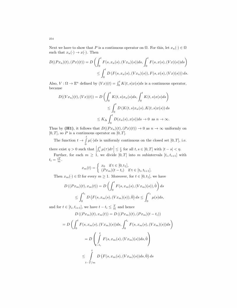
Next we have to show that P is a continuous operator on Ω. For this, let xn(·) ∈ Ωsuch that xn(·)→ x(·). Then
D((Pxn)(t), (Px)(t)) = D
(∫ t
0
F (s, xn(s), (V xn)(s))ds,
∫ t
0
F (s, x(s), (V x)(s))ds
)
≤∫ t
0
D (F (s, xn(s), (V xn)(s)), F (s, x(s), (V x)(s))) ds.
Also, V : Ω→ En defined by (V x)(t) =∫ t
0K(t, s)x(s)ds is a continuous operator,
because
D((V xn)(t), (V x)(t)) = D
(∫ t
0
K(t, s)xn(s)ds,
∫ t
0
K(t, s)x(s)ds
)
≤∫ t
0
D (K(t, s)xn(s),K(t, s)x(s)) ds
≤ K∆
∫ t
0
D(xn(s), x(s))ds→ 0 as n→∞.
Thus by (H1), it follows that D((Pxn)(t), (Px)(t)) → 0 as n → ∞ uniformly on[0, T ], so P is a continuous operator on [0, T ].
The function t →t∫
0
µ(·)ds is uniformly continuous on the closed set [0, T ], i.e.
there exist η > 0 such that∣∣∣∫ tsµ(τ)dτ
∣∣∣ ≤ ε2 for all t, s ∈ [0, T ] with |t− s| < η.
Further, for each m ≥ 1, we divide [0, T ] into m subintervals [ti, ti+1] withti = iT
m .
xm(t) =
x0 if t ∈ [0, t1],(Pxm)(t− ti) if t ∈ [ti, ti+1].
Then xm(·) ∈ Ω for every m ≥ 1. Moreover, for t ∈ [0, t1], we have
D ((Pxm)(t), xm(t)) = D
(∫ t
0
F (s, xm(s), (V xm)(s)), 0
)ds
≤∫ t1
0
D(F (s, xm(s), (V xm)(s)), 0
)ds ≤
∫ t1
0
µ(s)ds,
and for t ∈ [ti, ti+1], we have t− ti ≤ Tm and hence
D ((Pxm)(t), xm(t)) = D ((Pxm)(t), (Pxm)(t− ti))
= D
(∫ t
0
F (s, xm(s), (V xm)(s))ds,
∫ ti
0
F (s, xm(s), (V xm)(s))ds
)
= D
t∫
t−ti
F (s, xm(s), (V xm)(s))ds, 0
≤t∫
t−T/m
D(F (s, xm(s), (V xm)(s))ds, 0
)ds
254
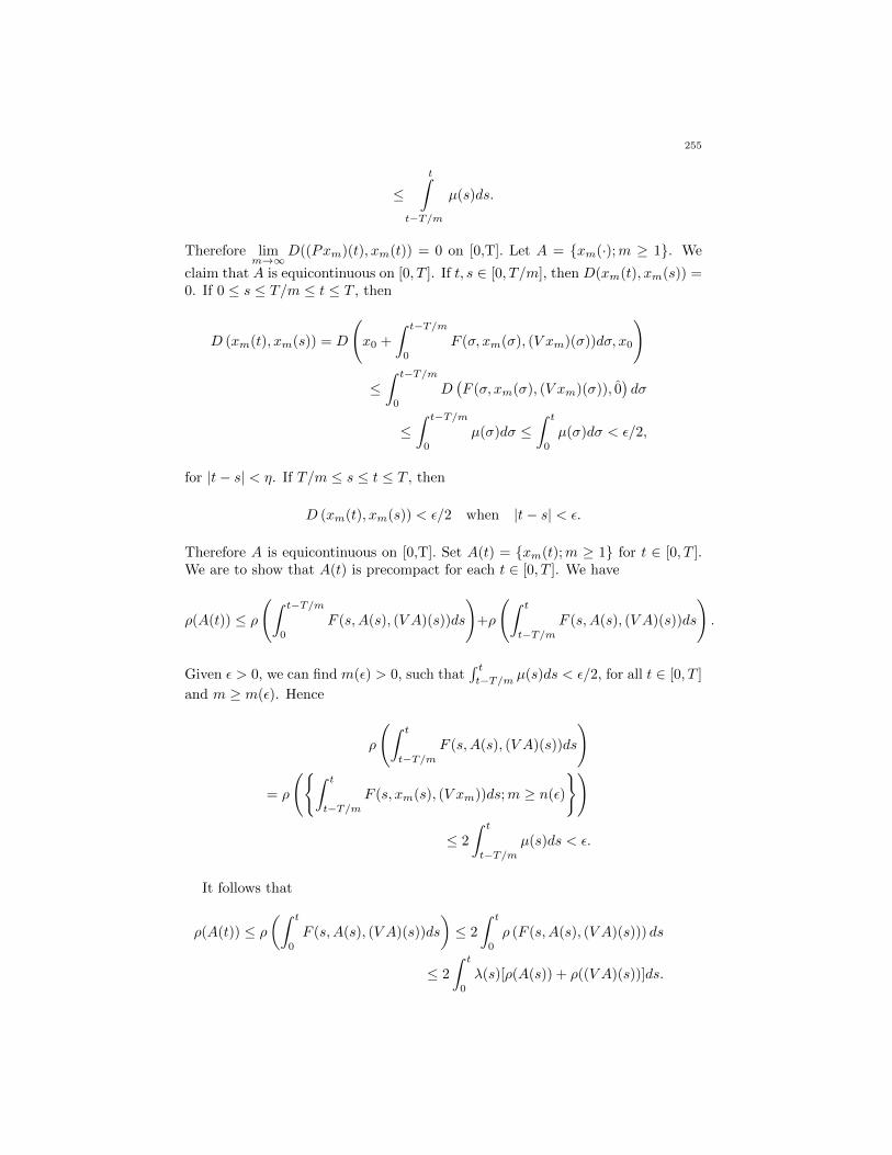
≤t∫
t−T/m
µ(s)ds.
Therefore limm→∞
D((Pxm)(t), xm(t)) = 0 on [0,T]. Let A = xm(·);m ≥ 1. We
claim that A is equicontinuous on [0, T ]. If t, s ∈ [0, T/m], then D(xm(t), xm(s)) =0. If 0 ≤ s ≤ T/m ≤ t ≤ T , then
D (xm(t), xm(s)) = D
(x0 +
∫ t−T/m
0
F (σ, xm(σ), (V xm)(σ))dσ, x0
)
≤∫ t−T/m
0
D(F (σ, xm(σ), (V xm)(σ)), 0
)dσ
≤∫ t−T/m
0
µ(σ)dσ ≤∫ t
0
µ(σ)dσ < ε/2,
for |t− s| < η. If T/m ≤ s ≤ t ≤ T , then
D (xm(t), xm(s)) < ε/2 when |t− s| < ε.
Therefore A is equicontinuous on [0,T]. Set A(t) = xm(t);m ≥ 1 for t ∈ [0, T ].We are to show that A(t) is precompact for each t ∈ [0, T ]. We have
ρ(A(t)) ≤ ρ(∫ t−T/m
0
F (s,A(s), (V A)(s))ds
)+ρ
(∫ t
t−T/mF (s,A(s), (V A)(s))ds
).
Given ε > 0, we can find m(ε) > 0, such that∫ tt−T/m µ(s)ds < ε/2, for all t ∈ [0, T ]
and m ≥ m(ε). Hence
ρ
(∫ t
t−T/mF (s,A(s), (V A)(s))ds
)
= ρ
(∫ t
t−T/mF (s, xm(s), (V xm))ds;m ≥ n(ε)
)
≤ 2
∫ t
t−T/mµ(s)ds < ε.
It follows that
ρ(A(t)) ≤ ρ(∫ t
0
F (s,A(s), (V A)(s))ds
)≤ 2
∫ t
0
ρ (F (s,A(s), (V A)(s))) ds
≤ 2
∫ t
0
λ(s)[ρ(A(s)) + ρ((V A)(s))]ds.
255
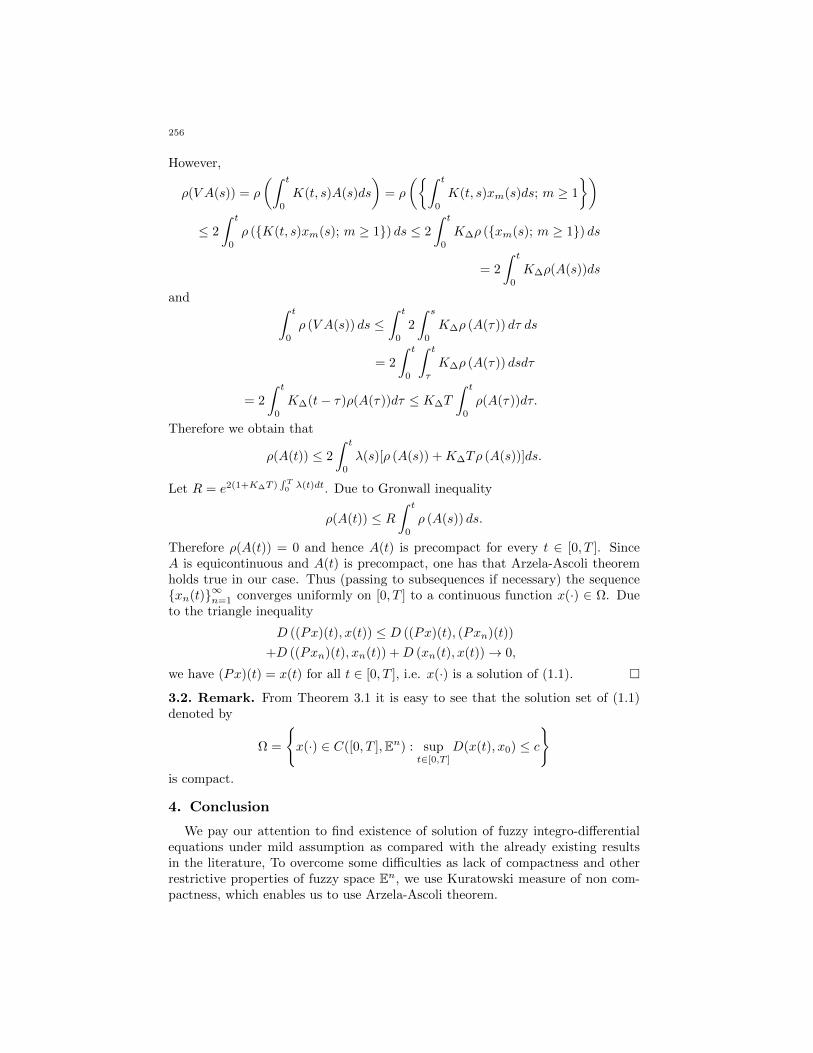
However,
ρ(V A(s)) = ρ
(∫ t
0
K(t, s)A(s)ds
)= ρ
(∫ t
0
K(t, s)xm(s)ds; m ≥ 1
)
≤ 2
∫ t
0
ρ (K(t, s)xm(s); m ≥ 1) ds ≤ 2
∫ t
0
K∆ρ (xm(s); m ≥ 1) ds
= 2
∫ t
0
K∆ρ(A(s))ds
and ∫ t
0
ρ (V A(s)) ds ≤∫ t
0
2
∫ s
0
K∆ρ (A(τ)) dτ ds
= 2
∫ t
0
∫ t
τ
K∆ρ (A(τ)) dsdτ
= 2
∫ t
0
K∆(t− τ)ρ(A(τ))dτ ≤ K∆T
∫ t
0
ρ(A(τ))dτ.
Therefore we obtain that
ρ(A(t)) ≤ 2
∫ t
0
λ(s)[ρ (A(s)) +K∆Tρ (A(s))]ds.
Let R = e2(1+K∆T )∫ T0λ(t)dt. Due to Gronwall inequality
ρ(A(t)) ≤ R∫ t
0
ρ (A(s)) ds.
Therefore ρ(A(t)) = 0 and hence A(t) is precompact for every t ∈ [0, T ]. SinceA is equicontinuous and A(t) is precompact, one has that Arzela-Ascoli theoremholds true in our case. Thus (passing to subsequences if necessary) the sequencexn(t)∞n=1 converges uniformly on [0, T ] to a continuous function x(·) ∈ Ω. Dueto the triangle inequality
D ((Px)(t), x(t)) ≤ D ((Px)(t), (Pxn)(t))
+D ((Pxn)(t), xn(t)) +D (xn(t), x(t))→ 0,
we have (Px)(t) = x(t) for all t ∈ [0, T ], i.e. x(·) is a solution of (1.1). 3.2. Remark. From Theorem 3.1 it is easy to see that the solution set of (1.1)denoted by
Ω =
x(·) ∈ C([0, T ],En) : sup
t∈[0,T ]
D(x(t), x0) ≤ c
is compact.
4. Conclusion
We pay our attention to find existence of solution of fuzzy integro-differentialequations under mild assumption as compared with the already existing resultsin the literature, To overcome some difficulties as lack of compactness and otherrestrictive properties of fuzzy space En, we use Kuratowski measure of non com-pactness, which enables us to use Arzela-Ascoli theorem.
256

Acknowledgement. The research of first Author is partially supported bya grant of the Romanian National Authority for Scientific Research, CNCS UE-FISCDI, project number PN-II-ID-PCE-2011-3-0154, while the research of 2ndAuthor is partially supported by Higher Education Commission, Pakistan.
References
[1] P. Balasubramaniam, M. Chandrasekaran, Existence of solutions of nonlinear Integrodiffer-
ential equation with nonlocal boundary conditions in Banach space, Atti. Sere. Mat. Fis.
Univ. Modena XLVI (1998) 1–13.[2] P. Balasubramaniam, S. Muralisankar, Existence and uniqueness of fuzzy solution for the
nonlinear Fuzzy Integrodifferential equations, Appl. Math. Left. 14 (2001) 455-462.[3] K. Balachandran, P. Prakash, Existence of solutions of nonlinear fuzzy Volterra-Fredholm
integral equations, Indian Journal of Pure Applied Mathematics 33 (2002), 329–343.
[4] J. Banas, B. Rzepka, An application of a measure of noncompactness in the study of As-ymptotic Stability, Applied Mathematical Letters 16 (2003) 1-6.
[5] R. Choudary, T. Donchev, On Peano Theorem for fuzzy differential equations, Fuzzy Sets
and Systems 177 (2011) 93–94.[6] K. Deimling, Multivalued Differential Equations, De Grujter, Berlin, 1992.
[7] O. Kaleva, The Cauchy problem for fuzzy differential equations, Fuzzy Sets and Systems 35
(1990) 389–396.[8] M. Kisielewicz, Multivalued differential equations in separable Banach spaces, J. Opt. The-
ory Appl. 37 (1982) 231–249.
[9] B. Pachpatte, A note on Gronwall-Bellman inequality, J. math. Anal. Appl. 44 (1973) 758-762.
[10] J. Park, H. Han, Existence and uniqueness theorem for a solution of fuzzy Volterra integralequations, Fuzzy Sets and Systems 105 (1999) 481-488.
[11] P. Prakash, V. Kalaiselvi, Fuzzy Voltrerra integral equations with infinite delay, Tamkang
Journal of Mathematics 40 (2009) 19-29,[12] M. Puri, D. Ralescu, Fuzzy random variables, J. Math. Anal. Appl. 114 (1986) 409–422.
[13] H. Romano–Flores, The compactness of E(X), Appl. Math. Lett. 11 (1998) 13–17.
[14] P. Subrahmanyam, S. Sudarsanam, A note on fuzzy Volterra integral equation, Fuzzy Setsand Systems 81 (1996) 237–240.
[15] S. Song, Q. Liu,, Q. Xu, Existence and comparison theorems to Volterra fuzzy integral
equation in (En,D), Fuzzy Sets and Systems 104 (1999), 315–321.
257


Hacettepe Journal of Mathematics and StatisticsVolume 43 (2) (2014), 259 – 277
α-separation axioms based on Lukasiewicz logic
O. R. SAYED a ∗
Abstract
In the present paper, we introduce topological notions defined by meansof α-open sets when these are planted into the framework of Ying’sfuzzifying topological spaces (by Lukasiewicz logic in [0, 1]). We in-troduce Tα
0 −, Tα1 −, Tα
2 (α- Hausdorff)-, Tα3 (α-regular)- and Tα
4 (α-normal)-separation axioms. Furthermore, the Rα
0− and Rα1− separa-
tion axioms are studied and their relations with the Tα1 − and Tα
2 −separation axioms are introduced. Moreover, we clarify the relationsof these axioms with each other as well as the relations with otherfuzzifying separation axioms.
Keywords: Lukasiewicz logic, semantics, fuzzifying topology, fuzzifying separa-tion axioms, α-separation axioms.
2000 AMS Classification: 54A40
1. Introduction and Preliminaries
In the last few years fuzzy topology, as an important research field in fuzzyset theory, has been developed into a quite mature discipline [7-9, 14-15, 27]. Incontrast to classical topology, fuzzy topology is endowed with richer structure,to a certain extent, which is manifested with different ways to generalize certainclassical concepts. So far, according to Ref. [8], the kind of topologies defined byChang [4] and Goguen [5] is called the topologies of fuzzy subsets, and further isnaturally called L-topological spaces if a lattice L of membership values has beenchosen. Loosely speaking, a topology of fuzzy subsets (resp. an L-topologicalspace) is a family τ of fuzzy subsets (resp. L-fuzzy subsets) of nonempty set X,and τ satisfies the basic conditions of classical topologies [11]. On the other hand,Hohle in [6] proposed the terminology L-fuzzy topology to be an L-valued mappingon the traditional powerset P (X) of X. The authors in [10, 23] defined an L-fuzzytopology to be an L-valued mapping on the L-powerset LX of X.
In 1952, Rosser and Turquette [25] proposed emphatically the following prob-lem: If there are many-valued theories beyond the level of predicates calculus,then what are the detail of such theories ? As an attempt to give a partial answer
aDepartment of Mathematics, Faculty of Science, Assiut University, Assiut 71516, EGYPT∗E–mail: o r [email protected]

O. R. SAYED
to this problem in the case of point set topology, Ying in 1991-1993 [28-30] used asemantical method of continuous-valued logic to develop systematically fuzzifyingtopology. Briefly speaking, a fuzzifying topology on a set X assigns each crispsubset of X to a certain degree of being open, other than being definitely openor not. In fact, fuzzifying topologies are a special case of the L-fuzzy topologiesin [10, 23] since all the t-norms on I = [0, 1] are included as a special class oftensor products in these paper. Ying uses one particular tensor product, namely Lukasiewicz conjunction. Thus his fuzzifying topologies are a special class of allthe I - fuzzy topologies considered in the categorical frameworks [10, 23]. Roughlyspeaking, the semantical analysis approach transforms formal statements of in-terest, which are usually expressed as implication formulas in logical language,into some inequalities in the truth value set by truth valuation rules, and thenthese inequalities are demonstrated in an algebraic way and the semantic validityof conclusions is thus established. So far, there has been significant research onfuzzifying topologies [12-13, 20-21, 26]. For example, Shen [26] introduced andstudied T0−, T1−, T2 (Hausdorff)-, T3(regular)- and T4(normal)- separation ax-ioms in fuzzifying topology. In [13], the concepts of the R0− and R1− separationaxioms in fuzzifying topology were added and their relations with the T1− and T2−separation axioms, were studied. Also, in [12] the concepts of fuzzifying α-openset and fuzzifying α-continuity were introduced and studied. In classical topology,α-separation axioms have been studied in [2-3, 16-17, 19, 22]. As well as, theyhave been studied in fuzzy topology in [1,18, 24]. In the present paper, we explorethe problem proposed by Rosser and Turquette [25] in fuzzy α-separation axioms.
A basic structure of the present paper is as follows. First, we offer some def-initions and results which will be needed in this paper. Afterwards, in Section2, in the framework of fuzzifying topology, the concept of α-separation axiomsTα0 −, Tα1 −, Tα2 (α-Hausdorff)-, Tα3 (α-regular)- and Tα4 (α-normal) are discussed.In Section 3, on the bases of fuzzifying topology the Rα0− and Rα1− separation ax-ioms are introduced and their relations with the Tα1 and Tα2−− separation axiomsare studied. Furthermore , we give the relations of these axioms with each other aswell as the relations with other fuzzifying separation axioms. Finally, in a conclu-sion, we summarize the main results obtained and raise some related problems forfurther study. Thus we fill a gap in the existing literature on fuzzifying topology.We will use the terminologies and notations in [12-13, 26, 28, 29] without anyexplanation. We will use the symbol ⊗ instead of the second ”AND” operation ∧
·as dot is hardly visible. This mean that [α] ≤ [ϕ→ ψ]⇔ [α]⊗ [ϕ] ≤ [ψ].A fuzzifying topology on a set X [6, 28] is a mapping τ ∈ =(P (X)) such that:
(1) τ(X) = 1, τ(φ) = 1;(2) for any A,B, τ(A ∩B) ≥ τ(A) ∧ τ(B);
(3) for any Aλ : λ ∈ Λ, τ( ⋃λ∈Λ
Aλ
)≥ ∧λ∈Λ
τ (Aλ) .
The family of all fuzzifying α-open sets [12], denoted by τα ∈ =(P (X)), is definedasA ∈ τα := ∀x(x ∈ A→ x ∈ Int(Cl(Int(A)))), i. e., τα(A) =
∧x∈A
Int(Cl(Int(A)))(x)
The family of all fuzzifying α-closed sets [12], denoted by Fα ∈ =(P (X)), is definedas A ∈ Fα := X−A ∈ τα. The fuzzifying α-neighborhood system of a point x ∈ X
260

α- separation axioms based on Lukasiewicz logic
[12] is denoted by Nαx ∈ =(P (X)) and defined as Nα
x (A) =∨
x∈B⊆Aτα(B).The
fuzzifying α-closure of a set A ⊆ X [12], denoted by Clα ∈ =(X), is defined asClα(A)(x) = 1−Nα
x (X −A).Let (X, τ) be a fuzzifying topological space. The binary fuzzy predicatesK,H,M ∈=(X×X), V ∈ =(X×P (X)) and W ∈ =(P (X)×P (X)) [13] are defined as follows:
(1) K(x, y) := ∃A((A ∈ Nx ∧ y /∈ A) ∨ (A ∈ Ny ∧ x /∈ A));(2) H(x, y) := ∃B∃C((B ∈ Nx ∧ y /∈ B) ∧ (C ∈ Ny ∧ x /∈ C));(3) M(x, y) := ∃B∃C(B ∈ Nx ∧ C ∈ Ny ∧B ∩ C ≡ ∅);(4) V (x,D) := ∃A∃B(A ∈ Nx ∧B ∈ τ ∧D ⊆ B ∧A ∩B ≡ ∅);(5) W (A,B) := ∃G∃H(G ∈ τ ∧H ∈ τ ∧A ⊆ G ∧B ⊆ H ∧G ∩H ≡ ∅).
Let Ω be the class of all fuzzifying topological spaces. The unary fuzzy predicatesTi ∈ =(Ω), i = 0, 1, 2, 3, 4 [26] (see the rewritten form in [13]) and Ri ∈ =(Ω), i =0, 1 [13] are defined as follows:
(1) (X, τ) ∈ T0 := ∀x∀y(x ∈ X ∧ y ∈ X ∧ x 6= y) −→ K(x, y);(2) (X, τ) ∈ T1 := ∀x∀y(x ∈ X ∧ y ∈ X ∧ x 6= y) −→ H(x, y);(3) (X, τ) ∈ T2 := ∀x∀y(x ∈ X ∧ y ∈ X ∧ x 6= y) −→M(x, y);(4) (X, τ) ∈ T3 := ∀x∀D(x ∈ X ∧D ∈ F ∧ x /∈ D) −→ V (x,D);(5) (X, τ) ∈ T4 := ∀A∀B(A ∈ F ∧B ∈ F ∧A ∩B = ∅) −→W (A,B);(6) (X, τ) ∈ R0 := ∀x∀y(x ∈ X ∧ y ∈ X ∧ x 6= y) −→ (K(x, y) −→ H(x, y));(7) (X, τ) ∈ R1 := ∀x∀y(x ∈ X ∧ y ∈ X ∧ x 6= y) −→ (K(x, y) −→M(x, y)).
2. Fuzzifying α- separation axioms and their equivalents
For simplicity we give the following definition.
2.1. Definition. Let (X, τ) be a fuzzifying topological space. The binary fuzzypredicates Kα, Hα,Mα ∈ =(X × X), V α ∈ =(X × P (X)) and Wα ∈ =(P (X) ×P (X)) are defined as follows:
(1) Kα(x, y) := ∃A((A ∈ Nαx ∧ y /∈ A) ∨ (A ∈ Nα
y ∧ x /∈ A));(2) Hα(x, y) := ∃B∃C((B ∈ Nα
x ∧ y /∈ B) ∧ (C ∈ Nαy ∧ x /∈ C));
(3) Mα(x, y) := ∃B∃C(B ∈ Nαx ∧ C ∈ Nα
y ∧B ∩ C ≡ ∅);(4) V α(x,D) := ∃A∃B(A ∈ Nα
x ∧B ∈ τα ∧D ⊆ B ∧A ∩B ≡ ∅);(5) Wα(A,B) := ∃G∃H(G ∈ τα ∧H ∈ τα ∧A ⊆ G ∧B ⊆ H ∧G ∩H ≡ ∅).
2.2. Definition. Let Ω be the class of all fuzzifying topological spaces. The unaryfuzzy predicates Tαi ∈ =(Ω), i = 0, 1, 2, 3, 4 and Rαi ∈ =(Ω), i = 0, 1 are defined asfollows:
(1) (X, τ) ∈ Tα0 := ∀x∀y(x ∈ X ∧ y ∈ X ∧ x 6= y) −→ Kα(x, y);(2) (X, τ) ∈ Tα1 := ∀x∀y(x ∈ X ∧ y ∈ X ∧ x 6= y) −→ Hα(x, y);(3) (X, τ) ∈ Tα2 := ∀x∀y(x ∈ X ∧ y ∈ X ∧ x 6= y) −→Mα(x, y);(4) (X, τ) ∈ Tα3 := ∀x∀D(x ∈ X ∧D ∈ F ∧ x /∈ D) −→ V α(x,D);(5) (X, τ) ∈ Tα4 := ∀A∀B(A ∈ F ∧B ∈ F ∧A ∩B = ∅) −→Wα(A,B);
(6) (X, τ) ∈ Tα′3 := ∀x∀D(x ∈ X ∧D ∈ Fα ∧ x /∈ D) −→ V (x,D);
(7) (X, τ) ∈ Tα′4 := ∀A∀B(A ∈ Fα ∧B ∈ Fα ∧A ∩B = ∅) −→W (A,B);(8) (X, τ) ∈ Rα0 := ∀x∀y(x ∈ X ∧ y ∈ X ∧ x 6= y) −→ (Kα(x, y) −→ Hα(x, y));(9) (X, τ) ∈ Rα1 := ∀x∀y(x ∈ X ∧ y ∈ X ∧ x 6= y) −→ (Kα(x, y) −→Mα(x, y)).
2.3. Theorem. Let (X, τ) be a fuzzifying topological space. Then we have
261

O. R. SAYED
|= (X, τ) ∈ Tα0 ←→ ∀x∀y(x ∈ X ∧ y ∈ X ∧x 6= y −→ (¬(x ∈ Clα(y))∨¬(y ∈Clα(x)))).
Proof. Since for any x,A,B, |= A ⊆ B → (A ∈ Nαx → B ∈ Nα
x ) (see [12, Theorem4.2 (2)]), we have
[(X, τ) ∈ Tα0 ] =∧
x 6=ymax(
∨
y/∈ANαx (A),
∨
x/∈ANαy (A))
=∧
x 6=ymax(Nα
x (X − y), Nαy (X − x))
=∧
x 6=ymax(1− Clα(y)(x), 1− Clα(x)(y))
=∧
x 6=y(¬(Clα(y)(x)) ∨ ¬(Clα(x)(y)))
= [∀x∀y(x ∈ X ∧ y ∈ X ∧ x 6= y −→ (¬(x ∈ Clα(y)) ∨ ¬(y ∈ Clα(x))))].
2.4. Theorem. For any fuzzifying topological space (X, τ) we have|= ∀x(x ∈ Fα)↔ (X, τ) ∈ Tα1 .
Proof. Since τα(A) =∧x∈A
Nαx (A) (Corollary 4.1 in [12]), for any x1, x2 with x1 6=
x2, we have
[∀x(x ∈ Fα)] =∧
x∈XFα(x) =
∧
x∈Xτα(X − x) ≤
∧
x∈X
∧
y∈X−xNαy (X − x)
≤∧
y∈X−x2Nαy (X − x2) ≤ Nα
x1(X − x2) =
∨
x2 /∈ANαx1
(A).
Similarly, we have, [∀x(x ∈ Fα)] ≤ ∨x1 /∈B
Nαx2
(B). Then
[∀x(x ∈ Fα)] ≤∧
x1 6=x2
min(∨
x2 /∈ANαx1
(A),∨
x1 /∈BNαx2
(B))
=∧
x1 6=x2
∨
x1 /∈B, x2 /∈Amin(Nα
x1(A), Nα
x2(B))
= [(X, τ) ∈ Tα1 ].
262

α- separation axioms based on Lukasiewicz logic
On the other hand
[(X, τ) ∈ Tα1 ] =∧
x1 6=x2
min(∨
x2 /∈ANαx1
(A),∨
x1 /∈BNαx2
(B))
=∧
x1 6=x2
min(Nαx1
(X − x2), Nαx2
(X − x1))
≤∧
x1 6=x2
Nαx1
(X − x2) =∧
x2∈X
∧
x1∈X−x2Nαx1
(X − x2)
=∧
x2∈Xτα(X − x2) =
∧
x∈Xτα(X − x)
= [∀x(x ∈ Fα)].
Therefore [∀x(x ∈ Fα)] = [(X, τ) ∈ Tα1 ].
2.5. Definition. Let (X, τ) be a fuzzifying topological space. The fuzzifying α-derived set Dα(A) of A is defined as follows: x ∈ Dα(A) := ∀B(B ∈ Nα
x →B ∩ (A− x) 6= φ).
2.6. Lemma. Dα(A)(x) = 1−Nαx ((X −A) ∪ x).
Proof. From Theorem 4.2 (2) [12] we have
Dα(A)(x) = 1−∨
B∩(A−x)=φNαx (B) = 1−Nα
x ((X −A) ∪ x).
2.7. Theorem. For any finite set A ⊆ X, |= Tα1 (X, τ)→ Dα(A) ≡ φ.
Proof. From Theorem 4.2 (2) [12] we have
∧
y∈X−ANαy ((X −A) ∪ y) ≥
∧
y∈X−ANαy (X −A) =
∧
y∈X−ANαy (⋂
x∈A(X − x)
≥∧
y∈X−A
∧
x∈ANαy (X − x) ≥
∧
x 6=yNαy (X − x).
Also
∧
y∈ANαy ((X −A) ∪ y) =
∧
y∈ANαy (X − (A− y)) =
∧
y∈ANαy (
⋂
x∈A−y(X − x)
≥∧
y∈A
∧
x∈A−yNαy (X − x) ≥
∧
x6=yNαy (X − x).
263

O. R. SAYED
Therefore
[Dα(A) ≡ φ] =∧
x∈XNαx ((X −A) ∪ x)
= min(∧
y∈X−ANαy ((X −A) ∪ y),
∧
y∈ANαy ((X −A) ∪ y))
≥∧
x6=yNαy (X − x) =
∧
x∈X
∧
x∈X−yNαy (X − x)
=∧
x∈Xτα(X − x) =
∧
x∈XFα(x) = Tα1 (X, τ).
2.8. Definition. The fuzzifying α-local basis βαx of x is a function from P (X)into I = [0, 1] satisfying the following conditions:
(1) |= βαx ⊆ Nαx , and (2) |= A ∈ Nα
x −→ ∃B(B ∈ βαx ∧ x ∈ B ⊆ A).
2.9. Lemma. |= A ∈ Nαx ←→ ∃B(B ∈ βαx ∧ x ∈ B ⊆ A).
Proof. From condition (1) in Definition 2.8 and Theorem 4.2 (2) in [12] we haveNαx (A) ≥ Nα
x (B) ≥ βαx (B) for each B ∈ P (X) such that x ∈ B ⊆ A. So Nαx (A) ≥∨
x∈B⊆Aβαx (B). From condition (2) in Definition 2.8 we have Nα
x (A) ≤ ∨x∈B⊆A
βαx (B).
Hence Nαx (A) =
∨x∈B⊆A
βαx (B).
2.10. Theorem. If βαx is a fuzzifying α-local basis of x, then|= (X, τ) ∈ Tα1 ←→ ∀x∀y(x ∈ X ∧ y ∈ X ∧ x 6= y −→ ∃A(A ∈ βαx ∧ y /∈ A)).
Proof. For any x, y with x 6= y,∨y/∈A
βαx (A) ≤ ∨y/∈A
Nαx (A),
∨x/∈B
βαy (B) ≤ ∨x/∈B
Nαy (B).
So min(∨y/∈A
βαx (A),∨x/∈B
βαy (B)) ≤ min(∨y/∈A
Nαx (A),
∨x/∈B
Nαy (B)) =
∨y/∈A,x/∈B
min(Nαx (A), Nα
y (B)),
i.e.,∧x 6=y
∨y/∈A
βαx (A) ≤ ∧x 6=y
∨y/∈A,x/∈B
min(Nαx (A), Nα
y (B)) = [(X, τ) ∈ Tα1 ]. On the
other hand, for any B with x ∈ B ⊆ X − y we have y /∈ B. So∨y/∈A
βαx (A) ≥
βαx (B). According to Definition 2.8 we have∨y/∈A
βαx (A) ≥ ∨x∈B⊆X−y
βαx (B) =
Nαx (X − y). Furthermore, from Corollary 4.1 [12] we have
∧x6=y
∨y/∈A
βαx (A) ≥∧x6=y
Nx(X−y) =∧y∈X
∧x∈X−y
Nx(X−y) =∧y∈X
τα(X−y) =∧y∈X
Fα(y) =
[(X, τ) ∈ Tα1 ].
2.11. Theorem. If βαx is a fuzzifying α-local basis of x, then|= (X, τ) ∈ Tα2 ←→ ∀x∀y(x ∈ X ∧ y ∈ X ∧ x 6= y −→ ∃B(B ∈ βαx ∧ y ∈
¬(Clα(B)))).
264

α- separation axioms based on Lukasiewicz logic
Proof.
[∀x∀y(x ∈ X ∧ y ∈ X ∧ x 6= y −→ ∃B(B ∈ βαx ∧ y ∈ ¬(Clα(B))))]
=∧
x 6=y
∨
B∈P (X)
min(βαx (B),¬(1−Nαy (X −B)))
=∧
x 6=y
∨
B∈P (X)
min(βαx (B), Nαy (X −B))
=∧
x 6=y
∨
B∈P (X)
∨
y∈C⊆X−Bmin(βαx (B), βαy (C))
=∧
x 6=y
∨
B∩C=∅
∨
x∈D⊆B, y∈E⊆Cmin(βαx (D), βαy (E))
=∧
x 6=y
∨
B∩C=∅min(
∨
x∈D⊆Bβαx (D),
∨
y∈E⊆Cβαy (E))
=∧
x 6=y
∨
B∩C=∅min(Nα
x (B), Nαy (C)) = [(X, τ) ∈ Tα2 ].
2.12. Definition. The binary fuzzy predicate α ∈ =(N(X)×X), is defined asSα x := ∀A(A ∈ Nα
x −→ S ⊂∼ A), where N(X) is the set of all nets of X, [Sα x]stands for the degree to which S α-converges to x and ” ⊂∼ ” is the binary crisppredicates ”almost in ”.
2.13. Theorem. Let (X, τ) be a fuzzifying topological space and S ∈ N(X).|= (X, τ) ∈ Tα2 ←→ ∀S∀x∀y((S ⊆ X)∧(x ∈ X)∧(y ∈ X)∧(Sαx)∧(Sα y) −→x = y).
Proof. [(X, τ) ∈ Tα2 ] =∧x 6=y
∨A∩B=∅
(Nαx (A) ∧Nα
y (B)),
[∀S∀x∀y((S ⊆ X) ∧ (x ∈ X) ∧ (y ∈ X) ∧ (S α x) ∧ (S α y) −→ x = y)]=∧x6=y
∧S⊆X
(∨
S 6⊂∼ ANαx (A) ∨ ∨
S 6⊂∼ BNαy (B))
=∧x6=y
∧S⊆X
∨S 6⊂∼ A
∨S 6⊂∼ B
(Nαx (A) ∨Nα
y (B)).
(1) If A∩B = ∅, then for any S ∈ N(X), we have S 6 ⊂∼ A or S 6 ⊂∼ B. Therefore,we obtain Nα
x (A) ∧Nαy (B) ≤ ∨
S 6⊂∼ ANαx (A) or Nα
x (A) ∧Nαy (B) ≤ ∨
S 6⊂∼ BNαx (B).
Consequently,∨
A∩B=∅(Nα
x (A) ∧Nαy (B)) ≤ ∧
S⊆X(∨
S 6⊂∼ ANαx (A) ∨ ∨
S 6⊂∼ BNαy (B)),
and[(X, τ) ∈ Tα2 ] ≤ [∀S∀x∀y((S ⊆ X) ∧ (x ∈ X) ∧ (y ∈ X) ∧ (S α x) ∧ (S α y) →x = y)].
(2) First, for any x, y with x 6= y, if∨
A∩B=∅(Nα
x (A)∧Nαy (B)) < t, then Nα
x (A) <
t or Nαy (B) < t provided A∩B = ∅, i.e., A∩B 6= ∅ when A ∈ (Nα
x )t and B ∈ (Nαy )t.
Now, set a net S∗ : (Nαx )t × (Nα
y )t −→ X, (A,B) 7−→ x(A,B) ∈ A ∩ B. Then forany A ∈ (Nα
x )t, B ∈ (Nαy )t, we have S∗⊂∼ A and S∗⊂∼ B. Therefore, if S∗ 6 ⊂∼ A and
265

O. R. SAYED
S∗ 6 ⊂∼ B, then A /∈ (Nαx )t, B /∈ (Nα
y )t, i.e., Nαx (A) ∨ Nα
y (B)) < t. Consequently∨S∗ 6⊂∼ A
∨S∗ 6⊂∼ B
(Nαx (A)∨Nα
y (B)) ≤ t. Moreover∧S⊆X
∨S 6⊂∼ A
∨S 6⊂∼ B
(Nαx (A)∨Nα
y (B)) ≤ t.
Second, for any positive integer i, there exists xi, yi with xi 6= yi, and∨
A∩B=∅(Nα
xi(A) ∧Nαyi(B)) < [(X, τ) ∈ Tα2 ] + 1/i,
and hence∧
S⊆X
∨
S 6⊂∼ A
∨
S 6⊂∼ B(Nα
xi(A) ∨Nαyi(B)) < [(X, τ) ∈ Tα2 ] + 1/i.
So we have
[∀S∀x∀y((S ⊆ X) ∧ (x ∈ X) ∧ (y ∈ X) ∧ (S α x) ∧ (S α y) −→ x = y)]
=∧
x 6=y
∧
S⊆X
∨
S 6⊂∼ A
∨
S 6⊂∼ B(Nα
x (A) ∨Nαy (B)) ≤ [(X, τ) ∈ Tα2 ].
2.14. Lemma. Let (X, τ) be a fuzzifying topological space.(1) If D ⊆ B, then
∨A∩B=∅
Nαx (A) =
∨A∩B=∅, D⊆B
Nαx (A),
(2)∨
A∩B=∅
∧y∈D
Nαy (X −A) =
∨A∩B=∅, D⊆B
τα(B).
Proof. (1) Since D ⊆ B then∨
A∩B=∅Nαx (A) =
∨
A∩B=∅Nαx (A)∧[D ⊆ B] =
∨
A∩B=∅, D⊆BNαx (A).
(2) Let y ∈ D and A ∩B = ∅. Then∨
A∩B=∅, D⊆Bτα(B) =
∨
A∩B=∅, D⊆Bτα(B) ∧ [y ∈ D]
=∨
y∈D⊆B⊆X−Aτα(B) =
∨
y∈B⊆X−Aτα(B)
= Nαy (X −A) =
∧
y∈DNαy (X −A)
=∨
A∩B=∅
∧
y∈DNαy (X −A).
2.15. Definition. Let (X, τ) be a fuzzifying topological space.
αT(1)3 (X, τ) := ∀x∀D(x ∈ X∧D ∈ F∧x /∈ D −→ ∃A(A ∈ Nα
x ∧(D ⊆ X−Clα(A)))).
2.16. Theorem. |= (X, τ) ∈ Tα3 ←→ (X, τ) ∈ αT (1)3 .
266

α- separation axioms based on Lukasiewicz logic
Proof.
αT(1)3 (X, τ) =
∧
x/∈Dmin(1, 1− τ(X −D) +
∨
A∈P (X)
min(Nαx (A),
∧
y∈D(1− Clα(A)(y))))
=∧
x/∈Dmin(1, 1− τ(X −D) +
∨
A∈P (X)
min(Nαx (A),
∧
y∈DNαy (X −A)))
and Tα3 (X, τ) =∧
x/∈Dmin(1, 1− τ(X −D) +
∨
A∩B=∅, D⊆Bmin(Nα
x (A), τα(B))).
So, the result holds if we prove that∨
A∈P (X)
min(Nαx (A),
∧
y∈DNαy (X −A)) =
∨
A∩B=∅, D⊆Bmin(Nα
x (A), τα(B)) (∗)
It is clear that, on the left-hand side of (∗) in the case of A∩D 6= ∅ there existsy ∈ X such that y ∈ D and y /∈ X − A. So,
∧y∈D
Nαy (X − A) = 0 and thus (∗)
becomes
∨
A∈P (X), A∩B=∅min(Nα
x (A),∧
y∈DNαy (X −A)) =
∨
A∩B=∅, D⊆Bmin(Nα
x (A), τα(B)),
which is obtained from Lemma 2.14.
2.17. Definition. Let (X, τ) be a fuzzifying topological space.
αT(2)3 (X, τ) := ∀x∀B(x ∈ B ∧B ∈ τ −→ ∃A(A ∈ Nα
x ∧ Clα(A) ⊆ B)).
2.18. Theorem. |= (X, τ) ∈ Tα3 ←→ (X, τ) ∈ αT (2)3 .
Proof. From Theorem 2.16 we have
Tα3 (X, τ) =∧
x/∈Dmin(1, 1−τ(X−D)+
∨
A∈P (X)
min(Nαx (A),
∧
y∈DNαy (X−A))).
Now,
αT(2)3 (X, τ) =
∧
x∈Bmin(1, 1− τ(B) +
∨
A∈P (X)
min(Nαx (A),
∧
y∈X−B(1− Clα(A)(y))))
=∧
x∈Bmin(1, 1− τ(B) +
∨
A∈P (X)
min(Nαx (A),
∧
y∈X−B(1− (1−Nα
y (X −A)))))
=∧
x∈Bmin(1, 1− τ(B) +
∨
A∈P (X)
min(Nαx (A),
∧
y∈X−BNαy (X −A))).
Put B = X −D we have
αT(2)3 (X, τ) =
∧
x/∈Dmin(1, 1− τ(X −D) +
∨
A∈P (X)
min(Nαx (A),
∧
y∈DNαy (X −A)))
= Tα3 (X, τ).
267
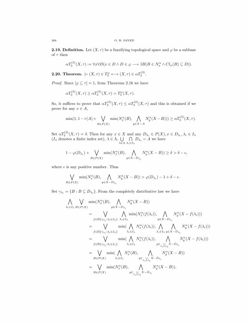
O. R. SAYED
2.19. Definition. Let (X, τ) be a fuzzifying topological space and ϕ be a subbaseof τ then
αT(3)3 (X, τ) := ∀x∀D(x ∈ D ∧D ∈ ϕ −→ ∃B(B ∈ Nα
x ∧ Clα(B) ⊆ D)).
2.20. Theorem. |= (X, τ) ∈ Tα3 ←→ (X, τ) ∈ αT (3)3 .
Proof. Since [ϕ ⊆ τ ] = 1, from Theorems 2.16 we have
αT(3)3 (X, τ) ≥ αT (2)
3 (X, τ) = Tα3 (X, τ).
So, it suffices to prove that αT(3)3 (X, τ) ≤ αT
(2)3 (X, τ) and this is obtained if we
prove for any x ∈ A,
min(1, 1− τ(A)+∨
B∈P (X)
min(Nαx (B),
∧
y∈X−ANαy (X−B))) ≥ αT (3)
3 (X, τ).
Set αT(3)3 (X, τ) = δ. Then for any x ∈ X and any Dλi ∈ P (X), x ∈ Dλi , λi ∈ Iλ
(Iλ denotes a finite index set), λ ∈ Λ,⋃λ∈Λ
⋂λi∈Iλ
Dλi = A we have
1− ϕ(Dλi) +∨
B∈P (X)
min(Nαx (B),
∧
y∈X−Dλi
Nαy (X −B)) ≥ δ > δ − ε,
where ε is any positive number. Thus
∨
B∈P (X)
min(Nαx (B),
∧
y∈X−Dλi
Nαy (X −B)) > ϕ(Dλi)− 1 + δ − ε.
Set γλi = B : B ⊆ Dλi. From the completely distributive law we have
∧
λi∈Iλ
∨
B∈P (X)
min(Nαx (B),
∧
y∈X−Dλi
Nαy (X −B))
=∨
f∈Πγλi :λi∈Iλ
∧
λi∈Iλmin(Nα
x (f(λi)),∧
y∈X−Dλi
Nαy (X − f(λi)))
=∨
f∈Πγλi :λi∈Iλmin(
∧
λi∈IλNαx (f(λi)),
∧
λi∈Iλ
∧
y∈X−Dλi
Nαy (X − f(λi)))
=∨
f∈Πγλi :λi∈Iλmin(
∧
λi∈IλNαx (f(λi)),
∧
y∈ ∪λi∈Iλ
X−Dλi
Nαy (X − f(λi)))
=∨
B∈P (X)
min(∧
λi∈IλNαx (B),
∧
y∈ ∪λi∈Iλ
X−Dλi
Nαy (X −B))
=∨
B∈P (X)
min(Nαx (B),
∧
y∈ ∪λi∈Iλ
X−Dλi
Nαy (X −B)),
268

α- separation axioms based on Lukasiewicz logic
where B = f(λi).Similarly, we can prove
∧
λ∈Λ
∨
B∈P (X)
min(Nαx (B),
∧
y∈ ∪λi∈Iλ
X−Dλi
Nαy (X −B))
=∨
B∈P (X)
min(Nαx (B),
∧
y∈ ∪λ∈Λ
∪λi∈Iλ
X−Dλi
Nαy (X −B))
≤∨
B∈P (X)
min(Nαx (B),
∧
y∈ ∩λ∈Λ
∪λi∈Iλ
X−Dλi
Nαy (X −B))
≤∨
B∈P (X)
min(Nαx (B),
∧
y∈X−ANαy (X −B)),
so we have∨
B∈P (X)
min(Nαx (B),
∧
y∈X−ANαy (X −B))
≥∧
λ∈Λ
∧
λi∈Iλ
∨
B∈P (X)
min(Nαx (B),
∧
y∈X−Dλi
Nαy (X −B))
≥∧
λ∈Λ
∧
λi∈Iλϕ(Dλi)− 1 + δ − ε.
For any Iλ and Λ that satisfy⋃λ∈Λ
⋂λi∈Iλ
Dλi = A the above inequality is true. So,
∨
B∈P (X)
min(Nαx (B),
∧
y∈X−ANαy (X −B))
≥∨
∪λ∈ΛDλ=A
∧
λ∈Λ
∨
∩λi∈IλDλi=Dλ
∧
λi∈Iλϕ(Dλi)− 1 + δ − ε
= τ(A)− 1 + δ − ε.
i.e., min(1, 1−τ(A)+∨
B∈P (X)
min(Nαx (B),
∧
y∈X−ANαy (X−B))) ≥ δ−ε.
Because ε is any arbitrary positive number, when ε −→ 0 we have
αT(2)3 (X, τ) ≥ δ = αT
(3)3 (X, τ). So, |= (X, τ) ∈ Tα3 ←→ (X, τ) ∈ αT (3)
3 .
2.21. Definition. Let (X, τ) be any fuzzifying topological space.
(1) α′T (1)3 (X, τ) := ∀x∀D(x ∈ X ∧ D ∈ Fα ∧ x /∈ D −→ ∃A(A ∈ Nx ∧ (D ⊆
X − Cl(A))));
(2) α′T (2)3 (X, τ) := ∀x∀B(x ∈ B ∧B ∈ τα −→ ∃A(A ∈ Nx ∧ Cl(A) ⊆ B));
(3) αT(1)4 (X, τ) := ∀A∀B(A ∈ τ ∧ B ∈ F ∧ A ∩ B ≡ ∅ → ∃G(G ∈ τ ∧ A ⊆
G ∧ Clα(G) ∩B ≡ φ));
(4) αT(2)4 (X, τ) := ∀A∀B(A ∈ F∧B ∈ τ∧A ⊆ B → ∃G(G ∈ τ∧A ⊆ G∧Clα(G) ⊆
B));
(5) α′T (1)4 (X, τ) := ∀A∀B(A ∈ τ ∧ B ∈ Fα ∧ A ∩ B ≡ ∅ → ∃G(G ∈ τ ∧ A ⊆
G ∧ Cl(G) ∩B ≡ φ));
269
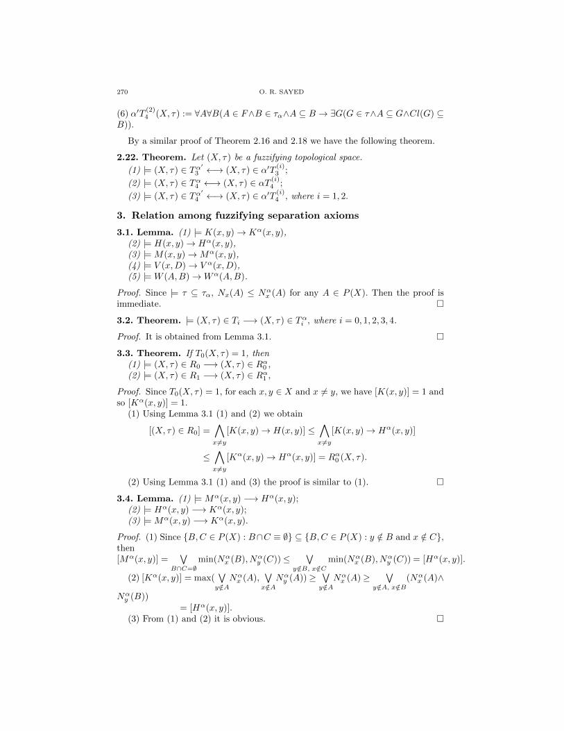
O. R. SAYED
(6) α′T (2)4 (X, τ) := ∀A∀B(A ∈ F∧B ∈ τα∧A ⊆ B → ∃G(G ∈ τ∧A ⊆ G∧Cl(G) ⊆
B)).
By a similar proof of Theorem 2.16 and 2.18 we have the following theorem.
2.22. Theorem. Let (X, τ) be a fuzzifying topological space.
(1) |= (X, τ) ∈ Tα′3 ←→ (X, τ) ∈ α′T (i)3 ;
(2) |= (X, τ) ∈ Tα4 ←→ (X, τ) ∈ αT (i)4 ;
(3) |= (X, τ) ∈ Tα′4 ←→ (X, τ) ∈ α′T (i)4 , where i = 1, 2.
3. Relation among fuzzifying separation axioms
3.1. Lemma. (1) |= K(x, y)→ Kα(x, y),(2) |= H(x, y)→ Hα(x, y),(3) |= M(x, y)→Mα(x, y),(4) |= V (x,D)→ V α(x,D),(5) |= W (A,B)→Wα(A,B).
Proof. Since |= τ ⊆ τα, Nx(A) ≤ Nαx (A) for any A ∈ P (X). Then the proof is
immediate. 3.2. Theorem. |= (X, τ) ∈ Ti −→ (X, τ) ∈ Tαi , where i = 0, 1, 2, 3, 4.
Proof. It is obtained from Lemma 3.1. 3.3. Theorem. If T0(X, τ) = 1, then
(1) |= (X, τ) ∈ R0 −→ (X, τ) ∈ Rα0 ,(2) |= (X, τ) ∈ R1 −→ (X, τ) ∈ Rα1 ,
Proof. Since T0(X, τ) = 1, for each x, y ∈ X and x 6= y, we have [K(x, y)] = 1 andso [Kα(x, y)] = 1.
(1) Using Lemma 3.1 (1) and (2) we obtain
[(X, τ) ∈ R0] =∧
x 6=y[K(x, y)→ H(x, y)] ≤
∧
x6=y[K(x, y)→ Hα(x, y)]
≤∧
x 6=y[Kα(x, y)→ Hα(x, y)] = Rα0 (X, τ).
(2) Using Lemma 3.1 (1) and (3) the proof is similar to (1). 3.4. Lemma. (1) |= Mα(x, y) −→ Hα(x, y);
(2) |= Hα(x, y) −→ Kα(x, y);(3) |= Mα(x, y) −→ Kα(x, y).
Proof. (1) Since B,C ∈ P (X) : B∩C ≡ ∅ ⊆ B,C ∈ P (X) : y /∈ B and x /∈ C,then[Mα(x, y)] =
∨B∩C=∅
min(Nαx (B), Nα
y (C))≤ ∨y/∈B, x/∈C
min(Nαx (B), Nα
y (C)) = [Hα(x, y)].
(2) [Kα(x, y)] = max(∨y/∈A
Nαx (A),
∨x/∈A
Nαy (A))≥ ∨
y/∈ANαx (A)≥ ∨
y/∈A, x/∈B(Nα
x (A)∧
Nαy (B))
= [Hα(x, y)].(3) From (1) and (2) it is obvious.
270

α- separation axioms based on Lukasiewicz logic
3.5. Theorem. Let (X, τ) be a fuzzifying topological space. Then we have(1) |= (X, τ) ∈ Tα1 −→ (X, τ) ∈ Tα0 ;(2) |= (X, τ) ∈ Tα2 −→ (X, τ) ∈ Tα1 ;(3) |= (X, τ) ∈ Tα2 −→ (X, τ) ∈ Tα0 .
Proof. The proof of (1) and (2) are obtained from Lemma 3.4 (2) and (1), respec-tively.
(3) From (1) and (2) above the result is obtained.
3.6. Theorem. |= (X, τ) ∈ Rα1 −→ (X, τ) ∈ Rα0 .
Proof. From Lemma 3.4 (2), the proof is immediate.
3.7. Theorem. For any fuzzifying topological space (X, τ) we have(1) |= (X, τ) ∈ Tα1 −→ (X, τ) ∈ Rα0 ;(2) |= (X, τ) ∈ Tα1 −→ (X, τ) ∈ Rα0 ∧ (X, τ) ∈ Tα0 ;(3) If Tα0 (X, τ) = 1, then |= (X, τ) ∈ Tα1 ←→ (X, τ) ∈ Rα0 ∧ (X, τ) ∈ Tα0 .
Proof. (1) Tα1 (X, τ) =∧x6=y[Hα(x, y)] ≤ ∧x 6=y[Kα(x, y) −→ Hα(x, y)] = Rα0 (X, τ).
(2) It is obtained from (1) and from Theorem 3.5 (1).(3) Since Tα0 (X, τ) = 1, for every x, y ∈ X such that x 6= y, then we have
[Kα(x, y)] = 1. Therefore
[(X, τ) ∈ Rα0 ∧ (X, τ) ∈ Tα0 ] = [(X, τ) ∈ Rα0 ]
=∧
x 6=ymin(1, 1− [Kα(x, y)] + [Hα(x, y)])
=∧
x 6=y[Hα(x, y)] = Tα1 (X, τ).
3.8. Theorem. Let (X, τ) be a fuzzifying topological space.(1) |= (X, τ) ∈ Rα0 ⊗ (X, τ) ∈ Tα0 −→ (X, τ) ∈ Tα1 , and(2) If Tα0 (X, τ) = 1, then |= (X, τ) ∈ Rα0 ⊗ (X, τ) ∈ Tα0 ←→ (X, τ) ∈ Tα1 .
Proof. (1)
[(X, τ) ∈ Rα0 ⊗ (X, τ) ∈ Tα0 ]
= max(0, Rα0 (X, τ) + Tα0 (X, τ)− 1)
= max(0,∧
x 6=ymin(1, 1− [Kα(x, y)] + [Hα(x, y)]) +
∧
x 6=y[Kα(x, y)]− 1)
≤ max(0,∧
x 6=ymin(1, 1− [Kα(x, y)] + [Hα(x, y)]) + [Kα(x, y)] − 1)
=∧
x 6=y[Hα(x, y)] = Tα1 (X, τ).
271

O. R. SAYED
(2)
[(X, τ) ∈ Rα0 ⊗ (X, τ) ∈ Tα0 ] = [(X, τ) ∈ Rα0 ]
=∧
x 6=ymin(1, 1− [Kα(x, y)] + [Hα(x, y)])
=∧
x 6=y[Hα(x, y)] = Tα1 (X, τ),
because Tα0 (X, τ) = 1, implies that for each x, y such that x 6= y we have[Kα(x, y)] = 1.
3.9. Theorem. Let (X, τ) be a fuzzifying topological space.(1) |= (X, τ) ∈ Tα0 −→ ((X, τ) ∈ Rα0 −→ (X, τ) ∈ Tα1 ), and(2) |= (X, τ) ∈ Rα0 −→ ((X, τ) ∈ Tα0 −→ (X, τ) ∈ Tα1 ).
Proof. It obtained From Theorems 3.7 (1) and 3.8 (1) and the fact that [α] ≤[ϕ→ ψ]⇔ [α]⊗ [ϕ] ≤ [ψ].
3.10. Theorem. Let (X, τ) be a fuzzifying topological space.(1) |= (X, τ) ∈ Tα2 −→ (X, τ) ∈ Rα1 ;(2) |= (X, τ) ∈ Tα2 −→ (X, τ) ∈ Rαi ∧ (X, τ) ∈ Tαi , where i = 0, 1;(3) If Tα0 (X, τ) = 1, then(i) |= (X, τ) ∈ Tα2 ←→ (X, τ) ∈ Rα1 ∧ (X, τ) ∈ Tα0 .(ii) |= (X, τ) ∈ Tα2 ←→ (X, τ) ∈ Rα1 ∧ (X, τ) ∈ Tα1 .
Proof. It is similar to the proof of Theorem 3.7.
3.11. Theorem. Let (X, τ) be a fuzzifying topological space.(1) |= (X, τ) ∈ Rα1 ⊗ (X, τ) ∈ Tα0 −→ (X, τ) ∈ Tα2 , and(2) If Tα0 (X, τ) = 1, then |= (X, τ) ∈ Rα1 ⊗ (X, τ) ∈ Tα0 ←→ (X, τ) ∈ Tα2 .
Proof. It is similar to the proof of Theorem 3.8.
3.12. Theorem. Let (X, τ) be a fuzzifying topological space.(1) |= (X, τ) ∈ Tα0 −→ ((X, τ) ∈ Rα1 −→ (X, τ) ∈ Tα2 ), and(2) |= (X, τ) ∈ Rα1 −→ ((X, τ) ∈ Tα0 −→ (X, τ) ∈ Tα2 ).
Proof. It is similar to the proof of Theorem 3.9.
3.13. Theorem. If Tα0 (X, τ) = 1, then(1) |= ((X, τ) ∈ Tα0 −→ ((X, τ) ∈ Rα0 −→ (X, τ) ∈ Tα1 )) ∧ ((X, τ) ∈ Tα1 −→
¬((X, τ) ∈ Tα0 −→ ¬((X, τ) ∈ αα0 )));(2) |= ((X, τ) ∈ Rα0 −→ ((X, τ) ∈ Tα0 −→ (X, τ) ∈ Tα1 )) ∧ ((X, τ) ∈ Tα1 −→
¬((X, τ) ∈ Tα0 −→ ¬((X, τ) ∈ αα0 )));(3) |= ((X, τ) ∈ Tα0 −→ ((X, τ) ∈ Rα0 −→ (X, τ) ∈ Tα1 )) ∧ ((X, τ) ∈ Tα1 −→
¬((X, τ) ∈ Rα0 −→ ¬((X, τ) ∈ Tα0 )));(4) |= ((X, τ) ∈ Rα0 −→ ((X, τ) ∈ Tα0 −→ (X, τ) ∈ Tα1 )) ∧ ((X, τ) ∈ Tα1 −→
¬((X, τ) ∈ Rα0 −→ ¬((X, τ) ∈ Tα0 ))).
272
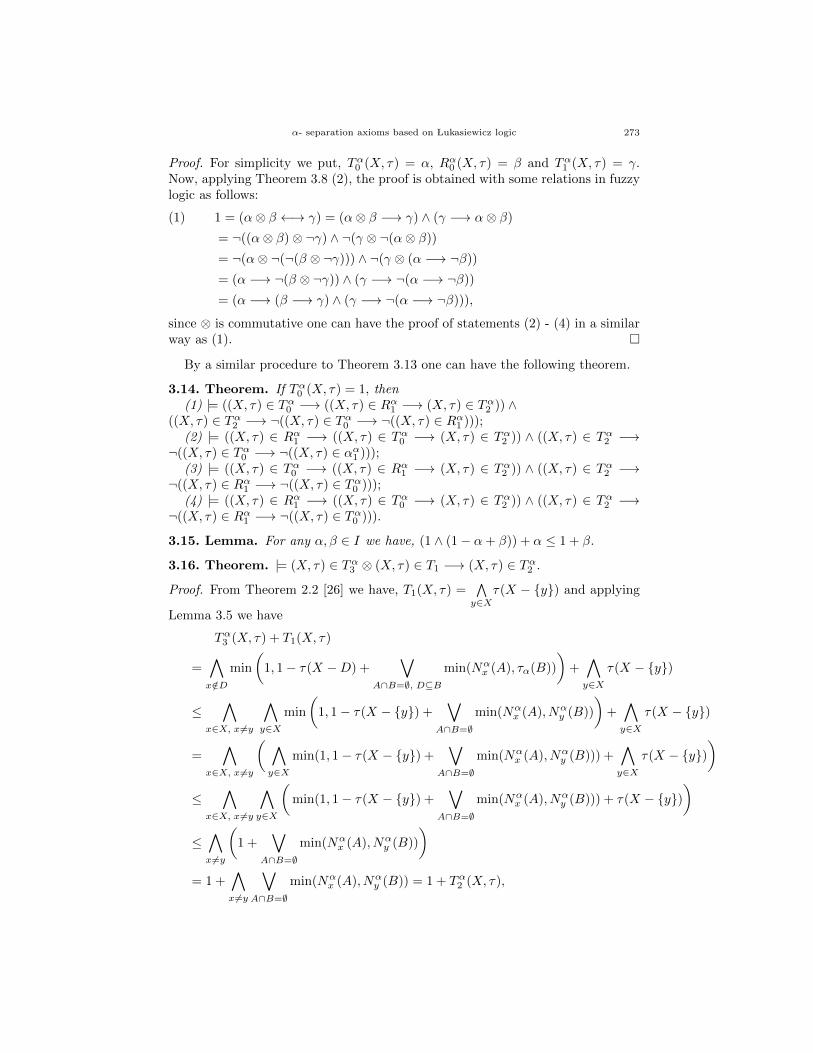
α- separation axioms based on Lukasiewicz logic
Proof. For simplicity we put, Tα0 (X, τ) = α, Rα0 (X, τ) = β and Tα1 (X, τ) = γ.Now, applying Theorem 3.8 (2), the proof is obtained with some relations in fuzzylogic as follows:
1 = (α⊗ β ←→ γ) = (α⊗ β −→ γ) ∧ (γ −→ α⊗ β)(1)
= ¬((α⊗ β)⊗ ¬γ) ∧ ¬(γ ⊗ ¬(α⊗ β))
= ¬(α⊗ ¬(¬(β ⊗ ¬γ))) ∧ ¬(γ ⊗ (α −→ ¬β))
= (α −→ ¬(β ⊗ ¬γ)) ∧ (γ −→ ¬(α −→ ¬β))
= (α −→ (β −→ γ) ∧ (γ −→ ¬(α −→ ¬β))),
since ⊗ is commutative one can have the proof of statements (2) - (4) in a similarway as (1).
By a similar procedure to Theorem 3.13 one can have the following theorem.
3.14. Theorem. If Tα0 (X, τ) = 1, then(1) |= ((X, τ) ∈ Tα0 −→ ((X, τ) ∈ Rα1 −→ (X, τ) ∈ Tα2 )) ∧
((X, τ) ∈ Tα2 −→ ¬((X, τ) ∈ Tα0 −→ ¬((X, τ) ∈ Rα1 )));(2) |= ((X, τ) ∈ Rα1 −→ ((X, τ) ∈ Tα0 −→ (X, τ) ∈ Tα2 )) ∧ ((X, τ) ∈ Tα2 −→
¬((X, τ) ∈ Tα0 −→ ¬((X, τ) ∈ αα1 )));(3) |= ((X, τ) ∈ Tα0 −→ ((X, τ) ∈ Rα1 −→ (X, τ) ∈ Tα2 )) ∧ ((X, τ) ∈ Tα2 −→
¬((X, τ) ∈ Rα1 −→ ¬((X, τ) ∈ Tα0 )));(4) |= ((X, τ) ∈ Rα1 −→ ((X, τ) ∈ Tα0 −→ (X, τ) ∈ Tα2 )) ∧ ((X, τ) ∈ Tα2 −→
¬((X, τ) ∈ Rα1 −→ ¬((X, τ) ∈ Tα0 ))).
3.15. Lemma. For any α, β ∈ I we have, (1 ∧ (1− α+ β)) + α ≤ 1 + β.
3.16. Theorem. |= (X, τ) ∈ Tα3 ⊗ (X, τ) ∈ T1 −→ (X, τ) ∈ Tα2 .Proof. From Theorem 2.2 [26] we have, T1(X, τ) =
∧y∈X
τ(X − y) and applying
Lemma 3.5 we have
Tα3 (X, τ) + T1(X, τ)
=∧
x/∈Dmin
(1, 1− τ(X −D) +
∨
A∩B=∅, D⊆Bmin(Nα
x (A), τα(B))
)+∧
y∈Xτ(X − y)
≤∧
x∈X, x 6=y
∧
y∈Xmin
(1, 1− τ(X − y) +
∨
A∩B=∅min(Nα
x (A), Nαy (B))
)+∧
y∈Xτ(X − y)
=∧
x∈X, x 6=y
( ∧
y∈Xmin(1, 1− τ(X − y) +
∨
A∩B=∅min(Nα
x (A), Nαy (B))) +
∧
y∈Xτ(X − y)
)
≤∧
x∈X, x 6=y
∧
y∈X
(min(1, 1− τ(X − y) +
∨
A∩B=∅min(Nα
x (A), Nαy (B))) + τ(X − y)
)
≤∧
x6=y
(1 +
∨
A∩B=∅min(Nα
x (A), Nαy (B))
)
= 1 +∧
x 6=y
∨
A∩B=∅min(Nα
x (A), Nαy (B)) = 1 + Tα2 (X, τ),
273
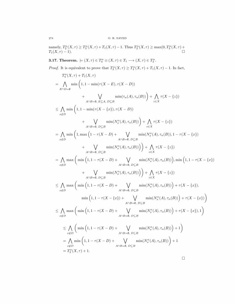
O. R. SAYED
namely, Tα2 (X, τ) ≥ Tα3 (X, τ) +T1(X, τ)− 1. Thus Tα2 (X, τ) ≥ max(0, Tα3 (X, τ) +T1(X, τ)− 1).
3.17. Theorem. |= (X, τ) ∈ Tα4 ⊗ (X, τ) ∈ T1 −→ (X, τ) ∈ Tα3 .
Proof. It is equivalent to prove that Tα3 (X, τ) ≥ Tα4 (X, τ) + T1(X, τ)− 1. In fact,
Tα4 (X, τ) + T1(X, τ)
=∧
E∩D=∅min
(1, 1−min(τ(X − E), τ(X −D))
+∨
A∩B=∅, E⊆A, D⊆Bmin(τα(A), τα(B))
)+∧
z∈Xτ(X − z)
≤∧
x/∈Dmin
(1, 1−min(τ(X − x), τ(X −D))
+∨
A∩B=∅, D⊆Bmin(Nα
x (A), τα(B))
)+∧
z∈Xτ(X − z)
=∧
x/∈Dmin
(1,max
(1− τ(X −D) +
∨
A∩B=∅, D⊆Bmin(Nα
x (A), τα(B)), 1− τ(X − x)
+∨
A∩B=∅, D⊆Bmin(Nα
x (A), τα(B))))
+∧
z∈Xτ(X − z)
=∧
x/∈Dmax
(min
(1, 1− τ(X −D) +
∨
A∩B=∅, D⊆Bmin(Nα
x (A), τα(B))),min
(1, 1− τ(X − x)
+∨
A∩B=∅, D⊆Bmin(Nα
x (A), τα(B))))
+∧
z∈Xτ(X − z)
≤∧
x/∈Dmax
(min
(1, 1− τ(X −D) +
∨
A∩B=∅, D⊆Bmin(Nα
x (A), τα(B)))
+ τ(X − x),
min(
1, 1− τ(X − x) +∨
A∩B=∅, D⊆Bmin(Nα
x (A), τα(B)))
+ τ(X − x))
≤∧
x/∈Dmax
(min
(1, 1− τ(X −D) +
∨
A∩B=∅, D⊆Bmin(Nα
x (A), τα(B)))
+ τ(X − x), 1)
≤∧
x/∈D
(min
(1, 1− τ(X −D) +
∨
A∩B=∅, D⊆Bmin(Nα
x (A), τα(B)))
+ 1
)
=∧
x/∈Dmin
(1, 1− τ(X −D) +
∨
A∩B=∅, D⊆Bmin(Nα
x (A), τα(B))
)+ 1
= Tα3 (X, τ) + 1.
274
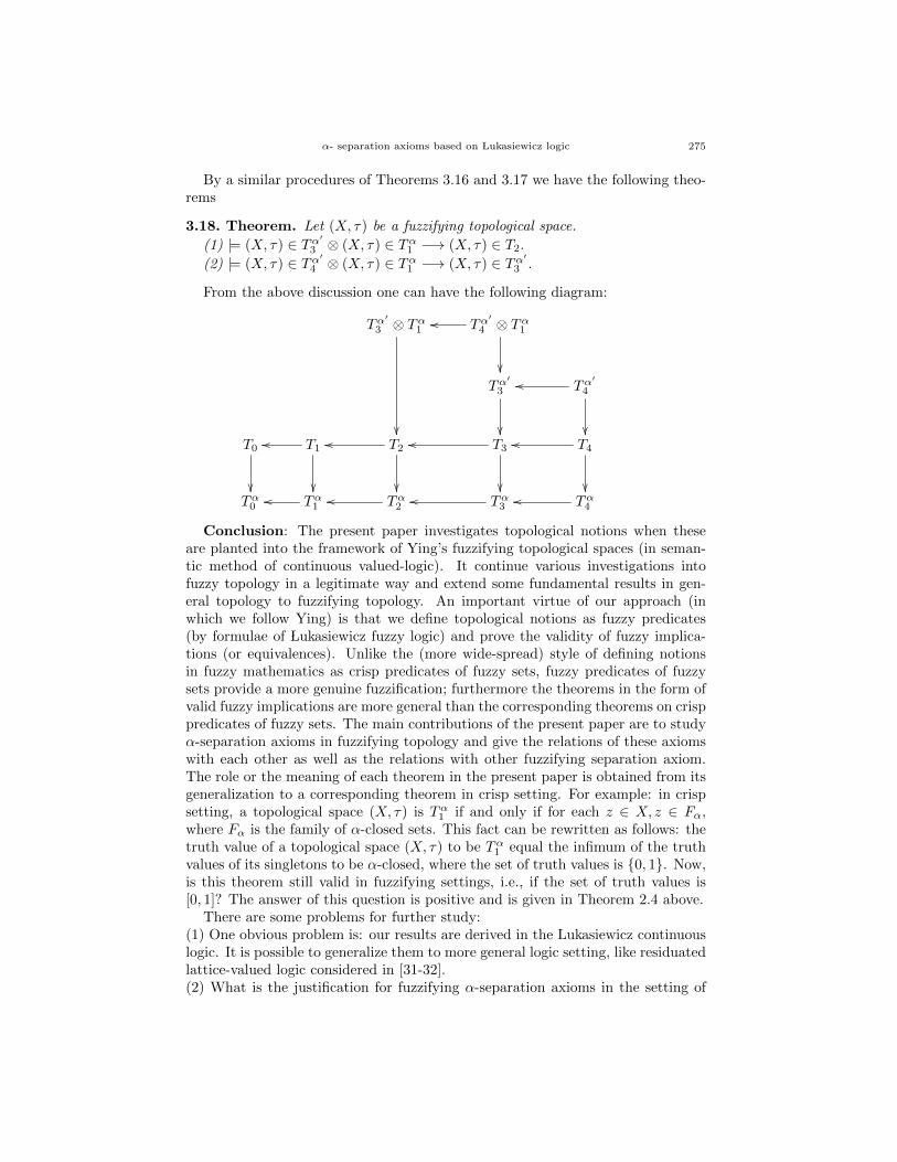
α- separation axioms based on Lukasiewicz logic
By a similar procedures of Theorems 3.16 and 3.17 we have the following theo-rems
3.18. Theorem. Let (X, τ) be a fuzzifying topological space.
(1) |= (X, τ) ∈ Tα′3 ⊗ (X, τ) ∈ Tα1 −→ (X, τ) ∈ T2.
(2) |= (X, τ) ∈ Tα′4 ⊗ (X, τ) ∈ Tα1 −→ (X, τ) ∈ Tα′3 .
From the above discussion one can have the following diagram:
Tα′
3 ⊗ Tα1
Tα′
4 ⊗ Tα1oo
Tα′
3
Tα′
4oo
T0
T1oo
T2oo
T3oo
T4oo
Tα0 Tα1oo Tα2oo Tα3oo Tα4oo
Conclusion: The present paper investigates topological notions when theseare planted into the framework of Ying’s fuzzifying topological spaces (in seman-tic method of continuous valued-logic). It continue various investigations intofuzzy topology in a legitimate way and extend some fundamental results in gen-eral topology to fuzzifying topology. An important virtue of our approach (inwhich we follow Ying) is that we define topological notions as fuzzy predicates(by formulae of Lukasiewicz fuzzy logic) and prove the validity of fuzzy implica-tions (or equivalences). Unlike the (more wide-spread) style of defining notionsin fuzzy mathematics as crisp predicates of fuzzy sets, fuzzy predicates of fuzzysets provide a more genuine fuzzification; furthermore the theorems in the form ofvalid fuzzy implications are more general than the corresponding theorems on crisppredicates of fuzzy sets. The main contributions of the present paper are to studyα-separation axioms in fuzzifying topology and give the relations of these axiomswith each other as well as the relations with other fuzzifying separation axiom.The role or the meaning of each theorem in the present paper is obtained from itsgeneralization to a corresponding theorem in crisp setting. For example: in crispsetting, a topological space (X, τ) is Tα1 if and only if for each z ∈ X, z ∈ Fα,where Fα is the family of α-closed sets. This fact can be rewritten as follows: thetruth value of a topological space (X, τ) to be Tα1 equal the infimum of the truthvalues of its singletons to be α-closed, where the set of truth values is 0, 1. Now,is this theorem still valid in fuzzifying settings, i.e., if the set of truth values is[0, 1]? The answer of this question is positive and is given in Theorem 2.4 above.
There are some problems for further study:(1) One obvious problem is: our results are derived in the Lukasiewicz continuouslogic. It is possible to generalize them to more general logic setting, like residuatedlattice-valued logic considered in [31-32].(2) What is the justification for fuzzifying α-separation axioms in the setting of
275

O. R. SAYED
(2, L) topologies.
(3) Obviously, fuzzifying topological spaces in [23] form a fuzzy category. Per-haps, this will become a motivation for further study of the fuzzy category.(4) What is the justification for fuzzifying α-separation axioms in (M,L)-topologiesetc.
References
[1] I. W. Alderton, α-compactness of fuzzy topological spaces: A categorical approach, Quas-
tiones Mathematicae, 20 (1997), 269-282.
[2] M. Caldas, D. N. Georgiou and S. Jafari, Characterizations of Low separation axioms viaα-open sets and α-closure operator, Bol. Soc. Paran. Mat., 21 (1-2)(2003), 1-14.
[3] M. Caldas, S. Jafari R. M. Latif and T. Noiri, Characterizations of functions with strongly
α-closed graphs, Scientific Studies and Research Series Mathematics and Informatics 19(1)(2009), 49-58.
[4] C. L. Chang, Fuzzy topological spaces, J. Math. Anal. Appl., 24 (1968), 182-190.
[5] J. A. Goguen, The fuzzy Tychonoff theorem, J. Math.Anal. Appl., 43 (1973), 182-190.[6] U. Hohle, Uppersemicontinuous fuzzy sets and applications, J. Math. Anal. Appl., 78 (1980),
659-673.[7] U. Hohle, Many Valued Topology and its Applications, Kluwer Academic Publishers, Dor-
drecht, 2001.
[8] U. Hohle, S. E. Rodabaugh, Mathematics of Fuzzy Sets: Logic, Topology, and MeasureTheory, in: Handbook of Fuzzy Sets Series, vol. 3, Kluwer Academic Publishers, Dordrecht,
1999.
[9] U. Hohle, S. E. Rodabaugh, A. Sostak, (Eds.), Special Issue on Fuzzy Topology, Fuzzy Setsand Systems, 73 (1995), 1-183.
[10] U. Hohle, A. Sostak, Axiomatic foundations of fixed-basis fuzzy topology, in: U. Hohle, S.E. Rodabaugh, (Eds.), Mathematics of Fuzzy Sets: Logic, Topology, and Measure Theory,
in: Handbook of Fuzzy Sets Series, vol. 3, Kluwer Academic Publishers, Dordrecht, 1999,
123-272.[11] J. L. Kelley, General Topology, Van Nostrand, New York, 1955.
[12] F. H. Khedr, F. M. Zeyada and O. R. Sayed, α-continuity and cα-continuity in fuzzifyingtopology, Fuzzy Sets and Systems, 116 (2000), 325-337.
[13] F.H. Khedr, F.M. Zeyada, O.R. Sayed, On separation axioms in fuzzifying topology Fuzzy
Sets and Systems 119 (2001), 439–458.[14] T. Kubiak, On Fuzzy Topologies, Ph.D. Thesis, Adam Mickiewicz University, Poznan,
Poland, 1985
[15] Y. M. Liu, M. K. Luo, Fuzzy Topology, World Scientific, Singapore, 1998.[16] S. N. Maheshwari and S. S. Thakur, On α-irresolute mappings, Tamkang J. Math., 11
(1980) 209-214.
[17] M. Maki, R. Devi and K. Balachandran,Generalized α-closed sets in topology, Bull. FukuokaUniv. Ed. Part III, 42 (1993) 13-21.
[18] A. N. Mahshour M. H. Ghanim and M. A. Fathalla, α-separation axioms and α-compactness
in fuzzy topological spaces, Rocky Mountain Journal of Mathematics, 16 (3)(1986) 591-600.
[19] T. Noiri, On α-continuous functions, Casopis Pest. Mat., 109 (1984) 118-126.
[20] D. Qiu, Characterizations of fuzzy finite automata, Fuzzy Sets and Systems, 141 (2004)391-414.
[21] D. Qiu, Fuzzifying topological linear spaces, Fuzzy Sets and Systems, 147 (2004) 249-272.
[22] I. L. Reilly and M. K. Vamanamurthy, On α-sets in topological spaces, Tamkang J. Math.,16 (1985) 7-11.
[23] S. E. Rodabaugh, Categorical foundations of variable-basis fuzzy topology, in: U. Hohle, S.
E. Rodabaugh, (Eds.), Mathematics of Fuzzy Sets: Logic, Topology, and Measure Theory,
276
α- separation axioms based on Lukasiewicz logic
in: Handbook of Fuzzy Sets Series, vol. 3, Kluwer Academic Publishers, Dordrecht, 1999,
273-388.
[24] S. E. Rodabaugh, The Hausdorff separation axioms for fuzzy topological spaces, TopologyAppl., 11 (1980) 319-334.
[25] J. B. Rosser, A. R. Turquette, Many-Valued Logics, North-Holland, Amsterdam, 1952.
[26] J. Shen, Separation axiom in fuzzifying topology, Fuzzy Sets and Systems 57 (1993), 111–123.
[27] G. J. Wang, Theory of L-Fuzzy Topological Spaces, Shanxi Normal University Press, Xi
an, 1988 (in Chinese).[28] M. S. Ying, A new approach for fuzzy topology (I), Fuzzy Sets and Systems, 39 (1991),
303-321.
[29] M. S. Ying, A new approach for fuzzy topology (II), Fuzzy Sets and Systems, 47 (1992),221-23.
[30] M. S. Ying, A new approach for fuzzy topology (III), Fuzzy Sets and Systems, 55 (1993),193-207.
[31] M. S. Ying, Fuzzifying topology based on complete residuated lattice-valued logic (I), Fuzzy
Sets and Systems, 56 (1993), 337-373.[32] M. S. Ying, Fuzzy Topology Based on Residuated Lattice-Valued Logic, Acta Mathematica
Sinica, 17 (2001), 89-102.
277

Hacettepe Journal of Mathematics and StatisticsVolume 43 (2) (2014), 279 – 281
Erratum and notes for near groups on nearnessapproximation spaces
Ebubekir Inan ∗† and Mehmet Ali Ozturk ‡
Keywords: Near set, Nearness approximation spaces, Near group.
2000 AMS Classification: 03E75, 03E99, 20A05, 20E99
Erratum and notes for: ”Inan, E., Ozturk, M. A. Near groups on nearnessapproximation spaces, Hacet J Math Stat, 41(4), 2012, 545–558.”
The authors would like to write some notes and correct errors in the originalpublication of the article [1]. The notes are given below:
0.1. Remark. In page 550, in Definition 3.1., (1) and (2) properties have to holdin Nr (B)
∗G. Sometimes they may be hold in ONr (B)
∗G, then G is not a near
group on nearness approximation space.
Example 3.3. and 3.4. are nice examples of this case. In Example 3.3., if weconsider associative property (b · e) · b = b · (e · b) for b, e ∈ H ⊂ G, we obtain ı = ı,but ı ∈ ONr (B)
∗H. Hence, we can observe that if the associative property
holds in ONr (B)∗H, then H can not be a subnear group of near group G.
Consequently, Example 3.3. and 3.4. are incorrect, i.e., they are not subneargroups of near group G.
0.2. Remark. Multiplying of finite number of elements in G may not alwaysbelongs to Nr (B)
∗G. Therefore always we can not say that xn ∈ Nr (B)
∗G, for
all x ∈ G and some positive integer n. If(Nr (B)
∗G, ·)
is groupoid, then we can
say that xn ∈ Nr (B)∗G, for all x ∈ R and all positive integer n.
In Example 3.2., the properties (1) and (2) hold in Nr (B)∗G. Hence G is a
near group on nearness approximation space.The corrections are given below:
In page 548, in subsection 2.4.1., definition of B-lower approximation of X ⊆ O
must be
B∗X =⋃
[x]B⊆X [x]B .
∗Department of Mathematics, Faculty of Arts and Sciences, Adıyaman University, Adıyaman,Turkey Email: [email protected]†Corresponding Author.‡Department of Mathematics, Faculty of Arts and Sciences, Adıyaman University, Adıyaman,
Turkey Email: [email protected]

In page 554, Theorem 3.8. must be as in Theorem 0.3:
0.3. Theorem. Let G be a near group on nearness approximation space, H anonempty subset of G and Nr (B)
∗H a groupoid. H ⊆ G is a subnear group of G
if and only if x−1 ∈ H for all x ∈ H.
Proof. Suppose that H is a subnear group of G. Then H is a near group andso x−1 ∈ H for all x ∈ H. Conversely, suppose x−1 ∈ H for all x ∈ H. By thehypothesis, since Nr (B)
∗H is a groupoid and H ⊆ G, then closure and associative
properties hold in Nr (B)∗H. Also we have x · x−1 = e ∈ Nr (B)
∗H. Hence H is
a subnear group of G.
In page 554, Theorem 3.9. must be as in Theorem 0.4:
0.4. Theorem. Let H1 and H2 be two near subgroups of the near group G andNr (B)
∗H1, Nr (B)
∗H2 groupoids. If
(Nr (B)∗H1) ∩ (Nr (B)
∗H2) = Nr (B)
∗(H1 ∩H2) ,
then H1 ∩H2 is a near subgroup of near group G.
Proof. Suppose H1 and H2 be two near subgroups of the near group G. Itis obvious that H1 ∩ H2 ⊂ G. Since Nr (B)
∗H1, Nr (B)
∗H2 are groupoids
and(Nr (B)
∗H1
)∩(Nr (B)
∗H2
)= Nr (B)
∗(H1 ∩H2), Nr (B)
∗(H1 ∩H2) is a
groupoid. Consider x ∈ H1 ∩H2. Since H1 and H2 are near subgroups, we havex−1 ∈ H1 and x−1 ∈ H2, i.e., x−1 ∈ H1 ∩H2. Thus from Theorem 0.3 H1 ∩H2 isa near subgroup of G.
In page 555, proof of Theorem 5.3. has some typos. It must be as in Theorem0.5:
0.5. Theorem. Let G be a near group on nearness approximation space and N asubnear group of G. N is a subnear normal group of G if and only if a ·n ·a−1 ∈ Nfor all a ∈ G and n ∈ N .
Proof. Suppose N is a near normal subgroup of near group G. We have a·N ·a−1 =N for all a ∈ G. For any n ∈ N , therefore we have a ·n · a−1 ∈ N . Suppose N is anear subgroup of near group G. Suppose a · n · a−1 ∈ N for all a ∈ G and n ∈ N .We have a ·N ·a−1 ⊂ N . Since a−1 ∈ G, we get a ·
(a−1 ·N · a
)·a−1 ⊂ a ·N ·a−1,
i.e., N ⊂ a · N · a−1. Since a · N · a−1 ⊂ N and N ⊂ a · N · a−1, we obtaina ·N · a−1 = N . Therefore N is a subnear normal group of G.
In page 556, Theorem 6.6. must be as in Theorem 0.6:
0.6. Theorem. Let G1 ⊂ O1,G2 ⊂ O2 be near groups that are near homomorphic,N near homomorphism kernel and Nr (B)
∗N a groupoid. Then N is a near normal
subgroup of G1.
In page 557, Theorem 6.7. must be as in Theorem 0.7:
0.7. Theorem. Let G1 ⊂ O1, G2 ⊂ O2 be near homomorphic groups, H1 and N1
a near subgroup and a near normal subgroup of G1, respectively and Nr1 (B)∗H1
groupoid. Then we have the following.
280

(1) If ϕ(Nr1 (B)
∗H1
)= Nr2 (B)
∗ϕ (H1), then ϕ (H1) is a near subgroup of
G2.
(2) if ϕ (G1) = G2 and ϕ(Nr1 (B)
∗N1
)= Nr2 (B)
∗ϕ (N1), then ϕ (N1) is a
near normal subgroup of G2.
In page 557, Theorem 6.8. must be as in Theorem 0.8:
0.8. Theorem. Let G1 ⊂ O1, G2 ⊂ O2 be near homomorphic groups, H2 and N2
a near subgroup and a near normal subgroup of G2, respectively and Nr1 (B)∗H1
groupoid. Then we have the following.
(1) if ϕ(Nr1 (B)
∗H1
)= Nr2 (B)
∗H2 , then H1 is a near subgroup of G1 where
H1 is the inverse image of H2.
(2) if ϕ (G1) = G2 and ϕ(Nr1 (B)
∗N1
)= Nr2 (B)
∗N2, then N1 is a near
normal subgroup of G1 where N1 is the inverse image of N2.
We apologize to the readers for any inconvenience of these errors might havecaused.
References
[1] Inan, E. and Ozturk, M. A. Near groups on nearness approximation spaces, Hacet J Math
Stat 41 (4), 545–558, 2012.
281


STATISTICS


Hacettepe Journal of Mathematics and StatisticsVolume 43 (2) (2014), 283 – 307
On estimating population parameters in thepresence of censored data: overview of available
methods
Abou El-Makarim A. Aboueissa∗
Abstract
This paper examines recent results presented on estimating populationparameters in the presence of censored data with a single detection limit(DL). The occurrence of censored data due to less than detectable mea-surements is a common problem with environmental data such as qual-ity and quantity monitoring applications of water, soil, and air samples.In this paper, we present an overview of possible statistical methods forhandling non-detectable values, including maximum likelihood, simplesubstitution, corrected biased maximum likelihood, and EM algorithmmethods. Simple substitution methods (e.g. substituting 0, DL/2, orDL for the non-detected values) are the most commonly used. It hasbeen shown via simulation that if population parameters are estimatedthrough simple substitution methods, this can cause significant biasin estimated parameters. Maximum likelihood estimators may pro-duce dependable estimates of population parameters even when 90% ofthe data values are censored and can be performed using a computerprogram written in the R Language. A new substitution method ofestimating population parameters from data contain values that arebelow a detection limit is presented and evaluated. Worked examplesare given illustrating the use of these estimators utilizing computerprogram. Copies of source codes are available upon request.
Keywords: detection limits, censored data, normal and lognormal distributions,likelihood function, maximum likelihood estimators.
1. Introduction
Environmental data frequently contain values that are below detection limits.Values that are below DL are reported as being less than some reported limitof detection, rather than as actual values. A data set for which all observationsmay be identified and counted, with some observations falling into the restrictedinterval of measurements and the remaining observations being fully measured,is said to be censored. A situation where observations may be censored would
∗Department of Mathematics and Statistics, University of Southern Maine, 96 Falmouth
Street, P.O. Box 9300, Portland, Maine 04104-9300, USA , Email: [email protected]

be chemical measurements where some observations have a concentration belowthe detection limit of the analytical method. A sample for which some observa-tions are known only to fall below a known detection limit, while the remainingobservations falling above the detection limit are fully measured and reported iscalled left-singly censored or simply left censored. Detection limits are usuallydetermined and justified in terms of the uncertainties that apply to a single rou-tine measurement. Left-censored data commonly arise in environmental contexts.Left-censored observations (observations reported as < DL) can occur when thesubstance or attribute being measured is either absent or exists at such low concen-trations that the substance is not present above the DL. In type I censoring, thedetection limit is fixed a priori for all observations and the number of the censoredobservations varies. In type II censoring, the number of censored observations isfixed a priori, and the detection limit vary.
The estimation of the parameters of normal and lognormal populations in thepresence of censored data has been studied by several authors in the context ofenvironmental data. There has been a corresponding increase in the amount ofattention devoted to the most proper analysis of data which have been collectedin related to environmental issues such as monitoring water and air quality, andmonitoring groundwater quality. The lognormal is frequently the parametric prob-ability distribution of choice used in fitting environmental data Gilbert (1987).However, Shumway et al. (1989) examined transformations to normality from
among the Box and Cox (1964) family of transformations: Y = Xλ−1λ for λ 6= 0,
and Y = ln(X) for λ = 0. The transformed variable Y is assumed to be normallydistributed with mean µ and standard deviation σ . Cohen (1959) used the methodof maximum likelihood to derive estimators for the µ and σ parameters from leftcensored samples. Cohen (1959) also provided tables that are needed to reportthese maximum likelihood estimates (MLEs). Aboueissa and Stoline (2004) in-troduced a new algorithm for computing Cohen (1959) MLE estimators of normalpopulation parameters from censored data with a single detection limit. Estima-tors obtained via this algorithm required no tables and more easily computed thanthe (MLEs) of Cohen (1959). Hass and Scheff (1990) compared methodologiesfor the estimation of the averages in truncated samples. Saw (1961) derived thefirst-order term in the bias of the Cohen (1959) MLE estimators for µ and σ,and proposed bias-corrected MLE estimators. Based on the bias-corrected tablesin Saw (1961b), Schneider (1984,1986) performed a least-squares fit to producecomputational formulas for normally distributed singly-censored data. Dempsteret. al. (1977) proposed an iterative method, called the expectation maximizationalgorithm (EM algorithm), for obtaining the maximum likelihood estimates forthese censored normal samples. The procedure consists of alternately estimatingthe censored observations from the current parameter estimates and estimatingthe parameters from the actual and estimated observations.
In practice, probably due to computational ease, simple substitution methodsare commonly used in many environmental applications. One of the most com-monly used replacement method is to substitute each left censored observation by
284

half of the detection limit DL, Helsel et al. (1986) and Helsel et al. (1988). Twosimple substitution methods were suggested by Gilliom and Helsel (1986). In onemethod, all left censored observations are replaced by zero. In the other method,all left censored observations are replaced by the detection limit DL. Aboueissaand Stoline (2004) developed closed form estimators for estimating normal popula-tion parameters from singly-left censored data based on a new replacement method.It has been shown that via simulation if left-censored observations are estimatedthrough these substitution methods, this can cause significant bias in estimatedparameters. In this article, a new substitution method, called weighted substi-tution method, is introduced and examined. This method is based on assigningdifferent weights for each left-censored observation. These weights are estimatedfrom the sample data prior to computing estimates of population parameters. Ithas been shown that via simulation if left-censored data are estimated through theweighted substitution method, this will reduce the bias in estimated parameters.Other suggested methods are discussed in Gibbons (1994), Gleit (1985), Schneider(1986), Gupta (1952), Stoline (1993), El-Shaarawi A. H. and Dolan D. M. (1989),El-Shaarawi and Esterby (1992), USEPA (1989), NCASI (1985, 1991), Gilliomand Helsel (1986), Helsel and Gilliom (1986), Helsel and Hirsch (1988), Schmee et.al. (1985), and Wolynetz (1979).
The objective of this article is to develop a new substitution method whichyield reliable estimates of population parameters from left-censored data, and alsoto compare the performances of the various estimation procedures. In addition,a simple-to-use computer program is introduced and described for estimating thepopulation parameters of normally or lognormally distributed left-censored datasets with a single detection limit using the eight parameter estimation methodsdescribed in this article. The authors of this article performed a simulation studyto asses the performance of various estimate procedures in terms of bias and meansquared error (MSE). Several methods, including MLE, bias-corrected MLE(UMLE), and EM algorithm (EMA), have been considered.
2. Methods Used for Estimation
To simplify the presentation in this section, the method is described and il-lustrated by reference to the analysis of normally distributed data, though thiscondition occurs infrequently in typical environmental data analysis. However,it is frequently necessary to transform real environmental data before analysis;typically the logarithmic transformation of xi = log(yi) is used, although othertransformations are possible. When the logarithmic or other transformation isused prior to censored data set analysis, it is necessary to transform the analysisresults back to the original scale of measurement following parameter estimation.
Let
mc−observations︷ ︸︸ ︷x1, ..., xmc︸ ︷︷ ︸left−censored
,
m−observations︷ ︸︸ ︷xmc+1, ..., xn︸ ︷︷ ︸non−censored
be a random sample of n observations of which
mc are left-censored while m = n−mc are non-censored (or fully measured) from
285

a normal population with mean µ and standard deviation σ . For censored obser-vations, it is only known that xj < DL for j = 1, ...,mc.
Let
(2.1) xm =1
m
n∑
i=mc+1
xi , and s2m =
1
m
n∑
i=mc+1
(xi − xm)2
be the sample mean and sample variance of the m non-censored observationsxmc+1, ..., xn.
2.1. MLE Estimators of Cohen. Cohen (1959) employed the method of max-imum likelihood to the normally distributed left-censored samples, and developedthe following MLE estimators for the mean and standard deviation in terms of atabulated function of two arguments:
(2.2) µ = xm − λ(xm −DL) ,
(2.3) σ =
√s2m + λ(xm −DL)2 ,
where
(2.4) λ = λ(h, γ), h =mc
nand γ =
s2m
(xm −DL)2
Cohen (1959) provided tables of the function λ = λ(γ, h) restricted to values ofγ = 0.00(0.05)1.00, and values of h = 0.01(0.01)0.10(0.05)0.70(0.10)0.90. The Co-hen (1959) method requires use of these tables. Schneider (1986) extended thesetables to include values of γ up to 1.48. Schmee et. al. (1985) extended thesetables further to include values of γ = 0.00(0.10)1.00(1.00)10.00 and values ofh = 0.10(0.10)0.90. However, interpolations for h and γ values are often requiredfor most applications.
2.2. Aboueissa and Stoline Algorithm for Computing MLE of Cohen.Aboueissa and Stoline (2004) introduced an algorithm for computing the CohenMLE estimators. This algorithm is based on solving the estimating equation
(2.5) γ =
(1− h
1−hφ(ξ)Φ(ξ) ( h
1−hφ(ξ)Φ(ξ) − ξ)
)
( h1−h
φ(ξ)Φ(ξ) − ξ)2
,
numerically for ξ (say ξ). With ξ obtained via this algorithm, the exact value ofthe λ-parameter is then given by:
(2.6) λas = λ(h, ξ) =Y (h, ξ)
Y (h, ξ)− ξ,
where
Y = Y (h, ξ) =
(h
1− h
)Z(ξ),
286

Z(ξ) =φ(−ξ)
1− Φ(−ξ) , and h =mc
n= CL = censoring level .
The functions φ(ξ) and Φ(ξ) are the pdf and cdf of the standard unit normal.
with λas obtained from (2.6), the MLE estimators obtained via this algorithmare obtained from (2.2) and (2.3) as:
(2.7) µas = xm − λas(xm −DL) ,
and
(2.8) σas =
√s2m + λas(xm −DL)2 .
MLE estimators obtained via this method are labeled the ASAMLEOC methodin this article. It should be noted that the ASAMLEOC method can be used toobtain the MLE estimators of population parameters from censored samples forall values of h and γ without any restrictions, and for all censoring levels includ-ing censoring levels greater than 0.90. The ASAMLEOC estimators µas and σasgiven by (2.7) and (2.8) are essentially Cohen’s (1959) MLE estimators, which areobtained without the use of any auxiliary tables. It should also be noted that Co-hen’s (1959) method can not be used to obtain the maximum likelihood estimatesfrom censored samples that have a censoring level higher than 90% (h > 0.90).
2.3. Bias-Corrected MLE Estimators. Saw (1961) derived the first-orderterm in the bias of the MLE estimators of µ and σ and proposed bias-correctedMLE estimators. Based on the bias-corrected tables in Saw (1961), Schneider(1986) performed a least-squares fit to produce computational formulas for theunbiased MLE estimators of µ and σ from normally distributed singly-censoreddata. These formulas, for the singly left-censored samples can be written as
(2.9) µu = µ− σBun+ 1
, and σu = σ − σBσn+ 1
,
where µ and σ are the MLE estimators of Cohen (1959) or equivalently theASAMLE estimators µas and σas, and
(2.10) Bu = −e2.692− 5.439mn+1 and Bσ = −
(0.312 +
0.859m
n+ 1
)−2
.
This method will be referred to as the UMLE method in this paper.
2.4. Haas and Scheff Estimators(1990). Haas and Scheff (1990)developed apower series expansion that fits the tabled values of the auxiliary function λ(γ, h)to within 6% for Cohen’s (1959) estimates. This power series expansion is givenby:
(2.11)
287
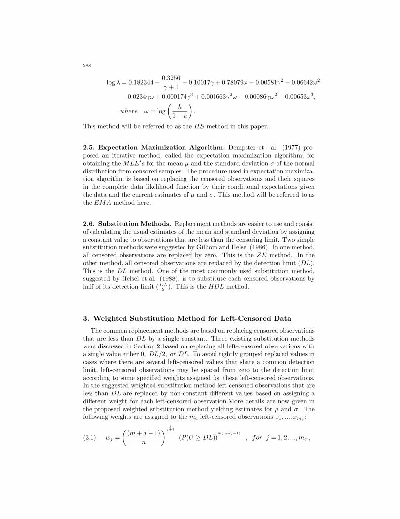
log λ = 0.182344− 0.3256
γ + 1+ 0.10017γ + 0.78079ω − 0.00581γ2 − 0.06642ω2
− 0.0234γω + 0.000174γ3 + 0.001663γ2ω − 0.00086γω2 − 0.00653ω3,
where ω = log
(h
1− h
).
This method will be referred to as the HS method in this paper.
2.5. Expectation Maximization Algorithm. Dempster et. al. (1977) pro-posed an iterative method, called the expectation maximization algorithm, forobtaining the MLE′s for the mean µ and the standard deviation σ of the normaldistribution from censored samples. The procedure used in expectation maximiza-tion algorithm is based on replacing the censored observations and their squaresin the complete data likelihood function by their conditional expectations giventhe data and the current estimates of µ and σ. This method will be referred to asthe EMA method here.
2.6. Substitution Methods. Replacement methods are easier to use and consistof calculating the usual estimates of the mean and standard deviation by assigninga constant value to observations that are less than the censoring limit. Two simplesubstitution methods were suggested by Gilliom and Helsel (1986). In one method,all censored observations are replaced by zero. This is the ZE method. In theother method, all censored observations are replaced by the detection limit (DL).This is the DL method. One of the most commonly used substitution method,suggested by Helsel et.al. (1988), is to substitute each censored observations byhalf of its detection limit (DL2 ). This is the HDL method.
3. Weighted Substitution Method for Left-Censored Data
The common replacement methods are based on replacing censored observationsthat are less than DL by a single constant. Three existing substitution methodswere discussed in Section 2 based on replacing all left-censored observations witha single value either 0, DL/2, or DL. To avoid tightly grouped replaced values incases where there are several left-censored values that share a common detectionlimit, left-censored observations may be spaced from zero to the detection limitaccording to some specified weights assigned for these left-censored observations.In the suggested weighted substitution method left-censored observations that areless than DL are replaced by non-constant different values based on assigning adifferent weight for each left-censored observation.More details are now given inthe proposed weighted substitution method yielding estimates for µ and σ. Thefollowing weights are assigned to the mc left-censored observations x1, ..., xmc :
(3.1) wj =
((m+ j − 1)
n
) jj+1
(P (U ≥ DL))ln(m+j−1)
, for j = 1, 2, ...,mc ,
288

where the probability P (U ≥ DL) is estimated from the sample data by:
(3.2) P (U ≥ DL) = 1− Φ
(DL− xm
sm
)
An extensive simulation study was conducted on several weights. The simulationresults (shown in the appendix) indicate that the proposed estimators using (3.1)are superior to those using the other weights in the sense of mean square error(variance of the estimator plus the square of the bias) in addition to the abilityto recover the true mean and standard deviation as well as the existing methodssuch as maximum likelihood and EM algorithm estimators.
Estimates of the weights given in (3.1) are given by:
(3.3) wj =
((m+ j − 1)
n
) jj+1 (
P (U ≥ DL))ln(m+j−1)
.
where the distribution of U is approximated by a normal distribution with an es-timated mean xm and an estimated variance s2
m.
These weights are selected on a trial and error basis by means of simulationsto yield estimators of population parameters that perform nearly as well as es-timators obtained via the existing methods such as MLE estimators and EMAmethod. Left-censored observations x1, x2, ..., xmc are then replaced by the follow-ing weighted mc observations:
(3.4) (xw1 , xw2 , ..., x
wmc) ≡ (w1DL, w2DL, ..., wmcDL)
Let
(3.5) xmc =1
mc
mc∑
i=1
xwi , and s2mc =
1
mc
mc∑
i=1
(xwi − xmc)2
be the sample mean and sample variance of the weightedmc observations xw1 , xw2 , ..., x
wmc .
The corresponding weighted substitution method estimators µw and σw of µ andσ are given by, respectively:
(3.6)µw =
1
n
(mc∑
i=1
xwi +n∑
i=mc+1
xi
)
= xm − λµw (xm − xmc) ,and
(3.7)
σw =
√√√√ 1
n
(mc∑
i=1
(xwi − µw)2 +n∑
i=mc+1
(xi − µw)2
)
=
√m s2
m +mc s2mc
n+ λσw (xm − xmc)2 ,
289

where
(3.8) λµw =mc
nand λσw =
m mc
n2.
It should be noted that µw in (3.6) can be written as:
(3.9) µw =m xm +mc xmc
n,
which is the weighted average of the sample means xm and xmc of fully measuredand weighted observations, respectively. It should also be observed that σw in(3.7) can be written as:
(3.10) σw =
√s2w + λσw (xm − xmc)2
where s2w =
m s2m+mc s2mc
n is the weighted average of the sample variances s2m and
s2mc of fully measured and weighted observations, respectively. Extensive simula-
tion results show that use of the WSM method leads to estimators that have theability to recover the true population parameters as well as the maximum likeli-hood estimators, and are generally superior to the constant replacement methods.In environmental sciences such as applied medical and environmental studies mostof the data sets include non-detected (or left-censored) data values. The use ofstatistical methods such as the proposed one allows estimates of population pa-rameters from data under consideration.
Asymptotic Variances of Estimates: The asymptotic variance-covariance ma-trix of the maximum likelihood estimates (µ, σ) is obtained by inverting theFisher information matrix I with elements that are negatives of expected val-ues of the second-order partial derivatives of the log-likelihood function with re-spect to the parameters evaluated at the estimates µ and σ. The asymptoticvariance-covariance matrix showed by Cohen (1991, 1959), will be used to obtainthe estimated asymptotic variances of both µ and σ. Cohen (1959) describes theestimated asymptotic variance-covariance matrix of (µ, σ) by
Cov(µ, σ) =
( σ2
n[1−Φ(ξ)]) ϕ22
ϕ11ϕ22−ϕ212
( σ2
n[1−Φ(ξ)]) −ϕ12
ϕ11ϕ22−ϕ212
( σ2
n[1−Φ(ξ)]) −ϕ12
ϕ11ϕ22−ϕ212
( σ2
n[1−Φ(ξ)]) ϕ11
ϕ11ϕ22−ϕ212
where
ϕ11 = ϕ11(ξ) = 1 + Z(ξ)[Z(−ξ) + ξ]
ϕ12 = ϕ12(ξ) = Z(ξ)(
1 + ξ[Z(−ξ) + ξ])
ϕ22 = ϕ22(ξ) = 2 + ξϕ12
For the ASAMLEOC ξ is the solution of (2.5) as described in the previous sec-
tion. For all other methods, without loss of generality, ξ = DL−µσ .
290

4. Computer Programs
To facilitate the application of parameter estimation methods described in thisarticle, a computer programs is presented to automate parameters estimation fromleft-censored data sets that are normally or lognormally distributed. This com-puter program is called ”SingleLeft.Censored.Normal.Lognormal.estimates”,and is written in the R language. The EM Algorithm method has been pro-grammed in the R language. The program is called ”EMA.Method”, and is pre-sented as a part of the main computer program ”SingleLeft.Censored.Normal.Lognormal.estimates”.Copies of source codes are available upon request.
5. Worked Example
The guidance document Statistical Analysis of Ground-Water Monitoring Dataat RCRA Facilities, Interim Final Guidance (USEPA, 1989b) contains an ex-ample involving a set of sulfate concentrations (mg/L) in which three values arereported as (< 1450 = DL). The sulfate concentrations are assumed to come froma normal distribution. These 24 sulfate concentration values are:
< 1, 450 1, 800 1, 840 1, 820 1, 860 1, 780 1, 760 1, 8001, 900 1, 770 1, 790 1, 780 1, 850 1, 760 < 1, 450 1, 7101, 575 1, 475 1, 780 1, 790 1, 780 < 1, 450 1, 790 1, 800
For this sample n = 24, m = 21, mc = 3, h = 324 . The sample mean and the sample
variance of the non-censored sample values are xm = 1771.905 and s2m = 8184.467.
WSM Method: From (3.3) and (3.4) we obtain the estimate weights and theweighted data as follows:
(w1 , w2 , w3) = (0.9348828 , 0.9430983 , 0.9680175),
and
(xw1 , xw2 , xw3 ) = (1355.580 , 1367.493 , 1403.625).
The updated data set (fully measured and weighted data) is given by:
1,355.580 1, 800 1, 840 1, 820 1, 860 1, 780 1, 760 1, 8001, 900 1, 770 1, 790 1, 780 1, 850 1, 760 1,367.493 1, 7101, 575 1, 475 1, 780 1, 790 1, 780 1,403.625 1, 790 1, 800
The sample mean xmc and sample variance s2mc of the weighted data xw1 , xw2 , xw3
are given by:
xmc = 1375.566 and s2mc = 417.3153
From (3.8) we obtain
λµw =mc
n=
3
24= 0.125 and λσw =
m mc
n=
(21)(3)
242= 0.109375 .
Accordingly, using estimators (3.6) - (3.7) we calculate the WSM method estima-tors µw and σw as:
µw = 1771.905− 0.125(1771.905− 1375.566) = 1722.3626 ,
291
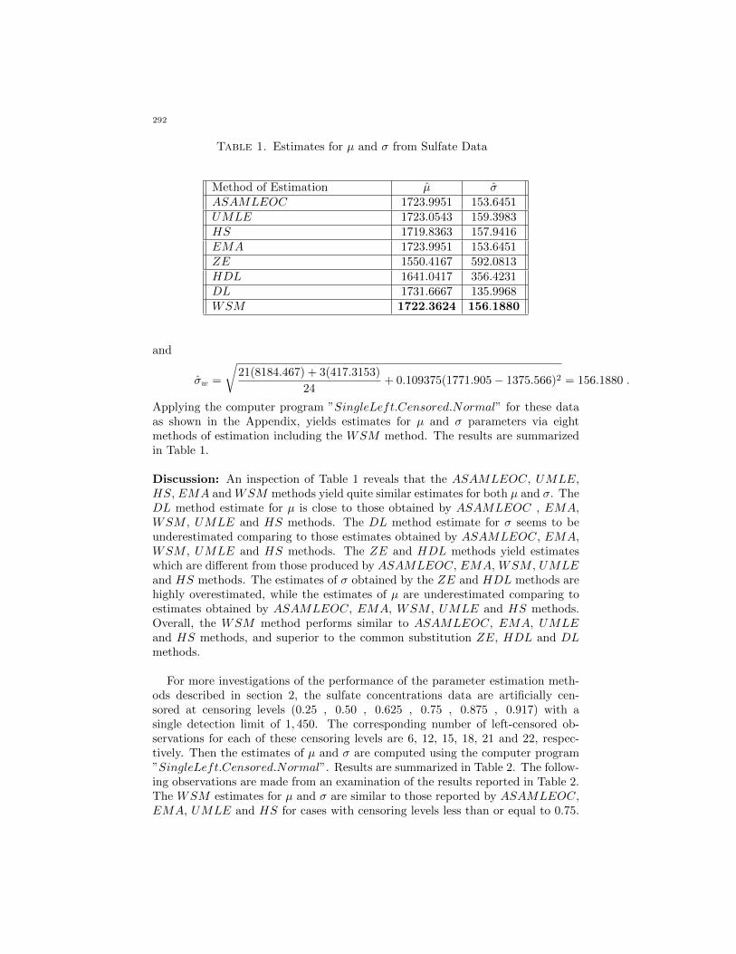
Table 1. Estimates for µ and σ from Sulfate Data
Method of Estimation µ σASAMLEOC 1723.9951 153.6451UMLE 1723.0543 159.3983HS 1719.8363 157.9416EMA 1723.9951 153.6451ZE 1550.4167 592.0813HDL 1641.0417 356.4231DL 1731.6667 135.9968WSM 1722.3624 156.1880
and
σw =
√21(8184.467) + 3(417.3153)
24+ 0.109375(1771.905− 1375.566)2 = 156.1880 .
Applying the computer program ”SingleLeft.Censored.Normal” for these dataas shown in the Appendix, yields estimates for µ and σ parameters via eightmethods of estimation including the WSM method. The results are summarizedin Table 1.
Discussion: An inspection of Table 1 reveals that the ASAMLEOC, UMLE,HS, EMA and WSM methods yield quite similar estimates for both µ and σ. TheDL method estimate for µ is close to those obtained by ASAMLEOC , EMA,WSM , UMLE and HS methods. The DL method estimate for σ seems to beunderestimated comparing to those estimates obtained by ASAMLEOC, EMA,WSM , UMLE and HS methods. The ZE and HDL methods yield estimateswhich are different from those produced by ASAMLEOC, EMA, WSM , UMLEand HS methods. The estimates of σ obtained by the ZE and HDL methods arehighly overestimated, while the estimates of µ are underestimated comparing toestimates obtained by ASAMLEOC, EMA, WSM , UMLE and HS methods.Overall, the WSM method performs similar to ASAMLEOC, EMA, UMLEand HS methods, and superior to the common substitution ZE, HDL and DLmethods.
For more investigations of the performance of the parameter estimation meth-ods described in section 2, the sulfate concentrations data are artificially cen-sored at censoring levels (0.25 , 0.50 , 0.625 , 0.75 , 0.875 , 0.917) with asingle detection limit of 1, 450. The corresponding number of left-censored ob-servations for each of these censoring levels are 6, 12, 15, 18, 21 and 22, respec-tively. Then the estimates of µ and σ are computed using the computer program”SingleLeft.Censored.Normal”. Results are summarized in Table 2. The follow-ing observations are made from an examination of the results reported in Table 2.The WSM estimates for µ and σ are similar to those reported by ASAMLEOC,EMA, UMLE and HS for cases with censoring levels less than or equal to 0.75.
292

Table 2. Estimates for µ and σ from Sulfate Data with artificial
censoring levels
mc = 6, CL = 0.25 mc = 12, CL = 0.50 mc = 15, CL = 0.625
Method of Estimation µ σ µ σ µ σ
ASAMLEOC 1658.6581 205.1465 1497.0883 313.4529 1367.1360 361.7728
UMLE 1656.2454 214.6244 1483.4885 337.3514 1336.9885 399.2681
HS 1651.2191 210.7608 1484.2813 320.0817 1351.8316 368.3523
EMA 1658.6581 205.1465 1497.1077 313.4304 1367.8667 361.0457
ZE 1322.9166 768.2189 888.9583 890.6903 661.4583 855.3307
HDL 1504.1667 457.3376 1251.4583 529.3775 1114.5833 505.3091
DL 1685.4167 158.9478 1613.9583 173.1027 1567.7083 159.5957
WSM 1647.8992 218.9194 1456.3776 341.5274 1314.6978 382.7615
mc = 18, CL = 0.75 mc = 21, CL = 0.875 mc = 22, CL = 0.917
ASAMLEOC 1191.5900 412.5770 815.9108 564.2837 623.1800 605.8733
UMLE 1125.5549 474.0433 642.4414 695.2905 391.6580 773.0710
HS 1170.5134 420.0236 801.0685 568.6071 633.4851 603.1457
EMA 1204.8421 401.5795 996.7565 443.5979 996.0501 381.4442
ZE 436.0417 756.5147 222.5000 588.7080 147.5000 489.2107
HDL 979.7917 443.4793 856.875 348.9562 812.0833 288.8372
DL 1523.5417 134.6947 1491.2500 109.2898 1476.6667 88.4904
WSM 1149.1283 406.4031 968.9359 419.4892 897.6092 410.0749
For cases with censoring levels above 0.75, the WSM and EMA methods yieldsimilar results. For cases with censoring levels less than 0.75, µ is underestimatedby both ZE and HDL Methods, while σ is overestimated comparing to estimatesobtained by ASAMLEOC, EMA, UMLE and HS methods. The DL methodyield similar estimate for µ for cases with censoring levels less than 0.75, while σ isunderestimated for all censoring levels via this method comparing to estimates ob-tained by ASAMLEOC of Cohen, EMA, UMLE and HS methods. Overall, theWSM method yields similar estimates to those obtained by ASAMLEOC, EMA,UMLE and HS methods, and superior to the existing substitution methods ZE,HDL and DL for all censoring levels.
6. Comparison of Methods
In this section the estimation methods described above were compared by a sim-ulation study. We shall assess the performance of estimators obtained via thesemethods in terms of the mean squared error MSE (variance of the estimator plusthe square of the bias). The simulation study was performed with ten thousandrepetitions (N = 10000) of samples from a normal distribution for each combina-tion of n, µ, σ, and the censoring level CL = h. Simulations were conducted withcensoring levels 0.15, 0.25, 0.50, 0.75, and 0.90. The selected combinations of(n, µ, σ, CL) are:
(6.1)
n = 10, 25, 50, 75, 100 , µ = 25 , σ = 10, CL = 0.15n = 10, 25, 50, 75, 100 , µ = 25 , σ = 10, CL = 0.25n = 10, 25, 50, 75, 100 , µ = 25 , σ = 10, CL = 0.50n = 10, 25, 50, 75, 100 , µ = 10 , σ = 5, CL = 0.75n = 10, 25, 50, 75, 100 , µ = 10 , σ = 5, CL = 0.90
Given the censoring level CL, the detection limit is computed from the relationDL = CLth percentile. The data sets were then artificially censored at DL. Any
293

value falling below DL was considered to be left-censored. These simulated datasets (N = 10000 for each combination of n, µ, σ and CL) were then utilized bythese estimators to obtain estimates of µ and σ. The average of the N = 10000estimates are reported as µ and σ in Table 1 and 2. The MSE based on N = 10000simulation runs are also reported in each table. The MSE of µ is defined by:
(6.2) MSE(µ, µ) = V ar(µ) + (b(µ, µ))2,
where
(6.3) b(µ, µ) = µ− µ ,is the bias of µ, where
(6.4) µ =1
N
N∑
i=1
µi and V ar(µ) =1
N − 1
N∑
i=1
(µi − µ)2.
The MSE of σ can be defined in a similar way.
Estimation Methods: The methods used for the estimation of the normal pop-ulation parameters from singly-left-censored samples are:
ASAMLEOC: Aboueissa and Stoline Algorithm for Calculating MLE of Cohen,UMLE: Bias-Corrected MLE Estimators,
HS: Haas and Scheff method,EMA: Expectation Maximization algorithm method,ZE: Replacing all left-censored data by zero method,
HDL: Replacing all left-censored data by half of the detection limit method,DL: Replacing all left-censored data by the detection limit method,
WSM : The new Weighted Substitution Method.
Tables 4 and 5 are partitioned into 5 subgroups by increasing censoring level:CL = 0.15, 0.25, 0.50, 0.75 and 0.90. The simulation results within each subgroupare further partitioned by increasing sample size n = 10, 25, 50 and 75. Twosimulation results are given for each method and for each combination of n, µ, σand CL. These are the average value of the estimate and the MSE.
6.1. Comparison of Methods: µ Parameter.WSM to existing methods: The following observations and conclusions aremade from an examination of the simulation results reported for the mean µ.
For the µ = 25 parameter value: the reported new WSM method estimatesare all in the range 24.8722 − 25.2874, the reported HDL method estimates areall in the range 23.7069 − 24.6108, the reported EMA method estimates are allin the range 24.7206 − 25.002 and the reported ASAMLEOC method estimatesare all in the range 24.5856− 25.0355 for cases with censoring level less than 50%.For cases with censoring levels less than 50%: (1) the MSE values for HDLmethod are larger than those reported by the new WSM method, and (2) theMSE values for WSM method are nearly equal to those reported by the newEMA and ASAMLEOC methods. For cases with censoring level 50%: the re-ported new WSM method estimates are all in the range 23.4630 − 24.6600, thereported HDL method estimates are all in the range 22.5559 − 22.9255, the re-ported EMA method estimates are all in the range 24.8221 − 25.0050 and the
294
reported ASAMLEOC method estimates are all in the range 25.0019− 25.4548.The MSE values for HDL method are larger than those reported by the newWSM method. The MSE values for the new WSM method are nearly equal tothose reported by both EMA and ASAMLEOC methods except for cases withsample sizes 50, 75, and 100.
For the µ = 10 parameter value and for cases with censoring level greaterthan or equal to 75%: the reported new WSM method estimates are all inthe range 8.5887 − 9.8231, the reported HDL method estimates are all in therange 8.6633 − 9.2154, the reported EMA method estimates are all in the range10.1079−12.7350 and the reported ASAMLEOC method estimates are all in therange 9.8679− 11.2427. The MSE values for HDL and EMA methods are quitesimilar and smaller than those reported by EMA and ASAMLEOC methods ex-cept for cases with sample sizes 75 and 100. For cases with censoring level 90%and sample size 10, it has been noted that estimates for the µ parameter are notavailable via EMA method.
Overall, the new WSM method appears to be superior to the existing meth-ods for cases with censoring levels less than 50%, and superior to EMA andASAMLEOC methods for cases with censoring levels greater than or equal to50% except for cases with sample sizes 75 and 100. The new WSM and HDLmethods yield quite similar estimates for the µ parameter for cases with censoringlevels greater than or equal to 50%.
6.2. Comparison of Methods: σ Parameter.WSM to existing methods: The following observations and conclusions aremade from an examination of the simulation results reported for the standard de-viation σ.
For the σ = 10 parameter value: the reported new WSM method estimates areall in the range 9.2886 − 9.8007, the reported HDL method estimates are all inthe range 10.2680 − 10.7815, the reported EMA method estimates are all in therange 9.6781− 10.0459 and the reported ASAMLEOC method estimates are allin the range 9.5468 − 10.0068 for cases with censoring level less than 50%. TheMSE values for EMA and ASAMLEOC methods are larger than those reportedby the new WSM method for cases with censoring levels less than 50%. TheMSE values reported by HDL and the new WSM methods are quite similar forcases with censoring levels less than 50%. For cases with censoring level 50%:the reported new WSM method estimates are all in the range 9.3601 − 10.5496,the reported HDL method estimates are all in the range 10.7585 − 11.0397, thereported EMA method estimates are all in the range 9.5578− 9.9383 and the re-ported ASAMLEOC method estimates are all in the range 9.1672− 9.8955. TheMSE values for HDL and the new WSM methods are quite similar, and smallerthan those reported by both EMA and ASAMLEOC methods except for caseswith sample sizes 100.
295

For the σ = 5 parameter value and for cases with censoring level greaterthan or equal to 75%: the reported new WSM method estimates are all inthe range 4.3496 − 5.0428, the reported HDL method estimates are all in therange 3.0071 − 4.3463, the reported EMA method estimates are all in the range3.0289 − 4.8167 and the reported ASAMLEOC method estimates are all in therange 3.8187 − 4.9756. The MSE values for EMA, EMA and ASAMLEOCmethods are larger than those reported by the new WSM method. For cases withcensoring level 90% and sample size 10, it has been noted that estimates for the σparameter are not available via EMA method. It should be noted that the σ = 5parameter value for most cases is highly under estimated by EMA, EMA andASAMLEOC methods.
Overall, the new WSM method appears to be superior to HDL method forcases with censoring levels greater than or equal to 50%, and superior to EMAand ASAMLEOC methods for all censoring cases. The HDL and the new WSMmethods perform similarly for cases with censoring levels less than 50%.
In summary, the maximum likelihood estimators (ASAMLEOC), the new weightedsubstitution method estimators (WSM), and the EM algorithm estimators (EMA)perform similarly, and all are generally superior to the existing substitution methodestimators.
6.3. Additional Simulation Results.The following simulation results are obtained using the following combinations ofn, µ, σ, and censoring level CL.
Table 3. Estimates for µ and σ from Sulfate Data
(n, µ, σ) k CL(k, 25, 10) k = 10, 25, 50, 75, 100 0.75 - 0.90(k, 10, 5) k = 10, 25, 50, 75, 100 0.15 - 0.50(k, 20, 3) k = 10, 25, 50, 75, 100 0.10 - 0.90
Tables 6, 7 and 8 are partitioned into two subgroups. Each subgroup has a differ-ent censoring level. The simulation results within each subgroup are given for bothpopulation mean µ and standard deviation σ. Two simulation results are givenfor each method and for each combination of n, µ, σ and CL. These simulationresults are the average value of the estimate and the MSE.
296

Table 4. Simulation Estimates of the Mean µ from Normally Dis-
tributed Left-Censored Samples with a Single Detection Limit
Methods Of Estimation
MLE Replacement(n, µ, σ) EMA ASAMLEOC UMLE HS WSM ZE HDL DL
CL = 0.15
(10, 25, 10) µMSE
24.720612.9903
24.585612.1390
24.336712.4803
24.416012.3479
25.030310.2139
22.449714.1331
24.051710.3785
25.653612.1721
(25, 25, 10) µMSE
25.00224.0587
25.00474.0515
24.93024.0600
24.87024.0765
25.28743.6776
23.38205.5471
24.60563.5844
25.82924.7208
(50, 25, 10) µMSE
24.98731.9815
24.96101.9524
24.92211.9576
24.82291.9836
25.21751.7494
23.40543.9807
24.60451.8237
25.80362.5930
(75, 25, 10) µMSE
24.95691.3018
24.91671.2937
24.88921.2997
24.77571.3415
25.15201.2036
23.37723.5491
24.56541.2649
25.75361.8417
(100, 25, 10) µMSE
24.93031.0832
24.94551.0840
24.93081.0861
24.81731.1177
25.11871.0118
23.50413.0278
24.61081.0706
25.71761.5900
CL = 0.25
(10, 25, 10) µMSE
24.931411.1167
24.770510.1121
24.360610.6242
24.556410.2893
25.13878.6504
20.814722.7221
23.70698.7693
26.599112.2048
(25, 25, 10) µMSE
24.85674.7220
25.03554.4562
24.92784.4708
24.88424.4865
25.06513.8785
21.942611.9771
24.17284.0882
26.40316.3499
(50, 25, 10) µMSE
24.93792.3519
24.90312.2546
24.84052.2750
24.71762.3375
24.98841.9278
21.690612.1852
24.07832.4918
26.46594.3222
(75, 25, 10) µMSE
24.91991.3578
24.91751.3316
24.87981.3406
24.74031.3983
24.87451.1832
21.792311.0518
24.10971.7847
26.42723.3294
(100, 25, 10) µMSE
24.97921.0849
25.00241.0738
24.97701.0749
24.82921.1061
24.87220.9745
21.901610.2353
24.19361.4676
26.48573.2606
CL = 0.50
(10, 25, 10) µMSE
24.822118.5532
25.186815.2003
24.150617.3134
24.909115.4780
24.660010.1436
16.284879.3801
22.555912.9385
28.827027.0316
(25, 25, 10) µMSE
24.97786.7314
25.45486.3569
25.09366.3417
25.20666.3287
23.88735.2874
16.903267.0511
22.92557.2413
28.947920.7299
(50, 25, 10) µMSE
24.93823.2269
25.00192.9649
24.80383.0511
24.70913.1225
23.87584.0171
16.434174.0480
22.68246.7341
28.930717.8859
(75, 25, 10) µMSE
25.00501.9961
25.15571.9971
25.02371.9946
24.87492.0344
23.760424.2894
16.627870.5353
22.80105.7310
28.974217.3938
(100, 25, 10) µMSE
24.94961.4499
24.99601.3884
24.89801.4097
24.70151.5089
23.46305.1825
16.447173.4808
22.69535.9611
28.943416.6976
CL = 0.75
(10, 10, 5) µMSE
11.16004.9783
10.92946.9497
9.76948.5266
10.71346.9843
9.82312.3121
4.607929.4568
9.13312.5634
13.658216.9481
(25, 10, 5) µMSE
10.37013.2304
10.73523.9538
10.12164.0427
10.47673.8897
9.28152.3455
4.430131.1690
9.20232.3161
13.974517.4969
(50, 10, 5) µMSE
10.20911.6294
10.26221.7626
9.82911.9279
9.94751.8441
9.17921.2663
4.186833.8541
9.10081.1847
14.014816.8751
(75, 10, 5) µMSE
10.17611.0370
10.08571.2607
9.73931.4362
9.74671.4306
9.01311.6401
4.118334.6373
9.09161.0413
14.064917.0802
(100, 10, 5) µMSE
10.10790.8523
9.95870.9697
9.66551.1543
9.60941.2111
8.98621.2560
4.060035.3154
9.03991.0860
14.019716.5823
CL = 0.90
(10, 10, 5) µMSE
NANNAN
9.927528.3201
6.423378.0182
9.899228.5537
9.75462.1788
1.768467.8434
8.66333.4499
15.558236.3779
(25, 10, 5) µMSE
12.735011.2545
11.242710.9418
9.857113.8752
10.890511.3257
9.01882.8197
2.15797.8420
9.17661.3721
16.195240.5871
(50, 10, 5) µMSE
12.47028.8839
9.86798.3572
9.035011.1032
9.49939.3857
9.04595.7839
1.856066.3434
9.12202.1813
16.388042.1725
(75, 10, 5) µMSE
12.39737.6331
10.51354.9507
9.93855.4244
10.11065.2242
9.15376.9610
1.967364.5361
9.21544.8869
16.463542.6704
(100, 10, 5) µMSE
12.22786.3274
9.89904.2162
9.47684.9141
9.48824.8985
8.58876.3863
1.866266.1671
9.18513.8660
16.504142.9826
297

Table 5. Simulation Estimates of the Standard Deviation σ from
Normally Distributed Left-Censored Samples with a Single Detection
Limit
Methods Of Estimation
MLE Replacement(n, µ, σ) EMA ASAMLEOC UMLE HS WSM ZE HDL DL
CL = 0.15
(10, 25, 10) σMSE
10.04596.3001
9.69766.4146
10.70218.1939
9.80766.4824
9.43775.3325
13.029011.5996
10.33844.9412
8.06438.1432
(25, 25, 10) σMSE
9.81132.5130
9.77302.5439
10.14852.7096
9.86122.5525
9.68372.2003
12.46147.0256
10.26801.8620
8.46084.2423
(50, 25, 10) σMSE
9.96611.3647
10.00681.3279
10.20001.4193
10.09651.3572
9.75491.0455
12.54787.0106
10.42180.9788
8.66172.7903
(75, 25, 10) σMSE
9.92200.8380
9.98450.8363
10.11380.8708
10.07650.8575
9.46400.7558
12.50216.5641
10.49220.6781
8.63892.4788
(100, 25, 10) σMSE
9.92730.6693
9.90350.6685
9.99500.6715
9.98740.6704
9.78800.6262
12.30375.5621
10.30350.5424
8.65552.3117
CL = 0.25
(10, 25, 10) σMSE
9.67827.6926
9.74557.8342
10.946910.6996
9.86487.9515
9.28864.5755
14.754925.2537
10.76563.3651
7.292611.7217
(25, 25, 10) σMSE
9.77912.8727
9.54682.7838
9.96582.8110
9.62992.7655
9.52732.0599
13.858515.9031
10.46421.7138
7.65577.1502
(50, 25, 10) σMSE
9.94171.5469
9.98841.4527
10.21611.5662
10.09071.4891
9.55831.0459
14.276518.8102
10.78151.1838
7.82245.6361
(75, 25, 10) σMSE
9.94610.9648
9.94940.9589
10.09740.9944
10.04680.9761
9.69810.6769
14.162617.6624
10.73590.9304
7.85185.2130
(100, 25, 10) σMSE
9.96020.7465
9.92960.7489
10.03850.7619
10.02450.7601
9.80070.4713
14.135317.3686
10.72640.8366
7.86585.0213
CL = 0.50
(10, 25, 10) σMSE
9.557815.6057
9.167212.0724
10.855316.6869
9.282312.1633
9.36013.7688
16.771649.5103
10.75853.1956
5.331225.6978
(25, 25, 10) σMSE
9.73385.2199
9.28095.2880
9.93605.4728
9.38115.2627
9.96861.6210
16.795647.6687
10.83941.8370
5.598521.1074
(50, 25, 10) σMSE
9.90952.6241
9.85072.5035
10.21012.7096
9.96792.5395
10.24621.3816
16.969849.3191
11.02311.6188
5.749518.9206
(75, 25, 10) σMSE
9.90291.6039
9.75861.5602
9.99501.5756
9.87061.5542
10.38471.4119
16.953648.8112
11.00841.3613
5.760418.4996
(100, 25, 10) σMSE
9.93831.2036
9.89551.2086
10.07581.2475
10.01291.2261
10.54961.7183
16.983216.9832
11.03971.3615
5.776718.2478
CL = 0.75
(10, 10, 5) σMSE
4.26185.2597
3.81875.6734
4.98127.2788
3.88715.6663
4.34961.1665
7.14175.5348
4.24111.5443
1.544212.6638
(25, 10, 5) σMSE
4.54832.7109
4.26642.7569
4.84002.8810
4.34382.7305
4.63280.4991
7.21505.3049
4.31110.8201
1.663911.4708
(50, 10, 5) σMSE
4.71041.3499
4.68591.2885
5.04151.3782
4.77981.2854
4.84450.2456
7.16814.8861
4.32410.5780
1.718910.9302
(75, 10, 5) σMSE
4.80580.8648
4.87960.8804
5.14310.9823
4.98060.9026
4.98180.1611
7.17464.8646
4.34630.5148
1.752810.6573
(100, 10, 5) µMSE
4.81670.6827
4.93370.6806
5.14370.7556
5.03750.7065
5.04280.1283
7.13594.6661
4.32900.5177
1.754710.6186
CL = 0.90
(10, 10, 5) σMSE
NANNAN
4.281313.5159
6.839136.5542
4.289113.5523
4.35531.5075
5.30541.463764
3.00714.4102
0.708818.7701
(25, 10, 5) σMSE
3.51595.3528
4.02085.5123
4.98386.9890
4.10825.5572
4.42590.8011
5.87621.1049
3.30713.0605
0.855117.3969
(50, 10, 5) σMSE
3.46674.5614
4.91753.7233
5.53124.9842
5.00633.8528
4.86170.4854
5.60020.5449
3.20123.3510
0.917716.7972
(75, 10, 5) σMSE
3.47073.8156
4.59392.2375
4.98542.4406
4.68992.2567
4.87920.3493
5.72930.65004
3.25133.1282
0.917916.7499
(100, 10, 5) σMSE
3.59123.0289
4.97561.7452
5.28762.0531
5.07331.8204
4.81050.2995
5.63380.4841
3.22023.2185
0.943716.5173
298

Table 6. Simulation Estimates of the Mean µ and σ from Normally
Distributed Left-Censored Samples with a Single Detection Limit and
Censoring Levels CL = 0.75, 0.90: (k, 25, 10) , (k =10, 25, 50, 75, 100)
Methods Of Estimation
MLE Replacement(n, µ, σ) EMA ASAMLEOC UMLE HS WSM ZE HDL DL
CL = 0.75
(10, 25, 10) µMSE
27.56521.380
26.81534.594
24.46442.150
26.38034.912
27.34926.146
10.737205.140
21.54319.480
32.34972.169
(25, 25, 10) µMSE
25.49211.982
26.06314.436
24.80016.016
25.52814.680
25.79711.949
10.235218.58
21.48014.862
32.72565.793
(50, 25, 10) µMSE
25.3216.356
25.4936.912
24.6207.578
24.8577.245
25.4076.216
9.689234.71
21.37614.493
33.06368.410
(75, 25, 10) µMSE
25.2944.253
25.1485.072
24.4575.826
24.4715.801
25.2214.392
9.487240.82
21.28314.641
33.08067.417
(100, 25, 10) µMSE
25.2233.434
24.9473.905
24.3544.632
24.2424.850
25.0863.474
9.412243.12
21.28114.450
33.15168.053
(10, 25, 10) σMSE
8.46420.263
7.74221.496
10.09927.905
7.88021.453
8.11418.758
16.58947.473
9.63512.165
3.13349.949
(25, 25, 10) σMSE
9.25911.333
8.78211.516
9.96312.918
8.94311.534
9.04010.770
16.61245.296
9.7357.948
3.41644.854
(50, 25, 10) σMSE
9.5485.479
9.4515.080
10.1675.556
9.6405.100
9.4995.083
16.53243.540
9.7345.599
3.46943.307
(75, 25, 10) σMSE
9.6013.588
9.7263.637
10.4575.826
11.4715.801
9.6643.485
16.46742.344
9.7212.422
3.49442.789
(100, 25, 10) σMSE
9.7482.733
9.9702.791
10.3943.187
10.1792.940
9.8592.666
16.48342.417
9.7562.320
3.54342.050
CL = 0.90
(10, 25, 10) µMSE
NAN 24.304110.97
16.8538.147
24.244111.98
23.17829.204
4.080437.99
20.17819.204
36.276146.64
(25, 25, 10) µMSE
30.24744.689
27.91844.648
25.23653.141
27.24645.532
28.36642.684
4.916403.54
21.21117.366
37.506165.91
(50, 25, 10) µMSE
29.90034.130
24.60631.013
22.92641.799
23.86634.897
27.25121.481
4.214432.14
20.98317.709
37.751167.83
(75, 25, 10) µMSE
29.81130.283
25.96727.901
24.81519.642
25.16418.856
26.88118.244
4.465421.76
21.17917.674
37.894169.76
(100, 25, 10) µMSE
29.63727.767
24.94417.654
24.11620.304
24.13820.268
27.29015.268
4.213432.14
21.05316.340
37.892168.765
(10, 25, 10) σMSE
NAN 8.58752.124
13.718141.74
8.60352.263
11.1773.453
12.2398.032
6.87311.582
1.50773.601
(25, 25, 10) σMSE
7.25121.416
7.78422.564
9.64927.230
7.95122.670
7.81619.561
13.36712.790
7.39017.606
1.65470.487
(50, 25, 10) σMSE
6.94117.354
9.91513.288
11.15318.132
10.09413.751
8.47511.657
12.6977.945
7.1508.526
1.84866.917
(75, 25, 10) σMSE
6.93524.960
9.2078.208
9.9918.925
9.3988.264
8.7919.549
12.9849.373
7.2579.790
1.84266.862
(100, 25, 10) σMSE
6.97013.718
9.7557.583
10.3678.631
9.9477.832
8.3638.131
12.6987.606
7.1328.736
1.84866.734
The following observations and conclusions are made from an examination ofthe simulation results reported in Tables 6− 8. The new WSM method appearsto be superior to existing substitution methods for all censoring cases, and yieldsquite similar estimates to EMA and ASAMLEOC methods. The HDL and thenewWSM methods perform similarly for cases with censoring levels less than 50%.
In summary, the maximum likelihood estimators (ASAMLEOC), the new weightedsubstitution method estimators (WSM), and the EM algorithm estimators (EMA)
299

Table 7. Simulation Estimates of the Mean µ and σ from Normally
Distributed Left-Censored Samples with a Single Detection Limit and
Censoring Levels CL = 0.15, 0.50: (k, 10, 5) , (k = 10, 25, 50, 75, 100)
Methods Of Estimation
MLE Replacement(n, µ, σ) EMA ASAMLEOC UMLE HS WSM ZE HDL DL
CL = 0.15
(10, 10, 5) µMSE
10.0782.836
10.1032.669
9.8882.689
9.9282.667
10.0452.437
9.4052.195
9.9762.203
10.5472.951
(25, 10, 5) µMSE
10.0461.019
10.0471.013
10.0101.102
9.9801.014
10.0461.011
9.6261.140
10.0431.272
10.4601.256
(50, 10, 5) µMSE
9.9770.508
9.9640.492
9.9450.494
9.8940.502
9.9790.498
9.5800.538
9.9780.507
10.3800.633
(75, 10, 5) µMSE
9.9590.373
9.9390.373
9.9250.375
9.8680.387
9.9490.371
9.5850.438
9.9730.351
10.3620.496
(100, 10, 5) µMSE
9.9930.256
9.9990.255
9.9910.255
9.9340.259
9.9960.254
9.6430.316
10.2130.238
10.3820.399
(10, 10, 5) σMSE
5.0191.524
4.8561.703
5.3592.178
4.9111.723
5.0271.526
5.7461.727
4.8251.852
4.0482.194
(25, 10, 5) σMSE
4.9170.640
4.8860.617
5.0730.656
4.9290.618
4.9110.596
5.5200.612
4.8190.597
4.2301.046
(50, 10, 5) σMSE
4.9310.337
4.9520.328
5.0470.341
4.9970.332
4.9560.329
5.5140.398
4.8490.321
4.2850.755
(75, 10, 5) σMSE
5.0150.236
5.0450.237
5.1110.253
5.0920.248
5.0300.234
5.5530.400
4.9130.213
4.3660.578
(100, 10, 5) σMSE
4.9310.120
4.9230.161
4.9680.159
4.9650.159
4.9270.158
5.4490.267
4.8290.175
4.3020.605
CL = 0.50
(10, 10, 5) µMSE
9.9903.691
10.0933.433
9.5883.878
9.9553.485
10.0613.240
6.85310.724
9.3572.066
11.8616.368
(25, 10, 5) µMSE
10.0141.548
10.2281.533
10.0471.531
10.1021.528
10.1211.453
7.1628.392
9.5711.183
11.9805.131
(50, 10, 5) µMSE
9.9760.754
10.0200.711
9.9210.728
9.8740.743
9.9830.579
7.2945.436
9.9470.441
12.8804.692
(75, 10, 5) µMSE
9.9620.571
10.0530.522
9.9880.525
9.9240.538
10.0070.532
7.0318.934
9.4940.490
11.9584.252
(100, 10, 5) µMSE
10.0170.329
10.0290.339
9.9800.340
9.8820.359
10.0220.327
6.9829.196
9.4870.432
11.9924.265
(10, 10, 5) σMSE
4.6263.317
4.4642.744
5.2873.527
4.5222.744
4.5552.785
7.1155.343
4.7361.679
2.5906.650
(25, 10, 5) σMSE
4.8661.316
4.6591.280
4.9881.333
4.7801.272
4.7631.224
7.2075.217
4.8621.097
2.8095.230
(50, 10, 5) σMSE
4.9750.612
4.9340.586
5.1140.638
4.9920.596
4.9540.579
7.2945.436
4.9470.541
2.8804.692
(75, 10, 5) σMSE
4.9550.431
4.8680.427
4.9860.430
4.9240.425
4.9170.417
7.2575.217
4.9230.302
2.8734.666
(100, 10, 5) σMSE
4.9360.230
4.9240.273
5.0240.278
4.9830.275
4.9300.265
7.2905.338
4.9240.217
2.8734.614
perform similarly, and all are generally superior to the existing substitution methodestimators.
7. Conclusions and Recommendations
This article has dealt with the problem of estimating the mean and standard de-viation of a normal and/or lognormal populations in the presence of left-censoreddata. To avoid clumping of replaced values in cases where there are several left-censored observations that share a common detection limit, a new replacement
300
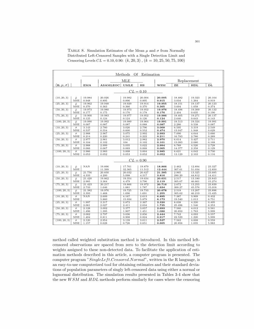
Table 8. Simulation Estimates of the Mean µ and σ from Normally
Distributed Left-Censored Samples with a Single Detection Limit and
Censoring Levels CL = 0.10, 0.90: (k, 20, 3) , (k = 10, 25, 50, 75, 100)
Methods Of Estimation
MLE Replacement(n, µ, σ) EMA ASAMLEOC UMLE HS WSM ZE HDL DL
CL = 0.10
(10, 20, 3) µMSE
19.9840.948
20.0260.895
19.9820.896
20.0040.895
20.0050.915
18.4823.034
19.3231.264
20.1640.919
(25, 20, 3) µMSE
19.9620.370
19.9480.363
19.9290.366
19.9140.370
19.9550.365
18.1513.694
19.1371.058
20.1230.374
(50, 20, 3) µMSE
19.9730.177
19.9800.175
19.9730.176
19.9520.178
19.9760.176
18.4962.404
19.3090.635
20.1220.190
(75, 20, 3) µMSE
19.9000.125
19.9830.124
19.9770.124
19.9520.126
19.9860.124
18.4052.646
19.2710.643
20.1370.143
(100, 20, 3) µMSE
19.9900.087
19.9920.087
19.9890.087
19.9640.088
19.9910.087
18.5132.286
19.3240.538
19.9910.087
(10, 20, 3) σMSE
3.1430.537
2.7800.554
3.0260.600
2.7960.552
3.0680.474
6.59513.047
3.3191.948
2.5490.629
(25, 20, 3) σMSE
2.9880.214
2.9670.220
3.0750.241
2.9920.222
2.9930.211
7.09016.783
4.6442.786
2.6660.289
(50, 20, 3) σMSE
2.9770.104
2.9610.102
3.012104
2.9820.102
2.9700.101
6.61413.083
3.4272.080
2.7110.168
(75, 20, 3) σMSE
2.9880.066
2.9990.067
3.0350.069
3.0220.068
2.9940.065
6.78914.377
4.5262.358
2.7280.129
(100, 20, 3) σMSE
2.9860.053
2.9830.052
3.0080.053
3.0040.052
2.9850.052
6.62113.129
4.0422.103
2.7300.116
CL = 0.90
(10, 20, 3) µMSE
NAN 19.89611.399
17.76132.365
19.87911.512
18.86612.444
2.462307.61
12.89451.034
23.32712.850
(25, 20, 3) µMSE
21.7564.333
20.8304.200
20.0325.098
20.6274.317
21.3853.816
2.965290.20
13.32544.812
23.68514.411
(50, 20, 3) µMSE
21.4202.985
19.8623.364
19.3544.479
19.6343.796
20.6312.119
2.517305.67
13.18046.661
23.84315.274
(75, 20, 3) µMSE
21.4232.733
20.2171.646
19.8661.881
19.9721.787
20.7161.634
2.672300.27
13.25545.576
23.83915.018
(100, 20, 3) µMSE
21.3822.393
19.9761.468
19.7251.696
19.7331.691
20.6781.255
2.518305.62
13.20746.219
23.89615.425
(10, 20, 3) σMSE
NAN 2.6095.860
4.16715.924
2.6135.879
6.8956.173
7.38719.540
3.9091.013
0.4326.751
(25, 20, 3) σMSE
1.9972.061
2.3172.027
2.8722.411
2.3672.034
2.3201.735
8.03825.496
4.2201.546
0.4956.353
(50, 20, 3) σMSE
2.1281.496
3.0021.395
3.3771.907
3.0571.451
2.6931.086
7.56020.850
4.0121.763
0.5615.999
(75, 20, 3) σMSE
2.0821.404
2.7970.811
3.0360.908
2.8560.824
2.4440.917
7.74222.529
4.0931.220
0.5575.999
(100, 20, 3) σMSE
2.1201.157
2.9540.628
3.1390.726
3.0110.651
2.5370.665
7.56320.856
4.0081.035
0.5595.983
method called weighted substitution method is introduced. In this method left-censored observations are spaced from zero to the detection limit according toweights assigned to these non-detected data. To facilitate the application of esti-mation methods described in this article, a computer program is presented. Thecomputer program ”SingleLeft.Censored.Normal”, written in the R language, isan easy-to-use computerized tool for obtaining estimates and their standard devia-tions of population parameters of singly left-censored data using either a normal orlognormal distribution. The simulation results presented in Tables 3-4 show thatthe new WSM and HDL methods perform similarly for cases where the censoring
301

levels is less than 50%. The new WSM method perform better than EMA andASAMLEOC methods for cases where the censoring levels is less than 50%. Forestimating the σ parameter the new WSM method perform better than the exist-ing methods for cases where the censoring levels is greater than or equal to 75%.Taken together, the suggested new WSM method appear to work best for nor-mally distributed censored samples, and lognormal versions of the estimator canbe obtained simply by taking natural logarithm of the data and the detection limit.
AcknowledgementsThe author is deeply indebted to the editor Professor Dr. Cem Kadilar and thereferees for their useful comments and recommendations which enhanced the clar-ity of the results of this work.
References
[1] Aboueissa A. A.and Stoline M. R. (2004). Estimation of the Mean and StandardDeviation from Normally Distributed Singly-Censored Samples, Environmetrics 15:659-673.
[2] Aboueissa A. A.and Stoline M. R. (2006). Maximum Likelihood Estimators of Popu-lation Parameters from Doubly-Left Censored Samples, Environmetrics 17: 811-826.
[3] Box G. E. P. and Cox D. R. (1964). An Analysis of Transformation (with Discussion),Journal of the Royal Statistical Society, Series B. 26(2): 211-252.
[4]Cohen A. C. JR. (1959). Simplified Estimators for the Normal Distribution WhenSamples Aare Singly Censored or Truncated, Technometrics 3: 217-237.
[5]Cohen A. C. (1991). Truncated and Censored Samples, Marcel Dekker, INC., NewYork.
[6]Dempster A. P., N. Laird M. and Rubin D. B. (1977). Maximum Likelihood fromIncomplete Data via the EM Algorithm, The Journal Of Royal Statistical Society B39: 1-38.
[7]El-Shaarawi A. H. and Dolan D. M. (1989). Maximum Likelihood Estimation of Wa-ter Concentrations from Censored Data, Canadian Journal of Fisheries and AquaticSciences 46: 1033-1039.
[8]El-Shaarawi A. H. and Esterby S. R. (1992). Replacement of Censored Observationsby a Constant: An Evaluation, Water Research 26(6): 835-844.
[9]Krishnamoorthy, K., Mallick, A. and Mathew, T. (2011). Inference for the lognormalmean and quantiles based on samples with nondetetcts, Atmos. Technomterics, 53:72-83.
[10]Kushner E.J. (1976). On Determining the Statistical Parameters for Pouplation Con-centration from a Truncated Data set, Atmos. Environ. 10: 975-979.
[11]Lagakos S. W., Barraj L. M. and De Gruttola V. (1988). Nonparametric Analysis ofTruncated Survival Data, With application to AIDS, Biometrika. 75, 3: 515-523.
[12]Gibbons, RD. (1994). Statistical Methods for Groundwater Monitoring, John Wileyand Sons, New York.
[13]Gilbert Richard O. (1987). Statistical Methods for Environmental Pollution Monitor-ing, Van Nostrand Reinhold: New York.
[14]Gilliom R. J. and Helsel D. R. (1986). Estimation of Distributional Parameters forCensored Trace Level Water Quality Data. I. Estimation Techniques, Water ResourcesRes. 22: 135-146.
[15]Gleit, A. (1985). Estimation for small normal data sets with Detection Limits, Envi-ron. Sci. Technol. 19: 1201-1206.
[16]Gupta A. K. (1952). Estimation of the Mean and Standard Deviation of a NormalPopulation from a Censored Sample, Biometrika 39: 260-237.
[17]Hass and Scheff (1990). Estimation of the averages in Truncated Samples, Environ-mental Science and Technology. 24: 912-919.
302

[18]Hald A.(1952). Maximum Likelihood Estimation of the Parameters of a Normal Dis-tribution which is Truncated at a Known Point, Scandinavian Actuarial journal. 32:119-134.
[19]Helsel D. R. and Gilliom R. J. (1986). Estimation of Distributional Parameters forCensored Trace Level Water Quality Data. II. Verification and application, WaterResources Res. 22: 147-155.
[20]Helsel D. R. and Hirsch R. M. (1988). Statistical Methods in Water Ressources,Elsevier: New York.
[21]Hyde J. (1977). Testing Survival under right-censoring and Left-Truncation, Biometrika.64: 225-230.
[22]Saw J. G. (1961). Estimation of the Normal Population Parameters Given a Type ICensored Sample, Biometrika 48: 367-377.
[23]Saw J. G. (1961b). The Bias of The Maximum Likelihood Estimates of the Locationand Scale Parameters Given a Type II Censored Normal Sample, Biometrika 48: 448-451.
[24]Schmee J., Gladstein D. and Nelson W. (1985). Confidence Limits of a NormalDistribution from Singly Censored Samples Using Maximum Likelihood, Technometrics27: 119-128.
[25]Schneider H. (1986). Truncated and Censored Samples from Normal Population,Marcel Dekker: New York.
[26]Shumway R. H. , Azari A. S. and Johnson P. (1989). Estimating Mean ConcentrationsUnder Transformation for Environmental Data With Detection Limit.,Technometrics.31: 347-357.
[27]Stoline Michael R. (1993). Comparison Oof Two Medians Using a Two-Sample Log-normal Model Iin Environmental Contexts, Environmetrics 4(3): 323-339.
[288]USEPA. (1989b). Statistical Analysis of Ground-Water Monitoring Data at RCRAFacilities, Interim Final Guidance. EPA/530-SW-89-026. Office of Solid Waste, U.S.Environmental Protection Agency: Washington, D.C.
[29]Wei-Yann Tsai (1990). Testing the Assumption of independent of Truncation Timeand Failure Time, Biometrika. 77, 1 : 169-177.
[30]Wolynetz, M. S. (1979). Maximum Likelihood Estimation from Confined and Censored
Normal Data, Applied Statistics. 28, 185-195.
303
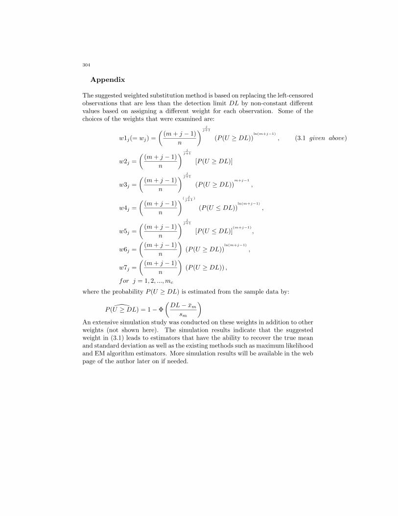
Appendix
The suggested weighted substitution method is based on replacing the left-censoredobservations that are less than the detection limit DL by non-constant differentvalues based on assigning a different weight for each observation. Some of thechoices of the weights that were examined are:
w1j(= wj) =
((m+ j − 1)
n
) jj+1
(P (U ≥ DL))ln(m+j−1)
, (3.1 given above)
w2j =
((m+ j − 1)
n
) jj+1
[P (U ≥ DL)]
w3j =
((m+ j − 1)
n
) jj+1
(P (U ≥ DL))m+j−1
,
w4j =
((m+ j − 1)
n
)(jj+1
)
(P (U ≤ DL))ln(m+j−1)
,
w5j =
((m+ j − 1)
n
) jj+1
[P (U ≤ DL)](m+j−1)
,
w6j =
((m+ j − 1)
n
)(P (U ≥ DL))
ln(m+j−1)
,
w7j =
((m+ j − 1)
n
)(P (U ≥ DL)) ,
for j = 1, 2, ...,mc
where the probability P (U ≥ DL) is estimated from the sample data by:
P (U ≥ DL) = 1− Φ
(DL− xm
sm
)
An extensive simulation study was conducted on these weights in addition to otherweights (not shown here). The simulation results indicate that the suggestedweight in (3.1) leads to estimators that have the ability to recover the true meanand standard deviation as well as the existing methods such as maximum likelihoodand EM algorithm estimators. More simulation results will be available in the webpage of the author later on if needed.
304

Table 9. Simulation Estimates of the Mean µ and σ from Normally
Distributed Left-Censored Samples with a Single Detection Limit and
Censoring Levels CL = 0.75, 0.90: (k, 25, 10) , (k =10, 25, 50, 75, 100)
Methods Of Estimation(n, µ, σ) MLE W1j(= Wj) W2j W3j W4j W5j W6j W7j
CL = 0.75
(10, 25, 10) µMSE
26.82034.258
24.23412.401
23.25216.047
19.32951.433
11.108194.777
10.741205.259
21.51521.974
22.40215.600
(25, 25, 10) µMSE
26.06314.436
23.4656.016
20.81022.861
13.064148.885
10.320216.079
10.235218.583
19.89930.475
22.4339.668
(50, 25, 10) µMSE
25.4936.912
24.2065.299
19.84230.481
10.692206.662
9.706234.184
9.689234.705
19.33935.300
21.5447.859
(75, 25, 10) µMSE
25.1485.072
24.5215.233
19.29635.658
9.883229.296
9.493240.630
9.487240.824
18.92040.013
21.6258.410
(100, 25, 10) µMSE
24.9803.789
24.1134.305
18.71442.200
9.571238.248
9.416242.978
9.413243.065
18.99738.541
22.9706.051
(10, 25, 10) σMSE
7.49022.999
8.9213.664
8.5364.216
11.1436.978
16.35444.455
16.58647.441
10.1112.020
3.02351.492
(25, 25, 10) σMSE
8.78211.516
10.1681.413
9.3425.342
14.90227.034
16.56044.618
16.61245.296
11.2665.969
10.3797.088
(50, 25, 10) σMSE
9.4515.080
9.7450.576
11.8733.077
15.96036.846
16.52243.411
16.53243.540
12.4755.094
11.9874.726
(75, 25, 10) σMSE
9.7263.637
9.9120.314
11.2672.292
16.24539.594
16.46342.298
16.46742.344
11.6114.972
11.9455.237
(100, 25, 10) σMSE
9.9502.791
10.4861.468
11.7324.555
16.39741.318
16.48442.428
16.48542.448
12.4643.102
10.9972.250
CL = 0.90
(10, 25, 10) µMSE
24.891108.321
24.21599.875
22.568114.827
7.982387.340
5.174393.543
4.045439.447
20.009121.432
20.099132.093
(25, 25, 10) µMSE
27.91844.648
23.32742.724
20.05045.861
12.317191.703
5.044398.446
4.918403.496
18.74848.107
20.92741.091
(50, 25, 10) µMSE
24.60631.013
23.93829.925
18.52652.094
8.797289.135
4.245430.836
4.214432.141
17.93759.028
20.84431.088
(75, 25, 10) µMSE
25.96717.901
23.98316.502
16.58478.491
5.541382.210
4.485420.910
4.465421.758
15.98388.275
20.56921.601
(100, 25, 10) µMSE
24.94417.655
23.89616.520
16.54478.921
5.135398.059
4.222431.778
4.213432.136
16.18884.747
21.69020.197
(10, 25, 10) σMSE
8.58752.124
9.07150.071
8.67255.982
12.01467.803
13.32284.007
13.36658.602
14.07155.341
13.51052.762
(25, 25, 10) σMSE
7.78422.567
9.77115.847
9.58524.087
11.90616.094
16.56044.618
16.61245.296
12.64725.442
12.99323.087
(50, 25, 10) σMSE
9.91513.288
9.96410.487
10.73011.522
12.51013.951
12.68714.890
12.99713.944
11.60415.604
12.10612.106
(75, 25, 10) σMSE
9.2078.208
10.1565.371
11.4157.468
12.6569.784
12.9779.332
12.9849.373
10.9388.034
11.0487.997
(100, 25, 10) σMSE
9.7557.583
10.1435.264
11.5446.514
12.4237.486
12.6968.591
12.6998.606
11.4796.479
11.0298.029
305

Table 10. Simulation Estimates of the Mean µ and σ from Normally
Distributed Left-Censored Samples with a Single Detection Limit and
Censoring Levels CL = 0.15, 0.50: (k, 10, 5) , (k = 10, 25, 50, 75, 100)
Methods Of Estimation(n, µ, σ) MLE W1j(= Wj) W2j W3j W4j W5j W6j W7j
CL = 0.15
(10, 10, 5) µMSE
10.0132.669
10.3272.617
10.3882.988
11.0722.899
9.0013.120
9.1053.195
10.7043.560
11.2643.626
(25, 10, 5) µMSE
10.0471.013
10.0731.008
10.5601.788
9.6611.843
9.3261.848
9.0341.901
10.5441.196
10.7031.934
(50, 10, 5) µMSE
9.9640.492
10.0840.490
10.2860.553
9.5700.804
9.3800.638
9.2940.701
10.3630.781
10.5650.739
(75, 10, 5) µMSE
9.9390.373
10.1640.367
10.3720.426
9.6180.621
9.5850.438
9.2750.509
10.3570.470
10.4700.478
(100, 10, 5) µMSE
9.9910.255
10.0820.270
10.2980.334
9.6540.375
9.5420.416
9.3430.493
10.1650.273
10.3800.326
(10, 10, 5) σMSE
4.8561.703
4.6091.544
4.2411.973
4.0652.164
5.9742.218
6.7462.228
4.2211.986
4.2442.507
(25, 10, 5) σMSE
4.8860.617
4.7720.690
4.3560.842
5.2090.973
5.5200.908
5.7280.937
4.5220.690
4.4090.798
(50, 10, 5) σMSE
4.9520.329
4.8850.302
4.4040.585
5.4560.604
5.5130.698
5.7430.599
4.2700.603
4.4170.957
(75, 10, 5) σMSE
5.0450.237
4.8290.293
4.4820.434
5.4960.450
5.5530.500
5.7290.564
4.6450.375
4.5100.609
(100, 10, 5) σMSE
4.9230.161
4.7720.189
4.4120.458
5.4310.354
5.4490.377
5.7930.386
4.5890.306
4.4300.414
CL = 0.50
(10, 10, 5) µMSE
10.0933.433
10.1142.506
10.4902.339
9.2453.189
6.89710.452
6.85310.724
9.7063.213
10.6553.233
(25, 10, 5) µMSE
10.2281.533
9.9750.827
10.5931.230
7.8735.163
7.1698.352
7.1628.392
9.5600.889
10.4450.989
(50, 10, 5) µMSE
10.0200.711
9.9690.561
10.4930.677
7.2008.130
6.9809.288
6.9799.288
9.6200.608
10.4640.664
(75, 10, 5) µMSE
10.0540.522
9.7790.517
10.5730.547
7.0788.670
7.0318.931
7.9578.652
9.4830.690
10.9500.472
(100, 10, 5) µMSE
10.0290.339
9.8270.366
10.4690.466
6.9969.112
6.9829.194
6.9829.196
9.4650.627
10.4820.769
(10, 10, 5) σMSE
4.4642.744
4.3101.864
3.7413.279
4.6332.321
7.0745.166
7.1155.343
4.3702.190
4.1792.320
(25, 10, 5) σMSE
4.6591.280
4.5990.668
3.9681.407
6.5022.879
7.2005.184
7.2075.217
4.7050.998
10.5341.093
(50, 10, 5) σMSE
4.9340.586
4.8660.267
4.1180.933
7.0824.565
7.2935.565
7.2945.436
9.5200.703
10.9640.864
(75, 10, 5) σMSE
4.8680.427
4.8680.179
4.1160.895
7.2115.021
7.2575.215
7.9466.012
4.6580.258
4.2420.683
(100, 10, 5) σMSE
4.9240.273
4.9320.118
4.1480.800
7.2765.275
7.2905.337
7.2905.338
5.3110.216
4.2610.617
306

Table 11. Simulation Estimates of the Mean µ and σ from Normally
Distributed Left-Censored Samples with a Single Detection Limit and
Censoring Levels CL = 0.10, 0.90: (k, 20, 3) , (k = 10, 25, 50, 75, 100)
Methods Of Estimation(n, µ, σ) MLE W1j(= Wj) W2j W3j W4j W5j W6j W7j
CL = 0.10
(10, 20, 3) µMSE
20.0260.895
20.0080.881
19.8810.892
19.0671.319
18.4883.016
18.4823.034
19.7520.913
19.3750.870
(25, 20, 3) µMSE
19.9480.363
19.9370.353
19.7620.408
18.8631.735
18.1513.693
18.1513.694
19.4740.538
19.6830.483
(50, 20, 3) µMSE
19.9800.176
19.9840.172
19.7990.217
18.7361.794
18.4962.404
17.9682.725
19.6720.238
19.7540.282
(75, 20, 3) µMSE
19.9830.124
19.9900.122
19.7810.175
18.5312.277
18.4052.646
17.9982.763
19.6670.0.238
19.8730.195
(100, 20, 3) µMSE
19.9920.087
19.9990.087
19.7830.139
18.5592.157
18.5132.286
18.09214.109
19.7610.147
19.0720.185
(10, 20, 3) σMSE
2.7800.554
3.0260.432
2.7890.455
4.2182.324
6.57912.932
6.59513.047
3.2040.543
2.7720.493
(25, 20, 3) σMSE
2.9670.220
2.9530.173
3.2740.292
5.3116.297
7.09016.777
7.39015.638
3.3670.427
3.2450.258
(50, 20, 3) σMSE
2.9610.102
2.9280.081
3.2850.187
5.9519.016
6.61413.083
7.02512.573
3.3480.218
2.7900.276
(75, 20, 3) σMSE
2.9990.067
2.9600.054
3.3590.204
6.44712.022
6.78914.377
6.99312.948
3.4080.241
3.2090.187
(100, 20, 3) σMSE
2.9830.052
2.9450.045
3.3650.194
6.49212.238
6.62113.129
6.90412.839
3.4050.225
2.7890.098
CL = 0.90
(10, 20, 3) µMSE
19.39815.410
18.99316.107
17.85917.703
14.98230.444
5.676282.441
4.462307.606
12.83651.858
13.90847.054
(25, 20, 3) µMSE
20.8304.200
18.7596.295
17.9838.054
12.46777.596
11.05083.965
13.96692.837
11.65872.274
13.13357.946
(50, 20, 3) µMSE
19.8623.364
18.6993.109
15.7955.895
10.2778.973
6.53712.948
6.51756.666
13.12510.102
12.04241.033
(75, 20, 3) µMSE
20.2171.646
18.6492.017
16.9723.896
9.68311.874
8.37513.874
7.04715.266
13.19611.551
12.97216.801
(100, 20, 3) µMSE
19.9763.706
19.2744.003
14.2808.604
14.16816.173
8.52321.403
7.51823.619
13.13833.287
14.97349.818
(10, 20, 3) σMSE
2.6095.860
3.5466.027
4.0136.627
5.5467.182
7.47015.271
7.38716.539
4.9755.048
4.9986.192
(25, 20, 3) σMSE
2.3172.027
3.4022.377
3.8693.094
5.6784.289
5.6787.286
6.03811.494
4.8123.750
5.09110.700
(50, 20, 3) σMSE
2.9361.392
3.0781.973
4.9483.275
5.8265.749
6.5539.788
6.56010.849
5.3298.188
4.9587.854
(75, 20, 3) σMSE
2.7972.811
3.3062.913
3.9724.870
8.52210.611
7.73817.492
6.80315.529
5.02810.722
6.1459.321
(100, 20, 3) σMSE
2.5944.628
3.5145.023
6.0146.286
7.37813.307
7.56215.009
7.56314.721
6.2358.517
6.6637.452
307

Hacettepe Journal of Mathematics and StatisticsVolume 43 (2) (2014), 309 – 322
Parameter estimation by anfis where dependentvariable has outlier
Turkan Erbay Dalkılıc a ∗, Kamile Sanlı Kula b †, and Aysen Apaydın c ‡
Abstract
Regression analysis is investigation the relation between dependent andindependent variables. And, the degree and functional shape of this re-lation is determinate by regression analysis. In case that dependentvariable has outlier, the robust regression methods are proposed tomake smaller the effect of the outlier on the parameter estimates. Inthis study, an algorithm has been suggested to define the unknownparameters of regression model, which is based on ANFIS (AdaptiveNetwork based Fuzzy Inference System). The proposed algorithm, ex-pressed the relation between the dependent and independent variablesby more than one model and the estimated values are obtained byconnected this model via ANFIS. In the solving process, the proposedmethod is not to be affected the outliers which are to exist in dependentvariable. So, to test the activity of the proposed algorithm, estimatedvalues obtained from this algorithm and some robust methods are com-pared.
Keywords: Adaptive network, fuzzy inference, robust regression.
2000 AMS Classification: 62J05, 62K25
aDepartment of Statistics and Computer Science, Faculty of Science, Karadeniz Technical
University, Trabzon, Turkey.∗Email: [email protected] of Mathematics, Faculty of Sciences and Arts, Ahi Evran University, Kirsehir,
Turkey†Email: [email protected] of Statistics, Faculty of Science, Ankara University, 06100, Tandogan, Ankara,
Turkey‡Email: [email protected]

T. E. Dalkılıc et al.
1. Introduction
In a regression analysis, it is assumed that the observations come from a sin-gle class in a data cluster and the simple functional relationship between thedependent and independent variables can be expressed using the general model;Y = f (X) + ε . However; a data set may consist of a combination of observationsthat have different distributions that are derived from different clusters. Whenfaced with issues of estimating a regression model for fuzzy inputs that have beenderived from different distributions, this regression model has been termed the
’switching regression model’ and it is expressed with Y L = fL(X)+εL (L =p∏i=1
li).
Here li indicates the class number of each independent variable and p is indicativeof the number of independent variables [18, 19, 21]. In case that, the class numbersof the data and the number of the independent variables are more than two, si-multaneously the numbers of sub-models are increased. At this stage, the methodattempts to utilize the neural networks, which are intended to solve complex prob-lems and systems. When faced with issues in which the data belong to an indefiniteor fuzzy class, the neural network, termed the adaptive network, is used for es-tablishing the regression model. In this study, adaptive networks have been usedto construct a model that has been formed by gathering obtained models. Thereare methods that suggest the class numbers of independent variables heuristically.Alternatively, in defining the optimal class number of independent variables, theuse of suggested validity criterion for fuzzy clustering has been aimed. There aremany studies on the use of the adaptive network for parameter estimation. In astudy by Chi-Bin, C. and Lee, E. S. a fuzzy adaptive network approach was estab-lished for fuzzy regression analysis [4] and it was studied on both fuzzy adaptivenetworks and the switching regression model [5]. Jang, J. R. studied the adaptivenetworks based on a fuzzy inference system [16]. In a study of Takagi, T. andSugeno, M., the method for identifying a system using it’s input-output data waspresented [23]. James, P. D. and Donalt, W., were studied fuzzy regression usingneural networks [15]. In a study by Cichocki, A. and Unbehauen, R., the differentneural networks for optimization were explained [2]. There are different studiesabout fuzzy clustering and the validity criterion. In the study of Mu-Song, C. andWang, S.W. the analysis of fuzzy clustering was done for determining fuzzy mem-berships and in this study a method was suggested for indicating the optimal classnumbers that belong to the variables [20]. Bezdek, J.C. has conducted importantstudies on the fuzzy clustering topic [1]. One such study is by Hathaway R.J. andBezdek J.C. were studied on switching regression and fuzzy clustering [7]. In 1991,Xie, X.L. and Beni, G. suggested a validity criterion for fuzzy clustering [24]. Inthis study we used the Xie-Beni validity criterion for determining optimal classnumbers. Over the years, the least squares method(LSM) has commonly beenused for the estimation of regression parameters. If a data set conforms to LSMassumptions, LSM estimates are known to be the best. However, if outliers exist inthe data set, the LSM can yield bad results. In the conventional approach, outliersare removed from the data set, after which the classical method can be applied.However, in some research, these observations are not removed from the data set.In such cases, robust methods are preferred to the LSM [17]. The remainder of
310

Parameter estimation by anfis where dependent variable has outlier
the paper is organized as follows. Section 2 explores the fuzzy if-then rules andthe use of these rules will be introduced using adaptive networks for analysis. InSection 3 an algorithm for parameter estimation based ANFIS is given.In Section4, we provide definitions of M methods of Huber, Hampel, Andrews and Tukey,which are commonly used in the literature. In Section 5, a numerical applicationexamining the work and validity of the suggested algorithm as well as a compar-ison of the algorithm with these robust methods and LSM is provided.In the lastpart, a discussion and conclusion are provided.
2. ANFIS: Adaptive Network based Fuzzy Inference System
The most popular application of fuzzy methodology is known as fuzzy inferencesystems. This system forms a useful computing framework based on the concepts offuzzy set theory, fuzzy reasoning and fuzzy if-then rules. Fuzzy inference systemsusually perform on input-output relation, as in control applications where theinputs correspond to system state variables, and the outputs are control signals[3, 5, 16]. The fuzzy inference system is a powerful function approximater. Thebasic structure of a fuzzy inference system consist of five conceptual components;arule base which contains a selection of fuzzy rules, a database which defines themembership functions of the fuzzy sets used in the fuzzy rules, a decision-makingunit which performs inference operations on the rules, a fuzzification interfacewhich transforms the crisp inputs into degrees of match with linguistic values, anda defuzzification interface which transform the fuzzy results of the inference intoa crisp output [3, 15, 16]. The adaptive network used to estimate the unknownparameters of regression model is based on fuzzy if-then rules and fuzzy inferencesystem. When issues of estimating a regression model to fuzzy inputs from differentdistributions arose, the Sugeno Fuzzy Inference System is appropriate and theproposed fuzzy rule in this case is indicated as
RL = If ;(x1 = FL1 and x2 = FL2 and . . . xp = FLp
).
Then; Y = Y L = cL0 + cL1 x1 + ...+ cLp xp.
Here, FLi stands for fuzzy cluster and Y L stands for system output accordingto the RL rule [16, 23].
The weighted mean of the models obtained according to fuzzy rules is the outputof Sugeno Fuzzy Inference System and a common regression model for data fromdifferent classes is indicated with this weighted mean as follows,
Y =
m∑L=1
wLY L
m∑L=1
wL.
Here; wL weight is indicated as,
wL =
p∏
i=1
µFLi (xi).
311

T. E. Dalkılıc et al.
µFLi
(xi) is a membership function defined on the fuzzy set FLi , and m is fuzzy
rule number [13, 14].Neural networks that enable the use of fuzzy inference systems for fuzzy re-
gression analysis is known as adaptive network and called ANFIS. An adaptivenetwork is a multilayer feed forward network in which each node performs a par-ticular function on incoming signals as well as a set of parameters pertaining to thisnode. The formulas for the node functions may wary from node to node and thechoice of each node function depends on the overall input-output function of thenetwork. Neural networks are used to obtain a good approach to regression func-tions and were formed via neural and adaptive network connections consistingoffive layers [4, 12− 14, 15].
Fuzzy rule number of the system depends on numbers of independent variablesand fuzzy class number forming independent variables. When independent variablenumber is indicated with p and if the fuzzy class number associated with eachvariable is indicated by li (i = 1, ..., p), the fuzzy rule number indicated by
L =
p∏
i=1
li.
To illustrate how a fuzzy inference system can be represented by ANFIS, letus consider the following example. Suppose a data set has two-dimensional inputX = (x1, x2). For input x1, there are two fuzzy sets ”tall” and ”short” and forinput x2, three fuzzy set ”thin”, ”normal” and ”fat”. In this case a fuzzy inferencesystem contains the following six rules:
R1 : If(x1 is tall and x2 is thin), then; (Y 1 = c10 + c11x1 + c12x2),
R2 : If(x1 is tall and x2 is normal), then; (Y 2 = c20 + c21x1 + c22x2),
R3 : If(x1 is tall and x2 is fat), then; (Y 3 = c30 + c31x1 + c22x2),
R4 : If(x1 is short and x2 is thin), then; (Y 4 = c40 + c41x1 + c42x2),
R5 : If(x1 is short and x2 is normal), then; (Y 5 = c50 + c51x1 + c52x2),
R6 : If(x1 is short and x2 is fat), then; (Y 6 = c60 + c61x1 + c62x2).
This fuzzy system is represented by the ANFIS as shown in Figure 1. Thefunctions of each node in Figure 1 defined as follows.
Layer 1: The output of node h in this layer is defined by the membershipfunction on Fh
f1,h = µFh(x1) for h = 1, 2
f1,h = µFh(x2) for h = 3, 4, 5
where fuzzy cluster related to fuzzy rules are indicated with F1, F2, ..., Fh andµFh
is the membership function relates to Fh. Different membership functions arecan be define for Fh. In this example, the Gaussian membership function will beused whose parameters can be represented by vh, σh.
312

Parameter estimation by anfis where dependent variable has outlier
]
Figure 1. The ANFIS architecture
µFh(x1) = exp
[−(x1 − vhσh
)2]
for h = 1, 2
µFh(x2) = exp
[−(x2 − vhσh
)2]
for h = 3, 4, 5.
The parameter set vh, σh in this layer is referred to as the premise parameters.Layer 2: Each nerve in the second layer has input signals coming from the first
layer and they are defined as multiplication of these input signals. This multipliedoutput forms the firing strength wl for rule l:
f2,1 = w1 = µF1(x1)× µF3(x2),
f2,2 = w2 = µF1(x1)× µF4
(x2),
f2,3 = w3 = µF1(x1)× µF5(x2),
f2,4 = w4 = µF2(x1)× µF3
(x2),
f2,5 = w5 = µF2(x1)× µF4
(x2),
f2,6 = w6 = µF2(x1)× µF5(x2).
Layer 3: The output of this layer is a normalization of the outputs of thesecond layer and nerve function is defined as
f3,L = wL =wL
6∑L=1
wL.
313

T. E. Dalkılıc et al.
Layer 4: The output signals of the fourth layer are also connected to a functionand this function is indicated with
f4,L = wLY L
where, Y L stands for conclusion part of fuzzy if-then rule and it is indicated with
Y L = cL0 + cL1 x1 + cL2 x2,
where cLi are fuzzy numbers and stands for posteriori parameters.Layer 5: There is only one node which computes the overall output as the
summation of all the incoming signals
f5,1 = Y =
6∑
L=1
wLY L.
3. An Algorithm for Parameter Estimation Based ANFIS
The estimation of parameters with an adaptive network is based on the principleof the minimizing of error criterion. There are two significant steps in the processof estimation. First, we must determine the a priori parameter set characterizingthe class from which the data comes and then update these parameters within theprocess. The second step is to determine a posteriori parameters belonging to theregression models to be formed. The process of determining parameters for theswitching regression model begins with determining class numbers of independentvariables and a priori parameters [6]. The algorithm related to the proposedmethod for determining the switching regression model in the case of independentvariables coming from a normal distribution is defined as follows.
Step 1: Optimal class numbers related to the data set associated with theindependent variables are determined. Optimal value of class number li, (li = 2,li= 3 . . . li= max) can be obtained by minimizing the fuzzy clustering validityfunction Si. This function is expressed by
Si =
1n
li∑i=1
n∑j=1
( uij)m ‖vi − xj‖2
mini 6=j‖vi − vj‖2
.
As it can be seen in this statement, cluster centers, which are well-separatedproduce a high value of separation such that a smaller Si value is obtained. Whenthe lowest Si value is observed, class number (li) with the lowest value is definedas an optimal class number.
Step 2: A priori parameters are determined. Spreading is determined intu-itively according to the space in which input variables gain value and to the fuzzyclass numbers of the variables. Center parameters are based on the space in whichvariables gain value and fuzzy class numbers and it is defined by
314

Parameter estimation by anfis where dependent variable has outlier
vi = (minXi) +max (Xi)−min (Xi)
li − 1(i− 1) , i = 1, 2, ..., p.
Step 3: wL weights are counted which are used to form matrix B to be usedin counting the a posteriori parameter set. L is the fuzzy rule number. The wL
weights are outputs of the nerves in the third layer of the adaptive network, andthey are counted based on a membership function related to the distribution familyto which independent variable belongs. Nerve functions in the first layer of theadaptive network are defined by
f1,h = µFh(xi) h = 1, 2, ...,
p∑
i=1
li.
µFh(xi) is called the membership function. Here, when the normal distribu-
tion function which has the parameter set of vh, σh is considered, membershipfunctions are defined as
µFh(xi) = exp
[−(xi − vhσh
)2].
From the defined membership functions, membership degrees related to each classforming independent variables are determined. The wL weights are indicated as
wL = µFL(xi).µFL
(xj).
They are obtained via mutual multiplication of membership degrees at an amountdepending on the number of independent variables and the fuzzy class numbersof these variables. wL weight is a normalization of the weight defined as wL andthey are counted with
wL =wL
m∑L=1
wL.
Step 4: On the condition that the independent variables are fuzzy and thedependent variables are crisp, a posteriori parameter set cLi = (aLi , b
Li ) is obtained
as crisp numbers in the shape of, cLi = aLi (i = 1, ..., p). In that condition,
Z =(BTB
)−1BTY equation is used to determine the a posteriori parameter
set. Here B is the data matrix which is weighted by membership degree and itsdimension is [(p+ 1)×m× n], Y dependent variable vector and Z is posteriorparameter vector which is defined by
Z =[a1
0, ..., am0 , a
11, ..., a
m1 , ..., a
1p, ..., a
mp
]T
Step 5: By using a posteriori parameter set cLi = aLi obtained in Step 4, theregression model indicated by
Y L = cL0 + cL1 x1 + cL2 x2 + ...+ cLp xp
315

T. E. Dalkılıc et al.
are constituted. Setting out from the models and weights specified in Step 1, theestimation values are obtained using
Y =m∑
L=1
wLY L.
Step 6: The error related to model is counted as
εk =
n∑
k=1
(yk − yk)2.
If ε < φ, then the a posteriori parameters have been obtained as parameters ofregression models to be formed, and the process is determinate. If ε < φ, then,Step 6 begins. Here φ, is a law stable value determinated by the decision maker.Step 7: Central a priori parameters specified in Step 2 are updated with
v′i = vi ± t
in a way that it increases from the lowest value to the highest and it decreasesfrom the highest value to the lowest. Here, t is the size of the step;
t =max (xji)−min (xji)
aj = 1, 2, ..., n; i = 1, 2, ..., p
and a is a stable value, which is determinant by the size of the step, and is thereforean iteration number.
Step 8: Estimations for each a priori parameter obtained by change and theerror criteria related to these estimations are counted. The lowest of the errorcriterion is defined. A priori parameters giving the lowest error specified, and theestimation obtained via the models related to these parameters is taken as output.
In the proposed algorithm, the estimated values which are obtained from thefuzzy adaptive network are not to be affected by the outliers that may exist inthe dependent variable. This is because in this algorithm, all of the independentvariables are weighted. Consequently, the proposed method has a robust method’sproperties, and, it is comparable to robust methods that are commonly used inliterature.
4. M methods
The classical LSM is widely used in regression analysis because computing itsestimate is easy and traditional. However, least square estimators are very sensitiveto outliers and to deviations from basic assumptions of normal theory [11, 25]. Theimportance of eachobservation should therefore be recognized, and the data shouldbe tested in detail whenit is analyzed. This is important because sometimes evena single observation can changethe value of the parameter estimates, and omittingthis observation from the data maylead to totally different estimates. If thereexist outliers in the data set, robust methods are preferred to estimate parametervalues [22]. Now, we discuss the widely used methods of the Huber, Hampel,Andrews and Tukey M estimators. The M estimator utilizes minimizing of residual
316

Parameter estimation by anfis where dependent variable has outlier
functions much more thanminimizing the sum of the squared residuals. Regressioncoefficients are obtained by theminimizing sum:
(4.1)
n∑
i=1
ρ
yi −
p∑
j=1
xij βj
d
.
By taking the first partial derivative of the sum in Equation (4.1) with respect
to each βj and setting it to zero, it may be found regression coefficient that pequations:
n∑
i=1
xijΨ
yi −
p∑
j=1
xij βj
d
= 0 j = 1, 2, ..., p
where Ψ(z) = ρ′(z). When the data contains outliers, standard deviations are not
good measures of variability, and other robust measures of variability are thereforerequired. One robust measure of variability is d. In the case where ri is theresidual of ith observation, d = median |ri −median (ri)|0.6745, i = 1, 2, ..., n.Therefore, the standardized residuals may be defined as z = rid. Inaddition
ri = yi −p∑j=1
xij βj .
Huber’s Ψ function is defined as:
Ψ (z) =
−k z < −kz |z| ≤ kk z > k
with k=1.5.The Hampel Ψ function is defined as:
Ψ(z) =
|z| 0 < |z| ≤ aasgn(z) a < |z| ≤ b
a(c−|z|c−b
)sgn(z) b < |z| ≤ c
0 c < |z|
sgn(z) =
+1 z > 00 z = 0−1 z < 0
Reasonably good values of the constants are a = 1.7, b = 3.4 and c = 8.5.Andrews (sine estimate) Ψ function is defined as
Ψ (z) =
sin (zk) |z| ≤ kπ
0 |z| > kπ
with k =1.5 or k = 2.1.The Tukey (biweight estimate) Ψ function is defined as:
Ψ (z) =
(z(
1− (zk)2)2)
|z| ≤ k0 |z| > k
with k = 5.0 or 6.0 [8− 11].
317
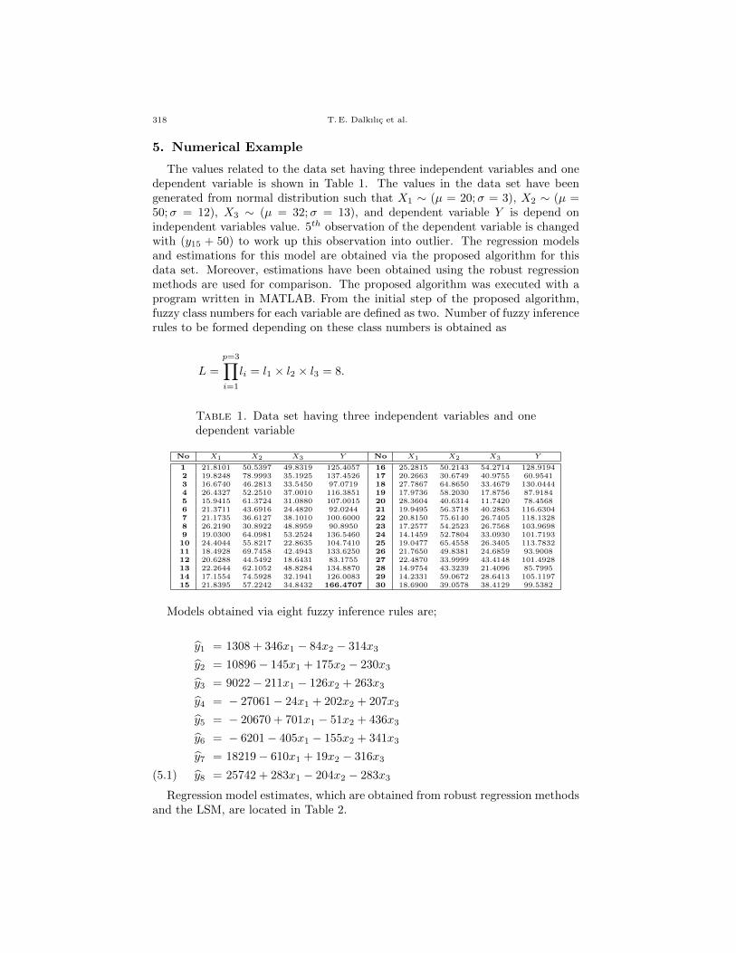
T. E. Dalkılıc et al.
5. Numerical Example
The values related to the data set having three independent variables and onedependent variable is shown in Table 1. The values in the data set have beengenerated from normal distribution such that X1 ∼ (µ = 20;σ = 3), X2 ∼ (µ =50;σ = 12), X3 ∼ (µ = 32;σ = 13), and dependent variable Y is depend onindependent variables value. 5th observation of the dependent variable is changedwith (y15 + 50) to work up this observation into outlier. The regression modelsand estimations for this model are obtained via the proposed algorithm for thisdata set. Moreover, estimations have been obtained using the robust regressionmethods are used for comparison. The proposed algorithm was executed with aprogram written in MATLAB. From the initial step of the proposed algorithm,fuzzy class numbers for each variable are defined as two. Number of fuzzy inferencerules to be formed depending on these class numbers is obtained as
L =
p=3∏
i=1
li = l1 × l2 × l3 = 8.
Table 1. Data set having three independent variables and onedependent variable
No X1 X2 X3 Y No X1 X2 X3 Y
1 21.8101 50.5397 49.8319 125.4057 16 25.2815 50.2143 54.2714 128.91942 19.8248 78.9993 35.1925 137.4526 17 20.2663 30.6749 40.9755 60.95413 16.6740 46.2813 33.5450 97.0719 18 27.7867 64.8650 33.4679 130.04444 26.4327 52.2510 37.0010 116.3851 19 17.9736 58.2030 17.8756 87.91845 15.9415 61.3724 31.0880 107.0015 20 28.3604 40.6314 11.7420 78.45686 21.3711 43.6916 24.4820 92.0244 21 19.9495 56.3718 40.2863 116.63047 21.1735 36.6127 38.1010 100.6000 22 20.8150 75.6140 26.7405 118.13288 26.2190 30.8922 48.8959 90.8950 23 17.2577 54.2523 26.7568 103.96989 19.0300 64.0981 53.2524 136.5460 24 14.1459 52.7804 33.0930 101.719310 24.4044 55.8217 22.8635 104.7410 25 19.0477 65.4558 26.3405 113.783211 18.4928 69.7458 42.4943 133.6250 26 21.7650 49.8381 24.6859 93.900812 20.6288 44.5492 18.6431 83.1755 27 22.4870 33.9999 43.4148 101.492813 22.2644 62.1052 48.8284 134.8870 28 14.9754 43.3239 21.4096 85.799514 17.1554 74.5928 32.1941 126.0083 29 14.2331 59.0672 28.6413 105.119715 21.8395 57.2242 34.8432 166.4707 30 18.6900 39.0578 38.4129 99.5382
Models obtained via eight fuzzy inference rules are;
y1 = 1308 + 346x1 − 84x2 − 314x3
y2 = 10896− 145x1 + 175x2 − 230x3
y3 = 9022− 211x1 − 126x2 + 263x3
y4 = − 27061− 24x1 + 202x2 + 207x3
y5 = − 20670 + 701x1 − 51x2 + 436x3
y6 = − 6201− 405x1 − 155x2 + 341x3
y7 = 18219− 610x1 + 19x2 − 316x3
y8 = 25742 + 283x1 − 204x2 − 283x3(5.1)
Regression model estimates, which are obtained from robust regression methodsand the LSM, are located in Table 2.
318

Parameter estimation by anfis where dependent variable has outlier
Table 2. The estimation of regression parameters
Constant β1 β2 β3
LMS −10.4360 1.0404 1.2420 0.9412Huber 3.0366 0.8125 1.0329 1.0085Hampel 5.5338 0.7794 0.9778 1.0412Tukey 5.3224 0.8127 0.9625 1.0563
Andrews 5.2896 0.7775 0.9809 1.0430
The weights related to the observations that are used in estimation methodsfor regression models, are located in Table 3. The weights for robust methodsare expression of that observation’s effect on one model for each of the outlierobservations of the robust method. On the other hand, weight obtained fromthe network is an expression of that observation’s effect on more than one model,which are expressed in Equation (5.1). For this reason, eight different weights,which are called membership degrees of observation, are located in Table 3.
Table 3. The weight related to observation for all methods
No
LM
S
Huber
Ham
pel
Tukey
Andrews
The membership degrees of the observation to belong to the modelsin Equation (5.1)
w1 w2 w3 w4 w5 w6 w7 w81 1 1 1 0.9892 0.4710 0.2558 0.8399 0.1927 0.6327 0.2563 0.8714 0.1931 0.63412 1 1 1 0.9274 0.4632 0.1331 0.1553 0.6541 0.7634 0.1323 0.1544 0.6504 0.75903 1 1 1 0.9704 0.4713 0.4513 0.4688 0.2568 0.2667 0.4431 0.4603 0.2521 0.26194 1 1 1 0.9996 0.4752 0.2955 0.3919 0.2492 0.3305 0.3017 0.4001 0.2544 0.33745 1 1 1 0.9068 0.4545 0.2619 0.2287 0.4029 0.3518 0.2564 0.2239 0.3944 0.34446 1 1 1 0.9812 0.4702 0.9279 0.5080 0.4451 0.2437 0.9283 0.5082 0.4453 0.24387 1 0.9901 1 0.9383 0.4559 0.6285 0.9008 0.1891 0.2710 0.6283 0.9005 0.1890 0.27098 1 0.2780 0.1984 0 0.1023 0.1777 0.5464 0.0367 0.1128 0.1813 0.5573 0.0374 0.11509 1 1 1 0.9555 0.4685 0.1053 0.4404 0.1939 0.8109 0.1044 0.4365 0.1922 0.803710 1 1 1 0.9729 0.4692 0.5702 0.2784 0.6084 0.2971 0.5774 0.2820 0.6161 0.300911 1 1 1 0.9853 0.4732 0.1575 0.3079 0.4207 0.8225 0.1557 0.3045 0.4160 0.813412 1 1 1 0.9794 0.4728 0.9492 0.3440 0.4818 0.1746 0.9468 0.3431 0.4806 0.174213 1 1 1 0.9999 0.4758 0.1794 0.5488 0.2896 0.8859 0.1801 0.5510 0.2908 0.889514 1 1 1 0.9917 0.4754 0.1503 0.1419 0.5525 0.5216 0.1478 0.1396 0.5435 0.513215 1 0.0793 0 0 0 0.4992 0.5684 0.5843 0.6652 0.5004 0.5697 0.5856 0.666816 1 1 1 0.9371 0.4691 0.1247 0.5603 0.0919 0.4131 0.1267 0.5694 0.0934 0.419817 1 0.1292 0 0 0 0.5070 0.8905 0.1032 0.1812 0.5050 0.8869 0.1027 0.180418 1 1 1 0.8298 0.4345 0.1445 0.1493 0.2798 0.2891 0.1483 0.1532 0.2872 0.296719 1 0.5182 0.7229 0.6013 0.3816 0.5293 0.1817 0.6608 0.2268 0.5224 0.1793 0.6521 0.223820 1 1 1 0.9810 0.4742 0.3005 0.0669 0.1178 0.0262 0.3091 0.0688 0.1212 0.027021 1 1 1 0.9724 0.4718 0.3892 0.6510 0.4306 0.7203 0.3872 0.6476 0.4284 0.716522 1 0.5921 0.9567 0.7679 0.4197 0.2313 0.1485 0.9096 0.5841 0.2309 0.1483 0.9080 0.583123 1 1 1 0.8455 0.4425 0.5032 0.3235 0.4841 0.3113 0.4952 0.3184 0.4764 0.306324 1 1 1 0.9931 0.4747 0.2068 0.2081 0.1806 0.1817 0.2010 0.2022 0.1755 0.176625 1 1 1 0.9569 0.4682 0.4008 0.2502 0.8070 0.5038 0.3973 0.2480 0.7999 0.499426 1 1 1 0.9086 0.4589 0.8261 0.4589 0.5943 0.3301 0.8278 0.4598 0.5955 0.330727 1 1 1 0.9955 0.4762 0.4479 0.9437 0.1135 0.2367 0.4501 0.9393 0.1140 0.237928 1 0.9584 1 0.8559 0.4441 0.4073 0.1794 0.1907 0.0840 0.3971 0.1750 0.1860 0.081929 1 1 1 0.9882 0.4744 0.1948 0.1431 0.2575 0.1891 0.1894 0.1392 0.2504 0.183930 1 1 1 0.9931 0.4726 0.5378 0.7880 0.1901 0.2785 0.5323 0.7799 0.1882 0.2757
The residuals, which belong to estimates fromregression models in Equation(5.1) and belong to estimates for models from robust regression methods, arelocated in Table 4. The proposed algorithm was executed with a program writtenin MATLAB. In the stage of step operating, data sets have one dependent variablesand this variable has an outlier observation.
319

T. E. Dalkılıc et al.
Table 4. The residuals belong to observations for all methods
No LMS Huber Hampel Tukey Andrews ANFISResidual Residual Residual Residual Residual Residual
1 3.4767 2.1904 1.5721 1.0752 1.6086 -17.67592 -3.9789 1.2178 2.5822 2.8061 2.5519 -7.82543 1.1051 -1.1466 -1.6369 -1.7818 -1.5673 -1.58794 -0.4020 0.5861 0.6348 0.2043 0.6978 -11.56065 -4.6338 -3.7318 -3.3337 -3.1872 -3.3084 -2.266046 2.9175 1.8044 1.6230 1.4196 1.7260 1.10317 7.6721 4.1178 3.0940 2.5835 3.1943 -7.68478 -10.3378 -14.6644 -16.1899 -17.1185 -16.0816 -28.93719 -2.5497 -1.8646 -1.9390 -2.1887 -1.9565 2.761510 -1.0641 1.1593 1.8002 1.7052 1.8737 -6.193711 -1.8004 0.6667 1.2379 1.2547 1.2210 -1.051312 -0.7286 -1.4388 -1.4064 -1.4838 -1.2970 1.267213 -0.9346 0.3685 0.4359 0.1152 0.4387 -13.371014 -4.3509 -0.4822 0.6489 0.9398 0.6329 -4.380215 50.3167 51.4430 51.6845 51.5151 51.7272 -10.216116 -0.3957 -1.2575 -1.9241 -2.6085 -1.8880 -29.682417 -26.3607 -31.5567 -33.0319 -33.6463 -32.9199 -9.333918 -0.4926 3.6793 4.5840 4.3540 4.6162 -11.366819 -9.4589 -7.8677 -7.1450 -6.9146 -7.0821 -5.147720 -2.1298 -1.4330 -1.1352 -1.4250 -0.9864 10.999221 -1.6218 -1.4706 -1.5166 -1.7185 -1.4846 -7.672722 -12.1691 -6.8861 -5.3992 -5.1320 -5.4017 -11.550123 3.8849 3.8895 4.0801 4.1399 4.1380 -3.261024 0.7363 -0.7023 -0.9030 -0.8580 -0.8578 0.067625 -1.6870 1.0962 1.9775 2.1547 2.0043 -7.925626 -3.4418 -3.1937 -3.0297 -3.1557 -2.9457 -2.914227 5.4420 1.2833 -0.0150 -0.6893 0.0864 -16.370928 6.6952 4.2542 3.9416 3.9915 4.0392 0.826829 0.4278 0.6231 0.9175 1.1227 0.9512 -1.337230 5.8638 2.2337 1.2525 0.8570 1.3398 -5.0809
Sum of SquareResidual 3867.3 4087.8 4228.2 4278.2 4222.3 3580.9
Mean 128.9112 136.2609 140.9394 142.6050 140.7425 119.3650
The defined methods M (Huber, Hampel, Tukey, Andrews) were executed withprograms written in MATLAB.The residuals of from the robust methods and LSMare large, but the residuals from the proposed algorithm based network are small.This is because, this method depend on fuzzy clustering.
As it can be seen in a numerical example, error related to estimations obtainedvia the network according to error criterion is lower than errors obtained via allthe other methods.
6. Conclusion
In the study, we have proposed a method for obtaining optimal estimation valuesand compared various methods. Estimation values, which are obtained from the
320

Parameter estimation by anfis where dependent variable has outlier
0 30 60 90 120 150 180−40
−30
−20
−10
0
10
20
30
40
50
60
a)LMS b) Huber c) Hampel d)Tukey e)Andrews f) Network
Figure 2. Graphs for errors related to data set in Table 1
proposed algorithm, have the lowest error values. Recently, in our field as wellas others, adaptive networks that fall under the heading of neural networks andyield efficient estimations related to data are being used more frequently. In theproposed algorithms, the fuzzy class number of the independent variable is definedintuitively at first, and within the on going process, these class numbers are takenas the basis. In this study, it has been thought to use validity criterion based onfuzzy clustering at the stage of defining level numbers of independent variables.Moreover, as it can be observed in the algorithm in Section 3, an algorithm differentfrom other proposed algorithms has been used for updating central parameters.The difference between the obtained estimation values and the observed values,that is, the network that decreases the errors to the minimum level, is formedbased on the adaptive network architecture that includes a fuzzy inference systembased on the fuzzy rules. The process followed in the proposed method can beaccepted as an ascendant from other methods since it does not allow intuitionalestimations and it brings us to the smallest error. At the same time, this methodis robust, since it is not affected by the contradictory observations that can occurat dependent variables. Finally, the estimation values obtained from the networksthat are formed through the proposed algorithm are compared with the estimationvalues obtained from the robust regression methods. According to the indicatederror criterion, the errors related to the estimations that are obtained from thenetwork are lower than the errors that are obtained from the robust regressionmethods and LSM.The figures of errors obtained from the six methods are given inFigure 2. Figure 2(a) shows the errors related to the estimations that are obtainedfrom the LSM, (b,c,d,e) are show the errors related to the estimations that areobtained from M Methods, and (f) shows the errors related to the estimations thatare obtained from the proposed algorithm based ANFIS.
References
[1] Bezdek, C. J, Ehrlich. R. and Full, W. FCM: The Fuzzy c Means Clustering Algorithm,Computer and Geoscience 10,191–203, 1984.
321

T. E. Dalkılıc et al.
[2] Cichocki, A. and Unbehauen R. Neural Networks for Optimization and Signal processing,
(John Wiley and Sons, New York, 1993).
[3] Cherkassky, V. and Muiler, F. LearningFrom Data Concepts, Theory and Methods,(JohnWiley and Sons, New York, 1998).
[4] Chi-Bin, C. and Lee, E. S. Applying Fuzzy Adaptive Network to Fuzzy Regression Analysis,
An International Journal Computers and Mathematics with Applications 38,123–140, 1998.[5] Chi-Bin, C. and Lee, E. S. Switching Regression Analysis by Fuzzy Adaptive Network, Eu-
ropen Journal of Operational Research 128, 647–663, 2001.
[6] Erbay, D.T. and Apaydın, A. A Fuzzy Adaptive Network Approach to Parameter Estima-tion in case Where Independent Variables Come From Exponential Distribution, Journal of
Computational and Applied Mathematics 233, 36–45, 2009. 1, 195–204, 1993.
[7] Hathaway,R.J. and Bezdek, J.C. Switching Regression Models and Fuzzy Clustering, IEEETransactions on Fuzzy Systems 1, 195–204, 1993.
[8] Hampel, F. R., Ronchetti, E. M., Rousseeuw, P. J., and Stahel W. A. Robust statistics. (John-Willey and Sons, New-York, 1986).
[9] Hogg, R. V. Statistican Robustness: One View of its use in Applications Today, The Amer-
ican Statistican 33, 108–115, 1979.[10] Huber, P. J. Robust statistics, (John Willey and Son, 1981).
[11] Huynh, H. A. Comparison of Approaches to Robust Regression, Psychological Bulletin 92,
505–512, 1982.[12] Ishibuchi, H. and Nei, M. Fuzzy Regression using Asymmetric Fuzzy Coefficients and Fuzzied
Neural Networks, Fuzzy Sets and Systems 119, 273–290, 2001.
[13] Ishibuchi, H. and Tanaka, H. Fuzzy Regression Analysis using Neural Networks, Fuzzy Setsand Systems 50, 257–265, 1992.
[14] Ishibuchi, H., Tanaka, H. and Okada, H. An Architecture of Neural Networks with Interval
Weights and its Application to Fuzzy Regression Analysis, Fuzzy Sets and Systems 57,27–39, 1993.
[15] James, D. and Donalt, W. Fuzzy Number Neural Networks, Fuzzy Sets and Systems 108,49–58, 1999.
[16] Jang, J. R. ANFIS: Adaptive-Network-Based Fuzzy Inference System, IEEE Transaction on
Systems, Man and Cybernetics 23, 665–685, 1993.[17] Kula, K. S. and Apaydın, A. Fuzzy Robust Regression Analysis Based on The Ranking of
Fuzzy Sets, International Journal of Uncertainty, Fuzziness and Knowledge-Based Systems
16, 663–681, 2008.[18] Lung-Fei L. and Robert H. P. Switching Regression Models With Imperfect Sample Separa-
tion Information-With an Application on Cartel Stability,Econometrica 52, 391–418, 1984.
[19] Michel M. Fuzzy Clustering and Switching Regression Models Using Ambiguity and DistanceRejects, Fuzzy Sets and Systems 122, 363–399, 2001.
[20] Mu-Song C. and Wang S. W. Fuzzy Clustering Analysis for Optimizing Fuzzy Membership
Functions, Fuzzy Sets and Systems 103, 239–254, 1999.[21] Richard E. Q. A New Approach to Estimating Switching Regressions, Journal of the Amer-
ican Statistical Association 67, 306–310, 1972.[22] Rousseeuw, P. J. and Leroy, A. M. Robust regression and Outlier Detection, (John Willey
and Son, 1987).
[23] Takagi, T. and Sugeno, M. Fuzzy Identification of Systems and Its Applications to Modelingand Control, IEEE Trans. On Systems, Man and Cybernetics 15, 116–132, 1985.
[24] Xie, X. L. and Beni, G. A Validity Measure for Fuzzy Clustering, IEEE Transactions on
Pattern Analysis and Machine Intelligence 13, 841–847, 1991.[25] Xu, R. and Li, C. Multidimensional Least Squares Fitting with a Fuzzy Model, Fuzzy Sets
and Systems 119, 215–223, 2001.
322

Hacettepe Journal of Mathematics and StatisticsVolume 43 (2) (2014), 323 – 335
Complete qth moment convergence of weightedsums for arrays of row-wise extended negatively
dependent random variables
M. L. Guo ∗
Abstract
In this paper, the complete qth moment convergence of weighted sumsfor arrays of row-wise extended negatively dependent (abbreviated toEND in the following) random variables is investigated. By usingHoffmann-Jφrgensen type inequality and truncation method, some gen-eral results concerning complete qth moment convergence of weightedsums for arrays of row-wise END random variables are obtained. Astheir applications, we extend the corresponding result of Wu (2012) tothe case of arrays of row-wise END random variables. The complete qthmoment convergence of moving average processes based on a sequenceof END random variables is obtained, which improves the result of Liand Zhang (2004). Moreover, the Baum-Katz type result for arrays ofrow-wise END random variables is also obtained.
Keywords: END random variables; Weighted sums; Complete moment conver-gence; Complete convergence.
2000 AMS Classification: 60F15
1. Introduction and Lemmas
The concept of complete convergence was given by Hsu and Robbins[1] in thefollowing way. A sequence of random variables Xn, n ≥ 1 is said to convergecompletely to a constant θ if for any ε > 0,
∞∑
n=1
P (|Xn − θ| > ε) <∞.
In view of the Borel-Cantelli lemma, the above result implies that Xn → θ almostsurely. Hence the complete convergence is very important tool in establishingalmost sure convergence. When Xn, n ≥ 1 is a sequence of independent andidentically distributed random variables, Baum and Katz[2] proved the following
∗School of Mathematics and Computer Science, Anhui Normal University, Wuhu 241003,China, Email: [email protected]

remarkable result concerning the convergence rate of the tail probabilities P (|Sn| >εn1/p) for any ε > 0, where Sn =
∑ni=1Xi.
1.1. Theorem. X,Xn, n ≥ 1 be a sequence of independent and identicallydistributed random variables, r > 1/2 and p > 1. Then
∞∑
n=1
np−2P (|Sn| > εnr) <∞ for all ε > 0,
if and only if E|X|p/r <∞, where EX = 0 whenever 1/2 < r ≤ 1.
Many useful linear statistics based on a random sample are weighted sums ofindependent and identically distributed random variables, see, for example, least-squares estimators, nonparametric regression function estimators and jackknifeestimates, among others. However, in many stochastic model, the assumptionthat random variables are independent is not plausible. Increases in some randomvariables are often related to decreases in other random variables, so an assumptionof dependence is more appropriate than an assumption of independence. Theconcept of END random variables was firstly introduced by Liu[3] as follows.
1.2. Definition. Random variables Xi, i ≥ 1 are said to be END if there existsa constant M > 0 such that both
(1.1) P
(n⋂
i=1
(Xi ≤ xi))≤M
n∏
i=1
P (Xi ≤ xi)
and
(1.2) P
(n⋂
i=1
(Xi > xi)
)≤M
n∏
i=1
P (Xi > xi)
hold for each n ≥ 1 and all real numbers x1, x2, · · · , xn.
In the case M = 1 the notion of END random variables reduces to the well-known notion of so-called negatively dependent (ND) random variables which wasintroduced by Lehmann[4]. Recall that random variables Xi, i ≥ 1 are saidto be positively dependent (PD) if the inequalities (1.1) and (1.2) hold both inthe reverse direction when M = 1. Not looking that the notion of END randomvariables seems to be a straightforward generalization of the notion of ND, theEND structure is substantially more comprehensive. As it is mentioned in Liu[3],the END structure can reflect not only a negative dependent structure but alsoa positive one, to some extend. Joag-Dev and Proschan[5] also pointed out thatnegatively associated (NA) random variables must be ND, therefore NA randomvariables are also END. Some applications for sequences of END random vari-ables have been found. We refer to Shen[6] for the probability inequalities, Liu[3]for the precise large deviations, Chen[7] for the strong law of large numbers andapplications to risk theory and renewal theory.
Recently, Baek et al.[8] discussed the complete convergence of weighted sumsfor arrays of row-wise NA random variables and obtained the following result:
1.3. Theorem. Let Xni, i ≥ 1, n ≥ 1 be an array of row-wise NA randomvariables with EXni = 0 and for some random variable X and constant C > 0,
324
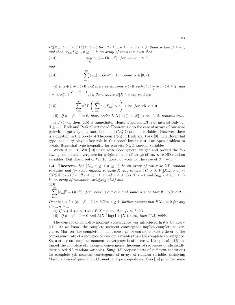
P (|Xni| > x) ≤ CP (|X| > x) for all i ≥ 1, n ≥ 1 and x ≥ 0. Suppose that β ≥ −1,and that ani, i ≥ 1, n ≥ 1 is an array of constants such that
(1.3) supi≥1|ani| = O(n−r) for some r > 0
and
(1.4)
∞∑
i=1
|ani| = O(nα) for some α ∈ [0, r).
(i) If α + β + 1 > 0 and there exists some δ > 0 such thatα
r+ 1 < δ ≤ 2, and
s = max(1 +α+ β + 1
r, δ), then, under E|X|s <∞, we have
(1.5)∞∑
n=1
nβP
(∣∣∣∣∣∞∑
i=1
aniXni
∣∣∣∣∣ > ε
)<∞ for all ε > 0.
(ii) If α+ β + 1 = 0, then, under E|X| log(1 + |X|) <∞, (1.5) remains true.
If β < −1, then (1.5) is immediate. Hence Theorem 1.3 is of interest only forβ ≥ −1. Baek and Park [9] extended Theorem 1.3 to the case of arrays of row-wisepairwise negatively quadrant dependent (NQD) random variables. However, thereis a question in the proofs of Theorem 1.3(i) in Baek and Park [9]. The Rosenthaltype inequality plays a key role in this proof, but it is still an open problem toobtain Rosenthal type inequality for pairwise NQD random variables.
When β > −1, Wu [10] dealt with more general weight and proved the fol-lowing complete convergence for weighted sums of arrays of row-wise ND randomvariables. But, the proof of Wu[10] does not work for the case of β = −1.
1.4. Theorem. Let Xni, i ≥ 1, n ≥ 1 be an array of row-wise ND randomvariables and for some random variable X and constant C > 0, P (|Xni| > x) ≤CP (|X| > x) for all i ≥ 1, n ≥ 1 and x ≥ 0. Let β > −1 and ani, i ≥ 1, n ≥ 1be an array of constants satisfying (1.3) and(1.6)∞∑
i=1
|ani|θ = O(nα) for some 0 < θ < 2 and some α such that θ + α/r < 2.
Denote s = θ+ (α+ β + 1)/r. When s ≥ 1, further assume that EXni = 0 for anyi ≥ 1, n ≥ 1.
(i) If α+ β + 1 > 0 and E|X|s <∞, then (1.5) holds.(ii) If α+ β + 1 = 0 and E|X|θ log(1 + |X|) <∞, then (1.5) holds.
The concept of complete moment convergence was introduced firstly by Chow[11]. As we know, the complete moment convergence implies complete conver-gence. Morover, the complete moment convergence can more exactly describe theconvergence rate of a sequence of random variables than the complete convergence.So, a study on complete moment convergence is of interest. Liang et al. [12] ob-tained the complete qth moment convergence theorems of sequences of identicallydistributed NA random variables. Sung [13] proposed sets of sufficient conditionsfor complete qth moment convergence of arrays of random variables satisfyingMarcinkiewicz-Zygmund and Rosenthal type inequalities. Guo [14] provided some
325

sufficient conditions for complete moment convergence of row-wise NA arrays ofrandom variables. Li and Zhang [15] established the complete moment conver-gence of moving average processes based on a sequence of identically distributedNA random variables as follows.
1.5. Theorem. Suppose that Yn =∑∞i=−∞ ai+nXi, n ≥ 1, where ai,−∞ < i <
∞ is a sequence of real numbers with∑∞−∞ |ai| < ∞ and Xi,−∞ < i < ∞
is a sequence of identically distributed and negatively associated random variableswith EX1 = 0, EX2
1 < ∞. Let 1/2 < r ≤ 1, p ≥ 1 + 1/(2r). Then E|X1|p < ∞implies that
∞∑
n=1
nrp−2−rl(n)E
(∣∣∣∣∣n∑
i=1
Yi
∣∣∣∣∣− εnr
)+
<∞ for all ε > 0.
The aim of this paper is to give a sufficient condition concerning completeqth moment convergence for arrays of row-wise END random variables. As anapplication, we not only generalize and extend the corresponding results of Baeket al. [8] and Wu [10] under some weaker conditions, but also greatly simplifytheir proof. Moreover, the complete qth moment convergence of moving averageprocesses based on a sequence of END random variables is also obtained, whichimproves the result of Li and Zhang [15]. The Baum-Katz type result for arraysof row-wise END random variables is also established.
Before we start our main results, we firstly state some definitions and lemmaswhich will be useful in the proofs of our main results. Throughout this paper, thesymbol C stands for a generic positive constant which may differ from one placeto another. The symbol I(A) denotes the indicator function of A. Let an bndenote that there exists a constant C > 0 such that an ≤ Cbn for all n ≥ 1. Denote(x)q+ = (max(x, 0))q, x+ = max(x, 0), x− = max(−x, 0), log x= ln max(e, x).
1.6. Definition. A sequence Xn, n ≥ 1 of random variables is said to bestochastically dominated by a random variable X if there exists a positive constantC, such that P (|Xn| > x) ≤ CP (|X| > x) for all x ≥ 0 and n ≥ 1.
The following lemma establish the fundamental inequalities for stochastic dom-ination, the proof is due to Wu [16].
1.7. Lemma. Let the sequence Xn, n ≥ 1 of random variables be stochasticallydominated by a random variable X. Then for any n ≥ 1, p > 0, x > 0, the followingtwo statements hold:
E|Xn|pI(|Xn| ≤ x) ≤ C (E|X|pI(|X| ≤ x) + xpP (|X| > x)) ,
E|Xn|pI(|Xn| > x) ≤ CE|X|pI(|X| > x).
The following lemma is the Hoffmann-Jφrgensen type inequality for sequencesof END random variables and is obtained by Shen [6].
1.8. Lemma. Let Xi, i ≥ 1 be a sequence of END random variables with EXi =0 and EX2
i < ∞ for every i ≥ 1 and set Bn =∑ni=1EX
2i for any n ≥ 1. Then
for all y > 0, t > 0, n ≥ 1,
P
(∣∣∣∣∣n∑
i=1
Xi
∣∣∣∣∣ ≥ y)≤ P
(max
1≤k≤n|Xk| > t
)+ 2M · exp
y
t− y
tlog
(1 +
yt
Bn
).
326

1.9. Definition. A real-valued function l(x), positive and measurable on [A,∞)
for some A > 0, is said to be slowly varying if limx→∞
l(xλ)
l(x)= 1 for each λ > 0.
1.10. Lemma. Let X be a random variable and l(x) > 0 be a slowly varyingfunction. Then
(i)∞∑
n=1
n−1E|X|αI(|X| > nγ) ≤ CE|X|α log(1 + |X|) for any α ≥ 0, γ > 0,
(ii)∞∑
n=1
nβl(n)E|X|αI(|X| > nγ) ≤ CE|X|α+(β+1)/γ l(|X|1/γ) for any β >
−1, α ≥ 0, γ > 0,
(iii)∞∑
n=1
nβl(n)E|X|αI(|X| ≤ nγ) ≤ CE|X|α+(β+1)/γ l(|X|1/γ) for any β <
−1, α ≥ 0, γ > 0.
Proof. We only prove (ii). Noting that β > −1, we have by Lemma 1.5 in Guo[14]that
∞∑
n=1
nβl(n)E|X|αI(|X| > nγ) =∞∑
n=1
nβl(n)∞∑
k=n
E|X|αI(kγ < |X| ≤ (k + 1)γ)
=
∞∑
k=1
E|X|αI(kγ < |X| ≤ (k + 1)γ)
k∑
n=1
nβl(n)
≤C∞∑
k=1
kβ+1l(k)E|X|αI(kγ < |X| ≤ (k + 1)γ) ≤ CE|X|α+(β+1)/γ l(|X|1/γ).
2. Main Results and the Proofs
In this section, let Xni, 1 ≤ i ≤ kn, n ≥ 1 be an array of row-wise END randomvariables with the same M in each row. Let kn, n ≥ 1 be a sequence of positiveintegers and an, n ≥ 1 be a sequence of positive constants. If kn = ∞ we willassume that the series
∑∞i=1Xni converges a.s. For any x ≥ 1, q > 0, set
X ′ni(x) = x1/qI(Xni > x1/q) +XniI(|Xni| ≤ x1/q)− x1/qI(Xni < −x1/q),
1 ≤ i ≤ kn, n ≥ 1. For any x ≥ 1, q > 0, it is clear that X ′ni(x), 1 ≤ i ≤ kn, n ≥ 1is an array of row-wise END random variables, since it is a sequence of monotonetransformations of Xni, 1 ≤ i ≤ kn, n ≥ 1.2.1. Theorem. Suppose that q > 0 and the following three conditions hold:
(i)∞∑
n=1
an
kn∑
i=1
E|Xni|qI(|Xni| > ε) <∞ for all ε > 0,
(ii) there exist 0 < r ≤ 2 and s > q/r such that
∞∑
n=1
an
(kn∑
i=1
E|Xni|r)s
<∞,
327

(iii) supx≥1
x−1/qkn∑
i=1
|EX ′ni(x)| → 0, as n→∞. Then for all ε > 0,
(2.1)∞∑
n=1
anE
(∣∣∣∣∣kn∑
i=1
Xni
∣∣∣∣∣− ε)q
+
<∞.
Proof. By Fubini’s theorem, we get that
∞∑
n=1
anE
(∣∣∣∣∣kn∑
i=1
Xni
∣∣∣∣∣− ε)q
+
=∞∑
n=1
an
∫ ∞
0
P
(∣∣∣∣∣kn∑
i=1
Xni
∣∣∣∣∣ > ε+ x1/q
)dx
≤∞∑
n=1
anP
(∣∣∣∣∣kn∑
i=1
Xni
∣∣∣∣∣ > ε
)+
∞∑
n=1
an
∫ ∞
1
P
(∣∣∣∣∣kn∑
i=1
Xni
∣∣∣∣∣ > x1/q
)dx =: I1 + I2.
We prove only I2 <∞, the proof of I1 <∞ is analogous. Using a simple integraland Fubini’s theorem, we obtain that for any q > 0 and a random variable X,
(2.2)
∫ ∞
1
P (|X| > x1/q)dx ≤ E|X|qI(|X| > 1).
Then by (2.2) and the subadditivity of probability measure we obtain the estimate
I2 ≤∞∑
n=1
an
∫ ∞
1
P
(∣∣∣∣∣kn∑
i=1
X ′ni(x)
∣∣∣∣∣ > x1/q
)dx+
∞∑
n=1
an
∫ ∞
1
kn∑
i=1
P(|Xni| > x1/q
)dx
≤∞∑
n=1
an
∫ ∞
1
P
(∣∣∣∣∣kn∑
i=1
X ′ni(x)
∣∣∣∣∣ > x1/q
)dx+
∞∑
n=1
an
kn∑
i=1
E|Xni|qI(|Xni| > 1)
=: I3 + I4.
By assumption (i), we have I4 <∞. By assumption (iii), we deduce that
(2.3) I3 ∞∑
n=1
an
∫ ∞
1
P
(∣∣∣∣∣kn∑
i=1
(X ′ni(x)− EX ′ni(x))
∣∣∣∣∣ > x1/q/2
)dx.
Set Bn =∑kni=1E(X ′ni(x) − EX ′ni(x))2, y = x1/q/2, t = x1/q/(2s), we have by
assumption (iii) and Lemma 1.8 that
(2.4)
P
(∣∣∣∣∣kn∑
i=1
(X ′ni(x)− EX ′ni(x))
∣∣∣∣∣ > x1/q/2
)
≤P(
max1≤i≤kn
|X ′ni(x)− EX ′ni(x)| > x1/q/(2s)
)+ 2Mes ·
(1 +
x2/q
4sBn
)−s
≤P(
max1≤i≤kn
|X ′ni(x)| > x1/q/(4s)
)+ 2Mes(4s)sx−2s/qBsn
≤kn∑
i=1
P(|X ′ni(x)| > x1/q/(4s)
)+ 2Mes(4s)sx−2s/q
(kn∑
i=1
E(X ′ni(x))2
)s
kn∑
i=1
P(|X ′ni(x)| > x1/q/(4s)
)+ x−2s/q
(kn∑
i=1
E(X ′ni(x))2
)s.
328

By (2.3) and (2.4), we obtain that
I3 ∞∑
n=1
an
∫ ∞
1
kn∑
i=1
P(|X ′ni(x)| > x1/q/(4s)
)dx(2.1)
+∞∑
n=1
an
∫ ∞
1
x−2s/q
(kn∑
i=1
E(X ′ni(x))2
)sdx
= I4 + I5.
Since |X ′ni(x)| ≤ |Xni|, we have P(|X ′ni(x)| > x1/q/(4s)
)≤ P
(|Xni| > x1/q/(4s)
).
By (2.2) and assumption (i), we conclude that
I4 ≤∞∑
n=1
an
∫ ∞
1
kn∑
i=1
P(|Xni| > x1/q/(4s)
)dx
≤∞∑
n=1
an
kn∑
i=1
(4s)qE|Xni|qI(|Xni| > 1/(4s)) <∞.
Hence, to complete the proof, it suffices to show that I5 <∞. From the definitionof X ′ni(x), since 0 < r ≤ 2, we have by Cr-inequality that(2.5)
E(X ′ni(x))2 EX2niI(|Xni| ≤ x1/q) + x2/qP (|Xni| > x1/q) ≤ 2x(2−r)/qE|Xni|r.
Noting that s > q/r, it is clear that
∫ ∞
1
x−sr/qdx < ∞. Then we have by (2.5)
and assumption (ii) that
I5 ∞∑
n=1
an
∫ ∞
1
x−2s/q
(kn∑
i=1
x(2−r)/qE|Xni|r)s
dx
≤∞∑
n=1
an
(kn∑
i=1
E|Xni|r)s ∫ ∞
1
x−sr/qdx∞∑
n=1
an
(kn∑
i=1
E|Xni|r)s
<∞.
Therefore, (2.1) holds.
2.2. Remark. Note that
∞∑
n=1
anE
(∣∣∣∣∣kn∑
i=1
Xni
∣∣∣∣∣− ε)q
+
=
∫ ∞
0
∞∑
n=1
anP
(∣∣∣∣∣kn∑
i=1
Xni
∣∣∣∣∣ > ε+ x1/q
)dx.
Thus, we obtain that the complete qth moment convergence implies the completeconvergence, i.e., (2.1) implies
∞∑
n=1
anP
(∣∣∣∣∣kn∑
i=1
Xni
∣∣∣∣∣ > ε
)<∞ for all ε > 0.
2.3. Theorem. Suppose that β > −1, p > 0, q > 0. Let Xni, i ≥ 1, n ≥ 1 bean array of row-wise END random variables which are stochastically dominated by
329

a random variable X. Let ani, i ≥ 1, n ≥ 1 be an array of constants satisfying(1.3) and
(2.6)∞∑
i=1
|ani|t n−1−β+r(p−t) for some 0 < t < p.
Furthermore, assume that
(2.7)
∞∑
i=1
a2ni n−µ for some µ > 0
if p ≥ 2. Assume further that EXni = 0 for all i ≥ 1 and n ≥ 1 when p ≥ 1. Then
(2.8)
E|X|q <∞, if q > p,
E|X|p log(1 + |X|) <∞, if q = p,
E|X|p <∞, if q < p,
implies
(2.9)
∞∑
n=1
nβE
(∣∣∣∣∣∞∑
i=1
aniXni
∣∣∣∣∣− ε)q
+
<∞ for all ε > 0.
Proof. We will apply Theorem 2.1 with an = nβ , kn =∞ and Xni, i ≥ 1, n ≥ 1replaced by aniXni, i ≥ 1, n ≥ 1. Without loss of generality, we can assumethat ani > 0 for all i ≥ 1, n ≥ 1(otherwise, we use a+
ni and a−ni instead of ani,respectively, and note that ani = a+
ni − a−ni). From (1.3) and (2.6), we can assumethat
(2.10) supi≥1|ani| ≤ n−r,
∞∑
i=1
|ani|t ≤ n−1−β+r(p−t).
Hence for any q ≥ t, we obtain by (2.10) that
(2.11)
∞∑
i=1
|ani|q =
∞∑
i=1
|ani|t|ani|q−t ≤ n−r(q−t)∞∑
i=1
|ani|t ≤ n−1−β+r(p−q).
330

For all ε > 0 , we have by (1.3), (2.8), (2.11), Lemma 1.7 and Lemma 1.10 that
(2.12)
∞∑
n=1
nβ∞∑
i=1
E|aniXni|qI(|aniXni| > ε)
∞∑
n=1
nβ∞∑
i=1
|ani|qE|X|qI(|X| > εnr)
≤∞∑
n=1
n−1+r(p−q)E|X|qI(|X| > εnr)
≤
∞∑
n=1
n−1+r(p−q)E|X|q, if q > p,
∞∑
n=1
n−1E|X|pI(|X| > εnr), if q = p,
∞∑
n=1
n−1+r(p−q), if q > p,
E|X|p log(1 + |X|), if q = p,
<∞.
When q < p, taking q′ such that max (q, t) < q′ < p, we have by (1.3), (2.8),(2.11), Lemma 1.7 and Lemma 1.10 that
(2.13)
∞∑
n=1
nβ∞∑
i=1
E|aniXni|qI(|aniXni| > ε)
≤εq−q′∞∑
n=1
nβ∞∑
i=1
E|aniXni|q′I(|aniXni| > ε)
∞∑
n=1
nβ∞∑
i=1
|ani|q′E|X|q′I(|X| > εnr)
≤∞∑
n=1
n−1+r(p−q′)E|X|q′I(|X| > εnr)
E|X|p <∞.
It is obvious that (2.8) implies E|X|p <∞. When p ≥ 2, It is clear that EX2 <∞.Noting that µ > 0, we can choose sufficiently large s such that β − µs < −1 ands > q/2. Then, by Lemma 1.7, (2.7) and EX2 <∞ we get that
(2.14)
∞∑
n=1
nβ
( ∞∑
i=1
Ea2niX
2ni
)s
∞∑
n=1
nβ
( ∞∑
i=1
a2ni
)s
∞∑
n=1
nβ−µs <∞.
331

When p < 2, since β > −1, we can choose sufficiently large s such that β+s(−1−β) < −1 and s > q/p, we have by (2.11), E|X|p <∞ and Lemma 1.7 that(2.15)
∞∑
n=1
nβ
( ∞∑
i=1
E|aniXni|p)s
∞∑
n=1
nβ
( ∞∑
i=1
|ani|p)s≤∞∑
n=1
nβ+s(−1−β) <∞.
When p < 1, combining (2.11), E|X|p < ∞ , β > −1, Cr-inequality and Lemma1.7, we obtain that
(2.16)
supx≥1
x−1/q∞∑
i=1
|EX ′ni(x)| ≤
∞∑
i=1
P (|aniXni| > 1) + supx≥1
x−1/q∞∑
i=1
E |aniXni| I(|aniXni| ≤ x1/q)
≤∞∑
i=1
P (|aniXni| > 1) + supx≥1
x−p/q∞∑
i=1
E |aniXi|p I(|aniXni| ≤ x1/q)
≤2
∞∑
i=1
E|aniXni|p ∞∑
i=1
|ani|p
≤n−1−β → 0, as n→∞.When p ≥ 1, since EXni = 0, we get that
EaniXniI(|aniXni| ≤ x1/q) = −EaniXniI(|aniXni| > x1/q).
Thus, we have by E|X|p <∞, β > −1, Cr-inequality and Lemma 1.7 that(2.17)
supx≥1
x−1/q∞∑
i=1
|EX ′ni(x)|
≤∞∑
i=1
P (|aniXni| > 1) + supx≥1
x−1/q∞∑
i=1
∣∣∣EaniXniI(|aniXni| > x1/q)∣∣∣
≤2∞∑
i=1
E|aniXni|I(|aniXni| > 1)∞∑
i=1
|ani|pE|X|pI(|X| > nr)∞∑
i=1
|ani|p
≤n−1−β → 0, as n→∞.Thus, by (2.12)–(2.17), we see that assumptions (i), (ii) and (iii) in Theorem 2.1are fulfilled. Therefore (2.9) holds by Theorem 2.1.
2.4. Remark. When 1+α+β > 0, the conditions (1.3), (2.6) and (2.7) are weakerthan the conditions (1.3) and (1.6). In fact, taking t = θ, p = θ + (1 + α + β)/r,we immediately get (2.6) by (1.6). Noting that θ < 2, we obtain by (1.3) and (1.6)that
∞∑
i=1
a2ni ≤ sup
i≥1|ani|2−θ
∞∑
i=1
|ani|θ n−(r(2−θ)−α).
Since θ < 2 − α/r, we have µ =: r(2 − θ) − α > 0. Therefore (2.7) holds. So,Theorem 2.3 not only extends the result of Wu [10] for ND random variables to
332

END case, but also obtains the weaker sufficient condition of complete qth momentconvergence of weighted sums for arrays of row-wise END random variables. Itis worthy to point out that the method used in this article is novel, which differsfrom that of Wu [10]. Our method greatly simplify the proof of Wu [10].
Note that conditions (1.3) and (2.6) together imply
(2.18)
∞∑
i=1
|ani|p n−1−β .
From the proof of Theorem 2.3, we can easily see that if q > 0 of Theorem 2.3 isreplaced by q ≥ p, then condition (2.6) can be replaced by the weaker condition(2.18).
2.5. Theorem. Suppose that β > −1, p > 0. Let Xni, i ≥ 1, n ≥ 1 be anarray of row-wise END random variables which are stochastically dominated by arandom variable X. Let ani, i ≥ 1, n ≥ 1 be an array of constants satisfying(1.3) and (2.18). Furthermore, assume that (2.7) holds if p ≥ 2. Assume furtherthat EXni = 0 for all i ≥ 1 and n ≥ 1 when p ≥ 1. Then
(2.19)
E|X|q <∞, if q > p,
E|X|p log(1 + |X|) <∞, if q = p,
implies that (2.9) holds.
2.6. Remark. As in Remark 2.4 , when 1 +α+β = 0, the conditions (1.3), (2.7)and (2.18) are weaker than the conditions (1.3) and (1.6).
Take q < p in Theorem 2.3 and q = p in Theorem 2.5, by Remark 2.2 we canimmediately obtain the following corollary:
2.7. Corollary. Suppose that β > −1, p > 0. Let Xni, i ≥ 1, n ≥ 1 be anarray of row-wise END random variables which are stochastically dominated by arandom variable X. Assume further that EXni = 0 for all i ≥ 1 and n ≥ 1 whenp ≥ 1. Let ani, i ≥ 1, n ≥ 1 be an array of constants satisfying (1.3), (2.7) and
(2.20)∞∑
i=1
|ani|t n−1−β+r(p−t) for some 0 < t ≤ p.
(i) If t < p, then E|X|p <∞ implies (1.5).(ii) If t = p, then E|X|p log(1 + |X|) <∞ implies (1.5).
The following corollary establish complete qth moment convergence for movingaverage processes under a sequence of END non-identically distributed randomvariables, which extends the corresponding results of Li and Zhang [15] to the caseof sequences of END non-identically distributed random variables. Moreover, ourresult covers the case of r > 1, which was not considered by Li and Zhang [15].
2.8. Corollary. Suppose that Yn =∑∞i=−∞ ai+nXi, n ≥ 1, where ai,−∞ < i <
∞ is a sequence of real numbers with∑∞−∞ |ai| < ∞ and Xi,−∞ < i < ∞
is a sequence of END random variables with mean zero which are stochastically
333

dominated by a random variable X. Let r > 1/2, p ≥ 1 + 1/(2r), q > 0. Then
(2.21)
E|X|q <∞, if q > p,
E|X|p log(1 + |X|) <∞, if q = p,
E|X|p <∞, if q < p,
implies that
(2.22)∞∑
n=1
nrp−2E
(∣∣∣∣∣n−r
n∑
i=1
Yi
∣∣∣∣∣− ε)q
+
<∞, for all ε > 0.
Proof. Note that
n−rn∑
i=1
Yi =∞∑
i=−∞
n−r
n∑
j=1
ai+j
Xi.
We will apply Theorem 2.3 with β = rp − 2, t = 1, ani = n−r∑nj=1 ai+j and
Xni, i ≥ 1, n ≥ 1 replaced by Xi,−∞ < i < ∞. Noting that∑∞−∞ |ai| < ∞,
r > 1/2 and p ≥ 1 + 1/(2r), we can easily see that the conditions (1.3) and (1.6)hold for θ = 1, α = 1 − r. Therefore (2.22) holds by (2.21), Theorem 2.3 andRemark 2.2.
Similar to the proof of Corollary 2.8, we can get the following Baum-Katz typeresult for arrays of row-wise END random variables as follows.
2.9. Corollary. Let Xni, 1 ≤ i ≤ n, n ≥ 1 be an array of row-wise ENDrandom variables which are stochastically dominated by a random variable X. Letr > 1/2, p > 1, q > 0. Assume further that EXni = 0 for all i ≥ 1 and n ≥ 1when p ≥ r. Then
E|X|q <∞, if q > p/r,
E|X|p/r log(1 + |X|) <∞, if q = p/r,
E|X|p/r <∞, if q < p/r,
implies that
∞∑
n=1
np−2−rqE
(∣∣∣∣∣n∑
i=1
Xni
∣∣∣∣∣− εnr
)q
+
<∞, for all ε > 0.
References
[1] Hsu, P. L. and Robbins, H. Complete convergence and the law of large numbers. Proc. Natl.
Acad. Sci. U.S.A., 33(2), 25–31, 1947.
[2] Baum, L. E. and Katz, M. Convergence rates in the law of large numbers. Trans. Am.Math. Soc., 120(1), 108–123, 1965.
[3] Liu, L. Precise large deviations for dependent random variables with heavy tails. Statist.
Probab. Lett., 79(9), 1290–1298, 2009.[4] Lehmann, E. L. Some concepts of dependence. Ann. Math. Statist., 37(5), 1137–1153,
1966.
[5] Joag-Dev, K. and Proschan, F. Negative association of random variables with applications.Ann. Statist., 11(1), 286–295, 1983.
334
[6] Shen, A. T. Probability inequalities for END sequence and their applications. J. Inequal.
Appl., 2011, 98, 2011.
[7] Chen, Y. Q. and Chen, A. Y. and Ng, K. W. The strong law of large numbers for extendnegatively dependent random variables. J. Appl. Prob., 47(4), 908–922, 2010.
[8] Baek, J. I., Choi, I. B. and Niu, S. l. On the complete convergence of weighted sums for
arrays of negatively associated variables. J. Korean Stat. Soc., 37(1), 73–80, 2008.[9] Baek, J. I. and Park, S. T. Convergence of weighted sums for arrays of negatively dependent
random variables and its applications. J. Stat. Plan. Infer., 140(9), 2461–2469, 2010.
[10] Wu, Q. A complete convergence theorem for weighted sums of arrays of rowwise negativelydependent random variables. J. Inequal. Appl.,2012: 50, 2012.
[11] Chow, Y. S. On the rate of moment convergence of sample sums and extremes. Bull. Inst.
Math. Acad. Sinica, 16(3), 177–201, 1988.[12] Liang, H. Y., Li, D. L. and Rosalsky, A. Complete moment convergence for sums of neg-
atively associated random variables. Acta Math. Sinica, English Series, 26(3), 419–432,2010.
[13] Sung, S. H. Complete qth moment convergence for arrays of random variables. J. Inequal.
Appl., 2013, 24, 2013.[14] Guo, M. L. On complete moment convergence of weighted sums for arrays of row-wise
negatively associated random variables. Stochastics: Int. J. Probab. Stoch. Proc., 86(3),
415-428, 2014.[15] Li, Y. X. and Zhang, L. X. Complete moment convergence of moving-average processes
under dependence assumptions. Statist. Probab. Lett., 70(3), 191–197, 2004.
[16] Wu, Q. Y. Probability Limit Theory for Mixed Sequence. China Science Press, Beijing, 2006.
335


Hacettepe Journal of Mathematics and StatisticsVolume 43 (2) (2014), 337 – 346
A new calibration estimator in stratified doublesampling
Nursel Koyuncu a ∗ and Cem Kadılar a †
Abstract
In the present article, we consider a new calibration estimator of thepopulation mean in the stratified double sampling. We get more effi-cient calibration estimator using new calibration weights compared tothe straight estimator. In addition, the estimators derived are ana-lyzed for different populations by a simulation study. The simulationstudy shows that new calibration estimator is highly efficient than theexisting estimator.
Keywords: Calibration, Auxiliary information, Stratified double sampling.
2000 AMS Classification: 62D05
1. Introduction
When the auxiliary information is available, the calibration estimator is widelyused in the sampling literature to improve the estimates. Many authors, such asDeville and Sarndal [2], Estevao and Sarndal [3], Arnab and Singh [1], Farrell andSingh [4], Kim et al.[5], Kim and Park [6], Koyuncu and Kadilar etc.[8], definedsome calibration estimators using different constraints. In the stratified randomsampling, calibration approach is used to get optimum strata weights. Tracy etal.[9] defined calibration estimators in the stratified random sampling and stratifieddouble sampling. In this study, we try to improve the calibration estimator in thestratified double sampling.
aHacettepe University, Department of Statistics, Beytepe, 06800, Ankara, Turkey.∗Email: [email protected]†Email: [email protected]

N. Koyuncu and C. Kadılar
2. Notations
Consider a finite population of N units consists of L strata such that the hth
stratum consists of Nh units andL∑h=1
Nh = N . From the hth stratum of Nh units,
draw a preliminary large sample of mh units by the simple random samplingwithout replacement (SRSWOR) and measure the auxiliary character,xhi, only.Select a sub-sample of nh units from the given preliminary large sample of mh
units by SRSWOR and measure both the study variable, yhi and auxiliary variable,
xhi. Let x∗h = 1mh
mh∑i=1
xhi and s∗2hx = 1mh−1
mh∑i=1
(xhi − x∗h)2 denote the first phase
sample mean and variance, respectively. Besides, assume that xh = 1nh
nh∑i=1
xhi
, s2hx = 1
nh−1
nh∑i=1
(xhi − xh)2 and yh = 1nh
nh∑i=1
yhi , s2hy = 1
nh−1
nh∑i=1
(yhi − yh)2
denote the second phase sample means and variances for the auxiliary and studycharacters, respectively.
Calibration estimator, defined by Tracy et al.[9], is given by
(2.1) yst(d) =
L∑
h=1
W ∗hyh,
where W ∗h are calibration weights minimizing the chi-square distance measure
(2.2)L∑
h=1
(W ∗h −Wh)2
QhWh
subject to calibration constraints defined by
(2.3)L∑
h=1
W ∗hxh =L∑
h=1
Whx∗h,
(2.4)
L∑
h=1
W ∗hs2hx =
L∑
h=1
Whs∗2hx.
The Lagrange function using calibration constraints and chi-square distancemeasure is given by
(2.5)
4 =L∑
h=1
(W ∗h −Wh)2
QhWh−2λ1(
L∑
h=1
W ∗hxh−L∑
h=1
Whx∗h)−2λ2(
L∑
h=1
W ∗hs2hx−
L∑
h=1
Whs∗2hx),
where λ1 and λ2 are Lagrange multipliers. Setting the derivative of ∆ withrespect to W ∗h equals to zero gives
338

(2.6) W ∗h = Wh +QhWh(λ1xh + λ2s2hx).
Substituting (2.6) in (2.3) and (2.4) respectively, we get
(L∑
h=1
QhWhx2h
) (L∑
h=1
QhWhxhs2hx
)
(L∑
h=1
QhWhxhs2hx
) (L∑
h=1
QhWhs4hx
)
[ λ1
λ2
]=
L∑h=1
Whx∗h−
L∑h=1
Whxh
L∑h=1
Whs∗2hx−
L∑h=1
Whs2hx
Solving the system of equations for lambdas, we obtain
λ1 =
(L∑h=1
QhWhs4hx)(
L∑h=1
Whx∗h −
L∑h=1
Whxh)− (L∑h=1
Whs∗2hx −
L∑h=1
Whs2hx)(
L∑h=1
QhWhxhs2hx)
(L∑h=1
QhWhs4hx)(
L∑h=1
QhWhx2h)− (
L∑h=1
QhWhxhs2hx)2
,
λ2 =
(L∑h=1
Whs∗2hx −
L∑h=1
Whs2hx)(
L∑h=1
QhWhx2h)− (
L∑h=1
QhWhxhs2hx)(
L∑h=1
Whx∗h −
L∑h=1
Whxh)
(L∑h=1
QhWhs4hx)(
L∑h=1
QhWhx2h)− (
L∑h=1
QhWhxhs2hx)2
.
Substituting these values into (2.6), we get the weights as given by
W ∗h = Wh+
(QhWhxh)[(L∑h=1
QhWhs4hx)(
L∑h=1
Wh(x∗h − xh))− (L∑h=1
Wh(s∗2hx − s2hx))(
L∑h=1
QhWhxhs2hx)]
(L∑h=1
QhWhs4hx)(
L∑h=1
QhWhx2h)− (
L∑h=1
QhWhxhs2hx)2
+
(QhWhs2hx)[(
L∑h=1
Wh(s∗2hx − s2hx))(
L∑h=1
QhWhx2h)− (
L∑h=1
QhWhxhs2hx)(
L∑h=1
Wh(x∗h − xh))]
(L∑h=1
QhWhs4hx)(
L∑h=1
QhWhx2h)− (
L∑h=1
QhWhxhs2hx)2
Writing these weights in (2.1), we get the calibration estimator as
yst(d) = (
L∑
h=1
Whyh) + β1(d)(
L∑
h=1
Wh(x∗h− xh)) + β2(d)(
L∑
h=1
Wh(s∗2hx− s2hx)),
where betas are given by
β1(d) =
(L∑h=1
QhWhs4hx)(
L∑h=1
QhWhxhyh)− (L∑h=1
QhWhxhs2hx)(
L∑h=1
QhWhyhs2hx)
(L∑h=1
QhWhs4hx)(
L∑h=1
QhWhx2h)− (
L∑h=1
QhWhxhs2hx)2
,
339

N. Koyuncu and C. Kadılar
β2(d) =
(L∑h=1
QhWhx2h)(
L∑h=1
QhWhyhs2hx)− (
L∑h=1
QhWhxhs2hx)(
L∑h=1
QhWhxhyh)
(L∑h=1
QhWhs4hx)(
L∑h=1
QhWhx2h)− (
L∑h=1
QhWhxhs2hx)2
.
3. Suggested Estimator
Motivated by Tracy et al.[9], we consider a new calibration estimator as
(3.1) yst(dnew) =L∑
h=1
Ωhyh.
Using the chi-square distance
(3.2)L∑
h=1
(Ωh −Wh)2
QhWh,
and subject to calibration constraints defined by Koyuncu[7]
(3.3)L∑
h=1
Ωhxh =L∑
h=1
Whx∗h,
(3.4)L∑
h=1
Ωhs2hx =
L∑
h=1
Whs∗2hx,
(3.5)
L∑
h=1
Ωh =
L∑
h=1
Wh,
we can write the Lagrange function given by
4 =L∑
h=1
(Ωh −Wh)2
QhWh− 2λ1(
L∑
h=1
Ωhxh −L∑
h=1
Whx∗h)− 2λ2(
L∑
h=1
Ωhs2hx −
L∑
h=1
Whs∗2hx)
− 2λ3(L∑
h=1
Ωh −L∑
h=1
Wh),
Setting ∂44Ωh
= 0, we obtain
(3.6) Ωh = Wh +QhWh(λ1xh + λ2s2hx + λ3).
Substituting (3.6) in (3.3)-(3.5), respectively, we get the following system ofequations
340

(L∑
h=1
QhWhx2h
) (L∑
h=1
QhWhxhs2hx
) (L∑
h=1
QhWhxh
)
(L∑
h=1
QhWhxhs2hx
) (L∑
h=1
QhWhs4hx
) (L∑
h=1
QhWhs2hx
)
(L∑
h=1
QhWhxh
) (L∑
h=1
QhWhs2hx
) (L∑
h=1
QhWh
)
[λ1
λ2
λ3
]=
L∑h=1
Whx∗h−
L∑h=1
Whxh
L∑h=1
Whs∗2hx−
L∑h=1
Whs2hx
0
Solving the system of equations for lambdas, we obtain
λ1 =A
D,λ2 =
B
D,λ3 =
C
D,
where
A =
(L∑
h=1
Wh(x∗h − xh)
)[( L∑
h=1
QhWh
)( L∑
h=1
QhWhs4hx
)−( L∑
h=1
QhWhs2hx
)2]
+
(L∑
h=1
Wh(s∗2hx − s2hx)
)[( L∑
h=1
QhWhxh
)( L∑
h=1
QhWhs2hx
)
−( L∑
h=1
QhWh
)( L∑
h=1
QhWhs2hxxh
)]
B =
(L∑
h=1
Wh(s∗2hx − s2hx)
)[( L∑
h=1
QhWh
)( L∑
h=1
QhWhx2h
)−( L∑
h=1
QhWhxh
)2]
−( L∑
h=1
Wh(x∗h − xh))[( L∑
h=1
QhWhs2hxxh
)( L∑
h=1
QhWh
)
−( L∑
h=1
QhWhxh
)( L∑
h=1
QhWhs2hx
)]
C =( L∑
h=1
Wh(x∗h − xh))[( L∑
h=1
QhWhs2hx
)( L∑
h=1
QhWhs2hxxh
)−( L∑
h=1
QhWhxh
)( L∑
h=1
QhWhs4hx
)]
+( L∑
h=1
Wh(s∗2hx − s2hx))[( L∑
h=1
QhWhxh
)( L∑
h=1
QhWhxhs2hx
)
−( L∑
h=1
QhWhx2h
)( L∑
h=1
QhWhs2hx
)]
341

N. Koyuncu and C. Kadılar
D =( L∑
h=1
QhWh
)( L∑
h=1
QhWhs4hx
)( L∑
h=1
QhWhx2h
)−( L∑
h=1
QhWhxh
)2( L∑
h=1
QhWhs4hx
)
−( L∑
h=1
QhWh
)( L∑
h=1
QhWhs2hxxh
)2
−( L∑
h=1
QhWhs2hx
)2( L∑
h=1
QhWhx2h
)
+ 2( L∑
h=1
QhWhxh
)( L∑
h=1
QhWhs2hx
)( L∑
h=1
QhWhxhs2hx
)
Substituting these lambdas in (3.6) and then (3.1), we get
yst(dnew) = yst+β1(dnew)(L∑
h=1
Wh(x∗h−xh))+β2(dnew)(L∑
h=1
Wh(s∗2hx−s2hx)),
where β1(dnew) = A∗
D and β2(dnew) = B∗
D
A∗ =
(L∑
h=1
QhWhxhyh
)[( L∑
h=1
QhWh
)( L∑
h=1
QhWhs4hx
)−( L∑
h=1
QhWhs2hx
)2]
−(
L∑
h=1
QhWhs2hxyh
)[( L∑
h=1
QhWhs2hxxh
)( L∑
h=1
QhWh
)−( L∑
h=1
QhWhxh
)( L∑
h=1
QhWhs2hx
)]
+
(L∑
h=1
QhWhyh
)[( L∑
h=1
QhWhs2hx
)( L∑
h=1
QhWhs2hxxh
)−( L∑
h=1
QhWhxh
)( L∑
h=1
QhWhs4hx
)]
B∗ =
(L∑
h=1
QhWhxhyh
)[( L∑
h=1
QhWhxh
)( L∑
h=1
QhWhs2hx
)−( L∑
h=1
QhWh
)( L∑
h=1
QhWhs2hxxh
)]
+
(L∑
h=1
QhWhs2hxyh
)[( L∑
h=1
QhWh
)( L∑
h=1
QhWhx2h
)−( L∑
h=1
QhWhxh
)2]
+
(L∑
h=1
QhWhyh
)[( L∑
h=1
QhWhxh
)( L∑
h=1
QhWhxhs2hx
)−( L∑
h=1
QhWhx2h
)( L∑
h=1
QhWhs2hx
)]
4. Theoretical Variance
We can write the estimators yst(d) and yst(dnew) as follows:
(4.1) yst(α) =L∑
h=1
Whyh + β1(α)
L∑
h=1
Wh(xh − x∗h) + β2(α)
L∑
h=1
Wh(s2hx − s∗2hx)
where α = d, dnew. To find the variance of estimators, let us define followingequations:
342
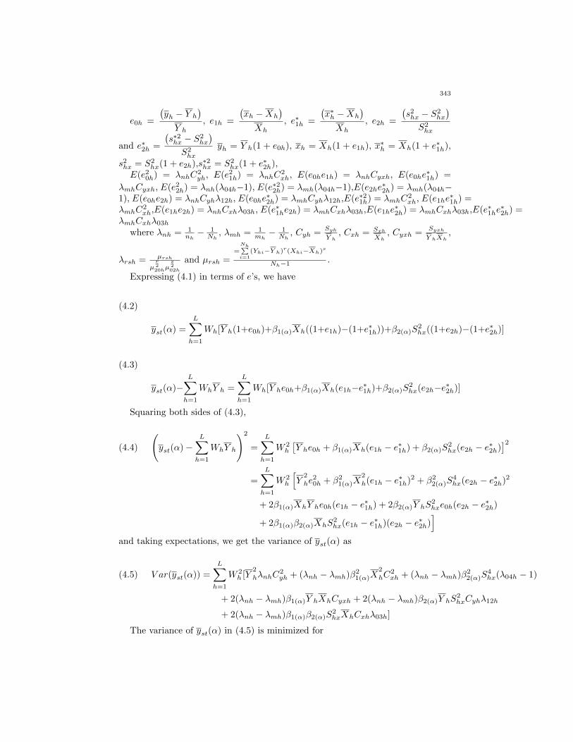
e0h =
(yh − Y h
)
Y h, e1h =
(xh −Xh
)
Xh
, e∗1h =
(x∗h −Xh
)
Xh
, e2h =
(s2hx − S2
hx
)
S2hx
and e∗2h =
(s∗2hx − S2
hx
)
S2hx
yh = Y h(1 + e0h), xh = Xh(1 + e1h), x∗h = Xh(1 + e∗1h),
s2hx = S2
hx(1 + e2h),s∗2hx = S2hx(1 + e∗2h),
E(e20h) = λnhC
2yh, E(e2
1h) = λnhC2xh, E(e0he1h) = λnhCyxh, E(e0he
∗1h) =
λmhCyxh, E(e22h) = λnh(λ04h−1), E(e∗22h) = λmh(λ04h−1),E(e2he
∗2h) = λmh(λ04h−
1), E(e0he2h) = λnhCyhλ12h, E(e0he∗2h) = λmhCyhλ12h,E(e∗21h) = λmhC
2xh, E(e1he
∗1h) =
λmhC2xh,E(e1he2h) = λnhCxhλ03h, E(e∗1he2h) = λmhCxhλ03h,E(e1he
∗2h) = λmhCxhλ03h,E(e∗1he
∗2h) =
λmhCxhλ03h
where λnh = 1nh− 1
Nh, λmh = 1
mh− 1
Nh, Cyh =
Syh
Y h, Cxh = Sxh
Xh, Cyxh =
Syxh
Y hXh,
λrsh = µrsh
µr220hµ
s202h
and µrsh ==
Nh∑i=1
(Yhi−Y h)r(Xhi−Xh)s
Nh−1 .
Expressing (4.1) in terms of e’s, we have
(4.2)
yst(α) =L∑
h=1
Wh[Y h(1+e0h)+β1(α)Xh((1+e1h)−(1+e∗1h))+β2(α)S2hx((1+e2h)−(1+e∗2h)]
(4.3)
yst(α)−L∑
h=1
WhY h =L∑
h=1
Wh[Y he0h+β1(α)Xh(e1h−e∗1h)+β2(α)S2hx(e2h−e∗2h)]
Squaring both sides of (4.3),
(yst(α)−
L∑
h=1
WhY h
)2
=
L∑
h=1
W 2h
[Y he0h + β1(α)Xh(e1h − e∗1h) + β2(α)S
2hx(e2h − e∗2h)
]2(4.4)
=L∑
h=1
W 2h
[Y
2
he20h + β2
1(α)X2
h(e1h − e∗1h)2 + β22(α)S
4hx(e2h − e∗2h)2
+ 2β1(α)XhY he0h(e1h − e∗1h) + 2β2(α)Y hS2hxe0h(e2h − e∗2h)
+ 2β1(α)β2(α)XhS2hx(e1h − e∗1h)(e2h − e∗2h)
]
and taking expectations, we get the variance of yst(α) as
V ar(yst(α)) =L∑
h=1
W 2h [Y
2
hλnhC2yh + (λnh − λmh)β2
1(α)X2
hC2xh + (λnh − λmh)β2
2(α)S4hx(λ04h − 1)(4.5)
+ 2(λnh − λmh)β1(α)Y hXhCyxh + 2(λnh − λmh)β2(α)Y hS2hxCyhλ12h
+ 2(λnh − λmh)β1(α)β2(α)S2hxXhCxhλ03h]
The variance of yst(α) in (4.5) is minimized for
343
N. Koyuncu and C. Kadılar
V ar(yst(α))
∂β1(α)= 0,
(4.6) β1(α) =−β2(α)S
2hxCxhλ03h − Y hCyxhXhC2
xh
,
V ar(yst(α))
∂β2(α)= 0,
(4.7) β2(α) =−β1(α)XhCxhλ03h − Y hCyhλ12h
S2hx(λ04h − 1)
,
Substituting (4.6) in (4.7) or vice versa, we have optimum betas as given by
β1(α) =SyhSxh
λ12hλ03h − λ11h(λ04h − 1)
(λ04h − 1)− λ203h
, β2(α) =SyhS2xh
λ11hλ03h − λ12h
(λ04h − 1)− λ203h
The resulting (minimum) variance of yst(α) is given by
V ar(yst(α))(4.8)
=L∑
h=1
W 2hY
2
h
[λnhC
2yh − (λnh − λmh)
C2yxh(λ04h − 1) + C2
xhC2yhλ
212h − 2CyxhCyhCxhλ03hλ12h
C2xh[(λ04h − 1)− λ2
03h]
]
=L∑
h=1
W 2hY
2
hC2yh
[λmh + (λnh − λmh)
[1− λ2
11h −(λ12h − λ11hλ03h)2
(λ04h − 1)− λ203h
]]
5. Simulation Study
To study the properties of the proposed calibration estimator, we perform asimulation study by generating four different artificial populations where x∗hi andy∗hi values are from different distributions given in Table 1. To get different levelof correlations between study and auxiliary variables, we apply some transforma-tions given in Table 2. Each population consists of three strata having 500 units.After selecting a preliminary sample of size 300 from each stratum, we select 5000times for the second sample whose sample of sizes are 30 and 50. The correlationcoefficients between study and auxiliary variables for each stratum are taken asρxy1 = 0.5 ,ρxy2 = 0.7 and ρxy3 = 0.9 . The quantities,S1x = 4.5 , S2x = 6.2 ,S3x = 8.4 and S1y = S2y = S3y are taken as fixed in each stratum as in Tracy et al.[9]. We calculate the empirical mean square error and percent relative efficiency,respectively, using following formulas:
344
MSE(yst(α)) =
N
n
∑k=1
[yst(α)− Y ]2
(Nn
) , α = d, dnew
PRE =MSE(yst(d))
MSE(yst(dnew))∗ 100
From Table 3, the simulation study shows that new calibration estimator isquite efficient than the existing estimator.
6. Conclusion
In this study we derived new calibration weights in stratified double sampling.The performance of the weights are compared with a simulation study. We foundthat suggested weights perform better than existing weights.
References
[1] Arnab, R. and Singh, S. A note on variance estimation for the generalized regression pre-dictor, Australian and New Zealand Journal of Statistics 47 (2), 231–234, 2005.
[2] Deville, J. C. and Sarndal, C. E. Calibration estimators in survey sampling, Journal of the
American Statistical Association 87, 376–382, 1992.[3] Estevao, V. M. and Sarndal, C. E. A functional form approach to calibration, Journal of
Official Statistics 16, 379–399, 2000.[4] Farrell, P. J. and Singh, S. Model-assisted higher order calibration of estimators of variance,
Australian and New Zealand Journal of Statistics 47 (3), 375–383, 2005.
[5] Kim, J. M., Sungur, E. A. and Heo T. Y. Calibration approach estimators in stratified sam-pling, Statistics and Probability Letters 77 (1), 99–103, 2007.
[6] Kim, J. K. and Park, M. Calibration estimation in survey sampling, International Statistical
Review78 (1), 21–29, 2010.[7] Koyuncu, N. Application of calibration method to estimators in sampling theory,(PhD. The-
sis, Hacettepe University Department of Statistics, 2012).
[8] Koyuncu, N. and Kadilar, C. Calibration estimator using different distance measures instratified random sampling, International Journal of Modern Engineering Research 3 (1),
415–419, 2013.
[9] Tracy, D. S., Singh, S. and Arnab, R. Note on calibration in stratified and double sampling,Survey Methodology 29, 99–104, 2003.
345

N. Koyuncu and C. Kadılar
Table 1. Parameters and Distributions of Study and Auxiliary Variables
Parameters and distributionsof study variable
Parameters and distributionsof auxiliary variable
I. Population, h=1,2,3
f(y∗hi) = 1Γ(1.5)
y∗1.5−1hi e−y
∗hi f(x∗hi) = 1
Γ(0.3)x∗0.3−1hi e−x
∗hi
II. Population, h=1,2,3
f(y∗hi) = 1√2πe−
y∗2hi2 f(x∗hi) = 1
Γ(0.3)x∗0.3−1hi e−x
∗hi
Table 2. Properties of Strata
Strata Study Variable Auxiliary Variable
1. Stratum y1i = 50 + y∗1i x1i = 15 +√
(1 − ρ2xy1)x∗1i + ρxy1
S1xS1y
y∗1i
2. Stratum y2i = 150 + y∗2i x2i = 100 +√
(1 − ρ2xy2)x∗2i + ρxy2
S2xS2y
y∗2i
3. Stratum y3i = 50 + y∗3i x3i = 200 +√
(1 − ρ2xy3)x∗3i + ρxy3
S3xS3y
y∗3i
Table 3. Empirical Mean Square Error (MSE) and Percent RelativeEfficiency (PRE) of Estimators
Population Empirical MSE(yst(d)) Empirical MSE(yst(dnew)) PRE
I (mh = 30) 61205495678 65730798 93115.4
I (mh = 50) 626914412 38472456 1629.515
II (mh = 30) 6.8404e+11 50343013 1358759
II (mh = 50) 245901177 35046173 701.6491
346

Hacettepe Journal of Mathematics and StatisticsVolume 43 (2) (2014), 347 – 360
Bayesian estimation of Marshall–Olkin extendedexponential parameters under various
approximation techniques
Sanjay Kumar Singh a ∗, Umesh Singh a, and Abhimanyu Singh Yadav a
Abstract
In this paper, we propse Bayes estimators of the parameters ofMarshall Olkin extended exponential distribution (MOEED) intro-duced by Marshall-Olkin [2] for complete sample under squarederror loss function (SELF). We have used different approximationtechniques to obtain the Bayes estimate of the parameters. AMonte Carlo simulation study is carried out to compare the per-formance of proposed estimators with the corresponding maximumlikelihood estimator (MLE’s) on the basis of their simulated risk.A real data set has been considered for illustrative purpose of the study.
Keywords: Bayes estimator, Squared error loss function, Lindley’s approxima-tion method, T-K approximation, MCMC method.
2000 AMS Classification: 62F15, 62C10
1. Introduction
Due to simple, elegant and closed form of distribution function, Exponential dis-tribution is most popular distribution for life time data analysis. Further Borlowand Proschan [22] have discussed the justification regarding the use of exponen-tial distribution as the failure law of complex equipment. However its uses arerestricted to constant hazard rate, which is difficult to justify in many real situ-ations. Thus one can think to develop alternative model which has non-constanthazard rate. In the literature, various methods may be used to generalise exponen-tial distributions and these generalized models have the property of non-constanthazard rate like Weibull, gamma and exponentiated exponential distribution etc.These generalized models are frequently used to analyse the life time data. Inaddition Marshall and Olkin [2] introduced a method of adding a new parameterto a specified distribution. The resulting distribution is known as Marshall Olkinextended distribution. The general methodology regarding the introducing a new
aDepartment of Statistics and DST-CIMS, Banaras Hindu University, Varanasi-221005∗Corresponding author e–mail: [email protected]
S. K. Singh et al.
parameters is as follows:Let F (x) be the survival function of existing or specified distribution then, thesurvival function of new distribution can be obtained by using following relation
S(x) =αF (x)
1− αF (x); −∞ < x <∞, α > 0
where α = 1−α and S(x) is the survival function of new distribution. Note that,when α = 1, S(x) = F (x). Thus, the form of density corresponding to the survivalfunction S(x) is obtained as,
f(x, α) =αf(x)
1− αF (x)
2
Further more, Marshall and Olkin derived a distribution by introducing the sur-vival function of exponential distribution say (F (x) = e−λx). The resulting distri-bution is known as Marshall Olkin extended exponential distribution (MOEED)with increasing and decreasing failure rate functions see [2]. The probability den-sity function (pdf) and cumulative distribution function (cdf) of this distributionare given as:
(1.1) f(x, α, λ) =αλe−λx
(1− αe−λx)2; x, α, λ ≥ 0
(1.2) F (x, α, λ) =1− e−λx
1− αe−λx ; x, α, λ ≥ 0
respectively. The considered distribution is very useful in life testing problem andit may be used as a good alternative to the gamma, Weibull and other exponen-tiated family of distributions. The basic properties related to this distributionhave been discussed in [2]. The density function (1) has increasing failure rate forα ≥ 1 , decreasing failure rate for α ≤ 1 and constant failure rate for α = 1 similarto one parameter exponential distribution. G. Srinivasa Rao et al [3] used thisdistribution for making reliability test plan with sampling point of view. Shapeof this distribution is presented bellow see figure 1. for different choices of shapeand scale parameter.
In this paper, we mainly consider both the informative and non-informativepriors under squared error loss function to compute the Bayes estimators of pa-rameters. It has been noticed that the Bayes estimators of the parameters cannotbe expressed in a nice closed form. Thus the different numerical approximationprocedures are used to obtain Bayes estimator. Here we use the Lindley’s, Tier-ney and Kadane (T-K) approximation methods and Markov Chain Monte Carlo(MCMC) technique to compute the Bayes estimators of the parameters.
The rest of the paper is organized as follows: In section 2.1, we describe theclassical estimation with maximum likelihood estimator (MLE) of parameters. Insection 2.2, we compute Bayes estimator of parameters with gamma prior and insection 2.2.1, 2.2.2 and 2.2.3 we describe different Bayesian approaches like Lind-ley Approximation, Tierney and Kadane approximation and Monte Carlo Markov
348
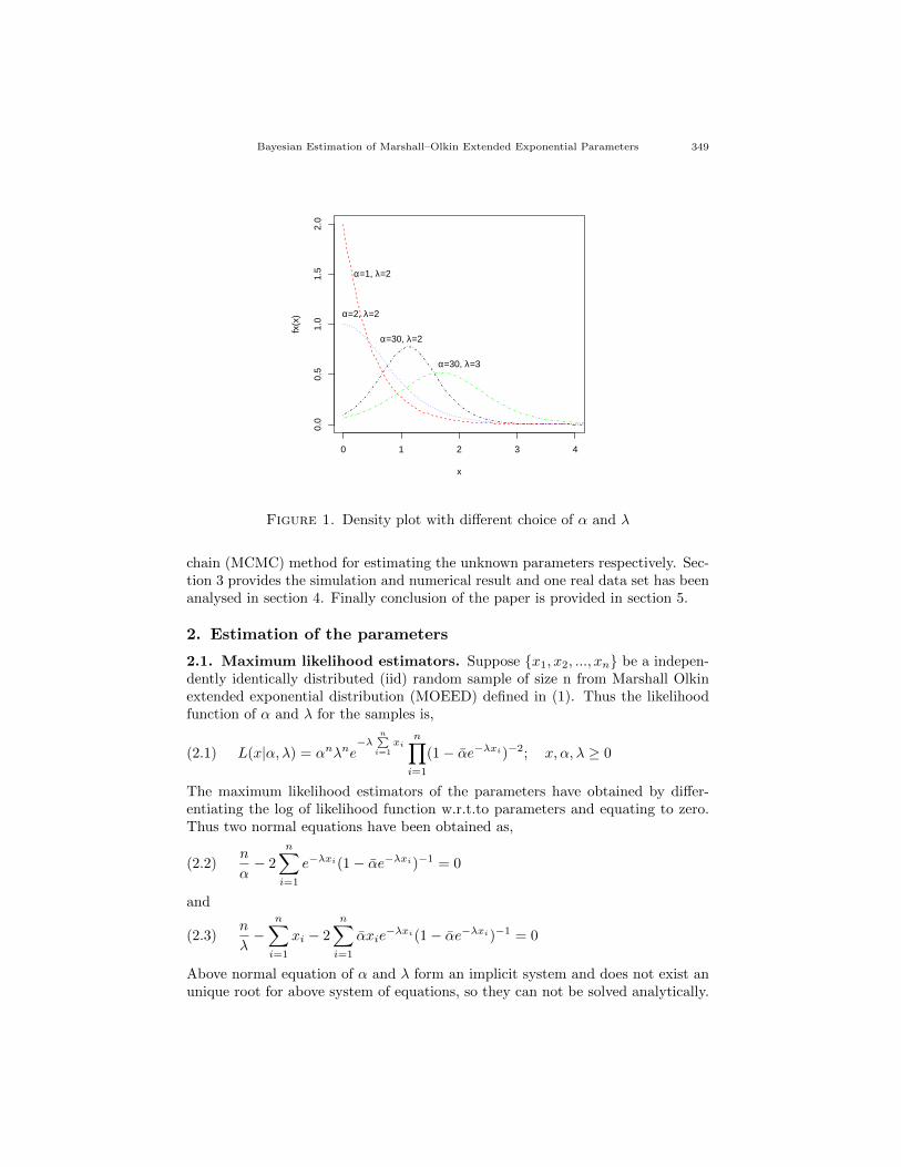
Bayesian Estimation of Marshall–Olkin Extended Exponential Parameters
0 1 2 3 4
0.0
0.5
1.0
1.5
2.0
x
fx(x
)
α=1, λ=2
α=2, λ=2
α=30, λ=2
α=30, λ=3
Figure 1. Density plot with different choice of α and λ
chain (MCMC) method for estimating the unknown parameters respectively. Sec-tion 3 provides the simulation and numerical result and one real data set has beenanalysed in section 4. Finally conclusion of the paper is provided in section 5.
2. Estimation of the parameters
2.1. Maximum likelihood estimators. Suppose x1, x2, ..., xn be a indepen-dently identically distributed (iid) random sample of size n from Marshall Olkinextended exponential distribution (MOEED) defined in (1). Thus the likelihoodfunction of α and λ for the samples is,
(2.1) L(x|α, λ) = αnλne−λ
n∑i=1
xin∏
i=1
(1− αe−λxi)−2; x, α, λ ≥ 0
The maximum likelihood estimators of the parameters have obtained by differ-entiating the log of likelihood function w.r.t.to parameters and equating to zero.Thus two normal equations have been obtained as,
(2.2)n
α− 2
n∑
i=1
e−λxi(1− αe−λxi)−1 = 0
and
(2.3)n
λ−
n∑
i=1
xi − 2
n∑
i=1
αxie−λxi(1− αe−λxi)−1 = 0
Above normal equation of α and λ form an implicit system and does not exist anunique root for above system of equations, so they can not be solved analytically.
349
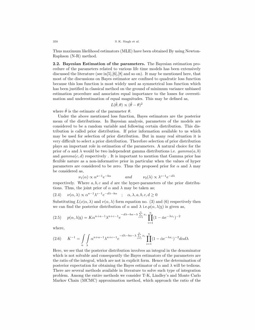
S. K. Singh et al.
Thus maximum likelihood estimators (MLE) have been obtained By using Newton-Raphson (N-R) method.
2.2. Bayesian Estimation of the parameters. The Bayesian estimation pro-cedure of the parameters related to various life time models has been extensivelydiscussed the literature (see in[5],[6],[8] and so on). It may be mentioned here, thatmost of the discussions on Bayes estimator are confined to quadratic loss functionbecause this loss function is most widely used as symmetrical loss function whichhas been justified in classical method on the ground of minimum variance unbiasedestimation procedure and associates equal importance to the losses for overesti-mation and underestimation of equal magnitudes. This may be defined as,
L(θ, θ) ∝ (θ − θ)2
where θ is the estimate of the parameter θ.Under the above mentioned loss function, Bayes estimators are the posterior
mean of the distributions. In Bayesian analysis, parameters of the models areconsidered to be a random variable and following certain distribution. This dis-tribution is called prior distribution. If prior information available to us whichmay be used for selection of prior distribution. But in many real situation it isvery difficult to select a prior distribution. Therefore selection of prior distributionplays an important role in estimation of the parameters. A natural choice for theprior of α and λ would be two independent gamma distributions i.e. gamma(a, b)and gamma(c, d) respectively . It is important to mention that Gamma prior hasflexible nature as a non-informative prior in particular when the values of hyperparameters are considered to be zero. Thus the proposed prior for α and λ maybe considered as,
ν1(α) ∝ αa−1e−bα and ν2(λ) ∝ λc−1e−dλ
respectively. Where a, b, c and d are the hyper-parameters of the prior distribu-tions. Thus, the joint prior of α and λ may be taken as;
(2.4) ν(α, λ) ∝ αa−1λc−1e−dλ−bα ; α, λ, a, b, c, d ≥ 0
Substituting L(x|α, λ) and ν(α, λ) form equation no. (3) and (6) respectively thenwe can find the posterior distribution of α and λ i.e.p(α, λ|x) is given as,
(2.5) p(α, λ|x) = Kαn+a−1λn+c−1e−dλ−bα−λ
n∑i=1
xin∏
i=1
(1− αe−λxi)−2
where,
(2.6) K−1 =
∫
α
∫
λ
αn+a−1λn+c−1e−dλ−bα−λ
n∑i=1
xin∏
i=1
(1− αe−λxi)−2dαdλ
Here, we see that the posterior distribution involves an integral in the denominatorwhich is not solvable and consequently the Bayes estimators of the parameters arethe ratio of the integral, which are not in explicit form. Hence the determination ofposterior expectation for obtaining the Bayes estimator of α and λ will be tedious.There are several methods available in literature to solve such type of integrationproblem. Among the entire methods we consider T-K, Lindley’s and Monte CarloMarkov Chain (MCMC) approximation method, which approach the ratio of the
350

Bayesian Estimation of Marshall–Olkin Extended Exponential Parameters
integrals as a whole and produce a single numerical result. These methods aredescribed bellow:
2.2.1. Bayes estimator using Lindley’s Approximation. We consider the Lindley’sapproximation method to obtain the Bayes estimates of the parameters, whichincludes the posterior expectation is expressible in the form of ratio of integral asfollow:
(2.7) I(x) = E(α, λ|x) =
∫u(α, λ)eL(α,λ)+G(α,λ)d(α, λ)∫
eL(α,λ)+G(α,λ)d(α, λ)
where,u(α, λ)= is a function of α and λ onlyL(α, λ)= Log- likelihood functionG(α, λ)= Log of joint prior densityAccording to D. V. Lindley [1], if ML estimates of the parameters are availableand n is sufficiently large then the above ratio of the integral can be approximatedas:
I(x) = u(α, λ) + 0.5[(uλλ + 2uλτλ)σλλ + (uαλ + 2uατλ)σαλ + (uλα + 2uλτα)σλα +
(uαα + 2uατα)σαα] +1
2[(uλσλλ + uασλα)(Lλλλσλλ + Lλαλσλα + Lαλλσαλ +
Lααλσαα) + (uλσαλ + uασαα)(Lαλλσλλ + Lλαασλα + Lαλασαλ + Lααασαα)]
where α and λ is the MLE of α and λ respectively, and
uα =∂u(α, λ)
∂α, uλ =
∂u(α, λ)
∂λ, uαλ =
∂u(α, λ)
∂α∂λ, uλα =
∂u(α, λ)
∂λ∂α, uαα =
∂2u(α, λ)
∂α2,
uλλ =∂2u(α, λ)
∂λ2, Lαα =
∂2L(α, λ)
∂α2, Lλλ =
∂2L(α, λ)
∂λ2, Lααα =
∂3L(α, λ)
∂α3,
Lααλ =∂3L(α, λ)
∂α∂α∂λ, Lλλα =
∂3L(α, λ)
∂λ∂λ∂α, Lλαλ =
∂3L(α, λ)
∂λ∂α∂λ, Lααλ =
∂3L(α, λ)
∂α∂α∂λ,
Lαλλ =∂3L(α, λ)
∂α∂λ∂λ, Lλαα =
∂3L(α, λ)
∂λ∂α∂α, pα =
∂G(α, λ)
∂α, pλ =
∂G(α, λ)
∂λ
After substitution of p(α, λ|x) from (7) in above equation (9) then this integralmust be reduces like Lindley’s integral, where:
u(α, λ) = α
L(α, λ) = n lnα+ n lnλ− λn∑
i=1
xi − 2
n∑
i=1
ln(1− αe−λxi) and
G(α, λ) = (a− 1) lnα+ (c− 1) lnλ− (bα+ dλ)
it may verified that,
uα = 1, uαα = uλλ = uαλ = uλα = 0, pα =a− 1
α− b, pλ =
c− 1
λ− d
Lα =n
α− 2
n∑i=1
e−λxi
(1− αe−λxi) , Lαα =−nα2
+ 2n∑i=1
e−2λxi
(1− αe−λxi)2 ,
Lααα =2n
α3− 4
n∑i=1
e−3λxi
(1− αe−λxi)3 , Lλ =n
λ−
n∑i=1
xi − 2n∑i=1
xiαe−λxi
(1− αe−λxi) ,
351

S. K. Singh et al.
Lλλ =−nλ2
+ 2n∑i=1
x2i αe−λxi
(1− αe−λxi) + 2n∑i=1
x2i α
2e−2λxi
(1− αe−λxi)2 ,
Lλλλ =2n
λ3− 2
n∑i=1
x3i αe−λxi
(1− αe−λxi) − 6n∑i=1
x3i α
2e−2λxi
(1− αe−λxi)2 − 4n∑i=1
x3i α
3e−3λxi
(1− αe−λxi)3 ,
Lααλ = Lλαα = −4n∑i=1
xie−2λxi
(1− αe−λxi)2 − 4n∑i=1
xiαe−3λxi
(1− αe−λxi)3 ,
Lαλλ = Lλλα = −2n∑i=1
x2i e−λxi
(1− αe−λxi) − 6n∑i=1
x2i αe−2λxi
(1− αe−λxi)2 − 4n∑i=1
x2i α
2e−3λxi
(1− αe−λxi)3
If α and λ are orthogonal then σij = 0 for i 6= j and σij =(− 1
Lij
)for i = j After
evaluation of all U-terms, L-terms, and p- terms at the point (α, λ) and using theabove expression, the approximate Bayes estimator of α under SELF is,
(2.8) αLS = α+ uαpασαα + 0.5(uασαασλλLαλλ + uασ
2ααLααα
)
and similarly the Bayes estimate for λ under SELF is,uλ = 1, uαα = uλλ = uαλ = uλα = 0 and remaining L-terms and -terms will besame as above thus we have,
(2.9) λLS = λ+ uλpλσλλ + 0.5(uλσ
2λλLλλλ + uλσαασλλLααλ
)
2.2.2. Bayes estimators using Tierney and Kadane’s (T-K) Approximation. Lind-ley’s method of solving integral is accurate enough but one of the problems of thismethod is that it requires evaluation of third order partial derivatives and in
p-parameters case the total number of derivatives isp(p+ 1)(p+ 2)
6then this ap-
proximation will be quite complicated. thus one can think about T-K approxima-tion method and this method may be used as an alternative to Lindley’s method.According to the Tierney and Kadane’s approximation any ratio of the integral ofthe form,
(2.10) u(α, λ) = Ep(α,λ|x)[u(α, λ|x)] =
∫α,λ
enL∗(α,λ)d(α, λ)
∫α,λ
enL0(α,λ)d(α, λ)
where,
(2.11) L0(α, λ) =1
n[L(α, λ) + ln ν(α, λ)] and L∗(α, λ) = L0(α, λ) +
1
nlnu(α, λ)
Thus estimate can be obtained as,
(2.12) u(α, λ) =
√|Σ∗||Σ0|
e[nL∗(α∗,λ∗)−L0(α0,λ0)]
where (α∗, λ∗) and (α0, λ0) maximize L∗(α, λ) and L0(α, λ) respectively, and Σ∗and Σ0 are the negative of the inverse of the matrices of second derivatives ofL∗(α, λ) and L0(α, λ) at the point (α∗, λ∗) and (α0, λ0) respectively. In our study,based on (14) the function L0(α, λ) is given as,
(2.13)
352

Bayesian Estimation of Marshall–Olkin Extended Exponential Parameters
L0(α, λ) =1
n[(n+a−1) lnα−bα+(n+c−1) lnλ−λ(d+
n∑
i=1
xi)−2n∑
i=1
ln(1−αe−λxi)]
and thus for the Bayes estimator of α and λ under SELF using this approximation(17) can be written as,
(2.14) αT−KS (α, λ) =
√|Σ∗||Σ0|
e[nLα∗ (α∗,λ∗)−L0(α0,λ0)]
(2.15) λT−KS (α, λ) =
√|Σ∗||Σ0|
e[nLλ∗ (α∗,λ∗)−L0(α0,λ0)]
where
Lα∗ (α, λ) = Lα0 (α, λ) +1
nlnα and Lλ∗(α, λ) = Lλ0 (α, λ) +
1
nlnλ
2.2.3. Bayes estimator using Monte Carlo Markov Chain (MCMC) method. Inthis section, we propose Monte Carlo Markov Chain (MCMC) method for ob-taining the Bayes estimates of the parameters. Thus we consider the MCMCtechnique namely Gibbs sampler and Metropolis-Hastings algorithm to generatesample from the posterior distribution and then compute the Bayes estimate. TheGibbs sampler is best applied on problems where the marginal distributions of theparameters of interest are difficult to calculate, but the conditional distributions ofeach parameter given all the other parameters and the data have nice forms. If theconditional distributions of the parameters have standard forms, then they can besimulated easily. But generating samples from full conditionals corresponding tojoint posterior is not easily manageable. Therefore we considered the Metropolis-Hastings algorithm. Metropolis step is used to extract samples from some of thefull conditional to complete a cycle in Gibbs chain . For more detail about MCMCmethod see for example Gelfand and Smith [23], Upadhya and Gupta [24] . Thusutilizing the concept of Gibbs sampling procedure as mentioned above, generatessample from the posterior density function (7) under the assumption that parame-ters α and λ have independent Gamma density function with hyper parameters a,b and c, d respectively. To incorporate this technique we consider full conditionalposterior densities of α and λ are written as ,
(2.16) π(α|λ, x) ∝ αn+a−1e−bαn∏
i=1
(1− αe−λxi)−2
(2.17) π(λ|α, x) ∝ λn+c−1e−λ(d+
n∑i=1
xi)n∏
i=1
(1− αe−λxi)−2
The Gibbs algorithm consist the following steps
• Start with k=1 and initial values (α0, λ0)• Using M-H algorithm generate posterior sample for α and λ from (18) and
(19) respectively, where asymptotic normal distribution of full conditionaldensities are considered as the proposal.• Repeat step 2, for all k = 1, 2, 3, . . . ,M and obtain (α1, λ1), (α2, λ2), ...(αM , λM )• After obtaining the posterior sample the Bayes estimates of α and λ with
respect to the SELF are as follows:
353
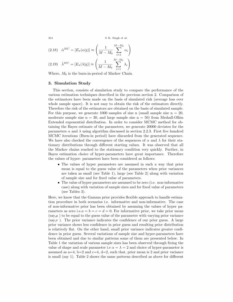
S. K. Singh et al.
(2.18) αMC = [Eπ(α|x)] ≈(
1
M −M0
M−M0∑
i=1
αi
)
(2.19) λMC = [Eπ(λ|x)] ≈(
1
M −M0
M−M0∑
i=1
λi
)
Where, M0 is the burn-in-period of Markov Chain.
3. Simulation Study
This section, consists of simulation study to compare the performance of thevarious estimation techniques described in the previous section 2. Comparison ofthe estimators have been made on the basis of simulated risk (average loss overwhole sample space). It is not easy to obtain the risk of the estimators directly.Therefore the risk of the estimators are obtained on the basis of simulated sample.For this purpose, we generate 1000 samples of size n (small sample size n = 20,moderate sample size n = 30, and large sample size n = 50) from Mrshall-OlkinExtended exponential distribution. In order to consider MCMC method for ob-taining the Bayes estimate of the parameters, we generate 20000 deviates for theparameters α and λ using algorithm discussed in section 2.2.3. First five hundredMCMC iterations (Burn-in period) have discarded from the generated sequence.We have also checked the convergence of the sequences of α and λ for their sta-tionary distributions through different starting values. It was observed that allthe Markov chains reached to the stationary condition very quickly. Further, inBayes estimation choice of hyper-parameters have great importance. Thereforethe values of hyper- parameters have been considered as follows:
• The values of hyper parameters are assumed in such a way that priormean is equal to the guess value of the parameters when prior variancesare taken as small (see Table 1), large (see Table 2) along with variationof sample size and for fixed value of parameters.• The value of hyper parameters are assumed to be zero (i.e. non-informative
case) along with variation of sample sizes and for fixed value of parameters(see Tables 3).
Here, we know that the Gamma prior provides flexible approach to handle estima-tion procedure in both scenarios i.e. informative and non-informative. The caseof non-informative prior has been obtained by assuming the values of hyper pa-rameters as zero i.e.a = b = c = d = 0. For informative prior, we take prior mean(say,µ ) to be equal to the guess value of the parameter with varying prior variance(say,ν ). The prior variance indicates the confidence of our prior guess. A largeprior variance shows less confidence in prior guess and resulting prior distributionis relatively flat. On the other hand, small prior variance indicates greater confi-dence in prior guess. Several variations of sample size and hyper-parameters havebeen obtained and due to similar patterns some of them are presented below. InTable 1 the variation of various sample sizes has been observed through fixing thevalue of shape and scale parameter i.e α = λ = 2 and choice of hyper-parameter isassumed as a=4, b=2 and c=4, d=2, such that, prior mean is 2 and prior varianceis small (say 1). Table 2 shows the same patterns described as above for different
354

Bayesian Estimation of Marshall–Olkin Extended Exponential Parameters
choice of hyper-parameters which is assumed as a=0.4, b=0.2 and c=0.4, d=0.2,such that prior mean is 2 but prior variance is very large (say 10). Table 3 exhibitssimilar results under consideration of non-informative prior scenario. It is also ob-served that the risks of all the estimators decrease as sample size increases in allthe considered cases. As we expected, it is also observed that when we considerinformative prior, the proposed Bayes estimators behave better than the classicalmaximum likelihood estimators. But in case of non-informative prior, their be-haviour are almost same as MLE, which may be seen in the following connectedtables (see Table 1,2 and 3).
4. Real Illustration
In this section; we analyze a real data set from A. Wood [21] to illustrate ourestimation procedure. The data is based on the failure times of the release ofsoftware given in terms of hours with average life time be 1000 hours from thestarting of the execution of the software. This data can be regarded as an orderedsample of size 16 are given as,
0.519 0.968 1.430 1.893 2.490 3.058 3.625 4.4425.218 5.823 6.539 7.083 7.485 7.846 8.205 8.564
Given data set have been already considered by Rao et al.[3] to construct a sam-pling plan only if the life time has Marshall-Olkin extended exponential distribu-tion. To identify the validity of proposed model criterion of log-likelihood, Akaikeinformation criterion (AIC) and Bayesian information criterion (BIC) have beendiscussed. It has been verified that the given data set provides better fit than otherexponetiated family such as exponential, Generalized exponential and gamma dis-tributions see Table (5) and empirical cumulative distribution function (ECDF)plot of this data is represented in figure (2).To calculate the Bayes estimates of the parameters in absence of prior informa-tion, we consider the non-informative prior. Further we calculate the Maximumlikelihood estimates of the parameter and also Bayes estimates of the parametersunder different considered estimation methods which are presented in Table 4. TheMCMC iterations of α and λ are plotted respectively. Density and Trace plots areindicating that the MCMC samples are well mixed and stationary achieved seefigure 3.
5. Conclusion
In this paper, we have considered the classical as well as Bayesian estimation ofthe unknown parameters of the Marshall- Olkin extended exponential distributionunder various approximation techniques. On the basis of extensive study we mayconclude the followings:
• Under informative setup the performance of Bayes estimators of the pa-rameters is better than the maximum likelihood estimators (MLE’s) inall considered approximation techniques and also Lindley’s approximationtechnique works quite well than rest of other methods such as T-K andMCMC.
355

S. K. Singh et al.
• Under non-informative set up, we observed that T-K approximation methodbehaves like maximum likelihood estimators (MLE’s) and performs wellthan Lindleys and MCMC approximation methods.
References
[1] Lindley, D.V. Approximate Bayes method, Trabajos de estadistica, Vol. 31, 223–237, 1980.
[2] Marshall A.W. and Olkin, I. A new method for adding a parameter to a family of distri-
butions with application to the exponential and Weibull families, Biometrika 84, 641–652,1997.
[3] Rao, G. S., Ghitany M.E., and Kantam, R.R. L. Reliability test plans for Marshall-Olkinextended exponential distribution, Applied Mathematical Science, Vol. 3, no. 55, 2745–2755,
2009.
[4] Gupta R.D. and Kundu, D. Generalized exponential distribution: Existing result and somerecent developement, J.Stat. Plan. Inf., 137, pp. 3537–3547, 2007.
[5] Singh, R., Singh, S.K., Singh, U., and Singh, G.P. Bayes estimator of the generalized-
exponential parameters under Linex loss function using Lindley’s Approximation, DataScience Journal, Vol. 7, 2008.
[6] Singh, P.K., Singh, S.K., and Singh, U. Bayes estimator of the Inverse Gaussian Parame-
ters under GELF using Lindley’s Approximation, Communications in Statistics-Simulationand computation, 37, 1750–1762, 2008.
[7] Panahi, Haniyeh and Asadi, Saeid Analysis of the type II hybrid censored Burr type XII
distribution under Linex loss function, Applied Mathematical Science, Vol. 5, no. 79, 3929–3942, 2011.
[8] Preda, V., Panaitescu, E., and Constantinescu, A. Bayes estimators of Modified–WeibullDistribution parameters using Lindley’s approximation, Wseas Transactions on Mathemat-
ics: issue, Vol. 9, 2010.
[9] Chen, M. and Shao, Q. Monte Carlo estimation of Bayesian credible and HPD intervals, J.Comput. Graph. Statist., 8, 189–193, 1999.
[10] Karandikar, R. L. On the Markov Chain Monte Carlo (MCMC) method, Sadhana, Vol. 31,
Part2, pp. 81–104, April 2006.[11] Kadane, J. B. and Lazar, N.A. Method and criteria for model selection, Journal of the
American Statistical Association, Vol. 99, pp. 279–290, 2004.
[12] Berger, J.O. and Sun, D. Bayesian analysis for the Poly-Weibull distribution, Journal ofthe American Statistical Association, Vol. 88, 1412–1418, 1993.
[13] Jaeckel, L.A. Robust estimates of location; symmetry and asymmetry contamination, Ann.
Math. Statist., Vol. 42, pp. 1020–1034, Jun 1971.[14] Miller, R.B. Bayesian analysis of the two-parameter gamma distribution, Technometrics,
Vol. 22, 65–69, 1980.
[15] Lawless, J. F. Statistical Models and Methods for Lifetime data, (Wiley, New York, 1982).[16] Gupta, R.D. and Kundu, D. Exponentiated exponential distribution: an alternative to
gamma and Weibull distributions, Biometrical J., 43 (1), 117–130, 2001.[17] Gupta, R.D. and Kundu, D. Generalized exponential distributions: diDerent methods of
estimations, J. Statist. Comput. Simulations, 69 (4), 315–338, 2001.
[18] Gupta, R.D. and Kundu, D. Generalized exponential distributions; Statistical Infer- ences,Journal of Statistical Theory and Applications, 2002 1, 101–118, 2002.
[19] Birnbaum, Z.W. and Saunders, S. C. Estimation for a family of life distributions with ap-
plications to fatigue. Journal of Applied Probability, 6, 328–347, 1969.[20] Zheng, G. On the Fisher information matrix in type-II censored data from the exponentiated
exponential family, Biometrical Journal, 44 (3), 353–357, 2002.
[21] Wood, A. Predicting software reliability, IEEE Transactions on Software Engineering, 22,69–77, 1996.
[22] Barlow, R. E. and Proschan, F. Statistical theory of reliability and life testing probability
models, (Holt, Rinehart and Winston, New York, 1975).
356

Bayesian Estimation of Marshall–Olkin Extended Exponential Parameters
[23] Gelfand, A. E. and Smith, A. F.M. Sampling-Based Approaches to Calculating Marginal
Densities, Journal of the American Statistical Association, Vol. 85, No. 410. pp. 398–409,
1990.[24] Upadhyay, S.K. and Gupta, A. A Bayes Analysis of Modified Weibull Distribution via
Markov Chain, Monte Carlo Simulation. Journal. of Statistical Computation and Simulation,
80 (3), 241–254, 2010.
Table 1. This table represents the estimates of the parametersobtained through various estimation techniques when prior meanis 2 and prior variance is 1 i.e.µ = 2,ν = 1 and also the quantity insecond row exhibits the average expected loss over sample spacei.e. risks of corresponding estimators.
Size MLE T-K Lindley’s MCMC
n αM λM αT−KS λT−KS αLS λLS αMCS λMC
S
202.23773 2.06460 2.23737 2.06445 1.77297 1.98913 2.28136 2.077941.39995 0.39985 1.40010 0.39962 0.26508 0.26972 1.15025 0.30349
302.21472 2.04999 2.21469 2.04986 1.95451 2.00332 2.23035 2.050501.19207 0.26914 1.19255 0.26902 0.24508 0.21117 0.96397 0.19768
502.26295 2.06143 2.26278 2.06138 2.11909 2.03343 2.25792 2.053261.00657 0.19669 1.00657 0.19668 0.39802 0.16998 0.88427 0.16388
Table 2. This table represents the estimates of the parametersobtained through various estimation techniques when prior meanis 2 and prior variance is 10 i.e.µ = 2,ν = 10 and also the quantityin second row exhibits the average expected loss over sample spacei.e. risks of corresponding estimators.
Size MLE T-K Lindley’s MCMC
n αM λM αT−KS λT−KS αLS λLS αMCS λMC
S
202.23773 2.06460 2.23834 2.06459 2.28362 2.00365 2.18074 2.008271.39995 0.39985 1.40243 0.40017 1.32136 0.36720 1.40399 0.42792
302.21472 2.04999 2.21525 2.05007 2.24926 2.00974 2.14724 1.990701.19207 0.26914 1.19239 0.26918 1.14257 0.25448 1.18310 0.28731
502.26295 2.06143 2.26265 2.06135 2.28564 2.03720 2.21927 2.027271.00657 0.19669 1.00658 0.19668 0.98506 0.18914 0.99635 0.20304
357

S. K. Singh et al.
Table 3. Table represents the estimates of the parameters ob-tained through various estimation techniques and also the quan-tity in square bracketed exhibits the average expected loss oversample space i.e. risks under non-informative prior.
Size MLE T-K Lindley’s MCMC
n αM λM αT−KS λT−KS αLS λLS αMCS λMC
S
202.23773 2.06460 2.23750 2.06448 2.34036 2.00526 2.15852 1.985381.39995 0.39985 1.40114 0.40005 1.60352 0.37905 1.46574 0.47475
302.21472 2.04999 2.21514 2.05005 2.28201 2.01046 2.12848 1.972251.19207 0.26914 1.19233 0.26916 1.30748 0.25955 1.23519 0.32177
502.26295 2.06143 2.26262 2.06137 2.30415 2.03762 2.21263 2.022071.00657 0.19669 1.00659 0.19669 1.07019 0.19134 1.01519 0.21145
Table 4. This table represents the estimates of the parametersobtained by various methods of estimation for real data set underthe assumption that prior information assume to be non-informative.
Size MLE T-K Lindley’s MCMC
n αM λM αT−KS λT−KS αLS λLS αMCS λMC
S
16 8.62532 0.50074 8.62534 0.50074 9.12253 0.48963 8.62581 0.49910
Table 5. This Table represents the values of Log-likelihood, AICand BIC for different models in real data set.
Distribution -log LInformation CriterionAIC BIC
Exponential 40.762 83.524 84.296Generalized Exponential 38.836 81.673 83.218
Gamma 38.629 81.258 82.803MOEED 38.044 80.089 81.634
358

Bayesian Estimation of Marshall–Olkin Extended Exponential Parameters
2 4 6 8
0.2
0.4
0.6
0.8
1.0
x
Cum
ulat
ive
Dis
trib
utio
n F
unct
ion
Empirical CDFCDF for MLECDF for Bayes
Figure 2. CDF plot for considered real data set
359

S. K. Singh et al.
8.3 8.4 8.5 8.6 8.7 8.8 8.9
01
23
4
Density plot of α
N = 19501 Bandwidth = 0.01075
Den
sity
0.3 0.4 0.5 0.6 0.7
01
23
45
67
Density plot of λ
N = 19501 Bandwidth = 0.007076
Den
sity
Trace plot of α
Time
0 5000 10000 15000 20000
8.3
8.5
8.7
8.9
Trace plot of λ
Time
0 5000 10000 15000 20000
0.3
0.4
0.5
0.6
0.7
Figure 3. Posterior density and trace plot for considered realdata set.
360

Hacettepe Journal ofADVICE TO AUTHORS
Mathematics and Statistics
Hacettepe Journal of Mathematics and Statistics publishes short to medium lengthresearch papers and occasional survey articles written in English. All papers arerefereed to international standards.
Address for Correspondence
Editorial Office,Hacettepe Journal of Mathematics and Statistics,Hacettepe University,Faculty of Science,Department of Mathematics,06532 Beytepe,Ankara,Turkey.
E-mail: [email protected]: Editors: + 90 312 297 7859
+ 90 312 297 7898
Associate Editor: + 90 312 297 7880
Fax : + 90 312 299 2017
Web Page : http//www.hjms.hacettepe.edu.tr
Advise to Authors : The style of articles should be lucid but concise. Thetext should be preceded by a short descriptive title and an informative abstract ofnot more than 100 words. Keywords or phrases and the 2010 AMS Classificationshould also be included.The main body of the text should be divided into num-bered sections with appropriate headings. Items should be numbered in the form2.4. Lemma, 2.5. Definition. These items should be referred to in the text usingthe form Lemma 2.4., Definition 2.5. Figures and tables should be incorporatedin the text. A numbered caption should be placed above them. References shouldbe punctuated according to the following examples, be listed in alphabetical or-der according to in the (first) author’ s surname, be numbered consecutively andreferred to in the text by the same number enclosed in square brackets. Onlyrecognized abbreviations of the names of journals should be used.
[1 ] Banaschewski, B. Extensions of topological spaces, Canad. Math. Bull.7 (1), 1–22, 1964.
[2 ] Ehrig, H. and Herrlich, H. The construct PRO of projection spaces: itsinternal structure, in: Categorical methods in Computer Science, LectureNotes in Computer Science 393 (Springer-Verlag, Berlin, 1989), 286–293.
[3 ] Hurvich, C. M. and Tsai, C. L. Regression and time series model selectionin small samples, Biometrika 76 (2), 297–307, 1989.
[4 ] Papoulis, A. Probability random variables and stochastic process (McGraw-Hill, 1965).

Hacettepe Journal ofINSTRUCTIONS FOR AUTHORS
Mathematics and Statistics
Preparation of Manuscripts : Manuscripts will be typeset using the LATEXtypesetting system. Authors should prepare the article using the HJMS stylebefore submission by e-mail. The style bundle contains the styles for the article andthe bibliography as well as example of formatted document as pdf file. The authorsshould send their paper directly to [email protected] with the suggestionof area editor and potential reviewers for their submission. The editorial officemay not use these suggestions, but this may help to speed up the selection ofappropriate reviewers.
Copyright : No manuscript should be submitted which has previously been pub-lished, or which has been simultaneously submitted for publication elsewhere. Thecopyright in a published article rests solely with the Faculty of Science of HacettepeUniversity, and the paper may not be reproduced in whole in part by any meanswhatsoever without prior written permission.
Notice : The content of a paper published in this Journal is the sole responsibilityof the author or authors, and its publication does not imply the concurrence ofthe Editors or the Publisher.
