U N I V E R S I T Y O F T A R T U

FACULTY OF MATHEMATICS AND COMPUTER SCIENCE

Institute of Computer Science

Toomas Romer

Autoscaling Hadoop Clusters

Master’s thesis (30 EAP)

Supervisor: Satish Narayana Srirama

Author: ........................................................................ “.....” may 2010

Supervisor: ................................................................... “.....” may 2010

Professor: ..................................................................... “.....” may 2010

TARTU 2010

Contents

1 Introduction 41.1 Goals . . . . . . . . . . . . . . . . . . . . . . . . . . . . . . . . . . . . . . 51.2 Prerequisites . . . . . . . . . . . . . . . . . . . . . . . . . . . . . . . . . . 61.3 Outline . . . . . . . . . . . . . . . . . . . . . . . . . . . . . . . . . . . . . 6

2 Background Knowledge 72.1 IaaS Software . . . . . . . . . . . . . . . . . . . . . . . . . . . . . . . . . 7

2.1.1 Amazon Services . . . . . . . . . . . . . . . . . . . . . . . . . . . 72.1.2 Eucalyptus Services . . . . . . . . . . . . . . . . . . . . . . . . . . 102.1.3 Access Credentials . . . . . . . . . . . . . . . . . . . . . . . . . . 11

2.2 MapReduce and Apache Hadoop . . . . . . . . . . . . . . . . . . . . . . 122.2.1 MapReduce . . . . . . . . . . . . . . . . . . . . . . . . . . . . . . 122.2.2 Apache Hadoop . . . . . . . . . . . . . . . . . . . . . . . . . . . . 132.2.3 Apache Hadoop by an Example . . . . . . . . . . . . . . . . . . . 14

3 Results 193.1 Autoscalable AMIs . . . . . . . . . . . . . . . . . . . . . . . . . . . . . . 19

3.1.1 Requirements . . . . . . . . . . . . . . . . . . . . . . . . . . . . . 193.1.2 Meeting the Requirements . . . . . . . . . . . . . . . . . . . . . . 20

3.2 Hadoop Load Monitoring . . . . . . . . . . . . . . . . . . . . . . . . . . . 233.2.1 Heartbeat . . . . . . . . . . . . . . . . . . . . . . . . . . . . . . . 243.2.2 System Metrics . . . . . . . . . . . . . . . . . . . . . . . . . . . . 243.2.3 Ganglia . . . . . . . . . . . . . . . . . . . . . . . . . . . . . . . . 253.2.4 Amazon CloudWatch . . . . . . . . . . . . . . . . . . . . . . . . . 273.2.5 Conclusions . . . . . . . . . . . . . . . . . . . . . . . . . . . . . . 27

3.3 Generating Test Load . . . . . . . . . . . . . . . . . . . . . . . . . . . . . 283.3.1 HDFS Synthetic Load Generator . . . . . . . . . . . . . . . . . . 283.3.2 Apache Hadoop Sort Benchmark . . . . . . . . . . . . . . . . . . 283.3.3 Identifying Relevant Metrics . . . . . . . . . . . . . . . . . . . . . 283.3.4 Conclusions . . . . . . . . . . . . . . . . . . . . . . . . . . . . . . 28

3.4 Autoscaling Framework . . . . . . . . . . . . . . . . . . . . . . . . . . . . 293.4.1 Load Average Autoscaling . . . . . . . . . . . . . . . . . . . . . . 303.4.2 Amazon AutoScaling . . . . . . . . . . . . . . . . . . . . . . . . . 303.4.3 Custom Scaling Framework . . . . . . . . . . . . . . . . . . . . . 303.4.4 Scaling the Cluster Down . . . . . . . . . . . . . . . . . . . . . . 313.4.5 Apache Hadoop and Cluster Changes . . . . . . . . . . . . . . . . 32

1

3.4.6 Conclusions . . . . . . . . . . . . . . . . . . . . . . . . . . . . . . 32

4 Future Work 344.1 Hadoop Autoscaling as a Scalr Module . . . . . . . . . . . . . . . . . . . 344.2 White Box Metrics . . . . . . . . . . . . . . . . . . . . . . . . . . . . . . 35

Conclusions 36

Summary (in Estonian) 37

Bibliography 40

2

3

Chapter 1

Introduction

“Cloud Computing refers to both the applications delivered as services over the In-

ternet and the hardware and systems software in the data centers that provide those

services”[15]. Cloud Computing provides simple provisioning of computing systems em-

powered by virtualization technologies[12] like XEN[16], KVM/QEMU[17], VMware[14].

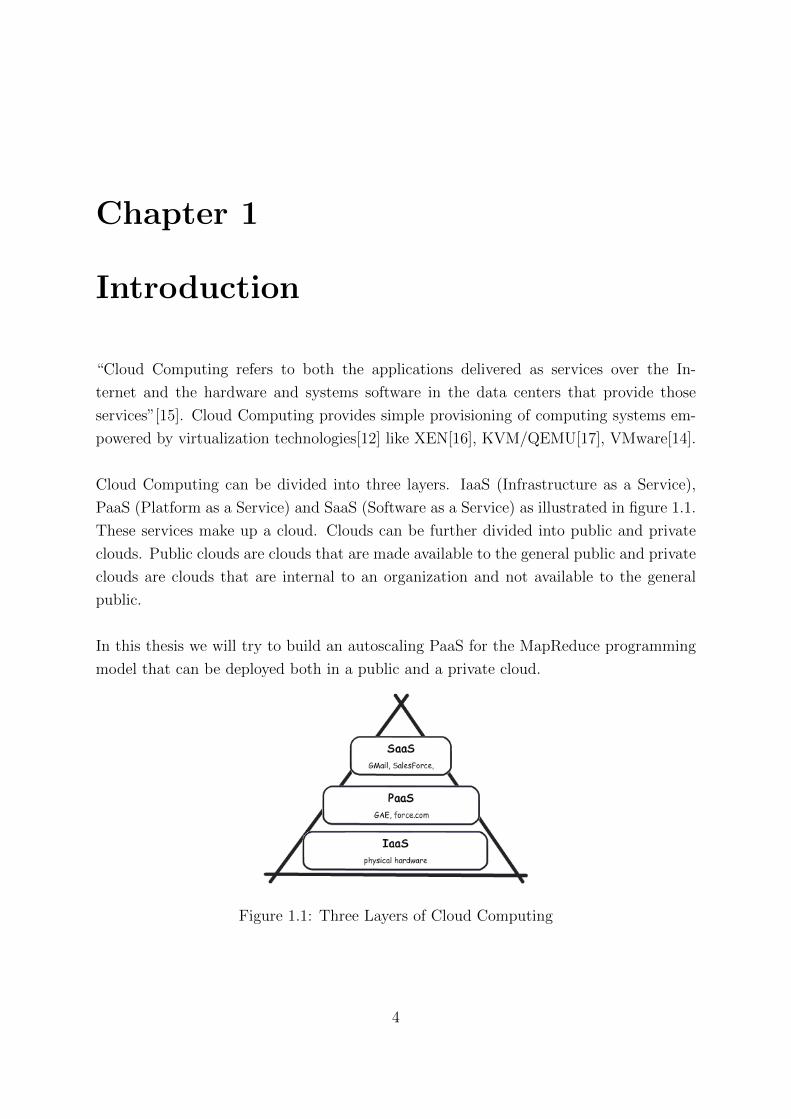
Cloud Computing can be divided into three layers. IaaS (Infrastructure as a Service),

PaaS (Platform as a Service) and SaaS (Software as a Service) as illustrated in figure 1.1.

These services make up a cloud. Clouds can be further divided into public and private

clouds. Public clouds are clouds that are made available to the general public and private

clouds are clouds that are internal to an organization and not available to the general

public.

In this thesis we will try to build an autoscaling PaaS for the MapReduce programming

model that can be deployed both in a public and a private cloud.

Figure 1.1: Three Layers of Cloud Computing

4

“MapReduce is a programming model and an associated implementation for process-

ing and generating large data sets”[21]. Users specify two functions, a map function that

processes key/value pairs and produces intermediate key/value pairs and a reduce func-

tion that merges those intermediate values.

The advantage of MapReduce is that the processing of the map and reduce operations

can be distributed and very often they can run in parallel. This means means that one

can dynamically increase the processing power of the underlying system by adding more

nodes and thus get results faster.

There are many implementations of MapReduce. One of them is the Apache Hadoop

project that develops open source software for reliable, scalable, distributed computing[8].

It includes an implementation of the MapReduce programming model, a distributed file

system and other subprojects to help run MapReduce jobs in a cluster of machines.

Running Hadoop on a cloud means that we have the facilities to add or remove com-

puting power from the Hadoop cluster within minutes or even less by provisioning more

machines or shutting down currently running ones. This gives us the elasticity to have

only the needed hardware for the job and not to waste CPU cycles on idling.

We will prototype a system where this scaling is done automatically based on some

rules and without any human intervention. We will present the full software stack of this

autoscaling framework, starting from the machine images to the autoscaling prototype.

1.1 Goals

Our main goal is to build a dynamic MapReduce cluster using the Hadoop implementa-

tion. The cluster will scale itself based on the load of the cluster. The cluster can be run

both in a public and a private cloud. We also want to monitor and debug the cluster in

real time to find out a good autoscaling strategy or to tune it. Our prototype system and

framework will consist of:

• Control panel or a dashboard to monitor a Hadoop cluster in real-time and debug

for possible problems.

• Virtual machine images for the Hadoop nodes. The images are preconfigured Linux

operating systems that automatically start Hadoop software on boot. The nodes

will automatically join a Hadoop cluster and report performance metrics to the

Control Panel.

5

• Identifying and collecting system metrics of the running nodes to the Control Panel

to make assessments of the load and health of the cluster.

• Providing an autoscaling strategy to scale the cluster horizontally based on the

monitored performance metrics of the cluster.

We will refer to all of these together as an autoscaling Hadoop cluster. The results will be

deliverables of different types. All the relevant custom configuration files and scripts are

in our version control repository at svn://dougdevel.org/scicloud/trunk/enter/.

1.2 Prerequisites

This thesis requires the user to have some basic understanding of cloud computing,

MapReduce and computer networks. These concepts are described in more detail in

chapter 2. If one is familiar with these concepts she can skip to chapter 3.

1.3 Outline

We will build and prototype the autoscaling cluster step by step, from building the ma-

chines, configuring Hadoop, extracting metrics and collecting them. We need to analyze

the performance metrics and then build the actual autoscaling framework.

• Chapter 2 describes all the background knowledge that we will use in building the

cluster. It will explain the IaaS services that we will be using for both the public

and private clouds, the architecture of the Apache Hadoop Project and also some

limitations that we need to consider when building our cluster.

• Chapter 3 describes the technical details of our cluster. Building the virtual ma-

chines, configuring the software, monitoring the performance metrics and building

our autoscaling framework.

• Chapter 4 outlines the future work that can be done based on this thesis and results.

We have built an autoscaling Hadoop cluster but there are many aspects that we

did not give enough attention and the framework we developed was more of a proof

of concept than an actual product.

6

Chapter 2

Background Knowledge

We chose Amazon Web Services (AWS)[6] as our public cloud provider and the Eucalyptus

private cloud software running at the Scientific Computing on the Cloud (SciCloud)[33]

at the University of Tartu as our private cloud provider, which is studying the scope of

establishing private clouds at universities[32].

We chose the Apache Hadoop project as the MapReduce implementation because it is

open source software, platform agnostic and there is plenty of documentation available

for installing, configuring, debugging and running a Hadoop installation.

2.1 IaaS Software

The AWS provides many different services of which we will be using just a few. As we

are also targeting the private cloud we cannot choose all the services from the AWS stack

as there are many that do not have an equivalent service in Eucalyptus[29], our private

IaaS software stack. Eucalyptus tries to be AWS compliant in terms of the services they

provide and also the APIs they provide.

2.1.1 Amazon Services

Amazon EC2

In 2006 Amazon announced a limited beta of Amazon Elastic Compute Cloud (EC2)[7].

The service allows users to rent virtual computers (servers) and run the desired operating

systems and applications on top of them. They also provide web services through which

users are able to boot, configure1 and terminate these machines. End users are paying

for the service based on how many hours a server is running.

1There are AWS services that can be attached to currently running instances.

7

To boot a server the user needs to create an Amazon Machine Image (AMI). AMI is

a compressed, encrypted, signed and split file system2 that can be booted into a running

instance on the Amazon Elastic Compute Cloud. A large preconfigured boot disk that

is split into pieces before boot. One can start as many AMIs she wishes and terminate

them whenever she sees fit. Instances of the AMIs do not not have any persistent storage

and all state is lost upon stopping an instance. AMIs do not come with a kernel but

instead they reference a kernel supported by the Amazon infrastructure. An AMI can be

run with almost any of the approved kernels available.

Amazon S3

Amazon S3 (Simple Storage Service) is an online storage offered by Amazon and provides

unlimited storage via a web service interface. Users can issue HTTP PUT and GET requests

to query and store objects in the storage. Amazon S3 is reported to store more than 102

billion objects as of March 2010[5].

Amazon S3 is built with a minimal feature set that includes writing, reading and deleting

objects containing from 1 byte to 5 gigabytes of data each. Each object is stored in a

bucket (like a folder) and the bucket can be stored in one of the available geographical

regions to minimize latency, costs or address regulatory requirements.

AMI files can be stored in the Amazon S3. Booting an AMI means querying the S3

to fetch the splits of the compressed, encrypted and signed file system and then booting

the re-assembled pieces. Storing an AMI in the S3 is a matter of creating a bucket and

uploading the splits as objects into the bucket.

Amazon EBS

Amazon Elastic Block Store (EBS) provides block level storage volumes for use with

Amazon EC2 instances. “Amazon EBS volumes are off-instance storage that persists

independently from the life of an instance”[9].

An EBS volume can be created of almost arbitrary size (1 GB to 1 TB) and then attached

to a running instance of an AMI. For the operating system an EBS volume looks like a

regular block device which can be partioned in any ways necessary and then formatted

with a desired file system.

2The file system image is split into n smaller pieces and all the pieces are stored instead of the one

large image file.

8

The EBS volumes can also be used as boot partitions for amazon AMIs. This pro-

vides support for larger AMI sizes (up to 1 TB) and also faster boot times. This means

that the AMI is not stored in S3 as a split file system but instead as block storage.

Amazon CloudWatch

Amazon CloudWatch[3] provides monitoring for cloud resources. For EC2 instances it is

possible to get CPU, disk and networking metrics in real-time of the running instances

and also historical data is made available to learn about usage patterns.

The key metrics that CloudWatch monitors are:

• CPU utilization, the percentage of the CPU(s) that are currently in use.

• The number of bytes received and sent on all network interfaces.

• Completed write and read operations to all disks to identify the rate at which the

instance is writing/reading to disks.

• The number of bytes written and read from all disks to identify the volume of the

data the instance is writing/reading to disks.

These metrics are read at an interval (every minute is the maximum frequency) from the

nodes and besides just aggregating the raw data, CloudWatch also provides the minimum,

maximum, sum, average and samples of the data for any given period that the service

has been active.

Amazon AutoScaling

Amazon offers a simple autoscaling[2] API to automatically horizontally scale your EC2

instances based on some predefined conditions. The API is called AutoScaling. This

means that Amazon will monitor the system metrics (using Amazon CloudWatch) and

based on some conditions of the metrics will boot more instances or terminate some of

the running instances.

The Amazon AutoScaling introduces couple of concepts that are used when defining

an autoscaling cluster.

AutoScalingGroup represents an application on the cloud that can horizontally scale.

The group has the minimum and maximum number of instances defined. It also has

a Cooldown defined which is the amount of time after a scaling activity completes

before any further autoscaling can happen.

9

Launch Configuration defines the EC2 instance that will be used to scale the Au-

toScalingGroup. It is a combination of an AMI and the configuration of the instance

(CPU, RAM, etc.).

Trigger mechanism has defined metrics and thresholds that initiate scaling of the Au-

toScalingGroup. A Trigger consists of a Period and a BreachDuration. The Period

controls how often Amazon CloudWatch measures the metrics and BreachDuration

determines the amount of time a metric can be beyond its defined limit before the

Trigger fires.

Tools

Amazon cloud services are exposed as a collection of web services. They are accessed

over the HTTP using REST (REpresentational State Transfer) and SOAP[23] protocols.

Amazon offers libraries for many different programming languages and platforms. The

bare minimum package is called ec2-tools and those shell command are sufficient to

manage a cluster (boot and terminate instances, manage storage, networking etc.).

There are numerous tools out there that gives users the functionality of provisioning

computing power and managing their storage with a click of a button instead of running

multiple commands in the command line interface. Either browser plugins or command-

line tools, they are front-ends to the public web services.

2.1.2 Eucalyptus Services

Eucalyptus is an open source software framework for cloud computing. It was first in-

troduced in 2009 and one of the main reasons behind the creation of it was that all

main cloud providers were and are still closed systems with open interfaces. The tools

for researchers interested in pursuing cloud-computing infrastructure were mostly missing.

“The Eucalyptus software package gives the users the ability to run and control entire

virtual machine instances deployed across a variety physical resources”[29]. Compared to

other open offerings (Usher[27], Enomalism[10]) Eucalyptus was designed to be as easy

to install and as non-intrusive as possible to resource needs. Small scale experiments can

be run off of a laptop.

Eucalyptus Equivalent Services

Eucalyptus machine images are quite similar to Amazon AMIs. They are compressed,

encrypted, split file systems containing the operating system. They do need different

10

kernel modules as the underlying IaaS system is different from AWS but the changing

of modules can be achieved by mounting the machine image and making appropriate

changes to them.

“The Eucalyptus cloud computing system has implemented exactly the same interface

as Amazon EBS based on the ATA over Ethernet[19] (AoE) technology”[4]. This makes

data transmission over the network quite efficient as AoE runs directly on Ethernet and

no TCP/IP overhead incurs. This approach does require that the disk volume server and

the node using the volume both to be in the same LAN or at least in the same VLAN.

Walrus is a storage service bundled with Eucalyptus that is interface compatible with

Amazon’s S3. This means that one can use Amazon tools or other Amazon compliant

tools to interface with Walrus. We will be using Walrus to store our private cloud AMI

files.

There is no CloudWatch equivalent in the Eucalyptus software stack. We emulated this

via custom metrics gathering explained in section 3.2.2 and for visualization of metrics

used a generally available monitoring tool called Ganglia[26] which is used for monitoring

high-performance systems such as clusters and grids(this is explained in more detail in

section 3.2.3).

There is no AutoScaling equivalent in the Eucalyptus software stack. We emulated this

by hard coding the minimum and maximum number of nodes into our custom autoscaling

framework. We did borrow the concepts of period and breach duration and cooldown in

our custom autoscaling framework.

Our experience shows that most tools that work with AWS are not feature complete

when using them with Eucalyptus services. We stumbled upon many occasions where

only a very specific version of a tool would work with Eucalyptus and then with lim-

ited functionality. Also while Amazon web services have GUIs for most tasks then with

Eucalyptus you need to use the command line interfaces.

2.1.3 Access Credentials

There are three types of access credentials that can be used to authenticate client’s

requests to the AWS and Eucalyptus services. We will be using two of them.

Access keys are to make secure REST requests to any AWS/Eucalyptus service APIs.

The access key consists of a Access Key ID and a Secret Access Key. All re-

quests include the Access Key ID in a readable format and it identifies the person

11

making the request. The Secret Access Key should be kept in private and is

only known to the AWS/Eucalyptus and to the person making the request. All

requests are signed with this Secret Access Key and AWS/Eucalyptus checks the

signature on every request.

Key Pair is a pair of a public and a private key that are associated with a name. This

key pair is required to connect to the EC2 instances via SSH. When creating an

AMI, the public key is put in there by AWS/Eucalyptus and only the holder of the

private key has access to that machine initially.

2.2 MapReduce and Apache Hadoop

2.2.1 MapReduce

The MapReduce programming model to support distributed computing on large data sets

on clusters of computers is patented by Google Inc. and was first published in 2004, the

patent was granted in 2010[20]. In this programming model users specify a map function

that iterates key/value pairs to produce a set of intermediate key/value pairs and also a

reduce function that will merge all intermediate values associated with the same inter-

mediate key.

Programs written in this manner can easily be run in a special MapReduce runtime

in such a way that partitioning input data, scheduling execution across the cluster, han-

dling machine failures and inter-machine communication are all managed and provided

by the runtime and is hidden from the developer of the algorithm.

The advantage of MapReduce is that the processing of the map and reduce operations

can be distributed and very often they can run in parallel. This means that one can dy-

namically increase the processing power of the underlying system by adding more nodes

and thus get results faster.

Today there are many implementations of MapReduce, both commercial and open source.

The original Google framework was written in C++, todays implementations include

Java, Ruby, Python, Erlang and many others. There is an implementation of MapRe-

duce that runs on GPUs[24] instead of CPUs.

In 2004 when the paper on MapReduce was published, already hundreds of programs

had been implemented in this fashion and thousands of MapReduce jobs were executed

on Google’s clusters every day[21]. In 2008 Yahoo! announced launching the world’s

12

largest Hadoop production application with more than 10 000 CPU cores[1]. From the

same year Facebook stated to have multiple Hadoop clusters, the biggest having 2500

CPU cores and 1 PB of disk space.

2.2.2 Apache Hadoop

Apache Hadoop is an implementation of MapReduce. Google licensed the patent of

MapReduce to the Apache Software Foundation and it was made public on one of

Apache’s mailing lists in April 2010[11].

The project consists of multiple sub-projects of which we will be using just a few. They

are (listed from [8]):

Hadoop Common consists of the common utilities that support the other Hadoop sub

projects.

MapReduce is a software framework for distributed processing of large data sets on

compute clusters.

HDFS is a distributed file system that provides high throughput access to application

data.

A simple Hadoop cluster consists of n ≥ 1 machines running the Hadoop software. The

cluster is a single master cluster with varying number of slave nodes. All slave nodes

besides computing MapReduce jobs also act as data replication stores. This follows the

approach that it is more cost-effective and time-efficient to move computing closer to

data than moving data closer to the computation.

Hadoop MapReduce

The Hadoop master runs a daemon called JobTracker. Users submit their MapReduce

jobs to this daemon. The JobTracker redistributes these jobs to the slave nodes where a

daemon called TaskTracker runs. The JobTracker tries to make sure that it pushes the

work to the TaskTrackers that are closest to the data of that task to avoid unnecessary

IO operations.

Hadoop Distributed File System

The Hadoop Distributed File System (HDFS) is a distributed file system designed to run

on commodity hardware[18]. HDFS is highly fault-tolerant, provides high throughput

access to application data and is suitable for applications that have large data sets.

13

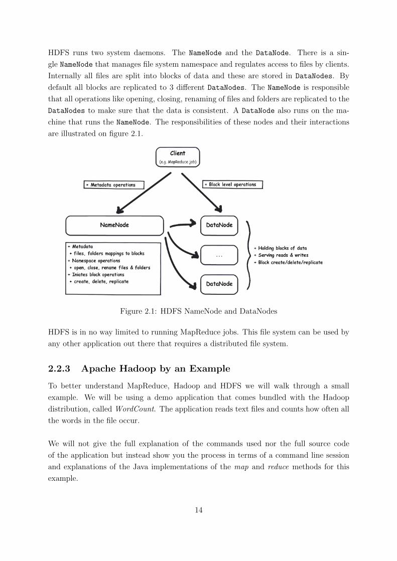
HDFS runs two system daemons. The NameNode and the DataNode. There is a sin-

gle NameNode that manages file system namespace and regulates access to files by clients.

Internally all files are split into blocks of data and these are stored in DataNodes. By

default all blocks are replicated to 3 different DataNodes. The NameNode is responsible

that all operations like opening, closing, renaming of files and folders are replicated to the

DataNodes to make sure that the data is consistent. A DataNode also runs on the ma-

chine that runs the NameNode. The responsibilities of these nodes and their interactions

are illustrated on figure 2.1.

Figure 2.1: HDFS NameNode and DataNodes

HDFS is in no way limited to running MapReduce jobs. This file system can be used by

any other application out there that requires a distributed file system.

2.2.3 Apache Hadoop by an Example

To better understand MapReduce, Hadoop and HDFS we will walk through a small

example. We will be using a demo application that comes bundled with the Hadoop

distribution, called WordCount. The application reads text files and counts how often all

the words in the file occur.

We will not give the full explanation of the commands used nor the full source code

of the application but instead show you the process in terms of a command line session

and explanations of the Java implementations of the map and reduce methods for this

example.

14

We will start off by creating a folder on the HDFS by issuing a command hadoop

dfs -mkdir our-input-folder. This will create a folder our-input-folder on the

HDFS and it will get replicated to multiple nodes on the cluster. We will copy some

files from the local file system to the HDFS by issuing hadoop dfs -copyFromLocal

my-books our-input-folder. This will copy the folder my-books to the HDFS folder

our-input-folder. Our map and reduce jobs will read the data from the HDFS and the

folder our-input-folder will contain the necessary books in which we want to count all

the words.

Implementing the Map and Reduce Methods

Next we will implement the actual map and reduce methods. In listing 2.1 we have the

Java implementation of the map method. Once the method is called with a key and

value, the key is disregarded and the value is split based on delimiters. The split values

are put into a key/value map, the keys will be the strings produced by the split and the

value will be a constant 1.

Listing 2.1: Map Method

1Text word = new Text ( ) ;

2// va lue − input to the Map method

3St r ing l i n e = value . t oS t r i ng ( ) ;

4// w i l l t o k en i z e based on d e l im i t e r charac t e r

5// se t , which i s ” \ t \n\ r\ f ” . De l imi t e r charac t e r s

6// w i l l not be tokens

7Str ingToken i ze r t o k e n i z e r = new Str ingToken i ze r ( l i n e ) ;

8while ( t o k e n i z e r . hasMoreTokens ( ) ) {9word . s e t ( t o k e n i z e r . nextToken ( ) ) ;

10// output i s a Map o f keys and va l u e s

11// one i s a cons tant 1

12output . c o l l e c t ( word , one ) ;

13}

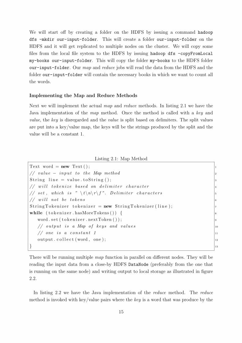
There will be running multiple map function in parallel on different nodes. They will be

reading the input data from a close-by HDFS DataNode (preferably from the one that

is running on the same node) and writing output to local storage as illustrated in figure

2.2.

In listing 2.2 we have the Java implementation of the reduce method. The reduce

method is invoked with key/value pairs where the key is a word that was produce by the

15

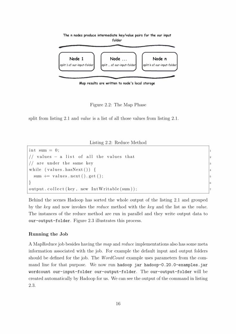
Figure 2.2: The Map Phase

split from listing 2.1 and value is a list of all those values from listing 2.1.

Listing 2.2: Reduce Method

1i n t sum = 0 ;

2// va lue s − a l i s t o f a l l the va lue s that

3// are under the same key

4whi le ( va lue s . hasNext ( ) ) {5sum += va lues . next ( ) . get ( ) ;

6}7output . c o l l e c t ( key , new IntWritab le (sum ) ) ;

Behind the scenes Hadoop has sorted the whole output of the listing 2.1 and grouped

by the key and now invokes the reduce method with the key and the list as the value.

The instances of the reduce method are run in parallel and they write output data to

our-output-folder. Figure 2.3 illustrates this process.

Running the Job

A MapReduce job besides having the map and reduce implementations also has some meta

information associated with the job. For example the default input and output folders

should be defined for the job. The WordCount example uses parameters from the com-

mand line for that purpose. We now run hadoop jar hadoop-0.20.0-examples.jar

wordcount our-input-folder our-output-folder. The our-output-folder will be

created automatically by Hadoop for us. We can see the output of the command in listing

2.3.

16

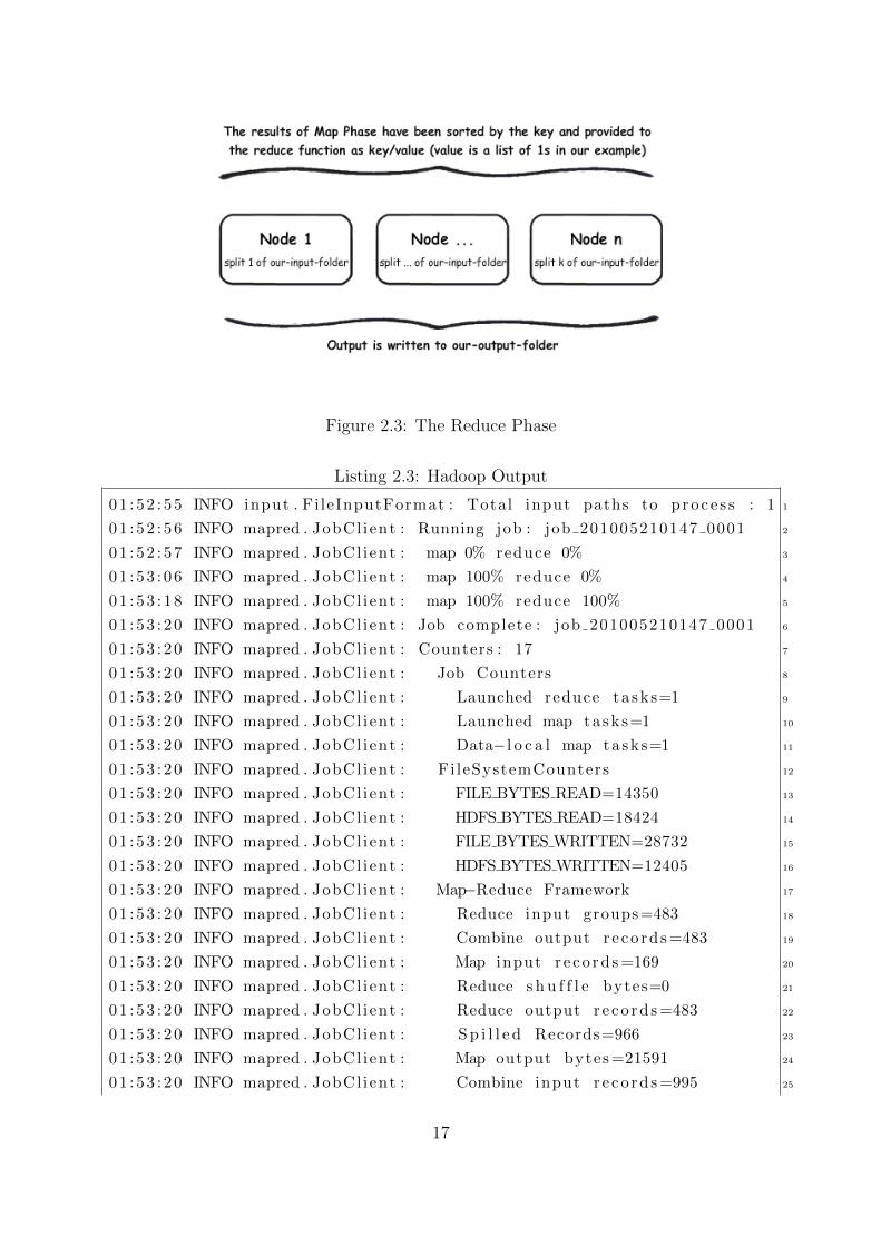
Figure 2.3: The Reduce Phase

Listing 2.3: Hadoop Output

101 : 52 : 55 INFO input . Fi leInputFormat : Total input paths to proce s s : 1

201 : 52 : 56 INFO mapred . JobCl ient : Running job : job 201005210147 0001

301 : 52 : 57 INFO mapred . JobCl ient : map 0% reduce 0%

401 : 53 : 06 INFO mapred . JobCl ient : map 100% reduce 0%

501 : 53 : 18 INFO mapred . JobCl ient : map 100% reduce 100%

601 : 53 : 20 INFO mapred . JobCl ient : Job complete : job 201005210147 0001

701 : 53 : 20 INFO mapred . JobCl ient : Counters : 17

801 : 53 : 20 INFO mapred . JobCl ient : Job Counters

901 : 53 : 20 INFO mapred . JobCl ient : Launched reduce ta sk s=1

1001 : 53 : 20 INFO mapred . JobCl ient : Launched map ta sk s=1

1101 : 53 : 20 INFO mapred . JobCl ient : Data−l o c a l map ta sk s=1

1201 : 53 : 20 INFO mapred . JobCl ient : Fi leSystemCounters

1301 : 53 : 20 INFO mapred . JobCl ient : FILE BYTES READ=14350

1401 : 53 : 20 INFO mapred . JobCl ient : HDFS BYTES READ=18424

1501 : 53 : 20 INFO mapred . JobCl ient : FILE BYTES WRITTEN=28732

1601 : 53 : 20 INFO mapred . JobCl ient : HDFS BYTES WRITTEN=12405

1701 : 53 : 20 INFO mapred . JobCl ient : Map−Reduce Framework

1801 : 53 : 20 INFO mapred . JobCl ient : Reduce input groups=483

1901 : 53 : 20 INFO mapred . JobCl ient : Combine output r e co rd s =483

2001 : 53 : 20 INFO mapred . JobCl ient : Map input r e co rd s =169

2101 : 53 : 20 INFO mapred . JobCl ient : Reduce s h u f f l e bytes=0

2201 : 53 : 20 INFO mapred . JobCl ient : Reduce output r e co rd s =483

2301 : 53 : 20 INFO mapred . JobCl ient : S p i l l e d Records=966

2401 : 53 : 20 INFO mapred . JobCl ient : Map output bytes =21591

2501 : 53 : 20 INFO mapred . JobCl ient : Combine input r e co rd s =995

17

2601 : 53 : 20 INFO mapred . JobCl ient : Map output r e co rd s =995

2701 : 53 : 20 INFO mapred . JobCl ient : Reduce input r e co rd s =483

To work with the actual results we need to copy a file created in the our-output-folder

to local disk and then read it. To find out the name of the file we can issue a hadoop dfs

-ls our-output-folder that will print the contents of the folder and then issue hadoop

dfs -cat our-output-folder/filename to quickly inspect it.

18

Chapter 3

Results

Our main goal is to build a dynamic MapReduce cluster using the Hadoop implementa-

tion. The cluster will scale itself based on the load of the cluster. The cluster can be run

both in a public and a private cloud. We also want to monitor and debug the cluster in

real-time to find out a good autoscaling strategy or to fine-tune one.

We chose Amazon Web Services (AWS) as our public cloud provider and the Eucalyptus

private cloud software running at the Scientific Computing on the Cloud (SciCloud) at

the University of Tartu as our private cloud provider.

We chose the Apache Hadoop project as the MapReduce implementation because it is

open source software, platform agnostic and there is plenty of documentation available

for installing, configuring, debugging and running a Hadoop installation.

Our results will be of production quality on the AWS and of testing quality on the

SciCloud. This is mainly due to the fact that SciCloud Eucalyptus cluster is still in beta

phase and it was easier to fine tune our AMIs in a production level IaaS. It was also

possible to provision more machines at a time in AWS than currently available in the

SciCloud infrastructure.

3.1 Autoscalable AMIs

3.1.1 Requirements

To run a Hadoop cluster we will need at least two AMI files. One to act as the Hadoop

master and one to act as a Hadoop slave. We require that only one Hadoop master is

running at a time and that is is always started before a single Hadoop slave has been

booted.

19

We do not require any human intervention to run the Hadoop cluster but we do want to

monitor the status of the cluster. We also might need to start the first master instance

manually when there are no instances running yet. For these reasons we define a web

service that we call the Control Panel. The Control Panel is running on a separate ma-

chine and is only accessible to the cluster via HTTP. We presume that the Control Panel

is constantly running.

Our architecture requires all AMI instances to start their Hadoop daemons (slaves start

slave daemons, master starts master daemons) on boot time and then inform the Control

Panel of their status. We also require them to send a heartbeat to the Control Panel to

have an overview of the size of the cluster and its load.

We require that our Hadoop cluster is dynamic, e.q whenever a new Hadoop slave node

is booted, it joins the already running cluster after boot without any human intervention.

We require that all instances have ample disk space at their disposal. First option would

be to make our AMIs large enough for the Hadoop data but this would also slow down

the booting of the AMIs significantly. The storage needs to be external to the AMIs.

We also require that the AMIs do not depend on a specific AWS or Eucalyptus user

and the cluster can be set up by any user by just configuring her access credentials (see

section 2.1.3) at the Control Panel.

Our end goal is to have AMIs that require no human intervention to boot or terminate

themselves. No human intervention shall be required to even create or join the Hadoop

cluster. All is managed by the startup procedures of the AMIs and we can monitor the

success of this from the Control Panel.

3.1.2 Meeting the Requirements

The Master and Slave AMIs

We chose Linux as for the underlying operating system. On the AWS we built our im-

ages using Debian 5.0 and on the Eucalyptus we chose Ubuntu 9.0. On Eucalyptus we

chose Ubuntu instead of Debian because of the easier setup of Ubuntu in the Eucalyptus

environment.

We are running the latest Hadoop stable release which is 0.20.2 at this moment. We

20

Table 3.1: System Services Running on Nodes

Master node Slave node

TaskTracker TaskTracker

DataNode DataNode

JobTracker

NameNode

SecondaryNameNode

are using Java HotSpot 1.6.0 20 for running Hadoop. Our machines have 1.7 GB of

RAM and are single CPU core units. Besides Hadoop we have a minimal set of services

running and most of the resources are for Hadoop to use.

We constructed two AMIs for both Eucalyptus and AWS. One being the Hadoop master

and the other one the slave image. Hadoop wise the differences are the number of services

that are running. The different services on master and slave nodes are outlined in table

3.1.

Dynamic Scaling of a Hadoop Cluster

Hadoop has two types of slave configurations. One is to specify all slave IPs in a file on

the master instance. This provides a single location to add and remove slaves and also

control the life cycle of the slave daemons in one central place. A single command on the

master server can stop or start all the slaves of the cluster.

The other approach is more dynamic and requires the slave to know the IP of the master

server. Once the TaskTracker and DataNode daemons are started on the slave node they

connect to the master node and let her know of their existence. The dynamic approach

does not provide a single location to control all the slave nodes but it does have the

feature of adding or removing slave nodes without making any configuration changes to

the master node.

In our configuration we chose the latter. This requires us to know the IP of the master

server before starting the slave instance. We achieve this by requiring that a master

instance is running before a single slave machine is started.

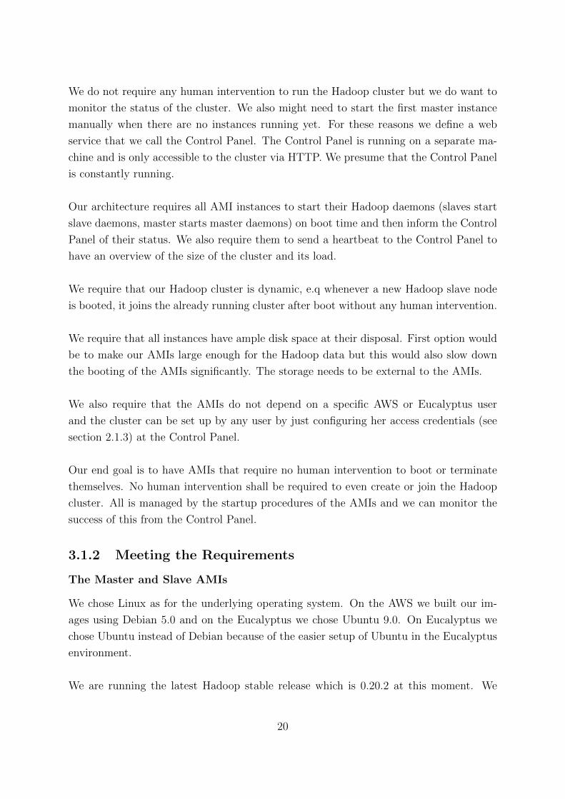
Once the master server starts it will report its IP to the Control Panel. Control Panel

will save this IP as the master IP. During boot time of the slave nodes, the slave nodes

will query the Control Panel for the master IP. The slave nodes will take this IP and

21

update its system configuration to reflect that this is the IP of the master and then start

the Hadoop services. This is illustrated in figure 3.1.

We implemented this IP sharing by using a host, named master in all our Hadoop

configuration files and then updated the IP of that host in the /etc/hosts file. During

the booting of the slave machine it queries the Control Panel for the IP address of the

master Hadoop instance and upon receiving the IP it writes a line to its /etc/hosts file

and then start the Hadoop services.

Figure 3.1: Startup of Master and Slave Instances

Ample Disk Space

To keep our AMIs as small as possible we will be using external storage to facilitate the

needs of data storage. For the storage we will be using EBS volumes. The creating and

managing of the EBS volumes will be handled by the Control Panel and instances will

talk to the Control Panel via web service to request the volume.

When an instance boots it will notify the Control Panel that it is in need of external

storage. The Control Panel will then create the volume and attach it to the instance that

requested the volume. The instance will poll the Control Panel until it gets notified that

the volume has been successfully created and attached. Figure 3.2 illustrates the process.

The instance will then mount the attached disk, format it with a file system and then

create the necessary folder structure for Hadoop. Once all this is done, Hadoop services

are started.

We used this approach only at the SciCloud due to the size limitations to the AMI

files (at the time of experimenting it was 2 GB). At AWS we used 20 GB EBS AMI files

and did not implement the attaching of external storage.

22

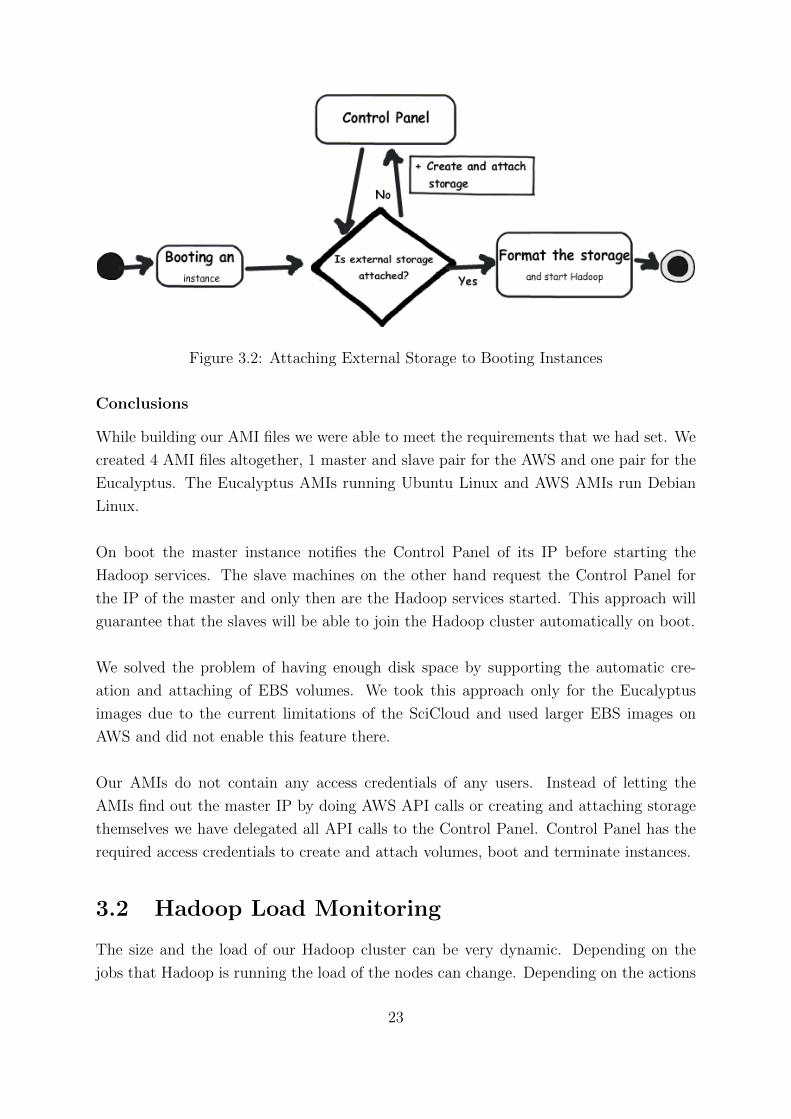
Figure 3.2: Attaching External Storage to Booting Instances

Conclusions

While building our AMI files we were able to meet the requirements that we had set. We

created 4 AMI files altogether, 1 master and slave pair for the AWS and one pair for the

Eucalyptus. The Eucalyptus AMIs running Ubuntu Linux and AWS AMIs run Debian

Linux.

On boot the master instance notifies the Control Panel of its IP before starting the

Hadoop services. The slave machines on the other hand request the Control Panel for

the IP of the master and only then are the Hadoop services started. This approach will

guarantee that the slaves will be able to join the Hadoop cluster automatically on boot.

We solved the problem of having enough disk space by supporting the automatic cre-

ation and attaching of EBS volumes. We took this approach only for the Eucalyptus

images due to the current limitations of the SciCloud and used larger EBS images on

AWS and did not enable this feature there.

Our AMIs do not contain any access credentials of any users. Instead of letting the

AMIs find out the master IP by doing AWS API calls or creating and attaching storage

themselves we have delegated all API calls to the Control Panel. Control Panel has the

required access credentials to create and attach volumes, boot and terminate instances.

3.2 Hadoop Load Monitoring

The size and the load of our Hadoop cluster can be very dynamic. Depending on the

jobs that Hadoop is running the load of the nodes can change. Depending on the actions

23

of our autoscaling framework the size of the cluster can change. We want to monitor the

size and the performance metrics of our cluster.

We started out by requiring all the nodes to send a heartbeat every minute to the Control

Panel. This gives an overview of the number of slaves in the cluster and also the IP of

the current master.

We wanted to keep the heartbeat and the gathering of system performance metrics sep-

arate. This lets us replace one of the systems without changing the other. We started

reporting the metrics that were monitored in The Blind Men and the Elephant: Piecing

Together Hadoop for Diagnosis[31].

After collecting the metrics we realized that this is not enough. We need to visualize

the data, store historical data, run comparisons and monitor the cluster loads in real-

time. We upgraded our reporting to the Ganglia system. Now we were able to monitor

our cluster near real-time with automatic history and with graphs of the metrics gathered.

3.2.1 Heartbeat

We setup all our nodes to run a wget[28] against our Control Panel every minute via

cron[25]. The IP of the node and a boolean flag if this node is a master or not are

embedded into the request as GET parameters. At the Control Panel the request is logged

and the IP is entered with the master flag into a database. We say that the node is down

if the Control Panel has not heard a heartbeat from the node for 3 minutes.

3.2.2 System Metrics

We decided to gather the metrics that were gathered in [31]. In that thesis the metrics

were used to identify resource hogs, application hangs and also localize the fault to a

subset of of slave nodes in a Hadoop cluster. The metrics were:

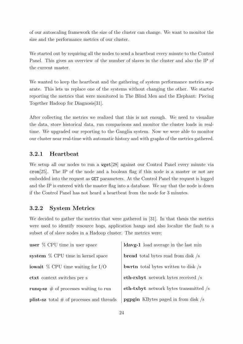
user % CPU time in user space

system % CPU time in kernel space

iowait % CPU time waiting for I/O

ctxt context switches per s

runq-sz # of processes waiting to run

plist-sz total # of processes and threads

ldavg-1 load average in the last min

bread total bytes read from disk /s

bwrtn total bytes written to disk /s

eth-rxbyt network bytes received /s

eth-txbyt network bytes transmitted /s

pgpgin KBytes paged in from disk /s

24

pgpgout KBytes paged out to disk /s

fault page faults (major + minor) /s

TCPAbortOnData # of TCP connec-

tions aborted with data in queue

rto-max Maximum TCP retransmission

timeout

To extract these metrics we used the the sar utility from the sysstat[22] package. We

wrote a Python daemon wrapper around the tool to report the metrics from the node,

accompanied by the IP of the node to our Control Panel. The metrics are sent every 30

seconds. The Control Panel saves all this information into a database with a timestamp

for later inspection.

After running tests (see section 3.3.1 and 3.3.2) on the cluster we extracted the sys-

tem metrics from the Control Panel and used everyday tools such as Microsoft Excel to

understand which metrics correlated to the cluster load and changes in the cluster size.

Hadoop is a complex piece of software and the MapReduce jobs vary a lot in CPU

and data needs that making assumptions based on these black box metrics weather to

add or remove nodes is a difficult task. Although running the same tests multiple times

on the same vanilla cluster we were not getting deterministic results.

We decided that we need to visualize the metrics in real-time to better understand

the load of the cluster while the tests are running. We moved on to Ganglia for the

performance metric analysis.

3.2.3 Ganglia

Ganglia is an open source software tool that monitors high-performance systems such as

clusters and grids. It consists of gmond, gmetad and a web front end. Gmond is a multi-

threaded daemon that runs on all the nodes and reports back information to gmetad.

Gmetad gathers the metrics, archives them and generates reports. It uses internally the

rrdtool[30] for data logging and graphing. The data is visualized by the web front end

bundled with Ganglia.

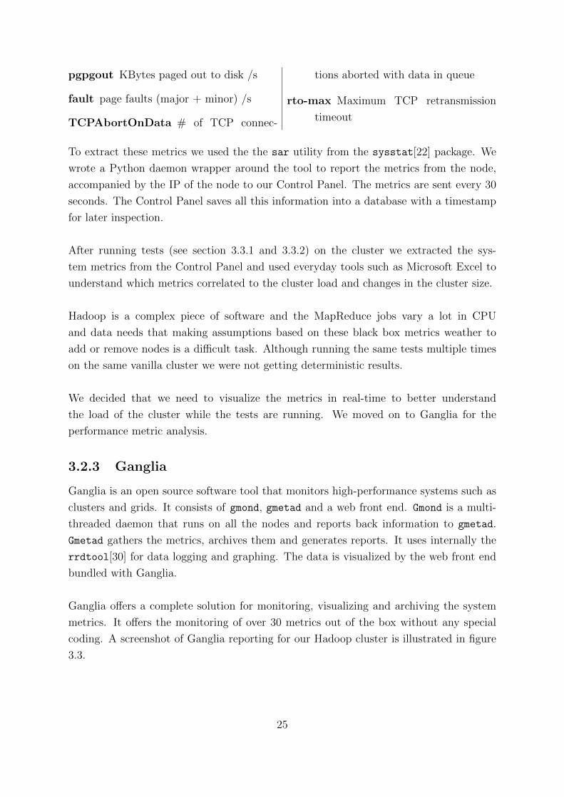
Ganglia offers a complete solution for monitoring, visualizing and archiving the system

metrics. It offers the monitoring of over 30 metrics out of the box without any special

coding. A screenshot of Ganglia reporting for our Hadoop cluster is illustrated in figure

3.3.

25

Figure 3.3: Screenshot of Ganglia

26

3.2.4 Amazon CloudWatch

Amazon also offers a service for monitoring the performance of an EC2 instance as ex-

plained in section 2.1.1. We did not consider this as an option because there is no

equivalent in the Eucalyptus software stack and we would like to target both platforms

with the minimum number of software tools and APIs.

3.2.5 Conclusions

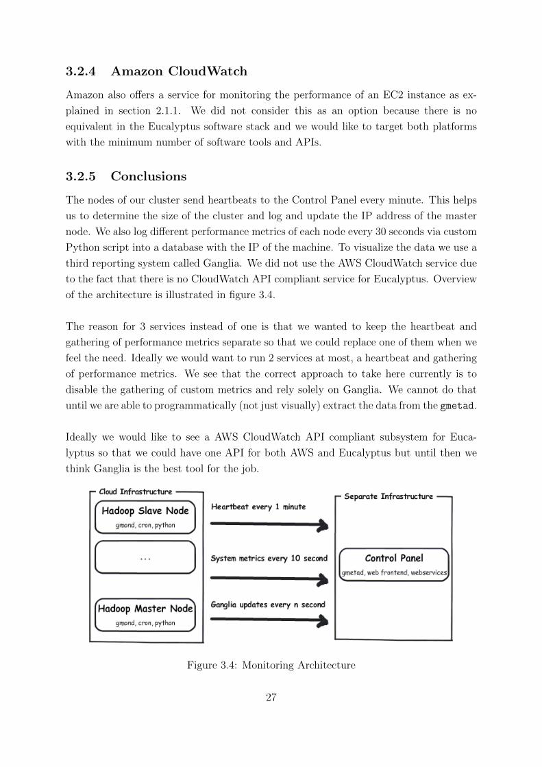
The nodes of our cluster send heartbeats to the Control Panel every minute. This helps

us to determine the size of the cluster and log and update the IP address of the master

node. We also log different performance metrics of each node every 30 seconds via custom

Python script into a database with the IP of the machine. To visualize the data we use a

third reporting system called Ganglia. We did not use the AWS CloudWatch service due

to the fact that there is no CloudWatch API compliant service for Eucalyptus. Overview

of the architecture is illustrated in figure 3.4.

The reason for 3 services instead of one is that we wanted to keep the heartbeat and

gathering of performance metrics separate so that we could replace one of them when we

feel the need. Ideally we would want to run 2 services at most, a heartbeat and gathering

of performance metrics. We see that the correct approach to take here currently is to

disable the gathering of custom metrics and rely solely on Ganglia. We cannot do that

until we are able to programmatically (not just visually) extract the data from the gmetad.

Ideally we would like to see a AWS CloudWatch API compliant subsystem for Euca-

lyptus so that we could have one API for both AWS and Eucalyptus but until then we

think Ganglia is the best tool for the job.

Figure 3.4: Monitoring Architecture

27

3.3 Generating Test Load

To observe real world system metrics and test our cluster we need to run real world

MapReduce jobs on it to generate load and disk utilization. We chose to use the HDFS

Synthetic Load Generator and the sort example both bundled with the Apache Hadoop

project.

3.3.1 HDFS Synthetic Load Generator

The Synthetic Load Generator (SLG) is designed for testing NameNode behavior under

different client loads. In our tests we used the default settings to generate the directory

structure and the random files. Then we ran the load generator and collected system

metrics. This test provides only HDFS level load generation, CPU is not involved and it

is mainly either disk IO or network IO.

3.3.2 Apache Hadoop Sort Benchmark

The Apache Hadoop Sort Benchmark consists of two steps. The first is to generate ran-

dom data. The default settings are to generate 1 TB of data. In our examples we tweaked

that to be 5 GB instead. This way we were able to run more tests in the same time frame

and we did not have to increase the storage size. The generating of 5GB data on a 4

node cluster takes about 10 minutes. The second step is to sort the data.

This benchmark gives a significant load to the cluster. Even on a small cluster (10

Hadoop Nodes) the load spiked as high as 20 on some nodes. It also introduces real

world like data transfer between the nodes and we were able to monitor different system

metrics of the nodes.

3.3.3 Identifying Relevant Metrics

Through our testing we recorded 15 000 entries from 80 different IP addresses in the

metrics table. We did not run any statistical analyzes on the data as we were not able

to get even similar cluster average loads when running the same MapReduce job on the

same data. We did choose the load average to be the metric to continue with in our

experiments and defining our autoscaling strategy.

3.3.4 Conclusions

We have configured our AMIs to be single CPU units that have 1.7 GB of RAM (the

AWS Small Instance) and 20GB of storage. The Hadoop configuration lets a single node

28

run up to 4 tasks, 2 map tasks and 2 reduce tasks.

Our observations show that an average load1 for this kind of node, when all task slots

are utilized is 10. This is large and we should decrease the number of slots per node or

increase the CPUs of the node.

Hadoop optimizes the jobs for highest efficiency, meaning that when it sees that a ma-

chine has 2 map task slots and 2 reduce task slots, it will use all of those when scheduling

jobs. It is up to us to configure the proper number of tasks that are suitable to the

hardware that we are running.

In table 3.2 we can see that these high loads do not produce consistent results. Mul-

tiple processes waiting for CPU2 time can have negative effects on the outcome due to

thread thrashing3.

Once we increased the number of nodes to 4 we did not see the sorting going any faster,

it ran actually slower. After 2 more runs we were able to get the time to be 24 minutes

which is 6 minutes faster than a single node run. Then we ran the same test with 10

nodes and observed a healthy decrease in time it took.

We also ran the same tests with instances that had 2 CPU cores. The outcome did

not differ much. A single run finished in 24 minutes, 4 node run was a little bit faster

and without the thrashing side effects. The 11 node run was just 1 minute faster than

compared to the 1 CPU core run. Our analysis of the results tells us that with proper

configuration of number of slots we can get more deterministic results and that there is

a point from which we cannot go any faster even if we increase the processing power by

two.

3.4 Autoscaling Framework

We built AMIs that on boot start the Hadoop services, we also configured the Hadoop

installations in a way that on start they join a cluster. On each node we also have

configured metric gathering to assess the load of the cluster from a central location. Now

we will put these all together into a autoscaling framework.

1Average number of processes waiting for the CPU or IO. Idle computer has a load 0, each waiting

process adds a 1.2We say CPU bound because we had defined 4 times more task slots than CPUs.3Program makes little progress because of the excessive context switching.

29

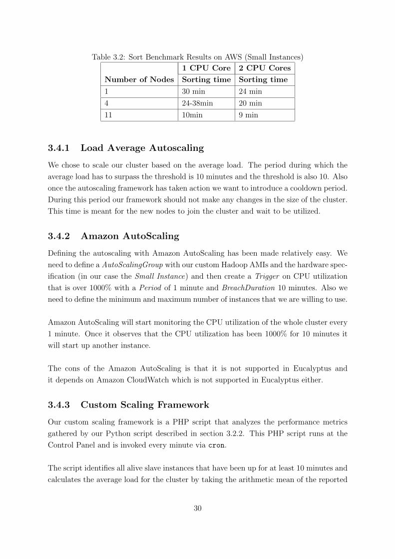
Table 3.2: Sort Benchmark Results on AWS (Small Instances)

1 CPU Core 2 CPU Cores

Number of Nodes Sorting time Sorting time

1 30 min 24 min

4 24-38min 20 min

11 10min 9 min

3.4.1 Load Average Autoscaling

We chose to scale our cluster based on the average load. The period during which the

average load has to surpass the threshold is 10 minutes and the threshold is also 10. Also

once the autoscaling framework has taken action we want to introduce a cooldown period.

During this period our framework should not make any changes in the size of the cluster.

This time is meant for the new nodes to join the cluster and wait to be utilized.

3.4.2 Amazon AutoScaling

Defining the autoscaling with Amazon AutoScaling has been made relatively easy. We

need to define a AutoScalingGroup with our custom Hadoop AMIs and the hardware spec-

ification (in our case the Small Instance) and then create a Trigger on CPU utilization

that is over 1000% with a Period of 1 minute and BreachDuration 10 minutes. Also we

need to define the minimum and maximum number of instances that we are willing to use.

Amazon AutoScaling will start monitoring the CPU utilization of the whole cluster every

1 minute. Once it observes that the CPU utilization has been 1000% for 10 minutes it

will start up another instance.

The cons of the Amazon AutoScaling is that it is not supported in Eucalyptus and

it depends on Amazon CloudWatch which is not supported in Eucalyptus either.

3.4.3 Custom Scaling Framework

Our custom scaling framework is a PHP script that analyzes the performance metrics

gathered by our Python script described in section 3.2.2. This PHP script runs at the

Control Panel and is invoked every minute via cron.

The script identifies all alive slave instances that have been up for at least 10 minutes and

calculates the average load for the cluster by taking the arithmetic mean of the reported

30

ldavg-1. If this value is greater than 10 we will launch 3 more instances but not exceeding

our defined maximum which is 10 in our case. For the next 15 minutes there will be a

cooldown period when our PHP script will not take any action. This will give time for

the new instances to boot and join the cluster and start working. The logic is illustrated

in figure 3.5.

Figure 3.5: Autoscaling Logic

3.4.4 Scaling the Cluster Down

So far we have only looked at increasing the size of the cluster and we have not men-

tioned scaling down. We do not want waste resources and it is a logically step to scale

our clusters down when there is not enough load.

Our naive approaches of shutting down slave nodes after a period of low load of the

cluster resulted in inconsistent data in the HDFS. This was due to the fact that each

node holds a piece of the data and the default configuration is to have 3 replicas of each

block. Once the 3 nodes holding those replicas are shutdown the data is lost.

The safest way is to turn off instances one by one and after every turned off instance

notifying the NameNode about the decommissioned node. There is also an administrative

tool balancer provided with the Apache Hadoop project that can be used to re-balance

a changed cluster.

31

3.4.5 Apache Hadoop and Cluster Changes

We ran the same tests as described in section 3.3.4 with a dynamic cluster. The cluster

was already running and had 4 nodes. The nodes were sorting 5 GB of data and all the

map tasks had already finished. Our autoscaling framework added 3 nodes to the cluster

that had already for 11 minutes been sorting data.

We observed that the moment the 3 nodes had joined the cluster there were 7 reduce

tasks running on the 4 nodes. Hadoop started copies of the same running reduce tasks

on the new nodes to utilize the new nodes.

This shows how inefficient it is to autoscale a Hadoop cluster based on the load. Now we

had 7 nodes of which 5 were running the same reduce tasks competing with each other.

This also shows that there is room for tweaking the strategies of MapReduce implemen-

tations on how to act to cluster size changes. The new nodes can be used for jobs in the

queue instead of competing with each other.

3.4.6 Conclusions

We decided to scale our cluster based on the average load of the cluster. If the average

load of the cluster exceeds a limit for a duration of some time the cluster will resize by n

number of nodes and then wait for a period of time before taking any further action to

give the cluster time to start to utilize the newly added nodes.

It is really difficult to efficiently scale a Hadoop cluster based on the average load or

even based on any other black box performance metric. Hadoop will schedule its jobs for

maximum efficiency of the cluster. This means that even when the size of the cluster is

increased Hadoop will divide the computations for a larger set of nodes and will make

sure that all of them are fully utilized.

More important to efficient scaling are the white box metrics of a Hadoop cluster. In this

thesis we have not gathered them but when running the tests we have observed them and

seen that knowing the queue size of the cluster can greatly benefit the decision made by

an autoscaling framework. For example if the load of the cluster is 10 but there are only 5

reduce tasks running and the size of the cluster is also 5 our framework will launch 3 more

instances. If we knew that there are no more jobs in the queue we would not start those 3.

Scaling down a Hadoop cluster is not an easy task as all nodes also hold a portion

of the data in the HDFS and we do not want to introduce data loss. There is no easy

32

way to scale down by terminating multiple instances at a time but there are ways to scale

down the cluster by taking nodes offline one by one and then between the steps forcing

data replication to other nodes.

33

Chapter 4

Future Work

4.1 Hadoop Autoscaling as a Scalr Module

Scalr[13] is an open source framework that scales web infrastructure. One can define a

website that she wants to scale then describes the infrastructure that she is willing to use

to run that website. The she can choose between different scaling options.

• Scaling based on the time and day of the week

• Scaling based on bandwidth usage

• Scaling based on load averages

• Scaling based on SQS queue size

• Scaling based on RAM usage.

Scalr will use the chosen strategy to autoscale the website. The metrics will be extracted

from the load balancer instance that is in front of the website using the AWS CloudWatch

service.

We think that it is relatively easy to add Hadoop support into Scalr. We have already

created the necessary autoscaling AMIs that Scalr needs to boot and terminate. We still

would need to enhance Scalr to use other performance metrics providers than just Cloud-

Watch and then define Hadoop specific strategies for the scaling. Supporting Eucalyptus

IaaS instead of just AWS would make this software stack fully open source and free of

charge for a private cloud.

We also think that the combination of this software stack (Eucalyptus + Scalr + Gan-

glia + Hadoop + Scaling framework) can be offered as a product to companies that use

34

MapReduce to analyze their data. It will provide an easy management of the platform

and can make more effective use of the underlying resources.

4.2 White Box Metrics

In this thesis we only looked at black box metrics and did not consider any white box

metrics from the running Hadoop processes. Hadoop offers out of the box different metrics

of the running processes, they are organized into contexts. The contexts are:

jvm context contains basic JVM stats. Memory usage, thread counts, garbage collection,

etc.

dfs context contains NameNode metrics of the file system. The capacity of the file system,

number of files, under-replicated blocks, etc.

mapred context contains JobTracker and TaskTracker counters such as how many

map/reduce operations are currently running or have run so far. How many jobs

have been submitted, how many completed, etc.

These metrics can also be valuable to working out Hadoop specific autoscaling strategies.

Ganglia has a Hadoop extension that lets Hadoop feed these metrics into the Ganglia

system. This gives an easy way to monitor and visualize these metrics without any

significant changes to the AMI files.

35

Conclusions

We have presented our framework for autoscaling Hadoop clusters based on the perfor-

mance metrics of the cluster. The framework will gather heartbeats, performance metrics

and based on the data start more instances. Hadoop will start using the new instances

and jobs get executed faster.

We have created and configured AMI files that are full featured Linux installations ready

to run on either a public cloud infrastructure (AWS) or on a private cloud infrastructure.

The AMIs setup the heartbeats, metric reporting, Hadoop startup and cluster joining

automatically during boot time.

We have also created a set of web services called the Control Panel that handle met-

ric logging, help Hadoop nodes join the cluster, attach external storage and provide an

overview of the cluster.

As future work we see that proper autoscaling for a Hadoop cluster is not based on

a black box performance metric but based on a combination of white box metrics and

black box metrics. Hadoop exposes many metrics that can be used to predict the work

load of a cluster and thus make better adjustments to the size of the cluster to facilitate

the increasing or decreasing demand.

We also see that the open source software stack Eucalyptus, Hadoop, Ganglia and Scalr

in combination can be commercialized into a product. Scalr would serve as front-end for

end users to configure their cluster size and type and also the required scaling strategy.

Eucalyptus would provide the IaaS services running Hadoop. Ganglia would be handling

all the metric extraction.

36

Autoscaling Hadoop Clusters

Toomas Romer

Magistritoo

Kokkuvote

Pilve arvutused on viimaste aastate jooksul palju koneainet pakkunud. Alates sellest, et

tegemist ei ole millegi muuga kui virtualiseerimine ilusa nimega, kuni selleni, et tulevik

on pilve arvutuste paralt. Juba 4 aastat on virtuaalsed serverid, andmehoidlad, andme-

baasid ja muud infrastruktuuri elemendid olnud kattesaadavad veebiteenustena.

Aastal 2004 avaldas Google artikli, mis kirjeldas, kuidas Google suuri arvutiparke efek-

tiivselt suurte andmehulkade analuusimiseks kasutab. Nad olid ehitanud platvormi, kus

algoritmid, mis olid vaga kindla ulesehitusega programeeritud, jooksid hajutatult ja par-

alleelselt ilma, et algoritmi arendaja oleks eksplitsiitselt nendele aspektidele rohunud.

Google nimetas oma lahenemist MapReduceks. Tanaseks on tekkinud mitmeid imple-

mentatsioone sellele platvormile.

Antud toos me ehitame ise sklaleeruva MapReduce platvormi, mis baseerub vabalahtekoodiga

tarkvara Apache Hadoop projektil. Antud platvorm skaleerib end ise, vastavalt serverite

koormatusele kaivitab uusi servereid, et kiirendada arvutusprotsessi.

Tooga on kaasas nii Amazon kui ka Eucalyptus pilve teenustele sobivad Linuxi instal-

latsioonide tommised, mis on konfigureeritud automaatselt raporteerima enda koormust

ning uhinema juba olemasoleva MapReduce arvutusvorguga. Koik relevantsed konfigurat-

siooni failid ning skriptid on kattesaadavad versioonihalduse repositooriumist aadressil

svn://dougdevel.org/scicloud/trunk/enter/hadoop/trunk/.

37

Bibliography

[1] Apache Hadoop. http://developer.yahoo.net/blogs/hadoop/2008/02/

yahoo-worlds-largest-production-hadoop.html, May 2008.

[2] Amazon Auto Scaling Developer Guide. http://awsdocs.s3.amazonaws.com/

AutoScaling/latest/as-dg.pdf, May 2009.

[3] Amazon CloudWatch Developer Guide. http://awsdocs.s3.amazonaws.com/

AmazonCloudWatch/latest/acw-dg.pdf, May 2009.

[4] Supporting Cloud Computing with the Virtual Block Store System, Oxford UK, 12/9-

11/2009 2009.

[5] Amazon S3 Now Hosts 100 Billion Objects. http://www.datacenterknowledge.

com/archives/2010/03/09/amazon-s3-now-hosts-100-billion-objects/, May

2010.

[6] Amazon Web Services. http://aws.amazon.com/, May 2010.

[7] Amazon Web Services Blog: Amazon EC2 Beta. http://aws.typepad.com/aws/

2006/08/amazon_ec2_beta.html, May 2010.

[8] Apache Hadoop. http://hadoop.apache.org/, May 2010.

[9] Elastic Block Storage. http://aws.amazon.com/ebs/, May 2010.

[10] Enomaly: Elastic / Cloud Computing Platform: Home. http://www.enomaly.com/,

May 2010.

[11] Google Grants License to Apache Software Foundation. http://

mail-archives.apache.org/mod_mbox/hadoop-general/201004.mbox/

%3C121803A3-CFB9-489B-96EF-027234E55D25@apache.org%3E, April 2010.

[12] Hardware virtualization. http://en.wikipedia.org/wiki/Platform_

virtualization, May 2010.

[13] Scalr. http://code.google.com/p/scalr/, May 2010.

38

[14] VMware Virtualization Software for Desktops, Servers & Virtual Machines for a

Private Cloud. http://www.vmware.com/, May 2010.

[15] M. Armbrust, A. Fox, R. Griffith, A.D. Joseph, R.H. Katz, A. Konwinski, G. Lee,

D.A. Patterson, A. Rabkin, I. Stoica, et al. Above the clouds: A berkeley view of

cloud computing. EECS Department, University of California, Berkeley, Tech. Rep.

UCB/EECS-2009-28, 2009.

[16] P. Barham, B. Dragovic, K. Fraser, S. Hand, T. Harris, A. Ho, R. Neugebauer,

I. Pratt, and A. Warfield. Xen and the art of virtualization. In Proceedings of the

nineteenth ACM symposium on Operating systems principles, page 177. ACM, 2003.

[17] F. Bellard. QEMU, a fast and portable dynamic translator. USENIX, 2005.

[18] D. Borthakur. The hadoop distributed file system: Architecture and design. Hadoop

Project Website, 2007.

[19] B. Coile, S. Hopkins, and I. Coraid. The ATA over Ethernet Protocol. Technical

Paper from Coraid Inc, 2005.

[20] Dean, Jeffrey (Menlo Park, CA, US), Ghemawat, Sanjay (Mountain View, CA, US).

PATENT no. 7650331: System and method for efficient large-scale data processing,

January 2010.

[21] S. Ghemawat and J. Dean. MapReduce: Simplified Data Processing on Large Clus-

ters. Usenix SDI, 2004.

[22] S. Godard. Sysstat: System performance tools for the Linux OS, 2004.

[23] M. Gudgin, M. Hadley, N. Mendelsohn, J.J. Moreau, H.F. Nielsen, A. Karmarkar,

and Y. Lafon. SOAP version 1.2 part 1: Messaging framework, 2003.

[24] B. He, W. Fang, Q. Luo, N.K. Govindaraju, and T. Wang. Mars: a MapReduce

framework on graphics processors. In Proceedings of the 17th international conference

on Parallel architectures and compilation techniques, pages 260–269. ACM, 2008.

[25] M.S. Keller. Take Command: Cron: Job Scheduler. Linux Journal, 1999(65es):15,

1999.

[26] M.L. Massie, B.N. Chun, and D.E. Culler. The ganglia distributed monitoring sys-

tem: design, implementation, and experience. Parallel Computing, 30(7):817–840,

2004.

39

[27] M. McNett, D. Gupta, A. Vahdat, and G.M. Voelker. Usher: An extensible frame-

work for managing clusters of virtual machines. In Proceedings of the 21st Large

Installation System Administration Conference (LISA), 2007.

[28] H. Niksic. Gnu wget. available from the master GNU archive site prep. ai. mit. edu,

and its mirrors.

[29] D. Nurmi, R. Wolski, C. Grzegorczyk, G. Obertelli, S. Soman, L. Youseff, and

D. Zagorodnov. The eucalyptus open-source cloud-computing system. In Proceed-

ings of the 2009 9th IEEE/ACM International Symposium on Cluster Computing

and the Grid-Volume 00, pages 124–131. IEEE Computer Society, 2009.

[30] T. Oetiker. RRDtool. http://oss.oetiker.ch/rrdtool/.

[31] X. Pan. The Blind Men and the Elephant: Piecing Together Hadoop for Diagnosis.

PhD thesis, Carnegie Mellon University, 2009.

[32] Oleg Batrashev Satish Srirama and Eero Vainikko. SciCloud: Scientific Computing

on the Cloud. In 2010 10th IEEE/ACM International Conference on Cluster, Cloud

and Grid Computing, 2010.

[33] S. N. Srirama. Scientific Computing on the Cloud (SciCloud). http://ds.cs.ut.

ee/research/scicloud, May 2010.

40