handbook chapter on ambiguity and ambiguity...
TRANSCRIPT
AMBIGUITY AND AMBIGUITY AVERSION
Mark J. Machina and Marciano Siniscalchi
June 29, 2013
The phenomena of ambiguity and ambiguity aversion, introduced in Daniel
Ellsberg’s seminal 1961 article, are ubiquitous in the real-world and violate both
the key rationality axioms and classic models of choice under uncertainty. In
particular, they violate the hypothesis that individuals’ uncertain beliefs can be
represented by subjective probabilities (sometimes called personal probabilities
or priors). This chapter begins with a review of early notions of subjective
probability and Leonard Savage’s joint axiomatic formalization of expected utility
and subjective probability. It goes on to describe Ellsberg’s classic urn paradoxes
and the extensive experimental literature they have inspired. It continues with
analytical descriptions of the numerous (primarily axiomatic) models of
ambiguity aversion which have been developed by economic theorists, and
concludes with a discussion of some current theoretical topics and newer
examples of ambiguity aversion.
Keywords: Ambiguity, Ambiguity Aversion, Subjective Probability, Subjective
Expected Utility, Ellsberg Paradox, Ellsberg Urns
to appear in The Handbook of the Economics of Risk and Uncertainty
Mark J. Machina and W. Kip Viscusi, editors

1. Introduction
2. Early Notions of Subjective Uncertainty and Ambiguity
2.1 Knight’s Distinction
2.2 Keynes’ “Probabilities”
2.3 Shackle’s “Potential Surprise”
2.4 Ramsey’s “Degrees of Belief”
2.5 Principle of Insufficient Reason
3. The Classical Model of Subjective Probability
3.1 Objective versus Subjective Uncertainty
3.2 Objective Expected Utility
3.3 Savage’s Characterization of Subjective Expected Utility and Subjective Probability
3.4 Anscombe and Aumann’s Joint Objective-Subjective Approach
3.5 Probabilistic Sophistication
4. Ellsberg Urns
4.1 Initial Reactions and Discussion
4.2 Experiments on Ellsberg Urns and Ambiguity Aversion
5. Models and Definitions of Ambiguity Aversion
5.1 Maxmin Expected Utility / Expected Utility with Multiple-Priors
5.2 Choquet Expected Utility / Rank-Dependent Expected Utility
5.3 Segal’s Recursive Model
5.4 Klibanoff, Marinacci and Mukerji’s Smooth Ambiguity Preferences Model
5.5 Ergin and Gul’s Issue-Preference Model
5.6 Vector Expected Utility
5.7 Variational and Multiplier Preferences
5.8 Confidence-Function Preferences
5.9 Uncertainty-Averse Preferences
5.10 Gul and Pesendorfer’s Expected Uncertain Utility
5.11 Bewley’s Incomplete Preferences Model
5.12 Models with “Objective Ambiguity”
6. Recent Definitions and Examples
6.1 Recent Definitions of Ambiguity and Ambiguous Events
6.2 Recent Definitions of Ambiguity Aversion
6.3 Recent Examples of Ambiguity Aversion
7. Updating and Dynamic Choice
7.1 Updating Ambiguous Beliefs
7.2 Dynamic Choice under Ambiguity
8. Conclusion
1. Introduction
Almost by its very nature, the phenomenon of uncertainty is ill-defined. Economists (and
many others) agree that the uncertainty inherent in the flip of a fair coin, the uncertainty inherent
in a one-shot horse race, and even the uncertainty inherent in the lack of knowledge of a
deterministic fact (such as the 1,000,000th
digit of ) are different notions, which may have
different economic implications. Of the different forms of uncertainty, the phenomenon of
ambiguity, and agents’ attitudes toward it, is the most ill-defined.
The use of the term “ambiguity” to describe a particular type of uncertainty is due to Daniel
Ellsberg in his classic 1961 article and 1962 PhD thesis,1 who informally described it as:
“the nature of one’s information concerning the relative likelihood of events… a quality
depending on the amount, type, reliability and ‘unanimity’ of information, and giving rise
to one’s degree of ‘confidence’ in an estimation of relative likelihoods.” (1961,p.657)
As his primary examples, Ellsberg offered two thought-experiment decision problems, which
remain the primary motivating factors of research on ambiguity and ambiguity aversion to the
present day.2 The most frequently cited of these, known as the Three-Color Ellsberg Paradox,
3
consists of an urn containing 90 balls. Exactly 30 of these balls are known to be red, and each of
the other 60 is either black or yellow, but the exact numbers of black versus yellow balls are
unknown, and could be anywhere from 0:60 to 60:0. A ball will be drawn from the urn, and the
decision maker is presented with two pairs of bets based on the color of the drawn ball.
THREE-COLOR ELLSBERG PARADOX TWO-URN ELLSBERG PARADOX
(single urn) URN I URN II
30 balls 60 balls 100 balls 50 balls 50 balls
red black yellow red black red black
a1 $100 $0 $0 b1 $100 $0
a2 $0 $100 $0 b2 $100 $0
a3 $100 $0 $100 b3 $0 $100
a4 $0 $100 $100 b4 $0 $100
Ellsberg posited, and experimenters have confirmed,4 that decision makers would typically
prefer bet a1 over bet a2, and bet a4 over bet a3, which can be termed Ellsberg preferences in this
choice problem. Such preferences are termed “paradoxical” since they directly contradict the
subjective probability hypothesis – if an individual did assign subjective probabilities to the
events {red,black,yellow}, then the strict preference ranking a1 a2 would reveal the strict
subjective probability ranking prob(red) > prob(black), but the strict ranking a3 a4 would
reveal the strict ranking prob(red) < prob(black).
1 Ellsberg (1961,1962). Ellsberg’s thesis has since been published as Ellsberg (2001).
2 In (1961,p.653) and (1961,p.651,n.9) Ellsberg refers to Frank Knight’s (1921) “identical comparison” and to John
Chipman’s (1958,1960) “almost identical experiment” of the Two-Color Paradox, and in (1961,p.659,n.8)
describes Nicholas Georgescu-Roegen’s (1954,1958) notion of ‘credibility’ as “a concept identical” to his own
notion of ambiguity. 3 Ellsberg (1961, pp.653-656;2001, pp.155-158). Ellsberg (2001, pp.137-142) discusses an essentially equivalent
version with the payoffs $100:$0 replaced by –$100:$0. 4 See Section 4 of this chapter.
2
The widely accepted reason for these rankings is that while the bet a1 guarantees a known
probability ⅓ of winning the $100 prize, the probability of winning offered by a2 is unknown,
and could be anywhere from 0 to ⅔. Although the range [0,⅔] has ⅓ as its midpoint, and there is
no reason to expect any asymmetry, individuals seem to prefer the known to the unknown
probability. Similarly, bet a4 offers a guaranteed ⅔ chance of winning, whereas the probability
offered by a3 could be anywhere from ⅓ to 1. Again, individuals prefer the known-probability
bet. Ellsberg described bets a2 and a3 as involving ambiguity, and a preference for known-
probability over ambiguous bets is now known as ambiguity aversion.5
Ellsberg presented a second problem known as the Two-Urn Paradox, which posits a pair of
urns, the first contains 100 black and red balls in unknown proportions, and the second contains
exactly 50 black and 50 red balls.6 The decision maker is asked to rank the following four bets,
where bet b1 consists of drawing a ball from the first urn, and winning $100 if it is black, etc.
Agents are typically indifferent between b1 and b3, and indifferent between b2 and b4, but prefer
the latter two bets over the former two, on the grounds that the latter two offer known
probabilities of winning whereas the former two do not. Again, such preferences are
incompatible with the existence of subjective probabilities – the ranking b1 b2 would imply
prob(red in Urn I) < ½, but the ranking b3 b4 would imply prob(black in Urn I) < ½.
In this chapter we consider how economists have responded to these and similar examples of
such “ambiguity averse” preferences. Section 2 gives an overview of early discussions of what
has now come to be known as subjective uncertainty and the phenomenon of ambiguity. Section
3 reviews the classical approach to uncertainty, subjective probability and preferences over
uncertain prospects. Section 4 presents the experimental and empirical evidence on attitudes
toward ambiguity motivated by Ellsberg’s and similar examples. Section 5 gives analytical
presentations of the most important models of ambiguity and ambiguity aversion. Sections 6 and
7 present some recent developments in the field, and Section 8 concludes.
2. Early Notions of Subjective Uncertainty and Ambiguity
2.1 Knight’s Distinction
It is often asserted that the distinction between situations of probabilistic and non-
probabilistic beliefs was first made by Frank Knight (1921), in his use of the terms “risk” versus
“uncertainty.” However, as LeRoy and Singell (1987) have convincingly demonstrated, Knight’s
distinction between “risk” and “uncertainty” did not refer to the existence/absence of personal
probabilistic beliefs, but rather, to the existence/absence of objective probabilities in the standard
sense. In other words, Knight used “risk” to refer to situations where probabilities could either be
theoretically deduced (“a priori probabilities”) or determined from empirical frequencies
(“statistical probabilities”), and “uncertainty” to refer to situations that did not provide any such
basis for objective probability measurement. However, Knight postulated that even under
“uncertainty,” agents would still form subjective probabilities: “it is true, and the fact can hardly
be over-emphasized, that a judgment of probability is actually made in such cases” (p.226)
(Knight termed such probabilities “estimates”). Indeed, it is hard to find any more explicit
5 Individuals who would be indifferent between a1 and a2, and between a3 and a4, would be termed ambiguity
neutral, and individuals who would prefer a2 over a1 and a3 over a4 would be termed ambiguity loving. 6 Ellsberg (1961, pp.650-651,653;2001,pp.131-137). It is unfortunate that Fellner’s (1961) independent discovery,
extensive discussion, and early experimental examination of the Two-Urn phenomenon has gone largely
unrecognized.
3
adoption of the hypothesis of probabilistic sophistication under conditions of subjective
uncertainty than Knight’s assertion that
“we must observe at the outset that when an individual instance [i.e., a one-time event]
only is at issue, there is no difference for conduct between a measurable risk and an
unmeasurable uncertainty. The individual, as already observed, throws his estimate of the
value of an opinion into the probability form of ‘a successes in b trials’ (a/b being a
proper fraction) and ‘feels’ toward it as toward any other probability situation.”7
Although Knight provided a verbal formulation of the concept of “subjective uncertainty,”
the notion that agents in such situations might reject the standard probability calculus is due to
his contemporary, John Maynard Keynes.
2.2 Keynes’ “Probabilities”
The fundamental concept in Keynes’ (1921) theory is a “probability,” which he defined as
the “logical relation” between one proposition and another in situations where the first
proposition neither logically assures nor logically excludes the second.8 For a given set of
premises, therefore, the probability of a proposition is defined as the “rational degree of belief”
that should be attached to it. Keynes did not consider “degree of belief” to be a personal or
subjective notion, any more than its extreme cases of logical necessity or logical impossibility
(say, of geometric propositions) are personal or subjective:
“The Theory of Probability is logical, therefore, because it is concerned with the degree of
belief which it is rational to entertain in given conditions, and not merely with the actual
beliefs of particular individuals, which may or may not be rational.” (p.4)
Keynes did allow some of his probabilities to take on numerical values, although
“the cases in which exact numerical measurement is possible are a very limited class,
generally dependent on evidence which warrants a judgement of equiprobability by an
application of the Principle of Indifference”9 (p.160)
Other probabilities, though not numerically measurable, can still be ranked :
“In these instances we can, perhaps, arrange the probabilities in an order of magnitude ...
although there is no basis for an estimate how much stronger or weaker the [one
probability] is than the [other]” (p.29)
However, some probabilities will not even be ordinally comparable:
“Is our expectation of rain, when we start out for a walk, always more likely than not, or
less likely than not, or as likely as not? I am prepared to argue that on some of these
occasions none of these alternatives hold...” (p.30)
Thus, a given pair of Keynesian probabilities can be related in one of three ways:
7 Knight (1921,p.234) Since he assumed that individuals always represented their beliefs by well-defined
probabilities, what was the significance of the risk/uncertainty distinction for Knight? The answer is that under
risk, probabilities are subject to independent measurement and hence are amenable to insurance, whereas under
uncertainty they are not. Accordingly, only returns for bearing uncertainty should be attributed to a firm’s profits,
since returns for bearing risk should be treated as costs (namely, the imputed cost of the firm’s decision to “self-
insure” rather than purchase market insurance). See LeRoy and Singell (1987) for more complete discussion of
this and other points. 8 Since propositions can take the form such as “the event A has occurred” and “the event B will occur,” this notion
can also represent the relationship between a pair of events. 9 This was Keynes’ term for the Principle of Insufficient Reason (Section 2.5).
4
“I maintain ... that there are some pairs of probabilities between the members of which no
comparison of magnitude is possible; that we can say, nevertheless, of some pairs of
relations of probability that the one is greater and the other less, although it is not possible
to measure the difference between them; and that in a very special type of case ... a
meaning can be given to numerical comparisons of magnitude. I think that the results of
observation, of which examples have been given earlier in this chapter, are consistent
with this account.” (p.34).
In light of this, Keynes formally modeled his probabilities as a partial order (that is, transitive
but not complete) with the following properties: all probabilities lie between impossibility and
certainty, certain subsets of probabilities form “ordered series” of mutually comparable elements,
a probability may be a member of more than one ordered series, and all numerically measurable
probabilities belong to a common ordered series. Since it allows for structures of belief which
cannot be represented by numerical probabilities,10
Keynes’ theory is the earliest example of a
formal statement of non-probabilistic beliefs.11
2.3 Shackle’s “Potential Surprise”
The other early model of non-probabilistic beliefs and preferences is that of George Shackle
(1949a,1949b). The fundamental concept in Shackle’s theory of belief is the “potential surprise”
we would expect to experience upon learning that a particular event has occurred, or that a
particular hypothesis is true. To distinguish this concept from standard probability, Shackle
(1949a,p.113) gives the example of four equally qualified candidates for some appointment. A
probabilistic representation this situation may well assign each candidate a probability of ¼, and
hence view Candidate A’s appointment as “unlikely.” But given this symmetric uncertainty, we
would hardly exhibit any “surprise” upon learning that Candidate A has receive the position –
nor, or course, would we be surprised to learn that it had gone to someone other than Candidate
A. Moreover, these two surprise levels would remain at zero even if the number of equally
qualified candidates rose from four to eight. On the other hand, if the pool were enlarged by the
addition of clearly unqualified candidates, these new contenders would be each be assigned a
positive potential surprise.
The notion of potential surprise is geared toward the world outside of the gambling house,
where our ignorance is not just in the relative likelihoods of a known set of alternatives, but in
the very set of alternatives that might occur: “we need a measure of acceptance by which the
individual can give to new rival hypotheses, which did not at first occur to him, some degree, and
even the highest degree, of acceptance without reducing the degrees of acceptance accorded to
any of those already in his mind” (1949b,p.70)
Of course, by its very nature, such a measure of uncertainty will be non-additive – as we
have seen, the potential surprises of each member of an exhaustive set of events could all be
zero, although according to Shackle, they could not all be positive. Shackle (1949a,App.E) gives
their formal properties, including rules for their combination (e.g., the potential surprise of the
union or the intersection of two events, of one event conditional upon another, etc.).
Just as his theory of beliefs departs from the traditional additive probability calculus,
Shackle’s theory of preferences over uncertain prospects departs from the additive expected
value/expected utility approach. Consider an individual confronted with a set of alternative
actions: “In order to assess the merits of any given course of action, a man must find some way
10 Among other reasons, all likelihood relations represented by true numerical probabilities must be complete.
11 See, however, Ramsey’s (1926,§2) positive and normative criticisms of Keynes’ theory.
5
of reducing the great array of hypotheses about the relevant consequences of this course ... to
some compact and vivid statement” (1949a,p.14). To make this reduction, the individual will
begin by determining the ability of each possible gain in an action to “stimulate him agreeably,”
where this level of stimulation is an increasing function of the value of the gain and a decreasing
function of its potential surprise. However, “the power of mutually exclusive hypotheses of
success [alternative possible gains in a given action] to afford enjoyment by imagination is not
additive” (1949a,p.16). In fact, the entire positive stimulation of an action is defined to be that of
its most stimulating possible gain:
“amongst all the hypotheses of success [potential gains] which the individual could
entertain in regard to any venture, one alone is accountable in full for the enjoyment
which he derives from the thought of this venture, and by itself determined the intensity
of this enjoyment” (1949a,p.16)
Similarly, the entire negative stimulation of an action is defined to be that of its most
stimulating possible loss. Actions are then evaluated and ranked on the basis of “indifference
maps” defined over such (stimulation of gain, stimulation of loss) pairs. Both the stimulation
function and these indifference maps are amenable to theoretical analysis and empirical fitting,
and Shackle applies his model to issues of gambling, investment, taxation and bargaining.
Although several writers12
have criticized the unrealistic nature of some of his assumptions,
Shackle’s work represents an admirable attempt to develop and apply a new mathematical theory
of belief and decision under uncertainty, at a time when the expected utility model had not yet
taken over the profession.
2.4 Ramsey’s “Degrees of Belief”
The earliest actual characterization of probabilistically sophisticated beliefs, in the sense of a
set of assumptions on choice behavior which imply the existence of a classical probability
measure over events, is that of Frank Ramsey (1926). Although he was probably not the first to
observe that probabilistic beliefs could be measured by betting odds, he was the first to
accomplish this without having to assume actual risk neutrality.
Since he was interested in the measurement of subjective probabilities – termed “degrees of
belief” – rather than attitudes toward risk, Ramsey imposed the Bernoullian principle of expected
utility maximization upon his agents, and indeed, worked directly in terms of the utilities, or as
he called them, the “values”, of various outcomes. Accordingly, he assumed that “behaviour is
governed by what is called the mathematical expectation [of utility or value]; that is to say, if P
is a proposition about which [the agent] is doubtful, any goods or bads for whose realization P is
in his view a necessary and sufficient condition enter into his calculations multiplied by the same
fraction, which is called the ‘degree of his belief in P.’ We thus define degree of belief in a way
which presupposes the use of the mathematical expectation.” (1926,§3)).
Ramsey defined a proposition P to be ethically neutral if, holding all other aspects of the
world constant, the individual is indifferent between its truth or falsity. The individual is said to
have a “degree of belief ½” in such a proposition if the prospects
{ if P is true; if P is false} and { if P is true; if P is false}
are indifferent for all values and . Ramsey’s main assumptions are
1. There exists at least one ethically neutral proposition with degree of belief ½
12 E.g., Turvey (1949), Graaf and Baumol (1949), Carter (1950), Arrow (1951) and Ellsberg (1961).
6
2. If P and Q are both ethically neutral propositions with degree of belief ½, and the
individual is indifferent between the prospects
{ if P is true; if P is false} and { if P is true; if P is false}
then he or she will be indifferent between the prospects
{ if Q is true; if Q is false} and { if Q is true; if Q is false}
for all values , , and
These assumptions, along with some technical ones, allowed Ramsey to identify the set of
values with the real numbers, with the above preferences implying + = +. Having defined a
way of measuring value/utility, he then invoked the principle of expectation to derive the
individual’s beliefs, that is, their subjective probabilities of propositions or events: If the
individual was indifferent between receiving with certainty or the prospect { if R is true; if
R is false}, Ramsey defined their degree of belief in R as (–)/(–), and assumed that this
ratio would be the same for any other triple of values {, , } that satisfy the same preference
relation. Ramsey went on to derive notions such as the “conditional degree of belief in P given
Q” and to show that this concept of “degrees of belief” indeed satisfies the basic laws of
probability theory.
Ramsey’s approach is limited (i) in that it imposes the property of expected utility
maximization rather than jointly axiomatizes it, and (ii) in its dependence upon an essentially
objective 50:50 randomization device (Assumption 1 above). (Both of these limitations are
overcome by the approach of Savage (1954) described in Section 3.3.) However, since Ramsey
was the first to characterize probabilistically sophisticated beliefs in terms of choice behavior, his
insightful article deserves a prominent place in the literature.
2.5 Principle of Insufficient Reason
The earliest hypothesis concerning belief under subjective uncertainty is the so-called
Principle of Insufficient Reason, which states that in situations where there is no logical or
empirical reason to favor any one of a set of mutually exclusive events or hypotheses over any
other, we should assign them all equal probability.13
This principle is generally attributed to
James (also known as “Jacob”) Bernoulli (1738). It was invoked by Bayes (1763) in his
development of the binomial theorem (Stigler (1986,pp.122-129)) and by Laplace (1814) in his
developments the Law of Succession and what is now called the Laplace distribution (Stigler
(1986,pp.109-113)).14
Keynes (1921,Ch.IV), who also cites von Kries (1886), raised several objections to the
Principle. The first relates to its implication that, in conditions of complete ignorance, we should
assign equal probably to the validity of a hypothesis “this book is red” or to its complement. The
problem of course is that the complement may consist of more than one mutually exclusive
hypotheses (“this book is black,” “this book is blue,” etc.), and it is clearly impossible to assign a
probability of ½ to each of these mutually exclusive hypotheses. A related objection also
concerns multiple choice of partitions. If we have no information whatsoever as to the area or
population of the regions of the world, then we would say that (i) man is as likely to be an
13 Since this implies a uniform probability distribution over the events or hypotheses, it accordingly qualifies as a
probabilistically sophisticated model of beliefs. 14
See also Keynes (1921,p.372) on Venn’s (1866) use of the Principle of Insufficient Reason in the Rule of
Succession. On the other hand, see Shafer (1978) for arguments that at least some of James Bernoulli’s notions of
“probability” were nonadditive.
7
inhabitant of Great Britain as of France, and (ii) a man is as likely to be an inhabitant of England
as of France. This, of course, would imply that Scotland and Wales are barren.
Another objection pertains to the application of the Principle to physical variables. Say we do
know that the volume of a one-pound weight lies between 1 and 3 cubic inches, but have not
further information on that value. This means that there is a 50:50 chance that its volume is
greater than two cubic inches. On the other hand, our original information implies that the
density of the object is between ⅓ and 1 pound/cubic inch, implying that there is a 50:50 chance
that its density is greater than ⅔ pounds/cubic inch, which is inconsistent with the first
conclusion.15
The most sophisticated of Keynes’ objections pertained to a situation identical to Urn I in
Ellsberg’s Two-Urn example. In an urn with 100 black or red balls, does the Principle instruct us
to treat all ratios of black to red balls (i.e., 0:100, 1:99, 2:98, …) as equally likely, or does it
instruct us to treat the color of each individual ball as equally likely to be black or red? Although
the implications for betting on a single draw would be identical, the two conclusions have quite
different implications for bets involving multiple draws.16
Formal axiomatic developments of the Principle of Insufficient Reason have been provided
by researchers such as Chernoff (1954), Milnor (1954) and Sinn (1980).
3. The Classical Model of Subjective Probability
3.1 Objective versus Subjective Uncertainty
Uncertain prospects can take different forms. A simple example of an objectively uncertain
prospect – often called a lottery or a roulette lottery – is the gamble P = (x1,p1;…;xn,pn) yielding
outcome xi with a well-specified objective probability pi. The outcomes in an objective lottery
needn’t be monetary; an objective lottery can be defined over any space of outcomes, such as
standard consumption bundles, intertemporal time streams of monetary payments, vacations in
different locales, etc. Nor need they be finite in number; the vector of probabilities (p1,…,pn)
could be replaced by an arbitrary objective probability measure over outcome spaces in ℝ1 or ℝn
.
The most general form of an objective lottery is that of an arbitrary probability measure () over
an arbitrary outcome space X.
As mentioned, the uncertainty inherent in a fair coin or fair roulette wheel is distinct from the
uncertainty inherent in a horse race or the weather. A subjectively uncertain prospect – often
called an act or a horse lottery – is the bet ƒ() = (x1 if E1;…;xn if En) (or simply (x1,E1;…;xn,En))
yielding xj should the event Ej occur, for some mutually exclusive and exhaustive partition
{E1,…,En} of all possible unfolding of the world, such as the partition (horse 1 wins,…,horse n
wins). Partitions {E1,…,En} may in turn be thought of as alternative partitions (of varying
coarseness) of an underlying space S = {…,s,…} of states of nature, which represents the
subjective uncertainty at its finest and most basic level. Again, a subjective act needn’t be finite-
outcome; most generally, it consists of an arbitrary mapping ƒ() from an arbitrary state space S
to an arbitrary outcome space X. It is fair to say that, outside of gambling halls, most real world
uncertainty is subjective rather that objective.17
15 A more economically-based example is that bond prices and interest rates cannot both have uniform probability
densities. 16
See Savage (1954,pp.63-67) for additional critical discussion of the Principle of Insufficient Reason. 17
Although the first occurrence of this framework in its full generality seems to be Savage (1950) (in his review of
Wald (1950)), it comes as a natural outgrowth of the statistical literature on hypothesis testing (Neyman and
8
Uncertainty, be it objective or subjective, might well be resolved in two or more stages. A
two-stage (or compound) objective lottery takes the form (…;Pi,pi;…), yielding the objective
lottery Pi = (…;xi k,pi k;…) with probability pi, where for each i the probabilities (…,pi k,…) sum
to unity. A two-stage subjective act takes the form (…;ƒj() if Ej;…), yielding subact ƒj() =
(…;xj k if Ej k;…), where for each j the collection of subevents {…,Ej k,…} is a partition of the
event Ej. A two-stage mixed or objective-subjective prospect – termed a horse-roulette act, or
sometimes an Anscombe-Aumann act – consists of a subjective act whose prizes are objective
lotteries, and takes the form (…;Pj if Ej;…) = (…;(…;xij ,pij;…) if Ej;…). Such prospects play
an important role the theory of ambiguity and ambiguity aversion. We analyze these in detail in
Section 5.
Each two-stage objective lottery (…;Pi,pi;…) = (…;(…;xi k,pi k;…),pi;…) has a corresponding
single-stage reduced form lottery (…;xi k , pi kpi ;…), obtained by compounding the probabilities
pi k and pi for each i, k.18
A decision maker may or may not be indifferent between a two-stage
objective lottery and its corresponding reduced form – the hypothesis that they are in fact
indifferent is known as the Reduction of Compound Lotteries Axiom.
Given a pair of objective lotteries P = (x1,p1;…;xn,pn) and P* = (x1*,p1*;…;xn**,pn**) and some
mixture probability [0,1], the :(1–) probability mixture of P and P* is the single-stage
objective lottery P + (1–)P* = (x1,p1;…;xn,pn;x1*,(1–)p1*;…;xn**,(1–)pn**). The
probability mixture P + (1–)P* of two lotteries is seen to be the single-stage reduced form of
the two-stage compound lottery (P,;P*,(1–)). A corresponding definition holds for
probability mixtures ()+ (1–)*() of general objective lotteries.
Similarly, given two subjective acts (x1,E1;…;xn,En) and (x1*,E1;…;xn*,En) over a common
partition19
{E1,…,En} of S and a subset {E1,…,Em} of these events, the {E1,…,Em}:
{Em+1,…,En} event mixture of (x1,E1;…;xn,En) and (x1*,E1;…;xn*,En) is the (single-stage) act
(x1,E1;…;xm,Em;xm*+1,Em+1;…;xn*,En) yielding outcome xj if one of the events E1,…,Em should
occur and xj* if one of Em+1,…,En occurs. Given a pair of general subjective acts ƒ() and ƒ*()
and event E S, the E:~E event mixture of ƒ() and ƒ*() is the act (ƒ(),E;ƒ*(),~E) which yields
outcome ƒ(s) for each state s in E and the outcome ƒ*(s) for each state s in ~E.
Although both objective lotteries and subjective acts can be defined more generally, from this
point we restrict our attention to finite-outcome lotteries and acts.
3.2 Objective Expected Utility
The earliest and most basic model of preferences over uncertain prospects is the objective
expected utility model, proposed by Bernoulli (1738) and formalized by von Neumann and
Morgenstern (1944), Marschak (1950), Samuelson (1952) and others. In this model, preferences
over objective lotteries can be represented by an ordinal preference function of the form
V(x1,p1;…;xn,pn) = ni=1U(xi)pi or V(()) =
XU(x)d(x), for some cardinal von Neumann-
Morgenstern utility function U() over outcomes. Researchers such as Arrow (1963), Pratt (1964)
and others have demonstrated how properties of the utility function U() correspond to features
of attitudes toward objective uncertainty,20
and the objective expected utility model has formed
the cornerstone of the economic analysis of choice under uncertainty.
Pearson (1933), Wald (1939,1950)), where the “states” were alternative hypotheses, “acts” were decisions to
accept/reject the various hypotheses, and “consequences” were the (expected) values of the loss function. 18
Thus, the single-stage reduced form of the two-stage lottery (($10,;$20,),;($0,;$10,;$30,),) is the single-
stage lottery ($0,;$10,;$20,;$30,). 19
This partition could consist of any common refinement of the two acts’ original partitions. 20
See Chapter 3 of this Handbook.
9
In addition to the usual properties corresponding to the existence of a preference ranking
with a numerical representation V(), the key feature of objective expected utility preferences,
known as the Independence Axiom, is the property
Independence Axiom: For all lotteries P, P*, P and all (0,1), P* P if and only if
P*+ (1–)P P+ (1–)P.21
The intuition behind this property of preferences is most clearly revealed by thinking of the
probability mixtures P*+ (1–)P and P+ (1–)P in terms of their corresponding two-stage
lotteries (P*, ; P,(1–)) and (P, ; P,(1–)), where the first stage consists of the flip of an coin
with objective probabilities :(1–) of landing heads:tails. Choosing between the two prospects
essentially consists of choosing whether to receive P* or P if it lands heads; if it lands tails two
prospects will yield the same thing (namely P) anyway, so the decision maker should rank these
two prospects in the same way he or she ranks P* and P.
Paradoxes such as those of Allais (1953) have revealed systematic violations of the
Independence Axiom, and have led to the development of non-expected utility models of
preferences over objective lotteries. Such preferences are typically represented by functions
V(x1,p1;…;xn,pn), and several specific forms of such functions have been proposed.22
3.3 Savage’s Characterization of Subjective Expected Utility and Subjective
Probability
As noted above, virtually all real world uncertainty is subjective rather than objective, which
led to the development of the corresponding subjective expected utility (SEU) model of Savage
(1954). In this model, preferences over subjective acts are represented by an ordinal preference
function of the form W(x1,E1;…;xn,En) = nj=1U(xj)(Ej) or W(ƒ()) =
SU(ƒ(s))d(s), for utility
function U() and unique, additive subjective probability measure23
() over states. Just as the
utility function U() represents an expected utility maximizer’s attitudes toward risk, the
subjective probability measure () represents their beliefs of the likelihoods of the various states
of nature and hence of the events based on them. Different decision makers can, and typically do,
have different subjective probability measures (this, after all, is what makes for horse races).
Savage obtained his characterization of subjective expected utility and subjective probability
by means of the following axioms on a decision maker’s preferences over subjective acts:24
P1 Ordering: The preference relation is complete, reflexive and transitive.
P2 Sure-Thing Principle: For all events E and all acts ƒ*(), ƒ(), ƒ () and ƒ (),
(ƒ*(),E;ƒ (),~E) (ƒ(),E;ƒ (),~E) if and only if (ƒ*(),E;ƒ (),~E) (ƒ(),E;ƒ (),~E).
P3 Eventwise Monotonicity: For all outcomes x*, x, all nonnull25
events E and all acts ƒ(),
(x*,E;ƒ(),~E) (x,E;ƒ(),~E) if and only if x* x.
21 Although implicitly invoked by von Neumann and Morgenstern in their formalization of the expected utility
hypothesis (Malinvaud (1952)), the first formal statements of this property seem to be those of Marschak (1950)
and Samuelson (1952). 22
See the Machina (1987) as well as Chapters 12 and 14 of this Handbook. 23
Savage (1954) used the term personal probabilities. 24
Axiom numbers are Savage’s. Except for the Sure-Thing Principle, axiom names are our own. Savage (1954)
provides an additional axiom, P7, used to extend his characterization to the case of infinite-outcome acts. 25
An event E is said to be null if, for all acts ƒ() and g() such that ƒ(s) = g(s) for all s ~E, it is the case that ƒ() ~
g() – that is, payoffs received on the event E do not matter.
10
P4 Weak Comparative Probability: For all events E*, E and all outcomes x* x, x* x,
(x*,E*;x,~E*) (x*,E;x,~E) if and only if (x*,E*; x ,~E*) (x*,E; x ,~E).
P5 Non-Degeneracy: There exist outcomes x* and x such that x* x.
P6 Small Event Continuity: For all acts ƒ*() ƒ() and outcomes x, there exists a partition
{E1,…,En} of S such that both ƒ*() (x,Ej;ƒ(),~Ej) for all j and (x,Ej;ƒ*(),~Ej) ƒ()
for all j .
Chapter 1 of this volume covers the axiomatic characterization of both objective and
subjective expected utility. The axioms most relevant to the study of ambiguity and ambiguity
aversion will turn out to be P2 (Sure-Thing Principle), P4 (Weak Comparative Probability) and a
stronger version of P4 described in Section 3.5.
The intuition behind the Sure-Thing Principle is virtually identical to that of the
Independence Axiom, with the coin replaced by an event E which may or may not occur. If two
acts (ƒ*(),E;ƒ (),~E) and (ƒ(),E;ƒ (),~E) yield the same outcome ƒ (s) for each state s in the
event ~E, it should not matter what those statewise common outcomes are. Thus, replacing the
common outcome ƒ (s) with some different common outcome ƒ (s) for each state s in ~E will not
affect the preference ranking over the prospects. In the language of modern consumer theory, the
Sure-Thing Principle states that preferences over subjective acts are separable across mutually
exclusive events.
However, event-separability is only one of two distinguishing features of the subjective
expected utility model, and by itself does not ensure the existence of well-defined subjective
probabilities.26
To P2 we must also add P4 (Weak Comparative Probability), which states that for
any pair of events, the event on which the individual would prefer to stake the better of two
prizes will not depend upon the prizes themselves. In other words, the decision maker has a well-
defined comparative likelihood ranking over events. Together, the Sure-Thing Principle and
Weak Comparative Probability Axiom form the heart of the subjective expected utility model.
3.4 Anscombe and Aumann’s Joint Objective-Subjective Approach
The contribution of Anscombe and Aumann’s (1963) joint objective-subjective approach is
twofold. First, it provides a framework for representing uncertain prospects which involve both
objective and subjective uncertainty. Such prospects play a key role in the field of ambiguity and
ambiguity aversion – the key feature of Ellsberg urns is precisely that they involve both types of
uncertainty. The second contribution is that by introducing objective prospects into the
subjective framework, their approach allows for an axiomatic derivation of subjective probability
which is considerably simpler than that of Savage (1954).
In addition to horse-roulette acts (…;Pj if Ej ;…) = (…;(…;xij ,pij ;…) if Ej ;…), Anscombe and
Aumann consider three-stage compound prospects. These are objective lotteries (…;ƒk,pk;…)
whose “prizes” consist of horse-roulette acts ƒk() = (…;Pjk if Ej ;…) = (…;(…;xij k ,pij k;…) if
Ej k;…). Such prospects can be termed roulette-horse-roulette acts. (A two-stage, horse-roulette
act is thus a special case of a three-stage, roulette-horse-roulette act in which the first stage
roulette lottery is degenerate.) It is important to note that, whereas horse-roulette acts ƒk() =
(…;Pjk if Ej ;…) can involve different payoffs …,xij k ,…, they are all defined over the same
26 A decision maker with a “state-dependent” expected utility preference function SU(ƒ(s)|s)d(s) will be event-
separable and hence satisfies the Sure-Thing Principle, but will not necessarily reveal well-defined likelihood
rankings over events.
11
partition {…,Ej,…}. In other words, a roulette-horse-roulette act is a roulette wheel whose
respective prizes are different bets on the same horse race (where the prizes can themselves be
roulette lotteries). We note that, in the recent literature, the term “Anscombe-Aumann act” is
usually reserved for two-stage, horse-roulette acts: see Section 5.
Because they are interested in deriving subjective probability, Anscombe and Aumann
preassume that the individual has expected utility preferences over primitive objective lotteries P
= (…;xi,pi;…), i.e., that there exists a von Neumann-Morgenstern utility function U() over final
payoffs such that the expected utility of any primitive lottery is given by U(P) = …+ piU(xi)
+… . Furthermore, they assume that the individual also has expected-utility preferences over
roulette-horse-roulette acts: there exists a von Neumann-Morgenstern utility function W() over
horse-roulette acts such that the expected utility of the roulette-horse-roulette act (…;ƒk,pk;…) is
given by … + pkW(ƒk) + … . Note that the horse-roulette acts ƒk are treated simply as prizes. Of
course, these expected-utility preferences over primitive lotteries and roulette-horse-roulette acts
satisfy the von Neumann-Morgenstern Independence axiom on the respective domains.
Their first assumption, which they term “Monotonicity in the Prizes,” is that if a pure roulette
lottery Pj is weakly preferred to Pj , then the horse-roulette act (…;Pj-1 if Ej-1 ;Pj if Ej;Pj+1 if
Ej+1;…) is weakly preferred to (…;Pj-1 if Ej-1 ;Pj if Ej;Pj+1 if Ej+1;…), or in the author’s words, “if
two horse lotteries are identical except for the prizes associated with one [horse], then your
preference between the lotteries is governed by your preference between the prizes associated
with that [horse].”
Their second assumption, “Reversal of Order in Compound Lotteries,” is that, for given
horse race {…,Ej,…}, given probability vector (…,pk,…) and given collection of primitive
objective lotteries {Pi j}i, j to serve as prizes, the individual is indifferent between the roulette-
horse-roulette acts
(…;(…;Pi j if Ej;…),pi;…) and (…;(…;Pi j,pi;…) if Ej;…)
(note that the first prospect is a nondegenerate roulette-horse-roulette act, but the second is
actually a horse-roulette act). In Anscombe and Aumann’s words, “if the prize you receive is to
be determined by both a horse race and the spin of a roulette wheel, then it is immaterial whether
the wheel is spun before or after the race” (1963,p.201).
These authors demonstrate how their mixed objective-subjective framework and set of
assumptions imply the existence of well-defined subjective probabilities (…,qj,…) over the states
(in their setting, the horses), in the sense that the individual’s expected utility W(ƒ) of any horse-
roulette act ƒ = (…; Pj if Ej ;…) is given by …+ qjU(Pj) +… .27
3.5 Probabilistic Sophistication
Although the Savage axioms imply both properties, it is possible for a decision maker to
exhibit well-defined probabilistic beliefs without necessarily having expected utility risk
preferences. A preference function W() over subjective acts is said to be probabilistically
sophisticated (or satisfy the Hypothesis of Probabilistic Sophistication) if it takes the form
W(x1,E1;…;xn,En) = V(x1,(E1);…;xn,(En)) for some subjective probability measure () over
events and preference function V() over objective lotteries. Such a decision maker is accordingly
indifferent between any subjective act (x1 on E1;…;xn on En) and its associated objective lottery
27 Other joint axiomatizations of expected utility and subjective probability by means of an extraneous
randomization device include those of Davidson and Suppes (1956), Pratt, Raiffa and Schlaifer (1964), DeGroot
(1970, Ch.6), and Fishburn (1970).
12
(x1,(E1);…;xn,(En)). Since the preference function V() needn’t take the expected utility form,
such individuals are not necessarily subject to Allais-type violations of the Independence Axiom.
However, since they retain the property of probabilistic beliefs, they are precisely the target of
the Ellsberg-type effects – that is, the paradoxes of Section 1 and the additional effects reported
in Section 4 below.
Machina and Schmeidler (1992,Thm.2)28
have shown how the property of probabilistic
sophistication can by characterized by dropping Savage’s Sure-Thing Principle P2 and
strengthening his Weak Comparative Probability Axiom P4 to the following:
P4* Strong Comparative Probability: For all pairs of disjoint events E*, E, all outcomes x*
x and x* x, and all acts ƒ*() and ƒ(), if (x*,E*;x,E;ƒ*(),~(E*E))
(x,E*;x*,E;ƒ*(),~(E*E)) then (x*,E*; x,E;ƒ(),~(E*E)) (x,E*; x*,E;ƒ(),~(E*E))
Since the Sure-Thing Principle P2 and the Strong Comparative Probability Axiom P4* are
independent properties of preferences, a decision maker could satisfy either one without the other
– the probabilistically sophisticated form W(x1,E1;…;xn,En) = V(x1,(E1);…;xn,(En)) will
satisfy P4* but generally not P2, whereas the state-dependent expected utility form
W(…;xj,s j ;…) = jU(xj|sj)(sj) will satisfy P2 but generally not P4*.29
While most Ellsberg urn examples illustrate violations of both P2 and P4*, not all do, and it
is departures from probabilistic sophistication (i.e., violations of P4*) which constitute the
phenomena of ambiguity aversion or ambiguity preference.
4. Ellsberg Urns
The examples of Section 1 are two of many proposed by Ellsberg and others of what have
come to be known as Ellsberg Urns. Ellsberg’ 1961 article contained another example, suggested
to him by Kenneth Arrow, similar in spirit to the Two-Urn example but involving a single urn.30
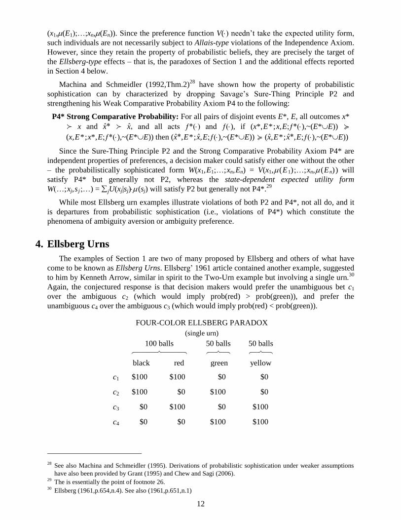
Again, the conjectured response is that decision makers would prefer the unambiguous bet c1
over the ambiguous c2 (which would imply prob(red) > prob(green)), and prefer the
unambiguous c4 over the ambiguous c3 (which would imply prob(red) < prob(green)).
FOUR-COLOR ELLSBERG PARADOX
(single urn)
100 balls 50 balls 50 balls
black red green yellow
c1 $100 $100 $0 $0
c2 $100 $0 $100 $0
c3 $0 $100 $0 $100
c4 $0 $0 $100 $100
28 See also Machina and Schmeidler (1995). Derivations of probabilistic sophistication under weaker assumptions
have also been provided by Grant (1995) and Chew and Sagi (2006). 29
The is essentially the point of footnote 26. 30
Ellsberg (1961,p.654,n.4). See also (1961,p.651,n.1)
13
4.1 Initial Reactions and Discussion
Because they struck at the heart of what many considered to be basic principles of rationality
– the Sure-Thing Principle and probabilistic beliefs – Ellsberg’s examples spawned a lot of
discussion among the decision theory establishment. Ellsberg summarized some of their initial
reactions as follows:31
“Responses do vary. There are those who do not violate the axioms, or say they won’t, even
in these situations (e.g., G. Debreu, R. Schlaifer, P. Samuelson); such subjects tend to apply
the axioms rather than their intuition, and when in doubt, to apply some form of the Principle
of Insufficient Reason. Some violate the axioms cheerfully, even with gusto (J. Marschak, N.
Dalky); others sadly but persistently…. Still others (H. Raiffa) tend, intuitively, to violate the
axioms but feel guilty about it and go back into further analysis.”
Ellsberg’s report of a wide range of views on these issues played out in the subsequent
literature. Whether or not he had any intuitive tendency for violation, Raiffa (1961) offered what
has come to be the standard argument to an individual who would make the typical choices in the
Three-Color Urn: If you really prefer a1 over a2 and a4 over a3, then you presumably prefer a
50:50 coin flip of a1:a4 versus a 50:50 coin flip of a2:a3. But both coin flips reduce to a purely
objective 50:50 coin flip of $100:$0. In Raiffa’s view, “Something must give!” (1961,p.694)
Others have expressed a variety of views. Although Fellner (1961) largely supported a
decision maker’s right to possess Ellsberg-like preferences, he also asked whether a decision
maker “is or is not likely gradually to lose this trait as he gets used to the uncertainty with which
he is faced.”32
Brewer (1963) argued that the rationality/irrationality of Ellsberg-type “slanting
down of subjective probabilities” depends on whether or not a decision maker is allowed a free
choice to bet on either an event or its complement – if not, he argues, Raiffa’s comparison with a
50:50 coin flip won’t apply (discussion of these issues continued in Fellner (1963) and Brewer
and Fellner (1965)). Roberts (1963) reported, but did not accept, the argument that losing in
either bet b2 or bet b4 on the 50:50 urn is somehow different from losing in either bet b1 or bet b3
on the unknown urn.33
Smith (1969) and Sarin and Winkler (1992), however, suggest that a
decision maker indeed does have distinct (and measurable) utility of money functions for prizes
won from the two different urns. Finally, historians of economic thought are directed to the
interesting 1961-1963 correspondence between Ellsberg and Leonard Savage (Savage (1963)).
4.2 Experiments on Ellsberg Urns and Ambiguity Aversion
Although Ellsberg himself only offered his examples as thought experiments, he recognized
the need for formal experimentation from the very start.34
The earliest reported experiments of
this form seem to be those of Chipman (1958,1960).35
Fellner (1961) offered various versions of
the Two-Urn problem to a group of Yale undergraduates, and found an overall tendency to prefer
the 50:50 rather than the unknown odds. Subsequent experiments by Becker and Brownson
(1964), MacCrimmon (1968), Slovic and Tversky (1974), Curley and Yates (1989) and others
also confirmed Ellsberg’s conjecture of widespread ambiguity aversion. Although most of these
experiments use students as subjects, researchers such as MacCrimmon (1965), Hogarth and
31 Ellsberg (1961,pp.655-656).
32 Fellner (1961,pp.678-679), original emphasis.
33 “If I pick [bet b1], I would be completely out of luck if there were no red balls in the urn.” (p.333). See also the
discussion of Roberts (1963) and Ellsberg (1963) on Roberts’ notion of “vagueness” in decision making and its
implications for Ellsberg-type choice situations. 34
“To test the predictive effectiveness of the axioms … controlled experimentation is in order.” (1961,p.655,n.6). 35
See footnote 2 above.
14
Kunreuther (1989), Einhorn and Hogarth (1986), Viscusi and Chesson (1999), Ho, Keller and
Keltyka (2002) and Maffioletti and Santori (2005) have examined the ambiguity preferences of
business owners, trade union leaders, actuaries, managers and executives, with the same overall
findings.
In their own series of experiments, MacCrimmon and Larsson (1979) recognized that the
interesting parameter in Ellsberg’s examples was not the winning prize level, but rather, the
amount of objective versus subjective uncertainty, which in the Three-Outcome Urn is given by
the (known) proportion of red balls in the urn. MacCrimmon and Larsson’s sequence of
experiments accordingly set out to examine how subjects’ choices depended on this proportion.
In the standard specification of the Three-Color Urn, the proportion of red balls is ⅓ (30 out of
90). Of course, if the proportion of red balls were actually zero, all subjects would prefer option
a2 in the first pair and a4 in the second pair, which is consistent with the Sure-Thing Principle,
and if this proportion were unity, all would now prefer a1 in the first pair and a3 in the second
(also consistent with the Sure-Thing Principle). As the proportion increased from zero toward
unity, the percentage of a1 choices and a3 choices should both rise, and under the hypothesis of
ambiguity aversion, there would be some intermediate interval of probabilities within which a
subject’s choice would have flipped from a2 to a1, but not yet flipped from a4 to a3 yielding the
classic Ellsberg-type violation of the Sure-Thing Principle for this urn. Using 100-ball urns,
MacCrimmon and Larsson were able to present subjects with urns whose red-ball proportions
took the values 0.20, 0.25, 0.30, 0.33, 0.34, 0.40, and 0.50. They indeed found such an
intermediate interval of probabilities, and perhaps not surprisingly, the percentage of such
violations was the greatest at p = .33.
Although each of Ellsberg’s own examples pits a purely objective urn against an ambiguous
urn with a fixed probability range,36
researchers have also explored attitudes toward changes in
the size of this range (holding the center constant). Becker and Brownson (1964), Larson (1980)
and Viscusi and Magat (1992) did find an aversion to increases in the size of the range; Curley
and Yates (1985) and Yates and Zukowski (1976) did not. In a reversal of Ellsberg’s original
specification of a fixed prize and ambiguous probability, Eliaz and Ortolevaz (2011) also found
ambiguity aversion in the case of a fixed objective probability but an ambiguous prize level.37
Du
and Budescu (2005) found that subjects were willing to pay more to reduce the range
(“vagueness”) of outcome uncertainty than probability uncertainty.38
While the phenomena of Reduction of Compound Lotteries and ambiguity neutrality are
distinct properties, many researchers consider them to be closely related, and some of the
rationality arguments against ambiguity aversion (such as Raiffa’s (1961)) explicitly or
implicitly invoke the reduction principle. In an experimental examination of this, Halevy (2007)
appended two urns to the original two-color urns: one urn where the proportion of black balls
satisfied a uniform objective distribution, and one urn which was either all black, or all red, with
objective 50:50 probabilities. The two urns, together with Ellsberg’s Urn I, are all purely
objective, and each reduces to a 50:50 objective lottery over the best:worst monetary prize.39
However, in Halevy’s second urn all uncertainty is resolved in the first stage, whereas in
Ellsberg’s urn I all uncertainty is resolved in the second stage (Halevy’s first urn involves both
first stage and second stage uncertainty). Using this framework, Halevy found that subjects who
36 In the Three-Color Paradox the unknown probability of a black ball ranges from 0 to ⅔; in the Two-Urn Paradox
it ranges from 0 to 1; in the Four-Color Paradox it ranges from 0 to ½. 37
See these authors’ further results in the case of joint outcome/probability ambiguity. 38
Outcome and probability ranges were each classified into “low,” “medium,” or “high” levels of vagueness. 39
Halevy used the prizes $2:$0 and $20:$0 for both his own and those of Ellsberg’s urns used in his experiments.
15
satisfied the Reduction of Compound Lotteries Axiom under objective uncertainty were typically
ambiguity neutral. Ozdenoren and Peck (2008) also took a dynamic approach, framing a two-
stage Ellsberg urn problem as a “game against nature” and exploring various implications for
ambiguity aversion and dynamic consistency.
Another systematic feature of attitudes toward ambiguity – reported in Ellsberg (1962,2001)
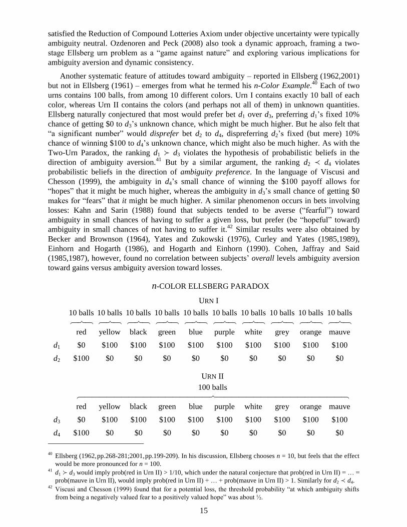
but not in Ellsberg (1961) – emerges from what he termed his n-Color Example.40
Each of two
urns contains 100 balls, from among 10 different colors. Urn I contains exactly 10 ball of each
color, whereas Urn II contains the colors (and perhaps not all of them) in unknown quantities.
Ellsberg naturally conjectured that most would prefer bet d1 over d3, preferring d1’s fixed 10%
chance of getting $0 to d3’s unknown chance, which might be much higher. But he also felt that
“a significant number” would disprefer bet d2 to d4, dispreferring d2’s fixed (but mere) 10%
chance of winning $100 to d4’s unknown chance, which might also be much higher. As with the
Two-Urn Paradox, the ranking d1 d3 violates the hypothesis of probabilistic beliefs in the
direction of ambiguity aversion.41
But by a similar argument, the ranking d2 d4 violates
probabilistic beliefs in the direction of ambiguity preference. In the language of Viscusi and
Chesson (1999), the ambiguity in d4’s small chance of winning the $100 payoff allows for
“hopes” that it might be much higher, whereas the ambiguity in d3’s small chance of getting $0
makes for “fears” that it might be much higher. A similar phenomenon occurs in bets involving
losses: Kahn and Sarin (1988) found that subjects tended to be averse (“fearful”) toward
ambiguity in small chances of having to suffer a given loss, but prefer (be “hopeful” toward)
ambiguity in small chances of not having to suffer it.42
Similar results were also obtained by
Becker and Brownson (1964), Yates and Zukowski (1976), Curley and Yates (1985,1989),
Einhorn and Hogarth (1986), and Hogarth and Einhorn (1990). Cohen, Jaffray and Said
(1985,1987), however, found no correlation between subjects’ overall levels ambiguity aversion
toward gains versus ambiguity aversion toward losses.
n-COLOR ELLSBERG PARADOX
URN I
10 balls 10 balls 10 balls 10 balls 10 balls 10 balls 10 balls 10 balls 10 balls 10 balls
red yellow black green blue purple white grey orange mauve
d1 $0 $100 $100 $100 $100 $100 $100 $100 $100 $100
d2 $100 $0 $0 $0 $0 $0 $0 $0 $0 $0
URN II
100 balls
red yellow black green blue purple white grey orange mauve
d3 $0 $100 $100 $100 $100 $100 $100 $100 $100 $100
d4 $100 $0 $0 $0 $0 $0 $0 $0 $0 $0
40 Ellsberg (1962,pp.268-281;2001,pp.199-209). In his discussion, Ellsberg chooses n = 10, but feels that the effect
would be more pronounced for n = 100. 41
d1 d3 would imply prob(red in Urn II) > 1/10, which under the natural conjecture that prob(red in Urn II) = … =
prob(mauve in Urn II), would imply prob(red in Urn II) + … + prob(mauve in Urn II) > 1. Similarly for d2 d4. 42
Viscusi and Chesson (1999) found that for a potential loss, the threshold probability “at which ambiguity shifts
from being a negatively valued fear to a positively valued hope” was about ½.
16
Forms of Preference Elicitation
One methodological issue, present throughout experimental work on choice and decision
making, concerns exactly how preferences over Ellsberg-type prospects “should” be elicited.
Ellsberg’s original presentations, and the great preponderance of subsequent experiments, simply
presented subjects with pairs of alternative, and asked for a direct choice within each pair. But
standard consumer theory posits that the same ranking would be revealed if a subject’s
preferences were instead assessed via an independent monetary valuation of each prospect,43
with the valuations then compared. Fox and Tversky (1995), Chow and Sarin (2001) and Du and
Budescu (2005) and found that ambiguity aversion was reduced substantially (though not
completely) when subjects were asked for separate monetary evaluations of ambiguous and
unambiguous prospects (via their willingness to pay or willingness to accept) rather than asked
for direct comparisons.
In another alternative to simple pairwise choice, MacCrimmon and Larsson (1979) presented
subjects with sets of 11 prospects each, and asked them for a complete ranking of all prospects
within each set (indifference was allowed). By including bets on stock index prices along with
classic Ellsberg urns in their menus, these researchers were able to explore another question
related to ambiguity, namely how subjects treated ambiguity in unknown urns with ambiguity
outside of the laboratory.44
MacCrimmon and Larsson found no net effect in either direction.
Experimental Studies of Insurance and Medical Decisions Under Ambiguity
Other experimenters have also elicited subjects’ ambiguity preferences in choices more
relevant and realistic than simply drawing balls from urns. An obvious domain is that of
insurance. Experiments on insurance decisions under ambiguity typically place subjects in the
role of either consumers or suppliers of contracts such as flood or earthquake insurance, product
warranties, etc. Although subjects are typically students, experiments and surveys by Einhorn
and Hogarth (1986), Hogarth and Kunreuther (1992), Kunreuther (1989) and others have also
found ambiguity aversion in hypothetical decisions by both professional actuaries and
experienced insurance underwriters. Kunreuther, Meszaros, Hogarth and Spranca (1995) found
ambiguity aversion in a field survey of primary-insurance underwriters in commercial property
and casualty insurance companies. In experiments which included professional actuaries, and
where subjects were asked to price insurance both as consumers and firms, Hogarth and
Kunreuther (1989) found results which paralleled those of Kahn and Sarin (1988), Viscusi and
Chesson (1999) and others as reported above, namely that both consumers and firms revealed
ambiguity aversion toward low likelihood losses, which decreased as the likelihood of the loss
increased. In an experiment involving real losses, Koch and Shunk (2013) found that ambiguity
aversion was higher under unlimited liability than limited liability. Market and policy
implication of ambiguity aversion are examined in Hogarth (1989), Camerer and Kunreuther
(1989a,1989b), Hogarth and Kunreuther (1985) and Kunreuther and Hogarth (1992). Baillon,
Cabantous and Wakker (2012) explore how different ambiguity attitudes play out in group belief
aggregation.
Medical decisions by both patients and doctors, which also inherently involve ambiguity,
have also been proposed to experimental subjects. Such experiments include decisions regarding
vaccination of children (Ritov and Baron (1990)), heart disease (Curley, Young and Yates
(1989)), residential location based on health risks (Viscusi, Magat and Huber (1991), Viscusi and
43 Such as the procedure of Becker, DeGroot and Marschak (1964).
44 Selten has suggested that many subjects may feel they can make “a very good estimate” of stock market events,
and suggests investment in developing counties as better for such experiments (MacCrimmon (1968,p.28)).
17
Magat (1992)) and others (e.g., Curley, Eraker and Yates (1984)). Gerrity, Devellis and Earp
(1990) developed a multivariate measure of physicians’ reactions to uncertainty, and used the
results of an extensive survey to develop two “reliable and readily interpretable subscales” which
they term “stress from uncertainty” and “reluctance to disclose uncertainty to others.”
Additional Experiments on Ambiguity and Ambiguity Aversion
In other experiments involving real-world scenarios, Hogarth (1989) and Willham and
Christensen-Szalanski (1993) gave subjects actual medical liability cases and manipulated
ambiguity about the probability of winning in a legal scenario where hypothetical plaintiffs and
defendants had to decide whether to go to court or settle out of court. In direct comparisons
across contexts, Kahn and Sarin (1988) found that consumers’ ambiguity attitudes differed
across choices involving radio warranties, pharmaceutical decisions and restaurant food quality.
Maffioletti and Santori (2005) examined subjects’ attitudes toward bets on real-world election
results, and Baillon and Bleichrodt (2011) used bets on the temperature and on stock index
prices. And while initially solely the realm of economists and psychologists, experimental work
on decisions under ambiguity has now extended to the realm of neurology.45
Ambiguity aversion has been and continues to be one of the most intensively experimentally
explore phenomena in decision theory. Further discussion of this literature is provided in the
surveys listed in Section 8.
5. Models and Definitions of Ambiguity Aversion
Unlike the economic concepts of “risk” and “risk aversion,”46
there is not unanimous
agreement on what “ambiguity aversion,” or even “ambiguity” itself, exactly is. However several
models and definitions have been proposed.
Most (though not all) of these models take as their starting point the following formalization
of the objective/subjective uncertainty framework of Sections 3.1 and 3.4. Preferences are
defined over the domain of horse-roulette acts – henceforth called acts – namely maps ƒ = (…;Pj
if Ej;…) = (…;(…;xij,pij ;…),Ej ;…) from a (finite or infinite) state space S to roulette lotteries Pj
over a set of prizes X. The Independence property over this richer domain is identical to the
Independence Axiom of objective expected utility, except for the more general notion of
probability mixing it entails. Probability mixtures of horse-roulette acts are defined statewise:
given acts ƒ = (…;Pj if Ej;…) and g = (…;Qj if Ej;…) over a common47
partition {E1,…,En} of
the state space S, and probability (0,1), the mixture ƒ + (1–)g is defined as the act
ƒ + (1–)g = (…;Pj + (1–)Qj;…)
The axioms that characterize subjective expected utility in this framework are accordingly48
Weak Order: is complete and transitive
Non-Degeneracy: There exist acts ƒ and g for which ƒ g
Continuity: For all acts ƒ,g,h, if ƒ g and g h, there exist , (0,1) such that
ƒ + (1–)h g and g ƒ + (1– )h
45 See Hsu, Bhatt, Adolphs, Tranel and Camerer (2005), Chew, Li, Chark and Zhong (2008), Huettel, Stowe,
Gordon, Warner and Platt (2006), as well as the survey of Weber and Johnson (2008). 46
E.g., Rothschild and Stiglitz (1970), Pratt (1964). 47
As before, {E1,…,En} could be any common refinement of the two acts’ original partitions. 48
These versions of the expected utility axioms, due to Fishburn (1970), are referred to in the literature as the
Anscombe-Aumann axioms. See also Schmeidler (1989).
18
Independence: For all acts ƒ,g,h and all α (0,1), ƒ g if and only if ƒ + (1–)h
g + (1–)h
Monotonicity: For all acts ƒ,g, if the roulette lottery ƒ(s) is weakly preferred to the roulette
lottery g(s) for every state s, then ƒ g
The expected utility representation of preferences over horse-roulette acts ƒ = (…;Pj if Ej;…)
= (…;(…;xij,pij ;…),Ej ;…) implied by these axioms takes the form
1 1(ƒ) (ƒ( )) ( ) ( ) ( ) ( ) ( )
n n
j j ij ij jjS j iW U s dµ s U µ E U x p µ EP
where U() is a von Neumann-Morgenstern utility function and µ is a finitely additive probability
measure (“prior”), which is uniquely identified as in Savage’s axiomatization. As seen in the
above equation, the term U(ƒ(s)) in the integral SU(ƒ(s))d(s) is the expected utility of the
roulette lottery ƒ(s). This is also the case for many of the models that we consider in this section,
and that are axiomatized in the horse-roulette framework.
The above Independence axiom49
turns out to imply the Sure-Thing Principle,50
which
implies that any Ellsberg-type violation of the Sure-Thing Principle is also a violation of
Independence. It follows that any model of ambiguity aversion in the horse-roulette act
framework must relax Independence.
Versions of the above axioms can also be stated in a setting closer to that of Savage, where
acts are purely subjective horse lotteries. This requires that the set of prizes be suitably rich (for
instance, an interval of the real line), with a suitable notion of “subjective mixture” on prizes.
Nakamura (1990), Gul (1992) and Wakker (1989) take this approach, and Ghirardato,
Maccheroni, Marinacci, and Siniscalchi (2003) introduce a general notion of subjective mixture
of prizes which allows a direct translation of the above axioms, and many of their relaxations are
discussed in this section.
5.1 Maxmin Expected Utility / Expected Utility with Multiple-Priors
Gilboa and Schmeidler (1989,p.142) suggest the following explanation of the modal behavior
in the Ellsberg Paradox:
“One conceivable explanation of this phenomenon which we adopt here is as follows:
[…] the subject has too little information to form a prior. Hence (s)he considers a set of
priors as possible. Being uncertainty averse, (s)he takes into account the minimal
expected utility (over all priors in the set) while evaluating a bet.” (original emphasis)
The resulting model is called Maxmin Expected Utility (MEU) or sometimes the Multiple-
Priors (MP) model.51
Formally, consider a closed,52
convex set C of probability measures –
49 We distinguish between the two identically named conditions by the capitalization “Independence Axiom” for the
Marschak/Samuelson axiom of Section 3.2 and “Independence axiom” for the current Independence property. 50
Defining event mixtures as in Section 3.1, suppose (ƒ*,E ; ƒ ,~E) (ƒ,E ; ƒ ,~E). By Independence,
½(ƒ*,E ; ƒ ,~E) + ½(ƒ*,E ; ƒ ,~E) ½(ƒ,E ; ƒ ,~E) + ½(ƒ*,E ; ƒ ,~E), which can be equivalently written as
½(ƒ*,E ; ƒ ,~E) + ½(ƒ*,E ; ƒ ,~E) ½(ƒ,E ; ƒ ,~E) + ½(ƒ*,E ; ƒ ,~E). Invoking Independence once again yields
(ƒ*,E ; ƒ ,~E) (ƒ,E ; ƒ ,~E). 51
The expression “multiple-priors” is potentially ambiguous, because there are several well-known models which
also employ sets of priors (for instance, Variational and Smooth Ambiguity Preferences models). 52
If the state space is finite, the set C is closed in the usual Euclidean topology. If it is infinite, it is closed in the
weak* topology.

19
priors – on the state space S, and a von Neumann-Morgenstern utility function U(⋅). An act ƒ(⋅) is evaluated according to
minƒ( ) ƒ( )C
W U d
(1)
To see how this model allows for the typical preferences in Ellsberg’s examples, consider the
Three-Color Paradox of Section 1 (the analysis of the Two-Urn Paradox is similar). Let the state
space be S = {sr,sb,sy}, where sr denotes the draw of a red ball, etc., let the set of prizes be X =
{$0,$100}, and set U($100)= 1 and U($0) = 0. To reflect the assumption that 30 out of the 90
balls in the urn are red, but that the number of black and yellow balls is not known, consider the
set of priors53
C = {(S):(sr)} = ⅓ (2)
Under this set of priors, the four acts in the Three-Color Paradox are evaluated as
W(a1) = ⅓ W(a2) = 0 W(a3) = ⅓ W(a4) = ⅔
which implies the Ellsberg rankings a1 a2 and a3 ≺ a4.54
To derive these values, observe that
every prior C assigns probability ⅓ to the state sr, so that W(a1) = ⅓. Similarly, every prior
C assigns probability ⅔ to the event {sb,sy}, so that W(a4) = ⅔. Act a2 yields $100 on state sb
and $0 otherwise; in other words, it is a bet on black. The prior in C that assigns zero probability
to sb is the one that minimizes expected utility, and will accordingly be the one selected by the
MEU criterion, so that W(a2) = 0. In other words, the individual evaluates a bet on black as if
none of the 60 unknown balls in the urn were black. Act a3 yields $100 on the event {sr,sy} and
zero otherwise; in other words, it is a bet against black. This time, the prior in C that assigns unit
probability to sb (thus zero probability to sy) is the one that minimizes expected utility and hence
is the one selected, so that W(a3) = ⅓. That is, the individual evaluates a bet against black as if
all of the 60 unknown balls were black. This is a (stark) example of the “worst-case scenario”
thinking embodied in equation (1). While the set C used here is extreme, it is not the only one
that generates the standard Ellsberg preferences: any set of priors where the probability of sr is
constant at ⅓ and the probability of sb ranges from less than ⅓ to greater than ⅓ will yield the
above rankings.
As a historical note, Ellsberg himself proposed a decision criterion that is effectively a
special case of MEU. He proposes that, by careful deliberation, an individual faced with an
ambiguous situation may nevertheless “arrive at a composite ‘estimated’ distribution 0 that
represents all his available information on relative likelihoods”; however, due to ambiguity,
“[o]ut of the set (S) of possible distributions there remains a set 𝒟 of distributions that still
seem ‘reasonable,’ reflecting judgments that he ‘might almost as well’ have made, or that his
information… does not permit him confidently to rule out.”55
He then suggested (p.664) that
individuals may evaluate acts according to the criterion
0minƒ( ) ƒ( ) (1 ) ƒ( )
DW U d U d
where ρ represents the individual’s “degree of confidence” in the estimate 0, and C =
0 + (1–)𝒟 is seen to be the set of priors. Kopylov (2006) analyzes this model when the set
𝒟 equals the set (S) of all possible probability distributions – a specification which also appears
in the literature on robust Bayesian analysis.
53 () denotes the family of probability measures over a set. To simplify notation, we write ({sr}), ({sr,sb}),
v({sr}),… as (sr), (sr,sb), v(sr),… for measure (and later capacity) values over singletons or finite sets. 54
Note this also implies that a3 is considered no better than a1, in spite of the fact that it yield a higher payoff on sy. 55
Ellsberg (1961,p.661); notation in this paragraph adapted to the present chapter.
20
Gilboa and Schmeidler (1989) axiomatize the MEU decision criterion via axioms on horse-
roulette acts. They retain the Weak Order, Monotonicity, Continuity and Non-Degeneracy
axioms stated above, but weaken Independence, replacing it with
Certainty Independence: For all acts ƒ,g, all constant acts x, and all (0,1): ƒ g if
and only if ƒ + (1–)x g + (1–)x
Uncertainty Aversion: For all acts ƒ, g and all (0,1): ƒ g implies ƒ + (1–)g g
That Independence must be relaxed follows from the fact that, as noted above, Independence
implies Savage’s Postulate P2, and hence must be violated by Ellsberg-type preferences. The key
question is to what extent Independence should be weakened. To gain some intuition, it is useful
to add to the four acts a1,…,a4 of the Three-Color Paradox a fifth act a5 representing a bet on
yellow: specifically, a5 yields $100 if a yellow ball is drawn and $0 otherwise. An individual
with MEU preferences characterized by the set C in equation (2) will be indifferent between
betting o29n black or on yellow, that is, a2 ~ a5. However the mixture ½a2 + ½a5 is strictly
preferred to a2, which would not be possible with EU preferences. How should it be interpreted,
and what is its relationship to ambiguity?
Act a2 will yield $100 if the ambiguous color black is drawn and $0 if the ambiguous color
yellow is drawn. Act a5 instead yields $100 if yellow and $0 if black. Thus, whether or not the
better prize $100 is obtained – if it is obtained at all – hinges crucially on which of the two
ambiguous colors is drawn. (Both acts yield $0 under the unambiguous color red.) By way of
contrast, a 50:50 mixture of the two acts provides hedging: it removes the dependence of the
prize on which of the two ambiguous colors is drawn. Specifically, the mixture ½a2 + ½a5
yields the same objective roulette lottery ($100,½;$0,½) for both of the ambiguous colors yellow
and black. The Uncertainty Aversion Axiom thus reflects a preference for hedging.56
Mathematically, Uncertainty Aversion corresponds to quasiconcavity of the functional
representation of preferences – an analytically convenient property.
On the other hand, mixing an act with a constant act (a constant prize or a constant objective
lottery) does not provide such hedging, and there is less of an argument that such mixtures
should necessarily be preferred (or dispreferred) by an ambiguity averter. The Certainty
Independence Axiom accordingly requires that mixtures with constant acts do not affect
preferences. While MEU preferences do satisfy Certainty Independence, there are reasons to
relax or drop this axiom: see Sections 5.6-5.9.
Gilboa and Schmeidler (1989) show that the above axioms are necessary and sufficient for
the existence of the MEU representation (1), with affine utility function U() and convex set of
priors C which is “identified up to convex closure” – that is, any other set of priors which
represents preferences will have C as its convex closure (the closure of its convex hull).
A generalization of the MEU model is the so-called -maxmin, or -MEU model
min maxƒ( ) ƒ( ) (1 ) ƒ( )C C
W U d U d
(3)
For = 1, this representation reduces to MEU, and for = 0 it reduces to what is termed
maxmax expected utility max CU(ƒ(s))d, and it allows for a whole range of intermediate
attitudes toward ambiguity. Unfortunately, a general, behavioral characterization of this class of
56 The condition “ƒ g implies ƒ ƒ + (1–)g,” known as the Uncertainty Appeal condition, captures the
opposite intuition, and corresponds to the maxmax preference function defined below.
21
preferences is not available.57
Furthermore, the intuitive interpretation of as an ambiguity-
aversion parameter is not warranted in general: Siniscalchi (2006) demonstrates that an -MEU
decision maker with = ⅔ and set of priors specified in (2) will have preferences in the Three-
Color problem that are indistinguishable from one with = 1 (i.e., MEU) and set of priors {
(S): (sr) = ⅓, (sb) ≥ 2/9}. The elements and C of the representation are not separately
identified.
Lehrer (2012) axiomatizes a special class of MEU preferences in which the set C is generated
by a partially specified probability. Axiomatizations of MEU which do not rely on horse-roulette
acts, but require a rich outcome space, have been provided by Casadesus-Masanell, Klibanoff
and Ozdenoren (2000a,2000b) and Ghirardato, Maccheroni, Marinacci and Siniscalchi (2003).
5.2 Choquet Expected Utility / Rank-Dependent Expected Utility
Another important model of ambiguity aversion, proposed by Schmeidler (1989), is the
Rank-Dependent or Choquet model. Rather than capturing the individual’s perception of
ambiguity by means of a family of priors as in the MEU model, it does so by means of a single
non-additive probability measure (“capacity”) v(). For example, in the Three-Color problem, the
individual may have the beliefs
ν(sr) = ⅓, ν(sb,sy) = ⅔, ν(sb ) = ν(sy) = (4)
for some [0,⅓). The fact that ν(sb,sy) > ν(sb) + ν(sy) indicates that there is ambiguity about the
relative likelihood of a black vs. yellow draw: there is a residual probability mass equal to
ν(sb,sy) – ν(sb) + ν(sy) that the individual, so to speak, does not know how to allocate between sb
and sy. On the other hand, ν(sb,sy) + ν(sr) = 1 = ν(S), which indicates that there is no ambiguity
about the probability of drawing a red vs. a non-red ball. A non-additive probability measure can
encode both the individual’s assessment of relative likelihoods and the confidence attached to
such assessment in a single function. Formally, a capacity is defined as a non-negative real
function ν(∙) defined over an algebra or -algebra of subsets of the state space S that satisfies the
normalization ν()=0 and ν(S)=1, and the monotonicity property that E F implies v(E) v(F)
(a standard probability measure is a capacity since additivity implies monotonicity). Capacities
need not be additive, but they still retain the property that the weight assigned to a set is not
smaller than the weight assigned to any subset.
Note that given this departure from additivity, specifying the capacity of the individual states
in a finite state space does not fully characterize the capacity. For example, equations (4) do not
pin down a unique capacity, because they leaves ν(sr,sb) and ν(sr,sy) unspecified.
A key issue is how to compute the integral/expected value of a function with respect to a
capacity. Consider a finitely-ranged function g:S → ℝ that takes values 1,…,n. The problem is
that what might seem like the natural definition, namely
( ) ( ) { : ( ) }i ii
g s d s s g s
can lead to failures of monotonicity, even in simple cases.
58
57 Ghirardato, Maccheroni and Marinacci (2004) provide an axiomatization, but it turns out (Eichberger, Grant,
Kelsey and Koshevoy (2011) that their axioms can only hold for the cases = 1 and = 0. Klibanoff, Mukerji
and Seo (2011) provide a non-degenerate axiomatization of -MEU when the state space describes the
realizations of an exchangeable sequence of experiments. 58
For any capacity with ν(sr) = ν(sb) = ν(sy) = ½ and v(sr,sb,sy) = 1, the act {7 if sr ;8 if sb ;9 if sy} will be assigned
the value ½7 + ½8 + ½9 = 12, which exceed the value of 10 assigned to the dominating act {10 if sr ;10 if sb ;10
if sy}. A similar candidate, namely the formula ∑ sg(s)ν(s), is subject to the same difficulties.
22
To resolve this problem, Schmeidler (1986,1989) proposes the use of the Choquet Integral.
Given a function g:S ℝ which takes values 1 > … > n, the Choquet integral of g with
respect to a capacity ν is defined as
1 1 12( ) ({ : ( ) }) { : ( ) } { : ( ) }
n
i i iig s d s g s s g s s g s (5)
The telescoping property of the respective weights
1 1 1({ : ( ) }), , { : ( ) } { : ( ) } , , 1 { : ( ) }
i i ns g s s g s s g s s g s
in this formula ensures that they sum to one, avoiding the difficulties noted in footnote 58. If the
capacity ν is additive, and hence a probability measure, equation (5) reduces to the standard
integral of g with respect to ν. For a general, bounded measurable function g, the Choquet
integral is defined as
0
0{ : ( ) } 1 { : ( ) }g d s g s d s g s d
where the integrals on the right side are in the sense of Riemann
The Choquet Expected Utility (or CEU) representation of preferences over acts ƒ is thus
ƒ( ) ƒ( )W U d (6)
where U(∙) is a von Neumann-Morgenstern utility, ν(∙) is a capacity, and the integral is in the
sense of Choquet. This representation is sometimes also called Rank-Dependent Expected Utility,
with reference to the analogous model of preferences under objective uncertainty.59
To see that the CEU model can accommodate Ellsberg in the Three-Color example, consider
the capacity ν defined by
ν(sr) = ⅓ ν(sb,sy) = ⅔ ν(sb ) = ν(sy) = 1/6 ν(sr,sb) = ν(sr,sy) = ½
and set U($100) = 1 and U($0) = 0. Applying equation (5) yields V(a1) = ⅓, V(a2) = 1/6, V(a3) = ½
and V(a4) = ⅔, giving the Ellsberg rankings a1 a2 and a3 a4.
CEU preferences capture ambiguity aversion (or preference) by allowing the individual to
exhibit a preference (or aversion) for hedging. Observe that a 50:50 probability mixture of the
ambiguous acts b1 and b3 in the Two-Color problem yields the completely objective (and to an
ambiguity averter, strictly preferred) lottery ($100,½;$0,½). This occurs, of course, because b1
yields its best prize $100 for a red draw, whereas b3 yields its best prize for a black draw – the
two acts are, in a sense, “negatively correlated,” so that mixing them in this way reduces the
variability of outcomes (or more generally, utility) across states. Given a pair of multiple-state
acts ƒ = [x1 if s1;…;xn if sn] and g = [y1 if s1;…;yn if sn], this effect will occur, in part, for any a
pair of states si, sj for which xi > xj and yi < yj. When two acts are comonotonic, that is, when xi
xj yi yj for all i, j, probability mixing cannot lead to any hedging.
The Choquet model captures ambiguity aversion/preference by weakening the Sure-Thing
Principle just enough to allow such a preference/aversion for hedging – that is, preferences are
allowed to violate the key mixture property of the axiom so long as, but only so long as, there is
actually some potential for hedging. Whenever there is no such potential, that is, whenever the
acts being mixed are comonotonic, the mixture property must continue to hold:
Comonotonic Independence: For every triple of pairwise comonotonic acts ƒ,g,h, and
every (0,1): ƒ g if and only if ƒ + (1–)h g + (1–)h
59 E.g. Quiggin (1982), Yaari (1987), Segal (1987b). See also Section 5.3 below.
23
Schmeidler (1986) shows that a function defined on simple (or bounded) measurable
functions is monotonic, as well as both monotonic and additive with respect to comonotonic
functions, if and only if it is a Choquet integral. Building on this, Schmeidler (1989) shows that
CEU preferences are characterized by Weak Order, Continuity, Monotonicity, Non-Degeneracy,
and the Comonotonic Independence Axiom. The uniqueness properties of CEU are the same as
those for SEU: the capacity ν is unique, and utility is unique up to a positive affine
transformation.
As noted, CEU preferences needn’t be uncertainty-averse. Schmeidler (1989) demonstrates
that a CEU preference function will satisfy the Uncertainty Aversion Axiom of Section 5.1 if and
only if its capacity ν is convex: that is, if for every pair of events E,F, ν(EF) + ν(EF) ≥ ν(E) +
ν(F). Uncertainty-averse CEU preferences are thus also a (strict) special case of MEU
preferences, where the set C of priors coincides with the core of the capacity ν:
C = core(ν) = { (S):E, (E) ν(E)}
Gilboa (1987) and Sarin and Wakker (1992) provide axiomatizations of CEU in the original
Savage framework. Nakamura (1990) provides another, in a setting where the state space can be
finite, provided the set of prizes is suitably rich. Another axiomatization of CEU in a fully
subjective setting with rich outcomes can be found in Ghirardato, Maccheroni, Marinacci and
Siniscalchi (2003). The most complete exposition of the rank-dependent model is that of Wakker
(2010). Lehrer (2009) proposes an integral for capacities that coincides with the Choquet integral
if the capacity is convex, but is different in general.
5.3 Segal’s Recursive Model
The Recursive Model of Segal (1987a) is the earliest of a group of models which can be
described as “two-stage.” Ambiguity is modeled by assuming that the probability distribution
over the state space S is not known, but random with probability measure M over (S). In the
first stage, one particular probability measure (S) is realized. In the second stage, the state s
is drawn according to the distribution . The first stage may be only an idealization, a fictitious
construct that is helpful to describe a particular way to evaluate acts; the second stage is real.
Here we assume that all measures have finite-support.
Under this model, an individual treats a basic act (…;xj if Ej ;…) as the two-stage prospect
(…;(…;xj ,Ej ;…),k;…), where k, the probability distribution (prior) over states, is the
realization of the first-stage uncertainty, and Ej, the realized event under distribution k, is the
realization of second stage uncertainty.60
Each such act has a corresponding two-stage objective
lottery of the form (…;(…;xj ,k-1
(xj);…),M(k);…). The key question is how to evaluate such
two-stage acts and lotteries.
An individual who applies the Reduction of Compound Lotteries (ROCL) axiom of Section
3.1 to collapse this two-stage objective lottery to a single-stage one cannot exhibit Ellsberg-type
preferences: such an individual will be probabilistically sophisticated, with statewise subjective
probabilities kk(si)M(k). Segal, however, argues that it is appropriate to drop ROCL in such
a setting:
“…if a sufficiently long time passes between the two stages of the lottery, then there is no
reason to make this reduction assumption… It is my belief that decision makers consider
60 Since is involves the orthogonal state spaces S and (S), the mixture (…;(…;xj ,Ej ;…),k;…) is to be
distinguished from a two-stage subjective act (…;ƒj() if Ej;…) as defined in Section 3.1, which involves
subpartitions of (…;{…,Ej k,…};…) of a common state space S.
24
the Ellsberg urn as a real two-stage lottery, in which the first, imaginary stage and the
second, real stage are clearly distinguishable. Therefore, they do not feel themselves
obliged to obey the reduction of compound lotteries axiom…” (1987a,p.178)
Segal begins by assuming the individual has a preference function V(∙) defined over single-
stage lotteries. Given an act ƒ() = (…;xj ,Ej;…), each measure over S induces a simple lottery
of the form (…;xj ,(Ej) ;…) and the individual uses V() to determine the certainty equivalent
CE(ƒ,) of this lottery, that is, the value for which
V(CE(ƒ,),1) = V(…;xj ,(Ej);…)
The individual’s uncertainty over the measure (), as represented by the measure M() over
the space (S), generates the real-valued lottery (…;CE(ƒ,k),M(k);…).61
The individual
evaluates this lottery again using the function V(), which yields the preference function
W(ƒ()) V(…;CE(ƒ,k),M(k);…) (7)
Together, this implies the chain of indifferences
ƒ() (…;ƒ( ),k;…) (…;CE(ƒ( ),k),k ;…) (…;CE(ƒ(),k),M(k);…)
or equivalently
(…;xj ,Ej ;…) (…;(…;xj ,Ej ;…),k;…) (…;CE((…;xj ,Ej ;…),k),k;…)
(…;CE((…;xj ,Ej ;…),k),M(k);…)
where the first object is the subjective act ƒ() from states to payoffs which is being evaluated,
the second is the representation of this act as a map from the set of measures k (S) to
subjective acts which takes the value ƒ() for all k, the third is the map from this set of measures
to the act’s certainty equivalent under each measure, and the fourth is the objective lottery over
these certainty equivalents values implied by the probability measure M() over the measures.
If the preference function V() over objective lotteries is expected utility, then the final
evaluation reduces to subjective expected utility. However, Segal suggests using anticipated
utility, or rank-dependent expected utility form (Quiggin (1982), Yaari (1987), Segal (1987b)).
For a lottery P = (…; i, pi;…), with 1 > … > n, this preference function takes the form
1 1 1 1 12( ) ( ) ( ) ( ) ( ... ) ( ... )i i i
n
iV U p U p p p p
P
As such, it is analogous to the Choquet expected utility form (5) over subjective acts, with the
nonadditive capacity v replaced by a nonlinear (and typically convex) distortion function : [0,1]
→ [0,1] for which (0) = 0 and (1) = 1. When () is linear, this form reduces to objective
expected utility.
Labeling the induced lotteries Pk = (…;xj ,k(Ej);…) so that V(P1) ≥… ≥ V(Pn), and observing
that the certainty equivalent of a lottery P is given by U-1
(V(P)), the Recursive preference
function over subjective acts takes the form
1 1 1 1 12(ƒ( )) ( ) ( ( )) ( ) ({ ,..., }) ({ ,..., })i i i
n
iW V M V M M
P P
To illustrate how this model can accommodate Ellsberg preferences in the Three-Color Urn,
keep the normalization U($100) = 1 and U($0) = 0, and suppose that the decision-maker assigns
probability ½ to each of the distributions
61 For simplicity, we assume that the measure M over (S) has finite support.
25
1 2( , , ) ( , ,0) ( , , ) ( ,0, )r b y r b ys s s s s s ⅓ ⅔ ⅓ ⅔
(8)
Then bet a1 on red induces the same lottery P = {$100,⅓;$0,⅔} under either measure, so we can
identify it with the degenerate two-stage lottery {P,1} to obtain W(a1) = V(P) = (⅓). A similar
argument establishes W(a4) = V(P) = (⅔).
Consider now the bet a2 on black. Under distribution 1 it yields the lottery P1 =
{$100,⅔;$0,⅓}, while under 2 it yields P2 = {$100,0;$0,1}. We have V(P1) = (⅔) and V(P2) =
0, so from equation (7), W(a2) = V(P1)∙ (M(µ1)) = (⅔)∙ (½). A similar argument establishes
W(a3) = 1∙ (½) + (⅓)[1– (½)]. For distortion function (p) = (ep–1)/(e–1) these values
become62
W(a1) = 0.2302 > 0.2082 = W(a2) and W(a3) = 0.5208 < 0.5516 = W(a4), which yield
the Ellsberg rankings.
While Segal (1987a) utilizes the same preference function to evaluate single-stage lotteries as
well as lotteries over certainty equivalents, Segal (1990) considers the possibility of using
different preference functions in the two stages.
5.4 Klibanoff, Marinacci and Mukerji’s Smooth Ambiguity Preferences
Model
The Smooth Ambiguity Preferences Model Klibanoff, Marinacci and Mukerji (2005) (KMM)
follows a similar two-stage approach. The main differences with Segal’s Recursive Model are
that the primitives are preferences over horse lotteries, i.e., subjective acts, rather than objective
roulette lotteries, and that different preference functions are used in the different stages. In
particular, these are each expected utility functions, with different utility functions. This is
related to Example 2 in Segal (1990).
In applications, the smooth representation typically takes the following form: for any act
(horse lottery) ƒ : S→ X, the smooth ambiguity index is
( )
ƒ( ) ƒ( ) ( )W U d dM
S (9)
where U(∙) is the von Neumann-Morgenstern utility function, M is the individual’s second-order
prior, that is, a probability measure over the set (S) of measures μ on the state space S, and φ(∙) is the individual’s second-order utility function. As in Segal’s Recursive model, the
interpretation is that the individual is uncertain about which probability measure μ describes the
likelihood of realizations of the state; this second-order uncertainty is modeled using the second-
order prior M. Each measure μ determines a different expected utility ∫U(ƒ())dμ for the act f. If
the individual simply averaged these expected utilities using M, and hence evaluated f according
to
( )
ƒ( ) ( )U d dM
S S
this would yield expected utility preferences, where the subjective probability measure is the
“average measure” that assigns to each event E the probability ∫μ(E)dM(μ). Instead, the
individual “distorts” the expected utilities ∫U(ƒ())dμ using the second-order utility function φ(∙). As we shall see momentarily, concavity of φ(∙) corresponds to a notion of ambiguity aversion.
(Similarly, convexity of φ(∙)corresponds to ambiguity preference, and linearity of φ(∙) corresponds to expected utility and hence ambiguity neutrality).
To see how this representation can accommodate the modal preferences in the Three-Color
Paradox, suppose that, as in the preceding subsection, the individual assigns equal second-order
62 Segal (1987a,p.185), see also his Theorem 4.2 for a general result along the lines of this example.
26
probabilities to the distributions in equation (8). Continue to assume that U($100) = 1 and U($0)
= 0, and let φ(r) = √–r. Then W(a1) = φ(⅓) = 0.5773 > 0.4082 = ½φ(⅓) + ½φ(0) = W(a2) and
similarly W(a3) = ½φ(⅓) + ½φ(1) = 0.7887 < 0.8165 = φ(⅔) = W(a4), as required.
We now show how KMM obtain the representation in equation (9); in so doing, we also
illustrate the formal connection with Segal’s approach.
KMM adopt a decision framework in which, loosely speaking, the realizations of objective
roulette wheels are modeled as part of the state space; preferences over acts that depend only on
the roulette-wheel component of the state space are assumed consistent with EU with a uniform
prior probability measure. Formally, the state space S is the Cartesian product of a set Ω of
interest and the interval [0,1] (the roulette wheel). The set of prizes is an interval of real numbers.
The individual is endowed with not one, but two preference relations. The first, denoted , is a
preference over (standard) acts ƒ:S→ X. Its restriction to the set of acts that only depend on the
roulette-wheel component [0,1] of the state space S is assumed to admit an expected utility
representation, with a continuous, strictly increasing utility U and a prior which is the
Lebesgue measure on [0,1]. It is clear that, for every roulette lottery P = (…;xi ,pi;…) with prizes
in the set X, there exists an act ƒP that depends only on the roulette-wheel component of the state
space and which generates the same probability distribution as P, in the sense that ({r:ƒP(ω,r) =
xi for all ω}) = pi for all i. For this reason, call such acts lottery acts.
The second preference relation, denoted (2)
, is defined over second-order acts, i.e., maps
ƒ(2)
:(S) → X. We return to the interpretation of this relation below. The relation (2)
is
assumed to have an expected utility representation, with continuous, strictly increasing utility v
(not necessarily equal to U) and probability measure M ((S)).
The key axiom, Consistency, connects the preferences on standard acts and (2)
on
second-order acts. It also indicates how the Smooth Ambiguity Preferences model is related to
Segal’s Recursive approach. The Consistency axiom formalizes Segal’s analysis of the Three-
Color Urn in the previous subsection (and is also consistent with Segal’s own intended use of the
model). We assumed that each act a1,a2,a3,a4 was associated with a collection of single-stage
lotteries, corresponding to the probability distributions over states that the individual
contemplates; then, we evaluated the act by evaluating the two-stage lottery obtained by
attaching probabilities to each such single-stage lottery. KMM’s Consistency axiom makes this
process explicit: they associate with each standard act ƒ the second-order act ƒ(2)
such that, for
every (S), ƒ(2)
() is a certainty equivalent of the lottery act that yields each outcome x in
the range of ƒ with probability measure (ƒ-1
(x)). Given the assumption that preferences over
lottery acts are consistent with expected utility, with a continuous and strictly increasing (hence,
invertible) utility function U(), this means that
(2) 1ƒ ( ) ƒ( )U U d
for every (S). The key assumption is then
Consistency: For all acts ƒ,g, ƒ g iff ƒ(2)
(2)
g(2)
That is: the ranking of f and g is precisely the ranking of the corresponding second-order acts ƒ(2)
and g(2)
.
Consistency and the assumption that preferences over second-order acts admit an expected
utility representation then immediately imply that standard, first-order acts ƒ can be ranked
according to
(2)
( ) ( )ƒ( ) ƒ ( ) ( ) ƒ( ) ( )W v dM U d dM
S S
27
where φ(∙) = v(U-1
(∙)) is the second-order utility and M the second-order probability measure, or
second-order prior. This is the representation in equation (9). (In KMM, each measure in the
support of the second-order prior is an independent product of Lebesgue measure on [0,1] and
a suitable probability measure on the coordinate of actual interest, namely . In applications, the
Lebesgue component is simply omitted.) Notice that, while this model is commonly referred to
as the Smooth Ambiguity Preferences model, the function φ is not necessarily smooth (though it
can be, and typically is, in applications).
The interpretation of second-order acts requires some elaboration. KMM acknowledge that a
direct interpretation of them as bets on different elements in (S) is not straightforward:
“there is a question whether preferences with respect to these acts are observable. The
mapping from observable events to events in (S) may not always be evident. When it is
not evident we may need something richer than behavioral data, perhaps cognitive data
or thought experiments” (p. 1854).
If second-order acts are not directly observable, then the second-order utility v and second-
order probability measure M should be thought of solely as a way to provide a numerical
representation of preferences over first-order, standard acts. The question is then whether these
objects can be identified on the basis of preferences over standard acts alone. In general, the
answer is negative: for a trivial example, observe that, if the second-order utility () is linear
(equivalently, if v = U), one can equivalently replace a given second-order probability measure
M with one that is concentrated on the “average probability measure” ∫ dM() without
changing first-order preferences at all. As KMM indicate, it is an open question to what extent
and under what conditions () and M can be identified from first-order preferences alone. For an
environment in which uncertainty concerns infinitely many repetitions of an experiment, a
positive answer is provided by Klibanoff, Mukerji and Seo (2011) under a “symmetry”
restriction on preferences. A related result can be found in Al-Najjar and De Castro (2013).
On the other hand, there are settings in which second-order acts are observable. An obvious
example are experiments involving physical devices: one can resolve bets on the composition of
an urn by simply opening the urn and examining its contents. Bets on long-run averages can also
be thought of as observable second-order acts, though arguably only as idealizations or
approximations. However, in these cases, first- and second-order acts only differ because they
depend on different “coordinates” of the state space; the model in equation (9) essentially allows
the individual to be differently risk-averse, depending on the source of uncertainty. In other
words, rather than ambiguity attitudes, the smooth model reflects issue preference, which we
consider in the following section.
An alternative axiomatization of the Smooth Ambiguity Preferences model is provided by
Seo (2009). That paper takes a different approach. The individual is assumed to have preferences
over roulette-horse-roulette acts (see Section 3.4). The key assumption is that individuals do not
reduce compound lotteries, though they satisfy a suitable “dominance” property. Seo obtains an
extension of the representation in equation (9) to lotteries over horse-roulette acts; the function
() captures both attitudes towards ambiguity and violations of reduction. Thus, one implication
of his model is that an agent who reduces compound objective lotteries must be ambiguity-
neutral. There is some evidence that attitudes toward reduction and ambiguity are correlated
(Halevy (2007)); however, one may wish for a model that does not impose perfect correlation
between these distinct behavioral traits.
The main attraction of the Smooth Ambiguity Preferences model is its tractability. The
numerical example above suggests that calculations may involve simple adaptations of familiar
28
expected utility analysis. As further evidence, KMM show that concavity of the second-order
utility function () corresponds to a notion of “ambiguity aversion” which implies Schmeidler’s
Uncertainty Aversion Axiom (although their notion is defined in terms of second-order beliefs,
and hence subject to the preceding qualifications).
5.5 Ergin and Gul’s Issue-Preference Model
Ergin and Gul (2009) propose a variant of Segal’s two-stage approach, and provide an
elegant axiomatization in a Savage-style environment. Their model highlights a different
interpretation of the Ellsberg Paradoxes.
To illustrate, it is useful to rephrase the Three-Color Paradox slightly. Imagine that the balls
in the urn are numbered from 1 to 90. Balls numbered 1–30 are known to be red. Balls numbered
31–90 may be either black or yellow: the color of each of these balls is not known. Thus, the
experiment involves two sources of uncertainty, or issues: the number of the ball drawn, and the
colors of balls 31–90. Importantly, these issues are independent: if you learn the number of the
ball drawn, that does not tell you anything about the colors of balls 31–90, or conversely.
This richer description can be modeled using a two-coordinate state space, for example
S = {1,…,90} {c = (c31,…,c90) : i, ci {b,y}}
Denote an arbitrary state in S by s = (n,c), where n is the number of the drawn ball and c is a
color assignment, i.e., vector (c31, …, c90). The bets in the Three-Color Paradox can then be
modeled as follows (with some abuse of notation, we use the same letters as in Section 1): the
bets on “red” and “black or yellow” correspond respectively to
1 4
$100 1,...,30 $0 1,...,30( , ) and ( , )
$0 31 $100 31
n na n c a n c
n n
The bets on “black” and “red or yellow,” on the other hand, correspond to
2 3
$0 1,...,30 $100 1,...,30
( , ) $100 31and and ( , ) $0 31and
$0 31and $100 31and
n n
n n
n n
a n c n c b a n c n c b
n c y n c y
An obvious difference between a1 and a4 on one hand, and a2 and a3 on the other, is that the
former only depend upon the number of the ball drawn, whereas the latter depend upon both the
number of the ball drawn and the color assignment to balls 31…90 (in particular, the color of the
ball drawn). Now suppose that the individual has probabilistic beliefs, and in particular believes
that every ball is equally likely to be drawn, and also that, independently, every color assignment
is equally likely to have occurred. This implies that, for both acts a1 and a2, the probability of
receiving $100 is ⅓; similarly, the probability of winning is ⅔ for both acts a3 and a4. The
Ellsberg preferences a1 a2 and a3 ≺ a4 can then interpreted as follows: despite the fact that the
winning probabilities in each comparison are the same, the individual prefers bets that only
depend upon the first issue (here, the number of the ball drawn) to bets that depend upon both
issues (the number as well as the color assignment).
Recall that an individual is probabilistically sophisticated if he or she evaluates an act ƒ =
(…;xj ,Ej ;…) by first reducing it to a lottery Pƒ = (…;xj ,(Ej);…) where is their subjective
probability over the state space S, and then applying a suitable preference function over lotteries.
Even in the above modified formulation of the Three-Color Urn bets, Ellsberg preferences are
not probabilistically sophisticated – acts that induce the same probability distribution over prizes

29
are strictly ranked. However, Ergin and Gul note that they are second-order probabilistically
sophisticated, in the sense that each act is evaluated by first reducing it to a compound lottery, in
which the first stage corresponds to the assignment of colors to balls 31,…,90 and the second
stage corresponds to the draw of a numbered ball from the urn, and then applying a suitable
compound-lottery preference function. This reduction of acts to compound lottery is essentially
what was done in order to apply Segal’s two-stage model to the Three-Color Paradox. Ergin and
Gul point out that this form of reduction is a higher-order version of probabilistic sophistication
and, more importantly, provide a complete axiomatization of the resulting preferences.
Their axiomatization builds upon that of Machina and Schmeidler (1992) for probabilistically
sophisticated preferences in a Savage framework (Section 3). To provide some detail, assume
that the state space is a Cartesian product, S = Sa × Sb, where the two coordinates correspond to
issue a and issue b. In the Three-Color Urn, issue a is the number of the ball drawn, and issue b
is the color assignment. The Machina-Schmeidler Strong Comparative Probability axiom is
applied only to acts that depend solely on issue a. Ergin and Gul’s key novel axiom, a|b Strong
Comparative Probability, serves three purposes. First, it implies that Strong Comparative
Probability also holds for acts that depend solely on issue b. Second, it implies that the two
issues are statistically independent, as in the example. Third, it implies, loosely speaking, that the
individual is concerned with second-order risk related to issue b, and not second-order risk
related to issue a (Ergin-Gul (2009,p.906) provide an illustration).
To formally describe the Ergin-Gul representation, note that exploiting the product structure
of the state space allows an act ƒ to be represented as
11 1 1
1
1
ƒ
m
n nm n
m
x x A
x x A
B B
where {A1,…,An} is a partition of Sa, {B1, …, Bm} is a partition of Sb, and xij is the prize
delivered by ƒ at all states s Ai × Bj. Given a product measure = a × b on S, associate with
ƒ the two-stage compound lottery
ƒ* ...; ...; , ( ) , ( );...i j a j b jx A B P
Under Ergin and Gul’s axioms, there exists a unique product measure = a × b on S such
that every act ƒ is evaluated according to W(ƒ(∙)) = V*(Pƒ*), where Pƒ* is the compound lottery
associated with ƒ and V* is a suitably continuous preference function on two-stage lotteries that
satisfies stochastic dominance; again, see the original paper for details. If a version of Savage’s
Sure-Thing Principle is imposed, this function reduces to two-stage expected utility with
different utility functions, as in the Smooth Ambiguity Preferences model of Section 5.3. If
instead a Comonotonic Sure-Thing Principle axiom is imposed, the first-stage lottery is
evaluated using a Choquet integral. Ergin and Gul also draw a formal connection between
uncertainty aversion and issue preference.
Nau (2006) proposes a related model, which allows for state-dependent preferences but
restricts attention to additive representations in both stages. Different perspectives on source
preference are suggested by Chew and Sagi (2008) and Abdellaoui, Baillon, Placido and Wakker
(2011). Finally, Skiadas (2013) assumes that prizes are monetary and preferences over acts are
scale-invariant: (…; xj,Ej;…) (…; yj,Fj;…) if and only if, for every real number > 0,
30
(…;xj,Ej;…) (…;yj,Fj;…). This yields a two-stage expected utility representation a la
Ergin and Gul, with different constant relative risk averse utility functions for the two stages.
5.6 Vector Expected Utility
Siniscalchi (2009a) proposes a different approach to modeling ambiguity-sensitive
preferences. There are three key ingredients in this approach. First, the individual evaluates acts
by a process reminiscent of “anchoring and adjustment” (Tversky and Kahneman (1974)).
Second, the anchor is a standard expected utility evaluation, where expectations are taken with
respect to a baseline subjective probability measure. Third, the adjustment depends upon a
measure of statistical similarity of the act under consideration with “examples” or “models” of
ambiguous acts.
The proposed representation is called vector expected utility (VEU) because a key role is
played by a vector of expectations. Specifically, the VEU representation evaluates acts according
to
1ƒ( ) ƒ( ) ƒ( ) , ,..., ƒ( ) , nW U d A cov U cov U (10)
where is the baseline prior, ζ1,…,ζn are adjustment factors, i.e., real-valued functions on the
state space S that satisfy ∫ ζi d = 0, cov(∙,∙) denotes covariance (computed with respect to ), and
A(∙) is the adjustment function, which satisfies A(0,…,0) = 0 and A(φ) = A(–φ) for every vector φ.
Notice that, due to the normalization of the adjustment factors ζ1,…,ζn,
ƒ( ) , ƒ( )i icov U U d
To see how the VEU model accommodates Ellsberg preferences, consider a simple
specification with a single adjustment factor ζ1, defined by
1(sr) = 0 1(sb) = 1 1(sy) = –1
a uniform baseline prior, and the adjustment function
A(φ) = – |φ |
The adjustment factor ζ1 can be interpreted as a bet whereby the individual wins or loses one
util, depending on which of the two ambiguous colors is drawn, but nothing happens if the
unambiguous color red is drawn. 63
Intuitively, this suggests that ζ1 is a “purely ambiguous” bet,
and indeed a model of the kind of bets that are ambiguous in this problem.64
A related interpretation of the adjustment factor ζ1 formalizes the following intuition,
proposed by Epstein and Zhang (2001) for the modal preferences in the Ellsberg Paradox:
“The intuition for this reversal is the complementarity between sb and sy – there is
imprecision regarding the likelihood of sb, whereas {sb, sg} has precise probability ⅔” (p.
271; italics added for emphasis, and notation adapted to this chapter).
The fact that ζ1(sb) = 1 whereas ζ1(sr) = 0 reflects the perception that sb is ambiguous but sr is
not; setting ζ1(sy) = –1 indicates that ambiguity about sb and sy “cancels out.” In this sense, sb and
sy are complementary in the VEU representation; this formalizes the Epstein-Zhang
interpretation. (The relationship with the previous interpretation is that, in order for ζ1 to be a
purely ambiguous bet in this example, it must reflect the complementarity between sb and sy).
63 For the sake of this interpretation, assume that initial utility is constant and normalized to zero.
64 This intuitive interpretation corresponds closely to the way adjustment factors are formally identified from
preferences: see Section 4.1 in Siniscalchi (2009a).
31
We now verify that the VEU representation proposed here induces the Ellsberg rankings.
1
2
3
4
1 13 3
1 133
2 1 13 33
2 23 3
( ) | 0 |
( ) | | 0
( ) | |
( ) | 0 |
W a
W a
W a
W a
In the calculation of W(a4), the covariance term is zero precisely because ambiguity about sb and
sy cancels out: cov(U(a4)), ζ1) = ⅓∑s ζ1(s)a4(s) = ⅓(0∙0 + 1∙1 + 1∙(–1)) = 0.
The key axiom in the characterization of VEU preferences is Complementary Independence.
A preliminary definition: two acts ƒ,ƒc are complementary if the mixture ½ƒ + ½ƒ
c is a constant
act. Intuitively, complementary acts are the “negative” of each other, up to a constant. An
important feature is that they share the same prize variability, or volatility: if the (utility of the)
prizes delivered by ƒ at different states varies a lot, the same is true of prizes delivered by ƒc,
except that prizes vary in opposite directions. The main axiom for VEU preferences is then
Complementary Independence: For all acts ƒ,g,ƒc,g
c such that ƒ,ƒ
c and respectively g,g
c
are complementary: if ƒ ƒc and g g
c, then ½ƒ + ½g ½ƒ
c + ½g
c
When comparing complementary acts, variability cannot play a role because, as just noted,
any two complementary acts have the same volatility. The axiom requires that, absent volatility
considerations, a form of Independence must hold. This implies that any departures from
expected utility must be determined by attitudes toward variability. For further interpretation, the
reader is referred to the original paper.
VEU preferences can accommodate a wide range of ambiguity attitudes. If the Uncertainty
Aversion Axiom is imposed, the function A must be negative and concave. It turns out that a
negative, but not necessarily concave function A also captures a notion of ambiguity aversion;
we discuss this further in Section 6.
Chambers, Grant, Polak and Quiggin (2013) consider preferences that admit a representation
similar to that of equation (10), but with an arbitrary aggregator to combine the baseline
expectation and adjustment terms. They adopt the Complementary Independence axiom, and also
require a form of uncertainty aversion. See also Grant and Polak (2013).
5.7 Variational and Multiplier Preferences
The Uncertainty Aversion Axiom of Section 5.1 is common to a broad class of preference
models. In addition to MEU preferences, suitable parameterizations of smooth ambiguity, Ergin-
Gul, and VEU preferences also satisfy it. As we will discuss in Section 6, its interpretation is not
entirely straightforward, or uncontroversial; on the other hand, the fact that it is a familiar and
analytically convenient quasiconcavity assumption has made it an obvious reference point in the
theoretical and applied literature on ambiguity-sensitive preferences. This subsection and the
next two discuss other preference models that satisfy Uncertainty Aversion, and can be thought
of as direct generalizations of the MEU specification.
To introduce these models, recall that the characterization of MEU preferences also involves
Certainty Independence. Unlike the Uncertainty Aversion Axiom, Certainty Independence is
seen to be quite restrictive. We noted in Section 5.1 that, when an act such as a2 (bet on black) in
the Three-Color-Urn is mixed with a constant act, no hedging occurs: like the act a2, the mixture
yields a strictly better prize in case a black ball is drawn than if a yellow or red ball is drawn. By
way of contrast, mixing a2 with a bet on yellow results in an act which delivers a good prize if
32
either of the ambiguous colors is drawn. However, mixing a2 with a constant act does have two
potentially important effects. First, it reduces the utility variability across the two ambiguous
states sb and sy: for instance, a2 yields utility U($100) and U($0) in case a black or, respectively,
non-black ball is drawn, whereas a 50:50 mixture of a2 with the constant act $0 yields ½U($100)
+ ½U($0) and U($0) respectively. Second, mixing with a constant act also shifts utilities up or
down: to see this, compare the utilities delivered by a 50:50 mixture of a2 with $0 to those
delivered by a 50:50 mixture of a2 with $100, namely U($100) for a black ball and ½U($100) +
½U($0) for a non-black ball.
Both of these changes may potentially affect preferences. After all, in choice under risk,
changes in the scale (i.e., outcome variability) and location (upward/downward shifts) of
monetary prizes can affect preferences. For instance, if preferences exhibit decreasing absolute
risk aversion, an individual becomes more willing to take bets as their initial (nonrandom) wealth
increases, i.e., shifts upward. Similarly, unless preferences are homothetic, an individual with
constant initial wealth may accept a given bet, but turn it down if both their wealth and the stakes
in the bet are doubled (or vice versa). Arguably, it would be desirable to allow for similar
behavior in the context of ambiguity: changing the scale and/or location of utilities may
influence preferences. However, Certainty Independence is a location- and scale-invariance
assumption, so such phenomena are ruled out.
Variational Preferences
Motivated in part by these considerations, Maccheroni, Marinacci and Rustichini (2006a)
propose a weakening of Certainty Independence:
Weak Certainty Independence: For all acts ƒ,g, constant acts x,y and all (0,1): if
ƒ + (1–)x g + (1–)x, then ƒ + (1–)y g + (1–)y
This axiom assumes invariance to changes in the location, but not the scale, of utilities. In the
Three-Color Urn problem, it allows for the following pattern of preferences:
a1 a2 and ½a1 + ½0 ½a2 + ½0
A possible interpretation might be that, by scaling down the utilities of the acts involved in
the comparison, the individual becomes less sensitive to the fact that black is an ambiguous color
but red is not. (We do not claim that such preferences would be reasonable or natural, merely
that they are allowed by Weak Certainty Independence.) At the same time, Maccheroni et al.’s
axiom still requires that, since the 50:50 mixture of a1 with $0 is considered worse than the 50:50
mixture of a2 with $0, the same must be true if $0 is replaced with $100.
Maccheroni et al. show that the Weak Order, Non-Degeneracy, Monotonicity, Continuity,
Uncertainty Aversion and Weak Certainty Independence Axioms are necessary and sufficient for
the existence of a representation of the form
( )
minƒ( ) ƒ( ) ( )W U d c
S (11)
where c : (S) → [0,∞] is a lower semicontinuous, convex cost function that satisfies inf c() =
0. They call equation (11) the variational representation of preferences.
The cost function c(∙) is the key ingredient of the representation. Once a utility function has
been fixed, a “canonical” or “minimal” cost function is uniquely identified (refer to Maccheroni
et al. for details). If the utility function U is replaced with a positive affine transformation U +
, the cost function c must be replaced with c.
33
Observe that the minimization in equation (11) is over all priors over the state space S.
However, one can obtain MEU preferences as a special case as follows: fix a compact, convex
set C of priors, and define
0( )c
C
C
(such a function is often called an “indicator function” in convex analysis). With this
specification of the cost function, it is clear that a prior C will never be a solution of the
minimization problem in equation (11) whereas priors in C are costless, so the minimization
problem reduces to that in equation (1).
Maccheroni et al. propose the following “malevolent Nature” interpretation. When the
individual contemplates choosing an act ƒ, Nature tries to minimize its expected utility. To do so,
she can choose any prior (S); however, to choose , Nature must pay a cost c(). In the
case of MEU preferences, priors in C are costless, and all other priors are infinitely costly;
however, the variational representation allows for intermediate cases as well – that is, for priors
that have a nonzero but finite cost. Nature’s problem is thus to minimize the sum of the
individual’s expected utility and the cost of priors.
Skiadas (2013) also axiomatizes a version of Variational Preferences with constant relative
risk averse utility.
Multiplier Preferences
Another special parameterization of Variational Preferences deserves special mention.
Hansen and Sargent (2001) and Hansen, Sargent and Tallarini (1999) consider the following
specification:
( )
ƒ( ) min ƒ( ) ( || *)W U d R
S (12)
where attention is restricted to countably additive probability measures when the state space is
infinite, θ ≥ 0 is a parameter, and R( || *) denotes the relative entropy of the prior with
respect to a reference prior *. The latter is defined as
*
|| * logd
dR d
if is absolutely continuous with respect to *, and R( ||
*) = ∞ otherwise. This defines the
so-called Multiplier Preferences preference function. Equation (12) is a special case of equation
(11), yielding tractability since the explicit solution to the problem in equation (12) is known,
and indeed one can show that
ƒ( )
ƒ( ) log exp *U
W d
(the reason for the two consecutive minus signs will be clear momentarily). An exact
characterization of Multiplier Preferences within the class of Variational Preferences is provided
by Strzalecki (2011).
The above equation indicates that, if one restricts attention to horse lotteries, i.e. acts that
map states to prizes (rather than to roulette lotteries over prizes), Multiplier Preferences are
ordinally equivalent to SEU preferences with utility function –exp(–θ-1U(∙)). To see this, note
that W(ƒ(∙)) is the composition of the function ∫-exp(–θ-1U(∙)) d, which takes on strictly
negative values, with the function x –θ log(–x), which is strictly increasing when restricted to
34
the negative reals. On the other hand, if one restricts attention to roulette lotteries, the
individual’s risk preferences are represented by U(∙). In other words, one can interpret the
multiplier-preferences model as postulating that the individual is more risk-averse toward
subjective risk than toward objective risk. The idea that risk attitudes may be source-dependent
was discussed in Section 5.5.
5.8 Confidence-Function Preferences
Chateauneuf and Faro (2009) propose a model that is “dual” to Variational Preferences:
whereas the latter relax the scale-invariance requirement of Certainty Independence but preserve
location-invariance, Chateauneuf and Faro’s Confidence-Function Preferences retain scale
invariance but drop translation invariance. More precisely, these authors assume that the set X of
prizes contains a worst element x*, and impose
Worst Independence: For all acts ƒ,g and all (0,1): ƒ ~ g implies ƒ + (1–)x* ~
g + (1–)x*
Together with Weak Order, Continuity, Monotonicity, Ambiguity Aversion and other
axioms, Worst Independence characterizes the following representation:
: ( )
1
( )ƒ( ) min ƒ( )W U d
(13)
where the utility function U(∙) satisfies U(x*) = 0, is a parameter in (0,1], and φ(∙) is an upper
semicontinuous, quasiconcave function on (S) that satisfies φ() = 1 for some prior .
The proposed interpretation is that φ(∙) measures the “degree of confidence” that the
individual assigns to the different measures. Nature is malevolent, and wants to minimize the
individual’s expected utility. However, she must choose only priors to which the individual
assigns a high enough level of confidence. Furthermore, Nature must pay a multiplicative cost
φ()-1
to choose the prior .
Confidence-function preferences are positively homogeneous: if all utility values are
multiplied by some constant > 0, the function in equation (13) is also multiplied by . If utility
is also positively homogeneous, i.e., if it displays constant relative risk aversion, then the overall
representation of preferences is also positively homogeneous. This is convenient in certain
applications, especially in financial economics. Furthermore, it makes it possible to invoke
standard results on the existence of a representative agent.
5.9 Uncertainty-Averse Preferences
Cerreia-Vioglio, Maccheroni, Marinacci, and Montrucchio (2011) characterize the class of
preferences that satisfy Continuity, Monotonicity and Uncertainty Aversion, in addition to
Independence on lotteries and certain other technical assumptions. In other words, they drop both
location and scale invariance. Their powerful result unifies all the models that generalize MEU,
as well as many other specifications, such as the Smooth Ambiguity Preferences model. The
general Uncertainty-Averse Preferences representation is
( )
ƒ( ) min ƒ( ) ,W G U d
S (14)
where the function G : ℝ × (S) → (–∞, +∞] is quasiconvex, increasing in the first variable, and
satisfies inf(S)G(t,) = t for all t.
35
Due to their generality, Uncertainty-Averse Preferences representations are only unique in a
weak sense. For a fixed utility function, there is a minimal function G(∙,∙). If a positive affine
transformation of U is taken, G must be suitably rescaled.
MEU preferences are, of course, also Uncertainty-Averse Preferences, with
( , )t
G t
C
C
Variational Preferences correspond to the special case
G(t,) = t + c()
whereas Confidence-Function Preferences obtain if
( )( )( , )
( )
t
G t
Finally, recall that Smooth Ambiguity Preferences also satisfy Uncertainty Aversion,
provided the second-order utility function φ(∙) is concave. Under additional technical
assumptions, Cerreia-Vioglio et al. show that the Smooth Ambiguity Preference representation
can be written as in equation (14), with
( )
min( , ) |tM
G t t I M M
where is the second-order probability measure in the Smooth Ambiguity Preferences
representation, Γ() is the set of second-order measures N ((S)) that reduce to , in the
sense that
( )( ) ( ) ( )E dM E
S
for every event E S, and It(M|) is a so-called statistical distance function, i.e., a non-
negative, lower semicontinous, quasiconvex function that satisfies It( | =0 (a specific
formula is provided by Cerreia-Vioglio et al.). In other words, Nature attempts to minimize the
expected utility of the act under consideration by choosing a probability distribution , at a cost
given by the result of the minimization problem above. The latter has an interesting “prior
uncertainty” interpretation: out of all second-order probability measures whose reduction
equals , Nature chooses the one closest to. As for Multiplier Preferences, the intuition is that,
while is the individual’s “preferred” second-order belief, measures close to it are also
plausible.
5.10 Gul and Pesendorfer’s Expected Uncertain Utility
Gul and Pesendorfer (2013) introduce a new model that can accommodate Ellsberg
preferences, as well as source preference. Their model applies to a setting a la Savage, with an
infinite state space S and outcomes in some real interval [l,m]. The key intuition is that the
individual is able to assign probabilities to a (suitably rich) collection of events, but displays
complete ignorance with respect to all other events.
Formally, the proposed representation, Expected Uncertain Utility (EUU) starts with a -
algebra Σ, which comprises the events whose likelihood the individual can confidently assess. A
countably additive and non-atomic measure represents beliefs on Σ. The EUU model ranks Σ-
measurable acts according to expected utility; these acts are “unambiguous.” The question is how
36
to rank an arbitrary Savage act ƒ:S→[l,m] that is not Σ-measurable. To do so, according to EUU,
the individual brackets any act ƒ between a lower Σ-measurable approximation ƒ1 and an upper
Σ-measurable approximation ƒ2, in the sense that
({s:ƒ1(s) ƒ(s) ƒ2(s)}) = 1
and furthermore such pair (ƒ1,ƒ2) is the “tightest” approximation of ƒ: if there is another pair
(g1,g2) with the same property, then ({s : g1(s) ≤ ƒ1(s) ≤ ƒ2(s) ≤ g2(s)}) = 1. The last ingredient
of the EUU representation is a continuous, increasing interval utility function, that is, a map
U(,) from the set I = {(x,y) : x ≤ y} to ℝ. The interpretation is that U(x,y) is the utility of
receiving a prize somewhere in the interval [x,y], when the individual is completely ignorant as
to which prize in this interval he or she will actually receive. The representing function is then
1 2ƒ( ) ƒ ( ), ƒ ( )W U d (15)
To see how this representation works, consider a bet on an event A, i.e., an act ƒ = (x,A;
y,~A) with x > y (which implies that x is strictly preferred to y). If the event A is not in Σ, the
measure does not assign a probability to it; however, we can consider the quantity sup {(E) :
E Σ, E A}. There will be an event E1 Σ that attains this supremum. Similarly, there is an
event E2 Σ that attains sup {(E) : E Σ, E ~ A}. A bracketing of the binary act ƒ is then
given by ƒ1 = (x, E1; y, ~E1) and ƒ2(x, ~E2; y, E2). Then
W(ƒ()) = U(x,x) (E1) + U(y,y) (E2) + U(y,x) (~(E1E2))
This has an intuitive interpretation. On the unambiguous event E1 A, the individual
receives x for sure. Similarly, he or she receives y on E2 ~A. How about states that belong to
neither E1 nor E2? Some of these states are in A, and some are in ~A, but the individual is unable
to rank the relative likelihood of A\E1 and (~A)\E2. Thus, according to EUU, he or she assigns to
all such states the interval utility value U(y,x) – by definition, the utility assigned to receiving
some prize between y and x.
The authors provide an elegant, Savage-style axiomatization of EUU. The events in Σ are
identified as those events for which Savage’s Sure-Thing Principle P2 holds, provided it holds
for their complement as well. An axiom in the spirit of Savage’s P6 ensure the existence of a rich
collection of such events. Furthermore, a rich collection of events similar to ~(E1E2) in the
above example is also assumed. The reader is referred to the original paper for further details.
5.11 Bewley’s Incomplete-Preference Model
A common feature of all the preceding models is that, despite the presence of ambiguity, the
individual was assumed to be able to rank all acts, or all suitably measurable acts. Bewley
(2002,2011) proposes a different approach: he assumes that, due to ambiguity, some acts may
simply not be comparable. For example, Bewley’s take on the Three-Color Paradox is that, quite
simply, the individual is unable to compare a bet on red to a bet on black, or a bet on red or
yellow to a bet on black or yellow.
He proposes a representation of incomplete preferences that features a set C of probability
distributions, as in MEU. According to his model, for any two acts ƒ,g, ƒ is preferred to g if and
only if
ƒ( ) ( )U d U g d C
37
This is sometimes called the unanimity rule: all priors in C must “agree” that ƒ is better than g.
This representation plays a role in recent developments on the definition of ambiguous beliefs, as
in Section 6.
To complement this incomplete decision criterion, Bewley suggests an inertia assumption,
which is essentially a form of status-quo bias: if an act ƒ describes the individual’s initial
endowment, or default option, and there is no act g that is strictly better than ƒ according to the
above criterion, the individual retains ƒ.
The connection between inertia and the status-quo bias is formalized in Ortoleva (2010). This
paper takes as primitive a collection of preferences over acts, of which one is an “unconditional”
preference, and the others are preferences “conditional” upon an exogenously given status-quo
act. Under suitable axioms, the joint representation of these preferences identifies an underlying
incomplete, Bewley-style preference, and involves inertia.
5.12 Models with “Objective Ambiguity”
Ambiguity and ambiguity attitudes have also been modeled by extending von Neumann and
Morgenstern’s analysis of expected utility under objective uncertainty rather than Savage’s
axiomatization of expected utility under subjective uncertainty.
One approach in this strand of the literature identifies ambiguous bets and acts with sets of
lotteries. For instance, a bet on the ambiguous color black in the Three-Color Paradox can be
identified with the set {P = ($100,;$0,1–): [0, ⅔]}. An unambiguous act such as a bet on
red is instead identified with the singleton set {($100,⅓;$0,⅔)}. These sets of lotteries are not
part of a parametric representation: in this model, they are the objects of choice. A state space is
not specified. The individual is characterized by a preference ordering over sets of objective
lotteries. Preferences over singleton sets obey the von Neumann-Morgenstern axioms; the
interest is chiefly in the way non-singleton sets are evaluated.
Olszewski (2007) characterizes the -MEU criterion, with strictly between 0 and 1. Ahn
(2008) proposes the criterion
( )( )
( )
PU dV A
A
where is a measure over all lotteries that is “conditioned” on each menu A, U is a von
Neumann-Morgenstern utility, and φ is an increasing function. Dumav and Stinchcombe (2013)
provide a general analysis of linear representations of preferences over sets of lotteries, and
investigate the connection with models that do employ a state space, such as the ones described
in Sections 5.1-5.11.
A related literature considers preferences over tuples consisting of a set of probability
distributions on a state space, an act, and possibly a reference probability. Sets of probability
distributions can be interpreted as representing imprecise information, perhaps obtained by
econometric techniques. The issue of interest is how to model the individual’s attitudes toward
such imprecise information.
Gajdos, Hayashi, Tallon and Vergnaud (2008) consider preferences over pairs (P,ƒ) of
probability sets and acts (note that it is assumed that comparisons with different sets of
probability distributions are also observed). A first, general representation evaluates such a pair
by a maxmin criterion applied to a suitably selected subset of P. Under additional assumption, an
elegant representation is obtained for finite state spaces, in which (P,ƒ) is evaluated according to
a weighted average of the minimum expected utility over P and the expected utility with respect
38
to the Steiner point of P (a construct which generalizes the notion of center of gravity). Wang
(2003) instead considers preferences over tuples (P,p,ƒ), where P is a set of probability
distributions, p is a reference prior (a distinguished element of P) and ƒ is an act. He axiomatizes
a MEU criterion in this set, as well as an analog of the Multiplier Preferences representation of
Hansen and Sargent (2001).
Viscusi (1989) proposes a different approach within the von Neumann-Morgenstern
framework, termed Prospective Reference Theory. He suggests that “stated” probabilities in a
lottery are not necessarily taken at face value by the individual. Rather, they are interpreted as
signals about the “true” probabilities. Individuals then behaves according to a weighted average
of the stated probability and a prior, or baseline, probability; importantly, they may attribute
different weights to the stated probabilities of different events. In particular, they may assign
greater weight to the stated probability of a red draw from the Three-Color Ellsberg urn than to
the stated probability of a black draw; correspondingly, they may assign a greater weight to the
stated probability of a yellow or black draw than to the stated probability of a red or black draw.
This allows the Prospective Reference Theory model to match the modal preferences in the
Three-Color Paradox.
6. Recent Definitions and Examples
6.1 Recent Definitions of Ambiguity and Ambiguous Events
The parametric representations of preferences discussed in Section 5 suggest conditions
under which an event E may be deemed “ambiguous.” For instance:
The intuitive interpretation of the Maxmin Expected Utility model is that the individual
may be unable to assign a unique probability to certain events; thus, an event E may be
called “ambiguous” if minC (E) < maxC (E).
A similar interpretation applies to the Smooth Ambiguity Preferences model: E is
ambiguous if minsupp M (E) < maxsupp M (E), where M is the second-order prior and
“supp” denotes the support of a measure.
The suggested interpretation of the Choquet Expected Utility model is that the individual
expresses his or her lack of confidence in likelihood assessments by violating additivity.
Thus, E may be called “ambiguous” if the capacity v satisfies v(E) + v(~E) < 1.
In the Vector Expected Utility model, the adjustment function captures departures from
expected utility, so E may be called “ambiguous” if A(cov(1E ,ζ1),…,cov(1E ,ζn)) ≠ 0.
However, these definitions are all closely tied to specific functional forms. Several authors have
proposed definitions of ambiguous and unambiguous events that are stated solely in terms of a
decision-maker’s preferences. We now review two that are, in a sense, polar opposites.
The Epstein-Zhang (2001) Definition
Epstein and Zhang (2001) propose a definition of ambiguous and unambiguous events that
generalizes the preference pattern in the Three-Color Paradox. Recall that, loosely speaking, the
modal preferences in that paradox exhibit a kind of preference reversal: the individual prefers to
bet on red rather than on black, but once yellow is added to the event on which the favorable
prize $100 is delivered, the decision-maker prefers to bet on black or yellow rather than on red or
yellow. As noted in Section 5.2, this indicates that there is a “complementarity” between yellow
and black, but not between red and black. The basic idea behind the approach is to take the fact
that yellow is “complementary” to another color (in this case, black) as the defining feature of an
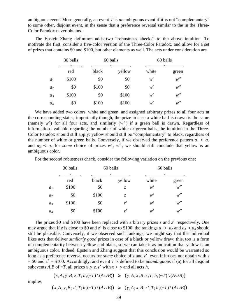
39
ambiguous event. More generally, an event T is unambiguous event if it is not “complementary”
to some other, disjoint event, in the sense that a preference reversal similar to the in the Three-
Color Paradox never obtains.
The Epstein-Zhang definition adds two “robustness checks” to the above intuition. To
motivate the first, consider a five-color version of the Three-Color Paradox, and allow for a set
of prizes that contains $0 and $100, but other elements as well. The acts under consideration are
30 balls 60 balls 60 balls
red black yellow white green
a1 $100 $0 $0 w' w
a2 $0 $100 $0 w' w
a3 $100 $0 $100 w' w
a4 $0 $100 $100 w' w
We have added two colors, white and green, and assigned arbitrary prizes to all four acts at
the corresponding states; importantly though, the prize in case a white ball is drawn is the same
(namely w) for all four acts, and similarly (w) if a green ball is drawn. Regardless of
information available regarding the number of white or green balls, the intuition in the Three-
Color Paradox should still apply: yellow should still be “complementary” to black, regardless of
the number of white or green balls. Conversely, if we observed the preference pattern a1 a2
and a3 ≺ a4 for some choice of prizes w, w, we should still conclude that yellow is an
ambiguous color.
For the second robustness check, consider the following variation on the previous one:
30 balls 60 balls 60 balls
red black yellow white green
a1 $100 $0 z w' w
a2 $0 $100 z w' w
a3 $100 $0 z' w' w
a4 $0 $100 z' w' w
The prizes $0 and $100 have been replaced with arbitrary prizes z and z respectively. One
may argue that if z is close to $0 and z is close to $100, the rankings a1 a2 and a3 ≺ a4 should
still be plausible. Conversely, if we observed such rankings, we might say that the individual
likes acts that deliver similarly good prizes in case of a black or yellow draw: this, too is a form
of complementarity between yellow and black, so we can take it as indication that yellow is an
ambiguous color. Indeed, Epstein and Zhang suggest that this conclusion would be warranted so
long as a preference reversal occurs for some choice of z and z, even if it does not obtain with z
= $0 and z = $100. Accordingly, and event T is defined to be unambiguous if (a) for all disjoint
subevents A,B of ~T, all prizes x,y,z,z with x y and all acts h,
(x ,A; y ,B; z ,T ; h , (~T) \ (AB)) (y ,A; x ,B; z ,T ; h ,(~T) \ (AB))
implies
(x ,A; y ,B; z,T ; h ,(~T) \ (AB)) (y ,A; x ,B ; z,T ; h ,(~T) \ (AB))
40
and furthermore (b) the same is true if T is replaced everywhere with ~T. An event is ambiguous
if it is not unambiguous.
Epstein and Zhang observe that, in general, the collection of unambiguous events is not an
algebra. In particular, the intersection of two unambiguous events may be ambiguous. Zhang
(2000) proposes the following examples: an urn contains white, red, green and blue balls. It is
known that there are 50 red and blue balls, and 50 green and blue balls; the total number of balls
is 100. Intuitively, the events “red or blue” and “green or blue” are unambiguous, but their
intersection, “blue,” is ambiguous.65
However, under suitable assumptions (see below), the
collection of unambiguous events contains the state space S and is closed under complements
and countable disjoint unions; in other words, it is a -system.
Epstein and Zhang consider preferences over Savage acts, and assume that preferences
satisfy Savage’s postulate P3 (Monotonicity). They then consider the family of unambiguous
acts, that is, acts measurable with respect to unambiguous events, and show that, under suitable
axioms, there exists a unique, convex-ranged and countably additive probability measure such
that preferences over unambiguous acts are probabilistically sophisticated with respect to .
The interpretation is as follows: Recall that the Ellsberg Paradoxes contradict not just
expected utility theory, but the more general assumption of probabilistic sophistication.
Conversely, a probabilistically sophisticated individual does not exhibit Ellsberg preferences.
Since the definition of unambiguous events was motivated by analogy with the Three-Color
Paradox, it is almost a tautology that preferences over acts measurable with respect to
unambiguous events cannot exhibit Ellsberg-type behavior. But the Epstein-Zhang result says
much more: preferences over such acts uniquely pin down a probability measure over
unambiguous events, and indeed they are probabilistically sophisticated.
If the decision-maker is probabilistically sophisticated in the sense of Machina and
Schmeidler (1992), then the above definition deems all events to be unambiguous, and the
Epstein-Zhang axioms hold; thus, their result is consistent with Machina and Schmeidler’s. The
Epstein-Zhang result is mainly of interest when the overall preferences are not probabilistically
sophisticated; in such cases, it identifies a subset of events and preferences for which
probabilistic sophistication holds.
Underlying the terminology employed by Epstein and Zhang is the implicit assumption that
ambiguity means a violation of probabilistic sophistication. As we shall see, the approach we
discuss next makes a different implicit assumption.
The Ghirardato-Maccheroni-Marinacci /Nehring Definition
An alternative approach has been suggested by Ghirardato, Maccheroni and Marinacci
(2004) and Nehring (2001). We follow the exposition in the former paper.
Ghirardato et al. consider preferences over horse-roulette acts. Their starting point is the
observation that Ellsberg preferences violate the Independence axiom, as noted in Section 5.
They then propose to examine unambiguous preference rankings – that is, rankings that are
preserved by all mixtures, or equivalently, for which there is no preference reversal. Formally,
they define the unambiguous preference relation * by
ƒ * iff (0,1], : ƒ (1 ) (1 )g h h g h (16)
65 To clarify, this is not a consequence of the above definition, because we have not specified preferences. However,
if we did so (for instance, by considering MEU preferences with C = {p (S) : p(sr,sb) = p(sg,sb)} in the obvious
notation), the definition would indeed lead to the intuitive conclusions in the text.
41
An equivalent definition is that * is the maximal subrelation of that satisfies Independence.
If the primitive preference relation satisfies a minimal set of axioms (Monotonicity,
Continuity and Risk Independence – that is, the Independence axiom restricted to constant acts
only), it will follow that * is a Bewley preference (Section 5.11).66
Therefore, there is a set C of
probability measures, or relevant priors, such that, for all acts ƒ,g, ƒ * g if and only if
∫U(ƒ(∙))d ≥ ∫U(g(∙))d for all C, where U is the utility function that represents the primitive
preference relation when restricted to constants.
Ghirardato et al. call an act ƒ crisp if it is unambiguously indifferent to a constant roulette
lottery: that is, there is a prize (roulette lottery) x such that ƒ ~* x.67
The intuition is
straightforward: preferences over roulette lotteries are consistent with expected utility, and hence
not subject to ambiguity; thus, an act that is treated just like a lottery, even when mixing with
other acts, is also not affected by ambiguity. It can be shown that an act is crisp if and only if its
expected utility ∫U(ƒ(∙))d is the same for all relevant priors C. Thus, effectively, preferences
over crisp acts are consistent with expected utility.
Finally, an event E is deemed unambiguous if every bet on E, that is, any binary act of the
form (x, E; y, ~E) with x y, is crisp. From the characterization of crisp acts, it is immediate that
this is equivalent to the property that (E) is constant for all relevant priors C: that is, the
probability measures in the set C “collapse” at E. Conversely, E is ambiguous if and only if
minC (E) < maxC (E). Recall that this is the “intuitive” notion of ambiguity for events in
the MEU representation. However, in the approach advocated by Ghirardato et al. / Nehring, this
notion applies to a broad class of preferences that includes virtually all the models of Section 5,
and it is fully characterized by a behavioral condition (the assertion that bets on E are crisp).
There are several formal differences with the Epstein-Zhang approach. Epstein and Zhang
adopt the Savage framework, start from a definition of unambiguous events, and derive a
definition and characterization of unambiguous acts. Ghirardato et al. adopt the horse-roulette act
framework, start from a definition of crisp (i.e., unambiguous) acts, and derive a characterization
of unambiguous events. Conceptually, however, the key difference is that Epstein and Zhang
regard any probabilistically sophisticated preference relation (or restriction thereof) as
unambiguous; Ghirardato et al. / Nehring, on the other hand, only deem expected utility
preferences to be unambiguous. Both approaches classify Ellsberg preferences as ambiguity-
sensitive, and expected utility preferences as unambiguous, but the Epstein-Zhang notion of
ambiguity is seen to be more demanding.
For instance, consider a MEU preference on acts defined over a three-point state space, with
C = {p : p(s) ≥ 1/9 for all s}. These preferences can be equivalently described as rank-dependent,
with distortion function (x) = x2 and a uniform prior. According to Ghirardato et al. / Nehring,
the only unambiguous events are the empty set and the entire space; Epstein and Zhang consider
all events unambiguous. Ultimately, it may be difficult to decide which interpretation is correct.
One advantage of the Ghirardato et al. / Nehring approach is that computing the set C of
priors in the Bewley representation of unambiguous preferences, and hence determining which
events are unambiguous, is relatively straightforward for many parametric models of
preferences. For preferences that satisfy Certainty Independence (e.g., CEU and MEU),
66 Ghirardato et al. show that this is the case under the stronger assumption of Certainty Independence. Siniscalchi
(2009a,Lemma 2) proves it under the weaker assumption of Weak Certainty Independence. Cerreia-Vioglio,
Ghirardato, Maccheroni, Marinacci and Siniscalchi (2011) establish the general result cited in the text. 67
Ghirardato et al. actually use a different definition that relies on Certainty Independence. We use here the more
general definition in Cerreia-Vioglio, Ghirardato, Maccheroni, Marinacci and Siniscalchi (2011).
42
Ghirardato et al. show that C is the Clarke (1983) differential of the function that represents
preferences, evaluated at 0. For instance, an expected utility preference with prior has a single
relevant prior, namely – a basic check that indicates the soundness of the definition; a MEU
preference with priors C has precisely C as the set of relevant priors. Ghirardato and Siniscalchi
(2012) provide a general characterization that does not require Certainty Independence, and thus
covers virtually all the models in Section 5 (see Ghirardato and Siniscalchi (2010) for explicit
calculations of the relevant priors for Variational, Multiplier, Uncertainty-Averse, Smooth
Ambiguity and VEU Preferences).
Ghirardato and Siniscalchi (2012) also propose a local notion of unambiguous preference,
provide a differential characterization, and relate it to the global definition of unambiguous
preference described above. They also relate local unambiguous preferences to optimizing
behavior.
6.2 Recent Definitions of Ambiguity Aversion
The Uncertainty Aversion Axiom of Schmeidler (1989) represents the first attempt to
formalize the notion that individuals dislike ambiguity. As discussed in Section 5, the intuition is
that, by mixing two acts, the individual may be able to hedge against variation in utilities, much
like, by forming a portfolio consisting of two or more assets, one can hedge against variation in
monetary payoffs.
However, other attempts to characterize a dislike for ambiguity have been proposed in the
literature.
Epstein’s Comparative Definition
Epstein (1999) critiques the Uncertainty Aversion Axiom, focusing on the case of CEU
preferences. Recall from Section 5.2 that a CEU preference satisfies Uncertainty Aversion if and
only if the representing capacity v is convex: that is, if and only if, for every pair of events E,F,
ν(EF) + ν(EF) ≥ ν(E) + ν(F). Epstein (p.582) observes that this condition is “neither
necessary nor sufficient” for CEU preferences to reproduce the modal choices in the Three-Color
Paradox. For example, if ν(sr) = 8/24, ν(sb) = ν(sy) = 7/24, ν(sb,sy) = 13/24 and ν(sr,sy) = ν(sr,sb) =
½, then the modal rankings a1 a2 and a4 a3 are obtained, but the capacity thus defined is not
convex: for instance, 13/24 = ν(sb,sy) = ν({sb}{sy}) + ν({sb}{sy}) < ν(sb) + ν(sy) = 14/24.
Accordingly, convexity of the capacity is not necessary. Suppose instead that ν(sr) = 1/12, ν(sb) =
ν(sy) = 1/6, ν(sb,sy) = ⅓ and ν(sr,sy) = ν(sr,sb) = ½; this capacity is convex, but the corresponding
CEU preference generates the uncertainty-loving rankings a2 a1 and a3 a4! This shows that
convexity of the capacity is not sufficient – it does not even prevent uncertainty-loving patterns
of behavior.
The fact that the Uncertainty Aversion Axiom is neither necessary nor sufficient for the CEU
model to exhibit Ellsberg Preferences naturally casts doubts on the implications for this axiom in
other decision models. With this motivation, Epstein sets out to provide an alternative definition
of ambiguity aversion. The approach introduced in his 1999 paper is refined and, in a sense,
brought to completion in Epstein and Zhang (2001) as discussed in Section 6.1. We thus follow
the exposition in the latter paper.
The decision setting is that of Savage, so in particular, acts map states to prizes rather than
lotteries over prizes. The starting point of Epstein’s analysis is Yaari’s (1969) notion of
comparative risk aversion, namely that a preference relation 2 is more risk-averse than another
preference relation 1 if, for all acts h and prizes x
43
h 2
x h 1
x and h 2
x h 1
x (17)
That is, whenever 2 prefers an (intuitively, risky) act h to a (riskless) prize x, so does
1;
this leaves open the possibility that some act h, which 2 may rank inferior to a prize x, may
instead be ranked above x by 1. With monetary prizes and expected utility preferences, this
definition is equivalent to the usual characterizations in terms of the relative concavity of the von
Neumann-Morgenstern utility functions. (The advantage of this definition is that it applies to
non-EU models just as well, and hence provides a sort of “neutral testing ground” for comparing
risk attitudes.)
To define a notion of risk aversion per se, as opposed to comparative risk aversion, one needs
to fix a benchmark – that is, to decide which preferences to declare “risk-neutral.” With
monetary prizes, we can take this benchmark or reference to be expected-value preferences. In
the general case, we say that a preference is risk-averse if it is more risk-averse than some
expected-value preference rn
. Again, with expected utility preferences, this coincides with the
usual characterization in terms of concavity of the utility function; however, the same definition
can be usefully applied to non-EU preferences as well.
Epstein’s suggestion is to define ambiguity aversion in an analogous fashion. Recall that
Epstein and Zhang (2001) identify a class (a -system) of unambiguous events: acts measurable
with respect to this class are thus unambiguous acts. First, say that 2 is more ambiguity-averse
than 1 if, for every arbitrary act ƒ and unambiguous act h,
ƒ 2
h ƒ 1
h and ƒ 2
h ƒ 1
h (18)
As a consequence of equation (18), 2 and
1 rank unambiguous acts the same way.
However, 1 may prefer some arbitrary act ƒ to an unambiguous act h, when
2 instead prefers
the unambiguous act; on the other hand, the opposite never happens. In this sense, 2 is more
ambiguity-averse than 1.
To define ambiguity aversion per se, a benchmark must be selected. Consistently with the
approach discussed in Section 6.1, Epstein and Zhang adopt probabilistically sophisticated
preferences as the benchmark. Thus, they propose that a preference relation is ambiguity-averse
if it is more ambiguity-averse than some probabilistically sophisticated preference relation.
Epstein and Zhang (2001, Corollary 7.4) characterize CEU preferences that are ambiguity-
averse in this sense. For MEU preferences, Epstein (1999,Thm.3.3) shows that, if all priors in the
set C coincide on unambiguous events, then ambiguity aversion holds (the next subsection
indicates why a qualification is required). Epstein (1999,Sect.3.4) shows that the Ellsberg
choices in the Three-Color Paradox imply ambiguity aversion, and that, conversely, ambiguity
aversion rules out the behavioral pattern that is intuitively associated with an attraction to
ambiguity.
Ghirardato and Marinacci’s Comparative Definition
An alternative approach is proposed by Ghirardato and Marinacci (2002), and then further
developed by Ghirardato, Maccheroni and Marinacci (2004) and Cerreia-Vioglio, Ghirardato,
Maccheroni, Marinacci and Siniscalchi (2011). Ghirardato and Marinacci consider both the
Savage setting, with acts mapping to prizes, and the horse-roulette act framework, with acts
mapping to objective probability distributions over prizes. They restrict attention to preferences
that admit a CEU representation on binary acts, but are otherwise arbitrary (for instance, all
MEU preferences satisfy this restriction). In the Savage environment, they further restrict
comparisons to preferences that satisfy a cardinal symmetry requirement, which implies that a
44
common von Neumann-Morgenstern utility can be used in the CEU representation on binary
acts.
The starting point is again Yaari’s (1969) approach, but these authors focus on comparisons
between acts and constant prizes. Formally, Ghirardato and Marinacci deem a preference 2
more ambiguity-averse than 1 if, for all acts ƒ and prizes x,
ƒ 2
x ƒ 1
x and ƒ 2
x ƒ 1
x (19)
The interpretation is analogous to that provided in the previous subsection for Epstein’s
definition: whenever 2 prefers an (intuitively, potentially ambiguous) act ƒ to a (clearly
unambiguous) constant x, so does 1; the opposite, however, need not hold.
To define ambiguity aversion per se, Ghirardato and Marinacci take as benchmark expected
utility preferences. Thus, according to these authors, a preference is ambiguity-averse if it is
more ambiguity averse than some EU preference.
Cerreia-Vioglio et al. provide a characterization for a general class of preferences that satisfy
Monotonicity, Continuity and Risk independence in a horse-roulette act framework (or in
environments with subjective mixtures, as discussed at the beginning of Section 5). This is also
the class of preferences for which a Bewley characterization of unambiguous preferences can be
provided (Section 5.11). Any such preference relation is ambiguity-averse in the sense of
Ghirardato and Marinacci if and only if there exists a probability measure such that
ƒ( ) ƒ( )U d V
where V(∙) as usual denotes the utility index assigned to acts. In other words, there must exist an
expected utility representation, with utility function U, which dominates V(∙) pointwise. Some
immediate consequences of this characterization (and of earlier ones provided by Ghirardato and
Marinacci (2002) and Ghirardato, et al.) are as follows:
All Maxmin Expected Utility preferences are ambiguity-averse
Choquet Expected Utility preferences are ambiguity-averse if and only if the capacity v has a
non-empty core: that is, if there exists a probability measure p such that p(E) ≥ v(E) for every
event E
Vector Expected Utility preferences are ambiguity-averse if and only if the adjustment
function A is non-positive
Smooth Ambiguity Preferences with a concave second-order utility φ are ambiguity averse
As will be seen in Section 6.3 (in particular footnote 69), there are interesting and
experimentally verified preference patterns that are inconsistent with Schmeidler’s Uncertainty
Aversion Axiom, but are consistent with Ghirardato and Marinacci’s notion of ambiguity
aversion. On the other hand, Cerreia-Vioglio, Ghirardato, Maccheroni, Marinacci and Siniscalchi
(2011,Example 2) show that Schmeidler’s Uncertainty Aversion Axiom is in general not stronger
than Ghirardato and Marinacci’s notion of ambiguity aversion.
A comparison with the Epstein/Epstein-Zhang approach is in order. The main conceptual
difference is that – as was the case for the Epstein vs. Ghirardato et al./Nehring notions of
ambiguity – the choice of the ambiguity-neutral benchmark is different. Epstein adopts
probabilistic sophistication; Ghirardato and Marinacci choose expected utility. Epstein (1999)
observes that using EU as benchmark implies that, for instance, the modal preferences in
Savage’s restatement of the Allais paradox (Savage (1954,p.103)) are classified as ambiguity
averse. There is, of course, nothing that evokes ambiguity or ambiguity attitudes in the Allais
45
bets, even when translated in a Savage framework: the composition of the urn is known to the
individual, who presumably trusts the experimenter, etc. But the force of this argument derives in
part from the particular example it considers. One can easily imagine choice situations in which
ruling out ambiguity aversion on the basis of available information is not straightforward.
Suppose for instance that an individual is asked to bet on which of three cities in an unfamiliar
foreign country has the highest average temperature in the month of May. Suppose that this
individual’s preferences admit the MEU representation of Section 5.1, with C = {p : p(s) ≥ 1/9
for all s}. We noted above that these preferences can equivalently be described as rank-
dependent (CEU), with distortion function (x) = x2 and a uniform prior. Since these preferences
are probabilistically sophisticated, Epstein classifies them as ambiguity-neutral; Ghirardato and
Marinacci instead classify them as ambiguity averse. This alternative example does not provide
clear indications as to whether or not ambiguity plays a role.68
The Epstein definition is accordingly more “conservative”: if a pattern of behavior is deemed
“ambiguity-averse,” it surely has features that are inconsistent with probabilistic beliefs. Thus,
for instance, if one was interested in demonstrating the presence and relevance of ambiguity in a
given economic environment, applying the Epstein definition would provide more convincing
evidence. On the other hand, the Ghirardato-Marinacci definition captures a broader range of
behavioral patterns that may be influenced by ambiguity, and is easily characterized in a variety
of parametric preference models.
Smooth Ambiguity Aversion
As anticipated in Section 5.4, Klibanoff, Mukerji and Marinacci (2005) propose a notion of
ambiguity aversion that is specific to the Smooth Ambiguity Preferences model.
These authors identify an individual with a collection {K,K (2)
} of first- and second-order
preferences, indexed by the support K of the second-order probability measure M representing
each pair. They assume that all first-order preferences in any such collection exhibit the same
risk attitudes, and hence pin down the same utility U(∙); similarly, they assume that risk
preferences are the same for all second-order preferences, which pins down the utility function
v(∙) in the EU representation of second-order acts, and consequently also the second-order utility
φ(∙). The objective is to provide a condition on all elements of the collection {K,K (2)
} that
characterizes second-order risk aversion, i.e., concavity of the function φ(∙).
Their construction is as follows: Recall that any act ƒ and any first-order probability measure
induce a lottery over prizes, (…;xi,(ƒ-1
(xi));…). This lottery has expected utility ∫U(ƒ(∙))d.
Since the second-order measure M is defined over first-order probabilities , it induces a lottery
over expected utilities, which in the case of a finite support K = {…, µj,…} can be expressed as
ƒ* ...; (ƒ( )) , ( );...( )j jU d M P
The smooth ambiguity evaluation of the act ƒ corresponds to computing the “expected
utility” of the lottery P*ƒ with respect to the second-order utility φ(∙). Hence, to characterize
concavity of the latter, we need to compare ƒ with a prize xƒ(M) whose utility is precisely the
expected value of P*ƒ – equivalently, the average expected utility of ƒ. Such a prize exists
because U has a convex range. Klibanoff et al. then show that the second-order utility φ(∙) is
concave if and only if, the individual is smooth ambiguity averse, in the sense that for every
68 Epstein and Zhang’s characterization of ambiguous and unambiguous events, and hence their definition of
ambiguity aversion, requires a rich state space. However, Epstein’s original definition does not restrict the state
space, and classifies any probabilistically sophisticated preference as ambiguity neutral. Thus, our discussion of
the temperature example is indeed consistent with Epstein (1999).
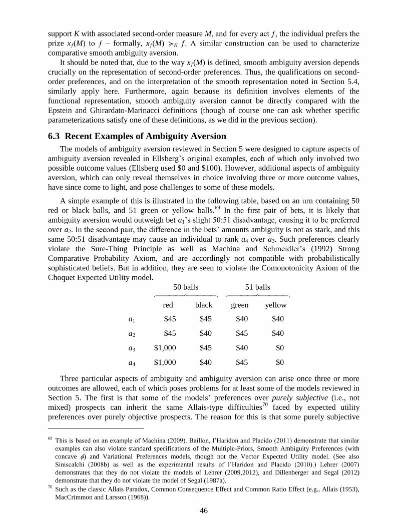
46
support K with associated second-order measure M, and for every act ƒ, the individual prefers the
prize xƒ(M) to ƒ – formally, xƒ(M) K ƒ. A similar construction can be used to characterize
comparative smooth ambiguity aversion.
It should be noted that, due to the way xƒ(M) is defined, smooth ambiguity aversion depends
crucially on the representation of second-order preferences. Thus, the qualifications on second-
order preferences, and on the interpretation of the smooth representation noted in Section 5.4,
similarly apply here. Furthermore, again because its definition involves elements of the
functional representation, smooth ambiguity aversion cannot be directly compared with the
Epstein and Ghirardato-Marinacci definitions (though of course one can ask whether specific
parameterizations satisfy one of these definitions, as we did in the previous section).
6.3 Recent Examples of Ambiguity Aversion
The models of ambiguity aversion reviewed in Section 5 were designed to capture aspects of
ambiguity aversion revealed in Ellsberg’s original examples, each of which only involved two
possible outcome values (Ellsberg used $0 and $100). However, additional aspects of ambiguity
aversion, which can only reveal themselves in choice involving three or more outcome values,
have since come to light, and pose challenges to some of these models.
A simple example of this is illustrated in the following table, based on an urn containing 50
red or black balls, and 51 green or yellow balls.69
In the first pair of bets, it is likely that
ambiguity aversion would outweigh bet a1’s slight 50:51 disadvantage, causing it to be preferred
over a2. In the second pair, the difference in the bets’ amounts ambiguity is not as stark, and this
same 50:51 disadvantage may cause an individual to rank a4 over a3. Such preferences clearly
violate the Sure-Thing Principle as well as Machina and Schmeidler’s (1992) Strong
Comparative Probability Axiom, and are accordingly not compatible with probabilistically
sophisticated beliefs. But in addition, they are seen to violate the Comonotonicity Axiom of the
Choquet Expected Utility model.
50 balls
51 balls
red black green yellow
a1 $45 $45 $40 $40
a2 $45 $40 $45 $40
a3 $1,000 $45 $40 $0
a4 $1,000 $40 $45 $0
Three particular aspects of ambiguity and ambiguity aversion can arise once three or more
outcomes are allowed, each of which poses problems for at least some of the models reviewed in
Section 5. The first is that some of the models’ preferences over purely subjective (i.e., not
mixed) prospects can inherit the same Allais-type difficulties70
faced by expected utility
preferences over purely objective prospects. The reason for this is that some purely subjective
69 This is based on an example of Machina (2009). Baillon, l’Haridon and Placido (2011) demonstrate that similar
examples can also violate standard specifications of the Multiple-Priors, Smooth Ambiguity Preferences (with
concave ) and Variational Preferences models, though not the Vector Expected Utility model. (See also
Siniscalchi (2008b) as well as the experimental results of l’Haridon and Placido (2010).) Lehrer (2007)
demonstrates that they do not violate the models of Lehrer (2009,2012), and Dillenberger and Segal (2012)
demonstrate that they do not violate the model of Segal (1987a). 70
Such as the classic Allais Paradox, Common Consequence Effect and Common Ratio Effect (e.g., Allais (1953),
MacCrimmon and Larsson (1968)).
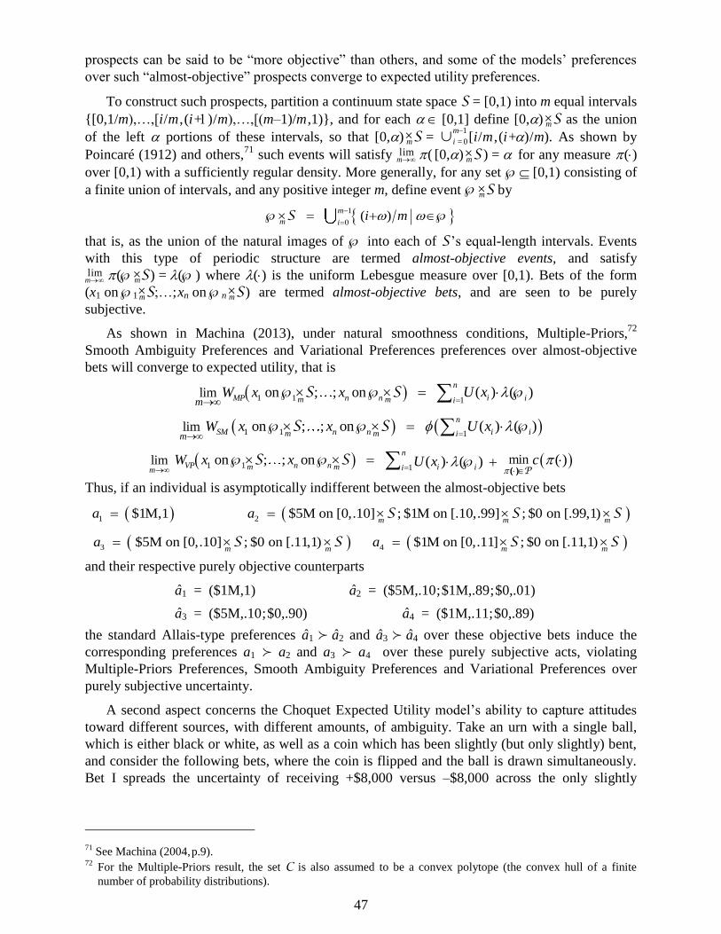
47
prospects can be said to be “more objective” than others, and some of the models’ preferences
over such “almost-objective” prospects converge to expected utility preferences.
To construct such prospects, partition a continuum state space S = [0,1) into m equal intervals
{[0,1/m),…,[i/m ,(i+)/m),…,[(m–1)/m ,1)}, and for each [0,1] define [0,)×mS as the union
of the left portions of these intervals, so that [0,)×mS =
m
i =
–1
0[i/m ,(i+)/m). As shown by
Poincaré (1912) and others,71
such events will satisfy mlim ( [0,)×
mS ) = for any measure ()
over [0,1) with a sufficiently regular density. More generally, for any set [0,1) consisting of
a finite union of intervals, and any positive integer m, define event ×mS by
1
0( )
m
m ii m
S
that is, as the union of the natural images of into each of S’s equal-length intervals. Events
with this type of periodic structure are termed almost-objective events, and satisfy
mlim (×mS) = () where () is the uniform Lebesgue measure over [0,1). Bets of the form
(x1 on 1×mS;…;xn on n×mS) are termed almost-objective bets, and are seen to be purely
subjective.
As shown in Machina (2013), under natural smoothness conditions, Multiple-Priors,72
Smooth Ambiguity Preferences and Variational Preferences preferences over almost-objective
bets will converge to expected utility, that is
1 1 1lim ( )on ; ; on ( )
n
iMP n n im m imU xW x x
S S
1 1 1lim on ; ; on ( ) ( )
n
SM n n i im m imW x x U x
S S
1 1 1minlim on ; ; on ( )( ) ( )
n
VP n nm m i iimW x x cU x
( ) PS S
Thus, if an individual is asymptotically indifferent between the almost-objective bets
1 2
3 4
$1M,1 $5M on [0,.10] ; $1M on [.10,.99] ; $0 on [.99,1)
$5M on [0,.10] ; $0 on [.11,1) $1M on [0,.11] ; $0 on [.11,1)
m m m
m m m m
a a
a a
S S S
S S S S
and their respective purely objective counterparts
a1 = ($1M,1) a2 = ($5M,.10;$1M,.89;$0,.01)
a3 = ($5M,.10;$0,.90) a4 = ($1M,.11;$0,.89)
the standard Allais-type preferences a1 a2 and a3 a4 over these objective bets induce the
corresponding preferences a1 a2 and a3 a4 over these purely subjective acts, violating
Multiple-Priors Preferences, Smooth Ambiguity Preferences and Variational Preferences over
purely subjective uncertainty.
A second aspect concerns the Choquet Expected Utility model’s ability to capture attitudes
toward different sources, with different amounts, of ambiguity. Take an urn with a single ball,
which is either black or white, as well as a coin which has been slightly (but only slightly) bent,
and consider the following bets, where the coin is flipped and the ball is drawn simultaneously.
Bet I spreads the uncertainty of receiving +$8,000 versus –$8,000 across the only slightly
71 See Machina (2004,p.9).
72 For the Multiple-Priors result, the set C is also assumed to be a convex polytope (the convex hull of a finite
number of probability distributions).
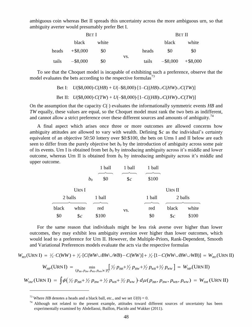
48
ambiguous coin whereas Bet II spreads this uncertainty across the more ambiguous urn, so that
ambiguity averter would presumably prefer Bet I.
BET I BET II
black white black white
heads +$8,000 $0 vs.
heads $0 $0
tails –$8,000 $0 tails –$8,000 +$8,000
To see that the Choquet model is incapable of exhibiting such a preference, observe that the
model evaluates the bets according to the respective formulas73
Bet I: U($8,000)C(HB) + U(–$8,000)[1–C((HB)C(HW)C(TW)]
Bet II: U($8,000)C(TW) + U(–$8,000)[1–C((HB)C(HW)C(TW)]
On the assumption that the capacity C() evaluates the informationally symmetric events HB and
TW equally, these values are equal, so the Choquet model must rank the two bets as indifferent,
and cannot allow a strict preference over these different sources and amounts of ambiguity.74
A final aspect which arises once three or more outcomes are allowed concerns how
ambiguity attitudes are allowed to vary with wealth. Defining $c as the individual’s certainty
equivalent of an objective 50:50 lottery over $0:$100, the bets on Urns I and II below are each
seen to differ from the purely objective bet b0 by the introduction of ambiguity across some pair
of its events. Urn I is obtained from bet b0 by introducing ambiguity across it’s middle and lower
outcome, whereas Urn II is obtained from b0 by introducing ambiguity across it’s middle and
upper outcome.
1 ball 1 ball 1 ball
b0 $0 $c $100
URN I URN II
2 balls 1 ball 1 ball 2 balls
black white red vs. red black white
$0 $c $100
$0 $c $100
For the same reason that individuals might be less risk averse over higher than lower
outcomes, they may exhibit less ambiguity aversion over higher than lower outcomes, which
would lead to a preference for Urn II. However, the Multiple-Priors, Rank-Dependent, Smooth
and Variational Preferences models evaluate the acts via the respective formulas
2 1 13 2 3RN RN(U I) ( ) [ ( ) ( )] [1 ( )] (U II)RD RDW C WW C WW BW WB C WW C WW BW WB W
0
1 1 1 23 2 2 3
, )( , ,minRN RN(U I) (U II)
BB BW WB WW
MP BB BW WB WW MPp p pp
W p p p p W
P
1 1 1 23 2 2 3RN RN(U I) ( , , , ) (U II)SM BB BW WB WW BB BW WB WW SMW p p p p d p p p p W
73 Where HB denotes a heads and a black ball, etc., and we set U(0) = 0.
74 Although not related to the present example, attitudes toward different sources of uncertainty has been
experimentally examined by Abdellaoui, Baillon, Placido and Wakker (2011).
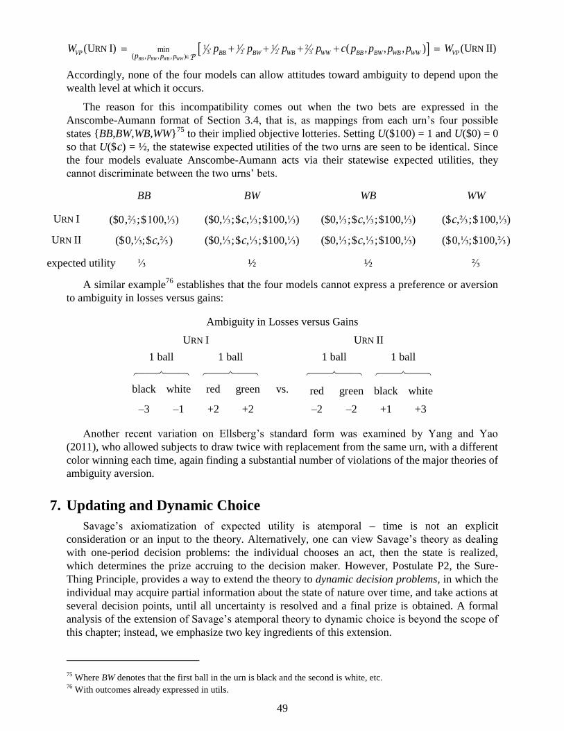
49
1 1 1 23 2 2 3
, )( , ,minRN RN(U I) ( , , , ) (U II)
BB BW WB WW
VP BB BW WB WW BB BW WB WW VPp p pp
W p p p p c p p p p W
P
Accordingly, none of the four models can allow attitudes toward ambiguity to depend upon the
wealth level at which it occurs.
The reason for this incompatibility comes out when the two bets are expressed in the
Anscombe-Aumann format of Section 3.4, that is, as mappings from each urn’s four possible
states {BB,BW,WB,WW}75
to their implied objective lotteries. Setting U($100) = 1 and U($0) = 0
so that U($c) = ½, the statewise expected utilities of the two urns are seen to be identical. Since
the four models evaluate Anscombe-Aumann acts via their statewise expected utilities, they
cannot discriminate between the two urns’ bets.
BB BW WB WW
URN I ($0,⅔;$100,⅓) ($0,⅓;$c,⅓;$100,⅓) ($0,⅓;$c,⅓;$100,⅓) ($c,⅔;$100,⅓)
URN II ($0,⅓;$c,⅔) ($0,⅓;$c,⅓;$100,⅓) ($0,⅓;$c,⅓;$100,⅓) ($0,⅓;$100,⅔)
expected utility ⅓ ½ ½ ⅔
A similar example76
establishes that the four models cannot express a preference or aversion
to ambiguity in losses versus gains:
Ambiguity in Losses versus Gains
URN I URN II
1 ball 1 ball
1 ball 1 ball
black white red green vs. red green black white
–3 –1 +2 +2
–2 –2 +1 +3
Another recent variation on Ellsberg’s standard form was examined by Yang and Yao
(2011), who allowed subjects to draw twice with replacement from the same urn, with a different
color winning each time, again finding a substantial number of violations of the major theories of
ambiguity aversion.
7. Updating and Dynamic Choice
Savage’s axiomatization of expected utility is atemporal – time is not an explicit
consideration or an input to the theory. Alternatively, one can view Savage’s theory as dealing
with one-period decision problems: the individual chooses an act, then the state is realized,
which determines the prize accruing to the decision maker. However, Postulate P2, the Sure-
Thing Principle, provides a way to extend the theory to dynamic decision problems, in which the
individual may acquire partial information about the state of nature over time, and take actions at
several decision points, until all uncertainty is resolved and a final prize is obtained. A formal
analysis of the extension of Savage’s atemporal theory to dynamic choice is beyond the scope of
this chapter; instead, we emphasize two key ingredients of this extension.
75 Where BW denotes that the first ball in the urn is black and the second is white, etc.
76 With outcomes already expressed in utils.
50
The first is updating. The notion of updating a prior probability measure so as to reflect
information the individual has acquired is familiar. If one assumes that the individual is an
expected utility maximizer, and that his or her risk attitudes and tastes do not change, the
probabilistic conditioning operator determines a conditional preference. Savage (1954,p.22)
suggested the converse approach: one can start with a definition of conditional preference, and
show that it characterizes probabilistic updating. Specifically, Savage stipulates that act ƒ is
weakly preferred to act g given event E, written ƒ E g, if and only if, for some act h,
(ƒ,E;h ,~E) (g ,E;h ,~E) (20)
It is easy to see that, if the ex-ante preference is an EU preference, with subjective prior ,
then the updated preference E is also consistent with EU. Then, if the event E is nonnull,77
one
has µ(E) > 0, and the probability measure associated with the updated preference E is the usual
update (∙ |E) of . We emphasize that Postulate P2 is essential to ensure that this definition is
well-posed: if P2 is violated, then different choices of acts h may lead to contradictory rankings
of ƒ and g conditional on E.
The second key ingredient in the extension of Savage’s theory to dynamic choice is dynamic
consistency. One possible formulation of this property is as follows: if act ƒ is weakly preferred
to act g conditional on E, and also conditional on ~E, then ƒ is unconditionally preferred to g;
also, if one of the conditional preferences is strict, so is the unconditional preference. Formally:
ƒ E g, ƒ ~E g ƒ g ƒ E g, ƒ ~E g ƒ g (21)
(The second part of the definition requires that the event E be nonnull.) Dynamic consistency is
essential to ensure that, if a multi-period choice problem is solved by backward induction or
recursion, one obtains a solution that is also optimal ex-ante. It turns out that Savage’s Postulate
P2 also ensures that conditional preferences as defined above satisfy dynamic consistency.
(Indeed, the connection between P2 and dynamic consistency is tight: see Epstein and Le Breton
(1993), Ghirardato (2002) and Siniscalchi (2011,Sect.4.2).)
Since ambiguity-sensitive preferences violate Postulate P2, it should come as no surprise that
updating and consistent dynamic choice pose challenges. As we shall see, there is no unique way
to define conditional preferences or – in any given parametric model – conditional “beliefs.”
Furthermore, no matter how we define conditional preferences, we can construct examples in
which dynamic consistency is violated. Different approaches have been proposed to deal with
these issues. We now briefly discuss some of the relevant contributions.
Lack of space prevents us from discussing two other broadly related issues which have seen
recent work. The first is learning under ambiguity: see Epstein and Schneider (2007). The second
is the notion of exchangeability, or symmetry: Epstein and Seo (2010a,2010b,2012) extend the
classic results of de Finetti (1937) and Hewitt and Savage (1955) to ambiguity-sensitive
preferences. See also Al Najjar and De Castro (2013).
7.1 Updating Ambiguous Beliefs
Early contributions focus on updating rules for capacities in the Choquet Expected Utility
model. Two rules have received particular attention: the Dempster-Shafer Rule and the Full
Bayesian Rule. Both essentially originate in the work of Dempster (1967), who considers the
following scenario: An individual has a probabilistic belief on a set ; furthermore, there is a
correspondence (a multivalued map) : S , where S is the state space of interest, which for
77 See footnote 25.
51
simplicity we assume to be finite. Intuitively, the map describes the individual’s partial
information about the relationship between elements of , whose likelihood the individual can
assess with confidence, and the events in S. The individual’s beliefs on S are represented by the
capacity defined by
: ( )( )
: ( )
Av A
Intuitively, this embodies a conservative stance: the individual assigns to each A only the
probability of those elements of that he or she knows for sure to correspond to elements in A.
The capacity thus defined is convex, and indeed satisfies a stronger property that characterizes
so-called “belief functions” (e.g., Shafer (1976) and Jaffray (1992)). The reason why Γ is
allowed to take on an empty value will be clear momentarily.
Dempster describes the following updating rule. Suppose the individual learns that event E
𝒮 has occurred. The initial information, as encoded by Γ, was that element ω of Ω mapped to
states s in (): but since he or she now knows that the state s must also lie in E, he or she
associates with () ∩ E. We can then define E()=() ∩ E and construct the capacity
DS(∙ |E) derived from E as above (we explain the superscript below). Dempster shows that
[ ] [~ ] (~ )( | )
1 (~ )DS
v A E E v Ev A E
v E
While this expression may seem a bit mysterious, the above construction clarifies its origin.
The subsequent literature has mostly taken the above formula (or alternative, equivalent
formulae) as the definition of a particular updating rule; since it also plays a prominent role in the
work of Shafer (1976), it is commonly referred to as the Dempster-Shafer updating rule (hence
the subscript in DS(∙ |E)).
An alternative updating rule for capacities is related to sets of priors. It is known that, if a
capacity v is a “belief function,” then it satisfies the following duality relation: letting 𝒞v be the
set of probability distributions µ such that µ(A) ≥ v(A) for all events A, it is the case that, for
every event A, (A) = inf {µ(A) : µ 𝒞v} (this is not true for arbitrary convex capacities). Thus,
a possible updating rule is as follows: first, assuming v(E) > 0, update all probability
distributions in 𝒞v according to the usual probabilistic conditioning formula; then, consider the
lower envelope of the resulting set. That is, we define the so-called Full Bayesian updating rule
for the belief function by FB(A|E) = inf {µ(A|E):µ 𝒞v}. Jaffray (1992) shows that vFB(∙|E) is
indeed a belief function, and furthermore that
( )
( | )( ) 1 ~
FB
v Av A E
v A v A E
An alternative approach leading to the above definition of Full Bayesian updating can be found
in Fagin and Halpern (1991).
Gilboa and Schmeidler (1993) are the first to provide an axiomatic treatment of updating
rules in a decision setting; in particular, they adopt the horse-roulette act environment discussed
in Section 5, and assume that there exist a best and a worst prize. They consider uncertainty-
averse Choquet Expected Utility preferences (which are thus also Maxmin Expected Utility
preferences) and consider the class of h-Bayesian update rules, where h is an arbitrary act. Given
an unconditional preference ≽, the h-Bayesian update given E, denoted ≽E,h, is defined by
ƒ E,h g (ƒ,E;h ,E) (g ,E;h ,E)
52
Under Savage’s Postulate P2, all h-Bayesian update rules coincide with Savage’s update rule;
however, for more general preferences, different choices of h induce different conditional
preferences. In particular, Gilboa and Schmeidler show that, if one takes h to be the constant act
that yields the best possible prize, the resulting conditional preference is CEU, with capacity
given by the Dempster-Shafer update of the prior capacity (the utility function is unchanged
relative to the prior preference). They interpret this as a form of “pessimistic updating”: when
receiving the information that E has occurred, the individual ranks acts as if, in the
counterfactual event, he or she would have received the best possible prize.
Eichberger, Grant and Kelsey (2007) and Horie (2007) characterize Full Bayesian updating
for arbitrary capacities. Their main axiom is adopted from Pires (2002), a paper we discuss
below; thus, we defer the discussion of their contribution.
Two main updating rules have been proposed for maxmin expected utility (MEU)
preferences. The first stipulates that, given a set 𝒞 of priors on the state space 𝒮, all priors µ 𝒞
with µ(∙|E) > 0 be updated upon learning that E has occurred; this is called the Full or
Generalized Bayesian updating rule for the set 𝒞. It is related to Full Bayesian updating for
belief functions, in the sense that (i) a CEU preference for which the capacity is a belief function,
and hence convex, is also a MEU preference, and (ii) by the result stated above, the CEU
preference characterized by the full Bayesian update of the capacity is the same as the MEU
preference characterized by the full Bayesian update of the set 𝒞. However, it is important to
emphasize that full Bayesian updating of sets of priors is well-defined for arbitrary sets 𝒞, not
just those that consist of probability distributions that dominate a given belief function.
Full Bayesian updating of priors has been axiomatized by Pires (2002) in the horse-roulette
act setup; related results can be found in Walley (1991,pp.632-638) and Jaffray (1994). The key
axiom establishes a connection between the conditional certainty equivalent x of an act ƒ and
unconditional ranking of x vis-à-vis a suitable composite act: formally, for every (nonnull) event
E, act ƒ and prize x, it requires that ƒ~E x if and only if (ƒ,E ;x ,~E) ~ x. One implication of this
axiom is that conditional preferences can be elicited from prior preferences: this is done by
determining, for each act ƒ, the prize x that solves the preference equation (ƒ,E; x,~E) ~ x.78
Eichberger, Grant and Kelsey (2007) use the same axiom to characterize Full Bayesian
Updating for capacities; however, Horie (2007) points out that, while Pires’s axiom is sufficient
to deliver full Bayesian updating, it is too strong. Horie shows that the appropriate necessary and
sufficient condition is a version of Pires’s axiom that is restricted to binary acts ƒ.
An alternative updating rule was proposed and characterized by Gilboa and Schmeidler
(1993). Recall that they characterize Dempster-Shafer updating for uncertainty averse CEU
preferences, which are thus also MEU preferences. Hence, their result necessarily also pins down
a procedure to update sets of priors. The procedure works as follows: out of the set 𝒞 of priors
characterizing the ex-ante preference, select the measures assigning the maximum probability to
the event E that has occurred, and only update those. Gilboa and Schmeidler call this the
maximum-likelihood update rule. Note that their characterization result only covers preferences
that are both MEU and CEU; a characterization of maximum-likelihood updating for general
MEU preferences is not known.
Finally, Siniscalchi (2009a) defines and axiomatizes an updating rule for VEU preferences,
which entails (i) updating the baseline prior in the usual way, and (ii) replacing the covariances
in equation (10) with suitably rescaled conditional covariances.
78 Siniscalchi (2011) shows that Pires’s axiom is equivalent to a weakening of the standard dynamic consistency
property discussed above.
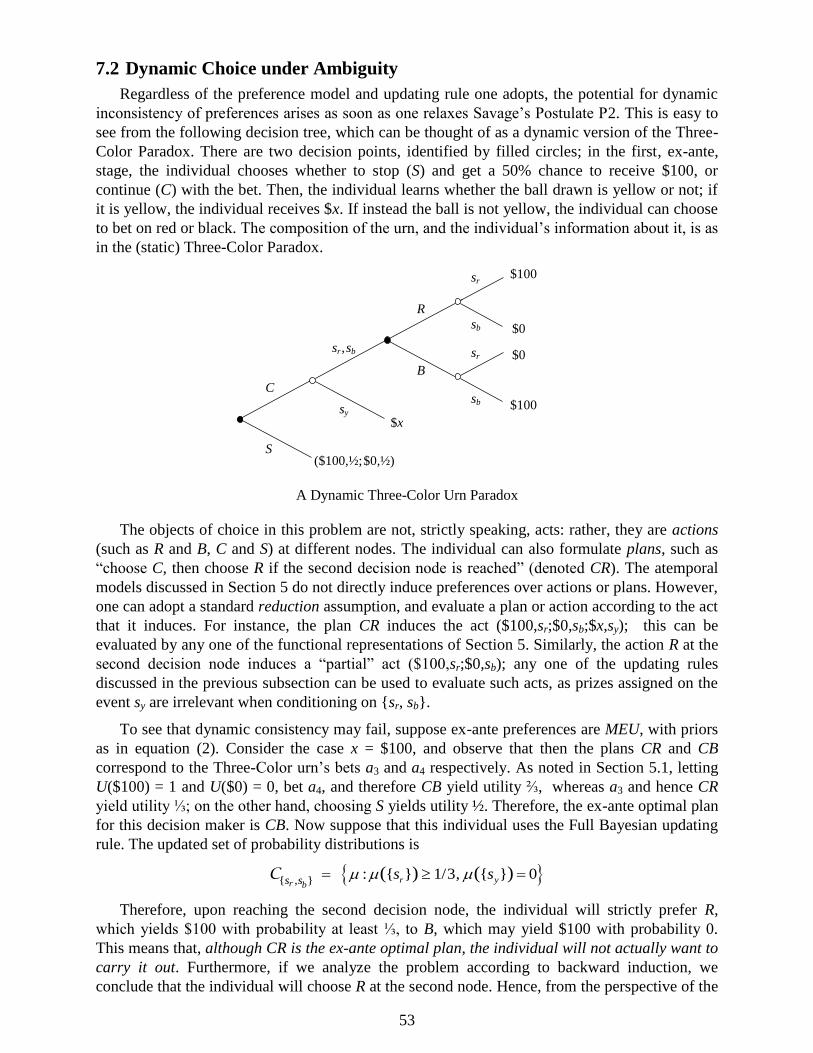
53
7.2 Dynamic Choice under Ambiguity
Regardless of the preference model and updating rule one adopts, the potential for dynamic
inconsistency of preferences arises as soon as one relaxes Savage’s Postulate P2. This is easy to
see from the following decision tree, which can be thought of as a dynamic version of the Three-
Color Paradox. There are two decision points, identified by filled circles; in the first, ex-ante,
stage, the individual chooses whether to stop (S) and get a 50% chance to receive $100, or
continue (C) with the bet. Then, the individual learns whether the ball drawn is yellow or not; if
it is yellow, the individual receives $x. If instead the ball is not yellow, the individual can choose
to bet on red or black. The composition of the urn, and the individual’s information about it, is as
in the (static) Three-Color Paradox.
A Dynamic Three-Color Urn Paradox
The objects of choice in this problem are not, strictly speaking, acts: rather, they are actions
(such as R and B, C and S) at different nodes. The individual can also formulate plans, such as
“choose C, then choose R if the second decision node is reached” (denoted CR). The atemporal
models discussed in Section 5 do not directly induce preferences over actions or plans. However,
one can adopt a standard reduction assumption, and evaluate a plan or action according to the act
that it induces. For instance, the plan CR induces the act ($100,sr;$0,sb;$x,sy); this can be
evaluated by any one of the functional representations of Section 5. Similarly, the action R at the
second decision node induces a “partial” act ($100,sr;$0,sb); any one of the updating rules
discussed in the previous subsection can be used to evaluate such acts, as prizes assigned on the
event sy are irrelevant when conditioning on {sr, sb}.
To see that dynamic consistency may fail, suppose ex-ante preferences are MEU, with priors
as in equation (2). Consider the case x = $100, and observe that then the plans CR and CB
correspond to the Three-Color urn’s bets a3 and a4 respectively. As noted in Section 5.1, letting
U($100) = 1 and U($0) = 0, bet a4, and therefore CB yield utility ⅔, whereas a3 and hence CR
yield utility ⅓; on the other hand, choosing S yields utility ½. Therefore, the ex-ante optimal plan
for this decision maker is CB. Now suppose that this individual uses the Full Bayesian updating
rule. The updated set of probability distributions is
{ , }: { } 1/3, { } 0( ) ( )r yr bs s
s s C
Therefore, upon reaching the second decision node, the individual will strictly prefer R,
which yields $100 with probability at least ⅓, to B, which may yield $100 with probability 0.
This means that, although CR is the ex-ante optimal plan, the individual will not actually want to
carry it out. Furthermore, if we analyze the problem according to backward induction, we
conclude that the individual will choose R at the second node. Hence, from the perspective of the
$100
$0
$100
$0
R
B
$x
sb
sr
sr
sb
C
S
sr,sb
sy
($100,½;$0,½)
54
first node, choosing C is “just as good” as committing to plan CB, which – as noted above – has
an ex-ante utility of only ⅓. Therefore, the individual will prefer to choose S at the initial node,
according to backward induction. Thus, backward induction yields a different solution than ex-
ante optimization. Both these issues can be traced back to a violation of dynamic consistency: the
acts a4 and a3 (equivalently, the plans CR and CB) are indifferent conditional on {sy} because
they both yield $x = $100, the individual strictly prefers a3 to a4 conditional on {sr, sb}, but
strictly prefers a4 to a3 unconditionally.
Similar examples can be constructed for different preference representations and updating
rules; the issues highlighted are not unique to MEU or full Bayesian updating.
There are three ways to address this failure of dynamic consistency.79
The first was
introduced by Epstein and Schneider (2003) in the context of MEU preferences, and extended to
Variational Preferences by Maccheroni, Marinacci and Rustichini (2006b), to Smooth Ambiguity
Preferences by Klibanoff, Marinacci and Mukerji (2009), and to Vector Expected Utility
preferences by Siniscalchi (2010). This approach has also been broadly adopted in applications,
especially in financial economics. The basic observation is that the noted tight connection
between Savage’s Postulate P2 and dynamic consistency does not prevent the coexistence of
some departures from P2 and some form of dynamic consistency. More precisely, if for a given
state space one wishes to ensure dynamic consistency in every possible decision tree, then
Postulate P2 must hold for all events, and therefore there is no scope for Ellsberg behavior.
However, one can fix one particular decision tree, and require dynamic consistency only for that
particular tree. This implies that P2 will hold only for some events, but there will still be scope
for Ellsberg-type behavior.
For a simple example, suppose that a fair coin is tossed; if it comes up heads, the individual
is confronted with the Three-Color Ellsberg urn and must choose to bet on red vs. black; if it
comes up tails, the individual faces the same urn but must choose whether to bet on red or yellow
vs. black or yellow. Letting the space be S = {H ,T}×{r ,b ,y} to simplify notation, a plausible
set of priors for this problem is
1
6: { } { } , { } { } , { } { }( ) ( ) ( ) ( ) ( ) ( )r r y yb bH T H T H T C
For this set of priors, the modal Ellsberg preferences obtain, both ex-ante and after each
realization of the coin toss. Dynamic consistency also holds in this tree. Note that this set of
priors is obtained by taking the product of the uniform probability on {H ,T} with the priors in
the set C of equation (2). Epstein and Schneider show that dynamic consistency of MEU
preferences in a particular tree characterizes a generalization of this property of the representing
set of priors, called rectangularity. Furthermore, they show that dynamic MEU preferences with
a rectangular set of priors admit a recursive representation; this accounts for the popularity of
this approach in applications.
Rectangularity does rule out, for example, the set of priors in equation (2) from Section 5.1,
which we used to analyze the dynamic version of the Three-Color Paradox in the above figure.
Intuitively, conditioning on the event {sr,sb} “breaks” the complementarity between the states sb
and sy (cf. Section 5.6 and 6.1) and this leads to a violation of dynamic consistency. Loosely
speaking, rectangularity rules out precisely these complementarities across different conditioning
events. Of course, in some contexts, such complementarities may be the main object of interest –
79 A fourth way is to drop the reduction assumption. In the example, one could argue that the individual may prefer
plan CR to plan CB in the tree of the figure, even though he or she prefers act a4 to act a3 in the static Three-Color
Paradox. This is explored in Li (2011).
55
as is the case in the stylized problem of the figure. In such cases, alternatives to the Epstein-
Schneider approach can be pursued.
One such alternative was advocated by Hanany and Klibanoff (2007,2009), who adapt
arguments first proposed by Machina (1989) in the context of risky choice. The basic intuition is
that the preceding arguments implicitly made the assumption that, when the individual is
evaluating choices at a node in a decision tree, bygones are bygones: the only relevant
considerations are the residual uncertainty, and the prizes delivered at terminal nodes that can
still be reached. Machina, as well as Hanany and Klibanoff, argue that this need not be the case.
For example, in the choice problem of the figure, when the individual faces a choice between R
and B, he or she may take into account that this choice occurs “in the context” of a given
decision tree. In particular, he or she may take into account the prize $x that would have been
delivered if a yellow ball had been drawn. Formally, this allows the individual to express a
conditional preference for R over B if x = $0, and for B over R if x = $100. Hence, in particular,
with x = $100 there no longer is any dynamic inconsistency: ex-ante, the individual prefers CB to
CR, and upon reaching the second decision node, prefers B to R.
Formally, Hanany and Klibanoff (2007) focus on MEU preferences, and impose a (weak)
form of dynamic consistency. They consider a class of two-period decision problems and a class
of updating rules, i.e., mappings that associate a second-period conditional preference to every
prior preference, decision problem and ex-ante optimal act. Within this class, they characterize
the ones that are dynamically consistent in the sense that the ex-ante optimal act remains
conditionally optimal. Their 2009 paper extends the results to arbitrary Uncertainty-Averse
Preferences.
One consequence of this approach is that the resulting conditional preferences may display
either uncertainty aversion or uncertainty neutrality, depending on the prizes assigned at
counterfactual terminal nodes; an example is provided in Siniscalchi (2009b). This seems at odds
with the usual interpretation of ambiguity, which concerns information rather than prizes.
The final approach we discuss can be traced back to Strotz (1956), and was advocated in the
context of ambiguity by Siniscalchi (2011). The basic idea is to assume that individuals are
sophisticated: that is, even though they may be dynamically inconsistent, they correctly
anticipates their future behavior, and respond accordingly. Strotz argues that a sophisticated
individual should engage in a strategy of consistent planning: at each decision point, they should
choose the plan that is best according to their current preferences, among all those plans that, in
view of their future preferences, they will actually be able to carry out. Consistent planning is
thus a “refinement” of backward induction, in the sense that, whenever two or more plans are
optimal from the perspective of future preferences, the one that is optimal for the current
preferences is selected.
In the tree of the figure with x = $100, consistent planning implies that, at the initial node, the
individual will anticipate their preference for R over B upon learning that a yellow ball was not
drawn; hence, they will realize that choosing C is tantamount to committing to the plan CR, and
will therefore choose S instead. In other words, consistent planning coincides with backward
induction in this example.
Siniscalchi provides an axiomatization of consistent planning. The key insight is that, to
formulate the sophistication principle (and other assumptions implicit in consistent planning),
preferences need to be defined over decision trees, rather than acts, or even plans. This is
analogous to the use of preferences over menus in the literature on preference for flexibility, or
56
temptation and self-control. One advantage of this approach is that it yields insight into the issue
of the value of information under ambiguity. The reader is referred to the original paper for detail
8. Conclusion
In recent decades the theoretical and experimental literature on the economics of ambiguity
and ambiguity aversion spawned by Ellsberg (1961,1962) has exploded to the point where it is
much too extensive to be covered in a single chapter of this form. For additional discussion, the
reader is referred to the surveys of Sugden (1986), Camerer and Weber (1992), Kelsey and
Quiggin (1992), Kischka and Puppe (1992), Camerer (1995), Mukerji (2000), Starmer (2000),
Siniscalchi (2008a), Gilboa, Postlewaite and Schmeidler (2008) Al-Najjar and Weinstein (2009),
Hey, Lotito and Maffioletti (2010), Etner, Jeleva and Tallon (2012) and Gilboa and Marinacci
(2012), the journal symposium issues of Bonanno, Van Hees, List and Tungodden (2009) and
Ellsberg, Machina, Ritzberger and Yannelis (2011), and the extensive annotated bibliography of
Wakker (2013).
57
REFERENCES
Abdellaoui, M., Baillon, A., Placido, L., Wakker, P. (2011). “The Rich Domain of Uncertainty:
Source Functions and Their Experimental Implementation”. American Economic Review
101, 695-723
Ahn, D. S. (2008). “Ambiguity Without a State Space”. Review of Economic Studies 75, 3-28.
Al Najjar, N., De Castro, L. (2013). “Parametric Representation of Preferences”. manuscript.,
Kellogg Graduate School of Management, Northwestern University.
Al-Najjar, N., Weinstein J. (2009). “The Ambiguity Aversion Literature: A Critical
Assessment”. Economics and Philosophy 25, 249-284.
Allais, M. (1953). “Le Comportement de l’Homme Rationnel Devant Le Risque, Critique des
Postulats et Axiomes de l’Ecole Américaine”. Econometrica 21, 503-546.
Anscombe F., Aumann, R. (1963). “A Definition of Subjective Probability”. Annals of
Mathematical Statistics 34, 199-205.
Arrow, K. (1951). “Alternative Approaches to the Theory of Choice in Risk-Taking Situations”.
Econometrica 19, 404-437.
Arrow, K. (1963). “Comment”. Review of Economics and Statistics 45 (Supplement), 24-27.
Baillon, A., Cabantous, L., Wakker, P. (2012). “Aggregating Imprecise or Conflicting Beliefs:
An Experimental Investigation Using Modern Ambiguity Theories”. Journal of Risk and
Uncertainty 44, 115-147.
Baillon, A., l’Haridon, O., Placido, L. (2011). “Ambiguity Models and the Machina Paradoxes”.
American Economic Review 101, 1547-1560.
Baillon, A., Bleichrodt, H. (2011). “Testing Ambiguity Models Through the Measurement of
Probabilities for Gains and Losses”. manuscript. Erasmus University Rotterdam.
Bayes, T. (1763). “An Essay toward Solving a Problem in the Doctrine of Chances”.
Philosophical Transactions of the Royal Society of London 53, 370-418.
Becker, G., DeGroot, M., Marschak, J. (1964). “Measuring Utility by a Single-Response
Sequential Method”. Behavioral Science 9, 226-232.
Becker, S., Brownson, F. (1964). “What Price Ambiguity? Or the Role of Ambiguity in
Decision-Making”. Journal of Political Economy 72, 62-73.
Bernoulli, D. (1738). “Specimen Theoriae Novae De Mensura Sortis,” Commentarii Academiae
Scientiarum Imperialis Petropolitanae [Papers of the Imperial Academy of Sciences in
Petersburg] V, 175-192. English Translation: “Exposition of a New Theory on the
Measurement of Risk,” Econometrica 22 (1954), 23-36.
Bewley, T. (2002). “Knightian Decision Theory. Part 1”. Decisions in Economics and Finance
25, 79-110.
Bewley, T. (2011). “Market Innovation and Entrepreneurship: A Knightian View”. in Debreu,
G., Neuefeind, W., Trockel, W. (eds.) Economics Essays: A Festschrift for Werner
Hildenbrand, Springer.
Bonanno, G., Van Hees, M., List, C., Tungodden, B. (2009). “Special Issue on Ambiguity
Aversion”. Economics and Philosophy 25, 247-369.
58
Brewer, K. (1963). “Decisions under Uncertainty: Comment,” Quarterly Journal of Economics
77, 159-161.
Brewer, K., Fellner, W. (1965). “The Slanting of Subjective Probabilities – Agreement on Some
Essentials,” Quarterly Journal of Economics 79, 657-663.
Camerer, C. (1995). “Individual Decision Making”. in Kagel, J., Roth, A. (eds.) Handbook of
Experimental Economics. Princeton: University Press.
Camerer, C., Kunreuther, H. (1989a). “Decision Processes for Low Probability Events: Policy
Implications”. Journal of Policy Analysis and Management 8, 565-592.
Camerer, C., Kunreuther, H. (1989b). “Experimental Markets for Insurance”. Journal of Risk and
Uncertainty 2, 265-300.
Camerer, C., Weber, M. (1992). “Recent Developments in Modeling Preferences: Uncertainty
and Ambiguity”. Journal of Risk and Uncertainty 5, 325-370.
Carter, C. (1950). “Expectation in Economics” (Review of Shackle (1949a)). Economic Journal
60, 92-105
Casadesus-Masanell, R., Klibanoff, P. Ozdenoren, E. (2000a). “Maxmin Expected Utility Over
Savage Acts with a Set of Priors”. Journal of Economic Theory 92, 33-65.
Casadesus-Masanell, R., Klibanoff, P. Ozdenoren, E. (2000b). “Maxmin Expected Utility
Through Statewise Combinations”. Economics Letters 66, 49-54.
Cerreia-Vioglio, S., Ghirardato, P., Maccheroni, F., Marinacci, M., Siniscalchi, M. (2011).
“Rational Preferences under Ambiguity”. Economic Theory 48, 341-375.
Cerreia-Vioglio, S., Maccheroni, F., Marinacci, M., Montrucchio, L. (2011). “Uncertainty
Averse Preferences”. Journal of Economic Theory 146, 1275-1330.
Chambers, R., Grant, S., B. Polak, B., Quiggin, J. (2013). “A Two-Parameter Model of
Dispersion Aversion”. manuscript, University of Queensland.
Chateauneuf, A., Faro. J. (2009). “Ambiguity Through Confidence Functions”. Journal of
Mathematical Economics 45, 535-558.
Chernoff, H. (1954). “Rational Selection of Decision Functions”. Econometrica 22, 422-443.
Chew, S., Li, K., Chark, R., Zhong, S. (2008). “Source Preference and Ambiguity Aversion:
Models and Evidence from Behavioral and Neuroimaging Experiments” In Neuroeconomics.
Advances in Health Economics and Health Services Research 20, 179-201.
Chew, S.H., Sagi, J. (2006). “Event Exchangeability: Probabilistic Sophistication Without
Continuity or Monotonicity”. Econometrica 74, 771-786.
Chew, S.H.. Sagi, J. (2008). “Small Worlds: Modeling Attitudes Toward Sources of
Uncertainty”. Journal of Economic Theory 139, 1-24.
Chipman, (1958). “Stochastic Choice and Subjective Probability (Abstract)”. Econometrica 26,
613.
Chipman, J. (1960). “Stochastic Choice and Subjective Probability”. in D. Willner (ed.)
Decisions, Values and Groups, New York, Pergamon Press, 1960.
Chow, C., Sarin, R. (2001). “Comparative Ignorance and the Ellsberg Paradox”. Journal of Risk
and Uncertainty 22, 129-139.
Clarke, F. H. (1983). Optimization and Nonsmooth Analysis. Wiley-Interscience, New York.
59
Cohen, M., Jaffray, J.-Y., Said, T. (1985). “Individual Behavior under Risk and under
Uncertainty: An Experimental Study”. Theory and Decision 18, 203-228.
Cohen, M., Jaffray, J.-Y., Said, T. (1987). “Individual Behavior under Risk and under
Uncertainty for Gains and Losses”. Organizational Behavior and Human Decision Processes
39, 1-22.
Curley, S., Eraker, S., Yates, F. (1984). “An Investigation of Patient's Reactions To Therapeutic
Uncertainty”. Medical Decision Making 4, 501-511.
Curley, S., Yates, F. (1985). “The Center and Range of the Probability Interval As Factors
Affecting Ambiguity Preferences,” Organizational Behavior and Human Decision Processes
36, 272-287.
Curley, S., Yates, F. (1989). “An Empirical Evaluation of Descriptive Models of Ambiguity
Reactions in Choice Situations,” Journal of Mathematical Psychology 33, 397-427.
Curley, S., Young, M., Yates, F. (1989). “Characterizing Physicians’ Perceptions of Ambiguity,"
Medical Decision Making 9, 116-124.
Davidson, D., Suppes, P. (1956). “A Finitistic Axiomatization of Utility and Subjective
Probability”. Econometrica 24, 264-275.
de Finetti, B. (1937). “La Prévision: Ses Lois Logiques, Ses Sources Subjectives”. Annales De
L'institut Henri Poincaré 7, 1-68.
DeGroot, M. (1970). Optimal Statistical Decisions. New York: McGraw-Hill Book Co.
Dempster, A. (1967). “Upper and Lower Probabilities Induced by a Multivalued Mapping”.
Annals of Mathematical Statistics 38, 325-339.
Dillenberger, D., Segal, U. (2012). “Recursive Ambiguity and Machina’s Examples”.
manuscript, University of Pennsylvania.
Du, N., Budescu, D. (2005). “The Effects of Imprecise Probabilities and Outcomes in Evaluating
Investment Options”. Management Science 51, 1791-1803.
Dumav, M., Stinchcombe, M. (2013). “The von Neumann-Morgenstern Approach To
Ambiguity”. manuscript, University of Texas at Austin.
Eichberger, J., Grant, S., Kelsey, D. (2007). “Updating Choquet Beliefs”. Journal of
Mathematical Economics 43, 888-899.
Eichberger, J., Grant, S., Kelsey, D., Koshevoy, G. A. (2011). “The -Meu Model: A
Comment”. Journal of Economic Theory 146, 1684-1698.
Einhorn, H., Hogarth, R. (1986). “Decision Making under Ambiguity,” Journal of Business 59
(Supplement), S225-S250.
Eliaz, K.,. Ortolevaz, P. (2011). “A Variation on Ellsberg”. Manuscript, Brown University.
Ellsberg, D. (1961). “Risk, Ambiguity, and the Savage Axioms”. Quarterly Journal of
Economics 75, 643-669.
Ellsberg, D. (1962). “Risk, Ambiguity and Decision”. Ph.D. thesis, Harvard Univesity.
Ellsberg, D. (1963). “Risk, Ambiguity, and the Savage Axioms: Reply”. Quarterly Journal of
Economics 77, 336-342.
Ellsberg, D. (2001). Risk, Ambiguity and Decision. New York & London: Garland Publishing,
Inc. (Published version of Ellsberg (1962).)
60
Ellsberg, D., Machina, M., Ritzberger, K., Yannelis, N. (eds.) (2011). “Symposium on the 50th
Anniversary of the Ellsberg Paradox”. Economic Theory 48, 219-548.
Epstein, L. (1999). “A Definition of Uncertainty Aversion”. Review of Economic Studies 66,
579-608.
Epstein, L., Le Breton, M. (1993). “Dynamically Consistent Beliefs Must Be Bayesian”. Journal
of Economic Theory 61, 1-22.
Epstein, L., Schneider, M. (2003). “Recursive Multiple-Priors”. Journal of Economic Theory
113, 1-31.
Epstein, L. G., Schneider, M. (2007). “Learning Under Ambiguity”. The Review of Economic
Studies, 74, 1275-1303.
Epstein, L., Seo, K. (2010a). “Symmetry of Evidence Without Evidence of Symmetry”.
Theoretical Economics 5, 313-368.
Epstein, L., Seo, K. (2010b). “Symmetry of Evidence Without Evidence of Symmetry”.
Theoretical Economics 5, 313-368.
Epstein, L., Seo, K. (2012). “Ambiguity with Repeated Experiments”. manuscript, Boston
University.
Epstein, L., Zhang, J. (2001). “Subjective Probabilities on Subjectively Unambiguous Events”.
Econometrica 69, 265-306.
Ergin, H., Gul, F. (2009). “A Theory of Subjective Compound Lotteries”. Journal of Economic
Theory 144, 899-929.
Etner, J., Jaleva, M., Tallon, J.-M. (2012). “Decision Theory under Ambiguity”. Journal of
Economic Surveys 26, 234-270.
Fagin, R., Halpern, J. (1991). “A New Approach to Updating Beliefs” in Uncertainty in Artificial
Intelligence 6, 347-374.
Fellner, W. (1961). “Distortion of Subjective Probabilities As a Reaction To Uncertainty”.
Quarterly Journal of Economics 75, 670-689.
Fellner, W. (1963). “Slanted Subjective Probabilities and Randomization: Reply To Howard
Raiffa and K. R. W. Brewer,” Quarterly Journal of Economics 77, 676-690.
Fellner, W. (1965). Probability and Profit. Homewood, Illinois: Richard D. Irwin.
Fishburn, P. (1970). Utility Theory for Decision Making. John Wiley and Sons, New York.
Fox, C. R., Tversky, A. (1995). “Ambiguity Aversion and Comparative Ignorance”. Quarterly
Journal of Economics 110, 585-603.
Gajdos, T., Hayashi, T., Tallon, J. M., Vergnaud, J. C. (2008). “Attitude Toward Imprecise
Information”. Journal of Economic Theory 140, 27-65.
Georgescu-Roegen, N. (1954). “Choice, Expectations and Measurability”. Quarterly Journal of
Economics 58, 527-530.
Georgescu-Roegen, N. (1958). “The Nature of Expectation and Uncertainty”. in Bowman, M.
(ed.) Expectations, Uncertainty, and Business Behavior, Social Science Research Council,
New York.
Gerrity, M., Devellis, R., Earp, J. (1990). “Physicians’ Reactions To Uncertainty in Patient Care:
A New Measure and New Insights”. Medical Care 28, 724-736.
61
Ghirardato, P. (2002). “Revisiting Savage in a Conditional World”. Economic Theory 20, 83-92.
Ghirardato, P., Maccheroni, F., Marinacci, M. (2004). “Differentiating Ambiguity and
Ambiguity Attitude”. Journal of Economic Theory 118, 133-173.
Ghirardato, P., Maccheroni, F., Marinacci, M., Siniscalchi, M. (2003). “A Subjective Spin on
Roulette Wheels”. Econometrica 71, 1897-1908.
Ghirardato, P., Marinacci, M. (2002). “Ambiguity Made Precise: A Comparative Foundation”.
Journal of Economic Theory 102, 251-289.
Ghirardato, P., Siniscalchi, M. (2010). “A More Robust Definition of Multiple Priors”. Carlo
Alberto Notebook N. 144.
Ghirardato, P., Siniscalchi, M. (2012). “Ambiguity in the Small and in the Large”. Econometrica
80, 2827-2847.
Gilboa, I. (1987). “Expected Utility with Purely Subjective Non-Additive Probabilities”. Journal
of Mathematical Economics 16, 65-88.
Gilboa, I., Marinacci, M. (2012). “Ambiguity and the Bayesian Paradigm”. in Advances in
Economics and Econometrics: Theory and Applications, Tenth World Congress of the
Econometric Society.
Gilboa, I., Postlewaite, A., Schmeidler, D. (2008). “Probability and Uncertainty in Economic
Modeling”. Journal of Economic Perspectives 22, 173-88.
Gilboa, I., Schmeidler, D. (1989). “Maxmin Expected Utility with a Non-Unique Prior”. Journal
of Mathematical Economics 18, 141-153.
Gilboa, I., Schmeidler, D. (1993). “Updating Ambiguous Beliefs”. Journal of Economic Theory
59, 33-49.
Graaf, J., Baumol, W. (1949). “Note on ‘Expectation in Economics’”. Economica 16, 338-342.
Grant, S. (1995). “Subjective Probability Without Monotonicity: Or How Machina’s Mom May
also be Probabilistically Sophisticated”. Econometrica 63, 159-189.
Grant, S., Polak, B. (2013). “Mean-Dispersion Preferences and Constant Absolute Uncertainty
Aversion”. Journal of Economic Theory, in Press.
Gul, F. (1992). “Savage’s Theorem with a Finite Number of States”. Journal of Economic
Theory 57, 99-110.
Gul, F., Pesendorfer, W. (2013). “Expected Uncertainty Utility Theory”. manuscript, Princeton
University.
Halevy, Y. (2007). “Ellsberg Revisited: An Experimental Study”. Econometrica 75, 503-536.
Hanany, E., Klibanoff, P. (2007.). “Updating Preferences with Multiple Priors. Theoretical
Economics 2, 261-298.
Hanany, E., Klibanoff, P. (2009). “Updating Ambiguity Averse Preferences”. BE Journal of
Theoretical Economics 9.
Hansen, L., Sargent, T. (2001). “Robust Control and Model Uncertainty”. American Economic
Review 91, 60-66.
Hansen, L., Sargent, T., Tallarini, T. (1999). “Robust Permanent Income and Pricing”. Review of
Economic Studies 66, 873-907.
62
Hewitt, E., Savage, L. (1955). “Symmetric Measures on Cartesian Products”. Transactions of the
American Mathematical Society 80, 470-501.
Hey, J., Lotito, G., Maffioletti, A. (2010). “The Descriptive and Predictive Adequacy of Theories
of Decision Making under Uncertainty/Ambiguity,” Journal of Risk and Uncertainty 41, 81-
111.
Ho, J., Keller, L.R., Keltyka, P. (2002). “Effects of Outcome and Probabilistic Ambiguity on
Managerial Choices”. Journal of Risk and Uncertainty 24, 47-74.
Hogarth, R. (1989). “Ambiguity and Competitive Decision Making: Some Implications and
Tests”. Annals of Operations Research 19, 31-50.
Hogarth, R., Einhorn, H. (1990). “Venture Theory: A Model of Decision Weights”. Management
Science 36, 780-803.
Hogarth, R., Kunreuther, H. (1985). “Ambiguity and Insurance Decisions,” American Economic
Review Papers and Proceedings 75, 386-390.
Hogarth, R., Kunreuther, H. (1989). “Risk, Ambiguity and Insurance," Journal of Risk and
Uncertainty 2, 5-35.
Hogarth, R., Kunreuther, H. (1992). “Pricing Insurance and Warranties: Ambiguity and
Correlated Risk”. Geneva Papers on Risk and Insurance Theory 17, 35-60.
Horie, M. (2007). “A General Update Rule for Convex Capacities”. Working Papers 644, Kyoto
University, Institute of Economic Research, November 2007.
Hsu, M., Bhatt, M. Adolphs, R., Tranel, D., Camerer, C. (2005). “Neural Systems Responding to
Degrees of Uncertainty in Human Decision-Making”. Science 310, 1680-1683.
Huettel, S.A., Stowe, C., Gordon, E. Warner, B. Platt, M. (2006). “Neural Signatures of
Economic Preferences for Risk and Ambiguity”. Neuron 49, 765-775.
Jaffray, J.-Y. (1992). “Bayesian Updating and Belief Functions”. IEEE Transactions on Systems,
Man and Cybernetics 22, 1144-1152.
Jaffray, J.-Y. (1994). “Dynamic Decision Making with Belief Functions. in Yaeger Et Al.,
Editor, Advances in the Dempster-Shafer Theory of Evidence. Wiley.
Kahn, B., Sarin, R. (1988). “Modeling Ambiguity in Decisions under Uncertainty”. Journal of
Consumer Research 15, 265-272.
Kelsey, D., Quiggin, J. (1992). “Theories of Choice under Ignorance and Uncertainty,” Journal
of Economic Surveys 6, 133-153.
Keynes, J. (1921). A Treatise on Probability, London: Macmillan and Co.
Kischka, P., Puppe, C. (1992). “Decisions under Risk and Uncertainty: A Survey of Recent
Developments,” Mathematical Methods of Operations Research, 36, 125-147.
Klibanoff, P., Marinacci, M., Mukerji, S. (2005). “A Smooth Model of Decision Making under
Ambiguity”. Econometrica 73, 1849-1892.
Klibanoff, P., Marinacci, M., Mukerji, S. (2009). “Recursive Smooth Ambiguity Preferences”.
Journal of Economic Theory 144, 930-76.
Klibanoff, P., Mukerji, S., Seo, K. (2011). “Relevance and Symmetry”. Discussion Paper N.539,
Oxford University.
Knight, F. (1921). Risk, Uncertainty, and Profit. New York: Houghton, Mifflin.
63
Koch, C., Shunk, D. (2013). “Limiting Liability? – Risk and Ambiguity Attitudes under Real
Losses”. Scor. 54-75.
Kopylov, I. (2006). “A Parametric Model of Ambiguity Hedging”. manuscript, University of
California At Irvine.
Kunreuther, H. (1989). “The Role of Actuaries and Underwriters in Insuring Ambiguous Risks”.
Risk Analysis 9, 319-328.
Kunreuther, H., Hogarth, R. (1992). “How Does Ambiguity Affect Insurance Decisions?”. in
Dionne, G. (ed.) Contributions To Insurance Economics. Springer, New York.
Kunreuther, H., Meszaros, J., Hogarth, R., Spranca, M. (1995). “Ambiguity and Underwriter
Decision Processes”. Journal of Economic Behavior and Organization 26, 337-352.
Laplace, P. (1814). Théorie Analytique des Probabilités. Paris: Courcier.
Larson, J. (1980). “Exploring the External Validity of a Subjectively Weighted Utility Model of
Decision Making”. Organizational Behavior and Human Performance 26, 293-304.
Lehrer, E. (2007). “A Comment on an Example of Machina”. manuscript, Tel-Aviv University.
Lehrer, E. (2009). “A New Integral for Capacities”. Economic Theory 39, 157-176.
Lehrer, E. (2012). “Partially-Specified Probabilities: Decisions and Games”. American
Economic Journal: Microeconomics 4, 70-100.
LeRoy, S., Singell, L. (1987). “Knight on Risk and Uncertainty”. Journal of Political Economy
95, 394-406.
L’Haridon, O., Placido, L. (2010). “Betting on Machina’s Reflection Example: An Experiment
on Ambiguity”. Theory and Decision 69, 375-393.
Li, J. (2011). “Preferences for Information and Ambiguity”. manuscript, University of
California, Berkeley.
Maccheroni, F., Marinacci, M., Rustichini, A. (2006a). “Ambiguity Aversion, Robustness, and
the Variational Representation of Preferences”. Econometrica 74, 1447-1498.
Maccheroni, F., Marinacci, M., Rustichini, A. (2006b). “Dynamic Variational Preferences”.
Journal of Economic Theory 128, 4-44.
MacCrimmon, K. (1965). An Experimental Study of the Decision Making Behavior of Business
Executives. Doctoral Dissertation, University of California, Los Angeles.
MacCrimmon, K. (1968). “Descriptive and Normative Implications of the Decision-Theory
Postulates,” in Borch, K. and J. Mossin (eds). Risk and Uncertainty: Proceedings of a
Conference Held by the International Economic Association. London: Macmillan and Co.
MacCrimmon, K., Larsson, S. (1979). “Utility Theory: Axioms Versus ‘Paradoxes’”. in Allais
and Hagen (eds.) (1979). Expected Utility Hypotheses and the Allais Paradox. Dordrecht: D.
Reidel.
Machina, M. (1987). “Choice under Uncertainty: Problems Solved and Unsolved”. Journal of
Economic Perspectives 1, 121-154.
Machina, M. (1989). “Dynamic Consistency and Non-Expected Utility Models of Choice under
Uncertainty”. Journal of Economic Literature 27, 1622-1668.
Machina, M. (2004); “Almost-Objective Uncertainty”. Economic Theory 24, 1-54.
64
Machina, M. (2009). “Risk, Ambiguity, and the Rank-Dependence Axioms”. American
Economic Review 99, 385-392.
Machina, M. (2013). “Ambiguity Aversion with Three or More Outcomes”. manuscript,
University of California, San Diego.
Machina, M., Schmeidler, D. (1992). “A More Robust Definition of Subjective Probability”.
Econometrica 60, 745-780.
Machina, M., Schmeidler, D. (1995). “Bayes Without Bernoulli: Simple Conditions for
Probabilistically Sophisticated Choice”. Journal of Economic Theory 67, 106-128.
Maffioletti, A., Santori, M. (2005). “Do Trade Union Leaders Violate Subjective Expected
Utility? Some Insights From Experimental Data”. Theory and Decision 59, 207-253.
Malinvaud, E. (1952). “Note on von Neumann-Morgenstern’s Strong Independence Axiom”.
Econometrica 20, 679.
Marschak, J. (1950). “Rational Behavior, Uncertain Prospects, and Measurable Utility,”
Econometrica 18, 111-141 (“Errata,” Econometrica 18, 312).
Milnor, J. (1954). “Games Against Nature”. in Thrall, R., Coombs, C., Davis, R. (eds.). Decision
Processes. New York: John Wiley & Sons.
Mukerji, S. (2000). “A Survey of Some Applications of the Idea of Ambiguity Aversion in
Economics”. International Journal of Approximate Reasoning 24, 221-234.
Nakamura, N. (1990). “Subjective Expected Utility with Non-Additive Probabilities on Finite
State Spaces”. Journal of Economic Theory 51, 346-366.
Nau, R. (2006). “Uncertainty Aversion with Second-Order Utilities and Probabilities”.
Management Science 52, 136-145.
Nehring, K. (2001). “Ambiguity in the Context of Probabilistic Beliefs”. manuscript, University
of California, Davis.
Neyman, J., Pearson, E. (1933). “On the Problem of the Most Efficient Tests of Statistical
Hypotheses”. Philosophical Transactions of the Royal Society, Series A 231, 289-337.
Olszewski, W. (2007). “Preferences Over Sets of Lotteries”. Review of Economic Studies 74,
567-595.
Ortoleva, P. (2010). “Status Quo Bias, Multiple Priors and Uncertainty Aversion”. Games and
Economic Behavior 69, 411-424.
Ozdenoren, E., Peck, J. (2008). “Ambiguity Aversion, Games Against Nature, and Dynamic
Consistency”. Games and Economic Behavior 62, 106-115.
Pires, C. (2002). “A Rule for Updating Ambiguous Beliefs”. Theory and Decision 53, 137-152.
Poincaré, H. (1912). Calcul des Probabilités. 2nd ed. Paris: Gauthiers-Villars.
Pratt, J. (1964). “Risk Aversion in the Small and in the Large,” Econometrica 32, 122-136.
Pratt, J., Raiffa, H., Schlaifer, R. (1964). “The Foundations of Decisions under Uncertainty: An
Elementary Exposition”. Journal of the American Statistical Association 59, 353-375.
Quiggin, J. (1982). “A Theory of Anticipated Utility”. Journal of Economic Behavior and
Organization 3, 323-343.
65
Raiffa, H. (1961). “Risk, Ambiguity, and the Savage Axioms: Comment”. Quarterly Journal of
Economics 75, 690-694.
Ramsey, F. (1926). “Truth and Probability”. in Ramsey, F., (1931). Foundations of Mathematics
and other Logical Essays. London: K. Paul, Trench, Trubner and Co.
Ritov, I., Baron, J. (1990). “Reluctance To Vaccinate: Omission Bias and Ambiguity”. Journal of
Behavioral Decision Making 3, 263-277.
Roberts, H. (1963). “Risk, Ambiguity, and the Savage Axioms: Comment”. Quarterly Journal of
Economics 77, 327-36.
Rothschild, M., Stiglitz, J. (1970). “Increasing Risk: I. A Definition,” Journal of Economic
Theory 2, 225-243.
Samuelson, P. (1952). “Probability, Utility, and the Independence Axiom”. Econometrica 20,
670-678.
Sarin, R., Wakker, P. (1992). “A Simple Axiomatization of Nonadditive Expected
Utility”. Econometrica 1255-1272.
Sarin, R., Winkler, R. (1992). “Ambiguity and Decision Modeling: A Preference-Based
Approach”. Journal of Risk and Uncertainty 5, 389-407.
Savage, L. J. (1950). “The Role of Personal Probability in Statistics”. Econometrica 18, 183-184.
Savage, L. (1954). The Foundations of Statistics. New York: John Wiley and Sons. Revised and
Enlarged Edition, New York: Dover Publications, 1972.
Savage, L. (1963). Leonard J. Savage Papers. Yale University Library Manuscripts and
Archives, Collection Number 695.
Schmeidler, D. (1986). “Integral Representation Without Additivity”. Proceedings of the
American Mathematical Society 97, 255-261.
Schmeidler, D. (1989). “Subjective Probability and Expected Utility without Additivity”.
Econometrica 57, 571-587.
Segal, U. (1987a). “The Ellsberg Paradox and Risk Aversion: An Anticipated Utility Approach”.
International Economic Review 28, 175-202.
Segal, U. (1987b). “Some Remarks on Quiggin’s Anticipated Utility”. Journal of Economic
Behavior and Organization 8, 145-154.
Segal, U. (1990). “Two-Stage Lotteries Without the Reduction Axiom”. Econometrica 58, 349-
377.
Seo, K. (2009). “Ambiguity and Second-Order Belief”. Econometrica 77, 1575-1605.
Shackle, G. (1949a). Expectation in Economics. Cambridge: Cambridge University Press.
Shackle, G. (1949b). “A Non-Additive Measure of Uncertainty”. Review of Economic Studies
17, 70-74.
Shafer, G. (1976). A Mathematical Theory of Evidence, Vol. 1. Princeton: Princeton University
Press.
Shafer, G. (1978). “Non-Additive Probabilities in the Work of Bernoulli and Lambert”. Archive
for History of the Exact Sciences 19, 309-370.
66
Siniscalchi, M. (2006). “A Behavioral Characterization of Plausible Priors”. Journal of
Economic Theory 128, 91-135.
Siniscalchi, M. (2008a). “Ambiguity and Ambiguity Aversion”. in Durlauf, S., Blume, L. (eds.)
The New Palgrave Dictionary of Economics, 2nd Edition. London: Macmillan.
Siniscalchi, M. (2008b). “Machina’s Reflection Example and VEU Preferences: A Very Short
Note”. manuscript, Northwestern University.
Siniscalchi, M. (2009a). “Vector Expected Utility and Attitudes Toward Variation”.
Econometrica 77, 801-855.
Siniscalchi, M. (2009b). “Two Out of Three Ain’t Bad: A Comment on ‘The Ambiguity
Aversion Literature: A Critical Assessment’ ”. Economics and Philosophy 25, 335-356.
Siniscalchi, M. (2010). “Recursive Vector Expected Utility,” manuscript, Northwestern
University.
Siniscalchi, M. (2011). “Dynamic Choice under Ambiguity”. Theoretical Economics 6, 379-421.
Sinn, H.-W. (1980). “A Rehabilitation of the Principle of Sufficient Reason,” Quarterly Journal
of Economics 94, 493-506.
Skiadas, C. (2013). “Scale-Invariant Uncertainty-Averse Preferences and Source-Dependent
Constant Relative Risk Aversion”. Theoretical Economics 8, 59-93.
Slovic, P., Tversky, A. (1974). “Who Accepts Savage’s Axiom?” Behavioral Science 19, 368-
373.
Smith, V. (1969). “Measuring Nonmonetary Utilities in Uncertain Choices: The Ellsberg Urn”.
Quarterly Journal of Economics 83, 324-29.
Starmer, C. (2000). “Developments in Non-Expected Utility Theory: The Hunt for a Descriptive
Theory of Choice under Risk,” Journal of Economic Literature 38, 332-382.
Strotz, R.H. (1956). “Myopia and Inconsistency in Dynamic Utility Maximization.” Review of
Economic Studies 23, 165-180.
Sugden, R. (1986). “New Developments in the Theory of Choice under Uncertainty,” Bulletin of
Economic Research 38, 1-24.
Stigler, S. (1986). The History of Statistics: The Measurement of Uncertainty Before 1900.
Cambridge, Mass.: Harvard University Press.
Strzalecki, T. (2011). “Axiomatic Foundations of Multiplier Preferences”. Econometrica 79, 47-
73.
Turvey, R. (1949). “Note on ‘Expectation in Economics’”. Economica 16, 336-338.
Tversky, A., Kahneman, D. (1974). “Judgment under Uncertainty: Heuristics and Biases”.
Science 185 ,1124-1131.
Venn, J. (1866). The Logic of Chance. London: Macmillan and Co. 2nd Ed. 1876. 3rd Ed. 1888.
Viscusi, W. (1989). “Prospective Reference Theory: Toward an Explanation of the Paradoxes”.
Journal of Risk and Uncertainty 2, 235-264.
Viscusi, W. K., Chesson, H. (1999). “Hopes and Fears: The Conflicting Effects of Risk
Ambiguity”. Journal of Risk and Uncertainty 47, 153-178.
67
Viscusi, W., Magat, W. (1992). “Bayesian Decisions with Ambiguous Belief Aversion”. Journal
of Risk and Uncertainty 5, 371-387.
Viscusi, W., Magat, W., Huber, J. (1991). “Communication of Ambiguous Risk Information,”.
Theory and Decision 31, 159-173.
von Kries, J. (1886). Die Principien der Wahrscheinlichkeits-Rechnung: Eine logische
Untersuchung, Tübingen: Mohr.
von Neumann, J., Morgenstern, O. (1944). Theory of Games and Economic Behavior. Princeton:
Princeton University Press. (2nd Ed. 1947; 3rd Ed. 1953).
Wakker, P. (1989). Additive Representations of Preferences: A New Foundation of Decision
Analysis. Dordrecht, Holland: Kluwer Academic Publishers.
Wakker, Peter P. (2010). Prospect Theory: For Risk and Ambiguity. Cambridge University
Press, Cambridge, UK.
Wakker, P. (2013). “Annotated Bibliography”. http://people.few.eur.nl/wakker/refs/webrfrncs.doc
Wald, A. (1939). “Contributions to the Theory of Statistical Estimation and Testing
Hypotheses”. Annals of Mathematical Statistics 10, 299-326.
Wald. A. (1950). “Some Recent Results in the Theory of Statistical Decision Functions”.
Econometrica 18, 182-183.
Walley, P. (1991). “Statistical Reasoning with Imprecise Probabilities. London: Chapman and
Hall.
Wang, T. (2003). “A Class of Multi-Prior Preferences”. manuscript, Sauder School of Business,
University of British Columbia.
Weber, E. U., Johnson, E. (2008). “Decisions under Uncertainty: Psychological, Economic, and
Neuroeconomic Explanations of Risk Preference” in Glimcher, P., Camerer, C.. Fehr, E.,
Poldrack, R. (eds.), Neuroeconomics: Decision Making and the Brain. New York: Elsevier.
Willham, C., Christensen-Szalanski, J. (1993). “Ambiguity and Liability Negotiations: The
Effects of the Negotiators’ Role and the Sensitivity Zone”. Organizational Behavior and
Human Decision Processes 54, 277-298.
Yaari, M. E. (1969). “Some Remarks on Measures of Risk Aversion and on Their Uses”. Journal
of Economic Theory 1, 315-329.
Yaari, M. E. (1987). “The Dual Theory of Choice under Risk”. Econometrica 55, 95-115.
Yang, C.-L., Yao, L. (2011). Ellsberg Paradox and Second-order Preference Theories on
Ambiguity: Some New Experimental Evidence”. manuscript, Academia Sinica.
Yates, F. J., Zukowski, L. G. (1976). “Characterization of Ambiguity in Decision Making”.
Behavioral Science 21, 19-25.
Zhang, J. (2002). “Subjective Ambiguity, Expected Utility and Choquet Expected Utility”.
Economic Theory 20, 159-181.