handling numeric representation errors in sas applications...numeric representation is a problem...

Technical Paper

Dealing with Numeric Representation Error in SAS® Applications

Release Information Content Version: 1.1 June 2014

(This paper replaces TS-230 released in 1992.)

Trademarks and Patents SAS Institute Inc., SAS Campus Drive, Cary, North Carolina 27513.

SAS® and all other SAS Institute Inc. product or service names are registered trademarks or trademarks of SAS Institute Inc. in the USA and other countries. ® indicates USA registration.

Other brand and product names are registered trademarks or trademarks of their respective companies.

i

Contents Abstract .....................................................................................................1

Introduction ...............................................................................................1

Definitions .................................................................................................1

Floating-Point Representation ................................................................1

Why Use Floating-Point Representation? ..............................................4

When is Representation Error a Problem?.............................................6

Another Type of Error: Loss of Significance .........................................7

Knowing What You Really Have ..............................................................8

Handling the Problem ..............................................................................9

Using Integers to Represent Numeric Values Exactly ..........................9

Rounding Your Numbers ....................................................................... 10

Fuzzing Your Comparisons ................................................................... 12

Differences in Floating-Point Specifications........................................ 14

Conclusion .............................................................................................. 15

Acknowledgments .................................................................................. 15

References .............................................................................................. 15

Appendix ................................................................................................. 16

1

Abstract

All numeric values in an application must be represented in some form. Although many SAS applications can be written without any special attention paid to numeric representation, there are certain circumstances where it must be addressed. Given that, one issue a programmer is likely to face at some time is a numeric-representation error. The potential for a numeric-representation error occurs even in seemingly simple applications. This article describes the problem of numeric representation, how the problem manifests itself, and gives some ideas on how to handle the problem in SAS applications.

Introduction

Numeric representation is a problem that particularly affects computer applications because of hardware limitations. The problem arises because any particular hardware configuration can represent only a finite amount of numbers. The real number system that we are familiar with is infinite. Ideally, there would be a way to represent each one of the real numbers in a unique way. This is not practical with the current hardware that is available. Instead, a finite set of numbers must be used to represent the infinite real-number system.

Definitions

Before proceeding, consider the following terms:

Precision: The accuracy with which a number can be represented.

Significant digits: A measure of the correctness of the numeric value that is used. Note that the upper limit on the number of significant digits that is available in a representation is determined by the precision of the representation.

Loss of significance: The effect of an operation that reduces the number of significant digits in a numeric value.

Magnitude: A measure of quantity. In this discussion, it is expressed as a multiple of the base number system.

The following number systems are also used in this article:

Base 2 (binary)

Base 10 (decimal)

Base 16 (hexadecimal)

Floating-Point Representation

Floating-point representation is one method that computers use to store numeric values. The SAS® System uses this method for all numeric variables. Floating-point numbers are usually written using scientific notation.

2

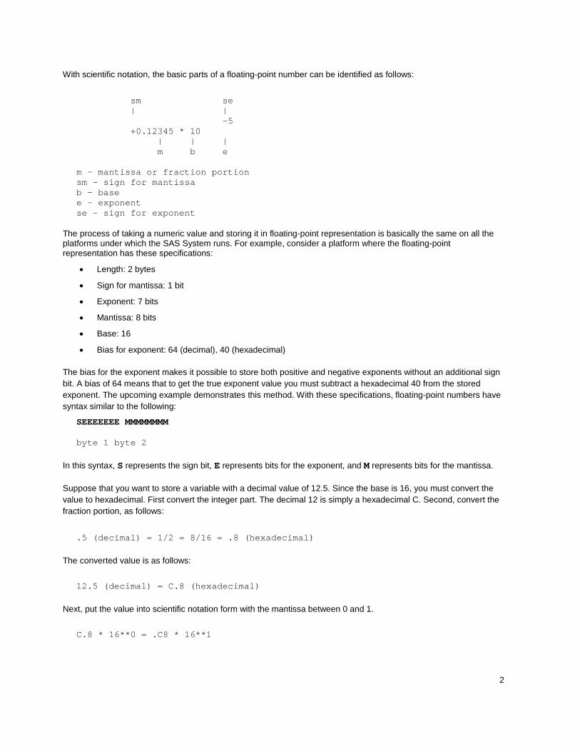
With scientific notation, the basic parts of a floating-point number can be identified as follows:

sm se | | -5 +0.12345 * 10 | | | m b e m - mantissa or fraction portion sm - sign for mantissa b - base e - exponent se - sign for exponent

The process of taking a numeric value and storing it in floating-point representation is basically the same on all the platforms under which the SAS System runs. For example, consider a platform where the floating-point representation has these specifications:

Length: 2 bytes

Sign for mantissa: 1 bit

Exponent: 7 bits

Mantissa: 8 bits

Base: 16

Bias for exponent: 64 (decimal), 40 (hexadecimal)

The bias for the exponent makes it possible to store both positive and negative exponents without an additional sign bit. A bias of 64 means that to get the true exponent value you must subtract a hexadecimal 40 from the stored exponent. The upcoming example demonstrates this method. With these specifications, floating-point numbers have syntax similar to the following:

SEEEEEEE MMMMMMMM byte 1 byte 2

In this syntax, S represents the sign bit, E represents bits for the exponent, and M represents bits for the mantissa.

Suppose that you want to store a variable with a decimal value of 12.5. Since the base is 16, you must convert the value to hexadecimal. First convert the integer part. The decimal 12 is simply a hexadecimal C. Second, convert the fraction portion, as follows:

.5 (decimal) = 1/2 = 8/16 = .8 (hexadecimal)

The converted value is as follows:

12.5 (decimal) = C.8 (hexadecimal)

Next, put the value into scientific notation form with the mantissa between 0 and 1.

C.8 * 16**0 = .C8 * 16**1

3

The exponent for the value is 1. To determine the actual exponent that will be stored, take the exponent value and add the bias to it.

True Exponent + Bias = 1 + 40 = 41 = Stored Exponent

The final portion that is to be determined is the sign of the mantissa. By convention, the sign bit for positive mantissas is 0, and the sign bit for negative mantissas is 1.

The stored value now looks like this:

01000001 11001000 (binary) -or- 41 C8 (hexadecimal)

Different host computers can have different specifications for floating-point representation. All platforms on which the SAS System runs use 8 bytes for floating-point numbers. The number of bits allotted to the exponent and the base that is chosen for the exponent determines the range of magnitude that the system can accommodate. After the exponent bits have been allotted, one more bit is designated for the sign of the mantissa. The remaining bits are used for the mantissa, and they determine the precision that is available.

Now that you know how numbers are stored, you can understand how floating-point representation can introduce error. Integers up to a certain magnitude can be represented exactly. After a certain magnitude, the number of digits exceeds the precision of the mantissa. At this point, specific integers occur which cannot be represented. To determine the highest integer such that all integers between it and its negative can be represented exactly, use the following formula:

max_int = base ** max_num_digits

In this formula, MAX_NUM_DIGITS specifies the maximum number of digits that are available in the mantissa for the base that you are using. To illustrate this concept, apply the following formula to the specifications listed earlier.

max_int = base ** max_num_digits = 16 ** 2 = 256

To see how this value is stored, convert it as follows:

256 (decimal) = 100 * 16**0 (hexadecimal) = .100 * 16**3 = 4310

Above this value, there are some integers that require more digits for their representation than the mantissa has available. An example is the decimal number 257. This example uses specifications shown earlier:


Because there is room for only two hexadecimal digits in the mantissa, a convention must be adopted as to how to handle the third (and all subsequent) digits. One convention is to truncate the value at the length that can be stored. This is the convention that is used in this paper. Another alternative is to round the value based on the digits that cannot be stored. Although it can be argued that one convention is better than the other, neither convention results in an exact representation of the value.

Although there is a maximum integer that can be stored confidently, this does not mean that all integers above this value cannot be represented, as shown in this example:


4

Like integers, some fractions can be represented exactly. However, there are also a number of fractions that cannot be represented. Unlike integers, the magnitude does not determine whether the number can be represented. There are many examples of fractional values that cannot be represented even though they are not considered an extreme magnitude. As a consequence, you are more likely to run into representation problems when you work with fractional values. To demonstrate this, use the representation specified earlier. A fractional value that can be represented exactly is .5 (decimal).

.5 (decimal) = .8 * 16**0 (hexadecimal) = 4080

However, consider a value such as .1 (decimal). After the experience with integers, your first guess might be that this value can also be represented exactly, since it is the same magnitude as .5 (decimal). However, the value .1 (decimal) cannot be represented in hexadecimal; it results in an infinite series. The conversion is as follows:

.1 (decimal) = .199999... * 16**0 (hexadecimal) = 4019

Like the integer 257 (decimal) above, there are more hexadecimal digits than you have room for in the mantissa. The digits that you do not have room for are truncated. A similar problem occurs when you attempt to represent the fraction 1/3 in decimal representation. The decimal representation of the fraction 1/3 results in the infinite series of .333333... An infinite series can never be represented exactly in a finite numerical representation.

Why Use Floating-Point Representation? There are other representations that are used to store numbers on computers. Each of these representations has advantages and disadvantages. Because the SAS System can be used for a wide variety of applications, a good general- purpose representation is needed. Floating-point representation provides the best compromise between precision and magnitude. It is also the most flexible of the methods that are available. Here is an overview of alternative methods:

Integer: Obviously this method is not sufficient as a general-purpose numeric representation because it cannot accommodate fractional values. The maximum space that is available for an integer on most hardware platforms is a full word (4 bytes or 32 bits). Because the 32 bits that are used for an integer is less than the mantissa for all systems, all numbers that can be stored in an integer can also be stored in floating-point representation.

Decimal or packed decimal: The decimal method is a better choice than integer as a general-purpose representation. One advantage to this method is that fractional values can be stored in a decimal representation. Because no explicit decimal point is stored in the representation, the application must be written to keep up with the decimal point. Another advantage is that within its range, decimal representation can store decimal numbers exactly. Values that cannot be represented as decimal numbers will have the same representation problem as what occurs with floating-point representation. Hardware platforms that allow decimal representation limits it to a maximum of 16 bytes in length. This length enables representation for up to 31 digits. Decimal representation does not have a separate exponent and mantissa. This means that for any particular value to be stored, there is a tradeoff between magnitude and precision. To demonstrate this, consider the following specifications for a packed decimal representation.

o Length: 3 bytes

o Sign: 1/2 byte

o Number of digits: 5

This representation has the following syntax:

DD DD DS bytes - 1 2 3

5

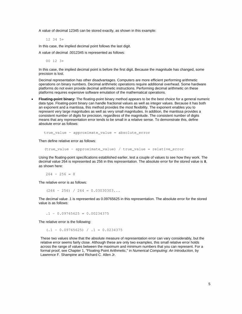
A value of decimal 12345 can be stored exactly, as shown in this example:

12 34 5+

In this case, the implied decimal point follows the last digit.

A value of decimal .0012345 is represented as follows:

00 12 3+ In this case, the implied decimal point is before the first digit. Because the magnitude has changed, some precision is lost.

Decimal representation has other disadvantages. Computers are more efficient performing arithmetic operations on binary numbers. Decimal arithmetic operations require additional overhead. Some hardware platforms do not even provide decimal arithmetic instructions. Performing decimal arithmetic on these platforms requires expensive software emulation of the mathematical operations.

Floating-point binary: The floating-point binary method appears to be the best choice for a general numeric data type. Floating-point binary can handle fractional values as well as integer values. Because it has both an exponent and a mantissa, this method provides the most flexibility. The exponent enables you to represent very large magnitudes as well as very small magnitudes. In addition, the mantissa provides a consistent number of digits for precision, regardless of the magnitude. The consistent number of digits means that any representation error tends to be small in a relative sense. To demonstrate this, define absolute error as follows:

true_value - approximate_value = absolute_error

Then define relative error as follows:

(true_value - approximate_value) / true_value = relative_error Using the floating-point specifications established earlier, test a couple of values to see how they work. The decimal value 264 is represented as 256 in this representation. The absolute error for the stored value is 8, as shown here:

264 - 256 = 8 The relative error is as follows:

(264 - 256) / 264 = 0.03030303... The decimal value .1 is represented as 0.09765625 in this representation. The absolute error for the stored value is as follows:

.1 - 0.09765625 = 0.00234375

The relative error is the following:

(.1 - 0.09765625) / .1 = 0.0234375 These two values show that the absolute measure of representation error can vary considerably, but the relative error seems fairly close. Although these are only two examples, this small relative error holds across the range of values between the maximum and minimum numbers that you can represent. For a formal proof, see Chapter 1, "Floating Point Arithmetic," in Numerical Computing: An Introduction, by Lawrence F. Shampine and Richard C. Allen Jr.

6

When is Representation Error a Problem?

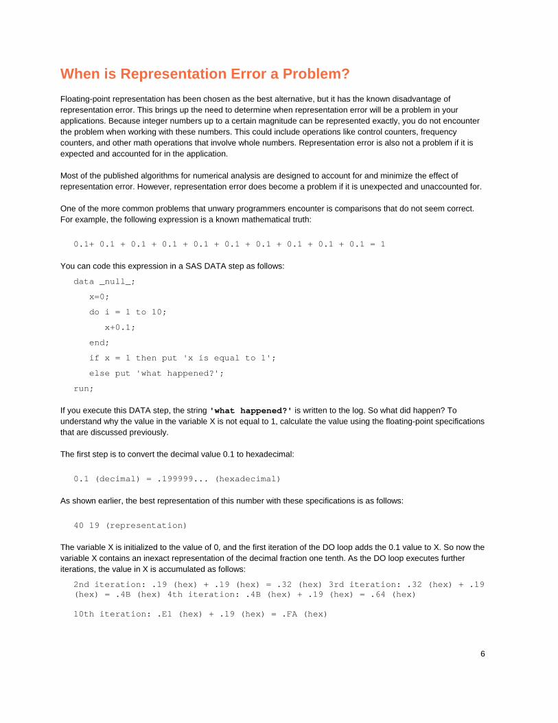
Floating-point representation has been chosen as the best alternative, but it has the known disadvantage of representation error. This brings up the need to determine when representation error will be a problem in your applications. Because integer numbers up to a certain magnitude can be represented exactly, you do not encounter the problem when working with these numbers. This could include operations like control counters, frequency counters, and other math operations that involve whole numbers. Representation error is also not a problem if it is expected and accounted for in the application.

Most of the published algorithms for numerical analysis are designed to account for and minimize the effect of representation error. However, representation error does become a problem if it is unexpected and unaccounted for.

One of the more common problems that unwary programmers encounter is comparisons that do not seem correct. For example, the following expression is a known mathematical truth:

0.1+ 0.1 + 0.1 + 0.1 + 0.1 + 0.1 + 0.1 + 0.1 + 0.1 + 0.1 = 1

You can code this expression in a SAS DATA step as follows:

data _null_;

x=0;

do i = 1 to 10;

x+0.1;

end;

if x = 1 then put 'x is equal to 1';

else put 'what happened?';

run;

If you execute this DATA step, the string 'what happened?' is written to the log. So what did happen? To understand why the value in the variable X is not equal to 1, calculate the value using the floating-point specifications that are discussed previously.

The first step is to convert the decimal value 0.1 to hexadecimal:

0.1 (decimal) = .199999... (hexadecimal)

As shown earlier, the best representation of this number with these specifications is as follows:

40 19 (representation)

The variable X is initialized to the value of 0, and the first iteration of the DO loop adds the 0.1 value to X. So now the variable X contains an inexact representation of the decimal fraction one tenth. As the DO loop executes further iterations, the value in X is accumulated as follows:

2nd iteration: .19 (hex) + .19 (hex) = .32 (hex) 3rd iteration: .32 (hex) + .19 (hex) = .4B (hex) 4th iteration: .4B (hex) + .19 (hex) = .64 (hex) 10th iteration: .E1 (hex) + .19 (hex) = .FA (hex)

7

This yields the following representation in the variable X after the final iteration of the DO loop:

40 FA (representation)

Finally, compare the value in the variable X to the constant value 1, and see that the two are indeed not equal.

40 FA ^= 41 10

In fact, the values differ by .06 (hexadecimal). This example also demonstrates how representation error can propagate through expressions and produce inaccurate results.

If representation error is not accounted for, the error can propagate and reduce the number of significant digits to an unacceptable level. Error propagation is not merely the sum of representation error for each component of an equation, but may turn out to exaggerate the representation error. For a further discussion, see Chapter 16, "Propagation of Rounding Error," in Elements of Numerical Analysis by Peter Henrici.

Another Type of Error: Loss of Significance

Another factor that might affect your calculations is loss of significance. Loss of significance is not directly related to representation error, but it is a subject that will also be of interest as you investigate numeric representation in your applications. If a representation has finite limits, there are only a finite number of significant digits available with that representation. You must construct equations carefully to preserve the available significant digits. Usually, this loss of significance occurs when the magnitudes of values vary greatly during a calculation. This scenario can be demonstrated easily with the earlier floating-point specifications because the mantissa was defined large enough for only two hexadecimal digits. Consider the following expression that evaluates to a decimal value of 288:

255 + 20 + 13 (all values in decimal)

Now convert the values to their floating-point representation.

42 FF + 42 14 + 41 D0

Adding the first two values produces the following results:

42 FF + 42 14 = 43 11 3 = 43 11 (representation)

The result of the addition needs three digits to be represented exactly. Because only two digits are available, some significance is lost in the representation. Add this result to the third value to get the final result.

43 11 + 41 D0 = 43 11 D = 43 11 (representation)

The same loss of significance occurs again. The final value is a decimal 272, not the expected 288. However, changing the order in which the expression is evaluated, can produce the correct results.

42 FF + ( 42 14 + 41 D0 ) = 42 FF + 42 21 = 43 12 = 288 (decimal)

The fact that results of the expression changes as you reorder the operands can be disturbing. It appears that a fundamental mathematical law, the associative law, is breaking down. The associative law states the following:

(x + y) + z = x + (y + z)

8

The previous example shows that reliance on the associative law breaks down when loss of significance can occur. For further information about this topic, see section 4.2.2, "Accuracy of Floating Point Arithmetic," in The Art of Computer Programming by Donald E. Knuth.

Knowing What You Really Have

Now that you know some of the issues involved with numeric representation, consider how these issues apply to SAS application programming.

As stated earlier, all SAS numeric variables are stored as floating-point binary numbers. Rarely, though, does the programmer display numeric values as such. Usually, numeric values are printed using a SAS format. This formatting makes the value more readable, but is it exactly what is stored in the variable? In many cases, it is not.

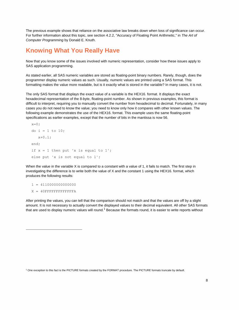
The only SAS format that displays the exact value of a variable is the HEX16. format. It displays the exact hexadecimal representation of the 8-byte, floating-point number. As shown in previous examples, this format is difficult to interpret, requiring you to manually convert the number from hexadecimal to decimal. Fortunately, in many cases you do not need to know the value; you need to know only how it compares with other known values. The following example demonstrates the use of the HEX16. format. This example uses the same floating-point specifications as earlier examples, except that the number of bits in the mantissa is now 56.

x=0;

do i = 1 to 10;

x+0.1;

end;


else put 'x is not equal to 1';

When the value in the variable X is compared to a constant with a value of 1, it fails to match. The first step in investigating the difference is to write both the value of X and the constant 1 using the HEX16. format, which produces the following results:

1 = 4110000000000000

X = 40FFFFFFFFFFFFFA

After printing the values, you can tell that the comparison should not match and that the values are off by a slight amount. It is not necessary to actually convert the displayed values to their decimal equivalent. All other SAS formats that are used to display numeric values will round.1 Because the formats round, it is easier to write reports without

1 One exception to this fact is the PICTURE formats created by the FORMAT procedure. The PICTURE formats truncate by default.

9

having to worry about representation error. If you are trying to determine the exact value of a variable, the rounding can become an obstacle. In the previous example, you can write the two values using the standard numeric format of 32.30:

1 = 1.000000000000000000000000000000

X = 1.000000000000000000000000000000

This format appears to display many significant digits, but there is still no difference in the values. In fact, however, the format is actually rounding the value in the variable X to display it as 1.

Handling the Problem Once you understand the basics of numeric representation and can recognize when it is causing a problem, you can begin to discover ways of handling the problem. Unfortunately, there is no one method that best handles the problems that are caused by numeric representation error. What is a perfectly good solution for one application might drastically affect the performance and results of another application. There is usually one method, however, that is most appropriate for each application. Earlier in this article, situations were defined in which numeric representation error is not a problem. If you have an application that is encountering a problem with representation error, the key is to transform the problematic area of the application into a situation where the error is not a problem. To do this, you can either avoid the problem or manage it where it occurs. You can avoid the problem by using integers for the numeric values so that they can be represented exactly.

There are also ways that you can account for representation error in your application. One method is to round your numeric values at various points in the application. Another method is to introduce some type of fuzz factor when doing numeric comparisons that might be exposed to representation error. The following sections describe some of these methods in more detail.

Using Integers to Represent Numeric Values Exactly

At first glance, using integers does not appear to be a viable alternative for many applications. Further investigation however, reveals that this alternative might actually cover a larger number of applications. The key to this method is to store the entire numeric value as an integer. If values are integers to start with, it is easy, but even in cases where you must begin with fractions (for example, in financial applications), using this method might still be possible. Such applications frequently store values as dollars, with the cents portion stored as a fraction. Instead of storing values this way, you can store the values as cents, thereby storing the entire value as an integer. Here are some examples of how values are stored:

Value Stored As ----- --------- 25› 25 $5 500

Once the values are stored as integers, the expressions in the application can be written to work with the integer values. You would perform integer arithmetic in the expressions, and as long as you do not exceed the maximum continuous integer value (see above for calculating this), all of the values are represented exactly.

One potential problem with using this method is reading the values into SAS variables as integers. If values are entered manually, they can be entered as integers. If you read them from an external file using an implicit decimal point, you can adjust the decimal specification in the informat to read the values as integers. An example of this is the PD. informat for packed decimal fields. If you had previously used the PD4.2 informat to read a value from a field, the value would have up to five decimal digits in front of the decimal point and two after the decimal point. Because there is not an explicit decimal point stored in packed decimal fields, you can read the number as an integer by using the PD4. informat.

10

If the field in the external file has an explicit decimal point, you might be able to read the value as an integer using the COMMAX. informat. The primary use of the COMMAX. informat is to read values in the same manner as the COMMA. informat, except that it exchanges the normal roles of the comma and decimal point. As a consequence, any embedded decimal points are ignored. Note that you cannot use the COMMAX. informat if the field also contains embedded commas.

If none of the above options work for your data, you can multiply by a scale factor to shift the fraction to the integer portion. You can then apply the INT function to remove any representation error that is introduced by the fraction.

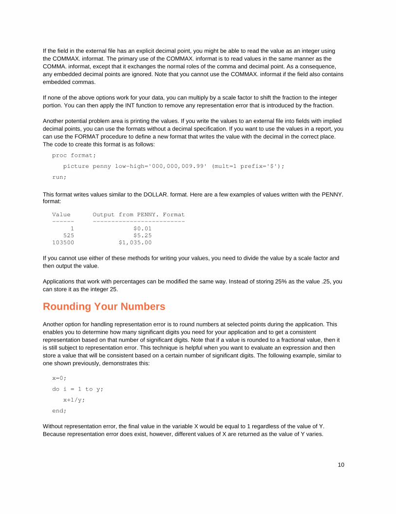
Another potential problem area is printing the values. If you write the values to an external file into fields with implied decimal points, you can use the formats without a decimal specification. If you want to use the values in a report, you can use the FORMAT procedure to define a new format that writes the value with the decimal in the correct place. The code to create this format is as follows:

proc format;

picture penny low-high='000,000,009.99' (mult=1 prefix='$');

run;

This format writes values similar to the DOLLAR. format. Here are a few examples of values written with the PENNY. format:

Value Output from PENNY. Format ------ ------------------------- 1 $0.01 525 $5.25 103500 $1,035.00

If you cannot use either of these methods for writing your values, you need to divide the value by a scale factor and then output the value.

Applications that work with percentages can be modified the same way. Instead of storing 25% as the value .25, you can store it as the integer 25.

Rounding Your Numbers

Another option for handling representation error is to round numbers at selected points during the application. This enables you to determine how many significant digits you need for your application and to get a consistent representation based on that number of significant digits. Note that if a value is rounded to a fractional value, then it is still subject to representation error. This technique is helpful when you want to evaluate an expression and then store a value that will be consistent based on a certain number of significant digits. The following example, similar to one shown previously, demonstrates this:

x=0;

do i = 1 to y;

x+1/y;

end;

Without representation error, the final value in the variable X would be equal to 1 regardless of the value of Y. Because representation error does exist, however, different values of X are returned as the value of Y varies.

11

The result requires only one significant digit, so you can round the number to one significant digit to get a consistent result. Modify the example as follows:

x=0;

do i = 1 to y;

x+1/y;

end;

x=round(x, 1);

The result is then rounded to one significant digit, and the result is consistent, regardless of the value of Y. Notice that the 1 in the second argument to the ROUND function specifies that the value is rounded to the nearest integer. It is only by coincidence that the values are also rounding to one significant digit.

Most SAS applications obtain acceptable results from the SAS ROUND function. If your applications need more control over rounding than is provided for in the ROUND function, you must define your own rounding routine to be used instead of the SAS ROUND function.

The key to defining your own rounding routine is to determine how much of a fuzz factor should be added. You want to add enough of a fuzz factor so that values that should be rounded up are indeed rounded up, but you do not want to such a large fuzz factor that values that should be rounded down are rounded up instead. If the only error that will be present in your values is representation error, then you need to add only a binary 1 in the least significant bit of the representation. First, you must determine what the actual value of the fuzz factor should be. Although the least significant bit is always the last bit in the representation, the value it represents changes based on the magnitude of the number being represented. For example, the following is a representation of the decimal value 256.115 using the floating-point specifications that contains 56 bits in the mantissa:

256.115 (decimal) = 4310 01D7 0A3D 70A3 (representation)

The fuzz factor for this value needs to have the same exponent and the least significant bit set to 1. This value is as follows:

fuzz_factor = 4300 0000 0000 0001 = 1*16**-11 (decimal)

This is the smallest fuzz factor that can be added to 256.115 and its significance not be lost. Now that the fuzz factor has been determined, you can add it to the variable value. The result is that the value that will be rounded. The following DATA step illustrates how you can add the fuzz factor:

data _null_;

fuzz = 1*16**-11;

x=256.115;

y=round(x+fuzz, .01);

put _all_;

run;

The fuzz factor used in this example is a constant value. Using a constant fuzz factor is fine as long as the values to be rounded are all of the same magnitude. Because this fuzz factor is dependent on the exponent, the fuzz factor needs to be adjusted if the exponent of the value changes. Suppose the value to be fuzzed is 4096.115 (decimal).

4096.115 (decimal) = 4410 001D 70A3 D70A (representation)

12

This value has a larger magnitude than the previous value. The fuzz factor for this value is as follows: fuzz_factor = 4400 0000 0000 0001 = 1*16**-10 (decimal)

If your application uses values with different magnitudes, you might need to calculate the fuzz factor for each value based on the value's magnitude. You can determine the magnitude of a value with the LOG function. Once the magnitude is determined, you can calculate an appropriate fuzz factor and add it to the variable value. See the appendix for an example of a macro that implements this technique.

The fuzz factors calculated previously are sufficient to handle any representation error that might be present in a value. But, what if the value is not rounding correctly because of a loss of significance? If there is error caused by loss of significance, it is also necessary to add a fuzz factor to cause values to round correctly. In this situation, the fuzz factor is based on the number of significant digits as well as the magnitude of the value. Use the fuzz factor calculated for representation error as a starting point. For a decimal value of 4096.115, the fuzz factor is as follows:

4096.115 (decimal) = 4410 001D 70A3 D70A (representation) fuzz_factor = 4400 0000 0000 0001 = 1*16**-10 (decimal)

You now have a fuzz factor that is based on the magnitude of the value that you are rounding. If you think that the last two digits are not significant, you can increase the magnitude of the fuzz factor by two digits, as shown below:

fuzz_factor = 4400 0000 0000 0001 = 1*16**-10 (decimal) new_fuzz_factor = 4400 0000 0000 0100 = 1*16**-8 (decimal)

Only increase the fuzz factor enough to handle the expected loss of significance. If the fuzz factor is too large, you will begin to round up values incorrectly.

Once you decide to use rounding in your application to handle representation error, the next question is at what point in the application should you do the rounding? This requires careful consideration because rounding can reduce the number of significant digits. A simple rule is to round at the point where representation causes a problem.

Consider this example, which was shown previously:

x=0;

do i = 1 to y;

x+1/y;

end;

In this case, it is not necessary to round the intermediate values in the variable X. There were no problems in the application until the final result proved to be unexpected. Rounding the final number produced the correct results. If your application has trouble with a comparison operation because of representation, you should round during the comparison to correct the problem. If your problem is with representation error of intermediate values in an accumulation, then you can round while accumulating.

Fuzzing Your Comparisons

Another aspect you need to consider in your application is comparisons. Comparisons are significantly affected by representation error. When you use the EQUAL operator in a comparison, the operands must be exactly equal for the comparison to be true. This makes the operator almost useless for comparing numeric operands where there might be some degree of representation error. Most of the time when you do these comparisons, you want the expression to be true when the values are the same, but that does not mean they have to be exactly equal. There are times when the values are close enough that they should be considered the same, even though they are not exactly equal. One way of achieving this goal is to round one or both of the operands in the comparison. An

13

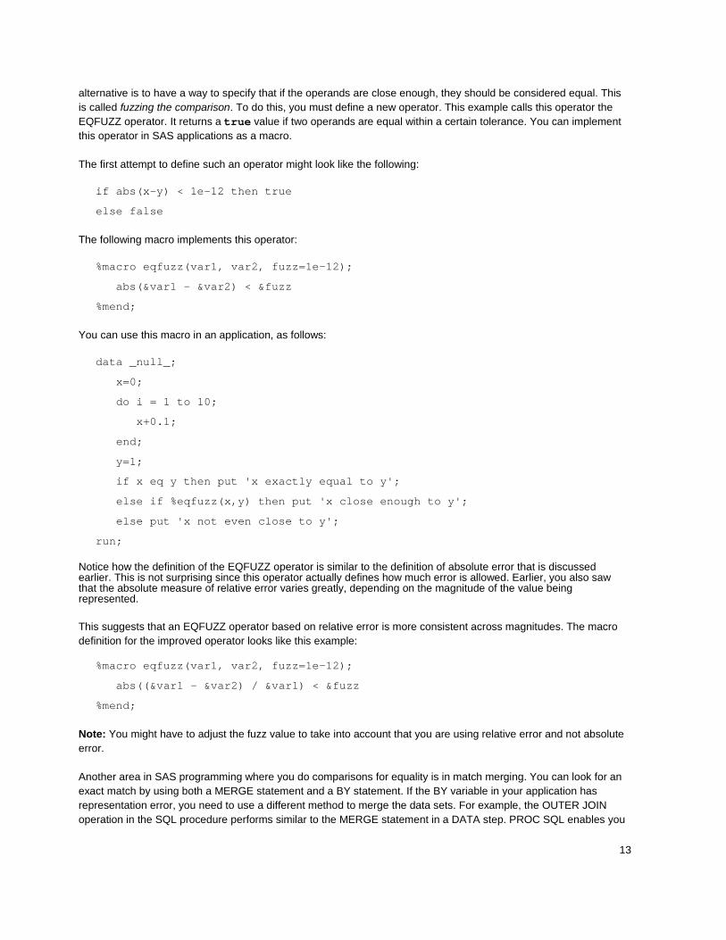
alternative is to have a way to specify that if the operands are close enough, they should be considered equal. This is called fuzzing the comparison. To do this, you must define a new operator. This example calls this operator the EQFUZZ operator. It returns a true value if two operands are equal within a certain tolerance. You can implement this operator in SAS applications as a macro.

The first attempt to define such an operator might look like the following:

if abs(x-y) < 1e-12 then true

else false

The following macro implements this operator:

%macro eqfuzz(var1, var2, fuzz=1e-12);

abs(&var1 - &var2) < &fuzz

%mend;

You can use this macro in an application, as follows:

data _null_;

x=0;

do i = 1 to 10;

x+0.1;

end;

y=1;

if x eq y then put 'x exactly equal to y';

else if %eqfuzz(x,y) then put 'x close enough to y';

else put 'x not even close to y';

run;

Notice how the definition of the EQFUZZ operator is similar to the definition of absolute error that is discussed earlier. This is not surprising since this operator actually defines how much error is allowed. Earlier, you also saw that the absolute measure of relative error varies greatly, depending on the magnitude of the value being represented.

This suggests that an EQFUZZ operator based on relative error is more consistent across magnitudes. The macro definition for the improved operator looks like this example:


abs((&var1 - &var2) / &var1) < &fuzz

%mend;

Note: You might have to adjust the fuzz value to take into account that you are using relative error and not absolute error.

Another area in SAS programming where you do comparisons for equality is in match merging. You can look for an exact match by using both a MERGE statement and a BY statement. If the BY variable in your application has representation error, you need to use a different method to merge the data sets. For example, the OUTER JOIN operation in the SQL procedure performs similar to the MERGE statement in a DATA step. PROC SQL enables you

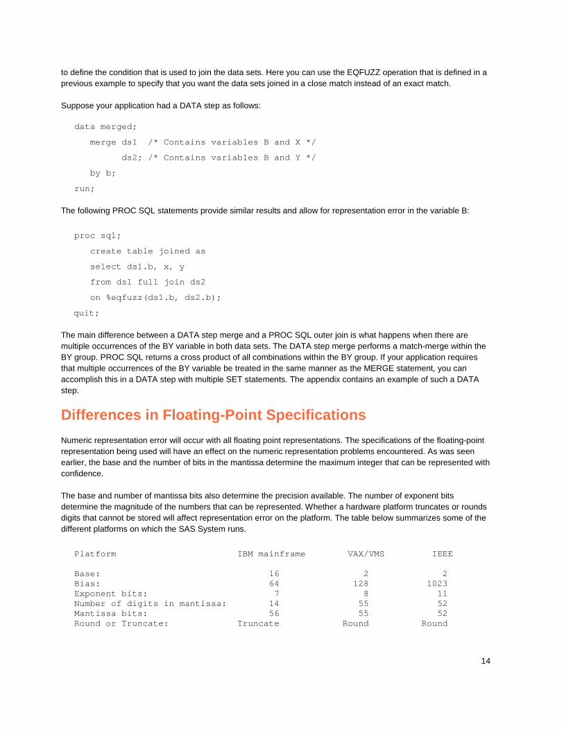
14

to define the condition that is used to join the data sets. Here you can use the EQFUZZ operation that is defined in a previous example to specify that you want the data sets joined in a close match instead of an exact match.

Suppose your application had a DATA step as follows:

data merged;

merge ds1 /* Contains variables B and X */

ds2; /* Contains variables B and Y */

by b;

run;

The following PROC SQL statements provide similar results and allow for representation error in the variable B:

proc sql;

create table joined as

select ds1.b, x, y

from ds1 full join ds2

on %eqfuzz(ds1.b, ds2.b);

quit;

The main difference between a DATA step merge and a PROC SQL outer join is what happens when there are multiple occurrences of the BY variable in both data sets. The DATA step merge performs a match-merge within the BY group. PROC SQL returns a cross product of all combinations within the BY group. If your application requires that multiple occurrences of the BY variable be treated in the same manner as the MERGE statement, you can accomplish this in a DATA step with multiple SET statements. The appendix contains an example of such a DATA step.

Differences in Floating-Point Specifications

Numeric representation error will occur with all floating point representations. The specifications of the floating-point representation being used will have an effect on the numeric representation problems encountered. As was seen earlier, the base and the number of bits in the mantissa determine the maximum integer that can be represented with confidence.

The base and number of mantissa bits also determine the precision available. The number of exponent bits determine the magnitude of the numbers that can be represented. Whether a hardware platform truncates or rounds digits that cannot be stored will affect representation error on the platform. The table below summarizes some of the different platforms on which the SAS System runs.

Platform IBM mainframe VAX/VMS IEEE Base: 16 2 2 Bias: 64 128 1023 Exponent bits: 7 8 11 Number of digits in mantissa: 14 55 52 Mantissa bits: 56 55 52 Round or Truncate: Truncate Round Round

15

IBM mainframe platforms include the MVS and z/OS operating systems. The IEEE standard is used by the Windows and UNIX operating systems. Any programmer working with a variety of hardware might see slightly different results from one machine to the next.

For a detailed discussion on the different floating point representations used by the platforms on which the SAS system runs, see the section "Numeric Precision in SAS Software”, in the SAS® 9.4 Language Reference: Concepts. Additional information can be found in the SAS Global Forum paper "Numeric Precision Considerations in SAS Software" by Richard D. Langston.

The SAS LENGTH statement will also have an effect on the numeric representations in SAS applications. The LENGTH statement can be used to reduce the number of bytes needed to store numeric variables in SAS data sets. It does this by reducing the number of bits in the mantissa of the representation. This reduces the precision available. The length of variables containing integer values can be reduced as long as there are enough bits in the mantissa to store each value exactly. For variables that contain fractional values, the reduced length will most likely increase the problem of representation error. For this reason, you should not decrease the length of numeric variables, which might contain fractional values, from the default length of 8 bytes.

Conclusion

By using a floating-point binary representation to store numbers, you become vulnerable to representation error. Other numeric representations might not have the same problems with representation that floating point has, but they have other limitations that make them less than desirable for general purpose use. In most cases, the representation error that might be present in a floating point number will not cause a problem to the SAS application programmer. If you recognize that representation error might affect an application, you can take steps to account for representation error and eliminate unexpected results.

Acknowledgments

The author would like to acknowledge Thomas Zack for his contributions in research for this article.

References

Henrici, P. 1964. Elements of Numerical Analysis, New York: John Wiley & Sons, Inc.

Knuth, D.E., 1981. The Art of Computer Programming, Volume 2, Seminumerical Algorithms, Reading MA: Addison-Wesley.

Langston, R.D. 1987. "Numeric Precision Considerations in SAS Software", Proceedings of the Twelfth Annual SAS Users Group International Conference, Cary, NC: SAS Institute Inc. Available at www.sascommunity.org/sugi/SUGI87/Sugi-12-118%20Langston.pdf.

SAS Institute Inc., 2013. SAS® 9.4 Language: Reference: Concepts, Second Edition, Cary, NC: SAS Institute Inc. Available at support.sas.com/documentation/cdl/en/lrcon/67227/PDF/default/lrcon.pdf.

Shampine, L.F. and Allen, Jr. 1973. Numerical Computing: an introduction, Philadelphia, PA: W.B. Saunders Company.

http://www.sascommunity.org/sugi/SUGI87/Sugi-12-118%20Langston.pdf

http://support.sas.com/documentation/cdl/en/lrcon/67227/PDF/default/lrcon.pdf

16

Appendix

/**************************************************************************/ /* The following examples are provided to illustrate the concepts that */ /* are discussed in this article. */ /**************************************************************************/ /**************************************************************************/ /* The following DATA step is a typical example of unexpected results */ /* because of representation error. Notice the hex representations of the */ /* variable as it is accumulated. */ /**************************************************************************/

data _null_;

x=0;

do i = 1 to 10;

x+0.1;

put x= hex16. '(hex) ' x= '(formatted dec)';

end;


else put 'what happened?';

run;

/**************************************************************************/ /* This DATA step demonstrates how to calculate the maximum integer */ /* that can be represented with confidence. Set the BASE and MAX_DIGT */ /* variables based on the platform on which you are running. */ /**************************************************************************/

data _null_;

base = 16; /* 16 for IBM, 2 for VAX and IEEE */

max_digt = 14; /* 14 for IBM, 56 for VAX, 53 for IEEE */

/* Compute maximum integer and display */

max_int = base ** max_digt;

put @2 max_int= hex16. '(hex) ' max_int comma22. ' (dec)' ;

/************************************************************/

/* This DO loop attempts to store the five integers before */

/* and after the maximum. Notice how some of the integers */

/* after the maximum cannot be stored exactly. */

/************************************************************/

put / @2 'I' @8 'MAX_INT + I (in hex)' @31 'MAX_INT + I (in dec)'

/ @1 '---' @8 '--------------------' @31 '--------------------';

do i = -5 to 5;

x = max_int + i;

put @1 i 2. @10 x hex16. @30 x comma22.;

end;

run;

17

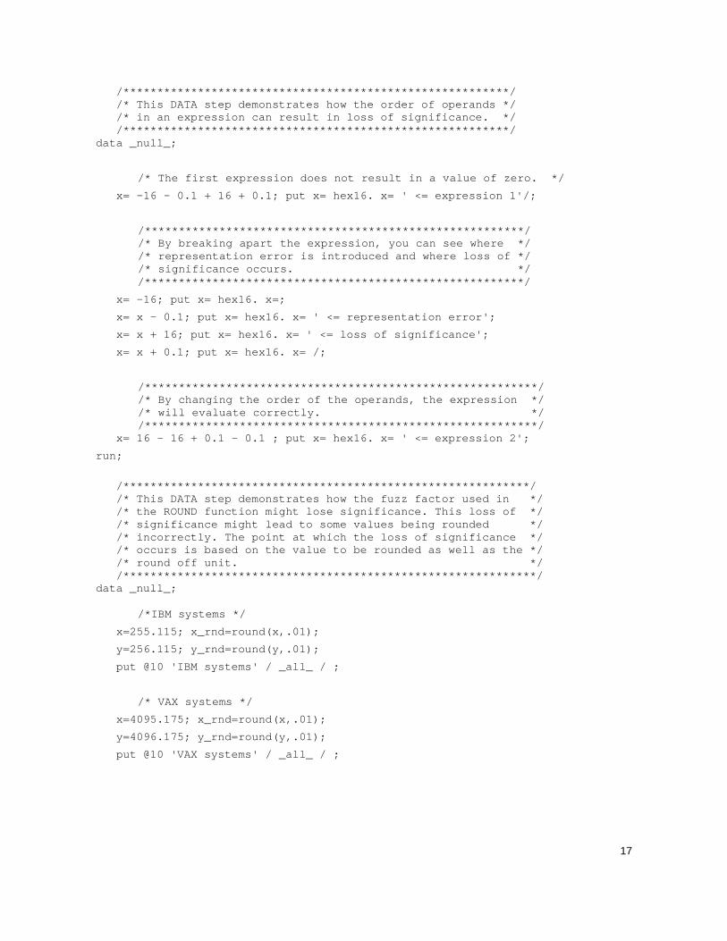
/*********************************************************/ /* This DATA step demonstrates how the order of operands */ /* in an expression can result in loss of significance. */ /*********************************************************/

data _null_;

/* The first expression does not result in a value of zero. */

x= -16 - 0.1 + 16 + 0.1; put x= hex16. x= ' <= expression 1'/;

/********************************************************/ /* By breaking apart the expression, you can see where */ /* representation error is introduced and where loss of */ /* significance occurs. */ /********************************************************/

x= -16; put x= hex16. x=;

x= x - 0.1; put x= hex16. x= ' <= representation error';

x= x + 16; put x= hex16. x= ' <= loss of significance';

x= x + 0.1; put x= hex16. x= /;

/**********************************************************/ /* By changing the order of the operands, the expression */ /* will evaluate correctly. */ /**********************************************************/

x= 16 - 16 + 0.1 - 0.1 ; put x= hex16. x= ' <= expression 2';

run;

/************************************************************/ /* This DATA step demonstrates how the fuzz factor used in */ /* the ROUND function might lose significance. This loss of */ /* significance might lead to some values being rounded */ /* incorrectly. The point at which the loss of significance */ /* occurs is based on the value to be rounded as well as the */ /* round off unit. */ /*************************************************************/

data _null_;

/*IBM systems */

x=255.115; x_rnd=round(x,.01);

y=256.115; y_rnd=round(y,.01);

put @10 'IBM systems' / _all_ / ;

/* VAX systems */

x=4095.175; x_rnd=round(x,.01);

y=4096.175; y_rnd=round(y,.01);

put @10 'VAX systems' / _all_ / ;

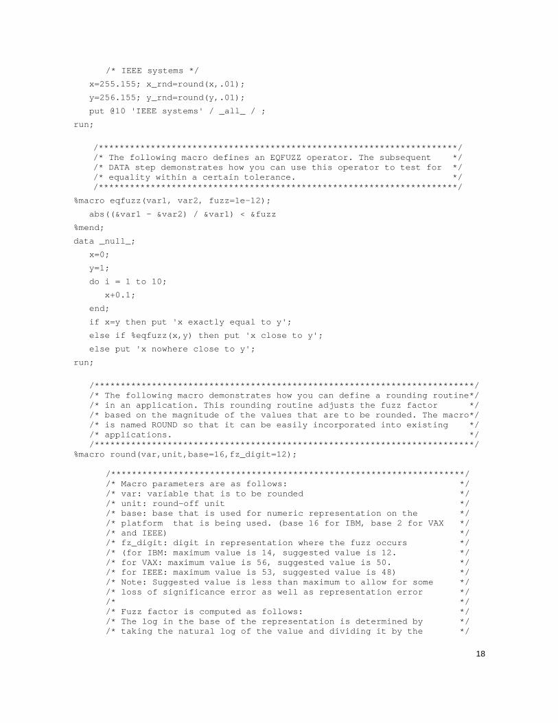
18

/* IEEE systems */

x=255.155; x_rnd=round(x,.01);

y=256.155; y_rnd=round(y,.01);

put @10 'IEEE systems' / _all_ / ;

run;

/*********************************************************************/ /* The following macro defines an EQFUZZ operator. The subsequent */ /* DATA step demonstrates how you can use this operator to test for */ /* equality within a certain tolerance. */ /*********************************************************************/


abs((&var1 - &var2) / &var1) < &fuzz

%mend;

data _null_;

x=0;

y=1;

do i = 1 to 10;

x+0.1;

end;

if x=y then put 'x exactly equal to y';

else if %eqfuzz(x,y) then put 'x close to y';

else put 'x nowhere close to y';

run;

/*************************************************************************/ /* The following macro demonstrates how you can define a rounding routine*/ /* in an application. This rounding routine adjusts the fuzz factor */ /* based on the magnitude of the values that are to be rounded. The macro*/ /* is named ROUND so that it can be easily incorporated into existing */ /* applications. */ /*************************************************************************/

%macro round(var,unit,base=16,fz_digit=12);

/********************************************************************/ /* Macro parameters are as follows: */ /* var: variable that is to be rounded */ /* unit: round-off unit */ /* base: base that is used for numeric representation on the */ /* platform that is being used. (base 16 for IBM, base 2 for VAX */ /* and IEEE) */ /* fz_digit: digit in representation where the fuzz occurs */ /* (for IBM: maximum value is 14, suggested value is 12. */ /* for VAX: maximum value is 56, suggested value is 50. */ /* for IEEE: maximum value is 53, suggested value is 48) */ /* Note: Suggested value is less than maximum to allow for some */ /* loss of significance error as well as representation error */ /* */ /* Fuzz factor is computed as follows: */ /* The log in the base of the representation is determined by */ /* taking the natural log of the value and dividing it by the */

19

/* natural log of the base. The resulting value is raised to the */ /* next integer to determine the magnitude of the value. The */ /* fz_digit parameter is subtracted from the magnitude of the value */ /* to determine the magnitude of the fuzz factor. The base is then */ /* raised to this magnitude and multiplied by the sign of the value */ /* to create the actual fuzz factor. This fuzz factor is added to the */ /* variable value and the ROUND function is called. */ /**********************************************************************/

round((&var+

(sign(&var)*

&base**(ceil(log(abs(&var))/log(&base))-&fz_digit))),

&unit)

%mend round;

/**********************************************************/ /* This DATA step demonstrates how the previously defined */ /* ROUND macro can be used in your application. */ /**********************************************************/

data _null_;

/* IBM systems */

x=255.115; x_rnd=%round(x,.01);

y=256.115; y_rnd=%round(y,.01);

put @10 'IBM systems' / _all_ / ;

/* VAX systems */

x=4095.175; x_rnd=%round(x,.01);

y=4096.175; y_rnd=%round(y,.01);

put @10 'VAX systems' / _all_ / ;

/* IEEE systems */

x=255.155; x_rnd=%round(x,.01);

y=256.155; y_rnd=%round(y,.01);

put @10 'IEEE systems' / _all_ / ;

run;

/**************************************************************************/ /* The following example demonstrates how you can write a DATA step with */ /* multiple SET statements that merge two data sets and allows for */ /* inexact matches in the BY variable. */ /**************************************************************************/ /**************************************************************************/ /* The following macro defines an EQFUZZ operator that checks for */ /* equality within a tolerance of 1E-3. */ /**************************************************************************/


abs(&var1 - &var2) <= &fuzz

%mend;

20

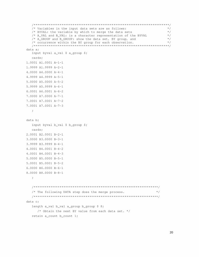
/*************************************************************************/ /* Variables in the input data sets are as follows: */ /* BYVAL: the variable by which to merge the data sets */ /* A_VAL and B_VAL: is a character representation of the BYVAL */ /* A_GROUP and B_GROUP: show the data set, BY group, and */ /* occurrence within the BY group for each observation. */ /*************************************************************************/

data a; input byval a_val $ a_group $;

cards;

1.0001 A1.0001 A-1-1

1.9999 A1.9999 A-2-1

4.0000 A4.0000 A-4-1

4.9999 A4.9999 A-5-1

5.0000 A5.0000 A-5-2

5.9999 A5.9999 A-6-1

6.0001 A6.0001 A-6-2

7.0000 A7.0000 A-7-1

7.0001 A7.0001 A-7-2

7.0001 A7.0001 A-7-3

;

data b;

input byval b_val $ b_group $;

cards;

2.0001 B2.0001 B-2-1

3.0000 B3.0000 B-3-1

3.9999 B3.9999 B-4-1

4.0001 B4.0001 B-4-2

4.0001 B4.0001 B-4-3

5.0000 B5.0000 B-5-1

5.0001 B5.0001 B-5-2

6.0000 B6.0000 B-6-1

8.0000 B8.0000 B-8-1

;

/*******************************************************************/

/* The following DATA step does the merge process. */

/*******************************************************************/

data c;

length a_val b_val a_group b_group $ 8;

/* Obtain the next BY value from each data set. */

retain a_count b_count 1;

21

if a_count <= a_nobs then

set a(keep=byval rename=(byval=next_a)) point=a_count nobs=a_nobs;

if b_count <= b_nobs then

set b(keep=byval rename=(byval=next_b)) point=b_count nobs=b_nobs;

/* Determine which data set needs to be advanced in order */

/* to merge the current by group. */

if %eqfuzz(next_a,next_b) then do;

read_a = 1;

read_b = 1;

end;

else if next_a < next_b then do;

read_a = 1;

read_b = 0; end; else do;

read_a = 0; read_b = 1;

end;

/* If the end of one of the data sets has been reached, then */

/* get the remaining observations from the other data set. */

if a_count > a_nobs then do;

read_a = 0;

read_b = 1;

end;

if b_count > b_nobs then do;

read_a = 1;

read_b = 0;

end;

/* Check for the beginning of a new BY group. */

if (read_a and not (%eqfuzz(next_a,byval))) or

(read_b and not (%eqfuzz(next_b,byval)))

then do;

/* reset variables to missing */ a_val = ' ';

b_val = ' ';

a_group = ' ';

b_group = ' ';

end;

22

/* Advance the data set and write the merged observation. */

if read_a then do;

set a;

a_count+1;

end;

if read_b then do;

set b;

b_count+1;

end;

drop next_a next_b read_a read_b;

run;

/**************************************************************************/ /* The following DATA steps demonstrate the results of a merge process */ /* if the BY values match exactly. */ /**************************************************************************/

data a2;

set a;

byval=round(byval);

data b2;

set b;

byval=round(byval);

data c2;

merge a2 b2;

by byval;

run;

/************************************************************************/ /* The following PROC SQL statements demonstrate how an outer join */ /* produces results similar to the DATA step MERGE statement. Notice */ /* how multiple occurrences of the BY variables are handled differently.*/ /************************************************************************/

proc sql;

create table d as

select a.byval, a_val, b_val, a_group, b_group

from a full join b

on %eqfuzz(a.byval,b.byval);

create table d2 as

select a2.byval, a_val, b_val, a_group, b_group

from a2 full join b2 on a2.byval = b2.byval;

quit;

To contact your local SAS office, please visit: sas.com/offices

SAS and all other SAS Institute Inc. product or service names are registered trademarks or trademarks of SAS Institute Inc. in the USA and other countries. ® indicates USA

registration. Other brand and product names are trademarks of their respective companies. Copyright © 2014, SAS Institute Inc. All rights reserved.

handling numeric representation errors in sas applications...numeric representation is a problem...

Documents