Handling the divergence constraints in Maxwell and

Vlasov-Maxwell simulations

Martin Campos Pinto, Marie Mounier, Eric Sonnendrucker

To cite this version:

Martin Campos Pinto, Marie Mounier, Eric Sonnendrucker. Handling the divergence con-straints in Maxwell and Vlasov-Maxwell simulations. 2015. <hal-01167456>

HAL Id: hal-01167456

https://hal.archives-ouvertes.fr/hal-01167456

Submitted on 24 Jun 2015

HAL is a multi-disciplinary open accessarchive for the deposit and dissemination of sci-entific research documents, whether they are pub-lished or not. The documents may come fromteaching and research institutions in France orabroad, or from public or private research centers.

L’archive ouverte pluridisciplinaire HAL, estdestinee au depot et a la diffusion de documentsscientifiques de niveau recherche, publies ou non,emanant des etablissements d’enseignement et derecherche francais ou etrangers, des laboratoirespublics ou prives.

Handling the divergence constraints in Maxwell and

Vlasov-Maxwell simulations

Martin Campos Pintoa,b, Marie Mounierc, Eric Sonnendruckerd,e

aCNRS, UMR 7598, Laboratoire Jacques-Louis Lions, F-75005, Paris, FrancebSorbonne Universites, UPMC Univ Paris 06, UMR 7598, Laboratoire Jacques-Louis

Lions, F-75005, Paris, FrancecNUCLETUDES, CS 70117, 91978 Courtaboeuf cedex, France

dMax-Planck Institute for plasma physics, Boltzmannstr. 2, D-85748 Garching, GermanyeMathematics Center, TU Munich, Boltzmannstr. 3, D-85747 Garching, Germany

Abstract

The aim of this paper is to review and classify the different methods thathave been developed to enable stable long time simulations of the Vlasov-Maxwell equations and the Maxwell equations with sources. These methodscan be classified in two types: field correction methods and sources correc-tion methods. The field correction methods introduce new unknowns in theequations, for which additional boundary conditions are in some cases nontrivial to find. The source correction consists in computing the sources sothat they satisfy a discrete continuity equation compatible with a discreteGauss’ law that needs to be defined in accordance with the discretization ofthe Maxwell propagation operator.

Keywords: Maxwell-Vlasov system, generalised Maxwell equations,discrete continuity equation, Particle in Cell (PIC) method

Corresponding author:Eric SonnendruckerMax-Planck Institute for plasma physicsBoltzmannstr. 2D-85748 GarchingGermanyemail: sonnen@ipp.mpg.dePhone: +49 89 32992070Fax: +49 89 32991011

Preprint submitted to Applied Mathematics and Computation June 11, 2015

1. Introduction

The collisionless evolution of the distribution of charged particles of aspecies s is governed by the relativistic Vlasov equation

∂fs∂t

+ vs(p) ·∇xfs + qs(E + v(p)×B) ·∇pfs = 0, (1)

where vs(p) = pmsγs

, the Lorentz factor being defined by γs =√

1 + p2

msc2

with c the speed of light. Macroscopic quantities relevant to the plasma areobtained as moments in p of the distribution function fs for each particlespecies. In particular the total charge and current densities are defined as

ρ =∑s

qs

∫fs(t,x,p) dp, J =

∑s

qs

∫vs(p)fs(t,x,p) dp. (2)

Integrating the Vlasov equation (1) over p and summing over the speciesyields the following continuity equation that will play a major role in thispaper:

∂ρ

∂t+ divJ = 0. (3)

The self-consistent electromagnetic fields E and B appearing in the Vlasovequation satisfy the following Maxwell equations in (0, T )× Ω,

∂E

∂t− c2 curlB = −J/ε0, (4)

∂B

∂t+ curlE = 0, (5)

divE = ρ/ε0, (6)

divB = 0, (7)

in addition to initial and boundary conditions. Taking the divergence of theAmpere equation (4) and using the Gauss law (6), we obtain ∂ρ

∂t+ divJ = 0

which means that the continuity equation (3) is a compatibility conditionfor Maxwell’s equations, those being ill-posed when the continuity equationis not satisfied. Moreover it can be shown that provided the divergenceconstraints (6)-(7) are satisfied at the initial time, they remain satisfied for

2

all times by the solution of Ampere (4) and Faraday (5), which have a uniquesolution by themselves provided adequate initial and boundary conditions.

At the continuous level, the continuity equation is thus a consequence ofthe Vlasov equation and all is fine for the Vlasov-Maxwell system. However,for a given discretization of the Vlasov-Maxwell system there is no reasonthat a discrete continuity equation holds, and that it should be compatiblewith the discrete Maxwell equations in a certain sense. Even though thisis generally the most acute problem in electromagnetic PIC simulations, insome cases problems can appear even without sources: the way in which theGauss laws (or divergence contraints) are satisfied needs to be compatiblewith the discrete Ampere and Faraday equations. Handling these compat-ibility issues is one way to solve the problem. Another is to modify theMaxwell equations, so that they are well posed independently of the sources,by introducing two additional scalar unknowns that can be seen as Lagrangemultipliers for the divergence constraints. These should become arbitrarilysmall when the continuity condition is close to being satisfied.

The aim of this paper is to review the different methods that have beenproposed in the literature and classify them in one of the two above cate-gories: using a structure preserving discretization with compatible discreteGauss laws and continuity equation or using a generalised set of Maxwellequations with additional unknowns that are easier to discretize. Indeed theinfinite dimensional kernel of the curl operator and the lack of compactnessof the inverse Maxwell operator has made it particularly hard to find gooddiscretization for Maxwell’s equations, especially for the eigenvalue problem[4, 5, 9, 14, 26]. Moreover, we will give an overview of classical and newtest cases that highlight our problem and the difficulties of the numericalmethods.

Although the compatibility problems of discrete Vlasov-Maxwell solvershas been widely discussed in the PIC literature it also exists for grid baseddiscretizations of the Vlasov equations and the same recipes apply there asdiscussed in [18, 39].

This article is organised as follows: In Section 2 we recall the classicalPIC algorithm and the generalised Maxwell equations in Section 3, whichcan be used to correct the fields. Section 4 is then devoted to presenting thestructure preserving methods in which the sources of Maxwell’s equations arecorrected. This will be discussed in the framework of finite differences, finiteelements and discontinuous Galerkin discretizations. Finally the problemand its solutions will be illustrated using different numerical test cases in

3

Section 5.

2. The Particle in Cell (PIC) method

The principle of a particle method is to approximate the distributionfunction f solution to the Vlasov equation by a sum of Dirac masses withweights wk and positions (xk(t),pk(t)) in phase space, 1 ≤ k ≤ N . Based onthese N macro-particles, the approximated distribution function then writes

fN(t,x,p) =N∑k=1

wkδ(x− xk(t)) δ(p− pk(t)).

Positions x0k, momenta p0

k and weights wk are initialised such that fN(0,x,p)is an approximation, in some sense, of the initial distribution function f0(x,v).The time evolution of the approximation is done by advancing the macro-particles along the characteristics of the Vlasov equation, i.e., by solving thesystem of differential equations

dxkdt

= v(pk)

dpkdt

= q(E(xk, t) + v(pk)×B)

with xk(0) = x0k, pk(0) = p0

k.

These differential equations are numerically solved by standard ODE solverslike the Runge-Kutta method or preferably a symplectic solver, given theHamiltonian structure of the equations. We shall not dwell on that as this isnot the central theme of the article.

To start the PIC algorithm, the initial distribution function is discretizedusing a Monte Carlo approach, i.e., the initial phase space positions of theparticles are drawn randomly using a pseudo-random or quasi-random num-ber generator according to the probability density associated to f0, whichis just f0 normalised so that its integral over phase space is one. As f0 ispositive this defines a probability density.

The particle approximation fN of the distribution function does not nat-urally give an expression for this function at all points of phase space. Thusfor the coupling with the field solver which is defined on the mesh a regu-larizing step is necessary. To this aim, a standard choice is to use a smoothconvolution kernel S which could typically be a Gaussian or preferably in

4

practice a smooth piecewise polynomial spline function which has the advan-tage of having a compact support. For a Finite Element discretization of thefield, the smoothing kernel is naturally provided by the Finite Element basisfunctions and no additional smoothing is required.

The sources for Maxwell’s equations ρ and J are then naturally definedfrom the numerical distribution function fN and the regularisation kernel S,for a particle species of charge q, by

ρS(t,x) = qN∑k=1

wkS(x− xk), JS(t,x) = qN∑k=1

wkS(x− xk)v(pk). (8)

This is obtained by direct discretization. When a structure preserving dis-cretization is needed, in this case a discrete continuity equation, some caremust be taken in the full discretization of the current as we shall see later.

With these ingredients the classical PIC loop can be performed at eachtime step:

1. Compute the fields at the particles positions.

2. Advance the phase space positions of the particles, by numerically in-tegrating the characteristics.

3. Compute the source for Maxwell’s equations, namely the current J andin some cases the charge density ρ.

4. Numerically solve Maxwell’s equations on a grid.

When a structure preserving method is used, special compatibility conditionsbetween steps 3 and 4 are necessary.

3. Generalised Maxwell’s equations: correcting the fields

Even though, provided the divergence constraints are satisfied at the ini-tial condition, they are satisfied at all times for the continuous Maxwell’sequations, this is not true for the classical PIC method when only Ampere(4) and Faraday’s equations (5) are numerically solved. This has been recog-nised early in the PIC literature and the first solution proposed by Boris [7],the so-called Boris correction, consists in correcting a posteriori, after eachfield solve, the electric field E into E = E + ∇ϕ such that ∇ · E = ρ/ε0.This yields the Poisson equation

−∆ϕ = ∇ ·E − ρ

ε0

.

5

In order to avoid a costly Poisson solve, Marder [31] proposed the followingcorrection of the electric field

En+1

= En+1 + ∆tgrad(ν(∇ ·En − ρn/ε0))

with ν a diffusion parameter chosen small enough for stability. This methodhas been further improved by Langdon [28]

En+1

= En+1 + ∆tgrad(ν(∇ ·En+1 − ρn+1/ε0))

which can also be seen as one Jacobi iteration for solving the Poisson equationproposed by Boris. A comparison of these methods is performed in [30].

These classical methods can all be interpreted as imposing the divergenceconstraint on the electric field by using a Lagrange multiplier using the fol-lowing generalised formulation of Maxwell’s equations introduced in [36]

∂tE− c2 curl B + c2∇p = − J

ε0,

∂tB + curl E = 0,

g(p) + div E =ρ

ε0,

div B = 0.

This implies ∂g(p)∂t− c2∆p = 1

ε0(∂ρ∂t

+ div J).A mathematical study of this system has been performed in [2]. The Boris

correction corresponds to the case g = 0, and the resulting Lagrange multi-plier p satisfies a Poisson equation with source ∂ρ

∂t+ divJ . The Marder and

Langdon corrections are equivalent to two different discretizations of theseequations with g(p) = p in which case p satisfies a heat equation transportingthe continuity error ∂ρ

∂t+ divJ out of the domain. It then becomes natural

to also consider the case g(p) = ∂tp in which case the Lagrange multipliersatisfies a wave equation and the generalised Maxwell’s equations becomehyperbolic and even strictly hyperbolic if a Lagrange multiplier is also usedfor the divB constraint. This set of generalised Maxwell’s equations reads

∂tE− c2 curl B + c2∇p = − J

ε0,

∂tB + curl E +∇p = 0,∂p

∂t+ div E =

ρ

ε0,

∂q

∂t+ div B = 0.

6

This is called the hyperbolic correction and was introduced in [35]. The erroris transported out of the domain fast enough to avoid accumulation. For this,absorbing boundary conditions are needed.

The idea has also been adapted for imposing the divB = 0 constraintin MHD by Dedner, Kemm, Kroner, Munz, Schnitzer and Wesenberg withconsiderable success [19].

The hyperbolic generalised Maxwell operator has a compact inverse whichcan be used to prove the existence and uniqueness of solutions [29], which isnot the case for the standard Maxwell’s equations. In this case the compact-ness of the evolution operator is guaranteed for divergence free functions.Hence the Gauss laws enforce that the solution remains in the correct do-main. This is what will need to be reproduced at the discrete level. For ageneralised formulation such a problem does not exist, which makes it robustfor any kind of consistent discretizations. However this comes at some ex-penses: First two new scalar unknowns are introduced and thus the systemto be solved becomes larger. Then these unknowns need boundary conditionswhich must be found according to the physics problem, which might not al-ways be easy, finding good boundary conditions that dissipate the error isparticularly challenging for the hyperbolic correction. Moreover all the gen-eralised Maxwell’s equations introduce new non physical propagation speedsin the equations which need to be tuned so as not to distort the physics,which is not always easy. In particular for elliptic and parabolic correctionsthese wave speeds are infinite. A situation where this is particularly prob-lematic is laser plasma interactions where instabilities can be triggered beforethe laser hits the plasma due to these spurious wave speeds. This motivatesthe need of structure preserving algorithms.

4. Structure preserving discretizations: correcting the sources

At the continuous level, we have seen that the Gauss law was preservedthanks to the fact that taking the divergence of the Ampere equation (4)and using the continuity equation (3) yields ∂

∂t(divE − ρ/ε0) = 0. Here we

have used in addition to the continuity equation that the divergence of a curlalways vanishes, i.e.,

div curl = 0. (9)

The idea of structure preserving discretizations is to get a discrete versionof these relations. Thus, we shall look for (semi-) discrete approximations of

7

the Maxwell equations of the form∂Eh

∂t− curlhBh = − 1

ε0

Jh

∂Bh

∂t+ curlhEh = 0

(10)

with the following properties:

a) the approximate sources must satisfy a discrete continuity equation

∂ρh∂t

+ divh Jh = 0 ; (11)

b) the underlying discrete operators must satisfy a property analogous tothat of the continuous ones, namely

divh curlh = 0. (12)

Clearly, the resulting field will then preserve the corresponding Gauss law,

divhEh =ρhε0

(13)

and a similar procedure can be applied for the magnetic field. Numericalmethods satisfying the above properties are often said to be charge conservingbecause no spurious charges appear in the longitudinal (i.e., curl-free) partof Eh. As we shall see, this program will be sufficient for a large classof methods but will need to be further specified in the general case, seeSection 4.3. Note that to simplify the presentation we will restrict ourselvesto the skew-symmetric case for the Maxwell equations where

curlh = (curlh)∗ (14)

which typically corresponds to periodic or metallic boundary conditions.

4.1. Enforcing a “natural” discrete continuity equation

The typical cases where the program outlined above gives satisfactoryresults is provided by Finite Differences (Yee) schemes and curl-conformingFinite Elements which can be seen as an extension of the former methodto higher orders and unstructured meshes. In all these methods, the charge

8

density is computed in the classical way described previously but the currentdensity is computed differently. Consistent with the physical interpretation,the current is deposited on all cell faces through which a particle passes.

In the scope of Finite Differences the core idea has been introduced byVillasenor and Buneman [42] for the classical cloud in cell method, whereparticles with hat function shapes (piecewise Q1 basis functions) are coupledwith the Yee scheme [43], and generalised to arbitrary B-spline shape func-tions by Barthelme and Parzani [3]. Using a splitting technique, Esirkepovcould simplify and accelerate the procedure forcing particle displacementsalong the axes [23]. In the same spirit Umeda and co-workers [41] introduceda fast procedure for the lowest order scheme. As in this case only the endpoints of the trajectory are involved in the definition of the charge density,they modify the trajectory between the end points so that the particles crosscell boundaries only through the grid points.

In the framework of the Finite Element method a conservative currentdeposition scheme has been introduced by Eastwood [21, 22] and generalisedin [11] to curl-conforming Finite Elements of arbitrary orders on unstructuredmeshes. A variant of this algorithm has been proposed recently in [33]. Wedenote by Th a triangulation of the computational domain. Let us specifythe construction in the quite general case of so-called edge-elements wherethe approximate electric field is sought in the Nedelec space

Np−1(Th; Ω) := u ∈ H0(curl; Ω) : u|T ∈ P2p−1 ⊕

(−yx

)Pp−1, T ∈ Th (15)

which degrees of freedom involve moments of the tangential traces on theedges of the mesh, see e.g. [37] or [6] for a description in 2d. Based on thisspace, the standard Finite Element approximation of the time-dependentMaxwell equations consists of finding Eh(t) in the space Np−1(Th; Ω) andBh(t) in the fully discontinuous space

Pp−1(Th) := u ∈ L2(Ω) : u|T ∈ Pp−1, T ∈ Th, (16)

so that the system 〈∂tEh,ϕ〉 − 〈Bh, curlϕ〉 = − 1

ε0

〈Jh,ϕ〉 ϕ ∈ Np−1(Th; Ω)

〈∂tBh, ϕ〉+ 〈curlEh, ϕ〉 = 0 ϕ ∈ Pp−1(Th)(17)

holds for all t, where we denote by 〈α, β〉 the L2 scalar product as well forscalars as for vectors. We note that this method corresponds to defining the

9

discrete curl operators in (10) by

curlh : Np−1(Th; Ω) 3 u 7→ curlu ∈ Pp−1(Th)

andcurlh := (curlh)

∗ : Pp−1(Th)→ Np−1(Th; Ω),

where we recall that the latter amounts to setting 〈curlh u,v〉 := 〈u, curlh v〉for all v ∈ Np−1(Th; Ω). Given these operators, charge-conserving PICschemes are based on computing the current density Jh from the particlesin such a way that a discrete continuity equation in Finite Element form

〈∂tρh, ϕ〉+ 〈Jh,−gradϕ〉 = 0 ϕ ∈ Lp(Th; Ω) (18)

holds with continuous test-functions in the (“Lagrange”) finite element space

Lp(Th; Ω) := u ∈ H10 (Ω) : u|T ∈ Pp, T ∈ Th

and for some approximation ρh of the charge density ρS carried by the parti-cles, see (8). It is then easily verified that this method satisfies the programoutlined in (10)-(12): First, the finite element continuity equation (18) corre-sponds to (11) with a discrete divergence operator defined by duality, setting

gradh : Lp(Th; Ω) 3 u 7→ gradu ∈ Np−1(Th; Ω)

and thendivh := (−gradh)

∗ : Np−1(Th; Ω)→ Lp(Th; Ω). (19)

Second, the “structure” relation (12) holds true in this context: indeed foru ∈ Pp−1(Th) we have divh curlh u ∈ Lp(Th; Ω) and

〈divh curlh u, ϕ〉 = −〈curlh u,gradϕ〉 = −〈u, curl gradϕ〉 = 0

holds for all ϕ ∈ Lp(Th; Ω). In particular the resulting scheme will preservethe discrete Gauss law corresponding to (13), namely

〈Eh,−gradϕ〉 = 〈 1

ε0

ρh, ϕ〉 ϕ ∈ Lp(Th; Ω) (20)

and we note that this is a “natural” discretization of the continuous Gausslaw in this Finite Element setting, since it fully characterizes the electrostaticfields of the form Eh = −gradφh with φh ∈ Lp(Th; Ω).

10

In practice the particle current must be deposited in such a way that afully discrete version of (18) is satisfied, which is essentially done by averagingin time the current (8) carried by the particles. In a leap-frog time schemefor instance, defining

Jn+ 1

2S (x) :=

∫ tn+1

tn

JS(x, t)dt

∆t=

N∑k=1

qwk

∫ tn+1

tn

S(x− xk(t))v(pk(t))dt

∆t

(21)yields [11, Lemma 3.3]

〈ρn+1S − ρnS, ϕ〉+ ∆t〈Jn+ 1

2S ,−gradϕ〉 = 0 ϕ ∈ Lp(Th; Ω),

where the time-discrete charge density is just ρnS(x) := ρS(tn,x). Thus a fully

discrete version of (18) holds with ρnh and Jn+1/2h defined as the orthogonal

projections of ρnS and Jn+1/2S on the continuous and curl-conforming finite

element spaces, respectively. As for the source vector involved in the matrixform of (a fully discrete version of) the Finite Element Method (17), its

entries are the moments of the discrete current Jn+1/2h against the basis

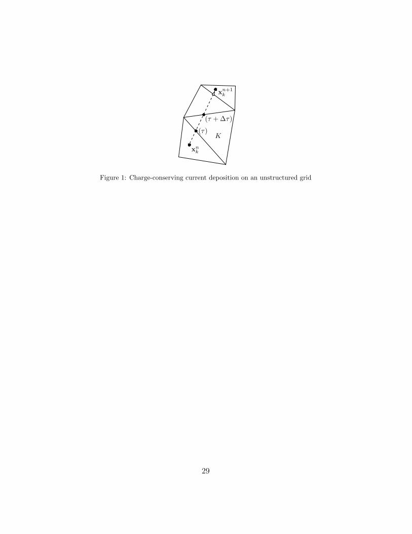
functions ϕi of Np−1(Th; Ω). A sketch of the particle trajectory is Figure 1.In the case of point particles (S = δ) their value is

Jn+ 1

2i := 〈Jn+ 1

2h ,ϕi〉 = 〈Jn+ 1

2S ,ϕi〉 =

N∑k=1

qwk

∫ tn+1

tn

v(pk(t))ϕi(xk(t))dt

∆t

(22)

and for piecewise affine trajectories the function t 7→ vn+ 1

2k ·ϕi(xk(t)) is itself

polynomial on every time interval [τ, τ + ∆τ ] ⊂ [tn, tn+1] that a particlespends inside a cell. In particular a Gauss formula with enough quadraturepoints is exact, i.e.∫ τ+∆τ

τ

ϕi(xk(t))dt

∆t=

∆τ

2∆t

q∑j=1

λj ϕi

(xk(τj)

)where q needs to be chosen in compliance with the degree of the FiniteElement functional space (for instance, with the above choice of Nedelecelements one must take q ≥ p+1

2if a Gauss-Legendre quadrature is used).

Remark 1. The case of Finite Difference schemes can be described withthe same arguments, since at lowest order (p = 1) the above Finite Element

11

method applied on a cartesian mesh with the mass lumping procedure of Cohenand Monk [16] is equivalent to the Yee scheme [32]. The above depositionmethod then coincides with that of Villasenor and Buneman [42].

4.2. Where enforcing a naive discrete continuity equations is not enough

If the above procedure gives satisfactory results when applied to FiniteDifference and curl-conforming Finite Element schemes, it is no longer thecase when applied to more general solvers such as the Discontinuous Galerkinmethod [15, 25].

To understand the reasons of this failure and propose a more robustpath for designing charge conserving schemes, we may consider as a typicalexample the DG method with centered fluxes studied in, e.g., [24, 26]. There,the electric and magnetic fields are sought in fully discontinuous spaces suchas (16) (thus, in Pp−1(Th)2 and Pp−1(Th) respectively), as the solutions to

〈∂tEh,ϕ〉 − 〈Bh, curlhϕ〉+∑e∈Eh

〈Bh, [ϕ]〉e = − 1

ε0

〈Jh,ϕ〉

〈∂tBh, ϕ〉+ 〈Eh, curlhϕ〉 −∑e∈Eh,I

〈Eh, [ϕ]〉e = 0(23)

for all test functions ϕ and ϕ in Pp−1(Th)2 and Pp−1(Th). Here the operators

curlhu :=∑T∈Th

curlu|T and curlhu :=∑T∈Th

curlu|T

correspond to “broken curls” in the discontinuous spaces, and standard nota-tions are used for tangential jumps and averages: on interior edges (e ∈ Eh,I)shared by two cells T±e with outward normal unit vectors n±e we let

[u]e := (n−e × u|T−e

+ n+e × u|T+

e)|e and ue :=

1

2(u|T−

e+ u|T+

e))|e

and on boundary edges (e ∈ Eh \ Eh,I) shared by a single cell Te we denote

[u]e := (ne × u|Te)|e and ue := (u|Te)|e.

For scalar-valued functions u the definitions are formally the same, keepingin mind that n× u now corresponds to the vector (nyu,−nxu)T.

12

It is then easily verified that this (semi-discrete) system preserves a dis-crete Gauss law similar to that of the curl-conforming FEM (17). To do sowe define

curldgh : Pp−1(Th)2 → Pp−1(Th) and curldg

h : Pp−1(Th)→ Pp−1(Th)2 (24)

by the relations

〈curldgh u, ϕ〉 = 〈u, curlhϕ〉 −

∑e∈Eh,I

〈u, [ϕ]〉e, ϕ ∈ Pp−1(Th) (25)

and

〈curldgh u,ϕ〉 = 〈u, curlhϕ〉 −

∑e∈Eh

〈u, [ϕ]〉e, ϕ ∈ Pp−1(Th)2, (26)

so that (23) corresponds to the abstract system (10) with discrete curls givenby (24)-(26). Here a standard computation involving Green formulas yields

curldgh = (curldg

h )∗ (27)

so that the associated evolution operator is skew-symmetric because of thedifferent signs in Ampere and Faraday’s laws. Setting then

graddgh : Lp(Th; Ω) 3 u 7→ gradu ∈ Pp−1(Th)2 (28)

(which is legitimate since gradLp(Th; Ω) ⊂ Pp−1(Th)2) and

divdgh := (−graddg

h )∗ : Pp−1(Th)2 → Lp(Th; Ω), (29)

we observe that the “structure” relation (12) holds also true in this DGcontext: for u ∈ Pp−1(Th) we have indeed divdg

h curldgh u ∈ Lp(Th; Ω) and

〈divdgh curldg

h u, ϕ〉 = −〈curldgh u,gradϕ〉 = −〈u, curldg

h gradϕ〉 = 0

for all ϕ ∈ Lp(Th; Ω), by using (27) and the fact that curldgh coincides with

the regular curl on the curl-conforming finite element field gradϕ.In particular, arguing as in Section 4.1 we find that by discretizing the

current density as in (22) we preserve the Gauss law divdgh Eh = ρh/ε0, i.e.,

〈Eh,−gradϕ〉 = 〈 1

ε0

ρh, ϕ〉 ϕ ∈ Lp(Th; Ω). (30)

13

While this could seem at first glance a quite natural discretization of thecontinuous Gauss law, one intuitively feels that by taking test functions inthe same space as in the conforming case (20) with Eh now belonging toa presumably larger discontinuous space will result in a discrete Gauss law(30) that is too weak. And indeed, the corresponding scheme is known to beunstable over large simulations times, as small errors accumulate into largedeviations, see e.g. [40] and the numerical results presented in Section 5.

4.3. Enforcing a “strong enough” discrete continuity equation

To answer the question raised in the previous Section – namely: is a givendiscrete Gauss law strong enough to ensure long-time stability? – we mayobserve that in the skew-symmetric case (14) where Im curlh = (ker curlh)

⊥,the “structure” relation (12) identified above can be restated as

(ker curlh)⊥ ⊂ ker divh . (31)

However, while this embedding is needed to guarantee that a Gauss lawinvolving the discrete operator divh will be preserved by the scheme, it doesnot say anything on the strength of this law. Specifically, the latter shouldallow to characterize the discrete longitudinal part of the electric fields, i.e.,the fields in ker curlh, since their temporal growth is not controlled in theevolution equation (10). Thus, we see that in order for the discrete Gausslaw to be strong enough to ensure long-time stability, the discrete divergenceoperator should satisfy

ker curlh ⊂ (ker divh)⊥

as it is the case for the continuous operators. Since this embedding is justthe opposite to (31), in the program (10)-(12) the proper “structure” relationshould be

(ker curlh)⊥ = ker divh (32)

and it is not difficult to verify that numerical schemes satifsying these prop-erties are stable over large simulation times.

Note that when applied to the curl-conforming method (17) the aboverelation amounts to

ker curlh = Im gradh

which simply expresses the fact that Lp(Th; Ω)grad−→ Np−1(Th; Ω)

curl−→ P(Th)is an exact sequence, a property known for long as essential to the spectral

14

correctness of the scheme [8, 14, 17, 38, 1]. However (32) does not hold forthe discrete operators defined by (25) and (29) in the DG case.

To design charge-conserving current deposition schemes that are consis-tent with general solvers we are thus left with the following tasks:

i) characterize the kernel of the discrete curl operator defined by theMaxwell solver (10);

ii) find a discrete divergence operator that satisfies the structure relation(32);

iii) define the discrete current Jh seen by the Maxwell solver in such away that a discrete continuity equation (11) based on this consistentdivergence is satisfied.

However recent this approach has already proven successful [12, 34], andwhen applied to the above DG solver it leads to depositing the current witha “corrected” Galerkin projection, see Section 4.5 below.

4.4. A shortcut: discretizing the sources and the curl in a compatible way

In the case of a pure Maxwell problem where the exact current densityJ is known, the above analysis still applies but a conceptually shorter pathto long-time stability is available. In [13] it was indeed realised that it waspossible to characterize approximation operators J 7→ Jh that provide long-time stability properties to the scheme (10), without any explicit reference toeither a discrete continuity equation or a discrete Gauss law (despite the factthat the motivation for such a characterization is driven by a compatibilityissue with the Gauss law).

Again, the starting point is to consider the spectral structure of the evo-lution operator involved in the Maxwell system. At the continuous level first,this is conveniently done in the skew-symmetric (perfect conductor bound-aries) and source-free case by rewriting the Ampere and Faraday equationsin a compact form

∂U

∂t−AU = 0 with U =

(EcB

), A = c

(0 curl

−(curl)∗ 0

)and the associated Gauss laws as

DU = 0 with D =

((grad)∗ 0

0 div

).

15

Using the skew-symmetry of A we can see that ImA = (kerA)⊥ ⊂ kerD,which expresses the fact that the Gauss law is preserved (DA = 0). Butagain, more important is the stronger property

(kerA)⊥ = kerD.

Indeed, using again the skew-symmetry of A we may decompose

L2 = kerA ⊕ (kerA)⊥ with

kerA = U : ∂U

∂t= 0

(kerA)⊥ = Span(U : ∂U∂t

= iωU : ω 6= 0)

so that the Gauss laws actually mean that the admissible solutions are thosewhich contain no stationary mode. We may now want to reproduce thisgeometric property at the discrete level. Considering a scheme

∂Uh∂t−AhUh = 0

where the approximation Ah of A satisfies Ah = −A∗h as in the FEM andDG examples shown above, we may state that in the absence of sources, Uhsatisfies a “fundamental” discrete Gauss law if it contains no stationary modewith respect to Ah, namely

Uh ∈ (kerAh)⊥.

Now, using the skew-symmetry of Ah one readily sees that this is in factequivalent with a property of the initial data, U0

h ∈ (kerAh)⊥. Turning tothe case with a source term

∂U

∂t−AU = F :=

(− 1ε0J

0

),

a less obvious step is to find a characterization for the solutions of

∂Uh∂t−AhUh = Fh := ΠhF (33)

that is compatible with the above interpretation of the divergence constraints.A minimal requirement is to ask that in the case where the exact solution con-tains no (continuous) stationary mode, its approximate counterpart shouldcontain no (discrete) stationary mode as well. Thus, we may ask that

U ∈ (kerA)⊥ =⇒ Uh ∈ (kerAh)⊥

16

and using once again the skew-symmetry of A and Ah this can be expressedequivalently on the data, as

U0, F ∈ (kerA)⊥ =⇒ U0h ,ΠhF ∈ (kerAh)⊥.

Now, since (kerA)⊥ = ImA and (kerAh)⊥ = ImAh, the latter condition es-sentially means that for any continuous field W , there should exist a discreteWh ≈ W such that ΠhAW = AhWh. This leads to call Gauss-compatible(on a given space V in the domain of A) a scheme of the form (33) for whichthere exists an approximation operator Πh such that

ΠhA = AhΠh holds on V . (34)

Quite surprisingly, this minimal characterization suffices to provide long timestability. Indeed in [13] it is shown that Gauss-compatible schemes satisfythe error estimate

‖(Uh − ΠhU)(t)‖ ≤ ‖U0h − ΠhU

0‖+

∫ t

0

‖(Πh − Πh)∂tU(s)‖ ds, t ≥ 0,

which implies that Uh cannot deviate from the stationary solutions to (33).And, as was the case for the structure preserving properties identified inSection 4.3, it can be shown that the compatibility condition (34) is satisfiedfor the curl-conforming finite element methods discussed above and in theDiscontinuous Galerkin case suitable projectors can be defined, see [13, 10,34].

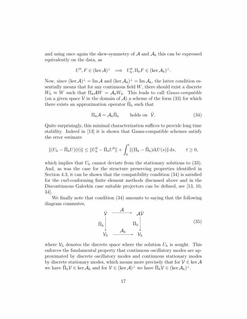
We finally note that condition (34) amounts to saying that the followingdiagram commutes,

V AV

Vh Vh

Πh

A

Πh

Ah

(35)

where Vh denotes the discrete space where the solution Uh is sought. Thisenforces the fundamental property that continuous oscillatory modes are ap-proximated by discrete oscillatory modes and continuous stationary modesby discrete stationary modes, which means more precisely that for V ∈ kerAwe have ΠhV ∈ kerAh and for V ∈ (kerA)⊥ we have ΠhV ∈ (kerAh)⊥.

17

4.5. Application to DG and DG-PIC schemes: current correctionWhen applied to a centered DG discretization of the 2d Maxwell system

as described in Section 4.2, both the above strategies (be it the “charge-conserving” one described in Section 4.3 or the “Gauss-compatible” one de-scribed in Section 4.4) lead to defining the DG current density Jh ∈ Pp−1(Th)2

as a corrected projection of the exact current, of the form

〈Jh,ϕi〉 := 〈J ,Phϕi〉 for ϕi ∈ Pp−1(Th)2. (36)

Here Ph denotes a finite element interpolation on the Nedelec space (15)that is extended to DG fields by local averaging of the edge-based degrees offreedom. For a detailed description we refer to [12, 34] for the cartesian case.

In practice, it is possible to implement this corrected projection in twosteps as follows.

• first, perform a standard Galerkin (i.e., orthogonal) projection of thecurrent on some (e.g., DG) space Vh ⊃ Np−1(Th; Ω) by computing theproducts

J j := 〈J , ϕj〉 for ϕj ∈ Vh ; (37)

• then post-process the resulting values to compute the products of thecompatible current Jh defined in (36) with

J i := 〈Jh,ϕi〉 =∑j

ci,jJ j for ϕi ∈ Pp−1(Th)2 (38)

where the coefficients ci,j are such that Phϕi =∑

j ci,jϕj. This is al-

ways possible given that Vh contains the curl-conforming Nedelec space.Moreover it should be emphasized that (38) corresponds to applying asparse (band) matrix to the array J , since the projection Ph is local.

For a DG-PIC scheme the same approach can be used to deposit thecurrent from the particles, and the above steps are then to be applied toJ = JS. Note that in a fully discrete setting the latter should be definedusing time-averages, as described in Section 4.1.

Remark 2. In order to justify that (36) is indeed a Gauss-compatible ap-proximation for the current, one uses the fact that for a well-designed pro-jection operator Ph, the centered DG curl operator defined in (25) satisfies

curldgh = curlPh : Pp−1(Th)2 → Pp−1(Th).

see [12, 34]. In the 3d-case things are slightly different, as an additionalprojection must be added after the curl, see [13].

18

5. Numerical illustrations

5.1. Maxwell’s equations with analytical source (Depeyre-Issautier test case)

As a first test case we consider the Maxwell equations with an analyticalcurrent source that has been proposed to study the numerical charge conser-vation properties in [27, 20] and also considered in [40] to assess the stabilityof 3d DG solvers with hyperbolic field correction.

Here the problem is posed in a metallic cavity Ω = [0, 1]2, with articifialpermittivity ε0 and light speed c equal to one. The given current source is

J(t, x, y) = (cos(t)− 1)

(π cos(πx) + π2x sin(πy)π cos(πy) + π2y sin(πx)

)− cos(t)

(x sin(πy)y sin(πx)

)and an exact solution for this source is

E(t, x, y) = sin(t)

(x sin(πy)y sin(πx)

)and

B(t, x, y) = (cos(t)− 1)(πy cos(πx)− πx cos(πy)

).

Note that for this solution the associated charge density reads

ρ(t, x, y) = sin(t)(

sin(πx) + sin(πy)).

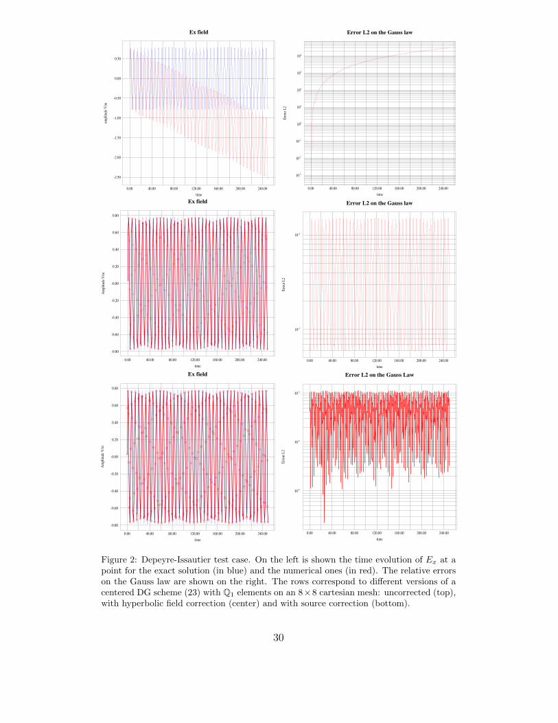
In Figure 2 we show different results obtained with a centered DG schemeof the form (23) using piecewise Q1 elements on a 8× 8 cartesian mesh andseveral correction methods. To assess the charge conservation propertiesof the resulting schemes we plot the time evolution of Ex and the erroron the Gauss law divE − ρ (computed inside every cell where the field islocallyH(div)). Here we compare the results given by the basic non-correctedscheme where Jh is defined as the standard orthogonal projection of J onthe DG space (top row) with those obtained either with a hyperbolic fieldcorrection scheme (center row), or with a source correction computed withthe technique described in Section 4.5 (bottom row). The advantage of usinga correction methods is blatant. Time-wise, we note that while the sourcecorrection scheme consumes about the same amount of resources than thebasic one, the field correction method requires a significant increase of 33%in cpu time.

19

5.2. Electromagnetic PIC test cases

5.2.1. The beam test case

In order to test the behaviour of Maxwell solvers coupled with particleswe next show simulations of a beam test case which is known to strongly relyon the Gauss law being well satisfied, see for instance [3, 40]. In this testcase the domain Ω := [0, 1]2 \ (B+ ∪ B−) consists of a square of 1 m widthminus two disks of radius 0.2 m with respective centers at (1, 1) and (1, 0), seeFigure 3. A bunch of electrons is emitted with current density 500 Am−2 onthe left boundary (a metallic cathode) and accelerated by a strong externalfield Eext = −gradφext created by the fixed potential maintained betweenthe cathode (where φ = 0 V) and on the anode (the two metallic arcs whereφ = 105 V). The right, top and bottom boundaries are absorbing. After afirst transient phase the beam propagates towards the right boundary witha steady-state self-consistent field, as depicted in Figure 3.

In Figure 4 we then display the Ex field obtained with three differentschemes: in the left panel we show the field computed by the curl-conformingscheme (17) with edge-elements of maximal degree p = 2, coupled withthe conservative current deposition scheme described in Section 4.1. In thecenter and right panels we then plot the fields obtained with the centeredDG scheme (23) using discontinous elements of degree p = 1. Here thecenter panel corresponds to the uncorrected case where the current density isdeposited with a standard method as in Equation (37) alone, which is neitherGauss-compatible nor charge-conserving in the sense specified in Sections 4.3and 4.4. Finally the right panel shows the field computed with a Gauss-compatible current deposition corresponding to the combined steps (37) and(38). The effectiveness of the latter method is obvious, and is also supportedby longer simulations.

5.2.2. 2D matter-photons interaction inside a metallic cavity

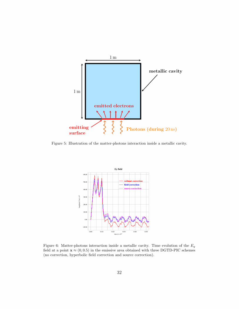
We next consider a metallic cavity Ω = [−0.5, 0.5]× [0.5, 0.5] whose lowerside is hit by a flux of photons during 20 [ns] as depicted in Figure 5. Herethe energy of the photons is such that electrons are extracted from the wall,and we simulate the electrons within the cavity. During the emissive phasewe inject 200 numerical particles per time step, using an emitting surface ofwidth 600 [mm] and a current density of 1800 Am−2. The initial velocity ofthe electrons is normal to the wall and corresponds to a kinetic energy of10 keV.

20

Before describing the numerical results, we emphasize that there is aproperty that any qualitatively correct simulation should satisfy. Indeed,since all the emitted electrons are bound to eventually hit and be absorbedby a boundary of the metallic cavity, we observe that all the positive chargescreated on the cavity surface by the initial loss of these electrons will beeventually neutralized. It follows that there should be no static field at theend of the correct simulations.

In Figures 6 and 7 we compare the results obtained with a centered DGscheme of the form (23) using piecewise Q1 elements on a 60× 60 cartesianmesh and several correction methods, namely the uncorrected scheme (stan-dard projection of the current density carried by the particles), a scheme withhyperbolic field correction and a scheme with source correction as describedin Section 4.5.

Here to assess the quality of the simulations we first plot in Figure 6 theEy field at a point x ≈ (0, 0.5) in the emissive area, for the three versions ofthe scheme. During the emission time the three curves are almost identical,but after the electrons are emitted the curve corresponding to the uncorrectedscheme (in red) does not oscillate around zero, which indicates a physicallyincorrect behavior as was noticed above. We interpret this phenomenon asbeing typical of a bad preservation of the Gauss law. Indeed at the continuouslevel the solutions are only composed of genuinely oscillating fields, at leastwhen all the electrons have been absorbed back by the metallic walls of thecavity. On the other hand, we observe that both correction methods producethe expected behavior, i.e., an field oscillating around zero.

The same phenomenon is visible in Figure 7 where the Ey field is shownin the entire domain together with the numerical particles at 5 ns, 10 nsand 50 ns. The latter snapshot corresponds to a time where the all theelectrons have left the domain, however a strong residual field can be seenclose to the emitting area. In the corrected DGTD-PIC schemes this residualfield is absent which shows the effectiveness of both correction techniques tonumerically preserve the charge, be it the hyperbolic field correction or thesource correction method.

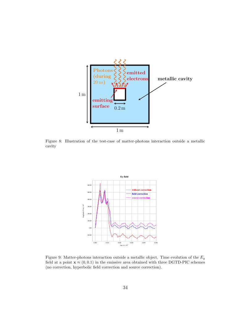
5.2.3. 2D matter-photons interaction outside a metallic object

In this test case we consider a metallic object whose upper side is hitby a flux of photons during 20 ns, in such a way that the electrons are nowextracted out of the object and propagate away from it, as depicted Figure 8.The emitting object is now a square of 0.2 m width, and for computational

21

purposes it is enclosed inside a larger metallic square of 1 m width. Again,the emissive phase is modelled by injecting 200 numerical particles per timestep corresponding to a current density of 1800 Am−2, and the initial velocityof the electrons is normal to the wall and corresponds to a kinetic energy of10 keV.

Unlike in the previous test case where all the emitted electrons wouldeventually be absorbed back by a metallic surface in contact with the emis-sive area, a significant fraction of the charge is now expected to leave the sim-ulation domain (or be absorbed by the surrounding metallic surface) withoutcoming back. In particular, a net positive charge should remain on the sur-face of the emitting metallic object and a non-zero static field is expected tobe observed around it.

As above, Figures 9 and 10 allow to compare the results obtained withdifferent versions of a centered DGTD-PIC scheme of the form (23) usingpiecewise Q1 elements on a 60× 60 cartesian mesh: the uncorrected scheme,the scheme with hyperbolic field correction and the scheme with the sourcecorrection described in Section 4.5.

In Figure 9 we show the Ey field at a point x ≈ (0, 0.1) in the emis-sive area, for the three versions of the scheme. Again, the values are almostidentical during the emission time, but after the electrons are emitted thebehavior of the three curves is very different. First, we see that the curve cor-responding to the uncorrected scheme oscillates around a nonzero value whichdoes not match the expected value (determined with a reference FDTD-PICcode). Moreover this value is not stable, as longer simulations show thatit decreases with time: this reflects the bad conservation of charge in theuncorrected scheme. Turning to the hyperbolic correction curve, we observethat it eventually oscillates around zero. As was explained above, this is notqualitatively correct and can be interpreted as a numerical evidence of a badpreservation of the Gauss law. Finally, the curve produced by the sourcecorrection method has the expected behavior. Indeed, after 20 ns it oscil-lates around a constant value of 7.5 V/m which is confirmed by a referenceFDTD-PIC scheme.

These findings are confirmed in Figure 10 where the Ey field is shown inthe entire domain together with the numerical particles at 5 ns, 10 ns and50 ns.

Again, notable differences are visible in the latter snapshot which corre-sponds to a time where the electrons have left the computational domain: inthe uncorrected scheme (top row) a strong unphysical field is present close to

22

the emissive area, in the field corrected scheme (center row) the residual fieldis close to zero which does not match with the presence of positive charges onthe inner metallic object, and finally the source correction scheme (bottomrow) computes a qualitatively correct field.

We note that the reason why the field correction method does not givecharge-conserving results for this test case lies in the fact that the boundaryconditions are not properly taken into account in the propagation of thecorrected field. To do so it would be necessary to represent the surfacecharge density on the emitting object, which requires additional steps in thediscretization process that are not straighfoward. In particular, this test-casereflects the advantage of the source correction method for DGTD-PIC codes,as it overcomes the need of properly representing the surface charge density.

6. Conclusion

In the numerical approximation of Maxwell’s equations an adequate dis-cretization of the divergence constraints (or involutions) plays a major rolein getting accurate and stable solutions over long simulation times. Thisproblem becomes even more important in the presence of sources. Becausethese constraints put additional requirements on the discrete solutions thereare essentially too options: either relax them by adding additional degreesof freedom, or make them compatible with the discretization. The formerchoice corresponds to field correction methods and we have described thelatter as source correction methods. In this paper we set the framework forboth techniques, reviewed different implementations and also provided somenumerical illustrations highlighting the problem and its solutions.

Acknowledgement:. This work was performed in part during Marie Mounier’sPhD thesis in the Nucletudes company, which was supported by DGA .

[1] D.N. Arnold, R.S. Falk, and R. Winther. Finite element exterior cal-culus, homological techniques, and applications. Acta Numerica, pages1–55, 2006.

[2] R. Barthelme, P. Ciarlet Jr, and E. Sonnendrucker. Generalized formula-tions of Maxwell’s equations for numerical Vlasov–Maxwell simulations.Mathematical Models and Methods in Applied Sciences, 17(05):657–680,2007.

23

[3] R. Barthelme and C. Parzani. Numerical charge conservation in particle-in-cell codes. Numerical Methods for Hyperbolic and Kinetic Problems,pages 7–28, 2005.

[4] D. Boffi. Compatible Discretizations for Eigenvalue Problems. In Com-patible Spatial Discretizations, pages 121–142. Springer New York, NewYork, NY, 2006.

[5] D. Boffi. Finite element approximation of eigenvalue problems. ActaNumerica, 19:1–120, 2010.

[6] D. Boffi, F. Brezzi, and M. Fortin. Mixed finite element methods and ap-plications, volume 44 of Springer Series in Computational Mathematics.Springer, 2013.

[7] J.P. Boris. Relativistic plasma simulations - optimization of a hybridcode. In Proc. 4th Conf. Num. Sim. of Plasmas, (NRL Washington,Washington DC), pages 3–67, 1970.

[8] A. Bossavit. Solving Maxwell equations in a closed cavity, and the ques-tion of ’spurious modes’. IEEE Transactions on Magnetics, 26(2):702–705, March 1990.

[9] A. Buffa and I. Perugia. Discontinuous Galerkin Approximation ofthe Maxwell Eigenproblem. SIAM Journal on Numerical Analysis,44(5):2198–2226, January 2006.

[10] M. Campos Pinto. Constructing exact sequences on non-conformingspaces. Submitted, 2015.

[11] M. Campos Pinto, S. Jund, S. Salmon, and E. Sonnendrucker. Chargeconserving fem-pic schemes on general grids. C.R. Mecanique, 342(10-11):570–582, 2014.

[12] M. Campos Pinto and M. Mounier. Charge-conserving DG-PIC schemeson 2d cartesian meshes. In preparation.

[13] M. Campos Pinto and E. Sonnendrucker. Gauss-compatible Galerkinschemes for time-dependent Maxwell equations. http://hal.upmc.fr/hal-00969326, 2014.

24

[14] S. Caorsi, P. Fernandes, and M. Raffetto. On the convergence of Galerkinfinite element approximations of electromagnetic eigenproblems. SIAMJournal on Numerical Analysis, 38(2):580–607 (electronic), 2000.

[15] B Bernardo Cockburn, George Karniadakis, and Chi-Wang Shu. Dis-continuous Galerkin methods : theory, computation, and applications.Berlin ; New York : Springer, 2000.

[16] G. Cohen and P. Monk. Gauss point mass lumping schemes forMaxwell’s equations. Numerical Methods for Partial Differential Equa-tions, 14(1):63–88, 1998.

[17] M. Costabel and M. Dauge. Computation of resonance frequencies forMaxwell equations in non-smooth domains. In Topics in computationalwave propagation, pages 125–161. Springer, Berlin, 2003.

[18] N. Crouseilles, P. Navaro, and E. Sonnendrucker. Charge conservinggrid based methods for the Vlasov-Maxwell equations. C. R. Mecanique,342(10-11):636–646, 2014.

[19] A. Dedner, F. Kemm, D. Kroner, C.-D. Munz, T. Schnitzer, and We-senberg M. Hyperbolic divergence cleaning for the MHD equations. J.Comput. Phys., 175:645–673, 2002.

[20] S. Depeyre and D. Issautier. A new constrained formulation ofthe Maxwell system. Rairo-Mathematical Modelling and NumericalAnalysis-Modelisation Mathematique Et Analyse Numerique, 31(3):327–357, 1997.

[21] J.W. Eastwood. The virtual particle electromagnetic particle-meshmethod. Computer Physics Communications, 64(2):252–266, 1991.

[22] J.W. Eastwood, W. Arter, NJ Brealey, and RW Hockney. Body-fittedelectromagnetic PIC software for use on parallel computers. ComputerPhysics Communications, 87(1):155–178, 1995.

[23] T.Zh. Esirkepov. Exact charge conservation scheme for particle-in-cellsimulation with an arbitrary form-factor. Computer Physics Communi-cations, 135(2):144–153, 2001.

25

[24] L. Fezoui, S. Lanteri, S. Lohrengel, and S. Piperno. Convergence andstability of a discontinuous Galerkin time-domain method for the 3D het-erogeneous Maxwell equations on unstructured meshes. ESAIM: Mathe-matical Modelling and Numerical Analysis, 39(6):1149–1176, November2005.

[25] J.S. Hesthaven and T. Warburton. Nodal High-Order Methods on Un-structured Grids. Journal of Computational Physics, 181(1):186–221,September 2002.

[26] J.S. Hesthaven and T. Warburton. High-order nodal discontinuousGalerkin methods for the Maxwell eigenvalue problem. PhilosophicalTransactions of the Royal Society A: Mathematical, Physical and Engi-neering Sciences, 362(1816):493–524, March 2004.

[27] Didier Issautier, Frederic Poupaud, Jean-Pierre Cioni, and Loula Fe-zoui. A 2-D Vlasov-Maxwell solver on unstructured meshes. In Thirdinternational conference on mathematical and numerical aspects of wavepropagation, pages 355–371, 1995.

[28] A.B. Langdon. On enforcing Gauss’ law in electromagnetic particle-in-cell codes. Comput. Phys. Comm., 70:447–450, 1992.

[29] R. Leis. Initial boundary value problems in mathematical physics. JohnWiley & Sons Ltd, 1986.

[30] P.J. Mardahl and J.P. Verboncoeur. Charge conservation in electromag-netic pic codes; spectral comparison of boris/dadi and langdon-mardermethods. Computer physics communications, 106(3):219–229, 1997.

[31] B. Marder. A method for incorporating Gauss’s law into electromagneticPIC codes. J. Comput. Phys., 68:48–55, 1987.

[32] P. Monk. An analysis of Nedelec’s method for the spatial discretizationof Maxwell’s equations. Journal of Computational and Applied Mathe-matics, 47(1):101–121, 1993.

[33] Haksu Moon, Fernando L Teixeira, and Yuri A Omelchenko. Exactcharge-conserving scatter–gather algorithm for particle-in-cell simula-tions on unstructured grids: A geometric perspective. Computer PhysicsCommunications, 194:43–53, 2015.

26

[34] Marie Mounier. Resolution des equations de Maxwell-Vlasov sur mail-lage cartesien non conforme 2D par un solveur Galerkin Discontinu.PhD thesis, IRMA, universite de Strasbourg, 2014. https://tel.

archives-ouvertes.fr/tel-01081560/.

[35] C.-D. Munz, P. Omnes, R. Schneider, E. Sonnendrucker, and U. Voß.Divergence Correction Techniques for Maxwell Solvers Based on a Hy-perbolic Model. Journal of Computational Physics, 161(2):484–511, July2000.

[36] C.-D. Munz, R. Schneider, E. Sonnendrucker, and U. Voß. Maxwell’sequations when the charge conservation is not satisfied. Comptes Rendusde l’Academie des Sciences-Series I-Mathematics, 328(5):431–436, 1999.

[37] J.-C. Nedelec. Mixed finite elements in R3. Numerische Mathematik,35(3):315–341, 1980.

[38] R.N. Rieben, G.H. Rodrigue, and D.A. White. A high order mixedvector finite element method for solving the time dependent Maxwellequations on unstructured grids. Journal of Computational Physics,204(2):490–519, April 2005.

[39] N.J. Sircombe and T.D. Arber. Valis: A split-conservative scheme forthe relativistic 2d vlasov-maxwell system. J. Comput. Phys., 228:4773–4788, 2009.

[40] A. Stock, J. Neudorfer, R. Schneider, C. Altmann, and C.-D. Munz.Investigation of the Purely Hyperbolic Maxwell System for DivergenceCleaning in Discontinuous Galerkin based Particle-In-Cell Methods. InCOUPLED PROBLEMS 2011 IV International Conference on Com-putational Methods for Coupled Problems in Science and Engineering,2011.

[41] T. Umeda, Y. Omura, T. Tominaga, and H. Matsumoto. A newcharge conservation method in electromagnetic particle-in-cell simula-tions. Computer Physics Communications, 156(1):73–85, 2003.

[42] J. Villasenor and O. Buneman. Rigorous charge conservation for lo-cal electromagnetic field solvers. Computer Physics Communications,69(2):306–316, 1992.

27

[43] K.S. Yee. Numerical solution of initial boundary value problems in-volving maxwell’s equations in isotropic media. IEEE Trans. AntennasPropag., 14(3):302–307, May 1966.

28

(τ)

xn+1k

xnk

K

(τ + ∆τ)

Figure 1: Charge-conserving current deposition on an unstructured grid

29

Ex field

-2.50

-2.00

-1.50

-1.00

-0.50

0.00

0.50

ampli

tude V

/m

0.00 40.00 80.00 120.00 160.00 200.00 240.00time

Error L2 on the Gauss law

10-3

10-2

10-1

100

101

102

103

104

Erreu

r L2

0.00 40.00 80.00 120.00 160.00 200.00 240.00time

Ex field

-0.80

-0.60

-0.40

-0.20

-0.00

0.20

0.40

0.60

0.80

Ampli

tude V

/m

0.00 40.00 80.00 120.00 160.00 200.00 240.00time

Error L2 on the Gauss law

10-3

10-2

Erreu

r L2

0.00 40.00 80.00 120.00 160.00 200.00 240.00time

Ex field

-0.80

-0.60

-0.40

-0.20

-0.00

0.20

0.40

0.60

0.80

Ampli

tude V

/m

0.00 40.00 80.00 120.00 160.00 200.00 240.00time

Error L2 on the Gauss Law

10-5

10-4

10-3

Erreu

r L2

0.00 40.00 80.00 120.00 160.00 200.00 240.00time

Figure 2: Depeyre-Issautier test case. On the left is shown the time evolution of Ex at apoint for the exact solution (in blue) and the numerical ones (in red). The relative errorson the Gauss law are shown on the right. The rows correspond to different versions of acentered DG scheme (23) with Q1 elements on an 8×8 cartesian mesh: uncorrected (top),with hyperbolic field correction (center) and with source correction (bottom).

30

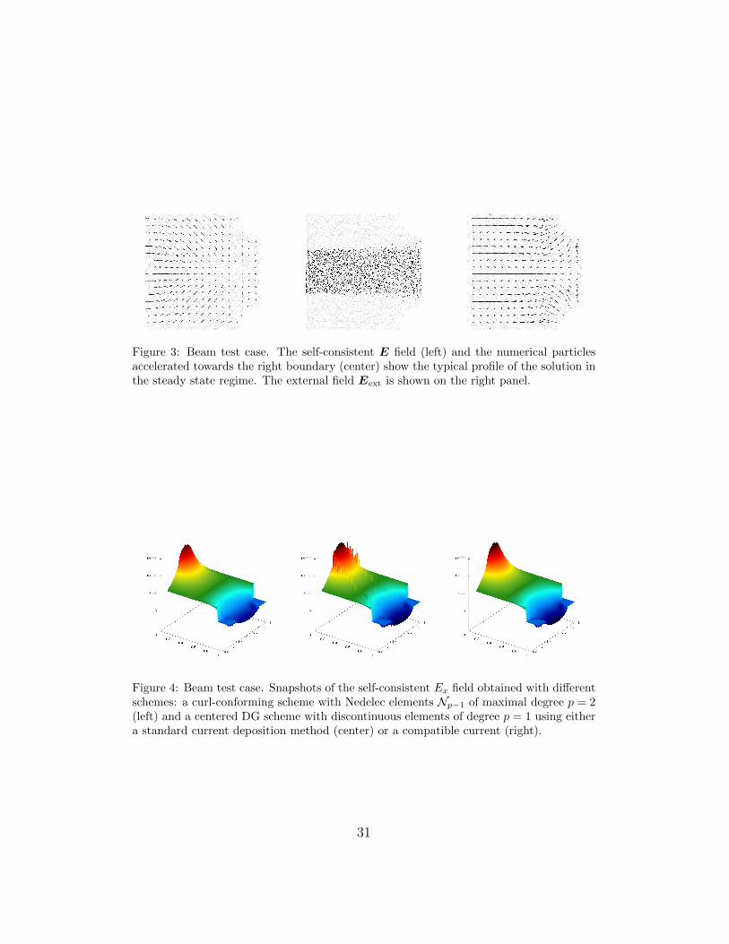
Figure 3: Beam test case. The self-consistent E field (left) and the numerical particlesaccelerated towards the right boundary (center) show the typical profile of the solution inthe steady state regime. The external field Eext is shown on the right panel.

Figure 4: Beam test case. Snapshots of the self-consistent Ex field obtained with differentschemes: a curl-conforming scheme with Nedelec elements Np−1 of maximal degree p = 2(left) and a centered DG scheme with discontinuous elements of degree p = 1 using eithera standard current deposition method (center) or a compatible current (right).

31

metallic cavity

1 m

1 m

emittingsurface

emitted electrons

Photons (during 20 ns)

Figure 5: Illustration of the matter-photons interaction inside a metallic cavity.

Ey field

-100.00

0.00

100.00

200.00

300.00

400.00

500.00

600.00

Ampli

tude (

V/m)

x 10

3

0.000 0.010 0.020 0.030 0.040 0.050time (s) x 10-6

without correctionfield correctionsource correction

Figure 6: Matter-photons interaction inside a metallic cavity. Time evolution of the Ey

field at a point x ≈ (0, 0.5) in the emissive area obtained with three DGTD-PIC schemes(no correction, hyperbolic field correction and source correction).

32

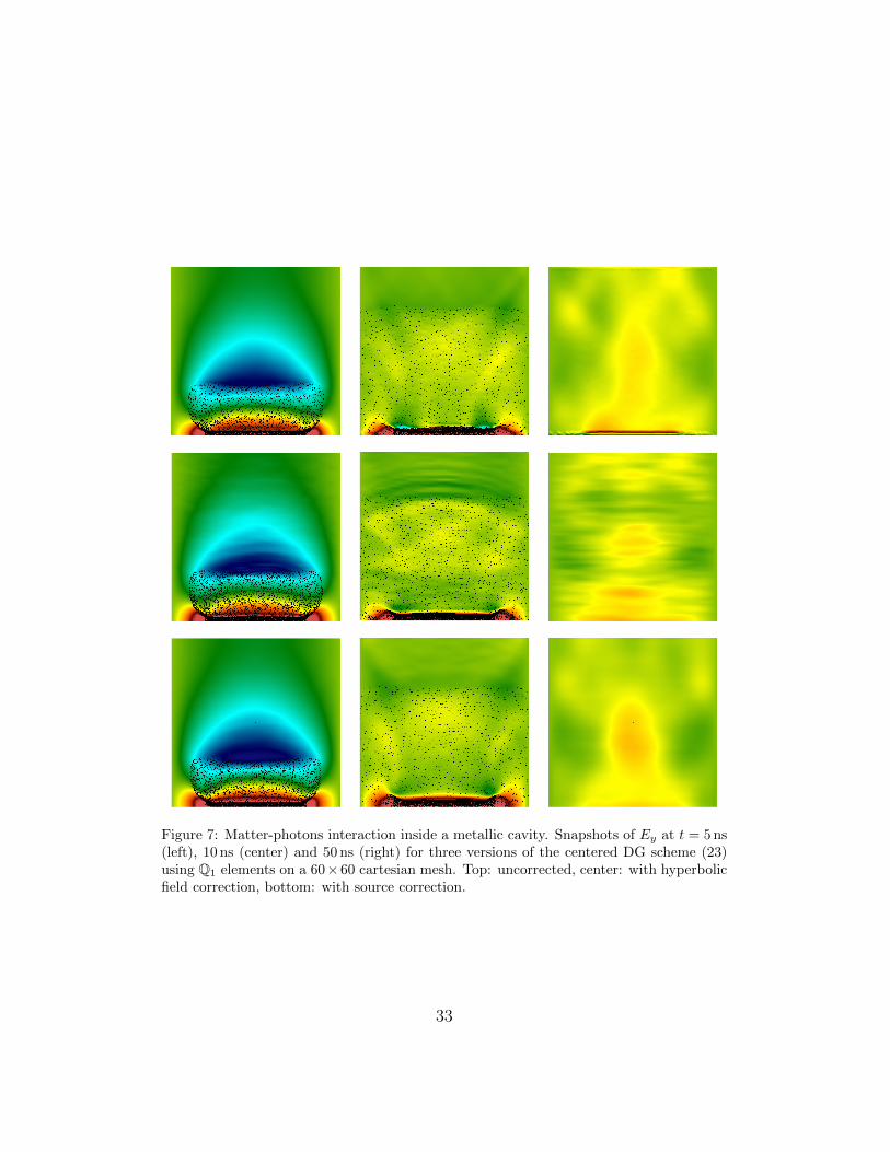
Figure 7: Matter-photons interaction inside a metallic cavity. Snapshots of Ey at t = 5 ns(left), 10 ns (center) and 50 ns (right) for three versions of the centered DG scheme (23)using Q1 elements on a 60×60 cartesian mesh. Top: uncorrected, center: with hyperbolicfield correction, bottom: with source correction.

33

metallic cavity

1 m

1 m

0.2 m

emittingsurface

emittedelectrons

Photons(during20 ns)

Figure 8: Illustration of the test-case of matter-photons interaction outside a metalliccavity

Ey field

-100.00

0.00

100.00

200.00

300.00

400.00

500.00

600.00

Ampli

tude (

V/m)

x 10

3

0.000 0.010 0.020 0.030 0.040 0.050time (s) x 10-6

without correctionfield correctionsource correction

Figure 9: Matter-photons interaction outside a metallic object. Time evolution of the Ey

field at a point x ≈ (0, 0.1) in the emissive area obtained with three DGTD-PIC schemes(no correction, hyperbolic field correction and source correction).

34

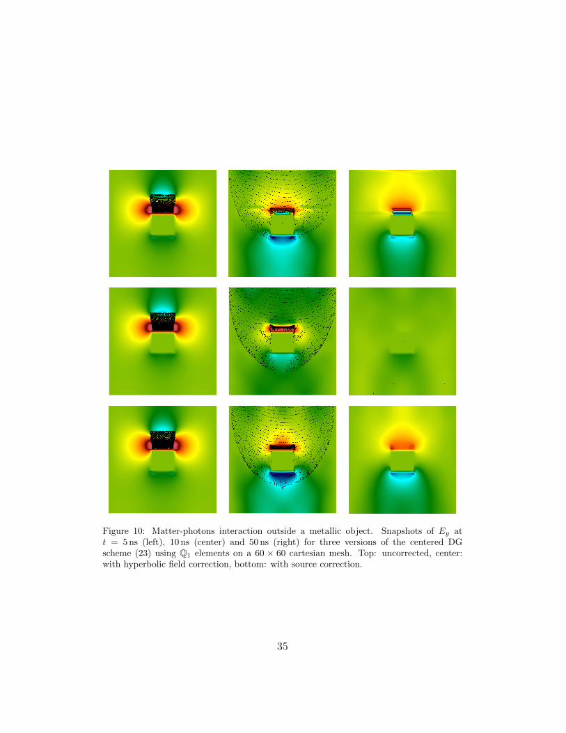
Figure 10: Matter-photons interaction outside a metallic object. Snapshots of Ey att = 5 ns (left), 10 ns (center) and 50 ns (right) for three versions of the centered DGscheme (23) using Q1 elements on a 60 × 60 cartesian mesh. Top: uncorrected, center:with hyperbolic field correction, bottom: with source correction.

35