handover strategies

3G TR 25.922 V2.0.0 (1999-12)Technical Report

3rd Generation Partnership Project;Technical Specification Group Radio Access Network;

Radio Resource Management Strategies(3G TR 25.922 version 2.0.0)

The present document has been developed within the 3rd Generation Partnership Project (3GPP TM) and may be further elaborated for the purposes of 3GPP.

The present document has not been subject to any approval process by the 3GPP Organisational Partners and shall not be implemented.This Specification is provided for future development work within 3GPP only. The Organisational Partners accept no liability for any use of this Specification.Specifications and reports for implementation of the 3GPP TM system should be obtained via the 3GPP Organisational Partners' Publications Offices.

3GPP

3G TR 25.922 V2.0.0 (1999-12)23G TR 25.922 version 2.0.0

Reference3TR/TSGR-0225922 U

Keywords<keyword[, keyword]>

3GPP

Postal address

3GPP support office address650 Route des Lucioles - Sophia Antipolis

Valbonne - FRANCETel.: +33 4 92 94 42 00 Fax: +33 4 93 65 47 16

Internethttp://www.3gpp.org

Copyright Notification

No part may be reproduced except as authorized by written permission.The copyright and the foregoing restriction extend to reproduction in all media.

© 1999, 3GPP Organizational Partners (ARIB, CWTS, ETSI, T1, TTA,TTC).All rights reserved.

3GPP

3G TR 25.922 V2.0.0 (1999-12)33G TR 25.922 version 2.0.0

Contents

Foreword ............................................................................................................................................................ 6

1 Scope........................................................................................................................................................ 7

2 References................................................................................................................................................ 7

3 Definitions and abbreviations .................................................................................................................. 73.1 Definitions ......................................................................................................................................................... 73.2 Abbreviations..................................................................................................................................................... 7

4 Idle Mode Tasks....................................................................................................................................... 94.1 Service type in Idle mode .................................................................................................................................. 94.2 Criteria for Cell Selection and Reselection........................................................................................................ 94.2.1 Cell Selection Criteria .................................................................................................................................. 94.2.2 Immediate Cell Evaluation........................................................................................................................... 94.2.3 Cell Re-selection ........................................................................................................................................ 104.3 Location Registration....................................................................................................................................... 10

5 RRC Connection Mobility ..................................................................................................................... 105.1 Handover ......................................................................................................................................................... 105.1.1 Strategy ...................................................................................................................................................... 105.1.2 Causes ........................................................................................................................................................ 105.1.3 Hard Handover ........................................................................................................................................... 115.1.4 Soft Handover ............................................................................................................................................ 115.1.4.1 Soft Handover Parameters and Definitions .......................................................................................... 115.1.4.2 Example of a Soft Handover Algorithm............................................................................................... 125.1.4.3 Soft Handover Execution...................................................................................................................... 135.1.5 Inter System Handover............................................................................................................................... 145.1.5.1 Handover 3G to 2G .............................................................................................................................. 145.1.6 Measurements for Handover ...................................................................................................................... 145.1.6.1 Monitoring of FDD cells on the same frequency.................................................................................. 145.1.6.2 Monitoring cells on different frequencies............................................................................................. 145.1.6.2.1 Monitoring of FDD cells on a different frequency.......................................................................... 145.1.6.2.2 Monitoring of TDD cells ................................................................................................................ 155.1.6.2.2.2 Setting of compressed mode parameters with prior timing information between FDD

serving cell and TDD target cells .............................................................................................. 155.1.6.2.3 Monitoring of GSM cells ................................................................................................................ 15

6 Admission Control ................................................................................................................................. 186.1 Introduction...................................................................................................................................................... 186.2 Examples of CAC strategies ............................................................................................................................ 186.3 Scenarios.......................................................................................................................................................... 196.3.1 CAC performed in SRNC .......................................................................................................................... 196.3.2 CAC performed in DRNC.......................................................................................................................... 196.3.2.1 Case of DCH......................................................................................................................................... 196.3.2.2 Case of Common Transport Channels .................................................................................................. 20

7 Radio Bearer Control ............................................................................................................................. 217.1 Usage of Radio Bearer Control procedures ..................................................................................................... 217.1.1 Examples of Radio Bearer Setup................................................................................................................ 217.1.2 Examples of Physical Channel Reconfiguration ........................................................................................ 217.1.2.1 Increased UL data, with switch from RACH/FACH to DCH/DCH ..................................................... 217.1.2.2 Increased DL data, no Transport channel type switching..................................................................... 227.1.2.3 Decrease DL data, no Transport channel type switching...................................................................... 227.1.2.4 Decreased UL data, with switch from DCH/DCH to RACH/FACH.................................................... 237.1.3 Examples of Transport Channel Reconfiguration ...................................................................................... 237.1.3.1 Increased UL data, with no transport channel type switching .............................................................. 237.1.3.2 Decreased DL data, with switch from DCH/DCH to RACH/FACH.................................................... 247.1.4 Examples of Radio Bearer Reconfiguration............................................................................................... 24

3GPP

3G TR 25.922 V2.0.0 (1999-12)43G TR 25.922 version 2.0.0

8 Dynamic Resource Allocation ............................................................................................................... 258.1 Code Allocation Strategies for FDD mode ...................................................................................................... 258.1.1 Introduction................................................................................................................................................ 258.1.2 Criteria for Code Allocation....................................................................................................................... 268.1.3 Example of code Allocation Strategies ...................................................................................................... 268.2 DCA (TDD)..................................................................................................................................................... 278.2.1 Channel Allocation..................................................................................................................................... 278.2.1.1 Resource allocation to cells (slow DCA).............................................................................................. 278.2.1.2 Resource allocation to bearer services (fast DCA) ............................................................................... 288.2.2 Measurements Reports from UE to the UTRAN........................................................................................ 28

9 Power Management ............................................................................................................................... 299.1 Variable Rate Packet Transmission ................................................................................................................. 299.1.1 Examples of Downlink Power Management.............................................................................................. 299.1.2 Examples of Uplink Power Management................................................................................................... 299.2 Site Selection Diversity Power Control (SSDT).............................................................................................. 299.3 Examples of balancing Downlink power ......................................................................................................... 309.3.1 Adjustment loop ......................................................................................................................................... 30

10 Radio Link Surveillance ........................................................................................................................ 3110.1 Mode Control strategies for tx diversity .......................................................................................................... 3110.1.1 TX diversity modes .................................................................................................................................... 3110.1.2 Mode Control Strategies............................................................................................................................. 3110.1.2.1 DPCH ................................................................................................................................................... 3110.1.2.2 Common channels ................................................................................................................................ 31

11 Codec mode control ............................................................................................................................... 3211.1 AMR mode control .......................................................................................................................................... 32

Appendix A: Simulations on Fast Dynamic Channel Allocation............................................................... 34A.1 Simulation environment................................................................................................................................... 34A.2 Results ............................................................................................................................................................. 34A.2.1 Macro UDD 144......................................................................................................................................... 34A.2.2 Micro UDD 384 ......................................................................................................................................... 35A.2.2.1 Code rate 1............................................................................................................................................ 35A.2.2.2 Code rate 2/3 ........................................................................................................................................ 36A.3 Conclusions...................................................................................................................................................... 36

Appendix B: Radio Bearer Control – Overview of Procedures: message exchange and parametersused ........................................................................................................................................ 37

B.1 Examples of Radio Bearer Setup ..................................................................................................................... 37B.1.1 RRC Parameters in RB Setup..................................................................................................................... 37B.1.2 RRC Parameters in RB Setup Complete .................................................................................................... 37B.2 Examples of Physical Channel Reconfiguration.............................................................................................. 37B.2.1 Increased UL data, with switch from RACH/FACH to DCH/DCH........................................................... 38B.2.1.1 RRC Parameters in Measurement Report............................................................................................. 38B.2.1.2 RRC Parameters in Physical Channel Reconfiguration........................................................................ 38B2.1.3 RRC Parameters in Physical Channel Reconfiguration Complete ....................................................... 38B.2.2 Increased DL data, no Transport channel type switching........................................................................... 38B.2.2.1 RRC Parameters in Physical Channel Reconfiguration........................................................................ 39B.2.2.2. RRC Parameters in Physical Channel Reconfiguration Complete ....................................................... 39B.2.3 Decrease DL data, no Transport channel type switching ........................................................................... 39B.2.3.1 RRC Parameters in Physical Channel Reconfiguration....................................................................... 39B.2.3.2 RRC Parameters in Physical Channel Reconfiguration Complete ....................................................... 39B.2.4 Decreased UL data, with switch from DCH/DCH to RACH/FACH ......................................................... 39B.2.4.1 RRC Parameters in Physical Channel Reconfiguration........................................................................ 40B.2.4.2 RRC Parameters in Physical Channel Reconfiguration Complete ....................................................... 40B.3 Examples of Transport Channel Reconfiguration............................................................................................ 40B.3.1 Increased UL data, with no transport channel type switching.................................................................... 40B.3.1.1 RRC Parameters in Measurement Report............................................................................................. 40B.3.1.2 RRC Parameters in Transport Channel Reconfiguration...................................................................... 40B.3.1.3 RRC Parameters in Transport Channel Reconfiguration Complete ..................................................... 41B.3.2 Decreased DL data, with switch from DCH/DCH to RACH/FACH ......................................................... 41

3GPP

3G TR 25.922 V2.0.0 (1999-12)53G TR 25.922 version 2.0.0

B.3.2.1 RRC Parameters in Transport Channel Reconfiguration...................................................................... 41B.3.2.2 RRC Parameters in Transport Channel Reconfiguration Complete ..................................................... 41B.4 Examples of RB Reconfiguration .................................................................................................................... 41B.4.1 RRC Parameters in Radio Bearer Reconfiguration .................................................................................... 42B.4.1 RRC Parameters in Radio Bearer Reconfiguration Complete.................................................................... 42

Appendix C: Flow-chart of a Soft Handover algorithm............................................................................. 43

Appendix D: SSDT performance.................................................................................................................. 44

Appendix E: Simulation results on DL Variable Rate Packet Transmission ........................................... 45E.1 Simulation assumption..................................................................................................................................... 45E.2 Simulation results ............................................................................................................................................ 45

Appendix F: Simulation results on Adjustment loop.................................................................................. 47F.1 Simulation conditions ...................................................................................................................................... 47F.2 Simulation results ............................................................................................................................................ 47F-3 Interpretation of results .................................................................................................................................... 49

Appendix G: Simulation results for CPCH ................................................................................................. 50G.1 Simulation Assumptions .................................................................................................................................. 50G.2 CPCH Channel Selection Algorithms.............................................................................................................. 51G.2.1 Simple CPCH channel selection algorithm ................................................................................................ 51G.2.2 The recency table method .......................................................................................................................... 51G.2.3 The idle-random method ............................................................................................................................ 51G.3 Simulation Results ........................................................................................................................................... 51G.3.1 Cases A-B: Comparison of idle-random method and the recency method for 30 ms packet inter-

arrival time, 480 bytes, and 6 CPCH channels, each @384 ksps ............................................................... 51G.3.2 Case C-D-E: Comparison of the three methods for multiple CPCH .......................................................... 52G.3.3 Cases E-F: Impact of packet inter-arrival time........................................................................................... 54G.3.4 Case G: Number of mobiles in a cell ......................................................................................................... 55G.3.5 Case H-I: Comparison of recency and idle-random methods for single CPCH ......................................... 55G.3.6 Case H and J: Comparison of single CPCH and multiple CPCH, idle-random at 2 Msps ......................... 55G.4 Discussion on idle-AICH and use of TFCI...................................................................................................... 56G.5 Recommended RRM Strategies....................................................................................................................... 56

History.............................................................................................................................................................. 57

3GPP

3G TR 25.922 V2.0.0 (1999-12)63G TR 25.922 version 2.0.0

ForewordThis Technical Report has been produced by the 3GPP.

The contents of the present document are subject to continuing work within the TSG and may change following formalTSG approval. Should the TSG modify the contents of this TS, it will be re-released by the TSG with an identifyingchange of release date and an increase in version number as follows:

Version x.y.z

where:

x the first digit:

1 presented to TSG for information;

2 presented to TSG for approval;

3 Indicates TSG approved document under change control.

y the second digit is incremented for all changes of substance, i.e. technical enhancements, corrections,updates, etc.

z the third digit is incremented when editorial only changes have been incorporated in the document.

3GPP

3G TR 25.922 V2.0.0 (1999-12)73G TR 25.922 version 2.0.0

1 ScopeThe present document shall describe RRM strategies supported by UTRAN specifications and typical algorithms.

2 ReferencesThe following documents contain provisions which, through reference in this text, constitute provisions of the presentdocument.

• References are either specific (identified by date of publication, edition number, version number, etc.) ornon-specific.

• For a specific reference, subsequent revisions do not apply.

• For a non-specific reference, the latest version applies.

[1] 3GPP Homepage: www.3GPP.org

[2] 3G TS 25.212: "Multiplexing and channel coding"

[3] 3G TS 25.215: "Physical layer – MeasuremenTS (FDD)"

[4] 3G TS 25.301: "Radio Interface Protocol Architecture"

[5] 3G TS 25.302: "Services provided by the Physical Layer"

[6] 3G TS 25.303: "Interlayer Procedures in Connected Mode"

[7] 3G TS 25.304: "UE procedures in Idle Mode"

[8] 3G TS 25.322: "RLC Protocol Specification"

[9] 3G TS 25.331: "RRC Protocol Specification"

[10] 3G TS 25.921: "Guidelines and Principles for protocol description and error handling"

[11] 3G TR 21.905: "Vocabulary for 3GPP Specifications"

[12] 3G TS 26.010: "Mandatory Speech Codec speech processing functions AMR Speech CodecGeneral Description"

[13] 3G TS 23.022: "Functions related to Mobile Station (MS) in idle mode"

3 Definitions and abbreviations

3.1 DefinitionsFor the purposes of the present document, the terms and definitions given in [9] apply.

3.2 AbbreviationsFor the purposes of the present document, the following abbreviations apply:

For the purposes of the present document, the following abbreviations apply:

ARQ Automatic Repeat Request

3GPP

3G TR 25.922 V2.0.0 (1999-12)83G TR 25.922 version 2.0.0

BCCH Broadcast Control ChannelBCH Broadcast ChannelC- Control-CC Call ControlCCCH Common Control ChannelCCH Control ChannelCCTrCH Coded Composite Transport ChannelCN Core NetworkCRC Cyclic Redundancy CheckDC Dedicated Control (SAP)DCA Dynamic Channel AllocationDCCH Dedicated Control ChannelDCH Dedicated ChannelDL DownlinkDRNC Drift Radio Network ControllerDSCH Downlink Shared ChannelDTCH Dedicated Traffic ChannelFACH Forward Link Access ChannelFAUSCH Fast Uplink Signalling ChannelFCS Frame Check SequenceFDD Frequency Division DuplexGC General Control (SAP)HO HandoverITU International Telecommunication Unionkbps kilo-bits per secondL1 Layer 1 (physical layer)L2 Layer 2 (data link layer)L3 Layer 3 (network layer)LAC Link Access ControlLAI Location Area IdentityMAC Medium Access ControlMM Mobility ManagementNt Notification (SAP)OCCCH ODMA Common Control ChannelODCCH ODMA Dedicated Control ChannelODCH ODMA Dedicated ChannelODMA Opportunity Driven Multiple AccessORACH ODMA Random Access ChannelODTCH ODMA Dedicated Traffic ChannelPCCH Paging Control ChannelPCH Paging ChannelPDU Protocol Data UnitPHY Physical layerPhyCH Physical ChannelsRACH Random Access ChannelRLC Radio Link ControlRNC Radio Network ControllerRNS Radio Network SubsystemRNTI Radio Network Temporary IdentityRRC Radio Resource ControlSAP Service Access PointSCCH Synchronization Control ChannelSCH Synchronization ChannelSDU Service Data UnitSRNC Serving Radio Network ControllerSRNS Serving Radio Network SubsystemTCH Traffic ChannelTDD Time Division DuplexTFCI Transport Format Combination IndicatorTFI Transport Format IndicatorTMSI Temporary Mobile Subscriber IdentityTPC Transmit Power Control

3GPP

3G TR 25.922 V2.0.0 (1999-12)93G TR 25.922 version 2.0.0

U- User-UE User EquipmentUER User Equipment with ODMA relay operation enabledUL UplinkUMTS Universal Mobile Telecommunications SystemURA UTRAN Registration AreaUTRA UMTS Terrestrial Radio AccessUTRAN UMTS Terrestrial Radio Access Network

4 Idle Mode Tasks

4.1 Service type in Idle modeServices are distinguished into categories defined in [7]; also the categorisation of cells according to services they canoffer is provided in [7].

In the following, some typical examples of the use of the different types of cells are provided:

- "Operator only" cell. The aim of this type of cell is to allow the operator using and test newly deployed cellswithout being disturbed by normal traffic.

4.2 Criteria for Cell Selection and Reselection

4.2.1 Cell Selection Criteria

The goal of the cell selection procedures is to fast find a cell to camp on. To speed up this process, at "power up" orwhen returning from "out of coverage", the UE shall start with the stored information from previous network contacts.If the UE is unable to find any of those cells the Initial cell search will be initiated.

If it is not possible to find a cell from a valid PLMN the UE will choose a cell in a forbidden PLMN and enter a "limitedservice state". In this state the UE regularly attempt to find a suitable cell on a valid PLMN. If a better cell is found theUE has to read the system information for that cell. The cell to camp on is chosen by the UE on link quality basis.However, the network can set cell re-selection thresholds in order to take other criteria into account, such as, forexample:

- available services;

- cell load;

- UE speed.

In CDMA, it is important to minimize the UE output power, and also to minimize the power consumption in the UE.

In order to achieve that, an 'Immediate Cell Evaluation Procedure' at call set up can ensure that the UE transmits withthe best cell, while keeping the power consumption low.

4.2.2 Immediate Cell Evaluation

It is important that the UE chooses the best cell (according to the chosen criteria) prior to a random access on theRACH. In idle mode, this applies to RRC message RRC Connection Request. This is the aim of the immediate cellevaluation. This procedure shall be fast and there shall not be any hysteresis requirements between the different cells.However, it must be possible to rank two neighbouring cells by means of an offset. This offset is unique between twocells. This implies that this value must be a part of the system information in the serving cell. This offset is introducedfor system tuning purposes, in order to 'move' the 'cell border'.

Before the access on the RACH can be initiated the UE also needs to check the relevant parts of system information formaking the access. The time it takes to perform an immediate cell evaluation and select a new cell is dependent on thetime it takes to read the system information. This can be optimised by the scheduling of the system information at the

3GPP

3G TR 25.922 V2.0.0 (1999-12)103G TR 25.922 version 2.0.0

BCCH, the better scheduling the faster cell evaluation. In particular, at call set up, it would be important to select theoptimal cell, i.e. the one where the UE uses the lowest output power.

4.2.3 Cell Re-selection

The cell reselection procedure is a procedure to check the best cell to camp on. The evaluation of the measurements forthis procedure is always active, in idle mode, after the cell selection procedure has been completed and the first cell hasbeen chosen. The goal of the procedure is to always camp on a cell with good enough quality even if it is not theoptimal cell all the time.

It is also possible to have a time to trigger and hysteresis criteria in the cell reselection to control the number of cellreselections. The parameters needed for the cell reselection procedure (e.g., the offset value and the hysteresis) areunique on a cell to neighbour cell relation basis. These have therefore to be distributed, together with time to triggervalue, in system information in the serving cell. This implies that the UE does not need to read the system informationin the neighbouring cells before the cell reselection procedure finds a neighbouring cell with better quality.

4.3 Location RegistrationThe location registration procedure is defined in TS [13]. The strategy used for the update of the location registrationhas to be set by the operator and, for instance, can be done regularly and when entering a new registration area. Thesame would apply for the update of the NAS defined service area which can be performed regularly and when enteringa new NAS defined service area.

5 RRC Connection Mobility

5.1 Handover

5.1.1 Strategy

The handover strategy employed by the network for radio link control determines the handover decision that will bemade based on the measurement results reported by the UE/RNC and various parameters set for each cell. Networkdirected handover might also occur for reasons other than radio link control, e.g. to control traffic distribution betweencells. The network operator will determine the exact handover strategies. Possible types of Handover are as follows:

- Handover 3G -3G;

- FDD soft/softer handover;

- FDD inter-frequency hard handover;

- FDD/TDD Handover;

- TDD/FDD Handover;

- TDD/TDD Handover;

- Handover 3G - 2G (e.g. Handover to GSM);

- Handover 2G - 3G (e.g. Handover from GSM).

5.1.2 Causes

The following is a non-exhaustive list for causes that could be used for the initiation of a handover process.

- Uplink quality

- Uplink signal measurements

- Downlink quality

3GPP

3G TR 25.922 V2.0.0 (1999-12)113G TR 25.922 version 2.0.0

- Downlink signal measurements

- Distance

- Change of service

- Better cell

- O&M intervention

- Directed retry

- Traffic

- Pre-emption

5.1.3 Hard Handover

The hard handover procedure is described in [6].

Two main strategies can be used in order to determine the need for a hard handover:

- received measurements reports

- load control

5.1.4 Soft Handover

5.1.4.1 Soft Handover Parameters and Definitions

Soft Handover is an handover in which the mobile station starts communication with a new Node-B on a same carrierfrequency, or sector of the same site (softer handover), performing utmost a change of code. For this reason SoftHandover allows easily the provision of macrodiversity transmission; for this intrinsic characteristic terminology tendsto identify Soft Handover with macrodiversity even if they are two different concepts; for its nature soft handover isused in CDMA systems where the same frequency is assigned to adjacent cells. As a result of this definition there areareas of the UE operation in which the UE is connected to a number of Node-Bs. With reference to Soft Handover, the"Active Set" is defined as the set of Node-Bs the UE is simultaneously connected to (i.e., the UTRA cells currentlyassigning a downlink DPCH to the UE constitute the active set).

The Soft Handover procedure is composed of a number of single functions:

- Measurements;

- Filtering of Measurements;

- Reporting of Measurement results;

- The Soft Handover Algorithm;

- Execution of Handover.

The measurements of the monitored cells filtered in a suitable way trigger the reporting events that constitute the basicinput of the Soft Handover Algorithm.

The definition of ‘Active Set’, ‘Monitored set’, as well as the description of all reporting events are given in TS 25.331.

Based on the measurements of the set of cells monitored, the Soft Handover function evaluates if any Node-B should beadded to (Radio Link Addition), removed from (Radio Link Removal), or replaced in (Combined Radio Link Additionand Removal) the Active Set; performing than what is known as "Active Set Update" procedure.

3GPP

3G TR 25.922 V2.0.0 (1999-12)123G TR 25.922 version 2.0.0

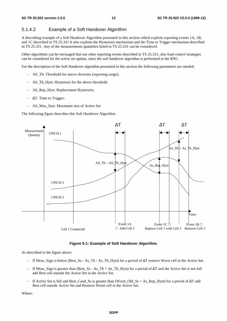
5.1.4.2 Example of a Soft Handover Algorithm

A describing example of a Soft Handover Algorithm presented in this section which exploits reporting events 1A, 1B,and 1C described in TS 25.331 It also exploits the Hysteresis mechanism and the Time to Trigger mechanism describedin TS 25.331. Any of the measurements quantities listed in TS 25.331 can be considered.

Other algorithms can be envisaged that use other reporting events described in TS 25.331; also load control strategiescan be considered for the active set update, since the soft handover algorithm is performed in the RNC.

For the description of the Soft Handover algorithm presented in this section the following parameters are needed:

- AS_Th: Threshold for macro diversity (reporting range);

- AS_Th_Hyst: Hysteresis for the above threshold;

- AS_Rep_Hyst: Replacement Hysteresis;

- ∆T: Time to Trigger;

- AS_Max_Size: Maximum size of Active Set

The following figure describes this Soft Handover Algorithm.

AS_Th – AS_Th_HystAs_Rep_Hyst

As_Th + As_Th_Hyst

Cell 1 Connected

Event 1A⇒ Add Cell 2

Event 1C ⇒Replace Cell 1 with Cell 3

Event 1B ⇒Remove Cell 3

CPICH 1

CPICH 2

CPICH 3

Time

MeasurementQuantity

∆T ∆T ∆T

Figure 5-1: Example of Soft Handover Algorithm.

As described in the figure above:

- If Meas_Sign is below (Best_Ss - As_Th - As_Th_Hyst) for a period of ∆T remove Worst cell in the Active Set.

- If Meas_Sign is greater than (Best_Ss - As_Th + As_Th_Hyst) for a period of ∆T and the Active Set is not fulladd Best cell outside the Active Set in the Active Set.

- If Active Set is full and Best_Cand_Ss is greater than (Worst_Old_Ss + As_Rep_Hyst) for a period of ∆T addBest cell outside Active Set and Remove Worst cell in the Active Set.

Where:

3GPP

3G TR 25.922 V2.0.0 (1999-12)133G TR 25.922 version 2.0.0

- Best_Ss :the best measured cell present in the Active Set;

- Worst_Old_Ss: the worst measured cell present in the Active Set;

- Best_Cand_Set:the best measured cell present in the monitored set .

- Meas_Sign :the measured and filtered quantity.

A flow-chart of the above described Soft Handover algorithm is available in Appendix C.

5.1.4.3 Soft Handover Execution

The Soft Handover is executed by means of the following procedures described in [6]:

- Radio Link Addition (FDD soft-add)

- Radio Link Removal (FDD soft-drop)

- Combined Radio Link Addition and Removal

The serving cell(s) (the cells in the active set) are expected to have knowledge of the service used by the UE. The newcell decided to be added to the active set shall be informed that a new connection is desired, and it needs to have thefollowing minimum information forwarded from the RNC:

- Connection parameters, such as coding schemes, number of parallel code channels etc. parameters which formthe set of parameters describing the different transport channel configurations in use both uplink and downlink.

- The UE ID and uplink scrambling code

- The relative timing information of the new cell, in respect to the timing UE is experiencing from the existingconnections (as measured by the UE at its location). Based on this, the new Node-B can determine what shouldbe the timing of the transmission initiated in respect to the timing of the common channels (CPICH) of the newcell.

As a response the UE needs to know via the existing connections:

- What channelisation code(s) are used for that transmission. The channelisation codes from different cells are notrequired to be the same as they are under different scrambling codes.

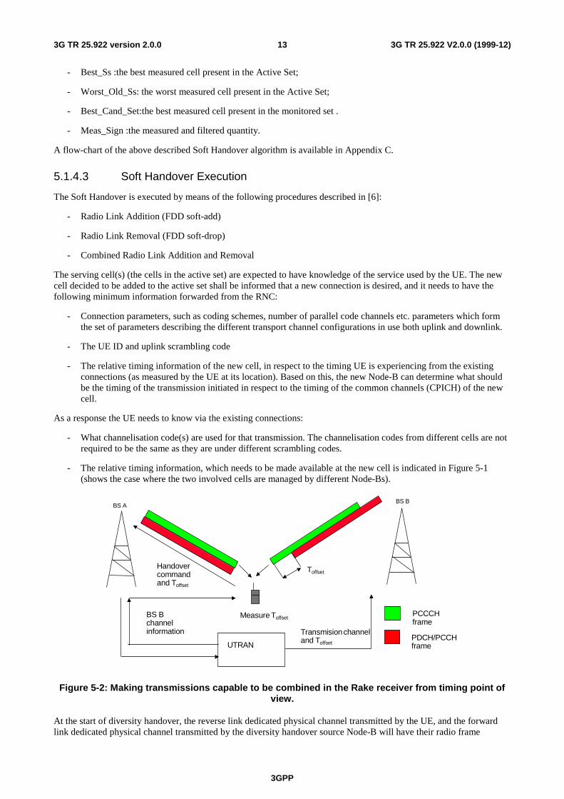
- The relative timing information, which needs to be made available at the new cell is indicated in Figure 5-1(shows the case where the two involved cells are managed by different Node-Bs).

PCCCHframe

PDCH/PCCHframe

Measure Toffset

Handovercommandand Toffset

UTRAN

Transmision channeland Toffset

BS Bchannelinformation

BS ABS B

Toffset

Figure 5-2: Making transmissions capable to be combined in the Rake receiver from timing point ofview.

At the start of diversity handover, the reverse link dedicated physical channel transmitted by the UE, and the forwardlink dedicated physical channel transmitted by the diversity handover source Node-B will have their radio frame

3GPP

3G TR 25.922 V2.0.0 (1999-12)143G TR 25.922 version 2.0.0

number and scrambling code phase counted up continuously as usual, and they will not change at all. Naturally, thecontinuity of the user information mounted on them will also be guaranteed, and will not cause any interruption.

5.1.5 Inter System Handover

5.1.5.1 Handover 3G to 2G

The handover from UTRA to GSM offering world-wide coverage already today has been one of the main design criteriataken into account in the UTRA frame timing definition.

The handover from UTRA/FDD to GSM can be implemented without simultaneous use of two receiver chains.Although the frame length is different from GSM frame length, the GSM traffic channel and UTRA FDD channels usesimilar multi-frame structure.

A UE can do the measurements by using idle periods in the downlink transmission, where such idle periods are createdby using the downlink Compressed Mode as defined in WG1 Specification. The Compressed Mode is under the controlof the UTRAN, and the UTRAN should communicate to the UE which frame is slotted.

Alternatively independent measurements not relying on the Compressed Mode, but using a dual receiver approach canbe performed, where the GSM receiver branch can operate independently of the UTRA FDD receiver branch.

The Handover from UTRA/TDD to GSM can be implemented without simultaneous use of two receiver chains.Although the frame length is different from GSM frame length, the GSM traffic channel and UTRA TDD channels relyon similar multi-frame structure.

A UE can do the measurements either by efficiently using idle slots or by getting assigned free continuous periods inthe downlink part obtained by reducing the spreading factor and compressing in time TS occupation in a form similar tothe FDD Compressed Mode. The low-cost constraint excludes the dual receiver approach.

For smooth inter-operation, inter-system information exchanges are needed in order to allow the UTRAN to notify theUE of the existing GSM frequencies in the area and vice versa. Further more integrated operation is needed for theactual handover where the current service is maintained, taking naturally into account the lower data rate capabilities inGSM when compared to UMTS maximum data rates reaching all the way to 2 Mbits/s.

5.1.6 Measurements for Handover

5.1.6.1 Monitoring of FDD cells on the same frequency

During the measurement process of cells on the same frequencies, the UE shall find the necessary synchronisation to thecells to measure using the primary and secondary synchronisation channels and also the knowledge of the possiblescrambling codes in use by the neighbouring cells.

5.1.6.2 Monitoring cells on different frequencies

5.1.6.2.1 Monitoring of FDD cells on a different frequency

Upper layers may ask FDD UE to perform preparation of inter-frequency handover to FDD. In such case, the UTRANsignals to the UE the handover monitoring set, and if needed, the compressed mode parameters used to make the neededmeasurements. Setting of the compressed mode parameters defined in [3] for the preparation of handover from UTRAFDD to UTRA FDD is indicated in the following section. The compressed mode for IFHO preparation from UTRA-FDD to UTRA-FDD has two different modes. One is "selection-mode". The UE must identify the cell during this mode.The other is "reselection-mode". The UE measures signal strength by the scrambling code already known. Selectionmode / reselection mode parameter sets are described in section 5.6.1.2.1.1/5.6.1.2.1.2 respectively.

Measurements to be performed by the physical layer are defined in [3]

5.1.6.2.1.1 Setting of the compressed mode parameters for selection mode

During the transmission gaps, the UE shall perform measurements so as to be able to report to the UTRAN the frametiming, the scrambling code and the Ec/Io of Primary CCPCH of up FDD cells in the handover monitoring set.

3GPP

3G TR 25.922 V2.0.0 (1999-12)153G TR 25.922 version 2.0.0

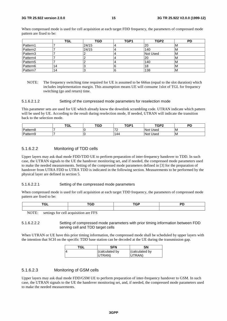
When compressed mode is used for cell acquisition at each target FDD frequency, the parameters of compressed modepattern are fixed to be:

TGL TGD TGP1 TGP2 PDPattern1 7 24/15 4 20 MPattern2 7 24/15 4 140 MPattern3 7 2 4 Not Used MPattern4 7 2 4 20 MPattern5 7 2 4 140 MPattern6 14 3 6 18 MPattern7 14 3 6 138 M

NOTE: The frequency switching time required for UE is assumed to be 666us (equal to the slot duration) whichincludes implementation margin. This assumption means UE will consume 1slot of TGL for frequencyswitching (go and return) time.

5.1.6.2.1.2 Setting of the compressed mode parameters for reselection mode

This parameter sets are used for UE which already know the downlink scrambling code. UTRAN indicate which patternwill be used by UE. According to the result during reselection mode, If needed, UTRAN will indicate the transitionback to the selection mode.

TGL TGD TGP1 TGP2 PDPattern8 7 0 72 Not Used MPattern9 7 0 144 Not Used M

5.1.6.2.2 Monitoring of TDD cells

Upper layers may ask dual mode FDD/TDD UE to perform preparation of inter-frequency handover to TDD. In suchcase, the UTRAN signals to the UE the handover monitoring set, and if needed, the compressed mode parameters usedto make the needed measurements. Setting of the compressed mode parameters defined in [3] for the preparation ofhandover from UTRA FDD to UTRA TDD is indicated in the following section. Measurements to be performed by thephysical layer are defined in section 5.

5.1.6.2.2.1 Setting of the compressed mode parameters

When compressed mode is used for cell acquisition at each target TDD frequency, the parameters of compressed modepattern are fixed to be:

TGL TGD TGP PD

NOTE: settings for cell acquisition are FFS

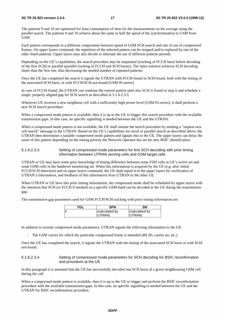
5.1.6.2.2.2 Setting of compressed mode parameters with prior timing information between FDDserving cell and TDD target cells

When UTRAN or UE have this prior timing information, the compressed mode shall be scheduled by upper layers withthe intention that SCH on the specific TDD base station can be decoded at the UE during the transmission gap.

TGL SFN SN4 (calculated by

UTRAN)(calculated byUTRAN)

5.1.6.2.3 Monitoring of GSM cells

Upper layers may ask dual mode FDD/GSM UE to perform preparation of inter-frequency handover to GSM. In suchcase, the UTRAN signals to the UE the handover monitoring set, and, if needed, the compressed mode parameters usedto make the needed measurements.

3GPP

3G TR 25.922 V2.0.0 (1999-12)163G TR 25.922 version 2.0.0

The involved measurements are GSM BCCH power measurements (Section 5.1.6.2.3.1), initial GSM SCH or FCCHacquisition (Section 5.1.6.2.3.2), acquisition/tracking of GSM SCH or FCCH when timing information between UTRAserving cells and the target GSM cell is available (Section 5.1.6.2.3.3), and BSIC reconfirmation (Section 5.1.6.2.3.4).

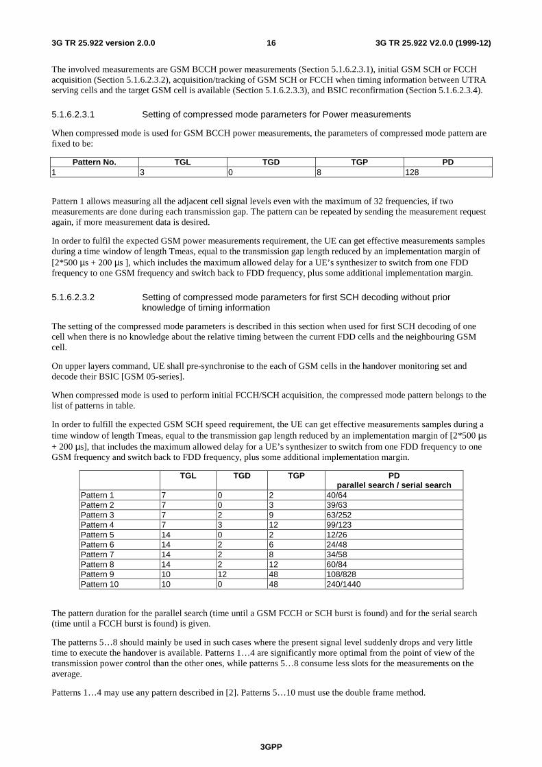
5.1.6.2.3.1 Setting of compressed mode parameters for Power measurements

When compressed mode is used for GSM BCCH power measurements, the parameters of compressed mode pattern arefixed to be:

Pattern No. TGL TGD TGP PD1 3 0 8 128

Pattern 1 allows measuring all the adjacent cell signal levels even with the maximum of 32 frequencies, if twomeasurements are done during each transmission gap. The pattern can be repeated by sending the measurement requestagain, if more measurement data is desired.

In order to fulfil the expected GSM power measurements requirement, the UE can get effective measurements samplesduring a time window of length Tmeas, equal to the transmission gap length reduced by an implementation margin of[2*500 µs + 200 µs ], which includes the maximum allowed delay for a UE’s synthesizer to switch from one FDDfrequency to one GSM frequency and switch back to FDD frequency, plus some additional implementation margin.

5.1.6.2.3.2 Setting of compressed mode parameters for first SCH decoding without priorknowledge of timing information

The setting of the compressed mode parameters is described in this section when used for first SCH decoding of onecell when there is no knowledge about the relative timing between the current FDD cells and the neighbouring GSMcell.

On upper layers command, UE shall pre-synchronise to the each of GSM cells in the handover monitoring set anddecode their BSIC [GSM 05-series].

When compressed mode is used to perform initial FCCH/SCH acquisition, the compressed mode pattern belongs to thelist of patterns in table.

In order to fulfill the expected GSM SCH speed requirement, the UE can get effective measurements samples during atime window of length Tmeas, equal to the transmission gap length reduced by an implementation margin of [2*500 µs+ 200 µs], that includes the maximum allowed delay for a UE’s synthesizer to switch from one FDD frequency to oneGSM frequency and switch back to FDD frequency, plus some additional implementation margin.

TGL TGD TGP PDparallel search / serial search

Pattern 1 7 0 2 40/64Pattern 2 7 0 3 39/63Pattern 3 7 2 9 63/252Pattern 4 7 3 12 99/123Pattern 5 14 0 2 12/26Pattern 6 14 2 6 24/48Pattern 7 14 2 8 34/58Pattern 8 14 2 12 60/84Pattern 9 10 12 48 108/828Pattern 10 10 0 48 240/1440

The pattern duration for the parallel search (time until a GSM FCCH or SCH burst is found) and for the serial search(time until a FCCH burst is found) is given.

The patterns 5…8 should mainly be used in such cases where the present signal level suddenly drops and very littletime to execute the handover is available. Patterns 1…4 are significantly more optimal from the point of view of thetransmission power control than the other ones, while patterns 5…8 consume less slots for the measurements on theaverage.

Patterns 1…4 may use any pattern described in [2]. Patterns 5…10 must use the double frame method.

3GPP

3G TR 25.922 V2.0.0 (1999-12)173G TR 25.922 version 2.0.0

The patterns 9 and 10 are optimised for least consumption of slots for the measurements on the average using theparallel search. The patterns 9 and 10 achieve about the same or half the speed of the synchronisation to GSM fromGSM.

Each pattern corresponds to a different compromise between speed of GSM SCH search and rate of use of compressedframes. On upper layers command, the repetition of the selected pattern can be stopped and/or replaced by one of theother listed patterns. Upper layers may also decide to alternate the use of different patterns periods.

Depending on the UE’s capabilities, the search procedure may be sequential (tracking of FCCH burst before decodingof the first SCH) or parallel (parallel tracking of FCCH and SCH bursts). The latter solution achieves SCH decodingfaster than the first one, thus decreasing the needed number of repeated patterns.

Once the UE has completed the search it signals the UTRAN with FCCH-found or SCH-found, both with the timing ofthe associated SCH burst, or with FCCH/SCH-not-found [GSM 05-series].

In case of FCCH-found, the UTRAN can continue the current pattern until also SCH is found or stop it and schedule asingle, properly aligned gap for SCH search as described in 5.1.6.2.3.3.

Whenever UE receives a new neighbour cell with a sufficiently high power level [GSM 05-series], it shall perform anew SCH search procedure.

When a compressed mode pattern is available, then it is up to the UE to trigger this search procedure with the availabletransmission gaps. In this case, no specific signalling is needed between the UE and the UTRAN.

When a compressed mode pattern is not available, the UE shall initiate the search procedure by sending a "request newcell search" message to the UTRAN. Based on the UE’s capabilities for serial or parallel search as described above, theUTRAN then determines a suitable compressed mode pattern and signals this to the UE. The upper layers can delay theonset of this pattern depending on the timing priority the Network Operator has set for new BSIC identification.

5.1.6.2.3.3 Setting of compressed mode parameters for first SCH decoding with prior timinginformation between UTRAN serving cells and GSM target cells

UTRAN or UE may have some prior knowledge of timing difference between some FDD cells in UE’s active set andsome GSM cells in the handover monitoring set. When this information is acquired by the UE (e.g. after initialFCCH/SCH detection) and on upper layers command, the UE shall report it to the upper layers for verification ofUTRAN’s information, and feedback of this information from UTRAN to the other UE.

When UTRAN or UE have this prior timing information, the compressed mode shall be scheduled by upper layers withthe intention that SCH (or FCCH if needed) on a specific GSM band can be decoded at the UE during the transmissiongap.

The transmission gap parameters used for GSM FCCH/SCH tracking with prior timing information are:

TGL SFN SN4 (calculated by

UTRAN)(calculated byUTRAN)

In addition to normal compressed mode parameters, UTRAN signals the following information to the UE:

- The GSM carrier for which the particular compressed frame is intended (BS ID, carrier no, etc.)

Once the UE has completed the search, it signals the UTRAN with the timing of the associated SCH burst or with SCH-not-found.

5.1.6.2.3.4 Setting of compressed mode parameters for SCH decoding for BSIC reconfirmationand procedure at the UE

In this paragraph it is assumed that the UE has successfully decoded one SCH burst of a given neighbouring GSM cellduring the call.

When a compressed mode pattern is available, then it is up to the UE to trigger and perform the BSIC reconfirmationprocedure with the available transmission gaps. In this case, no specific signalling is needed between the UE and theUTRAN for BSIC reconfirmation procedure.

3GPP

3G TR 25.922 V2.0.0 (1999-12)183G TR 25.922 version 2.0.0

When no compressed mode pattern is available then it is up to the UE to trigger and perform the BSIC reconfirmationprocedure. In that case, UE indicates to the upper layers the schedule of the SCH burst of that cell, and the size of thenecessary transmission gap necessary to capture one SCH burst. The Network Operator decides the target time for BSICreconfirmation and the upper layers uses this and the schedule indicated by the UE to determine the appropriatecompressed mode parameters.

The compressed mode parameters shall be one of those described in [3].

5.1.6.2.3.5 Parametrisation of the compressed mode for handover preparation to GSM

Whereas section 5.1.6.2.3.2 described the compressed mode parametrisation for the initial synchronisation tracking orreconfirmation for one cell and the compressed mode parameters for power measurement for one of multiple cells, thereis a need to define the global compressed mode parameters when considering the monitoring of all GSM cells.

6 Admission Control

6.1 IntroductionIn CDMA networks the 'soft capacity' concept applies: each new call increases the interference level of all otherongoing calls, affecting their quality. Therefore it is very important to control the access to the network in a suitableway (Call Admission Control - CAC).

6.2 Examples of CAC strategiesPrinciple 1: Admission Control is performed according to the type of required QoS.

"Type of service" is to be understood as an implementation specific category derived from standardized QoSparameters.

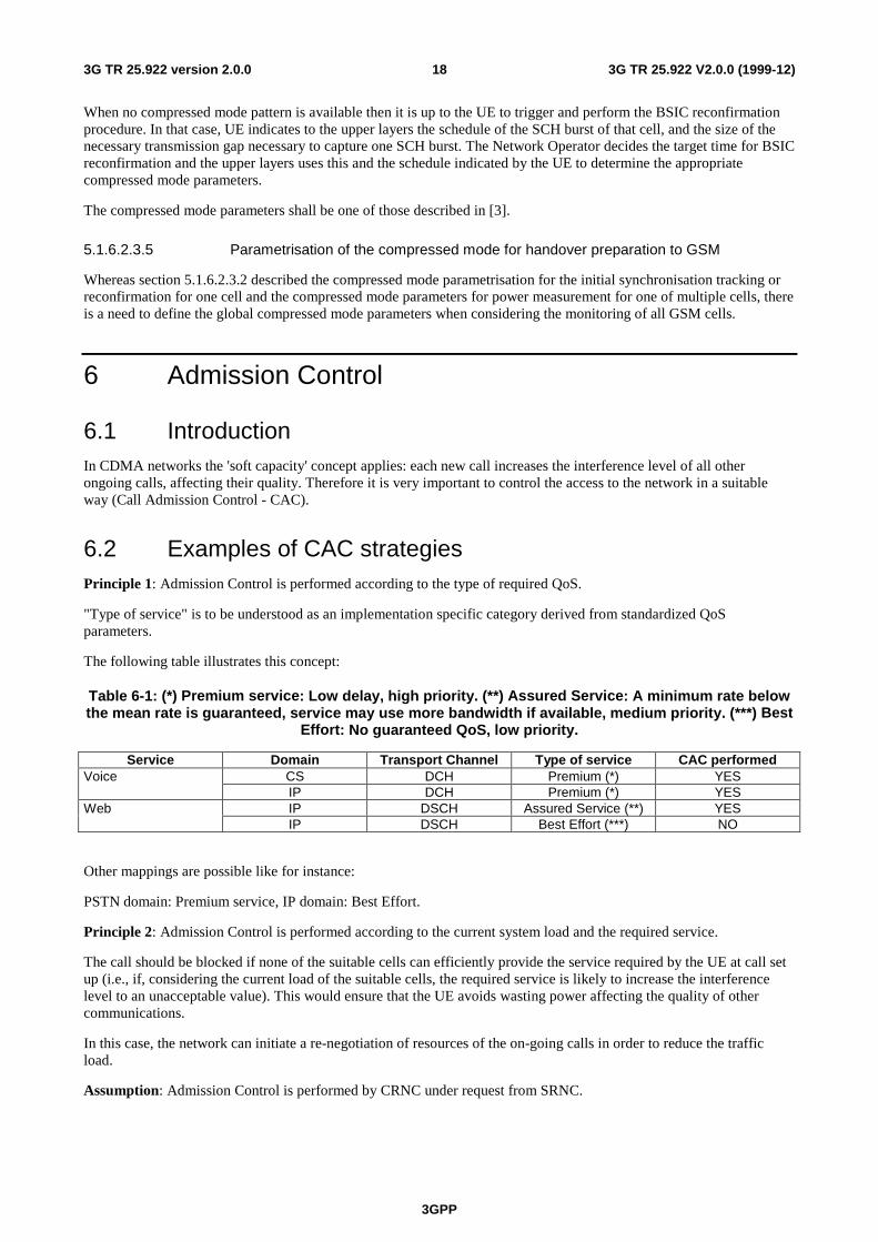
The following table illustrates this concept:

Table 6-1: (*) Premium service: Low delay, high priority. (**) Assured Service: A minimum rate belowthe mean rate is guaranteed, service may use more bandwidth if available, medium priority. (***) Best

Effort: No guaranteed QoS, low priority.

Service Domain Transport Channel Type of service CAC performedCS DCH Premium (*) YESVoiceIP DCH Premium (*) YESIP DSCH Assured Service (**) YESWebIP DSCH Best Effort (***) NO

Other mappings are possible like for instance:

PSTN domain: Premium service, IP domain: Best Effort.

Principle 2: Admission Control is performed according to the current system load and the required service.

The call should be blocked if none of the suitable cells can efficiently provide the service required by the UE at call setup (i.e., if, considering the current load of the suitable cells, the required service is likely to increase the interferencelevel to an unacceptable value). This would ensure that the UE avoids wasting power affecting the quality of othercommunications.

In this case, the network can initiate a re-negotiation of resources of the on-going calls in order to reduce the trafficload.

Assumption: Admission Control is performed by CRNC under request from SRNC.

3GPP

3G TR 25.922 V2.0.0 (1999-12)193G TR 25.922 version 2.0.0

6.3 Scenarios

6.3.1 CAC performed in SRNC

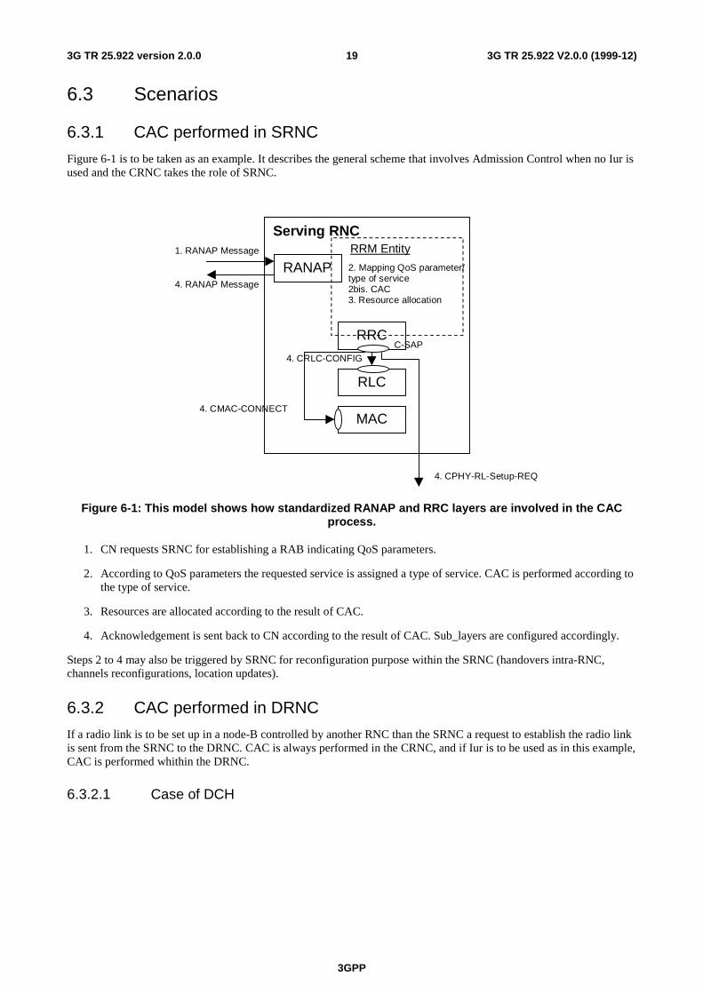
Figure 6-1 is to be taken as an example. It describes the general scheme that involves Admission Control when no Iur isused and the CRNC takes the role of SRNC.

Serving RNC

RANAP

RRC

RRM Entity

4. CPHY-RL-Setup-REQ

C-SAP

1. RANAP Message

4. RANAP Message

2. Mapping QoS parameter/type of service2bis. CAC3. Resource allocation

MAC4. CMAC-CONNECT

RLC

4. CRLC-CONFIG

Figure 6-1: This model shows how standardized RANAP and RRC layers are involved in the CACprocess.

1. CN requests SRNC for establishing a RAB indicating QoS parameters.

2. According to QoS parameters the requested service is assigned a type of service. CAC is performed according tothe type of service.

3. Resources are allocated according to the result of CAC.

4. Acknowledgement is sent back to CN according to the result of CAC. Sub_layers are configured accordingly.

Steps 2 to 4 may also be triggered by SRNC for reconfiguration purpose within the SRNC (handovers intra-RNC,channels reconfigurations, location updates).

6.3.2 CAC performed in DRNC

If a radio link is to be set up in a node-B controlled by another RNC than the SRNC a request to establish the radio linkis sent from the SRNC to the DRNC. CAC is always performed in the CRNC, and if Iur is to be used as in this example,CAC is performed whithin the DRNC.

6.3.2.1 Case of DCH

3GPP

3G TR 25.922 V2.0.0 (1999-12)203G TR 25.922 version 2.0.0

Drift RNC

RNSAP

RRC

RRM Entity


C- SAP

1. RNSAP Message

4. RNSAP Message

2. CAC3. Resource allocation

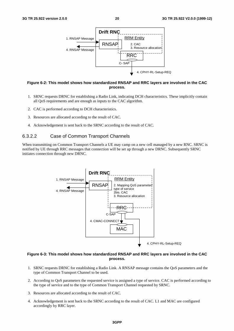
Figure 6-2: This model shows how standardized RNSAP and RRC layers are involved in the CACprocess.

1. SRNC requests DRNC for establishing a Radio Link, indicating DCH characteristics. These implicitly containall QoS requirements and are enough as inputs to the CAC algorithm.

2. CAC is performed according to DCH characteristics.


4. Acknowledgement is sent back to the SRNC according to the result of CAC.

6.3.2.2 Case of Common Transport Channels

When transmitting on Common Transport Channels a UE may camp on a new cell managed by a new RNC. SRNC isnotified by UE through RRC messages that connection will be set up through a new DRNC. Subsequently SRNCinitiates connection through new DRNC.

Drift RNC

RNSAP

RRC

RRM Entity


C-SAP

1. RNSAP Message

4. RNSAP Message

2. Mapping QoS parameter/type of service2bis. CAC3. Resource allocation

MAC

4. CMAC-CONNECT

Figure 6-3: This model shows how standardized RNSAP and RRC layers are involved in the CACprocess.

1. SRNC requests DRNC for establishing a Radio Link. A RNSAP message contains the QoS parameters and thetype of Common Transport Channel to be used.

2. According to QoS parameters the requested service is assigned a type of service. CAC is performed according tothe type of service and to the type of Common Transport Channel requested by SRNC.


4. Acknowledgement is sent back to the SRNC according to the result of CAC. L1 and MAC are configuredaccordingly by RRC layer.

3GPP

3G TR 25.922 V2.0.0 (1999-12)213G TR 25.922 version 2.0.0

7 Radio Bearer Control

7.1 Usage of Radio Bearer Control proceduresRadio Bearer (RB) Control procedures are used to control the UE and system resources. This section explains how thesystem works with respect to these procedures and how e.g. traffic volume measurements could trigger theseprocedures.

7.1.1 Examples of Radio Bearer Setup

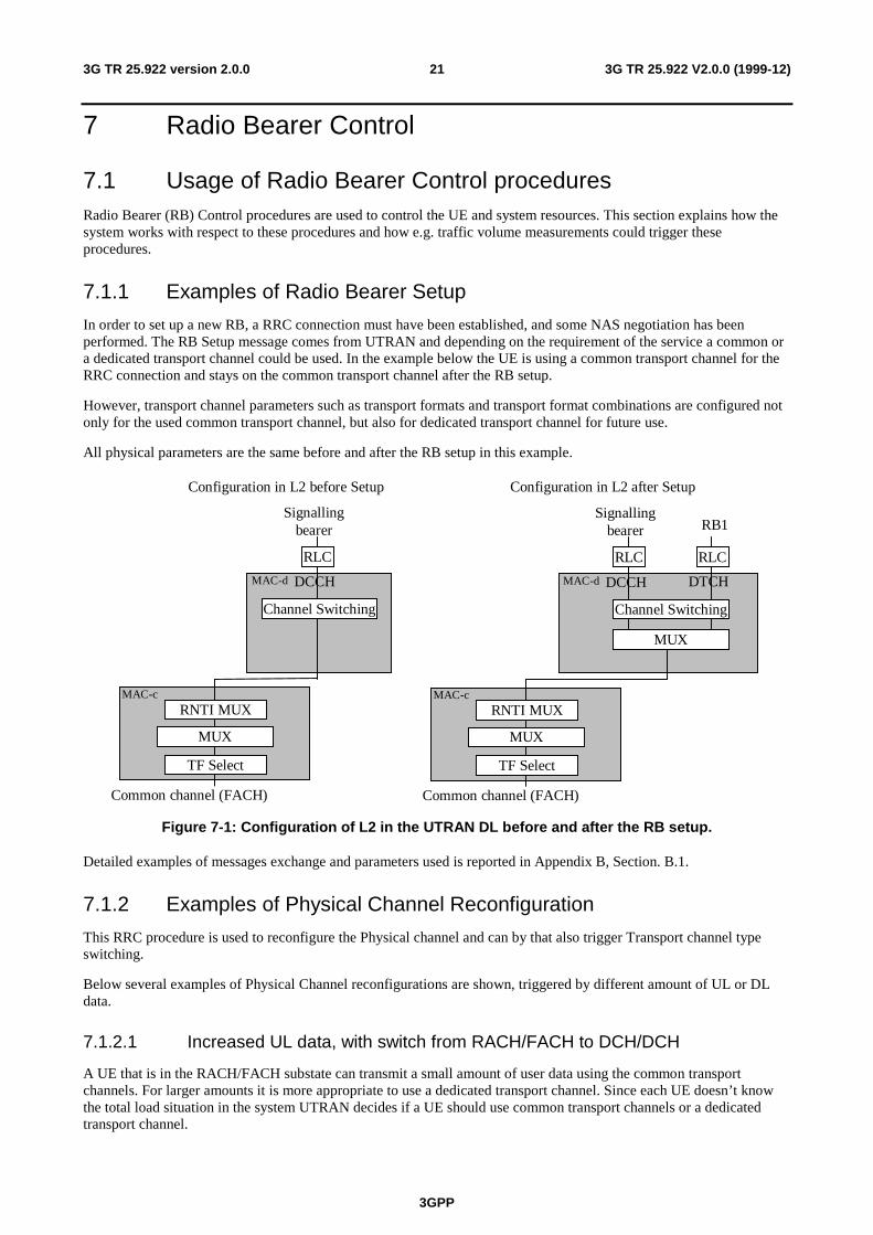
In order to set up a new RB, a RRC connection must have been established, and some NAS negotiation has beenperformed. The RB Setup message comes from UTRAN and depending on the requirement of the service a common ora dedicated transport channel could be used. In the example below the UE is using a common transport channel for theRRC connection and stays on the common transport channel after the RB setup.

However, transport channel parameters such as transport formats and transport format combinations are configured notonly for the used common transport channel, but also for dedicated transport channel for future use.

All physical parameters are the same before and after the RB setup in this example.

MAC-c

MAC-d

Configuration in L2 before Setup

RLC

TF Select

Common channel (FACH)

Channel Switching

Configuration in L2 after Setup

RNTI MUX

Signallingbearer

DCCH

MUX

MAC-c

MAC-d

RLC

TF Select


RLC

Channel Switching

MUX

RNTI MUX

Signallingbearer RB1

DCCH DTCH

MUX

Figure 7-1: Configuration of L2 in the UTRAN DL before and after the RB setup.

Detailed examples of messages exchange and parameters used is reported in Appendix B, Section. B.1.

7.1.2 Examples of Physical Channel Reconfiguration

This RRC procedure is used to reconfigure the Physical channel and can by that also trigger Transport channel typeswitching.

Below several examples of Physical Channel reconfigurations are shown, triggered by different amount of UL or DLdata.

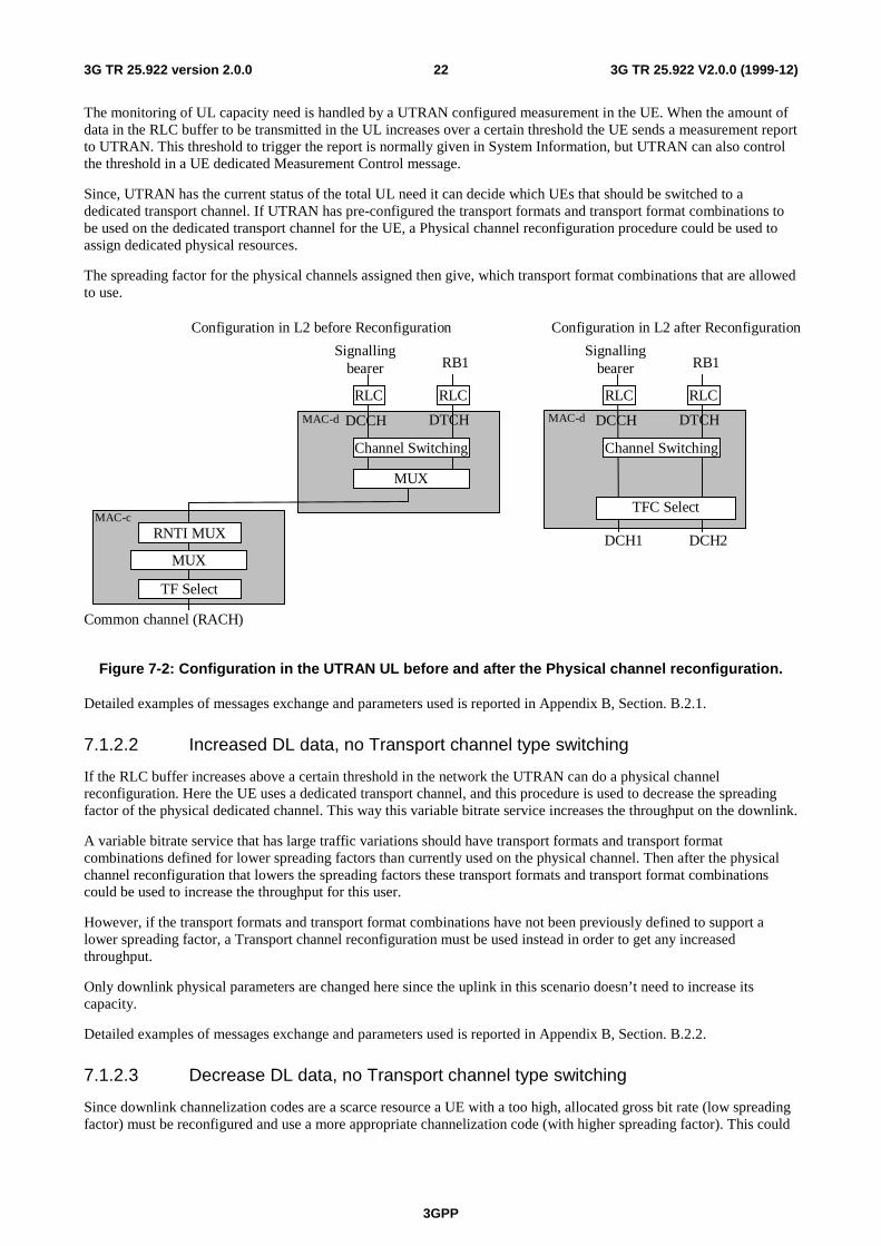
7.1.2.1 Increased UL data, with switch from RACH/FACH to DCH/DCH

A UE that is in the RACH/FACH substate can transmit a small amount of user data using the common transportchannels. For larger amounts it is more appropriate to use a dedicated transport channel. Since each UE doesn’t knowthe total load situation in the system UTRAN decides if a UE should use common transport channels or a dedicatedtransport channel.

3GPP

3G TR 25.922 V2.0.0 (1999-12)223G TR 25.922 version 2.0.0

The monitoring of UL capacity need is handled by a UTRAN configured measurement in the UE. When the amount ofdata in the RLC buffer to be transmitted in the UL increases over a certain threshold the UE sends a measurement reportto UTRAN. This threshold to trigger the report is normally given in System Information, but UTRAN can also controlthe threshold in a UE dedicated Measurement Control message.

Since, UTRAN has the current status of the total UL need it can decide which UEs that should be switched to adedicated transport channel. If UTRAN has pre-configured the transport formats and transport format combinations tobe used on the dedicated transport channel for the UE, a Physical channel reconfiguration procedure could be used toassign dedicated physical resources.

The spreading factor for the physical channels assigned then give, which transport format combinations that are allowedto use.

MAC-c

MAC-d MAC-d

Configuration in L2 before Reconfiguration

RLC

TF Select

Common channel (RACH)

RLC

Channel Switching

MUX

Configuration in L2 after Reconfiguration

RLC

DCH1

RLC

TFC Select

DCH2

Channel Switching

RNTI MUX


DCCH DTCH


DCCH DTCH

MUX

Figure 7-2: Configuration in the UTRAN UL before and after the Physical channel reconfiguration.

Detailed examples of messages exchange and parameters used is reported in Appendix B, Section. B.2.1.

7.1.2.2 Increased DL data, no Transport channel type switching

If the RLC buffer increases above a certain threshold in the network the UTRAN can do a physical channelreconfiguration. Here the UE uses a dedicated transport channel, and this procedure is used to decrease the spreadingfactor of the physical dedicated channel. This way this variable bitrate service increases the throughput on the downlink.

A variable bitrate service that has large traffic variations should have transport formats and transport formatcombinations defined for lower spreading factors than currently used on the physical channel. Then after the physicalchannel reconfiguration that lowers the spreading factors these transport formats and transport format combinationscould be used to increase the throughput for this user.

However, if the transport formats and transport format combinations have not been previously defined to support alower spreading factor, a Transport channel reconfiguration must be used instead in order to get any increasedthroughput.

Only downlink physical parameters are changed here since the uplink in this scenario doesn’t need to increase itscapacity.


7.1.2.3 Decrease DL data, no Transport channel type switching

Since downlink channelization codes are a scarce resource a UE with a too high, allocated gross bit rate (low spreadingfactor) must be reconfigured and use a more appropriate channelization code (with higher spreading factor). This could

3GPP

3G TR 25.922 V2.0.0 (1999-12)233G TR 25.922 version 2.0.0

be triggered by a threshold for the RLC buffer content and some inactivity timer, i.e. that the buffer content stays acertain time below this threshold

After the physical channel has been reconfigured, some of the transport formats and transport format combinations thatrequire a low SF can not be used. However, these are stored and could be used if the physical channel is reconfiguredlater to use a lower spreading factor.

Detailed examples of messages exchange and parameters used is reported in Appendix B, Section B.2.3.

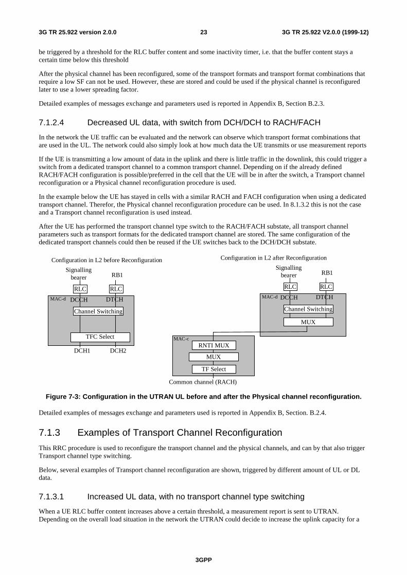
7.1.2.4 Decreased UL data, with switch from DCH/DCH to RACH/FACH

In the network the UE traffic can be evaluated and the network can observe which transport format combinations thatare used in the UL. The network could also simply look at how much data the UE transmits or use measurement reports

If the UE is transmitting a low amount of data in the uplink and there is little traffic in the downlink, this could trigger aswitch from a dedicated transport channel to a common transport channel. Depending on if the already definedRACH/FACH configuration is possible/preferred in the cell that the UE will be in after the switch, a Transport channelreconfiguration or a Physical channel reconfiguration procedure is used.

In the example below the UE has stayed in cells with a similar RACH and FACH configuration when using a dedicatedtransport channel. Therefor, the Physical channel reconfiguration procedure can be used. In 8.1.3.2 this is not the caseand a Transport channel reconfiguration is used instead.

After the UE has performed the transport channel type switch to the RACH/FACH substate, all transport channelparameters such as transport formats for the dedicated transport channel are stored. The same configuration of thededicated transport channels could then be reused if the UE switches back to the DCH/DCH substate.

MAC-c

MAC-dMAC-d


RLC

TF Select

Common channel (RACH)

RLC

Channel Switching

MUX


RLC

DCH1

RLC

TFC Select

DCH2

Channel Switching

RNTI MUX


DCCH DTCH


DCCH DTCH

MUX

Figure 7-3: Configuration in the UTRAN UL before and after the Physical channel reconfiguration.


7.1.3 Examples of Transport Channel Reconfiguration

This RRC procedure is used to reconfigure the transport channel and the physical channels, and can by that also triggerTransport channel type switching.

Below, several examples of Transport channel reconfiguration are shown, triggered by different amount of UL or DLdata.

7.1.3.1 Increased UL data, with no transport channel type switching

When a UE RLC buffer content increases above a certain threshold, a measurement report is sent to UTRAN.Depending on the overall load situation in the network the UTRAN could decide to increase the uplink capacity for a

3GPP

3G TR 25.922 V2.0.0 (1999-12)243G TR 25.922 version 2.0.0

UE. Since every UE has its "own" code tree, there is no shortage of UL codes with a low spreading factor, and all UEscan have a low spreading factor code allocated.

Therefore, instead of channelization code assignment as used in the DL, load control in the UL is handled by theallowed transport formats and transport format combinations for each UE. To increase the throughput for a UE in theuplink, UTRAN could send a Transport channel reconfiguration or a TFC Control message.

Here a Transport channel reconfiguration is used. Although, the TFC Control procedure is believed to require lesssignalling it can only restrict or remove restrictions of the assigned transport format combinations and that may notalways be enough. If a reconfiguration of the actual transport formats or transport format combinations is required, theTransport channel reconfiguration procedure must be used instead.

In the example below, the UE is allowed to send more data in the UL when on dedicated transport channel, although thecommon transport channel configuration is still the same. To make use of the new transport format combinations thephysical channel must also be reconfigured to allow a lower spreading factor.


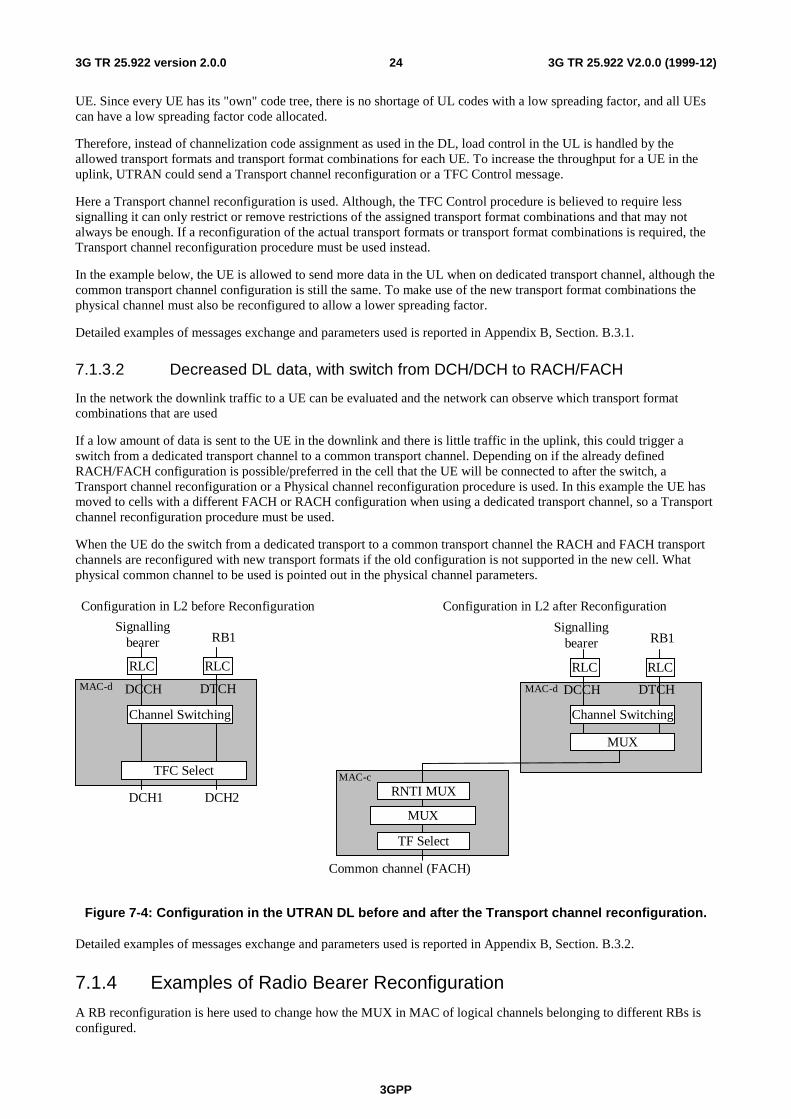
7.1.3.2 Decreased DL data, with switch from DCH/DCH to RACH/FACH

In the network the downlink traffic to a UE can be evaluated and the network can observe which transport formatcombinations that are used

If a low amount of data is sent to the UE in the downlink and there is little traffic in the uplink, this could trigger aswitch from a dedicated transport channel to a common transport channel. Depending on if the already definedRACH/FACH configuration is possible/preferred in the cell that the UE will be connected to after the switch, aTransport channel reconfiguration or a Physical channel reconfiguration procedure is used. In this example the UE hasmoved to cells with a different FACH or RACH configuration when using a dedicated transport channel, so a Transportchannel reconfiguration procedure must be used.

When the UE do the switch from a dedicated transport to a common transport channel the RACH and FACH transportchannels are reconfigured with new transport formats if the old configuration is not supported in the new cell. Whatphysical common channel to be used is pointed out in the physical channel parameters.

MAC-d


RLC

DCH1

RLC

TFC Select

DCH2

Channel Switching


DCCH DTCH

MAC-c

MAC-d


RLC

TF Select


RLC

Channel Switching

MUX

RNTI MUX


DCCH DTCH

MUX

Figure 7-4: Configuration in the UTRAN DL before and after the Transport channel reconfiguration.


7.1.4 Examples of Radio Bearer Reconfiguration

A RB reconfiguration is here used to change how the MUX in MAC of logical channels belonging to different RBs isconfigured.

3GPP

3G TR 25.922 V2.0.0 (1999-12)253G TR 25.922 version 2.0.0

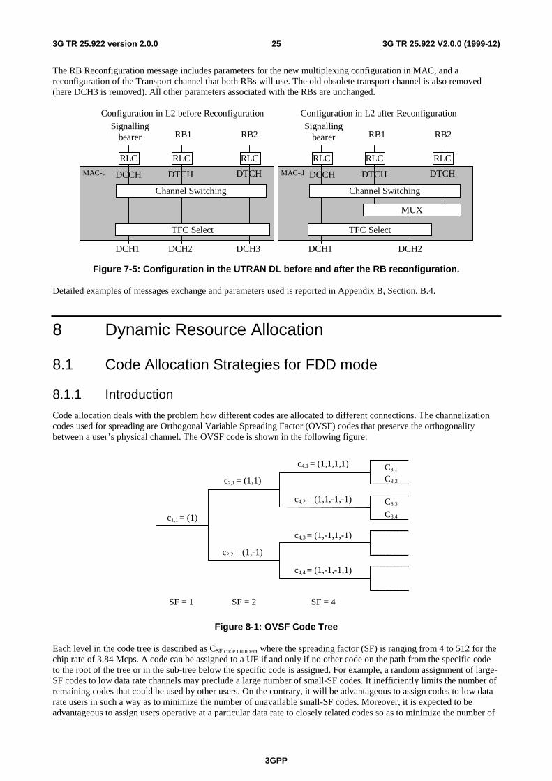
The RB Reconfiguration message includes parameters for the new multiplexing configuration in MAC, and areconfiguration of the Transport channel that both RBs will use. The old obsolete transport channel is also removed(here DCH3 is removed). All other parameters associated with the RBs are unchanged.

MAC-dMAC-d


RLC

DCH1

RLC

DCH2

RLC

TFC Select

DCH3

Channel Switching


RLC

DCH1

RLC

TFC Select

RLC

Channel Switching

MUX

DCH2


DCCH DTCH

RB2

DTCH


DCCH DTCH

RB2

DTCH

Figure 7-5: Configuration in the UTRAN DL before and after the RB reconfiguration.

Detailed examples of messages exchange and parameters used is reported in Appendix B, Section. B.4.

8 Dynamic Resource Allocation

8.1 Code Allocation Strategies for FDD mode

8.1.1 Introduction

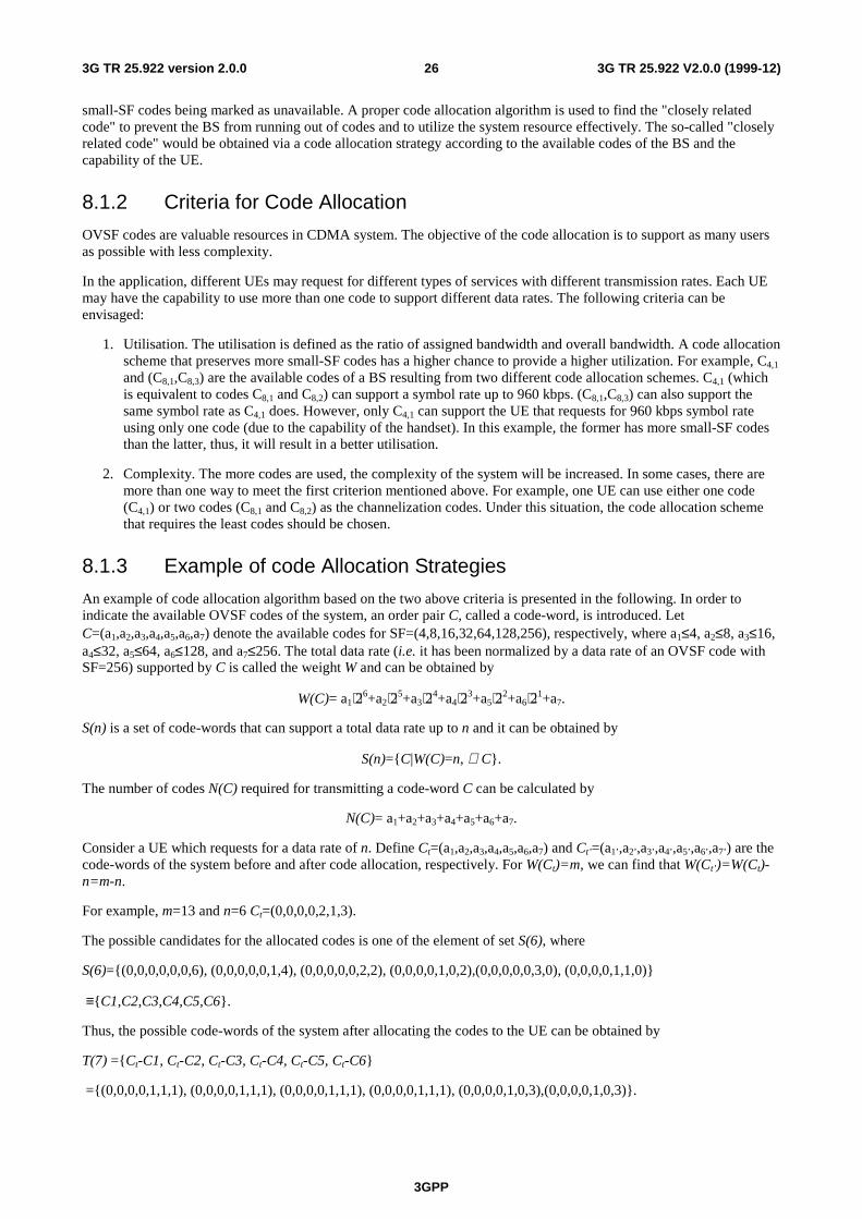
Code allocation deals with the problem how different codes are allocated to different connections. The channelizationcodes used for spreading are Orthogonal Variable Spreading Factor (OVSF) codes that preserve the orthogonalitybetween a user’s physical channel. The OVSF code is shown in the following figure:

SF = 1 SF = 2 SF = 4

c1,1 = (1)

c2,1 = (1,1)

c2,2 = (1,-1)

c4,1 = (1,1,1,1)

c4,2 = (1,1,-1,-1)

c4,3 = (1,-1,1,-1)

c4,4 = (1,-1,-1,1)

C8,1

C8,2

C8,3

C8,4

Figure 8-1: OVSF Code Tree

Each level in the code tree is described as CSF,code number, where the spreading factor (SF) is ranging from 4 to 512 for thechip rate of 3.84 Mcps. A code can be assigned to a UE if and only if no other code on the path from the specific codeto the root of the tree or in the sub-tree below the specific code is assigned. For example, a random assignment of large-SF codes to low data rate channels may preclude a large number of small-SF codes. It inefficiently limits the number ofremaining codes that could be used by other users. On the contrary, it will be advantageous to assign codes to low datarate users in such a way as to minimize the number of unavailable small-SF codes. Moreover, it is expected to beadvantageous to assign users operative at a particular data rate to closely related codes so as to minimize the number of

3GPP

3G TR 25.922 V2.0.0 (1999-12)263G TR 25.922 version 2.0.0

small-SF codes being marked as unavailable. A proper code allocation algorithm is used to find the "closely relatedcode" to prevent the BS from running out of codes and to utilize the system resource effectively. The so-called "closelyrelated code" would be obtained via a code allocation strategy according to the available codes of the BS and thecapability of the UE.

8.1.2 Criteria for Code Allocation

OVSF codes are valuable resources in CDMA system. The objective of the code allocation is to support as many usersas possible with less complexity.

In the application, different UEs may request for different types of services with different transmission rates. Each UEmay have the capability to use more than one code to support different data rates. The following criteria can beenvisaged:

1. Utilisation. The utilisation is defined as the ratio of assigned bandwidth and overall bandwidth. A code allocationscheme that preserves more small-SF codes has a higher chance to provide a higher utilization. For example, C4,1

and (C8,1,C8,3) are the available codes of a BS resulting from two different code allocation schemes. C4,1 (whichis equivalent to codes C8,1 and C8,2) can support a symbol rate up to 960 kbps. (C8,1,C8,3) can also support thesame symbol rate as C4,1 does. However, only C4,1 can support the UE that requests for 960 kbps symbol rateusing only one code (due to the capability of the handset). In this example, the former has more small-SF codesthan the latter, thus, it will result in a better utilisation.

2. Complexity. The more codes are used, the complexity of the system will be increased. In some cases, there aremore than one way to meet the first criterion mentioned above. For example, one UE can use either one code(C4,1) or two codes (C8,1 and C8,2) as the channelization codes. Under this situation, the code allocation schemethat requires the least codes should be chosen.

8.1.3 Example of code Allocation Strategies

An example of code allocation algorithm based on the two above criteria is presented in the following. In order toindicate the available OVSF codes of the system, an order pair C, called a code-word, is introduced. LetC=(a1,a2,a3,a4,a5,a6,a7) denote the available codes for SF=(4,8,16,32,64,128,256), respectively, where a1≤4, a2≤8, a3≤16,a4≤32, a5≤64, a6≤128, and a7≤256. The total data rate (i.e. it has been normalized by a data rate of an OVSF code withSF=256) supported by C is called the weight W and can be obtained by

W(C)= a1⋅26+a2⋅25+a3⋅24+a4⋅23+a5⋅22+a6⋅21+a7.

S(n) is a set of code-words that can support a total data rate up to n and it can be obtained by

S(n)={C|W(C)=n, ∀ C}.

The number of codes N(C) required for transmitting a code-word C can be calculated by

N(C)= a1+a2+a3+a4+a5+a6+a7.

Consider a UE which requests for a data rate of n. Define Ct=(a1,a2,a3,a4,a5,a6,a7) and Ct’=(a1’,a2’,a3’,a4’,a5’,a6’,a7’) are thecode-words of the system before and after code allocation, respectively. For W(Ct)=m, we can find that W(Ct’)=W(Ct)-n=m-n.

For example, m=13 and n=6 Ct=(0,0,0,0,2,1,3).

The possible candidates for the allocated codes is one of the element of set S(6), where

S(6)={(0,0,0,0,0,0,6), (0,0,0,0,0,1,4), (0,0,0,0,0,2,2), (0,0,0,0,1,0,2),(0,0,0,0,0,3,0), (0,0,0,0,1,1,0)}

≡{C1,C2,C3,C4,C5,C6}.

Thus, the possible code-words of the system after allocating the codes to the UE can be obtained by

T(7) ={Ct-C1, Ct-C2, Ct-C3, Ct-C4, Ct-C5, Ct-C6}

={(0,0,0,0,1,1,1), (0,0,0,0,1,1,1), (0,0,0,0,1,1,1), (0,0,0,0,1,1,1), (0,0,0,0,1,0,3),(0,0,0,0,1,0,3)}.

3GPP

3G TR 25.922 V2.0.0 (1999-12)273G TR 25.922 version 2.0.0

According to the first criterion, (0,0,0,0,1,1,1) is the preferred code-word (denoted as Copt) after the allocation and C1,C2, C3, and C4 are possible candidates for the allocated code-words. The number of codes required for these code-words are N(C1)=6, N(C2)=5, N(C3)=4, and N(C4)=3. According to the second criterion, C4 would be chosen becauseit uses the least codes.

In general, it is not feasible to examine all of the possible code-words from the set S(n) as illustrated above, especiallyfor a large value of n. It is also a time-consuming process to find T(m-n) by subtraction of the code-words individually.Here, a fast code allocation algorithm can be used to find the preferred code-word Copt, where

Copt = Ct- (Ct-(0,0,0,0,0,0,n)).

In the above example, Ct=(0,0,0,0,2,1,3), n=6, and Ct-(0,0,0,0,0,0,6)=(0,0,0,0,1,1,1). Therefore, Copt=(0,0,0,0,2,1,3)-(0,0,0,0,1,1,1)=(0,0,0,0,1,0,2)=C4.

In a particular implementation of the code allocation algorithm, the BS could maintain a list of available codes. WhenUE requests for channel codes, the number of codes of different SF required supporting the required data rate could beidentified by the code allocation algorithm. Upon identification of codes of suitable SFs, the BS will assign the codesfrom the table.

In the real system, the MS can use only k codes for transmitting data. In some cases, the fast code allocation algorithmcannot be applied. Therefore, two situations may occur:

Situation I. N(Copt) ≤ k:

- The procedure described above can be used and the allocated code-word C = Copt.

Situation II. N(Copt) > k:

- In this situation, the fast code allocation algorithm may not be applied because the MS can not support as manycodes as that determined by Copt. In this case, the allocated code-word C is the one that N(C)=k. However, thenew call requests will be blocked if the MS can not support the requested data rate with the given number ofcodes k.

8.2 DCA (TDD)

8.2.1 Channel Allocation

For the UTRA-TDD mode a physical channel is characterised by a combination of its carrier frequency, time slot, andspreading code as explained in the chapter on the physical channel structure

Channel allocation covers both :

- resource allocation to cells (slow DCA)

- resource allocation to bearer services (fast DCA)

8.2.1.1 Resource allocation to cells (slow DCA)

Channel allocation to cells follows the rules below:

- A reuse one cluster is used in the frequency domain. In terms of an interference-free DCA strategy a timeslot-to-cell assignment is performed, resulting in a time slot clustering. A reuse one cluster in frequency domain doesnot need frequency planning. If there is more than one carrier available for a single operator also other frequencyreuse patters >1 are possible.

- Any specific time slot within the TDD frame is available either for uplink or downlink transmission . UL/DLresources allocation is thus able to adapt itself to time varying asymmetric traffic.

- In order to accommodate the traffic load in the various cells the assignment of the timeslots (both UL and DL) tothe cells is dynamically (on a coarse time scale) rearranged (slow DCA) taking into account that stronglyinterfering cells use different timeslots. Thus resources allocated to adjacent cells may also overlap depending onthe interference situation.

3GPP

3G TR 25.922 V2.0.0 (1999-12)283G TR 25.922 version 2.0.0

- Due to idle periods between successive received and transmitted bursts, UEs can provide the network withinterference measurements in time slots different from the one currently used. The availability of suchinformation enables the operator to implement the DCA algorithm suited to the network.

- For instance, the prioritized assignment of time slots based on interference measurements results in a clusteringin the time domain and in parallel takes into account the demands on locally different traffic loads within thenetwork.

8.2.1.2 Resource allocation to bearer services (fast DCA)

Fast channel allocation refers to the allocation of one or multiple physical channels to any bearer service Resource units(RUs) are acquired (and released) according to a cell-related preference list derived from the slow DCA scheme.

1. The following principles hold for fast channel allocation:The basic RU used for channel allocation is one code /timeslot / (frequency).

2. Multirate services are achieved by pooling of resource units. This can be made both in the code domain (poolingof multiple codes within one timeslot = multicode operation) and time domain (pooling of multiple timeslotswithin one frame = multislot operation). Additionally, any combination of both is possible. Simulation resultsreported in Appendix A, recommend that the DCA prefers code pooling , over time slot pooling, for UDD packetdata; the use of code pooling in fact results in lower number of unsatisfied users.

3. Since the maximal number of codes per time slot in UL/DL depends on several physical circumstances like ,channel characteristics, environments, etc. (see description of physical layer) and whether additional techniquesto further enhance capacity are applied (for example smart antennas),. the DCA algorithm has to be independentof this number. Additionally, time-hopping can be used to average inter-cell interference in case of low-mediumbit rate users.

4. Channel allocation differentiates between RT and NRT bearer services:

- RT services: Channels remain allocated for the whole duration the bearer service is established . Theallocated resources may change because of a channel reallocation procedure (e.g. VBR).

- NRT services: Channels are allocated for the period of the transmission of a dedicated data packet only UDDchannel allocation is performed using ‘best effort strategy’, i.e. resources available for NRT services aredistributed to all admitted NRT services with pending transmission requests. The number of channelsallocated for any NRT service is variable and depends at least on the number of current available resourcesand the number of NRT services attempting for packet transmission simultaneously. Additionally,prioritisation of admitted NRT services is possible.

5. Channel reallocation procedures (intra-cell handover) can be triggered for many reasons:

- To cope with varying interference conditions.

- In case of high rate RT services (i.e. services requiring multiple resource units) a ‘channel reshufflingprocedure’ is required to prevent a fragmentation of the allocated codes over to many timeslots. This isachieved by freeing the least loaded timeslots (timeslots with minimum used codes) by performing a channelreallocation procedure.

- When using smart antennas, channel reallocation is useful to keep spatially separated the different users inthe same timeslot.

8.2.2 Measurements Reports from UE to the UTRAN

While in active mode the DCA needs measurements for the reshuffling procedure (intra-cell handover). Thespecification of the measurements to be performed is contained in Section 7.4 in [3]. In this section the relevantmeasurement reports are presented:

- Pathloss of a sub-set of cells (pathloss is quantized in NPL [e.g. 128] intervals ; [max. number of cells is 30].

- Inter-cell interference measurements of all DL time slots requested by the UTRAN (interference is quantized inNICI [e.g. 32] intervals, due to asymmetry up to 14 time slots are possible)

- BER of serving link (quantized in NBER [e.g. 16] intervals)

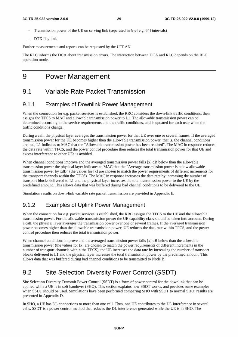
3GPP

3G TR 25.922 V2.0.0 (1999-12)293G TR 25.922 version 2.0.0

- Transmission power of the UE on serving link (separated in NTX [e.g. 64] intervals)

- DTX flag link

Further measurements and reports can be requested by the UTRAN.

The RLC informs the DCA about transmission errors. The interaction between DCA and RLC depends on the RLCoperation mode.

9 Power Management

9.1 Variable Rate Packet Transmission

9.1.1 Examples of Downlink Power Management

When the connection for e.g. packet services is established, the RRC considers the down-link traffic conditions, thenassigns the TFCS to MAC and allowable transmission power to L1. The allowable transmission power can bedetermined according to the service requirements and the traffic conditions, and is updated for each user when thetraffic conditions change.

During a call, the physical layer averages the transmission power for that UE over one or several frames. If the averagedtransmission power for the UE becomes higher than the allowable transmission power, that is, the channel conditionsare bad, L1 indicates to MAC that the "Allowable transmission power has been reached". The MAC in response reducesthe data rate within TFCS, and the power control procedure then reduces the total transmission power for that UE andexcess interference to other UEs is avoided.

When channel conditions improve and the averaged transmission power falls [x] dB below than the allowabletransmission power the physical layer indicates to MAC that the "Average transmission power is below allowabletransmission power by xdB" (the values for [x] are chosen to match the power requirements of different increments forthe transport channels within the TFCS). The MAC in response increases the data rate by increasing the number oftransport blocks delivered to L1 and the physical layer increases the total transmission power to the UE by thepredefined amount. This allows data that was buffered during bad channel conditions to be delivered to the UE.

Simulation results on down-link variable rate packet transmission are provided in Appendix E.

9.1.2 Examples of Uplink Power Management

When the connection for e.g. packet services is established, the RRC assigns the TFCS to the UE and the allowabletransmission power. For the allowable transmission power the UE capability class should be taken into account. Duringa call, the physical layer averages the transmission power over one or several frames. If the averaged transmissionpower becomes higher than the allowable transmission power, UE reduces the data rate within TFCS, and the powercontrol procedure then reduces the total transmission power.

When channel conditions improve and the averaged transmission power falls [x] dB below than the allowabletransmission power (the values for [x] are chosen to match the power requirements of different increments in thenumber of transport channels within the TFCS), the UE increases the data rate by increasing the number of transportblocks delivered to L1 and the physical layer increases the total transmission power by the predefined amount. Thisallows data that was buffered during bad channel conditions to be transmitted to Node B.

9.2 Site Selection Diversity Power Control (SSDT)Site Selection Diversity Transmit Power Control (SSDT) is a form of power control for the downlink that can beapplied while a UE is in soft handover (SHO). This section explains how SSDT works, and provides some exampleswhen SSDT should be used. Simulations have been performed comparing SHO with SSDT to normal SHO: results arepresented in Appendix D.

In SHO, a UE has DL connections to more than one cell. Thus, one UE contributes to the DL interference in severalcells. SSDT is a power control method that reduces the DL interference generated while the UE is in SHO. The

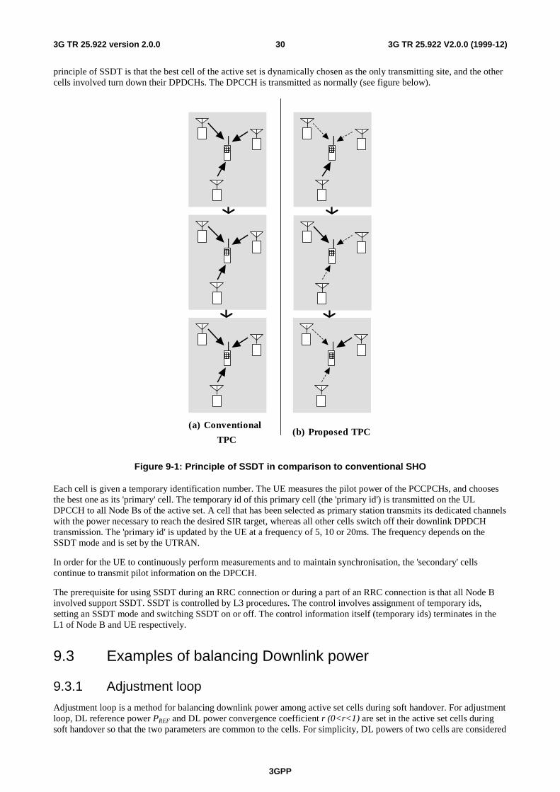
3GPP

3G TR 25.922 V2.0.0 (1999-12)303G TR 25.922 version 2.0.0

principle of SSDT is that the best cell of the active set is dynamically chosen as the only transmitting site, and the othercells involved turn down their DPDCHs. The DPCCH is transmitted as normally (see figure below).

(b) Proposed TPC(a) Conventional

TPC

Figure 9-1: Principle of SSDT in comparison to conventional SHO

Each cell is given a temporary identification number. The UE measures the pilot power of the PCCPCHs, and choosesthe best one as its 'primary' cell. The temporary id of this primary cell (the 'primary id') is transmitted on the ULDPCCH to all Node Bs of the active set. A cell that has been selected as primary station transmits its dedicated channelswith the power necessary to reach the desired SIR target, whereas all other cells switch off their downlink DPDCHtransmission. The 'primary id' is updated by the UE at a frequency of 5, 10 or 20ms. The frequency depends on theSSDT mode and is set by the UTRAN.

In order for the UE to continuously perform measurements and to maintain synchronisation, the 'secondary' cellscontinue to transmit pilot information on the DPCCH.

The prerequisite for using SSDT during an RRC connection or during a part of an RRC connection is that all Node Binvolved support SSDT. SSDT is controlled by L3 procedures. The control involves assignment of temporary ids,setting an SSDT mode and switching SSDT on or off. The control information itself (temporary ids) terminates in theL1 of Node B and UE respectively.

9.3 Examples of balancing Downlink power

9.3.1 Adjustment loop

Adjustment loop is a method for balancing downlink power among active set cells during soft handover. For adjustmentloop, DL reference power PREF and DL power convergence coefficient r (0<r<1) are set in the active set cells duringsoft handover so that the two parameters are common to the cells. For simplicity, DL powers of two cells are considered

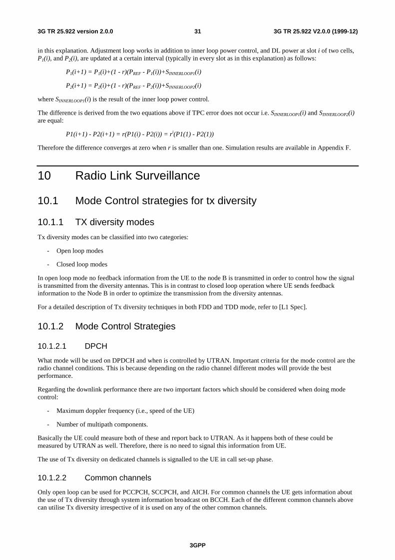
3GPP

3G TR 25.922 V2.0.0 (1999-12)313G TR 25.922 version 2.0.0

in this explanation. Adjustment loop works in addition to inner loop power control, and DL power at slot i of two cells,P1(i), and P2(i), are updated at a certain interval (typically in every slot as in this explanation) as follows:

P1(i+1) = P1(i)+(1 - r)(PREF - P1(i))+SINNERLOOP1(i)

P2(i+1) = P2(i)+(1 - r)(PREF - P2(i))+SINNERLOOP2(i)

where SINNERLOOP1(i) is the result of the inner loop power control.

The difference is derived from the two equations above if TPC error does not occur i.e. SINNERLOOP1(i) and SINNERLOOP2(i)are equal:

P1(i+1) - P2(i+1) = r(P1(i) - P2(i)) = ri(P1(1) - P2(1))

Therefore the difference converges at zero when r is smaller than one. Simulation results are available in Appendix F.

10 Radio Link Surveillance

10.1 Mode Control strategies for tx diversity

10.1.1 TX diversity modes

Tx diversity modes can be classified into two categories:

- Open loop modes

- Closed loop modes

In open loop mode no feedback information from the UE to the node B is transmitted in order to control how the signalis transmitted from the diversity antennas. This is in contrast to closed loop operation where UE sends feedbackinformation to the Node B in order to optimize the transmission from the diversity antennas.

For a detailed description of Tx diversity techniques in both FDD and TDD mode, refer to [L1 Spec].

10.1.2 Mode Control Strategies

10.1.2.1 DPCH

What mode will be used on DPDCH and when is controlled by UTRAN. Important criteria for the mode control are theradio channel conditions. This is because depending on the radio channel different modes will provide the bestperformance.

Regarding the downlink performance there are two important factors which should be considered when doing modecontrol:

- Maximum doppler frequency (i.e., speed of the UE)

- Number of multipath components.

Basically the UE could measure both of these and report back to UTRAN. As it happens both of these could bemeasured by UTRAN as well. Therefore, there is no need to signal this information from UE.

The use of Tx diversity on dedicated channels is signalled to the UE in call set-up phase.

10.1.2.2 Common channels

Only open loop can be used for PCCPCH, SCCPCH, and AICH. For common channels the UE gets information aboutthe use of Tx diversity through system information broadcast on BCCH. Each of the different common channels abovecan utilise Tx diversity irrespective of it is used on any of the other common channels.

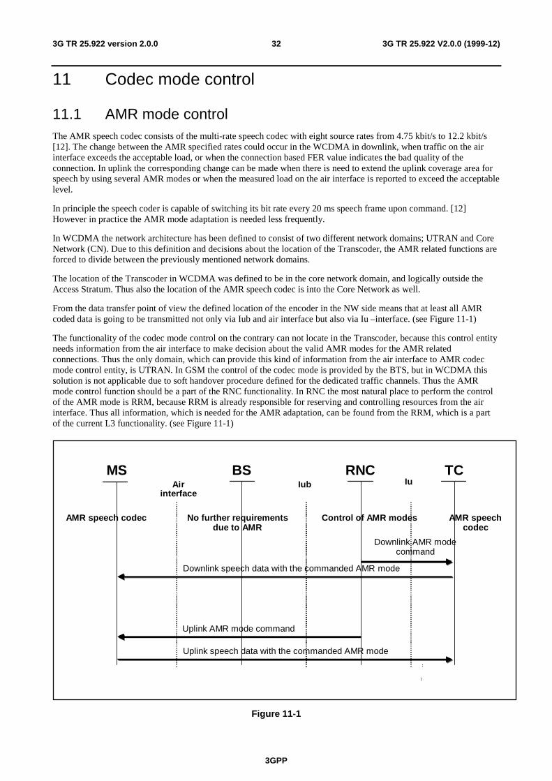
3GPP

3G TR 25.922 V2.0.0 (1999-12)323G TR 25.922 version 2.0.0

11 Codec mode control

11.1 AMR mode controlThe AMR speech codec consists of the multi-rate speech codec with eight source rates from 4.75 kbit/s to 12.2 kbit/s[12]. The change between the AMR specified rates could occur in the WCDMA in downlink, when traffic on the airinterface exceeds the acceptable load, or when the connection based FER value indicates the bad quality of theconnection. In uplink the corresponding change can be made when there is need to extend the uplink coverage area forspeech by using several AMR modes or when the measured load on the air interface is reported to exceed the acceptablelevel.

In principle the speech coder is capable of switching its bit rate every 20 ms speech frame upon command. [12]However in practice the AMR mode adaptation is needed less frequently.

In WCDMA the network architecture has been defined to consist of two different network domains; UTRAN and CoreNetwork (CN). Due to this definition and decisions about the location of the Transcoder, the AMR related functions areforced to divide between the previously mentioned network domains.

The location of the Transcoder in WCDMA was defined to be in the core network domain, and logically outside theAccess Stratum. Thus also the location of the AMR speech codec is into the Core Network as well.

From the data transfer point of view the defined location of the encoder in the NW side means that at least all AMRcoded data is going to be transmitted not only via Iub and air interface but also via Iu –interface. (see Figure 11-1)

The functionality of the codec mode control on the contrary can not locate in the Transcoder, because this control entityneeds information from the air interface to make decision about the valid AMR modes for the AMR relatedconnections. Thus the only domain, which can provide this kind of information from the air interface to AMR codecmode control entity, is UTRAN. In GSM the control of the codec mode is provided by the BTS, but in WCDMA thissolution is not applicable due to soft handover procedure defined for the dedicated traffic channels. Thus the AMRmode control function should be a part of the RNC functionality. In RNC the most natural place to perform the controlof the AMR mode is RRM, because RRM is already responsible for reserving and controlling resources from the airinterface. Thus all information, which is needed for the AMR adaptation, can be found from the RRM, which is a partof the current L3 functionality. (see Figure 11-1)

Airinterface

Iub Iu

Control of AMR modesNo further requirementsdue to AMR

AMR speech codec AMR speechcodec

Uplink AMR mode command

Uplink speech data with the commanded AMR mode

Downlink AMR modecommand

Downlink speech data with the commanded AMR mode

MS BS RNC TC

Figure 11-1

3GPP

3G TR 25.922 V2.0.0 (1999-12)333G TR 25.922 version 2.0.0

In the WCDMA the AMR mode adaptation is carried out with the aid of AMR mode control function, which isresponsible for detecting the need of the AMR mode adaptation and to initiate required procedures to change the currentAMR mode to the newly selected AMR mode. The AMR mode change request can be made with the aid of the AMRmode command, which is sent from the RNC either to the Transcoder for downlink data transfer or to the UE for uplinkdata transfer. In principle the supported AMR mode adaptation can be asymmetric, which implies the possibility to usedifferent AMR modes in uplink and downlink during active speech call.

Therefore, the role of the RRM during the AMR coded speech call will be basically the role of the supervisor of theconnection.

The AMR mode command is used to change the current AMR mode to the new one, which suits better to the conditionson the air interface. The command is sent from the UTRAN to the appropriate AMR codec, which locates either in thetranscoder or in the UE. In which encoder the command is sent depends on direction of the data transmission. If theAMR mode - in question - is intended to be used in downlink the command is sent to the encoder inside the transcodervia Iu –interface, whereas AMR code needed on uplink is sent to the UE through air interface.

The initialization of AMR mode command will base on load information, which has been received from the airinterface. The following table shows the required information during the AMR mode adaptation in WCDMA:

Information used inAMR control

Load

Downlink information BS reports total BS transmissionpower

Uplink information BS measurers total interferencelevel

When RRM indicates the need for the AMR mode adaptation, RRC may generate the requested AMR mode commandand send it to the encoder, or RRC may request MAC –d to perform the same functions. Which layer is used depend onwhether the AMR mode command is intended to use on uplink or on downlink, and whether inband or outbandsignaling is used for transferring the command from the UTRAN to the encoder.

For the downlink, the AMR mode command from RNC to TC is realised as inband.

Transport format for the transport channel carrying the different classes of AMR source codec provides anunambiguous mapping of the codec mode that is used.

3GPP

3G TR 25.922 V2.0.0 (1999-12)343G TR 25.922 version 2.0.0

Appendix A:Simulations on Fast Dynamic Channel Allocation

A.1 Simulation environmentThe presented simulations are performed in the following environments and services according to the requirements inthe following documents:

- ETSI TR 101 112, Selection procedures for the choice of radio transmission technologies of the UniversalMobile Telecommunications System UMTS (UMTS 30.03), version 3.2.0, April 1998.

- Seppo Hämäläinen, Peter Slanina, Magnus Hartman, Antti Lappeteläinen, Harri Holma, Oscar Salonaho, ANovel Interface Between Link and System Level Simulations, Acts Mobile Communications Summit '97, pp.599-604, Aalborg/Denmark, Oct 7-10, 1997.

Absolute capacities [kbit/s/MHz/cell] were published in:

- ETSI Tdoc SMG2 306/98, UTRA TDD Link Level and System Level Simulation Results for ITU Submission,Source: Siemens, Helsinki, Sep 8-11, 1998.

1. Macro (Vehicular) environment for the UDD 144 kbit/s service.

2. Micro (Outdoor-to-Indoor Pedestrian) environment for the UDD 384 kbit/s service.

A.2 ResultsThe relative load of the cell is used for the abscissa (horizontal axis) in all of the plots. Here, a relative load of 100%refers to the maximum cell load obtainable with code-pooling under the ETSI unsatisfied user criterion (in accordancewith ETSI TR 101 112). Vertically, the percentage of unsatisfied users is shown.

A.2.1 Macro UDD 144

In the Macro environment the UDD 144 service is simulated with Hybrid ARQ Type II-III using an adaptive code-ratebetween 1 and ½.

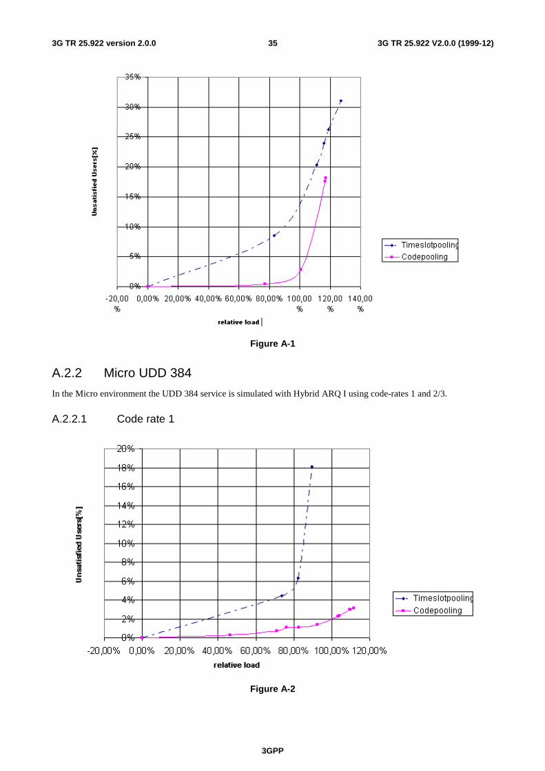
3GPP

3G TR 25.922 V2.0.0 (1999-12)353G TR 25.922 version 2.0.0

Figure A-1

A.2.2 Micro UDD 384

In the Micro environment the UDD 384 service is simulated with Hybrid ARQ I using code-rates 1 and 2/3.

A.2.2.1 Code rate 1

Figure A-2

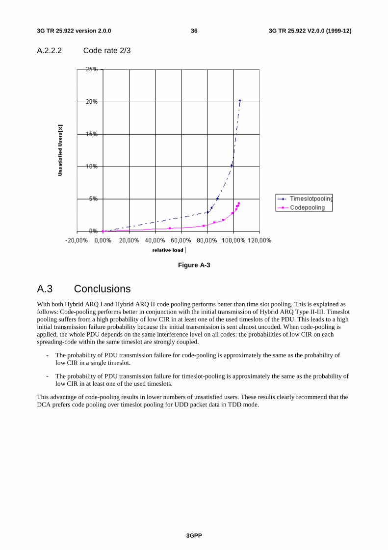
3GPP

3G TR 25.922 V2.0.0 (1999-12)363G TR 25.922 version 2.0.0

A.2.2.2 Code rate 2/3

Figure A-3

A.3 ConclusionsWith both Hybrid ARQ I and Hybrid ARQ II code pooling performs better than time slot pooling. This is explained asfollows: Code-pooling performs better in conjunction with the initial transmission of Hybrid ARQ Type II-III. Timeslotpooling suffers from a high probability of low CIR in at least one of the used timeslots of the PDU. This leads to a highinitial transmission failure probability because the initial transmission is sent almost uncoded. When code-pooling isapplied, the whole PDU depends on the same interference level on all codes: the probabilities of low CIR on eachspreading-code within the same timeslot are strongly coupled.

- The probability of PDU transmission failure for code-pooling is approximately the same as the probability oflow CIR in a single timeslot.

- The probability of PDU transmission failure for timeslot-pooling is approximately the same as the probability oflow CIR in at least one of the used timeslots.

This advantage of code-pooling results in lower numbers of unsatisfied users. These results clearly recommend that theDCA prefers code pooling over timeslot pooling for UDD packet data in TDD mode.

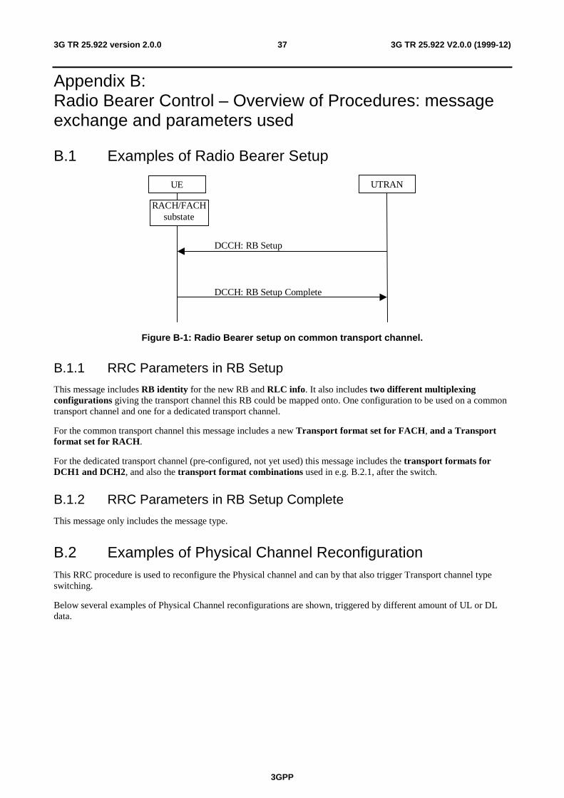
3GPP

3G TR 25.922 V2.0.0 (1999-12)373G TR 25.922 version 2.0.0

Appendix B:Radio Bearer Control – Overview of Procedures: messageexchange and parameters used

B.1 Examples of Radio Bearer Setup

UTRAN

DCCH: RB Setup

DCCH: RB Setup Complete

RACH/FACHsubstate

UE

Figure B-1: Radio Bearer setup on common transport channel.

B.1.1 RRC Parameters in RB Setup

This message includes RB identity for the new RB and RLC info. It also includes two different multiplexingconfigurations giving the transport channel this RB could be mapped onto. One configuration to be used on a commontransport channel and one for a dedicated transport channel.

For the common transport channel this message includes a new Transport format set for FACH, and a Transportformat set for RACH.

For the dedicated transport channel (pre-configured, not yet used) this message includes the transport formats forDCH1 and DCH2, and also the transport format combinations used in e.g. B.2.1, after the switch.

B.1.2 RRC Parameters in RB Setup Complete

This message only includes the message type.

B.2 Examples of Physical Channel ReconfigurationThis RRC procedure is used to reconfigure the Physical channel and can by that also trigger Transport channel typeswitching.

Below several examples of Physical Channel reconfigurations are shown, triggered by different amount of UL or DLdata.

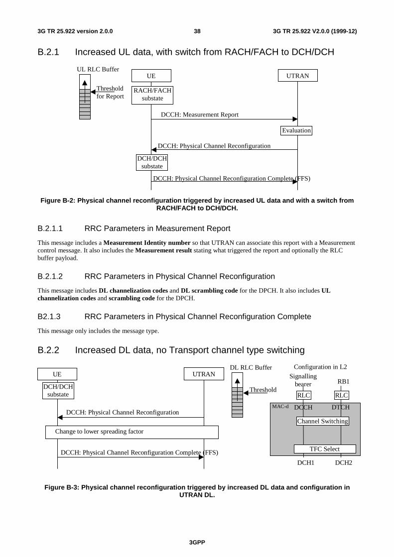
3GPP

3G TR 25.922 V2.0.0 (1999-12)383G TR 25.922 version 2.0.0

B.2.1 Increased UL data, with switch from RACH/FACH to DCH/DCH

UTRAN

DCCH: Physical Channel Reconfiguration

Evaluation

DCCH: Physical Channel Reconfiguration Complete (FFS)

RACH/FACHsubstate

UE

DCH/DCHsubstate

UL RLC Buffer

Thresholdfor Report

DCCH: Measurement Report

Figure B-2: Physical channel reconfiguration triggered by increased UL data and with a switch fromRACH/FACH to DCH/DCH.

B.2.1.1 RRC Parameters in Measurement Report

This message includes a Measurement Identity number so that UTRAN can associate this report with a Measurementcontrol message. It also includes the Measurement result stating what triggered the report and optionally the RLCbuffer payload.

B.2.1.2 RRC Parameters in Physical Channel Reconfiguration

This message includes DL channelization codes and DL scrambling code for the DPCH. It also includes ULchannelization codes and scrambling code for the DPCH.

B2.1.3 RRC Parameters in Physical Channel Reconfiguration Complete


B.2.2 Increased DL data, no Transport channel type switching

MAC-d

UTRAN



DL RLC Buffer

ThresholdDCH/DCHsubstate

Change to lower spreading factor

UEConfiguration in L2

RLC

Signallingbearer

DCH1

RLC

RB1

TFC Select

DCH2

Channel Switching

DCCH DTCH

Figure B-3: Physical channel reconfiguration triggered by increased DL data and configuration inUTRAN DL.

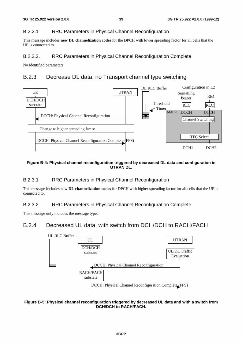
3GPP

3G TR 25.922 V2.0.0 (1999-12)393G TR 25.922 version 2.0.0


This message includes new DL channelization codes for the DPCH with lower spreading factor for all cells that theUE is connected to.

B.2.2.2. RRC Parameters in Physical Channel Reconfiguration Complete

No identified parameters

B.2.3 Decrease DL data, no Transport channel type switching

MAC-d

UTRAN



DL RLC Buffer

Threshold+ Timer

Change to higher spreading factor

UEConfiguration in L2

RLC

DCH1

RLC

TFC Select

DCH2

Channel Switching


DCCH DTCH

DCH/DCHsubstate

Figure B-4: Physical channel reconfiguration triggered by decreased DL data and configuration inUTRAN DL.


This message includes new DL channelization codes for DPCH with higher spreading factor for all cells that the UE isconnected to.

B.2.3.2 RRC Parameters in Physical Channel Reconfiguration Complete


B.2.4 Decreased UL data, with switch from DCH/DCH to RACH/FACH

UTRAN


UL RLC Buffer

UL/DL TrafficEvaluation


RACH/FACHsubstate

UE

DCH/DCHsubstate

Figure B-5: Physical channel reconfiguration triggered by decreased UL data and with a switch fromDCH/DCH to RACH/FACH.

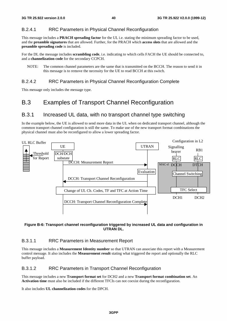
3GPP

3G TR 25.922 V2.0.0 (1999-12)403G TR 25.922 version 2.0.0


This message includes a PRACH spreading factor for the UL i.e. stating the minimum spreading factor to be used,and the preamble signatures that are allowed. Further, for the PRACH which access slots that are allowed and thepreamble spreading code is included.

For the DL the message includes scrambling code, i.e. indicating to which cells FACH the UE should be connected to,and a channelization code for the secondary CCPCH.

NOTE: The common channel parameters are the same that is transmitted on the BCCH. The reason to send it inthis message is to remove the necessity for the UE to read BCCH at this switch.

B.2.4.2 RRC Parameters in Physical Channel Reconfiguration Complete


B.3 Examples of Transport Channel Reconfiguration

B.3.1 Increased UL data, with no transport channel type switching

In the example below, the UE is allowed to send more data in the UL when on dedicated transport channel, although thecommon transport channel configuration is still the same. To make use of the new transport format combinations thephysical channel must also be reconfigured to allow a lower spreading factor.

MAC-d

UTRAN

DCCH: Transport Channel Reconfiguration

DCCH: Transport Channel Reconfiguration Complete

UL RLC Buffer

Thresholdfor Report

DCCH: Measurement Report

Evaluation

Change of UL Ch. Codes, TF and TFC at Action Time

UE

Configuration in L2

RLC

DCH1

RLC

TFC Select

DCH2

Channel Switching


DCCH DTCH

DCH/DCHsubstate

Figure B-6: Transport channel reconfiguration triggered by increased UL data and configuration inUTRAN DL.

B.3.1.1 RRC Parameters in Measurement Report

This message includes a Measurement Identity number so that UTRAN can associate this report with a Measurementcontrol message. It also includes the Measurement result stating what triggered the report and optionally the RLCbuffer payload.

B.3.1.2 RRC Parameters in Transport Channel Reconfiguration

This message includes a new Transport format set for DCH2 and a new Transport format combination set. AnActivation time must also be included if the different TFCIs can not coexist during the reconfiguration.

It also includes UL channelization codes for the DPCH.

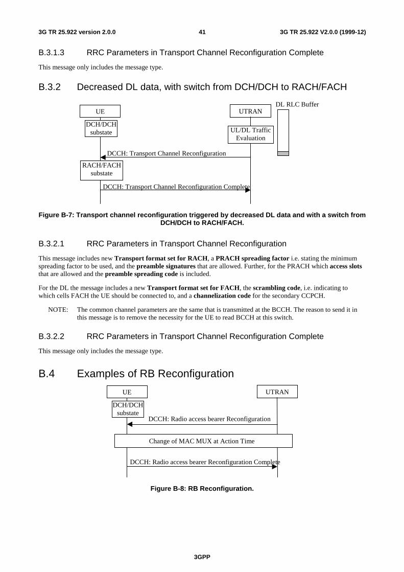
3GPP

3G TR 25.922 V2.0.0 (1999-12)413G TR 25.922 version 2.0.0

B.3.1.3 RRC Parameters in Transport Channel Reconfiguration Complete


B.3.2 Decreased DL data, with switch from DCH/DCH to RACH/FACH

UTRAN

DCCH: Transport Channel Reconfiguration

DL RLC Buffer

UL/DL TrafficEvaluation

DCCH: Transport Channel Reconfiguration Complete

RACH/FACHsubstate

UE

DCH/DCHsubstate

Figure B-7: Transport channel reconfiguration triggered by decreased DL data and with a switch fromDCH/DCH to RACH/FACH.

B.3.2.1 RRC Parameters in Transport Channel Reconfiguration

This message includes new Transport format set for RACH, a PRACH spreading factor i.e. stating the minimumspreading factor to be used, and the preamble signatures that are allowed. Further, for the PRACH which access slotsthat are allowed and the preamble spreading code is included.

For the DL the message includes a new Transport format set for FACH, the scrambling code, i.e. indicating towhich cells FACH the UE should be connected to, and a channelization code for the secondary CCPCH.

NOTE: The common channel parameters are the same that is transmitted at the BCCH. The reason to send it inthis message is to remove the necessity for the UE to read BCCH at this switch.

B.3.2.2 RRC Parameters in Transport Channel Reconfiguration Complete


B.4 Examples of RB Reconfiguration

UTRAN

DCCH: Radio access bearer Reconfiguration

DCCH: Radio access bearer Reconfiguration Complete

UE

Change of MAC MUX at Action Time

DCH/DCHsubstate

Figure B-8: RB Reconfiguration.

3GPP

3G TR 25.922 V2.0.0 (1999-12)423G TR 25.922 version 2.0.0

B.4.1 RRC Parameters in Radio Bearer Reconfiguration

This message includes a multiplexing option with Transport channel identity DCH2 for both RB1 and RB2, stating thatboth these RBs should use the same transport channel. For each of these two RBs a Logical channel identity value anda priority must be given to define the MAC MUX.

Also included is a new Transport format set for DCH2 and a new Transport format combination set (both for ULand DL if the multiplexing is changed both in UL and DL).

It is also possible to reconfigure the physical channel and include new channelization codes for the DPCH withdifferent spreading factor for all cells that the UE is connected to.

B.4.1 RRC Parameters in Radio Bearer Reconfiguration Complete


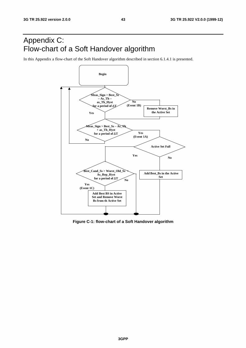
3GPP

3G TR 25.922 V2.0.0 (1999-12)433G TR 25.922 version 2.0.0

Appendix C:Flow-chart of a Soft Handover algorithmIn this Appendix a flow-chart of the Soft Handover algorithm described in section 6.1.4.1 is presented.

Meas_Sign > Best_Ss– As_Th –

as_Th_Hyst for a period of ∆T

Yes

No(Event 1B)

Remove Worst_Bs inthe Active Set

Meas_Sign > Best_Ss – As_Th+ as_Th_Hyst

for a period of ∆T

No

Yes(Event 1A)

Add Best_Bs in the ActiveSet

Best_Cand_Ss > Worst_Old_Ss +As_Rep_Hyst

for a period of ∆T

Yes(Event 1C)

No

Active Set Full

NoYes

Add Best BS in ActiveSet and Remove WorstBs from th Active Set

Begin

Figure C-1: flow-chart of a Soft Handover algorithm

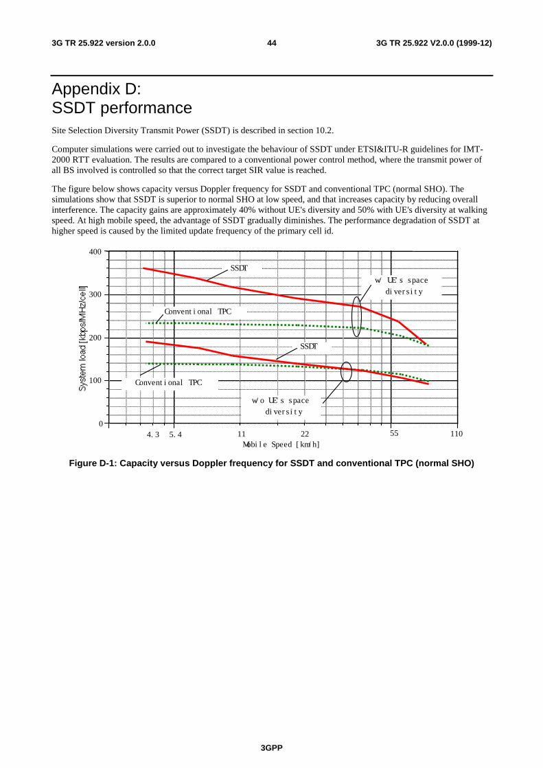
3GPP

3G TR 25.922 V2.0.0 (1999-12)443G TR 25.922 version 2.0.0

Appendix D:SSDT performanceSite Selection Diversity Transmit Power (SSDT) is described in section 10.2.

Computer simulations were carried out to investigate the behaviour of SSDT under ETSI&ITU-R guidelines for IMT-2000 RTT evaluation. The results are compared to a conventional power control method, where the transmit power ofall BS involved is controlled so that the correct target SIR value is reached.

The figure below shows capacity versus Doppler frequency for SSDT and conventional TPC (normal SHO). Thesimulations show that SSDT is superior to normal SHO at low speed, and that increases capacity by reducing overallinterference. The capacity gains are approximately 40% without UE's diversity and 50% with UE's diversity at walkingspeed. At high mobile speed, the advantage of SSDT gradually diminishes. The performance degradation of SSDT athigher speed is caused by the limited update frequency of the primary cell id.

0

100

200

300

400

5. 4 11 110Mobi l e Speed [ km/h]

w/ UE' s spacedi versi ty

w/o UE' s spacedi versi ty

SSDT

SSDT

Conventi onal TPC

Conventi onal TPC

55224. 3

Figure D-1: Capacity versus Doppler frequency for SSDT and conventional TPC (normal SHO)

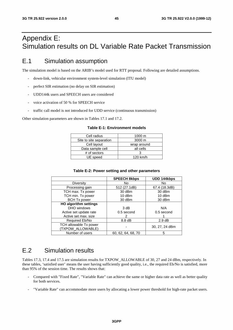
3GPP

3G TR 25.922 V2.0.0 (1999-12)453G TR 25.922 version 2.0.0

Appendix E:Simulation results on DL Variable Rate Packet Transmission

E.1 Simulation assumptionThe simulation model is based on the ARIB’s model used for RTT proposal. Following are detailed assumptions.

- down-link, vehicular environment system-level simulation (ITU model)

- perfect SIR estimation (no delay on SIR estimation)

- UDD144k users and SPEECH users are considered

- voice activation of 50 % for SPEECH service

- traffic call model is not introduced for UDD service (continuous transmission)

Other simulation parameters are shown in Tables 17.1 and 17.2.

Table E-1: Environment models

Cell radius 1000 mSite to site separation 3000 m

Cell layout wrap aroundData sample cell all cells

# of sectors 3UE speed 120 km/h

Table E-2: Power setting and other parameters

SPEECH 8kbps UDD 144kbpsDiversity No No

Processing gain 512 (27.1dB) 67.4 (18.3dB)TCH max. Tx power 30 dBm 30 dBmTCH min. Tx power 10 dBm 10 dBm

BCH Tx power 30 dBm 30 dBmHO algorithm settings

DHO windows 3 dB N/AActive set update rate 0.5 second 0.5 secondActive set max. size 2 1

Required Eb/No 8.8 dB 2.9 dBTCH allowable Tx power(TXPOW_ALLOWABLE) - 30, 27, 24 dBm

Number of users 60, 62, 64, 68, 70 5

E.2 Simulation resultsTables 17.3, 17.4 and 17.5 are simulation results for TXPOW_ALLOWABLE of 30, 27 and 24 dBm, respectively. Inthese tables, ‘satisfied user’ means the user having sufficiently good quality, i.e., the required Eb/No is satisfied, morethan 95% of the session time. The results shows that:

- Compared with "Fixed Rate", "Variable Rate" can achieve the same or higher data rate as well as better qualityfor both services.

- "Variable Rate" can accommodate more users by allocating a lower power threshold for high-rate packet users.

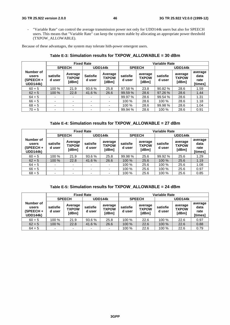
3GPP

3G TR 25.922 V2.0.0 (1999-12)463G TR 25.922 version 2.0.0

- "Variable Rate" can control the average transmission power not only for UDD144k users but also for SPEECHusers. This means that "Variable Rate" can keep the system stable by allocating an appropriate power threshold(TXPOW_ALLOWABLE).

Because of these advantages, the system may tolerate hith-power emergent users.

Table E-3: Simulation results for TXPOW_ALLOWABLE = 30 dBm

Fixed Rate Variable RateSPEECH UDD144k SPEECH UDD144k

Number ofusers

(SPEECH +UDD144k)

satisfied user

AverageTXPOW[dBm]

Satisfied user

AverageTXPOW[dBm]

satisfied user

averageTXPOW[dBm]

satisfied user

averageTXPOW[dBm]

averagedatarate

[times]60 + 5 100 % 21.9 93.6 % 25.8 97.58 % 23.8 90.82 % 28.6 1.5962 + 5 100 % 22.8 41.6 % 26.6 99.59 % 28.6 97.26 % 28.6 1.4464 + 5 - - - - 99.97 % 28.6 99.54 % 28.6 1.3166 + 5 - - - - 100 % 28.6 100 % 28.6 1.1868 + 5 - - - - 100 % 28.6 99.98 % 28.6 1.0470 + 5 - - - - 99.94 % 28.6 100 % 28.6 0.91



Number ofusers

(SPEECH +UDD144k)

satisfied user

AverageTXPOW[dBm]

satisfied user

averageTXPOW[dBm]

satisfied user

averageTXPOW[dBm]

satisfied user

averageTXPOW[dBm]

averagedatarate

[times]60 + 5 100 % 21.9 93.6 % 25.8 99.98 % 25.6 99.92 % 25.6 1.2962 + 5 100 % 22.8 41.6 % 26.6 100 % 25.6 100 % 25.6 1.1964 + 5 - - - - 100 % 25.6 100 % 25.6 1.0866 + 5 - - - - 100 % 25.6 100 % 25.6 0.9768 + 5 - - - - 100 % 25.6 100 % 25.6 0.85



Number ofusers

(SPEECH +UDD144k)

satisfied user

AverageTXPOW[dBm]

satisfied user

averageTXPOW[dBm]

satisfied user

averageTXPOW[dBm]

satisfied user

averageTXPOW[dBm]

averagedatarate

[times]60 + 5 100 % 21.9 93.6 % 25.8 100 % 22.6 100 % 22.6 0.9762 + 5 100 % 22.8 41.6 % 26.6 100 % 22.6 100 % 22.6 0.8864 + 5 - - - - 100 % 22.6 100 % 22.6 0.79

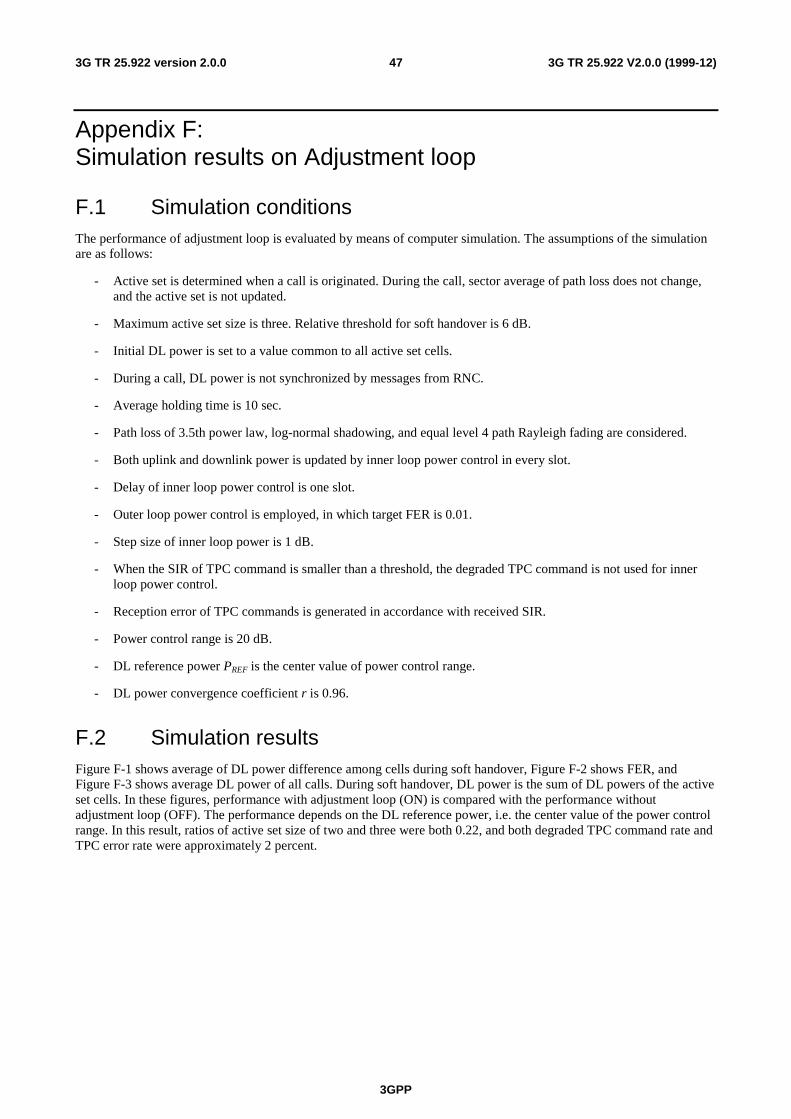
3GPP

3G TR 25.922 V2.0.0 (1999-12)473G TR 25.922 version 2.0.0

Appendix F:Simulation results on Adjustment loop

F.1 Simulation conditionsThe performance of adjustment loop is evaluated by means of computer simulation. The assumptions of the simulationare as follows:

- Active set is determined when a call is originated. During the call, sector average of path loss does not change,and the active set is not updated.

- Maximum active set size is three. Relative threshold for soft handover is 6 dB.

- Initial DL power is set to a value common to all active set cells.

- During a call, DL power is not synchronized by messages from RNC.

- Average holding time is 10 sec.

- Path loss of 3.5th power law, log-normal shadowing, and equal level 4 path Rayleigh fading are considered.

- Both uplink and downlink power is updated by inner loop power control in every slot.

- Delay of inner loop power control is one slot.

- Outer loop power control is employed, in which target FER is 0.01.

- Step size of inner loop power is 1 dB.

- When the SIR of TPC command is smaller than a threshold, the degraded TPC command is not used for innerloop power control.

- Reception error of TPC commands is generated in accordance with received SIR.

- Power control range is 20 dB.

- DL reference power PREF is the center value of power control range.

- DL power convergence coefficient r is 0.96.

F.2 Simulation resultsFigure F-1 shows average of DL power difference among cells during soft handover, Figure F-2 shows FER, andFigure F-3 shows average DL power of all calls. During soft handover, DL power is the sum of DL powers of the activeset cells. In these figures, performance with adjustment loop (ON) is compared with the performance withoutadjustment loop (OFF). The performance depends on the DL reference power, i.e. the center value of the power controlrange. In this result, ratios of active set size of two and three were both 0.22, and both degraded TPC command rate andTPC error rate were approximately 2 percent.

3GPP

3G TR 25.922 V2.0.0 (1999-12)483G TR 25.922 version 2.0.0

0

2

4

6

8

-15 -12 -9 -6 -3 0 3 6 9 12 15

Reference Power [dB]

TX Power Difference

O FF(2BS)

O FF(3BS)

O N(2BS)

O N(3BS)

Figure F-1: DL power difference

0.001

0.01

0.1

-15 -12 -9 -6 -3 0 3 6 9 12 15


Frame Error R

OFF(UL FER)

OFF(DL FER)

ON(UL FER)

ON(DL FER)

Figure F-2: Frame Error Rate

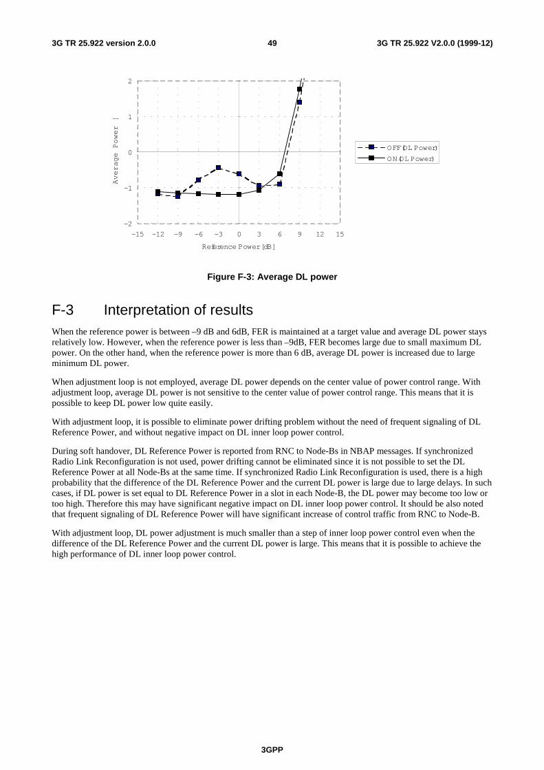
3GPP

3G TR 25.922 V2.0.0 (1999-12)493G TR 25.922 version 2.0.0

-2

-1

0

1

2

-15 -12 -9 -6 -3 0 3 6 9 12 15


Average Power [

OFF(DL Power)

ON(DL Power)

Figure F-3: Average DL power

F-3 Interpretation of resultsWhen the reference power is between –9 dB and 6dB, FER is maintained at a target value and average DL power staysrelatively low. However, when the reference power is less than –9dB, FER becomes large due to small maximum DLpower. On the other hand, when the reference power is more than 6 dB, average DL power is increased due to largeminimum DL power.

When adjustment loop is not employed, average DL power depends on the center value of power control range. Withadjustment loop, average DL power is not sensitive to the center value of power control range. This means that it ispossible to keep DL power low quite easily.

With adjustment loop, it is possible to eliminate power drifting problem without the need of frequent signaling of DLReference Power, and without negative impact on DL inner loop power control.

During soft handover, DL Reference Power is reported from RNC to Node-Bs in NBAP messages. If synchronizedRadio Link Reconfiguration is not used, power drifting cannot be eliminated since it is not possible to set the DLReference Power at all Node-Bs at the same time. If synchronized Radio Link Reconfiguration is used, there is a highprobability that the difference of the DL Reference Power and the current DL power is large due to large delays. In suchcases, if DL power is set equal to DL Reference Power in a slot in each Node-B, the DL power may become too low ortoo high. Therefore this may have significant negative impact on DL inner loop power control. It should be also notedthat frequent signaling of DL Reference Power will have significant increase of control traffic from RNC to Node-B.

With adjustment loop, DL power adjustment is much smaller than a step of inner loop power control even when thedifference of the DL Reference Power and the current DL power is large. This means that it is possible to achieve thehigh performance of DL inner loop power control.

3GPP

3G TR 25.922 V2.0.0 (1999-12)503G TR 25.922 version 2.0.0

Appendix G:Simulation results for CPCHThis appendix presents the results of CPCH simulations performed with the OPNET Modeler tool for various trafficloading and cell capacity scenarios. Simulation assumptions and results are presented. The last section of the appendixpresents RRM strategies based on the simulation results.

G.1 Simulation Assumptions- Results of Link Level Simulations with ITU channel model is used.

- The preamble detection probability as a function of SNR

- Window-based and timer-based ARQ is used. So it was captured end-to-end delays.

- 50-200 mobiles are randomly distributed in the coverage area of one cell.

- The access Preamble ramp-up and the collision resolution steps are simulated.

- Each packet is processed serially and independantly of others, i.e. aggregation of packets in the UE is notsimulated.

- The following tunable parameters exist in the simulations:

- N_Max_Frames: maximum length in frames of individual packet

- Number of ramp-ups max: number of AP power ramp up cycles without APCH response before access isaborted and packet transmission fails.

- Traffic model: includes packet inter-arrival time, session inter-arrival time, # of packets per packet call,number of packet calls per session, Session length, average packet size, etc.

- Three various CPCH channel selection algorithms

- The following traffic model is used in the simulations:

- Average packet size: E-mail application 160, 480, 1000 bytes

- # of packets in a packet call = 15

- Packet call inter-arrival time = 0,120

- # of packet calls within a session =1

- Average inter-packet arrival time = 30, 100, 200 ms

- CPCH channel data rates: 2.048 Msps (512 kbps), 384 ksps (96 kbps), 144 ksps (36 kbps), 64 ksps (16 kbps)

- Session arrival = Poisson

- The following results are captured:

- End-to-End Delay, D(e-e), includes UL retransmissions and DL ACK transmission

- Unacknowledged Mode End-to-End Delay, D(un)

- RLC queuing delay, QD

- Radio Access Delay, AD

- MAC collisions, event count for event in which 2 UE attempt access to same CPCH channel in same slot

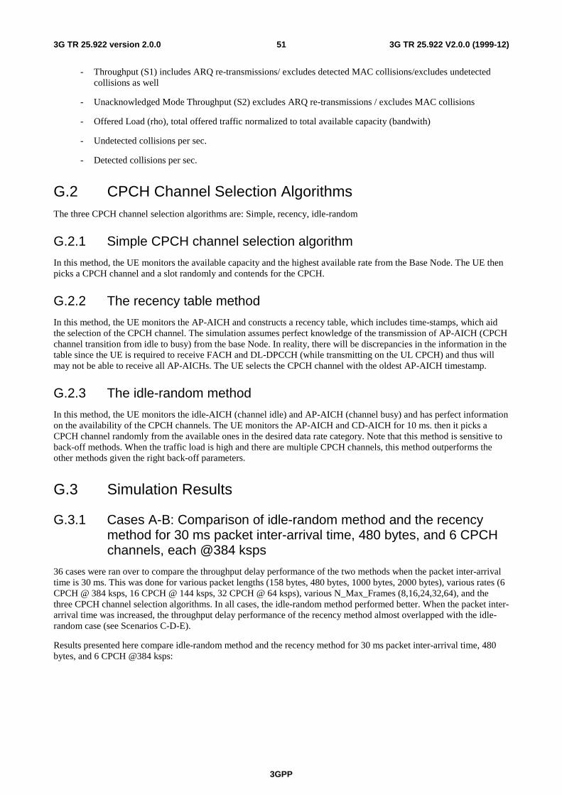
3GPP

3G TR 25.922 V2.0.0 (1999-12)513G TR 25.922 version 2.0.0

- Throughput (S1) includes ARQ re-transmissions/ excludes detected MAC collisions/excludes undetectedcollisions as well

- Unacknowledged Mode Throughput (S2) excludes ARQ re-transmissions / excludes MAC collisions

- Offered Load (rho), total offered traffic normalized to total available capacity (bandwith)

- Undetected collisions per sec.

- Detected collisions per sec.

G.2 CPCH Channel Selection AlgorithmsThe three CPCH channel selection algorithms are: Simple, recency, idle-random

G.2.1 Simple CPCH channel selection algorithm

In this method, the UE monitors the available capacity and the highest available rate from the Base Node. The UE thenpicks a CPCH channel and a slot randomly and contends for the CPCH.

G.2.2 The recency table method

In this method, the UE monitors the AP-AICH and constructs a recency table, which includes time-stamps, which aidthe selection of the CPCH channel. The simulation assumes perfect knowledge of the transmission of AP-AICH (CPCHchannel transition from idle to busy) from the base Node. In reality, there will be discrepancies in the information in thetable since the UE is required to receive FACH and DL-DPCCH (while transmitting on the UL CPCH) and thus willmay not be able to receive all AP-AICHs. The UE selects the CPCH channel with the oldest AP-AICH timestamp.

G.2.3 The idle-random method

In this method, the UE monitors the idle-AICH (channel idle) and AP-AICH (channel busy) and has perfect informationon the availability of the CPCH channels. The UE monitors the AP-AICH and CD-AICH for 10 ms. then it picks aCPCH channel randomly from the available ones in the desired data rate category. Note that this method is sensitive toback-off methods. When the traffic load is high and there are multiple CPCH channels, this method outperforms theother methods given the right back-off parameters.

G.3 Simulation Results

G.3.1 Cases A-B: Comparison of idle-random method and the recencymethod for 30 ms packet inter-arrival time, 480 bytes, and 6 CPCHchannels, each @384 ksps

36 cases were ran over to compare the throughput delay performance of the two methods when the packet inter-arrivaltime is 30 ms. This was done for various packet lengths (158 bytes, 480 bytes, 1000 bytes, 2000 bytes), various rates (6CPCH @ 384 ksps, 16 CPCH @ 144 ksps, 32 CPCH @ 64 ksps), various N_Max_Frames (8,16,24,32,64), and thethree CPCH channel selection algorithms. In all cases, the idle-random method performed better. When the packet inter-arrival time was increased, the throughput delay performance of the recency method almost overlapped with the idle-random case (see Scenarios C-D-E).

Results presented here compare idle-random method and the recency method for 30 ms packet inter-arrival time, 480bytes, and 6 CPCH @384 ksps:

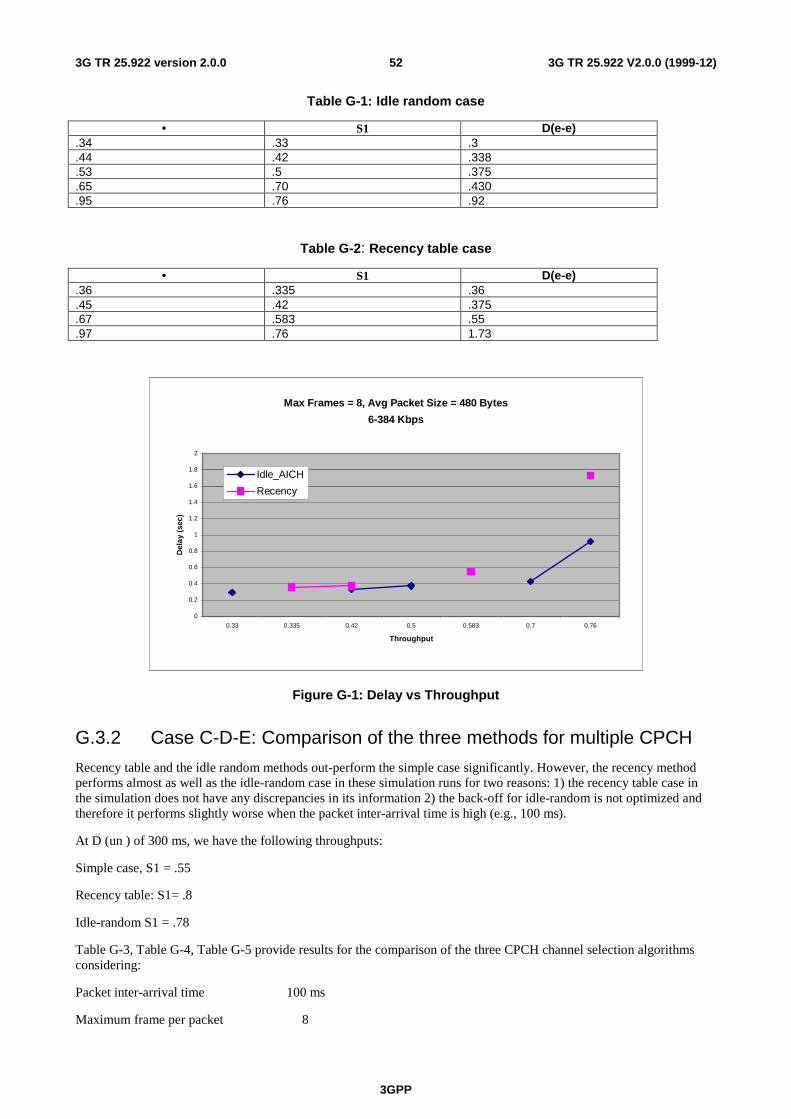
3GPP

3G TR 25.922 V2.0.0 (1999-12)523G TR 25.922 version 2.0.0

Table G-1: Idle random case

• S1 D(e-e).34 .33 .3.44 .42 .338.53 .5 .375.65 .70 .430.95 .76 .92

Table G-2: Recency table case

• S1 D(e-e).36 .335 .36.45 .42 .375.67 .583 .55.97 .76 1.73

Max Frames = 8, Avg Packet Size = 480 Bytes

6-384 Kbps

0

0.2

0.4

0.6

0.8

1

1.2

1.4

1.6

1.8

2

0.33 0.335 0.42 0.5 0.583 0.7 0.76

Throughput

Del

ay (

sec)

Idle_AICH

Recency

Figure G-1: Delay vs Throughput

G.3.2 Case C-D-E: Comparison of the three methods for multiple CPCH

Recency table and the idle random methods out-perform the simple case significantly. However, the recency methodperforms almost as well as the idle-random case in these simulation runs for two reasons: 1) the recency table case inthe simulation does not have any discrepancies in its information 2) the back-off for idle-random is not optimized andtherefore it performs slightly worse when the packet inter-arrival time is high (e.g., 100 ms).

At D (un ) of 300 ms, we have the following throughputs:

Simple case, S1 = .55

Recency table: S1= .8

Idle-random S1 = .78

Table G-3, Table G-4, Table G-5 provide results for the comparison of the three CPCH channel selection algorithmsconsidering:

Packet inter-arrival time 100 ms

Maximum frame per packet 8

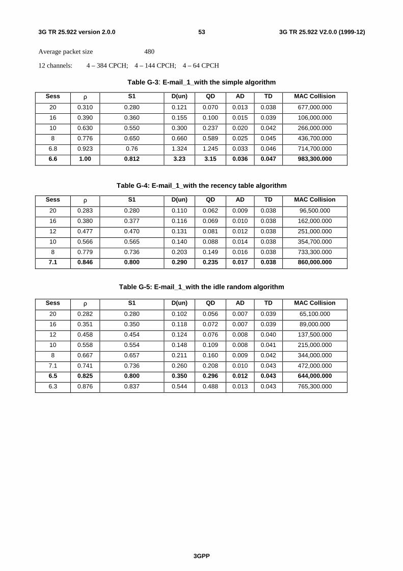
3GPP

3G TR 25.922 V2.0.0 (1999-12)533G TR 25.922 version 2.0.0

Average packet size 480

12 channels: 4 – 384 CPCH; 4 – 144 CPCH; 4 – 64 CPCH

Table G-3: E-mail_1_with the simple algorithm

Sess ρ S1 D(un) QD AD TD MAC Collision

20 0.310 0.280 0.121 0.070 0.013 0.038 677,000.000

16 0.390 0.360 0.155 0.100 0.015 0.039 106,000.000

10 0.630 0.550 0.300 0.237 0.020 0.042 266,000.000

8 0.776 0.650 0.660 0.589 0.025 0.045 436,700.000

6.8 0.923 0.76 1.324 1.245 0.033 0.046 714,700.000

6.6 1.00 0.812 3.23 3.15 0.036 0.047 983,300.000

Table G-4: E-mail_1_with the recency table algorithm


20 0.283 0.280 0.110 0.062 0.009 0.038 96,500.000

16 0.380 0.377 0.116 0.069 0.010 0.038 162,000.000

12 0.477 0.470 0.131 0.081 0.012 0.038 251,000.000

10 0.566 0.565 0.140 0.088 0.014 0.038 354,700.000

8 0.779 0.736 0.203 0.149 0.016 0.038 733,300.000

7.1 0.846 0.800 0.290 0.235 0.017 0.038 860,000.000

Table G-5: E-mail_1_with the idle random algorithm


20 0.282 0.280 0.102 0.056 0.007 0.039 65,100.000

16 0.351 0.350 0.118 0.072 0.007 0.039 89,000.000

12 0.458 0.454 0.124 0.076 0.008 0.040 137,500.000

10 0.558 0.554 0.148 0.109 0.008 0.041 215,000.000

8 0.667 0.657 0.211 0.160 0.009 0.042 344,000.000

7.1 0.741 0.736 0.260 0.208 0.010 0.043 472,000.000

6.5 0.825 0.800 0.350 0.296 0.012 0.043 644,000.000

6.3 0.876 0.837 0.544 0.488 0.013 0.043 765,300.000

3GPP

3G TR 25.922 V2.0.0 (1999-12)543G TR 25.922 version 2.0.0

Max Frames = 8, Avg Packet Size = 480 Bytes4-384 Kbps, 4-144 Kbps, 4-64 Kbps

0

0.5

1

1.5

2

2.5

3

3.5

0.28 0.35 0.36 0.377 0.454 0.47 0.55 0.554 0.565 0.65 0.657 0.736 0.76 0.8 0.812 0.837

Throughput

Del

ay (

sec)

S imple

Recency

Idle_AICH

Figure G-2: Delay vs Throughput

G.3.3 Cases E-F: Impact of packet inter-arrival time

Increasing the packet inter-arrival time from 100 to 200 ms, the throughput delay performance improves significantly.Increasing the packet inter-arrival time, the packet model resembles the Poisson arrival model more. The motivation toincrease the packet inter-arrival time to improve the overall delay performance of all methods. This can be achieved inpractice by having the TFCI and being able to send more packets during a single CPCH transmission if it arrives in theRLC buffer. This is quite possible from a single logical channel. Both Table 19.6 and Table 19.7 provide results for

Idle Random Algorithm

Average packet size 480

16 CPCH channels: 4 – 384 CPCH; 4 – 144 CPCH; 4 – 64 CPCH

Case E (Table G-6) corresponds to packet inter-arrival time of 100 ms presented in the previous section (Table G-5)which is repeated here for convenience. Table G-7 addresses the case of 200 ms packet arrival time.

Table G-6: E-mail_1_with idle random algorithm


20 0.282 0.280 0.102 0.056 0.007 0.039 65,100.000

16 0.351 0.350 0.118 0.072 0.007 0.039 89,000.000

12 0.458 0.454 0.124 0.076 0.008 0.040 137,500.000

10 0.558 0.554 0.148 0.109 0.008 0.041 215,000.000

8 0.667 0.657 0.211 0.160 0.009 0.042 344,000.000

7.1 0.741 0.736 0.260 0.208 0.010 0.043 472,000.000

6.5 0.825 0.800 0.350 0.296 0.012 0.043 644,000.000

6.3 0.876 0.837 0.544 0.488 0.013 0.043 765,300.000

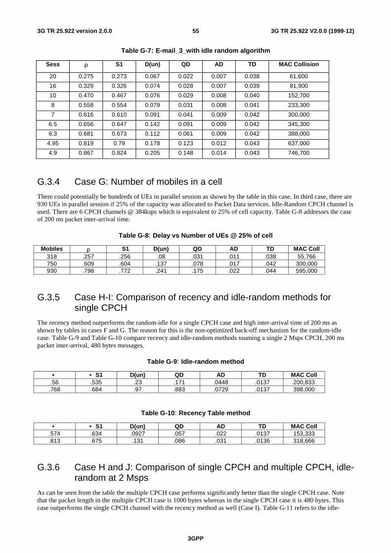
3GPP

3G TR 25.922 V2.0.0 (1999-12)553G TR 25.922 version 2.0.0

Table G-7: E-mail_3_with idle random algorithm


20 0.275 0.273 0.067 0.022 0.007 0.038 61,600

16 0.329 0.326 0.074 0.028 0.007 0.039 81,900

10 0.470 0.467 0.076 0.029 0.008 0.040 152,700

8 0.558 0.554 0.079 0.031 0.008 0.041 233,300

7 0.616 0.610 0.091 0.041 0.009 0.042 300,000

6.5 0.656 0.647 0.142 0.091 0.009 0.042 345,300

6.3 0.681 0.673 0.112 0.061 0.009 0.042 388,000

4.95 0.819 0.79 0.178 0.123 0.012 0.043 637,000

4.9 0.867 0.824 0.205 0.148 0.014 0.043 746,700

G.3.4 Case G: Number of mobiles in a cell

There could potentially be hundreds of UEs in parallel session as shown by the table in this case. In third case, there are930 UEs in parallel session if 25% of the capacity was allocated to Packet Data services. Idle-Random CPCH channel isused. There are 6 CPCH channels @ 384ksps which is equivalent to 25% of cell capacity. Table G-8 addresses the caseof 200 ms packet inter-arrival time.

Table G-8: Delay vs Number of UEs @ 25% of cell

Mobiles ρ S1 D(un) QD AD TD MAC Coll318 .257 .256 .08 .031 .011 .038 55,766750 .609 .604 .137 .078 .017 .042 300,000930 .798 .772 .241 .175 .022 .044 595,000

G.3.5 Case H-I: Comparison of recency and idle-random methods forsingle CPCH

The recency method outperforms the random-idle for a single CPCH case and high inter-arrival time of 200 ms asshown by tables in cases F and G. The reason for this is the non-optimized back-off mechanism for the random-idlecase. Table G-9 and Table G-10 compare recency and idle-random methods ssuming a single 2 Msps CPCH, 200 mspacket inter-arrival, 480 bytes messages.

Table G-9: Idle-random method

• • S1 D(un) QD AD TD MAC Coll.56 .535 .23 .171 .0448 .0137 200,833

.768 .684 .97 .883 .0729 .0137 398,000

Table G-10: Recency Table method

• • S1 D(un) QD AD TD MAC Coll.574 .634 .0927 .057 .022 .0137 153,333.813 .675 .131 .086 .031 .0136 318,666

G.3.6 Case H and J: Comparison of single CPCH and multiple CPCH, idle-random at 2 Msps

As can be seen from the table the multiple CPCH case performs significantly better than the single CPCH case. Notethat the packet length in the multiple CPCH case is 1000 bytes whereas in the single CPCH case it is 480 bytes. Thiscase outperforms the single CPCH channel with the recency method as well (Case I). Table G-11 refers to the idle-

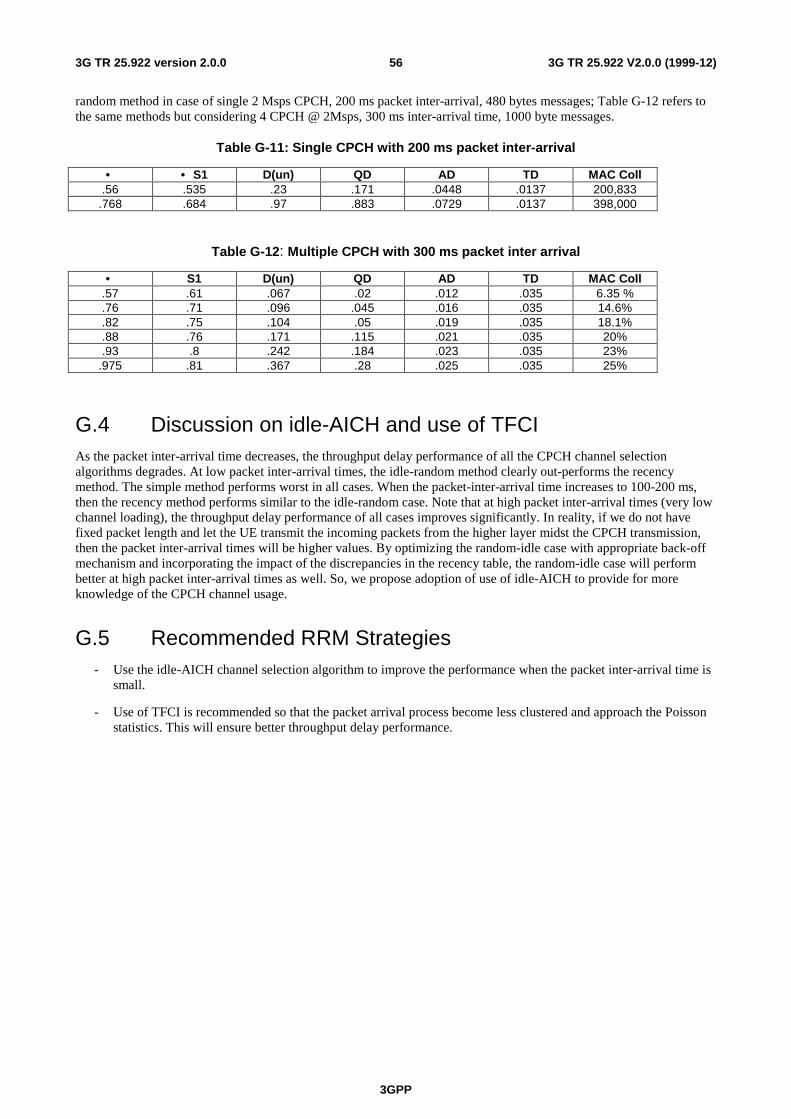
3GPP

3G TR 25.922 V2.0.0 (1999-12)563G TR 25.922 version 2.0.0

random method in case of single 2 Msps CPCH, 200 ms packet inter-arrival, 480 bytes messages; Table G-12 refers tothe same methods but considering 4 CPCH @ 2Msps, 300 ms inter-arrival time, 1000 byte messages.

Table G-11: Single CPCH with 200 ms packet inter-arrival

• • S1 D(un) QD AD TD MAC Coll.56 .535 .23 .171 .0448 .0137 200,833

.768 .684 .97 .883 .0729 .0137 398,000

Table G-12: Multiple CPCH with 300 ms packet inter arrival

• S1 D(un) QD AD TD MAC Coll.57 .61 .067 .02 .012 .035 6.35 %.76 .71 .096 .045 .016 .035 14.6%.82 .75 .104 .05 .019 .035 18.1%.88 .76 .171 .115 .021 .035 20%.93 .8 .242 .184 .023 .035 23%

.975 .81 .367 .28 .025 .035 25%

G.4 Discussion on idle-AICH and use of TFCIAs the packet inter-arrival time decreases, the throughput delay performance of all the CPCH channel selectionalgorithms degrades. At low packet inter-arrival times, the idle-random method clearly out-performs the recencymethod. The simple method performs worst in all cases. When the packet-inter-arrival time increases to 100-200 ms,then the recency method performs similar to the idle-random case. Note that at high packet inter-arrival times (very lowchannel loading), the throughput delay performance of all cases improves significantly. In reality, if we do not havefixed packet length and let the UE transmit the incoming packets from the higher layer midst the CPCH transmission,then the packet inter-arrival times will be higher values. By optimizing the random-idle case with appropriate back-offmechanism and incorporating the impact of the discrepancies in the recency table, the random-idle case will performbetter at high packet inter-arrival times as well. So, we propose adoption of use of idle-AICH to provide for moreknowledge of the CPCH channel usage.

G.5 Recommended RRM Strategies- Use the idle-AICH channel selection algorithm to improve the performance when the packet inter-arrival time is

small.

- Use of TFCI is recommended so that the packet arrival process become less clustered and approach the Poissonstatistics. This will ensure better throughput delay performance.

3GPP

3G TR 25.922 V2.0.0 (1999-12)573G TR 25.922 version 2.0.0

History

Document history

V2.0.0 December 1998 Agreed by TSG-RAN WG2

handover strategies

Documents