COOPERATIVE CONTROL OF PAYLOAD TRANSPORT BY

MOBILE MANIPULATOR COLLECTIVES

by

HAO SU

JUNE 2008

A thesis submitted to the Faculty of the Graduate School of the State University of New York at

Buffalo in partial fulfillment of the requirements for the degree of

MASTER OF SCIENCE

Department of Mechanical and Aerospace Engineering

State University of New York at Buffalo

Buffalo, New York 14260

II

To my family and friends

III

Acknowledgement

I would like to express my gratitude to my advisor, Dr. Venkat Krovi, for all the

guidance and help in my graduate study at the University at Buffalo. He introduced the

fabulous robotics world to me, and articulated many important concepts and ideas in an

insightful and intuitive way. I believe all of these would be invaluable knowledge for my

future career.

I am honored to have Dr. Roger Mayne and Dr. Puneet Singla serving on my

thesis committee. I am also grateful to Dr. Tarunraj Singh and Dr. John Crassidis for

teaching me control theory and Dr. Kemper Lewis for helping me when I first came here.

I would also like to thank all of the ARMLAB members, especially Rajan, Chin

Pei, Leng-feng, Anand, Kun, Qiushi, Pat, Madu, Srikanth and Yao. A special thanks to

Qiushi: as group partner in so many course projects with me, and the time of coding

multi-robot simulator and studying biped locomotion is priceless treasure for me; as lab

member, it is you that talked with me and helped me to solve many problems I met; as

friend, we play Pingpong (in gym or in lab), tennis and billiard at the depressed moments.

For Pat, I have to say you are such a nice guy! You help me and many lab members the

practical problems and share your (yes, I know sometimes it is cooked by Mother Miller)

fantastic food with us. I am greatly grateful for all your friendship, intelligence, and

patience. I thank Chin Pei as a good mentor for teaching and explaining many robotics

theories, and provide many guidance and illumination in many critical times.

Thanks Madu and Srikanth for talking homework and research with me, and telling

me quite a lot of stuff about India. Li Yuan is the Artificial Wikipedia and GPS in our life,

and it is great please to travel with you and talk with you; Xiang Jianping helped me

IV

make many important decisions and save me quite a lot money on laundry; my nice

roommate Ren Bin makes my life happy and rejoicing. Thanks all my friends at Buffalo,

Yang Yan, Liu Li, Chen Tingting, Xu Jingyang, Hao Fang, Xie Wei, Luo Changsong,

Chris, Sai. Thank you Yaan for your never-ending encouragement and talk with me. You

are an unexpected vista of my life in US.

Finally, I must say that my family has been the biggest help of all throughout my life.

Dad, you are a good officer and also good mentor, always help me to find the “optimal

solution”. Mom, you made so many contributions for our family. I would not be where I

am today without you. My little brother, hope you have good luck in the university!

Thank you all!

V

Table of Contents

Acknowledgement................................................. ....................................................... III List of Figures ....................................................... ......................................................VII List of Tables......................................................... ........................................................ X Abstract ................................................................. ....................................................... XI 1 Introduction ....................................................... ......................................................... 1 1.1 Motivation and Application .................................................................................. 1 1.2 Related Works....................................................................................................... 5 1.3 Problem Statement and Our System ................................................................... 11 1.4 Literature Survey ................................................................................................ 12

1.4.1 Cooperative Articulated Mechanical Systems............................................. 12 1.4.2 Cooperative System of Mobile Manipulators .............................................. 13

1.5 Research Issues ................................................................................................... 15 1.6 Thesis Organization ............................................................................................ 18 2 Background......................................................... ....................................................... 20 2.1 The Operational Space Dynamics Formulation.................................................. 20

2.1.1 Manipulator Dynamics with Environment Interaction ................................ 20 2.1.2 Task/Null Space Decoupled Control ........................................................... 22

2.2 Constrained Lagrange Dynamics........................................................................ 24 2.2.1 Multiplier Form............................................................................................ 24 2.2.2 Solution of the Constrained Dynamics Problem.......................................... 26 2.2.3 Energy Minimization Perspective of Dynamic Consistent Matrix .............. 26

3 Force Control of Manipulators ........................... ....................................................... 29 3.1 Impedance Control.............................................................................................. 31 3.2 Hybrid Motion/Force Control ............................................................................. 34 4 Dynamics and Control of Mobile Manipulator Collectives....................................... 38 4.1 Mobile Robot Kinematics and Dynamics ........................................................... 38

4.1.1 Mobile Robot Kinematics ............................................................................ 38 4.1.2 Mobile Robot Dynamics .............................................................................. 43

4.2 Mobile Manipulator Kinematics and Dynamics ................................................. 45 4.2.1 Mobile Manipulator Kinematics .................................................................. 45 4.2.2 Mobile Manipulator Dynamics .................................................................... 48

4.3 Molding of Multi-Grasp Manipulation ............................................................... 51 4.4 Decentralized Control of Mobile Manipulator Collectives ................................ 55 5 Formation Control of Mobile Manipulator Collectives............................................. 59 5.1 Motivation and Review....................................................................................... 59 5.2 Trajectory Tracking and Collision Avoidance of WMR .................................... 59 5.3 Cooperative Collision Avoidance of WMR........................................................ 67 5.4 Formation Control of WMR ............................................................................... 68 6 Simulation Results.............................................. ....................................................... 70 6.1 Cooperative Payload Transport Simulation........................................................ 70

6.1.1 Case Study I: Without Uncertainty.............................................................. 72 6.1.2 Case Study II: With Mass Uncertainty ........................................................ 75

6.2 Formation Control Simulation ............................................................................ 77

VI

6.2.1 Case Study I: Mobile Base Tracking and End-Effector Perform Different Tracking .................................................................................................................... 77 6.2.2 Case Study II: WMMs Formation Control .................................................. 78

7 Force Control Experiment .................................. ....................................................... 80 7.1 ATI Force Sensor Overview ............................................................................... 80

7.1.1 Multiple Calibrations ................................................................................... 80 7.1.2 Multiple Configurations...............................................................................80 7.1.3 Force and Torque Values ............................................................................. 81 7.1.4 Tool Transformations................................................................................... 81 7.1.5 Power Supply............................................................................................... 81

7.2 ATI Force Sensor System Architecture .............................................................. 81 7.2.1 Force/Torque Transducer Working Mechanism.......................................... 81 7.2.2 System Connection ...................................................................................... 82 7.2.3 Hardware Setup............................................................................................ 84

7.3 MATLAB Interface Setup .................................................................................. 85 7.3.1 Communication Protocol ............................................................................. 85 7.3.2 UDP Interface .............................................................................................. 87 7.3.3 MATLAB Program Implementation............................................................ 87

7.4 End-effector Design ............................................................................................ 90 7.5 Force Control Simulation.................................................................................... 93 7.6 Force Sensor and Motor Calibration................................................................... 95 8 Conclusion and Future Work.............................. ....................................................... 98 8.1 Summary............................................................................................................. 98 8.2 Future Work ........................................................................................................ 99 Reference............................................................... ..................................................... 100 Appendix ............................................................... ..................................................... 103 Mechanical Design...................................................................................................... 103

VII

List of Figures

Figure 1: Principal research topics in multi-robot systems [2] ........................................... 2

Figure 2 : Controller archtecture: (a) Centralized control, (b) Decentralized control ........ 3

Figure 3: Engineeing examples of cooperation: (a) EPuck robots, (b) Fleet of marine surface vessels.(c) Italian acrobatic .................................................................................... 4

Figure 4: Three primitive behavior of Boids [3]................................................................. 5

Figure 5: Group behavior of Boids [3] ............................................................................... 6

Figure 6: Group behavior in nature and human society...................................................... 7

Figure 7: Multi-fingered robot and multiple legged robot.................................................. 7

Figure 8: Mobile robot soccer team and Sony AIBO robot soccer team............................ 8

Figure 9: Some mobile manipulator prototypes................................................................ 10

Figure 10: Cooperative mobile manipulators ................................................................... 10

Figure 11: Wheeled mobile manipulator collective with payload: (a) Top view, (b) Side view................................................................................................................................... 12

Figure 12: Wheeled mobile manipulator collective with payload makes an ideal paralel parking manuver ............................................................................................................... 17

Figure 13: Difficulties of payload transport with NH-WMM .......................................... 18

Figure 14: Operational space motion/force control architecture( modified from [26, 27])........................................................................................................................................... 24

Figure 15: Visualization of constrained space [28] .......................................................... 25

Figure 16: One d.o.f impedance control ........................................................................... 30

Figure 17: Impedance control diagram............................................................................. 31

Figure 18: One d.o.f impedance control ........................................................................... 32

Figure 19: A generic structure of hybrid force control [31] ............................................. 34

Figure 20: Original structure of hybrid force control ....................................................... 35

Figure 21: A holonomic mobile robot prototype [34] ...................................................... 39

Figure 22: Nonholonomic mobile robot kinematics ......................................................... 40

Figure 23: Nomenclature of mobile manipulator kinematics and dynamics .................... 46

Figure 24: Payload grasp nomenclature............................................................................ 52

Figure 25: Hierarchical control scheme for a human finger [39] ..................................... 56

Figure 26:Schematic diagram of two cooperative robot modules with a common payload........................................................................................................................................... 57

Figure 27: Decentralized controller of the cooperative payload transport system ........... 58

VIII

Figure 28:The detection region and avoidance region...................................................... 61

Figure 29:The Avoidance function ................................................................................... 62

Figure 30: Some infeasible trajectories............................................................................. 64

Figure 31: Snapshot of mobile robot trajectory tracking.................................................. 66

Figure 32: Snapshot of mobile robot collision avoidance ................................................ 66

Figure 33: Two mobile robot perform collision avoidance .............................................. 67

Figure 34: Notation for formation structure...................................................................... 68

Figure 35: Two robot formation control ........................................................................... 69

Figure 36: SimMechanics model of WMM and payload.................................................. 70

Figure 37: Overall simulation routine implementing decentralized control of the cooperative payload transport system............................................................................... 71

Figure 38: SimMechanics model :(a) a nonholonomic wheel; (b) the simulation architecture in SIMULINK............................................................................................... 72

Figure 39: Payload motion profile. (a) Desired and actual trajectory of payload, (b) tracking error in X and Y. ................................................................................................. 73

Figure 40: The mobile platform tracking a line and end-effector tracking a sinusoid curve. (a) base and end-effector tracking results for robot1, (b) base and end-effector tracking results for robot2, (c) Internal force.................................................................................. 75

Figure 41. Payload motion profile with mass uncertainty. (a) Desired and actual trajectory of payload, (b) tracking error in x and y. .......................................................................... 76

Figure 42. The mobile platform tracking a line and end-effector tracking a sinusoid curve with mass uncertainty. (a) base tracking error for robot1, (b) end-effector tracking error for robot1, (c) Internal force ............................................................................................. 77

Figure 43: (a) WMM performs collision avoidance with end-effector tracking straight line and mobile base tracking straight line; (b) WMM performs collision avoidance with end-effector tracking sinusoid and mobile base tracking straight line ............................. 78

Figure 44: (a) WMMs formation result; (b) control torque of WMM 1; (c) control torque of WMM 2 ........................................................................................................................ 79

Figure 45: ATI F/T sensor ................................................................................................ 82

Figure 46: Net F/T System Components .......................................................................... 83

Figure 47: Net F/T System Block Diagram ...................................................................... 83

Figure 48: Force sensor network connection .................................................................... 84

Figure 49: System setup with PC104................................................................................ 85

Figure 50: F/T system SIMULINK command blocks ...................................................... 89

Figure 51: F/T system data reception and display blocks................................................. 90

Figure 52: View of manipulator arm with force sensor.................................................... 91

IX

Figure 53: Exploded view of force sensor with notation.................................................. 92

Figure 54: WMM with mounted force sensor................................................................... 93

Figure 55: Two link manipulator in contact with vertical wall ........................................ 94

Figure 56: Diagram of xPC Target ................................................................................... 94

Figure 57: Force profile under HIC regulation ................................................................. 95

Figure 58: Force reading with 0-5 weights ....................................................................... 95

Figure 59: Schematic of motor control implementation................................................... 96

Figure 60 : Robot configuration of motor calibration....................................................... 96

Figure 61: (a) Calibration of motor 1; (b)Calibration of motor 2 ..................................... 97

Figure 62: Experiment force data ..................................................................................... 97

X

List of Tables

Table 1: Mobile Manipulator Parameters ......................................................................... 72

Table 2: Net F/T Modes.................................................................................................... 85

Table 3: UDP Port Settings............................................................................................... 88

XI

Abstract

Multi-manipulators based mobile manipulation is an important capability to

extend the domain of robotic applications. The novel feature endowed by the combination

of mobility with manipulation is crucial for a number of applications, ranging from

material handling task to planetary exploration. The benefits include increased workspace,

reconfigurability, improved disturbance rejection capabilities and robustness to failure.

The challenges, however, arise from the compatibility of various holonomic and

nonholonomic constraints and kinematic and dynamic redundancy. Moreover,

cooperative manipulation would lead to significant dynamic coupling and requires

delicate motion coordination. Failure to consider these effects can cause excessive

internal forces and high energy consumption, and even destabilize the system.

To deal with these entailed issues, we present a decentralized dynamic control

algorithm for a robot collective consisting of multiple nonholonomic wheeled mobile

manipulators capable of cooperatively transporting a common payload. The

nonholonomic wheeled mobile manipulator consists of a fully-actuated manipulator arm

mounted on a disk-wheeled mobile base. In this algorithm, the high level controller deals

with motion/force control of the payload, at the same time distributes the motion/force

task into individual agents by grasp description matrix. In each individual agent, the low

level controller decomposes the system dynamics into decoupled task space (end-effector

motions/forces) and a dynamically-consistent null-space (internal motions/forces)

component. The agent level control algorithm facilitates the prioritized operational task

accomplishment with the end-effector impedance-mode controller and secondary

null-space control. The scalability and modularity is guaranteed upon the decentralized

XII

control architecture.

Within the dynamic redundancy resolution framework, a decentralized

coordination and formation control with collision avoidance capability is further studied

for mobile manipulator collectives.

A variety of numerical simulations are performed for multiple mobile manipulator

system carrying a payload (with/without uncertainty) to validate this approach. The

simulations test the capability of internal force regulation by cooperative manipulators.

The end-effector and mobile base to tracking capability is also verified in the simulations.

Multiple mobile manipulator collision avoidance is also studied in simulation.

1

1 Introduction

Object transport and manipulation is perhaps the most important robotic task in

the history of robotics. The electrical and mechanical engineers, by taking advantage of

the reverse engineering, have been trying to learn from the nature. Two decades ago,

biologists observed that coordinated motion of animal groups is an interesting and

suggestive phenomenon in nature. A swarm of bees usually collaboratively waggle dance

to communicate for a new flower bush source. Fish schools maneuver and glide

ingeniously to maximize the overall impetus by delicate formation. Revealing the

benefits and mechanism of these behaviors has been one of the constant research interests

of biologists and sociologists are deliberately emulating the collective behavior of nature

in the design of multiple mobile agents. On the other hand, the hardware devolvement

with the advent of inexpensive, embedded microprocessors has technically enabled the

implementation of these behaviors in real world. Self-contained and computationally low

cost intelligent robot agents are coming out of laboratories to real world applications.

1.1 Motivation and Application

In the daily life, human beings usually take advantage of two hands to manipulate

objects, since single hand manipulation is sometimes incapable or not dexterous enough

for some tasks. While for much heavier objects or complex tasks, accumulation of

individual capability is desirable and crucial for task implementation. By this analogy, we

can see the benefits introduced by cooperation. A couple of different reasons account for

deploying multi-robot systems, however, one of the main motivations is that multi-robot

systems can be used to enhance the system effectiveness. By the constraints of robot

2

actuation capability, cooperative robots are able to accomplish many tasks that are far

beyond of individual robot capability. Ideally, to manipulate any large, heavy payload,

we can incorporate as many as smaller, lighter robot modules so as to fulfill the task. This

modular and flexible structure allows for “divide and conquer” approach to take care of

heavy and complex tasks.

The cooperative robot is also advantageous from the perspective of redundancy

and robustness. Using a team of multiple robots would enhance system robustness with

respect to the single point failure in the sense that we can reconfigure the team and

reassign a new task to each agent. Redundancy is frequently used in the systems that

require high fault tolerance and high successful rate, like mars exploration.

Cooperative robotics first comes into the modern engineering researchers’ mind in

the late 1980s with a special focus on multiple manipulators and multiple mobile robots.

The spectrum of engineering perspective of multi-robot system study is considerably

broad and deep. Interested readers can refer to [1, 2] and reference therein for a detailed

description of research areas in multi-robot systems. Here, we briefly review some

pertained principal research topics.

Figure 1: Principal research topics in multi-robot systems [2]

3

Communication: Communication is of paramount importance for the successful

fulfillment of multi-robot systems and it has been extensively studied ever since the

debut of multi-robot research. Information exchange across the system affects the

interactions among subsystems, and it is possible to categorize the communication

schemes as: centralized and decentralized as shown in Figure 2. In the centralized

implementation, a central controller makes use of all agent states to command the

control signal, while in the decentralized case, each robot module is equipped with

individual controller which can only access its own states and the control signal is

generated locally.

(a) (b) Figure 2 : Controller archtecture: (a) Centralized control, (b) Decentralized control Object transport and manipulation: Manipulation is perhaps the most important task of

robotic system, so the extension of this in multi-robot systems naturally has been one

of the important goals in cooperative robots. There are many pertained issues to be

considered in this process like synchronization of the subsystems, control of the

applied forces and motion planning. Detailed issues would be reviewed in the

subsequent section.

Motion coordination: At this level, the system could be composed of a homogenous or

heterogeneous se of robots of certain characteristics. Research themes in this domain

that have been particularly well studied include multi-robot path planning, traffic

4

control, formation generation, and formation keeping [2]. Most of these issues are

now fairly well understood, although demonstration of these techniques in physical

multi-robot teams (rather than in simulation) has been limited.

The promise of collaborative robotic system has been fulfilled in support of

missions pertaining to national defense, homeland security, and environmental

monitoring. Examples of such cooperation includes mobile robot collectives in Figure 3

(a), manned fleet of marine vessels in Figure 3 (b), manned flight aircrafts in Figure 3

(c) and multiple grounded and aerial vehicles in future battlefield as seen in Figure 3 (d).

It is necessary to note that some of the ideas and control approaches introduced in this

thesis within a robotic paradigm can be applied to these more general multiple robotic

systems, like multiple vehicles.

(a) (b)

(c) (d)

Figure 3: Engineeing examples of cooperation: (a) EPuck robots, (b) Fleet of marine surface vessels.(c) Italian acrobatic

air force unit. (d) Multi vehicles in future battlefield

5

1.2 Related Works

The analogy between manned/unmanned aerial vehicles and a swarm of bees or a

school of fish is perhaps the original biological inspiration for robotics engineers. Natural

behavior also provides some envisioning guidance for robotics paradigm of behavior

based control that can be described by the relationship between the three primitives of

robotics: sense, plan, and act. The first engineering work is motivated by application in

the simulation of computer graphics. In 1986, Reynolds [3] made a computer model for

coordinating animal motion as bird flocks or fish schools. This pioneering work inspired

significant efforts in the study of group behaviors.

(a) (b) (c) Figure 4: Three primitive behavior of Boids [3]

Reynolds observed that with the basic flocking model consists of three simple

steering behaviors separation, alignment and cohesion, these behaviors could describe

how an individual boid maneuvers based on the positions and velocities its nearby

flockmates. Figure 4 illustrates the three basic behaviors separation, alignment and

cohesion. The individual boid has access to its flockmates within a certain small

neighborhood around itself. With these simple behavior and limited perception, a fleet of

these simulated “aircrafts” can maneuver and avoid obstacles as shown in Figure 5.

6

Figure 5: Group behavior of Boids [3] With this inspiration of computer graphics, researchers take advantage of “reverse

engineering” to observe and study the group behavior in nature like the one shown in

Figure 6 (a) where a school of fish glides in the sea to decrease power consumption. Fish

schools maneuver intelligently to minimize group energy consumption by delicate

formation. A group of ants collaboratively make payload transport to achieve the task that

is impossible for individual ant. Similar to the origin of computer graphics simulation for

multiple agents, the graphics rendering for bee swarms are still an interesting and

important work in film industry. More intuitively, the coordination of human group

evacuation in emergent condition is posed to be an imperative problem in optimization

arena. Emergency evacuation of people group is also getting more and more research

attention from the perspective of optimization, like door arrangement, optimal route, and

group allocation. Some of the scenarios mentioned above can be visually seen in Figure

6.

7

(a) (b)

Figure 6: Group behavior in nature and human society

Even though the origin of multi robot comes from the computer graphics simulation

and the inspiration of group behavior in nature, we can also trace the similarity and share

a lot of common interests in the traditional robotic systems.

(a) (b)

Figure 7: Multi-fingered robot and multiple legged robot Multi-finger robotics has been one of the most popular research arenas in robotic

community. Multiple articulated robotic fingers can hold a common payload with shared

payload distribution. In this sense, the dynamics of payload system or to say the grasp

system in multi-finger robots is exactly the same as in the multiple payload transport

system, and most of the research issues in grasp problem, like grasp feasibility, force

closure and grasp force optimization would appear in the multiple mobile manipulation

scenarios. Imagine that each finger is a fixed based (they all have the common basis)

robotic manipulator, the way to control this system in a centralized or decentralized

8

manner is a question to be addressed from the computational perspective.

Another related research area that has been well studied is the multi legged systems.

If each leg can be dissembled from the chassis, it can be considered as a mobile

manipulator with nonholonomic and holonomic constraints on the wheel. The difference

with the multiple mobile manipulator system is that the individual leg is fixed on the

common payload, i.e. the chassis, so it can be considered as a special version of the

mobile manipulator system. From this token, we can conclude that multiple mobile

manipulator system is a more complex, higher mobility system that includes various

issues like kinematic constraints (nonholonomic and holonomic), grasp distribution and

motion planning.

(a) (b)

Figure 8: Mobile robot soccer team and Sony AIBO robot soccer team Because of these difficulties mentioned above, and most of computer scientists cast

research effort on this, it is necessary to note that the inchoate research mainly covers the

multiple agent motion coordination and multiple agent communication, particularly in the

robot soccer team. For example, as show in Figure 8, the researchers from Carnegie

Mellon University and Georgia Institute of Technology first developed 3 vs. 3 agents’

robot soccer team in a field of ×2m 3m without communication and then a new

generation of 4 vs. 4 agents’ robot soccer team in a field of ×5m 9m with full autonomy.

9

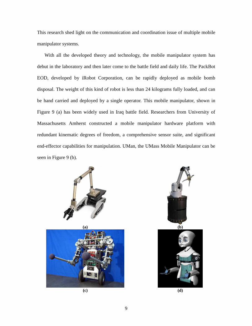
This research shed light on the communication and coordination issue of multiple mobile

manipulator systems.

With all the developed theory and technology, the mobile manipulator system has

debut in the laboratory and then later come to the battle field and daily life. The PackBot

EOD, developed by iRobot Corporation, can be rapidly deployed as mobile bomb

disposal. The weight of this kind of robot is less than 24 kilograms fully loaded, and can

be hand carried and deployed by a single operator. This mobile manipulator, shown in

Figure 9 (a) has been widely used in Iraq battle field. Researchers from University of

Massachusetts Amherst constructed a mobile manipulator hardware platform with

redundant kinematic degrees of freedom, a comprehensive sensor suite, and significant

end-effector capabilities for manipulation. UMan, the UMass Mobile Manipulator can be

seen in Figure 9 (b).

(a) (b)

(c) (d)

10

Figure 9: Some mobile manipulator prototypes The uBot-4, shown in Figure 9 (c), is a two-wheeled dynamically stable bimanual

mobile manipulator. It was designed to combine manipulation and mobility into a small

and cost effective, yet very capable platform. It has been used to study a number of

different robotic manipulation tasks including pushing, pulling, digging, grasping, single

robot transport, and cooperative transport (using multiple copies of the platform).

MIT Media Lab is developing a team of 4 small mobile humanoid robots basing on

the UMass mobile base. The purpose of this platform is to support research and education

goals in human-robot interaction, teaming, and social learning. We can make the analogy

between human and mobile manipulator, in the sense that human feet can be considered

as mobile base and human arm can be considered as mounted manipulator, and human

can be modeled as redundant spatial mobile manipulator to some degree. So it is not

amazing to see that some researchers of mobile manipulators are also focusing on the

study of humanoid robot.

(a) (b)

Figure 10: Cooperative mobile manipulators In parallel with the development of mobile manipulators, some researchers have

begun to take advantage of the cooperative manipulation ability of mobile manipulators.

As seen in Figure 10, a group of research scientists at Stanford University leading by

11

Oussama Khatib have built up spatial wheeled mobile manipulator (for short, we will

note this as WMM) with holonomic motion base. The end-effector of these developed

WMMs has compliant motion capability to work with human in a safety guaranteed

environment. NASA is also a pioneer in WMM development, and two WMMs SRR and

SRR2K acting as the Robot Work Crew can cooperatively transport an extended beam

(2.5 meters long) in a sandy soil terrain with an average slope of 9-degrees. The

cooperative WMMs in this thesis are substantially different from the prior work and

would be detailed below.

1.3 Problem Statement and Our System

Cooperation is one of the key desirable characteristics of next generation robotic

systems. Though much research effort is devoted to this area, less attention is paid to

physically interconnected robotic systems which have many applications that make it of

particular interest for study. Object transport and manipulation by cooperative multi-robot

systems, like multiple planetary rovers [4] and human-supervised multiple mobile robots

[5], is proved to be an effective way to handle complex and heavy payloads in unknown

and dynamic environments.

The goal of our research is to propose a motion/force control law for payload

transport by multiple nonholonomic wheeled mobile manipulators. A decentralized

structure is preferable for scalability and implementation. In the very practical scenario, it

is desirable for the mobile agents to be imposed with avoidance collision capability.

For our system, we consider multiple wheeled mobile robots operating cooperatively

on a common payload. The robots we consider consist of a two-wheel differentially

driven mobile base with a two revolute manipulator mounted on top of the base. Figure

12

11 depicts two of these robots operating on a common payload.

(a) (b) Figure 11: Wheeled mobile manipulator collective with payload: (a) Top view, (b) Side

view.

1.4 Literature Survey

1.4.1 Cooperative Articulated Mechanical Systems

Deploying multiple robots to cooperatively manipulate common payload creates

redundancy, the resolution of which has posed longstanding yet vital challenge to the

robotics community. Examples of cooperative multi-robot systems, ranging from multiple

mobile robots [1], multi-fingered hands [6], and multi-legged vehicles [7] have been

extensively studied in a variety of contexts. Early literature in this field addressed

redundancy resolution in cooperating system from a centralized perspective, i.e., all the

measurements and control signals are generated from a central point.

Under the assumption of perfect knowledge of the system parameters and rigid

grasping of the payload, some control approaches have been proposed. Rigid grasping

means that there is no relative motion between the payload and the manipulator

end-effectors. Arimoto et al. considered the leader-follower scheme in [8] , where one

manipulator acts as a leader controlling the motion of the payload, and other manipulators

act like a followers. The followers’ position is controlled by the motion of the leader in

13

terms of a virtual spring like mechanism to provide certain compliance. Khatib [9]

studied the dynamic properties of redundant manipulators and proposed the augmented

object model for multi-arm cooperation. By considering the parameter uncertainty in the

grasp system, dynamic parameters estimation by least square method is studied in [10]

with an adaptive control law for the motion/force control.

In a later stage, researchers realized the vulnerability of centralized controller which

limits the performance when robot numbers increase. The decentralized version of

leader-follower algorithm is proposed in [11]. Motion/force control of two robots

handling a common payload is implemented therein, and one of the robots is designated

as leader with position control while the other robot is guided as a follower with desired

impedance control. The general multiple manipulation case in [12] presented the

concept of virtual leader, where each individual follower would perceive the rest of the

system as a virtual leader. Later, Liu and Arimoto [13] addressed the adaptive control

problem of multiple redundant manipulators cooperatively handling an object in a

decentralized manner while optimizing a performance index. Szewczyk et al. [14]

presented a distributed impedance approach for multiple robot system control which is

scalable with increased robot modules. More recently, the nominal exponential stability

of collaborative load transport by multiple robots is proved by Montemayor and Wen

[15].

1.4.2 Cooperative System of Mobile Manipulators

Interest has grown in mobile manipulation to achieve cooperative payload

manipulation since the workspace is significantly increased. Again, while the early work

mainly focused on a centralized way, such as Desai et al. [16] studied optimal motion

14

planning for nonholonomic cooperating mobile manipulators grasping and transporting

objects and Tanner et al. [17] presented a motion planning methodology for articulated,

nonholonomic robots with guaranteed collision avoidance. But decentralized approaches

appear to show the greater potential for scalability since a centralized architecture is not

capable of handling increased number of modules. Hirata et al. [18, 19] presented the

extension of their previous 2D case work in [20]. The load is manipulated without

accurately knowing the geometric relationship among the robots when using a virtual 3-D

caster in a leader-follower coordination scheme. This algorithm is basically a

coordination method and controls the position of the followers, and the internal force

regulation is not considered therein. While early efforts deal with holonomic mobile

bases [21, 22], the attention to nonholonomic chained form system permits the ability to

deploy on real world vehicles. In forming such composite systems, it is important to first

ensure capability of various kinematic constraints, both at individual module and system

level. Bhatt et al. [23] established a systematic framework for formulation and evaluation

of system-level performance on the basis of the individual-module characteristics and

affiliated kinematic constraints. A kinematically compatible framework for cooperative

payload transport by nonholonomic mobile manipulators is proposed by Abou-Samah et

al. [24]. Having satisfied kinematic capability, there exits the potential to further optimize

the performances by taking into account of dynamic consideration, such as interaction

forces on actuation level. To facilitate the maintenance of holonomic and nonholonomic

constraints within the system, dynamic controller could achieve better physical

performance and improvement in the actuation input profiles.

15

1.5 Research Issues

While some researchers have attempted to investigate some kinds of mobile

manipulation schemes, in this thesis we will specifically focus on the use of

nonholonomic wheeled mobile manipulators for cooperative payload transport in a

decentralized manner, in addition to this, one pertinent problem is formation control and

obstacle avoidance for multi-agent nonholonomic systems. On this basis, this thesis can

be separated into two parts. In the first part, we will look at how to achieve decentralized

dynamic motion/force control of NH-WMM cooperative manipulation, while the second

part would consider the incorporation of formation control within obstacle avoidance

framework for multiple nonholonomic mobile robot motion planning. Three principal

research questions may be posed and the intimate coupling between these two parts is

illustrated in the posing of these questions.

Research Question 1: What kind of control structure is more suitable for use in

multi-robotic systems?

As noted at the beginning of this section, a decentralized control structure is

usually superior to its centralized counterpart. But how to “divide” the how

complex system into “pieces” and control them individually is not a trivial task.

Research Question 2: How to resolve the various kinematic constraints

(holonomic and nonholonomic) and deal with them in the control algorithm? How to

resolve the multiple levels of redundancies in the modular level which manifests as

dynamic actuation redundancy and in the system level which manifests as grasp force

16

regulation?

The entailed research challenges with respect to this question come from two

aspects. First, the disk-like wheeled mobile bases are subjected to nonholonomic

constraints, and it is well identified by Brockett [25] that nonholonomic systems

as a class of systems that cannot be stabilized via smooth time-invariant state

feedback law. This implies that motion planning and control of such systems

deserves more special treatment. Secondly, the increased workspaces, mobility

and manipulability could be obtained in the cost of considerable redundancy

which needs to be suitably resolved in a dynamic level. With this system structure,

it is worthy to note that three levels of redundancy come into it. First, when given

a starting point and destination point, the nonholonomic motion planning should

be used to solve the indeterminacy. In addition, for individual agent, the mobile

manipulator is kinematically redundant in the sense that the surplus of articulated

degrees of freedoms than the required tasks, and also dynamically redundant

because of the surplus of actuation than the control outputs. The end-effector

motion could be decomposed into displacements of the joints of the manipulator

and rotations of the wheels of the mobile base. Finally, the payload transport is a

planar version of grasp problem, the force distribution and internal force control

should be well resolved in an optimized fashion. After designing a suitable

motion/force controller for the collective, the third research issue immediately

becomes obvious:

17

Figure 12: Wheeled mobile manipulator collective with payload makes an ideal paralel parking manuver

Research Question 3: Which kind of formation control algorithm would be in

accordance with the previous developed decentralized motion/force control law? How to

incorporate obstacle avoidance within all of these control frameworks?

As observed in question 2, for nonholonomic motion planning, even if this

trajectory is a priori specified, it may have to be modified to avoid obstacles as

shown in Figure 12. On a higher level, we notice that the formation control is of a

paramount significance for many engineering and military task. A resolution of

these pertinent problems is indispensable for a diverse array of applications.

All the above mentioned challenges can be seen in Figure 13 where a hierarchical

structure of control problems is illustrated.

18

Dynamic Cooperative Manipulation

RobotModeling

Complexity

Formation Control

Motion Coordination

Internal Force Regulation

Actuation Optimization

Holonomic/Nonholonomic

Constraint

DynamicRedundancy

Leader-follower

Decentralized

Figure 13: Difficulties of payload transport with NH-WMM

1.6 Thesis Organization

The remainder of this thesis is organized as follows:

Chapter 2 provides an overview of a variety of preliminary knowledge on modeling

and control of constrained mechanical systems. Some detailed background theory

includes operational space dynamics and control, constrained Lagrange dynamics.

Since the focus of this thesis is on force control of manipulators, we will introduce

and categorize some popular force control schemes developed since three decades ago in

Chapter 3. We will also highlight the benefits and limitations of some approaches and

show some empirical and visionary perspective basing on the existing experiment results

and some related literature.

Chapter 4 focuses on the modeling and control of WMMs. We begin by investigating

the kinematic and dynamic model of WMR since it’s a sub-system of WMM and many

similar problems of WMMs would be encountered therein, like nonholonomic motion

planning, kinematic and dynamic motion control of nonholonomic systems. Then the

similar analysis would be performed in the WMM system with a focus on task space

19

consistent dynamic control method. As a main body of this thesis, the multiple grasp

modeling would be investigated therein and the decentralized control of WMM

collectives would be presented in this chapter.

To further the theoretical study of WMM control, the formation control of a group of

WMMs would be presented in Chapter 5. The mobile robot formation problem is

investigated first for a basic study, and this problem is split into trajectory tracking and

static obstacle avoidance, formation control and cooperative obstacle avoidance. All of

these results are generalized to mobile manipulator cases.

Chapter 6 presents simulation results for various interesting cases studies using the

dynamic equation formulated in Chapter 3. In particular, the first two case studies were

performed for the dynamic payload transport scenario. The subsequent two cases were

targeted at mobile manipulator collective formation control.

Chapter 7 introduces the experimental setup and verification procedure. This chapter

presented a detailed hardware and software setup basing on the ATI force/torque sensor,

xPC Target and PC/104 platform. A force sensor calibration and manipulator torque

calibration method is proposed therein.

Chapter 8 summarizes the contributions in this work, and concludes with providing

suggestions for future research.

20

2 Background

2.1 The Operational Space Dynamics Formulation

2.1.1 Manipulator Dynamics with Environment Interaction

Before analyzing the dynamic behavior of multiple manipulators, it is necessary to

examine the dynamics of individual module with n degree of freedoms. The dynamics of

an open chain manipulator can be described in the joint space as

τ+ + =ɺɺ ɺ( ) ( , ) ( )M q q C q q G q [2.1]

where ∈ ℝnq is the full set of generalized coordinates, ×∈ ℝ( ) n nM q is the inertia

matrix expressed in terms of the extended coordinate set, ∈ɺ ℝ( , ) nC q q denotes the

Coriolis, centrifugal forces, and ∈ ℝ( ) nG q denotes the gravity force. τ ∈ ℝn is the

generalized control torque.

The forward kinemics of the manipulator with respect to the end-effector position

and orientation, is given by

φ= ( )x q [2.2]

Differentiating the above equation, we can get the mapping between joint space

velocity and end-effector velocity by

=ɺ ɺ( )x J q q [2.3]

where ( )J q is the manipulator’s Jacobian matrix.

When the manipulator end-effector is in contact with the environment, the

constrained dynamic equation of motion would become

τ+ + + =ɺɺ ɺ( ) ( , ) ( ) ( )T

cM q q C q q G q J q F [2.4]

21

where cF is the contact forces at the end-effector.

For redundant manipulators that not in static equilibrium, the mapping from the task

space forces to the joint space forces is surjective. The null space joint torque would not

affect the resulting forces at the end-effector, and the relationship between task space

forces and joint space forces is characterized by

τ τ= + − #0( ) ( ( ) ( ))T T TJ q F I J q J q [2.5]

where I is the ×n n identity matrix, #J is the generalized inverse of J , and τ0 is an

arbitrary generalized joint torques which is projected to the null space of #TJ .

To establish the operational space dynamics, we first use the relationship between

task space acceleration and joint space acceleration = + ɺɺɺ ɺɺ ɺ( ) ( )x J q q J q q , which is

obtained by differentiating =ɺ ɺ( )x J q q . Then we multiply the first equation by the matrix

−1( ) ( )J q M q and use the acceleration relationship

τ

− − −

− −

+ − + + =

+ −

ɺɺɺ ɺ ɺ1 1 1

1 1 #0

( ( ) ( ) ( , ) ( ) ) ( ) ( ) ( ) ( ) ( ) ( )

( ( ) ( ) ( )) ( ) ( )( ( ) ( ))

T

c

T T T

x J q M q C q q J q q J q M q G q J q M q J q F

J q M q J q F J q M q I J q J q

[2.6]

The inverse of the matrix that multipliesF is defined as the task space inertia

matrix − −= 1 1( ) ( ( ) ( ) ( ))TH q J q M q J q . To make the task space acceleration is not affected

byτ0 , we can set the term involving τ0 zero, and this results to

τ− − =1 #0( ) ( )( ( ) ( )) 0T TJ q M q I J q J q [2.7]

22

The joint space inertia weighted generalized inverse of ( )J q , defined

by − − −= 1 1 1( ) ( ) ( )( ( ) ( ) ( ))T TJ q M q J q J q M q J q , and is the unique dynamically consistent

generalized inverse which guarantees the above equation holds.

With this dynamically consistent generalized inverse, it can be shown that the

dynamics of the end-effector can be obtained by projecting the joint space dynamics into

an operational space specified as the end-effector space. This yield

+ + + =ɺɺ ɺ( ) ( , ) ( ) cH q x B q q P q F F [2.8]

where = − ɺɺ ɺ ɺ( , ) ( ) ( , ) ( ) ( )TB q q J q C q q H q J q q and =( ) ( ) ( )TP q J q G q .

2.1.2 Task/Null Space Decoupled Control

Any manipulator dynamic equation described in joint space, like Equation[2.9], can

always be transformed into the operational space, and motion control can be implemented

thereafter basing on the task/null space decoupling. The generalized torque/force

relationship provides the decomposition of the total control torque in Equation [2.10] into

two parts of dynamically decoupled control torque: the one corresponding to the task

behavior and the one that only affects the configuration space behaviors [25, 26]:

τ τ τ= +task config [2.11]

Or the above equation can be explicitly written as

τ τ= + 0( )T TJ q F N [2.12]

where = −( ( ) ( ))T T TN I J q J q .

The dynamically consistent inverse is a generalized inverse that when task space

23

d.o.f is smaller than the configuration space d.o.f., i.e. an underconstrained case. The

dynamically consistent inverse is weighted by the joint space inertia matrix. It is

important to note that the task space force and the null space force are “orthogonal”,

which means that the null space torque would not generated motion in the task space. To

see this point, we calculate (from now on, we would not show the parameter dependence

in the parenthesis for simplicity reason)

τ τ= −0 0( ) ( ) ( )T T T T T TJ F N F J I J J [2.13]

Using the symmetry of− T TI J J , Eqn [2.13] can be rewritten as

τ τ= −0 0( ) ( ) ( )T T T TJ F N F J I JJ [2.14]

Noting that − =( ) 0J I JJ , Eqn [2.14] would show the “orthogonality” between task

space force and the null space force.

The task space control force, can be selected to provide a decoupled control

structure by choosing

= + + +ɶ ɶ ɶ ɶ*cF Hf B P F

where the symbolɶ* denotes the estimation of the quantities. Khatib proposed a

generalized selection matrix as presented in [26]. The force selection matrix is denoted

as Ωf to get the force controlled direction signal, whereas Ωm is used to denote the

motion control direction. The sub-control force is designed as

= Ω +Ω* * *m m f ff f f [2.15]

With appropriate selection matrix, the resulting dynamics would become

=ɺɺ *m mx f [2.16]

=ɺɺ *f fx f [2.17]

24

The motion control input *mf can be designed in terms of the linear system pole

placement method, while the force control input *ff is usually designed based on the

relation between motion and contact forces. The overall control framework is shown in

Figure 14.

Force Control

Task Space Control

Null Space Control

Σ

Σ

Σ

*ff

cF*mf

*ffΩ

mΩ

cF

TN

ˆ ˆB P+

H TJ

τ

df

dx

dV x

Figure 14: Operational space motion/force control architecture( modified from [26, 27])

2.2 Constrained Lagrange Dynamics

2.2.1 Multiplier Form

De Sapio et al. [28] presented an operational space control approach for the general

class of holonomically constrained multibody system. For a more general holonomic

constrained mechanical system, the set of m constraint equations can be written as

φ = 0 [2.18]

The configuration space is constrained on a = −c n m dimensional manifold cQ .

By taking the gradient of the constraint function, we get the constraint matrix

φ∂

=∂

Aq

[2.19]

The constrained dynamic equation can be modified in terms of [2.4] as

25

τ τ+ + = +ɺɺcMq C G [2.20]

where τc is the generalized constrained forces.

ℝ( )TA ℕ( )A

Figure 15: Visualization of constrained space [28] Since the constraints do no virtual work under virtual displacement that is consistent

with the constraint equations, we have τ δ⊥c q for allδ ∈ ℕ( )q A . The symbol ℕ( )A

represents the tangent space of the constraint manifold cQ at some point in the

configuration space ∈ ℝnQ . The generalized constraint forces τc are orthogonal to the

constraint consistent variationsδq . This geometric relation is visualized in Figure 15.

With these derivations, it is easy to see that

τ ⊥∈ =ℕ ℝ( ) ( )T

c A A [2.21]

So the generalized constraint force can be represented as a linear combination of the

columns of TA , i.e.τ λ= T

c A , where λ is an unknown Lagrangian multiplier. Then the

dynamic equation of constrained mechanical system can be expressed in the multiplier

form as

τ λ+ + = +ɺɺ TMq C G A [2.22]

26

2.2.2 Solution of the Constrained Dynamics Problem

To solve the forward dynamics which is usually used in robotic dynamic simulation,

we can assume the Lagrangian multipliers are known, thus the acceleration can be written

as

τ λ−= + − −ɺɺ 1( )Tq M A C G [2.23]

By differentiating the constraint equation twice, we can get

+ =ɺ ɺɺ 0Aq Aq [2.24]

Thus it is easy to find the explicit form of the Lagrangian multipliers as

λ τ− − −= − + + −ɺ ɺ1 1 1( ) ( ( ))TAM A Aq AM C G [2.25]

Following the notation in [29], we can rewrite Equation [2.25] as

λ τ−= − + − −ɺɶ ɺ 1 ( ))uAAq M P C G [2.26]

where − − −=ɶ 1 1 1( )T TA M A AM A and − − −= − 1 1 1( )T T

uP I A AM A AM . The first term

represents the accelerations due to constraint forces− ɺɶ ɺAAq . The projection matrix uP

projects the generalized forces to those that do work on the system, or to say, the forces in

the unconstrained directions. Thus, the joint accelerations come from the contribution of

− ɺɶ ɺAAq and τ− − −1 ( ))uM P C G which are in the constrained and unconstrained

directions respectively.

2.2.3 Energy Minimization Perspective of Dynamic Consistent Matrix

In the first part of this section, we show the derivation dynamically consistent

generalized inverse in the operational space control framework, it is interesting to

perceive this mathematical relation from an emery minimization perspective. Recall that

27

the operational space velocity and joint space velocity is related by the Jacobian matrix as

=ɺ ɺx Jq [2.27]

We would try to find out a solution of Equation [2.27] which minimizes the kinetic

energy of the system

= ɺ ɺ1

2TT q Mq [2.28]

The solution of this constrained optimization problem can be found straightforwardly

as

− − −=ɺ ɺ1 1 1( )T Tq M J JM J x [2.29]

Noting that the dynamically consistent matrix is given by

− − −= 1 1 1( )T TJ M J JM J [2.30]

We have that =ɺ ɺq Jx yields the kinetic energy minimizing the solution of [2.27].

By the same token, we notice that the acceleration relation of operational space

and joint space are related by

= − ɺɺɺ ɺɺ ɺJq x Jq [2.31]

We would like to find the solution which minimize the acceleration energy, defined

as the joint space inertia mass matrix weighted quadratic form

= ɺɺ ɺɺ1

2TE q Mq [2.32]

This solution is obtained as

− − −= − ɺɺɺ ɺɺ ɺ1 1 1( ) ( )T Tq M J JM J x Jq [2.33]

It is just in the form of = − ɺɺɺ ɺɺ ɺ( )q J x Jq that the acceleration energy minimizing

solution of Equation[2.31].

28

29

3 Force Control of Manipulators

Motion control is imperative for a variety of robotic tasks, but for the

accomplishment of more complex robot tasks, motion/force control is more desirable. For

example, one of the most import tasks of mobile robots is localization and mapping, and

belongs to the motion control category. But for mobile manipulator systems, the

capability of manipulation becomes more crucial with the combination of mounted

manipulator and mobile base. With some appropriate control algorithm, it is possible to

decouple the manipulator subsystem apart from the mobile manipulator system, and with

some further modification, it is possible to apply the force control algorithms of general

serial chain manipulators to this new subsystem. To this end, we would take a look at a

diverse array of force control approaches developed since 1980s.

When interaction occurs, the dynamic coupling between the end-effector and the

environment are becoming important. In a motion and force control scenario, interaction

affects the controlled variable, introducing error upon which the controller must act. Even

though it is usually possible to get a reasonably accurate dynamic model of the

manipulator, the main difficulty comes from the dynamic coupling with the environment,

while the later is usually impossible to model or the model is time-varying. A stable

manipulator system could usually destabilized by the environment coupling.

A number of control approaches of robot interaction have been developed in the last

three decades. The robot compliant motion control can be categorized as the one that

performing indirect force control and direct force control. The distinguished difference of

these two approaches is that the former achieve force control via motion control without

explicit force feedback loop, and the later, instead, can regulate the contact force to a

30

desired value because of the explicit force feedback loop.

MasscontrolF enviromentF

x

Figure 16: One d.o.f impedance control

To show the challenge force control, we can see a simple example as shown in Figure

18. One rigid mass object is placed on a horizontal friction plane, and the equation of

motion of the system is

+ = +ɺɺ ɺcontrol enviromentmx bx F F [3.1]

A proportional integral motion controller is applied as

= − + −( ) ( )icontrol p d d

KF K x x x x

s [3.2]

If there is no environmental interaction, that is = 0enviromentF , the closed loop system

would be

+

=+ + +3 2

p i

d p i

K s Kx

x ms bs K s K [3.3]

In terms of the Routh-Hurwitz stability criterion, a condition for the motion control

system is

< p

i

bKK

m [3.4]

But when the robot is in interaction with the enrivoment, or simply coupled to a mass

enviromentm , this condition would become as

31

<+

p

i

enviroment

bKK

m m [3.5]

When the coupled mass is large enough, this condition would not be satisfied,

especially when the environment is a varying system, which is usually not possible for a

constant coefficient controller. So a stable isolated controller does not necessarily work in

contact, even it is just a simple inertia environment.

3.1 Impedance Control

The indirect force control includes compliance (or stiffness) control and impedance

control [30] with the regulation of the relation between position and force (related to the

notion of impedance or admittance). The manipulator under impedance control is

described by an equivalent mass-spring-damper system with the contact force as input.

With the availability of force sensor, the force signal can be used in the control law to

achieve linear and decoupled impedance.

ImpedanceControl

InverseDynamics Robot +Environment

dx

Direct Kinematics

cf

q

Figure 17: Impedance control diagram One simple illustrative example (Mark Spong) of impedance control can be seen in a

one d.o.f system as shown in Figure 18. One rigid mass object is placed on a horizontal

32

frictionless plane, and the equation of motion of the system is

= +ɺɺcontrol enviromentMx F F [3.6]

When the control input is zero, the system is a pure inertia with massM . If the force control is chosen as =control enviromentF mF , the closed loop system is then

= + ⇒ =+

ɺɺ ɺɺ( 1)( 1)

enviroment enviroment

MMx m F x F

m [3.7]

Hence the object now appears to the environment as a modified inertia with

mass+( 1)

M

m. Thus the force feedback has the effect of changing the apparent inertia of

the system.

MasscontrolF

enviromentF

x

Figure 18: One d.o.f impedance control

Impedance control aims at the realization of a suitable relation between the forces and

motion at the point of interaction between the robot and the environment. This relation is

posed as impedance, i.e. describes the velocity as a result of imposed force. The actual

motion and force is then a result of the imposed impedance, reference signals and the

environment admittance (which is the opposite of impedance, i.e. describes the force as a

result of imposed velocity). It is found that impedance control is superior over explicit

force control methods (including hybrid control) in its stability characteristics and

generality, however at the price of accurate force tracking which is better achieved by

explicit force control. It is also shown that some particular formulations of hybrid control

appear as special cases of impedance control, and hence the impedance control method is

selected for further investigation.

33

As mentioned previously, impedance control is based on the recognition of a two way

coupling between manipulator and environment. This coupling may lead to an exchange

of energy between the manipulator and the environment, which has to be managed

properly. In the following a derivation of the impedance control law will be given, and an

attempt to unify impedance control and hybrid control will be given. This will clearly

illustrate that impedance control just as well allows a conceptual separation of

constrained and unconstrained directions, but within one single control law, and without

the stability problems of hybrid control.

The derivation of the standard impedance control law is relatively straightforward, as

it is based on the rigid body equations of the robot

τ+ + + =ɺɺ T

cMq C G J F [3.8]

The goal of impedance control is to transform the robot dynamics by appropriate

selection of the actuator torqueτ , into desired impedance, relating the tip movement to

the external forces.

+ + =ɺɺ ɺeMx Bx Kx F [3.9]

where x is the end-effector coordinates in a suitable coordinate frame (usually in

Cartesian coordinates). The matricesM ,B and K are respectively the target mass,

damping and spring stiffness, which are chosen by the user. Because of simplicity the

target matrices are usually chosen to be constant and diagonal, but the choice is not

limited to this.

Recall the task space and joint space mapping

φ=x [3.10]

=ɺ ɺx Jq [3.11]

34

= + ɺɺɺ ɺɺ ɺx Jq Jq [3.12]

In principle the two equations [3.8] and [3.9] have only one unknown: the actuator

torqueτ , which means that one variable, can be eliminated.

The control law that achieve the target impedance is

τ

− −

= + + +

− − −ɺ ɺ ɺ1 1( )

T

c

c

C G J F

MJ M F MJq BJq Kx [3.13]

The first line of Equation [3.13] eliminates the existing rigid body dynamics, while

the second line inserts the target impedance.

3.2 Hybrid Motion/Force Control

If a detailed model of the environment is available, like the geometry, a widely

adopted strategy is the hybrid motion/force control, which is aimed at explicit position

control in the unconstrained task direction and force control in the constrained task

direction. Usually, a selection matrix is used to filter the direction of position or force that

to be controlled.

Figure 19: A generic structure of hybrid force control [31]

35

Figure 19 illustrates the generic structure for most of the existing hybrid motion/force

control schemes, which are further roughly divided into four categories as shown in [31]:

joint space servoing without inverse dynamics, operational space servoing without

inverse dynamics, operational space servoing with inverse dynamics and constraint space

servoing with inverse dynamics.

. In [32], Raibert and Craig presented the theory, simulation and experiments of

hybrid position force control, and the control diagram can be seen in Figure 20. The most

important characteristic of all hybrid control methods is the complete separation of the

tasks space into two orthogonal subspaces. The constraint surfaces can be quite complex,

such as in case of turning a crank or inserting a screw, or simple as in case of motion

along a plane surface.

The geometric constraint can be expressed by a compliance selection matrix S, which

is generally a diagonal matrix with zeros and ones on the diagonal. A one corresponds to

a position controlled direction, a zero to a force controlled direction. The combination of

position control and force control is then simply an addition of the two controller parts.

S

I-SdF

dx

cF

PositionControl

ForceControl

Robot +Environmentx

Figure 20: Original structure of hybrid force control

τ τ τ= +p f [3.14]

36

where τp and τ f are suitable control torques for position and force control respectively.

In the original formulation by Raibert and Craig, the position control law was chosen to

be a PID type controller:

τ = + +∫ ɺp pp q pi q pd qK e K e dt K e [3.15]

While the force control law was chosen as a saturation type PI controller:

τ τ τ τ= + + ∫ 'f ff fp e fi eK K dt [3.16]

The definition of the variables follows from Figure 20. It is well known that in case of

revolute joints this scheme may suffer from kinematic instability as recognized by An and

Hollerbach [33]. A well known disadvantage of this method is the possibility of the

possibility of kinematic instability, and several remedies have been proposed. Due to the

separation into a position controlled loop and force controlled loop the same control laws

as in case of respectively pure position control and explicit force control method can be

applied.

Another formulation of hybrid position-force control is the operational space

formulation by Khatib as showed in Chapter 2. Now that hybrid motion/force control has

been presented, the explicit control of force should be considered.

=ɺɺ *f fx f [3.17]

The main difficulty of the force control is because of the explicit force control loop. A

significant amount of literature is targeted at resolving this problem, but it is still not fully

addressed. Many proposed explicit force controllers are modified versions of the PID

control law. The most commonly applied method is damped proportional force control

with force feed-forward:

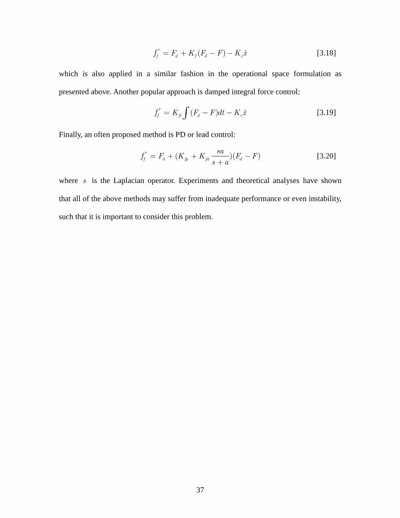
37

= + − − ɺ* ( )f d f d vf F K F F K x [3.18]

which is also applied in a similar fashion in the operational space formulation as

presented above. Another popular approach is damped integral force control:

= − −∫ ɺ* ( )f fi d vf K F F dt K x [3.19]

Finally, an often proposed method is PD or lead control:

= + + −+

* ( )( )f d fp fd d

saf F K K F F

s a [3.20]

where s is the Laplacian operator. Experiments and theoretical analyses have shown

that all of the above methods may suffer from inadequate performance or even instability,

such that it is important to consider this problem.

38

4 Dynamics and Control of Mobile Manipulator Collectives

4.1 Mobile Robot Kinematics and Dynamics

4.1.1 Mobile Robot Kinematics

Wheeled mobile robot (WMR) can be categorized into two basic types as holonomic

and nonholonomic mechanical systems in terms of the kinematic constraints.

Holonomic constraints on the configuration-space of the system can be expressed in

terms of algebraic equations which can be written in the form of:

Φ =( ) 0q [4.1]

where q is the vector of generalized coordinates that describes the configuration of the

system. Nonholonomic constraint is the one that cannot be expressed with purely

configuration variables in the form of

Φ =ɺ( , ) 0q q [4.2]

Mechanical systems that contain nonholonomic constraints can be reformulated in the

Pfaffian form:

( ) =ɺ 0A q q [4.3]

where A is the constraint matrix and is a function of only q . For example a rolling

wheel possesses a holonomic constraint in the rolling direction and a non-holonomic

constraint perpendicular to this.

Specifically, no motion velocity restriction is imposed on holonomic WMR, and

holonomic WMR possesses maximal number of degree of freedoms (as in the planar, it is

39

3). A diverse variety of mechanisms are employed as universal wheels, omni-directional

wheels, orthogonal or ball wheels to implement a holonomic motion. The distinct feature

of holonomic WMR is that it permits easier motion planning comparing with their

nonholonomic counterparts. Figure 21 shows a powered caster version of holonomic

WMR.

Figure 21: A holonomic mobile robot prototype [34]

Nonholonomic WMRs possess less than 3 degree of freedoms (d.o.f). They are simpler

in construction and thus cheaper with less controllable axes and ensure the necessary

mobility in plane. Over the millennia, the “wheeled platform design” with multiple sets

of disc wheels attached to a common chassis has stayed popular for many reasons. Most

importantly, the disk-wheel based design allows for sturdy and robust design

implementation. While the mobility, steerability, and controllability of the overall

wheeled system depend largely upon the type, nature and locations of the attached wheels,

this is a reasonably well understood. See [35, 36] for a survey of some of the different

design configurations possible for wheeled bases, for operation on planar terrain.

In this section, we develop the kinematic model and the terminology for the WMR and

40

the WMM that will be used in subsequent dynamic analysis. First, we consider the

WMR alone and its nonholonomic constraints. Then we consider the addition of the

manipulator and develop all necessary kinematic relationships. Finally, we assemble the

constraint matrix, the nullspace matrix, and construct a Jacobian matrix which relates the

task-space to the joint space.

The WMR in our research is composed of three distinct rigid bodies: mobile base, left

and right wheels. A body fixed frame M attached at the center of mass of the WMR

determines the pose with respect to the fixed ground frame F . The mobile base is

actuated by two independently driven wheels of radii r located at an equal distance b

on either side of the midline. The wheel axes are collinear and are located at a

perpendicular distance ≥ 0d from the center of mass. The instantaneous WMR

configuration can be fully described by the extended set of generalized coordinates:

φ θ θ = c c R Laq x y

lθ

rθ

M

FY

FFX

φ

b

b

1τ

daL

Figure 22: Nonholonomic mobile robot kinematics

41

where ( ),c cx y is the Cartesian coordinates of the center of mass, and φ is the

orientation of the WMR, θR and θL are the angular positions of the left and right

wheels, respectively. For later reference, we note here that the first revolute joint is

located at the look-ahead point which is located at a perpendicular distanceaL .

At the velocity level, the kinematics of the mobile robot can be simply expressed as:

φ

φ

φ ω

=

=

=

ɺ

ɺ

ɺ

cos

sin

x v

y v [4.4]

where ( ),x y is the Cartesian position of the center of the axle of the robot, φ is the

orientation of the robot, v and ω are the linear and angular velocities of the robot. In a

kinematic control scheme, the linear and angular velocities are used as the input to the

system. With the kinematic relation of the mobile platform, the mapping from the wheel

angular velocity to the mobile base linear and angular velocities is

θ

ω θ

= −

ɺ

ɺ

2 2

2 2

R

L

r rv

r r

b b

[4.5]

Similarly, we can find the reverse relation of the two vectors as:

θ

ωθ

= −

ɺ

ɺ

1

1

R

L

bv

r r

b

r r

[4.6]

The system is subjected to 3 nonholonomic constraints. The first constraint of the

mobile base comes from the nonholonomic behavior of the wheels and restricts the

velocity of the WMR in the lateral directions to be zero as

42

φ φ φ− + − =ɺɺ ɺsin cos 0c cx y d [4.7]

The other two constraints, relating the base velocities and the wheel velocities, ensure

the no-slip condition at each rolling wheel in the forward directions.

φ φ φ θ+ + =ɺ ɺɺ ɺcos sinc c Rx y b r [4.8]

φ φ φ θ+ − =ɺ ɺɺ ɺcos sinc c Lx y b r [4.9]

The set of m (=3) constraints can be written in Pfaffian form as:

=ɺ( ) 0 a a aA q q and

φ φ

φ φ

φ φ

− −

= − − − − −

0 0

( ) 0

0

a a

S C d

A q C S b r

C S b r

[4.10]

where φ φ= sinS and φ φ= cosC . By taking the independent joint velocities

of θ θ = ɺ ɺɺ

T

a R Lz , the corresponding null-space matrix that annihilates the constraint

matrix can be determined as:

=ɺ ɺa a aq S z and

( ) ( )( ) ( )

φ φ φ φ

φ φ φ φ

− + + − = −

1 0

0 1

a

c bC dS c bC dS

c bS dC c bS dC

S c c [4.11]

where =2

rc

b. We define a look-ahead point aP with Cartesian coordinates

of ( )= ,a a ax x y , and

φ

φ

= +

= +

a c a

a c a

x x LC

y y L S [4.12]

43

where aL is the distance from the center of mass to aP . The corresponding Jacobian

that relates independent joint velocities to velocity of the look-ahead point can be

determined as:

= = Φɺ ɺ ɺa a a a ax J S z z and

φ

φ

− =

1 0 sin 0 0

0 1 cos 0 0

a

a

a

LJ

L [4.13]

where = +d aL d L . aJ relates the base velocities ɺax to the generalized base velocities

ɺaq .

4.1.2 Mobile Robot Dynamics

The dynamics of a mechanical system can be modeled using a variety of different

techniques. For this thesis we will use the energy-based Lagrange method because of its

simplicity, as outlined by Angeles [37]. Like other energy-based methods, the Lagrange

method only considers external forces acting on the system and neglects all internal

forces. Therefore, the resulting equations of motion are greatly simplified and internal

forces are already factored out.

The energy-based Lagrange method is based on the principle of virtual work. By

accounting for all sources of power entering the system, present in the system, and

leaving the system, the equations of motion can be found. Because joint forces internal

to the system have no accompanying displacements, they do no work and are therefore

not included in the final equations of motion. Angeles [37] has outlined the following

systematic method for finding the unconstrained equations of motion.

1. Introduce a set of generalized coordinates [ ]= 1,....,T

nq q q and their time rates

of change [ ]=ɺ ɺ ɺ1,....,

T

nq q q , defining the state of the system.

44

2. Evaluate = ɺ( , )T T q q , the kinetic energy of the whole system, as the sum of the

individual kinetic-energy expressions.

3. Evaluate = ( )V V q , the potential energy of the whole system, as the sum of the

individual expression, for every element storing potential energy.

4. Evaluate ≡ −L T V , the Lagrangian of the whole system: = ɺ( , )L L q q .

5. Evaluate Π = Π ɺ( , )q q , the power supplied to the system from external sources

Π ≥( 0) . Evaluate its partial derivative ∂Π ∂ ɺ/ q .

6. Evaluate ∆ = ∆ ɺ( , )q q , the sum of the dissipation functions of all dissipative elements of

the system ∆ ≥( 0) , as well as its partial derivative ∂∆ ∂ ɺ/ q .

7. Write the governing equation using the foregoing partial derivatives: ∂ ∂ ∂Π ∂∆ − = − ∂ ∂ ∂ ∂ ɺ ɺ ɺ

d L L

dt q q q q

The resulting equations of motion can then be put in the following matrix form:

τ+ =ɺɺ ɺ( ) ( , )M q q V q q E [4.14]

where M is the mass matrix and contains the inertia terms, τ is the input vector, E

maps the input, τ , to joint-space, and V contains all other position and velocity terms.

Constraints can then be added very easily to the unconstrained dynamics to further

describe the behavior of the system. These could include any combination of holonomic

or nonholonomic constraints. We also note that constraints are the only way to

incorporate nonholonomic behavior into the equations of motion. In either case, the

constraints will be incorporated on the velocity level in the following standard form:

( ) =ɺ 0A q q [4.15]

The constraint forces can then be added to the unconstrained equation of motion[4.14],

by

45

τ λ+ = −ɺɺ ɺ( ) ( , ) TM q q V q q E A [4.16]

where λ is the constraint force and TA maps the constraint force to joint-space.

Specifically, with the help of the null-space matrix, the constrained dynamics of the

WMR can be determined as:

( ) ( ) ( )τ λ+ = −ɺ ɺ, T

aa a a a aa a a a a aM q q c q q E q A [4.17]

where a

q are the generalized coordinates of the mobile base. aM is the configuration

dependent inertial matrix, ac includes all the Coriolis/centrifugal/damping term, and

aE is the actuation transformation matrix that maps the joint torques to the

corresponding independent joint coordinates. λa is the Lagrange multiplier

corresponding to the constraints.

4.2 Mobile Manipulator Kinematics and Dynamics

4.2.1 Mobile Manipulator Kinematics

Kinematic analysis, including forward kinematic and inverse kinematics, is the

essential basis for dynamitic analysis and control. Particularly, the wheeled locomotion

systems possess the nonholonomic characteristics which make the kinematic relation

deserving precautious focus and treatment. From the mechanical perspective, a

manipulator can be schematically represented as an open kinematic chain of rigid bodies

connected by means of (generally revolute or prismatic) joints. The kinematics of a robot

manipulator describes the relationship between the motion of the joints of the

manipulator and the resulting motion of the rigid bodies which from the robot. Moreover,

wheeled systems, because of the rolling contact between the wheel and ground, are

subject to nonholonomic constraints. These constraints can be represented at velocity

46

level and thus becomes an essential element of kinematic analysis of a WMM of the type

shown in Figure 22.

1L1cL

2cL2L

lθ

rθ

2θ

M

1θ

FY

FFX

φ

b

b

1τ

2τ

xF

yF

daL

Figure 23: Nomenclature of mobile manipulator kinematics and

dynamics The full configuration of the base of WMM at any time can be fully described by five

generalized coordinates. These are the three variables that describe the position and

orientation of the platform and two variables that specify the angular positions for the

driving wheels.

φ θ θ = c c R Laq x y [4.18]

The full configuration vector of the WMM can thus by given by augmenting the base

configuration vector with the angles θ1 andθ2 .

47

φ θ θ θ θ = 1 2c c R Lq x y [4.19]

The detailed derivation of homogeneous transform matrices are referred to the

Appendix. Briefly, in terms of the successive homogeneous transform matrices, the

position vectors 1cr and 2cr are given as

= + + + + 1 0 1 01 0 1 01

T

c c a c c a cr x L c L c y L s L s [4.20]

= + + + + + + 2 0 1 01 2 012 0 1 01 2 012

T

c c a c c a cr x L c L c L c y L s L s L s [4.21]

The position vector of the end-effector er is given as

= + + + + + + 0 1 01 2 012 0 1 01 2 012

T

e xb a yb ar r L c L c L c r L s L s L s [4.22]

One can now determine the velocity forward kinematics for each of the different

points of interest (for which we developed the position forward kinematics) using the

twist-based mathematics. We show the process for one case of the location of joint 1 on

the base and present the results for the rest of the cases.

We determine the body fixed twist of the frame using body fixed twist matrix and then

extract the twist vector. The velocity of joint 1 expressed in the inertial frame is given as

φ φ = − + ɺ ɺɺ ɺ

10 0 0

T

c a c av x L s y L c [4.23]

Following a similar procedure, we can determine the expressions for velocities of any

point of interest. The resulting expressions are given below as

φ θ

φ θ

− + − = + + +

ɺ ɺɺ

ɺ ɺɺ1

0 1 01 1 01 1

0

0 1 01 1 01 1

( )

( )c

c a c c

c a c c

x L s L s L sv

y L c L c L c [4.24]

48

( )

φ θ θ

φ θ θ

− + + − + − = + + + + + +

ɺ ɺ ɺɺ

ɺ ɺ ɺɺ2

0 1 01 2 012 1 01 2 012 1 2 012 2

0

0 1 01 2 012 1 01 2 012 1 2 012 2

( ) ( )

( )c

c a c c c

c a c c c

x L s L s L s L s L s L sv

y L c L c L c Lc L c L c [4.25]

( )

φ θ θ

φ θ θ

− + + − + − = + + + + + +

ɺ ɺ ɺɺ

ɺ ɺ ɺɺ

0 1 01 2 012 1 01 2 012 1 2 012 2

0

0 1 01 2 012 1 01 2 012 1 2 012 2

( ) ( )

( )e

c a

c a

x L s L s L s L s L s L sv

y L c L c L c Lc L c L c [4.26]

4.2.2 Mobile Manipulator Dynamics

For the mobile manipulator system, the constraints is of the same as the mobile robot

where the set of constraints can be written in Pfaffian form in terms of the configuration

space of the mobile manipulator as

( ) =ɺ 0A q q [4.27]

where

φ φ

φ φ

φ φ

− −

= − − − − −

sin cos 0 0 0 0

( ) cos sin 0 0 0

cos sin 0 0 0

d

A q b r

b r

.

Considering the nonholonomic constraints, we can now find an appropriate annihilator

matrix that satisfies = 0AS . The set of feasible velocities could be parameterized in

terms of a suitable vector of −n m independent velocities, θ θ θ θ = ɺ ɺ ɺ ɺɺ

1 2

T

r lz as

=ɺ ɺq Sz [4.28]

where =2

rc

b and

( ) ( )

( ) ( )

φ φ φ φ

φ φ φ φ

− + + − − =

cos sin cos sin 0 0

sin cos sin cos 0 0

0 0

1 0 0 0

0 1 0 0

0 0 1 0

0 0 0 1

c b d c b d

c b d c b d

c c

S .

49

If the task space is specified byxy position of the end-effector, the Jacobian that relates

the extended joint-rates,ɺq to the task-space velocityɺx , as:

=ɺ ɺqx J q [4.29]

where φ θ θ

φ θ θ

− − − =

1 1 2 2

1 1 2 2

1 0 sin 0 0 sin sin

0 1 cos 0 0 cos cos

a

q

a

L L LJ

L L L.

In terms of the velocity dependency, we can always get the modified Jacobian with

respect to the independent velocities as

= =ɺ ɺ ɺqx J Sz Jz [4.30]

For the dynamic modeling, we make the assumption that the interaction forces

between the end-effector and the environment are considered to be pure forces (withxy

components). Furthermore, it is assumed that no moment is exerted on the end-effector.

With these assumptions, the Euler-Lagrange dynamic equation of motion (EOM) of the

constrained WMM can be described as

τ λ+ = + −

=

ɺɺ

ɺ

2

0

T

mMq V E E F A

Aq [4.31]

where q is the full set of extended generalized coordinates, including the manipulator

configuration variables as mentioned above, ( )M q is the inertia matrix expressed in

terms of the extended coordinate set, ɺ( , )V q q denotes the Coriolis, centrifugal and gravity

forces,E is a full rank input transformation matrix, τ τ τ τ τ = 1 2

T

R L consists of

the four two wheels and two arms motor inputs. = T

x yF F F consist of the Cartesian

50

forces applied at the end-effector. The2E matrix maps the task-space end-effector

force,F , to the joint-space.λdenotes the Lagrangian multiplier.

We can now project the constrained EOM into the feasible motion space by the matrix

TS as

τ λ+ = + −ɺɺ2

T T T T T T

mS Mq S V S E S E F S A [4.32]

SinceS lies in the null space of the constraint matrixA , the last term in the right hand

side of Equation [4.32] would vanish, thus the Lagrangian multiplier would be eliminated.

Also use the relationship =ɺ ɺq Sz and its differentiation = + ɺɺɺ ɺɺ ɺq Sz Sz , Equation [4.32]

can be written in the form

τ τ+ + = +ɺɺ ɺEHz Cz g [4.33]

where = TH S MS is the symmetric positive-definite mass matrix, = ɺɺ TCz S MS and

= Tg S V includes Coriolis, centrifugal and gravity forces, τ τ= T

mS E is a vector of

independent generalized actuation forces, and τ = 2TS E F is a vector of independent

generalized forces due to external forces acting on the manipulator.

To get a better insight into this system, we note that the generalized coordinate of the

WMM can be decoupled as = T

T T

a bq q q , where

aq as developed previously are the

generalized coordinates of the mobile base and b

q as the generalized coordinates of the

manipulator. Then we can reformulate Equation [4.33] in a partitioned manner as

( ) ( )( ) ( )

( )( )

τ λ

τ

+

+ = −ɺɺ ɺ

ɺɺ ɺ

2

2

, 0

0 0,

Ta a a

bb

aa a a a aab

bb bba bb b

EF

E

M q M q q V q q E A

q EM q M q V q q [4.34]

51

( ) =ɺ 0aa aqA q [4.35]

where ( )aa aM q is the mass matrix of the mobile based, ( )abM q is the inertia matrix

representing the dynamic effects of the motion of the manipulator on the base, ( )baM q

inertia matrix representing the dynamic effects of the motion of the base on the

manipulator and ( )bb bM q is the inertia matrix of the manipulator.( )ɺ,aV q q and

( )ɺ,bV q q are the vectors that include Coriolis, centrifugal and gravity forces for the

mobile base and manipulators respectively.

After the observation of the partitioned form of the EOM, we notice that the matrix A

in the Pfaffian form actually come from the mobile base, so we can also define the matrix

aS which takes the columns of S that only consists of constraints of mobile base. By the

same token, we can similarly project the constrained equations on the space of feasible

motions by pre-multiplying the partitioned EOM by T

aS and

substituting = + ɺɺɺ ɺɺ ɺa a a a aq S z S z , it is simplified to

( ) ( ) τ+ + + = +ɺɺɺ ɺ ɺɺ2

T T T T T

a aa a a a aa a a a ab a b a a a a aS M S z S M S z S M S q S V S E F [4.36]

4.3 Molding of Multi-Grasp Manipulation

In cooperative manipulation literature, much research effort is devoted to the internal

force control. An internal force is a set of contact forces which result in no net force on

the payload.

52

F

FX

FZ

OOZ

OX

OY

iC

icZicX

icY

Payload Coordinate

i

Absolute Coordinate

Ox

ix

FY

th Grasp Coordinate

Figure 24: Payload grasp nomenclature

The first motivation is because large internal forces would usually be produced in

multiple manipulator motion control, and the other reason for characterizing and

controlling internal forces is the desire to satisfy frictional constraints during multiple

manipulator manipulation. Internal forces are usually defined according to the null space

of the relationship between applied forces and their resultant, like the force distribution

work by Kumar and Waldron [7]. Kumar, Yun, Paljug and Sarkar [38] used the

characterization of grasp-force redundancy to control relative motion at the contact point,

and this redundancy is used to minimize internal forces during motion.

ConsiderN multiple manipulators rigidly grasp a common payload and each

manipulator applies force/moment to the object as shown in Figure 24. For convenience,

we always choose the center of mass of the payload to be the payload reference point,

and we also choose the contact coordinate frame, ic such that the z -axis of this frame

points in the direction of the inward surface normal at the point of contact [39]. The

world coordinate, payload coordinate and i th grasp coordinate are noted as F , O

and iC respectively. The absolute configuration of O with respect to the world

53

coordinate F is given by a position vector ox and the ×3 3 rotation matrixO FR .

The generalized velocity of O is expressed by a ×6 1vector

ω = T

T T

ox v [4.37]

where v and ω are the linear and rotational velocity vector.

The payload Newton-Euler EOM can be described

+ =ɺɺo o o oM x C F [4.38]

where =

3 3

3

0

0

o

o

o

m IM

I,

ω ω

− = ×

o

oo

m gC

I. om and oI are the payload mass and inertia

respectively, 3I is the ×3 3 identity matrix and 30 is the ×3 3 null matrix. oF is the

resultant wrench vector by the multiple manipulator grasp. If we note the pure force

applied to the payload at thei th contact as iF , the cascaded vector of N forces

= 1 , ...T

T T

NF F F would be mapped to the resultant wrench at the reference point by

the ×6 3N grasp matrix W as

=oF WF [4.39]

Any component of the vectorF that lies to the null space of W is the internal force.

The null space approach works well to minimize internal forces during motion, however

when the forces are regulated to a non-zero value, the resulting object deformation

depends on the basis vectors used to describe the null space. So here we would adopt the

virtual linkage model [40] proposed by Williams and Khatib, which is a physical

characterization of internal forces.

54

In a cooperative manipulation scheme, the relationship between applied forces and

their resultant and internal forces can be described by

=

⋮

1

o

int

N

FF

GF

F

[4.40]

where oF represents the resultant forces at the reference point, intF is the internal forces

and iF is the forces applied at the grasp point i . G is called the grasp description

matrix, and relates the forces applied at every grasp point to the resultant and internal

forces in the payload. G can be decomposed as

=

…

…

,1 ,

,1 ,

res res N

int int N

G GG

G G [4.41]

where ,res iG is the contribution of iF to the resultant forces in the payload and ,int iG

to the internal ones.

The inverse relationship can be obtained as:

−

=

⋮

1

1o

int

N

FF

GF

F

[4.42]

Similarly, the inverse of grasp description matrix,−1G , can be written as

−

=

⋮ ⋮

,1 ,1

1

, ,

res int

res N int N

G G

G

G G

[4.43]

55

4.4 Decentralized Control of Mobile Manipulator Collectives

Before presenting the control scheme for multiple WMMs, we would like to look back

to some simpler cases, i.e. the human motor control and multi-finger hand robot control.

A multi-finger robot can be modeled as a set of robots which are physically

interconnected with the common payload by some position and velocity constraints. One

of the significant challenges of controlling such systems comes from the computational

consumption, and this problem becomes more important when the number of fingers

scales up. Although it is conceptually simple and similar to general robotic systems, this

complex system with large amounts of sensory feedback would have high computational

requirement even with the state of the art hardware. In our system, each mobile

manipulator module has four actuators (could be more for general spatial manipulator)

and mobile base has three constraints, so the order of state space model could be

substantially high even for three or four modules. Sensing the system state and computing

the control torque should be accomplished with in milliseconds, and this is impossible if

the system is modeled as a complete complex system.

This kind of difficulty of also recognized by the researchers of biomechanics, and the

human motor control mechanism is studied under this motivation. It is shown that human

uses a hierarchical control scheme for a human finger. As shown in Figure 25, the highest

level is represented as sensory and motor cortex, brainstem and cerebellar structures. The

lower level as expressed as spinal cord, a pair of fingers forms a composite system. The

lowest level is implemented by muscles and sensory organs for each finger. This

hierarchal structure shed light on the control method for multiple WMMs.

56

Figure 25: Hierarchical control scheme for a human finger [39]

Coordinated motion/force control of multiple serial-chain manipulators has been well

studied and the coordinated control algorithms proposed as far can be categorized into

five types as summarized in [41]: the master-slave type of control algorithms, the hybrid

type of control algorithms, and the compliance based control algorithms, the object

dynamics based control algorithms, and the augmented dynamics based control

algorithms. Here we would adopt an algorithm similar to the object dynamics-based

control to achieve a decentralized control.

If we specify the desired trajectory of the payload as d

ox , then the following resultant

force

= + + − + −ɺɺ ɺ ɺ( ( ) ( ))d d d

o o o o ov o o op o oF C M x K x x K x x [4.44]

could guarantee the payload is controlled so as to satisfy the following equation

57

+ − + − =−ɺɺ ɺɺ ɺ ɺ( ( ) ( )) 0)d d d

o ov o o op o ox x K x x K x x [4.45]

where ov

K and op

K can be tuned in a pole placement fashion.

In our system, each basic module is composed of a differentially-driven WMR with a

mounted planar two-d.o.f manipulator. The common payload is placed on the multiple

end-effectors with passive revolute joints, and the schematic diagram of two cooperative

robot modules is shown in Figure 26.

FFX

FY

1 M

1MX1MY

1 A

1AX

1AY

1 B

1BX

1BY

1 C

1CY

1CX OOX

OY

2 M2MY

2MX

2 A

2AX

2AY

2 B

2BX

2BY

2 C

2CY

2CX

Figure 26:Schematic diagram of two cooperative robot modules with

a common payload

Since the end-effector is connected to the payload by a revolute joint, this is a subclass

of grasp problem where the grasp forces do not have to fall in the friction constraint cone

or to be positive. From the energy consumption perspective, zero internal forces are

desirable. This mechanism implies that zero internal forces are possible to be deployed in

a payload transport scheme. With this in mind, we can determine the desired resultant

forces and internal forces, and these forces would be distributed to individual agent by

58

Equation[4.42]. These distributed forces would be the desired forces for individual

NH-WMM. Every NH-WMM could use the sensed local information to achieve

decentralized control. The controller structure is shown in Figure 27.

dX

,force dF

,int dF

PayloadForce/Motion

Controller

,1dx

,1df motion/forcecontroller

Robot 11τ

Graspdecomposition

matrix,d nx

,d nf motion/forcecontroller

Robot nnτ

1x

,1sf

nx

,s nf

forceF

intF

Figure 27: Decentralized controller of the cooperative payload transport system

Physically, when the payload geometry is known priori, the payload motion can be

sensed by individual modules with the joint sensors. So one of the special features of this

control structure is that this is a decentralized controller, which would be scalable with

increased robot agents when more agents are necessary for some very complex task.

Secondly, since for individual agent, the task/null space motion is completely decoupled

with prioritized task accomplishment, the nonholonomic motion base would not affect the

final end-effector performance, even when the task specified by the end-effector

motion/force is conflicted with the base. This special feature would guarantee that

multiple NH-WMM could always achieve good task performance while not getting

conflicted with each other.

59

5 Formation Control of Mobile Manipulator Collectives

5.1 Motivation and Review

A variety of approaches have been proposed to address the problem of coordination

of multiple agents and various stability criteria and many control techniques are reported

recently. The behavior based approach by Balch and Arkin [42] defines an interaction law

between the subsystems that leads to the emergence of a collective behavior. The

leader-follower approach by Tanner [43] defines a hierarchy between the agents where

one or more leaders drive the configuration scheme generating commands, while the

followers follow the commands generated by the leaders. Here, we would review a

systematic method of motion control for nonholonomic mobile robots proposed by

Mastellone et al [44, 45]. In this framework, first, a Lyapnov-type analysis would

facilitate the derivation of feedback law that guarantees tracking of reference trajectory

and collision avoidance. Then this result is extended to the multiple nonholonomic

mobile robot case, where formation control and leaser-follower control can be addressed

within the same framework. Finally, the motion coordination problem for a group of

nonholonomic vehicles is addressed. We would extend this method to motion control of

mobile manipulators and show the collision avoidance and coordinated trajectory

tracking capability with various simulation results.

5.2 Trajectory Tracking and Collision Avoidance of WMR

The aim of this section is to find out a controller that guarantees bounded error of a

reference trajectory while avoiding collision with static objects. The special feature of

this approach is that it is not only capable of collision avoidance with static objects, but

also is able to perform robot avoidance, which is imperative characteristic in real world

60

application. Much of the following derivation is modified according to [45].

Recall that the kinematics of the mobile robot can be simply expressed as:

φ

φ

φ ω

=

=

=

ɺ

ɺ

ɺ

cos

sin

x v

y v [5.1]

where ( ),x y is the Cartesian position of the center of the axle of the robot, φ is the

orientation of the robot, v and ω are the linear and angular velocities of the robot. In

this method, the robot orientationφ is defined in the range of π[0,2 ) , and the reference

trajectory is defined as ( ),d dx y with bounded derivative. Correspondingly, the position

error and orientation error are defined as

= − d

xe x x [5.2]

= − d

ye y y [5.3]

θ θ θ= − de [5.4]

The coordinate of the objects to be avoided, including the regular objects and the

robots, are defined as( ),o ox y . With these definitions, a distance function is defined as

α β

− −= +2 2( ) ( )

o ox x y yd [5.5]

where αand β are positive numbers to shape the distance function and they are usually

defined as α β= = 1 for general case.

61

Figure 28:The detection region and avoidance region

The avoidance function proposed by Leitmann and Skowronski [46] as

− = −

2 22

2 2(min 0, )a

a

a

d RV

d r [5.6]

where > 0R , > 0r and >R r . R and r are the radii of the avoidance and detection

regions. This function blows up whenever the robot approaches the avoidance region and

would be zero whenever the robot is outside the sensing region. The detection region and

avoidance region can be seen in Figure 28 and the qualitative avoidance function can be

seen in Figure 29. To define an asymmetric shaped avoidance function, we can choose

different values for α andβ .

62

Figure 29:The Avoidance function

The partial derivative of the avoidance function can be obtained as

≥ <∂ = − − −∂ < < −

2 2 2 2

2 2 3

0 or

( )( )( )4

( )

a a

a

a aa

a

if d R d rV

R r d R y yx if r d R

d r

[5.7]

≥ <∂ = − − −∂ < < −

2 2 2 2

2 2 3

0 or

( )( )( )4

( )

a a

a

a aa

a

if d R d rV

R r d R y yy if r d R

d r

[5.8]

A set of new variables are defined as

∂

= +∂

ax x

VE e

x [5.9]

∂

= +∂

ay y

VE e

y [5.10]

The desired orientation is defined as

θ = − −tan2( , )d y xa E E [5.11]

It is worthy to note that θd defines a desired direction of motion that depends on the

reference trajectory, the robot position and the obstacle to be avoided by the robot.

63

One of the main drawbacks of this definition comes from the fact that some

configurations might lead to singular directions of the robot. In order to avoid singular

cases, the following assumptions are used [44]

Assumption 1: The reference trajectory is smooth and satisfies

θ

π≠

2e [5.12]

This assumption on the reference trajectory implies two conditions. When the robot is

outside the detection region, we haveθ = − −tan2( , )d y xa e e . The reference trajectory has

the property of no initial sharp turns of 90o with respect to the current orientation of the

robot. When the robot is inside the detection region, we have

θ∂ ∂

= − − − −∂ ∂

tan2( , )a ad y x

V Va e e

y x [5.13]

The resultant control signal of obstacle avoidance and reference trajectory might make

the robot in a singular configuration. One remedy to this problem is that when

Assumption 1 is not satisfied, the reference trajectory is perturbed with small value as

θ θ ε= +ɶd d [5.14]

Figure 30 shows two examples of infeasible trajectory that violates the nonholonomic

constraints. In Figure 30 (a) a mobile robot is commanded to run in the horizontal

direction, but since its current velocity is in the vertical direction, this motion is infeasible

for violating the nonholonomic constraints. The Figure 30 (b) shows a nonholonomic

agent approaching an obstacle: tD is the direction required by the reference trajectory,

aD is the avoidance direction and rD is the resulting direction which is not admissible

since it violates the nonholonomic constraints.

64

(a) (b) (c) Figure 30: Some infeasible trajectories

Figure 30 (c) illustrates the dead lock scenario where the reference trajectory and

avoidance direction just opposite and the commanded velocities are of the same.

Assumption 2. The reference trajectory remains constant inside the detection region,

i.e. = =ɺ ɺ 0d dx y for < <ar d R . This assumption is based on the consideration of the

priority of collision avoidance and trajectory tracking. When the robot detects an obstacle

in its path, the desired reference velocity would become zero immediately and freeze the

reference to the last data received. Once the robot gets out of the collision region, the

reference would update to new ones.

Assumption 3. Let θɺd be an estimate of some measurement error of

θ−

=+

ɺ ɺɺ

2 2

x y x y

d

x y

E E E E

E E [5.15]

We can define = +2 2x yD E E , and it is assumed that θθ θ ε− <ɺ ɺˆ

d d .

When the object to be avoided is static, the control law to achieve reference trajectory

tracking is proposed in [44] as

65

θ θ

θ

ω θ= − +

= −

ɺ

cos

dK e

v K e D [5.16]

This developed theorem can be extended to include multiple obstacles by defining

avoidance functions for each obstacle and appending them to the total Lyapunov-like

function. The total avoidance and detection regions are defined as the union of

avoidance and detection regions of all of the obstacles.

To demonstrate the effectiveness of the controller, we first run the simulation of a

mobile robot, and initial condition of the mobile robot is

πθ= = =0 0 00; 0;

3x y

The robot is required to track a circular trajectory

π

π

= +

= +

6 6 cos( );30

6 6 sin( );30

r

r

x t

y t

The tracking result is shown in Figure 31 with some initial snapshots of the robot

motion. The controller can effectively compensate the initial error and enforce the robot

to the reference trajectory. It is worth noting that these snapshots are taken with the

same sampling time and it is easy to see that the initial driving velocity is pretty high

and would jump from the initial position to the desired trajectory in high speed.

Sometimes this is impossible to be achieved in the mobile robot hardware, and we can

set some actuator velocity limit in the simulation for the emulation of practical case.

66

-2 0 2 4 6 8 10 12 14-2

0

2

4

6

8

10

12

14

Figure 31: Snapshot of mobile robot trajectory tracking

-2 0 2 4 6 8 10 12 14-2

0

2

4

6

8

10

12

14

Figure 32: Snapshot of mobile robot collision avoidance In a second simulation, an obstacle is placed at the position( )5,10 , and the detection

radius is 4 and the avoidance radius is 2. A series of snapshot of the mobile robot motion

is shown in Figure 32. When the mobile robot falls into the detection region, it would

prioritize the collision avoidance task and maneuvers away from the obstacle potential

field. After getting away from the obstacle, the robot would resume the trajectory

67

tracking task.

5.3 Cooperative Collision Avoidance of WMR

Two of the most important features of the controller described here is that first the

obstacle is not constrained to be static obstacle, i.e. it can perform collision avoidance in

a dynamic sense. So the obstacle can be general static or dynamic or the others robots in

the neighbor. This feature is imperative in the practical scenarios for robot operation

safety. The second feature is that this controller is performed in a decentralized manner

and scales well with the number of robots.

0 5 10 15 202

4

6

8

10

12

14

16

Figure 33: Two mobile robot perform collision avoidance Figure 33 depicts a scenario that two robots are required to track circular trajectories

respectively

π ππ π

π π

= + + = + + +

= + = + +

1 1

2 2

5 5 cos( ); 5 5 sin( ) 10;30 30

15 5 cos( ); 5 5 sin( ) 10;30 30

r r

r r

x t y t

x t y t

The screenshots show the trajectory tracking results and the actual trajectory is also

68

imposed on the graph to show a continuous result. When the distance of the two robots

is far enough and they can track the trajectory perfectly, but when they approach each

other and a collision repulsion force is generated by the controller to separate the two

robots.

5.4 Formation Control of WMR

With the developed kinematic controller, now we come to resolve the formation

control problem. When a desired formation and a desired trajectory of the center of mass

of the formation are prescribed, the mobile robots are required to converge to the

formation and to follow the desired trajectory while maintaining the stability of the

formation.

Figure 34: Notation for formation structure

As seen in Figure 34, when we specify the desired trajectory of the center of mass, then

the desired motion of other robots can be determined with the geometric relation

correspondingly. Consequently, we can find out the desired motion for each mobile

agent. At this stage, we can continue using the previously developed control algorithm

69

to achieve formation control in a decentralized manner.

-2 0 2 4 6 8 10

-2

0

2

4

6

8

10

Figure 35: Two robot formation control

In the simulation shown in Figure 35, we use the leader instead of the center of mass

as reference point. The objective is to first achieve a straight line formation, and then the

robots would keep this formation structure to make some straight line movement. Note

that the leader follower control problem is a special case of the formation control

problem.

70

6 Simulation Results

6.1 Cooperative Payload Transport Simulation

In the first stage, we would employ SimMechanics and SIMULINK to rapidly create,

evaluate and refine parametric models of the overall system and test various algorithms

within a simulation environment. A simplified solid model of the mobile platforms and

the manipulators of interest is created in SolidWorks, and exported with the

corresponding geometric and material properties into SimMechanics. Figure 36 shows

the dynamic model of one WMM module with payload (for space limit, the other

module is not shown here).

Figure 36: SimMechanics model of WMM and payload

Theoretically, from the energy consumption perspective, zero internal forces are

desirable. This mechanism also implies that zero internal forces are possible to be

deployed in a payload transport scheme. But practically, we still would expect to use

some nonzero internal forces to guarantee the payload in some controlled equilibrium

71

mode. With this in mind, we can determine the desired resultant forces and internal

forces, and these forces would be distributed to individual agent. These distributed

forces would be the desired forces for individual NH-WMM. Each NH-WMM could use

the sensed local information to achieve decentralized control. The controller structure is

shown in Figure 37.

dX

,force dF

,int dF

PayloadForce/Motion

Controller

,1dx

,1df motion/forcecontroller

Robot 11τ

Graspdecomposition

matrix,d nx

,d nf motion/forcecontroller

Robot nnτ

1x

,1sf

nx

,s nf

forceF

intF

Figure 37: Overall simulation routine implementing decentralized control of the cooperative payload transport system

The controller is implemented in SIMULINK and the payload model and the

NH-WMM model is build with SimMechanics. The nonholonomic model in

SimMechanics is set up with the in-build velocity constraint block as shown in Figure

38 (a) and the overall simulation architecture is shown in Figure 38 (b).

(a)

72

(b)

Figure 38: SimMechanics model :(a) a nonholonomic wheel; (b) the simulation architecture in SIMULINK

All the parameters of the mobile manipulator are shown in Table 1.

Table 1: Mobile Manipulator Parameters Parameters Values Units

Mass of the wheel 0.159 kg Mass of mobile base 17.25 kg

Mass of Link 1 2.56 kg Mass of Link 2 1.07 kg

Moment of inertia of the wheels about its center of mass (CM)

2.00×10-4

kg-m2

Moment of inertia of mobile base about its CM

0.297 kg-m2

Moment of inertia of Link 1 about its CM 0.148 kg-m2 Moment of inertia of Link 2 about its CM 0.0228 kg-m2

Radii of the wheels 0.0508 m Distance from the center of the wheel axle to

the CM of the mobile base 0.116 m

Distance from CM of the mobile base to the point aP 0.100 m

Length of Link 1 0.514 m Length of Link 2 0.362 m Payload length 0.4 m

6.1.1 Case Study I: Without Uncertainty

We test the null-space controller with dynamic path-following along with the

end-effector impedance-mode controller. Figure 39 shows the results from testing

73

performed with a primary controller implementing a task-space impedance-mode for the

end-effector and a secondary dynamic path-following controller for the WMR base.

Here, the payload is 2kg and is commanded to tracking a sinusoid curve

with π = + 0.5 0.1 0.25 sin(0.2 )T

dr t t .

0.5 1 1.5 2 2.5-0.4

-0.3

-0.2

-0.1

0

0.1

0.2

0.3

X (m)

Y (

m)

actual position in X-Y

desired position in X-Y

0 2 4 6 8 10 12 14 16 18 20

-0.35

-0.3

-0.25

-0.2

-0.15

-0.1

-0.05

0

0.05

time (s)

erro

r(m

)

position error in X

position error in Y

(a) (b)

Figure 39: Payload motion profile. (a) Desired and actual trajectory of payload, (b) tracking error in X and Y.

To facilitate the motion planning, we specify a priori designed end-effector trajectory

and mobile platform for the individual robot. If we note the length of the payload asl ,

the desired end-effector trajectory and motion base trajectory for the first NH-WMM are

π

= + +

= +

1

1

0.5 0.1 0.25 sin(0.2 )2

0.1 0.32

T

d

EE

T

d

base

lr t t

lr t

And the desired end-effector trajectory for the second NH-WMM is:

74

π

= + −

= − −

2

2

0.5 0.1 0.25 sin(0.2 )2

0.1 0.32

T

d

EE

T

d

base

lr t t

lr t

Since we only care about the translational motion of the payload, these two

end-effector trajectories are kinematically consistent. It is necessary to note that since

the grasp description matrix incorporates the resultant moment term, the payload

rotational position can also be achieved in a similar manner.

Figure 39 (a) is the tracking performance of the payload in Cartesian space. Figure 39

(b) shows the tracking error in Cartesian space with respect to time. The payload is

enforced to track the desired trajectory with the motion controller and initial deviation

would decrease within 2 seconds. The controller is capable of correcting the initial error

and enforcing good tracking profiles.

Figure 40 shows the tracking performance of individual agent. Figure 40 (a) shows the

end-effector and base tracking results for robot 1. And the same performance for robot 2

is shown in Figure 40 (b). All the trajectories are converged to the desired position

within 4 seconds. But we also note that since the end-effector is asked to maintain some

desired forces, this would result in some minor position error in the task space.

75

0 0.5 1 1.5 2 2.5-1

-0.5

0

0.5

1

1.5

X (m)

Y (

m)

Robot1 EE DesiredRobot1 EE ActualRobot1 Base DesiredRobot1 Base Actual

0 0.5 1 1.5 2 2.5

-1

-0.5

0

0.5

1

1.5

X (m)

Y (

m)

Robot2 EE DesiredRobot2 EE ActualRobot2 Base DesiredRobot2 Base Actual

(a) (b)

0 5 10 15 20-6

-4

-2

0

2

4

time (s)

Inte

rnal

forc

e(N

)

(c)

Figure 40: The mobile platform tracking a line and end-effector tracking a sinusoid curve. (a) base and end-effector tracking results for robot1, (b) base and end-effector

tracking results for robot2, (c) Internal force

Figure 40 (c) is the internal force profile of the grasped payload. We can see that after

some initial oscillation, the internal force is regulated to the value around the desired

ones.

6.1.2 Case Study II: With Mass Uncertainty

In a practical robot working scenario, the parameters of robotic system or working

environment are always varying. In this case study, we consider the payload mass

uncertainty (which is frequently encountered in real world application) in order to study

the robustness and sensitivity of the controller to uncertainty.

76

0.5 1 1.5 2 2.5-0.4

-0.3

-0.2

-0.1

0

0.1

0.2

0.3

X (m)

Y (

m)

actual position in X-Y

desired position in X-Y

0 2 4 6 8 10 12 14 16 18 20

-0.35

-0.3

-0.25

-0.2

-0.15

-0.1

-0.05

0

0.05

time (s)

erro

r(m

)

position error in X

position error in Y

(a) (b)

Figure 41. Payload motion profile with mass uncertainty. (a) Desired and actual trajectory of payload, (b) tracking error in x and y.

In this case study, we underestimate the payload mass to be 1.5kg (recall that the

actual payload is 2kg). Figure 41 (a) shows the tracking performance of the payload in

Cartesian space. Figure 41 (b) shows the time history of Cartesian tracking error. While

reflecting the degeneration in performance, due to poor estimation of the mass, the

results remain nevertheless bounded.

0 0.5 1 1.5 2 2.5-1

-0.5

0

0.5

1

1.5

X (m)

Y (

m)

Robot1 EE DesiredRobot1 EE ActualRobot1 Base DesiredRobot1 Base Actual

0 0.5 1 1.5 2 2.5

-1

-0.5

0

0.5

1

1.5

X (m)

Y (

m)

Robot2 EE DesiredRobot2 EE ActualRobot2 Base DesiredRobot2 Base Actual

(a) (b)

77

0 5 10 15 20-6

-4

-2

0

2

4

time (s)In

tern

al fo

rce(

N)

(c)

Figure 42. The mobile platform tracking a line and end-effector tracking a sinusoid curve with mass uncertainty. (a) base tracking error for robot1, (b) end-effector

tracking error for robot1, (c) Internal force

Correspondingly, Figure 42 shows the tracking performance of individual agent with

mass uncertainty. Figure 42 (a) and Figure 42 (b) show the end-effector and base

tracking results for robot 1 and 2. Figure 42 (c) is the profile of the internal force in the

grasped payload, wherein larger oscillation can be observed.

6.2 Formation Control Simulation

6.2.1 Case Study I: Mobile Base Tracking and End-Effector Perform Different Tracking

The simulation in this section would focus on the motion control of WMM, and the

formation control results would be presented particularly.

0 1 2 3 4 5 6-1

-0.5

0

0.5

1

1.5

2

2.5

3

78

(a)

0 1 2 3 4 5 6-1

-0.5

0

0.5

1

1.5

2

2.5

3

(b)

Figure 43: (a) WMM performs collision avoidance with end-effector tracking straight line and mobile base tracking straight line; (b) WMM performs collision avoidance with end-effector tracking sinusoid and mobile base tracking straight

line

In the first simulation as shown in Figure 43 (a), the WMM is required to track a

straight line with the end-effector while the mobile base is required to track a straight

line simultaneously. The obstacle is located at the position( )0.5,2.35 , the detection

region and avoidance radii are 1 and 0.5 respectively which are represented in the figure

with filled color. The tracking results are shown in the same figure, and it is clear that

the WMM can maneuver to avoid the obstacle and when it is outside of the detection

region, it regains the tracking ability. Similar scenario is also shown in Figure 43 (b),

where the end-effector is required to track a sinusoid line. Collision avoidance is

performed pretty well, but with this kinematic controller, the base tracking results is

scarified to maintain a good end-effector tracking.

6.2.2 Case Study II: WMMs Formation Control

The formation control technique can also be extended to WMM formation control. The

79

motivation is that for each WMM module, the end-effector and mobile base four

variables are to be controlled, but in practical the mobile bases would have collision

with each other. In the simulation, the two WMMs are required to track a straight line

(mobile base and end-effector) from different initial condition.

0 1 2 3 4 5 6

-1.5

-1

-0.5

0

0.5

1

1.5

(a)

0 5 10 15 20 25 30 35 40 45 50-1.5

-1

-0.5

0

0.5

1

Time(Second)

Tor

que(

NM

)

0 5 10 15 20 25 30 35 40 45 50-1.5

-1

-0.5

0

0.5

1

Time(second)

Tor

que(

N.M

)

(b) (c)

Figure 44: (a) WMMs formation result; (b) control torque of WMM 1; (c) control torque of WMM 2

The tracking result and the control torque profiles are shown in Figure 44.

80

7 Force Control Experiment

7.1 ATI Force Sensor Overview

The Network Force/Torque (Net F/T) sensor system is a six-axis force and torque

sensor that simultaneously measures three-axis forces and three-axis torques. The Net F/T

system provides DeviceNetTM, EtherNet/IPTM, a basic CAN, and Ethernet communication

interfaces. The transducer is a compact, rugged, monolithic structure that converts force

and torque into analog strain gauge signals for the F/T Controller. It comes fully

calibrated for SI units of Newtons and Newton-meters. The Net F/T System supports the

following features [47].

7.1.1 Multiple Calibrations

The Net F/T sensor can hold up to 16 different calibrations, each with a different

sensing range. The different calibrations are created with different load scenarios during

the calibration process at the factory and stored permanently in nonvolatile memory on

the Net F/T sensor. Multiple calibrations permit to use a larger calibration for coarse

adjustments and smaller calibrations for fine adjustments, or to use the same sensor in

two or more very different loading regimes. The calibration information is accessible as

read-only information on the integrated web server.

7.1.2 Multiple Configurations

The Net F/T sensor allows up to 16 different user configurations. Each configuration

is linked to a particular calibration, and has its own tool transformation. Configurations

are set up on the user configurations page of the integrated web server.

81

7.1.3 Force and Torque Values

The Net F/T sensor outputs engineering units, or “counts”, for each force and torque

axis. The number of counts-per-unit force and torque is specified by the calibration. If the

user wants to use different force and torque units (i.e.; the sensor is originally calibrated

to use pounds and pound-inches, but the user would like to use Newtons and

Newton-meters), the user can change the output units on the user configuration page on

the integrated web server and see what the counts-per-unit are for the desired units.

7.1.4 Tool Transformations

The Net F/T sensor is capable of measuring the forces and torques acting at a point

other than the origin of the sensor by changing the frame of reference. This change of

reference is called a “tool transformation”. The user can specify tool transformations for

each configuration of the sensor on the configurations page of the integrated web server.

7.1.5 Power Supply

The Net F/T system accepts power through PoE (Power-over-Ethernet) or from a

DC power source with an output voltage between 11V and 24V.

7.2 ATI Force Sensor System Architecture

7.2.1 Force/Torque Transducer Working Mechanism

The complete ATI F/T sensors system includes two parts: the force/torque transducer

and transducer control box.

The most basic concept of the force sensor is based on Newton’s third law and the

transducer reacts to applied forces and torques. In terms of Hooke’s law, the transducer

can be considered as a linear spring which transforms the force signal into mechanical

82

deformation.

Figure 45: ATI F/T sensor To decrease the hysteresis and increases the strength and repeatability of the

structure, the transducer is monolithic structure. The beams are machined from a solid

piece of metal. Semiconductor strain gauges are attached to the beams and are considered

strain-sensitive resistors.

7.2.2 System Connection

The two are connected with a Controller Area Network (CAN) bus connector for

high speed data transmission. All power and data calibration is handled by the control

box. Also, the control box supports an integrated web server which displays output

units and calibration factors about the sensor. The transducer is a compact, rugged,

monolithic structure that converts force and torque into analog strain gauge signals for

the F/T Controller. The main components of the Net F/T system are displayed in Figure

45.

83

Figure 46: Net F/T System Components The Net Analog Board converts the strain gage signals into digital data. It also stores

the calibration data. The F/T sensor is commonly used as a wrist sensor mounted between

a robot and a robot end-effector. Figure 46 shows a basic block diagram of the Net F/T

System.

Figure 47: Net F/T System Block Diagram The box has two main data interfaces: a Power over Ethernet (PoE) port running a

UDP protocol and a DeviceNet high speed CAN interface. Our procedure will outline

the setup and testing of a UDP based real time device interface using MATLAB

SIMULINK.

The physical connection procedure is as following: connect the PoE switch to its

external AC power supply; connect the AC power supply to the AC mains; the “PWR”

84

LED should turn on and glow green; connect the PoE switch to the Ethernet network and

connect the Net Box via RJ45 cable to one of the PoE ports as shown in .

Figure 48: Force sensor network connection

7.2.3 Hardware Setup

The entire data logging system is composed of four main parts: a host development

computer, a PC104 embedded computer, a power over Ethernet (PoE) switch and the ATI

F/T sensor system. To develop and compile the MATLAB code a host computer with

RealTime Workshop is needed. Compiled code is routed through the PoE switch and

downloaded to the target computer via an Ethernet connection. The xPC PC104 target

remotely also uses the PoE switch to interface with the F/T sensor. Commands are sent to

the control box while force and torque data is transmitted back to the target computer.

The control box is powered entirely over the PoE connection. A hardware block

diagram is illustrated in Figure 49.

85

Power over Ethernet

TCP/IP

PC104 Stack

F/T TransducerTransducer Control Box

UDP

UDPMatlab

Host ComputerMATLAB

Host Computer

Figure 49: System setup with PC104

7.3 MATLAB Interface Setup

The Net F/T Sensor can output data at up to 7000 Hz over Ethernet using UDP. This

method of fast data collection is called Raw Data Transfer (RDT). Our MATLAB code

controls the interface between the xPC TargetTM system and the ATI transducer control

box. The specific communication protocol and message structure used to control and

receive data from the ATI command box will be discussed in this section.

7.3.1 Communication Protocol

The F/T sensor provides several modes of RDT output and two commands to bias

and unbias the sensor as shown in Table 2.

Table 2: Net F/T Modes Mode Description Speed Situation Best Suited To

1 Non real-time output Slow (limit to ~333Hz ) Non-real time situations 2 High speed real-time output Fast (up to 8000Hz) Real-time response application 3 High-speed buffered output Fast (up to 8000Hz), but

comes in bursts (buffered)

Collecting data at high speed, but not responding in real-time

4 Multi-unit synchronization (Not yet implemented)

Slow (depending on the number of sensors

involved)

Multi-unit synchronization

As previously stated the ATI command box needs a unique command structure to

86

setup the sensor interface. To start the Net F/T outputting RDT messages, it is necessary

to first send an RDT request. The Net F/T listens for RDT requests on UDP port 49152. It

also sends the RDT output messages from this port. The message has three parts with a

total length of 8 bytes (64 bits). All sensor commands must follow the following

structure to be properly understood.

+ +16 16 32Header Mode SampleCount [7.1]

where the subscripts denote number of bits.

The header is a unique binary sequence identifying the message beginning. It must

have a value of 0x1234 in hexadecimal (or 4660 in decimal). The next two bytes (16

bits) specify the feedback mode. The sensors comes factory ready with several

feedback modes varying from one shot operation to high speed real time data streaming.

The final 4 bytes (32 bits) represent the total number of data samples to be sent

back to the target computer in response to this command message. Using a zero value in

this field is translated as infinity. After issuing a “non-halt” command with

SampleCount equal to zero, samples will continually be sent at the desired interval.

To stop this looping process a “halt” command (Mode 0) should be issued to the control

box.

Data samples being sent out of the control box also follow a predefined data

structure. Received data packets are 36 bytes long (288 bits) with the following

structure.

+ + + +32 32 32 32 32 32 32 32 32RDT FT Status Fx Fy Fz Tx Ty Tz [7.2]

TheRDT is a number representing the current record index. This number should

87

span 1 to SampleCount and is useful for detecting if data is ever lost in transit. The

FT represents the internal count of the total number of samples transmitted since the

box was powered up. This number is unaffected by the “halt” command and will only

reset when power is lost to the unit. The Status word is a sequence of bit

corresponding to the health and overall state of the sensor. Finally, the 32 32 32Fx Fy Fz

and 32 32 32Tx Ty Tz words all represent the orthogonal forces and torques being applied to

the transducer. Fx , Fy and Fz are the Cartesian forces andTx , Ty and Tz are the

Cartesian torques. All values are represented in counts per desired unit of force

(engineering units). The output units can be found on the integrated web server

maintained by the control box.

7.3.2 UDP Interface

The ATI control box uses a User Datagram Protocol (UDP) to transmit messages

to and from the target computer. UDP unlike TCP/IP is ideally suited for real time

communication because of its lacks the redundancy and error checking of TCP/IP. This

compromise provides potentially faster maximum data rates but makes packets more

prone to errors.

To properly communicate, the following settings must be used for the target

computer and control box.

7.3.3 MATLAB Program Implementation

To program the target computer, a MATLAB SIMULINK framework was used.

SIMULINK was used to create the message construction, UDP interface and data logging.

The RealTime Workshop Toolbox was created the xPC compatible C code for the xPC

88

real-time kernel. The newly created code was downloaded to the target computer from

the host machine via a TCP/IP Ethernet interface. The constructed code can be broken

up into two sections; message transmission and data logging.

The message transmission section creates the commands messages required to

control the sensor. These messages tell the control box to transmit records in the

real-time mode at once every time instant of the real-time target. The byte message in

hexadecimal format is included bellow.

16 16 3212 34 00 02 00 00 00 01 [7.3]

Equation [7.3] represents the message transmission portion of the MATLAB code.

The byte order is between the target computer and transducer control box computer. To

maintain byte-wise consistency the byte order of each message word had to be reversed.

Conveniently, MATLAB provides a byte reversal command box which handles this

process. The next block takes the byte messages and combines them into a single UDP

byte stream or packet for proper transmission. The final block transmits the packet to

the transducer control box over the UDP link. This block should contain all of the UDP

information specified in Table 3.

Table 3: UDP Port Settings Parameter Value Description Sensor IP 192.168.1.250 Hard coded IP port of the sensors. This value can

be changed from the integrated web server. Sensor IP Port 49152 Hard coded IP port used for receiving data at the

transducer box. Computer IP Port 22111 A user selectable IP port used for receiving data on

the target computer side. Output port width (number of bytes)

36 The total number of bytes transmitted to the target computer incoming record.

Figure 50 is the block diagram representing the data logging code. The first block

contains the same information outlined in Table 3. The MATLAB unpack block takes

89

the UDP packet and breaks it up into the predefined data structure. Once the data is

properly parsed, it must be byte reversed so MATLAB can properly interpret the

information.

Figure 50: F/T system SIMULINK command blocks

Finally, the force and torque data is divided by there corresponding counts per unit

value. For force, 80 counts represent one calibrated unit of force. 160 counts represent

one calibrated unit of torque. Again it is important to stress that all units are specified on

the ATI integrated web server. The resulting forces and torques can now but logged on a

host computer or plotting using a MATLAB scope.

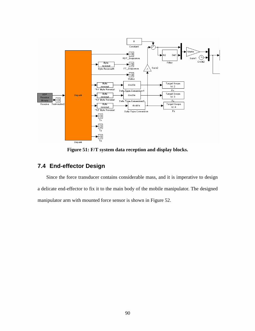
90

Figure 51: F/T system data reception and display blocks.

7.4 End-effector Design

Since the force transducer contains considerable mass, and it is imperative to design

a delicate end-effector to fix it to the main body of the mobile manipulator. The designed

manipulator arm with mounted force sensor is shown in Figure 52.

91

Figure 52: View of manipulator arm with force sensor For a detailed mechanical design, Figure 53 shows an exploded view of the force

sensor system with notations. It is important to ensure sufficient clearances between the

mounted transducer and other fixtures and that total stack height is acceptable. Also make

sure that the user could have access to the mounting screws for attaching the transducer.

The mounting adapter plate is machined for attaching to the robot. All user-supplied

screws must be flush with the inside of the mounting adapter to ensure proper clearance

for the electronics inside the transducer.

92

Transducer

Delrin TipMounting Plate

Bolt

Mounting Adapter

Figure 53: Exploded view of force sensor with notation The other side of the transducer also provides screw slots to mount an end-effector

for manipulation task. In our design, we machined a mounting plate with delrin tip which

would provide compliant contact with the environment to enhance contact stability. The

overall WMM with mounted force sensor is shown in Figure 54

93

Figure 54: WMM with mounted force sensor

7.5 Force Control Simulation

The force control scenario is shown in Figure 56 where a two link manipulator is

regulated to get in contact with a vertical wall. In the simulation test, we would adopt a

hybrid impedance control technique and verify it in the two link manipulator arm. The

task space impedance controller has the following form

= + + + −ɺɺ ɺ ( )d d Ev p fu x k e k e k F F [7.4]

To increase the stability, we add some damping term in the task space and get the

new controller with the form

= + + + − −ɺɺ ɺ ɺ( )d d Ev p f vu x k e k e k F F k x [7.5]

94

0 0.1 0.2 0.3 0.4 0.5 0.6 0.7

0

0.1

0.2

0.3

0.4

0.5

0.6

0.7

Figure 55: Two link manipulator in contact with vertical wall The overall control scheme is implemented in MATLAB SIMULINK using

RealTime xPC TargetTM as shown in Figure 56.

Figure 56: Diagram of xPC Target The simulation result for the contact force profile is shown in Figure 57.

95

0 1 2 3 4 5 6 7 8 9 10-1

0

1

2

3

4

5

6

time(second)

Con

tact

For

ce(N

ewto

n)

desired force

actual force

Figure 57: Force profile under HIC regulation

7.6 Force Sensor and Motor Calibration

0 0.02 0.04 0.06 0.08 0.1 0.12 0.14 0.16 0.18 0.2-2

0

2

4

6

8

10

12

14

16

Data sequence (second)

For

ce (

New

ton)

force with weights

Figure 58: Force reading with 0-5 weights

By varying the number of weights from 0 to 5, we test the static reading of the force

sensor in the –Z direction, as shown in Figure 58. With this static calibration, we can

calibrate the force sensor and find out the software calibration setting.

96

xPC Signal

Motor Controller

Servo Amplifier

Motor

Bit Value Voltage Current Torque

Figure 59: Schematic of motor control implementation With this preparation, we can have a look at the robot hardware implementation.

Since the computed torque would be transformed into bit values which are used are the

direct control signal for the motor controller. It is imperative to find out the mapping from

the computed torque to the real bit-torque value. We consider all the system in the dash

line box as a black box and we can test the output force with different bit value.

(a) (b) Figure 60 : Robot configuration of motor calibration

Our test is performed in the WMM system with the two link part as the test platform.

With the different configuration of the robot arm as shown in Figure 60, we can find out

the bit-torque mapping for motor 1 and motor 2. The calibrated results are illustrated in

Figure 61 (a) and (b).

97

0 50 100 150 200 250 300-4

-3

-2

-1

0

1

2

3

4

bit value

torq

ue (

N.m

)

motor 1 fit line y=-0.0280x+3.4840

0 50 100 150 200 250 300-4

-3

-2

-1

0

1

2

3

4

bit value

torq

ue (

N.m

)

motor 2 fit line y=-0.0271x+3.3803

(a) (b) Figure 61: (a) Calibration of motor 1; (b)Calibration of motor 2

With the calibrated sensor and motor torque, we perform the control routine in the

hardware system and the force control profile is shown in Figure 62. We can see that

there is some force burst in the beginning and there is some noisy signal in the control

process. One important problem is the steady state error.

0 1 2 3 4 5 6 7 8 9 100

0.5

1

1.5

2

2.5

3

3.5

4

4.5

5

Data sequence (second)

For

ce (

New

ton)

force with weights

Figure 62: Experiment force data

98

8 Conclusion and Future Work

8.1 Summary

In Chapter 1, we reviewed some related works on mobile manipulator collectives,

from the multiple agent robots, multiple finger hand and multiple legged robots. We

analyzed the related issues in the cooperative control systems.

Chapter 2 discussed a variety of preliminary knowledge on modeling and control of

constrained mechanical systems. Some detailed background theory includes operational

space dynamics and control, constrained Lagrange dynamics.

Chapter 3 is about the force control review, and because the focus of this thesis is on

force control of manipulators, we will introduce and categorize some popular force

control schemes developed since three decades ago in. We will also highlight the benefits

and limitations of some approaches and show some empirical and visionary perspective

basing on the existing experiment results and some related literature.

Chapter 4 focuses on the modeling and control of WMMs. We begin by investigating

the kinematic and dynamic model of WMR, and then the similar analysis would be

performed in the WMM system with a focus on task space consistent dynamic control

method. As a main body of this thesis, the multiple grasp modeling would be investigated

therein and the decentralized control of WMM collectives would be presented in this

chapter.

Chapter 5 investigates the formation control of a group of WMMs. The mobile robot

formation problem is investigated first for a basic study, and this problem is split into

trajectory tracking and static obstacle avoidance, formation control and cooperative

99

obstacle avoidance. All of these results are generalized to mobile manipulator cases.

Chapter 6 presents simulation results for various interesting cases studies using the

dynamic equation formulated in Chapter 3. In particular, the first two case studies were

performed for the dynamic payload transport scenario. The subsequent two cases were

targeted at mobile manipulator collective formation control.

Chapter 7 introduces the experimental setup and verification procedure. A force

sensor calibration and manipulator torque calibration method is proposed therein.

8.2 Future Work

Force Control Algorithm One of the difficult issues met in the experiment is that the system is quite sensitive

to control parameters. One remedy is to perform delicate system identification, but it is

necessary to note that some dynamic effects like the Coulomb friction is difficult or

impossible to be identified, and even these models are perfected obtained, a stable

controller is still an important problem to be solved.

Force Signal Processing In our implementation, the sensed signal is filtered through a first order low pass

filter, but in fact, the sensed data also contains the sensors acceleration, environment

disturbance and some noise. Some researchers have begun to study these problems and

have proposed some algorithms. The application of these algorithms into WMM is still

rare.

Force Control Implementation on WMM Since the system modeling problem, our system is still too sensitive to control

parameter, so the force control implementation on WMM still needs further investigation.

100

Reference

[1] Y. U. Cao, A. S. Fukunaga, A. B. Kahng, and F. Meng, "Cooperative mobile robotics: Antecedents and directions," Pittsburgh, PA, USA, 1995, pp. 226-234.

[2] T. Arai, E. Pagello, and L. E. Parker, "Editorial: Advances in Multi-Robot Systems," IEEE Transactions on Robotics and Automation, vol. 18, pp. 655-661, 2002.

[3] C. Reynolds, "Flocks, Herds, and Schools: A Distributed Behavioral Model " in ACM SIGGRAPH '87 Conference Proceedings, Anaheim, California, 1987.

[4] T. L. Huntsberger, A. Trebi-Ollennu, H. Aghazarian, P. S. Schenker, P. Pirjanian, and H. D. Nayar, "Distributed control of multi-robot systems engaged in tightly coupled tasks," Autonomous Robots, vol. 17, pp. 79-92, 2004.

[5] A. Nakamura, J. Ota, and T. Arai, "Human-supervised multiple mobile robot system," IEEE Transactions on Robotics and Automation, vol. 18, pp. 728-43, 2002.

[6] J. K. Salisbury and J. J. Craig, "Articulated hands: force control and kinematic issues," Charlottesville, VA, USA, 1981, pp. 2-1.

[7] V. Kumar and K. J. Waldron, "Force distribution in closed kinematic chains," Philadelphia, PA, USA, 1988, pp. 114-19.

[8] S. Arimoto, F. Miyazaki, and S. Kawamura, "Cooperative motion control of multiple robot arms or fingers " in IEEE International Conference on Robotics and Automation., 1987.

[9] O. Khatib, "Inertial properties in robotic manipulation. An object-level framework," International Journal of Robotics Research, vol. 14, pp. 19-36, 1995.

[10] M. Zribi and S. Ahmad, "Predictive adaptive control of multiple robots in cooperative motion," in Proceedings of the 30th IEEE Conference on Decision and Control, 1990.

[11] K. T. Kosuge, D.; Fukuda, T.; Sakai, M.; Kanitani, K., "Decentralized coordinated motion control of manipulators with vision and force sensors

" in Proceedings of IEEE International Conference on Robotics and Automation, 1995. [12] K. O. Kosuge, T.; Seki, H., "Decentralized control of multiple manipulators handling an objectin

coordination based on impedance control of each arm," in Proceedings of IEEE/RSJ International Conference on Intelligent Robots and Systems, 1997.

[13] Y.-H. Liu and S. Arimoto, "Decentralized adaptive and nonadaptive position/force controllers for redundant manipulators in cooperations," International Journal of Robotics Research, vol. 17, pp. 232-47, 1998.

[14] J. Szewczyk, F. Plumet, and P. Bidaud, "Planning and controlling cooperating robots through distributed impedance," Journal of Robotic Systems, vol. 19, pp. 283-97, 2002.

[15] G. Montemayor and J. T. Wen, "Decentralized collaborative load transport by multiple robots," Barcelona, Spain, 2005, pp. 372-377.

[16] J. P. Desai and V. Kumar, "Motion planning for cooperating mobile manipulators," Journal of Robotic Systems, vol. 16, pp. 557-79, 1999.

[17] H. G. Tanner, S. G. Loizou, and K. J. Kyriakopoulos, "Nonholonomic navigation and control of cooperating mobile manipulators," IEEE Transactions on Robotics and Automation, vol. 19, pp. 53-64, 2003.

[18] Y. Kume, Y. Hirata, Z.-D. Wang, and K. Kosuge, "Decentralized control of multiple mobile manipulators handling a single object in coordination

" in IEEE/RSJ International Conference on Intelligent Robots and System, 2002. [19] Y. K. Hirata, Y.; Sawada, T.; Zhi-Dong Wang; Kosuge, K., "Handling of an object by multiple

mobile manipulators in coordination based on caster-like dynamics " in IEEE International Conference on Robotics and Automation 2004. [20] Y. K. Hirata, K., "Coordinated motion control of multiple robots without positioninformation of

each robot " in Proceedings of the 39th IEEE Conference on Decision and Control 2000. [21] O. Khatib, K. Yokoi, K. Chang, D. Ruspini, R. Holmberg, and A. Casal, "Coordination and

decentralized cooperation of multiple mobile manipulators," Journal of Robotic Systems, vol. 13,

101

pp. 755-64, 1996. [22] J. Tan and N. Xi, "Integrated Task Planning and Control for Mobile Manipulators," International

Journal of Robotics Research, vol. 22, pp. 337-354 2003. [23] R. Bhatt, C. P. Tang, M. Abou-Samah, and V. Krovi, "A screw-theoretic analysis framework for

payload manipulation by mobile manipulator collectives," Orlando, FL, United States, 2005, pp. 1597-1606.

[24] M. Abou-Samah, C. P. Tang, and R. M. B. V. Krovi, "A kinematically compatible framework for cooperative payload transport by nonholonomic mobile manipulators," Autonomous Robots, vol. 21, pp. 227-242, 2006.

[25] R. W. Brockett, "Asymptotic Stability and Feedback Stabilization," in Differential Geometric Control Theory, R. S. M. R. W. Brockett and a. H. J. Sussmann, Eds.: Boston, MA: Birkhauser, 1983, pp. 181-191.

[26] O. Khatib, "A unified approach for motion and force control of robot manipulators: the operational space formulation," IEEE Journal of Robotics and Automation, vol. RA-3, pp. 43-53, 1987.

[27] J. Park and O. Khatib, "A haptic teleoperation approach based on contact force control," International Journal of Robotics Research, vol. 25, pp. 575-91, 2006.

[28] V. De Sapio, O. Khatib, and S. S. Delp, "Task-level approaches for the control of constrained multibody systems

" Multibody System Dynamics, vol. 16, pp. 73-102, 2006. [29] E. L. Faulring, K. M. Lynch, J. E. Colgate, and M. A. Peshkin, "Haptic display of constrained

dynamic systems via admittance displays," IEEE Transactions on Robotics, vol. 23, pp. 101-11, 2007.

[30] N. Hogan, "IMPEDANCE CONTROL: AN APPROACH TO MANIPULATION: PART III - APPLICATIONS," Journal of Dynamic Systems, Measurement and Control, Transactions ASME, vol. 107, pp. 17-24, 1985.

[31] Y. Shen and K. Huper, "A joint space formulation for compliant motion control of robot manipulators," Niagara Falls, Ont., Canada, 2005, pp. 362-9.

[32] M. H. Raibert and J. J. Craig, "Hybrid position/force control of manipulators," Transactions of the ASME. Journal of Dynamic Systems, Measurement and Control, vol. 103, pp. 126-33, 1981.

[33] C. H. An and J. M. Hollerbach, "Kinematic stability issues in force control of manipulators," Raleigh, NC, USA, 1987, pp. 897-903.

[34] R. Holmberg and O. Khatib, "Development and control of a holonomic mobile robot for mobile manipulation tasks," International Journal of Robotics Research, vol. 19, pp. 1066-74, 2000.

[35] G. Campion, G. Bastin, and B. D'Andrea-Novel, "Structural Properties and Classification of Kinematic and Dynamic Models of Wheeled Mobile Robots," IEEE Transactions on Robotics and Automation, vol. 12, pp. 47-62, February 1996.

[36] J. Borenstein, B. Everett, and L. Feng, Navigating Mobile Robots: Systems and Techniques. Wellesley, MA: A. K. Peters, Ltd., 1996.

[37] J. Angeles, Fundamentals of Robotic Mechanical Systems: Theory, Methods, and Algorithms Springer, 2003.

[38] V. Kumar, X. Yun, E. Paljug, and N. Sarkar, "Control of contact conditions for manipulation with multiple robotic systems," Sacramento, CA, USA, 1991, pp. 170-5.

[39] R. Murray, Z. Li, and S. Sastry, A Mathematical Introduction to Robotic Manipulation: CRC Press, 1994

[40] D. Williams and O. Khatib, "The virtual linkage: a model for internal forces in multi-grasp manipulation," Atlanta, GA, USA, 1993, pp. 1025-30.

[41] K. Kosuge and Y. Hirata, "Coordinated Motion Control of Multiple Manipulators," in Robotics and Automation Handbook, T. Kurfess, Ed.: CRC Press, 2005.

[42] T. Balch and R. C. Arkin, "Behavior-based formation control for multirobot teams," IEEE Transactions on Robotics and Automation, vol. 14, pp. 926-39, 1998.

[43] H. G. Tanner, "ISS properties of nonholonomic vehicles," Systems &amp; Control Letters, vol. 53, pp. 229-35, 2004.

[44] S. Mastellone, D. M. Stipanovic, and M. W. Spong, "Remote formation control and collision avoidance for multi-agent nonholonomic systems," Roma, Italy, 2007, p. 6 pp.

[45] S. Mastellone, D. M. Stipanovic, C. R. Graunke, K. A. Intlekofer, and M. W. Spong, "Formation control and collision avoidance for multi-agent non-holonomic systems: Theory and experiments,"

102

International Journal of Robotics Research, vol. 27, pp. 107-126, 2008. [46] G. Leitmann and J. Skowronski, "Avoidance control," Journal of Optimization Theory and

Applications, 1977. [47] I. ATI Industrial Automation, "ATI Net F/T Manual," Apex, NC, 2007.

103

Appendix

Mechanical Design

This section includes the mechanical drawings for all the parts needed to construct

the physical prototype. The solid models and drawings were created using Solid Works

Educational Edition 2006.

104

105

106

107

108

109