Hard x-ray observations of the extragalactic sky: the High

Energy Focusing Telescope and the Serendipitous

Extragalactic X-ray Source Identification survey

Thesis by

Peter Hsih-Jen Mao

In Partial Fulfillment of the Requirements

for the Degree of

Doctor of Philosophy

California Institute of Technology

Pasadena, California

2002

(Submitted May 24, 2002)

ii

c© 2002

Peter Hsih-Jen Mao

All Rights Reserved

iii

Acknowledgments

You learn what you don’t know you are learning.

—Gian-Carlo Rota

Luck comes to the well prepared.

—Steven Frautschi

As an undergraduate, I was told that one’s graduate school experience is far more

dependent on the advisor than the school itself. Indeed, I have had a wonderful time here,

and I attribute much of it to my advisor, Fiona Harrison. In my first few weeks at Caltech,

I took David Hogg’s advice to talk to many different professors before picking a research

group. Tom Prince told me about a project to design high energy x-ray mirrors that Fiona,

who was in Australia flying a balloon, would be taking the lead on. The project sounded

interesting to me, but, having never met her, I had no idea how Fiona would be as an

advisor and she had no idea how I would be as a student. Tom relayed my interest in the

project to her, she agreed to take me as a student, and things have worked out pretty well.

Fiona has given me opportunities to meet and work with many talented, interesting and

fun scientists all over the world. She has given me the leeway to develop my own style of

doing science, while at the same time making sure that my graduate education has been

well rounded. I have copious tales of her generosity, but they would only serve to embarrass

her.

My first trip with Fiona was to the Motor City, to begin multilayer fabrication tests

with Osmic, Inc. There, I worked with Yuriy Platonov, Luis Gomez, David Broadway, and

Brian DeGroot (who left Osmic to take over his family’s pig farm in Canada). All of the

mirror fabrication that I directly had a hand in happened at Osmic with Yuriy, Luis, David,

and Brian, and I thank them for their patience, hospitality, and generosity in sharing their

knowledge and experience. I remember remarking to Fiona on that first trip that I thought

Detroit would be an interesting place to live. She didn’t agree.

During my second trip to Osmic, I took some time to visit the Henry Ford Museum in

Dearborn, where I saw the Aston Martin DB5 from the James Bond movies. The DB5 was

iv

stolen from a Boca Raton airport later that year.

The Danish Space Research Institute is part of the HEFT collaboration, responsible

for the coating of the flight optics. Our cohorts in Denmark include Finn Christensen, the

Danish cowboy, Ahsen Hussain, his incorruptible graduate student, and Carsten Jensen, his

very corruptible post-doc. A few weeks after Deirdre and I got married, Fiona sent me off

to Denmark to characterize some mirrors that we had coated at Osmic. Finn thought this

was a bad idea, since the last time a collaborator had come to Copenhagen, the collaborator

broke off his engagement. Deirdre and I are still married. On that trip, I worked with Ahsen,

Karsten Joensen, Finn’s former student on whose work mine builds, and the Italians Carlo

Pelliciari and Giovanni Pareschi. Giovanni has a great story about an encounter he had

with a stranger in Lyon, France.

Copenhagen is the home of Hans Christian Andersen and one of its landmarks is the

statue of the Little Mermaid. I visited the site of the statue on Thanksgiving. After I

returned to the States, I heard that some vandals had cut her head off.

At the 1998 Physics of X-ray Multilayer Structures conference in Breckenridge, CO, I

first met David Windt, at the time a researcher at Bell Laboratories. David invited me to

work with him for a few weeks at Bell Labs. This was a key event in my graduate career.

Following discussions with David, I reorganized my approach to multilayer design and this

eventually led to the figure of merit and optimization methods described in this thesis.

David has since left Bell Labs to join the HEFT collaboration at Columbia University.

The multilayer optimization software also owes its existence to Tom Prince, Stuart

Andersen, and Leon Bellan. Tom helped me get access to the Caltech Advanced Computing

Resource’s massively parallel supercomputers and Stuart showed me the ins and outs of

parallel computing. In the summer of 1999, I was lucky to procure the services of a pre-

frosh Summer Undergraduate Research Fellowship (SURF) student, Leon Bellan. Leon

implemented the iterative search routine into the multilayer optimization program, allowing

it to make full and efficient use of the parallel computers. The great thing about Leon is

that, besides being fun to hang around with, he finished the project way ahead of time, so

I had to give him other things to do.

As an undergraduate at MIT, I took a class on Phenomenology, a branch of philosophy

developed by the likes of Husserl, Heidegger, and Wittgenstein. Gian-Carlo Rota taught the

class, and one of the phenomena that he described was called “falling.” Basically, it is the

v

angst that one feels upon completing some project or upon reaching some goal. Anyways,

I experienced “falling” after figuring out how to optimize telescope mirror designs and told

Fiona that I wanted to work on something different. Much to my delight, Hubert Chen has

taken over the multilayer optimization work. Hubert has thoroughly learned all the nuances

of multilayer design and is well poised to further develop the code.

“Something different” turned out to be the SEXSI survey. Fiona and David Helfand

at Columbia University had been talking about using Caltech and Columbia’s vast optical

observing resources to conduct a wide-area optical follow-up survey of x-ray sources de-

tected by the soon-to-be-launched Chandra X-ray Observatory. Fiona and David coined

the acronym “SEXSI” during the Y2K observing run at Palomar. Apparently, the name

stuck because David’s wife, Jada Rowland, expressed her doubts that they would use such

a provocative name for the project.

The SEXSI survey put me in contact with another set of great people: Alan Diercks,

David Kaplan, Elise Laird, Jeff Blackburne, Dan Stern, and Megan Eckart. I inherited

a lot of the optical reduction software for SEXSI from Alan with considerable help from

David Kaplan. Alan taught me the crucial practice electronically logging all of my data

reduction commands and I greatly appreciate our long, in-depth discussions about the role

of astronomy and astrophysics in society. Alan is now at the Institute for Systems Biology

in Washington and his work is closer to Deirdre’s than it is to mine. Elise took over most of

the optical imaging data reduction from me last year when the spectroscopic data became

overwhelming. Elise is the most meticulous scientist that I have worked with and I wish

her the best in her impending graduate education at Imperial College London. Jeff spent

last summer as a SURF student working out the many bugs in LFC data reduction. Jeff

produced a working data reduction pipeline with virtually no supervision from me. Like

Leon, he is an example of Caltech’s ability to attract hyper-talented undergrads. Dan

brought to SEXSI much-needed expertise in multislit spectroscopic data reduction. I would

probably still be struggling with SEXSI’s mountains of spectroscopic data had Dan not taken

an interest in this project. Over the past year, as I went into thesis-writing hibernation,

Megan took over my role in the SEXSI survey. Megan’s dedication to the project cannot

be questioned – unlike most of us, she has bled for Science, risking life and limb to make

sure data tapes from observing runs come back to Caltech safely.

vi

Oh, come on, it’s a big American car with a V8!

—Deirdre Scripture-Adams (1996)

Coming to Los Angeles at the ripe age of 23, I suffered considerable culture shock: the

cars, the highways, the smog . . . the cars. I got hooked pretty early. Stephane Corbel, a

visiting French student, was returning home and had a car to sell – 1978 Dodge Aspen, 318

CID, 4 barrel carb, $800. I didn’t want it. Deirdre insisted. She won, and I fell in love with

the internal combustion engine. I was in denial for the longest time, but my officemates,

Brian Matthews, Derrick Key and Alan Labrador, saw it from a mile away. About a year

after we bought the Aspen, I pulled the heads because the distributor cap needed to be

replaced. Now, anyone who knows cars, knows that you don’t need to pull the heads to

replace a distributor cap. Regardless, the whole point of this is that while ripping that 318

apart, I got to know two really cool car-guys: Lou Madsen and John Yamasaki. Lou and I

have spent countless hours doing “car-appreciation.” Lou’s powers of automotive diagnosis

are legendary, as are his driving skills.

Six months after acquiring the Aspen, I went looking for a 1966 Mustang. Derrick Key,

who has a ’66 convertible Mustang, went looking with me and we found a mostly-straight

’66 coupe from a biker in the Valley. The woman who picked up the phone when I called

said something like, “Oh he’s real nice – doesn’t even get into fights that much!” The night

we went to pick up the car was rather bizarre. I will not recount the story here. After

I passed my candidacy exam in 1998, I celebrated by pulling the Mustang’s engine and

having a new, punched-out 302 built by Steve Fekete (Hollywood Machine Shop, Pasadena,

CA). Steve is a Bowtie-guy, but he did wonders with that Blue-oval mill. John Yamasaki

was instrumental in both the extraction of the old engine and the installation of the new

one, providing lifts, stands, a truck, and his lower back to complete the job. Many thanks

to Fiona for putting up with me assembling the new engine in my office.

Which brings me to the third car. Here, I am tempted to gush because the car means a

lot to me, but, in deference to Fiona’s matter-of-fact style, I will just state the facts. Fiona

owned a 1972 BMW 2002 from her days as a grad student at Berkeley. She no longer drove

nor worked on the car anymore and wanted the car to go to someone who would appreciate

it. I love cars. Voila. Thanks, Fiona!

Before I get off the subject of cars, I must apologize to John Cortese, my officemate and

vii

fellow Bostonian, for opening that can of carb cleaner in the office. John demonstrated to

me, by example, that the ultimate goal in life is not to acquire riches or fame, but to collect

a wide variety of stories. Knee slappers, jaw droppers, tales of woe and anguish, John has

them all and I’m sure that the ones I’ve heard only scratch the surface.

For all but my first year in grad school, I lived 23 miles from campus, in West L.A. I

most certainly would have gone completely insane, had it not been for my fellow carpoolers:

Georgia de Nolfo, Deborah Goodman, Cara-Lou Stemen, Mike Zittle, Lou Madsen, and

Mark Bartelt. Far, far too many stories to tell here.

Luck, indeed, does come to the well prepared, and I am grateful those who prepared me

for Caltech. Mom and Dad came to the U.S. as graduate students and raised me, Mike and

Julie in the suburbs outside of Boston. I am who they made me, and I am always thankful

of that. My interest in x-rays is due to Lee Grodzins and Chuck Parsons. I had Lee for

“Junior Lab” and when I finished MIT, he hired me to work at his company, Niton. Lee’s

outlook on Science and his enthusiasm for the work have had a deep influence on me. Chuck

was my boss at Niton. He had great confidence in my abilities, and I had great appreciation

for his knowledge and wisdom. Rest in peace, Chuck.

I end this long, rambling acknowledgement with one for Deirdre Scripture-Adams, the

girl I met during our first week at MIT. Like Lee has said of his wife, Lulu, I only wish that

I had met her sooner.

viii

Abstract

Extending the energy range of high sensitivity astronomical x-ray observations to the hard

x-ray band (10–100 keV) is important for the study of nonthermal emission mechanisms

and heavily obscured sources. This thesis, in two parts, describes the development of the

High Energy Focusing Telescope (HEFT), a focusing telescope for the hard x-ray band, and

the Serendipitous Extragalactic X-ray Source Identification (SEXSI) survey, a degree-scale

x-ray/optical survey of sources detected in the Chandra hard band (2–7 keV).

HEFT is a balloon-borne x-ray telescope that is expected to have its first flight in the

fall of 2003. The telescope will be among the first to focus x-rays at energies greater than 20

keV. HEFT’s mirrors use graded multilayers – thin film coatings (∼ 1µm) that enhance high

energy reflectance via constructive interference. In the first half of the thesis, I describe the

optimization algorithm that I developed for x-ray optics and how I applied this algorithm

to the design of the HEFT optics. In addition, I present x-ray measurements that verify

the HEFT multilayer coating designs at energies where the telescope will operate.

The SEXSI survey complements Chandra deep-field surveys by covering a much larger

area of the sky, but to a shallower x-ray flux limit. For the SEXSI survey, we use public

data from the Chandra archive to compile a catalog of extragalactic sources detected in

the 2–7 keV band. We identify the optical counterparts to the x-ray sources and obtain

their optical spectra (400–1000 nm). Presently SEXSI includes 30 Chandra fields, covering

roughly 2 square degrees and yielding over 1200 x-ray sources to a flux limit of 10−15–10−13

erg cm−2 s−1. In the second part of the thesis, I present results from 10 fields for which we

have substantial spectroscopic coverage.

ix

Contents

Acknowledgments iii

Abstract viii

1 Introduction 1

2 Overview of the High Energy Focusing Telescope 7

2.1 Payload overview . . . . . . . . . . . . . . . . . . . . . . . . . . . . . . . . . 8

2.1.1 Detectors . . . . . . . . . . . . . . . . . . . . . . . . . . . . . . . . . 9

2.1.2 Optics . . . . . . . . . . . . . . . . . . . . . . . . . . . . . . . . . . . 10

3 Principles of x-ray multilayers 14

3.1 X-ray reflection from standard materials . . . . . . . . . . . . . . . . . . . . 14

3.2 X-ray reflectivity from multilayers . . . . . . . . . . . . . . . . . . . . . . . 16

3.3 General design considerations . . . . . . . . . . . . . . . . . . . . . . . . . . 18

3.3.1 Bilayer thickness range . . . . . . . . . . . . . . . . . . . . . . . . . . 18

3.3.2 Bilayer thickness distribution . . . . . . . . . . . . . . . . . . . . . . 19

3.4 Multilayer materials . . . . . . . . . . . . . . . . . . . . . . . . . . . . . . . 21

4 Optimization of multilayer designs 24

4.1 Geometry of the optics . . . . . . . . . . . . . . . . . . . . . . . . . . . . . . 24

4.2 Effective areas . . . . . . . . . . . . . . . . . . . . . . . . . . . . . . . . . . 26

4.2.1 Geometry-dependent area . . . . . . . . . . . . . . . . . . . . . . . . 27

4.2.2 Transmission components of the effective area . . . . . . . . . . . . . 29

4.3 Figure of merit function . . . . . . . . . . . . . . . . . . . . . . . . . . . . . 30

4.4 Design optimization . . . . . . . . . . . . . . . . . . . . . . . . . . . . . . . 31

4.4.1 Parameterization of the bilayer distribution . . . . . . . . . . . . . . 31

4.4.2 Bilayer thickness range . . . . . . . . . . . . . . . . . . . . . . . . . . 32

4.4.3 Optimization algorithm, characteristics of the FOM surface . . . . . 34

4.5 The HEFT optimization . . . . . . . . . . . . . . . . . . . . . . . . . . . . . 36

x

4.5.1 Results of the optimization for HEFT . . . . . . . . . . . . . . . . . 38

4.6 Further developments in optimization . . . . . . . . . . . . . . . . . . . . . 41

5 Multilayer fabrication 44

5.1 Deposition systems . . . . . . . . . . . . . . . . . . . . . . . . . . . . . . . . 45

5.2 High-energy measurements of graded multilayer designs . . . . . . . . . . . 46

6 The Serendipitous Extragalactic X-ray Source Identification survey 52

7 Data reduction 55

7.1 X-ray reduction . . . . . . . . . . . . . . . . . . . . . . . . . . . . . . . . . . 55

7.2 Optical reduction . . . . . . . . . . . . . . . . . . . . . . . . . . . . . . . . . 59

7.2.1 Imaging . . . . . . . . . . . . . . . . . . . . . . . . . . . . . . . . . . 61

7.2.2 Spectroscopy . . . . . . . . . . . . . . . . . . . . . . . . . . . . . . . 62

8 Results from the SEXSI survey 64

8.1 Spectroscopic classification . . . . . . . . . . . . . . . . . . . . . . . . . . . 64

8.2 Preliminary results from SEXSI . . . . . . . . . . . . . . . . . . . . . . . . . 67

8.2.1 Comparisons with deep-field surveys . . . . . . . . . . . . . . . . . . 68

8.2.2 Emission line galaxies . . . . . . . . . . . . . . . . . . . . . . . . . . 74

8.3 The future of SEXSI . . . . . . . . . . . . . . . . . . . . . . . . . . . . . . . 75

9 Conclusion 77

Bibliography 79

A HEFT optimization results 86

xi

List of Figures

2.1 The sensitivity of HEFT for observations from a balloon platform (left) com-

pared to the large-area coded aperture instruments GRIP and GRATIS, and

from a satellite platform (right) shown relative to current and future x-ray

and gamma-ray instruments. The energy bandwidth is ∆E/E = 50%, and

the balloon observations assume an atmospheric column depth of 3.5 g cm−2. 8

2.2 Schematic diagram of the HEFT payload. . . . . . . . . . . . . . . . . . . . 9

2.3 Top: The HEFT optic mounting and alignment procedure. Bottom: HEFT

uncoated prototype optic on the mounting assembly fixture. . . . . . . . . . 13

3.1 Schematic diagram of a multilayer coating with notation corresponding to

that used in the text. Layers and interfaces are labeled by j, n is the complex

index of refraction, t is the layer thickness, and σ is the interface width.

Adapted from Joensen, 1995. . . . . . . . . . . . . . . . . . . . . . . . . . . 17

3.2 Calculated reflectivity vs. photon energy at 1.75 mrad of a graded W/Si

multilayer and a Cu/Si multilayer with the exact same specifications (bilayer

thickness distribution and interface width). The Cu/Si reflectivity demon-

strates that the range in bilayer thicknesses for this mirror would allow re-

flectivity at 1.75 milliradian from 20 to 100 keV, but the jump in absorption

at the W K-edge (69.5 keV) drastically reduces reflectivity of the W/Si mul-

tilayer above the absorption edge. . . . . . . . . . . . . . . . . . . . . . . . . 22

4.1 Geometry of conical-approximation Wolter I optics with primary and sec-

ondary reflection angles for on- and off-axis rays. . . . . . . . . . . . . . . . 26

4.2 Angularly averaged collecting area vs. radial gap between mirror shells. Vari-

able gap results (+) are plotted against the bottom scale and constant gap

results (×) are plotted against the top scale. Each area is determined by ray

tracing 108 events uniformly distributed in off-axis angles between 0 and 3

mrad, and uniformly distributed spatially over the 12 cm radius aperture.

The standard deviation in the estimate of the area is 0.025 cm2. . . . . . . 27

xii

4.3 Upper left: The two-dimensional reflection angle distribution, Winc(α =

5 mrad, ψ1, ψ2). Because the distribution is nonzero only near the line ψ1 =

−ψ2, it is mapped as ψ1 + ψ2 vs. ψ1. Each contour line demarcates a factor

of ten in the magnitude of the weighting function. Upper right: Projection

of the distribution onto the ψ1 + ψ2 axis. One half of the distribution lies

within 0.625 µrad of ψ1 + ψ2 = 0 and 90% of the distribution lies with 7.5

µrad. Lower left: Projection of the distribution onto the ψ1 axis, Winc(α =

5 mrad, ψ1). . . . . . . . . . . . . . . . . . . . . . . . . . . . . . . . . . . . . 29

4.4 Figure of merit contour maps of a Joensen parameterized graded multilayer.

The dotted lines represent an N = 200 surface and the solid lines represent

an N = 250 surface. The calculations were performed for HEFT’s innermost

set of mirror shells. . . . . . . . . . . . . . . . . . . . . . . . . . . . . . . . . 35

4.5 Figure of merit vs. coating thickness for HEFT’s α = 2.32–2.59 mrad mirrors.

The dashed lines indicate levels of 98% and 95% of the optimum figure of

merit. σ is the RMS interface width. . . . . . . . . . . . . . . . . . . . . . . 39

4.6 Angularly averaged effective area and energy weighted, angularly averaged

effective area (in bold). WE ∝ E[keV + 70]. The solid line, N = 233, corre-

sponds to the HEFT design with a figure of merit that is 98% of optimum.

The dashed line, N = 363, is our best estimate of optimum design. The fig-

ure of merit is the average value of the energy weighted, angularly averaged

effective area. . . . . . . . . . . . . . . . . . . . . . . . . . . . . . . . . . . . 40

4.7 Mirror group 4 effective areas at 0.0, 0.5, 1.0, and 1.5 mrad off axis. The

98% optimum design (N = 233) is shown with heavy lines and the optimum

design (N = 363) is shown with light lines. . . . . . . . . . . . . . . . . . . 41

4.8 Effective area of the full 14-module HEFT design for on-axis sources and

off-axis point sources at 0.5, 1.0, and 1.5 mrad off-axis. . . . . . . . . . . . . 42

5.1 Recent results of thickness uniformity measurements from the DSRI pro-

duction coating facility. In the original baseline tests performed at Osmic,

the coating thickness fit a cosine function in the azimuthal direction (dotted

lines). The latest results from DSRI demonstrate considerable improvement

in the uniformity of the coatings. . . . . . . . . . . . . . . . . . . . . . . . . 47

xiii

5.2 Data and model as described in the text for all mirror segments at 34 keV

and φ = +5. The full line is the model calculation. . . . . . . . . . . . . . 49

5.3 Data and model as described in the text for all mirror segments at 65 keV

and φ = −8. The full line is the model calculation. . . . . . . . . . . . . . 50

5.4 Data and model as described in the text for mirror segment D3 at 170 keV and

D4 at 158 keV. In both cases, the azimuthal position is φ = −8. The solid

lines show the calculated reflectivity vs. incidence angle assuming σ = 4.5A.

The dotted lines are calculated reflectivities for σ = 4.2A (D4, 158 keV) and

σ = 4.8A (D3, 170 keV). . . . . . . . . . . . . . . . . . . . . . . . . . . . . . 51

6.1 Exposure time distribution of the SEXSI survey. The heavy line shows the

exposure times of the 10 fields for which we have optical spectroscopic data. 53

7.1 ACIS flight focal plane layout. Courtesy of Chandra Science Center [1]. . . 56

7.2 Chandra effective area for front- and back-side chips. Courtesy of Chandra

Science Center [1]. . . . . . . . . . . . . . . . . . . . . . . . . . . . . . . . . 57

7.3 A pathological case demonstrating problems with wavdetect’s determination

of source positions. Left: NGC 1569, chip 2, hard-band CXO image. Data

courtesy of Crystal Martin. Right: P60, CCD-13 R band image of the same

field. The green circles mark the wavdetect positions. The blue markers

indicate centroid positions that do not meet the criteria to supersede the

wavdetect positions and red markers indicate positions where the centroid

position supersedes the wavdetect position. The radii of the markers corre-

spond to the PSF of the mirror array at that location. The north arm of the

compass rose is 60′′ and the east arm is 30′′. . . . . . . . . . . . . . . . . . . 58

xiv

7.4 More typical source position results from wavdetect. Here, source c6007 has

the largest ∆r2/PSF offset, at 0.21, followed by c6005 with a 0.20 offset.

Both are well below our criteria for using centroid-derived positions. Left:

HCG 62, chip 6, hard-band CXO image. Data courtesy of Jan Vrtilek. Right:

MDM 2.4 m, Eschelle camera R band image of the same field. The green

circles mark the wavdetect positions. The blue markers indicate centroid

positions. The radii of the markers correspond to the PSF of the mirror

array at that location. The north arm of the compass rose is 60′′ and the

east arm is 30′′. . . . . . . . . . . . . . . . . . . . . . . . . . . . . . . . . . . 59

7.5 ∆r2/PSF vs. wavdetect derived SNR for hard-band detections from NGC

1569, chip 2 and HCG 62, chip 6. The dotted line indicates the cut, above

which we adopt the centroid derived position . . . . . . . . . . . . . . . . . 60

8.1 Example of a low redshift broad line AGN with broad Hα and Hβ lines. The

source is a7007 from the 3C 295 field. The permitted Mg and H lines exceed

3800 km/s FWHM. The redshift of the source is 0.4719 ± 0.0009. Here and

in the following spectra, the ⊕ symbol indicates telluric night-sky lines. . . 65

8.2 Example of a broad line AGN from the GRB 010222 field, source b6007. The

redshift of the source is 1.609 ± 0.003. . . . . . . . . . . . . . . . . . . . . . 65

8.3 Example of a narrow line AGN from the HCG 62 field, source c7022. The

widths of the permitted emission lines are at resolution limit of the spectro-

graph. The redshift of the source is 1.154 ± 0.002. . . . . . . . . . . . . . . 66

8.4 Example of an emission line galaxy from the GRB 000926 field, source b3004.

The red-side flux has been multiplied by 1.4 to compensate for a discepancy

in the flux calibration between the red and blue cameras. The redshift of the

source is 0.2587 ± 0.0006. . . . . . . . . . . . . . . . . . . . . . . . . . . . . 66

8.5 Example of an absorption line galaxy from the NGC 1569 field, source d3008.

The redshift of the source is 0.753 ± 0.001. . . . . . . . . . . . . . . . . . . . 67

xv

8.6 Hardness ratio, (H–S)/(H+S), vs. soft (0.5 – 2.1 keV, left panel) and hard

(2.1 – 10.0 keV, right panel) band fluxes. The sources are taken from the ten

fields for which we have optical spectroscopic data. The vertical scales for

both plots are the same; the equivalent photon index scale is shown on the

right hand side of the hard-band plot. . . . . . . . . . . . . . . . . . . . . . 68

8.7 Top panel: hardness ratio, (H+S)/(H-S), vs. redshift. The right-hand scale

shows the equivalent photon index. The dotted lines trace the hardness ratio

vs. redshift of a source with a Γ = 1.7 spectrum, intrinsically obscured by

NH column densities of 1020, 1021, 1022, and 1023 cm−1. The solid dots

indicate sources with low ratios of soft-band x-ray flux to optical R band

flux. Bottom panel: redshift distributions of broad and narrow line AGN,

emission line galaxies, and normal galaxies found in the SEXSI survey. . . . 70

8.8 Hardness ratio distributions of broad and narrow line AGN, emission line

galaxies, normal galaxies and optically faint, uncategorized objects. The

plots have been slightly shifted to avoid overlapping. On average, emission

line galaxies have the hardest x-ray spectra and broad line AGN have the

softest spectra. Narrow line AGN and normal galaxies appear to be evenly

distributed over the observed -0.6 to 1.0 hardness ratio range. Based on these

distributions, the optically faint sources do not appear to be dominated by

either broad line AGN or emission line galaxies. . . . . . . . . . . . . . . . . 71

8.9 Hardness ratio vs. soft-band (left) and hard-band (right) luminosities. Con-

trary to the results of the CDF-S, we find considerable overlap among the

different categories of sources. As in the case of HR vs. flux, we find that

hardness increases with decreasing soft-band luminosity, but that the corre-

lation with hard-band luminosity is much weaker. . . . . . . . . . . . . . . . 72

xvi

8.10 (a) Soft-band (0.5 – 2.1 keV) and (b) Hard-band (2.1 – 10.0 keV) x-ray to

optical (R band) flux ratios vs. the respective x-ray band flux. The dashed

lines indicate lines of constant optical flux, at mR = 24 and mR = 25. In

general, we do not spectroscopically pursue sources with mR > 24. Sources

with low soft x-ray to optical flux ratios (< −1.5) are marked with a solid

dot. The Ms surveys only observe these sources at soft fluxes below 10−15 erg

s−1 cm−2. SEXSI, and EMSS before, demonstrate that the optically bright

galaxies are not confined to low soft x-ray fluxes. . . . . . . . . . . . . . . . 73

8.11 Fractional contribution of x-ray emission due to star formation vs. star for-

mation rate. The SFR is estimated from the [Oii]λ3727 luminosity using

Equation 8.1 and the 2–10 keV x-ray luminosity attributed to star formation

is calculated from Equation 8.2. The range in the error bars correspond to

the range in the conversion factor of Equation 8.2. . . . . . . . . . . . . . . 75

A.1 Mirror group 1: 1.67 < α < 1.86 . . . . . . . . . . . . . . . . . . . . . . . . 86

A.2 Mirror group 2: 1.86 < α < 1.86 . . . . . . . . . . . . . . . . . . . . . . . . 87

A.3 Mirror group 3: 2.08 < α < 2.32 . . . . . . . . . . . . . . . . . . . . . . . . 87

A.4 Mirror group 4: 2.32 < α < 2.59 . . . . . . . . . . . . . . . . . . . . . . . . 88

A.5 Mirror group 5: 2.59 < α < 2.89 . . . . . . . . . . . . . . . . . . . . . . . . 88

A.6 Mirror group 6: 2.89 < α < 3.22 . . . . . . . . . . . . . . . . . . . . . . . . 89

A.7 Mirror group 7: 3.22 < α < 3.60 . . . . . . . . . . . . . . . . . . . . . . . . 89

A.8 Mirror group 8: 3.60 < α < 4.01 . . . . . . . . . . . . . . . . . . . . . . . . 90

A.9 Mirror group 9: 4.01 < α < 4.48 . . . . . . . . . . . . . . . . . . . . . . . . 90

A.10 Mirror group 10: 4.48 < α < 5.00 . . . . . . . . . . . . . . . . . . . . . . . . 91

xvii

List of Tables

2.1 HEFT performance parameters . . . . . . . . . . . . . . . . . . . . . . . . . 9

2.2 HEFT physical parameters . . . . . . . . . . . . . . . . . . . . . . . . . . . 10

3.1 Comparison of the physical properties of a few multilayer material combina-

tions [2]. Absorption coefficients are given for 30 keV x-rays. . . . . . . . . 23

4.1 HEFT design: mirror groups and bilayer thickness specifications. . . . . . . 37

4.2 Comparison of multilayer performance limits (idealized case vs. HEFT pa-

rameters). Column 3 (θmax): maximum reflection angle at the maximum

photon energy. Column 4 (Emax): maximum on-axis reflected energy on the

outermost shell within each group, disregarding absorption edge effects. Col-

umn 5: estimated fractional loss in 70 keV effective effective area for sources

at the edge of the field of view. . . . . . . . . . . . . . . . . . . . . . . . . . 38

4.3 HEFT design parameters for W/Si. . . . . . . . . . . . . . . . . . . . . . . . 43

5.1 HEFT prototype design parameter. . . . . . . . . . . . . . . . . . . . . . . . 48

5.2 Minimum bilayer thickness [A] determined by hard x-ray measurements con-

ducted at ESRF. . . . . . . . . . . . . . . . . . . . . . . . . . . . . . . . . . 50

6.1 Status of optical spectroscopy follow-up observations. . . . . . . . . . . . . . 54

7.1 Spectrometer setup parameters. . . . . . . . . . . . . . . . . . . . . . . . . . 61

1

Chapter 1 Introduction

The research described in this thesis is rooted in the effort to investigate astronomical x-

ray emission at higher energies and to fainter flux levels than previous missions have been

capable of. The first part of this thesis covers the design and fabrication of the optics

for a hard x-ray telescope, the High Energy Focusing Telescope (HEFT), one of the first

telescopes to focus x-rays at energies above 20 keV. Observations in the hard x-ray band

(10–100 keV) will allow us to study nonthermal emission processes that are not accessible

at low energies and sources whose low energy emission is obscured by intervening dust

or gas. For technical reasons, hard x-ray telescopes have not previously been capable of

achieving the required sensitivity levels. The development of HEFT is one of the first

efforts to employ focusing technology in order to dramatically improve the sensitivity of

hard x-ray telescopes. The second part of the thesis presents the preliminary results of the

Serendipitous Extragalactic X-ray Source Identification (SEXSI) survey, a square-degree

scale survey of sources detected in the 2–7 keV band with the Chandra X-ray Observatory.

Although Chandra is only sensitive below 10 keV, its faint flux sensitivity limit is orders of

magnitude better than that of prior missions, allowing us to observe previously inaccessible

sources.

Hard x-ray observations allow us to study physical processes that either do not occur at

lower energies or are dominated at low energies by thermal emission from the hot (∼ 107 K)

plasma commonly found in high-energy sources. Two examples of physical phenomena

uniquely observable at hard x-ray energies are nuclear decay lines in supernova remnants

and inverse Compton scattering in radio galaxies and galaxy clusters. In supernova rem-

nants, nuclear decay of 44Ti produces emission lines at 68 and 78 keV. 44Ti is created

in supernova explosions near the boundary between ejecta and in-fall materials; measure-

ment of its spatial distribution would constrain models of supernova nucleosynthesis and

explosions. In radio galaxies and galaxy clusters, the relativistic electron population that

produces radio synchrotron emission also up-scatters microwave background photons into

the x-ray and soft γ-ray bands. The photon index of the x-ray continuum is directly related

to that of the radio synchrotron spectrum because they are generated by the same popula-

2

tion of electrons. By combining the two measurements, one can determine the strength of

the magnetic field in the galaxy or cluster. In most cases, the x-ray measurement is nearly

impossible at low energies because thermal emission dominates the x-ray spectrum below

10 keV.

Another impetus to improve hard x-ray sensitivity is the ability to detect sources that

are obscured at lower energies. Column densities between 1020 and 1025 atoms/cm2 impact

our ability to detect sources in the x-rays.1 At 1020 cm−2, which is a typical value of the

galactic column density at high galactic latitudes, there is no appreciable attenuation of

x-rays down to 0.5 keV. Above 1025 cm−2, obscuring material is considered Compton thick:

hard x-rays (E ∼> 10 keV) are converted into soft x-rays via Compton scattering which are

then photoelectrically absorbed. Column densities between those two extremes limit the

ability of a given instrument to detect sources. For example, ROSAT, which operated in the

0.1–2.5 keV range and performed the last x-ray all-sky survey, was unable to detect sources

behind absorbing columns greater than 1022 cm−2. The most sensitive x-ray telescopes in

operation today, Chandra and XMM-Newton, detect x-rays up to approximately 8–10 keV.

An absorbing column of 1024 cm−2 would block the < 10 keV emission from all but the

most luminous sources. A high-sensitivity, hard x-ray telescope would allow us to study

obscured x-ray sources out to the Compton-thick limit.

High-sensitivity, hard x-ray observations of the x-ray sky have not yet been carried out

because the imaging systems currently in use, collimators and coded aperture masks, cannot

reach the required sensitivity levels. Focusing telescopes have provided high-sensitivity

observations at low energies, E < 10 keV, but were restricted to low energies by technical

limitations. The present generation of astronomical instruments operating in the hard x-

rays employ either coded aperture masks (Integral) or collimators (RXTE) to detect x-ray

sources. The noise in x-ray measurements is dominated by the internal detector background

rate, so the minimum detectable flux is proportional to the ratio of the detecting area to

the effective collecting area (Adet/Aeff ). With a collimator, Adet/Aeff ≈ 1, and with a coded

aperture mask, the ratio of the areas rises to 2:1. Coded aperture systems, despite their

obvious sensitivity limitation, still have a place in x-ray astronomy because of their ability

to perform wide field-of-view imaging. The faint source sensitivity of focusing systems is1Attenuation of x-ray sources is normally quoted in terms of the neutral hydrogen column density, NH ,

and assumes the elemental abundances found by Morrison and McCammon (1983) [3].

3

much better than that of collimator and coded mask systems because the detecting area of

a focuser is orders of magnitude smaller than its collecting area. The use of focusing in the

low energy x-ray band began with the Einstein Observatory (1978 - 1981, 0.1–4 keV). With

a ratio of detecting to collecting area of 103 – 104, the Einstein Observatory was hundreds

of times more sensitive than its nonfocusing predecessors. The energy range of focusing

telescopes has been extended to ∼ 10 keV with the Chandra X-ray Observatory (CXO) and

XMM-Newton, both launched in 1999. CXO, with arcsecond imaging performance has a

collecting to detecting area ratio of roughly 107.

Focusing optics have not been used at energies above 10 keV because the optics currently

used on x-ray telescopes are difficult to employ in practical hard x-ray telescopes. Today’s

focusing telescopes rely on total external reflection. In the x-rays, where the refractive

indices of materials are smaller than the vacuum refractive index, total external reflection

occurs at grazing incidence angles, on the order of several milliradians. The grazing inci-

dence optics used by Chandra, XMM and all previous x-ray focusing telescopes are difficult

to use at higher energies because the critical reflection angle, above which reflectance is

negligible, is roughly proportional to 1/E. The main problem with total external reflec-

tion grazing incidence optics is that the reduction in the critical angle at higher energies

translates directly into a decrease in the field of view of the telescope. In addition, the

small graze angles force the telescope design to employ either small radius optics or a long

focal length. Small radius optics are undesirable because they dilute the sensitivity gains

of focusing systems. A long focal length (> 30 m) increases the power (and hence weight

and cost) requirements on the spacecraft for pointing.

Reflectance at angles greater than the critical graze angle can, however, be achieved by

using depth graded multilayer coatings on the mirror surfaces [4, 5]. Multilayer coatings

consist of alternating layers of high and low refractive index materials (e.g., tungsten and

silicon (W/Si), or platinum and carbon (Pt/C)). As in Bragg reflection, reflectance from

multilayer coatings is enhanced by constructive interference between reflections from ad-

jacent layers. The bilayer thicknesses in a multilayer coating are analogous to the lattice

spacing of a crystal. By varying the bilayer thicknesses in the coating, one can design broad

band x-ray reflectors operating at angles greater than critical. Several multilayer mirror

telescopes are currently being developed to extend focusing capability to higher energies.

These efforts include at least two balloon instruments, InFocus [6], being developed by

4

Goddard Space Flight Center and Nagoya University in Japan, and the High Energy Fo-

cusing Telescope (HEFT) [7, 8], being developed by Caltech, Columbia University, Danish

Space Research Institute, and Lawrence Livermore National Laboratory. In addition, the

Constellation-X mission concept [9] includes a hard x-ray focusing telescope.

One of the major scientific motives for developing hard x-ray focusing telescopes is

to trace the history of accretion from the formation of the first structures to the present

epoch and to determine the fraction of accretion power obscured at lower energies by large

absorption columns. The rapid time variability (days or shorter) of x-ray emission from

active galactic nuclei (AGN) implies that x-rays are generated in a small region [10]. The

power per unit volume of the x-ray emitting region in active galaxies can only be explained

by the accretion of matter onto a super-massive black hole. In the local universe and at low

energies, AGN are the dominant source of extragalactic x-radiation [11, 12]. Furthermore,

most models of the extragalactic x-ray background (XRB) predict that AGN are responsible

for practically all of the flux [13, 14, 15, 16]. We know that the power released by accretion

and the environment in which it occurs has evolved over time because the spectrum of

the XRB cannot be reproduced by the integrated spectra of nearby, bright x-ray sources

[17] and because QSOs have undergone significant evolution. XRB synthesis models use

AGN redshift and obscuration column distributions to reproduce the observed background

spectrum. These models predict that a significant fraction of the hard XRB comes from

sources that are totally obscured in the soft x-rays [18]. Most of the power in the XRB

spectrum is concentrated in the 20–40 keV band, so developing high-sensitivity instruments

for that energy range is necessary to develop a comprehensive understanding of the accretion

history of the universe.

Over the past decade, x-ray focusing telescopes have played a significant role in improv-

ing our understanding of the XRB. In the 90’s, deep surveys with ROSAT resolved roughly

80% of the 0.5–2 keV XRB into point sources and determined that the majority of those

sources were AGN [11, 12]. Chandra and XMM continue ROSAT’s work, but with signifi-

cantly better angular resolution and broader sensitivity bands, up to ∼ 10 keV. Chandra’s

subarcsecond imaging allows unambiguous identification of the x-ray sources in other spec-

tral bands. The ability of Chandra and XMM to observe at higher energies allows us to

detect sources behind obscuration columns up to 1024 cm−2. Deep observations of the x-ray

sky with Chandra have resolved ∼ 75% of the XRB flux [19] over the 0.5–10 keV band and

5

have found that at these higher energies, a smaller fraction of the spectroscopically classi-

fied sources, roughly 1/2, exhibit AGN signatures [20, 21]. The SEXSI survey, which uses

40–100 ks Chandra observations, complements the deep, megasecond surveys by covering

a much larger area of the sky. Although SEXSI does not reach the flux levels of the deep

surveys by a factor of ten, it covers approximately thirty times the area. The SEXSI survey

allows us to address issues of field-to-field variations, especially at the bright source end

(10−15 – 10−14 erg cm−2 s−1, 2–10 keV), where the statistics of the deep surveys will be

poor.

A combination of wide field of view (FOV) survey instruments and high-sensitivity

focusing telescopes will be required to study the heavily obscured sources that are expected

to be responsible for the hard XRB. At the flux sensitivity level achievable in the next

decade, the density of hard x-ray sources will still be too low for deep field surveys to

produce meaningful results. We first need wide FOV instruments conducting all-sky surveys

to locate the hard x-ray sources. We then need focusing instruments to provide accurate

positioning and high-sensitivity spectroscopy of the cataloged sources. The last all-sky

survey in the hard x-rays was completed more than 20 years ago using the collimated A4

instrument on HEAO 1 and reached a sensitivity limit of ∼ 13 mCrab(2) [23]. New hard

x-ray all-sky surveys will be performed in the next few years with the coded aperture mask

instruments on the INTEGRAL and Swift missions. Coded aperture masks are well suited

for large area surveys because of they can be designed with wide fields of view; however,

they have poor angular resolution (relative to focusing telescopes), typically on the order

of 10′. The Burst Alert Telescope (BAT), a coded mask instrument on Swift, is designed

to detect γ-ray bursts, but it will also conduct an all-sky survey over the 10–100 keV range

to a sensitivity limit of ∼ 1 mCrab. BAT expects to discover 400–600 hard x-ray sources

in its all-sky survey, but the energy resolution and sensitivity of the instrument will be

insufficient for detailed spectroscopic analysis. Furthermore, its point spread function (17′)

is too large to reliably cross identify the sources in longer wavelength bands for follow

up observations. Focusing telescopes, such as HEFT and Constellation-X, will be used to

perform follow up observations of the Swift catalog sources. Although the field of view of a

focusing telescope is much smaller than that of a coded mask instrument, focusing telescopes

provide far superior angular resolution. HEFT and Constellation-X follow-up observations2The Crab has a photon spectrum of ∼ 10E−2 cm−2 s−1 keV−1[22].

6

will improve the astrometric positions of the hard sources to sub-arcminute levels. In

addition, the higher sensitivity and finer energy resolution of the focusing instruments will

allow us to measure the x-ray spectra of the Swift sources. The new wide field instruments

and focusing telescopes operating in the hard x-ray band will provide strong observational

constraints on the XRB synthesis models.

This thesis describes a few of the current efforts to investigate the origin of the XRB

and to thereby trace the accretion history of the universe. The first part of the thesis

describes development of HEFT, focusing on the design and fabrication of its multilayer

coated mirrors. The second part of the thesis discusses the results of the SEXSI, a medium-

sensitivity survey of x-ray sources in the 2–7 keV band. Chapter 2 consists of an overview of

HEFT’s performance parameters and its general layout. Chapter 3 is a primer on multilayer

design for x-ray optics. In Chapter 4, I describe a generalized multilayer design optimization

algorithm and its application to HEFT. Chapter 5 covers multilayer fabrication methods

and presents experimental performance verification of the designs developed in Chapter 4.

In the second part, I discuss the SEXSI survey. An overview of the survey and its observing

plan is presented in Chapter 6. Details of the x-ray and optical data reduction are described

in Chapter 7, and preliminary results of the survey are discussed in Chapter 8. Chapter 9

concludes the thesis.

7

Chapter 2 Overview of the High Energy Focusing Telescope

HEFT will be among the first astronomical instruments to focus x-rays at energies above 20

keV. The impressive gain in sensitivity achievable with focusing is illustrated in Figure 2.1.

As a balloon-borne instrument, HEFT will be sensitive to sources two orders of magnitude

fainter than those detected by the coded aperture mask instruments GRIP and GRATIS

(both also flown on balloons). The potential of a satellite-borne focusing telescope is shown

in the right panel of Figure 2.1. The ability to take long exposures and the absence of

atmospheric attenuation would give HEFT almost three orders of magnitude better sensi-

tivity than the collimated High Energy X-ray Timing Experiment (HEXTE) on board the

Rossi X-ray Timing Explorer, presently the highest sensitivity instrument in the 20-100

keV band. The improved sensitivity will give us a more comprehensive view of the hard

x-ray sky, allowing us to study nonthermal processes in a variety of astrophysical sources.

In addition to gains in faint source sensitivity, HEFT will have the best angular resolution,

∼ 1′(0.3 mrad) half energy width (HEW), and will be one of the highest spectral resolution

instruments, < 1 keV FWHM at 60 keV, ever operated in the 20 – 70 keV band.

As one of its main objectives, HEFT will be used to conduct a spectroscopic survey of

mCrab flux AGN. Initially, we will select sources from low energy x-ray catalogs (ROSAT

and Einstein) but these catalogs will select for unobscured, type 1 AGN. The obscured, type

2 AGN population is much more interesting because they are thought to contribute to the

bulk of the XRB at high energies. Presently, the only comprehensive catalog of hard x-ray

sources is the HEAO 1 A-4 catalog, which covers the 13–180 keV band to a flux level of

∼ 13 mCrab [23]. The HEAO 1 A-4 catalog finds only five active galaxies, all of which have

been extensively studied in the intervening years. The Swift mission will conduct a mCrab

sensitivity survey over the 10–100 keV range and is predicted to locate approximately 400

sources, with the majority being obscured at lower energies [24]. HEFT’s 3σ continuum

sensitivity limit is less than 0.1 mCrab, so our follow-up of the Swift detections will produce

high-quality spectra of several type 2 AGN.

In addition to the investigation of hard x-ray emission from active galaxies, we will

also use HEFT to study supernovae remnants and clusters of galaxies. With supernovae

8

Figure 2.1: The sensitivity of HEFT for observations from a balloon platform (left) com-pared to the large-area coded aperture instruments GRIP and GRATIS, and from a satelliteplatform (right) shown relative to current and future x-ray and gamma-ray instruments.The energy bandwidth is ∆E/E = 50%, and the balloon observations assume an atmosphericcolumn depth of 3.5 g cm−2.

remnants, HEFT will detect the 68 keV emission resulting from the decay of 44Ti, an

element created near interface between ejecta and in-fall material in supernova explosions

[25]. The energy resolution of the HEFT’s cadmium-zinc-telluride (CZT) detectors will

allow us to resolve Doppler broadening of the 68 keV emission line. HEFT will map the 44Ti

distribution of the Cas-A remnant in three dimensions, providing observational constraints

on supernova nucleosynthesis models. In clusters of galaxies, the magnetic field can be

determined by combining radio synchrotron and x-ray inverse Compton measurements.

The inverse Compton flux results from microwave background photons scattering off the

relativistic electrons that produce the radio emission. The inverse Compton flux has a

power law spectrum, in contrast to the thermal bremsstrahlung spectrum which falls away

at high energies. With HEFT, we will look for a deviation from the thermal bremsstrahlung

spectrum in the diffuse emission of Coma and other clusters of galaxies.

2.1 Payload overview

HEFT is a balloon-borne mission intended to fly for 24–48 hours at an altitude of 39 km

during each deployment. The fully assembled instrument will consist of 14 co-aligned x-ray

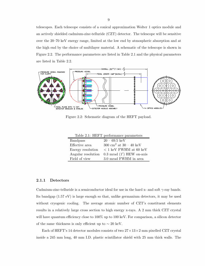
9

telescopes. Each telescope consists of a conical approximation Wolter 1 optics module and

an actively shielded cadmium-zinc-telluride (CZT) detector. The telescope will be sensitive

over the 20–70 keV energy range, limited at the low end by atmospheric absorption and at

the high end by the choice of multilayer material. A schematic of the telescope is shown in

Figure 2.2. The performance parameters are listed in Table 2.1 and the physical parameters

are listed in Table 2.2.

Figure 2.2: Schematic diagram of the HEFT payload.

Table 2.1: HEFT performance parametersBandpass 20 – 69.5 keVEffective area 300 cm2 at 30 – 40 keVEnergy resolution < 1 keV FWHM at 60 keVAngular resolution 0.3 mrad (1′) HEW on-axisField of view 3.0 mrad FWHM in area

2.1.1 Detectors

Cadmium-zinc-telluride is a semiconductor ideal for use in the hard x- and soft γ-ray bands.

Its bandgap (1.57 eV) is large enough so that, unlike germanium detectors, it may be used

without cryogenic cooling. The average atomic number of CZT’s constituent elements

results in a relatively large cross section to high energy x-rays. A 2 mm thick CZT crystal

will have quantum efficiency close to 100% up to 100 keV. For comparison, a silicon detector

of the same thickness is only efficient up to ∼ 20 keV.

Each of HEFT’s 14 detector modules consists of two 27×13×2 mm pixelled CZT crystal

inside a 245 mm long, 40 mm I.D. plastic scintillator shield with 25 mm thick walls. The

10

Table 2.2: HEFT physical parametersEnvelope 6.5 m long × 1 m dia.Telescope modules 14 co-alignedOptics

configuration conical approximation Wolter Ifocal length 6 mdimensions 4 – 12 cm radius, 40 cm lengthsubstrate thermally formed glasscoating materials W/Si

Detectorsmaterial CZTdimensions (2) 27× 13× 2 mm3

pixel pitch 0.05 cmshielding graded Z (passive) with plastic scintillator (active)

Mass 1270 kgPower consumption <300 W

plastic scintillator is used in anticoincidence with the detector to reduce background from

spallation products. The detector is further shielded from secondary x-rays by a series of

lead, tin and copper sleeves lining the inside wall of the plastic shield.

The pixel pitch of the detectors, 0.05 cm, oversamples the projected angular resolution

of the optics by a factor of 3. Each detector is indium bump-bonded to a VLSI chip with

separate event triggering, preamplification, and pulse sampling circuitry under each pixel.

This arrangement minimizes stray capacitance between the detector and the preamplifi-

cation stage, significantly reducing electronic noise in the detector electronics. The latest

tests of the detector/VLSI hybrid indicate that HEFT’s spectral resolution should fall in

the range 0.5 – 1.0 keV FWHM at 60 keV. For more details on the detectors see Harrison

et al. (2000) [26] and references therein.

2.1.2 Optics

The HEFT optics are configured in a conical approximation to the Wolter I geometry. In

the conical approximation, the half opening angle of the secondary mirror shell is three

times that of the primary shell. The half opening angle of the primary shell, α, is given by

4α = arctan(r/f) where r shell radius and f is the focal length as defined in Figure 4.1.

HEFT mirror shells are 40 cm long overall and range from 4 to 12 cm in radius. With its 6

11

m focal length, the primary opening angles will range from 1.67–5.0 mrad. Each telescope

module will consist of 72 nested mirror shells filling roughly 50% of the aperture. More

details on the shell packing arrangement and its optimization are discussed in Section 4.1.

The tight packing arrangement of HEFT’s optics requires that we use a mirror substrate

that is thin, stiff and light. The Wolter I geometry requires that the substrate be easily

formed into conical sections. Finally, in order to maximize the performance of the coatings,

the substrate must have relatively low (< 4A) surface roughness. D263, a borosilicate

glass produced by the DESAG division of Schott, meets the requirements for the HEFT

optics. D263 is manufactured in a “down-draw” process where the glass is formed by

flowing through a slot in the bottom of the melting tank. This manufacturing process can

produce glass in thickness ranging from 30–1100 µm with RMS surface roughness typically

less than 4 A. HEFT will use 200 and 300 µm thick D263, thermally formed [8] and then

cut into 10 cm long, 45 cylindrical sections. The glass is thin and flexible enough to allow

the mounting process to force the cylindrical glass sections into the conical configuration

required for focusing. X-ray reflectance tests comparing multilayer coatings on flat and

slumped glass showed that the slumping process did not adversely affect the surface quality

of the glass [7].

Two other common substrate materials for hard x-ray optics are epoxy-replicated alu-

minum foils (ERAFs) and electroformed nickel shells. We considered ERAFs for HEFT but

in the end decided that the production process would require too many sensitive steps and

that glass would provide equivalent to superior performance with much simpler production

methods. Electroformed nickel is attractive because it can be used to produce full-revolution

true Wolter I optics; however, it is prohibitively costly, requiring a separate mandrel for

each radius optic, and nickel shells would be much heavier than glass shells.

The main problem with glass as a substrate is its brittleness. A balloon payload must

be able to withstand shocks of 5–10 g that occur when the parachute opens during descent

and upon landing. Under such heavy loads, microscopic cracks in the edges of the glass

could propagate, shattering the optics. Standard mounting techniques, where the substrates

are bonded or clipped at their edges, would very likely break the glass substrates under

heavy loads. In order to mitigate this problem, we developed a mounting and assembly

method that would provide the optics with stable support and highly accurate alignment.

The mounting method, being executed by Colorado Precision Products, Inc. (CPPI), in

12

Boulder, CO, calls for the mirror segments to be bonded to precision machined graphite

rods. The rods are bonded along the entire length of the optics, parallel to the optical axis,

providing support for the glass. Segments are built up from the inner shell to the outer.

After a new set of rods are bonded to the back side of an optic, the rods are machined

to set the angle of the next optic. Because the angle machined into each rod is indicated

from the base of the segment, there is no buildup in mounting errors. Figure 2.3 illustrates

the mounting technique from an end-on view of the optics and shows a prototype using

uncoated glass on the assembly fixture at CPPI.

13

mandrel and machined.2. First glass optic is epoxied to the rods.

to the glass and machined.4. Next optic is epoxied to the rods.

1. Graphite rods are attached to the

3. Next set of graphite rods are attached

Alignment strongback

Graphite spacers

Figure 2.3: Top: The HEFT optic mounting and alignment procedure. Bottom: HEFTuncoated prototype optic on the mounting assembly fixture.

14

Chapter 3 Principles of x-ray multilayers

X-ray focusing can be achieved either through reflection or refraction. In the x-ray band,

the real part of the refractive index for all materials is less than the vacuum refractive

index by a very small amount (10−3–10−6 at 10 keV). Consequently, reflective optics must

operate at grazing incidence angles where a condition for total external reflection exists.

Refractive optics must use compound lenses to shorten the focal length to a usable distance

[27]. Refractive optics must have surfaces with small radius of curvature, so they are best

suited to situations where small apertures are acceptable. Also, because the refraction

angle, and hence the focal length, is energy dependent, refractive lenses are not suitable

for broad band applications. Grazing incidence reflective optics are the standard choice for

x-ray astronomy, where large apertures and energy independent focal length are important.

This chapter covers the basic physics of x-ray reflection from standard materials and

multilayer coatings. Multilayer coatings are considerably more complex than single-material

reflectors, so some multilayer design considerations and material selection criteria will also

be discussed.

3.1 X-ray reflection from standard materials

Standard materials, especially high Z elements, make highly efficient x-ray reflectors at

grazing incidence angles where a condition for total external reflection exists. Conversely,

at larger incidence angles, outside of the total external reflection regime, the reflectance

rapidly falls off to virtually unusable values. The energy dependence of the critical angle

for total external reflection limits the practical use of standard reflectors in astronomical

telescopes to low energies (E ∼< 15 keV).

The x-ray index of refraction, nr, of materials is often written as

nr = 1− Nreλ2

2π(f1 + if2) = 1− δ − iβ, (3.1)

where N is the number density of atoms, re is the classical electron radius, λ is the wave-

length of light, and f1 and f2 are atomic scattering form factors. The imaginary part of nr

15

is related to the absorption cross section (µa) and the transmission coefficient (T ) by the

following equations:

µa = 2reλf2 =4πβNλ

(3.2)

T (x) = exp(−Nµax). (3.3)

The real part of nr is used by Snell’s law to calculate the refraction angle. Because nr in

the x-rays is less than the refractive index in vacuum, x-rays exhibit total external reflection

at small grazing incidence angles. The maximum grazing incidence angle, or critical angle

(θc), is related to the refractive index by Snell’s law:

cos(θc) = nr. (3.4)

The relationship between photon energy and critical angle is found by combining Equations

3.1 and 3.4:

θc =√

2δ = λ

√Nref1

π. (3.5)

Since λ = hc/E, it is often stated that the critical angle is inversely proportional to the

incident photon energy. Although the form factor, f1, is also dependent on energy, its

dependence is weak. The form factor is the measure of the number of “free” electrons

in the system, i.e., the number of electrons whose binding energy is less than the photon

energy, so at energies greater than a few keV and away from photoelectric transitions, f1 is

nearly constant. In the following discussion, I will use the symbol ρe = Nf1 as the effective

electron density.

The reflectance function, R, of a standard (nonstratified) material is calculated from

the Fresnel formulae (see Born and Wolf 1980 for derivation):

rTE =sin θi − n sin θtsin θi + n sin θt

(3.6)

rTM =n sin θi − sin θtn sin θi + sin θt

, (3.7)

where n is the complex refractive index of the material, θi is the grazing incidence angle

(measured from the interface surface), and θt is the angle of the transmitted ray, which is

16

related to θi by Snell’s law. For unpolarized light, the reflectivity function is:

R =

∣∣∣∣∣rTE + rTM

2

∣∣∣∣∣2

. (3.8)

When θi < θc, the angle of transmission, θt, is imaginary, causing the terms in the numerator

of Equations 3.6 and 3.7 to be out of phase in the complex plane, resulting in Fresnel

coefficients with magnitude near 1. When θi > θc, then θt is real and because δ << 1,

θi ≈ θt, so the Fresnel coefficients are nearly zero. With the exception of Bragg reflection

off of crystalline solids, the x-ray reflectivity of standard materials is negligible at incidence

angles greater than the critical angle.

3.2 X-ray reflectivity from multilayers

In order to achieve appreciable x-ray reflectivity at incidence angles greater than θc, one

can use thin film coatings to create a synthetic Bragg crystal. Such thin film coatings are

commonly referred to as “multilayers” [4, 5]. In order to be effective at reflecting x-rays,

multilayers are deposited as alternating layers of high and low refractive index materials

(e.g., tungsten and silicon (W/Si), or platinum and carbon (Pt/C)). Figure 3.1 illustrates

a generic multilayer coating. Typical values for the layer thicknesses range from 10–100A

with total coating thicknesses up to a few microns.

The reflectance function of a multilayer coating can be calculated via recursive appli-

cation of the Fresnel formulae to the reflectivity calculation for a single film. The Fresnel

reflection coefficients for the jth interface are

rTEj =nj sin θj − nj+1 sin θj+1

nj sin θj + nj+1 sin θj+1(3.9)

rTMj =nj+1 sin θj − nj sin θj+1

nj+1 sin θj + nj sin θj+1, (3.10)

where nj is the complex refractive index of the jth layer. Snell’s law (nj cos θj = cos θi) is

used to calculate θj , the refracted angle of the transmitted beam. Because we are considering

grazing incidence angles, where cos θ ≈ 1, it is computationally more useful to use an

17

θj

parametersLayer Interface

parametersθij=0:

j=1:

j=2:

j-1:

j:

j+1:

j=2N-1:

j=2N:

σ

σ

σ

σ

σ

σ

σ

σ

0

1

2

j-1

j

j+1

2N-1

2N

2

j+1

j

j=2N: n t

j: n t

j+1: n t

j=2: n t

j=1: n t1 1

2

2N 2N

j+1

j

Substrate

Figure 3.1: Schematic diagram of a multilayer coating with notation corresponding to thatused in the text. Layers and interfaces are labeled by j, n is the complex index of refraction,t is the layer thickness, and σ is the interface width. Adapted from Joensen, 1995.

algebraically equivalent form of Snell’s law:

nj sin θj =√n2j + sin2 θi − 1. (3.11)

The reflectivity of the coating, R, is found by recursively calculating the reflection coefficient

for a single thin film:

r≥j =rj + r≥j+1 exp(−i2φj+1)1 + rjr≥j+1 exp(−i2φj+1)

, (3.12)

where r≥j is the combined reflection coefficient for interfaces j . . . 2N and φj is the change

in phase of the radiation as it passes through layer j with thickness tj:

φj =2πλtjnj sin θj. (3.13)

18

The recursion relation starts at the j = 2N th interface with r≥2N = r2N . It is safe to

assume that r2N+1, the reflection coefficient for the back side of the substrate, is zero as

long as the substrate is much thicker than the coating. The recursion ends at j = 0 and we

find the reflectivity of the coating:

R =| r≥0 |2 . (3.14)

The Fresnel formulae give us the reflectance function of a multilayer coating with perfect

interfaces. In practice, print-through of substrate roughness, deposited thin film roughness,

and interdiffusion between adjacent layers conspire to reduce reflectivity from the ideal case.

Roughness and interdiffusion are taken into account by multiplying the Fresnel coefficients

(r≥j) by the Nevot-Croce factor [28]:

FNC,j = exp

(−8π2

λ2(nj sin θj)(nj+1 sin θj+1)σ2

j

). (3.15)

The Nevot-Croce factor is essentially the Debye-Waller factor with refraction taken into

account.

3.3 General design considerations

3.3.1 Bilayer thickness range

The bilayer thickness, d, (or thicknesses, dk) of a multilayer coating is equivalent to the

lattice spacing of a crystal when one considers its Bragg reflection properties. The Bragg

formula, mλ = 2d sin θ (where m is an integer), is used to estimate (or calculate) the

bilayer thicknesses to be used in any particular application. For completeness, the refraction

corrected Bragg formula and its derivation are outlined here, but in practice, the standard

formula is used more often.

Multilayer coatings, like crystals, enhance reflectance via constructive interference be-

tween reflections from adjacent bilayers. Constructive interference is locally maximized

when the change of phase through a bilayer is and integer multiple of π, i.e., φj+φj+1 = mπ.

Using Equations 3.11 and 3.13 and assuming that β δ 1 and θc < θi 1, one can

19

derive the refraction-corrected Bragg formula [29]:

mλ = 2d sin θ

√1− 2(Γjδj + Γj+1δj+1)

sin2 θ, (3.16)

where m is the order of the reflection, d is the bilayer thickness and Γj = tj/d.

By inverting the first-order (m = 1) Bragg equation for d, one can estimate the range in

bilayer thicknesses required to enhance reflectance over the energy range Emin − Emax and

angular range θmin − θmax:

dmin =hc

2Emax sin(θmax)

(1− 2(Γ1δ1 + Γ2δ2)

sin2 θmax

)−1/2

(3.17)

dmax =hc

2Emin sin(θmin)

(1− 2(Γ1δ1 + Γ2δ2)

sin2 θmin

)−1/2

. (3.18)

For the minimum bilayer thickness, we can drop the refraction-correction term because

typically θmax θc. The maximum bilayer thickness, however, requires more careful atten-

tion because specifications (including those for HEFT) may result in a substantial refraction

correction. When θmin ≈ θc, the standard Bragg formula for crystals underestimates the

maximum bilayer thickness.

3.3.2 Bilayer thickness distribution

Broadband reflectivity is achieved with multilayer coatings by varying the bilayer thick-

nesses throughout the coating. Lateral gradations are used in some specialized thermal

neutron beam or synchrotron applications, but for astronomical x-ray telescopes, depth

graded multilayer coatings are the norm. The Bragg formulas, Equations 3.17 and 3.18,

give the required range in bilayer thicknesses for a given application, but the distribution of

bilayer thicknesses still must be specified. Methods for specifying the bilayer thickness dis-

tribution generally fall into two categories: power-law distributions and “needle variation”

derived distributions.

Power law distributions are motivated by the fact that more bilayers are needed to

achieve a given level of reflectance for high energy photons than are needed for low energy

photons. The Fresnel reflection coefficients, Equations 3.9 and 3.10, show that r ∝ δj−δj+1

(assuming β δ 1 and θc < θi 1). Since δ ∝ ρe/E2, we find that the reflection

20

coefficients scale as ∆ρe/E2. Ignoring attenuation and scattering due to roughness, this

implies that each factor of 2 in energy requires 24 times as many bilayers in order to achieve

a flat response.

The use of power-law bilayer thickness distributions originated with F. Mezei (1976)

[30], who was also the first to propose the use of multilayer coatings for the reflection of

thermal neutrons. Mezei’s approach to power-law parameterization is outlined in Joensen

(1995) [31] and will not be repeated here. Mezei (1976) derives a power-law formula for flat

response, broadband neutron mirrors assuming that N , the number of bilayers, is large and

ignoring multiple reflections and absorption/extinction. The Mezei formula is

d(k) = dc/k0.25, (3.19)

where k is the index of the bilayer consisting of layers j = 2k − 1 and j = 2k, and dc =

λ/2 sin θc. Note also that his definition for the maximum bilayer thickness (dc) does not

include any refraction corrections to the Bragg formula.

Other power-law parameterizations have been developed [32, 33, 34] but will not be

expanded upon, with the exception of Joensen’s parameterization. In his thesis, Joensen

proposes an empirical distribution formula which is a generalization of the Mezei formula:

d(k) =a

(b+ k)c(3.20)

with a, c > 0 and b > −1. Using the energy weighted average reflectance at a single incidence

angle as his figure of merit, Joensen finds superior performance with his parameterization

when compared against those of Mezei (1976), Schelten and Mika (1978), Hayter and Mook

(1989), and Yamada et al. (1978). For this reason, Joensen’s parameterization is used in

the optimization of the HEFT multilayer design.

The other major class of multilayer designs involves the needle variation technique,

where a merit function is used to predict locations in the coating design where the addition

or subtraction of bilayers will improve the desired reflectance response. This technique was

pioneered in the 1980s by Tikhonravov (1982) [35] and Baskakov (1984) [36]. The needle

variation method is potentially very useful for solving the inverse of the Fresnel formulae,

i.e., calculating a bilayer distribution from a desired reflectance profile. For example, in the

21

work of Kozhevnikov et al. (1998, 2001) [37, 38], a recursion relation has been developed

to calculate an initial distribution for a given reflectance profile. Standard minimization

techniques (Newton-Raphson, Levenberg-Marquadt, simplex) are then used to minimize

the mean square difference between the calculated reflectance and the desired profile. The

limitation to Kozhevnikov’s present method is that the number of bilayers is fixed, narrowing

the search space considerably, but also, very likely, missing the true optimal design. It is

possible that the needle variation technique, in conjunction with Kozhevnikov’s recursion

relation, would be a very powerful technique for solving the “inverse problem.”

3.4 Multilayer materials

In choosing material combinations for a graded multilayer one must consider that the band-

pass and the reflectivity are limited by attenuation in the multilayer coating because of

photoelectric absorption and scattering at the interfaces. The ideal material pairs have a

large difference in refractive index; minimal absorption over the energy range of interest;

and can be fabricated with sharp, smooth interfaces.

The Fresnel formulae (Equations 3.9 and 3.10) show that the reflectance of an interface

scales with the difference in refractive index between the two sides of the interface. As

previously discussed, δ ∝ ρe and since the effective electron density is proportional to

the mass density, one can use bulk density as an initial screen to find promising pairs of

materials for multilayers. At the energies of interest (10-100 keV), photoelectric absorption

is the main component of an atom’s cross section and, away from absorption edges, it scales

roughly as Z4E−5/2. Highly absorbing materials are to be avoided because the reflectance

of a multilayer made with such materials levels off with fewer bilayers than that of a coating

using smaller cross section materials. Thus, if the reflectivity per interface is the same, the

material combination with a lower absorption coefficient will have better reflectance.

Photoelectric absorption edges must also be considered when choosing materials. For

example, at the W K-absorption edge (69.5 keV), the reflectivity of a W/Si graded multilayer

drops considerably, as shown in Fig. 3.2. The reflectivity of a Cu/Si multilayer with the

exact same specifications, shown as the dotted curve in Fig. 3.2 demonstrates that the cutoff

is not due to the multilayer’s bilayer distribution. A broadband reflector that uses tungsten

is therefore limited either to energies below the W K-edge or significantly above it.

22

Figure 3.2: Calculated reflectivity vs. photon energy at 1.75 mrad of a graded W/Si mul-tilayer and a Cu/Si multilayer with the exact same specifications (bilayer thickness distri-bution and interface width). The Cu/Si reflectivity demonstrates that the range in bilayerthicknesses for this mirror would allow reflectivity at 1.75 milliradian from 20 to 100 keV,but the jump in absorption at the W K-edge (69.5 keV) drastically reduces reflectivity ofthe W/Si multilayer above the absorption edge.

Following the selection of materials based on refractive index contrast and minimal ab-

sorption, one must experimentally determine which material combinations are compatible.

Problems that may arise include excessive interdiffusion, which reduces the refractive index

contrast, high levels of stress in the film, which may result in delamination, and corrosion.

Other experimentally determined factors include maximum deposition rates of the materials

and deposited surface roughness.

The most common high-density materials in x-ray multilayers are Pt, W, Ni, and Mo.

The most common low density materials are C, B4C, and Si. The HEFT project will use

primarily W/Si since this combination has been found to produce stable coatings with

relatively low (σ = 3.5A) roughness interfaces.

23

Table 3.1: Comparison of the physical properties of a few multilayer material combinations[2]. Absorption coefficients are given for 30 keV x-rays.

materials ρ1/ρ2 µ11 µ2

2

[cm−1] [cm−1]Pt/C 9.77 566. 0.435W/Si 8.28 439. 3.35Mo/Si 4.38 287. 3.35Ni/C 4.05 92.0 0.435Cu/Si 3.85 97.8 3.35

24

Chapter 4 Optimization of multilayer designs

The current literature on multilayer optimization almost exclusively deals with maximizing

integrated reflectance [39, 40] or matching the reflectance to a desired function [39, 37, 41]

either over a range of photon energies at a single reflection angle or over a range or reflection

angles at a single photon energy. Optimization methods that optimize a multilayer design

for a single angle or a single photon energy may be useful for laboratory applications where

reflection angles and/or photon energies are fixed. For a general-purpose astronomical hard

x-ray telescope, however, maximizing the effective area over a given energy range and field

of view (i.e., a relatively wide range of incidence angles) is more important than producing

a specific response at a single energy or reflection angle. For example, galaxy clusters

and nearby radio galaxies are extended at the few arcminute level. In addition, for a

balloon-borne instrument, one must account for instabilities in the pointing of the telescope

which can also be at the few arcminute level. For these reasons, the off-axis performance

of astronomical x-ray telescopes deserves at least as much attention as the often-quoted

on-axis performance.

To this end, I devised a figure of merit function that is the field-of-view and energy-

weighted average effective area of a telescope’s optics [42]. The calculation of the figure

of merit requires specification of the geometry of the telescope optics, weighting functions

for spectral and angular response and the matrix of multilayer reflectivity vs. energy and

incidence angle.

4.1 Geometry of the optics

The first step in multilayer optimization is specification of the geometry of the telescope’s

optics. Off-axis performance is strongly affected by vignetting, so the optimum geometry is

determined by balancing on-axis collecting area with off-axis vignetting. The geometry is

also crucial to the multilayer design optimization because the reflection angle distribution

on each mirror is needed to calculate the throughput of the optics. For both tasks, one runs

a Monte Carlo ray trace using roughly 108 input events. The off-axis angle distribution

25

used in the ray trace affects the optimization of the geometry of the optics and determines

the reflection angle distributions that will be used to calculate the figure of merit. I use a

uniform distribution of off-axis angles between 0 and 3 mrad, with the largest angle set by

the size of our detectors and the focal length of the telescope. To design geometries and

multilayers with greater off-axis performance (at the expense of on-axis performance), one

would use an input distribution that favors off-axis photons.

HEFT’s optics are arranged in a conical approximation to the Wolter I (parabola/

hyperbola) geometry. HEFT uses thermally slumped glass which presently has figure errors

that result in a point spread function at the 1′ level. A schematic of the optics’ geometry

and the relevant angles are shown in Figure 4.1. The half-opening angles of the mirror shells

are set by the following equations:

αi = ri/(4f) (4.1)

βi = 3αi, (4.2)

where αi and βi are the respective half-opening angles of the primary and secondary shells,

ri is the radius of the ith shell at the plane between the primary and secondary mirror

sections (4–12 cm for HEFT), and f is the focal length of the telescope (6 m for HEFT).

The HEFT substrates are 0.3 mm thick, 20 cm long sheets of Schott DESAG D263 glass.

The difference in radii between consecutive concentric mirror shells produces a tradeoff

between on- and off-axis collecting areas. On-axis collecting area is maximized when the

inner radius of the i+ 1st primary shell lies on the same coaxial cylinder as the outer edge

of the ith primary shell. Increasing the radial gap (cf Figure 4.1) between consecutive shells

improves off-axis collecting area at the expense of on- and nearly on-axis area. I explored

two methods of defining the extra gap between mirror shells: a constant gap between all

shells, such that the difference in radii between consecutive shells is

∆ri,i+1 = αil + const., (4.3)

where l is the length of the mirror along the optical axis, and a radius dependent gap where

the gap between the consecutive shells is

∆ri,i+1 = αil + ξαil, (4.4)

26

i + 2

i + 1

ri

fi+1

i+1

i+1

radial gap

off-axis rayon-axis ray

optic

al a

xis

to focal plane

Figure 4.1: Geometry of conical-approximation Wolter I optics with primary and secondaryreflection angles for on- and off-axis rays.

where ξ is the variable gap parameter. When ξ = 0, there is no additional gap between

shells; when ξ = 1, the gap is equal to the projected radial width of the primary shell. From

ray tracing with perfect reflectivity, R = 1, one finds that the angularly averaged collecting

area (the fraction of collected events multiplied by the illuminated area) is maximized with

a constant gap of 0.17 mm between consecutive shells (see Figure 4.2). A variable gap with

ξ = 0.26 maximizes the area for that method, but falls short of the constant gap geometry

by a fraction of a percent.

4.2 Effective areas

The effective are of an optical system is the product of the physical collecting area, the

reflectance of the mirrors, and transmission functions of windows, covers, and the ambient

medium. Section 4.2.1 covers the geometry-dependent aspects of the effective area, and

section 4.2.2 covers transmission corrections to the geometric area.

27

Figure 4.2: Angularly averaged collecting area vs. radial gap between mirror shells. Variablegap results (+) are plotted against the bottom scale and constant gap results (×) areplotted against the top scale. Each area is determined by ray tracing 108 events uniformlydistributed in off-axis angles between 0 and 3 mrad, and uniformly distributed spatiallyover the 12 cm radius aperture. The standard deviation in the estimate of the area is 0.025cm2.

4.2.1 Geometry-dependent area

The physical collecting area and the mirror reflectance function are the the two components

of the geometry-dependent part of the effective area. On-axis effective area is easy to

calculate, since the incidence angles on the primary and secondary mirrors are identical.

The area of the ith shell is thus

Ai(E) = (2πriαil) · ([R(E,αi)]2), (4.5)

where l is the length of the mirror along the optical axis and E is the energy of the photon.

The first term in the above equation is the projected area of the primary mirror, and the

second term gives the reflection efficiency.

Off-axis effective areas are more complicated to calculate because the incidence angles on

the two mirrors differ for off-axis photons. Calculation of the off-axis effective area requires

knowledge of the incidence angle distribution on each mirror. Consider photons arriving

28

from a source at off-axis angle ψ. The incidence angles on the primary and secondary mirrors

are θ1 = α + ψ1 and θ2 = α+ ψ2, respectively. The angles ψ1 and ψ2 have values between

−ψ and ψ, depending on the difference between the azimuthal angle of the source and the

azimuthal position of the point of reflection, ∆φ. For example, when ∆φ = 0, ψ1 = −ψ

and when ∆φ = π, ψ1 = ψ. With conical approximation Wolter I optics with α 1, one

can make the approximation that ψ1 = −ψ2. This approximation allows one to calculate

the effective area using only the incidence angle distribution on the primary mirrors. The

one-dimensional function Winc(αi, ψ1) is the incidence angle distribution generated by the

ray trace with off-axis angles uniformly distributed between 0 and 3 mrad. Winc has units

of area and is related to the event distribution (the raw output of the ray trace) by the

density (events/unit area) of input events. The angularly weighted effective area is

Ai(E) =∫ ψ

−ψdψ1Winc(αi, ψ1) · [R(E,αi + ψ1)R(E,αi − ψ1)] (4.6)

where ψ is the half angle of the full field of view. There is no explicit integration in

the azimuthal (φ) direction in Equation 4.6 because it is already incorporated into the

distribution function by the ray trace.

If one cannot use the approximation ψ1 = −ψ2, then it is necessary to explicitly

keep track of the correlation between ψ1 and ψ2 in the ray trace and generate a two-

dimensional incidence angle distribution for each set of mirror shells. A contour map of the

two-dimensional incidence angle distribution for HEFT’s the outermost set of mirrors and

associated projections are shown in Figure 4.3. The sum of the deviation angles, ψ1 +ψ2, is

used instead of ψ2 alone on the y-axis and the contours denote logarithmic intervals. The

Figure 4.3 demonstrates the excellent degree to which the ψ1 = −ψ2 approximation is valid

for conical approximation Wolter I optics. Note that the y axis scale is in microradians,

whereas the x axis scale is in milliradians. With a two-dimensional distribution, the angu-

larly weighted effective area is

Ai(E) =∫ ψ

−ψdψ1

∫ ψ

−ψdψ2Winc(αi, ψ1, ψ2) · [R(E,αi + ψ1)R(E,αi + ψ2)]. (4.7)

Use of the exact formula for the area allows application of this technique to other reflection

geometries such as Kirkpatrick-Baez or a true parabola/hyperbola Wolter I. In addition,

29

extending the technique to geometries with even more reflections is trivial: one simply adds

one dimension to the incidence angle distribution matrix for each additional reflection.

Figure 4.3: Upper left: The two-dimensional reflection angle distribution, Winc(α =5 mrad, ψ1, ψ2). Because the distribution is nonzero only near the line ψ1 = −ψ2, it ismapped as ψ1 + ψ2 vs. ψ1. Each contour line demarcates a factor of ten in the magnitudeof the weighting function. Upper right: Projection of the distribution onto the ψ1 + ψ2

axis. One half of the distribution lies within 0.625 µrad of ψ1 + ψ2 = 0 and 90% of thedistribution lies with 7.5 µrad. Lower left: Projection of the distribution onto the ψ1 axis,Winc(α = 5 mrad, ψ1).

4.2.2 Transmission components of the effective area

In addition to the geometry-dependent parts of the effective area, it is important to take

into account known absorbers between the source and the detector and the detector’s quan-

tum efficiency (QE). In the case of HEFT, where we have a balloon-borne telescope, the

absorbers include mylar windows to protect the optics, a kevlar pressure vessel that houses

30

the detectors, and, most importantly, the atmosphere above the telescope. HEFT uses CZT

detectors and in the energy range of interest, the QE of CZT is not a strong function of

photon energy.

The transmission function for atmospheric attenuation is defined as

Tatm(E, ρatm) = exp(−η(E)ρatm), (4.8)

where η(E) is the attenuation coefficient of dry air and ρatm is the altitude dependent

atmospheric column density. The area is thus redefined:

A(E, ρatm) = A(E)Tatm(E, ρatm). (4.9)

For HEFT, we assume a column density of 3.5 g/cm2, corresponding to an altitude of 39

km.

At this time the thicknesses of the kevlar pressure vessel and the mylar windows on the

mirrors have not been decided upon; however, the transmission functions of these windows

are expected to be close to unity at energies above 20 keV. Consequently, their omission

will not significantly change the results of the optimization.

4.3 Figure of merit function

We use the angularly weighted effective area to calculate the figure of merit (FOM) for

specific multilayer bilayer distributions. In the FOM we include an additional, energy-

dependent weighting function, WE(E), that allows flexibility in defining the spectral re-

sponse of an optimized design. We use an energy weighting function that increases with

energy because almost all astronomical sources have falling x-ray spectra. The energy

weighting function is normalized so that its integral over the energy range of interest is

unity. The FOM is thus the weighted energy integral of the field-of-view averaged effective

area for each mirror shell, summed over all mirrors:

FOM =∑Ni=1

∫ EmaxEmin

dEAi(E)WE(E)Emax − Emin

. (4.10)

The advantages of using Equation 4.10 as a figure of merit are as follows: (1) it takes

31

into account the performance across the field of view, (2) it can be used to compare different

telescope designs (given the same weighting functions), and (3) it allows us to automate the

optimization of multilayer designs for a given optics geometry.

4.4 Design optimization

4.4.1 Parameterization of the bilayer distribution

Optimizing an unconstrained multilayer design is extremely computationally intensive be-

cause of the size of the parameter space that must be searched. When the materials are

selected ahead of time, a multilayer design with N bilayers has 2N free parameters. If one

ignores the realities of thin film deposition (finite targets, internal film stresses, interfacial

roughness), any measure of the average reflectance will improve with increasing coating

thickness, tcoating. One may reasonably assume that the improvement will be negligible

when the minimum distance traveled through the coating (∼ 2tcoating/ sin θmax) is a few

times the mean free path of photons with energy Emax1, but the difficulty of the problem

is still compounded by the fact the N is not known a priori.

The problem of optimization is greatly simplified if one parameterizes the layer thickness

distribution. Parameterization greatly reduces the search space, but there is always the

concern that it may exclude globally near-optimal solutions. The work of Kozhevnikov et al.

[37], who use a recursion relation to establish an initial guess, and Michette and Wang [39],

who start their optimization with Joensen’s power-law parameterization (Equation 3.20),

demonstrate that power-law and recursion relation parameterizations will give solutions that

are globally near-optimal for wide bandpass applications such as astronomical telescopes.

Using Joensen’s parameterization, the bilayer thickness distribution can be specified

with the four parameters a, b, c and N . It is, however, more convenient to specify dmin =

d(N), dmax = d(1), c, and N because it is easier to understand the physical effects of dmin

and dmax than the effects of a and b on reflectance. Since Joensen’s parameterization only

specifies the bilayer thickness distribution, one must also specify the fractional thickness of

the high Z layer within each bilayer (Γk). A Joensen-parameterized graded multilayer is

thus specified with N + 4 parameters. One may further reduce the number of adjustable1The mean free path of a 69 keV photon in tungsten is 5.8 mm. The maximum incidence angle for HEFT

is 8 mrad. Thus, even an idealized mirror coating should not contain more than 23 µm of tungsten.

32

parameters by restricting designs to those with a single value of Γ, cutting the number of

parameters from N + 4 to just five: N , c, Γ, dmin and dmax.

4.4.2 Bilayer thickness range

The refraction-corrected Bragg formulae (Equations 3.17 and 3.18) define the relationship

between bandpass (Emin . . . Emax), angular acceptance range (θmin . . . θmax), and bilayer

thickness range. The angular acceptance range for a set of conical approximation Wolter

I mirrors with primary half-opening angle α and field of view 2Ψ is given by the following

equations:

θmin =

α−Ψ α−Ψ > θc

θc α−Ψ < θc(4.11)

θmax =

α+ Ψ Ψ < α

2α Ψ > α(4.12)

where θc is the critical angle for total external reflection (√

2δ for a pure material,√

2(Γ1δ1 + Γ2δ2)

for a 2 component multilayer). At angles less than θmin, the photon is either out of the

field of view (θ < α − Ψ) or in an angular range where it will reflect by total external

reflection (θ < θc). At angles greater than θmax, the photon is either out of the field of

view (θ > α+ Ψ) or striking the primary mirror at an angle where it will not reflect off the

secondary mirror and will not hit the focal spot (θ > 2α). The resulting values of dmin and

dmax theoretically cover the entire range required for first order reflection.

In practice, Equations 3.17, 3.18, 4.11, and 4.12 only serve as guidelines for calculating

the bilayer thickness range. For different reasons, one is forced to adjust both the maximum

and minimum bilayer thicknesses from their calculated values.

In the case of dmax, we know from the diffraction corrected Bragg equation that the un-

corrected Bragg equation underestimates the bilayer thickness when θ ≈ θc. Using Equation

3.18, by the definition of θc, dmax → ∞ as θ → θc. Physically, when θ ≈ θc, the refracted

beam travels nearly parallel to the plane of the interface, thus requiring ever increasing

film thickness in order to reflect off the back surface. For broad bandwidth applications,

where power-law distributions are applicable, the bilayer thicknesses drop very quickly from

dmax. The implications are twofold: first, the total coating thickness is not a strong function

of dmax, second, the interference peaks from the top-most layers are relatively broad, i.e.,

33

∆θ ≈ θi/m, where m represents the number of participating interfaces2. Because fewer

bilayers are needed at low energies and because the resulting interference peaks are broad,

the figure of merit is not expected to be a strong function of dmax. Thus, in cases where

θmin = θc, one uses the uncorrected Bragg equation to define a lower limit to dmax but

in practice uses a larger value in order to smooth the transition between total external

reflection and multilayer reflection.

In the case of dmin, it can be difficult or impractical to fabricate the calculated minimum

bilayer thicknesses or the calculated value would result in an optimized coating that is

unrealistically thick. Bilayers with thickness less than 10A are difficult to reliably deposit

with present technology, and the typical interface widths (from interdiffusion and interfacial

roughness) would be a large fraction of the bilayer thickness. It is often necessary to use

a minimum bilayer thickness greater than the thickness specified by Equations 3.17 and

4.12. Raising dmin reduces the bandpass of the optics, affecting the high-energy response

at large reflection angles (at the edges of the field of view). The reduced bandpass that

comes with raising dmin also results in a much smaller optimized total coating thickness.

Fortunately, the desirable effect of reducing optimized coating thickness is strong because

of the power-law parameterization and the reduction in the figure of merit is small.

The effect of raising dmin on the figure of merit is small because events with large

reflection angles comprise a very small fraction of the total number of accepted events.

The angular weighting function, shown in Figure 4.3 for the outermost set of mirror shells,

approaches zero at extreme values of ψ; therefore, the contribution to the figure of merit

also approaches zero. Another way to look at the effect of dmin on reflectance is to consider

the effect of changing dmin on the effective area for a point source at off-axis angle ψsrc.

The minimum bilayer thickness affects the reflectivity of the outermost set of shells to the

highest energy photons from a source at the edge of the field of view (ψsrc = Ψ). The

incidence angle distribution is nearly uniform between α− ψsrc and α+ ψsrc. Raising dmin

by reducing the maximum reflection angle from θmax to θ′max thus reduces the effective area

(at energy Emax) presented to a source at the edge of the field of view roughly by a factor

of θmax−θ′maxΨ .

The bilayer thickness ranges actually used in the HEFT design and the methods for2Given m sources in a line separated by distance d and assuming θ 1, one find that the first order

interference peak falls to zero at λ/(md).

34

determining them are discussed in Section 4.5.

4.4.3 Optimization algorithm, characteristics of the FOM surface

Joensen’s power-law parameterization of the bilayer thickness distribution reduces the op-

timization phase space from 2N parameters down to 5: N (number of bilayers), c (power

law index), Γ (fractional thickness of the high Z material), dmin and dmax. Although the

optimization will not find the asymptotic figure of merit, one may be confident, given the

results of Kozhevnikov and Michette, that the result will be close. The goal of this opti-

mization scheme is not merely to find the set of parameters that maximizes the figure of

merit, but also to find the functional dependence of the figure of merit vs. coating thickness.

Having this information in hand allows one to quickly make tradeoffs between overall coat-

ing performance and fabrication time. By shrewdly choosing dmin and dmax based on the

arguments presented in the Section 4.4.2, the optimization is reduced to three parameters

and the thickness is controlled largely by N .

The optimization problem is reduced to finding optimal values of c and Γ for several

values of N . This two-dimensional optimization is efficiently carried out using the amoeba

algorithm from Numerical Recipes [43], which is based on the downhill simplex method

of Nelder and Mead [44]. Downhill simplex works well in this restricted parameter space

because the figure of merit surface does not exhibit local extrema over a wide range of

parameter space near the (restricted) absolute optimum. Figure 4.4 shows the contour

map of a c, Γ figure of merit surface at two values of N . In the figure, the dotted lines

depict an N = 200 surface and the solid lines represent an N = 250 surface. In addition to

demonstrating the regularity of the figure of merit surface, the figure also shows that the

figure of merit is much more sensitive to changes in c than Γ and that the optimum values

for c and Γ decrease with increasing N .

In the optimization program used for HEFT, one starts with a value of N that is

known by experience to be well below the optimal value and upon completion of each

(c,Γ) optimization, N is incremented by a factor of 1.25. The process is repeated until

the optimum figure of merit for successive values of N decreases3. The optimization is3Recall that at some point the figure of merit decreases with increasing N only because the parameter-

ization restricts the space of allowable bilayer distributions. In a global optimization, the figure of meritwould asymptote or plateau at some value that depends on the properties of the materials and the interfacialroughnesses.

35

Figure 4.4: Figure of merit contour maps of a Joensen parameterized graded multilayer.The dotted lines represent an N = 200 surface and the solid lines represent an N = 250surface. The calculations were performed for HEFT’s innermost set of mirror shells.

robust with respect to initial values of c and Γ because of the regularity of the figure of

merit surface. The optimization at each subsequent value of N starts with the optimal

parameters from the previous step. The optimization terminates at each value of N when

the range of figures of merit at the vertices of the simplex are fractionally less than 0.003.

With this criteria, c and Γ are typically optimized in 10–30 steps.

For each set of parameters, the reflectance matrix must be entirely recalculated. A

modern desktop computer will calculate a single reflectance matrix (∼ 8× 105 elements) in

3–10 minutes, depending linearly on the number of bilayers. Fortunately, the calculation of

reflectance matrices lends itself well to parallelization because the calculation time for any

element of a given matrix is the same and does not depend on other elements in the matrix.

With parallel processing, the time to calculate the figure of merit for a given parameter

set scales as 1/(number of processors). With the 32 and 64 processor systems available

through Caltech’s Center for Advanced Computing Research, the time required to optimize

the HEFT design was reduced from weeks to hours.

36

4.5 The HEFT optimization

The optimization process is best illustrated by describing its application to HEFT. The

specifications for HEFT that relate to multilayer design will be repeated here. After the

angular and energy ranges are defined, the Bragg equation is used to determine the bilayer

thickness range. As discussed above, one generally uses a bilayer thickness range narrower

than what one would calculate from Equations 3.17, 3.18, 4.11, and 4.12. The final product

of the optimization is a discretized curve of figure or merit vs. coating thickness with the

optimal parameters (N, c,Γ) at each step.

The geometry of HEFT’s optics and the dimensions of its detectors define field of view

and thus the range of possible reflection angles. HEFT is a 6 m focal length balloon-borne

hard x-ray telescope consisting of 14 identical co-aligned telescope modules. In each module,

there are 71 mirror shells between 4 and 12 cm radius (half opening angles 1.67–5.0 mrad)

configured in a conical-approximation Wolter I geometry. The detector is a 25 × 25 mm

pixelled CZT detector, allowing a maximum off-axis angle of 3 mrad at the corners. As

described in Section 4.2.1, the angular weighting function is generated by ray trace, with

the off-axis angle of the input photons uniformly distributed between 0 and 3 mrad.

Atmospheric absorption and the choice of multilayer materials set HEFT’s bandpass

to 20–70 keV. The low end of the energy range is limited by atmospheric absorption. At

a float altitude of 39 km, there is 3.5 g/cm2 of air between the source and the detector

giving a transmission function of 0.54 at 70 keV, 0.29 at 30 keV and 0.07 at 20 keV. The

high end of the energy range is set by the tungsten K absorption edge (69.5 keV). The

material combination W/Si was chosen because of the small interface widths (σ = 3.0− 3.5

A) achievable with this combination and because both components can be deposited at

high rates (∼> 1 A/s). The energy weighting function, WE, is proportional to E[keV] + 70,

giving the highest energy photons roughly 1.5 times the weight of the lowest energy photons.

The gradually rising linear function pushes the optimization towards designs with flatter

response. As discussed in Section 3.3.2, the Fresnel reflection coefficients scale as ∆ρe/E2;

without a rising weighting function, an optimization would boost low energy response at the

expense of high energy response. Admittedly, the choice of WE here is somewhat arbitrary

and one may find other functional forms that would be appropriate for other applications.

The bilayer thickness range can be defined for each pair of mirror shells or it can be

37

defined for a group of shells. From a fabrication point of view, it is no more difficult to coat

the same design on all mirrors or to coat a different design on each mirror. The main con-

straints in fabrication are the minimum layer thickness and the maximum coating thickness.

The minimum layer thickness depends on the properties of the material combination and

the maximum coating thickness depends on the stability of the coating chamber and the

production schedule. From a computational point of view, designing for groups of mirror

shells is more practical. Alternate telescope specifications often need to be investigated and

a quick mirror design turnaround make for efficient evaluation of the alternate specifica-

tions. HEFT mirror shells are divided into 10 logarithmically spaced groups, reducing the

range of mirror shell opening angles within each group from 3 to 10√

3 ≈ 1.12.

Table 4.1 summarizes the minimum and maximum bilayer thickness specifications for

each of HEFT’s mirror groups. As described in Section 3.3.2, coating thickness is a strong

function of dmin, whereas figure of merit is a weak function of dmin. Specifications for dmin

are increased from their calculated values so that the thickness of optimized designs falls in

the range 1.0–1.5 µm, dictated by the HEFT production schedule. An absolute minimum

bilayer thickness of 23A (for W/Si) is also imposed on the design due to limitations in

thin film deposition technology. Although thinner W/Si bilayers have been demonstrated

[45], the coatings do not perform well when the layer thicknesses become comparable to the

interface widths, σ ≈ 3.5A for W/Si. Specifying an absolute minimum thickness guarantees

that the minimum single layer thickness is always greater than 2σ. On the outer three

groups of mirror shells, the minimum bilayer thickness reduces the on-axis bandpass below

Table 4.1: HEFT design: mirror groups and bilayer thickness specifications.

mirror angular range radial range shells per dmin dmax

group [mrad] [cm] module [A] [A]1 1.67-1.86 4.00-4.46 6 33.3 297.62 1.86-2.08 4.46-4.99 6 29.9 266.63 2.08-2.32 4.99-5.57 7 28.7 238.94 2.32-2.59 5.57-6.22 7 27.4 214.05 2.59-2.89 6.22-6.94 7 26.1 191.86 2.89-3.22 6.94-7.73 7 24.7 171.87 3.22-3.60 7.73-8.64 7 24.6 153.98 3.60-4.01 8.64-9.62 8 24.3 137.99 4.01-4.48 9.62-10.75 8 23.7 123.610 4.48-5.00 10.75-12.0 8 23.0 110.7

38

70 keV. The effects of raising dmin on high energy and large angle reflectivity are summarized

in Table 4.2.

Unlike dmin, dmax does not strongly affect the total coating thickness. Even so, in cases

where θmin as calculated by Equation 4.11 is close to θc, the refraction corrected Bragg

formula (Eqn. 3.18 specifies an unreasonably large bilayer thickness). Experience has shown

that using the standard (uncorrected) Bragg formula with θmin = αmin/1.6, where αmin is

the half-opening angle of the group’s innermost shell, results in a reflectance profile that

smoothly transitions between total external reflection and interference enhanced reflection.

With the field of view and angular range, energy bandpass, mirror groupings, and bilayer

thickness range all settled, we are almost ready to determine optimum values of N ,c, and Γ

for each of HEFT’s mirror groups. The remaining inputs are airmass (3.5 g/cm2 for flight

at 39 km), interfacial width/roughness (σ = 3.5 A), and mass density of the deposited

materials (I assume bulk density in the absence of better information).

Table 4.2: Comparison of multilayer performance limits (idealized case vs. HEFT parame-ters). Column 3 (θmax): maximum reflection angle at the maximum photon energy. Column4 (Emax): maximum on-axis reflected energy on the outermost shell within each group, dis-regarding absorption edge effects. Column 5: estimated fractional loss in 70 keV effectiveeffective area for sources at the edge of the field of view.

(via Eqn 4.12) / (adjusted)mirror dmin θmax [mrad] Emax [keV] ∆θmax/Ψgroup [A] (E = 70 keV) (θ = αmax) (E = 70 keV)

1 23.8 / 33.3 3.72 / 2.66 140 / 100.1 0.572 21.3 / 29.9 4.16 / 2.96 140 / 99.9 0.573 19.1 / 28.7 4.64 / 3.09 140 / 93.2 0.674 17.1 / 27.4 5.18 / 3.23 140 / 87.5 0.755 15.3 / 26.1 5.78 / 3.39 140 / 82.3 0.826 14.2 / 24.7 6.22 / 3.59 135 / 77.9 0.887 13.4 / 24.6 6.60 / 3.60 128 / 70.1 1.008 12.6 / 24.3 7.01 / 3.64 122 / 63.6 N/A9 11.8 / 23.7 7.48 / 3.74 117 / 58.4 N/A10 11.1 / 23.0 8.00 / 3.85 112 / 53.9 N/A

4.5.1 Results of the optimization for HEFT

The final product of the optimization is a locus of points tracing out the figure of merit vs.

N . Analysis of the results from mirror group 4 are presented in this section. Results for

39

the full HEFT design are detailed in Appendix A.

Figure 4.5 shows the results of the mirror group 4 optimization. The optimization was

started with N = 150. After each optimization of c and Γ, N is increased by a factor of 1.25

and the (c,Γ) optimization is run again. The program terminates when the figure of merit

decreases with an increase in N . In this case, the figure of merit falls off after N = 363

with a corresponding coating thickness of 1.27 µm. For HEFT, we use this information to

trade 2% of the figure of merit for a substantially thinner coating. The N = 233 design

has roughly 98% of the area of the optimum design but its coating thickness is 30% thinner

than the N = 363 design’s coating.

Figure 4.5: Figure of merit vs. coating thickness for HEFT’s α = 2.32–2.59 mrad mirrors.The dashed lines indicate levels of 98% and 95% of the optimum figure of merit. σ is theRMS interface width.

The angularly averaged effective area (A, Equation 4.9) of the optimized and “98%

optimized” designs for this subset of HEFT’s shells is shown in Figure 4.6 both with and

without the energy weighting function, WE ∝ E[keV] + 70, used to calculate the figure

of merit. These plots show that the tradeoff is not uniform across the bandpass. The

thinner design has less effective area above 33 keV and more effective area below 30 keV.

The characteristics of the tradeoff depend on the energy weighting function: To produce a

tradeoff with less sacrifice in high energy response, one would rerun the optimization with

40

a steeper energy weighting function.

Figure 4.6: Angularly averaged effective area and energy weighted, angularly averagedeffective area (in bold). WE ∝ E[keV + 70]. The solid line, N = 233, corresponds to theHEFT design with a figure of merit that is 98% of optimum. The dashed line, N = 363, isour best estimate of optimum design. The figure of merit is the average value of the energyweighted, angularly averaged effective area.

It is also useful to look at the spectral response of the multilayer design to point sources

at various positions in the field of view. Plotted in Figure 4.7 are the spectral response of

the N = 233 design (in bold) and the N = 363 design to point sources in positions from

on-axis to 1.5 mrad off-axis. These calculations were performed with a ray trace program

with an input event density of > 4100 events/cm2, corresponding to an uncertainty of

±0.016 cm2 at 1 cm2 in effective area. The calculations show that most of the effective

area lost in the tradeoff is at off-axis angles less than 1 mrad. At and beyond 1 mrad, the

effective area is not appreciably affected by the thinner coating. One could reduce the loss

in on-axis area when trading between performance and coating thickness by using an input

distribution that decreases with increasing off-axis angle in the generation of the angular

weighting function (see Section 4.2.1). The large dip in on-axis response around 39 keV is

not of concern because that feature is averaged out by the other groups of mirror shells.

The parameters for a fully optimized design and the “98% optimal” design are listed in

41

Figure 4.7: Mirror group 4 effective areas at 0.0, 0.5, 1.0, and 1.5 mrad off axis. The 98%optimum design (N = 233) is shown with heavy lines and the optimum design (N = 363)is shown with light lines.

Table 4.3. The design that is specified for HEFT has a per-module figure of merit that is

only 1.44% smaller than that of the optimal design while its average coating thickness is

28% thinner than that of the optimal design. The effective area of the full HEFT telescope

is plotted in Figure 4.8 for on-axis sources and sources at 0.5, 1.0, and 1.5 mrad off-axis.

The full width at half-maximum of the effective area for HEFT is 3.0 mrad at energies less

than 45 keV and gradually decreases to 2.0 mrad at 70 keV. The decrease in the field of

view at higher energies reflects the outer mirrors’ lack of high energy response.

4.6 Further developments in optimization

The desired information from these optimizations is not merely the set of parameters that

give the maximum figure of merit, but a locus of points in the parameter space that traces

the optimum parameters and figure of merit as a function of coating thickness. With ad-

equate computational resources, one could conceivably optimize all of the parameters in

a power-law distributed multilayer design, but the design would likely be far too thick to

actually implement. The challenge is to organize the algorithm so that it finds optimized

42

Figure 4.8: Effective area of the full 14-module HEFT design for on-axis sources and off-axispoint sources at 0.5, 1.0, and 1.5 mrad off-axis.

parameters while stepping through a reasonable range of coating thicknesses. The problem

appears difficult for the Joensen parameterization because the coating thickness depends

on N , c, dmin, and dmax. One can, however, calculate an approximate figure of merit vs.

coating thickness curve because for fixed values of N (as long as N ∼> 100), the coating

thickness is a weak function of all other parameters (c, Γ, dmin, dmax). Adding dmin and

dmax as variable parameters will allow us to truly optimize the Joensen parameterization,

with the only restriction being the fabrication-imposed limit on the absolute minimum

bilayer thickness. The only drawback is that the additional parameters will significantly

increase the computational time of the iterative part of the optimization, making the mul-

tilayer optimization package computationally burdensome even for supercomputers. Future

development of the multilayer optimization software will require either faster methods of

calculating the reflectance matrices or a more efficient iterative optimization routine.

43

Table 4.3: HEFT design parameters for W/Si.mirror optimum design 98% optimum designgroup N c Γ t [µm] FOM [cm2] N c Γ t [µm] FOM [cm2]

1 243 0.191 0.345 1.021 0.485 125 0.236 0.393 0.564 0.4772 291 0.204 0.375 1.110 0.559 187 0.230 0.401 0.743 0.5503 291 0.212 0.372 1.074 0.734 187 0.232 0.405 0.713 0.7174 363 0.205 0.349 1.264 0.800 233 0.222 0.402 0.833 0.7885 390 0.200 0.373 1.283 0.848 250 0.225 0.399 0.852 0.8266 390 0.203 0.374 1.218 0.851 312 0.215 0.393 0.990 0.8357 390 0.192 0.376 1.195 0.804 312 0.204 0.395 0.972 0.7968 390 0.192 0.347 1.179 0.813 312 0.195 0.381 0.948 0.8029 487 0.175 0.338 1.405 0.678 312 0.197 0.375 0.926 0.67110 390 0.175 0.365 1.092 0.553 312 0.195 0.367 0.895 0.541

avg. coating thickness: 1.189 0.852FOM per module: 7.125 7.023

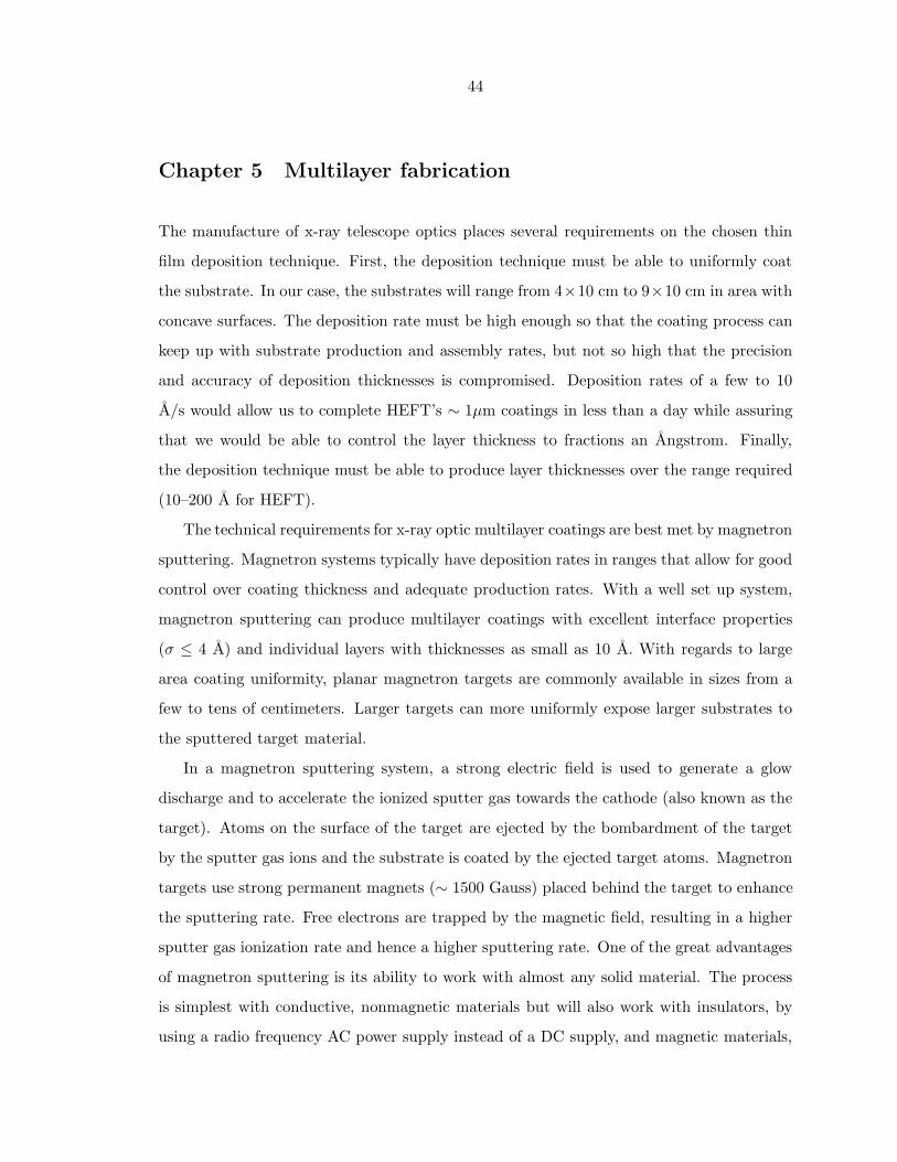
44

Chapter 5 Multilayer fabrication

The manufacture of x-ray telescope optics places several requirements on the chosen thin

film deposition technique. First, the deposition technique must be able to uniformly coat

the substrate. In our case, the substrates will range from 4×10 cm to 9×10 cm in area with

concave surfaces. The deposition rate must be high enough so that the coating process can

keep up with substrate production and assembly rates, but not so high that the precision

and accuracy of deposition thicknesses is compromised. Deposition rates of a few to 10

A/s would allow us to complete HEFT’s ∼ 1µm coatings in less than a day while assuring

that we would be able to control the layer thickness to fractions an Angstrom. Finally,

the deposition technique must be able to produce layer thicknesses over the range required

(10–200 A for HEFT).

The technical requirements for x-ray optic multilayer coatings are best met by magnetron

sputtering. Magnetron systems typically have deposition rates in ranges that allow for good

control over coating thickness and adequate production rates. With a well set up system,

magnetron sputtering can produce multilayer coatings with excellent interface properties

(σ ≤ 4 A) and individual layers with thicknesses as small as 10 A. With regards to large

area coating uniformity, planar magnetron targets are commonly available in sizes from a

few to tens of centimeters. Larger targets can more uniformly expose larger substrates to

the sputtered target material.

In a magnetron sputtering system, a strong electric field is used to generate a glow

discharge and to accelerate the ionized sputter gas towards the cathode (also known as the

target). Atoms on the surface of the target are ejected by the bombardment of the target

by the sputter gas ions and the substrate is coated by the ejected target atoms. Magnetron

targets use strong permanent magnets (∼ 1500 Gauss) placed behind the target to enhance

the sputtering rate. Free electrons are trapped by the magnetic field, resulting in a higher

sputter gas ionization rate and hence a higher sputtering rate. One of the great advantages

of magnetron sputtering is its ability to work with almost any solid material. The process

is simplest with conductive, nonmagnetic materials but will also work with insulators, by

using a radio frequency AC power supply instead of a DC supply, and magnetic materials,

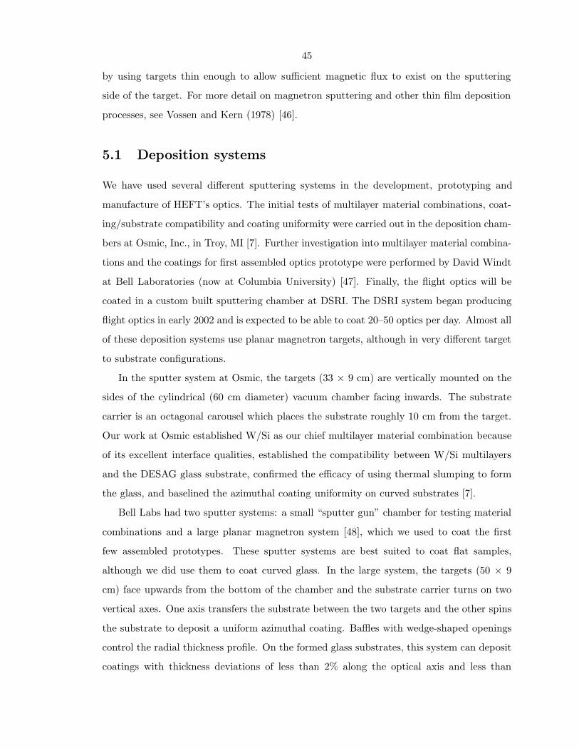
45

by using targets thin enough to allow sufficient magnetic flux to exist on the sputtering

side of the target. For more detail on magnetron sputtering and other thin film deposition

processes, see Vossen and Kern (1978) [46].

5.1 Deposition systems

We have used several different sputtering systems in the development, prototyping and

manufacture of HEFT’s optics. The initial tests of multilayer material combinations, coat-

ing/substrate compatibility and coating uniformity were carried out in the deposition cham-

bers at Osmic, Inc., in Troy, MI [7]. Further investigation into multilayer material combina-

tions and the coatings for first assembled optics prototype were performed by David Windt

at Bell Laboratories (now at Columbia University) [47]. Finally, the flight optics will be

coated in a custom built sputtering chamber at DSRI. The DSRI system began producing

flight optics in early 2002 and is expected to be able to coat 20–50 optics per day. Almost all

of these deposition systems use planar magnetron targets, although in very different target

to substrate configurations.

In the sputter system at Osmic, the targets (33 × 9 cm) are vertically mounted on the

sides of the cylindrical (60 cm diameter) vacuum chamber facing inwards. The substrate

carrier is an octagonal carousel which places the substrate roughly 10 cm from the target.

Our work at Osmic established W/Si as our chief multilayer material combination because

of its excellent interface qualities, established the compatibility between W/Si multilayers

and the DESAG glass substrate, confirmed the efficacy of using thermal slumping to form

the glass, and baselined the azimuthal coating uniformity on curved substrates [7].

Bell Labs had two sputter systems: a small “sputter gun” chamber for testing material

combinations and a large planar magnetron system [48], which we used to coat the first

few assembled prototypes. These sputter systems are best suited to coat flat samples,

although we did use them to coat curved glass. In the large system, the targets (50 × 9

cm) face upwards from the bottom of the chamber and the substrate carrier turns on two

vertical axes. One axis transfers the substrate between the two targets and the other spins

the substrate to deposit a uniform azimuthal coating. Baffles with wedge-shaped openings

control the radial thickness profile. On the formed glass substrates, this system can deposit

coatings with thickness deviations of less than 2% along the optical axis and less than

46

5% in the substrate’s azimuthal direction. We used these optics on the first HEFT optic

prototype to test the accuracy of the mounting technique and for high-energy reflectance

measurements of the multilayer designs. Although we measured the azimuthal uniformity,

these results do not reflect flight optic uniformity because the substrate to target geometry

is so different from the DSRI system.

The DSRI sputtering chamber is similar to the Osmic system in that the substrates are

mounted on a carousel and the targets are positioned vertically. Unlike the Osmic system,

however, the DSRI system has the targets (50 × 3.8 cm) positioned inside the vacuum

chamber facing radially outward and the substrates are mounted on the 1 m diameter

carousel facing inward. The substrate to target distance can be adjusted by moving the

targets along a radial track; presently, the distance is set at 10.8 cm. The optics are

mounted with their optical axes perpendicular to the length of the targets. With the

perpendicular arrangement, changes in substrate to target distance and angle along the

optical axis adversely affect the coating uniformity in that direction, but with the large

carousel diameter in the DSRI system, these effects are negligible. Along the optical axis,

the perpendicular mounting results in a 2% variation in substrate to target distance and a

6variation in deposition angle. We can control the uniformity along the azimuthal direction

of the optic by masking the sputter target to alter its lengthwise emission profile. The

coating uniformity characteristics of this configuration have been measured with 8.048 keV

R vs. θ scans and the results are displayed in Figure 5.1.

5.2 High-energy measurements of graded multilayer designs

At all of the coating facilities, we had access to 8.048 keV (Cu anode) x-ray systems for

measuring reflectance vs. incidence angle. We use R vs. θ measurements to find the layer

thicknesses and average interface width of our coatings. Theoretically, 8 keV measurements

are adequate to fully characterize the coatings for use at higher energies because the x-rays

fully penetrate the coating and they probe surface irregularities over the full range of length

scales, from the beam footprint to the sub-Angstrom scale. Nevertheless, in order to excise

any doubt that the mirrors would work as designed over the operating energy band (20–70

keV), we tested the optics at energies up to 170 keV.

We built a nested mirror prototype section and brought it to the European Synchrotron

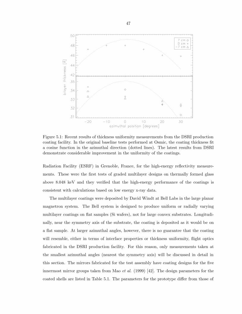
47

Figure 5.1: Recent results of thickness uniformity measurements from the DSRI productioncoating facility. In the original baseline tests performed at Osmic, the coating thickness fita cosine function in the azimuthal direction (dotted lines). The latest results from DSRIdemonstrate considerable improvement in the uniformity of the coatings.

Radiation Facility (ESRF) in Grenoble, France, for the high-energy reflectivity measure-

ments. These were the first tests of graded multilayer designs on thermally formed glass

above 8.048 keV and they verified that the high-energy performance of the coatings is

consistent with calculations based on low energy x-ray data.

The multilayer coatings were deposited by David Windt at Bell Labs in the large planar

magnetron system. The Bell system is designed to produce uniform or radially varying

multilayer coatings on flat samples (Si wafers), not for large convex substrates. Longitudi-

nally, near the symmetry axis of the substrate, the coating is deposited as it would be on

a flat sample. At larger azimuthal angles, however, there is no guarantee that the coating

will resemble, either in terms of interface properties or thickness uniformity, flight optics

fabricated in the DSRI production facility. For this reason, only measurements taken at

the smallest azimuthal angles (nearest the symmetry axis) will be discussed in detail in

this section. The mirrors fabricated for the test assembly have coating designs for the five

innermost mirror groups taken from Mao et al. (1999) [42]. The design parameters for the

coated shells are listed in Table 5.1. The parameters for the prototype differ from those of

48

the final design, listed in Table 4.3, because at the time, the optimization was calculated

by a grid search, as described in Mao et al. (1999), rather than the iterative search that is

currently implemented.

Table 5.1: HEFT prototype design parameter.group N c Γ t [µm] FOM [cm2]

1 150 0.225 0.40 0.664 0.4802 200 0.230 0.40 0.793 0.5523 250 0.220 0.40 0.934 0.7294 250 0.225 0.40 0.896 0.7925 300 0.220 0.40 1.014 0.832

The coated samples were assembled into a single-reflection cylindrical prototype at Col-

orado Precision Products, Inc. (CPPI). The quadrant-section shells are each separated by

five graphite rods positioned at 0, ±22, and ±44. The shells are 20 cm in length and were

formed to 8.3, 8.4, 8.5, 8.6 and 8.7 cm radii of curvature. Specular reflectivity measurements

were taken at azimuthal angles out to ±40to determine both the coating uniformity and

the imaging performance, or figure, of the assembled optics. The uniformity was found to

be better than cosine distributed, with the bilayer thickness falling off by less than 10% at

±40[49]; however, these results will not necessarily carry over to the production mirrors be-

cause of the differences in deposition chamber geometry. The imaging performance was very

promising, with a calculated half power diameter (HPD) of 35.1′′ for the single-reflection

prototype [50]. This would translate to an HPD of 49.6′′ for the 2-reflection telescope.

The measurements closest to the symmetry axis, at φ = +5and φ = −8, verified the

performance of the coating designs with measurements from 34 to 170 keV. Determining

the bilayer distribution of a graded multilayer coating from a reflectivity scan is much more

difficult than determining the layer thicknesses of a non-depth graded coating. In modeling

the reflectivity measurements, we assume that the bilayer thickness distribution only differs

from point to point on the coating by a multiplicative parameter. The observed minimum

bilayer thickness can be deduced by a sharp drop in reflectivity just above the incidence angle

corresponding to first order Bragg reflection off the bottom-most layer of the coating. The

reflectivity is then calculated by using the design-specified values of b and c (from Equation

3.20) and adjusting a so that the minimum bilayer thickness matches the thickness deduced

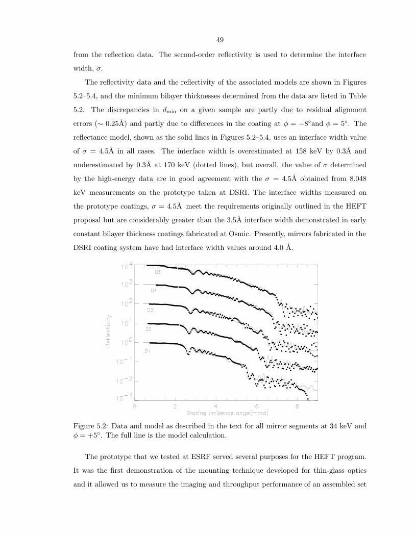
49

from the reflection data. The second-order reflectivity is used to determine the interface

width, σ.

The reflectivity data and the reflectivity of the associated models are shown in Figures

5.2–5.4, and the minimum bilayer thicknesses determined from the data are listed in Table

5.2. The discrepancies in dmin on a given sample are partly due to residual alignment

errors (∼ 0.25A) and partly due to differences in the coating at φ = −8and φ = 5. The

reflectance model, shown as the solid lines in Figures 5.2–5.4, uses an interface width value

of σ = 4.5A in all cases. The interface width is overestimated at 158 keV by 0.3A and

underestimated by 0.3A at 170 keV (dotted lines), but overall, the value of σ determined

by the high-energy data are in good agreement with the σ = 4.5A obtained from 8.048

keV measurements on the prototype taken at DSRI. The interface widths measured on

the prototype coatings, σ = 4.5A meet the requirements originally outlined in the HEFT

proposal but are considerably greater than the 3.5A interface width demonstrated in early

constant bilayer thickness coatings fabricated at Osmic. Presently, mirrors fabricated in the

DSRI coating system have had interface width values around 4.0 A.

Figure 5.2: Data and model as described in the text for all mirror segments at 34 keV andφ = +5. The full line is the model calculation.

The prototype that we tested at ESRF served several purposes for the HEFT program.

It was the first demonstration of the mounting technique developed for thin-glass optics

and it allowed us to measure the imaging and throughput performance of an assembled set

50

Figure 5.3: Data and model as described in the text for all mirror segments at 65 keV andφ = −8. The full line is the model calculation.

of optics. The consistent agreement between calculated and measured reflectance with a

single value for of σ over the HEFT bandpass experimentally validate the relevance of 8

keV measurements to performance at those energies.

Table 5.2: Minimum bilayer thickness [A] determined by hard x-ray measurements con-ducted at ESRF.

Mirror 34 keV 65 keV 158 keV 170 keVSegment φ = 5 -8 -8 -8

D1 34.6 34.3D2 30.8 30.2D3 29.4 29.6 29.6D4 27.6 27.5 28.8D5 26.4

51

Figure 5.4: Data and model as described in the text for mirror segment D3 at 170 keVand D4 at 158 keV. In both cases, the azimuthal position is φ = −8. The solid lines showthe calculated reflectivity vs. incidence angle assuming σ = 4.5A. The dotted lines arecalculated reflectivities for σ = 4.2A (D4, 158 keV) and σ = 4.8A (D3, 170 keV).

52

Chapter 6 The Serendipitous Extragalactic X-ray Source

Identification survey

The 1999 launch of the Chandra X-ray Observatory, with subarcsecond angular resolution

in the 0.5–10 keV band, reinvigorated research on the extragalactic x-ray background. Long

exposures, 105–106 s, have resolved 70–80% of this energy band’s extragalactic x-ray emis-

sion into discrete sources [19, 20, 51]. Apart from verifying the existence of these faint x-ray

sources and perhaps determining the spectral indices of their continuum emission, little

else on the individual sources can be gleaned from the x-ray images. In order to study the

nature of extragalactic x-ray sources, we must use other wavelength bands. Chandra’s sub-

arcsecond angular resolution allows for reliable optical identification of the x-ray sources,

making it possible for us to study the optical spectra of the newly located extragalactic

x-ray sources.

One of the shortcomings of the deep observations is their limited sky coverage. With a

field of view roughly 0.07 square degrees, the Chandra deep-field (CDF) surveys find several

hundred sources to a limiting flux of around 10−16 erg cm−2 s−1 in the Chandra soft (0.5–2

keV) and hard (2–10 keV) bands. At the bright end (∼ 10−14 erg cm−2 s−1) of the deep

field survey population, however, the statistics are poor. In the soft band, CDF surveys find

fewer than five bright sources per field, and in the 2–10 keV band they only find around 20

bright sources per field [52, 20]. The bright end of the CDF survey population is of interest

because sources with observed fluxes around 10−14 erg cm−2 s−1 in the Chandra soft and

hard bands contribute to a large fraction of the extragalactic x-ray emission [19, 51]. The

Serendipitous EXtragalactic Source Identification (SEXSI) survey complements the deep

Chandra observations by using a large number of medium depth (20 – 200 ks) exposures.

Presently, the SEXSI survey covers an area of roughly 2 square degrees to a maximum depth

of 10−15 erg cm−2 s−1 in the 2–10 keV band. The wide area covered by the SEXSI survey

has yielded more than 1200 sources covering the bright end of the CDF survey populations.

The SEXSI survey uses Chandra’s public archived data: performance verification data,

in-flight calibration data, and data from other observing programs. We select imaging

observations of high galactic latitude fields (|b| > 20) using the ACIS detectors. The

53

distribution of the selected fields’ exposure times are plotted in Figure 6.1. More detailed

information on the individual fields are listed in Table 6.1.

Figure 6.1: Exposure time distribution of the SEXSI survey. The heavy line shows theexposure times of the 10 fields for which we have optical spectroscopic data.

As of the present date, optical imaging of the SEXSI fields is 65% complete by source

count in the R (or r′) band and spectrocopic follow-up covers 16% of sources in the survey

over the 400–1000 nm band. The pace of optical imaging in other filter bands will increase

due to the availability of large area (24′× 24′ FOV) optical cameras such as the Large Format

Camera (LFC) at Palomar and the 8k Camera at the MDM 2.4 m telescope. Previous optical

cameras have had fields of view on the order of 10′, so the large area cameras increase our

observing efficiency by more than a factor of 4. Optical spectroscopic coverage proceeds

at a much slower pace than imaging but it also yields much more information about the

sources: redshift, luminosity, and spectral classification. The following discussion on the

SEXSI survey will concentrate on the ten fields (designated with bold type in Table 6.1

and with the heavy line in Figure 6.1) for which we have substantial optical spectroscopic

coverage.

54

Table 6.1: Status of optical spectroscopy follow-up observations.Target ra/dec exp ACIS # x-ray R-band spectr.

[ks] center:chips srcs. done doneNGC 891 02:22:33 +42:20:57 51 S:235-8 54 41 0AWM 7 02:54:28 +41:34:47 48 I:0-367 34 28 0XRF 011130 03:05:28 +03:49:59 30 I:0-3 38 27 0NGC 1569 04:30:49 +64:50:54 97 S:0-357 47 44 153C 123 04:37:55 +29:40:14 47 S:235-8 29 14 0CL 0848 08:48:32 +44:53:56 186 I:0-367 85 74 55RXJ 0910 09:10:39 +54:19:57 171 I:0-36 104 64 01156+295 11:59:32 +29:14:44 49 I:0-367 54 52 1NGC 4244 12:17:30 +37:48:32 49 S:235-8 36 28 7NGC 4631 12:42:07 +32:32:30 59 S:235-8 43 32 2HCG 62 12:53:08 –09:13:27 49 S:35-8 43 35 19RXJ 1317 13:17:12 +29:10:18 111 I:0-36 71 0 0BD 1338 13:38:25 +29:31:05 38 I:0-367 51 36 30RXJ 1350 13:50:55 +60:05:09 58 I:0-36 38 383C 295 14:11:20 +52:12:21 23 S:235-8 11 5 5GRB 010222 14:52:12 +43:01:44 18 S:235-8 26 23 13NGC 5846 15:06:27 +01:36:12 30 S:235-8 27 0QSO 1508 15:09:58 +57:02:32 89 S:0-367 52 44 0MKW 3S 15:21:52 +07:42:32 57 I:0-368 38 27 0ABELL 2104 15:40:04 –03:17:30 49 S:235-8 36 0ABELL 2142 15:58:20 +27:13:45 30 S:235-8 7 6 5MS 1621 16:23:36 +26:33:50 30 I:0-36 31 28 0NGC 6251 16:32:32 +82:32:28 40 I:0-367GRB 000926 17:04:11 +52:46:34 32 S:235-8 32 26 22RXJ 1716 17:16:52 +67:08:31 52 I:0-36 48 43 30NGC 6543 17:58:29 +66:38:29 46 S:4-9 25 7 0XRF 011030 20:43:32 +77:16:43 67 S:23678MS 2053 20:56:22 –04:37:44 44 I:0-36 51 40 16RXJ 2247 22:47:29 +03:37:13 49 I:0-36 56Q2345+007 23:48:20 +00:57:21 74 S:123678 43 22 0totals 1210 784 220

55

Chapter 7 Data reduction

7.1 X-ray reduction

SEXSI uses high galactic latitude (|b| > 20) imaging observations using the ACIS camera

on board the Chandra X-ray Observatory (CXO). The ACIS camera consists of ten 1024 ×

1024 CCD detectors, each with a 8.4′× 8.4′ field of view. Four chips constitute the ACIS-I

(imaging) array, arranged in a square and tilted so that they are tangent to the focal plane

of the mirror array. The remaining six which make up the ACIS-S (spectroscopy) array are

arranged linearly on the Rowland circle of the gratings. In the CXO documentation, ACIS

chips are sometimes referred to as ACIS-I 0–3 and ACIS-S 0–5, and sometimes referred to

as ACIS 0–9, with 0–3 corresponding to the ACIS-I array, and 5–9 corresponding to the

ACIS-S array (see Figure 7.1). In all of the processing software that I have written for data

reduction, I use the second convention, and I will use it for all references to the ACIS arrays

in this thesis.

When using the ACIS camera for imaging observations, users can specify the location

of the optical axis either on the ACIS-I array or on the ACIS-S array. With ACIS-I obser-

vations, the optical axis is located off-center on chip 3, and with ACIS-S observations, the

optical axis is located on chip 7. Some observers choose the ACIS-S array for imaging be-

cause chips 5 and 7 are back-side illuminated, giving these chips better low energy quantum

efficiency but also, initially, poorer energy resolution. During Chandra’s calibration phase,

radiation damage from protons degraded the energy resolution of the front-side illuminated

chips, making their resolution comparable to that of the back-side illuminated chips. For

detecting serendipitous sources, ACIS-I observations are ideal. The point spread function

(PSF) of the mirrors remains at the arcsecond level on all of the I chips, and brighter sources

can be detected on chips 6 and 7 on the S array, although with much poorer angular res-

olution. With ACIS-S centered observations, the chips from which we can extract sources

are 6,7, and 8 on the S array and 2 and 3 on the I array. The PSF and effective area on the

remaining chips are generally too poor to use.

X-ray raw data from CCDs differs from optical and other long wavelength raw data

56

S0 S1 S2 S3 S4 S5

w168c4r w140c4r w182c4r w134c4r w457c4 w201c3r

I0 I1

I2 I3

ACIS-S

x

18 pixels = 8".8

22 pixels = 11"

~22 pixels ~11" not

0 1

2 3

4 5 6 7 8 9

constant with Z

Top

Bottom

330 pixels = 163"

w203c4r w193c2

w215c2rw158c4r

colu

mn

CCD Key NodeDefinitions

Row/ColumnDefinition

CoordinateOrientations

one

two

thre

e

(aimpoint on S3 = (252, 510))

node

zer

o

row. .

+

(aimpoint on I3 = (962, 964))

ACIS-I

Frame Store

Pixel (0,0)

Image Region

BI chip indicator

+Z

Pointing

Coordinates

+Y

Offset

TargetY∆+

Z∆+

Coordinates+Z

-Z

Sim Motion

Figure 7.1: ACIS flight focal plane layout. Courtesy of Chandra Science Center [1].

because the detector is operated as photon counter with energy discrimination rather than

as a flux integrator. For each photon detected, the location of the triggering pixel and

the energy deposited in that pixel and its 8 nearest neighbors are recorded. To distinguish

between photon and cosmic-ray events, event grades are defined, based on which of the

neighboring pixels exceed a “split” threshold. The event grades defined for the ASCA

mission are often used for data from other missions. The definition of the ASCA event

grades can be found in The ASCA Data Reduction Guide [53].

We use the wavelet detection program, wavdetect, in the CIAO software package for

source detection. wavdetect operates on images, not event lists, so we create images of

each chip from the event list, using ASCA event grades 0, 2, 3, 4, and 6. On-axis chips (0–3

for ACIS-I pointings and 7 for ACIS-S pointings) are not rebinned, while the remaining

off-axis chips are 2×2 rebinned. Most of our sources are not detected with enough photons

to construct an energy spectrum of the source, we use count ratios between bands to get a

crude idea of the source spectrum. For each chip, we create a soft-band image (0.3–2.1 keV)

57

and a hard-band image (2.1–7 keV). The hard and soft energy bands are chosen to cover

the range of energies for which Chandra has substantial effective area (see Figure 7.2). We

separate the bands at 2.1 keV to coincide with the large change in the Chandra mirrors’

reflectance due to the Ir-M photoelectric edge.

Figure 7.2: Chandra effective area for front- and back-side chips. Courtesy of ChandraScience Center [1].

Under certain conditions, usually at far off-axis positions, the wavdetect derived posi-

tions appear to be offset in random directions from the centroid position of the source by

several arcseconds, in one case (NGC 1569, d2001) being 8′′ off the centroid of the source

(see Figures 7.3 and 7.4). Similar problems with wavdetect derived positions have been

reported by Brandt et al. (2001) [54]. Most investigators have been using wavdetect de-

rived positions for x-ray sources detected by CXO, and we also use those positions, except

in those cases where the position is obviously far from the centroid. We find the object’s

58

centroid position by iteratively calculating the centroid with the PSF radius, as defined by

the off-axis angle of the source. The routine converges when the shift in position is less than

5% of the PSF. The position problem with wavdetect tends to occur with sources at large

off-axis angles (large PSF’s), so in order to quantitatively differentiate between good and

bad wavdetect positions, we calculate the product of the absolute and PSF normalized ra-

dial shifts, ∆r2/PSF. Empirically, we find that using a cutoff of ∆r2/PSF = 0.8 agrees with

what we would conclude from visual inspection. For those sources where ∆r2/PSF > 0.8,

we use the centroid position, otherwise, we stay with the wavdetect position. A scatter

plot of ∆r2/PSF vs. wavdetect derived SNR is shown in Figure 7.5.

d2011

d2010

d2009

d2008

d2007

d2005

d2004d2003

d2002

d2001

d2011

d2010

d2009

d2008

d2007

d2005

d2004d2003

d2002

d2001

NGC 1569

Figure 7.3: A pathological case demonstrating problems with wavdetect’s determination ofsource positions. Left: NGC 1569, chip 2, hard-band CXO image. Data courtesy of CrystalMartin. Right: P60, CCD-13 R band image of the same field. The green circles mark thewavdetect positions. The blue markers indicate centroid positions that do not meet thecriteria to supersede the wavdetect positions and red markers indicate positions where thecentroid position supersedes the wavdetect position. The radii of the markers correspondto the PSF of the mirror array at that location. The north arm of the compass rose is 60′′

and the east arm is 30′′.

After the source positions are checked and adjusted as prescribed, we calculate the

source flux and detection probability. Because of the CXO’s fine angular resolution and low

background, we are often able to detect sources with as few as 5 or 10 photons. Based on

an estimate of the local background rate, we calculate a detection probability and reject

59

c6014

c6012

c6011c6010

c6009

c6008

c6007

c6006

c6005

c6004

c6003

c6002

c6001

c6014

c6012

c6011c6010

c6009

c6008

c6007

c6006

c6005

c6004

c6003

c6002

c6001

HCG 62

Figure 7.4: More typical source position results from wavdetect. Here, source c6007 hasthe largest ∆r2/PSF offset, at 0.21, followed by c6005 with a 0.20 offset. Both are wellbelow our criteria for using centroid-derived positions. Left: HCG 62, chip 6, hard-bandCXO image. Data courtesy of Jan Vrtilek. Right: MDM 2.4 m, Eschelle camera R bandimage of the same field. The green circles mark the wavdetect positions. The blue markersindicate centroid positions. The radii of the markers correspond to the PSF of the mirrorarray at that location. The north arm of the compass rose is 60′′ and the east arm is 30′′.

sources for which the detection probability is less then 10−6. In order to estimate the

flux from these sources, we fit the number of detected photons to a power law spectrum

F = kE−Γ erg/(cm2 s keV) with the index, Γ = 1.5. At this point, we have completed the

main part of the x-ray data processing. We have the position, PSF, hard and soft fluxes,

and a measure of the detection confidence of each source.

7.2 Optical reduction

For optical imaging of the Chandra fields, we use the 60 and 200 inch telescopes at Palomar

and the MDM 2.4 meter telescope. Until the large field of view detectors (LFC on the P200

and the 8k camera on the MDM 2.4 m) became reliable for general use in the past year,

multiband optical imaging was very difficult. Both LFC and the 8k camera have 24′×24′

fields of view, allowing them usually to cover an entire Chandra field with a single pointing.

For comparison, CCD-13, used on the P60, only has a 12.5′×12.5′ field of view and the

60

Figure 7.5: ∆r2/PSF vs. wavdetect derived SNR for hard-band detections from NGC1569, chip 2 and HCG 62, chip 6. The dotted line indicates the cut, above which we adoptthe centroid derived position

previous cameras on the P200 (Cosmic) and MDM 2.4 m (Eschelle) had even smaller fields

of view. The availability of large detectors in optical astronomy is important for the SEXSI

project because it allows us to efficiently take multiband optical images of the Chandra

fields. Most of SEXSI’s optical data were taken with a Johnson-Cousins R band filter

because the large cameras were not available early on and we rarely had enough observing

time to use other filters. With LFC, we use Sloan filters, g′, r′, i′, and z′, and with the 8k,

we use Johnson-Cousins filters, B, V , R, and I. In each filter band, our goal has been to

obtain images with a limiting magnitude of 24–25.

For optical spectroscopy of the counterparts, we use the Low Resolution Imaging Spec-

trometer (LRIS) on Keck [55] and Doublespec on the P200. LRIS has a 7.5′× 6′ field of

view and supports slit masks. Typically, given the source density of our fields, we fit 5–20

mR < 23 sources on a mask. The spectra of sources fainter than mR = 23 generally require

exposure times greater than the two hours we allot to each mask. Slit masks are fabricated

well before the observing run and cannot be changed during the night, so we specify 1.4′′

wide slits on our masks even though the PSF due to atmospheric turbulence (“seeing”) at

Keck is usually subarcsecond. We use Doublespec mainly for brighter sources that do not

61

fit well onto LRIS slit masks because it is impractical to use the P200 on sources fainter

than mR = 21. Doublespec is a single-slit instrument and the different sized slits can be

interchanged during the night. We use the 1.0′′, 1.5′′, or 2.0′′ slits depending on the seeing.

Typical seeing at the P200 is 1.0–1.5′′. Table 7.1 details the setup of the spectrometers.

Table 7.1: Spectrometer setup parameters.Doublespec LRIS

blue red blue redgrating pitch [lines/mm] 600 158 300 150λblaze [A] 3780 7560 5000 7500λcenter [A] 4500 7500 N.A. 7000–8500dichroic D52 (5200 A) D560 (5600 A)slit width [arcsec] 1.0, 1.5, or 2.0 1.4

7.2.1 Imaging

The details of the optical image reduction described in this section apply to the small format

cameras. With the large format cameras, astrometry is more difficult to solve because of

the substantial spatial distortions at large off-axis angles (5′– 10′). The basic outline of

data reduction is the same for small and large format cameras; however, I have not been

directly involved in the more complex processing of the large format cameras.

We subtract the bias level from the raw images and flatten their exposures according to

the standard methods provided by the IRAF software package [56]. Except in rare cases,

we use bias frames taken from the same night that the images are taken. For the flat field

images, we either use dome flats or we make a sky flat by combining all the images from

the night, including the twilight flats, and using min/max rejection to remove the stars.

The next step in optical data reduction involves stacking the images and solving for

the astrometry. Both of these tasks require knowledge of the (x, y) positions of the objects

in the fields. We use the DOPHOT software package to locate all of the nonsaturated,

point-like objects in the images. We use starmatch, an object matching program written

by Doug Reynolds (University of Washington), both to align the images before stacking

and to solve the astrometry of the final, combined image. Cosmic ray traces are cleaned

from the final image with the crreject rejection subroutine within IRAF, which uses a

one-sided sigma clipping algorithm. The astrometry is determined via comparison with the

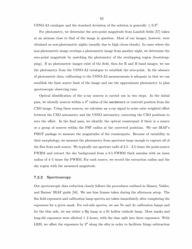
62

USNO-A2 catalogue and the standard deviation of the solution is generally ≤ 0.3′′.

For photometry, we determine the zero-point magnitude from Landolt fields [57] taken

at an airmass close to that of the image in question. Most of our images, however, were

obtained on non-photometric nights (usually due to high cirrus clouds). In cases where the

non-photometric image overlaps a photometric image from another night, we determine the

zero-point magnitude by matching the photometry of the overlapping region (bootstrap-

ping). If no photometric images exist of the field, then for R and B band images, we use

the photometry from the USNO-A2 catalogue to establish the zero-point. In the absence

of photometric data, calibrating to the USNO-A2 measurements is adequate in that we can

establish the faint source limit of the image and use the approximate photometry to plan

spectroscopic observing runs.

Optical identification of the x-ray sources is carried out in two steps. In the initial

pass, we identify sources within a 5′′ radius of the wavdetect or centroid position from the

CXO image. Using these sources, we calculate an x-ray signal to noise ratio weighted offset

between the CXO astrometry and the USNO astrometry, correcting the CXO positions to

zero the offset. In the final pass, we identify the optical counterpart if there is a source

or a group of sources within the PSF radius at the corrected positions. We use IRAF’s

PHOT package to measure the magnitudes of the counterparts. Because of variability in

their morphology, we measure the photometry from apertures large enough to capture all of

the flux from each source. We typically use aperture radii of 2.5 – 3.5 times the point-source

FWHM and extract the sky background from a 0.5 FWHM thick annulus with an inner

radius of 4–5 times the FWHM. For each source, we record the extraction radius and the

sky region with the measured magnitude.

7.2.2 Spectroscopy

Our spectroscopic data reduction closely follows the procedures outlined in Massey, Valdes,

and Barnes’ IRAF guide [58]. We use bias frames taken during the afternoon setup. The

flat field exposures and calibration lamp spectra are taken immediately after completing the

exposures for a given mask. For red-side spectra, we use Ne and Ar calibration lamps and

for the blue side, we use either a Hg lamp or a Fe hollow cathode lamp. Most masks and

long-slit exposures were allotted 1–2 hours, with the time split into three exposures. With

LRIS, we offset the exposures by 3′′ along the slits in order to facilitate fringe subtraction

63

at long wavelengths (∼> 7200A). The offsets were not performed with Doublespec because

the controls are not in place at the P200 to track the telescope along the slit.

Daniel Stern’s bogus script was crucial for the timely reduction of the slit mask data.

The script takes as input the debiased slit mask images and outputs the images (2-D spectra)

from the individual slits as separate files. The output images from a given mask are aligned

on their dispersion axes in order to facilitate batch processing of the wavelength calibration.

The script also performs cosmic-ray rejection, flat fielding, sky subtraction, and fringe

subtraction on the images and aligns and stacks the individual exposures. The cosmic-

ray rejection routine within bogus, xzap, can be overzealous and will occasionally remove

or severely alter some narrow spectral features. Consequently, we always compare xzap-ed

and non-xzap-ed images to safeguard against the removal of spectral lines by the cosmic-ray

rejection routine. Although bogus is primarily a script for slit mask data, I also used it to

process Doublespec long-slit spectra in order to maintain consistency in the data processing.

For extraction of the spectra from the images, wavelength calibration, and flux cali-

bration, I used the doslit script in the noao/kpnoslit IRAF package. The extraction

aperture width was set to where the spatial profile of the object fell to 5% of its peak value.

We fit the extraction trace with a Legendre polynomial, typically fifth order, and use the

same set of parameters to extract the lamp spectrum. The wavelength calibrations, mea-

sured from the extracted lamp spectrum required a separate third to fifth order Legendre

polynomial fit. For flux calibration standards, we used the sources investigated by Oke and

Gunn (1983) [59] and Massey and Gronwall (1990) [60].

64

Chapter 8 Results from the SEXSI survey

The SEXSI survey presently consists of over 1200 CXO hard band (2.1–7.0 keV) selected

sources from 31 fields. Roughly half of the sources (582) have been optically identified and

a quarter (202) of them have no optical counterpart down to mR = 24. For the remaining

sources, an eighth are undetected in the optical at mR = 23 and the final eighth have yet

to be imaged in the optical. In this chapter, I discuss our classification scheme for objects

with optical spectroscopic data and present preliminary results of the survey. The results

come from the ten fields, noted in boldface type in Table 6.1, for which we have optical

spectroscopic data on a significant number of the counterparts.

8.1 Spectroscopic classification

Based on the optical spectroscopic data, we classify the sources as active galaxies, normal

galaxies or stars. The active galaxies are further subdivided into broad and narrow line

QSOs and Seyfert galaxies. The nonactive galaxies are subdivided into emission line and

absorption line (early-type) galaxies. The stars we detect are typically M stars. There are

a few cases where the optical image suggests that the source may be a cluster of galaxies,

but we have not yet spectroscopically followed up any of these sources.

Our classification of active galaxies follows the criteria outlined by Schmidt et al. (1998)

[12]. We identify as AGN sources with broad emission lines or lines from highly ionized

species. For low redshift objects, we look for broad Hα or Hβ emission (see Figure 8.1). For

higher redshift objects, we look for Mgiiλ2799A and Ciii]λ1909A lines and, if accessible,

Civλ1549A and Lyα emission. Within the AGN category, we differentiate between the

narrow and broad line varieties with a cut at line widths of the permitted lines (Civ, Ciii],

Mgii) at 2000 km/s. Examples of broad and narrow line AGN optical spectra are shown

in Figures 8.2 and 8.3. Schmidt uses the [Nev]λ3426A line to identify soft x-ray emitting

galaxies and classifies them as AGN when their luminosity exceeds 1043 erg cm−2 s−1. We

find many galaxies without any obvious AGN characteristics in the 1042–1044 erg cm−2 s−1

luminosity range.

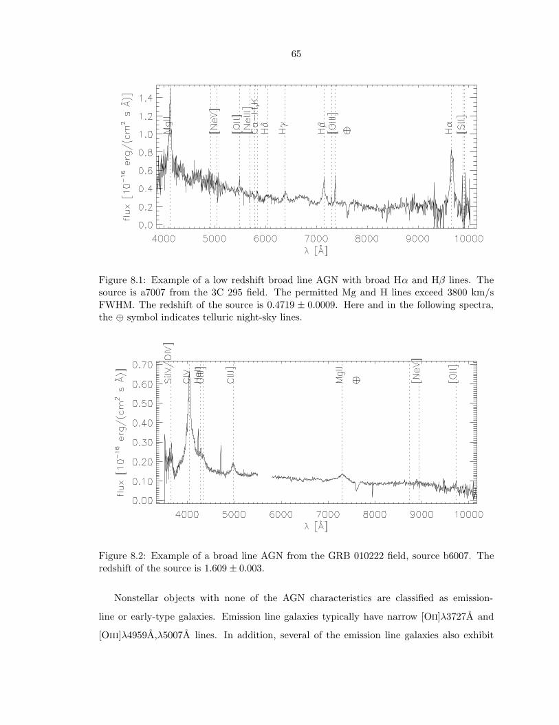
65

Figure 8.1: Example of a low redshift broad line AGN with broad Hα and Hβ lines. Thesource is a7007 from the 3C 295 field. The permitted Mg and H lines exceed 3800 km/sFWHM. The redshift of the source is 0.4719 ± 0.0009. Here and in the following spectra,the ⊕ symbol indicates telluric night-sky lines.

Figure 8.2: Example of a broad line AGN from the GRB 010222 field, source b6007. Theredshift of the source is 1.609 ± 0.003.

Nonstellar objects with none of the AGN characteristics are classified as emission-

line or early-type galaxies. Emission line galaxies typically have narrow [Oii]λ3727A and

[Oiii]λ4959A,λ5007A lines. In addition, several of the emission line galaxies also exhibit

66

Figure 8.3: Example of a narrow line AGN from the HCG 62 field, source c7022. The widthsof the permitted emission lines are at resolution limit of the spectrograph. The redshift ofthe source is 1.154 ± 0.002.

Figure 8.4: Example of an emission line galaxy from the GRB 000926 field, source b3004.The red-side flux has been multiplied by 1.4 to compensate for a discepancy in the fluxcalibration between the red and blue cameras. The redshift of the source is 0.2587±0.0006.

the Ca-K (λ3933A) and Ca-H (λ3967A) absorption lines. Absorption line galaxies constitute

our smallest and most restricted class. The spectra of these sources are only identifiable by

the Ca-K and Ca-H absorption lines or in some cases, the D4000 spectral break. Examples

of emission line and absorption line galaxies are shown in Figures 8.4 and 8.5.

67

Figure 8.5: Example of an absorption line galaxy from the NGC 1569 field, source d3008.The redshift of the source is 0.753 ± 0.001.

There is little doubt that the sources we classify as AGN do, in fact, contain active

nuclei, but the classification of the nonactive galaxies is less clear. Several of the AGN

identified on the basis of broad Mgii emission also have the emission and absorption lines

characteristic of normal galaxies. At lower redshifts, due to incomplete spectral coverage,

we cannot be certain that the sources we classify as normal galaxies do not also have shorter

wavelength lines associated with AGN. Similarly, we classify absorption line galaxies on the

basis of incomplete information. With broader spectral coverage or longer exposures, these

sources may be reclassified as emission-line galaxies or even AGN.

8.2 Preliminary results from SEXSI

The 10 fields from which we draw our preliminary results contain roughly 398 hard band

(2.1–7 keV) selected sources. We have categorized 211 of these objects using optical spec-

troscopic data and there are another 75 counterparts that await spectroscopic observation.

Of the remaining sources, 5 have had no optical follow up, 33 are optically faint (mR > 24),

and 74 require deeper optical observations to determine if the optical emission from the

source is bright enough for spectroscopy.

68

8.2.1 Comparisons with deep-field surveys

From the x-ray data alone, we can extract the soft (0.5–2.1 keV) and hard (2.1–10 keV)

band fluxes and calculate the hardness ratio. We follow the convention of Tozzi 2001 [61]

in using exposure corrected counts in the two bands and defining the hardness ratio (HR)

as (H–S)/(H+S), where H and S are the corrected count rates in the hard and soft bands,

respectively. Figure 8.6 shows scatter plots of the hardness ratio vs. soft and hard-band

fluxes for all sources in the ten fields.

The trends in these plots agree with the megasecond (Ms) survey results (CDF-S and

CDF-N). In the soft band, the hardness ratio increases with decreasing flux but in the hard

band, this trend is far less apparent. The trend in the soft band is just as one would expect,

given that the average spectrum of the (pre-Chandra) known AGN population (Γ ≈ 1.7)

[10] is softer than that of the x-ray background (Γ ≈ 1.4) [17].

Figure 8.6: Hardness ratio, (H–S)/(H+S), vs. soft (0.5 – 2.1 keV, left panel) and hard (2.1– 10.0 keV, right panel) band fluxes. The sources are taken from the ten fields for whichwe have optical spectroscopic data. The vertical scales for both plots are the same; theequivalent photon index scale is shown on the right hand side of the hard-band plot.

Spectroscopic data on the optical counterparts show that the hardest x-ray sources tend

to appear at low redshifts. Figure 8.7 shows a HR vs. redshift scatter plot and the associated

redshift histograms for the various types of sources. Again, some of the patterns we see

69

in the data have also been observed by CDF-S [61]. Broad line AGN generally have soft

spectra, with −0.6 < HR < 0, and appear over a broad range of redshifts, the bulk of them

between z = 0.5 and 2.3 and peaking at a redshift of 1.5. The hard spectrum objects, those

with HR > 0, are concentrated at lower redshifts, most with z < 1.5. This result points to

the importance of surveying x-ray sources at higher energies. In the deep ROSAT surveys, it

was found that the intrinsic absorbing column of the sources tends to increase with redshift

[62]. The ROSAT results would suggest that we should find either increasing or constant

HR vs. z. The Chandra results differ from the ROSAT results because Chandra’s band

pass extends to a much higher energy than ROSAT’s band, so the hardest sources in the

Chandra surveys are either undetectable or very faint in the ROSAT (0.5–2.0 keV) band.

One major difference between our findings and those of the CDF-S is the distribution of

nonactive galaxies. Tozzi et al. (2001) find very few hard spectrum normal galaxies. The

hardest normal galaxy that they report is at HR = -0.4. In the CDF-S, they categorize

all of the hard, low redshift sources as type 2 AGN. We find that the hard, low redshift

population is dominated by narrow emission-line galaxies (NELGs), without any obvious

AGN signatures. Figure 8.8 plots the HR distributions of broad and narrow line AGN,

emission-line and early-type galaxies and the faint sources (mR > 24). Except for the

broad line AGN, all of the categories are roughly evenly distributed in HR between -0.6

and +0.8, with a strong spike in the distribution at HR = 1 (sources detected only in the

hard band). Details on the CDF-S optical spectroscopy are unpublished at this time, so

the difference between our results and their’s may either lie in the spectral identification

scheme or the depth of the exposures used for optical spectroscopy. If their exposures are

significantly deeper than our LRIS spectra, they may be detect weak AGN signatures in

sources that we would identify as NELGs.

The substantial fraction NELGs in our hard selected sample is interesting to note be-

cause Schmidt et al. (1998) [12], in their paper on ROSAT deep survey (RDS) optical

identifications, cast doubt on the large percentages (10–26%) of NELGs identified in pre-

vious ROSAT surveys, such as those of Griffiths et al. (1996) [63] and McHardy et al.

(1998) [64]. The RDS only identified 2% of their sources as NELGs, and noted that NELGs

are common among field galaxies, making the identifications in the other surveys prone to

source confusion. Chandra observations, with subarcsecond imaging, does not suffer from

the ROSAT’s source confusion issues, and the NELG identifications in the SEXSI survey

70

are secure. The data presented in this thesis are hard band selected, so they do not directly

address the question of the NELG fraction in the soft band; however, that information can

be extracted from SEXSI and can be used to definitively settle this issue.

Figure 8.7: Top panel: hardness ratio, (H+S)/(H-S), vs. redshift. The right-hand scaleshows the equivalent photon index. The dotted lines trace the hardness ratio vs. redshiftof a source with a Γ = 1.7 spectrum, intrinsically obscured by NH column densities of 1020,1021, 1022, and 1023 cm−1. The solid dots indicate sources with low ratios of soft-band x-rayflux to optical R band flux. Bottom panel: redshift distributions of broad and narrow lineAGN, emission line galaxies, and normal galaxies found in the SEXSI survey.

Given fluxes and redshifts, we calculate the luminosity of the sources assuming H0 = 50

km s−1 Mpc−1, Ω = 1, and Λ = 0. Here again, considering HR vs. luminosity (Figure 8.9),

we differ substantially from the findings of the CDF-S. For hard-band detected sources,

Rosati et al. (2002) [52] find clear separation among normal galaxies, broad line AGN and

narrow line AGN. In our survey, we do find some separation among the various categories,

but also considerable overlap. Figure 3 in Rosati et al. (2002) suggests that one may be

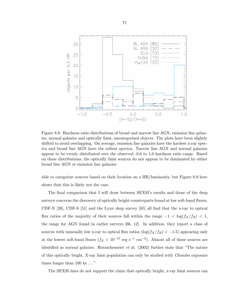
71

Figure 8.8: Hardness ratio distributions of broad and narrow line AGN, emission line galax-ies, normal galaxies and optically faint, uncategorized objects. The plots have been slightlyshifted to avoid overlapping. On average, emission line galaxies have the hardest x-ray spec-tra and broad line AGN have the softest spectra. Narrow line AGN and normal galaxiesappear to be evenly distributed over the observed -0.6 to 1.0 hardness ratio range. Basedon these distributions, the optically faint sources do not appear to be dominated by eitherbroad line AGN or emission line galaxies.

able to categorize sources based on their location on a HR/luminosity, but Figure 8.9 here

shows that this is likely not the case.

The final comparison that I will draw between SEXSI’s results and those of the deep

surveys concerns the discovery of optically bright counterparts found at low soft-band fluxes.

CDF-N [20], CDF-S [51] and the Lynx deep survey [65] all find that the x-ray to optical

flux ratios of the majority of their sources fall within the range −1 < log(fX/fR) < 1,

the range for AGN found in earlier surveys [66, 12]. In addition, they report a class of

sources with unusually low x-ray to optical flux ratios (log(fX/fR) < −1.5) appearing only

at the lowest soft-band fluxes (fX < 10−15 erg s−1 cm−2). Almost all of these sources are

identified as normal galaxies. Hornschemeier et al. (2002) further state that “The nature

of this optically bright, X-ray faint population can only be studied with Chandra exposure

times longer than 100 ks . . . ”

The SEXSI data do not support the claim that optically bright, x-ray faint sources can

72

Figure 8.9: Hardness ratio vs. soft-band (left) and hard-band (right) luminosities. Contraryto the results of the CDF-S, we find considerable overlap among the different categories ofsources. As in the case of HR vs. flux, we find that hardness increases with decreasingsoft-band luminosity, but that the correlation with hard-band luminosity is much weaker.

only be studied by deep-field observations. Figure 8.10 shows scatter plots of the hard

and soft-band x-ray flux to optical flux ratios vs. their respective x-ray band fluxes. In

the soft log(fX/fR) plot, we also find normal galaxies with low soft x-ray to optical flux

ratios. Those detected in the soft band (marked with a solid dot inside the plot symbols)

have fluxes between 4 × 10−16 and 10−14 erg s−1 cm−2. Included in this sample, but not

showing up in the soft-band plot, are sources detected only in the hard band (HR = 1).

In the hard-band plot, sources with fXsoft/fR < −1.5 are again denoted with solid dots

inside their plot symbols. As the deep surveys find, these sources are almost exclusively

emission-line galaxies, although a few early-type galaxies and narrow line AGN also ap-

pear. These sources are easily detected in the hard band, ranging in flux from 10−15 to

3 × 10−14 erg s−1 cm−2. CDF-S [61] also find a large number of hard-band only sources

which they do not comment on, regarding the optically bright/soft x-ray faint population.

In addition, the existence of this population should not be a surprise, given the results

of the Extended Medium Sensitivity Survey (EMSS) [66], where they identified optically

bright (−2 < log(fX/fV ) < −1) normal galaxies with soft-band fluxes of approximately

73

Figure 8.10: (a) Soft-band (0.5 – 2.1 keV) and (b) Hard-band (2.1 – 10.0 keV) x-ray tooptical (R band) flux ratios vs. the respective x-ray band flux. The dashed lines indicate linesof constant optical flux, at mR = 24 and mR = 25. In general, we do not spectroscopicallypursue sources with mR > 24. Sources with low soft x-ray to optical flux ratios (< −1.5)are marked with a solid dot. The Ms surveys only observe these sources at soft fluxesbelow 10−15 erg s−1 cm−2. SEXSI, and EMSS before, demonstrate that the optically brightgalaxies are not confined to low soft x-ray fluxes.

74

10−13 erg s−1 cm−2. In the EMSS, the source density of optically bright/soft x-ray faint

sources is low, only 0.015 sources per sq. degree at the EMSS flux limit. It is not surprising

that the deep surveys, which only cover 0.07 sq. degrees, would not detect the brighter (in

x-ray flux) of these optically bright soft sources.

The preliminary results of this survey have confirmed several of the results seen earlier

in the Ms surveys: the trend for fainter soft-band sources to have harder x-ray spectra and

the weak dependence of hardness ratio on hard-band flux, the preponderance of soft sources

in the broad line AGN distribution, and the trend for harder sources to appear at lower

redshifts. We differ from the results of the Ms surveys mainly in our identification of the

hard sources. Whereas the CDF-S finds mostly type 2 AGN at low redshifts and high HRs,

we find a combination of emission line galaxies, early-type galaxies and broad line AGN.

Deeper optical spectroscopy, however, may reveal AGN signatures in the sources that we

categorize as emission-line and early-type galaxies. CDF-S finds clear separation by source

type in the HR vs. luminosity plane while we find that there are significant areas of overlap

among the different classes of sources. Finally, we note that the optically bright but soft

x-ray faint population of sources found in the Ms surveys also exist at brighter soft fluxes

and, in fact, were detected a decade ago in the EMSS.

8.2.2 Emission line galaxies

Emission line galaxies (ELGs) form the second largest subpopulation in our survey, next to

the broad line AGN, yet the x-ray emission mechanism remains unknown. XRB synthesis

theories suppose that obscured AGN are the main contributors to hard x-ray flux, but the

star formation is known to produce x-ray emission, so starburst galaxies, those with star

formation rates (SFR) greater than 100 M/yr, must also be considered. Estimates of the

SFR from [Oii] luminosity indicates that star formation in SEXSI’s ELGs is not at the level

of starburst galaxies. Kennicutt (1998) [67] gives the following as an estimate of the SFR

in a galaxy from the [Oii] luminosity:

SFR(M yr−1) = (1.4 ± 0.4)× 10−41L[OII](erg s−1). (8.1)

Among the SEXSI ELGs, we find that the SFRs inferred from [Oii] luminosities range

from 0.5–10 M/yr, well below the rates of starburst galaxies. We can also estimate the

75

fraction of the x-ray emission that is due to star formation. Stern et al. (2002) [65] derive

an estimate of the SFR in starburst galaxies based on the 2–10 keV x-ray luminosity of a

source:

SFR(M yr−1) = (2− 20)× 10−40L2−10 keV(erg s−1). (8.2)

Figure 8.11 plots the fraction of x-ray luminosity from star formation vs. the SFR for the

SEXSI’s ELGs. The contribution to x-ray emission from star formation falls in the 10−5 –

10−3 range. The small fractions of x-ray luminosity that can be attributed to star formation

leaves open the strong likelihood that the bulk of the x-ray emission is produced by a heavily

obscured AGN.

Figure 8.11: Fractional contribution of x-ray emission due to star formation vs. star for-mation rate. The SFR is estimated from the [Oii]λ3727 luminosity using Equation 8.1 andthe 2–10 keV x-ray luminosity attributed to star formation is calculated from Equation 8.2.The range in the error bars correspond to the range in the conversion factor of Equation8.2.

8.3 The future of SEXSI

The results presented here only show the basic trends in the extragalactic x-ray source

population detected at 10−13 − 10−15 erg s−1 cm−2. The SEXSI survey samples the bright

76

end of the cumulative source distribution (logN − logS) with a far greater number of

sources than the Ms surveys have access to. We can obtain a much more accurate measure

of the logN − logS at the brighter fluxes and determine the field-to-field variability of that

distribution.

We can also use the data from SEXSI to investigate the nature of the x-ray emitting

normal galaxies. Arguably, some fraction of the x-ray emission from these galaxies comes

from starburst regions, but is there AGN activity buried within these galaxies? Composite

optical spectra of the normal galaxies may reveal weak AGN signatures, such as Mgii or

[Nev] but in order to maximize the signal to noise on these faint lines, we will need to

identify and set aside the spectra of galaxies with strong starburst signatures.

The x-ray data on most of the sources that we detect only consist of tens of photons. By

creating composite x-ray spectra from the existing detections, we may be able to measure

the average absorbing column for subsets of the population and determine the intrinsic

source spectrum. These results could strengthen the case for the unified model of AGN and

incorporate the emission-line and early-type galaxies that we observe into the unified model

as the most heavily obscured AGN.

77

Chapter 9 Conclusion

We have undertaken the two projects described in this thesis, HEFT and SEXSI, in order

to explore the x-ray universe at higher energies and to fainter fluxes. By observing hard

x-ray emission, we can study nonthermal emission mechanisms, such as inverse Compton

scattering galaxy clusters and nuclear decay lines from supernova remnants, and we can

study sources that are obscured at lower energies. The bulk of the x-ray emission in the

universe is believed to arise from the accretion that powers AGN; however, the discrepancy

between the integrated spectra of the local AGN population and that of the XRB leads us

to conclude that the bulk of the sources are heavily obscured and can only be detected at

higher energies. SEXSI is an effort to address this problem with the best instrumentation

currently available, the Chandra X-ray Observatory, and HEFT is an effort to extend the

sensitivity advantages of a focusing telescope into the hard x-ray band (10–100 keV).

HEFT’s first flight is currently scheduled for the fall of 2003. The balloon will be

launched from either Fort Sumner, NM, or Palestine, TX, and will remain at altitude (40

km) for up to 48 hours. For the first flight, we will have at least two telescope modules

assembled and integrated into the payload. The first two optics modules will use the W/Si

design described in this thesis. As the fabrication progresses, the coating designs will

change as we find better ways to optimize their design. One of the changes intended for

future modules will be Ni0.93V0.07/Si coatings for the inner shells. This will allow the HEFT

band to be extended from 70 keV up to 100 keV.

By 2005, all of HEFT 14 telescope modules will be complete and we will be able to take

advantage of results from Swift’s hard x-ray all-sky survey. Swift expects to find 400–600

x-ray sources in its milli-Crab sensitivity survey. In a 20 ks exposure, HEFT will be able

to measure the hard x-ray spectra of the faintest objects in the Swift survey. In addition,

with HEFT’s superior angular resolution (1′ vs. 17′ for Swift), we will be better equipped

to identify the hard x-ray sources in other wavelength bands.

Focusing instruments are well suited for deep field surveys, as Chandra has shown, but

HEFT’s sensitivity is insufficient to conduct deep surveys. The source density in the hard x-

rays is unknown, but extrapolating from the Swift estimate, a 100 ks random pointing with

78

HEFT would only have a 30% chance of detecting a single source. For the future, higher

sensitivity satellite-borne telescopes are being planned. NASA’s proposed Constellation-

X mission will have an effective area five times that of HEFT. Deep surveys by these

instruments will allow us to study x-ray sources that are obscured at soft x-ray energies

(< 10 keV).

Presently, however, the best available x-ray telescope for studying obscured sources is

the Chandra X-ray Observatory. The SEXSI survey complements the single pointing deep

Chandra surveys by covering a substantially larger area of the sky, but to a shallower

flux level. The larger sky coverage gives us excellent statistics on the bright end (∼> 10−15

erg cm−2 s−1) of the deep Chandra survey distribution, where they only find tens of sources.

Most of our results echo those of the deep surveys; the major difference we find is that the

optically bright sources that the deep surveys find at low soft-band flux also can be found

at higher soft-band fluxes and over a wide range in hard-band fluxes.

One of the mysteries raised by the SEXSI survey is the nature of the emission line

galaxies that we find in the Chandra hard band selected sample. These sources make up a

considerable fraction of the source population and are likely, give their strong x-ray fluxes,

to contain buried AGN. For now, we are looking for optical signatures of AGN activity in

these objects, but the definitive answer on the nature of these sources may have to wait

until we build the next generation of hard x-ray telescopes.

79

Bibliography

[1] Proposers Observatory Guide. TD 403.00.04, Chandra X-ray Center, December 2001.

[2] J. H. Hubbell and S. M. Seltzer. Tables of x-ray mass attenuation coefficients and

mass energy-absorption coefficients. Technical Report NISTIR 5632, web version 1.02,

NIST, http://physics.nist.gov/PhysRefData/XrayMassCoef/cover.html, 1997.

[3] R. Morrison and D. McCammon. Interstellar photoelectric absorption cross sections,

0.03-10 keV. Astrophys. J., 270:119–122, July 1983.

[4] F. E. Christensen, A. Hornstrup, N. J. Westergaard, H. W. Schnopper, J. L. Wood, and

K. Parker. A graded d-spacing multilayer telescope for high energy x-ray astronomy. In

Richard B. Hoover, editor, Multilayer and grazing incidence X-ray/EUV optics, volume

1546, pages 160–167. Proc. SPIE, 1992.

[5] K. D. Joensen, F. E. Christensen, H. W. Schnopper, P. Gorenstein, J. Susini, P. Hoghoj,

R. Hustache, J. L. Wood, and K. Parker. Medium-sized grazing incidence high-energy

x-ray telescopes employing continuously graded multilayers. In Richard B. Hoover,

editor, X-Ray Detector Physics and Applications, volume 1736, pages 239–248. Proc.

SPIE, 1993.

[6] K. Yamashita, P. J. Serlemitsos, J. Tueller, S. D. Barthelmy, L. M. Bartlett, K. W.

Chan, A. Furuzawa, N. Gehrels, K. Haga, H. Kunieda, P. Kurczynski, G. Lodha,

N. Nakajo, N. Nakamura, Y. Namba, Y. Ogasaka, T. Okajima, D. Palmer, A. Par-

sons, Y. Soong, S. M. Stahl, H. Takata, K. Tamura, Y. Tawara, and B. J. Teegarden.

Supermirror hard-x-ray telescope. Applied Optics, 37(34):8067–8073, 1998.

[7] P. H. Mao, F. A. Harrison, Y. Y. Platonov, D. Broadway, B. Degroot, F. E. Christensen,

W. W. Craig, and C. J. Hailey. Development of grazing incidence multilayer mirrors

for hard x-ray focusing telescopes. Proc. SPIE, 3114:526–534, October 1997.

80

[8] C. J. Hailey, S. Abdali, F. E. Christensen, W. W. Craig, T. R. Decker, F. A. Harrison,

and M. Jimenez-Garate. Substrates and mounting techniques for the High-Energy

Focusing Telescope (HEFT). Proc. SPIE, 3114:535–543, October 1997.

[9] H. Tananbaum, N. White, and P. Sullivan, editors. Proceedings of the High Throughput

X-ray Spectroscopy Workshop. Harvard-Smithsonian Center for Astrophysics, 1996.

[10] R. F. Mushotzky, C. Done, and K. A. Pounds. X-ray spectra and time variability of

active galactic nuclei. Annu. Rev. Astron. Astrophys., 31:717–761, 1993.

[11] G. Hasinger, R. Burg, R. Giacconi, M. Schmidt, J. Trumper, and G. Zamorani. The

ROSAT Deep Survey. I. X-ray sources in the Lockman Field. Astron. & Astrophys.,

329:482–494, January 1998.

[12] M. Schmidt, G. Hasinger, J. Gunn, D. Schneider, R. Burg, R. Giacconi, I. Lehmann,

J. MacKenty, J. Trumper, and G. Zamorani. The ROSAT deep survey. II. Optical

identification, photometry and spectra of X-ray sources in the Lockman field. Astron.

& Astrophys., 329:495–503, January 1998.

[13] G. Setti and L. Woltjer. Active Galactic Nuclei and the spectrum of the X-ray back-

ground. Astron. & Astrophys., 224:L21–L23, October 1989.

[14] P. Madau, G. Ghisellini, and A. C. Fabian. The Unified Seyfert Scheme and the Origin

of the Cosmic X-Ray Background. Mon. Not. R. Astron. Soc., 270:L17–+, September

1994.

[15] A. Comastri, G. Setti, G. Zamorani, and G. Hasinger. The contribution of AGNs to

the X-ray background. Astron. & Astrophys., 296:1+, April 1995.

[16] R. Gilli, M. Salvati, and G. Hasinger. Testing current synthesis models of the X-ray

background. Astron. & Astrophys., 366:407–417, February 2001.

[17] A. C. Fabian and X. Barcons. The origin of the X-ray background. Annu. Rev. Astron.

Astrophys., 30:429–456, 1992.

[18] A. C. Fabian. The obscured growth of massive black holes. Mon. Not. R. Astron. Soc.,

308:L39–L43, October 1999.

81

[19] R. F. Mushotzky, L. L. Cowie, A. J. Barger, and K. A. Arnaud. Resolving the extra-

galactic hard X-ray background. Nature, 404:459–464, March 2000.

[20] A. E. Hornschemeier, W. N. Brandt, G. P. Garmire, D. P. Schneider, A. J. Barger,

P. S. Broos, L. L. Cowie, L. K. Townsley, M. W. Bautz, D. N. Burrows, G. Chartas,

E. D. Feigelson, R. E. Griffiths, D. Lumb, J. A. Nousek, L. W. Ramsey, and W. L. W.

Sargent. The Chandra Deep Survey of the Hubble Deep Field-North Area. II. Results

from the Caltech Faint Field Galaxy Redshift Survey Area. Astrophys. J., 554:742–777,

June 2001.

[21] F. Fiore, F. La Franca, C. Vignali, A. Comastri, G. Matt, G. C. Perola, M. Cappi,

M. Elvis, and F. Nicastro. Spectroscopic identification of ten faint hard X-ray sources

discovered by Chandra. New Astronomy, 5:143–153, July 2000.

[22] A. Toor and F. D. Seward. The Crab Nebula as a calibration source for X-ray astron-

omy. Astron. J., 79:995–999, October 1974.

[23] A. M. Levine, F. L. Lang, W. H. G. Lewin, F. A. Primini, C. A. Dobson, J. P. Doty,

J. A. Hoffman, S. K. Howe, A. Scheepmaker, W. A. Wheaton, J. L. Matteson, W. A.

Baity, D. E. Gruber, F. K. Knight, P. L. Nolan, R. M. Pelling, R. E. Rothschild, and

L. E. Peterson. The HEAO 1 A-4 catalog of high-energy X-ray sources. Astrophys. J.

Suppl., 54:581–617, April 1984.

[24] Swift: hard x-ray survey. http://swift.gsfc.nasa.gov/scitech/science/survey.html.

[25] S. E. Woosley and R. D. Hoffman. Co-57 and Ti-44 production in SN 1987A. Astrophys.

J., 368:L31–L34, February 1991.

[26] F. A. Harrison, S. E. Boggs, A. E. Bolotnikov, C. M. H. Chen, W. R. Cook, and S. M.

Schindler. Development of CdZnTe pixel detectors for astrophysical applications. In

Proc. SPIE Vol. 4141, p. 137-143, Hard X-Ray, Gamma-Ray, and Neutron Detector

Physics II, Ralph B. James; Richard C. Schirato; Eds., volume 4141, pages 137–143,

November 2000.

[27] A. Snigirev, V. Kohn, I. Snigireva, and B. Lengeler. A compound refractive lens for

focusing high-energy x-rays. Nature, 384(6604):49–51, 1996.

82

[28] L. Nevot and P. Croce. Caracterisation des surfaces par reflexion rasante de rayons

x. application a l’etude du polissage de quelques verres silicates. Revue. Phys. Appl.,

15:761–779, 1980.

[29] E. Spiller. Soft X-ray Optics. SPIE Engineering Press, Bellingham, USA, 1994.

[30] F. Mezei. Novel polarized neutron devices: supermirror and spin component amplifier.

Comm. on Phys., 1:81–85, 1976.

[31] Karsten Dan Joensen. Design, Fabrication, and Characterization of Multilayers for

Broad-band, Hard X-ray Astrophysics Instrumentation. PhD thesis, University of

Copenhagen, 1995.

[32] J. Schelten and K. Mika. Calculated reflectivities of supermirrors. Nucl. Instrum. and

Meth., 160:287–294, 1978.

[33] J. B. Hayter and H. A. Mook. Discrete thin-film multilayer design for x-ray and neutron

supermirrors. Journal of Applied Crystallography, 22(1):35–41, 1989.

[34] S. Yamada, T. Ebisawa, N. Achiwa, T. Akiyoshi, and S. Okamoto. Neutron-optical

properties of multilayer systems. Annu. Rep. Res. Reactor Inst., 11:8–27, 1978.

[35] A. V. Tikhonravov. Synthesis of optical coatings using optimality conditions. Vestn.

Mosk. Univ. Fiz. Astronomiya, 23:91–93, 1982.

[36] A. N. Baskakov and A. V. Tikhonravov. Synthesis of two-component optical coatings.

Opt. Spectrosc., 56:915–919, 1984.

[37] I. V. Kozhevnikov, I. N. Bukreeva, and E. Ziegler. Theoretical study of multilayer x-ray

mirrors with a wide spectral band of reflection. Proc. SPIE, 3448:322–331, December

1998.

[38] I. V. Kozhevnikov, I. N. Bukreeva, and E. Ziegler. Design of x-ray supermirrors. Nucl.

Instr. and Meth. A, 460:424–443, 2001.

[39] A. G. Michette and Z. Wang. Optimisation of depth-graded multilayer coatings for

broadband reflectivity in the soft X-ray and EUV regions. Optics Communications,

177:47–55, April 2000.

83

[40] K. Yamashita, H. Kunieda, Y. Tawara, K. Tamura, Y. Ogasaka, K. Haga, T. Okajima,

Y. Hidaka, S. Ichimaru, S. Takahashi, A. Goto, H. Kito, Y. Tsusaka, K. Yokoyama,

and S. Takeda. New design concept of multilayer supermirrors for hard x-ray optics.

Proc. SPIE, 3766:327–335, September 1999.

[41] V. V. Protopopov, A. V. Tikhonravov, A. V. Voronov, M. K. Trubetskov, and G. W.

Debell. Optimal design of graded x-ray multilayer mirrors in the angular and spectral

domains. Proc. SPIE, 3766:320–326, September 1999.

[42] P. H. Mao, F. A. Harrison, D. L. Windt, and F. E. Christensen. Optimization of graded

multilayer designs for astronomical x-ray telescopes. Appl. Opt., 38:4766–4775, August

1999.

[43] W. H. Press, B. P. Flannery, S. A. Teukolsky, and W. T. Vetterling. Numerical Recipes

in C. Cambridge University Press, New York, 1988.

[44] J. A. Nelder and R. Mead. Computer Journal, 7:308–313, 1965.

[45] PXRMS multilayer survey results. http://www-cxro.lbl.gov/cgi-bin/mldata.pl.

[46] J. L. Vossen and W. Kern. Thin Film Processes. Academic Press, 1978.

[47] D. L. Windt. Periodic and depth-graded cu/si multilayer films for hard x-ray optics.

Applied Physics Letters, 74(19):2890–2892, 1999.

[48] D. L. Windt and W. K. Waskiewicz. Multilayer facilities required for extreme-

ultraviolet lithography. J. Vac. Sci. Technol B, 12(6):3826–3832, 1994.

[49] F. E. Christensen, W. W. Craig, D. L. Windt, M. A. Jimenez-Garate, C. J. Hailey,

F. A. Harrison, P. H. Mao, J. M. Chakan, E. Ziegler, and V. Honkimaki. Measured

reflectance of graded multilayer mirrors designed for astronomical hard x-ray telescopes.

NIM-A, 451(3):572–581, 2000.

[50] W. W. Craig, C. J. Hailey, M. Jimenez-Garate, D. L. Windt, F. A. Harrison, P. H.

Mao, F. E. Christensen, and A. M. Hussain. Development of thermally formed glass

optics for astronomical hard x-ray telescopes. Optics Express, 7(4):178–185, 2000.

84

[51] R. Giacconi, P. Rosati, P. Tozzi, M. Nonino, G. Hasinger, C. Norman, J. Bergeron,

S. Borgani, R. Gilli, R. Gilmozzi, and W. Zheng. First Results from the X-Ray and

Optical Survey of the Chandra Deep Field South. Astrophys. J., 551:624–634, April

2001.

[52] P. Rosati, P. Tozzi, R. Giacconi, R. Gilli, G. Hasinger, L. Kewley, V. Mainieri, M. Non-

ino, C. Norman, G. Szokoly, J. X. Wang, A. Zirm, J. Bergeron, S. Borgani, R. Gilmozzi,

N. Grogin, A. Koekemoer, E. Schreier, and W. Zheng. The Chandra Deep Field-South:

The 1 Million Second Exposure. Astrophys. J., 566:667–674, February 2002.

[53] The ASCA Data Reduction Guide.

http://heasarc.gsfc.nasa.gov/docs/asca/abc/abc.html.

[54] W. N. Brandt, D. M. Alexander, A. E. Hornschemeier, G. P. Garmire, D. P. Schneider,

A. J. Barger, F. E. Bauer, P. S. Broos, L. L. Cowie, L. K. Townsley, D. N. Burrows,

G. Chartas, E. D. Feigelson, R. E. Griffiths, J. A. Nousek, and W. L. W. Sargent. The

Chandra Deep Field North Survey. V. 1 Ms Source Catalogs. Astron. J., 122:2810–2832,

December 2001.

[55] J. B. Oke, J. G. Cohen, M. Carr, J. Cromer, A. Dingizian, F. H. Harris, S. Labrecque,

R. Lucinio, W. Schaal, H. Epps, and J. Miller. The Keck Low-Resolution Imaging

Spectrometer. Proc. Astron. Soc. Pacific, 107:375+, April 1995.

[56] P. Massey. A User’s Guide to CCD Reductions with IRAF.

http://iraf.noao.edu/iraf/ftp/iraf/docs/ccduser3.ps.Z, 1997.

[57] A. U. Landolt. UBVRI photometric standard stars in the magnitude range 11.5-16.0

around the celestial equator. Astron. J., 104:340–371, July 1992.

[58] P. Massey, F. Valdes, and J. Barnes. A User’s Guide to Reducing Slit Spectra with

IRAF. http://iraf.noao.edu/iraf/ftp/iraf/docs/spect.ps.Z, 1992.

[59] J. B. Oke and J. E. Gunn. Secondary standard stars for absolute spectrophotometry.

Astrophys. J., 266:713–717, March 1983.

[60] P. Massey and C. Gronwall. The Kitt Peak spectrophotometric standards - Extension

to 1 micron. Astrophys. J., 358:344–349, July 1990.

85

[61] P. Tozzi, P. Rosati, M. Nonino, J. Bergeron, S. Borgani, R. Gilli, R. Gilmozzi,

G. Hasinger, N. Grogin, L. Kewley, A. Koekemoer, C. Norman, E. Schreier, G. Szokoly,

J. X. Wang, W. Zheng, A. Zirm, and R. Giacconi. New Results from the X-Ray and

Optical Survey of the Chandra Deep Field-South: The 300 Kilosecond Exposure. II.

Astrophys. J., 562:42–51, November 2001.

[62] M. J. Page, J. P. D. Mittaz, and F. J. Carrera. A survey of hard spectrum ROSAT

sources - II. Optical identification of hard sources. Mon. Not. R. Astron. Soc., 325:575–

583, August 2001.

[63] R. E. Griffiths, R. della Ceca, I. Georgantopoulos, B. J. Boyle, G. C. Stewart,

T. Shanks, and A. Fruscione. A Deep ROSAT Survey – X. X-ray-luminous narrow-

emission-line galaxies. Mon. Not. R. Astron. Soc., 281:71–83, July 1996.

[64] I. M. McHardy, L. R. Jones, M. R. Merrifield, K. O. Mason, A. M. Newsam, R. G.

Abraham, G. B. Dalton, F. Carrera, P. J. Smith, M. Rowan-Robinson, and R. G.

Abraham. The origin of the cosmic soft X-ray background – Optical identification of

an extremely deep ROSAT survey. Mon. Not. R. Astron. Soc., 295:641+, April 1998.

[65] Daniel Stern et al. Spices ii: Optical and near-infrared identifications of faint x-ray

sources from deep Chandra observations of Lynx. Astrophys. J., 123(5):in press, 2002.

[66] J. T. Stocke, S. L. Morris, I. M. Gioia, T. Maccacaro, R. Schild, A. Wolter, T. A.

Fleming, and J. P. Henry. The Einstein Observatory Extended Medium-Sensitivity

Survey. II - The optical identifications. Astrophys. J. Suppl., 76:813–874, July 1991.

[67] R. C. Kennicutt. Star Formation in Galaxies Along the Hubble Sequence. Annu. Rev.

Astron. Astrophys., 36:189–232, 1998.

86

Appendix A HEFT optimization results

The following plots summarize the results of the HEFT optimization described in Chapter 4.

The program increments the number of layers by a factor of 1.25 at each step in the opti-

mization and terminates when the figure of merit drops from the previous step. The estimate

of the optimum is the second thickest coating. The dotted lines in each plot indicate figures

of merit 98% and 95% of the optimum value.

Figure A.1: Mirror group 1: 1.67 < α < 1.86.

87

Figure A.2: Mirror group 2: 1.86 < α < 1.86.

Figure A.3: Mirror group 3: 2.08 < α < 2.32.

88

Figure A.4: Mirror group 4: 2.32 < α < 2.59.

Figure A.5: Mirror group 5: 2.59 < α < 2.89.

89

Figure A.6: Mirror group 6: 2.89 < α < 3.22.

Figure A.7: Mirror group 7: 3.22 < α < 3.60.

90

Figure A.8: Mirror group 8: 3.60 < α < 4.01.

Figure A.9: Mirror group 9: 4.01 < α < 4.48.

91

Figure A.10: Mirror group 10: 4.48 < α < 5.00.

Who cares? It’s only a thesis.

—Fiona A. Harrison (1993)