harmonic analysis: from fourier to haarcrisp/courses/wavelets/fall09/chap1.pdf · harmonic...

Harmonic Analysis: from Fourier to Haar

Marıa Cristina Pereyra

Lesley A. Ward

Department of Mathematics and Statistics, MSC03 2150, 1 Univer-sity of New Mexico, Albuquerque, NM 87131-0001, USA

E-mail address: [email protected]

School of Mathematics and Statistics, University of South Aus-tralia, Mawson Lakes SA 5095, Australia

E-mail address: [email protected]

2000 Mathematics Subject Classification. Primary 42-xx

Contents

Introduction xv

Chapter 1. Fourier series: some motivation 11.1. Some examples and key definitions 11.2. Main questions 51.3. Fourier series and Fourier coefficients 71.4. A little history, and motivation from the physical world 11

Chapter 2. Interlude 172.1. Nested classes of functions on bounded intervals 172.2. Modes of convergence 282.3. Interchanging limit operations 342.4. Density 38

Chapter 3. Pointwise convergence of Fourier series 413.1. Pointwise convergence: why do we care? 413.2. Smoothness vs convergence 443.3. A suite of convergence theorems 50

Chapter 4. Summability methods: Dirichlet kernels and Fejer kernels 554.1. Partial Fourier sums and the Dirichlet kernel DN 554.2. Properties of the Dirichlet kernel 574.3. Convolution 594.4. Good kernels, or approximations of the identity 674.5. Fejer kernels and Cesaro means 724.6. Poisson kernels and Abel means 754.7. Excursion into Lp(T) 76

Chapter 5. Mean-square convergence of Fourier series 795.1. Basic Fourier theorems in L2(T) 795.2. Geometry of the Hilbert space L2(T) 815.3. Completeness of the trigonometric system 855.4. Equivalent conditions for completeness in L2(T) 90

Chapter 6. A whirlwind tour of discrete Fourier and Haar analysis 956.1. Fourier Series: a summary 956.2. The discrete Fourier basis 966.3. A parenthesis on bases and dual bases in CN 1006.4. The discrete Fourier transform and its inverse 1016.5. The Fast Fourier Transform (FFT) 1026.6. The discrete Haar basis 107

v

vi CONTENTS

6.7. The Discrete Haar Transform 1106.8. The Fast Haar Transform 111

Chapter 7. The Fourier transform in paradise 1157.1. From Fourier series to Fourier integrals 1167.2. The Fourier transform on the Schwartz class S(R) 1177.3. The time–frequency dictionary for S(R) 1197.4. The Schwartz class is closed under the Fourier transform 1227.5. Convolution and approximations of the identity on R 1257.6. An interlude on kernels 1287.7. The Fourier Inversion Formula, and Plancherel’s Identity 1307.8. Lp-norms on S(R) 133

Chapter 8. Beyond paradise 1378.1. Functions of moderate decrease 1378.2. Tempered distributions 1408.3. The time–frequency dictionary for S ′(R) 1438.4. The delta distribution 1478.5. Some applications of the Fourier transform 1498.6. Lp(R) as distributions 155

Chapter 9. From Fourier to Haar 1619.1. The windowed Fourier transform, and Gabor bases 1619.2. The wavelet transform 1659.3. Haar analysis 1679.4. Haar vs Fourier 1819.5. Unconditional bases, martingale transforms, and square functions 183

Chapter 10. Zooming properties of wavelets, and applications 18510.1. Multiresolution analyses (MRAs) 18510.2. The Haar multiresolution analysis 18710.3. From MRA to wavelets: Mallat’s Theorem 19210.4. Mallat’s algorithm revisited 19710.5. Cascade algorithm and filter banks 20010.6. Design features 20410.7. A catalog of wavelets 20610.8. Wavelet packets 20710.9. Two-dimensional wavelets 20910.10. Basics of compression and denoising 210

Chapter 11. The Hilbert transform 21311.1. The Hilbert transform on the frequency domain: Fourier multipliers 21311.2. The Hilbert transform on the time domain: singular integrals 21511.3. Boundedness properties of the Hilbert transform 21711.4. The function space weak-L1(R) 22011.5. Interpolation theorems 22811.6. A festival of inequalities 23311.7. Some history to conclude our journey 23911.8. Disclaimer 244

CONTENTS vii

Chapter 12. Projects for students 24512.1. Fourier analysis on finite groups 24612.2. Two extremal problems on curves 24912.3. Weyl’s equidistribution theorem 24912.4. The Gibbs phenomenon for Fourier series and for wavelets 25012.5. Linear and nonlinear approximation in Fourier and Haar bases 25212.6. Monsters 25312.7. The power of averaging or summability methods 25512.8. Local cosine and sine bases 25712.9. The twin dragon and fractals in wavelets 25712.10. Fourier analysis and wavelets on graphs 25812.11. The discrete and finite Hilbert transforms and Cotlar’s Lemma 25912.12. Edge Detection 26012.13. The Hilbert transform of characteristic functions 26112.14. The Calderon–Zygmund decomposition and weak-L1 estimates 26212.15. BMO, John-Nirenberg and Stopping time 26612.16. The Hilbert transform as an average of Haar multipliers 268

Appendix A. Some useful facts from analysis 271

Appendix B. Vector spaces, norms, inner products 273B.1. Vector spaces 273B.2. Normed spaces 274B.3. Inner-product vector spaces 274

Bibliography 281

CHAPTER 1

Fourier series: some motivation

In this book we discuss three types of Fourier analysis: first, Fourier series,in which the input is a periodic function on R, and the output is a two-sidedseries where the summation is over n ∈ Z; second, finite Fourier analysis, wherethe input is a vector of length N with complex entries, and the output is anothervector in CN ; and third, the Fourier transform, where the input is a function on R,and the output is another function on R.

As an aside, we note that one can also do Fourier analysis on Rn, on abeliangroups, on graphs, and in still more abstract settings. See [SS1, Chapter 7]. Fourieranalysis is also connected with representation theory. Some of the projects inChapter 12 are related to these abstract settings.

1.1. Some examples and key definitions

The central idea of Fourier analysis is to break a function into a combination ofsimpler functions. We think of these simpler functions as building blocks. We willalso be interested in reconstructing the original function from the building blocks.Here is a colorful analogy: a prism or raindrop can break a ray of (white) light intoall colors of the rainbow. The analogy is quite apt: the different colors correspondto different wavelengths/frequencies of light. We will see that our simpler functionscan also correspond to pure frequencies. For example, we will shortly consider sineand cosine functions of various frequencies as our first example of building blocks.When played aloud, a given sine or cosine function produces a pure tone, or note,or harmonic, at a single frequency. The term harmonic analysis evokes this idea ofseparation of a sound, or in our terms a function, into pure tones.

Expressing a function as a combination of building blocks is also called decom-posing the function. In Chapters 9 and 10 we will study so-called time–frequencydecompositions, in which each building block encodes information about time aswell as about frequency, very much like musical notation does.

We begin with an example.

Example 1.1. (Toy Model of Voice Signal) Suppose Amanda is in Baltimore,and she calls her mother in Vancouver, saying ‘Hi Mom, it’s Amanda, and I can’twait to tell you what happened today’. What happens to the sound? As Amandaspeaks, she creates waves of pressure in the air, which travel toward the phonereceiver. The sound has duration, say about five seconds in this example, andintensity or loudness, which varies over time. It also has many other qualities thatmake it sound like speech rather than music, say. The sound of Amanda’s voicebecomes a signal, which travels along the phone wire or via satellite, and at theother end is converted back into a recognizable voice.

1

2 1. FOURIER SERIES: SOME MOTIVATION

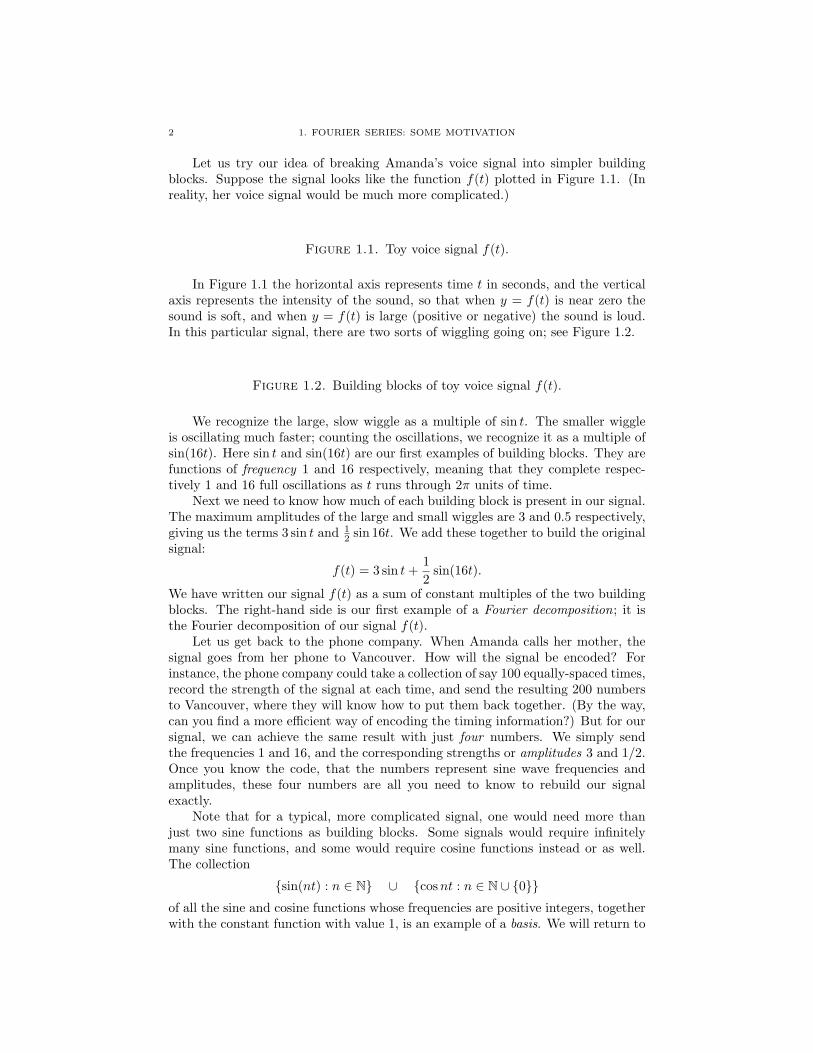
Let us try our idea of breaking Amanda’s voice signal into simpler buildingblocks. Suppose the signal looks like the function f(t) plotted in Figure 1.1. (Inreality, her voice signal would be much more complicated.)

Figure 1.1. Toy voice signal f(t).

In Figure 1.1 the horizontal axis represents time t in seconds, and the verticalaxis represents the intensity of the sound, so that when y = f(t) is near zero thesound is soft, and when y = f(t) is large (positive or negative) the sound is loud.In this particular signal, there are two sorts of wiggling going on; see Figure 1.2.

Figure 1.2. Building blocks of toy voice signal f(t).

We recognize the large, slow wiggle as a multiple of sin t. The smaller wiggleis oscillating much faster; counting the oscillations, we recognize it as a multiple ofsin(16t). Here sin t and sin(16t) are our first examples of building blocks. They arefunctions of frequency 1 and 16 respectively, meaning that they complete respec-tively 1 and 16 full oscillations as t runs through 2π units of time.

Next we need to know how much of each building block is present in our signal.The maximum amplitudes of the large and small wiggles are 3 and 0.5 respectively,giving us the terms 3 sin t and 1

2 sin 16t. We add these together to build the originalsignal:

f(t) = 3 sin t+12

sin(16t).

We have written our signal f(t) as a sum of constant multiples of the two buildingblocks. The right-hand side is our first example of a Fourier decomposition; it isthe Fourier decomposition of our signal f(t).

Let us get back to the phone company. When Amanda calls her mother, thesignal goes from her phone to Vancouver. How will the signal be encoded? Forinstance, the phone company could take a collection of say 100 equally-spaced times,record the strength of the signal at each time, and send the resulting 200 numbersto Vancouver, where they will know how to put them back together. (By the way,can you find a more efficient way of encoding the timing information?) But for oursignal, we can achieve the same result with just four numbers. We simply sendthe frequencies 1 and 16, and the corresponding strengths or amplitudes 3 and 1/2.Once you know the code, that the numbers represent sine wave frequencies andamplitudes, these four numbers are all you need to know to rebuild our signalexactly.

Note that for a typical, more complicated signal, one would need more thanjust two sine functions as building blocks. Some signals would require infinitelymany sine functions, and some would require cosine functions instead or as well.The collection

{sin(nt) : n ∈ N} ∪ {cosnt : n ∈ N ∪ {0}}of all the sine and cosine functions whose frequencies are positive integers, togetherwith the constant function with value 1, is an example of a basis. We will return to

1.1. SOME EXAMPLES AND KEY DEFINITIONS 3

Figure 1.3. Plot of an actual voice saying ‘Hi Mom, it’s Amanda,and I can’t wait to tell you what happened today’. Explain theunits: time in seconds along the horizontal axis, a proxy for vol-ume/intensity along the vertical axis. Check how long it lasts andcorrect the estimate (currently ‘five seconds’) in the first paragraphof this example.

the idea of a basis later; informally, it means a given collection of building blocksthat is able to express every function in some given class. Fourier series use sinesand cosines; other types of functions can be used as building blocks, notably in thewavelet series we will see later (Chapters 9 and 10).

Now let us be more ambitious. Are we willing to sacrifice a bit of the qualityof Amanda’s signal in order to send it more cheaply? Maybe. For instance, in oursignal the strongest component is the big wiggle. What if we send only the singlefrequency 1 and its corresponding amplitude 3? In Vancouver, only the big wigglewill be reconstructed, and the small fast wiggle will be lost from our signal. ButAmanda’s mother knows the sound of Amanda’s voice, and the imperfect recon-structed signal may still be recognizable. This is our first example of compressionof a signal.

To sum up: We analyzed our signal f(t), determining which building blockswere present and with what strength. We compressed the signal, discarding someof the frequencies and their amplitudes. We transmitted the remaining frequenciesand amplitudes. (At this stage we could also have stored the signal.) At the otherend they reconstructed the compressed signal.

Again, in practice one wants the reconstructed signal to be similar to the orig-inal signal. There are many interesting questions about which building blocks, andhow many, can be thrown away while retaining a recognizable signal. This is partof the subject of signal processing, in electrical engineering.

In the interests of realism, Figure 1.3 shows a plot of an actual voice saying ‘HiMom, it’s Amanda, and I can’t wait to tell you what happened today’. ♦

In another analogy, we can think of the decomposition as a recipe. The buildingblocks, distinguished by their frequencies, correspond to the different ingredients inyour recipe. You also need to know how much sugar, flour, and so on you have toadd to the mix to get your cake f ; that information is encoded in the amplitudesor coefficients.

The function f in Example 1.1 is especially simple. The intuition that sinesand cosines were sufficient to describe many different functions was gained from theexperience of the pioneers of Fourier analysis with physical problems (for instanceheat diffusion and the vibrating string) in the early eighteenth century; see Sec-tion 1.4. This intuition leads to the idea of expressing a periodic function f(θ) as


an infinite linear combination of sines and cosines, also known as a trigonometricseries:

(1.1) f(θ) ∼∞∑n=0

[bn sin(nθ) + cn cos(nθ)] .

We use the symbol ∼ to indicate that the right-hand side is the trigonometricseries associated with f . We don’t use the symbol = here since in some cases theleft- and right-hand sides of (1.1) are not equal, as discussed below.

We can rewrite the right-hand side of (1.1) as a linear combination of expo-nential functions. To do so, we use Euler’s Formula1: eiθ = cos θ + i sin θ, and thecorresponding formulas for sine and cosine in terms of exponentials, applied to nθfor each n,

cos θ =eiθ + e−iθ

2, sin θ =

eiθ − e−iθ

2i.

We will use the following version throughout:

(1.2) f(θ) ∼∞∑

n=−∞ane

inθ.

The right-hand side is called the Fourier series of f . We also say that f canbe expanded in a Fourier series. The coefficient an is called the nth Fourier co-efficient of f , and is often denoted by f (n) to emphasize the dependence on thefunction f . The coefficients {an} are determined by the coefficients {bn} and {cn}in the sine/cosine expansion.

Exercise 1.2. Write an in terms of bn and cn. ♦

1.2. Main questions

Our brief sketch immediately suggests several questions.• How can we find the Fourier coefficients an from the corresponding func-

tion f?• Given the {an}, how can we reconstruct f?• In what sense does the Fourier series converge? Pointwise? Uniformly?

Or in some other sense? If it does converge in some sense, how fast doesit converge?

• When the Fourier series does converge, is its limit equal to the originalfunction f?

• Which functions can we express with a trigonometric series∞∑

n=−∞ane

inθ ?

For example, must f be continuous, or Riemann integrable?

1This formula is named after the Swiss mathematician Leonhard Euler (pronounced “oiler”),

(1707–1783). We assume the reader is familiar with basic complex number operations andnotation. For example if v = a + ib, w = c + id, then v + w = (a + c) + i(b + d) and

vw = (ac − bd) + i(bc + ad). The algebra is done as it would be for real numbers, with the

extra fact that the imaginary unit i has the property that i2 = −1. The absolute value of acomplex number v = a+ ib is defined to be |v| =

√a2 + b2. See [Tao2, Section 15.6] for a quick

review of complex numbers.

1.2. MAIN QUESTIONS 5

• What other building blocks could we use besides sines and cosines, orequivalently exponentials?

We develop answers to these questions in the following pages, but before do-ing that let us compare to the more familiar problem of power series expansions.An infinitely-often differentiable function f can be expanded into a Taylor series2

centered say at x = 0,

(1.3) Taylor series and coefficients:∞∑n=0

cn xn, where cn =

f (n)(0)n!

.

The Taylor series always converges to f(0) = c0 when evaluated at x = 0. In the18th century mathematicians discovered that the traditional functions of calculus(sinx, cosx, ln(1 + x),

√1 + x, ex, etc.) can be expanded in Taylor series, and

that for these examples the Taylor series converges to the function in an openinterval containing x = 0, and they were very good at manipulating power seriesand calculating with them. That led them to believe that the same would be truefor all functions, which at the time meant infinitely-often differentiable functions.That dream was shattered by Cauchy’s3 discovery in 1821 of a counterexample.

Example 1.3. (Cauchy’s Counterexample) The function

f(x) =

{e−1/x2

, if x 6= 0;0, if x = 0

is infinitely often differentiable at every x, and f (n)(0) = 0 for all n ≥ 0. Thus itsTaylor series is identically equal to zero. Therefore the Taylor series will convergeto f(x) only for x = 0. ♦

Exercise 1.4. Verify that Cauchy’s function is infinitely differentiable. Con-centrate on what happens at x = 0. ♦

The Taylor polynomial of order N of a function f that can be differentiated atleast N times is given by the formula

(1.4) PN (f, 0) = f(0) + f ′(0)x+f ′′(0)

2!x2 + · · ·+ f (N)(0)

N !xN .

Exercise 1.5. Verify that if f is a polynomial of order less than or equal to N ,then f coincides with its Taylor polynomial of order N . ♦

Definition 1.6. A trigonometric4 polynomial of degree M is a function of theform

f(θ) =M∑

n=−Mane

inθ,

where an ∈ C for n = −M , . . . , M .

2Named after the English mathematician Brook Taylor (1685–1731). Sometimes the Taylorseries centered at x = 0 is called the Maclaurin series, named after the Scottish mathematicianColin Maclaurin (1698–1746).

3The French mathematician Augustin Louis Cauchy (1789–1857).4To be more precise, this particular trigonometric polynomial is 2π-periodic; see Section 1.3.1.


Exercise 1.7. Verify that if f is a trigonometric polynomial then its coeffi-cients {an} can be calculated with the following formula:

an =1

2π

∫ π

−πf(θ)e−inθ dθ.

♦

In both the Fourier and Taylor series, the problem is how well and in whatsense we can approximate a given function by using its Taylor polynomials (veryspecific polynomials) or by using its partial Fourier sums (very specific trigonomet-ric polynomials).

1.3. Fourier series and Fourier coefficients

We begin to answer our questions. The Fourier coefficients f(n) = an arecalculated using the formula suggested by Exercise 1.7:

(1.5) f(n) = an :=1

2π

∫ π

−πf(θ)e−inθ dθ.

Aside 1.8. The notation := indicates that we are defining the term on the leftof the :=, in this case an. Occasionally we may need to use =: instead, when weare defining a quantity on the right, as in Theorem 3.6 below.

One way to explain the appearance of formula (1.5) is to assume that thefunction f is equal to a trigonometric series,

f(θ) =∞∑

n=−∞ane

inθ,

and then to proceed formally5, operating on both sides of the equation. Multiplyboth sides by an exponential function, and then integrate, taking the liberty ofinterchanging the sum and the integral:

12π

∫ π

−πf(θ)e−ikθ dθ =

12π

∫ π

−π

∞∑n=−∞

aneinθe−ikθ dθ

=∞∑

n=−∞an

12π

∫ π

−πeinθe−ikθ dθ = ak.

The last equality holds because

(1.6)1

2π

∫ π

−πeinθe−ikθ dθ =

12π

∫ π

−πei(n−k)θ dθ = δn,k,

where the Kronecker6 delta δn,k is defined by

(1.7) δn,k =

{1, if k = n;0, if k 6= n.

5Here the term formally means that we work through a computation ‘following our noses’,without stopping to justify every step. In this example we don’t worry about whether the integrals

or series converge, or whether it is valid to exchange the order of the sum and the integral.A rigorous justification of our computation could start from the observation that it is valid to

exchange the sum and the integral if the Fourier series converges uniformly to f (see Chapters 2

and 4 for some definitions). Formal computations are often extremely helpful in building intuition.6Named after Leopold Kronecker, German mathematician and logician (1823–1891).

1.3. FOURIER SERIES AND FOURIER COEFFICIENTS 7

We explore the geometric meaning of equation (1.6) in Chapter 5. In languagewe will meet there, the equation says that the exponential functions {einx}n∈N forman orthonormal set.

Aside 1.9. The usual rules of calculus apply to complex-valued functions. Forexample, if u and v are the real and imaginary parts of the function f : [a, b]→ C,that is f = u+ iv where u and v are real-valued, then f ′ := u′ + iv′. Likewise, forintegration,

∫f =

∫u+ i

∫v. Here we are assuming that the functions u and v are

differentiable in the first case, and integrable in the second.

Notice that a necessary condition on f for the integral in formula (1.5) for thecoefficients to exist is that the complex-valued function f(θ)e−inθ should be anintegrable7 function on [−π, π). In fact, if |f | is integrable, then so is f(θ)e−inθ and

|an| =∣∣∣∣ 12π

∫ π

−πf(θ)e−inθ dθ

∣∣∣∣≤ 1

2π

∫ π

−π|f(θ)e−inθ| dθ (since

∣∣∫ g∣∣ ≤ ∫ |g|)=

12π

∫ π

−π|f(θ)| dθ (since |e−inθ| = 1)

<∞ (since f is integrable).

Aside 1.10. It can be verified that the absolute value of the integral of an in-tegrable complex-valued function is less than or equal to the integral of the absolutevalue of the function, the so-called triangle inequality for integrals, not to be con-fused with the triangle inequality for complex numbers: |a + b| ≤ |a| + |b|, or thetriangle inequality for integrable functions:

∫|f + g| ≤

∫|f | +

∫|g|. They are all

animals in the same family.

We now explore in what sense the Fourier series (1.2) approximates the originalfunction f . We begin with some examples.

Exercise 1.11. Find the Fourier coefficients and the Fourier series for thetrigonometric polynomial

f(θ) = 3e−2iθ − e−iθ + 1 + eiθ − πe4iθ +12e7iθ.

♦

Example 1.12. (Periodic Ramp Function) Compute the Fourier coefficientsand the Fourier series for the function

f(θ) = θ, for −π ≤ θ < π.

7A function g(θ) is said to be integrable on [−π, π) ifR π−π g(θ) dθ is well-defined; in particular

the value of the integral is a finite number. In harmonic analysis the notion of integral used is the

Lebesgue integral. We expect the reader to be familiar with Riemann-integrable functions meaningthat the function g is bounded and the integral exists in the sense of Riemann. Riemann-integrable

functions are Lebesgue integrable. In Chapter 2 we will briefly review the Riemann integral. See

[Tao1, Chapters 11], [Tao2, Chapters 19].These integration methods are named after the French mathematician Henri Lebesgue (1875–

1941), and the German mathematician Georg Friedrich Bernhard Riemann (1826–1866).


The nth Fourier coefficient is given by

f (n) = an :=1

2π

∫ π

−πf(θ)e−inθ dθ

=1

2π

∫ π

−πθe−inθ dθ

=

{(−1)n+1/(in), if n 6= 0;0, if n = 0.

using integration by parts in the last line. Thus the Fourier series of f(θ) = θ isgiven by

f(θ) ∼∑

{n∈Z:n 6=0}

(−1)n+1

ineinθ = 2

∞∑n=1

(−1)n+1

nsin (nθ).

Note that both f and its Fourier series are odd functions. It turns out that thefunction and the series coincide for all θ ∈ (−π, π). At the endpoints θ = ±πthe series converges to zero (the midpoint of the jump), since sin (nπ) = 0 for alln ∈ N. Notice that in this example the function and the series do not coincide atthe endpoints where the jump discontinuity occurs. ♦

Exercise 1.13. Fill in the details in the integration-by-parts argument in thecalculation in Example 1.12. ♦

1.3.1. 2π-Periodic functions. Note that we are considering functions

f : [−π, π)→ C

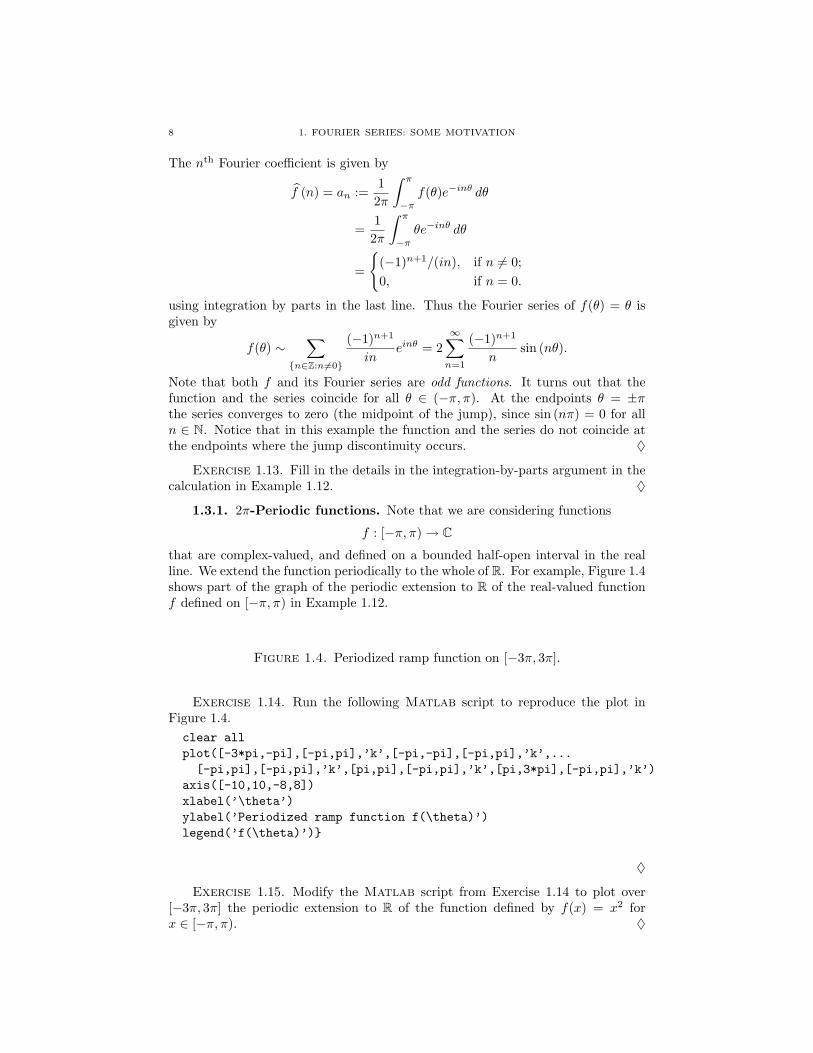
that are complex-valued, and defined on a bounded half-open interval in the realline. We extend the function periodically to the whole of R. For example, Figure 1.4shows part of the graph of the periodic extension to R of the real-valued functionf defined on [−π, π) in Example 1.12.

Figure 1.4. Periodized ramp function on [−3π, 3π].

Exercise 1.14. Run the following Matlab script to reproduce the plot inFigure 1.4.clear allplot([-3*pi,-pi],[-pi,pi],’k’,[-pi,-pi],[-pi,pi],’k’,...[-pi,pi],[-pi,pi],’k’,[pi,pi],[-pi,pi],’k’,[pi,3*pi],[-pi,pi],’k’)

axis([-10,10,-8,8])xlabel(’\theta’)ylabel(’Periodized ramp function f(\theta)’)legend(’f(\theta)’)}

♦

Exercise 1.15. Modify the Matlab script from Exercise 1.14 to plot over[−3π, 3π] the periodic extension to R of the function defined by f(x) = x2 forx ∈ [−π, π). ♦

1.3. FOURIER SERIES AND FOURIER COEFFICIENTS 9

In mathematical language, a function defined on R is 2π-periodic if f(x+2π) =f(x) for all x ∈ R. The building blocks we are using are 2π-periodic functions:sin(nθ), cos(nθ), e−inθ. Finite linear combinations of 2π-periodic functions are2π-periodic.

Let T denote the unit circle:

(1.8) T := {z ∈ C : |z| = 1} = {z = eiθ : −π ≤ θ < π}.We can identify a 2π-periodic function f on R with a function g : T → C

defined on the unit circle T as follows. Given z ∈ T there is a unique θ ∈ [−π, π)such that z = eiθ. Define

g(z) := f(θ).Note that if g is to be continuous on the unit circle T, we will need f(−π) =f(π). When we say f : T → C and f ∈ Ck(T), we mean that the function f isdifferentiable k times, and that f , f ′, . . . , f (k) are all continuous functions on T. Inwords, f is a k times continuously differentiable function from the unit circle intothe complex plane. In particular f (`)(−π) = f (`)(π) for all 0 ≤ ` ≤ k.

Note that if f is a 2π-periodic and integrable function, then the integral of fover each interval of length 2π takes the same value. For example,∫ π

−πf(θ) dθ =

∫ 2π

0

f(θ) dθ =∫ 5π

2

π2

f(θ) dθ = · · · .

Exercise 1.16. Verify that if f is 2π-periodic and integrable, then for all a ∈ R∫ a+2π

a

f(θ) dθ =∫ π

−πf(θ) dθ.

♦

In general, if f is a 2π-periodic trigonometric polynomial of degree M , in otherwords a function of the form

f(θ) =M∑

k=−M

akeikθ,

then its Fourier series coincides with f itself. See Exercises 1.7 and 1.18.

1.3.2. 2π- and L-periodic Fourier series and coefficients. So far, we havemostly considered functions defined on the interval [−π, π) and their 2π-periodicextensions. Later we will also use functions defined on the unit interval [0, 1), or asymmetric version of it [−1/2, 1/2), and their 1-periodic extensions. More generally,we can consider functions defined on a general interval [a, b) of length L = b − a,and extended periodically to R with period L.

An L-periodic function f defined on R is a function such that f(x) = f(x+L)for all x ∈ R. We can define the Fourier coefficients and the Fourier series for anL-periodic function f . The formulae come out slightly differently to account forthe rescaling:

L-Fourier coefficients f L(n) =1L

∫ b

a

f(θ)e−2πinθ/Ldθ,

L-Fourier series∞∑

n=−∞f L(n)e2πinθ/L.


In the earlier case [a, b) = [−π, π), we had 2π/L = 1. Note that the buildingblocks are now the L-periodic exponential functions e2πinθ/L, while the L-periodictrigonometric polynomials are finite linear combinations of these building blocks.

Exercise 1.17. Verify that for each n ∈ Z, the function e2πinθ/L is L-periodic. ♦

In Chapters 7, 9, and 11, we will consider 1-periodic functions. Their Fouriercoefficients and series will read

f(n) =∫ 1

0

f(x)e−2πinx dx,

∞∑n=−∞

f(n)e2πinx.

Why is it important to consider functions defined on a general interval [a, b)?A key distinction in Fourier analysis is between functions f that are defined ona bounded interval, or equivalently periodic functions on R, and functions f thatare defined on R but that are not periodic. For non-periodic functions on R, itturns out that the natural “Fourier quantity” is not a Fourier series but anotherfunction, known as the inverse Fourier transform of f . One way to develop andunderstand the Fourier transform is to consider Fourier series on symmetric intervals[−L/2, L/2) of length L, and then let L→∞; see Section 7.1.

Exercise 1.18. Let f be an L-periodic trigonometric polynomial of degree N ,that is

f(θ) =M∑

n=−Mane

2πinθ/L.

Verify that f coincides with its L-Fourier series. ♦

1.4. A little history, and motivation from the physical world‘It was this pliability which was embodied in Fourier’s intuition, commonly butfalsely called a theorem, according to which the trigonometric series “can expressany function whatever between definite values of the variable.” This familiarstatement of Fourier’s “theorem,” taken from Thompson and Tait’s “NaturalPhilosophy,” is much too broad a one, but even with the limitations which mustto-day be imposed upon the conclusion, its importance can still be most fittinglydescribed as follows in their own words: The theorem “is not only one of themost beautiful results of modern analysis, but may be said to furnish an in-dispensable instrument in the treatment of nearly recondite question [sic] inmodern physics. To mention only sonorous vibrations, the propagation of elec-tric signals along a telegraph wire, and the conduction of heat by the earth’scrust, as subjects in their generality intractable without it, is to give but afeeble idea of its importance.” ’

Edward B. Van VleckAddress to the American Associationfor the Advancement of Science, 1913.Quoted in [Bre, p. 12].

For the last 200 years, Fourier Analysis has been of immense practical im-portance, both for theoretical mathematics (especially in the subfield now calledharmonic analysis, but also in number theory), and in understanding, modeling,predicting, and controlling the behavior of physical systems. Older applications inmathematics, physics and engineering include the way that heat diffuses in a solidobject, and the wave motion undergone by a string or a two-dimensional surfacesuch as a drumhead. Recent applications include telecommunications (radio, wire-less phones) and more generally data storage and transmission (the JPEG formatfor images on the Internet).

1.4. A LITTLE HISTORY, AND MOTIVATION FROM THE PHYSICAL WORLD 11

-

0 πx

j ��

Figure 1.5. Sketch of a one-dimensional rod.

The mathematicians involved in the discovery, development and applicationsof trigonometric expansions include, in the 18th, 19th, and early 20th centuries:Brook Taylor (1685–1731), Daniel Bernoulli (1700–1782), Jean Le Rond d’Alembert(1717–1783), Leonhard Euler (1707–1783) (especially for the vibrating string),Joseph Louis Lagrange (1736–1813), Jean Baptiste Joseph Fourier (1768–1830),Peter Gustave Lejeune Dirichlet (1805–1859), and Charles De La Vallee Poussin(1866–1962), among others. See the books by Ivor Grattan-Guinness [Grat, Chap-ter 1] and by Thomas Korner [Kor] for more on historical development.

We describe briefly some of the physical models that these mathematicianstried to understand, and whose solutions led them to believe that generic functionsshould be expandable in trigonometric series.

1.4.1. Temperature distribution in a one-dimensional rod. Our taskis to find the temperature u(x, t) in a rod of length π, where x ∈ [0, π] representsthe position of a point on the rod, and t ∈ [0,∞) represents time. See Figure 1.5.We assume that the initial temperature (when t = 0) is given by a known functionf(x) = u(x, 0), and that at both endpoints of the rod the temperature is held atzero, giving the boundary conditions u(0, t) = u(π, t) = 0. There are many otherplausible boundary conditions.

The physical principle governing the diffusion of heat is expressed by the HeatEquation:

(1.9)∂u

∂t=∂2u

∂x2.

We want u(x, t) to be a solution of the linear partial differential equation (1.9),with initial and boundary conditions

(1.10) u(x, 0) = f(x), u(0, t) = u(π, t) = 0.

We refer to equation (1.9) together with the initial conditions and boundary con-ditions (1.10) as an initial value problem.

As Fourier did in his Theorie Analytique de la Chaleur, we assume (or, moreaccurately, guess) that there will be a separable solution, meaning a solution thatis the product of a function of x and a function of t:

u(x, t) = α(x)β(t).

Then∂u

∂t(x, t) = α(x)β′(t),

∂2u

∂x2= α′′(x)β(t).


By equation (1.9), we conclude that

α(x)β′(t) = α′′(x)β(t),

and so

(1.11)β′(t)β(t)

=α′′(x)α(x)

.

Because the left side of equation (1.11) depends only on t and the right side de-pends only on x, both sides of the equation must be equal to a constant. Call theconstant k. We can decouple equation (1.11) into a system of two linear ordinarydifferential equations, whose solutions we know:{

β′(t) = kβ(t) −→ β(t) = C1ekt,

α′′(x) = kα(x) −→ α(x) = C2 sin(√−k x) + C3 cos(

√−k x).

The boundary conditions tell us which choices to make:

α(0) = 0 −→ α(x) = C2 sin(√−k x),

α(π) = 0 −→√−k = n ∈ N, and thus k = −n2, with n ∈ N.

We have found the following separable solutions of the initial value problem.For each n ∈ N, there is a solution of the form

un(x, t) = Ce−n2t sin(nx).

Aside 1.19. A note on notation: Here we are using a typical convention fromanalysis, where C denotes a constant that depends on constants from earlier in theargument. In this case C depends on C1 and C2. An extra complication in thisexample is that C1, C2 and therefore C may all depend on the natural number n;it would be more illuminating to write

un(x, t) = Cne−n2t sin(nx).

Finite linear combinations of these solutions will also be solutions of equa-tion (1.9), since ∂/∂t and ∂2/∂x2 are linear. We would like to say that infinitelinear combinations

u(x, t) =∞∑n=1

bne−n2t sin(nx)

are also solutions.To satisfy the initial condition u(x, 0) = f(x) at time t = 0, we would have

f(x) = u(x, 0) =∞∑n=1

bn sin(nx).

So as long as we can write the initial temperature distribution f as a superposi-tion of sine functions, we will have a solution to the equation. Here is where Fouriersuggested that all functions have expansions into sine and cosine series. However,it was a long time before this statement was fully explored. See Section 3.3 forsome highlights in the history of this quest.

1.4. A LITTLE HISTORY, AND MOTIVATION FROM THE PHYSICAL WORLD 13

Table 1.1. Physical models.

Model Initial or Boundary Condition Solution

Vibrating string

f(x) =∑n

bn sin(nx) u(x, t) =∑n

bneint sin(nx)

utt = uxx

u(0, t) = u(π, t) = 0

Temperature in a rod

f(x) =∑n

cn cos(nx) u(x, t) =∑n

cne−n2t cos(nx)

ut = uxx

ux(0, t) = ux(π, t)

Steady-state temp.in a disk

f(θ) =∑n

aneinθ u(r, θ) =

∑n

anr|n|einθ

urr + r−1ur + r−2uθθ = 0

Steady-state temp.in a rectangle

f0(x) =∑k

Ak sin(kx) u(x, y) =∑k

(sinh[k(1− y)]

sinh kAk

f1(x) =∑k

Bk sin(kx) +sinh(ky)

sinh kBk

)sin(kx)

uxx + uyy = 0


1.4.2. Other physical models. In Table 1.1 we present schematically severalphysical models. In each case, one can do an heuristic analysis similar to the oneperformed in Section 1.4.1 for the heat equation in a one-dimensional rod.

Exercise 1.20. Find solutions to the physical models presented in Table 1.1by an analysis similar to the one used in Section 1.4.1. ♦

The initial or boundary conditions in the table specify the value of u at timet = 0, that is u(x, 0) = f(x).

Bibliography

[Abb] S. Abbott, Understanding analysis, Undergraduate Texts in Mathematics, Springer,

2001.[Ari] J. Arias de Reyna, Pointwise convergence of Fourier series, Lecture Notes in Math., vol.

1785, Springer–Verlag, Berlin, 2002.

[Bart1] R. G. Bartle, The elements of integration and Lebesgue measure, John Wiley & Sons,Inc., 1966.

[Bart2] R. G. Bartle, A modern theory of integration, Graduate Studies in Mathematics, vol. 32,

Amer. Math. Soc., Providence, RI, 2001.[Bea] J. C. Bean, Engaging ideas: The professor’s guide to integrating writing, critical think-

ing, and active learning in the classroom, Jossey–Bass, San Francisco, CA, 2001.[Beck] Inequalities in Fourier Analysis on Rn., Proceedings of the National Academy of Sciences

72 (1975) 638-641.

[Bre] D. M. Bressoud, A radical approach to real analysis, Math. Assoc. of Amer., Washington,DC, 1994.

[Cal] A. Calderon, Intermediate spaces and interpolation, the complex method, Studia Math.

24 (1964), 113–190.[Car] L. Carleson, On convergence and growth of partial sums of Fourier series, Acta Math.

116 (1966), 135–157.

[Chu] F. R. K. Chung, Spectral Graph Theory, CBMS Regional Conference Series in Mathe-matics, 92, Amer. Math. Soc. Providence, RI, 1997.

[CM] R. R. Coifman and Y. Meyer, Remarques sur l’analyse de Fourier a fenetre, C. R. Acad.

Sci. Paris, Serie I 312 (1991), 259–261.[CW] R. R. Coifman and V. Wickerhauser, Entropy-based algorithms for best basis selection,

IEEE Trans. Information Theory 38 (1992), 713–718.[CT] J. W. Cooley and J. W. Tukey, An algorithm for the machine calculation of complex

Fourier series, Math. Comp. 19 (1965), 297–301.

[Dau88] I. Daubechies, Orthonormal bases of compactly supported wavelets, Comm. Pure andAppl. Math. 41 (1988), 909–996.

[Dau92] I. Daubechies, Ten lectures on wavelets, CBMS–NSF Lecture Notes, vol. 61, SIAM,

Philadelphia, PA, 1992.[Duo] J. Duoandikoetxea, Fourier analysis, English transl. by D. Cruz-Uribe, SFO, Graduate

Studies in Mathematics, vol. 29, Amer. Math. Soc., Providence, RI, 2001.

[DM] H. Dym and H. P. McKean, Fourier series and integrals, Probability and MathematicalStatistics, vol. 14, Academic Press, New York–London, 1972.

[Fol] G. B. Folland, Real analysis: Modern techniques and their applications, Wiley, NewYork, NY, 1999.

[Fra] M. W. Frazier, An introduction to wavelets through linear algebra, Springer–Verlag, New

York, NY, 1999.

[Gab] D. Gabor, Theory of communication, J. Inst. Electr. Eng., London 93 (III) (1946), 429–457.

[Gar] J. B. Garnett, Bounded Analytic Functions, Academic Press, Orlando, FL, 1981.[Grab] J. V. Grabiner, Who gave you the epsilon? Cauchy and the origins of rigorous calculus,

Amer. Math. Monthly 90 No. 3 (1983), 185–194.

[Graf] L. Grafakos, Classical and modern Fourier analysis, Prentice Hall, 2004.[Grat] I. Grattan-Guinness, The development of the foundations of mathematical analysis from

Euler to Riemann, MIT Press, Cambridge, MA, 1970.

281

282 BIBLIOGRAPHY

[Haa] A. Haar, Zur Theorie der orthogonalen Funktionensysteme, Math. Annal. 69 (1910),

331–371.

[HW] E. Hernandez and G. Weiss, A first course on wavelets, CRC Press, Boca Raton, FL,1996.

[Hig] N. J. Higham, Handbook of Writing for the Mathematical Sciences, SIAM, Philadelphia,

PA, 1998.[Hun] R. Hunt, On the convergence of Fourier series, Orthogonal expansions and their con-

tinuous analogues (Proc. Conf., Edwardsville, IL, 1967), Southern Illinois Univ. Press,

Carbondale, IL, 1968, pp. 235–255.[JMR] S. Jaffard, Y. Meyer, and R. D. Ryan, Wavelets: Tools for science and technology,

revised edition, SIAM, Philadelphia, PA, 2001.

[KK] J.-P. Kahane and Y. Katznelson, Sur les ensembles de divergence des seriestrigonometriques, Studia Math. 26 (1966), 305–306.

[KL] J.-P. Kahane and P.-G. Lemarie-Rieusset, Fourier series and wavelets, Gordon andBreach Publishers, 1995.

[Kat] Y. Katznelson, Introduction to harmonic analysis, Dover Publications Inc., 1976.

[Kol] A. Kolmogorov, Une serie de Fourier–Lebesgue divergente partout, C. R. Acad. Sci. Paris183 (1926), 1327–1328.

[Koo] p. Koosis, Introduction the Hp spaces, Cambridge University Press, 1980.

[Kor] T. W. Korner, Fourier analysis, Cambridge Univ. Press, Cambridge, 1988.[Kra] S. G. Krantz, A panorama of harmonic analysis, The Carus Mathematical Monographs,

vol. 27, Amer. Math. Soc., Providence, RI, 1999.

[Mall89] S. Mallat, Multiresolution approximations and wavelet orthonormal bases for L2(R),Trans. Amer. Math. Soc. 315 (1989), 69–87.

[Mall98] S. Mallat, A wavelet tour of signal processing, Academic Press, San Diego, CA, 1998.

[Malv] H. Malvar, Lapped transforms for efficient transform/subband coding, IEEE Trans.Acoust. Speech Signal Process 38 (1990), 969–978.

[MP] M. Mohlenkamp and M. C. Pereyra, Wavelets, their friends, and what they can do foryou, EMS Series of Lectures in Mathematics, European Mathematical Society Publishing

House, Zurich, to appear.

[Mun] J. R. Munkres, Topology: A first course, Prentice Hall, Englewood Cliffs, NJ, 1975.[Per] M. C. Pereyra, ¡¡¡¡¡¡¡ .mine Lecture notes on dyadic harmonic analysis, In “Second Sum-

mer school in analysis and mathematical physics. Topics in analysis: harmonic, complex,

nonlinear and quantization,” Cuernavaca Morelos, Mexico, June 12-22, 2000. S. Perez-Esteva, C.Villegas eds. Contemporary Mathematics 289 AMS, Ch. I, p. 1-61 (2001).

======= Lecture notes on dyadic harmonic analysis, In “Second Summer school

in analysis and mathematical physics. Topics in analysis: harmonic, complex, nonlin-ear and quantization,” Cuernavaca Morelos, Mexico, June 12-22, 2000. S. Perez-Esteva,

C.Villegas eds. Contemporary Mathematics 289 AMS, Ch. I, p. 1-61 (2001). ¿¿¿¿¿¿¿

.r136[Pet] S. Petermichl, Dyadic shifts and a logarithmic estimate for Hankel operators with matrix

symbol, C.R. Acad. Sci. Paris, Ser. I Math 330 (2000), 455–460.[Pin] M. A. Pinsky, Introduction to Fourier analysis and wavelets, The Brooks/Cole Series in

Advanced Mathematics (Paul J. Sally, Jr, ed.), Brooks/Cole, 2001.

[Pre] E. Prestini, The evolution of applied harmonic analysis: Models of the real world,Birkhauser, Boston, MA, 2004.

[RS] M. Reed and B. Simon, Methods of modern mathematical physics, Vol. II: Fourier anal-ysis, self-adjointness, Academic Press, 1975.

[Roy] H. L. Royden, Real analysis, 2nd ed., MacMillan, New York, NY, 1968.

[Rud] W. Rudin, Principles of mathematical analysis, McGraw–Hill, New York, NY, 1976.

[Sad] C. Sadosky, Interpolation of operators and singular integrals, Marcel Dekker, Inc., NewYork, NY, 1979.

[Sch] M. Schechter, Principles of functional analysis, Graduate Studies in Mathematics, vol.36, 2nd ed., Amer. Math. Soc., Providence, RI, 2002.

[Sha] C. E. Shannon, Communications in the presence of noise, Proc. Inst. Radio Eng. 37

(1949), 10–21.

[Spi] M. Spiegel, Schaum’s outline of Fourier analysis with applications to boundary valueproblems, McGraw–Hill, New York, NY, 1974.

BIBLIOGRAPHY 283

[Ste] E. M. Stein, Singular integrals and differentiability properties of functions, Princeton

Univ. Press, Princeton, NJ, 1970.

[SS1] E. M. Stein and R. Shakarchi, Fourier analysis: an introduction, Princeton Lectures inAnalysis I, Princeton Univ. Press, Princeton, NJ, 2003.

[SS2] E. M. Stein and R. Shakarchi, Real analysis: Measure theory, integration, and Hilbert

spaces, Princeton Lectures in Analysis III, Princeton Univ. Press, Princeton, NJ, 2005.[SW] E. M. Stein and G. Weiss, Introduction to Fourier analysis on Euclidean spaces, Prince-

ton Univ. Press, Princeton, NJ, 1971.

[SN] G. Strang and T. Nguyen, Wavelets and filter banks, Wellesley–Cambridge Press, Welles-ley, MA, 1996.

[Str] R. S. Strichartz, The way of analysis, Jones & Bartlett Publishers; revised edition, 2000.

[Str2] R. S. Strichartz, A guide to distribution theory and Fourier transforms, Studies in Ad-vanced Mathematics, CRC Press, Boca Raton, FL, 1994.

[Tao1] T. Tao, Analysis I, Text and Readings in Mathematics, vol. 37, Hindustan Book Agency,India, 2006.

[Tao2] T. Tao, Analysis II, Text and Readings in Mathematics, vol. 37, Hindustan Book Agency,

India, 2006.[Ter] A. Terras, Fourier analysis on finite groups and applications, London Math. Soc. Student

Texts, vol. 43, Cambridge Univ. Press, Cambridge, 1999.

[Tor] A. Torchinsky, Real-variable methods in harmonic analysis, Pure and Applied Mathe-matics, vol. 123, Academic press, Inc., San Diego, CA, 1986.

[VK] M. Vetterli and J. Kovacevic, Wavelets and subband coding, Prentice Hall, Upper Saddle

River, NJ, 1995.[Wic] V. Wickerhauser, Adapted wavelet analysis from theory to software, A. K. Peters, Welles-

ley, 1994.

[Woj] P. Wojtaszczyk, A mathematical introduction to wavelets, London Math. Soc. StudentTexts, vol. 37, Cambridge Univ. Press, Cambridge, 2003.

[Zyg] A. Zygmund Trigonometric Series, 2nd Ed., Cambridge, UK: Cambridge UniversityPress, 1959.

harmonic analysis: from fourier to haarcrisp/courses/wavelets/fall09/chap1.pdf · harmonic...

Documents