Harmonic Analysis of Copper and the Abitibi Area of the Canadian

. In

Gold Occurrences Shield

By F. P. AGTERBERG* and A. G. FABBRI ·

SYNOPSIS

A statistical analysis was done on the locations of 718 copper and 1257 gold deposits in Abitibi. This area of about 20 000 square miles is one of the better-explored metal-producing areas of Canada.

Patterns of clusters were studied by harmonic analysis. Several two-dimensional power spectra showed a number of distinct peaks. Sets of crest lines for patterns of interfering waves were constructed on the basis of these peaks. They pass through elongated clusters of deposits which are spaced more or less equally. For copper thcse periodic regularities in location may coincide with geological stmctures largely of Archean age (major fractures and sedimentary belts indicating synclinal structures). A directional relationship with swarms of diabasc dykes of known ages and distinct attitudes indicates that the gold mincra1i7ation is, in part, younger than the copper mineralization.

INTRODUCTION

The area surrounding Lake Abitibi that was studied is depicted in Fig. 1. It consists of part of the major volcanic belt in the Superior Province of the Canadian Shield (Abitibi Belt, see Douglas, 1970, Chapters IV and V) that extends from Timmins, Ontario, to Chibougamau, Quebec. Many large and small mineral deposits have been found in this area. Gold and copper are most abundant in terms of numbers of distinct orebodies. Known copper occurrences, including mines and developed prospects, are shown in Fig. 2.

Recently, Kutina, et of (1971) evaluated the structural data for the area of study. According to Kutina, the crust of the earth may contain many deep-seated fracture zones that tend to be parallel and occur at approximately equally-spaced intervals. Kutina has developed a prospecting method which consists of reconstructing for an area the 'trajectories' of

• ,

equally-spaced fracture zones from mappable linear features such as faults and diabase dykes, geophysical data (aero­magnetic and gravimetric anomalies), drainage pattcrn and acrial photographs. When several sets of equally-spaced trajectories can be constructed for an area, the result is a grid. If mineralization in the area is associated with the trajectories, tills grid can be used for prospecting in relatively unexplored places.

In this paper we discuss a statistical method to detect, from the pattern of known deposits in an area, onc or more sets of parallel (or approximately parallel) lines, which are spaced equally (or approximately equally) and along which the deposits tend to be clustered.

"Geological Survey of Canada, Department of Energy, Mines and Resources, Ottawa, Canada.

LEGEND

CO PAlEOlOlC

CD PROTfROZOIC; Ad, #It~'"

ARCH EAN r-;-p G~ANITIC RacKS L!..J Gm"'.

~G.!b"'. _.

B ULTRAMAFfC I flmUslDNS

~ MAJM. Y SEDiME!lrAlW ~OCXS

VDlCAMC ~tX;KS BMoinIy ..... gMrioIt" idi<

a Mt TAM<JIrpHIC /lOCKS

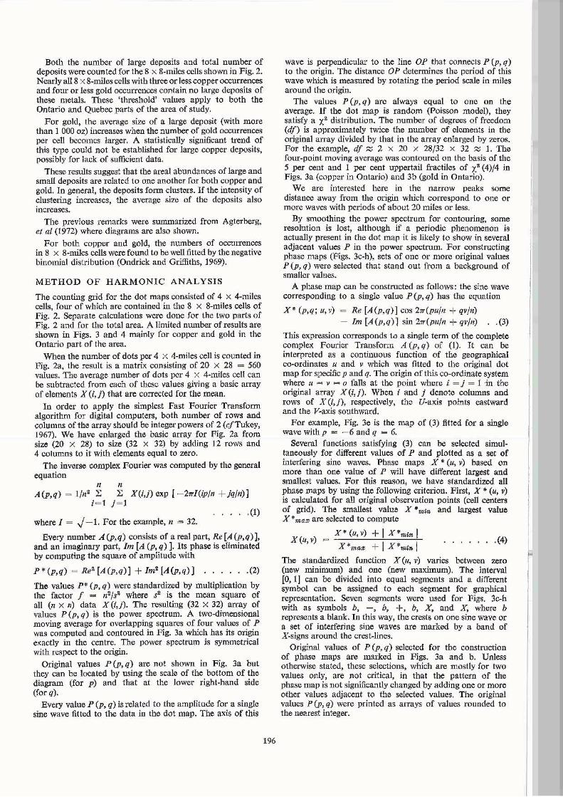
Fig. I. Generalized geological map for part of the Superior Province; based on Geological Map of Canada by R. I. W. Douglas (G.S.C. Map 1250A). Area of study is outlined.

193

The procedure consists of coding dot maps as shown in Fig. 2 and applying a method of harmonic analysis. This method was used to investigate whether there exist zones with alternating high and low densities of occurrences in the areal distribution patterns for copper and gold deposits in the Abitibi area. The statistical method is analogous to the better known methods of optical data processing and X-ray analysis which are based on the diffraction of light (Born and Wolf, 1959). Suppose that a pattern consisting of a set of equally-spaced lines is processed to obtain the diffraction pattern (Pincus and Dobrin, 1966). The result is a single dot in the diffraction pattern at which all the light is concentrated. The location of tillS dot is determined by (i) the direction of the lines in the original pattern and (ii) the perpendicular distance between adjacent lines.

An analogous result can be obtained by coding the pattern and calculating the two-dimensional inverse Fourier transform. This results in the power spectrum which is a numerical analogue of the diffraction pattern. Peaks in the power spectrum may correspond to periodic regularities in the regional arrangement of the dots. These peaks can be evaluated for statistical significance by approximate X2 tests. The emphasis in this paper is on geological application. Several aspects of this method to calculate power spectra have been discussed elsewhere (Agterberg, 1969). The applica­tion described in this paper is comparable with Bartlett's (1964) method for analyzing dot maps.

H is emphasized that the present method was designed to detect pcriodicities in clusters of deposits. If the method is used for other purposes, the results will be only approximate because of distortions related to the boundaries of the area of study. Distortions of this type can be eliminated readily only if the peaks in the power spectrum are narrow and well defined as for periodical regularities.

The areal phenomenon that corresponds to one or more relatively high values forming a peak in the power spectrum can be plotted on the map of the original data (dot map) as contours for one or more interfering waves. For convenience. the resulting contour map is called a phase map, since waves whose amplitudes are represented in the power spectrum are mapped on the basis of their phases also. Phase maps can be evaluated by comparison with the original dot maps and with patterns of known and inferred lineaments in the area or with trajectories constructed by Kutina's method. For evaluation of patterns for interfering waves in a phase map, it can be helpful to trace the crestlines of the maxima which are generally elongated.

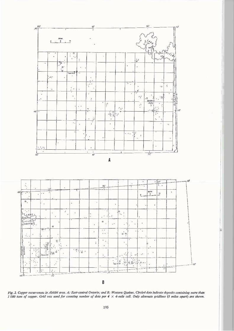
Before discllssing results obtained by this method of harmonic analysis, we first consider the nature of the data on occurrences (see next section). Figure 2 was adapted from a map at scale 1 : 500 000 by Agterberg, et af (1972). In total, 7lS copper occurrences were used for harmonic analysis, and 1257 gold occurrences plotted on another (1 : 500 (00) map in that paper.

SELECTION OF COPPER AND GOLD OCCURRENCES AND PRELIMINARY STATISTICAL ANALYSIS

All data for copper and gold occurrences were compiled from existing sources of information, mainly publications and open files by provincial and federal organizations or agencies. Fairly precise estimates of size and average grade for deposits are available for mines (producers or past-producers) and developed prospects. The size and grade of the majority of occurrences, e.g. those plotted for copper in Fig. 2, are not known prccisely for lack of development.

As a rule, a gold occurrence is defined as such if one or more assay values wcre obtained for it so that the presence

194

of an anomalously high concentration of gold in the host rock (mainly quartz veins with well-defined boundaries) was clearly established. On the other hand, small amounts of high-grade copper mineralization (mainly chalcopyrite in different types of rock) are widespread in the area. The definition of a copper occurrence depends rather strongly upon subjective geological reasoning. The attempt was made to select in a consistent manner mineralized zones with relatively abundant chalco­pyrite in disseminated form and/or in blebs of massive sulphides. These zones were plotted as copper occurrences on the map and many smaller copper showings reported in the literature were not included. For the majority of copper occurrences in Fig. 2, we adopted criteria used by Shklanka (1969) for Ontario and by Dugas, et af (1967) for the Noranda­Val-d'Or area in Quebec. Separate occurrences of copper (or gold) within the same claim C! x t mile) or group of adjacent claims generally are represented as a single occurrence on the map.

Although the study area is exceptionally well explored, the resulting dot maps for copper (Fig. 2) and gold (not shown) are not completely representative of the regional distribution of occurrences for these metals at the surface of bedrock. Glacial debris of various types is abundant in the area forming E-W or ESE-WNW trending belts and N-S or NNW-SSE trending eskers. On the whole, the bedrock is poorly exposed according to irregnlar patterns of outcrops. At one place in the vicinity of Kirkland Lake, glacial cover was 738 ft thick.

An arbitrary network of 4 X 4-miles cells was placed on top of the area. Initially, both occurrences and grid were plotted on geological maps at a scale of one inch to four miles. Alternate grid lines, which are eight miles apart, are shown in Fig. 2.

The numbcr of dots in a cell is determined by one or more of the following factors: (a) abundance of copper deposits at or near the surface of

Archcan bedrock; and (b) abundance and types of outcrops; (c) type and emphasis of exploration activity and amount of

interpretation done by individuals or mining and exploration companies on the basis of local geology and geophysical and/or gcochemical surveys, and

(d) standards set by different exploration geologists for the occurrence of copper or gold,

Our target of study is given by the flrst of these four factors. In practice, it was not possible to consider the other factors in detail and to eliminate their effects, mainly because the abundant information in existence for these factors is widely scattered. Moreover, much information, especially for factors (c) and (d), has been lost or is still kept confidential. The objective of this study was limited to the detection of periodicities in the dot maps. Such phenomena, if present, may reflect certain aspects of the true areal variability of mineralization in bedrock. The other factors, particularly (c) and (d), are more likely to result either in large-scale, systematic trcnds in the patterns, which are artificial, or in more local, irregular distortions.

The quality and quantity of information on mineral deposits increase, as a rule, with the amount of development and/or mining done. Forty-one copper deposits with known total production and/or reserves greater than 1 000 tons of copper are marked by cireles in Fig. 2. This cut-off level for size is arbitrary but data on the selected large deposits w·e based all extensive development.

A similar cut-off level for gold deposits was set at 1 000 oz. of gold. In total, there are 163 gold deposits of this type. The large deposits of both copper and gold were found to have lognonnal distributions.

•

.'W~---------'---------'if '---~-, ---- ~~.

- "

, 0

, "

.'

,-

I , ---jf--o-+--+ -+~+----II~ i

i -+--+-l--j -1---' ,- +---C---l,l I , "

," '.G! . ' 0

.. ;IZ , -.... ;"- ~ \~

~~ -. --I---+-+-t~, +--j~'+-"'~'+--I---+- ' "1"..,..' +----1 ;!~ '~: ;. '.' p

il f-- 1-+--+, ,--j~+--+---

i ~.~'~"~'-============~~~~~,====:==~~"~"~~~"_",,,,,,l -,~,~-L,,_, __ =-.~

A

P"'l1 ;~ . , • , '",:" cr'---+ -t--

! 11

'\ " ,' " 'I' --+-"r- -'---+-- -j- - +-, "

"I ~r I ,;1 I

l~ I-," "

r=i"-";' " ,,,;,c.-, -+-,-, -.J. ,- t-+ -- -j,-t-+--+ . ::. '.';&. <3'i, 1 ·_· ... ··1 : ,

+-- -+--+-f--+.--" -0, .'" ,'" \ '. :' :', . i ... 1 ~'O' • t G. ~.:, .'~ ,c-='ic~---I--!L;lo=" ___ '11"1"

4- ,. L_-'-'r=,="'==2==-='-~-'-~="~"I",,,,,.,-=--C,-,-;_--....L-_'.L __ ~--'-_" -49' ~--' --

B

Flg.2. Copper occurrence,' in Abit/hf area. A: Eas/-central Ontario; and B: W(!Jfern Quebec. Circled dots indicate deposft! containing more than 1 000 Ions of copper. Grid was used for cOIINtlng number of dots per -I x 4-mlfe cell. Only alternate gridfin~s (8 miles apart) are shown.

195

I

r

Both the number of large deposits and total number of deposits were counted for the 8 x 8-miles cells shown in Fig. 2. Nearly all 8 x 8-miles cells with three or less copper occurrences and four or less gold occurrences contain no large deposits of these metals. TIlese 'threshold' values apply to both the Ontario and Quebec parts of the area of study.

For gold, the average size of a large deposit (with more than 1 000 oz) increases when the number of gold occurrences per cell becomes larger. A statistically significant trend of this type could not be established for large copper deposits, possibly for lack of sufficient data.

These results suggest that the areal abundances of large and small deposits are related to one another for both copper and gold. In general, the deposits form clusters. If the intensity of clustering increases, the average size of the deposits also increases.

The previous remarks were summarized from Agterberg, et al (1972) where diagrams are also shown.

For both copper and gold, the numbers of OCCU1TCnccs in 8 x 8-milcs cells were found to be well fitted by the negative binomial distribution (Ondrick and Griffiths, 1969).

METHOD OF HARMONIC ANALYSIS

The counting grid for the dot maps consisted of 4 x 4-miles cells, four of which are contained in the 8 x 8-miles cells of Fig. 2. Separate calculations were done for the two parts of Fig. 2 and for the total area. A limited number of results are shown in Figs. 3 and 4 mainly for coppcr and gold in the Ontario part of the area.

When the number of dots per 4 x 4-miles cell is counted in Fig. 2a, the result is a matrix consisting of 20 x 28 = 560 values. The average number of dots per 4 X 4-miles cell can be subtracted from each of thesc values giving a basic array of elements X (i, j) that are corrected for the mean.

In order to apply the simplest Fast Pourier Transform algorithm for digital computers, both number of rows and columns of the array should be integer powers of 2 (cjTukey, 1967). We have enlarged the basic array for Fig. 2a from size (20 x 28) to size (32 x 32) by adding 12 rows and 4 columns to it with elements equal to zero.

The inverse complex Fourier was computed by the general equation

n A(p,q) = 1/n2 1:

i=1

n :E X(i,j) exp [ -21rI(ip/n + jq/n)]

j=l .••. (1)

where I = .j -1. For the example, n = 32.

Every number A (p,q) consists of a real part, Re [A (p,q) ], and an imaginary part, Im [A (p, q) ]. Its phase is eliminated by computing the square of amplitude with

P'(p,q) = Re 2 [A(p,q)] + Im2IA(p,q)] ••.••. (2)

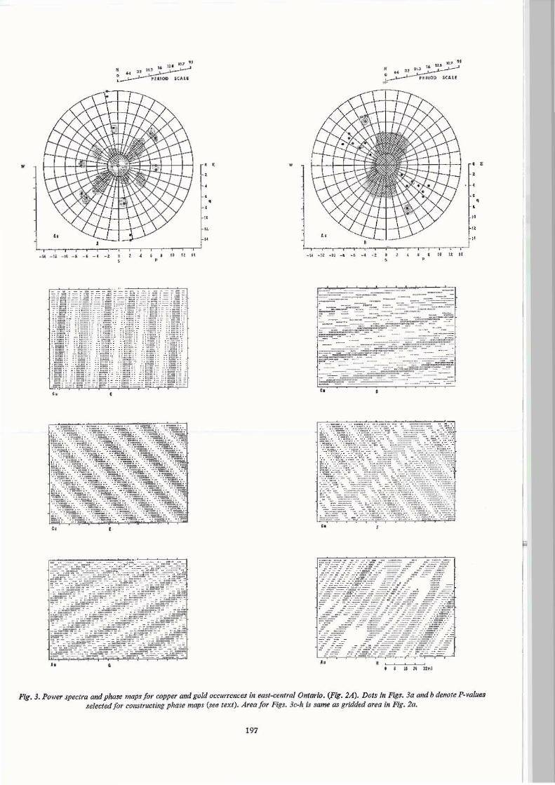
The values P' (p, q) were standardized by multiplication by the factor j ... n2/s~ where $2 is the mean square of all (n x n) data X(i,j). The resulting (32 x 32) array of values P (p, q) is the power spectrum. A two-dimensional moving average for overlapping squares of four values of P was computed and contoured in Fig. 3a which has its origin exactly in the centre. The power spectrum is symmetrical with respect to the origin.

Original values P (p, q) are not shown in Pig. 3a but they can be located by using the seale of the bottom of the diagram (for p) and that at the lower right-hand side (for q).

Every value P (p, q) is related to the amplitude for a single sine wave fitted to the data in the dot map. The axis of this

196

wave is perpendicular to the line OP that connects P (p, q) to the origin. The distance GP determines the period of this wave which is measured by rotating the period scale in miles around the origin.

The values P(p,q) arc always equal to onc on the average. If the dot map is random (Poisson model), they satisfy a Xl distribution. The number of degrees of freedom (d!) is approximately twice the number of elements in the original array divided by that in the array enlarged by zeros. For the example, dj ~ 2 x 20 x 28/32 x 32 ~ 1. The four-point moving average was contoured on the basis of the 5 per cent and 1 per cent uppertail fractilcs of Xl (4)/4 in Figs. 3a (copper in Ontario) and 3b (gold in Ontario).

We are interested here in the narrow peaks some distance away from the origin which correspond to one or more waves with periods of about 20 miles or less.

By smoothing the power spectrum for contouring, some resolution is lost, although if a periodic phenomenon is actually present in the dot map it is likely to show in several adjacent values P in the power spectrum. For constructing phase maps (Figs. 3c-h), sets of one or more original values P (p, q) were selected that stand out from a background of smaller values.

A phase map can be constructed as follows: the sine wave corresponding to a single value P(p,q) has the equation

X* (p,q; u, v) = Re [A(p,q)] cos 21r(pu/n + qv/n) - Im [A(p,q)l sin 21r(pu/n + qv/n) .. (3)

This expression corresponds 1a a single term of the complete complex Pouricr Transform A (p, q) of (1). It can be interpreted as a continuous function of the geographical co"ordinates u and v which was fitted to the original dot map for specific p and q. The origin of this co-ordinate system where u - v - 0 falls at the point where i = j = 1 in the original array X (i, j). When i and j denote columns and rows of X(l,j), respectively, thc U-axis points eastward and the V·axis southward.

Par example, Fig. 3e is the map of (3) fitted for a single wave with p = -6 and q - 6.

Several functions satisfying (3) can be selected simul­taneously for different values of P and plotted as a set of interfering sine waves. Phase maps X * (u, v) based on more than one value of P will have different largest and smallest valucs. For this reason, we have standardized all phase maps by using the following criterion. First, X'" (u, v) is calculated for all original observation points (cell centers of grid). The smallest value X'" mln and largest value X' maz are selected to compute

X() X' (u, v) + I X'mln I

u,V = X'ma:!: + I X'mjJ$1

...•... (4)

The standardized function X(u, v) varies between zero (new minimum) and one (new maximum). The interval [0,1] can be divided into equal segments and a different symbol can be assigned to each segment for graphical representation. Seven segments were used for Pigs. 3c-h with as symbols b, -, h, +, b, X, and X, where b represcnts a blank. In this way, the crests on one sine wave or a set of interfering sine waves are marked by a band of X-signs around the crest-lines.

Original values of P (p, q) selected for the construction of phase maps arc marked in Pigs. 3a and b. Unless otherwise stated, these selections, which are mostly for two values only, are not critical, in that the pattern of the phase map is not significantly changed by adding one or more other values adjacent to the selected values. The original values P (p, q) were printed as arrays of values rounded to the nearest integer.

•

_" . '1 _" • • . , ., -.

"

.. ,,. .. , ., "~."l . " H~'OO I ~"'"

, • " .t " •

, •

..

.. ,,. "" .. .~.,O . .. ~ ... ' O~ .CA Lf

........... _. " .... :=::-~/:: :: ... . "''''" ...

,-• ..

" ,

,

Fig. 3. Power spel!tra mu! phase maps for copper and gold occurrenc~s in east-central Ontario. (Fig. 2A). Dots In Figs. 3a and b denote P-values selel!ted for constructing phase maps (see text). Area for Figs. 3c-h is sam~ as gridded area in Fig. 20.

197

Phase maps fur copper and gold occurrenCt!s In east-cenlral Ontario

Copper N·S set: P(7,O) ~ 4 and P(7,l) = 5

These two values also appear as a small peak in Fig. 3a. The corresponding waves are approximately in phase and combined give Fig. 3c. The crest-lines form a N-S set and are about 20 miles apart.

Copper E-W &et: P(t,G) = 4 and P(1,7) = 5; P(2, 13) = 3 a nd P('2, 14) = 5

T bis combination of four waves (Fig. 3d) corresponds to two peaks in the unsmootbed power spectrum. In Fig. 3a, only the fint peak can be seen. The second is. a harmonic o f the first one. The four waves are approximately in pbase. Tbose for the second peak have tile effect of flattening the maxima and minima of the waves for the first peak.

Copper SE-NW set (1): P( - 6, 6) "" 7

This phase map (Fig. 3e) is for one wave only. It can also be seen in Fig. 3a. The largest P-value adjacent to P (-G, 6) was added to give:

Copper SE-NW set (2): P( - 6,G} ... 7 and P( -7,5) = 4

Thcsc two waves (Fig. 3f ) arc 1101 in phase. The S&NW set canllot be defined as clearly as the previous sets. Tbe difficulty may be caused by the fact that this peak. in part, could be a harmonic of the rather prominent peak for the same direction but closer to the origin in Fig. 3a.

1f crest lincs are constructed through the zones of X-signs in Figs. 3e, d, and e, the result is three sets of lines which aTe approximately equidistant and straight. The three sets intersect at approximately the same points which suggests that tlley are mutually interrelated, This regular pattern is somewhat distorted if P ( - 7,5) is also considered .

The gold spectrum (Fig. 3c) differs significanUy from the copper sptttrum (Fig. la). The following two phase maps for gold occurren~ are shown in F igs. 3g and h.

Gold WSW-ENEset: P (4, 8) "" 7 and P(4,9) = 4

This pair ofP-values stands out clearly from the background. The two wave9 are approximately in phase (Fig. 3g).

Gold SW-NE set: P(3,2) .,. 4: P(4,4) .., 4; P(5, 3) - 3; P(6,4) - 3;P(7,S) - 2;P(7,6) - 5; P(8,4) - 2.

This phase map (Fig. 3h) is not based on a single peak but on seven relatively 1!lCgC P-values whicb form a n ill~fioed ridge ill the origioal power spectrum. Only part of this ridge is shown in the contoured patlern o f rig. 3b. It can be regarded as a rather strongly distorted SW.NE-trendina: set of waves with period of about 15 miles. The crest lines of this set hove a distinct tendency to pass through the intersection points of the three sets for copper.

The spectra shown in Figs. 3a and b were tested for consistency by varying the size of array and using a diffcrent grid (or coding. In addition to th!! enlarged array of size (32 X 32), we also used a (64 X 64) array by inserting 3 072 more :reros. This gave similar results.

We used the U niversal Transverse McrcalOr grid for coding with spacing of 10 km instead of four miles. The ceUs for this other grid arc 2.41 times larger in area. The throosots for copper now could be rcrosnized when the (64 x 64) enlarged array was used. The peak for the E-W set becomes better pronounced when cell sizc is enlarged but those for the N-S and SE-NW sets decrease in magnit ude.

The patterns derived for the Ontario part of the Abitibi belt caonot be recognized in spectra for the Quebec part

198

(Pig. '2b) where most powt'r is concentrated near the origin for both copper and gold occurrences.

Analysis of photographic negatives of the dot maps at the Kansas Geological Survey, Lawrence, Kansas, gave diffraction patterns similar to the power spectra. More harmonics were developed in the diffraction pauems. A detailed comparison of results for thc two methods wns not made.

nle two parts of the area were combined and run by using a (64 x 64) enlarged array. No periodical phenomena wilh spacing of '20 miles or less WCJe evident from these runs. Crest lines for a phase map (or copper occurrences in total area are SbOWD io F ig. 5. T hey come from a phase map based on P (4. 0), P (-4, 1), P ( - 4, 2) and P (3, I) which form 11. d islinct peak: in the spectrum.

GEOLOGICAL INTERPRETATION AND SlGN IFICANCE FO R EXPLORATlON STRATEGY

A detailed comparison of Figs. 3c-f with Fig. 2a indicates that the dots tend to cluster in many places around the crest lines. It should be kept in mind that the periodical features are weaker than the main systematic al'ca1 variations in density which correspond to P-values closer to the origin of the power spectrum. Some crest lines and parts of others in Figs. 3c-f are no t associated with a significant number of copper occurrences, especially iD plllces. where they cross gmnitic intrusions or areas covered by a relatively thick layer of glacial debris.

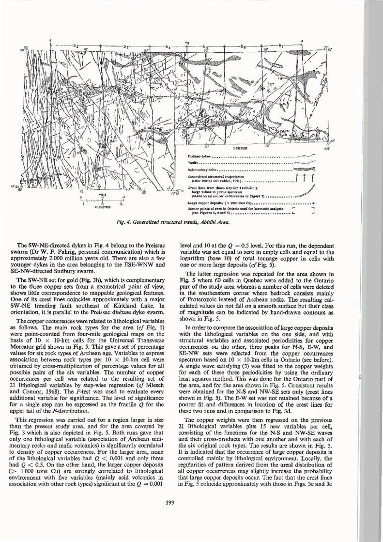
A comparison of the phas!! nmps with geological features in the area indicates that the sets of crest lines are closely related to tectonic lineaments in a number of places. Major faults, diabase dykes and Archean sedimentary belts for the area are shown in Fig. 4. For the western part of the area, these fea tures were adopted from the 16-mile geological map (No. 2198) published by the Ontario Department of Mines a nd Northern Affail'3 iD 1971. For Utc other pan of thc area, a vsricty of geological maps wag consulted.

AJso shown in Fig. 4 is a N-S set of stmcturai trajectories inferred by Kutina and Pabbri (1971) for the Abitibi Belt (see Introduction). The three trajectories falling in Ontario correspond rather closely to alternate crest lines in Fig. 3e for too copper N-S set.

The SE-NW set for copper is related to known faults in seve~al places. Crest lines of Fig. 3e (and f) coincide approximately with (i) the Moutreal River Fault that extends soutlteastward from Timmins; and (ii) the major SE-NW fault crossing Lake Abitibi.

The previous correlations are only approximate since there are Slight departures in direction between faults and crest lines.

A structural correlation for the copper B-W set is less clear. The crest lines for this set (Fig. 3d) have a distinct tendency to coincide with the occurrences of Arehean sedimentary beJts in OntaJio. The latter occur either at the centers of approximately B-W trending synelincs or in grabens bounded by fau lts or shear zones.

Tlte three sets fo r copper are related to the three main structural trends in the area. The N-S trend is accompanied by many diabase dykes of the N-s-directed Matachewan swarm dated at approximateJy 2485 million years old (Fahrig, et aI, 1%5). T he other main swann of diabasc dykes ill the area (Abitibi swarm) trends WSW-ENE and is approximately 1 230 million yean old (Fahrig, et ai, 1965). It cuts the Proterozoic sediments of the Cobalt group in the southeastern part of the study area in Ontario (sce Fig. 1). T he WSW-ENE set for gold (Fig. 3g) is parallel to this younger trend.

• , , •

LlOEIID

Dl>.bt. .. <I1l<-............... . ................ ....... " ...... ___ ____

eM............, ........ .... .......... ........................... =::aa'll!l

.-...,1I...t ... ,... .... ,,~ " -1 ,,!lo. __ ~I, 1" 1) .. ........... .. , .... .......... .

C"...ll hIQ fr .... "" . ... .. Ol''''''' ........ ivolj' ../ ktif' •• 1 ." ,~ """"" lI>OOlr_ (bt.oo4 .. aU _ ___ of 1'1,.... *} •••••• " •••••••• •

........ _ ........ tI( ) l _ _ DI) • •••••• •• • ••• • • ••• ••••• •• • •• •• • • •••

CHt><-. IIOI ... oI.r • • ". _ _ f<>< -.-. _lpI r -, { ... 1'I(V'H2.laO<!4) ....................... "........... .J

Fig. 4. Generalized structural tnnds, Abitibi Arl.'a.

The SW-NE-directed dykes in Fig. 4 belong to the Preissac swarm (Or W. F. Fahrig.. personal communication) which is approximately 2000 million years old , There arc: also a few younger dykes in lbe area belonging to tbe ESE-WNW and SE-NW-directed Sudbury swarm.

The SW-NE set for gold (Fig. 3h), which is complementary to the three copper sets from a geometrical point of view, shows little correspondence to mappable geological features. One of its crest lines coincides approx.imately with a major SW·NE trending fault $Cutheast of Kirkland Lake. In orientation, it is parallel to the Preissac diabase dyke swarm.

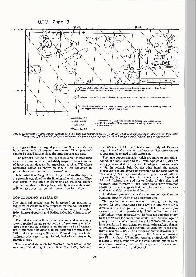
The copper occurrences were related to lithologlcaJ variables as foDOM. The main rock types for the area (cl Fig. J) were point-counted from four-mile geological maps on the basis of 10 x l()"'km cells for the Universal Transverse Mercator grid shown in Fig. 5. This gave a set of percentage vaJues for six. rock types of Archean age. Variables to express association between rock types per 10 X Io...km cell were obtained by closs-multiplication of percentage values for all possible pairs of the six variables. The number of copper occurrences per cell was related to the resulting set of 21 Iithologica] variables by step.-wise regression (c! Miesch aDd Connor, 1968). Th6 F·test wu used to evaluate every additional variable for significance. The level of signi6cance for a single step can be expressed as the fractile Q for the upper tail of the P-distribution.

This regression was carried out for a region larger in size than the present study area, and for the area covered by Fig. 3 which is also depicted in Fig. 5. Both runs gave that only one lithological variable (association of Archean sedi­montary rocks Illld mafic volcanics) is slgnificantly correlated to density of copper occurrences. For the larger area, none of the lilbological varia bles had Q < 0.001 and only three bad Q < 0.5. On the other hand, the larger copper deposits (> I 000 tons Cu) are strongly correlated to lithological environment with five variables (mainly acid volcanics in association with other rocJc types) significant at the Q - 0.001

199

level and 10 at the Q = 0.5 leveL For this run, the dependent variable was set equal to zero in empty cells and equal to the logarithm (base 10) of total loconae copper in cells with one or more large deposits (c/Fig. 5).

The latter regression was repeated for the area shown in Fig. 5 where 60 celb in Quebec were added to the Ontario part of the study area wherea8 a number of cells were deleted in the southeastern corner wbe~ bedrock consists mainly of Proterozoic instead of Archean rocks. The resultina: cal­culated values do not fall on a Amooth surface but their cta" of maa:nitude can be indicated by hand-drawn contours as shown in Fig. 5.

In order to compare the association of large copper depoaitll with the lithoiogical variable!! on the one side, and with structural variables and associated periodicities for copper occurreuCCll on the other, three peaks for N-S, E-W, and SE-NW sets were selected from the copper occurreoces spectrum based on 10 x to-km cells in Ontario (see before). A single wave satisfying (3) was fitted to tile copper weights for each of these three periodicities by using the ordinary least squares method. This was done for the Ontario part of tbe area, and for the area. shown in Fig. 5. Consistent results were obtained for tbe N-S and NW-SE sets only (crest lines shnwn in Pig. 5). TIle Eo W sel was not retained because of a ponrer lit and differeoces in location of the crest lines (or these two runs and in comparison to Fig. 3d.

The copper weights were then regressed on the previous 21 litbological variables plus 15 new variables per cell, consistiug of the functions for the N-g and NW-SE wave;, and their cross-products with one another and with each of the six original rock types. The results are shown in Fig. 5. It is indicated that the occurrence of large copper deposits is controlled mainly by Jithological environment. LocaJly, the regularities of pattern derived from the areal distribution of all copper occurrences may slightly increase the probability that large copper deposits occur. The fact that the crest lines in Fig. 5 coincide approximately with those in Figs. 3c and le

U.TM. Zone 17 SOO'ME

, .. .. "

S"I. " " .. •• O C,lIlier of 10 x 10 km. UTM oell with OWl or more oopper dopo. [I. (I',,"," thon 1000 10;0.' C~ por

5 d~.!!). Wolght i . log.\dlhrn (\>o.. e 10) of total loan"le cower por coH, .

g;6 s<ro.matio eonlour. 10< va lue. obt~inO" by rc~<.uioo of o""l"'r we l&l!ls on Zl mholO\ric ol variable ••

_ie •• th.n.-O.5 __ 0.510_Q.25

+ O.2~toO.S

+ "'<><'0 than 0.5

}

Diffor"""". tor Ul'loI coU. botwe .... (1) Ilcgl'en ion 01 c_ ",. ight. on ~llilhol~loa1"'d 1~ ba<moni. variable_; ... <1 (2) ditto OIl 21 litho-­log;" . l .. riabIe • •

Fig. S. Occurrence of large copper deposits (> 1 000 tons Gu) quantified for 10 x 10 km UTM cells and r~lated to lithology for these celll. Comparison ofTithological arid structural control for large copper deposits (bused on harmonic analysis for all copper occurrences).

also suggests that the large deposits have these periodicities in common with all copper occurrences, This hypothesis cannot be tested further since the large deposits are rare.

The previous method of multiple regression has heen used as a first step to construct probability maps for the occurrence of large copper deposits by Agterberg, et aI, (1971) where calculated values as shown in Fig. 5 are converted to probabilities and interpreted in more detail.

It is noted that for gold both larger and smaller deposits are strongly correlated to the lithological environment. They may occur in the same environments as the large copper deposits but also in other places, notably in association with sedimentary rocks that contain layered iron formations.

CONCLUDING REMARKS

The statistical results can be interpreted in relation to sequences of events in time proposed for the Abitibi Belt in recent models of its metallogenic evolution (see Douglas, 1970, Editor; Goodwin and Ridler, 1970; Hutchinson, et aI, 1971).

The oldest rocks in the area are volcanic and sedimentary rocks deposited in an eugeosyncline of Archean age. Most large copper and gold depostis are thought to be of Archean age, Many would be older than the Kenoran orogeny (about 2480 million years ago; Stockwell 1964) during which the Archean rocks were strongly folded, faulted and intruded by granitic stocks,

The dominant direction for structural deformation in the area was N-S during Archean time. The E-W. N-S and

200

SE-NW-directed folds and faults are mainly of Kenoran origin. Some faults were active afterwards, The three sets for copper may be related to this toctonism.

The large copper deposits, which are more or less strata­bound, and most large and small vein-type gold deposits are strongly correlated to specific lithological environments within the volcanic belt. On the other hand, the smaller copper deposits are almost uncorrelated to the rock types in their vicinity, hut they show distinct regularities of pattern. Regionally, they are related to the occurrence of synclinal folds of Archean age and major faults of that time and younger. Locally, many of them occur along shear zones not shown in Fig. 5, It suggests that their place of occurrence was controlled mainly by structural factors.

All diabase dyke swarms in the area are younger than the Kenoran orogeny which closed Archean time.

The only harmonic components in the areal distribution pattern for gold occurrences have SW-NE and WSW-ENE directions, The two gold sets are parallel to diabase dyke swarms dated at approximately 2000 million years and 1 230 million years, respectively. Thefirst set is complementary to the three sets for copper and could be of Archean age or younger. On the other hand. the gold WSW-ENE set may have been formed later. during Proterozoic time, after a change in dominant direction for structural deformation in the area from N-S to NNW-SSE. Thelatterdirection was also dominant during the Grenvillian orogeny in the Grenville Province (see Fig. 1), about 955 million years ago (Stockwell, 1964). It suggests that a minority of the gold~bearing quartz veins was formed relatively late in the sequence of events and subject to regional structural control.

ACKNOWLEDGEMENTS

Thanks are due to Dr J. S. Springer for assistance in the compilation of a data file for copper and gold occurrences in the Abitibi area, and to Mr C. F. Chung for preparation of FORTRAN computer programs and construction of Fig. 3.

Contribution of data from open me by the following organizations is gratefully acknowledged: Mineral Resources Branch, Department of Energy Mines and Resources, Ottawa; Ontario Department of Mines and Northern Affairs, Toronto; Quebec Department of Natural Resources, Quebec.

REFERENCES

AGTERBERG, F. P. (1969). Inte~polation of areally distributed data. Colo. Sell. Mines Q. vol. 64, pp. 217-237. AGTERBERG, F. P., CHuNG, C. F., FABBRl, A. G., KELLY, A. M., and SPRINGER, J. S. (1972). Geomathematical evaluation of copper and zinc potential of the Abitibi area, Ontario and Quebec. Geol. Surv. Can. Paper 71-41 (in press). BARTI.E1T, M. S. (1964). The spectral analysis of two-dimensional point processes. Biometrika. vol. 51, pp. 299-311.

BORN, M., and WOLF, E. (1959). Principles 0/ optics. pp. 369-457. Pergamon Press, New York. DoUGLAS, R. J. W., Editor (1970). Geology and economic minerals of Canada. pp. 43-226. Geol. SUry. Can., Econ. Geo!. Report No. 1, Ottawa. DUGAS, J., LATULU'l'E, M., and DUQUETIE, G. (1967). Annotated bibliography on the metallic mineralization in the regions of

201

Noranda, Matagami, Val-d'Or, and Chibougamau. Dept. Nat. Res. Quebec, Special Report no. 2. FAHRIO, W. F., GAUCHER, E. H., and LAROCHELLE, A. (1965). Palaeomagnetism of diabase dykes of the Canadian Shield. Call. J. Earth Sel. vol. 2, pp. 278-298. GOODWIN, A. M., and RrDlllR, R. H. (1970). The Abitibi Orogenic Belt. Geol. Surv. Can. Paper 70-40, pp. 1-30. HurCHINSON, R. W., RIDLER, R. H., and SUFFEL, G. G. (1971). Metallogenic relationships in the Abitibi Belt, Canada: A model for Archean Metallogeny. Can. Min. Metal!. Bull. vol. 64, no. 708, pp. 48-57. KUTINA, J., and FABBRI, A. G. (1971). Relationship of structural lineaments and mineral occurrences in the Abitibi area of the Canadian Shield. Geol. Surv. Can. Paper (in press). MIESCH, A. T., and CONNOR, J. J. (1968). Stepwise regression and nonpolynomial models in trend analysis. Kansas Geol. Surv. Computer Contr. no. 27. ONDRICK, C. W., and GRIFFlTHS, J. C. (1969). Fortran IV Computer Program for fitting observed count data to discrete distribution models of binomial, Poisson and negative binomial. Kansas Geol. Surv. Computer Contr. no. 35. PlNc(Js, H. J., and DOBRIN, M. B. (1966). Geological applications of optical data processing. J. Geopllys. Res. vol. 71, pp. 4861-4869. STOCKWBLL, C. H. (1964). Fourth Report on structural provinces, orogcnics and time-classification of rocks of the Canadian Precambrian Shield. Geol. Surv. Can. Paper 64-17. SHKLANKA, R., Editor (1969). Copper, nickel, lead and zinc deposits of Ontario. Ontario Dept. Mines, Mise. Paper, no. 37. TUKEY, J. W. (1967). An introduction to the calculations of numerical spectrum analysis. pp. 25-46. Spectral analysis 0/ time series, B. Harris, Bd. Wiley, New York.

I I

I

202

I

r