harvard catalyst journal club. understanding the ... the method for selecting doses further from the...

1

Harvard Catalyst Journal Club: “Performance of toxicity probability interval based designs in contrast to

the continual reassessment method “

Horton, Wages and Conaway, Statistics in Medicine, 2017

Edie Weller, Ph.D.

Director, Biostatistics and Research Design Core of the Institutional Centers for Clinical and

Translational Research at Boston Children’s Hospital

August 29, 2017

Other papers…

• CRM

– O’Quigley, Shen (Biometrics 1996, ref 1)

– O’Quigley, Pepe, Fisher (Biometrics 1990,ref 16)

– O’Quigley, Iasonos (Statistics in Biopharmaceutical Research 2014, ref 8)

– Wages, Conaway and O’Quigley (Clinical Trials 2013)

– Iasonos, O’Quigley (Journal of Clinical Oncology 2014, ref 11) review of model

guided phase I clinical trials

– Many others….

2

Other papers…

• mTPI

– Ji , Liu, Li, Bekele (Clinical Trials 2010, ref 12)

– Ji Y, Wang SJ. (Journal of Clinical Oncology 2013)

– Guo W, Wang SJ, Yang S, Lynn H, Ji Y (Contemp Clinical Trials 2017,

mTPI2)

• BOIN design

– Liu and Yuan (Applied Statistics 2015, ref 13)

– Yuan, Hess, Hilsenbeck, and Gilbert (Clinical Cancer Research 2017)

– Lin and Yin (Stats methods research 2015, combination trials)

3

Background

Phase I oncology trials:

• Most common is 3+3 design

– Easy to implement but less efficient than model based methods

• Continual reassessment method (CRM)

– Most widely recognized model based method

– Challenge to implement but more efficient

• Two potential alternatives

– Modified toxicity probability interval (mTPI)

– Bayesian optimal interval (BOIN)

• Horton et. al paper evaluates these alternatives relative to CRM by simulation

4

Background: Pediatric Oncology Phase I Trials

90 studies published between 2009-2014

Doussau et al. (2016) Contemp Clin Trials. 47: 217–227.

Nu

mb

er

of

stu

die

s

5

Notation:

DLT = Dose limiting toxicity

θ = Target probability of toxicity

K = Number of available dose levels

dk = Dose at level k

πk = Probability of DLT at dose level k

nk = Number of subjects at dose level k

yk = Number of subjects who experienced DLT(s) at dose level k

6

3+3 Design

7

Additional subjects often treated at MTD (expansion cohort) to improve precision

3+3 Design and Variations

• Uses pre-defined set of rules to assign next subject’s dose level

• Advantages:

– Easy to implement and understand

– Conservative in terms of safety

• Disadvantages

– Slow dose escalation

– Many subjects may be treated at sub-therapeutic doses

– “Memoryless”: uses information from most recent dose to determine next

dose; ignores other observed dose information

Le Tourneau, Lee, & Siu. JNCI. 2009; 101(10):708-720

8

CRM Design

• Continual Reassessment Method (CRM):

– Assume an a priori dose-toxicity curve

(e.g. logistic model, power model)

– Select a target toxicity rate (e.g. 30%)

– Update dose-toxicity curve after each

subject’s outcome is observed

– Model recommends optimal dose for

next subject

– End trial using stopping rule: (e.g.

enrolled pre-specified maximum N)

• Many variations exist: modified CRM, time-

to-event (TiTE) CRM, etc.O’Quigley, Pepe, & Fisher. Biometrics. 1990; 46(1):33-48Garrett-Mayer. Understanding the CRM. 2005

Example Dose-Toxicity Curves

Θ=Target DLT rate

9

CRM and Simulation Assumptions:

• Used 2-stage likelihood version of CRM (O’Quigley, Shen 1996)

• Power model used for probability of toxicity at dose dk

ψ(dk,a)=pkexp(a)

– a is scalar parameter

– pi are pre-specified constants (skeleton values), 0<p1<p2<…< pk<1

– Spacing between the skeleton values is important

– Used Lee and Cheung method to obtain skeleton spacing

10

CRM and Simulation Assumptions:

• Approach to ensure heterogeneity in DLT responses:

– 1st stage: single subject cohorts assigned escalating doses until one DLT

and one non-DLT observed

– 2nd stage: ML is used to estimate power model scalar parameter

• Allowed for early termination if the 90% lower confidence limit for the 1st dose

level is greater than target toxicity (θ).

• Used following functions in R package dfcrm :

– CRMOUT function (“MLE” method, “empiric” model)

– getprior function for skeleton (half width= 0.06 , MTD prior guess=dose 2)

11

mTPI and Simulation Assumptions:

• Combines simplicity of 3+3 method and allows for specification of target toxicity probability

• Extension of toxicity probability interval method

• Employs simple beta-binomial model

• Partition interval (0,1) into 3 sub-intervals based on pre-specified constants ε1 and ε2. Default values are ε1= ε2= 0.05.

[0, θ- ε1) => Dose de-escalation

[θ- ε1, θ- ε2) => Dose remains the same

[θ- ε2, 1) => Dose escalation

12

YI and Wang, JCO, 2013, 21(14); 1785-91

mTPI and Simulation Assumptions:

• Calculate the unit probability mass (UPM) for each sub-interval

– Assumes toxicity probabilities (πk ) have independent beta distributions with shape parameters (αk , βk ) and (αk= α+yk and βk= β+nk-yk).

• Interval with highest UPM dictates the decision for the next patient

• Trial is terminated when pre-specified sample size is reached.

• Safety rules incorporated:

– Prevent escalation to a dose that has previously deemed too toxic

– Allow for trial termination if lowest dose too toxic

• Used mTPI webtool found at http://www.compgenomie.org/NGDF/

• Used default values of ε1= ε2= 0.05.

13

YI and Wang, JCO, 2013, 21(14); 1785-91

http://www.compgenomie.org/NGDF/

BOIN Design:

• Optimization is anchored to 3 point (or local) hypotheses.

• Interval boundaries selected to minimize decision error rates

• Define key parameters:

– Max N

– Target toxicity (θ)

– Pre-specified toxicity tolerance interval (default is [0.6θ, 1.4θ])

– Number pts per dose level (nk)

– Probability the dose is less than, equal to, or higher than MTD

(e.g. non-informative prior = 33% for each group)

• With non-informative prior the boundaries are independent of dk and nk

Liu & Yuan. (2015) JRSSC. 64(3): 507-523

14

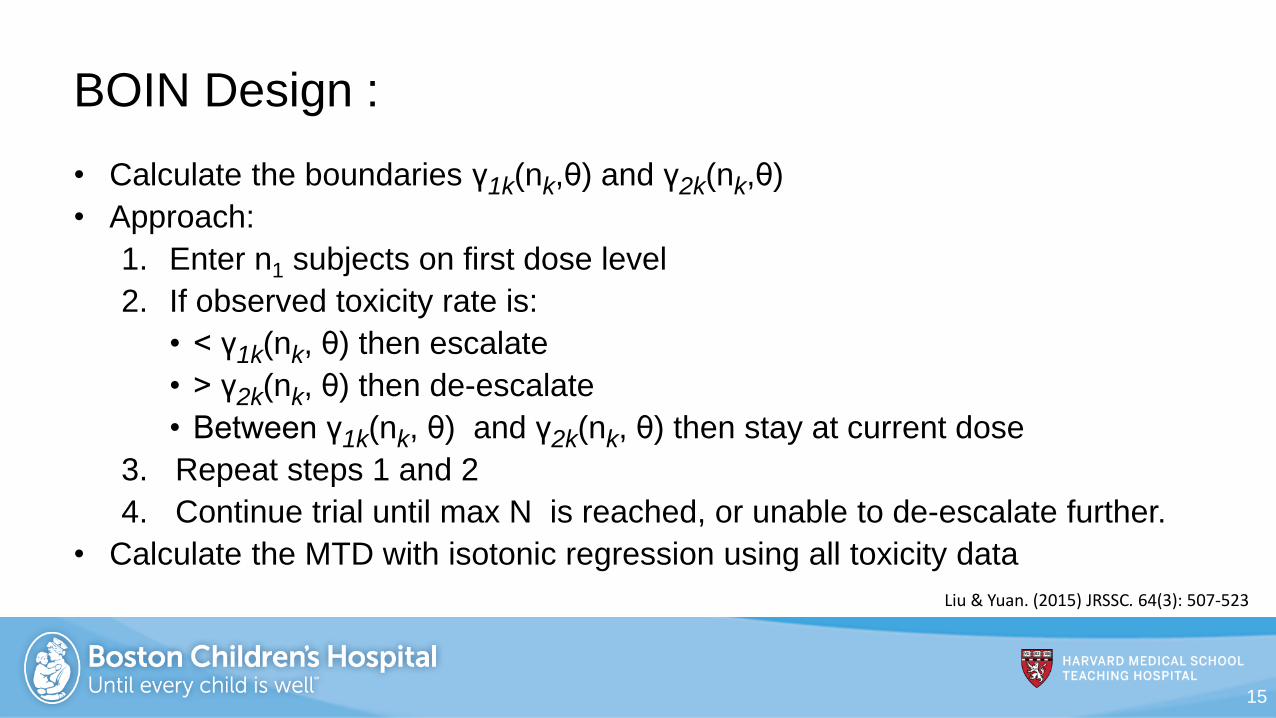
BOIN Design :

• Calculate the boundaries γ1k(nk,θ) and γ2k(nk,θ)

• Approach:

1. Enter n1 subjects on first dose level

2. If observed toxicity rate is:

• < γ1k(nk, θ) then escalate

• > γ2k(nk, θ) then de-escalate

• Between γ1k(nk, θ) and γ2k(nk, θ) then stay at current dose

3. Repeat steps 1 and 2

4. Continue trial until max N is reached, or unable to de-escalate further.

• Calculate the MTD with isotonic regression using all toxicity data

Liu & Yuan. (2015) JRSSC. 64(3): 507-523

15

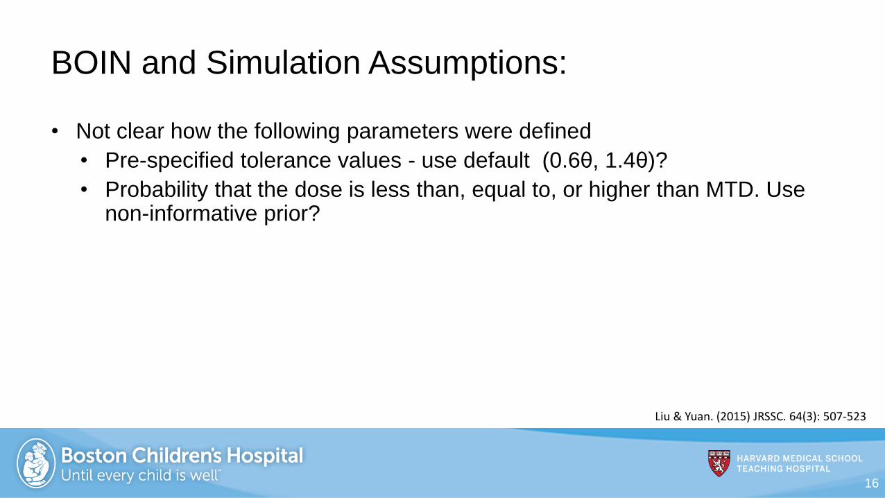
BOIN and Simulation Assumptions:

• Not clear how the following parameters were defined

• Pre-specified tolerance values - use default (0.6θ, 1.4θ)?

• Probability that the dose is less than, equal to, or higher than MTD. Use non-informative prior?

Liu & Yuan. (2015) JRSSC. 64(3): 507-523

16

BOIN vs. 3+3 Design

17

Figure 2: A hypothetical phase I clinical trial using the BOIN design. The numbers indicate the patients identification. Three patients in each box from a cohort.

Yuan, Hess, Hilsenbeck, and Gilbert , Clin Cancer Res; 22(17) 4291-301

Simulation Performance Measures

Measure Definition

Termination Proportion of simulations which terminated early

MTD Selection Proportion of simulations selecting the true MTD

Accuracy index for dose

selection

Incorporates information at all doses levels into 1 number; Penalizes

the method for selecting doses further from the true MTD

Accuracy index for subject

allocation

Same as above but substitute proportion of subjects allocated to dose

k for the probability

Percent correct selection

(PCS)

Probability of selecting true MTD (proportion of simulations select the

dose that minimizes |πk – θ|)

Percent acceptable

selection

Same PCS but considers those doses with πk within 5% of the target

probability toxicity.

18

Simulation Parameters

• θ =0.20

• Number of simulations=2000

• Designs: 4, 6, 8 dose levels

• N=24,36,48 for 4,6,8 dose levels

• 16 dose toxicity curves/design

– 12 with MTD at lower doses

– 4 with MTD at higher doses

• Scenario numbers do not align

across the designs

19

Figure 1. Dose toxicity curves

Horton, Wages and Conaway, Stat in Medicine 2017, 36, 291-300

20


• Proportion higher for BOIN and mTPI as compared to CRM for 4 dose levels (S9, S12), 6 dose levels (S1 ), 8 dose levels (S1) [boxes above]

• In all other scenarios (MTD is not higher than target toxicity) BOIN proportion is a) lower as compared to mTPI , b) within 0.05 of CRM in 45/48 scenarios except 4 dose level (S4,S6) and 6 dose level (S4) [circled above]

21


• BOIN proportion>= mTPI proportion in all designs and scenarios • BOIN proportion within 5 % of CRM in 23/48 scenarios (9/16 4 dose scenarios; 10/16 6

dose scenarios; and 4/16 8 dose scenarios )

22


Figure 2. Accuracy index for dose selection

Note: y-axis ranges differ

Question: how is y-axis calculated?

Authors comments: at 8 dose levels ranking of methods with CRM > BOIN>mTPI

23


Figure 3. Accuracy index for subject allocation

Note: y-axis ranges differ slightly

Authors comments: Similar performance for methods; as increase dose levels ranking of methods with CRM > BOIN>mTPI

24


Figure 4. Percent correct selection


Authors comments: results similar to accuracy; PCS very similar for BOIN and mTPI but with 8 doses BOIN outperforms mTPI.

25


Figure 5. Percent acceptable within 5%


Authors comments: results similar to accuracy and PCS.

Questions:

• Accuracy index is calculated with results from simulations that make a dose

recommendation (page 294)

– Does this imply that the studies who terminate early are not included?

– In table II is the denominator number of simulations or number of simulations that made a

dose recommendation?

– PCS include all simulations in denominator?

26

CRM mTPI BOIN CRM mTPI BOIN

D4S9 0.5 0.26 0.3 0.74 0.76 0.77

D4S12 0.34 0.19 0.24 0.78 0.84 0.82

D6S1 0.43 0.22 0.24 0.74 0.79 0.8

D6S1 0.76 0.53 0.58 0.8 0.71 0.72

Questions:

• For the Scenario 9 (S9) and S12 4 dose designs &S1 6 and 8 dose designs:

– Terminating early is the correct thing to do and have correctly not identified the MTD

– So, should all of the simulations be included when compute the proportion of simulations

recommending the true MTD (Table II)?

– Here termination counts as identifying the true MTD. If so, then the results would be as

follows in green.

27

Questions:

• For all other designs except S9 and S12 4 dose designs and S1 6 and 8

dose designs-

– Terminating early is the incorrect thing to do and therefore, have not found the MTD when

should have.

– Therefore, should all of the simulations be included when compute the proportion of

simulations recommending the true MTD for these designs (Table II)?

28

Questions:

• How do these results compare to the paper by Liu and Yuan?

• This paper compared CRM, mTPI and BOIN approaches

• Simulation parameters:

– 6 dose levels

– Maximum sample size of 36 patients in 12 cohorts of size 3

– Target toxicity θ=0.25

– Tolerance level (0.15,0.35). Used default tolerance values (0.6θ,1.4*θ)

– Equal prior probabilities

29

Questions:

• Liu and Yuan simulation parameters:

– CRM used power model with

• a ~ N(0,1.242)

• Skeleton based on Lee and Cheung (2009 ) method:

(0.01,0.08,0.25,0.46,0.65,0.79)

• Skipping dose level was not allowed in CRM

• Toxicity scenario randomly selected using approach of Paoletti et al

(2004)

30

Questions:

• Liu and Yuan simulation performance measures :

– MTD selection percentage

– Average percentage of patients treated at MTD

– Average toxicity rate

– Average sample size

– Risk of poor allocation – defined as % of simulations in which number of

patients allocated to MTD is less than standard non-sequential design

(equal n’s/dose)

– Risk of high toxicity- % simulations with total number of toxicities greater

than that observed if treat all subjects at MTD.

31

Questions:

• Liu and Yuan Results :

– Similar average level of performance for CRM, BOIN, mTPI

• MTD selection %

• Average % of subjects who are treated at the MTD

• Average toxicity rate

– Risk of poor allocation decisions

• Local BOIN design outperformed the other designs-14-16% lower than

CRM and 11% lower than mTPI

– Risk of high toxicity – BOIN performed better

32

Questions:

• Yuan, Hess, Hilsenbeck and Gilbert CCR paper compared 3+3, BOIN, mTPI

– 5 dose levels

– Maximum sample size of 30 patients

– Four target toxicity rates (0.15,0.20,0.25,0.30)

– 16 various scenarios for each target toxicity rate

– 10,000 simulations

• Performance measures

– Percent correct selection of MTD (PCS)

– Average number of patients allocated to MTD

– Risk of overdosing

– Risk of underdosing

33

Questions:

• Results comparing BOIN to mTPI:

– Correct selection of MTD- BOIN better performance at the lower DLT rates (0.15,0.20)

– Average number of patients allocated to MTD- BOIN better performance at lower DLT

rates (0.15,0.20)

– Risk of overdosing patients-

• mTPI highest risk when target DLT rates are 0.2-0.3-in some cases assigning more

than 60-80% of patients to doses above the MTD

• 3+3 conservative-as expected

• BOIN in between 3+3 and mTPI

• CRM not considered in this paper

34

harvard catalyst journal club. understanding the ... the method for selecting doses further from the...

Documents