hastening convergence of the orthotropk plate …
TRANSCRIPT

HASTENING CONVERGENCE
OF THE ORTHOTROPK PLATE SOLUTIONS OF
BRIDGE DECK AYALYSIS
M. Shahab Sakib, P.Eng.
A thesis submitted in conformity with the requirements
For the degree of Masters of Applied Science
Graduate Department of Civil Engineering
University of Torornto
Q Copyright by M. Shahab Sakib, 2000

National Library I * m of Canada Bibliothèque nationale du Canada
Acquisitions and Acquisitions et Bibliographie Services services bibliogtaphiques
395 Wellington Street 395. rue Wellingtm Ottawa ON K I A O N 4 Ottawa ON K1A ON4 Canada Canada
The author has pranted a non- L'auteur a accordé une licence non exclusive Licence dowing the exclusive permettant à la National Library of Canada to Bibliothèque nationale du Canada de reproduce, loan, distribute or sel1 reproduire, prêter, distribuer ou copies of this thesis in microform, vendre des copies de cette thèse sous paper or electronic formats. la forrne de microfiche/nlm, de
reproduction sur papier ou sur format électronique.
The author retains ownership of the L'auteur conserve la propriété du copyright in ths thesis. Neither the droit d'auteur qui protège cette thèse. thesis nor substantid extracts f?om it Ni la thèse ni des extraits substantiels may be printed or othewise de celle-ci ne doivent être imprimés reproduced without the author's ou autrement reproduits sans son permission. autorisation.

Acknowledgernent
The author would like to express his sincere appreciation to Dr. Baidar Bakht for his
expert supervision and contùiuous feedback in the preparation of this research document.
It was a wonderful experience both personally and professionally.
The author is also thankful to the staff at the Nova Scotia CAD/CAM center, for their
technical and hancial support during his short-tem stay in Halifax. Special thanks go to
Dr. Leslie G. Jaeger for his thoughtthil cornments. Technical assistance boom Dr. Javad
Mali is also geatiy appreciated.
The author ais0 acknowledges the Namal Science and Engineering Research Council of
Canada (NSERC) and the Department of Civil Engineering at University of Toronto for
funding this project.

HASTENING CONVERGENCE
OF THE ORTHOTROPIC PLATE SOLUTIONS OF
BRIDGE DECK ANALYSIS
LM Shohab Sakib, ~Woster of Applied Science, 2000
Department of Civil Engineering, University of Toronto
Abstract
ïhe orthotropic plate method of bridge deck andysis is based on a series solution. The
convergence of various response parameters, especially shears, is extremely slow. This
study demonstrates numerically a technique of obtaining quick convergence of
longitudinal responses in slab and slab-on-girder bridges.
The convergence of longitudinal responses is studied for beams, slab-on-girder bridges,
and slab bridges for various load configurations. Responses are also evaluated for
torsionally-soft and flexuraily-stiff slab-on-girder bridges. These responses are evaluated
using harmonic analyses and semi-continuum modeling techniques. The results showed
that the convergence of shear responses was extremely slow for multi-span bridge
structures. The hastening technique used in this study, however, produced vimially
complete convergence in most cases by using as few as five harmonies in the series
solutions of the orthotropic plate analysis of girder and slab bridges.
The orthotropic plate anaiysis program PLAT0 has been modified to obtain 11 ongitudinai
moments in the edge beams of the slab-on-girder and slab bridges; the revised program is
called EDGE.

Table of Contents
Acknowleàgement ........... ..................................................................... (il
Abstract.. ............................................................................................ (ii) Table of Contents ................................................................................. (iü)
List of Figures ..................................................................................... (W . . List of Tables ..................................................................................... (xii)
Notation ............... ................................. ........ (W
Chrpter 1 Scope and Objectives ......... ~ . ~ . ~ . ~ ~ . . . . ~ . . ~ ~ . ~ . ~ ~ ~ 0 e ~ ~ ~ . . ~ ~ . . . . . ~ . . ~ . ~ . ~ ~ . 4 1
1.1 Statement of Problem ................................................................... 1
1.2 Research Objectives. Scope and Methodology ...................................... 1
1.3 Thesis Organization ..................................................................... 3
Chnpter 2 Bridge Deck hnlys is ............................................................. 5 2.1 Introduction .............................................................................. .5
2.2 The Semi-continuum Method .......................................................... 6
............................. 2.2.1 Wheel Load Idealized as Hannonic Loads 6
................. 2.2.2 Deck Stnicture Idedized as Semi-continuum Mode1 8
2.2.3 The Manual Method ...................................................... 11
....................................................... 1.3 The oahotropic Plate Method -13
2.3.1 Idealization of Meel Loads ........................................... -13
2.3 -2 Idealization of Deck Structure ......................................... -14
........................... 2.3.3 Plate Bending Theories: Historical Review 15
2.3.4 Analysis of Orthotropic Plate ........................................... 17
2.4 Characterizhg Parameters a and 0 .................................................. 20
2.41 Effect of a Parameter on Structurai Response of Slab-on-Girder
Bridges .................................................................... -22

.................. Chapter 3 Spreadsheet Programs for Harmonic Series Solutions 26
3.1 The Role of Spreadsheets ............................................................. 26
.............................. 3.2 Spreadsheet Program for Simply Supported Beams 27
3.3 Spreadsheet Program for Continuous Beams ..................................... 29
............. 3 -4 Spreadsheet hgrm for Longitudinal Rcqonse of Bridge Deck 32
3.5 Transverse Response of Bridge Deck Slab ........................................ 37
3.6 User Instructions for Spreadsheet Programs ....................................... 40
Chapter 4 Convergence of Series Solutions ............................................. A1
4.1 Introduction. ........................................................................... 41
4.2 Convergence of Responses in Beams .............................................. 42
4.2.1 Response under single load .............................................. 42
4.22 Response under multiple loads .......................................... 5 1
..................................................... 4.2.3 Effect o f load spacing 55
4.2.4 Response of a continuous beam under multiple loads ............... 66 4.3 Summary of Conclusions for Beams ................................................ 67
4.4 Convergence of Responses in Girder-Slab Bridges .............................. 72
4.4.1 Response Under Single Load ........................................... -72
............ ................. 4.4.1.1 Longitudinal Shear in Girders , 74
........................... 4.4.1 -2 Longitudinal Moment in Girders 78
................................ 4.4.2 Response Under OHBDC Truck Loads 78
4.4.2.1 Longitudinal Girder Shears .................................. 78 ............................... 4.4.2.2 Longitudinal Girder Moments 85
4.5 Convergence of Results in Torsionally Soft Girder Bridges .................... 85
4.5.1 Longitudinal Shears in Girders ................................. 88
4.5.2 Longitudinal Moments in Girders ............................. 88
4.6 Convergence of Results in Torsionally Stiff Girder Bridges .................... 93
................................. 4.6.1 Longitudinal Shear in Girders 93

............................................... Chapter 6 Programs PLAT0 and EDGE 160
& . 6.1 Introduction .......................................................................... -160
6.2 Rogram PLAT0 .................................................................... -160
................................................. 6.2.1 kxdyticalFonnulation 160
................................. 6.2.2 Improvements in the PLAT0 Output 163
6.3 Edge Beam Moments ............................................................... 11 63
6.3.1 Program EMjE ............................................................ 167
6.3.2 User Operation of EDGE ................................................ 167
6.4 Summary ............................................................................. .170
Cbapter 7 Conciusions and Recommendations o................................0..... 17t
- S
7.1 Conclusions ........................................................................... 171
7.2 Contributions ......................................................................... 172
. .
Appendir A:
Appendix B:
Appendix C:
Appendix D:
Appendix E:
Appendix F:
. \
'.. -6
Pro- EDGE Listing Codes ................................................ 177
Pro gram EDGE Output ......................................................... 197
Program PLAT0 Output ........................................................ 199
PLAT0 Inputs for Analysa of Load-Width & Oscillation Effects ........ 202 . - .
Effect of Load Width on Hastening Process of Convergence .............. 203 . .
Oscillation of Convergence in a 2-Span Girder Bridge ...................... 207
List of Fi-ures
Figure 2.1
Figure 2.2
Figure 2.3
Figure 2.4
Figure 2.5
Figure 2.6
Figure 3.1
Figure 3.2
Figure 3.3
-
Bending of a Transverse Slice of the Deck: (a) Actual Structure
(b) Response of the Transverse SLice
Equivalent Spring Mode1 of the Transverse Element
Illustration of the Manual Method for Multiple Loads
Orthotropic Plate Element
Practical Range of a, 8 Values
Effect of Various Variables 1, J, S and t on a Values
Spreadsheet Layout for Shear Response of a Single Span Beam
Spreadsheet Layout for Moment Response of a Single Span Beam
Spreadsheet Layout for Moment Response of a Continuous Beam
Figure 3.1(a) Harmonic Andysis of Bridge Deck using Semi-Continuum Method
Figure 3 4 b ) Spreadsheet Layout for Longitudinal Response of a Bridge Deck
Figure 3.5 Typical Bridge Plan and Loads
Figure 3.6 Forces on a Transverse Slice of the Slab
Figure 3.7 Loads Transferred at Girder Locations
Figure 1.1 Single Span Beam Under Single Point Load
Figure 4.2(a) Representation of a Point Load By Harmonic Series
Figure J.Z(b) Effects of higher Harmonics on Shear Response
Figure 42(c) Effects of higher Harmonics on Moment Response
Figure 4.2(d) Effects of higher Harmonics on Deflection Response
Figure 4.3 Shear Response of a Beam for a Point Load
Figure 4.4 Convergence of Shear Response of a Single Span Beam for a Point Load
Figure 4.5 Moment Response of a Beam for a Point Load
Figure 4.6 Convergence of Moment Response of a Beam for a Point Load
Figure 4.7 Representation of a Tntck Load By Harmonic Series
Figure 4.8 Shear Response of a Beam for a Truck Load
Figure 4.9 Convergence of Shear Response of a Beam for a Truck Load
Figure 4.1 0 Moment Response of a Beam under T ~ c k Load
Figure 1.11 Convergence of Moment Response of a Beam under Truck Load
vii

Figure 4.12
Figure 4.13
Figure 4.14
Figure 4.15
Figure 4-16
Figure 4.17
Figure 4.18
Figure 4.19
Figure 4.20
Figure 4.21
Figure 4.22
Figure 4.23
Figure 4.24
Figure 4.25
Figure 4.26
Figure 4.27
Figure 4.28
Figure 4.29
Figure 4.30
Figure 4.31
Figure 4.32
Figure 4.33
Figure 4.34
Figure 4.35
Figure 4.36
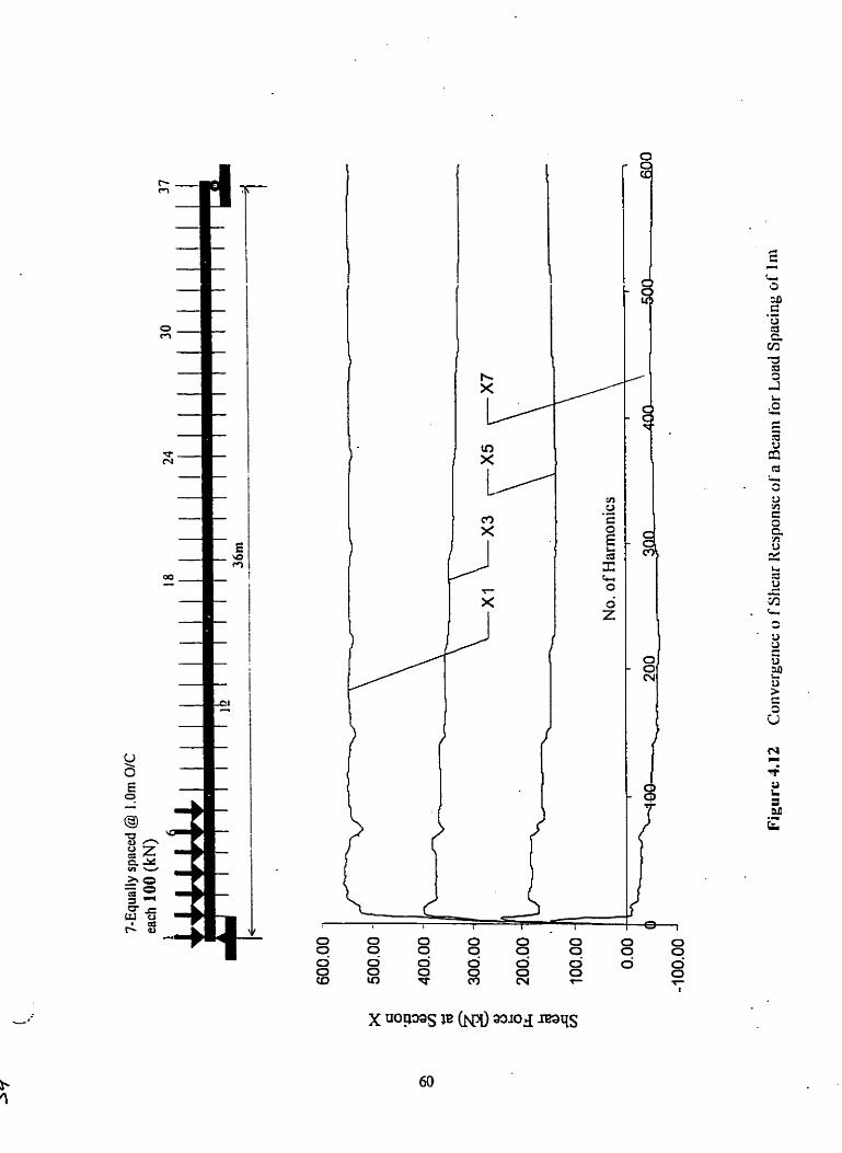
Convergence O f Shear Response of a Beam for Load Spacing of l m
Convergence of Shear Response of a Beam for Load Spacing of 3rn
Convergence of Shear Response of a Beam for Load Spacing of Sm
Convergence of Moment Response of a Beam for Load Spacing of l m
Convergence of Moment Response of a Beam for Load Spacing of 3m
Convergence of Moment Response of a Beam for Load Spacing of 5m
Shear Response of a X p a n Beam for Truck Load
Convergence of Shear Response of a 3-Span Beam for Truck Load
Moment Response of a 3-Span Bearn for Truck Load
Convergence of Moment Response of a 3-Span Beam for Truck Load
Bridge Deck Plan, Cross-Section and Loads
5D Plot of Longitudinal Shears in Bridge Girders [Standard Case a =
0.101
Longitudinal Girder Shear Distribution (Typical Slab-Girder Bridge)
Convergence of Longitudinal Girder Shear (Typical Slab-Girder Bridge)
3D Plot of Longitudinal Moments in Bridge Girders [Standard Case a =
0.1 O]
Longitudinal Girder Moments Distribution (Typical Slab-Girder Bridge)
Convergence of Longitudinal Girder Moments (Typical Slab-Girder
Bridge)
Bndge Geometry and Load Configuration
Distribution of Longitudinal Shear
Convergence of Longitudinal Shear in Girders
Distribution of Longitudinal Moments in Girden
Convergence of Longitudinal Moments in Girders
Longitudinal Shear Distribution in Girders [Torsionally Soft Bridge u =
0.061
Convergence of Longitudinal Shear Distribution in Girders [Torsionaily
Soft Bndge u = 0.06]
Longitudinal Girder Moment Distribution [Torsionally Soft Bndge a =
0.061
viii

Figure 437
Figure 4.38
Figure 4-39
Figure 4.40
Figure 4.41
Figure 5.1
Figure 5.2
Figure 53
Figure 5.1
Figure 5.5
Figure 5.6
Figure 5.7
Figure 5.9
Figure 5.9
Figure 5.10
Figure 5.11
Convergence of Longitudinal Girder Moments [Torsionaily Soft Bridge a
= 0.061
Longitudinal Shear Distribution in Girden [Torsionally Stiff Bridge a =
0.061
Convergence of Longitudinal S hear Distribution in Girders [Torsiondly
Stiff Bridge a = 0.061
Longitudinal Moment Distribution [Torsionaily S tiff Bridge a = O 201
Convergence of Longitudinal Girder Moments [Torsionally Stiff Bridge a
= 020]
Bending Moments: (a) Free Bending Moment Diagram; (b) Bçnding
Moment Diagram düe to first Harmonic
Bending Moment due to first Harmonic: (a) Moments Retained by the
Middle Girder: (b) Moments Passed on to Outer Four Girders: and (c)
Moments Passed on to Outer Four Girders Deducted fiom the Free
Moment Diagram
Cornparison of Mid-Span Girder Moments Obtained by the Manuai and
Computer-Based Semi-Continuum Methods
Single Span Girder Bridge [Single Load]
Transverse Distribution of Longitudinal Moments In Girder Bridge
[Single Span & Single Load]
Longitudinal Moment Distribution In E.uternally Loaded Girder [Single
Span Rr Single Load]
Transverse Distribution Of Longitudinal Shears in Girder Bridge [Single
S p a & Single Load]
Longitudinal Shear Distribution in Extemally Loaded Girder [Single Span
& Single Load]
Single Span Girder Bridge under One Line of OHBDC Tmck Load
Transverse Distribution of Longitudinal Moment in Girder Bridge [Single
Span & Truck Load]
Longitudinal Moment Distribution in Extemally Loaded Girder [Single
Span & Tmck Load]
Figure 5.12
Figure 5.13
Figure 5.14
Figure 5.15
Figure 5.16
Figure 5.17
Figure 5.18
Figure 5.19
Figure 5.20
Figure 5.2 1
Figure 5.22
Figure 5.23
Figure 5.21
Figure 5.25
Figure 5.26
Figure 5.27
Figure 538
Transverse Distribution of Longitudinal Shears in Girder Bridge [Single
Span & Truck Load]
Longitudinal Shear Distribution in Extemally Loaded Girder [Single Span
& Truck Load]
Two-Span Girder Bridge under One Line of OHBDC Truck Load
Transverse Distribution of Longitudinal Moment in Girder Bndge [2-Span
% T ~ x k h 3 d ]
Longitudinal Moment Distribution in Extemaily Loaded Girder [î-Span &
Tmck Load]
Transverse Distribution of Longitudinal Shear in Girder Bndge [ZSpan &
Tmck Load]
Longitudinal Shear Distribution in Extemally Loaded Girder [2-Span &
Tmck Load]
Definition of ELSS for Slab Bridges
Single-Span Slab Bridge [Single Load]
Transverse Distribution of Longitudinal Moments in Slab Bndge [I-Span
& Truck Load]
Longitudinal Moment Distribution in Exemally Loaded Slab S t i ~ p [2-
Span & Truck Load]
Transverse Distribution of Longitudinal Shear (V,) in Slab Bridge [Single
Load & Single Span]
Longitudinal Shear Distribution in Extemaily Loaded Slab Sfri [Single
Load & Single Spm]
Single-Span Slab Bridge under a partial hne of wheel of OHBDC . +
Puck
Transverse Distribution of Longitudinal Moment (Mx) in Slab Bridge
[Truck Load & Singie Span]
Longitudinal Moment Distribution in Extemaiiy Loaded Slab Strip [Tmck
Load & Single Span]
Transverse Distribution of Longitudinal Shear in Slab Bridge pmck Load
& Single Span]
Figure 5.29
Figure 5.30
Figure 5.31
Figure 5.32
Figure 5.33
Figure 5.34
Figure 6.1
Figure 6.2
Figure 6.3
Figure 6.4
Longitudinal Shear Distribution in Externdy Loaded Slab Strip [Truck
Load & Single Span]
Two-Spa Slab Bridge under a Partial Line of Wheel of OHBDC Tmck
Transverse Distribution of Longitudinal Moments (Mx) in Slab Bridge
[Truck Load & Two Span]
Longitudinal Moment Distribution in Externaily Loaded Slab Strip [Truck
Lsad & X p a n ]
Transverse Dlszibution of Longitudinal Shear (V,) in Slab Bridge [Truck
Load & 2-Span]
Longitudinal Shear Distribution in Externally Loaded Slab Strip [Truck
Load & 2-Span]
Schematic Representation of the ShearMoment Computations in
Onhotropic Plate Method
Flow Chart for Program PLAT0
Typical Bridge Deck with Edge Beams
Flow Chart for Progam EDGE

List of Tables
Table 2.1
Table 4.1
Table 4.2
Table 5.1
Table 5.2
Table 5.2.1
Table 5.3
Table 5.3.1
Table 5.4
Table 5.4.1
Table 5.5
Table 5.5.1
Table 5.6
Table 5.6.1
Table 5.7(a)
Table 5.7@)
Table 5.8
Table 5.9
Table 5.10
Table 5.1 1
Table 5.12
Table 5.13
Table 5.14
Table 5-15
Factors afTecting a parameter
No. of harmonies required for 99% convergence in beams
No. of harmonies required for 99% convergence in bridges
Values of Mx obtained by PLATO at x = 15 m, in kN.m/rn
Values of V, obtained by PLATO at x = 0, in k N / h
Vx in ELG using Hastening Technique
Values of Mx obtained by PLATO at x = 15 m, in kN.m/m
Mx in ELG using Hastenhg Technique
Values of V, obtained by PLATO at x = 0, kN/m
Y, in ELG using Hastening Technique
Values of hf' obtained by PLATO at x = 15 rn, in kN.m/m
Mx in ELG using Hastening Technique
Values of Y, obtained by PLATO at x = 7.5 m, kN/m
V, in ELG using Hastening Technique
Aspect Ratio Effect: Slab Bridge Response for Longitudinal Moments
( M x )
Aspect Ratio Effect: Slab Bridge Response for Longitudinal Shears (YK)
Patch Size Effect: Slab Bridge Response for Longitudinal Moments (Mx)
Patch Size Effect: Slab Bridge Response for Longinidinal Shem (V,)
Sumrnary of the Effects of Aspect Ratio (WL) on EMS
Sunimary of the Effects of Load Width v on ELSS
PLATO results for mid-span M, in a Single Span Slab Bndge [u = O]
PLATO results for mid-span Mx in a Single Span Slab Bndge [u = 0.31
PLATO results for mid-span Y, in a Single Span Slab Bndge [u = O]
PLATO results for mid-span Y' in a Single Span Slab Bridge [u = 0.31
Table 5.18 Values of Mx obtained by PLATO at x = 5 rn
Table 5.18.1 M, in ELSS using Hastering Technique
xii

Table 5.19
Table 5.19.1
Table 5.20
Table 5.20.1
Table 5.21
Table 5.21.1
Table 5.22
Table 5.22.1
Table 5.23
TabIe 5.23.1
Table 5.24
Table El(a)
Table El@)
Table E2(a)
TabIe E2@)
Table E3(a)
Table E3@)
Table E4(a)
Table E4@)
Table Fl(a)
Table FI@)
Table Pl
Values of Vx obtained by PLATO at x = O
Y, in ELSS using Hastening Technique
Values of M, obtained by PLATO at x = 5 rn
hfx in ELSS usîng Haçtening Technique
Values of V, obtained by PLATO at x = O
V, in ELSS using Hastening Technique
Values of Adx obtained by PLATO at .r = 5 m
M, in ELSS using Hastening Technique
Values of V, obtained by PLATO at x = 2.5 rn
V, in ELSS using Hastenhg Technique
S m a r y of % Accuracy using Hastenhg Technique in Girder and Slab
Values of Fx obtained by PLATO at x = O m, kN/m [Load size: O. 25m x
0.2m ]
Y, in ELG using Hastening Technique
Values of Y, obtained by PLATO at x = O m, M m [Load size: O.25m x
O. 4m j
Y, in ELG using Hastening Technique
Values of V, obtained by PLATO at x = O m, kN/m [Load size: 0.25m x
O. 6ml
V, in ELG using Hastening Technique
Values of V, obtained by PLATO at x = O m, kNlm [Loadsize: O.Z.5rn x
I.Omj
Y, in ELG using Hastening Technique
Values of V, obtained by PLATO at r = 7.5 rn, kN/m
Y, in ELG using Hastening Technique
Girder bridge properties
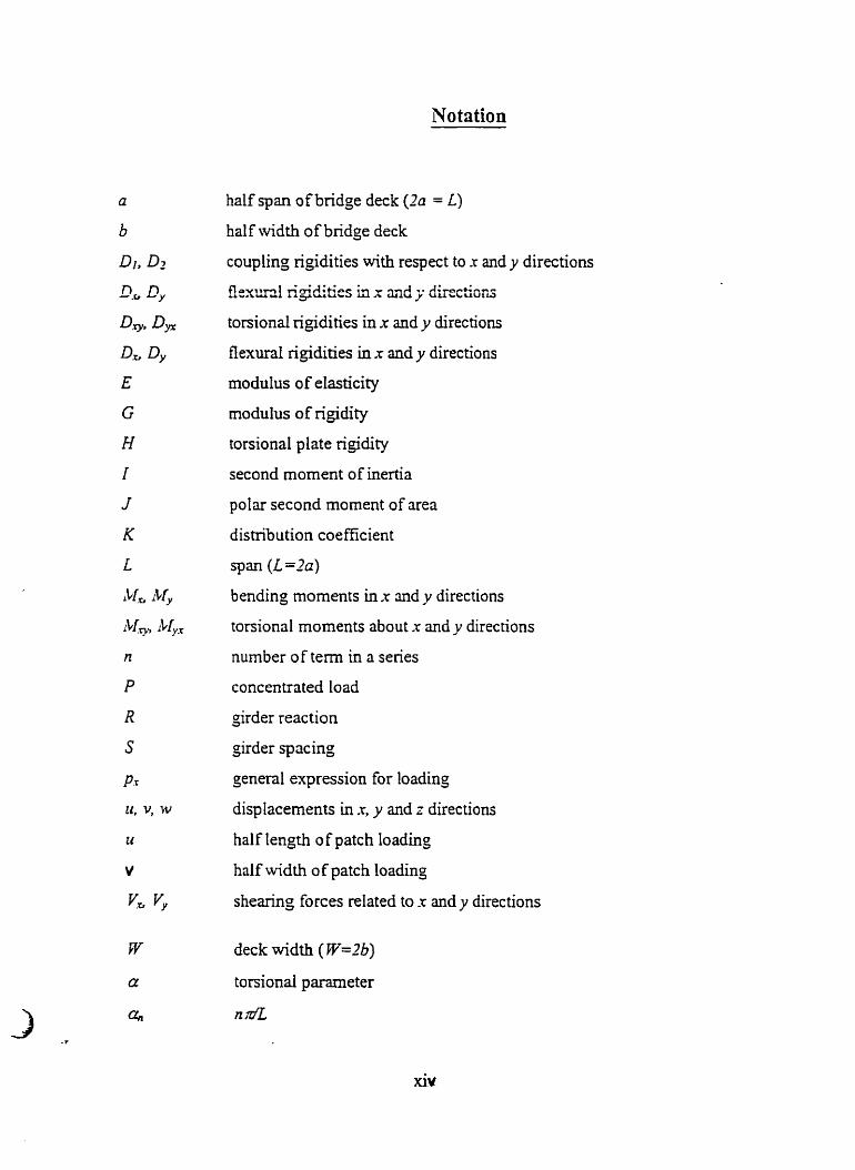
Notation
half span of bridge deck (20 = L)
half width of bridge deck
coupling rigidities with respect to r and y directions
9mm1 rigidities in x and y dir-cG b C ~ O T ~ S
torsional rigidities in x and y directions
Bexural rigidities in .T and y directions
modulus of elasticity
modulus of ngidity
torsional plate rigidity
second moment of inertia
polar second moment of area
distribution coefficient
span (L=Za)
bending moments in x and y directions
tonional moments about x and y directions
number of term in a series
concentrated load
girder reaction
girder spacing
general expression for loading
displacements in .Y, y and z directions
half length of patch loading
half width of patch loading
shearing forces related to x and y directions
deck width ( W=2b)
torsional parameter
n d
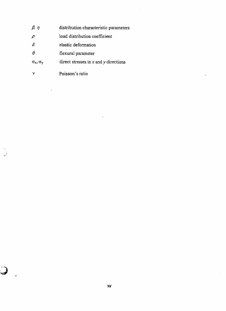
distribution characteristic parameters
load distribution coefficient
elastic deformation
flexural parameter
direct stresses in .Y and y directions
Poisson's ratio

Scope and Objectives
1.1 Statement of Problem
The rigorous methods for analyzing bridge decks generally fdl into two categories: the
finite element methods using discrete idealization, and others using continuum
idealization. The finite element methods require discretized modeling of the structure and
usually generate large volume of output data. Also, the finite element prograrns require
extensive input. In the other methods of bt-idge deck analysis, the actual deck structure is
idedized as a semi-continuum or equivalent orthotropic plate. The desired structural
responses such as shears, moments and deflections are then obtained from series
solutions denved kom classical theories of plate bending. The series solutions are
relatively slow in convergence and significantly large number of tems of the series are
usuaily required to obtain accurate responses. It is desirable to develop techniques that
could hasten the convergence of these series solutions.
1.2 Research Objectives, Scope, and Methodology
The orthotropic plate method for rectangular plates supported on two opposite edges
(Cusens and Pama, 1975) is based on a series solution. The convergence of this method is
slow especially for shears. As many as 50 harrnonics may be required to achieve WNally
1

complete convergence. The orthotropic plate method is currently being incorporated in a
pro-, called PLATO.
The serni-continuum method of analysis (Jaeger and Bakht, 1989), incorporated in a
program called SECAN, is also based on a series solution. However, the use of a novel
technique has enwed that its results converge very quickly. Only five hannonics are
often sufficient to obtain vimially cornpiete convergence.
The purpose of the curent project is to demonstrate numericdly that the technique of
hastening convergence employed in the semi-continuum method c m also be applied to
the orthotropic plate method. In order to achieve this objective, the following research
methodology was adopted. Firstly, the convergence of beam responses was studied using
the harmonic ~ialysis technique incorporated in a spreadsheet program. Similarly, the
convergence of responses in typicai slab-on-girder bridge structures was studied using the
semi-continuum method also incorporated in spreadsheet programs. The program
SECAN incorporates the quick convergence scheme and, therefore, could not be used
directly to study the convergence of responses in bridge structures. The spreadsheet
modules prepared for this study include the d e t e d a t i o n of longitudinal responses.
These responses were also evaiuated for tonionally soft and flexurally stiff bridges.
The quick convergence technique of the semi-continuum method was then numericdly
demonstrated for the orthotropic plate method of andyzing slab-on-@der and slabs
bridges with various loading configurations and support conditions.
3 -

ï h e scope of this study was limited to right bridges, i.e., bridges with zero degree of
skew. A second objective of this study was to formulate a procedure for determining
longitudinal moments in the edge beams of slab-on-girder and slab bridges. The
computation scheme was successfully incorporated in the program PLATO, and the
resulting modified program narned EDGE.
1.3 Thesis organization
Chapter two brietly reviews the semi-continuum and orthotropic plate methods of bridge
deck analyses. The limitations and appropriate use of these methods are also bnefly
discussed.
In chapter three. spreadsheet prograrns are discussed for beams and bridge structures
including single and multiple spans and with various loading configurations. These
programs use harmonic series solutions.
Chapter four snidies the convergence of structural responses in beams and bndge decks
with single and multiple spans and with various load configurations. Convergence of
structural responses is evaluated at only those locations where convergence is rnost
dificult. Convergence is being sought as an academic exercise. The snidy dso covers
the effects of tonional and flexural stifiesses on the convergence of longitudinal
responses in slab-on-girder bridges

Chapter five discuçses the hastening of convergence technique for the semi-continuum
method and demonstrates nurnerically that the technique c m also be applied to the
orthotropic method of bridge deck analysis. The study includes single and multiple span
slab-on-girder bridges and siab bridges for various load configurations.
Chapter six reviews the formulation scheme of the orthotropic plate method incorporated
in the program PLATO. It M e r discusses moment computations in edge beams of slab-
on-girder and slab bridges. Finaily, it explains the incorporation of edge beam moment
computations in the program PLATO. The resulting pro- is called EDGE.
Chapter seven surnmarizes the conclusions derived from this study and provides
recornmendations for future research.

Chapter 2 Bridge Deck Analysis
2.1 Introduction
The behavior of a bndge deck is usually govemed by its structural form and geometry.
Bridge deck structural form may vary widely from one structural type to another.
However, this chapter discusses the behavior and analysis of shallow-type structures
including voided-slab, solid-slab. and slab-on-girder bridges. Two different methods of
analyzing thesr bridges are discussed. The application of these methods to other forms of
btidge decks including and multicell box-girder type bridges is also discussed.
The modeling of a typical bridge deck involves two phases: the idealization of wheel
loads, and the transformation of the deck structure to an equivalent mathematical mode1
representing its physical behavior. In the two methods under consideration, wheel loads
are transformed into equivalent continuous forms by using hannonic or Fourier series.
The response of deck structure at a given point is then obtained using classical bending
theones of plates and beams.
The numericd methods reviewed in this chapter are based on series solution and have
clear application to computation by means of digital cornputers. A novel approach s h d
be developed later to achieve quick convergence of results using series solution.

2.2 The Semi-continuum Nlethod
The serni-continnum method of load distribution analysis of bridges involves
representation of wheel loads by harmonic senes and the idealization of deck structure
by discrete longitudinal mernben and a transverse continuum.
Hendry and Jaeger (1955) first used this method for analyzing bridges with negligible
torsïonless stifhesses. Later, Bakht and Jaeger (1 985) developed a more generalized
form of this method to analyze bridges with torsional stiftness in both longitudinal and
transverse directions. Before briefly reviewing this method, the h m o n i c analysis of the
wheel loads and its significance shall be reviewed in the following section.
2.2.1 Wheel Loads Idealized as Harmonic Loads
A point load P on a simply supported beam of span L, c m be represented as a
continuous load of intensity p,, using following expression:
where x is measured f b m the left hand support and c is the distance of the load fiom the
The point load is therefore equivalent to the s u - of infinite number of distributed loads
given by the above equation. An important feature of loads represented by a harmonic

series is that the deflected shapes of any girder under the loading represented by any
term of the series has the same shape as of the loading itself. As a result the ratio of
deflections of any two beams of abridge at any transverse section remains constant
throughout the çpan of the bridge. Because of this property of h m o n i c loads, only a
transverse slice of the deck structure can be solved for load distribution in the bridge
deck.
Once the given point load is transformed into equivalent harmonic Function then using
- El* leads to the following srnail-deflection beam theory equation, p,,, - d x i '
expressions for shewing force, bending moment and dope.
d 3 0 d'o do ......................... V,,, = EI- 1 , = EI- O,,, = EI- ..[2.2] d x 3 ' d x' ' d x
The free response, i.e., response oFa &der if it were to sustain ail applied loads without
sharuig with other girders is therefore obtained by successive integration of the p,
equation.

2.2.2 Deck Structure Idealized as Semi-continuum Mode1
In the serni-continuum method, the longitudinal bending and twisting properties of the
deck structure are idealized as being concentrated into a number of longitudinal elements
of negiigibie dimensions, whiist rhe transverse benciing and twisting propenies are
uniformly distributed arnong an intinite number of transverse bems which fom the
transverse medium. This way the physical properties of the slab-on-girder type bridges
are closely represented by the mathematical ideaiization.
A partial cross-section of a typicai girder-slab bridge s h o w in Figure 2.l(a). The
behavior of the transverse medium cm be represented by a beam of unit width as shown
in Figure 2.l(b). The extemai load is shared between the girden as Ri, RI, and Rn.
Further. this transverse element expenences deflections &, & and & and rotations h, &,
and at its respective girder locations.
The response of this system cm be modeled as a system of linear and rotational springs
as shown in Figure 2.2. In this figure, vertical and circular springs represent the flexural
and torsionai rigidities &, Or of the girders, and the horizontal spring represents the
torsional rigidity Yr of the transverse medium. These rigidities for various harmonies n
can be computed as,

Load
4 Girder Spacing r A k Girder Spacing -B
R 1
Figure 2.1 Bending of a Transverse Slice of the Deck (a) Actual Structure @) Response of the Transverse Slice
The systern of forces shown in Figure 2.1 can be solved for the unknown girder reactions
Ri, Rz, through &, and rotations b, h, through q& using equations of equilibrium and
compatibility. The details of solving various equations for the unknowns have been

provided by Bakht and Jaeger (1989). The girder reactions and torsional moments are
expressed in terms of distribution coefficients p(,),,, for longitudinal moments and shears
in girders, and distribution coefficients p*(,),,, for longitudinal twisting moments in
girders. This process of obtaining distribution coefficients is repeated for every
individual harmonic effect.
Transverse Torsional Rigidity of Slab
Flexural Rigidity of
Figure 2.2 Equivalent Spring Model of the Transverse Element
The acnial response in a given girder is then obtained by nunming the individual
responses for successive harmonies. Therefore, the hmonic response at any given
section 'x ' is given by:

The total response can be obtained by s u d g the individual responses as given below,
2.2.3 The Manual Method
Jaeger and Bakht (1989) have derived expressions and drawn curves for the distribution
coefficients p ( , ~ for specific bridge geometry and load position. The distribution
coefficients for a given case are related to characterizing panmeters P and q defined as:
Where, L and S are respectively the span of the bridge and the spacing of gird&. Jaeger
and Bakht (1989) have also proposed that for loads acting between girderb[ocations,
equivaient simply supported beam reactions should be computed in using the above
manual method of determining load distribution in girders of slab-un-&der bridges.

For a typical five-girder bridge with equivalent loads acting on each girder, the
expressions for the distribution coefficients are given by Jaeger and Bakht (1989). The
load distribution coefficients are computed for individual load cases i.e., load acting on
&der 1 only and so on. The total longitudinal response for a particular &der for a given
harmonic is then obtained by d g the individual Load contributions. This is
illustrated in Figure 2.3.
Figure 2 3 Illustration of the Manual Method for Multiple Loads
The load transfened to girder 1, for instance, is given by;

Where p, is the distribution coefficient for girder i due to a unit load on girder j. To
compute &der reactions distribution coefficients are calculated for each load case.
Moreover, for every single harmonic n, factors P and q are re-computed and a11
distribution coefficients are also computed accordingly to compute load transfer
component for the respective hamonic. Although the method is called 'Manual', the
calculations are too lengthy for manual computations with a large number of hamionics.
In chapter three, the equations for load distribution in a five-girder bridge (Bakht and
Jaeger) shall be used to develop spreadsheet modules for obtaining longitudinal shear and
moment responses of slab-on-girder bridges.
2 3 The Orthotropic Plate Method
In the orthotropic plate method of bridge analysis, the actual deck stnicture is idealized as
an equivalent orthotropic plate. The response of the structure is obtained using elastic
theory of thin plate bending. An orthotropic plate is defined as an equivalent plate having
different elastic properties in two orthogonal directions. A brief histokal review of the
developments in plate bending theories and orthotropic plate method is given in the
following sections.
2.3.1 Idealization of WheeI Loads

In an orthotropic plate, the responses are disconthuous under a point load. It is desirable
to avoid point loads and represent concentrated loads as patch load. Cusens and Pama
(1975) have used rectangular patch loads havhg a length u and width v. A uniformly ..
distributed load of .partial length u on a simply supported beam is represented by the
following equation.
SP " nnc n m . nxu P(~)~=- ~ s i ~ y n - s l r t - .......... ....... -..... ..... ...... ... . ... .......... [2.19]
n=I L L
2.3.2 Ideaiization of Deck Structure
In orthotropic idealization of bridge deck, the longitudinal flexural and tonional rigidities
are assurned uniformiy distributed across the bridge length and width. It is therefore
important thst the acnial bridge should have a reasonable number of longitudinal beams
to yield reasonably uniform distribution of flexural and torsional ngidities in transverse
direction. As a general rule, Cusens and Pama (1975) have suggested a minimum of five
longitudinal girders in treatuig the achial deck structure as an equivalent orthotropic
plate.
The various plate rigidities in a rectangular orthotropic plate are defined as follows:
9r Longitudinal flexuml rigidity per unit width
Dy Transverse fiexural rigidity per unit length
D, Longitudinal torsional rigidity per unit width
D, Transverse torsional rigidity per unit length

DI Longitudinal couphg rigidity per unit width
Dz Transverçecouphgngidityperunitlength
These rigidities are functions of the elastic properties of the deck material and the
interaction between deck slab and individual beams. Standard expressions for these
rigidity parameters for various types of bridge deck structures are given in the standard
text books, and also in the OHBD Code (1993).
2.3.3 Plate Bending Theories: Bistoncd Review
in the theory of plate behavior, the first analytical work was published by L. Euler in
1766 who perfonned dynamic analysis of rectangular and circular elastic plates using the
analogy of two systems of stretched strings perpendicular to each other. Navier (1785-
18361, is also considered as the real originator of the modem theory of elasticity. He
derived the di fferential equation of rectmgular plates with flexunl resistance. His various
scientific activities included the solution of various plate problems. For the solution of
certain boundary value problems, he introduced an 'exact' method which transfomis the
differential equations into algebraic equations. Navier's method is based on the use of the
trigonometri series introduced by Fourier in the same decade. This so called forced
solution of differential equations yields mathematically exact solutions of the Navier's
type plate.

G. R. Kirchhoff (18244887) is considered the founder of the extended plate theory that
takes into account the bending and stretching effects. He also pointed out that there exists
only two boundary conditions on a plate edges and also considered the large deflection
effects.
Russian scientists also made significant contribution in solid mathematical theories.
However, because of the existing language barrier, the Westem world was slow to
recognize and make use of these Russian achievements. It is to Timoshenko's credit that
the attention of the Westem scientists was graduaily directed toward the Russians
research in the field of the theory of elasticity. Among Timoshenko's numerous
important contributions are solution of circular plates considering large deflections and
the formulation of elastic stability problems.
The developments in shipbuilding and the modem aircratt industry provided another
strong impetus toward more rigorous analytical investigations of the plate problems.
The solution ofrectangular plates with two simple and parallel supports was formuiated
by Levy in the late 19'~ century. The advancements of classical techniques have
permitted new insight and new techniques in the numerical solution of cornplex plate and
shell problems in an economid way. The recent trends in the development of the plate
theories are characterized by heavy reliance on hi&-speed cornputen and by the
introduction of more ngorous theories.
Idealization of reinforced concrete bridge decks as an equivalent orthotropic plate was
first formulated by Huber (1914). This was followed by Guyon (1946) who used the
method to analyze a torsionless deck. h4ismmt (1950) sdaded Ifie medmd to inchde the tomarial
stiffness of the deck. Since that tirne, the developments in classical plate solutions have
continued through the efforts of Jaeger, Cusens, Pama, and many othes.
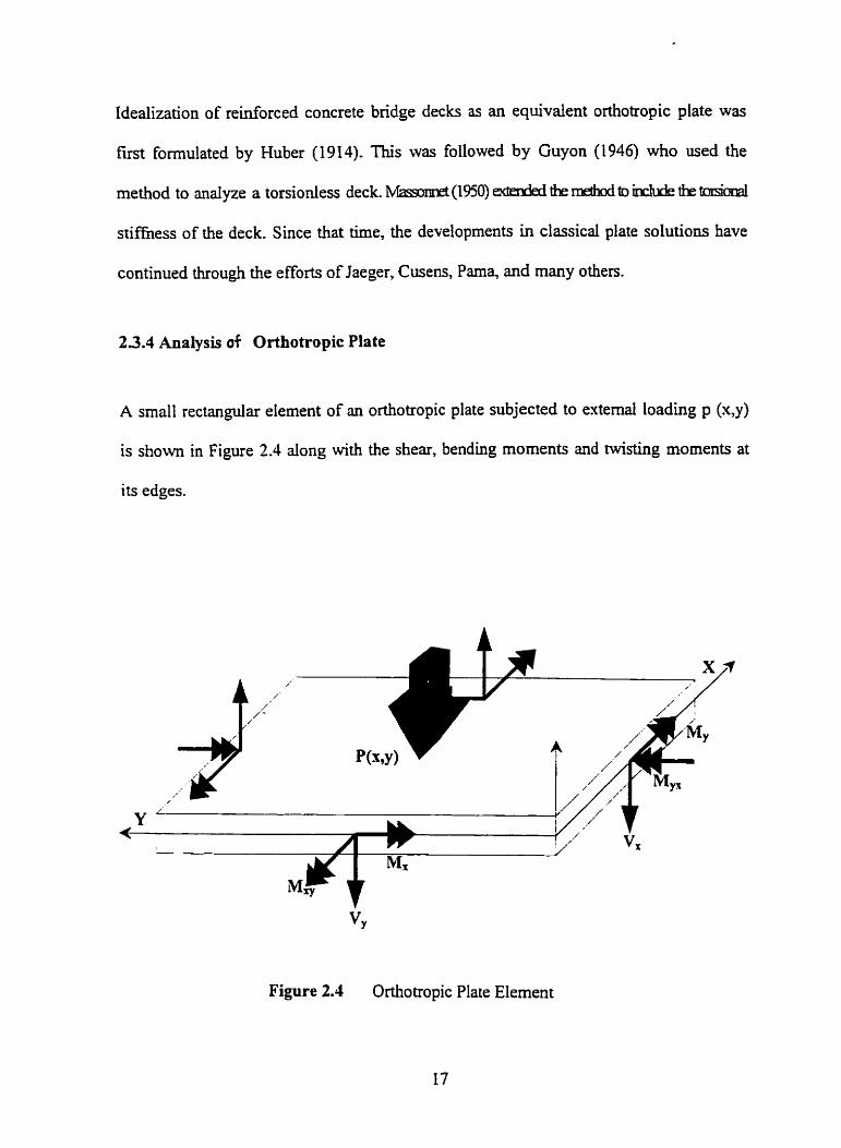
23.4 Analysis of Orthotropic Plate
A small rectangular element of an orthotropic plate subjected to extemal loading p @,y)
is s h o w in Figure 2.4 dong with the shear, bending moments and twisting moments at
its edges.
Figure 2.4 Orthotropic Plate Element

Using Kirchhoff s hypothesis and neglecting axial stress effects, three diensional plate
problem reduces to two dimensions and the expressions for bending and shearing stresses
can be readily obtained as follows.
The bending moments per unit width in the x and y directions are Mr and iCl, respectively
and the twisting moments are denoted by LM, and 1 4 ; the expressions for these
responses are given below,

Consideration of the equilibrium of moments and forces acting on the elernent s h o w in
Fimire - 2.4 and the substitution of above expressions of moment resultants give fo!bwing
differential equation of the orthotropic plate,
The shearing forces V, and V, c m be expressed in tems of the defection o as Jiven
below,
The solution of the non-homogeneous differential equation of orthotropic plate can be
obtained by adding particular and homogeneous parts after considering the effects of
extemai loads and boundary conditions at plate ends. The solution of this fourth order
di ffer ential equation is the deflection expression derived fiom particdar and
homogeneous parts. The precise solution depends upon the relative e e s s parameters.

Cusens and Pama (1975) have s h o w that the general f o m of this solution can be
expressed as,
n e coefficient *lEi is cdled the distribution coeficient md is a function of the flexural
and torsional ngidities, the bridge geornem, and position of the load.
2.4 Characterizing Parameters a and 0
The goveming differential
Jaeger ( 1985).
equation in section 2.3.4 had been modified by Bakht and
Where, x ' and y ' are dimensionless quantities defined as x '= x / L and y ' = y / b (b=W/2),
and a and 8 are dimensionless characterizing parameten and are given by following
rquations.
n ie parameter a physically represents the torsionai stifYness of the
f l e d stiffhess. A higher value of a indicates a higher torsional
deck relative to its
resistance and vice
versa. The 0 parameter, on the other hand, represents the longitudinal flexural stiffness
relative to the &ansverse Bexural resistance. A higher value of 0 shows a bridge having
short span or wide p l d o m . 20

relative to the transverse f l e d resistance. A higher value of 0 shows a bridge havhg
short span or wide planf'orm.
The effect of coupling rigidities Di and D2 in girder bridges is usually small and c m be
neglected for computing a and 8 parameters. Further, the influence of key variables
including moments of inertia of the girder 1. tosional inertia of the girder J. girder spacing
S and slab thickness t on a and 0 parameters can be studied by expressing the torsional
and flexurai rigidities in equations 2.32 and 2.33 in terms of 1, J, S, t, and constants E and
G.
For slab-on-girder bridges, Baklit and Jaeger (1985) have proposed a lower and upper
bounds (practical) of a value of 0.06 and 0.20, respectively. Slab bridges (or isotropic
plates) have a=l . Values of a above 1 .O correspond to multi-ce11 and rnulti-spline box-
girder type bridges. A conceptual representation of a and 0 for typical bridges is shown
in Figure 2.5.
0.0 1 o. 1 1 .O
Figure 2.5 Practical Range of a, 0 Values
3 1

2.41 Effect of a Parameter on Structural Response of Slab-on-Girder Bridges
The structural response of slab-girder bridges is sipficantiy affected by its load
distribution characteristics that are functions of f l e d and torsional rigidities of the
bridge. For instance, in a flexurally stiff bridge deck the s t E girders would a m c t more
loads and vice versa. in order to study the influence of bridge deck rigidities, or load
distribution characteristics, on the convergence of various responses, a large number of
slab-pirder bridges of various flexurai and torsional rigidities shouid be anaiyzed,
requiring an enormous amount of work. On the other hand. the a parameter concept
discussed earlier c m be used to reduce the arnount of computations. Thus, instead of
analyzing a large number of bridges with various rigidities, only three bridges can be
considered for midying the effect of bridge deck rigidities on convergence of various
responses, these bridges being (1) a typical bridge with a = 0.10. (2) a torsionally soft
bridge with a = 0.06, and (3) a toniondly stiff bridge with a = 0.20.
Since the actual bridge deck anaiysis requires bridge deck properties such as 1, J, t, and S
as defined earlier, it is essential to obtain those values which correspond to desired values
of a. Obviously. a large number of combinations of these values can yield the sarne a
value. To make the procedure simple, the impact of different values of 1, J, t, and S on a
values should be observed so that arnong the given variables the ones which a e c t the a
parameter most should be selected as prime variables. In other words, instead of using
various possible combinations of 1, J, t, and S for obtaining a = 0.06 and 0.20, the
variables which have less impact can be kept constant and the ones which affect the most
be varied to obtain desired a values. To achieve this objective, the individual effects of 1,

J. t, and S parameten on a values are obtained by using various arbitrary values. The
effect of variations in 1 values on a can be measured by varying 1 values between 0.5 to 4
(m4) and keeping other parameters (J, S, and t) constant. Similady, effects of variations in
J. S, and t on a are measured. The computations, performed using spreadsheet, are shown
in Table 2.1 and plotted in Figure 2.6. J and 1 can be selected as main variables and t and
S treated as typical constants.
These results show the Most dominant variable affecthg a value is the torsional moment
of intertia ( J ) of the girders. dso . as the slab-on-girder bridges with a girder spacing of
7.5m rarely have a slab thickness of over 400mm or less than ZOOrnm. because of which
the a-t plot is meaningless for slab thickness ofover 4OOrnm and less than 200m.m.
Table 2.1 Factors affecting a parameter
Constants: i Constants: S=Z.S,J4.025,t=û.24 I=2.39,5=û.025,t=0.24
Constants: S=t.S,f=2.39,t=0.24
Constants: S=2.5,5=0.025,1=2.39 1

Slab thickness, t (m)
Figure 2.6 Effect of Various Variables 1, J, S and t on a Values
O-"? 0.45
0.10 j 0.35
0.30 I 0.25 - 0.20 - 0.15 - 0.10 - 0.05 - Moment of Inertia, I (nt4)

After several trial m s , following combinations of J and 1 values were selected for
torsionally soft and torsionaily stiff bridges:
(1) Torsionally sofr bridge (PO. 06)
J-0.01 8m4, 1=3.32m4, (e0.24111, S=2 Sm)
(2) Torsionally stiyf bridge ( ~ 0 . 2 0 )
~=0.045m~, 1=1.45m4, (M).24rn, S=2.5m)
In the subsequent study of convergence response, these two extrerne types of slab-on-
girder bridges are studied by cornparhg their responses with a typical slab-girder bridge
for which a z 0.10.
Chapter 3 Spreadsheet Programs for
Harrnonic Series Solutions
3.1 The Role of Spreadsheets
Before the arrival of persona1 computers, engineering students were generally required to
leam the mathematical details behind most of the commonly used numencal methods.
They were often required to program these methods for large mainfnme computers using
general-purpose programrning language such as Fortran or Pascal. It was a lengthy and
tedious procedure.
During the 1980s, as personal computers becarne inaeasingly common and drmatically
more powerful, spreadsheets emerged as handy tools for tedious numerical calculations.
Though originally intended for canying out hancial calculations, the newer versions of
most commercial spreadsheets include provisions for implementing many of the
commonly used numaical methods and thus provide a very powerful computationd tool
for engineers and scientists. Most spreadsheets now have some numerÎcal methods built
directly into their command stnicture.

The series solutions of bridge deck analysis, as well as beam analysis methods, using
semi-continuum rnethod can be easily implemented within a spreadsheet sirnply by
making use of its basic features. Also, it provides excellent tools for displayhg output
data in various graphical formats.
Spreadsheet programs are prepared for simple and multiple span beams using harmonies
analyses techniques described earlier in chapter two. Spreadsheet programs are aiso
devebp to obtain longitudinal shear and moment responses of slab-on-girder bridges.
3.2 Spreadsheet Program for Simply Supported Beams
Consider a simply supported beam of span L with flexural rigidity EI. The harmonic
analysis technique explained in chapter two is used to cornpute various bearn responses
including shear, moment, and deflection at discrete locations along the span.
A schematic representation of the various operations of harmonic analysis using
spreadsheet is shown in Figure 3.1. The input panmeters include the sectional and
material properties and the number of harmonic terms n to be considered for analysis.
The input parameters for loads include its magnitude and location with respect to origin
at the left support. A -ve sign is used for loads acting upward
A total number of r +1 equi-distant reference sections are considered, and the responses
are calculated at each reference section, being X1, X2, etc. The computational algorithm


for each individual harmonic is then computed by using appropriated harmonic equation.
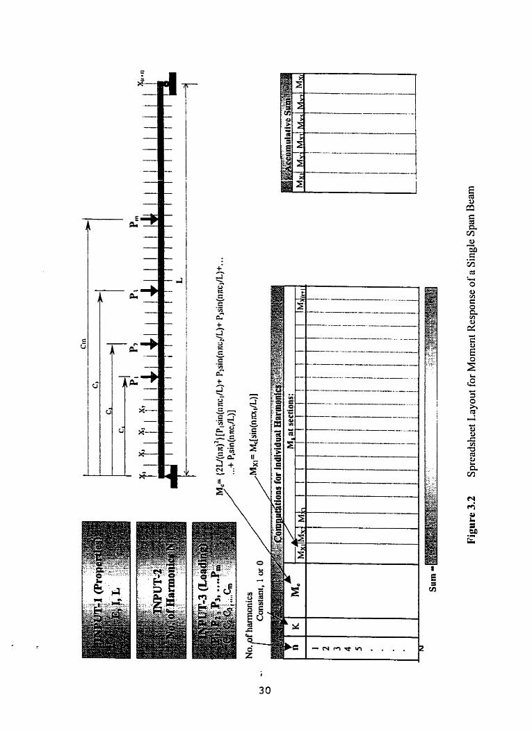
Figures 3.1 and 3.2 show respectively equations for shear and bending moments at
various sections for individual hannonics. To facilitate spreadsheet calculations, the
given hannonic equations for shear, moment, and deflection are modified as show in the
cornputationai box. The modified terms Y,, LM, and w, are then multiplied with
cos(nindl) or sin(nindL) to obtain Y', Mx, or w, at each of r + I sections.
The number of hannonics n required for the andysis can be any positive integer. The
responses for each individuai harmonies are summed to obtain the cumulative responses
at a given section.
To observe variations of a particular response at a selected section with respect to n, the
cumulative sum is obtained in a separate column, as shown in Figures 3.1 and 3.2. The
spreadsheet for shear response cm be modified by simply replacing (Unx) terni with
[2~/(nrr)~] and replacing c o s ( n ~ ) with s i n ( n d ) . Similar changes can be made to
obtain equivalent h m o n i c Ioad or deflection with the additional EI term in denominator.
3.3 Spreadsheet Program for Continuous Beams
Figure 3.3 shows a continuous beam with m number of spans. In order to perform
hannonic analysis for thïs beam, it is fint required to compute support reactions under
the applied loading. The beam is first anaiyzed using the spreadsheet developed for
deflection as a simply supported beam under the given loading, and deflection is
computed at each intermediate support location. Unit Ioads are then applied one at a time


at al1 support locations and deflections are computed. Intermediate support reactions are
then computed which wouid bring the bearns at these locations back to their original
positions.
Having obtained the unlaiown reactions at the intermediate supports, the beam with
intemediate supports c m now be analyzed by harmonic analysis as a simply supporteci
beam that is subjected to downward applied loading and usually upward reactions at
intermediate supports as computed above. The expressions for V, and bL are modified
accordingly to account for the effect of these reaction forces.
3.4 Spreadsheet Program for Longitudinal Response of Bridge Deck
The logical sequence of various operations required to perform step-wise calculations for
analyzing bridge decks using semi-continuum method is shown in Figure 3.4(a). The
schematic representation of various operations required for computing longitudinal
responses of the bridge is presented in Figure 3.4@). Charactenzing parameten P and q
are computed fiom the given bridge deck properties; these are later modified for every
harmonic.
The given wheel load is fint transformed into equivdent joint loads as equivded static
reactions. The loading input requires the magnitude and location of these equivalent joint
loads. The V,, as dehed previously for simple beam, is modified as Vc15, VCzc, and Vc3
for girder locations 1-5,2-4, and 3 separately. The load is shared by a given girder

rl Semi-continuum Method h
1 Point Load Idealization
1 Harmonic Transformation 1 I 2P ' nnc . nrrx
p, , , = - Esin-sui- L, t L I
c Beam Theory
d'a, PI,) = El- d f
da> Vix,= EI-
d x'
da, Q,,, = EI-
I - --
Free Response
1 Deck Structure 1 I Idealization I
Transformation into Semi- continuum Structure
S tiffness Parrimeters
Chancteristic Parameters
Transverse Distribution Factors 1
1 Corn pute Total Response
Figure 3 4 ~ ) Harmonie Andysis of Bridge Deck using Semi-Continuum Method

OHBDC Truck
WJ-UL3(
Equivalent Joint Load
1
/ Longitudinal Shear computations
(Girders CI & C5) (Typical for Girders G1 & C5)
VE= (VCl.d~ii mi) + VCI.~(PII PI*) + VSJ(PI)) }
Figure 3 4 h ) Spreüdsheei Lüyout for Longitudinal Response of a Bridge Deck

according to its load distribution coefficients. For instance, the Vc for girders 1 and 5 ,
considering similar loads on girder 1 and 5 , is given by
Expressions for girders 2 and 5, and girder 3 are derived similady. The expressions for
Ioad distribution coefficients, ps, for equally spaced girders, are developed,by Jaeger and
Bakht (1989), and are noted beiow.
Load on girder 2
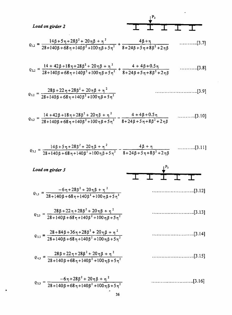
Load on girder 2
Lood on girder 3

The required Rspomes, being shear, moment, and deflection, are then obtained
separately for each girder at longitudinal sections 1 through r t l dong the bridge span.
Figure 3.4 shows spreadsheet computations for longitudinal shears in girders 1 and 5. The
spreadsheet program prepared for longitudinal analysis contains cornputations for girder
2 and 4. and &der 3.
nie totd reqonse at a &en section x for a specific girder is then obtained by summing t
individual responses. Using these results, a 3-D plot can be drawn using "~xcel's graphic
features to illustrate distribution of the longitudinal moments and shears of a particular
loading.
3.5 Transverse Response of Bridge Deck Slab
Consider a bridge deck loaded with loads positioned symmetrically about the longitudinal
axis of the bridge as shown in Figure 3.5. At a transverse section located at distance x, the
slab slice of unit width (6x4) is in equilibriurn under the given system of forces
including equivalent harmonic loads, girder reactions, and Cwisting moments, as shown in
Figure 3.6.
Figure 3.5 Tpical Bridge Plan and Loads
37
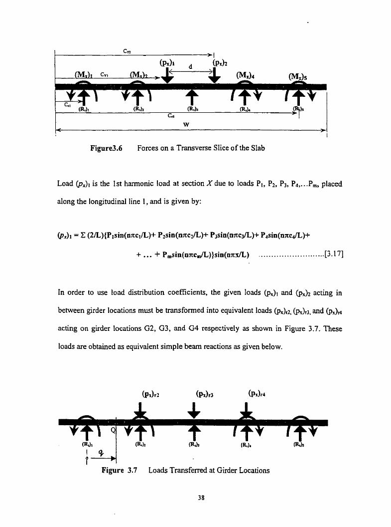
Figure3.6 Forces on a Transverse Slice of the Slab
Load @,) is the I st hamonic load at section X due to Ioads Pl , Pz, P3, Pd.. . .Pm, placed
along the longitudinal line 1, and is given by:
In order to use load distribution coefficients, the given loads @Ji and acting in
between girder locations m u t be transformed into equivalent loads (m)< (pJd, and (p&
acting on girder locations G2, G3, and G4 respectively as shown in Figure 3.7. These
loads are obiained as equivalent simple beam reactions as given below.
ms1
i Q Figure 3.7 Loads Transferred at Girder Locations
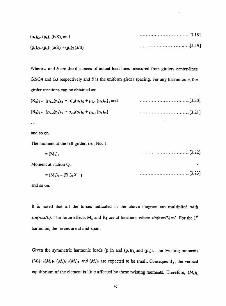
................................. [3. is]
................................ .[3. is]
Where a and b are the distances of actual Ioad lines measured fiom girders center-lines
GUG4 and G3 respectively and S is the uniforni girder spacing. For any hamonic n, the
girder reactions can be obtained as:
................................. x = ( ~ 1 2 @ r X 2 + P ~ J @ X ~ ) + P1.4 (h<h4}, and [3.20]
............................... (Rd2 = ( P ~ P J ~ z + P ~ J @ ~ X J + ~ 1 . 4 ( ~ x ) r 4 } ..p.- ' 1 I .
* * *
and so on.
The moment at the left girder, Le., No. 1,
= Wdi
Moment at station Q,
= (Md1 - CRiW 9
and so on.
It is noted that al1 the forces indicated in the above diagram are multiplied with
s i n ( n d ) . The force effects Mx and Ri are at Locations where s in(ndL) = l . For the 1"
harmonie, the lorces are at rnid-span.
Given the symmetric hmonic Ioads @,)r2 and and ( p , ) ~ , the tnnsting moments
(Mx)i .(A4Js, (iM,)z and are expected to be small. Consequently, the vertical
equilibnurn of the element is little affécted by these twisthg moments. Therefore, (MJI,

(M&, (1kf&, and are not considered in shear computations. It should be noticed that
the hvo system of forces sho~vn in Figures 3.5 and 3.6 are equivaient force systems.
However, for transverse shears and moments computations, the harmonic loads acting at
actual location shall be used (as s h o w in Figure 3.5).
A spreadsheet prograrn could be readily developed by using the above principles. In order
to keep the scope of the work within reasonable bounds, it was decided not to shidy the
transverse responses in the present study.
3.6 User Instructions for Spreadsheet Programs
There are hvo types of spreadsheets provided in the accompanying diskette: (1) beam
responses for shears and moments, (2) tonginidinai responses of bndge girders for shean
and moments. These spreadsheets are prepared using Microsof?@ Exce12000 for up to 10
harmonics. Responses for hmonics over 10 cm simply be obtained by using copy-paste
cornmands. The input boxes Tor loads, geometry, and stifhess properties should be
changed accordingly ro obtain structural response of a given beam or bndge deck for
required nurnber of harmonics.

Chapter 4 Convergence of Series Solutions
4.1 Introduction
Series solutions of bridge deck anaiysis using semi-continuum method or orthotropic
plate method usudly require several harmonic terms of the senes to achieve reasonable
accuracy. This chapter studies the effect of various factors thar intluence the convergence
of results of the senes solutions of the orthotropic plate method as discussed in chapter
two. First, responses being shear. moment. and deflections, of simple and continuous
beam structures are evaluated using spreadsheet programs discussed in chapter three. The
snidy is then extended to evaluate longitudinal moment and shear responses of slab-on-
girder bridges. Structural responses in beams and bndge decks are evaluated at locations
where convergence is rnost difficdt. Convergence is being sought as an academic
exercise. The parameten of convergence study include the effect of different load
configurations, relative location of the reference section with respect to loads, and the
effect of htroducing intermediate supports. Later, the study is also extended to include
torsionally sofi and torsionaily stiE bridges, using hypothetical extreme values of the u
parameter, discussed earlier in chapter two.
41

0 -
4.2 Convergence of Responses in Beams
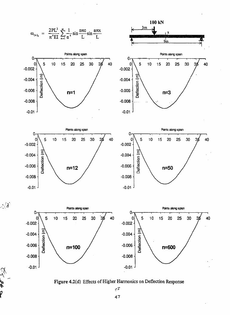
42.1 Response under single load
Consider a simply supported beam of span 9m, loaded with a single point load of 100 kN
at 3rn fiom left support, as show in Figure 4.1.
- Figurë4.1 - single sp& Beam Under Single Point Load
The point load can be represented as an equivalent distributed load of intensity p, (as
discussed in section 2.2.1). Using spreadsheet program for simple beam, discussed in
chapter three, the equivalent load for various hannonics, namely for n = 1,3, 12, 30, 100,
and 600, was calculated and is shown in Figure 4.2(a). In this and the subsequent figures
also, the beam length is divided hto 36 equal parts leading to 37 reference points. This
Figure shows that as the number of harmonies inneases the shape of the equivalent
harmonic load changes towards becoming a spike load.

y Points dong span
Points along span
200 1 I
-100 J Points along span
P o i n t s along span
Figure ~1.2@) Representation of a Point Load by Harmonic Senes

For the given beam, plots of shear, moment, and deflection are obtained for n = 1, 3, 9,
30, 100, and 600, and are shown in Figures 4.2(b), 4.2(c) and 4.2(d), respectively. These
results show hat the convergence of moments is faster than the convergence of shears.
n ie convergence is slower for higher derivatives of deflections. The study in subsequent
sections is, therefore, focused on the convergence behavior of shears and moments only.
The shear response of the same beam with load acting at 3m fkom left support is obtained
for various harmonics, n = 1 to 300. The combined responses for n = 1, 3, 7, 12, 18, 27,
40, and 70 are plotted in Figure 4.3. It can be seen that for n = 70, the shear diagram
closely represents the achiai shek diagram with a shear qf 66.6 + . kN and 33.3. kN at left
and right supports, respectively. The true values of these shears are very close to the
same.
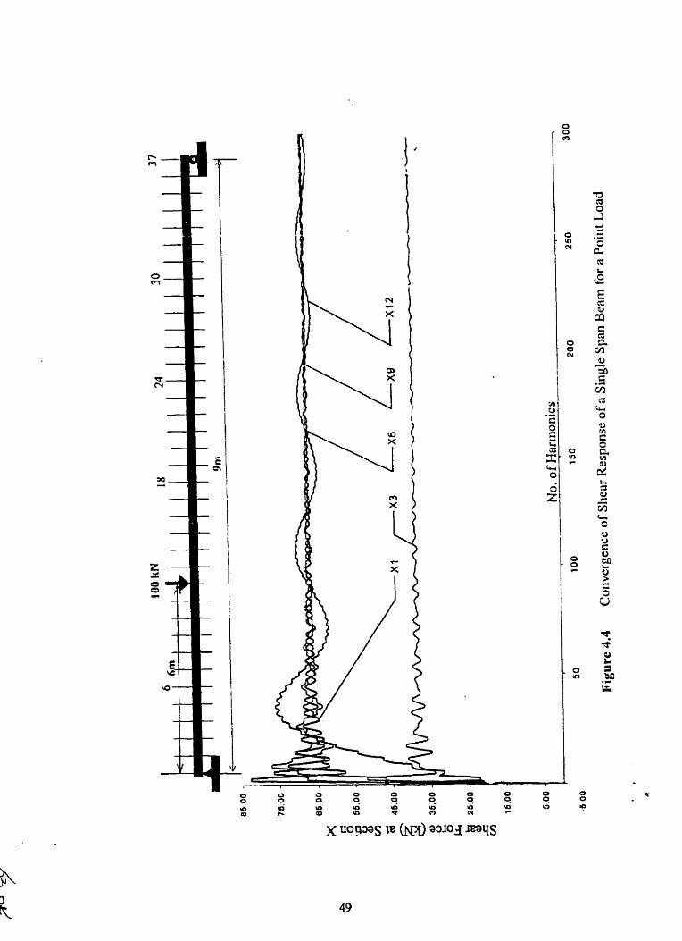
To study the convergence of shears at various sections, six sections Xi (lefi suppori), X3,
Xs, X9, Xiz, and Xi3 (under the load) were selected. Each section is 0.25m apart (as the
beam is divided into 36 equai sections). The convergence of shear response at these
sections is illusûatëd in. F i w 4.4. It is noted that in this and the subsequent figures, the
plots start fkom haxmonic zero. The values at zero harmonics should be disregarded as
being fictitious. Following conclusions are drawn fiom this figure.
1. Shear converges at a very slow rate at section XI2, close to load position.
2. Shear convergence at the support at section Xi, is the fastest.
For the same beam, the moment response is obtained and plotted in Figure 4.5, for n = 1,
3, 7, 12, 18, 27, 40, and 70. It can be seen h m this figure that the convergence of

601 Figure 4.2(b) Eff'cts of Higher Harmonies on Shear Response

2PL " 1 nnc nnx MW, = -- &sin-sin- n2 .=, n- L L
""i '-140
-1 60
Fi y r e 4.2(c) Effects of Higher Harmonies on Moment Re~onse
46
Rints a k q span
Figure 4.2(d) EEects of Higher Harrnonics on Deflection Reqonse .r -
47

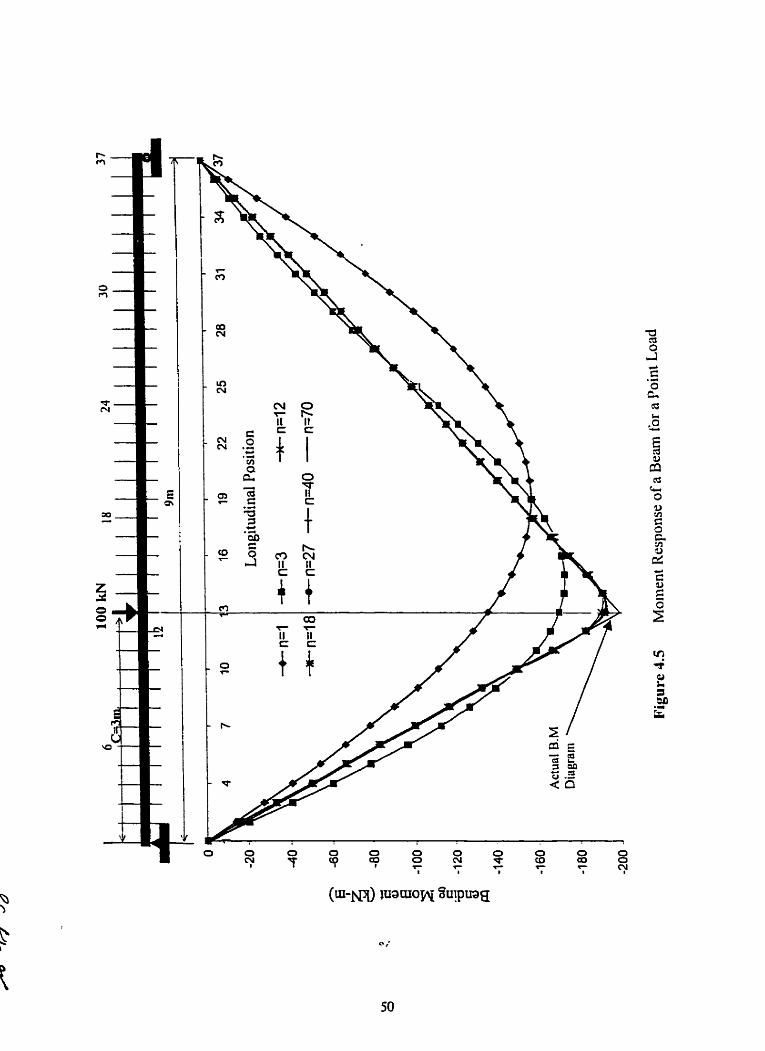

moments is much faster than that of shear. It can be seen that after about 18 hannonics,
the bending moment diagram obtained by harmonic analysis becomes fairly close to the
actual bending moment diagram.
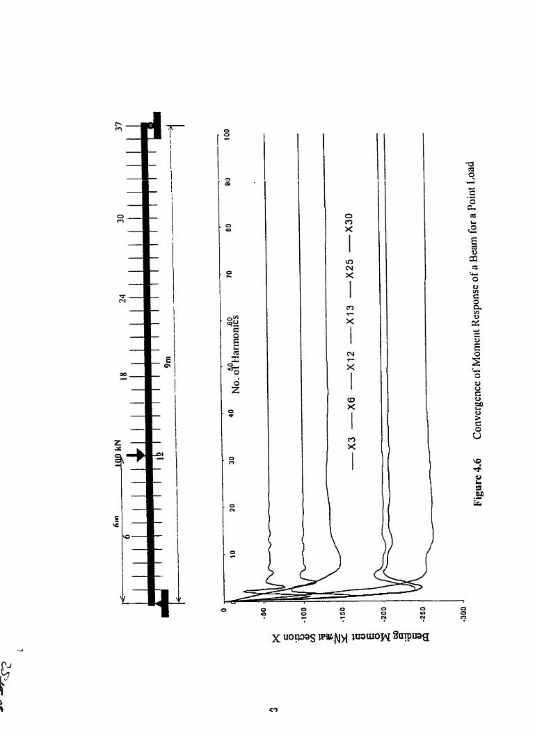
The convergence of moment results at sections X3, Gy XIZi XII, XU, and are plotted
in Figure 4.6. A clear trend does not seem to emerge fkom these plots, other than the fact
that moments away nom the load converge somewhat slower than those under the load.
42.2 Response uoder multiple loads
A simply supported beam of span 27m was loaded with one line of wheels of the
OHBDC truck positioned for maximum bending moment effects. The equivalent
hannonic representation of the truck loading is shown in Figure 4.7. In this and
subsequent figures dso, the beam length is divided into 36 equal parts leading to 37
reference points.
Although the magnitude of px itself does not have a direct influence on load effects, it is
instructive to see that after 40 harmonics, the distributed loads are still not closer to the
actual loads. The shear response of the beam under truck loading placed differently is
shown in Figure 4.8. As compared with single load, the shear convergence for truck
loading is quite fast. It took only 18 harmonics to achieve the same degree of
convergence as was obtained for the single load after 40 harmonics.


The shear convergence trends at sections Xi, Xi, &, X,, XI*, and Xi5 are plotted in
Figure 4.9. Following conclusions can be drawn from this Figure.
1. The convergence of shear response at all sections under multiple loads is
much faster than for single loads.
2. At section X3, being close to a support, the convergence is reiativeiy fast.
3. At sections &, X7, and Xi5, in close vicinity of loads, the convergence is slow.
4. At left support, the convergence is relatively faster than those at sections X3,
X7, Xis.
The moment response for the beam under truck loading is shown in Figure 4.10. Again,
as compared with single-load case. where 18 harmonics yielded virtually complete
convergence, oniy 1 2 harmonics produced v h a l l y complete convergence.
Moment convergence at sections Xi, X3, X6, X l t , and Xi5 is illustrated in Figure 4.1 1.
This figure aiso supports the conclusions dnwn fiom sheilr convergence results Le.,
convergence at sections &, X7, Xis, in the vicinity of the load, is slower than at X3,
which is farther away fkom loads.
4 2 3 Effect of load spacing
A simply supported beam of span 36m was loaded with 7 loads of equal magnitudes and
equally spaced. Three spacings were used in the analysis, being lm, 3m, and 5m.


Convergence of shears and moments were studied at various sections for each case
separately.
Shears at sections XI, X3, X s, Xi , X12, XI6, X19 were obtained and are plotted in
Figure 4.12, 4.13, and 4.14 for spaclig of lm, 3m, and Sm, respectively.
Following conclusions are drawn:
1. At section X5, the convergence for S = 5m is slower than for S= 3m.
Note that for S = lm, Xs represents section under the load and hence
should not be compared with S = 3m and Sm cases.
2. At section X7, the convergence is faster for S = l m than for S = 3m.
Again, the section X7 for S = Sm represents a different load condition
(away kom load) and therefore is not compared with spacing cases 1
and 2.
3. At section XIo (for S =3m and 5m) convergence is faster for closely
spaced loads.
Convergence of moment results at sections X6, X12, Xl5, XII, Xis and Xi9 is illustrated in
Figures 4.15, 4.16, and 4.17 for load spacing of lm, 3m, and 5rn respectively. Following
concIusions are drawn:
1. At mid-span (Xis), the moment converges virtually completely at n =10 for
lm spacing and whereas it took 30 harmonies for 3m spacing.


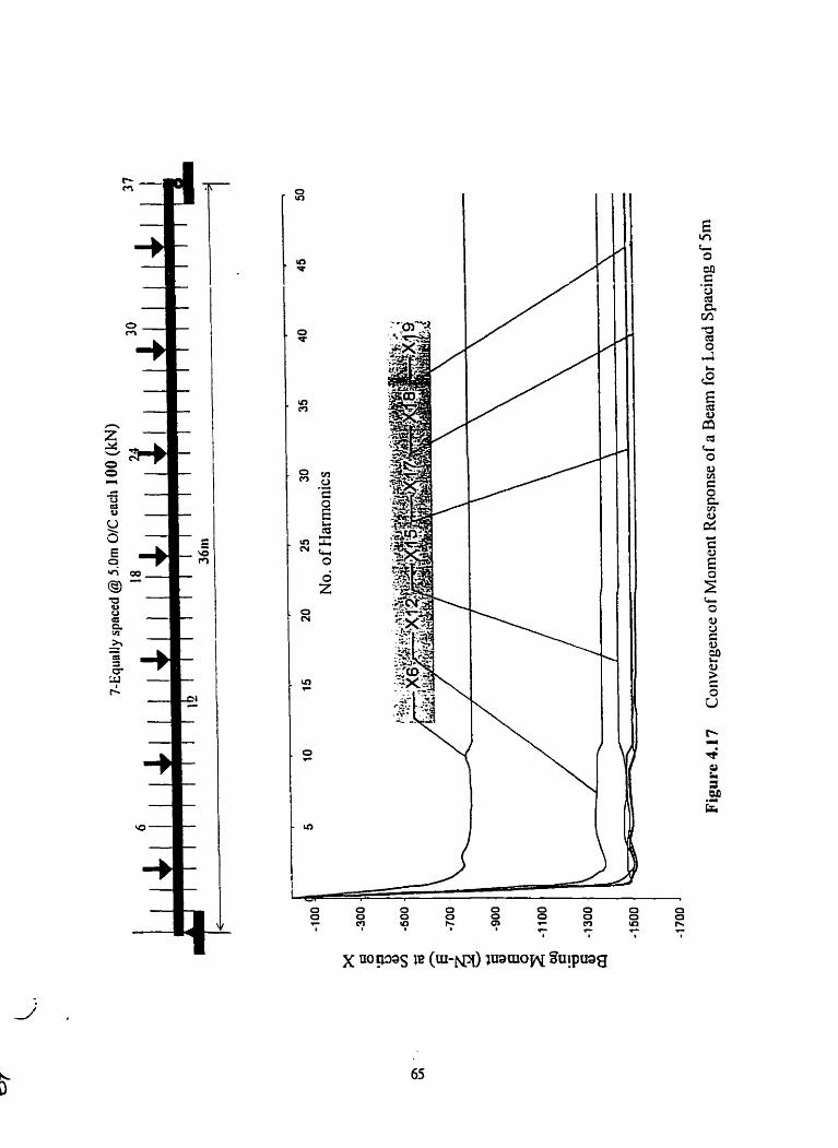

2. At section Xia, it takes 1 5 harmonics for 3m spacing and 22 harmonics for Sm
spacing to achieve nearly full convergence of moments.
3. The general trend of moment convergence shows slower convergence for
widely spaced loads and vice versa
43.4 Response of a continuous beam under multiple loads
A three span beam with the middle span of 16m and side spans of 10 m each was loaded
with the OKBDC truck with first load of 30 I<N positioned at the center of the first span.
F i r s ~ the intemediate reactions of the beam were calculaied as follows:
1. Intermediatr supports were removed and deflections computed at support
locations as: Ai = 2.285~1 O'/EI and A2 = 2 . 0 9 8 ~ IO'/EI.
2. The unit load was apptied at support locations and deflections computed as:
tjl = Szz = 6.26xidE1 and hi = 6 i2 = 5.07x10~1~1. It is recalled hat the 1"
subscript corresponds to the point, at which deflection is k i n g computed,
whereas the 2" subscript represents point where unit load is being applied.
3. Support reacùons RI and R2 were computed as shown below.
This gives, Ri = 272.3 kN and R2 = 114.5 W. These reactions were üeated as negative
loads acting at 10rn and 26m distances fiom the lef? support. Using spreadsheet program
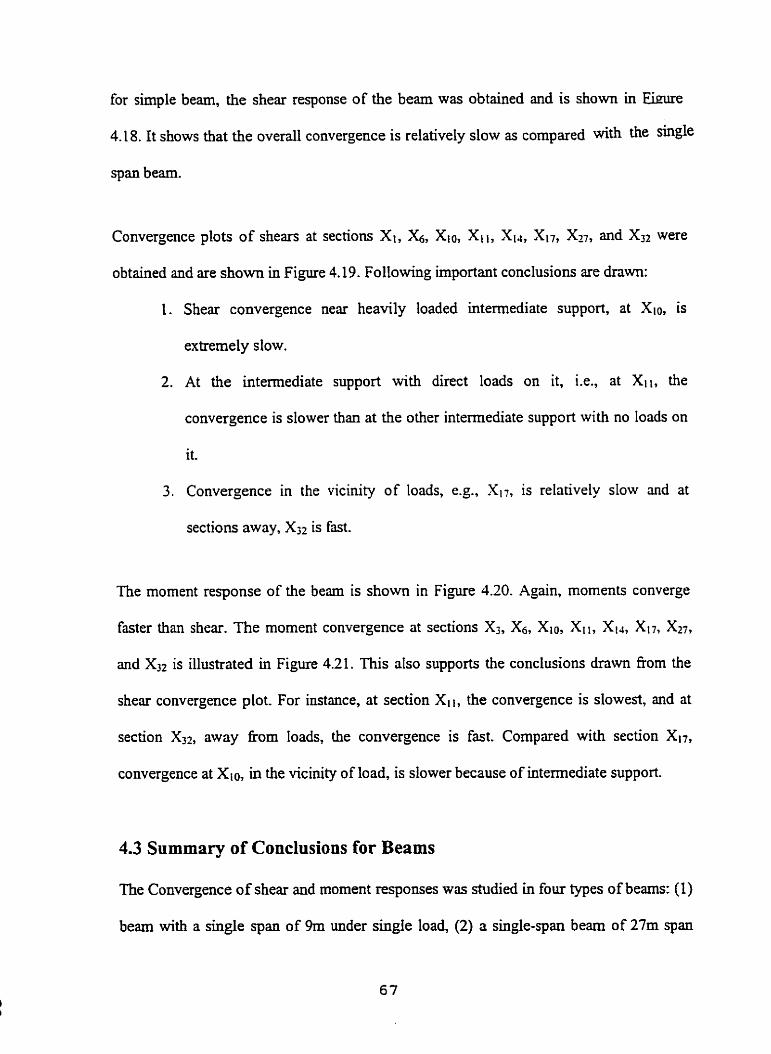
for simple beam, the shear response of the beam was obtained and is shown in Eiwe
4.18. It shows that the overall convergence is relatively slow as cornpareci with the single
span beam.
Convergence plots of shem at sections Xi, &, XIO, XI 1, XI J, &, X27, and X32 were
obtained and are shown in Figure 4.19. Following important conclusions are drawn:
1. Shear convergence near heavily loaded intermediate support, at Xia, is
extremely slow.
2. At the intermediate support with direct loads on it, i.e., at Xi , , the
convergence is slower than at the other intemediate support with no loads on
it.
3. Convergence in the vicinity of loads, e.g., XI7, is relatively slow and at
sections away, Xj2 is fiut.
The moment response of the beam is shown in Fi~ure 4.20. Again, moments converge
faster than shear. me moment convergence at sections X3, X6, Xlo7 XII , &J, X17, XZl ,
and XJt is illustrated in Figure 4.21. This also supports the conclusions drawn fiom the
shev convergence plot. For instance, at section XI,, the convergence is slowest, and at
section X3?, away fkom loads, the convergence is fast. Compared with section XI7,
convergence at XIo, in the vicinity of load, is slower because of intemediate support.
4.3 Summary of Conclusions for Beams
The Convergence of shear and moment responses was studied in four Srpes of beams: (1)
beam with a single span of 9m under single Ioad, (2) a single-span beam of 27m span


under OHBDC truck load, (3) a single span of 36m span with six loads of equal
magnitude and different spacing, and (4) a three span beam with a central span of 16m
and outer spans of 10m each. In each beam, the total length of the beam was divided into
36 equally spaced sections, Le., a total of 37 sections (XI through X3,). Convergence of
shear and moment responses was then obtained at the selected sections, in most cases, for
up to 300 harmonics. The summary of these results is shown in Table 4.1.
Table 4.1 No. of harmonics required for 990/6convergence in beams
1 1 No. of harmonies for 1 No. of harmonies for
Beam Case max. Moments
Sections 1 Other mas. Shears
Sections 1 Other
SS beam with single load
SS beam with OHDBC Ioad
4.4 Convergence of Responses in Girder-Slab Bridges
near loads 90-100
3-span beam with OHDBC load
4.4.1 Response Under Single Load
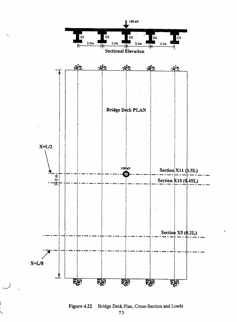
Consider a single span bridge of span 30m with a single point load of 100kN acting at
mid span as shown in Figure 4.22. The bridge has five girders, each with a uniform
moment of inertia of 2-39 m4, torsional inertia of 0.0254 m4, and a d o m sIab thickness
of 0.24m. Using spreadsheet programs of semi-continuum method discussed in chapter
30 - 40
secrions 35-70
J O - 200
1 I
near loads > 300
20 - 30
sections 45 - 300
90 - 300 15 -20 > 300 I
>450 110-300
Sectionai EIevation
Bridge Di
Figure 4.22 Bridge Deck Plan, Cross-Section and Loads 73
three, the response of bridge was computed in longitudinal direction and the convergence
of results studied at various sections of the bridge, which are aiso identified in Figure
4.22.
4.4.1.1 Longitudinal Shear in Girders
For the Ioading shown in Figure 4.22, longitudinal shear in various girders was obtained
and plotted in Figure 4-23. It can be seen that the middle girder (G3) carries the major
share of longitudinal shear. Only a midl Eaction of the total longitudinal shear is
transferred to the outer girden G1 and CS.
The iongihidinal shear of girders G1 and G3 was obtained for hamionics it = 1 , 3, 7, 12,
18, 27.40, and 70 and is plotted against the span in Figure 4.24. The 30m span is divided
into 20 equal sections of 1.5 length. Figure 4.24 shows that convergence of shear in
grder G1 is very fast and only afier 12 harmonics Wtually complete convergence is
attained. The convergence of shear in the directly loaded girder G3 is, however, very
slow and even d e r 40 hmonics the shear is not hlly converged.
The convergence of longitudinal shear in girders G1 and G3 was studied at two cross-
sections Xs and Xio, as identified in Figure 4.22. The results are shom in Figure 4.25. It
can be seen that the shear convergence in girder G1 is quite fast wbereas in girder G3 it
almost took 50 harmonics for X5 and over 300 harmonics for XI2, which lies in close
vicinity of the point load.


Figure4$#Longitudmal Girder-Shear D&'bution (Typical Slab-Girder Bridge)

Convergence o f Shear in Girder G1
O No. of Warmonics I r 1
50 100 1 50 200 250 300
Convergence of Shear in Girder G3
Figure425 Convergence of Longitudinal Girder Shear (Typical Slab-Girder Bridge)

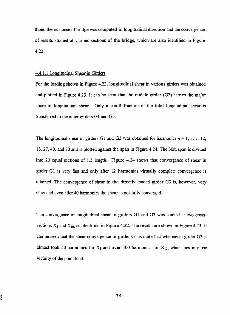
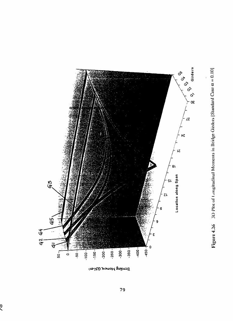
1.4.1 -2 Longitudinal Moment in Girders
Longitudinal moments in the girden under the central point load are shown in Figure
4.26. Again, the central @der canies the main share of total longitudinal moment. The
moment response of girders G1 and G3 for n = 1, 3, 7, 12, 18, 27, 40, and 70 was
obtained and plotted in Fi-ure 4.27. The moment convergence in girder G3 i s very slow
as compared with girder G 1 .
Moment convergence in girders G1 and G3 at sections Xs and Xi 1, identified in Figure
4.22, is illustrated in Figure 4.28. It can be seen in this figure that while the moments
virtually converge at n = 3 for girder G1, the moments in &der G3 are slow to converge
and for section Xi ,. It took 46 hmonics to achieve 99.9% convergence.
44.2 Respoase Under OHBDC Truck Loads
The typical girder-siab bridge was loaded with the OHBDC truck positioned to produce
maximum bending longitudinal moments; the truck location is shown in Figure 4.29. The
longitudinal responses of the bridge were obtained and are discussed in the following
sections. The convergence of results is also compared with single load responses
discussed in section 4.3.1.
4.4.2.1 Longitudinal Girder Shean
The longitudinal shear response of the bndge under the truck load is shown in Figure
4.30. Convergence of longitudinal shear results in girders G1, G2, and G3 at sections &,
Xj, Xs, Xioms, and Xis are shown in Figure 4.3 1. It is observeci that the convergence of

Longitudinal S hear in Girder G3
Figure427 Lonpitudkl Girder Moment Distn'bution .
(Typicd S lab-Girder Bridge)

C o n v e r g e n c e of M o m e n t s in Gi rder G l
XI1
N o . o fhar rnon ics I I r 1
C o n v e r g e n c e of M o m e n t in G i r d e r G 3
O , No. o f harmonics I t
Figure4.3 Convergence of LongÎtudinal Guder Moments (Typical Slab-Girder Bridge)

Sectional Elevation
?$j$ :$& & ! 1
1 l 1 . 1 I
~igure4i2(1 Bridge Geomeûy and Load Codiguration
82

F i p m 4 3 0 Distniution of Longitudinal Shear

4 '1 1
Girders 1 & 5
~ 1 6 . 5 Xi5 2 -.
No. of Harmonies 0 , - I
1 6 11 16 2t 26 31 36 41 46
\ \ - - - X10.5 X l 5
No. of Hamonics
Convergence of Longitudinal Shear in Girders

results is very slow in the externally loaded girder G3 and quite fast in extemal girder G1.
Convergence is aiso slow in girder G2, also extemally loaded. It is interesting to note that
the longitudinal shear in G3 is not fully converged even dter 400 harmonics. The results
in G 1 are however virtuaîly converged within 5 harmonics.
Compared with the smgle load, the overall convergence is relatively ht. For instance, in
Gl it takes only 3 harmonics to achieve virtuaily Full convergence as compared with 7
harmonics in case of single load.
4.4.2.2 Longitudinal Girder Moments
The longitudinal moment response of the bridge under the OHBDC truck is s h o w in
Figure 4.32. The convergence of results for girdes G1, G2, and G3 for sections X3, Xo.
Xg, XI2, and Xis is shown in Figure 4.33. Moment convergence is relatively fast
compared with shear convergence.
Compared with the single load case, the overail convergence is again relatively Fast. For
instance, in G3 it takes ody 20 harmonics to achieve virtually full convergence as
compared with 50 hannonics in case of a single load.
4.5 Convergence of Results in Torsionally Soft Girder Bridges
The convergence of responses in a torsionally sofk bndge was studied by using the lowest
value of the characterizing parameter a, Le., 0.06, as described in chapter two. Using a
value of 0.06, values of 1 and J were obtained as 3.32m4 and 0.018rn4 respectively.

OHBDC Truck
~ i ~ u r e 4 3 2 Distribution of Longitudinal Moments in Girdes

No. of Harrnonks
ex9
Girders 1 & 5
M. d Hamm- I
Gitdet 3 X3 X6 X 9
Figurd33Convergence of Longitudinal Moments in Girders
87

The response of the bridge under a single point load of 100 kN load was then obtained in
longitudinal direction. The results were also compared with the typical bridge case
studied in section 4.4.
45.1 Longitudinal Shears in Girden .
For the truck loading shown in Figure 4.22, the longitudinal shear response of the bridge
was obtained and plotted in Figure 4.34. The longitudinal shear distribution in &der G3
resembles the shear distriibution correspondhg to a uniformiy distributed Ioad. The
difference in shears for n = 1 and n= 3 was found to be much smaller in tosionaily soft
bridge than it was in case of the standard bridge exarnplë. For the extemally loaded
@rders, the lower value o f a had, however, little erect on the overall shear distribution.
The convergence of longitudinal shears in girden Gt and G3 is ploned in Figure 4.35 and
shows that the convergence is in the torsiondly soft bridge is better only in girder G1
which is not extemally loaded.
45.2 Longitudinal Moments in Girders
1
The longitudinal moment response and the convergence of moment results are shown in
Figures 4.36 and 4.37 respectively. Conclusions drawn fkom shear response were also
found valid for the moment response. The convergence in extemal girder G1 was sfightly
impruved due to a lower value of a. The convergence of results was however not afTected
in extemally loaded girders G2, G3, and G4.
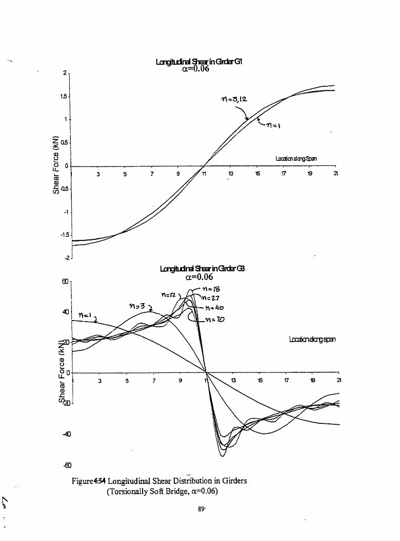
2,
15 -
1
su- - al t) 0 O - U, L m
;a-
-1 .
-1.5 -
-2 J
Figure- Loetudinal Shear ~istnbution in Gkders (Tonionally So fi Bridge, a4.06)

Convergence of Shear in Girder G1 u=0.06
O No, of Harnunics
1
25 50 75 100 125 150 175 2ûû î2S 250 275 300
Convergence of Shear in Girder G3 a=0.06
x5
i
No. of Hamonics
Figure4i35 Convergence of Longitudinal Shear Distribution in Girden- (Torsionally Soft Bridge, a4.06)
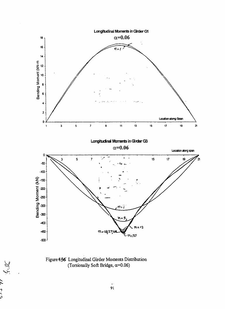
Figure 436 Longitudinal Girder Moments Distribution (Tonionaliy Soft Bridge, a=û.06)

Convergence of Longiiudianl moments in 01 a=OaO6
No. of harmonies 1 I I i 6 1 1 1 I 1
Convergence of longitudinal moments in girder G3 ~=0.06 NO. of hamonics
1 1 1
15 ' a) 25 30 35 40 45 50
-100 -
Q)
5 -250 - 2 0 300 - t - u C -350 - Q) m
400 -
450 -
Figure437 Convergence of Longitudinal Girder Moments (Tosionally So ft Bridge, a=0.06)
4.6 Convergence of Results in Torsionally Stiff Girder Bridges
The convergence response of a torsionally stiff bndge was obtained by using the highest
practical value of the characterizhg parameter a, being 0.20, as descnbed earlier. Using
a value of 0.20, trail values of 1 and J were found as 1.45 m4 and 0.045m4 respectively.
The response of the bridge under single point load of 100 kN load was t ' en obtained in
longitudinal direction. The results were also compared with the typical bridge case
studied in section 4.3 and the torsionally soft bndge discussed in section 4.4.
46.1 Longitudinal Shear in Girders
For the truck loading shown in Figure 4.22, the longitudinal shear response of the bridge
was obtained and plotted in Figure 4.53. Since al1 girders are tonionally stiff or f i e d l y
sofi, the outer &der G1 has more uniform distribution of longitudinal shear. Also, the
girders Gl and G3 have the same +ve sign for the longitudinal shear, which was the
opposite in previous cases of standard and torsionally soft bndge examples.
The convergence of longitudinal shears in girder G1 and G3 is plotted in Figure 4.54 and
shows that the convergence is also improved in tonionally stiff bridge but oniy in &der
G1.

z-a, x
Figure33 Longitudinal Shek Distriiution in Girders (TorsionalIy Stiff Bridge, a=0.20)

Convergence of Shear in Girder G l cl=0.20
Convergence of Shear in Girder G3 a4.20
1 -
-1
No. of Harmonics . - . .
i I 1 1
O EO 100 150 2CO 250 3CO
0.4 - 0.2
FigurekW Convergence of Longitudinal Shear Distribution in Girders (Tosionally Stiff Bridge, a=û.20)
-L No. of Harmonics

4.6.2 Longitudinal Moment in Girden
The longitudinal moment response and the convergence of moment results are shown in
Figures 4.40 and 4.41 respectively. Conclusions drawn from shear response were also
found vdid for the moment response. The convergence in extemal girder G1 was slightly
irnproved due to a higher value of a. The convergence of results was however not
affected in extemally loaded girden G2, G3, and G4.
4.7 Summary of Conclusions for Bridges
Convergence of shear and moment responses was siudied in four types of bridges: (1)
standard bndge with a single span of 30m under single load, (2) a single-van standard
bridge of 3lhn under OHBDC tnick load, (3) a single-span torsionally-stiff bridge of 30m
span with OHBDC truck load, and (4) a single-span torçionally-soft bridge of 3 h span
with OHBDC tnick load. The summary of these results is s h o w in Table 4.2.
Table 4.2 No. of harmonies required for 99% convergence in bridges
Longitudinal Response of Girden
Bridge Case Eiienzally looded g irders
Girders not cav'ng the load
directly
Standard bndge with single load Standard bridge with OHDBC load Torsionall-stiff bridge with OHDBC Ioad
M.
46
42
Torsionally-Soft bridge with O m B C load
Mx
3
v x
>400
46
v x 7
1 r
3 >400 2
6 >400
6 42
2
>400 2

~i-gue Longitudinal Girder Moments Distriiution (Ionionally S t E Bridge, a=0.20)

Convergence of Longitudianla moments in Gl a*.20 No. of hannonics
Convergence of longitudinal moments in girder G3 a=k2 0 No. of hamonics
~igure&i?& Convergence of Longitudinal Girder Moments (Tonionally Stiff Bridge, a=0.20)

The foilowing conclusions are drawn fiom the snidy:
In case of beams:
1. The convergence of moments is faster than that for shears.
2. The convergence near load and support locations is slower than at other
locations.
3. The convergence in beams with closely spaced loads is faster as compared to
those with widely spaced loads.
In case of bridges:
1. The convergence of longitudinal shean is slower than that of longitudinal
moments.
2. The convergence of longitudinal responses in extemally loaded girders is
s Iow.
3. The overail convergence of various bridge responses is fast in the case of
truck loading as compared to single load case.
4. For torsionally soft and sûff bridges, convergence of longitudinal moments in
rmemally loaded girdes is slightiy improved.

Chapter 5 Hastening Convergence
Of the Orthotropic Plate Solutions
The onhotropic plate method For rectangular plates supported on two opposite edges
(Cusens and Pama, 1975) is based on a series solution. The convergence of this method is
slow especially for h e m . As many as 50 harmonics may be required to achieve vinually
complete convergence. The orthotropic plate method is currently being incorporated in a
program, called PLATO.
The semi-contjnuum method of analysis (Jaeger and Bakht. 1989j, incorporatecl in a
program called SECAN, is also based on a senes solution. However, the use of a novel
technique has ensured rhat its results converge very quickly. Only five harmonics are
aften sufficient to obtain virtually cornpkte convergence even for longitudinal shean.
The purpose of the current project is to demonstrate numerically that the technique of
hastening convergence employed in the semi-continuum method cm also be applied to
the orthotropic plate method.

5.2 Lllustration of Convergence Technique in the Semi-continuum Method
To illustrate the technique of quick convergence used in the semi-continuum method, a
five-girder bridge, described earlier in chapter 4, is considered with a central load of
100kN; this bridge has a simply supported span of 30m. and its various other properties
are noted in section 4.4.1.
Figure S.l(a) shows the triangular kee moment diagram for the centrai girder, which
carries the applied load directly. It is recalled that the free moment diagram for a directly
loaded girder represents the bending moments that the girder would have sustained in
isolation from the other girden. The fiee shear and deflection diagrams are obtained
similady. The maximum free bending moment = 4 x 100 x 30 / 4 = 750 W.m.
In the serni-continuum method, quick convergence of bending moments is achieved by
subtracting f5orn the fÎee bending moment diagram those bending moments which are
passed on to the girders not d i d y carrying the appiied load.
As shown, for example by Jaeger and Bakht (1989), the bending moment Adx dong the
beam due to a central point load P on a simply supported beam of span L is given by
equation 2.4.

Figure 5.1 Bending Moments: (a) Free Bending Moment Diagram; (b) Bending Moment Diagram due to First Harmonic
The first harmonic moment given by the moment equation, for n =1 is illustrated in
Figure j.l(b). The maximum bending moment at the mid-span is found to be 607.92 W.
as dso shown in this figure.
Jaeger and Bakht (1989) have given expressions for distribution coefficients for
distributing load effects in 5-girder bridges. It is noted that these coefficients. meant for
manual cdculations, do not give as accurate results as the computer prognm. For a load
at the middle girder, the distribution coefficients for the five girders of the bridge under
consideration the first harmonic are found to be -0.009, 0.262, 0.494, 0.262, -0.009,
respectively. These coefficients imply that for the first harmonic. 49.4% of the bending
moments shown in Figure j.l(b) are retained by the rniddle girder, and a total 50.6% are
passed on to the remaining four gîrders. The former moment diagram is presented in
Figure 5.2(a), and the latter in Figure 5.2@). As shown in Figure 5.2(b), the maximum

bending moment passed on to the four girders after considering only the fïrst harmonic is
the sum = 0.506 x 607.92 = 307.61 kN.m.
As will be shown later, the k t harmonic bending moments for the middiz girder are
significantly different nom the 'fuily-converged' moments, which can be obtained
inefficiently by adding the distributed effects for higher harmonics. In this process, for
each successive hannonic, the intensity of the mêuimurn Adr goes on reducing because of
nL in the denorninator of the & equation, and the value of the distribution coefficient
goes on increasing for the directly-loaded girder. For example, the values of its
coefficiènt for 2nd, 3". 4", and 5' harmonics are 0.82, 0.94, 0.98, and 0.99, respectively.
For the stmcture under consideration, the process of adding the effects of the various
harmonics to achieve about 98% convergence required the considention 01 20 harmonics.
After 350 harmonics, the mid-span moment in the middle &der was 437.34 W.m. While
the process of addition kept changing the moments in the middle girder with every
harmonic, the moments in the outer four girders did not change afier the 5' harmonic.
The fact that the distribution coefficient for the srn harmonic for the directly-loaded girder
is 0.99 indicates that for the 5' and higher harmonics, only 0.01 % of the moments given
by the Mx equation are passed on to the remaining four girders. As explained in the

following, advantage c m be taken of this property of distribution to hasten of load effects
in the directly-loaded girder.
(cl
Figure 5.2 Bending Moment due to k t Hannonic: (a) Moments Retained by the
Middle Girder; (b) Moments Passed on to Outer Four Girders; and (c)
Moments Passed on to Outer Four Girders Deducted from the Free
Moment Diagram
Instead of adding the distnïbuted moments for the loaded girder, one cm use the free
moment diagram (Figure 5.1 a), and start deducting the s u m of moments that are passed to
the girden not carrying the applied load directly. The mid-span £iee bending moment is

750 kNm, and the mid-span moment passed on to the outer four girders for the first
hamionic = 307.61 kN.m. Hence, the mid-span moment in the middle girder after
considering only the first harmonic = 750.00 - 307.61 = 442.39 kN.m; this process is
illustrated in Figure 5.2 (c) . After considering only £ive harmonies, the value of this
moment is found to be 438.22 kN.m. which is within 0.2% of rhe value obtained by
considering 350 h m o n i c s in the process of adding the load effects for the loaded girder.
Figure 5.3 contains hvo sets of plots of mid-span girder moments obtained by the manuai
method by considenng only the first harmonic. In one se t al1 the girder moments were
obtained by multiplying the moments given by &lx equation with the relevant distribution
coefficients. In the second set, moments in the outer girders were obtained by the same
process as used for the first set; however, the moment for the middle girder were obtained
by using the process illustrated in Figure 5.2(c).
The bridge under considention was also analyzed by SECAN. The mid-span moments
were found to have converged virtually completely after 5" harmonic. The SECAN
bending moments correspondhg to 5 hamonics are also plotted in Figure 5.3. It c m be
seen that these results, representing nearly MIy converged moments, compare very well
with those obtained by the manual method, incorporating the quick convergence scherne.

I , W = 12.5 m
< i Actual Slab-Girder Bridge ;
d
Figure 53 Cornparison of Mid-Span Girder Moments Obtained by the Manuai and
Computer-Based Semi-Continuum Methods
5.3 Convergence of Results in Orthotropic Plate Method for Girder
Bridges
In order to illustrate the hastening technique in girder bridges three cases are studied,
these being, (1) a single span girder bridge under single central-load, (2) a single span
&der bridge %?ch OHBDC û-iick Ioad, and (3) a Pxo span &der bridge under OHBDC
truck loading.
53.1 Single Span Girder Bridge with Single Lord
A single span girder bridge of span and width as s h o w in Figure 5.4 with a centrai load
of 100 kN was anaiyzed using PLATO. The expressions for obtaining the plate rigidities
are as
given in the Ontario H i w a y Bridge Design Code (1992); these expressions are also
given in various text books (e.g., Bakht and Jaeger, 1985). The program PLAT0 handles
rectmgular patch ioads. As s h o w in Figure 5.4, the central patch load of 100 kN was
represented as a 0.25 x 0.60 m patch load, with the former dimension being in the
longitudinal direction of the bridge. Also as shown in this figure, the x and y axes of the
plate are dong the longitudinal and transverse directions, respectively. Various
parameten of this girder bridge and the related plate rigidities are summarized below.

Table P l Girder bridge properties
Y
and torsional rigidities dl
12.5 m
0.24 m
Q)
E O
8
L L Q) a bl". Z:
1 D.,=/ 1.016E5kN.m 1 Transverse Flexurai and
-
Width (W) =
Slab thickness (t) =
G = 1 1E7kN/m2 Poisson's ratio u = I O
Coupling rigidities
Y Figure 5.4 Single Span Girder Bridge [Single Load]

5.3.1.1 Convergence of Longitudinal Moments
The girder bndge idealized as equivalent orthotropic plate was analyzed for mid-span
longitudinal moments. PLAT0 results for 1 M , were obtained for various hamonics at 11
equidistant points and are shown in Table 5.1 for different number of harmonics. The
longitudinal moment inteosities My at the mid-span are plotted for n = 1 and 50 in Figure
5.5 which also indicates the transverse positions of the girders on the ideaiized plate. In
order to obtain the corresponding moments in a girder from this figure, one has to
integnte the area under the relevant curve over the width that represents the girder. It was
found that for I and 50 hmonics. the areas of the corresponding curves over the width
represented by the middle girder are 276.71 and 432.3 1 I<N.m, respectively. It can be seen
in Figure 5.5 that the 50-n curve is different fiom the 1-n curve mainly within die width
represented the directly-loaded, i.e., the middle girder. By taking a cue from this
observation, the convergence technique of the semi-continuum method is tried as follows.
The shaded area in Figure 5.6, representing the moments passed ont0 the four outer
girders is found to be 33 1.78 kN.m for n = 1. The mid-span moment retained by the
middle girder is, therefore, = 746.88 - 33 1.78 = 4 15.1 kN.m. It can be seen that this value
is fairly close to that obtained for 50 harmonics.

Actual Slab-Girder Bridge
Equivalent Ortho-plate Rigidities 0.60 m D,= 191.ZE5 W.m, Dy=0.23E5 ~mb-4
i / D, = 1 .OZES kN.m, & = 0.23E5 kNm
D,=D2=0 i-,
Equivnlent Orthobopic Plate
Externail y Loaded Girder
Tranverse Loac tion
Figure 5.5 Transverse Distribution of Longitudinal Moment in Girder Bridge [Single Span & Single Load]


Table 5.1 Vaiues of 1% obtained bv PLAT0 at x = 1 5 m, in kN.mlrn
The above examples have shown that the technique for hastening convergence can be also
employed gainhlly in conjunction with the orthotropic plate method for converging
longitudinal moments in girder bridges. Ln using this technique, the moments passed on
to the girders not carrying the Load directly are obtained by discounting the width of
- .-
orthotropic plate representing the directly-loaded girder. It is shown in Appendix E that
the process of hastening convergence is relatively insensitive to the width of the load.
5.3.1.2 Convergence of Lon~itudinal Shears
The idealized isotmpic plate discussed earlier was also anaiyzed for longitudinal shears
due to various number of harmonies at x = O using PLATO. The resdts are shown in
Table 5.2 and plotted in Figure 5.7. Convergence of shears in extemally loaded girder
(ELG) is extremely slow.
n.15
-20.3 2.7
n=sO
-20.3 2.7
n=350
-20.3 2.7
1
-20.3 2.7
Tmns. Points n i 5 n.7 / e 9 n=l
1 1 2
n=3
-20.3 2.7
-20.4 2.7
-20.3 2.7
-20.3 ] -20.3 2.7 1 2 . 7

'1
Actual Slab-Girder Bridge
Equivalent Ortho-plate Rigidities 0.60 m Dr= 191.ZE5 kN.m Dl.= 0.23E5 kN.m$
1 Dn*= 1 .O2E5 ~N. Ix I , D,= 0.23E5 k N - r n j m ~ IrN - - -
Equivalent Orthotropic Plate
Exremdly Loaded Girder
1
Figure 5.7 Transverse Distribution of Longitudinal Shear in Girder Bridge [Single Span & Single Load]

Table 5.2 Values of V' obtained bv PLAT0 at x = O, in W/rn
Longitudinal shears in ELG can be obtained as described earlier. The first harmonic
f i
shears passed on to outer slab are s h o w by hatched are in Figure 5.8. Longitudinal shear
(V') computations in the ELG are summarized below. V, in ELG using 50 harmonics,
Tmns- Points
represented by the area under V, curve was found to be 17.50 W.
n=9
Table 5.2.1 V' in ELG using Hastening Technique
1 2 3 4 5 6 7
n=l ni3 "=Il n=5
Total Free Shear
n.50 n=15 n=7
(VF) Shear in Outer Girders
n=350
-2.1 0.3 3.0 6.5
5OkN
(Vd Shear in ELG
The above table shows that the quick convergence scheme Ieads to more than 99%
-2.1 0.3 3.2
-2.7 0.3
-2.1 0.3 3.2 6.8
6.7 8 1 6.5
34.57
(&) % Accuracy
convergence of longitudinal shears d e r considering only 5 barmonics.
-2.1 0.3 3.2 6.7
-2.1 0.3 3.2
10.41 6.9
6.7 6.8
50kN
kN 15.86
-2.1 0.3 3.2 6.71
2 0.3
7.1 7.5
6.7 9 1 3.0.
12.6 ---- 10.4
50kN
33.75
kN 90.6 %
-2.1 0.3
6.7) 6.7
6.7 7.5
6.7 3.2,
1.7 6.9
32.96 kN
17.68
3.2 6.7 7.5 7.6
6.7
7.5
3.2.
10.8 7.6
3.21 3.2 6.71 6.7
6.7
kN 17.47
kN 98.9 %
7.6 7.5
3.2.
3.4 7.6
7.6
6.7
kN 99.8 %
3.21 3.21 3.2.
5.1 7.6
7.6
3.2.
9.5 7.5
3.2.
4.5 7.6


53.2 Single Span Girder Bridge with OHBDC Truck Load
The girder bridge described in section 5.3.1 was again andyzed for one line of wheels of
the OHBDC Tmck loading as s h o w in Figure 5.9. Loads were positioned to produce
maximum longitudinal moments.
Figure 5.9 Single Span Girder Bridge under One Line of OHBDC Truck Load ,
5.3.2.1 Convergence of Longitudinal Moments
PLAT0 results for longitudinal moments are shown in Table 5.3 and plotted in Figures
3-10 and 5.1 1. A cornparison of Figure 5.6 with 5.1 1 shows that the convergence of
longitudinal moments is relatively fast in this case of tnick load as compared to the single
load case.

One Line of WheeIs of OHBDC Truck
I'
Actual Slab-Girder Bridge
Equivalent Ortho-plate Rigidities n m m
One Line of Wheels of 0 I B D C Truck
*--
Equivalent Orthotropic Plate
Externatly Loaded Girder
375 ; I
275 1
Transverse
Figure 5-10 Transverse Distniution of Longitudinal Moment in Girder Bridge [Singe Span & Tmck Load]


Longitudinal moment (Mr) computations in the ELG using 50 harmonics and the
hastening technique are summarized below.
Table 5 3 Values of hlr obtained by PLAT0 at x = 15 m, in kN.m/m
LW'' in ELG using 50 harmonics, represented by the area under A& curve was found to be
816.72 W.m .
Table 5.3.1 Mx in ELG using Hastening Technique
1 No. of Harmonies
i ~ m s . 1 points I l
2
n=3
-61.0
,,=, -61.0 8.1
n=7
-61.0 8.1
The results given in above table show that the quick convergence scheme lads to more
than 99% convergence of longitudinal moments afler considering only 3 harmonics.
n=ll
-61.0
r0=5
-61.0
n=9
-61.0 8.1
Total Free Moment (MF)
Moment in Outer Girder (M. )
Moment in ELG ( M x )= - (Ma )
% Accuracy
3
n = 1 1806.8 lcN.m
993.03 mm 813.72 kN.m
99.6 %
n=lS
-61.0
88.3 88.2 8.1
88.3 ! 88.3 88.3 8.1
88.4 88.3 8.1
n=50
-61.0
88.3 1 88.3 8.1 i 8.1
~ 3 5 0
-61.0 8.1

5.3.2.2 Convergence of Longitudinal Shears
The idealized isotropic plate was analyzed for longitudinal shears at x = O using PLATO.
The results are shown in Table 6.4 and ploned in Figure 5.12. It cm be seen in these
figures that the convergence of shears in ELG is slower than that for corresponding
moments.
Table 5.4 Values of V, obtained bv PLAT0 at x = O. W/m
Longitudinal shears in ELG c m be obtained as described earlier. The first harmonic
-.
shears passed on to outer slab are s h o w by hatched are in Figure 5.1 3. The longitudinal
r~rans . Points
shear (V,) cornputations in the ELG are summarized below. Vr in ELG using 50
harmonies, represented by the area under V, curve was found to be 90.49 kN.
n =l
Table 5.4.1 Y, in ELG using Hastening Technique
n=3 1 n =5 I
Total Free Shear (Vd
Shear in Outer Girders N o
Shear in ELSS t
n=7
,
No. of Hamonics
1
n = I 200.15
kN 103.47
kN 96.68
n=15 / n=50 n=9 ni350 n=l4
n = 3 200.15
kN 1 10.22
kN 89.93
n = 5 200.15
kN 1
109.75 EcN
90.40
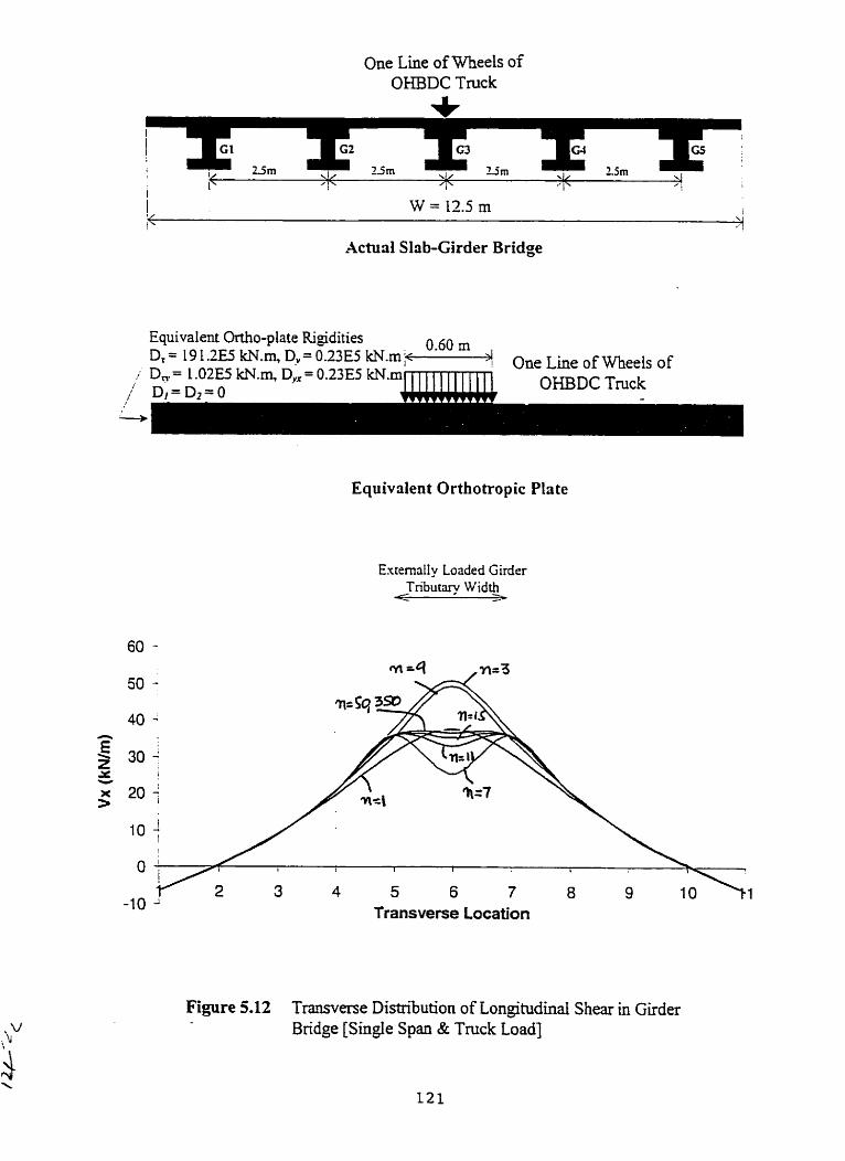
One Line of Wheels of OHBDC Truck
! - ;;
Actual Slrb-Girder Bridge
Equivaient Ortho-plate Rigidities 0.60 m D, = 19 1 JE5 kN.m D, = 0.23E5 kN.m $ >f One Line of Wheels of
i D , = L.02E5 kN.m, D, = 0.23ES kN.m D I = D 2 = 0 OKBDC Truck
Equivnlent Orthotropic Plate
Extemally Loaded Girder Tributam Width
Figure 5.12 Transverse Distribution of Longitudinal Shear in Girder Bridge [Single Span & Truck Load]


The above table shows that the quick convergence scheme leads to more than 99%
convergence of longitudinal shears after c o n s i d e ~ g only 5 harmonies.
533 Two Span Girder Bridge with OHBDC Truck Load
The 2-span girder bridge shown in Figure 5.14 was analyzed wing PLATO for
longitudinal moments and shears. The results are discussed in the following sections.
v
Figure 5.1 4 Two-Span Girder Bndge under One Line of OHBDC Truck Loûd
5-3 -3.1 Convergence of Lon&udinal Moments
PLATO results for longitudinal moments over the middle support are shown in Table 5.5
and plotted in Figures 5.1 5 and 5-16.

One Line of Wheels of OHBDC Truck
,
Actual Siab-Girder Bridge
Equivalent Ortho-plate Rigidities 0.60 rn D,= 19 1.2E5 kN.m, D,v= 0.23E5 kN.m b-4 One Line of Wheels of
OHBDC Truck - - - . - - - .- *--
Equivatent Orthotropic Plate
Externaily Loaded Girder
Y"' Transverse Location
Figure 5.15 Transverse Distribution of Longitudinal Moment in Girder Bridge [2-Span & Truck Load]
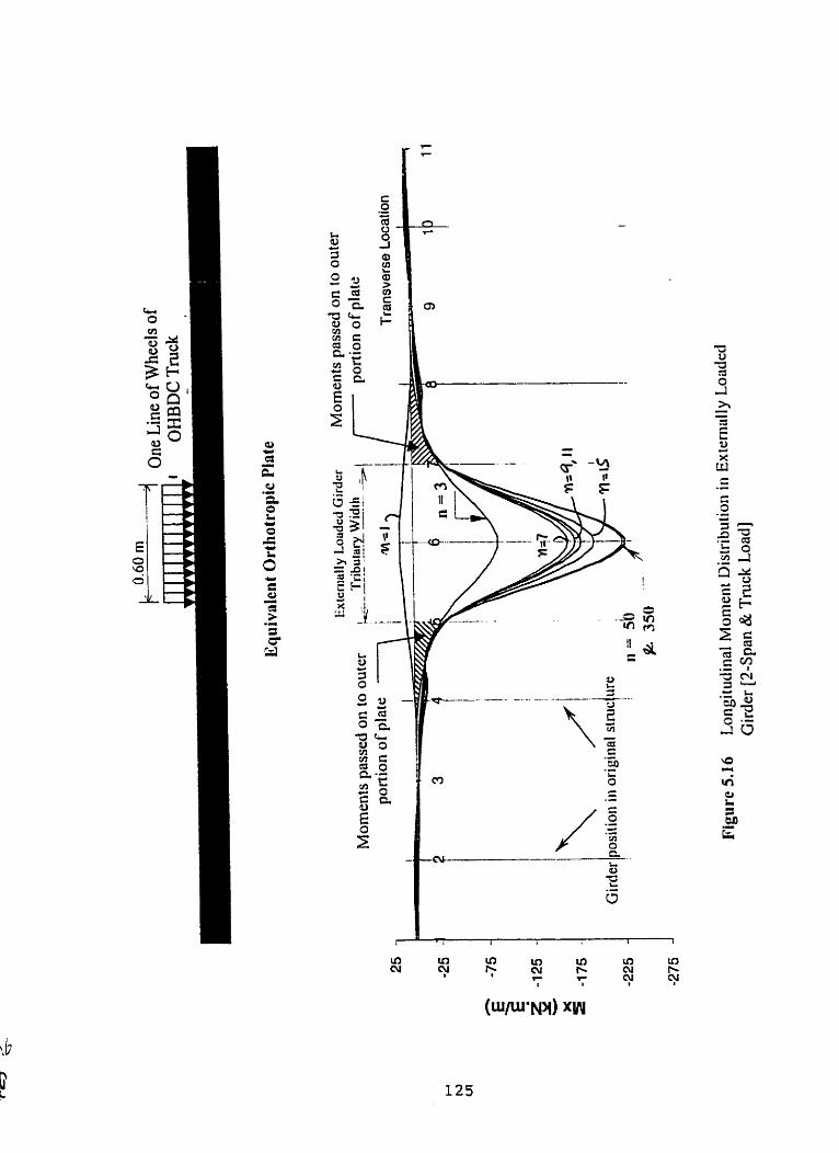
C'Y

Table 5.5 Values of My obtained bv PLAT0 at x = 1 5 rn, in kN.m/m
Longitudinal moment (Mx) computatiow in the ELG using 50 harmonies and the
-b
hastening technique are summarized below. MT in ELG using 50 hmonics , represented
by the area under My c w e was found to be -406.1 kN.m.
Table 5.5.1 Mx in ELG using Hastenkg Technique
I
1 2
Trans- Points "=l n=15 n=?l n=7
Total Free Moment ( M d
Moment in Outer Girders
2.4 -0.2
n=SO ~ 3 5 0 n=3 n=9
(Mo ) Moment in ELG
The results in above table show that the quick convergence scheme Ieads to more than
99% convergence of longitudinal moments afler considering oniy 9 hamionics.
=5
No. of Harmonies
(lW= (MF) - (Mo ) % Accuracv
5.3 -3 2 Convergence of Longitudinal Shears
The idealized isotropie plate was analyzed for longitudinal shears at x = 7.5 m using
2.9 1.5
3 1 -2.1
n = l -457.1 kN.m 6.37 kN.m -463.5
PLATO. The results are shown in Table 5.6 and plotted in Figure 5.17. Convergence of
shears in ELG is extremely slow as compared to longitudinal moments.
4 5
kN.m 87.6 %
0.3 9.0
n = 3 -457.1 kN.m -28.39 W.m -428.7
-8.4 , -3.3 ' -10.8 -11.0'
-2.0 -7.7 -31.8 -174.0 -31.8
43 ' 0.3 ' -3.O 1 -5.1 8.7
-2.0 -8.4 -31.6 -180.9 -31.6
6 14.8 7 1 9.0
kN.m 1 kN.m 94.7 % 1 96.7 %
1 7 - i . r
2.7 3.0
-2.0 -6.7 -31.9 -167.0 -31.9
2.8 2.3
i -1.8 1 -2.0 -3.0 1 -5.1 -27.1 ; -32.0 -89.3 ' -150.5
n = 5 -457.1 W.m -37.05 kN.m -420.0
2.8 2.7
2.7 3.2
-1.9 -9.3 -31.4
-193.9 -31.4 -27.1
kN.m 97.6 %
-32.0
9
n = 7 -457.1 kN.m -40.96 kN.m -416.1
kN.m 98.2 %
2.7 '
3.4 -1.9 -10.8 -31.4
-224.8 -31.4
n = 9 -457.1 kN.m -43.3 W.m 413.8
2.7 / 2.7 3.8 13.9
-1.9 -11.0 -31.4 -227.9 -31.4
-2.1 10 , -0.2
-3.9 3.4 2.7
-2.0 3.0 2.7
-1.9 3.8 2.7
-2.0 3.2 2.7
-1.9 3.9 2.7
-2.0 -1.8 2.7
11 / 2.4 , 2.9 ( 2 . 8
-2.0 1.5
2.8 2.3

One Line of Wheels of OHBDC Truck
Actud Slab-Girder Bridge
Equivalent Ortho-p lat e Rigidities n An rn W . V U LIl
Dr= 191.2E5 IcN.m, Dy=023ES kN-mk-4 One Line of meels of
OHBDC Truck - * -
Equivdent Orthotropic Plate
Externally Loaded Girder Tniutary Width
-30 1 Transverse Location
Figure 5.17 Transverse Distribution of Longitudinal Shear in Girder Bridge [Xpan & Truck Load]

Table 5.6 Vaiues of V, obtained bv PLAT0 at x = 7.5 m. kN/m - * l 1
a n=l 1 n=3 1 n=5 / n=7 1 n=9 / n i 1 ' n 1 5 n=50 i n=350 1 Points ; l I I I 1 1
1 ] 0.2 0.3 0.3 1 0.4 1 0.3 / 0.3 / 0.3 : 0.3 ' 0.3 2 0.0 1 0.4 0.1 -0.2 ! 0.0 0.2 i 4.1 ; 0.0 0.0 '
3 -0.2 -0.1 0.0 0.0 0.0 0.0 10.0 i 0.0 ; 0.0 '
Longitudinal shears in ELG cm be obtained as described earlier. The first harmonic
shears passed on to outer slab are shown by hatched are in Figure 5.18. Longitudinal
shear (V,) computations in the ELG are summarized below. V, in ELG using 50
hmonics. represented by the area under yr c w e , was found to be -16.94 W.
Table 5.6.1 b', in ELG using Hastenhg Technique:
No. of Hannonics 1
These results show that afier 1 1 harmonics, the quick convergence technique produced
98% convergence of results. It is observed that even after 9 harmonics the % accuracy
results are still oscillating. Although for the practical application of the hastening
technique. a virtually complete convergence c m be assumed if the consideration of
higher harmonics would yield a change in results of less than 0.1%. The study is
however? extended to observe the oscillation effects at higher harmonics. The results are
discussed in Appendix F.
l Totai Free Shear
( V F )
n = 5 43.28
kN
L
n =l 43.28
kN
n=15 43.38
kN 3 . 7 kN 46.99 kN
99.9%
n = 7 43.38
kN
n = 3 43.25
kN -2.75 kN 46.03
kN 98.1%
-1.70 kN
4 - 9 8 kN
-7.15 kN
50.42
Shear in Outer Girder (Y.)
Shear in ELG
n = 9 / n=ll
0 . kN
42.97
43.28 kN
-3.47 kN
46.72 kN = ) - ( O )
Oh Accuracy
43.25 kN
-4.60 kN
47.88 kN
9 5 . 8 % 1 9 9 . 5 % kN 1
91.5% (93.1% 98.0%

0.60 III One Line of Wlieels of
OHBDC Truck
Girder 1 si tiori in original structure \ I
Equivüleiit Oitliotropic Plute
, ~ x i e r n a l l y Loaded Girder i Tribuiary Width
Transverse Location
Figure 5.18 Longitudinal Shear Distribution in Extemolly Loaded Girder [2-Span & Truck Load]
5.4 Convergence of Results in Orthotropic Plate Method for Slab
Bridges
Slab bridges cm be idealized as isotropie plate that is a specific case of orthotropic plate
in which the longitudinal rigidities are equal to their respective counterparts in the
transverse direction. In girder bridges the concept of externally loaded @den is self-
explanatory. In slab bridges, however, the concept of the Externally Loaded Slab Strip
(ELSS) requires reflection. ELSS can be defmed as a longitudinal strip of deck slab
located under the loads and with a ~ ~ c i e n t width reflecting percentage of the total deck
width over which the harmonic variations are quite significuit. Moreover, the Poisson's
ratio considenbly affects longitudinal shear responses of the slab bridges. The width of
ELSS and the Poisson's ratio effects are explored in the subsequent sections. v
In order to illustrate the hastening technique in slab bridges three cases are studied, these
being: (1) a single span slab bridge under single central-load, (2) a single span slab bridge
with OKBDC truck Ioad. and (3) a two-span slab bridge under one line wheel of the
OHBDC truck loading.
5.4.1 Width of Externally Loaded Slab Strip (ELSS)
ELSS can be defined as a longitudinal strip of the deck slab located under the loads with
s a c i e n t width reflecting percentage of the total deck width over which the harmonic
variations are quite significant. =I'his is illustrated in Figure 5.19. ELSS represents the
portion of deck width beyond which two C u m e s , Say n = 5 and n = 350, are very nearly

the sarne. The concept of ELSS is signifiant because the effects of higher hannonics are
retained within this width.
ELSS = I
Figure 5.19 Definition of ELSS for Slab Bridges
It cm be observed frorn the results of various hypothetical cases discussed in the
subsequent sections that the ELSS for n = 1 and 350 was considerably wider than ihat for
n = 5 and 350. For practical purposes of defming ELSS, however. it was found
reasonably accurate io consider n = 5 and 350 for defining ELSS.
h o n g various factors that Muence wîdth of ELSS are ( 1 ) the aspect ratio of the deck
Le., the W/L ratio, and (2) the width v of the load-patch. These two factors are discussed
in the following sections.
5.4.1.1 Aspect Ratio E ffects
The effect of aspect ratio on longitudinal moments and shears is studied by the analysis
redts summarized in Tables 5 3 a ) and 5.7(b), respectively; these tables contain results
for aspect ratios of OS, 1, 1.5, and 2. The diEerent aspect ratios were achieved by keeping
bridge span as a constant at 10m and varying width as 5m, 10m, 15m, and 20m
respectively. The renrlts given in tables 5.7(a) and 5.7(b) were obtained for a single
patch load of 0.25m x 0.6rn, for mid-span moments and end-support shears. The ELSS
widths were then obtained fkorn iC& and V, plots and the greater of two values was
selected. These resdts are summarized in Table 5.10. It can be seen from this table that
for deck slabs of aspect ratios of 1 and higher, the ELSS, generally, falls within 35% of
the totaI deck width W.
5.4.1.2 Load Size Effects
The effect of load-size on longitudinal moments and shears was studied through the
analysis results surnrnarized in Tables 5.8 and 5.9. respectively: these analyses were
conducted for load-patch width of 0.25r1-1, O-Som, 0.75m, lm, 2x11, and 3m, for a bridge of
1Om span and 12.5m width. In ail cases. the length of the patch Ioads in the span direction
was kept constant at 0.25m. The ELSS widths were then obtained from il.!, and Y, plots
and the greater of two values was selected. These results are summarized in Table 5.1 1 . It
can be seen from this table that for most load cases with patch sizes of less than lm
width, the ELSS falls within 25% of the total deck width W. On the basis of above
anaiysis 25% of total slab width was assurned to be the width of ELSS for ail subsequent
analyses.

Table 5.7(b) Aspect Ratio Effect: Slab Bridge Response for
Table 5.7(a) Aspect Ratio Effect: Slab Bridge Response for Longitudinal Moments (LM,), in kN.m/m
Table 5.8 Patch
Longitudinal Shears (V,), in kNlm
Long
Trans. Points
1
w=20
Tram. Points
Size Effect: Slab Bridge Response for tuciinal Moments (1bf4. in kN.m/m
W=l 5 n=5
4.8
n =S
9.1
n=350
4.8
n=350
9.1 10.6 2 1 44.4
W=S
W=5
19.3
W=l O
44.6
n=5
43.4
1.5 1 1.5 i i 12.5 j 10.3 ! 5.5
R =l
19.3
n=5
17.9 10.6 1 6.2
n-350
43.5
5.1 2.8 i 2.8
W'lO ! W-15 n=350
n450
17.9 6.2
W=20 n=l n=t n=350 11-350 1 n=7 n-350

Table 5.9 Patch Size Effect: Slab Bridge Response for Longitudinal Shears (V,), in kNlm
Table 5.11 Summ;uv of the Effects of Load Widâhv on ELSS
Table 5.10 Summary of the Effects of Aspect Ratio (WIL) on ELSS
1 Load Width v 1 ELSS, m 1 ELSS, %W
Trans. Points
' Deck Span, m
5.42 Poisson's Ratio Effects
v =2m n-7 ( n-350
Jaeger and Bakht (1989) have discussed the effects of Poisson's ratio v and suggested that
the effect of Poisson's ratio on longitudinal moments and shears is extremely maIl in
girder bridges. In this study, however, it is found that in the orthotropic plate method,
v =3m n=l ( n=350
1 2 3 4 '
5 6 7 8 9
Deck Width, m (w)
V= 4m n=l 1 n=350
v c O25m
Aspect Ratio Wu
v = 0.5m ' v = 0.75m n-7 3.9 3.8
n=350 3.8 3.7
3.9 3.9
ELSS, m
4.3 / 4.0
n=f 3.9
10 1 3.8 1 3.7
ELSS, %W
n-7 n-350 3.8 1 3.9 3.8 1 4.0 / 3.8 1 4.2 1 3.9
5.5 7.5
3.8 3.8 1 3.7
n =350 3.8
4.7 5.4
4.7 15.5 1 4.7 / 5.5 5.4 j 7.5 1 5.4 / 7.6
ii ( 3 . 9 1 3.8
3.9 3.7 4.0
3.7 3 . 9 1 3.8 13.9 1 3.8 1 3.9 1 3.8 / 4.0 1 3.8 1 4.2
3.8 4.3
3.8 4.4
3.7 / 4.0 1 3.8 ! 4.2 4.0 1 4.5 i 4.1 ! 4.8
3.8 4.3
10.3
3.9 .
4.1 3.7 4.0
5.7 ( 9.9 1 5.7 j 9.6 1 5.7 9.3 1 5.6
5.5 1 4.7 1 5.8 1 4.7
3.8 / 3.7
7.6 1 5.3 6.1 1 4.6
- - 8
3 5.4 i 7.5 i 5.4 ' 7.6 ' 5.4 i 7.6 i 5.3 i 7.5 i 5.2 6.9 ' 5.0
4.0 1 3.8 ! 4.2
8.1 6-9
5.4 , 7.2 , 5.1 7.5 5.0
5.5 4.3
5.2
4.6 4.1 '
5.5 4.3
4.7 4.0
5.5 / 4.7 4.3 1 4.0
6.1 4.8
4.7 4.0
5.5 1 4.7 5.8 1 4.7 4.4 / 4.0 4.5 1 4.1

Poisson's ratio effects significantly affect the longitudinal shear response of slab bridges.
The accurate evaluation of the hastening convergence technique for slab bridges therefore
requires consideration of the Poisson's ratio effects. PLATO results for longitudinal
moment and shear responses of a typical slab bridge for v = O and 0.3 are shown in Tables
5.12, j.13, 5.14, and 5.15, for a patch-load of 0.25m x 0.6m and a bridge of van and
width of 10m and 12.5m, respectively. It is recognized that the Poisson's ratio for
reinforced concrete is rarely larger than 0.25. A value of 0.3 in the present study is used
to accentuate the effects of Poisson's ratio.
Table 5.12 PLATO results for mid-span Mx in a Single Span Slab Bridge [v = O], in luV.m/m
Table 5.13 PLATO results for mid-span Mx in a Single Span Slab Bridge [v = 0.31, in kN.m/m
n=9 Transg Points
n-5
12.6
n=50
12.6 12.6 1 12.6 1 12.6 1 12.6
n l l 1 il =15 n=7
12.6
n.=l
2 / 13.8 , 13.8 3 1 15.3 1 15.3 4 I 17.1 ' 17.1
n=9 Trans* Points
7
n=350
14.1
n=3
1 , 12.5
n=5 = n.3
14.1 / 14.1 i 14.1 1 14.1 14.1 ' 14.1 ' n.50
12.5
18.7 19.5 18.7 17.1 15.3 13.8
5 1 18.7 '
6 1 19.5
13.2 13.7 ----- 15.3 18.5 24.8
"=Il 17.7
1 2 3 4 5
n=350
1 1 / 12.5 1 12.5
7 8 9
n=15
13.2 13.7
18.4 23.8
12.9 1 13.2 13.3 1 13.7
14.51 16.5 / 18.1 19.3) 22.6
18.7 17.1 15.3
16.1 16.1 1 16.1 1 16.1 1 16.1 1 16.1
10 13.8
6 7 8
13.2 13.7 15.3
13.2 13.7 15.3
13.2 1 13.2
35.5
16.1
30.3 23.8 18.4 45.3 13.7
13.2 13.7 15.3
13.7 15.3
19.1 1 19.2 1 19.2 19.2 1 19.2
13.7 15.3
18.5 / 18.5 / 18.5
36.9 21.9 19.3 16.5
19.2 1 19.2 '
13.2
32.2 244 18.5
18.5 1 18.5 24.9
36.8 24.9124.9
27.4 22.6 18.1
9 1 14.5 ' 10 / 13.3
24.4
24.9
' 15.2 13.7 ~~~
23.6 1 24.2 1 24.5 ( 24.6 1 24.7 1 24.7 1 24.7
24.7 24.9 33.5 1 34.4
24.9
24.7 18.5
15.3 1 15.3 13.7 1 13.7
18.5 1 18.5 ( 18.5
27.4 1 29.2 1 30.4 1 31.4 1 32.5
24.8 18.5 15.3 13.7
15.3 1 15.3 13.7 ( 13.7 --- 13.2 113.2
23.6 19.1 16.1 14.1
33.9 1 33.9 24.7 1 24.7 19.2 / 19.2
15.3 13.7 13.2
1 12.6 1 12.6
16.1 14.1
24.2 / 24.5 j 24.6 19.2 1 19.2 i 19.2
___3------
16.1 14.1
24.7 19.2
12.6 1 12.6 12.6 ( 12.6 1 12.6
16.1 14.1
16.1 1 16.1 , 16.1 14.1 1 14.1 1
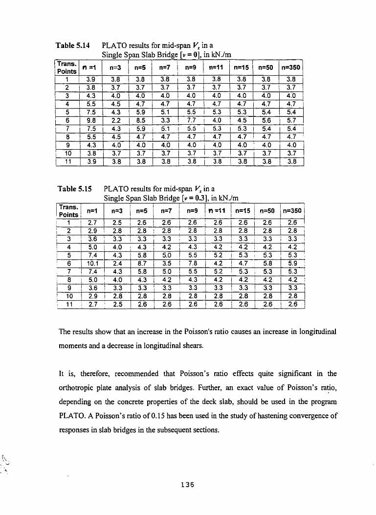
Table 5.14 PLATO results for mid-span Y. in a Singie Span Slab Bridge [v = O], in N J m
The results show that an increase in the Poisson's ratio causes an increase in longitudinal
moments and a decrease in longitudinal shrars.
Table 5.15 PLATO results for mid-span V' in a Single Span Slab Bridge [ v = 0.31, in kN./m
It is, therefore, recommended that Poisson's ratio effects quite significant in the
orthotropic plate analysis of siab bridges. Further, an exact value of Poisson's ratio,
depending on the concrete propenies of the deck slab, should be used in the program
PLATO. A Poisson's ratio of O. 15 has been used in the study of hastening convergence of
responses in siab bridges in the subsequent sections.
'
1 j n=q Points , 1 1 2.7
n=lS
3.8 3.7
1 n=J 1 n.5 n=7 n=9 n = r i I n=r s n.50 n=35o '
I I
Points n=50
2.5 1 2.6 1 2.6 1 2.6 j 2.6 i 2 1 2 - 9 1 2 . 8 1 2 . 8 1 2 . 8 1 2 . 8 2 . 8 2 . 8 1 2 . 8 1 2 - 8 1 1 3 1 3 . 6 ; 3.3 1 3 . 3 ; 3.3 1 3 . 3 j 3.3 / 3 . 3 i 3.3 1 3 . 3 1 1 4 15.01 4.0 1 4 . 3 : 4.2 1 4 . 3 1 4 . 2 i 4 . 2 ) 4.2 4 . 2 1
n =4 n=3
3.8
n.350
4.0 ' 4.0 1
2.6 i 2.6 / 2.6
j 5 ! 6
1 / 3.9
-
3.8 3.8 3.7 1 3.7
4.0 4.5 4.3
4.7 5.4
3 ) 4.3 4.0 1 4.0 i 4.0 1 4.0 1 4.0
' 6 1 9 . 8 1 2.2 1 8 - 5 1 3.3 1 7 . 7 i 4.0 1 4 . 5 ) 5.6 1 5 - 7 1 7 i 7.5 i 4.3 i 5.9 ! 5.1 i 5.5 1 5.3 1 5.3 1 5.4 5.4 1
n=S
3.8 2 / 3.8
4 . 7 ' 5.4
4 5
4.7 1 4 . 7 5.9 1 5.1
7.4 10.1
n=7 n=9 1 1
3.8 1 3.8 ) 3.8 3.7 ' 3.7
5.5 7.5
4.7 1 4 . 7 1 4.7 5.5 I 5.3 1 5.3
I
4.7 /
, 7 ( 7.4 a 4.3
3.7 1 3.7 3.7
4.7 8 / 5.5
4.3 1 5.8 / 5.0 1 5.5 l 5.2 1 5.3 1 5.3 5.3 j 2.4
4.0 i 4.0 ' 4.5
8.7 1 3.5 1 7.8 4.2 1 4.7 / 5.8 1 5.9 ' 5.2 1 5.3 1 5.3 1 5.3 5.8 1 5.0
8 1 5 - 0 1 4.0 1 4 . 3 1 4 . 2 ' 4.3 1 4 . 2 4 . 2 ; 4.2 1 4 . 2 1 1 9 3.6 [ 3.3 1 3.3 / 3.3 1 3.3 3.3 1 3.3 1 3.3 3.3
9
5.5
i 10
4.0 4.7 1 4.7 4.7 1 4.7 '
4.3 4.7
j IO '
2.9 / 2.8 1 2.8
3.7 4.0 1 4.0 1 4.0 j 4.0
3.8
2.8 1 2.8 i 2.8 1 2.8 1 2.8 2.8 ; 11 2.7 1 2 . 5 1 2 . 6
4.0
1 11 j 3.9
2.6 2 . 6 1 2 . 6 12 .6 12.6 12.6 -
3.7 j 3.7 1 3.7 1 3.7 3.8 1 3.8 1 3.8 1 3.8 1 3.8 j 3.8 1 3.8 3.8
3.7 / 3.7 3.7

5.13 Single Span Slab Bridge with Single Load
A single span bridge of span and width as s h o w in Figure 5.20 with a centrai load of 100
iu\i W Ü ~ anaiyzed using PLATO. The various parameters of this siab bndge and the
related plate ngidities are given below.
Span(L)= 10 m
Width (W) = 12.5 m Slab thickness (t) = 0.5 rn
E = 3 E 7 W / m 2
G = 0.87E7 kN / m'
Poisson's ratio u = 0.15
Flexurai and torsional rigidities D, = Dy = 1.08E5 kN.m
Coupling rigidi ties D, = D 2 = u D , = 3.12E4kN.m
Figure 520 Single Span Slab Bndge [Single Load]
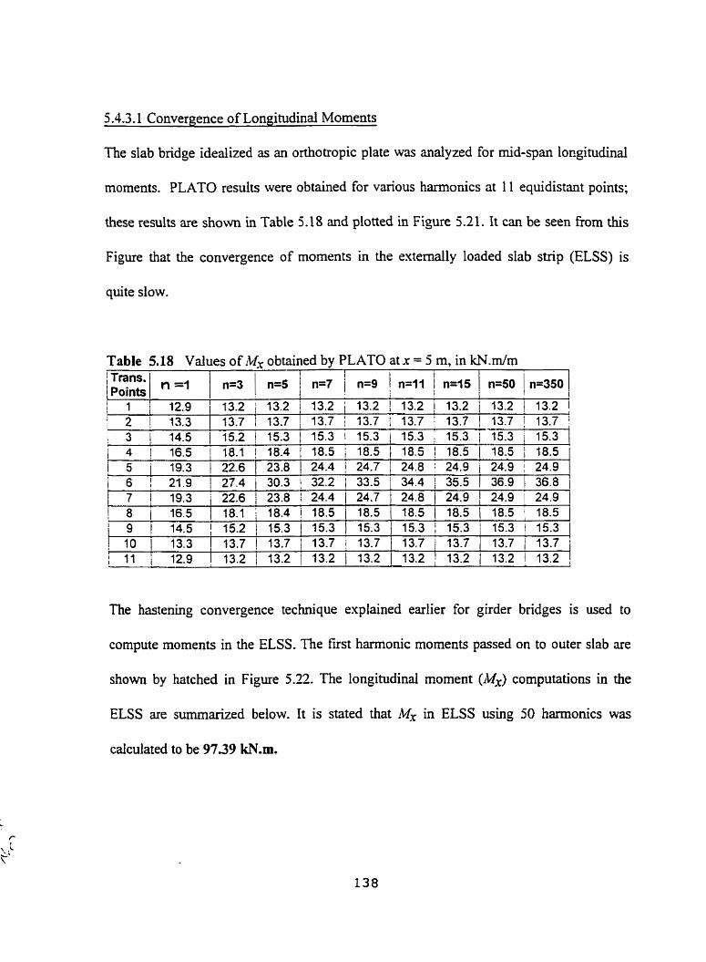
5 -4.3.1 Convergence of Longitudinal Moments
The slab bridge idealized as an orthotropic plate was analyzed for mid-span lorigitudinal
moments. PLATO results were obtained for various hannonics at 1 1 equidistant points;
these results are shown in Table 5.18 and plotted in Figure 5.21. It can be seen fiom this
Figure that the convergence of moments in the externally loaded slab stnp (ELSS) is
quite slow.
The hastening convergence technique explained earlier for girder bridges is used to
compute moments in the ELSS. The f ~ s t hannonic moments passed on to outer slab are
shown by hatched in Figure 5.22. The longitudinal moment (MT) computations in the
ELSS are summarized below. It is stated that & in ELSS using 50 harmonies was
cdculated to be 9739 W.m.
Table 5.18 Values of hl, obtained by PLATO at x = 5 m, in kN.m/m
czs / n =i 1 / 12.9 1 13.2 i 13.2 j 13.2 ; 13.2 1 13.2 / 13.2 1 13.2 / 13.2 j
, 2 13.3 / 13.7 1 13.7 1 13.7 1 13.7 i 13.7 1 13.7 1 13.7 ! 13.7 ' i 3 14.5 / 15.2 ] 15.3 1 15.3 1 15.3 1 15.3 ; 15.3 i 15.3 15.3 i 4 1 16.5 1 18.1 ! 18.4 1 18.5 1 18.5 1 18.5 / 18.5 1 18.5 / 18.5 / 5 i 19.3 122.6 123.8 124.4 ! 24.7 124.8 124.9 i 24.9 i 24.9
I n.3 1 n=5 "'7 j n=9 I n=1 I i 11.15 l !
n=so 1 n = x o

/
hctual Slab Bridge
Equivalent Iso-plate Rigities !
/ Dx=D"= : O.23ES kN.m 100 IdY
Equivalent Isotropic Plate
Externally Loaded SIab S trip ,+ z 35% of W
4 5 6 7 a Transverse Loaction
Figure 5.21 Transverse Distrîibution of Longitudinal Moment (M, ) in Slab Bridge [Single Load & Single Span]


Table 5.1 8.1 Mx in ELSS using Hastening Technique
The above table shows that the quick convergence scheme leads to more than 99%
Total Free Moment (MI-)
Moment in Outer Strip (w)
Moment in ELSS
convergence of longitudinal moments &er considering only 5 harmonies.
5.43 2 Convergence of Longitudinal Shears
The idealized isotropic plate was analyzed for longitudinal shears at s = O using PLATO.
nie results are shown in Table 5.19 and ploned in Figure 5.23. It can be seen that the
convergence of longitudinal shears in ELSS is much slower than that of longitudinal
No, of Harrnonics
moments.
Table 5.19 Values of Vr obtained by PLAT0 at x = O, in kN/m
n = 5 246.88 kN.m 149.06 kN.m 97.82
n = l 246.88 kN.m 138.53 kN.m 108.35
n = 3 246.88 kN.m 147.37 kN.m 99.51

/ ,
hctual Slnb Bridge
Equivalent Iso-plate Rigties ,/ DI= Dy= Dyx= 023E5 kN.m 100 kN
Equivrlent Isotropie Plate
Externaily Loaded Slab S trip + 2596 of W I = 3.125 m
-3-
u '
1 2 3 4 5 6 7 8 9 10 11 Transverse Location
Figure 5.23 Transverse Distribution of Longitudinal Shex (V, ) in Slab Bridge [Single Load & Single Span]
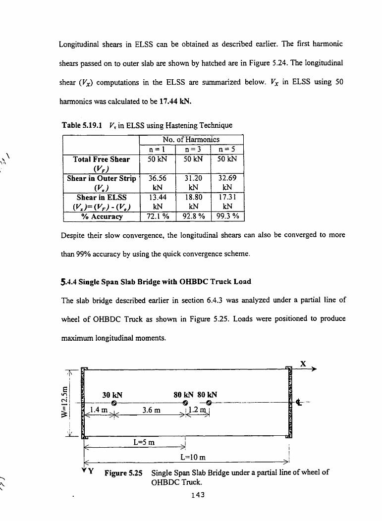
Longitudinal shears in ELSS c m be obtained as described earlier. The first harrnonic
shears passed on to outer slab are s h o w by hatched are in Figure 5.24. The longitudinal
shear (Y') computations in the ELSS are summarized below. V, in ELSS using 50
harmonies was calculated to be 17.44 kN.
Table 5.19.1 V, in ELSS using Hastening Technique
l No. of Harmonies 1 Total Free Shear
(Vd Shear in Outer Sbip
Despite their slow convergence, the longitudinal shears c m also be converged to more
than 99% accuracy by using the quick convergence scheme.
n = I 50kN
(vu) Shear in ELSS
5-44 Single Span Slab Bridge with OHBDC Truck Load
The slab bridge dexribed earlier in section 6.4.3 was analyzed under a partial line of
wheel of OHBDC Truck as çhown in Figure 5.25. Loads were positioned to produce
36.56
maximum longitudinal moments.
n = 3 50kN
kN 1 kN 13.44 1 18.80
P ,
y Figure 5.25 Single Span Slab Bridge under a partial line of wheel of OHBDC Truck.
n = S 50kN
31.20 IcN 17.31
32.69


5.4.4.1 Convergence of Longitudinal Moments
PLATO results for longitudinal moments are shown in Table 5.20 and plotted in Figure
Table 5.20 Values of 1& obtained by PLATO at x = 5 m, in kN.m/m r
m n s - 1 "=, 1 Points , n=3 1 n=S 1 "-7 1 n=9 1 "-11 ) " 4 5 1 n-50 1 11-350 1
Longitudinal moment ( ICI , ) computations in the ELSS using 50 hannonics and the
hastening technique are summm*zed below. The first harmonic moments passed on to
outer slab are shown hatched in Figure 5.27. Mx in ELSS using 50 hannonics = 130.05
- - . - - * - - .
Table 5.20.1 Mx in ELSS using Hastening Technique
Total Free Moment (MF)
Moment in Outer Strip (M. )
Moment in ELSS (M,)=(Mdo(M0)
% Accuracy
No. of Harmonies
n = l 370.5 kN.m
23 1.56 kN.m 138.94 kNm
93.6 %
n = 3 370.5 kN.m 239.07 kN.m 131.43 kN.m
98.9 %
n = 5 370.5 kN.m 240.42 kN.m 130.08 kN.m
99.9 %

One Line of Wheels of
0.5m OHBDC Truck
i
Actual Slab Bridge
P 4
Equivalent Iso-pIate Rigities 7 One Line of Wheels of 4 OHBDCTruck
. .
Equivalent Isotropic Plate
Externally Loaded Slab Snip ---+ G 25% of W / = 3.125 m -
1 2 3 4 5 6 7 8 9 10 1 1 Transverse Loaction
Figure 526 Transverse Distribution of Longitudinal Moment (MI ) in Slab Bridge [Truck Load & Single Span]


In the case of a single load, the quick convergence scheme led to 99.9% convergence
after 5 bmonics. As can be noted in the table above, the corresponding convergence for
multiple loads is improved to 99.9%.
5 -4.4.2 Convergence of Longitudinal Shears
The idealized isotropic plate was analyzed For longitudinal shears at x = O using PLATO.
The results are shown in Table 5.21 and plotted in Figure 5.28. Convergence of shears in
ELSS is extremely slow.
Table 5.21 Values of yr obtained by PLAT0 at x = O, in W l m
Longitudinal shears in ELSS can be obtained as desaibed eariier. The first hmonic
shears passed on to outer slab are shown by hatched area in Figure 5.29. Longitudinal
shear, y,, computations in the ELSS are nimmarized below. y, in ELSS using 50
harmonies was computed as 39.77 kN.
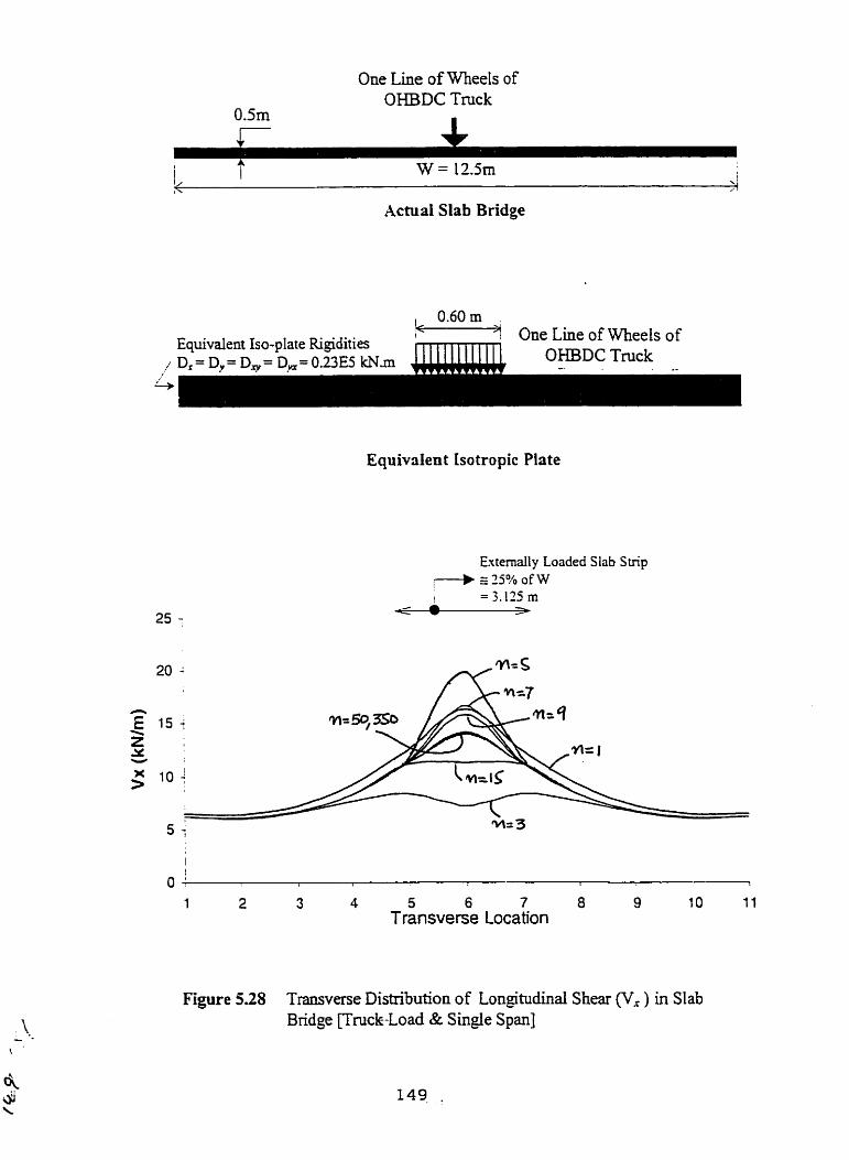
One Line of WheeIs of OHBDC Truck
0.5m
I W = L 2Sm l
I
1'
Actual Slab Bridge
0.60m . < .
Equivalent Iso-plate Rigidities OneLineofWheelsof OHBDC Tnick
Equivalent Isotropie Plate
Externally Loaded Slab Strip i-b z 25% of W
= 3.125 m i
1 2 3 4 5 6 7 8 9 1 O 11 Transverse Location
Figure 5 2 8 Transverse Distniution of Longitudinal Shear (V, ) in Slab Bridge [Truck-Load & Single Span]


Table 5.21.1 V, in ELSS using Hastenhg Technique
1 1 No. of Harmonies 1
1 Shearin ELSS 1 35.09 ( 43.57 1 39.43 1
Total Free ~ h e a r (V,)
Shear in Outer Strip )
5.4.5 Two Span Slab Bridge with OHBDC Truck Load
96.2 kN
61.1 1 kN
K)= (Vd - (Y,) % Accuracy
The slab bridge with a central support and loading as shown in Figure 5.30 was analyzed
using PLAT0 for longitudinal moments and shears. The results are discussed in the
96.2 kN
52.68 kN
kN 88.2%
following sections.
96.2 kN-
56.77 kN
Central Support
kN 91,3%
Figure 530 Two-Span Slab Bridge under a Partial Line of Wheel of OHBDC Truck
kN 99.2%

5 -4.5.1 Convergence of Longitudinal Moments
PLATO results for longitudinal moments at the transverse section containing the middle
support are shown in Table 5.22 and plotted in Figure 5.3 1.
Table 5.22 Values of iM, obtained by PLATO at x = 5 m, in kN.m/m
Trans. IPoints 1 =I 1 ni3 1 n=S 1 n-7 ( n=9 1 "=II 1 ~ = I S
Longitudinal moment (1CI,) computations i ~ . the ELSS using 50 harmonies and the
hastening technique are surnmarized below. The first harmonic moments passed on to
outer slab are shown hatched in Figure 5.32. iCI, in ELSS using 50 harrnonics,
represented by the area under Mx curve was found to be -2933 kN.rn.
Table 5.22.1 Mx in ELSS using Hastenhg Technique
1 No. of H
Total Free Moment -34.08 -34.08 (MLF) kN.m kN.m
Moment in Outer Strip -4.52 -2.45 w.0) m.m kN.m
Moment in ELSS -38.6 -31.63 (MX)= (MF) ' (Mo) mm kN.m
% Accuracv 76.0 % 92.7 %

One Line of Wheels of OHBDC Truck
Actunl Slab Bridge
0.60 m
Equivalent Iso-plate Rigities one ~ i n e of ~ h e e l s of
L D.==DY= Dr/= DF= O.23E5 kN.m OMBDC Truck
Equivalent lsotropic Plate
ExternalIy Loaded Slab Süip ,+ z 25% of W 1 = 3.125 m
Figure 5.31 Transverse Distribution of Longitudinal Moments (a) in Slab Bhdge
UN& L O & Ï & - T ~ O sPan]'


The convergence is relatively slow in a 2-span bridge. The quick convergence technique,
however, produces more than 99% accuracy after considering only 7 harmonies.
5.4.5.2 Converrrence of Loneitudinai Shears
The idealized isotropie plate was anaiyzed for longitudinal shears at .x = 2.5 m using
PLATO. The results are shown in TabIe 5.23 and ploaed in Figure 5.33. Convergence of
shem in ELSS is extremely slow.
TabIe 5.23 Values of P', obtained by PLAT0 at x = 2.5 m, in kN/m
Longitudinal shears in ELSS c m be obtained as descrîbed earlier. The first hannonic
shears passed on to outer slab are s h o w by hatched are in Figure 5.34. Longitudinal
shear (V,) computations in the ELSS are summ&ed below. V, in ELSS using 50
hannonics (area under y, curve) = -1 1.94 IrN

One Line of Wheels of ,
0 Sm OHBDC Truck
W = 12.5m
Actud Slab Bridge
0.60m K .
Equivalent Iso-plate Rigidities 4 One Line of Wheels of
/ Dx = Dy= D+*= Dm= 023E5 kN.m OHBDC Truck /' C -
Equivnlent Isotropic Plate
Extemally Loaded SIab S trip --+ 2 2594 of 1V
= 5.125 m - Transverse Location
Figure 533 Transverse Distribution of Longitudinal Shear (V, ) in Slab - Bridge Fmck Load & 2-Spanl
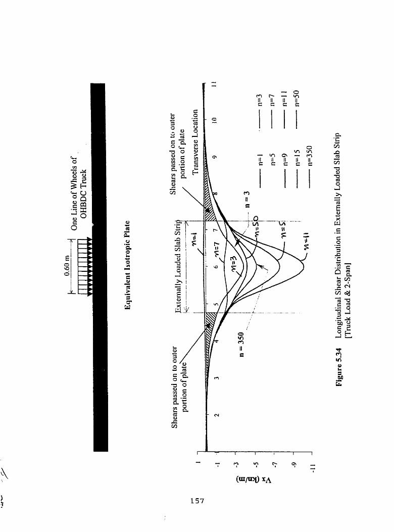
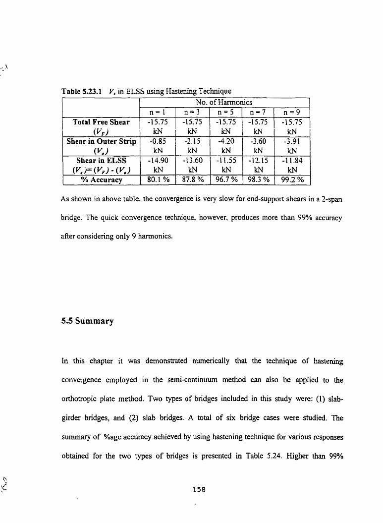
Table 5.23.1 V' in ELSS using Hastenhg Technique
- - - -
As s h o w in above table, the convergence is very slow for end-support shears in a Zspan
bridge. The quick convergence technique, however, produces more than 99% accuracy
after considering only 9 harmonics.
Totai Free Shear (hi
Shear in Outer Strip ( yo )
Shear in ELSS (Us (Vd - (5)
% Accuracy
5.5 Summary
In this chapter it was dernonstrated numericaily that the technique of hastenhg
convergence employed in the semi-continuum method c m also be applied to the
orthotropic plate method. Two types of bridges included in this study were: ( 1 ) slab-
girder bridges, and (2) slab bridges. A total of six bridge cases were studied. The
summary of %age accuracy achieved by using hastening technique for various responses
obtained for the two types of bridges is presented in Table 5.24. Higher than 99%
No. of Harmonies n = 1 -15.75
-0.83 kN
-14.90 Iù\J
80.1 %
n = 3 -15.75
icru' -2.1 5 IcN
-13.60 kN
87.8 %
n = 5 n = 7 n = 9 -15.75
k~ -3.9 1 ?LN
-1 1.84 kN
99.2 %
-15.75 -15.75 IÙ\I
4.20 kN
-1 1.55 kN
96.7 %
k~ -3.60 kN
-12.15 kN
98.3 %

convergence is shown in bold in this table. The results show that in most cases only five
harmonies are sufficient to obtain virtually complete convergence. Therefore, the
hastening convergence technique can be successfully applied to the orthotropic plate
rnethod to obtain quick convergence of various responses of the girder and slab bridges.
Table 5.24 Summw of % Accuracy using Hastening Technique in Girder and Slab Bridges
* Simply supported ** Two span

Chapter 6 Programs
PLATO and EDGE 6.1 Introduction
This chapter briefly reviews the modifications and improvernents made to the program
PLATO that incorporates a series solution of the orthotropic plate method discussed in
chapter 2. It further explains the technique that was used to cornpute edge beam moments
in slab-girder and slab bridges. Finally an addition to the program PLATO, called EDGE,
is prepared to generate edge beam moment results.
6.2 Program PLATO
6.2.1 Analytical Formulation
As it was discussed eariier in chapter 2, for orthotropic plate analysis the actual bridge
structure i s nnt transfomecl into an equivalent orthtropic plate and then using small-
deflection plate bendîng theories the goveming differential equations are denved. The
moments and shears are then obtained fkom appropriate differential expressions. Cusens

and Parna (1975) have derived expressions for moments and shean using patch loads as
shown below. It is important to note that these expressions use the equivalent hannonic
expression for patch loads as compared with point load expressions used in semi-
continuum method. By replacing point loa& with patch loads, the convergence of results
improves slightly due to term n appearing in the denominator of the equivalent hamonic
load expression.
The constants R,, 'K, 'K,, and x, are govemed by the relative position of the reference
station under consideration with respect to the Ioad. A schematic representation of the
computation process is shown in Figure 6.1.

Orthotropic Plate Method r
Patch Load Idealbtion i Deck S tructurc Idealization I Tnns formation Orthotropic Plate
4, Dy, D,,. Dy,. DI? D2 t
Plate lheorv
Deftection - I nxc , n m . n m
%Y),, - - sin-sln -in - .XI L L
Compute C PL' ' 1 nnc . nm
EvI,,,m =- s i n - - s i n -in - bn3 n3 L L L
PL' ' 1 nxc n m . nnu =-- C-pin- - s in - s i n -
bn3 n=, n L L
3 P L S 1 nxc nmc V,x,m=-- Zsin-cos+in
bnz "=, n L L L
- - Figure 6.1 Schematic Representation of the ShedMoment Computations in
Orthotropic Plate Method

Cusens, Pama and Robertson (1969) k t incorporated the computation scheme shown in
Figure 6.1 in a program 0BD3 using ALGOL for the ICL 4 130 cornputers. Later, Bakht
and Bullen (1975) produced a modified version of this program written Standard (ANSI)
FORTRAN for ICL 1900 and IBM 360/370 cornputers and was called ORTHOP, which
required fixed format input. Bakht has used the basic formulation of Cusens and Pama to
develop the program PLATO, which requires fiee format input and uses modren
FORTRAN language. A flow chart For this program is shown in Figure 6.2
6.2.2 irnprovements in the PLATO Output
One of the objectives of this project was to improve the output results generated by
PLATO. Output samples of the current as well as the improved format are s h o w in
Appendix C.
6.3 Edge Beam Moments
It has been shown by many researchers including Cusens and Pama (1975) that the effect
of introducing edge beam generaily improves the Ioad distribution characteristics of the
bridge deck provided that continuity exists between deck slab and the edge bean.
The existing version of the program PLATO takes into account the effect of edge bearns
by including flexural and torsional properties in the calculation of the coefficients.
However the analysis is LUnited to the extent that edge beam properties must be the same
on either side of the deck and by the assumption that the neutral axes of the slab and edge
bearns are coincident. A rectangular slab sirnply supported at two oppomte Sdes and fixed
or simply supported on the other two may be sîmulated by manipulating the edge beam
properties. The programPLAT0 however does not compute the bending moments M e

Calcula te ~ l l , b l i , C i l , dl1
~31,b31,~3ld31
Sll,Stl,S31>S.ll u Calculate
Calculute
Cslcufate MxNytMxy r M y x
V,,Vy, Den,
Subroutine II
t
Calculate M,,My,Mxy rMys
V,,V,, Defl.
Calculnte
Calculate
Subroutine
Calculate *KI,% u
1
Calculate Mi,My,Mxy,Myx
V,,Vy, Den.
Figure 6.2 Flow Chart for Program PLAT0 f

in the edge beam. It was shown in chapter 2 that the longitudinal moments L& in the
orthotropic plate are given by the following expression.
For small Poisson's ratio, the effect of coupling rigidity D, is very srnail and is therefore
ignored and Mx can be computed as
It was dso discussed in chapter 2 that fiom beam theory, the beam moment is computed 1
fiom following expression:
d 2 0 M,,, = EI-
d x2
If edge beam moment is represented by MW, the above equation can be written as:
d 2 m M e = EI-
d x 2

Now consider a point m that lies on the beam-slab interface Le., at y = O (or at y = W), as
shown in Figure 6.3. For compatibility requirements the rate of change of slope at point m
m u t be same for slab and beam at the beam-slab interface, therefore
Combining equations 6.1 and 6.2 yields
Figure 6 3 Typical Bridge Deck with Edge Bearns
In other words, the edge beam moment M,dge at any point on the beam-slab interface c m
be computed by simply multiplyhg moment M., as computed for orthotropic plate with
the t erm (E1/4,).

6.3.1 Program EDGE
The edge beam moments Medge at any point on the beam-slab interface cari be obtained
by modifjmg the program PLATO by incorporating equation 6.3. The resuiting program
is called EDGE and the flow chart for PLATO incorporating EDGE is shown in Figure
6.4. The listing codes for the modified pro- EDGE is provided in appendix A. The
program provides edge beam moments as well as other parameten including moments,
shears and deflection for the orthotropic plate as obtained for the point 'm' lying at the
common beam-siab intefiace as shown in Figure 6.3.
The prognm EDGE uses input and output files as discussed earlier for program PLATO.
It is important io note for specifjmg reference points (nref) the y coordinate is '0' for the
leA edge beam and 'W7 for the right edge beam. Sample input and output results for a
typical bridge exarnple are given in appendix B.
6.3.2 User Operation for EDGE
The edge beam analysis by using program EDGE is three-step process as explained
below.
1. The data-input to the program PL is created/modified, using any text-editor/word-
processor, in an input file calleci filename-dat. Any changes made in the input file

I Cull Subruutine
Calculate ~ I J z , Pl>P2 u
Subroutinc I-i Calculate
ro, P o
Calculate
Print X,Y,M, ,My,Mry ,My,
Vx,Vy, Dcfl.
V,,Vy, Defl.
Figure 6.4 Flow Chart for Program EDGE -

must be saved before ninning the program. The input parameters have the
fo llowing or der:
1. Title of the project
2. Bridge van (L), width 0, No. of harmonies (N)
3. D,? Dy, D,, D,? D,, D,
4. No. of edge beams (2), No. of columns (O)
5. E, 1, G, J (edge beam properties)
6. Magnitude of load (P), X-coordinate of load centre, Y-coordinate of load
centre, Length of load patch in x direction (u), Length of load-patch in y-
direction (v) . . . . [defuied for every load]
7. No. of reference points (nref). . .up to 50!
S. X-coordinate, Y-coordinate (nref pairs)
Any system of units can be used provided that they are consistent with each other.
2. The program is then r u simply by double clicking its edge-ere file in a window
mode (or by entering command edge at a DOS prompt). The program when nin
successfully show following messages:
S t a r t
reading data for PLATE & EDGE
data has been read
computing s t a x t e d in PLATE & EDGE BEAM
computing finished in EDGE
3. The results are stored in an output file called fiename.res. These results can be
viewed by double clicking this file in widow mode (this file can be opened using
any text-editor).
6.4 Summary
The application of the orthotropic plate method was extended to include moment
computations for the edge beams of slab-on-girder and slab bridges. Programs PLAT0
and EDGE are expected to be found useful in obtainhg the various responses of a @vert
bridge deck.

Chap ter 7 Conclusions and
7.1 Conclusions
The orthotropic plate method for rectangular plates supported on hnro opposite edges is
based on a series solution. The convergence of this method is slow especially for shears.
As many as 50 harmonies may be required to achieve Whially complete convergence. In
this study it has been demonstrated numerically that the technique of hastening
convergence employed in the semi-continuum method can also be applied to the
orthotropic plate method. The hastening technique is used to compute longitudinal
responses in single span and muiti-span slab-on-girder and slab bridges. The results show
that in most cases only 5 hmonics are sufficient to obtain virtuaily complete
convergence. The study m e r shows that this hastening technique is relatively
insensitive to the stiffhess characteristics of bridge decks.

7.2 Contributions
'Ibis study provides following contributions in the semi-continuum and orthotropic plate
methods of bridge deck analysis.
It provides useful data for the convergence of various responses in beams and bridge
structures under various load configurations.
It illustrates the use and application of harmonic series solutions for analyzhg single
and multi span beam structures.
The study aiso led to spreadsheet modules for the Manual Method of ana lmg slab-
on-girder bridge decks with five girders. Using these spreadsheets, design engineers
and researchen should be able to explore the 'What if situations and gain better
insight into the influence of the key variables.
The hastening technique illustrated in this study is expected to be found usehl in
obtaining longitudinal bridge responses more accurately and efficiently.
The modified program EDGE to compute longitudinal responses of edge beams is a
usefûl tooi. This will broaden the application of ûrthotropic Plate method in
obtaining accurate bridge deck responses.
7.3 Further Recommendations
Following recornmendations are proposed for further research.

1. The hastening technique illustrated numericdy in this study should be
mathematically incorporated in the PLAT0 program of the Orthotropic Plate Method.
2. For slab bridges, more work is required to accurately define and predict the width of
extemally loaded slab strip.
3. More research work is required to propose the technique of hastening convergence of
transverse responses.
4. In this study the spreadsheets are prepared for a 5-&der bridge. Work should also be
extended to cover practicai range of slab-on-girder bridges. This will increase
accuncy and efficiency of the klanual method of the bridge deck analysis.

References
1. Bakht, B., and Jaeger, L. G., (1985) "Bridge Anaiysis Simplifie&" McGraw-Hill
Book Co., New York.
2. Bakht, B., and Jaeger, L. G., (1986) "Analysis of bridges with intemediate supports
by the semi-continuum method," Proceedings, Annuai Conference of the Canadian
Society for Civil Engineering, Toronto.
3. Bakht, B., and Jaeger, L. G., (1990) "Semi-continuum analysis of shear-weak
grillages," Canadian Journal of Civil Engineering, 17(3), 297-301
4. Bakht, B., and Moses, F., (1988) "Laterai distribution factors for highwiiy bridges," J.
Stnict. Engrg., ASCE, 1 14(8), 1785- 1803
5. Bakht, B., Jaeger, L. G., and Casagoly, P. F., (1979) "Effect of cornputen on
economy of bridge design," Canadian Journal of Civil Engineering, 6 , 4 3 2 4 6
6. Bakht, B., Jaeger, L. G., and Cheung, M. S., (198 la) "Simplified d y s i s of cellular
and voided slab bridges," ASCE Journal of Structural Division, 1 O7(ST9), L797- 18 13
7. Bakht, B., Jaeger, L. G., and Mufti, A. A., (1996) ''Bridge Superstructures New
Developments," National Book Foundation, Pakistan
8. Bakht, B., Jaeger, L. G., Cheung, M. S., and Mufti, A. A., (1981b) 'The state of the
art in analysis of cellular and voided slab bridges," Canadian Joumd of Civil
Engineering, 8,376-391

9. Cao, L., and Shing, P. B., (1999) "Simplified analysis method for slab-on-&der
highway bridge decks," J. Bridge Engrg., ASCE, 125(1), 49-58
10. Cao, L., Shing, P. B., Woodham, D., and Allen, J. H., (1996) "Behavior of RC bridge
decks with flexible girders," J. Shct . Engrg., ASCE, 122(1), 1 1 - 19
1 1. Cusens, A. R., and Pama, R P., (1975) "Bridge Deck Anaiysis," Wiley, London
12. Hambly, E. C., (1 976) "Bridge Deck Behavior," Champman and Hall, London
13. Heins, C. P., (1982) "Applied Plate Theory for the Engineer," Lexington Books,
Massachusetts.
14. Jaeger, L. G., and Bakht, B., (1982) "The grillage analogy in bridge analysis,"
Canadian Journal of Civil Engineering, 9(3), 224-23 5
15. Jaeger, L. G., and Bakht, B., (1985) "Bridge analysis by semicontinuum method,"
Canadian Journal of Civil Engineering, 12(3), 573-582
16. Jaeger, L. G., and Bakht, B., (1985) 'The use of haxmonics in the semicontinuum
method of analysis of bridges," Cimadian Society for Civil Engineering Annual
Conference, Saskatoon, Sask. 83-97
17. Jaeger, L. G., and Bakht, B., (1989) "Bridge Analysis by Microcornputers," McGraw-
Hill Book Co., New York.
18. McFarland, D., Smith B. L., and Bemhart W. D., (1972) "Analysis of Plates,"
Macmilian Press Ltd., London.
19. Nagareda, Y ., and Takabatake, H., (1998) "A sirnplified andysis of elastic plates with
edge beams," Cornputers and Structures, 70(2), 129- 139
20. OHBDC (1992), Ministty of Transportation, Ontario

21. Smith, K. N., and Mikelsteins, L, (1988) cc Load distribution on edge stiffened slab
and slab-on-&der bridges," Canadian Journal of Civil Engineering, 15(6), 977-983
22. Szilard, R. (1974) "Theory and Analysis of Plate: classical and numerical methods,"
Prentice-Hall, Inc., New Jersey.
23. Timoshenko, S., and Woïnowsky-Krieger, S., (1959) "Theory of Plates and Shells,"
McGraw-Hi1 Book Co., New York.
24. Wang, T. L., and Haung, D. Z., (1992b) "Computer modelling analysis bridge
evaluation," Res. Rep. No. FWDOT/RMC/O542-3394, Florida Dept. of Transp.,
Tallahassee, Fla.

Appendix A Program EDGE
Listing Codes Program EDGE
REAL LOAD, 1, J,MU, Ki
ISTFGER Y,XX LOGICAL HB
COM'.ION / PLAT/ COL(21,6), HB, ICASE, L, El, SEXT, TCOEFF, TKNS, h XXyXXX(50) ,Y,YBB(SO) ,HBLDt:<YXrY'IYISPR,LOAD(41 5 ) & IUNIT, El, DXY, DYX, D I , Pl
COMMON / ADMIN/ IPAGE, LINE, MAXLIN, LUNIN, LUNOUT, ISCHRF(IO), ti IBRIRF(lO), IDATE(lO), JUNIT(l01, IHEAD(52,2), ITES(3), ISTOP, &
IMAGE(8O), JCASE(5)t LCNAME(lO), ICARD(11) IDEC COMMON / OVLY / IFIRST,IFMC,IFMR,IfML, IMNTIIRUN, IIIHB cha rac t e r+52 title IRUN=O MAXLIN=60 1 FIRST=l LUNIN=5 LUNOUT=80 OPEN(70, file='edge.datt) OPEN(80, fi1e='edge.resf ) write (6, + ) ' s t a r t ' write (6,*) ' reading data f o r PLATE & EDGE' read (70, + ) title write (80,110) t i t l o read ( 7 0 , * ) span, width, N write (80,120) span, width, N A=span/2 B=wFdth/2 read ( 7 0 , * ) DX, DY, DXY, DYX, Di, 02

! SHAHAB write (80,129) 129 format ( / 'Deck Slab Stif fness Prope r t i e s : ' ) write (80,130) DX, DY, DXY, DYX, DI, D2
! SHRWB read (70,') nedge, ncolumn ITES(2) = O L=ncolumn write (80,143) ncolumn if (nedge.ne.0) read (70,+) e t i,g, j
! S m & r i t e i ô û , 132) 132 format ( / 'Edge B e a m Properties : ' , !) write (80,133) e t if g, j 133 format ('E 1 G
! S HAHAB if (ncolumn.eq.0) go to 20 DO IO II = I, n c o l m n
10 read (70,') COL(II,1),COL(IX:,2),COL(II,3),COL(IS,4),COL(II,5),COL(II,6) 20 read (70, * ) nloads
y=riloads if incolumn,eq.O) go to 80 ITES (2) =O DO 50 TI = 1, ncolumn write (60,140)
TI,COL(ïI, L ) ,COL(11,2) ,COL(II,3) ,COL(II,4) ,COL(II,S) ,COL(II, 6 ) COL!~1,3)=C0L!II, 3! 12 COL(II,4)=COL!iI, 4 ) / 2
50 c o n t i n u e 60 c o n t i n u e
write ! 8 0 , i 3 5 ) nloads DO 30 II = 1, n l o a d s read ( 7 0 , * } LOAD(IIt1),LOAD(II,2) , LOFFD(II,3) ,LOAD(II,-!) , LOAD(11, 5)
30 write(80,~50)I1,L0AD(11,1),L0P.D(II,S),L3AD(11, 3),L0AD(11t4)tL0AD(11t5) read ( 7 0 , + ) neref XX=neref DO 40 II = L, neref
40 read (70, + ) 1 , YBB(I1) write ( 6 , * ) ' da ta has been read'
! SHMAB ! DO 80 11 = 1, neref ! 80 write (60, 160) II, LYX(TI), YBBIII) ! SHAHAB
c a l 1 PLATE write I70 , + ) ' computing finished'
i 1 C format(/'9ridge Project:',A) 120 format( / 'Span ( t ) ' , 5 x , 'Width (W) No. of harmonies
(n) ', /lx, F7-Zt5x, F9.Z,8x,I3) 130 format ( / ' D x DY DXY DY^ Dl 140 format (/'Col. No. x width
flexibilty settlement ' /5x, 13, 6x, & G(F9.4) )
143 format (/'No- of coiumns' , /5x, 3 3 ) 145 format (/'No. of loads',/Sx, 13) 150 f o r m a t (/ 'Load N o - Magnitude X-cor. Y-cor . x - d b . Y-
d i m . ',/lx, 13, 7x, &
F8-2, lx, F8.2, lx, f8.2, 3X, F7.2, 3X, F7.2,///)
D2'/6(E10.3)) breadth

SUBROUTIME ZERODY REAL 1, J , F I U , K I DOUBLE PRECISION M O , B10, SIO, S20, A0, BO COMON /.9LL/ALPN, B, DX, E, 1, EE, V, YC, YB, KI, KIN,VOVRB, ASl,ACl, BS1, BCl, & H,RfA,MU,RI,R2,D2,R3,R4,DY,G,J COE,iMON/WORK/FNl, FNA, FNB, FN4, FNS, FN6, FN7, -8, FN9, FN10, FNlA, E?!JIBf F N & FN14, FNl5, FNl6, FNl?, FNl8, FNl9, EY20, FN21fFN22, FNS3, FN24, FNîS, rN26 & , FN27, fillî8, FNZ9, FN30, E?J31f FN32, FN33, FN34, FN35, FN36, FN37, FN38, FN39, & W4O, FNdI, FN42, FN43, FN44, FN45, FN46, FN47, FN48, FN49, CN50,TlfT2, T3, T4 & ,TS,T6,T7,T8,T9,TIO,Tll,T12,TI3, Tl4 , T 1 5 , T l 6 , T 1 7 , T18,T'19,T20
! write (80,lOI) ! LOI format ('computing s t a r t e d in zerody ' )
BBO=ALPN+B+R FNlO=BBO+YB 1 (BBO-70 . ) 20,20,10
I C ) FEI2=1. FN3=I. GO T 3 30
20 rnB=FNE'T?. FNA= FNA'T2 FN3= ( fNB+FNA) - 0 . 5 FN2=FN3-ENA FNlB=FNlB"T3 FNlA=FNlA+T4 FN12= (FNIB+FNlA) +O. 5 FNl l=FN12-EWlA
30 FNl=E*IfPLPN/ (2 . + H W IF ( F N 4 LT. 1. E - 3 0 ) FN4=O. I F (rN5.LT.I.E-30) FN5=0. IF ( F N 6 . L T . l . E - 3 0 ) FN6=OI IF (FN7.LT.l.E-30) FM7=0. IF (FN8.LT.l.E-30) FN8=0. IF (FN9.LT.l.E-30) FN9=0. FN4=FN4 +TS FNS=FNS*T6 FNG=FN6*T7 FN7=FN7*T8 FN8=FN8*T9 FN9=FN9*TlO AIO=FN3+FNl*FN2 BlO=FN2+FNl+FN3 SlO=(i.-FNI) * (FN4-FN5) /R S20= (FEII-1. ) ' (FN6-FN7 ) /R AO=(SlO+S20) / ( 2 . 'A10) BO=(SIO-S20]/(2.+BIO) IF (BBO-70.) 5 O , S O , 40
40 CALL NOVFLO (AOfFN1O,BBO,ACl,AS1) CALL N O V ~ O ( B O , mm, BBO, BCI, BSI)

GO TO 60 50 ACI=AO*FNIS
ASl=AO*FNll 8Cl=BOf FN12 BSl=BO*FNIl
60 FNTI=FN8 IF (KIM.EQ. 1) FNTl=2.-FNT1 Kl=DX/ (4. * H t R ) * ( (FNT1-FN9) /R+ASI+BCI)
! write (80, 113) ! 113 format('computing f i n i s h e d in ze rody ' )
RETURN E?l E
SUBROUTINE PTLATE
1 NTEGER TEST, CT1, CT2
COMMON /-4LL/~PN,B,DX,E~I:,EEIV,YCIYB~K1,KIEII~?OvRBtASl, H,R,A,MU,Rl,R2,D2,R3,R4,DY,GtJ
COMMON / PLAT/ COL (21 , 6 ) , HB, ICASE, LI M, EIEXT, TCOEFF, TXNÇ, &
:<X,XXX(50),Y,YBB(50)IHBLDIXYXIYYYISPRrLOAD(4~,S)t &
IUNIT, El, DXY, DYX, Dl, M
CCMMOEI /ADMIN/ IPAGE, LINE, F l L I N , LUNIN, LUNOUT, 1 SCHEF ( 10) , &
TBRIRF(lO), IDATE(LO), JUMIT(lO},IHL4D(52,2),ITES(3), ISTOP, &
IMAGE(8O) ,JCASE(5} ,LCNPME(lO), ICARD(11), IDEC
DIMENSION TUM(9), SUM(9), TERPII(9) ,MAT(21,21), COMP(21) DIMENSION RUM(50,?) DIMENSION IFORM ( 5 ) , ITFORM(6) write (6,+) 'computing started in PLATE & EDGE B m S ' F= . F U S E , D= . F U S E . O=. F.9LSE. TEST=O PYE=3.141593 ALP=PYE/ (2. +A) N T Z = M I N O (50, ITES (3) ) IF (NTI.EQ.1) NTI=50 NB=N-NTl+l IF (NB) 10,10,20
10 N B = l NT l=N
20 NT=O IF (L.EQ.0) F=.TRUE. IF (Y.YQ.0) O=.TRUE. T=O

IF (MEXT.EQ.2) GO TO 210 IF ((ABS(BY)-l.E-4).LT.û.) GO TO 40 H={DXY+DYX+Dl+D2)/2. AL=H/SQRT ( DX'DY) GO TO 50
40 H=(DXY+DYX) /2. D= . TEIUE .
50 IF (ITES (2) ) 6O,8Of 60 60 Continue
IF ( D I GO TO 70 r . ~ q ~ m i ; i 0 7 r ~ . * - r v r n 7 -n t .r - # S b L U \ U U L Y W U A I 1 1 U 1 A ?
GO TO 80 70 WRITE (LUNOUT,780) 80 IF (N.NE.1) GO TO 90
N=5 T=l
90 MULTzlE-06 DX=DX*MULT DY=DYfMULT D1=DltMULT D2=D2*MULT E=E+MULT DXY=DXY'MULT DYX=DYX+MULT G=G'MULT H= (DXYiDYX+Dl+DS) /S.
! write (30,iOl) DX, DY, DXY, DYXI Dl, E2 ! 101 format ('six stifnesses', 6f10.1)
IF ( D ) GO TO 110 GLl=PJ,-I * IF (.&ES(-UI)-1.E-06) 120,100,100
100 IF (AL11 L401L20, 130 110 M=l
write ( 6 , + ) 'M=l' H= (DXY+DYX) /2. R=SQRT (DX/ ( 2 . 'H) )
GO TO 150 120 M=2
w r i t e (6,') 'M=2' GO TO 150
130 M=3 write (6, + ) 'M=3' R2=SQRT (H'H/ (DY'DY) -DX/DY) Rl=SQRT (R/DY+RZ) R2=SQRT ( H/ DY-R2 )
FNl=DY+R1*Rl-D2 F N 2 = D Y * R S + R 2 - D 2 FN3=FNI-DXY-DYX E'N4=FN2-DXY-DYX EW7=Rl*Rl.-R2'R2 write (6,*) ' j u s t before 140' GO TO 150
140 M=4 ! S P m
! w r i t e (6,*) 'M=4' ! SHAHAB
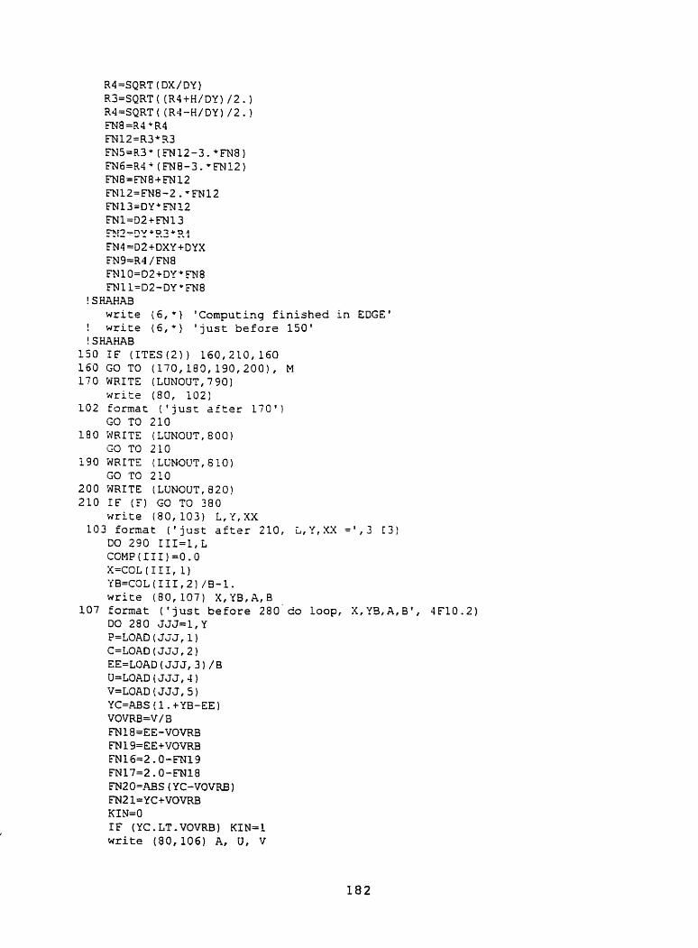
R4=SQRT ( DX/DY) R3=SQRT ( (R4+H/DY) /2. ) R4=SQRT((RS-H/DY)/Z.) FN8 =R4 + R 4 FN12=R3*33 FN5=R3+ (FN12-3. +E'N8) F N ~ = R ~ + m m - 3 . ~ ~ 1 1 2 ) FN0=FNS+E'N12 E'NIZ=FNB-2 .*FN12 FN13=DYtFN12 FNl=D2+FN13 fiI2-2Y + 9.2 '?.? FN4=DS+DXY+DYX FN9=R4 /FN8 FNlO=02+DY*E'N8 E'Nl L=D2-DY * ëN8
! S HAHAB write {6,+} 'Computing f i n i s h e d in EDGE'
! write (6,') ' j u s t before 150' ! SHAHAB
150 IF (ITES ( 2 ) ) 160t210, 160 160 GO TO (170t183, l9O,SOO), M 170 WRITE (LUNOUT, 790)
w r i t e (80, i02) 102 format ( ' j u s t a f t e r 1 7 0 ' )
GO TO 210 180 WRITE (LUNOUT,800)
GO TO 210 i90 WRITE (LÜNOUT, 8 10)
GO TO 210 200 WRITE (LUNOUT,820) 210 IF (F) GO TO 380
w r i t e (80 , 103 ) L, Y , XX 103 format ( ' j u s t a f t s r 210, L , Y , XX = ' , 3 13)
DO 290 III=l,L CGMP(III)=O.O x=coL(rrI, 1) YB=COL(III ,2) /B-1. write ( 8 0 , 1 0 7 ) X , Y B , A , B
107 format ('just before 280' d o loop, X,YB,A,B1, 4F10.2) DO 280 JJJ=l, Y F=LOAD (JGJ, 1 ) C=LOAD (JJJ, 2) EE=LOAD(JJJ, 3) / B U=LOAD ( J3 J, 4 ) V=LOAD f JJJ, 5 ) YC=PAS ( 1 - tYB-EE) VOVRB=V/ B FN18=EE-VOVRB EN19=EE+VOVRB E'Nl6=2 .O-FNIg FNl7=S .O-EN18 FN20-ABS (YC-VOVRB )
E'N2I=YC+VOVRB KIN=O IF (YC-LT-VOVRB) KIN=?. write (80 ,106) A, U t V

1 0 6 format ( 'A , U, V=' , 3FIO - 2 ) ECS=P/ ( 2 , +A+U*V) write ( 8 0 , 1 0 5 ) M, i?LP
105 forrnat ( ' j u s t before calling Fnexp, M, . U P = ' , 13, f10.2) CPLL INEXP (M,ALP) . U P N = O . wri te (80, 104)
104 format ( ' j u s t before 270 do laop') DO 270 Q=1, N AL?N=ALPN+ALF write (6,+) 'just before 220' 9 TC : 2 2 ! ? , 2 2 2 , 2 $ 2 , 2 5 2 ! , ?!
220 C U L ZERODY GO TO 2 6 0
230 CALL SLnA GO TO 260
240 C U L WLLF.4 GO TO 260
250 CALL SALFA 260 CONTINUE
GS=ECS/ALPNC '5'SIN (ALPNf O) +SIN (ALPNCC) 'SIN (ALPNCX) DEFL=Kl+G5/DX c o w ( r 1 r ) =COFIP (III) WL w r i c e ( 6 , + ) ' j u s t before 2 7 0 '
270 CCNTIMUE 280 CONTINUE 290 COE?P(III)=COMP(III)-COL(IIL,6) /E.IULT
DO 360 I I I = l , L ' f B = C O L ( I I I , 2 ) /B-1. X=COL(1I I , 1) DO 360 JJJ=l, L CE-COL (JJJ, 2 ) /E C=COL ( JJJ, 1 ) U=COL (JJJ, 3 ) V=COL (JJJ, 4 ) P=l.O YC=ABS ( 1, +YB-EE) W T (III, JJJ) =O ?iOVRB=V / B FN18=EE-VOVRB FN19=EE+VOVRB FN16=2.0-FN19 PNl7=Z,O-FNl8 FN20=nBS (YC-VOVRB 1 FN2l=YC+VOVRB K I N = O IF (YC-LT.VOVRB) KIN=1 ECS=F/ (2. +A*U+V) CALL INEXP (Pl, ALP) ALPN=O . write ( o f t ) ' just before do Loop 350' DO 350 Q=l ,N ALPN=.U,PN+ALP GO TO ( 3 0 0 f 3 1 0 , 3 Z 0 1 3 3 0 ) , 24
300 CALL ZERODY GO TO 340
310 CALL SLAB
GO TO 340 320 C U L TLALF.9
GO TO 340 330 CALL SALFA 340 CONTINUE
GS=ECS/ALPN*+S+SIN (.UPN* u ) *SIN (.;v,PN*c) +SIN (.ALPN*X) DEFL=KI *GS / DX MAT(IIIt JJJ)=M!T(III, JJJ) +DEFL
350 CONTINUE 360 CONTINUE
DO 370 ZI1=1, L 272 : . z y ; I z I , 111; G : . ~ T ; ~ Z ; , 111; +i-ûL <;ï; , 5 ; ,l;"iüLy
CALL GAUELI (L, MAT,COMP, DET, .TRUE. , W, TEST) IF (TEST-NE. (-1) ) GO TO 300 ISTOP=50 RETURN
380 IF (T.EQ.1) N=l LINE=200 KK=O
! write (80, L09)XX ! 109 format ('just before 670 do loop, X X = ' , 1 3 )
DO 670 III=L,XX :c=xxx ( II 1 ) YE=(YGB(III) -B) /B DO 390 Z = 1 , 9
390 TUM(Z)=O. CO 400 Q=l,YT1 [?O 400 2=1,7
300 RUM(Q,Z)=O.O IF ( L I N E + 1 0 - ? L U L I N ) -!2Ot4?.O, 410
410 CONTINUE TPAGE=I?AGE+I LINE=6 KK=O WRITE (LUNOUT, 8 60 1 LINE=LINE+9
420 CTI=L+Y ! w r i t e (80,111)CTI ! 111 format ('just before 620 do loop, C T I = ' , 13)
DO 620 JJJ=I, CT1 IF (JJ3.GT.Y) GO TO 430 P=LOAD (JJJ, 1) C=LOAD (JJJ, 2 ) EE=LOAD (JJJ, 3) /B O-LOAD (JJJ, 4 ) V=LOAD ( JJJ, 5 ) GO TO 440
430 CTZ=JJJ-Y P=-COMP (CT2) C=COL (CT2,l) EE=COL (CTS, 2) /B U=COL (CT2,3 ) V=COL (CT2,4 )
440 VOVRB=V/B DO 450 Z=1,9 SUM (2 ) =O

450 TEW(Z)=O YC=I\BS(l.iYB-EE) I F (YB+l.O.GT.EE) GO TO 460 K=-1 . GO TO 470
460 K = l . 470 IF (YC.LT.1.E-06) K=O.
FM 18=EE-VOVRB EX1 9=EE+VOVEIB FN16=2.0-FN19 FN17=2.O-rNl8 - , - , m - - - P . ,..- -.m..--.
c r 4 L U - M a [ L L ' V U V . s D f
FNSl=YC+VOVRB K I N = O 17 (YC.LT-VOVRB) KfN=l ECS=P/ (2. *A'U*V) C.XL INEXP (M,.9LP) .U,PN=O. NT=O
I write (80, 112) N ! 112 format ( ' j u s t before 000 do Loop, N=', 1 3 )
DO 600 Q=1,N .LPN=ALP?I+.4LP GO TO (480,490,500,530), X
480 C U L ZERODY ! write (80,124) Q ! 124 format('within 600 locp, z f t e r rzllinq zorcdy, G = ' , Ij)
X2=0. S'!K/R' (019-FN6) tACliES1) GO TU 5 4 0
490 CXLL ST&B FNTI=FM24 IF ( K I E l . E Q . 1) FNT1=-FNTI K2=O.25' (FMTl+mi30-FN2SCFN31+4SI+BSl+FN10+2. " K l ) i (3=0 .25 ' (KC( ( F N S 5 + l . 1 +FN31- (FNZ4tl. ) +FN~O)~AC~+BCI'FEI~O+BS~) K4=0.25+(K+((1.-FN24}CFN30-(1.-~25) ' F M 3 1 @ + 3 . * B S I ) GO TO 5 4 0
500 C;?LL W F A FNTl=FN34 FNT2=FN36 I F ( K I N ) 520,520,510
510 FNTl=-FNT1 FNT2=-FNTS
520 KZ=DX/ (2.O+DY+FN7) + (FNTl-FN3S-FNT2+E'N37+AC1*R1+Rl+BCl *R2*R2) K3=0.5/FN7*(K*((FN36-FN37)/Rl-(cN34-FN35)/R2)+ASl*R~+BSl~R2) K4=O.S/FN7*{K~((FN36-FN37)*R1-(FN34-FN35)*R2)+ASl+Rl+*3i6Sl*R2*~3) GO TO 540
530 CALL S&FA CNTZ=FN39 IF (KIN. EQ. 1) FNTl=-FNT1 K2=DX/ (4. *F'N2) + ( (FNTI*FN43-E'N41+FN44 1 - (ACl*FN12-2 .*BSl+ETJlS) *FN50- & (2. *AS1+FN15+BCl+E'N12) *E'N49) K3=0.25/FN15+ ( K / F N 8 * ( (R3* FN41fR4+FN42) f E 4 3 &
+ (MltR3+BC1+R4) +FN5O+ (BS1*R3-ACl*R4) 'FN49) K4=0.25/FNl5+ (K* ( (R4*FN4O-R3*FN39) f E ' N 4 3 - ( R 4 * 4 2 - R 3 4 ) 4 4 & 'FN5-9Cl*FN6) *FEISO+ (ACl+FN6+BSl+FNS) +FN49)
54 0 CONTINUE ! w r i t e (80, 1 1 9 ) Q

IF (M.NE.l) GO TO 550 F1=K1 F2=0.0 FS=DXY/ (2. +H) -- -4- *-*I I c i - c 5 n~
F4=-DYX/ ( 2 . +H) 'K2 F5=F5 'KI F6=F3 F7=0.0 F8=K2 F9=K1 /DX GO TO 560 Fl=KI-Dl/DX'K2 F2=- (DY/DX'KZ-D2/DXhK1) F3=DXY / DY'K3 F4=-DYX/DY+K3 F S = K l - (DYX+D1) /DXCK2 F9=K1/ DX F6=- (K4- ( D 2 t D X Y ) /DY+K3) F7=K1- (DYX+DXY+DI ) iDX'K2 FU=- (K4- ( D X * i + D Y X + D S ) / D m ) TERM ( 7 ) =F9+GS*bIULT T E W ( I ) = F I * G I TERM ( 2 ) =F2+G1 TERFI(3) =F3+G2 TERM (4 ) =F4+GS T E m ( 5 ) =F5 ' G 3 TERM (6) =F6*G4 DO 570 Z=1,9 SUMfZ)=SUM(Z) tTERX(2) IF (Q-NB) 600,580,580 NT=NT t 1 DO 590 Z='L,7 RUM(NT, Z)=SUM(Z) +RUM(NT, Z ) CONTINUE DO 610 2=1,9 TUM(Z) =TUM(Z) +SOM(Z) CONTINUE IF ( ITES (3) ) 630,650,630 DO 640 Q=I,NTI ROM ( Q I 7) =RUM (Qr 7) '1000. NT=NB+Q- 1 WRITE (LUNOUT,121) NT,iUU((III)rYBB(III), (RUM(Q,IJJ),IJJ=1,7) formar ('Label 64Q1, I3,1x, 9(ixIF11.4)) TUM(7) =TüM(7) '1000. 'WRITE (LUNOUT, 122) III,XXX(III) IYBB (III) 1 (TUM(JJJ) , JJJ=Ir7) format (lx,I3,1x,2F6.2,1x,7(Ix, 7E11.2))
! s w m w r i t e (LüNOUT,f) 'Edge Beam Moment a t r e f e r e n c e
point', III, ( fY+I) /DX) *TUM(T)

! S F - w LINE=LINO+I KK=KK+ 1 IF (,W-3) 670, 660,660
660 WRITE (LUNOUT,870) LIME=LINE+1 KK=O
670 CONTINUE IF (FI GO TO 750 IF ( (LINE+LO} .GT .MAXLIN) LINE=200 KK=O nn 7.tn 771-T T -v - 3 - uuu-J., u IF (JJJ-1) 680,690,680
680 IF (LINE+10-MAXLIN) 720,720,700 690 IF (LINE+15-YAYLIN) 710,710,700 700 Continue
IPAGE=IPAGE+l LINE=6 KK=O
710 WRITE (LUNOUT,880) SCNAME LINE=LINE+9
720 COLCOM=COL(JJJ, 5) +COMP (JJJ) ! WRITF ( LUNOUT, 1 FORM) JJJ, COMP 1 JJJI , COLCOM
LIEIE=LINEt 1 KK=KKt 1 TF iKK-3) 7 4 0 , 7 3 0 r ? 3 Q
730 WRITE (LUNOUT,$70) L I N E = L I F I E + I KK=O
7 4 0 CONTINUE 750 EIETtiRN
760 FORMAT (lXOt5OX, -!HDATA/IHO, 3Xr 4HN = ,13, 9X, 6HPYE = , lPE10.3,4Xt 4 W = &
, fPE10.3,4XI 4HB = , lPE10.3, 3X, 5HMU = , 1PEl0.3//4Xr -!HE = , lPE10.3 &
, 4Xt4HG = , 1?E10.3,4Xt 4HI = , lPE10,3,4X, 4HJ = , LPE10.3, 4Xt 4HH = , &
1PE10.3//3Xr 5 H D X = , IPE10.3,3X, SHDY = ,1PEl0.3,3Xf 5 F D 1 = ,1PE10.3, & 3X, 5HD2 = , lPE10,3,8H DXY = , lPEL0.3//8H DYX = ,1PE10.3)
770 FORMAT f 9H ALPW = , 1PE10.3) 780 FORMAT ( 9 H ALPHA = ,aHINFINITY) 790 FORMAT ( lH ,46X, 20HTHE ARTICULATE0 CASE) 800 FORMAT (1H , 47X, 18HTHE ISOTROPIC CASE) 810 FORMAT (1H , 31X, 'TORSIONXLLY STIFF AND FLEXURALLY SOFT BRIDGE DECK' ) a20 FOWT (IH ,~SX,'TORSIONALLY SOFT AND FLEXUENLLY STTFF BRIDGE DECKS') 830 FORMAT (IHO, SHICASE, 2Xt SHIUNIT, 6X, 2HE1, 7 X t 4 H T K N 5 , T C O E , 3 H L &
, 4X, lHY, 4Xt 2HXX/2Xr 13, 3 X t 13, 2X,ElO.3, F9. 3 , 2X, F8.2, 2 X t 3 (13, 2x1 ) 840 FORMAT (1H0,31HPATCH LOAD MRAY FOR HB LOADfNG/iH / (LX, I3,3X,Ell - 5 &
,2XtE1i.5,2X,E11.5, 2XrE11 .5,2XtE11.5) 1 860 format ( ' S t n . X-cor. Y-cor. Mx MY MxY MYX
Vx v Y DeEtlOOO ' , /, & 1 - - --- - - ------ ---- --- ------ ------- ----- -- ---- ------ --- -----
---- ------ ---- ------ - - - r ----- 1 ! 860 FORM24T ( / ' RESULTS FOR LOAD CASE - ' , / & ! '/'I STATION 1 CO-ORDINATES 1' &
! ,18X,7HMOMEMTS,18X,IHI,8X16HSHEARSr7Xt11 DEFLECTM II/' 1 NUMBER I*, &

! 4X, IHX, SX, l H I f 4 X f lHY, 5X, 1HI , b X , ~ H L X , 4Xf lHIf 4X, 2EMYf 4 X f 1H1, 4 X f 3HMXYf 3X, IHI, 4 X f 'MY ' , li ! 3X, 1HI,4X, ZHVX, 4X, LHf, 4 X f 2HW, 4 X f ' I ( + 1 .E-3! 1'/2H 1, 10 (10 (1H-),lHI) / )
870 FORMAT (lH )
! 880 FORM4T (/25H RESULTS FOR LOAD CASE - , / 'COLUMN W C T I O N S ' & / I ~ H (COMPRESSION +VE) / I ~ H O I COLUMN 1, LOX, IZHI ELASTIC r / &
' 1 NUMBER 1 REACTION I SHORTNG 1' 1'28 I f 3(10(1H-) , 1HI) /1HO) format ('results for colurnns') END
SUBROUTINE GAUELI (N, A, B, DET, FIRSTI, P, TEST) REAL A(21,Sl) , B ( 2 1 ) ,MAX INTEGER TEST, P(S1) ,CTl,CT2 LOG1C.A.L FIRSTI COMMON / AEMIN/ IPAGE, LINE, PDXLIN, LUNIN, LUNOUT, ISCHRF(LO), &
IBRIRF(lOl, IDATE(IO1, JUNIT(lO), IHEnD(52,2), &
ITES(3), ISTOP, IYAGE(80), JCASE(51, LCNnME(L0) , & ICPRD(ll), IDEC
IF (M.NE.1) GO TO 10 B (N) =B (N) / A ( M , M) GO TO 100 E=l , O CT I=N- 1 DO 130 K=L,CTI IF t .NOT.FIRSTI) GO ?'O 70 P ( K ) =K PAY=O. O DO 30 I = K , N I F (ABS(A(1,K)) .iE,MA>c) GO TC 20 KaX=ABS ( A I I , K) ) M= 1 CONTINUE CONTINUE If (kL4X.GZ.l.E-15) GO TO 40 XRITE (LUNOUT,i70) CkY,K TEST=- 1 DET=O . O GO TO 160 IF (M.EQ.K} GO TG 60 "--E u-
P(K)=M DO 50 J=K,N S=A (M, 3) A(M, J)=A(K, J) A ( K , J) =S CONTINUE CONTINUE M=P (K) IF (K-EQ.M) GO TO 80 S=B (K) B (K) =B (M) B (M) =S CT2=K+ 1 DO 120 I=CT2, N
S=A(I, K) / A ( K , K ) & ( I , K ) = A ( I , K ) / A ( K , K )
90 a ( I ) = B ( I ) - A ( 1 , K ) + B ( K ) I F ( . N O T . F I R S T I ) GO TO 1 1 0 DO 1 0 0 J=CTS,N
100 A ( 1 , J)=A(I,J) -S+A(K, J) 110 CONTINUE 120 CONTINUE 130 CONTINUE
IF ( F I R S T I ) DET=h (N, N) B (NI =B (N) / A ( N , N) 1 t & - L w - A
140 S = B ( I ) C T I = I + 1 DO 1 5 0 J=CTL,N
150 S=S-A(I,J)+B(J) B(I)=S/A(I, 1) I F (FIRSTI) DET=DETfA (1,I) I=I-1 I F (I.NE.0) GO TO 1 4 0 I F ( F I R S T I ) DET=DETfE
160 RETURN
17 0 FORK4T ( ' ZERO DIAGONAL ELEMEMT A R I S E S I N SIMULTANEOUS EQUATIONS . ' Ç
/30HCOEFFICIEMT W - T R I X IS SINGUM/22HP-a-THOLOGICAL PIVOT 1s , I P E l O . 3 &
, 15HARISING AT STFP, I-!) ZND
SUBROUTINE INEXP f M , AL?) REAL I I J , K l , M U COMMON /ALL/LLPN, B I DX, C f I r ZE, V, Y2, YB, K1 , KIN, VOVRB, AS1, ACI, B S 1 , Xi, & H,R,A,MU,RlIR2,D2,R3,R4, D Y , G , J COMMON/WORK/FNI, F A ( 1 1 ) f B ( 3 ) , FNI6, F N 1 7 , !3118, F Y l 9 , FN20, E N 2 1 F C 2 , r FD(4 ) ,TI,T2,T3,T4,Ts,T6,T7,T8,T9,T10ITll,Tl2,T3fTl4,T5~ T 6 , 1 7 , T 1 9 &
, T 1 9 , T 2 0
DO 1 0 1 1 = 1 , 2 5 10 F C ( I I ) = 1 .
BBA=l . GO TO ( 2 0 , 3 0 , 5 0 , 6 0 ) , M
20 BBA=R 30 DO 40 II=1, 11 40 FA(II)=1.
GO TO 7 0 50 BBA=Rl
BBB=R2*.UP+B F2=BBB1-YB T l l = E X P (BBB) TlZ=I./Tll T 1 3 = E X P (PZ) T14=1./T13 T l S = E X P (-BBBfE'N16) Tl6=EXP (-BBB"FN17) TlT=EXP ( -BBB*FNi8) T18=EXP (-BBB*FN19) T 1 9 = E X P (-BBB* E'N20 )

T20=EXP (-BBBf FN21) GO TO 70
60 BBA=R3 70 BBA=BBA+FLPf B
Fl=BBA*Ya TI=EXP (BBA) TS=I. /Tl T3=EXP (FI) Tq=I. /T3 TS=EXP (-BBA*FN16) T6=EXP (-BBAC FN17) 'r I=EXP (-BBA'FN18 )
T8=EXP ( -BBA+FN19) T9=EXP (-BBhtFN20) TlO=EXP ( -BBAtFN21) RETURN EN D

IF (FN28.LT.l.E-30) FN28=0- IF (EX29.LT.l.E-30) EN29=0. IF (FN30.LT.I.E-30) FN30=0. IF (FN31.LT.I.E-30) FN3t=O. FN26=FN26+T5 FN27=FN27'T6 FN28=FN28+ T7 FN29=FN29*T8 rN30=FN30+T9 FN31=FN31+T10 A2=FNIf FEJ2 bZ=r-q w r N 3 C2=FN1*FN3 DD=FN4 'FN2 A12=A2-B2 B12=C2-DO C12=BBN*A12+2.+FN3-DD D12=BBN+B12+2.+FNZ-B2 A32=C2+FN7*FN2 B32=A2+FN7 'ET13 C32=BBN*A32-FN8*FNS D32=BBN+B32-FN8'EY3 . aS=-ET?.I-FNI . 82=FEi2 6-FN27 C2=FN28-CE129 S32=(FN14+l. ) 'FM26- (FN15+II 1 *FFI27 Ç42=(cE122+1,) *cEl29- (FNSStI. ) +FM29 S12=A2+S32+FN8*82 S22=A2*S42+FE18*C2 A2=FN1-FN7 DD=2, - FN7 S32=A2'S32+DDhB2 S32=-A2+S42-DDfC2 C2=2.+(C12+832-C32'B12) DD=S.'(D12*A32-D32+A12) A2=( fS32+S42) '012- ( S M 2 2 ) tD32) /DD a2=( (s32-s42) ~ 1 2 - ~ ~ 1 2 + ~ 2 2 ) ' ~ 3 ~ 1 /c2 C2=((S12+S22)+B32-(S32-S42)tB12)/C2 DD=( (S12-S22) 'A32- (S32+S42) +,412) /DD IF (BBN-70.) 50,50,40
4Q CALL NOVFLO (A2, FETlO, BBN,ACl,ASl) CALL NOVFLO (ESt J3110, BBN, BClt BSI) CALL NOVFLO (C2,FNIO,BBN,CCl,CSl) C U L NOVF'LO (DD,FNlO,BBN,DCl,DSI) GO TO 60
50 ACI=A2*FN12 ASI=A2 * m l 1 BCl=BZ*FNIS BSI=BS*FNlI CCl=C2*FN12 CSI=C2*FN11 DCl=DD*FNIS DSI=DDfFN11
60 ASI=ASI+SCI ACI=ACl+BS1 BSI=CSl+DCl BCI=CCl+DSi

FNT1= (FNS4+2.) +FN30 I F (KIN-EQ-1) F N T 1 4 . - F N T l Kl=O. 25* (FNT1- (FN2S+2. ) *FN31+ASl+BSlfFN10) RETURN END
SUBROUTINE NOVFLO iXIN, EX1, EX2, XC, X S ) DOUBLE PRECISION XIN,XOT,Xl EOV=70. EX=EX 1 - EX2 -.- - I L = - I
XA=DABS (XIN) IO IF (XA-1.E-30) 40, 40f20 20 IF (ALOG (XA) +EX+EOV) 40t30, 30 30 IF (EX+EOV) 40,50,50 40 XOT=O. O
GO TO 60 50 XOT=XINfEXP(EX) 60 IF (II) 70,80,80 70 Xl=XOT
EX=-EXI-EX2 1 I=O GO TO 10
8 0 XC=Xl+XOT XS=Xl -XOT RETORM ZN D
SUBROUTINE SALTA REAL 1, J, MU, Xi DOUBLE PRECISIOM A13,B13, Cl3, D13,A33,B33, C 3 3 , D33, S l 3 , SZ3, 3 4 3 &
A3,83,C3, D3 COMMON /ALL/.qLPN, B, DX, Et 1, EE, V, 'fC, YB, KI, KIN, VOVRB, AS?. , AC1 ,9S I , BCI , S H f R,A,MU,R1,R2,D2,R3,R4,DYt G, J COC4PtON/WORK/FNl, FEI2, LN3,FM4, ëN5, FN6, FN7, FN8,rE19, FNlG, FN1L,9N12,FN13 & , ET114, FN15, FNl6, FN17,F'N18, FN19, FN20, m 2 1 , FN2A, FNZB, FN24, FM2S,FN26 &
, .W27, FN28, FNS9, ëN30, r-31, FN32, FN33, FEl34, FN35, FN36, M37, FN38, FN39, & FN4OfFN4I,FN92, E'N43,FN44,FN4A, FN4B,FN47,FN48,FN49,~SOtTItT2,T3,T4 &
,T5,T6,T7,T8,T9,T10,TIItT~2,TI3~T14~T15,T~6~T~J,T10,T19,T20

FhT4B=FN1BfT4 FN45=(FN4A+FN4B) + O , 5 FN46=FN45-E'NIfB
30 cN15=R3+R4 FN2S=COS (BB4) FN26=SIN (BB4) FN27=SIM ( B B 4 + F N 1 6 ) FN28=COS ( B B 4 * F N 1 6 ) FN29=SIN ( B B 4 + F N 1 7 ) FN30=COS ( B B 4 * F N 1 7 ) FN3I=SIN ( B B 4 + F N i 8 ) ?;12;CYS iZP3 ' FL<iô ; EW33=SIN (BB4*EW19) m 3 4 - C O S ( B B 4 * F N 1 9 ) I F ( F N 3 5 , L T . l . E - 3 0 ) FN35=0. IF ( F N X . L T . 1.c-30) m36=0. IF (FN37. LT. 1, E-30) FN37=O. I F (E'N38.LT.l.E-30) FN38=0. I F ( F N 4 3 , L T . l . E - 3 0 ) FN43=0. I F ( F N 4 4 , L T . 1 . E - 3 0 ) FN44=0. FEI35=FN35+T5 FEi36=FN30'T6 FM37=FN37CT7 FN38=FN38+T8 FN39=SIM ( S E 4 * F M 2 0 ) FN40=COS ( S B 4 * F N 2 0 ) FX4 l=ST:N (BB4+LN2 1) FN42=COÇ {BB4*FN21) FN4 3=FN4 3 +T9 FE14 4=FN44 " T l 0 FN47=SIM ( B B 4 *VOVRB) FN49=SIN (BB4'YE) FNSO=COS (BB4+YB) A3=FE123*FN25 B3=E'N24 *E'N26 C3=FN24'FN25 D3=E'N23+E'N26 A13=EYll*A3+2. + F N 2 + B 3 + F N 3 + (R3+C3-R4*D3] B13=FN1'D3-2.+FN2'C3+FN3'(R3+B3+R4'A3) C l 3 = F P l l + C 3 + 2 . +FN2+D3+FN3* (R3*,43-R4*B3) D13=FNl*B3-2. *FN2*.43+FN3' (R3CD3+R4*C3) S13=R3+FN4-DY+FNS S23=R4*FN4+DY*FN6 A 3 3 = S 1 3 * C 3 - S 2 3 * D 3 + E W + A 3 8 3 3 = S 1 3 + B 3 + S 2 3 * A 3 + W D 3 C33=S13*A3-S23*63+E'N7+C3 D33=S13*03+S23*C3+FN7*93 A3=FN3-R3/FN8*ENll 83=[R3*FN27+R4*FN28)*FN35-(R3*FN29+R4*EN3O)*FN36 C3=FN9*FNIO D3=(R3*FN31+R4+E'N32) *E'N37- (R3*FN33fR4*F%34 1 +ET38 S33=(R3*FN28-R4*FN27)*FN3S-(R3*E'N3O-R4*EW29)*F'N36 S43=(R3*FN32-R4*FN31) *FW37- (R3*FN34-R4*ETJ33) *EW38 S 1 3 = ( M * B 3 - C 3 + S 3 3 ) /FN8 S 2 3 = (A3*C3-C3'S4 3 ) /FN8 A3=2. *FN8'FN2-R4 *EN7 C3=FN7*R3-FN8*(FN13+FN4)

S33=(A3*S33-C3* B3) /FN8/FN8 S43=(C3*D3-A3*S43)/FN8/FN8 D3=2.'(A13+D33-A33*D13) C3=2.+(B13*C33-C13+B33) A3=( (Sl3tS23) *D33- (S33-S.33) *Dl31 /D3 B3=( (S13-S23) +C33- (S33+S43) *Cl31 / C 3 C3=( (S33+S43) '513- ( ~ 1 3 ~ ~ 2 3 ) W 3 ) /C3 D3=( (S33-S43) ' U 3 - (Sl3+S23) *A33) /D3 IF (BS3-70.) 50,50,40
40 C U L NOVFLO (A3, FN14,BB3,AC1,ASI) C U L NOVFLO (33,FN14,BB3,BCIfBSI) C U L NOVnO (C3, FN14,8B3, CC1, CSI) CALL NOVFLO (D3, FN14,BB3, DC1, DSI) GO TO 60
50 ACl=A3*FN45 ASl=A3*FN4 6 BCl=B3*FN45 BSI=B3*FN4 6 CCl=C3'FN45 CSl=C3* m4 6 DCi=D3* FN4 5 DSl=D3+FN4 6
00 ASl=ASI+CCl .Xl=ACI+CSI 9Sl=BSl+DCI BCI=BCI+DSI FNTl={2, +~15+FN40-FN124FE139i 'ET143 1 F (KIN.EQ. 1) FNT1=4 .+FN15-FNTI K I = C X / (4. 'F'P12) + ( (FNTI- ( S . ' n I15+F.142-
FN12-FE.141) ' F N 4 4 ) /FM8/FN8+AClCFN5O+BCltFN49) RETURN END
SUBROUTINE E U F A RE.= 1, J, MU, K1 DOUBLE PRECISION A1l,BIIf C1l,D11,43lt B3l,C31,D3L,S3lf S41, S 2 S l &
AI, BI,Cl,DC CONMON / X L / I U P N , 6, DX, E, 1, EE,V,YC, YB, Kl, KIEI,VOVRB,I\.SI,AC1, E E l f 6 C l , b
H,R,A,MU,R1,R2,D2,R3,R4,DYfG,J CûMMON~WORK/rN1,FN2,FN3fFN4,FN~fFN6,~7,FE18,FN9fFN10,FN11,FN12,F?.T13 h , FNl4, FN15, F N 1 6 , F N i 7 , FN18, E'tJI.9, FN20, FN21, FN2.9, FN2C, FNZB, FNSD, EX26 &
f~27,FN28,FN29,FN3O,FN31,FN32fFN33fFN34,FN3S,FN36,FN37,FN3A,FN3C, &
FN3B, FN3D, FN42, FN43,FN44, FN45,FN46,FN47,FN48,FN49, FN50,TlfT2,T3,T4 & fT5,T6,T7,T8,T9,T10~Tl1rT12~Tl3fTI4fT15fTl6fTl7tTl8~Tl9fT2O

20 FN2A=FN2AfT1 rN2B=FN2BfT2 FN22=(FNSA+FNZB) + O . 5 fl24=F'N22-FN2B E'N3A=FN3A*T3 FN3B=FN3B+T4 FN38=(FN3A+FN3B) *O .S FN4 O=FN38-FN3B
30 I F ( 8 8 2 - 7 0 , ) 5 0 , 5 0 , 4 0 40 FN23=1.
FN25=1. G ù T 0 b0
50 FN2C=FN2C*TI 1 FN2D=FN2D+T12 FN23= (FE?SC+FNZD) + O . 5 FN25=FN23-FN2D E'N3C=FN3Cf Tl3 FN3D=FN3D*T14 FN39= (FN3CtFN3D) *O. 5 FN41=FN39-FN3D
60 I F (FN26.LT.L.E-30) FN26=0. I F (FN27.LT.L.E-30) FN27=0. I F (328.LT. 1 .E-30) FN28=0, I F (FN29.LT. L .E-30) 3129=0. IF (FN3O. LT. 1 .E-30) FN30=0. I F (FN31.LT. 1 .E-30) FM31=0. 15' (FE132.LT. 1 . E - 3 0 ) ??132=0. I F ( F N 3 3 , L T . l . E - 3 0 ) FN33=0. I F (FN34,LT. 1.E-30) F N 3 4 4 . IF (FN35.LT. 1.E-30) F N 3 5 4 . IF (CN36.LT. 1 .E-30) E'N36=0. TF (FN37 .LT. 1 .E-30) FN37=0. FN26=FN26"ï5 FN27=!327 *T6 FN28=FN28 +T7 EN29=FN29+TS FN30=FN3OwT15 FN31=FN31fT16 E'N32=FE132*T17 EW33=FN33+T18 FN34=i?N34+Tl9 FN35=FX35"T20 FEI36=FN36*T9 M37=FN37+T10 All=FNL*FN22-~13+Rl+~24 Bll=FN2+FN23-FN13'R2'FN25 Cll=FNL'FN24-FN13*RltFN22 Dll=EW2'FN25-FNi.3+R2fFN23 A31=FN14+FN22-R1"FET3*FN24 B31=FNl4*F'N23-RZCFN4+FN25 C 3 l = r N l 4 * E ' N 2 4 - R I * F N 3 * ~ 2 2 D3l=FNl4*FN25-R2*FN4 +FN23 Al=(FN26-E'N27) /RI Bl=(FN28-M29)/R1 S31=(FN30-EN31) /R2 S 4 l = (FN32-FN33) /R2 S11=FNSCA1-E'N6*S31

S21=EX5*Bl-FN6*S41 Cl=FN3+FN14 /RI DC=FN4+FN14/RS S31=Cl*Fsl-DC+S31 S41=DC'S41-CI*Bl 81=2.*(A31~511-A11*531) DC=2~~(C31+Dll-Cll*D31) Al=( (S3l-S4l) '911- (SlIfS21) +B3l) / B l B1=((S11+S21)'A31-(S31-S41)*A11)/B1 Cl=( (S3i+S41) 'Dll-(Sll-S21) /DC OC=( (Sli-S21) 'C31- (S3ltS4I) *C1I) /DC IF (Z31-?2.; YV, Z2,fC
7 0 CALL NOVFLO ( A l , FN11, BBl,ACI,ASI) CALL N O V n O (Cl, FN1I,EB1,CCltCS1) GO TO 90
80 ACl=Al+FN38 ASl=AI+FN40 CCI=Cl*FN38 CS1=Cl+FN40
90 IF (BB2-70. ) 110,110,fOO 100 CALL NOVFLO (BI, FN12, BB2, BC1, ES1 1
CALL NOVFLO (DC,F?11S,BB2,DC1,DSl) GO TO 120
110 9Cf=B1*FN39 BS1=Bl*FN41 DCl=DC*FN39 DS1=DCf FN4 1
120 ASl=ASl+CCl ACl=ACI+CS1 BCl=BCI+DS1 ESl=BSl+DCI FNT'L=FN34 ENTS=FN36 IF (KIN) l 4 O , l 3 O , 130
130 ElITL=2. - F N T l FNT2=2 - -FNT2
140 K1=DX/ (2. 'DY'FN~) * ( (FNT1-9135) / R 2 / R 2 - (FNT2-FN37) /Rl/R1+ACl+Kl) RETURN END

Appendix B Program EDGE
Output

Stn. X-cor. Y-cor. Mx MY WY MYX Vx VY De£ *IO00 --- ---a ==st== ====== ------- ------- ------- ------- ------- ------- ------- ------- ------- ------- -- -----
---c--- -------- 1 0.00 0.00 0.00Et00 0.00E+00 0.23E+00 -0.23E+00 -0.88Et00 0.00E+00 0.00EtOO
Edge Beam Moment a t weference point 1 0.000000 2 7.50 0.00 -0.61E-i-01 0.17E+00 0.16Et00 -0.16Et00 -0.61Et00 -0.20E+OO -0.29E-01
Edge Beam Moment a t reference point 2 -15.7989 3 15.00 0.00 -0.85Et01 0.24E-1-00 -0.36E-07 0.36E-07 0.llE-06 -0.26E+00 -0.41E-01
Edge Beam Moment a t reference point 3 -22 ,1809
4 22.50 0.00 -0.61Et01 0.17Et00 -0.16Et00 0.16Et00 0.61Et00 -0.2OEtOO -0.29E-01 Edge Beam Moment at reference point 4 -15.7989
5 30.00 0.00 0.27E-05 -0.81E-07 -0.23E-t-00 0.23Et00 0,88E+00 0.34E-07 0.13E-07 Edge Beam Moment a t reference p o i n t 5 O . 702255E-05
6 0.00 12.50 O~OOE+OO 0.00Et00 -0.23E+00 0,23Et00 - 0 . 8 8 E t 0 0 O.dOEtOO 0.00E+00 Edge Beam Moment a t reference point 6 0.000000
F a 7 7.50 12.50 -0.61Et01 0,17E+00 -0.16E+00 0.16E-i-00 -0.61Et00 0.20Et00 -0.29E-01 00 Edge Beam Moment a t reference point 7 - 1 5 . 7 9 8 9
8 15.00 12.50 -0.8SE+01 0.24E-t-00 0.36E-07 -0.36E-07 0.11E-06 0.26Et00 -0.41E-01 Edge B e a m Moment at reference p o i n t 8 -23.1809
9 22.50 12.50 -0.61Et01 0.17E-t-00 0.16E-i-00 -0.16E-t-00 0.61E+00 0.2OE4-O0 -0.29E-01 Edge Beam Moment a t reference p o i n t 9 -15.7989
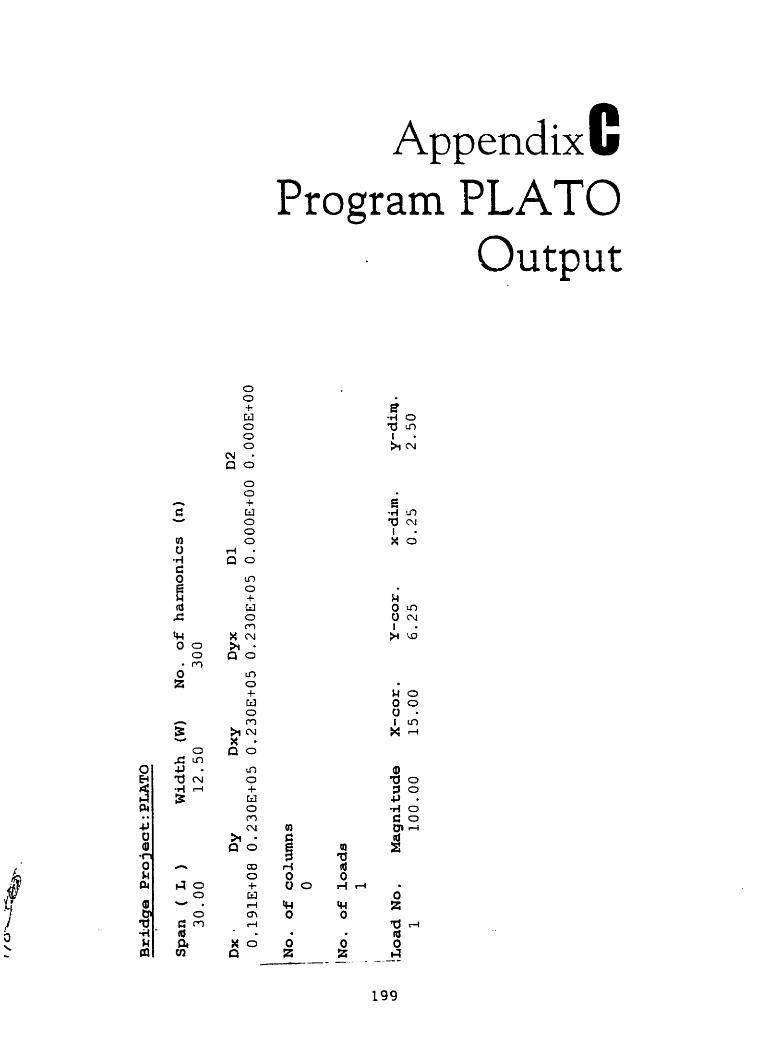
Appendix C Program PLAT0
Output

Def *IO00 S-=ri=====.
-0.90E-01 -0.4OE-O1 -0.15E-01
O. 10E-01 0.36E-01 0.62E-01
0,89E-01 0.12Et00 O.14E-t.00
0. 17Ei-00 0.20Ei-00 0.2 3E-te00
O.26EtOO 0.29Ei-00 O.X!E+OO
0.3LiEtOO O.38E+OO O.4OEtOO
O.4ZEtOO 0.44E-t-00 0.4 6E+-00
O, 47E-t.00 O. 48E-t-00 O. 48E4-00
O.48EtOO O. ri8EtOO O.48EtOO


Appendix E Effect of Load Width on
Hastening Process of Convergence
The technique of hastening convergence of the longitudinal shears and moments in slab-
on-girder bridges and slab bridges was explained in chapter 5. This section discusses the
effect of load width (v) on the process of hastening convergence.
The andysis results of PLAT0 of the longitudinal girder shears (V,) for the slab-on-
girder bridge shown in Figure 5.4 are provided in Tables El@), E2(a), E3(a) and E4(a)
for load widths of O.Zm, 0.4m. 0.6m and l.Om, respectively. These results are also plotted
in Figure E l . The computations for Y, in extemally loaded girder by using hastening
technique described in chapter 5 are shown in Tables El(b), E2(b), E3(b) and EJ(b) for
load width of 0.2, 0.4, 0.6 and 1.0m, respectively. These results show that the hastening
technique is relatively insensitive to the load widths of smaller than 0.6m. It seems that
relatively higher harmonies should be considered for load widths exceeding lm. From
practicai point of view, however, a load width of lm should be considered unredistic for
OHBDC trucks having a wheel spacing of 1 -8m.


Table E3(a) Values of V, obtained by PLATO at x = O m, kN/m lLoud size:0.25nr x 0 . 6 ~ 1
Table E4(a) Values of V, obtuined by PLATO at x = O m, kN/m fLoadsize: 0.25m x ln17
1
n = I n - 5 n = 9 n P 5 U np350 Pi.
1
V, in ELG using 350 harmonics = 17.42 kN
Table E3(b) V, in ELG using Hastening Technique I I n = ~ I r i = 5 1 r i = 9 1 n - 5 0 1 n = 3 5 0 1
Shcar in ELG v = v
Total Free Shcar (V,)
V, in ELG using 350 harmonics = 17.5 kN
Table E4(b) V, in ELG using Hastening Technique 1 I n - 1 1 r r - 5 1 n = 9 1 n = 5 0 1 n = 3 5 0 1
50.45 50.45 1 50.45 1 50.45 50+45
Total Free Shear (V,)
50,45
Sliear in Outer Girder (Vo)
Shear in (V,) = (VF) - (V',)
% Accuracy
32.85 1 32.78 ) 32.18 1 34,92 33,28
15.53
, 87.9%
17.17
97.2%
1 ~ 5 1 17.671 17.671
99.1% 100% 100%
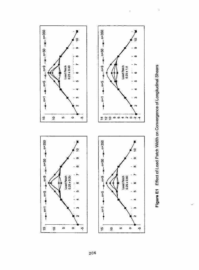
" O ?

Appendix F Oscillation of Convergence in a 2-Span Girder Bridge
The technique of hastening convergence of the longitudinal shears in a 2-span slab-on-
girder bridge was discussed in section 5.3.3.2. It was observed that the results were found
slightly oscillating after 9 harmonies. This purpose of this section is to observe these
oscillation effects in Longitudinal shears of 2-span bridge shown in Figure 5 - 1 4
[t is recalled that in order to anaiyze bridge decks with intermediate supports using
P L m , first it is required to obtain the reactions using well-known Force Method. The
structure is considered without intermediate supports and deflections are computed at
support locations using PLATO. The structure is then loaded with unit loads, one at a
time. at the intermediate support locations and deflections at each support location are
computed using progam PLATO. The following equation is then used to obtain final
support reactions.

Where, [6] is unit-load deflection matrk (5 x 5 ) and [A] is the deflection matrix (5 x 1)
obtained for the given structure without intermediate supports. These reactions are then
treated as negative loads in obtaining required responses using PLATO.
The analysis results of PLAT0 of the longitudinal girder shears (V,) for the slab-on-
girder bridge s h o w in Figure 5.14 are given in Tables Fl(a). The computations for V, in
extemally loaded girder by using hastening technique described are shown in Tables
F 1 (b).
These resuits show that oscillation effects are relatively small at higher harrnonics. From
practical point of view, however. considention of 9 harmonies should be considered
reasonably accurate.

Table Pl(a) Values of Y, obtained by PLAT0 at x = 7.5, in kN/m
V, in ELG using 350 (area under V' curve) = -79.17 IdY
Table E2 V, in ELG using Hastening Technique: n=l n=3 n=5 n=7 n=9 n = l l n=15 n=17
Total Free Sbcar -83.3 -83.3 -83.3 8 3 -83.3 -83.3 -83.3 -83.3 ( VP)
Shear in Outer 0.22 -8.27 -5.17 -2.60 -4.14 -5.61 -3.07 -4.07 Girdcrs
(V, )
% Accurncy 94.5% 94.78% 98,7"/0 98.1% 99.99% 98.13% 98.65% 99.92%