Have Absolute Price Levels Converged for Developed Economies? The

Evidence since 1870*

Lein-Lein Chen Department of Economics, University of Nevada, Las Vegas

Las Vegas, 89154 USA

Seungmook Choi Department of Finance, University of Nevada, Las Vegas

Las Vegas, Nevada 89154

John Devereux Department of Economics, Queens College, CUNY, Flushing

New York, New York, 11367-1597

Summary We compare price level and income convergence since 1870 for eleven developed economies using implicit price deflators derived from the GDP data of Maddison (1995, 2001 and 2003). We find that “sigma” and “beta” convergence for prices occurs later and to a lesser extent than income. Price levels converge after 1950 while income convergence begins in the 1880’s. We find no evidence for stochastic convergence or for “club” price convergence. JEL codes F3, F4.

Revised November 12, 2006 Forthcoming Review of Economics and Statistics

*We thank two anonymous referees and the editor whose comments greatly improved the paper. We also thank Marianne Ward for help with data. Devereux acknowledges assistance from the Center for Research in International Finance (CRIF) at Fordham University.

2

1. Introduction

Understanding the behavior of relative price levels is central to open economy

macroeconomics. Since the 1980’s research in this area has focused on testing for real

exchange rate stationarity and on estimating speeds of adjustment towards purchasing power

parity (PPP). Recently, however, interest has shifted to explaining absolute price levels (see

Taylor and Taylor (2004)). By absolute price levels, we mean price indices that measure the

relative cost of a basket of goods and services across countries at a point in time. The new

literature, for the most part, concentrates on the post-1950 era using data from the Penn

Tables. In contrast, the behavior of absolute price levels for earlier periods has attracted little

attention.1

We have two objectives in this paper. First, we introduce a rich new data set on long

run absolute price levels derived from Angus Maddison’s celebrated GDP estimates

(Maddison 1995, 2001 and 2003). Second, we test for price level convergence. As is well

known, income has converged for developed economies since 1870. Have price levels also

converged for these economies as suggested by standard trade models? To our knowledge,

there is no previous work on this question. Our empirical results show that price levels

converge later and to a lesser degree than income. As it turns out, price level convergence is

a post-1950 phenomenon while income convergence begins in the 1880’s.

We proceed as follows. Section two outlines how we construct our long run absolute

price indices using the implicit deflators from Maddison’s GDP volume indices. In total, we

1 Research on absolute price levels before 1950 is scarce. Bergin, Glick and Taylor (2004) test the Balassa Samuelson effect using long run absolute price indices based mostly on CPI and WPI indices. Friedman (1980) and Friedman and Schwartz (1982) study the UK/US absolute price level with implicit GDP deflators.

3

provide absolute price indices from 1870 to 2004 for eleven economies: Australia, Canada,

Denmark, France, Germany, Italy, the Netherlands, Norway, Sweden, the UK and the US.

Using Maddison’s price deflators, section three investigates price level convergence.

We begin by examining whether absolute price levels have gotten closer after 1870 as

measured by a decline in cross-sectional dispersion. This is “sigma” price level convergence.

Next, we test if countries with lower absolute price levels experience higher rates of dollar

inflation as implied by “beta” price level convergence. Using both sigma and beta measures,

we find that price levels converge later and to a lesser degree than income. Section four

introduces stochastic price level convergence. This investigates whether price levels move

together statistically. We find no support for stochastic convergence. Nor do we find

evidence for “club” convergence- a statistical co-movement of prices within a sub-group of

countries. Section five compares the results obtained from Maddison’s implicit deflators

with those from alternative absolute price indices. Section six concludes.

2. Measuring Absolute Price Levels

Angus Maddison (1995, 2001, and 2003) provides purchasing power parity adjusted

annual GDP data from 1870 to 2003 for a large sample of economies. His GDP data are the

standard source for empirical research on long run growth.2 To date, however, the implicit

GDP deflators implied by his volume indices have attracted little attention. We argue in this

2 The classic papers of Abramovitz (1986), Baumol (1986) and DeLong (1988) drew their inspiration from early versions of the Maddison data set. Since then virtually all work in the area relies on Maddison.

4

section that the Maddison deflators are the appropriate price indices if we wish to compare

income and price level convergence.

To set the stage, we outline how Maddison produces his GDP volume indices.3

Maddison begins by choosing 1990 as his base year. He forms his benchmark real GDP

comparisons using equation (1) where yi,1990 is the real GDP for country i in 1990 prices

expressed in dollars while Yi,1990 is the dollar denominated nominal GDP and pi,1990 is the

absolute price level of country i in 1990 prices obtained from the International Comparison

Project (ICP) of the United Nations.

(1) yi,1990 = Yi,1990/pi,1990

The next step is the crucial one. To generate real GDP for other years, Maddison

projects his GDP benchmark backwards and forwards with GDP growth rates taken from the

national accounts of each economy. Equation (2) gives the projected GDP series for country

i at year T, ,i Ty , where gi,T is the growth rate between the benchmark year and year T.

(2) ,i Ty = (1+gi,T) ⋅ yi,1990

Given that national income accountants calculate GDP growth using chained indices,

the GDP projections are also denominated in chained 1990 prices. The ratio of projected

GDP for any two countries is relative GDP in chained 1990 prices.

3 For details, see Maddison (1995).

5

The GDP deflator implied by Maddison’s real GDP index for each year is (3).

(3) , , /i T i T i T,p Y y=

Since the Maddison price deflators are dual to his GDP volume indices, the ratio of the price

indices for any two countries compares price levels at each point in time.

His most recent work (Maddison (2003)) provides annual real GDP estimates for

fifty-six economies from 1870 to 2003. We focus on eleven developed economies with, in

our view, reliable data. They are Australia, Canada, Denmark, France, Germany, Italy, the

Netherlands, Norway, Sweden, the UK and the US. Maddison does not report his implied

GDP deflators. Using (3), we can derive them from data on nominal GDP. Maddison (1992)

provides nominal data for Australia, Canada, France, Germany, the Netherlands, UK and the

US. For the remaining countries, we obtain nominal GDP from Maddison’s sources. Details

are in Appendix 1. The Maddison estimates end at 2003. We extend them to 2004 using UN

national account data.

We make one adjustment to Maddison’s real GDP indices. He compares GDP with

Geary Khamis price indices. Geary Khamis is a multilateral price index, which compares

price levels with a set of prices called “world prices.” These are constructed with data from

all economies, developing and developed. We prefer the Fisher Ideal index because it

compares income with data from countries in the sample.4 In addition, we need the Fisher

indices for our crosschecks in section five. The US is the base country throughout.

4 The Fisher indices are superior on theoretical grounds as they are superlative indices, see Neary (2004) who provides a definitive account of the Geary Khamis measure. Fortunately, differences between the 1990 Fisher

6

How accurate are Maddison’s GDP indices and their implied price deflators? This is

a difficult question that we discuss at greater length in section five. The consensus among

economists is that Maddison’s GDP estimates, the result of a lifetime of painstaking work,

are the best available. As mentioned, empirical research in long run growth, trade and

history relies on them almost exclusively. At a minimum, therefore, his implicit price

deflators are the natural starting point for the study of long run absolute price levels,

particularly when comparing price level and income convergence.

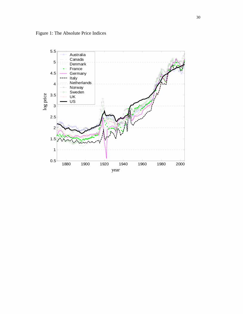
Turning to the data, Figure 1 graphs the log of the absolute price index for each

economy from 1870 to 2004. As we might expect, there is rough price stability for the Gold

Standard. The fall in price levels for early years is followed by a rise in later years. After the

First World War, dollar price levels rise. They decline in the 1920’s and early 1930’s with

dollar deflation. From 1940 onwards, we see sustained dollar price increases with evidence

of a return to price stability in the last decade.

Are price levels for developed economies getting closer over time? Figure 1 suggests

that there is price level convergence but only for later years. The next section explores the

issue in more depth by looking at sigma and beta convergence while section four provides a

more formal test of price level convergence.

and Geary Khamis measures are small for the economies in this study. The average difference between the two measures is three percent.

7

[INSERT Figure 1 around here]

3. Sigma and Beta Convergence

Sigma price level convergence occurs when there is a decline in the cross sectional

dispersion of absolute price levels over time. To determine if price levels have experienced

sigma convergence, we plot in Figure 2 the cross-sectional standard deviation of absolute

price indices measured in logs. To allow for a comparison with income, the first panel

provides the dispersion of the log of income per capita.

[Insert Figure 2 around here]

We begin with income. In line with previous findings, Figure 2 shows rapid sigma

income convergence. The standard deviation of the log of income falls steadily from 1880 to

1980. The exception is the period surrounding the Second World War where output

collapses for some combatants. From 1880 to 1980, the standard deviation of income

declines from 0.35 to 0.11, a reduction of two thirds. After 1980, income convergence

ceases.

Panels (b) and (c) provide the standard deviation of the log of the absolute price

indices. Panel (b) traces the standard deviation of the raw price indices while panel (c) gives

the standard deviation of prices filtered by the Hodrick Prescott (HP) procedure (Hodrick and

Prescott, (1997)).5 We use the HP filter to smooth out transitory movements in dollar prices

5 We set the weight parameter λ = 100 for the HP filter.

8

resulting from large exchange rate changes associated with wars, hyperinflations and floating

exchange rate periods.

Figure 2 shows that price level dispersion behaves differently from income. Most

notably, it falls later and to a smaller extent. During the early 1880’s, the beginning of the

classical Gold Standard, the standard deviation of log prices is around 0.23. In contrast,

income dispersion is 0.35. Price level dispersion increases slightly before 1913. Between

1914 and 1950, dispersion is volatile with the First and Second World Wars and the German

inflation.6 By 1950, the standard deviation of the log of prices is 0.28. From then on

dispersion declines. By the early 1960’s, the standard deviation of prices is 0.23- back to its

level during the early Gold Standard. There is a further decline from 1978 to 1994. This is

followed by an increase to 2004. For 2004, the standard deviation of price levels is 0.17,

which is twenty-five percent below its level during the early Gold Standard. The standard

deviation of the log of price levels for 2004 exceeds that for income by about forty percent.

The behavior of price level dispersion is puzzling in the light of theory. The

traditional models of relative price levels, the Balassa-Samuelson model (Balassa (1964) and

Samuelson (1964)) and the factor proportions model (Ohlin (1933) and Bhagwati (1984)),

show that price levels are determined by technology and factor endowments respectively.

These models predict that income and price levels should converge in tandem. As we have

seen, the rapid convergence in output from 1870 to the late 1930’s did not lead to price

convergence. The failure of prices to converge between 1880 and 1913 remains surprising.

The absence of sigma price level convergence from 1914 to1950 is, however, attributable to

6 Figure 1 shows that the decline in dispersion for the early 1930's is because of the temporary dollar depreciation of these years.

9

the breakdown in financial and trading arrangements during these years. In particular, the

retreat from globalization likely increased the dispersion of traded goods prices.7 Along

similar lines, trade liberalization and the move to convertibility after 1950 may explain some

of the price level convergence of the 1950’s.

Next, we consider Beta price convergence. In the growth literature, beta convergence

states that countries with higher initial income levels will experience slower rates of growth.

For prices, beta convergence requires that the higher the initial absolute price level, the lower

is the inflation rate measured in dollars. Given our finding of sigma convergence, we also

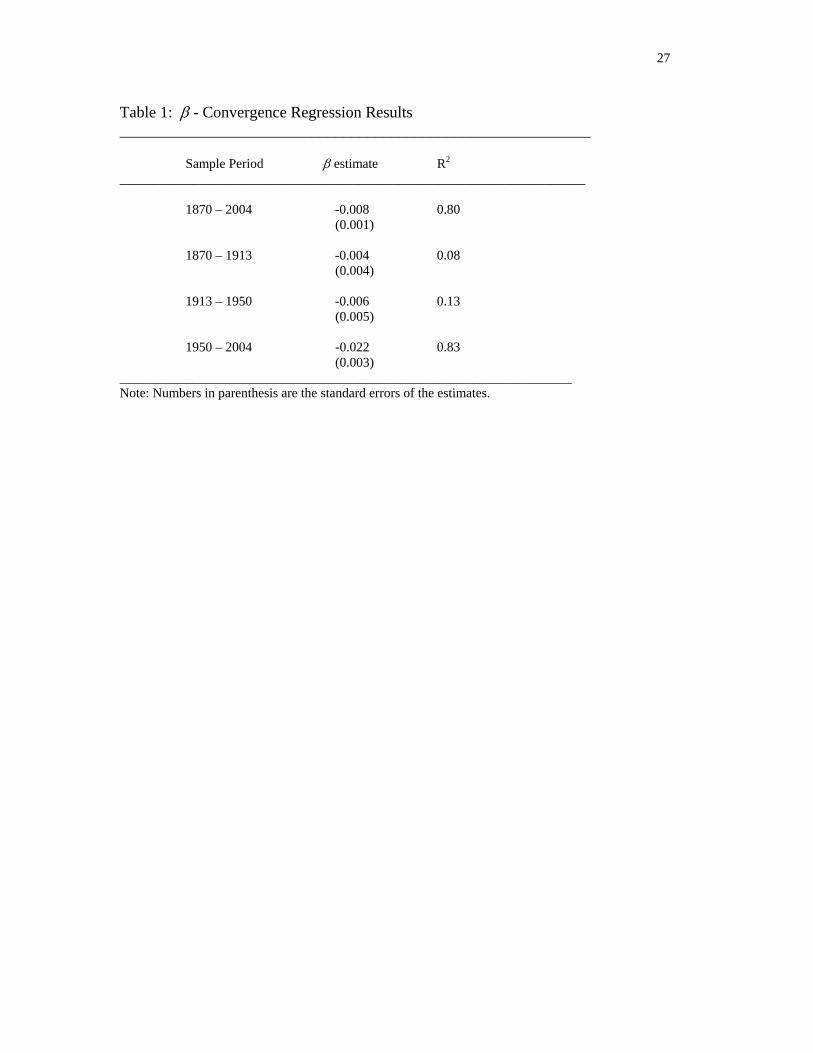
expect to find beta convergence. This turns out to be the case. We test β− convergence with

the following model: 8

(4) ( ) ( ),, ,

,

ln lni Ti t i t

i t

pT t p

pα β ε

⎛ ⎞− = − ⋅ +⎜ ⎟

⎝ ⎠,

where subscript t and T are the beginning and ending year of the sample period respectively.

The dependent variable is the average annual dollar inflation rate over (T-t) years.

[Insert Table 1 around here]

7 Obstfeld and Taylor (2004) discuss reduced economic integration during the interwar years highlighting the greater dispersion of real interest rates and the decline in the volume of trade. Real wages also diverged, see O’Rourke and Williamson (1999). 8 As is well known, beta convergence does not always imply sigma convergence. In practice, however, they are closely related. It is also standard to estimate (4) using a non-linear procedure see Sal-I-Martin (1996). We use simple OLS because of our small number of observations.

10

Table 1 summarizes the results for standard sub-periods, 1870-1913, 1913-1950 and

1950-2004. The results are consistent with earlier finding that sigma price level convergence

is a post-war phenomenon. For the overall period, 1870-2004, the estimate for the β

coefficient is statistically significant. Of the sub-periods, however, only1950-2004 shows

beta convergence.

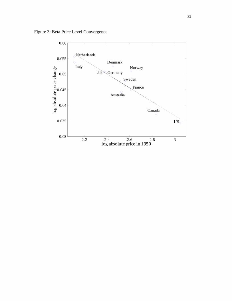
We plot in Figure 3 the relationship between initial price levels in 1950 and

subsequent dollar inflation. It shows that countries with high price levels in 1950 such as the

US and Canada experience lower dollar rates of inflation as compared to countries with

lower price levels such as Italy.

[Insert Figure 3 around here]

11

4. Stochastic Price Level Convergence

We now come to our third definition of price convergence, stochastic convergence.

Taken from the growth literature, this approach provides a formal time series definition of

convergence. The key article on stochastic convergence is Bernard and Durlauf (1996).

They define asymptotically perfect income convergence as occurring for a group of

economies when forecasts of income differences tend to zero. In simple terms, this requires

that income per capita heads to the same level for all economies. Hobijn and Franses (2000)

introduce a less restrictive form of stochastic convergence where forecasts of income

differences tend to a nonzero constant. They call their definition asymptotically relative

output convergence.9

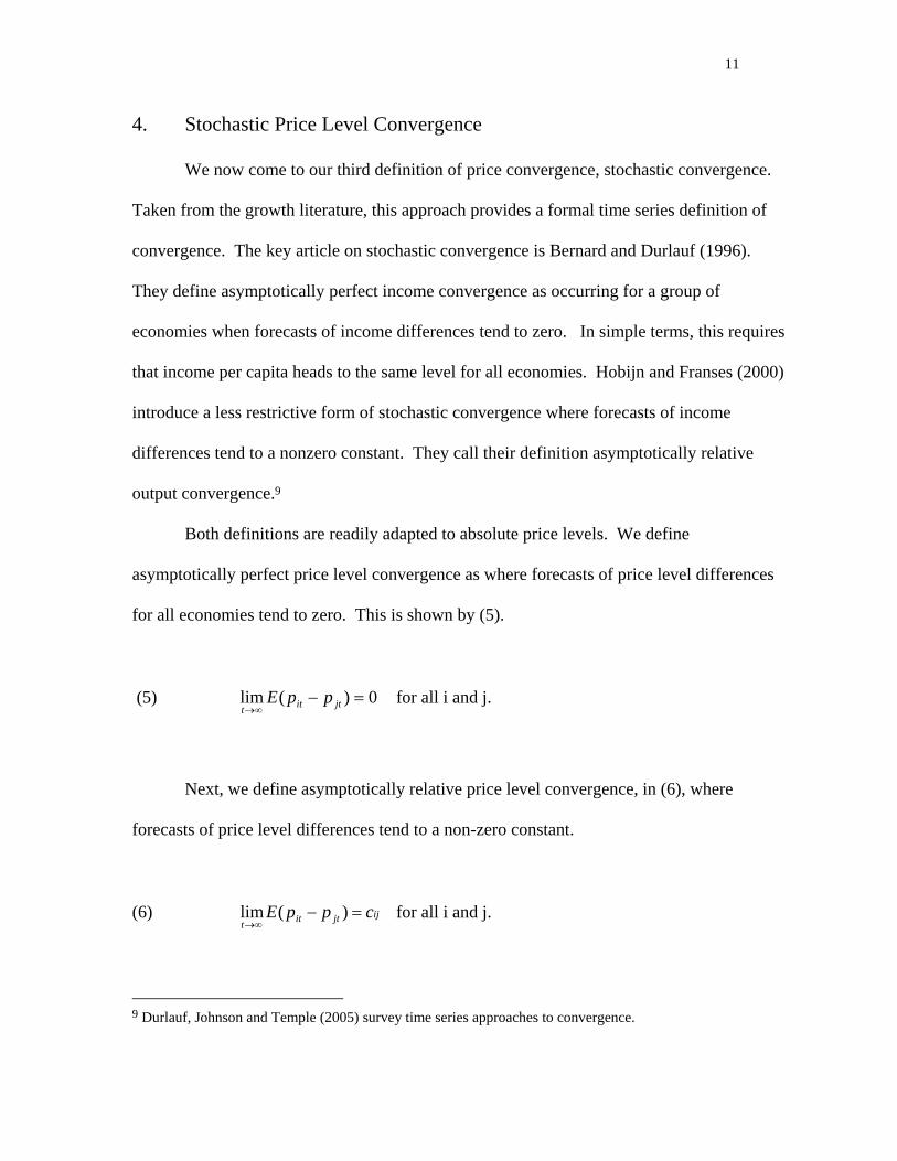
Both definitions are readily adapted to absolute price levels. We define

asymptotically perfect price level convergence as where forecasts of price level differences

for all economies tend to zero. This is shown by (5).

(5) for all i and j. 0)(lim =−∞→ jtitt

ppE

Next, we define asymptotically relative price level convergence, in (6), where

forecasts of price level differences tend to a non-zero constant.

(6) for all i and j. ijjtittcppE =−

∞→)(lim

9 Durlauf, Johnson and Temple (2005) survey time series approaches to convergence.

12

Stochastic convergence has a natural economic interpretation in terms of purchasing

power parity. From (5) we see that asymptotically perfect price level convergence equals

absolute purchasing power parity while relative price level convergence equals relative

purchasing power parity.

Before testing stochastic convergence we should first underline the fact that sigma

and stochastic convergence are fundamentally different concepts. Stochastic convergence

requires that price level differences are constant over time. In other words, it implies that

price level differences are stationary. With sigma convergence, however, price level

differences fall over time and are thus nonstationary.

Testing for Stochastic Convergence

Augmented Dickey-Fuller tests suggest that the absolute dollar price indices are of

integrated order one.10 Given a finding of nonstationarity, there are two ways to test

stochastic convergence. The first option is to test stochastic convergence using the

cointegration model of Bernard and Durlauf (1995, 1996). The second option is to test

bilateral level price differences for stationarity. We use the Bernard and Durlauf approach

because, unlike stationarity tests, it does not require a base country. Second, their approach

allows us to test for “club convergence”.11

Given that there are eleven economies, stochastic convergence requires ten

cointegrating vectors and one common trend. We use Johansen’s (1988, 1991) cointegration

10 Standard stationarity tests have low power in many circumstances, see Taylor and Taylor (2004). Our long time spans increase the power of the tests, but they also increase the likelihood of structural breaks due to changes in policy regime etc,. The tests also have low power with nonlinearities. 11 The cointegration and club tests also may lack power, see Pesaran (2004).

13

approach to test this restriction. First, we assume that we can represent the price series with a

Vector Autoregressive (VAR) process with constant terms. Next, we use the Akaike criteria

and Box-Pierce residual tests to determine the lag length of the process. The test results

indicate that the process has at most two lags in log prices with no serial correlation in

residual terms. In response, we chose two-year lags in log prices for the VAR. Using its

equivalent Vector Error Correction model form, we then test for cointegration based on the

trace and λmax test statistics. Table 2 provides the results.

[Insert Table 2 around here]

The first column is the number of cointegrating vectors, r. The second column is the

number of common trends m = n-r where n = number of series (11 countries). The null

hypothesis that r = 0 versus r > 0 is rejected by the trace and λmax test statistics at the 5%

significance level. As shown in the third row from the bottom, the λmax test rejects the null

that r = 2 but not r = 3. Using the trace test, the maximum number of cointergrating vectors

is four because the trace test rejects the null that r = 3 but not the null that r = 4 at the five

percent level. We conclude that there are, at most, four cointegrating relationships with

seven common trends suggesting. Thus, while price levels move together over the long run

stochastic convergence does not hold.

Next, we consider the possibility that stochastic convergence may hold for groups of

economies. We call this “club price convergence” as it corresponds to club convergence for

output. Club convergence occurs where asymptotically relative or absolute price level

convergence holds for a sub-group or club of economies. In the limit, a club could consist of

14

ten of the eleven economies. Thus, club convergence tells us if the rejection of stochastic

convergence is caused by one or a few economies.

To test for convergence clubs, we rely Hobijn and Franses (2000). Formal details

along with the results are in Appendix 2. As it turns out, the club tests show many small

clubs suggesting wide differences in price behavior across these economies. For absolute

price convergence, we find five to seven clubs. We also find five to seven clubs under

relative price convergence. In addition, the country groupings generated by the Hobijn and

Franses method are hard to justify on a priori grounds, as they are not grouped by a

geographical or cultural basis. In sum, our results reject stochastic convergence for the

overall sample and for economically meaningful sub-samples or clubs.12

5. A Cross Check

How robust are our findings? In particular, how robust is the finding that price levels

have converged less than income? This section cross checks the results with alternative price

level estimates based on GDP comparisons in current prices. In general, long run GDP

comparisons are formed in two ways. The first, followed by Maddison, is to project a single

benchmark comparison over time with domestic GDP series. As we have seen, this produces

a chained series in 1990 prices. The second approach, as in the early versions of the Penn

Tables, combines several benchmark income comparisons with times series from national 12 As mentioned, a problem with long span series is that structural breaks can bias the results of the cointegration tests. To investigate this possibility we used the Bai and Perron (2003a, 2003b) test that detects multiple structural breaks occurring at unknown dates. To test for structural change, we express each price level relative to the average price level of all other economies. The results show structural change for eight of the eleven economies. As it turns out, the breaks reduce the dispersion of price levels in a fashion consistent with Figure 2. They reinforce the conclusion that price level differences across economies are not constant, contrary to the predictions of stochastic convergence. The results and procedures are available from the authors.

15

accounts to form a GDP series that compares income in current prices.13 The question of

how to compare income over time stirred heated debates during the early stages of the Penn

Tables. The advantage of Maddison’s approach is that his estimates retain the growth rates

given by each country’s national accounts. In contrast, the second approach produces growth

rates that differ from the national accounts. As a result of the controversy, later versions of

the Penn Tables switched back to a single benchmark method.14 Bergin, Glick and Taylor

(2004) argue that the current price series still provide a useful cross check for results

obtained from the Maddison data.

Standard index number theory suggests that the absolute price deflators yielded by the

two approaches will differ in systematic ways. We can illustrate this point with a simple

example.15 Suppose we wish to compare income for a rich economy, country A, and a poor

economy, country B, for year T. We can compare income with prices from the rich economy

or with prices from the poor economy. A well-known result from the international

comparison literature shows that the rich economy prices yields generally lower income

differences as compared to using prices from the poorer economy (see Nuxoll (1994)).

Suppose now that we compare income for A and B using prices from a third economy,

economy C, that is richer than A or B. Nuxoll (1994) shows that in most circumstances this

will lead to even smaller income differences between A and B. Nuxoll’s results apply to

Maddison’s long run income comparisons because comparing income with chained 1990

13 A third approach, from the economic history literature, supplies benchmarks for individual years without providing annual series, see Prados de la Escosura (2000) or Ward and Devereux (2002). 14 Kravis and Lipsey (1991) review the controversy. For a recent debate in economic history over similar issues, see Broadberry (2003) and Ward and Devereux (2004). 15 Here we draw on the burgeoning literature on the Penn Tables. This work includes Nuxoll (1994), Dowrick and Quiggen (1997), Neary (2004) and Dowrick and Akmal (2005)

16

prices for past periods is equivalent to comparing income with prices from an economy that

is richer than the economies compared.16 This implies that Maddison’s estimates will tend to

understate income differences in the past relative to current prices. It also implies that they

will overstate price level dispersion.

Are these theoretical predictions borne out in the data? As it happens, Ward and

Devereux (2002) provide historical current price benchmarks for 1872, 1884, 1905, 1930 and

1950.17 Using their estimates, we find that price level dispersion in current prices for each

benchmark year is indeed lower than that from the Maddison price level deflators.

Do our results with respect to price level convergence hold with the current price

estimates? Unfortunately, Ward and Devereux (2002) do not provide annual GDP series.

We construct an annual series by combining their historical price level benchmarks with

Maddison's long run implicit price deflators using the method proposed by Summers and

Heston (1988) to reconcile differences between benchmarks and projections in international

comparisons.18 In viewing the results, it should be borne in mind that the Ward and

Devereux (2002) deflators are tentative. It should also be borne in mind that the Summers

and Heston approach to combining benchmark GDP comparisons and times series data

remains controversial.

16 Nuxoll (1994) provides a formal proof. 17 The 1950 benchmarks use high quality data from Gilbert and Kravis (1954, 1958). The 1905 and 1930 benchmarks use well-known contemporary price surveys while the 1872 and 1884 benchmarks use new sources, see Ward and Devereux (2002) for further details. The Ward and Devereux benchmarks use Fisher Ideal price indices since Geary Khamis measures are not available. 18 Summers and Heston (1978) combine benchmarks and times series by making assumptions about the reliability of the benchmarks relative to the long run projecting GDP series. We take the special case where benchmarks are measured without error. We then generate the current price series by minimizing the squared difference between the Maddison and the current price series subject to the constraint that current price series equal the benchmarks. This procedure will bias the results against Maddison. The more general case is where the benchmark and the Maddison estimates contain error.

17

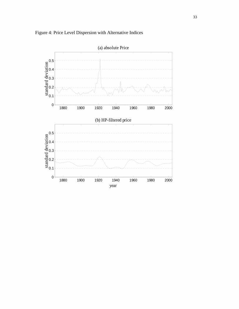
Figure 4 below provides absolute price level dispersion calculated from current series

with Panel (a) for raw price indices and Panel (b) for HP-filtered price indices. With the

exception of the Gold Standard, the current price series show no price level convergence.19

As mentioned, these results should be interpreted with care given that historical price level

benchmarks are in their infancy. Nevertheless, they underline the fact that long run income

comparisons depend on the base year used to compare income and price levels. The

alternative series strengthen our results in one crucial respect. They reinforce our previous

finding that convergence is more pronounced for output than prices.

[Insert Figure 4 around here]

19 The reduction in price level dispersion before 1914 in Figure 4 is consistent with the work of O’Rourke and Williamson (1999) that emphasizes the convergence of traded prices during the pre First World War era. The Maddison deflators show no such convergence.

18

6. Summing Up

Research in trade and growth has recently returned to the question of what determines

absolute price levels. This paper argues that the implicit deflators from the GDP volume

indices of Angus Maddison (1995, 2001 and 2003) provide a rich data set for the study of

long run absolute price levels. Using the Maddison deflators, we consider sigma, beta and

stochastic price level convergence for eleven developed economies from 1870 to 2004. The

empirical results support sigma and beta convergence. We find, however, that price level

convergence occurs later and to a lesser extent than for income per capita.20 We find no

evidence for stochastic price level convergence or for club price convergence.

20 Our results hold for developed economies where income has converged. A preliminary investigation suggests that prices have not converged over the long run where income does not converge. Leandro Prados de la Escosura (2000) provides a series for nominal and real GDP for Argentina, Austria, Belgium, Finland, Greece, Japan, New Zealand, Portugal, Spain and Turkey at roughly ten-year intervals. We supplement his estimates with our eleven economies plus data for India, Taiwan and Korea for Asia and Brazil, Mexico and Venezuela for Latin America. In total, we have data for twenty-seven economies for 1900, 1913, 1929, 1938, 1950, 1960, 1970, 1975, 1980, 1985 and 1990. We find that neither income nor price have converged for this sample. Indeed, price dispersion appears to have increased after 1950. Thus price level convergence, like income convergence, is not a general feature of the long run data.

19

REFERENCES

Abramovitz, Moses, “Catching Up, Forging Ahead and Falling Behind,” Journal of Economic History 46:3 (1986), 385-406. Bai, Jushan, and Pierre Perron, “Computation and Analysis of Multiple Structural Change Models,” Journal of Applied Econometrics 18:1 (2003a), 1-22. Bai, Jushan, and Pierre Perron, “Additional Critical Values for Multiple Structural Change Tests,” The Econometrics Journal 6:1 (2003a), 72-78. Balassa, Bela, “The Purchasing Power Parity Doctrine,” Journal of Political Economy 72:6 (1964), 584-596. Baumol, William. J., “Productivity Growth, Convergence, and Welfare: What the Long-Run Data Show,” American Economic Review 76:5 (1986), 1072-1085. Bergin, Patrick, Glick, Reuben and Alan. M. Taylor “Productivity Tradability and the Long Run Price Puzzle,” (NBER Working Paper 10569: New York, 2004). Bernard, Andrew and Steven M. Durlauf, "Convergence in International Output," Journal of Applied Econometrics 10:2 (1995), 97-108. Bernard, Andrew and Steven M. Durlauf, "Interpreting Tests of the Convergence Hypothesis," Journal of Econometrics 71:1-2 (1996), 161-174. Bhagwati, Jagdish, “Why are Services Cheaper in Poorer Economies?,” Economic Journal 94: 2 (1984), 296-286. Broadberry, Stephen, "Relative Per Capita Income Levels in the United Kingdom and the US since 1870," Journal of Economic History 63:3 (2003), 852-863. Durlauf, Steven, Johnson, Paul and Jonathan Temple “Growth Econometrics” in Phillippe. Aghion and Steven M. Durlauf (eds) The Handbook of Economic Growth (North Holland:Amsterdam 2005) DeLong, J. Bradford, “Productivity Growth, Convergence, and Welfare: Comment,” American Economic Review 78:5 (1988), 1138-54. Dowrick, Steven, and Muhammad Akmal, “Contradictory Trends in Global Income Inequality: A Tale of Two Biases,” Review of Income and Wealth 51:2 (2005), 201-229. Dowrick, Steven, and John Quiggen, “True Measures of GDP and Convergence,” American Economic Review 87:1 (1997), 41-64.

20

Friedman, Milton, “Prices of Money and Goods across Frontiers: The Pound and Dollar over a Century,” The World Economy 4:1 (1980), 497-511. Friedman, Milton, and Anna Schwartz, Monetary Trends in the United States and the United Kingdom: Their Relation to Income, Prices and Interest Rates, 1867-1965 (National Bureau of Economic Research: New York, 1982) Gilbert, Milton, and Irving Kravis, An International Comparison of National Products and the Purchasing Power of Currencies (OEEC: Paris, 1954). Gilbert, Milton, and Irving Kravis, Comparative National Products and Price Levels (OEEC: Paris, 1958). Hodrick, Robert and Edward Prescott, "Postwar US Business Cycles: An Empirical Investigation," Journal of Money Credit and Banking 29:1 (1997), 1-15. Hobijn, Bart, and Philip Franses, "Asymptotically Perfect and Relative Convergence of Productivity," Journal of Applied Econometrics 15:1 (2000), 59-81. Johansen Soren, and Katrina Juselius, “Statistical Analyses of Cointegration Vectors,” Journal of Economic Dynamics and Control 12:2-3 (1988), 231-254. Johansen Soren, and Katrina Juselius, “Estimation and Hypothesis Testing of Cointegration Vectors in Gaussian Autoregressive Models,” Econometrica 59:6 (1991), 1551-1580. Jones, Mathew T and Maurice Obstfeld “Savings, Investment and Gold: A Re-assessment of Historical Current Account Data,” (NBER Working Paper 6103: New York, 1997). Kravis, Irving and Robert Lipsey, “The International Comparison Program: Current Status and Problems,” in International Economic Transactions: Issues in Measurement and Empirical Research Peter Hooper and J. David Richardson, eds, (University of Chicago Press: Chicago 1991). Kwiatkowski, Denis, Phillips, Peter C. B., Schmidt, Peter and Yongcheol Shin, “Testing the Null Hypotheses of Stationarity against the Alternative of a Unit Root,” Journal of Econometrics 54:1-3 (1992), 159-178. Lee, Moon H., Purchasing Power Parity, (Marcel Dekker: New York, 1976). Maddison, Angus, “A Long Run Perspective on Saving,” Scandinavian Journal of Economics 94:2 (1992), 181-96. Maddison, Angus, Monitoring the World Economy 1820-1992 (Development Center of the Organization for Economic Co-Operation and Development: Paris, 1995).

21

Maddison, Angus, The World Economy: A Millennial Perspective (Development Center of the Organization for Economic Co-Operation and Development: Paris, 2001). Maddison, Angus, The World Economy: Historical Statistics (Development Center of the Organization for Economic Co-Operation and Development: Paris, 2003). Mitchell, Brian R, International Historical Statistics: Europe, 1750-2000 (Palgrave MacMillan: New York, 2004). Neary, J. Peter, "Rationalizing the Penn World Table: True Multilateral Indices for International Comparisons of Real Income," American Economic Review, 94: 5 (2004), 1411-1428. Norges Bank, Historical Statistics (Norges Bank Occasional Papers no 35: Oslo, 2004). Nuxoll, Daniel, “Differences in Relative Prices and International Differences in Growth Rates,” American Economic Review 84:5 (1994), 1423-1436. Obstfeld, Maurice and Alan M. Taylor, Global Capital Markets: Integration, Crisis, and Growth (Cambridge University Press: Cambridge, 2004). Ohlin, Bertil, Interregional and International Trade (Harvard University Press: Cambridge, 1933). O’Rourke, Kevin and Jeffrey Williamson Globalization and History: the Evolution of a Nineteenth-Century Atlantic Economy (MIT Press: Cambridge, 1999). Pesaran, M. Hashem, “A Pairwise Approach to Testing for Output and Growth Convergence,” (Unpublished, Cambridge University: Cambridge, 2004). Prados de la Escosura, Leandro, “International Comparisons of Real Product, 1820–1990: An Alternative Data Set,” Explorations in Economic History 37:1 (2000), 1-41. Sala-I-Martin, Xavier, “The Classical Approach to Convergence Analysis,” The Economic Journal 106:4 (1996), 1019-1036. Samelson, Paul A, "Theoretical Notes on Trade Problems," This Journal 23:2 (1996), 145-154. Schneider, Jeurgen and Oscar Schwarzer et al, Wahrungen de Welt I: Europaische und Nordamerikanische Devisenkurse 1777-1914 (Franz Steiner Verlag: Stuttgart, 1991). Summers, Robert and Heston, Alan, “A new set of international comparisons of real product and price levels estimates for 130 countries, 1950-1985,” Review of Income and Wealth 34:1 (1988), 1-25.

22

Taylor, Alan and Mark Taylor, “The Purchasing Power Parity Debate,” Journal of Economic Perspectives 18: Fall (2004),135-158. Ward, Marianne and John Devereux, “New Evidence on Catch-up and Convergence,” (Unpublished, Loyola College: Baltimore, 2002). Ward, Marianne and John Devereux, "A Reply to Professor Broadberry," Journal of Economic History 64: 3 (2004), 879-891.

23

Appendix 1: Data Sources

(a) Real GDP

Real GDP in chained 1990 prices from Maddison (2003) are at

http://www.eco.rug.nl/~Maddison/ downloaded in October 2006. We change the estimates

from Geary Khamis to Fisher Ideal indices using Maddison (1995) Table C-7 from page

172. Data for 2004 are from UN national income accounts at

http://unstats.un.org/unsd/snaama/Introduction.asp.

(b) Nominal GDP

All estimates are GDP in current market prices. For 1870-1980, nominal GDP

estimates for Australia, Canada, France, Germany, Netherlands, the UK and the US are from

the Maddison’s data files for Maddison (1992) at http://www.eco.rug.nl/~Maddison/. For

Germany and France, we interpolated for missing nominal GDP during wartime using CPI

indices and volume GDP indices from Maddison. Data for 1980 to 2004 are from UN

national accounts.

Sources for other economies: Denmark: Before 1967, we use Jones and Obstfeld

(1997) and Mitchell (2004). After 1967, data is from Stat Denmark. Italy: Jones and

Obstfeld (1997) and Mitchell (2004). After 1970 data is from UN national income accounts.

Norway: All data are from Norges Bank (2004). We interpolated missing Norwegian

nominal GDP data during the Second World War using CPI indices and volume GDP

indices from Maddison. Data for Sweden, 1870-1991, are from Persson at

http://www.iies.su.se/~perssont/ while1992-2004 are from UN national Income Accounts.

24

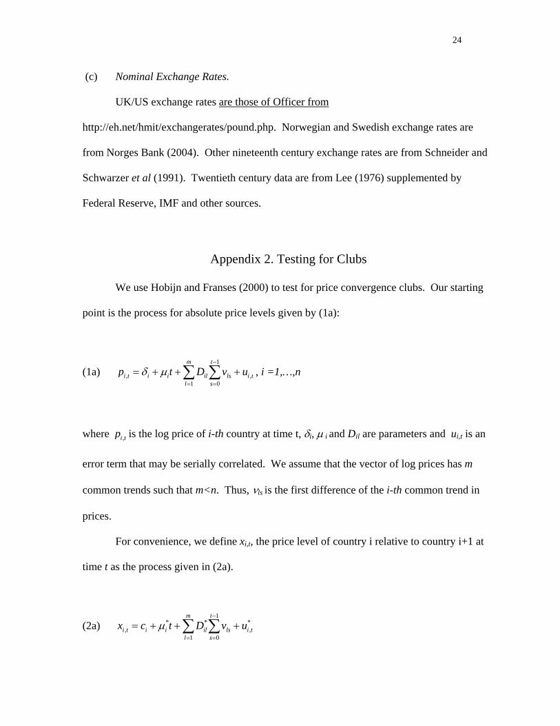
(c) Nominal Exchange Rates.

UK/US exchange rates are those of Officer from

http://eh.net/hmit/exchangerates/pound.php. Norwegian and Swedish exchange rates are

from Norges Bank (2004). Other nineteenth century exchange rates are from Schneider and

Schwarzer et al (1991). Twentieth century data are from Lee (1976) supplemented by

Federal Reserve, IMF and other sources.

Appendix 2. Testing for Clubs

We use Hobijn and Franses (2000) to test for price convergence clubs. Our starting

point is the process for absolute price levels given by (1a):

(1a) 1

, ,1 0

m t

i t i i il ls i tl s

p t D v uδ µ−

= =

= + + +∑ ∑ , i =1,…,n

where ,i tp is the log price of i-th country at time t, δi, µ i and Dil are parameters and ui,t is an

error term that may be serially correlated. We assume that the vector of log prices has m

common trends such that m<n. Thus, νls is the first difference of the i-th common trend in

prices.

For convenience, we define xi,t, the price level of country i relative to country i+1 at

time t as the process given in (2a).

(2a) 1

* *, ,

1 0

m t

i t i i il ls i tl s

*x c t D v uµ−

= =

= + + +∑ ∑

25

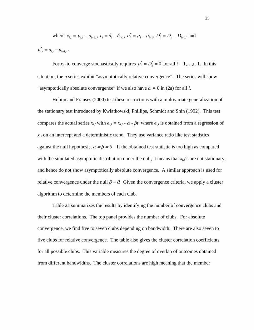
where * *, , 1, 1 1 1,, , , i t i t i t i i i i i i il il i lx p p c D D Dδ δ µ µ µ+ + += − = − = − = − +

1,

and

. *, ,i t i t i tu u u += −

For xi,t to converge stochastically requires * * 0i ilDµ = = for all i = 1,…,n-1. In this

situation, the n series exhibit “asymptotically relative convergence”. The series will show

“asymptotically absolute convergence” if we also have ci = 0 in (2a) for all i.

Hobijn and Franses (2000) test these restrictions with a multivariate generalization of

the stationary test introduced by Kwiatkowski, Phillips, Schmidt and Shin (1992). This test

compares the actual series xi,t with ei,t = xi,t - α - βt, where ei,t is obtained from a regression of

xi,t on an intercept and a deterministic trend. They use variance ratio like test statistics

against the null hypothesis, α = β = 0. If the obtained test statistic is too high as compared

with the simulated asymptotic distribution under the null, it means that xi,t’s are not stationary,

and hence do not show asymptotically absolute convergence. A similar approach is used for

relative convergence under the null β = 0. Given the convergence criteria, we apply a cluster

algorithm to determine the members of each club.

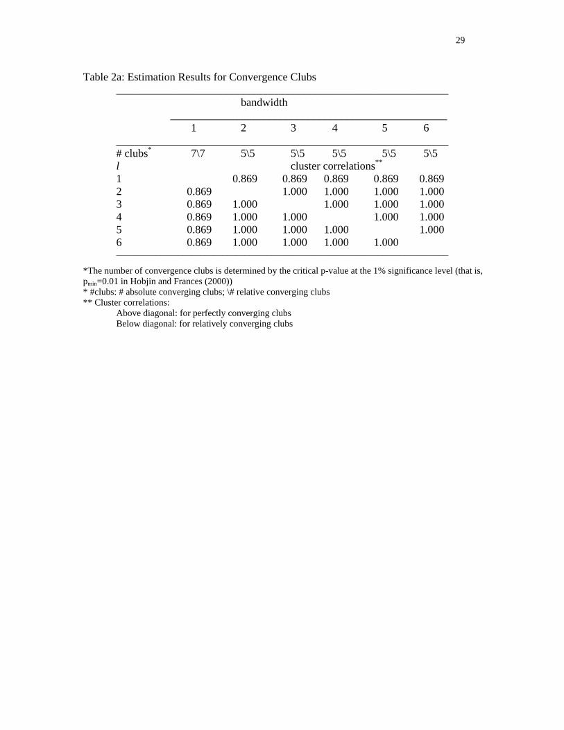
Table 2a summarizes the results by identifying the number of convergence clubs and

their cluster correlations. The top panel provides the number of clubs. For absolute

convergence, we find five to seven clubs depending on bandwidth. There are also seven to

five clubs for relative convergence. The table also gives the cluster correlation coefficients

for all possible clubs. This variable measures the degree of overlap of outcomes obtained

from different bandwidths. The cluster correlations are high meaning that the member

26

countries in one club are unlikely to appear a different club when the bandwidth changes.21

Hence, the results are robust to the choice of bandwidth.

[Insert Table 2a around here]

21 See Hobijn and Franses (2000) for the formula for cluster correlation.

27

Table 1: β - Convergence Regression Results ___________________________________________________________ Sample Period β estimate R2

______________________________________________________________________ 1870 – 2004 -0.008 0.80 (0.001) 1870 – 1913 -0.004 0.08 (0.004) 1913 – 1950 -0.006 0.13 (0.005) 1950 – 2004 -0.022 0.83 (0.003) ____________________________________________________________________ Note: Numbers in parenthesis are the standard errors of the estimates.

28

Table 2: Testing for Cointegration _______________________________________________________________________

Critical Values Critical Values r m Trace ____________ λmax ____________ 90% 95% 90% 95%

_____________________________________________________________________________________ 10 1 0.20 2.69 3.76 0.20 2.69 3.76 9 2 7.48 13.32 15.41 7.28 12.07 14.07 8 3 19.72 26.79 29.68 2.23 18.60 20.97 7 4 34.22 43.95 47.21 14.51 24.73 27.07 6 5 54.84 64.84 68.52 20.62 30.90 33.46 5 6 82.57 89.48 94.16 27.73 36.76 39.37 4 7 121.48 118.50 124.24 38.91 42.32 45.28 3 8 171.28 150.53 156.00 49.80 48.33 51.42 2 9 237.29 186.39 192.89 66.01 53.98 57.12 1 10 316.31 225.85 233.13 79.01 59.62 62.81 0 11 455.04 269.96 277.71 138.73 65.38 68.83 _____________________________________________________________________________________ Note: We use one lag in log price difference and constant terms in the Vector Error Correction Model. The first column, r, and the second column, m, are the number of cointegrating vectors and common trends respectively. The third and sixth columns are the Trace and λmax test statistics. The remaining columns show the critical values at 90% and 95% confidence levels.

29

Table 2a: Estimation Results for Convergence Clubs ____________________________________________________________ bandwidth __________________________________________________ 1 2 3 4 5 6 ____________________________________________________________ # clubs* 7\7 5\5 5\5 5\5 5\5 5\5 l cluster correlations**

1 0.869 0.869 0.869 0.869 0.869 2 0.869 1.000 1.000 1.000 1.000 3 0.869 1.000 1.000 1.000 1.000 4 0.869 1.000 1.000 1.000 1.000 5 0.869 1.000 1.000 1.000 1.000 6 0.869 1.000 1.000 1.000 1.000 ___________________________________________________________________________ *The number of convergence clubs is determined by the critical p-value at the 1% significance level (that is, pmin=0.01 in Hobjin and Frances (2000)) * #clubs: # absolute converging clubs; \# relative converging clubs ** Cluster correlations: Above diagonal: for perfectly converging clubs Below diagonal: for relatively converging clubs

30

Figure 1: The Absolute Price Indices

1880 1900 1920 1940 1960 1980 20000.5

1

1.5

2

2.5

3

3.5

4

4.5

5

5.5AustraliaCanadaDenmarkFranceGermanyItalyNetherlandsNorwaySwedenUKUS

log

pric

e

year

31

Figure 2: Price and income dispersion 1870-2004

1880 1900 1920 1940 1960 1980 20000.1

0.2

0.3

0.4

0.5

0.6

(a) per capita incomest

anda

rd d

evia

tion

1880 1900 1920 1940 1960 1980 20000.1

0.2

0.3

0.4

0.5

0.6

(b) absolute price

stan

dard

dev

iatio

n

1880 1900 1920 1940 1960 1980 20000.1

0.2

0.3

0.4

0.5

0.6

(c) HP-filtered price

year

stan

dard

dev

iatio

n

32

Figure 3: Beta Price Level Convergence

2.2 2.4 2.6 2.8 30.03

0.035

0.04

0.045

0.05

0.055

0.06

log absolute price in 1950

log

abso

lute

pric

e ch

ange Italy

Netherlands

Germany UK

Denmark

Australia

Sweden

Norway

France

Canada

US

33

Figure 4: Price Level Dispersion with Alternative Indices

1880 1900 1920 1940 1960 1980 20000

0.1

0.2

0.3

0.4

0.5

stan

dard

dev

iatio

n(a) absolute Price

1880 1900 1920 1940 1960 1980 20000

0.1

0.2

0.3

0.4

0.5

(b) HP-filtered price

year

stan

dard

dev

iatio

n