hazards in choosing between pooled and separate- variances ... · hazards in choosing between...
TRANSCRIPT
Psicológica (2009), 30, 371-390.
Hazards in Choosing Between Pooled and Separate-
Variances t Tests
Donald W. Zimmerman1 & Bruno D. Zumbo
2
1Carleton University, Canada;
2University of British Columbia, Canada
If the variances of two treatment groups are heterogeneous and, at the same
time, sample sizes are unequal, the Type I error probabilities of the pooled-
variances Student t test are modified extensively. It is known that the
separate-variances tests introduced by Welch and others overcome this
problem in many cases and restore the probability to the nominal
significance level. In practice, however, it is not always apparent from
sample data whether or not the homogeneity assumption is valid at the
population level, and this uncertainty complicates the choice of an
appropriate significance test. The present study quantifies the extent to
which correct and incorrect decisions occur under various conditions.
Furthermore, in using statistical packages, such as SPSS, in which both
pooled-variances and separate-variances t tests are available, there is a
temptation to perform both versions and to reject H0 if either of the two test
statistics exceeds its critical value. The present simulations reveal that this
procedure leads to incorrect statistical decisions with high probability.
It is well known that the two-sample Student t test depends on an
assumption of equal variances in treatment groups, or homogeneity of
variance, as it is known. It is also recognized that violation of this
assumption is especially serious when sample sizes are unequal (Hsu, 1938;
Scheffe′, 1959, 1970). The t and F tests, which are robust under some
violations of assumptions (Boneau, 1960), are decidedly not robust when
heterogeneity of variance is combined with unequal sample sizes.
A spurious increase or decrease of Type I and Type II error
probabilities occurs when the variances of samples of different sizes are
pooled to obtain an error term. If the larger sample is taken from a
population with larger variance, then the pooled error term is inflated,
resulting in a smaller value of the t statistic and a depressed Type I error
1 Correspondence: Donald W. Zimmerman, Ph.D. Professor Emeritus of Psychology,
Carleton University. Ottawa, Canada. Mailing address: 1978 134A Street. Surrey, BC,
Canada, V4A 6B6. 2
Bruno D. Zumbo, Ph.D. Professor of Measurement and Statistics. University of British
Columbia. Vancouver, BC, Canada. Email: [email protected]
D.W. Zimmerman & B.D. Zumbo 372
probability. If the smaller sample is taken from a population with larger
variance, the reverse is true (Overall, Atlas, & Gibson, 1995a, 1995b). See
also the informative graphs presented by Hopkins, Glass, & Hopkins (1987,
p. 168).
In the literature, the need to modify the t test when the assumption of
equal variances is violated has been known as the Behrens-Fisher problem
(Behrens, 1929; Fisher, 1935). Early investigations showed that the problem
can be overcome by substituting separate-variances tests, such as the ones
introduced by Welch (1938, 1947), and Satterthwaite (1946), for the
Student t test, and similar methods are available for the ANOVA F test.
These modified significance tests, unlike the usual two-sample Student t
test, do not pool variances in computation of an error term. Moreover, they
alter the degrees of freedom by a function that depends on sample data. It
has been found that these procedures in many cases restore Type I error
probabilities to the nominal significance level and also counteract increases
or decreases of Type II error probabilities (see, for example, Overall, Atlas,
& Gibson, 1995a, 1995b; Zimmerman, 2004; Zimmerman & Zumbo, 1993).
In recent years, separate-variances t tests have become more widely used
and are included in various statistical software packages such as SPSS.
The purpose of this paper is to call attention to some unforeseen
dangers of this approach. For one thing, it is not easy to discern from
sample data whether or not the populations from which the samples are
drawn do in fact support or violate the homogeneity assumption. If a
decision as to which test to employ is based on anomalous sample data that
does not represent the population, the result can be misleading. Apparently
homogeneous samples can arise frequently from heterogeneous populations,
and vice versa. In those cases, choice of an inappropriate test can lead to a
wrong decision, and sampling variability may produce that outcome more
often than might be suspected.
Another difficulty arises because some researchers using software
packages, such as SPSS, may be inclined to employ both pooled-variances
and separate-variances tests when in doubt about the homogeneity
assumption and report the result of whichever version yields statistical
significance. The spurious increase in the probability of rejecting H0
resulting from applying multiple significance tests to the same data and then
picking and choosing the desired result is well established. However, the
problem is somewhat more serious and less apparent in the case of the two
versions of the t test, and incorrect statistical decisions, we shall see, can
occur with very high frequency when the two tests are performed together.
Pooled and separate-variances t-tests
373
The present study quantifies the extent of correct and incorrect
decisions that can be expected under various scenarios where sample data is
not representative of the population. It also examines the modifications of
significance levels that occur when a decision is based on the Student t test
alone, on the Welch t test alone, or on a favorable outcome of either test.
METHOD*
The simulations in this study were programmed using Mathematica,
version 4.1, together with Mathematica statistical add-on packages. Each
replication of the sampling procedure obtained two independent samples of
n1 and n2 scores. For successive pairs, all scores in one sample were
multiplied by a constant, so that the ratio σ1/σ2 had a predetermined value.
This ratio varied from 1.0 to 1.8 in increments of .1 and then from 2 to 3 in
increments of .5. In another part of the study, the ratio was 1.02, 1.05, 1.10,
and 1.15. In most cases the sample sizes n1 and n2 varied between 10 and
60, in such a way that the ratio n1/n2 was 1/6, 1/5, 1/4, 1/3, 1/2, 2/3, 3/2, 2,
3, 4, 5, or 6. The total sample size n1 + n2 was fixed at 60 for the data in
Tables 1 and 2 and in Figures 1, 2, and 3. There were 50,000 replications of
the sampling procedure for each condition in the study.
As a check, some simulations in Figures 1 and 2 in the study were
repeated using random numbers generated by the method of Marsaglia,
Zaman, & Tsang (1990), described by Pashley (1993), together with normal
deviates obtained by the procedure of Marsaglia & Bray (1964). These
methods reproduced the results in the tables very closely, so all subsequent
simulations employed random normal deviates obtained directly from the
Mathematica statistical add-on package.
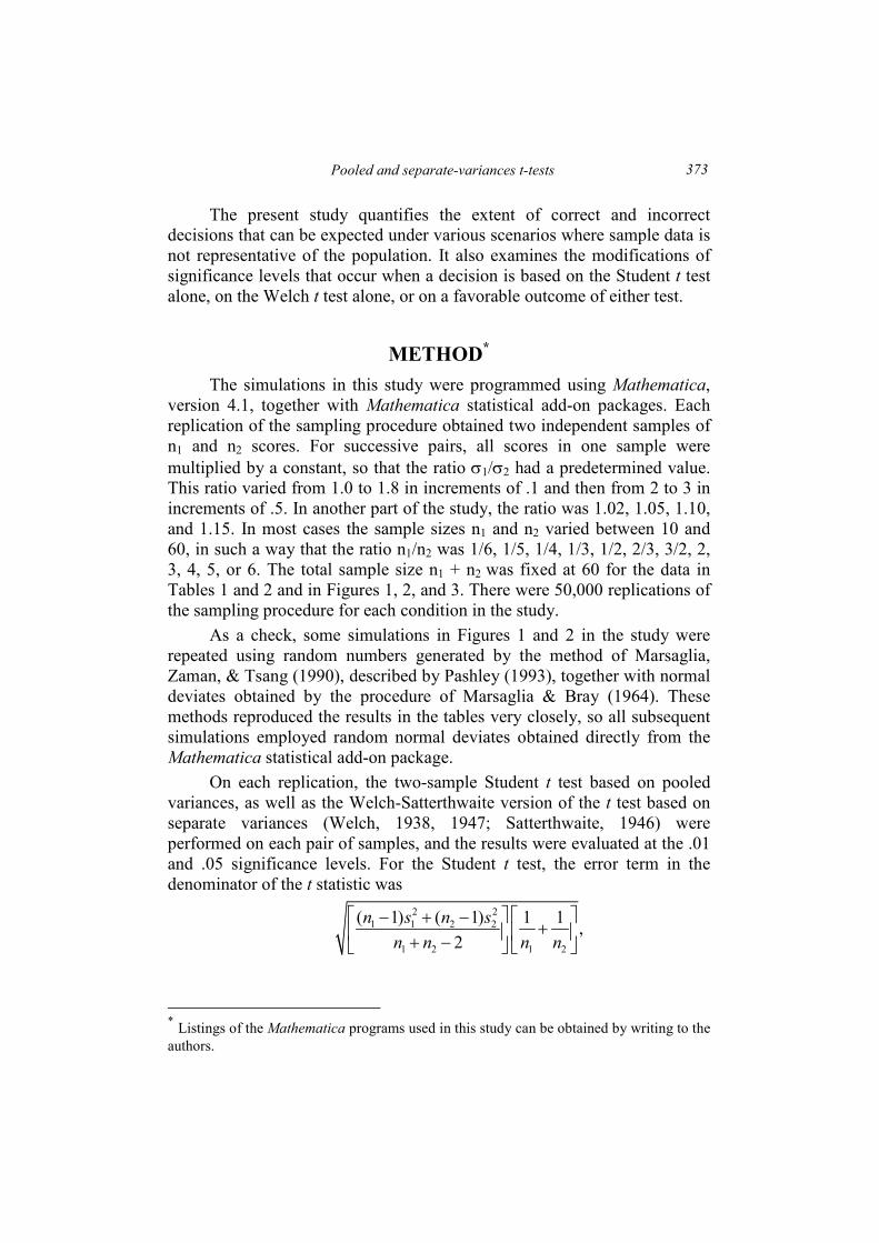
On each replication, the two-sample Student t test based on pooled
variances, as well as the Welch-Satterthwaite version of the t test based on
separate variances (Welch, 1938, 1947; Satterthwaite, 1946) were
performed on each pair of samples, and the results were evaluated at the .01
and .05 significance levels. For the Student t test, the error term in the
denominator of the t statistic was
2 2
1 1 2 2
1 2 1 2
( 1) ( 1) 1 1,
2
n s n s
n n n n
− + −+
+ −
* Listings of the Mathematica programs used in this study can be obtained by writing to the
authors.
D.W. Zimmerman & B.D. Zumbo 374
where n1 and n2 are sample sizes, and 2
1s and 2
2s are sample variances,
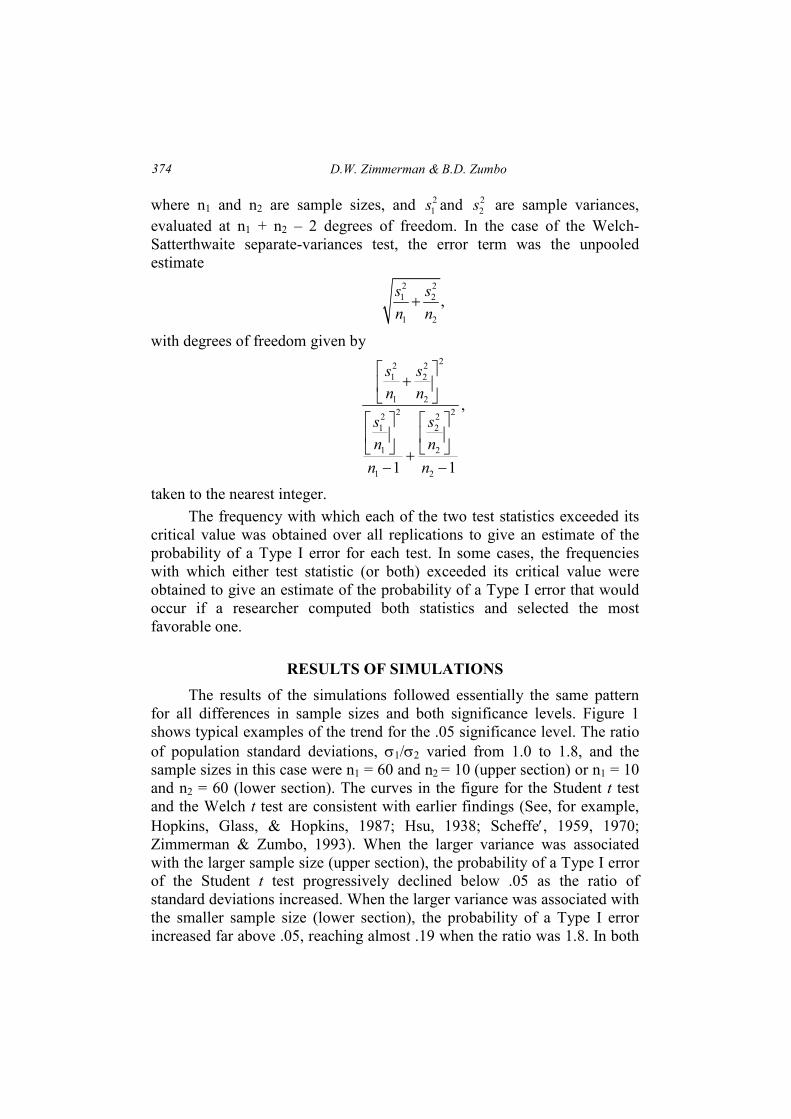
evaluated at n1 + n2 – 2 degrees of freedom. In the case of the Welch-
Satterthwaite separate-variances test, the error term was the unpooled
estimate
2 2
1 2
1 2
,s s
n n+
with degrees of freedom given by
22 2
1 2
1 2
2 22 2
1 2
1 2
1 2
,
1 1
s s
n n
s s
n n
n n
+
+− −
taken to the nearest integer.
The frequency with which each of the two test statistics exceeded its
critical value was obtained over all replications to give an estimate of the
probability of a Type I error for each test. In some cases, the frequencies
with which either test statistic (or both) exceeded its critical value were
obtained to give an estimate of the probability of a Type I error that would
occur if a researcher computed both statistics and selected the most
favorable one.
RESULTS OF SIMULATIO%S
The results of the simulations followed essentially the same pattern
for all differences in sample sizes and both significance levels. Figure 1
shows typical examples of the trend for the .05 significance level. The ratio
of population standard deviations, σ1/σ2 varied from 1.0 to 1.8, and the
sample sizes in this case were n1 = 60 and n2 = 10 (upper section) or n1 = 10
and n2 = 60 (lower section). The curves in the figure for the Student t test
and the Welch t test are consistent with earlier findings (See, for example,
Hopkins, Glass, & Hopkins, 1987; Hsu, 1938; Scheffe′, 1959, 1970;
Zimmerman & Zumbo, 1993). When the larger variance was associated
with the larger sample size (upper section), the probability of a Type I error
of the Student t test progressively declined below .05 as the ratio of
standard deviations increased. When the larger variance was associated with
the smaller sample size (lower section), the probability of a Type I error
increased far above .05, reaching almost .19 when the ratio was 1.8. In both
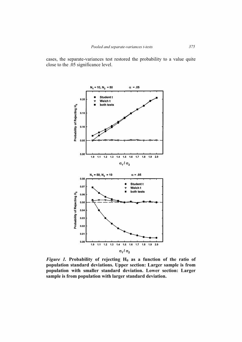
Pooled and separate-variances t-tests
375
cases, the separate-variances test restored the probability to a value quite
close to the .05 significance level.
Figure 1. Probability of rejecting H0 as a function of the ratio of
population standard deviations. Upper section: Larger sample is from
population with smaller standard deviation. Lower section: Larger
sample is from population with larger standard deviation.
D.W. Zimmerman & B.D. Zumbo 376
For the procedure in which the outcome of both tests determined the
decision, the probability of a Type I error again depended on whether the
larger variance was associated with the larger or smaller sample size. In the
former case, this probability spuriously increased above the .05 significance
level, although the probability for the Student t test alone declined below
.05.
In the case where the larger variance was associated with the smaller
sample size, the spurious increase in probability for the combination of both
tests exceeded the increase for the Student t test alone but became gradually
less as the ratio of standard deviations increased. Obviously, when the
larger variance is associated with the smaller sample size, using both the
pooled-variance test and the separate-variance test together and selecting
the most favorable outcome, does not restore the .05 significance level. In
fact, it makes the spurious increase in the probability of rejecting H0
somewhat worse than it is when using the Student t test alone. Again, the
change was greatest when the difference between the two standard
deviations was slight rather than extreme.
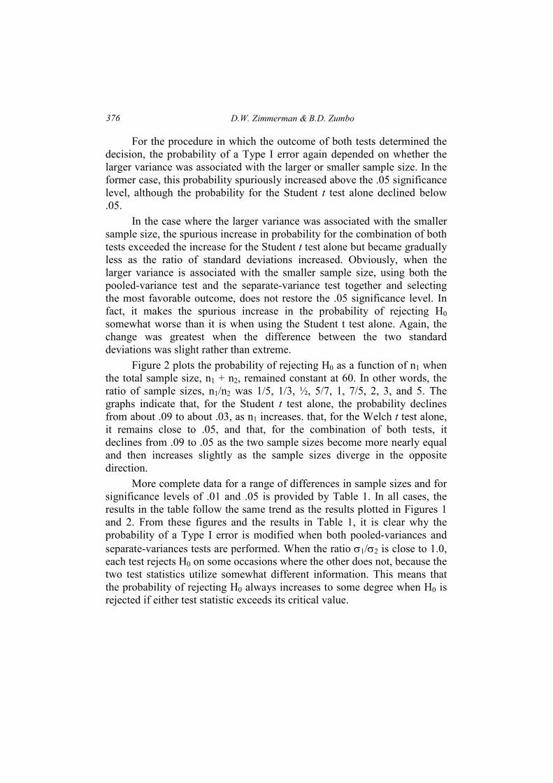
Figure 2 plots the probability of rejecting H0 as a function of n1 when
the total sample size, n1 + n2, remained constant at 60. In other words, the
ratio of sample sizes, n1/n2 was 1/5, 1/3, ½, 5/7, 1, 7/5, 2, 3, and 5. The
graphs indicate that, for the Student t test alone, the probability declines
from about .09 to about .03, as n1 increases. that, for the Welch t test alone,
it remains close to .05, and that, for the combination of both tests, it
declines from .09 to .05 as the two sample sizes become more nearly equal
and then increases slightly as the sample sizes diverge in the opposite
direction.
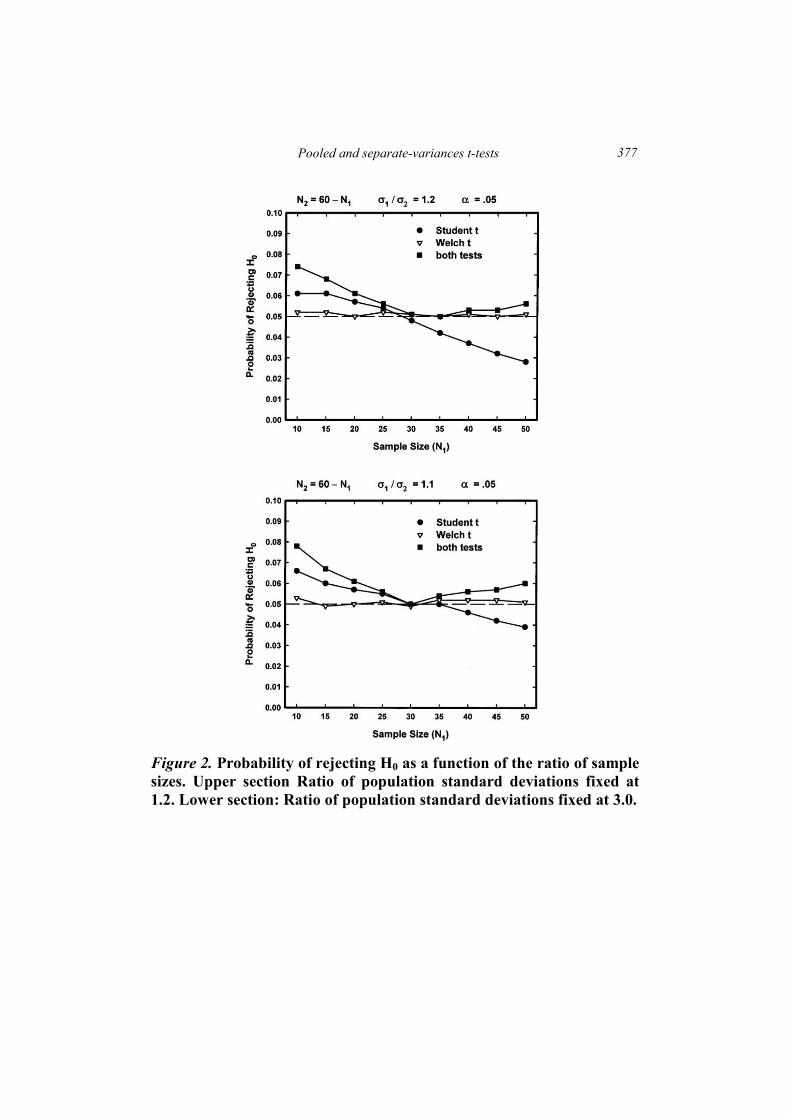
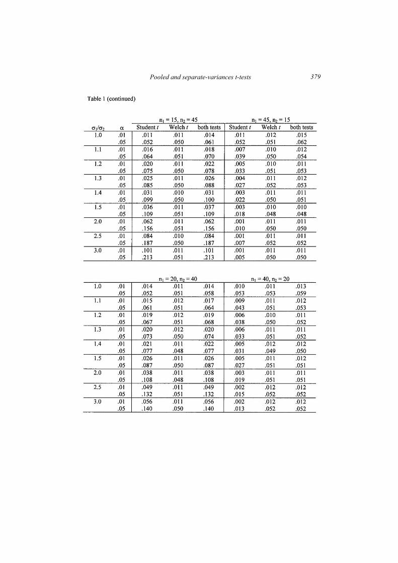
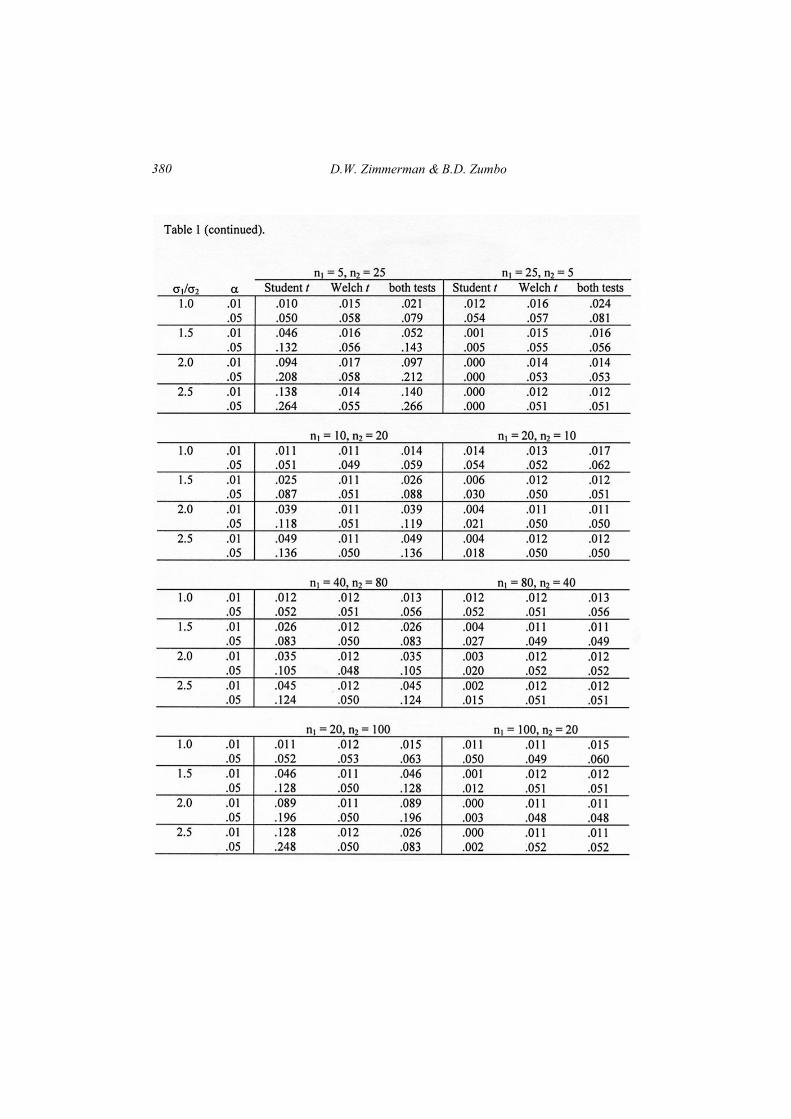
More complete data for a range of differences in sample sizes and for
significance levels of .01 and .05 is provided by Table 1. In all cases, the
results in the table follow the same trend as the results plotted in Figures 1
and 2. From these figures and the results in Table 1, it is clear why the
probability of a Type I error is modified when both pooled-variances and
separate-variances tests are performed. When the ratio σ1/σ2 is close to 1.0,
each test rejects H0 on some occasions where the other does not, because the
two test statistics utilize somewhat different information. This means that
the probability of rejecting H0 always increases to some degree when H0 is
rejected if either test statistic exceeds its critical value.
Pooled and separate-variances t-tests
377
Figure 2. Probability of rejecting H0 as a function of the ratio of sample
sizes. Upper section Ratio of population standard deviations fixed at
1.2. Lower section: Ratio of population standard deviations fixed at 3.0.
D.W. Zimmerman & B.D. Zumbo 378
Pooled and separate-variances t-tests
379
D.W. Zimmerman & B.D. Zumbo 380
Pooled and separate-variances t-tests
381
On the other hand, when the ratio σ1/σ2 is more extreme, one test
dominates, depending on whether the larger variance is associated with the
larger or smaller sample size. In the former case, the Welch test exceeds its
critical value with probability close to .05, and there are relatively few cases
where the Student t statistic exceeds its critical value and the Welch statistic
does not. Substantial increases above .05 are limited to values of the ratio
not too far from 1.0, for which each test rejects H0 on a considerable
number of occasions. However, when the larger variance is associated with
the smaller sample size, there are substantial increases in probability of
rejecting H0 over the entire range of the ratio σ1/σ2. Unfortunately, reaching
a decision by considering both test statistics eliminates the improvement
that results from using the Welch test alone.
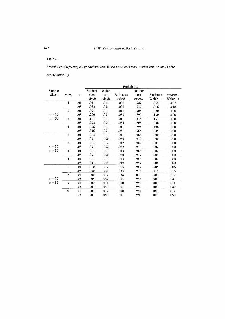
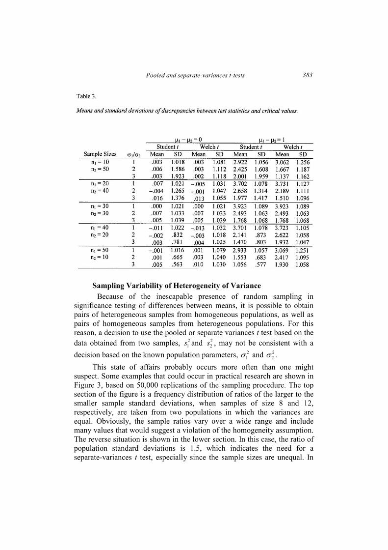
Table 2 presents a breakdown of the total number of sampling
occasions into instances where both tests resulted in the same statistical
decision, either rejection or no rejection, as well as instances where the two
tests resulted in different decisions, either rejection by the Student t test and
no rejection by the Welch test, or vice versa. Also shown are the overall
probabilities of rejection by each significance test. The sum of the values in
the last 4 columns always is 1.0, within the limits of rounding error. Also,
the value in the column labeled “Student t test rejects” is the sum of the
value in the column labeled “Both tests reject” and the value in the column
labeled “Student +, Welch −.” Similarly, the value in the column labeled
“Welch test rejects” is the sum of the value in the column labeled “Both
tests reject” and the value in the column labeled “Student − , Welch +.”
When sample sizes are equal, there are relatively few occasions on
which one test rejects H0 and the other does not. Both tests reject H0 with
probability close to the nominal significance level, irrespective of equality
or inequality of population variances. The same is true when population
variances are equal but sample sizes are not. When both population
variances and sample sizes are unequal and the smaller sample size is
associated with the larger variance, there are no occasions on which the
Welch test rejects and the Student t test does not. When both variances and
sample sizes are unequal and the larger sample size is associated with the
larger variance, the outcome is the reverse: There are no occasions on which
the Student t test rejects and the Welch test does not. In other words,
extensive inflation or depression of the probability of rejection of H0 by the
Student t test is associated with a difference in the outcomes of the
respective tests. The two tests are almost but not quite completely consistent
when sample sizes are equal or when population variances are equal.
D.W. Zimmerman & B.D. Zumbo 382
Pooled and separate-variances t-tests
383
Sampling Variability of Heterogeneity of Variance
Because of the inescapable presence of random sampling in
significance testing of differences between means, it is possible to obtain
pairs of heterogeneous samples from homogeneous populations, as well as
pairs of homogeneous samples from heterogeneous populations. For this
reason, a decision to use the pooled or separate variances t test based on the
data obtained from two samples, 2
1s and 2
2s , may not be consistent with a
decision based on the known population parameters, 2
1σ and 2
2σ .
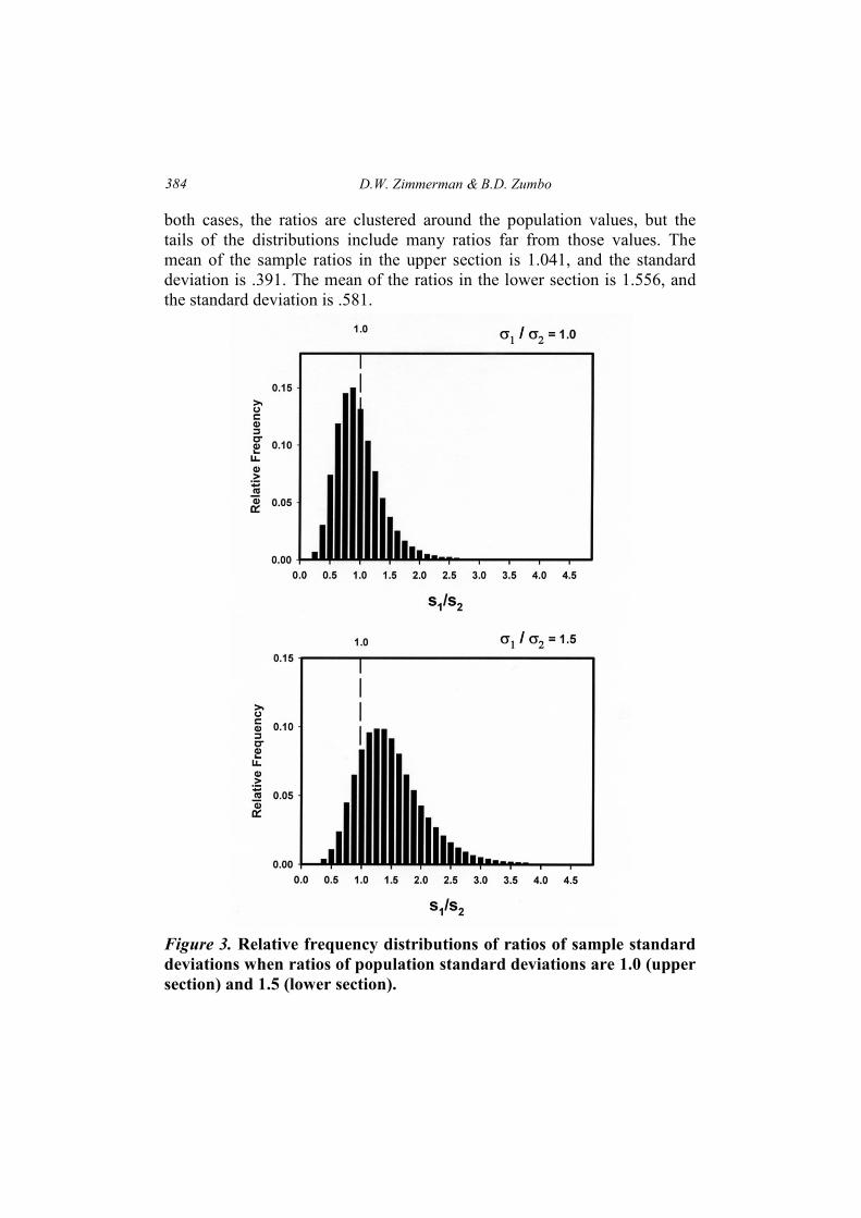
This state of affairs probably occurs more often than one might
suspect. Some examples that could occur in practical research are shown in
Figure 3, based on 50,000 replications of the sampling procedure. The top
section of the figure is a frequency distribution of ratios of the larger to the
smaller sample standard deviations, when samples of size 8 and 12,
respectively, are taken from two populations in which the variances are
equal. Obviously, the sample ratios vary over a wide range and include
many values that would suggest a violation of the homogeneity assumption.
The reverse situation is shown in the lower section. In this case, the ratio of
population standard deviations is 1.5, which indicates the need for a
separate-variances t test, especially since the sample sizes are unequal. In
D.W. Zimmerman & B.D. Zumbo 384
both cases, the ratios are clustered around the population values, but the
tails of the distributions include many ratios far from those values. The
mean of the sample ratios in the upper section is 1.041, and the standard
deviation is .391. The mean of the ratios in the lower section is 1.556, and
the standard deviation is .581.
Figure 3. Relative frequency distributions of ratios of sample standard
deviations when ratios of population standard deviations are 1.0 (upper
section) and 1.5 (lower section).
Pooled and separate-variances t-tests
385
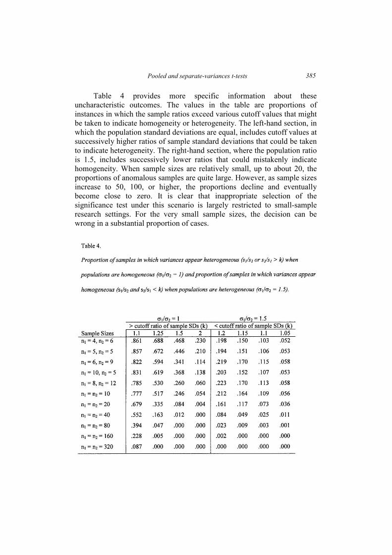
Table 4 provides more specific information about these
uncharacteristic outcomes. The values in the table are proportions of
instances in which the sample ratios exceed various cutoff values that might
be taken to indicate homogeneity or heterogeneity. The left-hand section, in
which the population standard deviations are equal, includes cutoff values at
successively higher ratios of sample standard deviations that could be taken
to indicate heterogeneity. The right-hand section, where the population ratio
is 1.5, includes successively lower ratios that could mistakenly indicate
homogeneity. When sample sizes are relatively small, up to about 20, the
proportions of anomalous samples are quite large. However, as sample sizes
increase to 50, 100, or higher, the proportions decline and eventually
become close to zero. It is clear that inappropriate selection of the
significance test under this scenario is largely restricted to small-sample
research settings. For the very small sample sizes, the decision can be
wrong in a substantial proportion of cases.
D.W. Zimmerman & B.D. Zumbo 386
Effects of Slight Variance Heterogeneity Together with Unequal
Sample Sizes
The probability of rejecting H0 by the Student t test is severely
inflated or depressed when sample sizes are unequal at the same time
variances are heterogeneous. If one of the two is not an issue─ that is, if
variances are equal or if sample sizes are the same─the influence of the
other is not large. However, when both conditions occur at the same time,
the influence of one can be greatly magnified by changes in the other.
Table 5 exhibits some cases where ratios of population standard
deviations fairly close to 1.0 produce large changes in the probability of
rejecting H0 provided sample sizes differ greatly. For example, a ratio of
standard deviations of only 1.05 elevates or depresses the probability of
rejecting H0 considerably above or below the nominal significance level
when the difference in sample sizes is large, such as n1 = 10 and n2 = 100.
Even a ratio of only 1.02 has noticeable effects under these large differences
in sample sizes. The data in Table 5 also show that the Welch test still
restores the probability to a value fairly close to the nominal significance
level in these extreme cases.
Considering the results in Table 5 together with the results of
sampling variability shown in the foregoing tables, it becomes clear that
there is a danger in disregarding slight differences in sample variances and
assuming that the Student t test is appropriate, especially if the difference in
sample sizes is large. The slight differences in standard deviations included
in Table 5, we have seen, can be expected to arise frequently from sampling
variability even though population variances are equal. In such instances, a
large difference in sample sizes can lead to an incorrect statistical decision
by the Student t test with high probability
FURTHER DISCUSSIO%
If multiple significance tests are performed on the same data at the
same significance level, and if H0 is rejected when any one of the various
test statistics exceeds its critical value, the probabilities of Type I and Type
II errors are certainly modified to some extent. For example, if a Student t
test and a Wilcoxon-Mann-Whitney test are performed on the same data, at
the .05 significance level, then this omnibus procedure makes the Type I
error probability about .055, or perhaps .06. For other significance tests of
differences between means, the outcome is about the same. In the case of
most commonly used significance tests of location, the change is not large,
and textbooks pay relatively little attention to this illegitimate procedure.

Pooled and separate-variances t-tests
387
The result is always an increase in Type I error probability, because the
critical region for multiple tests is a union of the critical regions of the
individual tests. Since various significance tests utilize much the same
information in the data, the change usually is minimal.

D.W. Zimmerman & B.D. Zumbo 388
However, in the case of the pooled-variances and separate-variances t
tests, the outcome of such a procedure is quite different and more serious.
The disparity arises as a consequence of two effects of heterogeneous
variances. First, the probability of a Type I error is altered extensively when
the ratio of variances and the ratio of sample sizes are both large. Second,
the direction of the change depends on whether the larger variance is
associated with the larger or smaller sample size. In the first case the
probability of a Type I error declines below the nominal significance level,
and in the second case it increases (see Figure 1 and Table 1).
Suppose, for example, that the ratio σ1/σ2 is about 1.1, that n1 = 60, n2
= 10, and that both pooled-variances and separate-variances tests are
performed at the .05 significance level. Then, it is clear from Figure 1 that
rejecting H0 when either test statistic exceeds its critical value makes the
probability of a Type I error about .06 instead of .05. This can be contrasted
with the decline to .035 when the pooled-variances test alone is performed.
However, the probability for the separate-variances test alone is close to
.05.
Next, suppose the ratio σ1/σ2 remains 1.1, while the sample sizes are
reversed: n1 = 10 and n2 = 60. Then, rejecting H0 when either test statistic
exceeds its critical value makes the probability of a Type I error about .08,
which is worse than the .07 resulting from the pooled-variances test alone.
Again, the separate-variances test alone yields the correct value of .05. If
the ratio σ1/σ2 is somewhat larger, say, 1.6, then performing both tests
makes the probability of a Type I error about .15, which is the same as
employing the pooled-variances test alone. In this case, rejecting H0 after
applying the separate-variances test alone has a more favorable outcome.
The result of performing both pooled-variances and separate-
variances tests on the same data, therefore, is not simply an increase in the
probability of rejecting H0 to a value slightly above the nominal
significance level, because of capitalizing on chance. That is true only if the
ratio σ1/σ2 falls in a rather narrow range between about 1.0 and about 1.5
and, in addition, the larger sample is associated with the larger variance. In
all cases of heterogeneous variances examined in the present study,
employing the separate-variance test alone resulted in rejecting H0 with
probability close to the nominal significance level. In most cases, the
pooled-variances test, either alone or in combination with the separate-
variances test, substantially altered the probability. To look at it another
way, reaching a decision by considering both the pooled and separate-
variances test statistics together eliminates the improvement that comes
from using the separate-variances test alone.
Pooled and separate-variances t-tests
389
Another complication arises from the fact that researchers may not
always know when population variances are heterogeneous. And in some
cases it is even problematic whether a larger variance is associated with a
larger or smaller sample size. If the ratio of sample sizes is quite different
from 1.0, say 1/4 or 1/5, then the probability of a Type I error is sensitive to
slight differences in population variability. For example, as we have seen,
an apparently inconsequential ratio of standard deviations of 1.1 can
increase the probability of a Type I error substantially. On the other hand,
interchanging the larger and smaller standard deviations, so that the ratio
becomes .91, significantly decreases the nominal Type I error probability.
Because sample variances do not always reflect population variances,
it is difficult to determine whether Type I error probabilities will increase or
decrease if sample sizes differ. A ratio of sample standard deviations of 1.1
or 1.2 could easily arise in sampling from populations with ratios
considerably more extreme and possibly when the ratio is less than 1.0. The
sensitivity of the Type I error probabilities to small differences, makes it
risky to reach a decision about the appropriate test solely on the basis of
sample statistics.
Preliminary tests of equality of variances, such as the Levene test, the
F test, or the O’Brien test, are ineffective and actually make the situation
worse (Zimmerman, 2004). That is true because, no matter what
preliminary test is chosen, it inevitably produces some Type II errors. On
those occasions, therefore, a pooled- variances test is performed when a
separate-variances test is needed, modifying the significance level to some
degree. On the other hand, a Type I error, resulting in using a separate-
variances test when variances are actually homogeneous, is of no
consequence.
Instead of inspecting sample data and performing a preliminary test of
homogeneity of variance, it is recommended that researchers focus attention
on sample sizes. Then, to protect against possible heterogeneity of variance,
simply perform a separate-variances test unconditionally whenever sample
sizes are unequal. That strategy protects the significance level if population
variances are unequal, whatever the outcome of a preliminary test might be.
And if variances are in fact homogeneous, nothing is lost, because then both
pooled and separate-variances tests lead to the same statistical decision.

D.W. Zimmerman & B.D. Zumbo 390
REFERE%CES
Behrens, W.U. (1929). Ein Beitrag zur Fehlerberechnung bei wenigen Beobachtungen.
Landwirtschaftlisches Jahrbuch, 68, 807-837.
Boneau, C.A. (1960). The effects of violation of assumptions underlying the t-test.
Psychological Bulletin, 57, 49-64.
Fisher, R.A. (1935). The design of experiments. Edinburgh: Oliver & Boyd.
Hopkins, K.D., Glass, G.V., & Hopkins, B.R. (1987). Basic statistics for the behavioral
sciences (2nd
ed.). Prentice-Hall: Englewood Cliffs, NJ.
Hsu, P.L. (1938). Contributions to the theory of Student’s t test as applied to the problem of
two samples. Statistical Research Memoirs, 2, 1-24.
Marsaglia, G., & Bray, T.A. (1964). A convenient method for generating normal variables.
SIAM Review, 6, 260-264.
Marsaglia, G., Zaman, A., & Tsang, W.W. (1990). Toward a universal random number
generator. Statistics and Probability Letters, 8, 35-39.
O’Brien, R.G. (1981). A simple test for variance effects in experimental designs.
Psychological Bulletin, 89, 570-574.
Overall, J.E., Atlas, R.S., & Gibson, J.M. (1995a). Tests that are robust against variance
heterogeneity in k ×××× 2 designs with unequal cell frequencies. Psychological Reports,
76, 1011-1017.
Overall, J.E., Atlas, R.S., & Gibson, J.M. (1995b). Power of a test that is robust against
variance heterogeneity. Psychological Reports, 77, 155-159.
Pashley, P.J. (1993). On generating random sequences. In G. Keren and C. Lewis (Eds.), A
handbook for data analysis in the behavioral sciences: Methodological issues (pp
395-415). Hillsdale, NJ: Lawrence Erlbaum Associates.
Satterthwaite, F.E. (1946). An approximate distribution of estimates of variance
components. Biometrics Bulletin, 2, 110-114.
Scheffe′, H. (1959). The analysis of variance. New York: Wiley.
Scheffe′, H. (1970). Practical solutions of the Behrens-Fisher problem. Journal of the
American Statistical Association, 65, 1501-1508.
Welch, B.L. (1938). The significance of the difference between two means when the
population variances are unequal. Biometrika, 29, 350-362.
Welch, B.L. (1947). The generalization of Student’s problem when several different
population variances are involved. Biometrika, 34, 29-35.
Zimmerman, D.W. (2004). A note on preliminary tests of equality of variances. British
Journal of Mathematical and Statistical Psychology, 57, 173-181.
Zimmerman, D.W., & Zumbo, B.D. (1993). Rank transformations and the power of the
Student t test and Welch t′ test for non-normal populations with unequal variances.
Canadian Journal of Experimental Psychology, 47, 523-539.
(Manuscript received: 28 August 2008; accepted: 10 December 2008)