81 Ethiop. J. Sci. & Technol. 13(2): 81-97 , June 2020

Heat and mass transfer analysis in unsteady boundary layer flow of

Maxwell nanofluid over a stretching sheet

Eshetu Haile1,*, Bandari Shankar2, Eleni Seid3 and Raja Shekar4

1Department of Mathematics, Bahir Dar University, Bahir Dar, Ethiopia

2Department of Mathematics, CVR College of Engineering, Hyderabad, India 3Department of Mathematics, Debre Tabor University, Debre Tabor, Ethiopia

4Department of Mathematics, JNTU College of Engineering, Hyderabad, India

ABSTRACT

This paper presents analytic study of heat and mass transfer in a two-dimensional,

unsteady flow of Maxwell nanofluids over a horizontal stretching sheet. The non-linear

governing equations with the relevant boundary conditions have been simplified by

using similarity transformations and the resulting equations are solved by using the

homotopy analysis method. The convergence and accuracy of the solutions are verified.

Impacts of magnetic field, thermal radiation, heat source, surface permeability and

chemical reaction on velocity, temperature and nanoparticles volume fraction profiles

are examined and presented in graphical and tabular forms. The study reveals that

increasing the effect of heat source maximizes the temperature profile whereas it reduces

the nanoparticle volume fraction profile in the boundary layer. On the other hand, the

increase in chemical reaction is found to enhance the nanoparticle concentration.

Keywords: Homotopy Analysis Method; Unsteady Flow; Boundary Layer Flow;

Maxwell Nanofluid

DOI: https://dx.doi.org/10.4314/ejst.v13i2.1

INTRODUCTION

Due to the complex nature of non-Newtonian fluids in response to the applied

stress tensor, various mathematical models have been proposed by researchers

to examine and predict the flow characteristics of such fluids. For instance,

when the applied shear stress is removed from the so-called viscoelastic fluids,

the rate of deformation gradually decreases. This phenomenon is known as the

stress relaxation. Moreover, the time taken by the fluid to recover upon the

* Corresponding author: eshetuhg@gmail.com

©This is an Open Access article distributed under the terms of the Creative Commons Attribution

License (http://creativecommons.org/licenses/CC BY4.0)

82 Eshetu Haile et al.

elimination of the applied stress is called relaxation time. Maxwell model,

proposed in 1867 by J.C. Maxwell, is one of the viscoelastic models used to

examine the shear thinning characteristics of many industrially important fluids

such as paints, paper pulps, shampoos and liquid polymers.

The embedding of nanoparticles in the conventional heat transferring liquids

improves thermal conductivity of the fluids (Choi and Eastman, 1995). In view

of the practical applications of Maxwell nanofluids, several researchers have

reported their study on the influences of various thermo-physical parameters in

the boundary layer flow of such fluids over horizontally stretching surfaces. For

instance, Nadeem et al. (2013) shows that the Brownian motion parameter

reduces the rate of heat transfer but enhances the rate of mass transfer. Ramesh

and Gireesha (2014) reported a numerical investigation of the heat source/sink

effects. It was found that the local Nusselt number is smaller and local

Sherwood number is higher for Maxwell fluids compared to Newtonian fluids.

Awais et al. (2015) investigated the heat generation/absorption effects by using

both the analytic and numerical methods. They pointed out that the increase in

the Deborah number slows down velocity of the fluid. Moreover, the

temperature of the fluid flow system was enhanced and diminished by the

presence of the heat source and the heat sink, respectively.

Recently, Elbashbeshy et al. (2018) investigated heat and mass transfer of the

flow of a Maxwell nanofluid over a stretching surface with variable thickness

embedded in a porous medium by using the Rung-Kutta fourth/fifth order

method coupled with shooting technique. The effects of chemical reaction and

heat source/sink on a steady magnetohydrodynamic mixed convective

boundary layer flow of a Maxwell nanofluid over a porous exponentially

stretching sheet was studied by Sravanthi and Gorla (2018). Further, Ijaz and

Ayub (2019) considered nonlinear convective flow of Maxwell nanofluid over

inclined stretched cylinder.

On the other hand, some studies considered the effect of unsteadiness parameter

in their boundary layer flow analysis. For instance, the researchers

Mukhopadhyay and Bhattacharyya (2012) employed the shooting method to

analyze the unsteady flow of Maxwell fluid in the presence of first order

chemical reaction. The study showed that velocity of the fluid initially

decreases while nanoparticles volume fraction profile decreases significantly

due to the increase in the unsteadiness parameter. Also increasing values of the

Maxwell parameter was found to retard velocity of the fluid but it enhanced the

nanoparticles volume fraction profile. Mabood et al. (2016) applied the implicit

finite difference method with quasi-linearization technique to examine unsteady

flow of Maxwell fluid over a stretching surface in the presence of uniform

magnetic field, nonlinear thermal radiation and first-order chemical reaction

83 Ethiop. J. Sci. & Technol. 13(2): 81-97 , June 2020

with convective boundary conditions. This study revealed that for larger

Maxwell parameter, the viscous forces are dominant enough to restrict the fluid

motion. Significant effects of thermal and nanoparticles volume fraction Biot

numbers were observed in influencing the temperature and nanoparticles

volume fraction profiles, respectively.

The purpose of this study was to examine the influences of pertinent parameters

such as magnetic field, thermal radiation, heat source, surface permeability and

chemical reaction on velocity, temperature and nanoparticles volume fraction

profiles in the boundary layer flow region. Moreover, the study employs the

homotopy analysis method and the results were then compared with that of

some previously published works.

MATHEMATICAL FORMULATIONS

In the present study, unsteady laminar flow of an incompressible electrically

conducting Maxwell nanofluid over a heated and permeable horizontal sheet is

considered. A non-uniform transversal magnetic field of strength 𝐵 =𝐵0

√1−𝑎𝑡,

where 𝐵0 is the initial magnetic field strength, is applied normal to the surface

as shown in Figure 1. The flow above the x-axis (y >0) induced by the motion

of a horizontal sheet emerging from a slit and moving with a non-uniform

velocity of 𝑈𝑤(𝑥, 𝑡) =𝑐𝑥

1−𝑎𝑡 is considered.

Figure 1. Sketch of the flow problem

Using the Cartesian coordinate system with origin at the slit and applying the

Rosseland diffusion and the boundary layer approximations, we re-wrote the

flow problem of Madhu et al. (2017) as follows:

84 Eshetu Haile et al.

𝜕𝑢

𝜕𝑥+

𝜕𝑣

𝜕𝑦= 0 (1)

𝜕𝑢

𝜕𝑡+ 𝑢

𝜕𝑢

𝜕𝑥+ 𝑣

𝜕𝑢

𝜕𝑦= 𝜐

𝜕2𝑢

𝜕𝑦2− 𝜆0 (𝑢2

𝜕2𝑢

𝜕𝑥2+ 𝑣2

𝜕2𝑢

𝜕𝑦2+ 2𝑢𝑣

𝜕2𝑢

𝜕𝑥𝜕𝑦) −

𝜎𝐵02

𝜌𝑓𝑢, (2)

𝜕𝑇

𝜕𝑡+ 𝑢

𝜕𝑇

𝜕𝑥+ 𝑣

𝜕𝑇

𝜕𝑦= 𝛼

𝜕2𝑇

𝜕𝑦2+ 𝜏 [𝐷𝐵

𝜕𝐶

𝜕𝑦

𝜕𝑇

𝜕𝑦+

𝐷𝑇

𝑇∞(

𝜕𝑇

𝜕𝑌)

2

] +16𝜎∗𝑇∞

3

3(𝜌𝐶𝑝)𝑓

𝑘∗

𝜕2𝑇

𝜕𝑦2+

𝑄0

(𝜌𝐶𝑝)𝑓(𝑇 − 𝑇∞), (3)

𝜕𝐶

𝜕𝑡+ 𝑢

𝜕𝐶

𝜕𝑥+ 𝑣

𝜕𝐶

𝜕𝑦= 𝐷𝐵

𝜕2𝐶

𝜕𝑦2+

𝐷𝑇

𝑇∞

𝜕2𝑇

𝜕𝑦2− 𝐾𝑟(𝐶 − 𝐶∞) , (4)

where t is the time variable, (u, v) are the velocity components in the x and y-

directions; 𝜌𝑓 and 𝜆0 denote density and viscoelasticity of the nanofluid,

respectively; 𝜐 =𝜇

𝜌𝑓is kinematicviscosity with 𝜇 representing coefficient of

dynamic viscosity; T and C denote temperature and nanoparticles volume

fraction; 𝑇 ∞ and 𝐶 ∞ are the corresponding ambient values of temperature

and nanoparticle volume fraction; 𝛼 =𝑘

(𝜌𝐶𝑝)𝑓is thermal diffusivity and 𝜏 =

(𝜌𝐶𝑝)𝑝

(𝜌𝐶𝑝)𝑓 is ratio of effective heat capacities of nanoparticle and the ordinary fluid;

𝐷𝐵 and 𝐷𝑇 are the Brownian and thermophoresis diffusion coefficients,

respectively; 𝑘∗ and 𝜎∗ are the mean absorption and the Stefan-Boltzmann

constants, respectively; the coefficient 𝑄0 stands for heat source and 𝐾𝑟 denotes

the chemical reaction rate. We consider the following boundary conditions:

At 𝑦 = 0,

𝒖 = 𝑼𝒘(𝒙, 𝒕) = 𝒄𝒙

𝟏 − 𝒂𝒕, 𝒗 = 𝑽𝒘(𝒙, 𝒕) =

−𝒗𝟎

√𝟏 − 𝒂𝒕, 𝑻 = 𝑻𝒘(𝒙, 𝒕) = 𝑻∞ +

𝒄𝒙

(𝟏 − 𝒂𝒕)𝟐, 𝑫𝑩

𝝏𝑪

𝝏𝒚+

𝑫𝑻

𝑻∞

𝝏𝑻

𝝏𝒚= 𝟎, (𝟓)

and as 𝑦 → ∞, we have 𝑢 → 0, 𝑇 → 𝑇∞ , 𝐶 → 𝐶∞ (6)

where 𝑈𝑤 and 𝑇𝑤 are velocity and temperature of the surface, respectively; 𝑉𝑤 is the mass transmission at the surface of the stretching sheet; 𝑣0 is the constant

value of velocity; a and c are positive constants denoting velocity rate of the

stretching sheet and the fluid, respectively.

Next, we introduce the following similarity transformations:

𝜼 = 𝒚√𝒄

𝒗(𝟏 − 𝒂𝒕), 𝝍 = √

𝒄𝒗

𝟏 − 𝒂𝒕𝒙𝒇(𝜼), 𝑻 = 𝑻∞ +

𝒄𝒙

(𝟏 − 𝒂𝒕)𝟐𝜽(𝜼), 𝑪 = 𝑪∞ +

𝒄𝒙

(𝟏 − 𝒂𝒕)𝟐𝝋(𝜼) (𝟕)

where 𝜂 stands for the dimensionless similarity variable; 𝑓(𝜂) , 𝜃(𝜂) and

𝜑(𝜂) denote the dimensionless functions for velocity, temperature and

nanoparticles volume fraction, respectively.

85 Ethiop. J. Sci. & Technol. 13(2): 81-97 , June 2020

Using the stream function 𝜓(𝑥, 𝑦) having the property 𝑢 =𝜕𝜓

𝜕𝑦 and 𝑣 =

−𝜕𝜓

𝜕𝑥, the continuity equation for velocity in Equation (1) is identically satisfied.

Computing the required partial derivatives with respect to 𝜂 and substituting the

values into the governing equations (2-4), the following system of ordinary

differential equations are obtained:

𝑓′′′ − 𝐴 (𝜂

2𝑓′′ + 𝑓′) − 𝑓′2 + 𝑓𝑓′′ − 𝜆(𝑓2𝑓′′′ − 2𝑓𝑓′𝑓′′) − 𝑀𝑓′ = 0, (8)

1

𝑃𝑟(1 +

4𝑅𝑑

3) 𝜃′′ −

𝐴

2(𝜂𝜃′ + 4𝜃) − 𝑓′𝜃 + 𝑓𝜃′ + 𝑁𝑏𝜃′𝜑′ + 𝑁𝑡𝜃′2 + 𝑄𝜃 = 0, (9)

𝜑′′ +𝑁𝑡

𝑁𝑏

𝜃′′ − 𝑠𝑐 (𝐴

2(𝜂𝜑′ + 4𝜑) + 𝑓′𝜑 − 𝑓𝜑′ − 𝛾𝜑) = 0, (10)

where the prime ’ indicates differentiation with respect to 𝜂; 𝐴 =𝑎

𝑐 is the

unsteadiness parameter; M = 𝜎𝐵0

2

𝑎𝜌𝑓 denotes the external magnetic field

parameter; 𝜆 =𝑐𝜆0

1−𝑎𝑡 is the Deborah number representing the Maxwell

viscoelastic parameter; 𝑃𝑟 =𝑣

𝛼 and 𝑆𝑐 =

𝑣

𝐷𝐵 are the Prandtl number and the

Schmidt number, respectively; 𝑅𝑑 =4𝜎∗𝑇∞

3

𝑘𝑘∗ is thermal radiation parameter;

𝑁𝑏 =𝜏𝐷𝐵(𝐶𝑤−𝐶∞)

𝑣and 𝑁𝑡 =

𝜏𝐷𝑇(𝑇𝑤−𝑇∞)

𝑣𝑇∞are the Brownian motion and

thermophoresis parameters, respectively; 𝑄 =𝑥𝑄0

(𝜌𝐶𝑝)𝑓𝑈𝑤 is the heat source

parameter and 𝛾 =𝐾𝑟𝑥

𝑈𝑤 is chemical reaction parameter. Also employing the

similarity transformation in Equation (5), the boundary conditions can be

reduced as follows: 𝑓(0) = 𝑆, 𝑓′(0) = 1, 𝜃(0) = 1, 𝑁𝑏𝜑′(0) + 𝑁𝑡𝜃′(0) = 0 , (11)

and as 𝜂 → ∞, 𝑓′(𝜂) → 0, 𝜃(𝜂) → 0, 𝜑(𝜂) → 0 (12)

where the parameter S = 𝑣0

√𝑐𝑥 is the transpiration parameter of the wall.

From practical point of view, it is also useful to predict the behavior of Skin

friction 𝐶𝑓 , local Nusselt number 𝑁𝑢𝑥 and Sherwood number 𝑆ℎ𝑥 in the

boundary layer region are given by

𝑅𝑒𝑥1/2𝐶𝑓 = 2(1 + 𝜆)𝑓′′(0), 𝑅𝑒𝑥

−1/2𝑁𝑢𝑥 = − (1 +4𝑅𝑑

3) 𝜃′(0), 𝑅𝑒𝑥

−1

2𝑆ℎ𝑥 = −𝜑′(0), (13)

where R𝑒𝑥 =𝑥𝑈𝑤

𝑣 is the local Reynolds number.

86 Eshetu Haile et al.

METHOD OF SOLUTION

The homotopy analysis method (HAM), first proposed in 1992 by Liao, has

been one of the most efficient analytic methods that is known to give

convenient mechanism of ensuring the convergence of its solutions. In this

study, the method can be implemented by following the following major

procedures; details of the method can be referred in Liao (2003).

Based on the equations (8)-(10), the non-linear operators can be defined as:

𝑁𝑓 =∂3∅𝑓

∂𝜂3− 𝐴 (

𝜂

2

∂2∅𝑓

∂𝜂2+

∂∅𝑓

∂𝜂) − (

∂∅𝑓

∂𝜂)

2

+ ∅𝑓

∂2∅𝑓

∂𝜂2− 𝜆 (∅𝑓

2 ∂3∅𝑓

∂𝜂3− 2∅𝑓

∂∅𝑓

∂𝜂

∂2∅𝑓

∂𝜂2)

− 𝑀∂∅𝑓

∂𝜂 (14)

𝑁𝜃 = (1 +4𝑅𝑑

3)

∂2∅𝜃

∂𝜂2−

𝐴

2(𝜂

∂∅𝜃

∂𝜂+ 4∅𝜃) −

∂∅𝑓

∂𝜂∅𝜃 + ∅𝑓

∂∅𝜃

∂𝜂+ 𝑁𝑏

∂∅𝜃

∂𝜂

∂∅𝜑

∂𝜂+ 𝑁𝑡 (

∂∅𝜃

∂𝜂)

2

+ 𝑄∅𝜃 (15)

𝑁𝜑 =∂2∅𝜑

∂𝜂2− 𝑆𝑐 [

𝐴

2(𝜂

∂∅𝜑

∂𝜂+ 4∅𝜑) +

∂∅𝑓

∂𝜂∅𝜑 − ∅𝑓

∂∅𝜑

∂𝜂− 𝛾∅𝜑] +

𝑁𝑡

𝑁𝑏

∂2∅𝜃

∂𝜂2 , (16)

where ∅𝑓 , ∅𝜃 and∅𝜑 are the homotopy approximations of 𝑓, 𝜃 and 𝜑 ,

respectively satisfying the initial and boundary conditions.

According to Liao (2003), the corresponding zeroth-order deformation

equations can be constructed as

(1 − 𝑞)ℒ𝑓[∅𝑓 − 𝑓0] = 𝑞ℏ𝑓𝐻𝑓𝑁𝑓 (17)

(1 − 𝑞)ℒ𝜃[∅𝜃 − 𝜃0] = 𝑞ℏ𝜃𝐻𝜃𝑁𝜃 (18)

(1 − 𝑞)ℒ𝜑[∅𝜑 − 𝜑0] = 𝑞ℏ𝜑𝐻𝜑𝑁𝜑 (19)

where 𝑞 ∈ [0,1] is the embedding parameter; ℒ𝑓 , ℒ𝜃 and ℒ𝜑 are the

auxiliary linear operators selected as:

ℒ𝑓(𝑓) =𝑑3𝑓

𝑑𝜂3−

𝑑𝑓

𝑑𝜂, ℒ𝜃(𝜃) =

𝑑2𝜃

𝑑𝜂2+

𝑑𝜃

𝑑𝜂 , ℒ𝜑(𝜑) =

𝑑2𝜑

𝑑𝜂2+

𝑑𝜑

𝑑𝜂 (20)

Satisfying the properties

𝐿𝑓[𝐶1+𝐶2𝑒−𝜂 + 𝐶3𝑒𝜂] = 0, 𝐿𝜃[𝐶4+𝐶5𝑒−𝜂] = 0, 𝐿𝜑[𝐶6+𝐶7𝑒−𝜂] = 0, (21)

with 𝐶𝑖(𝑖 = 1 − 7) are constants to be determined from the boundary

conditions; 𝑓0, 𝜃0 and 𝜑0 are the initial approximations given by

87 Ethiop. J. Sci. & Technol. 13(2): 81-97 , June 2020

𝑓0(𝜂) = 1 + 𝑠 − 𝑒−𝜂 , 𝜃0(𝜂) = 𝑒−𝜂 , 𝜑0(𝜂) = −𝑁𝑡

𝑁𝑏

𝑒−𝜂 (22)

𝐻𝑓 , 𝐻𝜃 and 𝐻𝜑 are the auxiliary functions defined as: 𝐻𝑓(𝜂) = 𝐻𝜃(𝜂) = 𝐻𝜑(𝜂) = 𝑒−𝜂 , (23)

where ℏ𝑓 , ℏ𝜃 and ℏ𝜑 are the convergence-control parameters to be determined

later.

One can easily verify in Equations (17) to (19) that as the embedding parameter

𝑞 increases from 0 to 1, the homotopy solutions ∅𝑓 , ∅𝜃 and ∅𝜑 vary

continuously from the initial approximations 𝑓0 , 𝜃0 and 𝜑0 to the exact

solutions 𝑓(𝜂), 𝜃(𝜂) and 𝜑(𝜂).

Substituting the Maclaurin series expansion of ∅𝑓, ∅𝜃 and ∅𝜑 into the zeroth-

order deformation equations and equating the coefficients of like powers of 𝑞;

or by differentiating the zeroth- order deformation equations 𝑚 times with

respect to 𝑞, then dividing the resulting equations by m! and finally setting 𝑞 =0, the following 𝑚th-order deformation equations are obtained:

ℒ𝑓[𝑓𝑚(𝜂) − 𝜒𝑚𝑓𝑚−1(𝜂) ] = ℏ𝑓 H𝑓ℛ𝑚−1𝑓

(𝜂) (24)

ℒ𝜃[𝜃𝑚(𝜂) − 𝜒𝑚𝜃𝑚−1(𝜂) ] = ℏ𝜃 H𝜃ℛ𝑚−1𝜃 (𝜂) (25)

ℒ𝜑[𝜑𝑚(𝜂) − 𝜒𝑚𝜑𝑚−1(𝜂) ] = ℏ𝜑 H𝜑ℛ𝑚−1𝜑

(𝜂) (26)

where 𝜒𝑚 = {0, if m ≤ 11, if m > 1

is the unit step function and

ℛ𝑚−1𝑓

= 𝑓′′′𝑚−1

− 𝐴 (𝜂

2𝑓′′′

𝑚−1− 𝑓′

𝑚−1) − ∑ 𝑓𝑘

′

𝑚−1

𝑘=0

𝑓′𝑚−1−𝑘

+ ∑ 𝑓𝑘

𝑚−1

𝑘=0

𝑓′′𝑚−1−𝑘

−𝜆 (∑ ∑ 𝑓𝑘−𝑟𝑓𝑚−𝑟−1𝑓𝑚′′′

𝑘

𝑟=0

𝑚−1

𝑘=0

− 2 ∑ ∑ 𝑓𝑚−𝑘−1𝑓′𝑘−𝑟

𝑓𝑟′′

𝑘

𝑟=0

𝑚−1

𝑘=0

)

− 𝑀𝑓′𝑚−1

(27)

ℛ𝑚−1𝜃 =

1

Pr(1 +

4𝑅𝑑

3) 𝜃′′

𝑚−1 −𝐴

2(𝜂𝜃′

𝑚−1 + 4𝜃𝑚−1) − ∑ 𝜃𝑘𝑓′𝑚−𝑘−1

𝑚−1

𝑘=0

+ ∑ 𝑓𝑘𝜃′𝑚−𝑘−1

𝑚−1

𝑘=0

+ 𝑁𝑏 ∑ 𝜃𝑚−1′

𝑚−1

𝑘=0

𝑓′𝑚−1−𝑘

+ 𝑁𝑡 ∑ 𝑓𝑘′

𝑚−1

𝑘=0

𝑓′𝑚−1−𝑘

+ 𝑄𝜃𝑚−1 (28)

88 Eshetu Haile et al.

ℛ𝑚−1𝜑

= 𝜑′′𝑚−1

− 𝑆𝑐 [𝐴

2(𝜂𝜑′

𝑚−1+ 4𝜑𝑚−1) + ∑ 𝑓′

𝑚−1−𝑘

𝑚−1

𝑘=0

𝜑𝑘

− ∑ 𝑓𝑘 𝜑′𝑚−1−𝑘

𝑚−1

𝑘=0

− 𝛾𝜑𝑚−1] +𝑁𝑡

𝑁𝑏𝜃′′

𝑚−1 (29)

where the primes denote differentiation with respect to 𝜂.

Taking the inverse of the linear operators on both sides of the higher order

deformation equations, one can get the following iterative formula:𝑓𝑚(𝜂) =

𝜒𝑚𝑓𝑚−1(𝜂) + ℏ𝑓ℒ𝑓−1[𝐻𝑓𝑅𝑚−1

𝑓 (𝜂)] (30)

𝜃𝑚(𝜂) = 𝜒𝑚𝜃𝑚−1(𝜂) + ℏ𝜃ℒ𝜃−1[𝐻𝜃𝑅𝑚−1

𝜃 (𝜂)] (31)

𝜑𝑚(𝜂) = 𝜒𝑚𝜑𝑚−1(𝜂) + ℏ𝜑ℒ𝜑−1[𝐻𝜑𝑅𝑚−1

𝜑 (𝜂)] (32)

To carry out the computation, the HAM-based Mathematica package BVPh 2.0

was adopted (Zhao and Liao, 2013). But to ensure the convergence of the HAM

solutions, the graphs of the kth-partial sums of the functions against the

convergence-control parameters were plotted as shown in Figure 2.

Figure 2. ℏ − curves

Figure 2 indicates that the intervals 0.3 < ℏ𝑓 < 2.1, −0.9 < ℏ𝜃 < −0.1 and

−0.3 < ℏ𝜑 < 0.0 are the valid regions for the range of admissible values of

the convergence-control parameters. According to Liao (2003), taking any

value for the convergence-control parameters will make the HAM solution

convergent. The convergence of the series solution can also be determined from

examining the squared residual errors as presented in Table 1. It displays that

89 Ethiop. J. Sci. & Technol. 13(2): 81-97 , June 2020

the values of the selected quantities of interest are convergent before the 30th

order HAM. Also, as the order of HAM increases, the errors are getting smaller.

Figure 3. Total squared residual error for the 40th HAM approximation

It can be seen from the above figure that increasing the order of HAM

approximation reduces the squared residual errors which ensures the validity of

the method in the given flow problem.

Table 1. Convergence of HAM solution.

Order of

HAM

approxim

ation

−𝑓′′(0) −𝜃(0) −𝜑(0) Squared residual errors

𝜀𝑓 𝜀𝜃 𝜀𝜑

2 1.9283 0.54716 1.26634 9.2× 10−5 2.6× 10−3 1.3× 10−3

6 1.81483 0.48619 1.36611 1.4× 10−6 8.2× 10−4 3.3× 10−4

10 1.81640 0.48531 1.37948 2.5× 10−7 5.2× 10−4 2.1× 10−4

14 1.81680 0.48529 1.38809 7.5× 10−8 3.7× 10−4 1.5× 10−4

18 1.81695 0.48529 1.39421 3.0× 10−8 3.0× 10−4 1.2× 10−4

22 1.81702 0.48529 1.39884 1.4× 10−8 2.5× 10−4 1.0× 10−4

26 1.81706 0.48529 1.40251 8.0× 10−9 2.1× 10−4 8.8× 10−5

30 1.81708 0.48529 1.40251 4.8× 10−9 1.9× 10−5 7.7× 10−5

34 1.81710 0.48529 1.40550 3.1× 10−9 1.7× 10−5 6.9× 10−5

38 1.81710 0.48528 1.40800 2.1× 10−9 1.5× 10−5 6.2× 10−5

To ensure the validity of our results again, we make comparisons with some

previously published works in the absence of the extended physical effects as

depicted in Table 2. The table justifies that the values of 𝑓′′(0) obtained in this

study are in a nice agreement with the aforementioned published results.

90 Eshetu Haile et al.

Table 2. Comparisons of the present study with previously published works on the

values of f ′′(0) against some values of the unsteadiness parameter A when λ = M =S = Q = γ = 0

A (Sharidan et

al., 2006)

(Chamkha et

al., 2010)

(Mukhopadhyay

et al., 2013)

(Madhu et

al., 2017)

Present

Study

0.8 -1.261042 -1.261512 -1.261479 -1.26121 -1.261844

1.2 -1.377722 -1.378052 -1.377850 -1.37763 -1.377947

RESULTS AND DISCUSSION

In this section, we present the most significant results of our study in graphical

and tabular forms followed by brief discussions. The parameter values A = 0.1,

𝜆 = 0.2, 𝑀 = 1, 𝑃𝑟 = 0.5, 𝑅𝑑 = 0.1, 𝑁𝑏 = 𝑁𝑡 =0.2, 𝑆 = 0.4, 𝑆𝑐 = 1 , 𝑄 =𝛾 = 0.1 and the optimal values for the convergence control parameters ℏ𝑓 ≈

1.4468, ℏ𝜃 ≈ −0.5941 and ℏ𝜑 ≈ −0.1992 have been used throughout this

study unless and otherwise stated. The influences of various thermo-physical

parameters on fluid velocity 𝑓′(𝜂), temperature 𝜃(𝜂) and nanoparticle volume

fraction 𝜑(𝜂) profiles in the boundary layer region are presented.

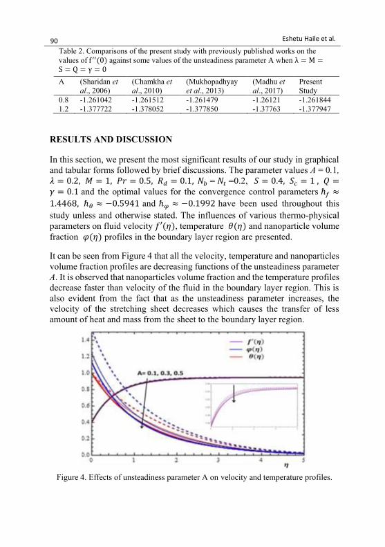
It can be seen from Figure 4 that all the velocity, temperature and nanoparticles

volume fraction profiles are decreasing functions of the unsteadiness parameter

A. It is observed that nanoparticles volume fraction and the temperature profiles

decrease faster than velocity of the fluid in the boundary layer region. This is

also evident from the fact that as the unsteadiness parameter increases, the

velocity of the stretching sheet decreases which causes the transfer of less

amount of heat and mass from the sheet to the boundary layer region.

Figure 4. Effects of unsteadiness parameter A on velocity and temperature profiles.

91 Ethiop. J. Sci. & Technol. 13(2): 81-97 , June 2020

The effects of the Maxwell viscoelastic parameter 𝜆 has been studied and

presented in Figure 5. It can be observed that the temperature and nanoparticles

volume fraction profiles can be enhanced by increasing the parameter 𝜆. On the

other hand, the velocity falls rapidly with increasing values of 𝜆. Physically,

this corresponds to the fact that as 𝜆 increases, the fluid is getting thicker.

Figure 5. Impacts of λ on velocity, temperature and concentration profiles.

Figure 6. Effects of M on velocity, temperature and concentration profiles.

Impacts of the external magnetic field in the flow field has been studied and

presented in Figure 6. The results in the figure display that the increase in

external magnetic field slows down the fluid velocity but it enhances the

92 Eshetu Haile et al.

nanoparticles volume fraction and temperature profiles. This is true as the

increase in magnetic field produces a resistive force, called the Lorentz force,

which retards the motion of the fluid. On the other hand, this resistive force

causes the increase in the temperature and nanoparticles volume fraction in the

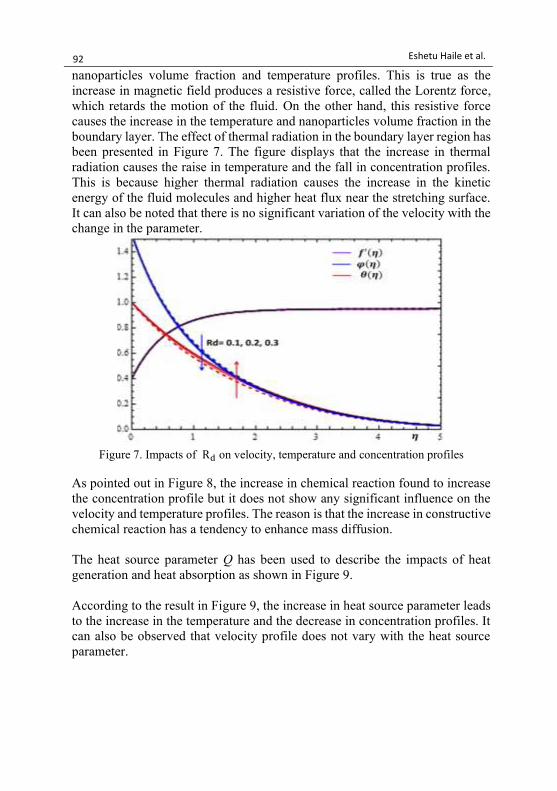
boundary layer. The effect of thermal radiation in the boundary layer region has

been presented in Figure 7. The figure displays that the increase in thermal

radiation causes the raise in temperature and the fall in concentration profiles.

This is because higher thermal radiation causes the increase in the kinetic

energy of the fluid molecules and higher heat flux near the stretching surface.

It can also be noted that there is no significant variation of the velocity with the

change in the parameter.

Figure 7. Impacts of Rd on velocity, temperature and concentration profiles

As pointed out in Figure 8, the increase in chemical reaction found to increase

the concentration profile but it does not show any significant influence on the

velocity and temperature profiles. The reason is that the increase in constructive

chemical reaction has a tendency to enhance mass diffusion.

The heat source parameter Q has been used to describe the impacts of heat

generation and heat absorption as shown in Figure 9.

According to the result in Figure 9, the increase in heat source parameter leads

to the increase in the temperature and the decrease in concentration profiles. It

can also be observed that velocity profile does not vary with the heat source

parameter.

93 Ethiop. J. Sci. & Technol. 13(2): 81-97 , June 2020

Figure 8. Effects ofγon velocity, temperature and concentration profiles.

Figure 9. Effects of Q on velocity, temperature and concentration profiles.

The permeability effect of the stretching sheet has been examined and

illustrated in Figure 10. It can be seen from Figure 10 that both the temperature

and nanoparticles volume fraction profiles are decreasing while the velocity

profile is increasing with the increase in the permeability parameter. The

impacts of some pertinent parameters on local skin friction coefficient (𝐶𝑓),

Nusselt number ( 𝑁𝑢𝑥 ) and Sherwood number ( 𝑆ℎ𝑥 ) were examined and

expressed in terms of the coefficients 𝑓′′(0), −𝜃′(0)and −𝜑′(0), respectively.

94 Eshetu Haile et al.

The variations of skin friction coefficient for different values of some

parameters are plotted in Figures (11-12).

Figure 10. Effects of S on velocity, temperature and concentration profiles.

Figure 11. Variation of skin friction coefficient for different values of the unsteadiness

parameter A along with the heat source parameter Q.

The results in Figure 11-12 indicate that the coefficient of skin friction is

observed to decline as the values of the unsteadiness parameter 𝐴increase along

with the increase in the heat source parameter 𝑄 or the chemical reaction

parameter 𝛾.

Both heat source/sink and chemical reaction parameters have no effect on skin

friction coefficient. Further results on the variations of skin friction coefficient,

95 Ethiop. J. Sci. & Technol. 13(2): 81-97 , June 2020

Nusselt number and Sherwood number with respect to some pertinent

parameters is presented in Table 3.

Figure 12. Variation of skin friction coefficient for different values of the unsteadiness

parameter A along with the chemical reaction parameter γ.

Table 3. Coefficients of Skin-friction, Nusselt number and Sherwood number.

A 𝜆 M 𝑅𝑑 S 𝑆𝑐 Q 𝛾 −𝑓 ′′(0) −𝜃′(0) −𝜑'(0)

0.1 1.58556 0.569631 1.43037

0.2 1.60972 0.637310 1.36269

0.3 0.1 1.63367 0.698930 1.30107

0.2 1.62921 0.564361 1.43564

0.3 1.0 1.71973 0.690822 1.30918

2.0 2.01674 0.669738 1.33026

3.0 0.1 2.27216 0.654251 1.34575

0.2 2.27216 0.617937 1.38206

0.3 0.2 2.27216 0.587700 1.41230

0.3 2.27216 0.587700 1.41230

0.4 1.0 2.38107 0.601453 1.39855

2.0 2.50563 0.620985 1.37901

3.0 0.1 2.50563 0.624377 1.37562

0.2 2.50563 0.591982 1.40802

0.3 0.1 1.81708 0.597492 1.40251

0.2 1.81708 0.597492 1.40251

0.3 1.81708 0.597492 1.40251

One can see from the table that the values of skin friction can be increased by

increasing the unsteadiness parameter A or the magnetic parameter M. The local

Nusselt number can be maximized by increasing the unsteadiness parameter A

or Schmidt number Sc. It can also be enhanced by reducing the magnetic

parameter M or the radiation parameter Rd. Also, the local Sherwood number

96 Eshetu Haile et al.

can be increased by increasing the magnetic parameter M or the radiation

parameter Rd. It can also be increased by reducing the unsteadiness parameter

A or Schmidt number Sc.

CONCLUSION

In this study, efforts were made to improve existing models by considering

additional parameters such as the effects of heat source and chemical reaction

in the flow models. On the other hand, a powerful method, namely the

homotopy analysis method was used and the results agreed with previous

reports. In conclusion, the impacts of pertinent parameters on velocity,

temperature and nanoparticles volume fraction profiles are summarized as

follows:

•The flow velocity can be accelerated by reducing the values of the

unsteadiness, Maxwell viscoelastic, magnetic or permeability parameters;

•The temperature profile can be maximized in the boundary region by

increasing the values of Maxwell, magnetic, permeability or heat source

parameters. This profile can also be enhanced by reducing the effects of

unsteadiness or radiation parameters;

•The concentration of nanoparticles can be raised by increasing the Maxwell,

magnetic, permeability or chemical reaction parameters. The concentration

profile can also be raised by minimizing the unsteadiness, radiation or heat

source parameters. Moreover, the results obtained in the present study were also

found to be in a nice agreement with previous works under some restricted

assumptions.

REFERENCES

Awais, M., Hayat, T., Irum, S and Alsaedi, A. (2015). Heat generation/absorption effects in

a boundary layer stretched flow of Maxwell nanofluid: analytic and numeric solutions.

PLoS One 10(6): DOI: 10.1371/journal.pone.0129814.

Chamkha, J., Aly, M and Mansour, A. (2010). Similarity solution for unsteady heat and mass

transfer from a stretching surface embedded in a porous medium with suction/injection

and chemical reaction effects. Chemical Engineering Communications 197(6): 846-858.

https://doi.org/10.1080/00986440903359087.

Choi, U.S and Eastman, J.A. (1995). Enhancing thermal conductivity of fluids with

nanoparticles. Proceedings of the ASME 66:99–105.

Elbashbeshy, E., Abdelgaber, K and Asker, H. (2018). Heat and mass transfer of a Maxwell

nanofluid over a stretching surface with variable thickness embedded in porous medium.

International Journal of Mathematics and Computational Science 4(3): 86-98.

http://www.aiscience.org/journal/ijmcs

Ijaz, M and Ayub, M. (2019). Nonlinear convective stratified flow of Maxwell nanofluid with

activation energy. Heliyon 5(1): 1-31. DOI: 10.1016/j.heliyon.2019. e01121

97 Ethiop. J. Sci. & Technol. 13(2): 81-97 , June 2020

Liao, J. (2003). Beyond Perturbation: Introduction to Homotopy Analysis Method. Chapman

and Hall/CRC, USA.

Mabood, F., Imtiaz, M., Alsaedi, A and Hayat T. (2016). Unsteady convective boundary layer

flow of Maxwell fluid with nonlinear thermal radiation: A numerical study. International

Journal of Nonlinear Sciences and Numerical Simulation 17(5): 221–229. DOI:

https://doi.org/10.1515/ijnsns-2015-0153. Madhu, M., Kishan, N and Chamkha, J. (2017). Unsteady flow of a Maxwell nanofluid over

a stretching surface in the presence of MHD and thermal radiation effects. Propulsion

and Power Research 6(1):31–40. http://dx.doi.org/10.1016/j.jppr. 2017. 01.002.

Mukhopadhyay, S., Ranjan, P and Layek, G.C. (2013). Heat transfer characteristics for the

Maxwell fluid flow past an unsteady stretching permeable surface embedded in a porous

medium with thermal radiation. Journal of Applied Mechanics and Technical Physics

54(3): 385–396. DOI: 10.1134/S0021894413030061.

Mukhopadhyay, S and Bhattacharyya K. (2012). Unsteady flow of a Maxwell fluid over a

stretching surface in presence of chemical reaction. Journal of the Egyptian Mathematical

Society 20, 229–234. DOI: 10.1515/ijnsns-2015-0153.

Nadeem, S., UlHaq, R and Khan, H. (2013). Numerical study of MHD boundary layer flow

of a Maxwell fluid past a stretching sheet in the presence of nanoparticles. Journal of the

Taiwan Institute of Chemical Engineers 45:121-126. http://dx.doi.org/10.1016/j.

jtice.2013.04.006.

Ramesh, G.K and Gireesha, B.J. (2014). Influence of heat source/sink on a Maxwell fluid

over a stretching surface with convective boundary condition in the presence of

nanoparticles. Ain Shams Engineering Journal 5: 991–998. http://dx.doi.org/10.1016/

j.asej.2014.04.003.

Sharidan, S., Mahmood, T and Pop, I. (2006). Similarity solutions for the unsteady boundary

layer flow and heat transfer due to a stretching sheet. International Journal of Applied

Mechanics and Engineering 11(3): 647-654.

Sravanthi, C.S and Gorla, R.S. (2018). Effects of heat source/sink and chemical reaction on

MHD Maxwell nanofluid flow over a convectively heated exponentially stretching sheet

using homotopy analysis method. International Journal of Applied Mechanics and

Engineering 23(1):137-159. DOI: 10.1515/ijame-2018-0009.

Zhao, Y and Liao, S.J. (2013). Advances in the homotopy analysis method. World Scientific

Publishing Co. Pte. Ltd., Singapore.