This report represents the work of WPI undergraduate students submitted to the faculty as evidence of completion of a degree requirement. WPI routinely publishes these reports on its website without editorial or peer review. For more information about the projects program at WPI, please

see http://www.wpi.edu/academics/ugradstudies/project-learning.html

HEAT TRANSFER

DEMONSTRATION CART

A Major Qualifying Project

Submitted to the Faculty

of the

WORCESTER POLYTECHNIC INSTITUTE

in partial fulfilment of the requirements for the

Degree of Bachelor of Science

In Mechanical Engineering

Submitted By:

Kyle LeBorgne

Foster Lee

João Maurício Vasconcelos

Robert Wood

Date: April 21, 2016

Keywords

1. Heat Transfer

2. Flow Design

3. Instrumentation

Approved:

Prof. Selçuk Güçeri, PhD, Project Advisor

i

Abstract

Visual aids provide an opportunity for greater conceptual understanding in many

engineering topics. In heat transfer education, such visualization tools are rare, if in practice at

all. The objective of this project is to design and construct a portable device capable of both

demonstrating heat transfer forced and natural convection in real-time, and measuring the

convective heat transfer coefficient ‘h’. Analysis of the design and functional requirements

resulted in the development of a subsonic, insulated wind tunnel. The test chamber of the tunnel

is outfitted with custom manufactured geometry and instruments including thermocouples and

hot wire anemometry for data acquisition. Control of heat flux, air velocity, and test geometry

enables the tunnel to simulate common sample problems found in introductory heat transfer

textbooks. The successful operation of the experiment indicates the device is applicable to a

broad range of configurations, including those that parallel introductory heat transfer problems.

ii

Executive Summary

The convective heat transfer coefficient ‘h’, describes the rate at which heat moves

between a solid geometry and the surrounding fluid. It is not a physical property of a material

such as specific heat or thermal conductivity, nor is it a constant property of fluid dynamics. The

coefficient is dependent on the type of media, gas or liquid, the flow properties such as velocity

and viscosity, and other flow and temperature dependent properties. This concept, with its

infinite variations, can be difficult to visualize and comprehend.

The objective of this project is to design and construct a portable device capable of both

demonstrating heat transfer under forced and natural convection, and measuring the convective

heat transfer coefficient ‘h’. A visual aid of this nature provides an opportunity for greater

conceptual understanding of Isaac Newton’s law of cooling. The control of heat flux, air

velocity, and geometry will allow students to experiment with how changing these variables

affect the transfer coefficient. This device will be applicable to a broad range of configurations,

including those that parallel sample problems found in introductory heat transfer textbooks.

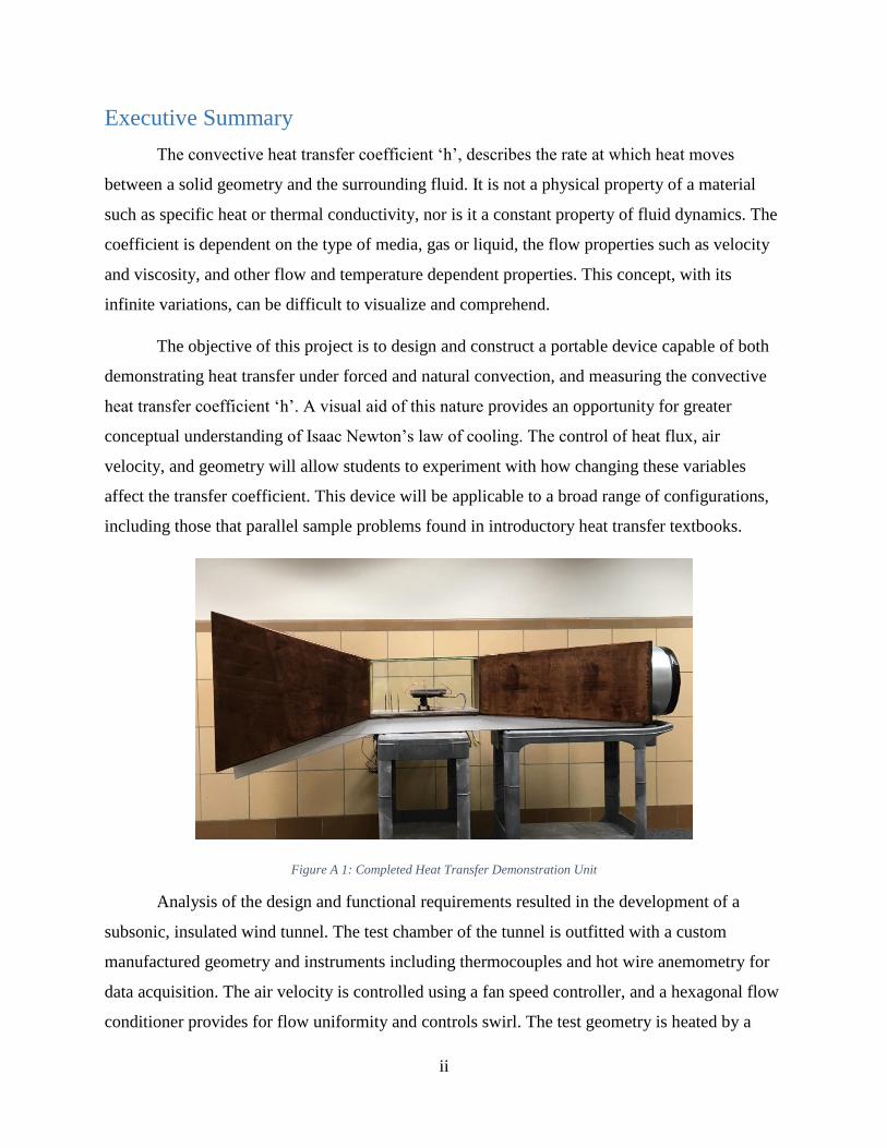
Figure A 1: Completed Heat Transfer Demonstration Unit

Analysis of the design and functional requirements resulted in the development of a

subsonic, insulated wind tunnel. The test chamber of the tunnel is outfitted with a custom

manufactured geometry and instruments including thermocouples and hot wire anemometry for

data acquisition. The air velocity is controlled using a fan speed controller, and a hexagonal flow

conditioner provides for flow uniformity and controls swirl. The test geometry is heated by a

iii

3000 Watt variable autotransformer capable of warming the plate in excess of 400 degrees

Celsius. The device is easily transportable, shown in Figure A1, functioning as a conceptual aid

that can be brought to classrooms to enhance heat transfer education and also as a tool that will

provide opportunities for future analysis.

From the experiments conducted during this project and the results our team collected,

the relationship between the convective heat transfer coefficient and geometric orientation was

interpreted, and conclusions were made about the behavior of ‘h’ as the controlled variables were

manipulated. The team found that higher air velocities corresponded to higher rates of heat

transfer between the two mediums, and subsequently, plate surface temperature decreased. The

analysis of collected data determined that steeper slopes in the test geometry corresponded to

higher rates of heat transfer and thusly higher values of ‘h’, as shown in Figure A2.

Figure A 2: Convective Heat Transfer Coefficient Results

We successfully completed the purpose of this project, demonstrating how to measure the

convective heat transfer coefficient for given configurations within a university lecture hall.

iv

Acknowledgements

We would like to thank the following individuals and organizations for their support and

contributions to the success of the project:

Professor Selçuk Güçeri, PhD, for his continued guidance, enthusiasm, and support as our

project advisor.

Peter Hefti, Engineering Experimentation Lab Manager, for his support and supplying us

with the necessary equipment to collect experimental data.

Professor Jamal Yagoobi, PhD, and Mechanical Engineering Department Head, for

providing the necessary equipment and financial support.

Professor Alexander Emanuel, PhD, for his support with electrical component selection

and instrumentation recommendations.

Christopher Scarpino, Adjunct Instructor, for assisting with LabVIEW programming.

Patricia Howe, Operations Manager, for providing our team with project working space.

Barbara Furhman, Administrative Assistant VI, for purchasing all of our supplies and

processing reimbursement payments.

Aspen Aerogels for donating Pyrogel insulation for use on our project.

Worcester Polytechnic Institute for making our experience on this project possible.

1

Table of Contents

Abstract ............................................................................................................................................ i

Executive Summary ........................................................................................................................ ii

Acknowledgements ........................................................................................................................ iv

Table of Figures .............................................................................................................................. 3

Table of Tables ............................................................................................................................... 4

Chapter 1: Introduction ................................................................................................................... 5

Chapter 2: Background ................................................................................................................... 7

2.1 Methods of Heat Transfer ..................................................................................................... 7

2.1.1 History of the Convective Heat Transfer Coefficient .................................................... 7

2.1.2 The Convective Heat Transfer Coefficient .................................................................... 8

2.1.3 Flow, Boundary Layers, & Convective Heat Transfer .................................................. 8

2.1.4 Textbook Approach to Experimentally Determine Heat Transfer Coefficients .......... 10

2.2 Previous Heat Transfer Coefficient Experiments ............................................................... 12

2.2.1 Comparison of two methods for evaluation fluid to surface heat transfer coefficients 12

2.2.2 High Pressure Die Casting Experiment ....................................................................... 12

2.3 Applications of the Convective Heat Transfer Coefficient ................................................. 13

2.3.1 Aerospace Industry ...................................................................................................... 13

2.3.2 High Pressure Die Casting ........................................................................................... 14

2.3.3 Heating, Ventilation, and Air Conditioning ................................................................. 15

2.3.4 Food Industry ............................................................................................................... 15

2.4 Inspiration for this MQP ..................................................................................................... 16

2.5 Active Learning in Engineering Education ......................................................................... 16

2.5.1 History of Active Learning .......................................................................................... 17

2.5.2 Heat Transfer Courses.................................................................................................. 18

2.5.3 Heat Transfer Experiments .......................................................................................... 18

Chapter 3: Methodology ............................................................................................................... 21

3.1 Subsonic Wind Tunnel Design ........................................................................................... 21

3.1.1 Design Process ............................................................................................................. 21

3.1.2 Introduction to Subsonic Wind Tunnels ...................................................................... 24

3.1.3 Research ....................................................................................................................... 25

2

3.1.4 Computational Testing ................................................................................................. 29

3.1.5 Design Limitations ....................................................................................................... 33

3.2 Measurement and Instrumentation ...................................................................................... 34

3.2.1 Thermocouples ............................................................................................................. 35

3.2.2 Hot-Wire Anemometer ................................................................................................ 37

3.2.3 LabVIEW and DAQ Box ............................................................................................. 37

3.3 Experimentation .................................................................................................................. 40

3.3.1 Circuit Configuration ................................................................................................... 40

3.3.2 Experimental Procedures ............................................................................................. 40

Chapter 4: Results and Analysis ................................................................................................... 47

4.1 MATLAB Prediction and Experimental Result for ΔT vs. Power ..................................... 47

4.2 MATLAB Prediction vs. Experimental Data ...................................................................... 49

4.3 Plate Orientation Angle Experiment ................................................................................... 50

4.4 Power vs. Heat Transfer Coefficient Experiment ............................................................... 51

4.5 General Heat Transfer Coefficient Experiment Data.......................................................... 52

4.6 Possible Sources of Experimental Error ............................................................................. 53

Chapter 5: Conclusion and Recommendations ............................................................................. 54

References ..................................................................................................................................... 55

Appendix A: Construction ............................................................................................................ 57

Appendix B: Instrumentation and Unit Setup ............................................................................... 62

Appendix C: LabVIEW Program .................................................................................................. 68

Appendix D: Data Files ................................................................................................................ 71

Appendix E: Additional MATLAB Generated Result’s Graphs .................................................. 73

Appendix F: ANSYS Generated Fluent Report ............................................................................ 76

Appendix G: Textbook Sample Problem ...................................................................................... 87

3

Table of Figures

Figure 1: Flat Plate in Parallel Flow (Bergman, Levine, Incropera, Dewitt, 2011) ........................ 9

Figure 2: Example Honeycomb Laminar Flow Straightener Courtesy of Saxonpc.com ............. 10

Figure 3: Boeing's Autoclave. Source: aviation-images.com ....................................................... 14

Figure 4: Example Applet Activity from Tan & Fok, 2009 ......................................................... 19

Figure 5: Example results from figure 4 above by Tan & Fok, 2009 ........................................... 19

Figure 6: Early Design Iteration ................................................................................................... 23

Figure 7: Nozzle CAD Image ....................................................................................................... 27

Figure 8: Diffuser CAD Image ..................................................................................................... 27

Figure 9: Final CAD Assembly .................................................................................................... 28

Figure 10: Three Dimensional Vorticity Simulation .................................................................... 29

Figure 11: Velocity vs Distance .................................................................................................... 30

Figure 12: Pressure vs Distance .................................................................................................... 31

Figure 13: Velocity Profile ........................................................................................................... 31

Figure 14: Pressure Gradient ........................................................................................................ 32

Figure 15: Turbulence Check........................................................................................................ 33

Figure 16: Thermocouples positioned according to letter type .................................................... 36

Figure 17: Frame of one stacked sequence gathering data for one thermocouple ........................ 38

Figure 18: Calculation of the heat transfer coefficient in the LabVIEW program ....................... 39

Figure 19: Write-to-file and tab labels on block diagram ............................................................. 39

Figure 20: Variac Circuit Configuration ....................................................................................... 40

Figure 21: 15 Degree Orientation Angle ...................................................................................... 44

Figure 22: 30 Degree Orientation Angle ...................................................................................... 45

Figure 23: Predicted Q as a Function of ΔT and Air Velocity ..................................................... 48

Figure 24: Experiment Results: Q as a Function of ΔT and Air Velocity .................................... 48

Figure 25: At left, predicted ΔT vs. ‘h’. At right, Experimental data ΔT vs. ‘h’. ........................ 49

Figure 26: Experimental data ΔT vs. ‘h’ superimposed onto predicted ΔT vs. ‘h’ ...................... 49

Figure 27: 'h' as a Function of Air Velocity .................................................................................. 50

Figure 28: 'h' as a Function of Air Velocity and Power ................................................................ 51

4

Table of Tables

Table 1: Thermocouple Types ...................................................................................................... 36

Table 2: General 'h' Coefficients for Air Velocity and Power ...................................................... 52

5

Chapter 1: Introduction

As the demand for highly skilled workers and engineer’s increases, so does the need to

educate up and coming generations in the most effective way possible. In an age where there is

so much to learn in only four years of high level schooling, finding the best ways to present

information to students is key. Getting hands on experience and witnessing the magic of modern

science not only reinforces understanding but excites and inspires students to discover.

The objective of this project is to design and construct a portable device capable of both

demonstrating heat transfer under forced and natural convection, and measuring the convective

heat transfer coefficient ‘h’. A visual aid of this nature provides an opportunity for greater

conceptual understanding of Isaac Newton’s law of cooling. The control of heat flux, air

velocity, and geometry will allow students to experiment with how changing these variables

affect the transfer coefficient. This device will be applicable to a broad range of configurations,

including those that parallel sample problems found in introductory heat transfer textbooks. The

device is easily transportable, functioning as a conceptual aid that can be brought to classrooms

to enhance heat transfer education and also as a tool that will provide opportunities for future

analysis.

The heat transfer coefficient is an essential building block of thermodynamics. Without

the study of its properties we could not have modern tools and technologies. Construction of air

plane wings, easy access to food in the marketplace, and the ability to heat and cool our

environment all require mathematical computation to estimate this ‘h’ value.

The convective heat transfer coefficient, ‘h’, changes drastically under different

conditions. It is not a physical property of a material such as specific heat or thermal

conductivity, nor is it a constant property of fluid dynamics. The coefficient is dependent on the

type of media, gas or liquid, the flow properties such as velocity and viscosity, and other flow

and temperature dependent properties. In simple terms, it describes the rate at which heat moves

between a solid geometry and the surrounding fluid. This concept, with its infinite variations, can

be difficult to visualize and comprehend. This is the primary motivation behind our project and

why visual demonstration was taken into account in the design process. Our team will also

include recommendations for future development and research opportunities.

6

This paper will introduce the fundamental elements of heat transfer and the equations that

govern the convective heat transfer coefficient. It will discuss the experiments our team

conducted and include an analysis of the relationship between the controlled variables and the

convection coefficient. We will outline our procedure for designing our project, how we

constructed it, and our approach to experimentally investigating the properties of ‘h’. Data from

the experiments our team conducted will be discussed and analyzed, and conclusions will be

drawn from our results.

7

Chapter 2: Background

To develop an enhanced understanding of heat transfer experiments, research of several

experimental methods provided a foundation upon which an experimental design could be

prepared. The following research and background information will provide insight into

fundamental concepts, methods, and previous experiments. To begin, research on general heat

transfer and the convective heat transfer coefficient including its history, proved meaningful

when understanding design constraints. Additional detailed research into boundary conditions

affects, previous experimental efforts, and convective applications provides validity to the

research project. Lastly, investigation into active learning in engineering education pertaining to

how this particular project will create opportunities in WPI’s classrooms for generations.

2.1 Methods of Heat Transfer

Heat transfer is the process of thermal energy transfer due to a temperature difference in a

medium or mediums. “Whenever a temperature difference exists in a medium or between media,

heat transfer must occur” (Bergman, Lavine, Incropera, Dewitt, 2011). There are three

conventional methods of heat transfer: conduction, convection, and thermal radiation.

Conduction occurs where heat is transferred across a medium. Convection refers to heat transfer

between a solid surface and a moving fluid. Heat transferred between mediums by way of

electromagnetic waves is called thermal radiation. Any surface at a fixed temperature emits

energy in the form of electromagnetic waves. (Bergman, Lavine, Incropera, Dewitt, 2011)

2.1.1 History of the Convective Heat Transfer Coefficient

“Isaac Newton is widely credited with the following statement of the convective heat

transfer coefficient:

𝑞 = ℎ𝐴(𝑇𝑠𝑢𝑟 − 𝑇𝑠𝑢𝑟𝑟)

Where q is the rate of heat transfer, h the heat transfer coefficient, A the surface area, 𝑇𝑠𝑢𝑟 the

surface temperature, and 𝑇𝑠𝑢𝑟𝑟 the temperature of the surroundings (Bergles 1988)”. Isaac

Newton was a pioneer in the field of heat transfer, publishing papers in the early eighteenth

century. Newton published a paper in 1701 that included the formula above. The historical

accuracy of the statement above is under criticism from many scientists because Newton’s paper

does not specifically identify a proportional constant between heat flux and temperature

8

difference. The equation is often referenced as “Newton’s Law of Cooling”, leading to the

conclusion Newton was instrumental in the development of convective heat transfer coefficient.1

2.1.2 The Convective Heat Transfer Coefficient

The heat transfer coefficient, h, is an essential quantity used in the calculation of heat

transfer, generally used when there is a phase change between a fluid and a solid, or convection.

The coefficient is not a physical property such as specific heat or thermal conductivity, but rather

a descriptive quantity based on fluids interacting with geometries. As a fluid moves across a

geometry, an extremely thin layer of the fluid “sticks” to the surface, resulting in heat

transferring between the two mediums. “The convective heat transfer coefficient depends on

conditions in the boundary layer, which are influenced by surface geometry, the nature of fluid

motion, and an assortment of fluid thermodynamic and transport properties. Any study of

convection ultimately reduces to a study of the means by which h may be determined”

(Bergman, Lavine, Incropera, Dewitt, 2011). To determine h for critical components the

calculation needs to be completed experimentally.

The convective heat transfer coefficient can be isolated, represented by the equation

below.

𝐶𝑜𝑛𝑣𝑒𝑐𝑡𝑖𝑣𝑒 𝐻𝑒𝑎𝑡 𝑇𝑟𝑎𝑛𝑠𝑓𝑒𝑟 𝐶𝑜𝑒𝑓𝑓𝑖𝑐𝑖𝑒𝑛𝑡 = ℎ =𝑞

𝐴(𝑇𝑠𝑢𝑟 − 𝑇𝑠𝑢𝑟𝑟)

The variable “q” is the convective heat flux, representing the proportional difference between the

temperatures of the surface, 𝑇𝑠𝑢𝑟, and the surrounding area, 𝑇𝑠𝑢𝑟𝑟. The SI standard units for h, is

watts per square meter kelvin W/(m2°K).

2.1.3 Flow, Boundary Layers, & Convective Heat Transfer

The two methods of convective heat transfer include natural and forced convection. In

natural convection the fluid surrounding the hot surface is not moving by an external force,

rather the buoyancy force created by the temperature gradient causes the motion. In forced

convection, the fluid is moving relative to the hot surface by an external force, for example a

pump or fan. (Bergman, Lavine, Incropera, Dewitt, 2011) Flow refers to the motion of a fluid

1 Enhancement of Convective Heat Transfer: Newton’s Legacy Pursued. Arthur E. Bergles.

9

over a surface with relatively velocity. Flow can be either laminar, layered flow without mixing

between the layers, or turbulent, flow chaotic in nature with rapid property changes. The

experiments conducted by our team will include flow across a heated flat plate, known as

external flow. In external flow environments, there are no constraints imposed by adjacent

surfaces, allowing boundary conditions to develop freely. (Bergman, Lavine, Incropera, Dewitt,

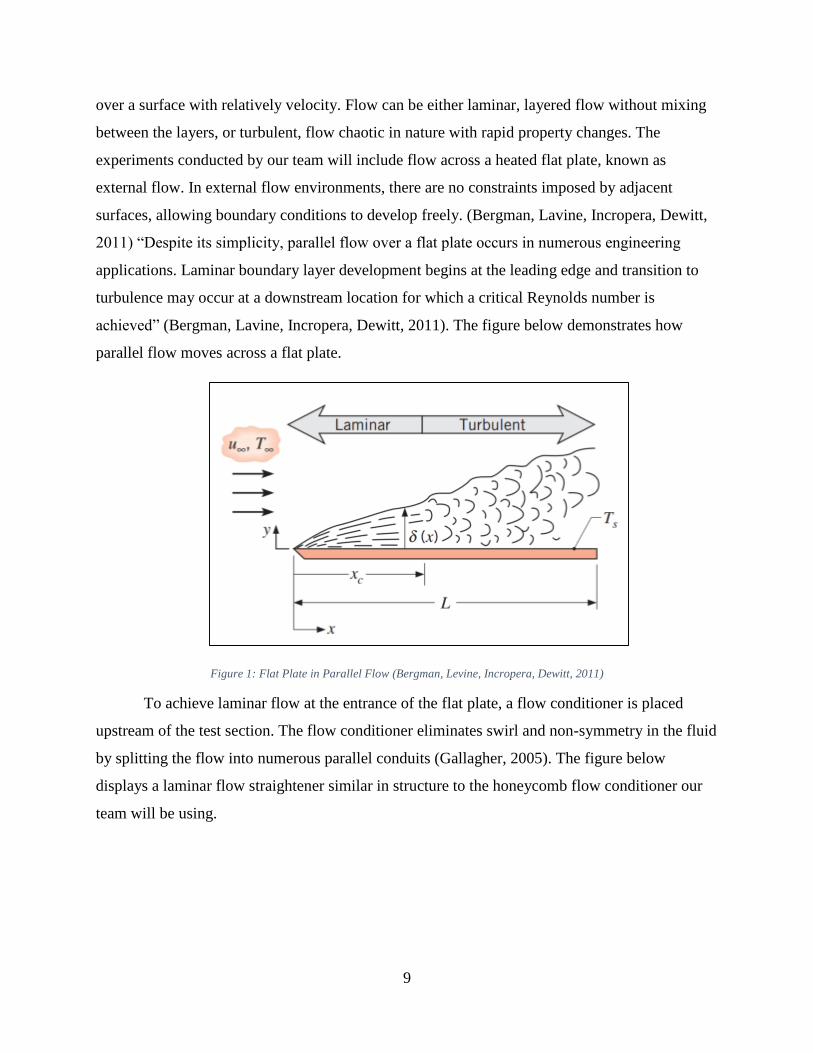
2011) “Despite its simplicity, parallel flow over a flat plate occurs in numerous engineering

applications. Laminar boundary layer development begins at the leading edge and transition to

turbulence may occur at a downstream location for which a critical Reynolds number is

achieved” (Bergman, Lavine, Incropera, Dewitt, 2011). The figure below demonstrates how

parallel flow moves across a flat plate.

Figure 1: Flat Plate in Parallel Flow (Bergman, Levine, Incropera, Dewitt, 2011)

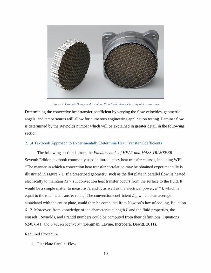
To achieve laminar flow at the entrance of the flat plate, a flow conditioner is placed

upstream of the test section. The flow conditioner eliminates swirl and non-symmetry in the fluid

by splitting the flow into numerous parallel conduits (Gallagher, 2005). The figure below

displays a laminar flow straightener similar in structure to the honeycomb flow conditioner our

team will be using.

10

Figure 2: Example Honeycomb Laminar Flow Straightener Courtesy of Saxonpc.com

Determining the convective heat transfer coefficient by varying the flow velocities, geometric

angels, and temperatures will allow for numerous engineering application testing. Laminar flow

is determined by the Reynolds number which will be explained in greater detail in the following

section.

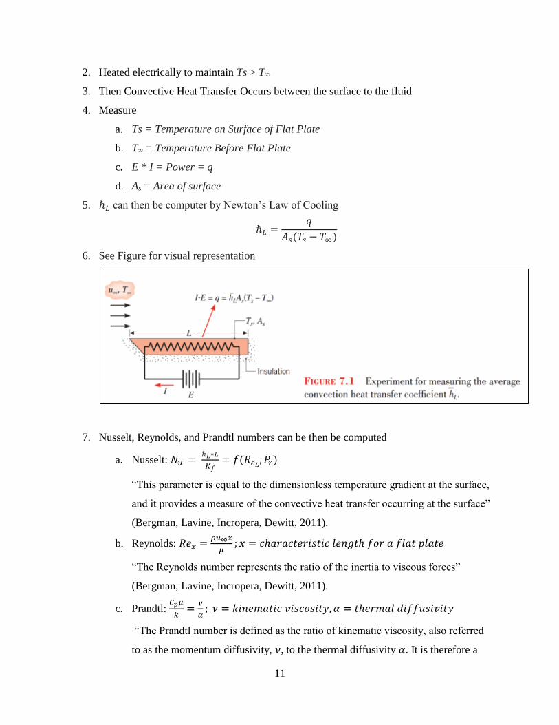
2.1.4 Textbook Approach to Experimentally Determine Heat Transfer Coefficients

The following section is from the Fundamentals of HEAT and MASS TRANSFER

Seventh Edition textbook commonly used in introductory heat transfer courses, including WPI.

“The manner in which a convection heat transfer correlation may be obtained experimentally is

illustrated in Figure 7.1. If a prescribed geometry, such as the flat plate in parallel flow, is heated

electrically to maintain Ts > T∞, convection heat transfer occurs from the surface to the fluid. It

would be a simple matter to measure Ts and T, as well as the electrical power, E * I, which is

equal to the total heat transfer rate q. The convection coefficient ℏ𝐿, which is an average

associated with the entire plate, could then be computed from Newton’s law of cooling, Equation

6.12. Moreover, from knowledge of the characteristic length L and the fluid properties, the

Nusselt, Reynolds, and Prandtl numbers could be computed from their definitions, Equations

6.50, 6.41, and 6.42, respectively” (Bergman, Lavine, Incropera, Dewitt, 2011).

Required Procedure

1. Flat Plate Parallel Flow

11

2. Heated electrically to maintain Ts > T∞

3. Then Convective Heat Transfer Occurs between the surface to the fluid

4. Measure

a. Ts = Temperature on Surface of Flat Plate

b. T∞ = Temperature Before Flat Plate

c. E * I = Power = q

d. As = Area of surface

5. ℏ𝐿 can then be computer by Newton’s Law of Cooling

ℏ𝐿 =𝑞

𝐴𝑠(𝑇𝑠 − 𝑇∞)

6. See Figure for visual representation

7. Nusselt, Reynolds, and Prandtl numbers can be then be computed

a. Nusselt: 𝑁𝑢 = ℏ𝐿∗𝐿

𝐾𝑓= 𝑓(𝑅𝑒𝐿

, 𝑃𝑟)

“This parameter is equal to the dimensionless temperature gradient at the surface,

and it provides a measure of the convective heat transfer occurring at the surface”

(Bergman, Lavine, Incropera, Dewitt, 2011).

b. Reynolds: 𝑅𝑒𝑥 =𝜌𝑢∞𝑥

𝜇; 𝑥 = 𝑐ℎ𝑎𝑟𝑎𝑐𝑡𝑒𝑟𝑖𝑠𝑡𝑖𝑐 𝑙𝑒𝑛𝑔𝑡ℎ 𝑓𝑜𝑟 𝑎 𝑓𝑙𝑎𝑡 𝑝𝑙𝑎𝑡𝑒

“The Reynolds number represents the ratio of the inertia to viscous forces”

(Bergman, Lavine, Incropera, Dewitt, 2011).

c. Prandtl: 𝐶𝑝𝜇

𝑘=

𝜈

𝛼; 𝜈 = 𝑘𝑖𝑛𝑒𝑚𝑎𝑡𝑖𝑐 𝑣𝑖𝑠𝑐𝑜𝑠𝑖𝑡𝑦, 𝛼 = 𝑡ℎ𝑒𝑟𝑚𝑎𝑙 𝑑𝑖𝑓𝑓𝑢𝑠𝑖𝑣𝑖𝑡𝑦

“The Prandtl number is defined as the ratio of kinematic viscosity, also referred

to as the momentum diffusivity, 𝜈, to the thermal diffusivity 𝛼. It is therefore a

12

fluid property. The Prandtl number provides a measure of the relative

effectiveness of momentum and energy transport by diffusion in the velocity and

thermal boundary layers, respectively” (Bergman, Lavine, Incropera, Dewitt,

2011).

2.2 Previous Heat Transfer Coefficient Experiments

Discovered centuries ago, the heat transfer coefficient has been the focus of many

previous research experiments conducted by large universities. Our team researched previous

experimental methods; similar to the process we conducted, along with analytical methods to

demonstrate alternative research techniques.

2.2.1 Comparison of two methods for evaluation fluid to surface heat transfer coefficients

An investigation conducted by the Department of Food Science and Agriculture at

McGill University researched two analytical methods to accurately determine the convective

heat transfer coefficients, while varying heating and cooling environments across three sample

shapes (Awuah, Ramaswamy, Simpson, 1995). “Heat transfer coefficients are commonly

evaluated from time-temperature data obtained from test objects of known shape, size and

thermal properties. Of the two methods commonly used, both based on analytical solution to

transient heat conduction equation, the first (rate method) is based on relating hfs (Convective

heat transfer coefficient (W/m2°C)) to the rate of heating at a given location in the product. The

second (ratio method) is based on relating hfs to the temperature lag between two locations in the

test object. Both methods require accurate thermophysical properties as input parameters”

(Awuah, Ramaswamy, Simpson, 1995). The results illustrate similar hfs values for

experimentally identical conditions, particularly in situations where Biot numbers were low. The

range of calculated values stretched between 15 and 420 W/m2°C depending on the test

conditions (Awuah, Ramaswamy, Simpson, 1995). The report concluded, “Overall, the rate

method gave more consistent and conservative hfs values” (Awuah, Ramaswamy, Simpson,

1995).

2.2.2 High Pressure Die Casting Experiment

Our team’s goal to create an active learning approach to heat transfer courses, lead to

design of a physical heat transfer experiment with a comparable method to the following study

13

funded by the National Science Foundation of China. “In this study, the IHTC (interfacial heat

transfer coefficient) in the HPDC (high pressure die casting) process was determined based on

the temperature measurements inside the die. The IHTC was then used as the boundary condition

for the determination of the thermal field of the casting. Based on the simulated temperatures the

pressure distribution inside the casting was determined. The metal/die interfacial heat transfer

coefficient was successfully determined based on the measured temperature inside the die by

solving the inverse heat transfer problem. The simulated results were found to be in reasonable

agreement with the experimental data” (Guo, Xiong, Liu, Li, Allison, 2009).

2.3 Applications of the Convective Heat Transfer Coefficient

The coefficient is not a term only used by scientist in labs, or taught in engineering

classes, it is relevant in numerous industries. The convective heat transfer coefficient has vital

applications within the aerospace, food, HVAC, and metalworking industries. Any industry

where media is heated or cooled will most likely estimate and use the convective heat transfer

coefficient. The following are four examples of industries requiring frequent heat transfer.

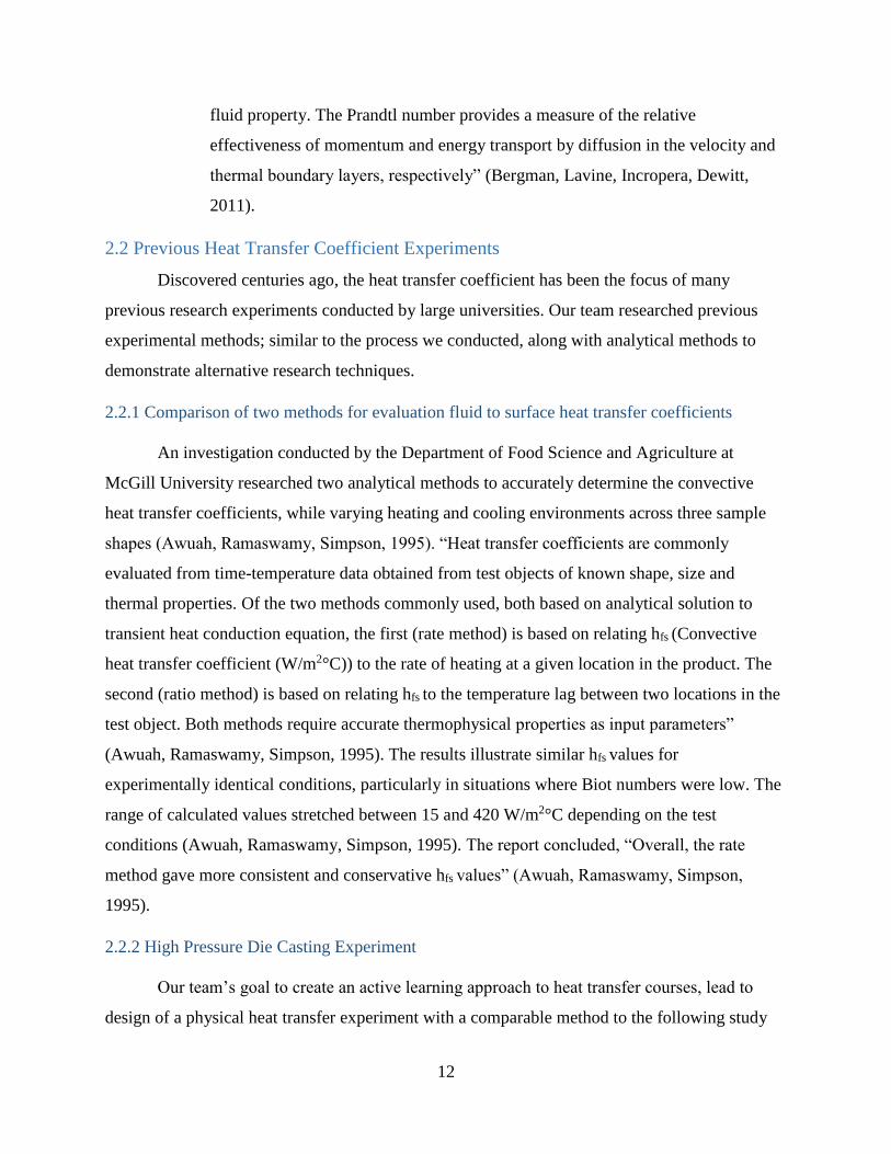
2.3.1 Aerospace Industry

Products of the aerospace industry have tremendous heat transfer requirements, and the

calculations require accurate h values. Boeing, a leading passenger aircraft manufacturer,

recently developed a predominantly carbon composite aircraft, the Boeing 787 Dreamliner. The

carbon composite wings need to bake in an enormous autoclave to cure the epoxy resin and the

carbon fibers. Aircraft manufacturers previously used machining to construct components,

resulting in high waste costs. Current carbon fiber composite construction removes the

machining process, allowing the manufacture to shape the material to exact component

specifications, removing waste from the process. Each wing needs to bake as one unit, and

contains millions of dollars’ worth of carbon fiber composite. The convective heat transfer

coefficient is a crucial value, which needs to be calculated experimentally to determine proper

curing of the composite. The 787’s wing demonstrates the sophisticated and financially

significant implications in correctly determining the convective heat transfer coefficient between

a fluid and surface. The image below demonstrates the enormity of Boeing’s autoclave.

14

Figure 3: Boeing's Autoclave. Source: aviation-images.com

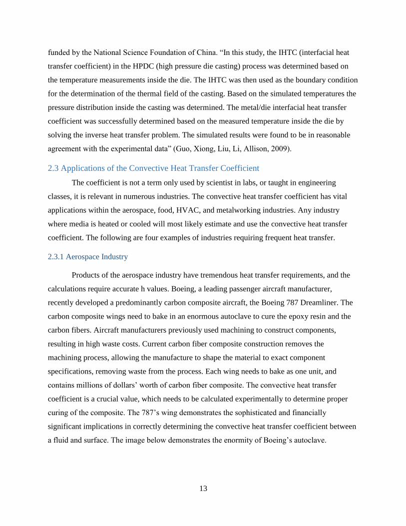
Temperatures can vary greatly between points on a surface undergoing thermal stresses.

When Boeing uses heat to cure its aircraft wings, local minumim and maximum temperature

values form on the surface of the wing. The graphic below demostrates an example temerature

distribution of a model aircraft wing, displaying the differences in maxima and minima in

temperature.

2.3.2 High Pressure Die Casting

High Pressure Die Casting (HPDC) is rapidly becoming the leading method for producing

aluminum and magnesium alloy components in industry. The HPDC method is extremely

efficient and allows for altercation of the alloy’s microstructure to improve component

performance. “During the solidifications process, the microstructure of the casting is highly

15

dependent on the heat transfer process (which is characterized by the interfacial heat transfer

coefficient (IHTC) at the metal/die interface” (Guo, Xiong, Liu, Li, Allison, 2009).

2.3.3 Heating, Ventilation, and Air Conditioning

The overall heat transfer coefficient (U-value) is crucial to determine how heat is

transferred between a building envelope and the outside environment. The U-Value is comprised

of the individual convective heat transfer coefficients of each fluid present in the system,

examples include air inside the building, air outside the building, and air in-between window

glass if more than one plane is present. Additional components include the thermal conductivity

and thickness of the building envelope materials and the contact areas. “The knowledge of the U-

Value is a precondition for the classification of the energy performance of existing buildings”

(Fokaides, Kalogirou, 2011). While the convective heat transfer coefficient is only a portion of

the overall coefficient, it does have significant implications in HVAC and building performance.

2.3.4 Food Industry

“The surface heat transfer coefficient h is a key parameter in the calculation of

heating/chilling time, and hence in the design of facilities for thermal treatments of foods (hydro-

cooling, air-cooling, cooking, etc.)” (Cuesta, Lamua, Alique, 2011). The food industry often uses

large refrigeration and freezing units to chill foods to a lower temperature in preparation for

storage or transportation. The refrigeration units, commonly referred to as chillers, use natural

convection when fans do not assist circulation. Convection is significant when hot surfaces are

exposed to cooler ambient air, commonly found in all facets of the food industry. When material

is placed into the oven, and when material is removed from oven, convection significantly

influences cooking and cooling of the material. “The increased consumer demand for high

quality, nutritious and safe products at affordable prices has resulted in a need to minimize the

severity of heat treatments without compromising safety” (Awuah, Ramaswamy, Simpson,

1995). Common kitchen techniques including baking, cooking, canning, steaming, and curing all

require heat transfer leading to the development of new methods for determining thermal

processes.

16

2.4 Inspiration for this MQP

The heat transfer course required for a Mechanical Engineering major at WPI is lecture

based. The class does not include a lab section where hands-on heat transfer experiments can be

conducted. Our team believes hands-on learning is essential for the modern student to entirely

comprehend subject matter. WPI’s motto is “Lehr und Kunst”, German for theory and practice;

however, a majority of the engineering science classes do not incorporate a practical element to

the course. Upon further investigation and discussion with university officials, limited adequate

lab space on campus is the primary reason for the deficiency in practical hands-on experiments.

The principal motive for this MQP was to create an experimental unit that will allow students

enrolled in WPI’s heat transfer courses to preform experiments within the classroom. The idea of

a demonstration unit was conceived during a discussion with Professor Guceri where he asked

students for feedback on his heat transfer course. Professor Guceri was interested in student

suggestions to improve the course in the future

Our team is creating a device that will bring the laboratory to the classroom and expose

students to theory and practice simultaneously, allowing for comprehensive active learning

content and demonstrations to be incorporated in introductory heat transfer courses.

2.5 Active Learning in Engineering Education

Active learning is a relatively new approach to teaching at the higher educational

institutions. Active learning involves students participating in course by doing more than just

listening; therefore, “They must read, write, discuss, or be engaged in solving problems. Most

important, to be actively involved, student must engage in such higher-order thinking tasks as

analysis, synthesis, and evaluation” (Bonwell, Eison, 1991). Traditional learning environments

involve a formal lecture from a professor; students are engaged in the lecture by listening and

recording notes. “Research has demonstrated, for example, that if a faculty member allows

students to consolidate their notes by pausing three times for two minutes each during alecture,

students will learn significantly more information (Ruhl, Hughes, and Schloss 1987). Two other

simple yet effective ways to involve students during a lecture are to insert brief demonstrations

or short, ungraded writing exercises followed by class discussion” (Bonwell, Eison, 1991).

17

2.5.1 History of Active Learning

Active learning became a widely used and accepted approach to education in 1991 when

Charles C. Bonwell and James A. Eison published Active Learning: Creating Excitement in the

Classroom. The United States Department of Education Office of Educational Research and

Improvement sponsored the research and was featured in the Association for the study of Higher

Education and published by The George Washington University School of Education and Human

Development. Active learning faced many barriers at first, most notably from faculty members

and institutions who had perceptions on what higher education means and the traditions

associated with it. Instructors and professors did not have incentives to change curriculum, as

well as the anxiety and discomfort created by change itself (Bonwell, Eison, 1991). “The reform

of instructional practice in higher education must begin with faculty members’ efforts…Faculty

can successfully over-come each of the major obstacles or barriers to the use of active learning

by gradually incorporating teaching strategies requiring more activity from students and/or

greater risk into their regular style of instruction” (Bonwell, Eison, 1991). Throughout the

following decades after the publication of Bonwell and Eison’s report, active learning slowly

began to enter higher education courses. The advance of technology in classrooms increased the

availability of active learning methods to faculty; therefore, leading to adoption of active

learning at many major institutions including Worcester Polytechnic Institute.

Research studies conducted on active learning show promising evidence to the merit

behind the theory of active learning. University physics courses were among the early adopters

of the active learning approach, with numerous major studies displaying supporting statistical

evidence. A survey of 6,542 students in 62 introductory physics courses, showed the 48 courses

using active learning, or interactive engagement techniques, improved student scores by 25

percent to reach an average gain of 48 percent with a standard deviation of 14 on the Force

Concept Inventory, the standard test of physics conceptual knowledge (Hake, 1998). The 14

courses, which did not participate in active learning techniques, achieved an average gain of 23

percent with a standard deviation of four (Hake, 1998). Additionally, a report published by the

American Association of Physics Teachers explains, “When instructors switched their physics

classes from traditional instruction to active learning, student learning improved 28 percent

points, from around 12% to over 50%, as measured by the Force Concept Inventory, which has

18

become the standard measure of student learning in physics courses” (Hoellwarth, Moelter,

2011).

2.5.2 Heat Transfer Courses

Active learning in undergraduate heat transfer courses has been a topic of discussion for

The American Society of Mechanical Engineers (ASME). At the 2008 ASME Summer Heat

Transfer Conference, there were several presentations on new and innovative approaches to

introductory heat transfer courses. Michael Pate presented one technique, often practiced in

courses at WPI, “The method focuses on minimizing lecture time and maximizing student

engagement. Learning is achieved by forming small groups of two to three students who then

work on in-class graded assignments” (ASME, Pate, 2008). Heat transfer courses at WPI use

group projects and in-class assignments to stimulate learning and generate greater outcomes. Our

project aims to advance active learning objectives with real-time experiments and physically

illustrate the concepts explained in the textbook.

2.5.3 Heat Transfer Experiments

One approach to developing interactive projects for heat transfer and thermal courses is

through computer-based applets. The Nanyang Technological University (NTU) has been

conducting research into active learning methods, with a focus on applets. “…Development of

electronic resources for thermal-fluid courses, with a focus on the development of interactive

learning activities for students to explore and discover heat transfer concepts and mechanisms.

Three basic types of Java applets based on the three main types if interactive knowledge

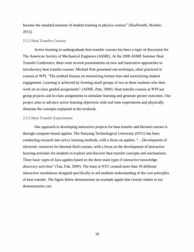
discovery activities” (Tan, Fok, 2009). The team at NTU created more than 30 different

interactive simulations designed specifically to aid students understanding of the core principles

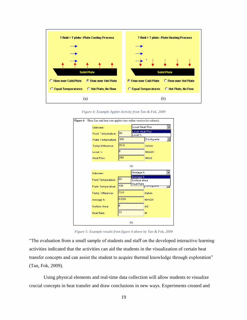
of heat transfer. The figure below demonstrates an example applet that closely relates to our

demonstration cart.

19

Figure 4: Example Applet Activity from Tan & Fok, 2009

Figure 5: Example results from figure 4 above by Tan & Fok, 2009

“The evaluation from a small sample of students and staff on the developed interactive learning

activities indicated that the activities can aid the students in the visualization of certain heat

transfer concepts and can assist the student to acquire thermal knowledge through exploration”

(Tan, Fok, 2009).

Using physical elements and real-time data collection will allow students to visualize

crucial concepts in heat transfer and draw conclusions in new ways. Experiments created and

20

conducted using textbook examples will add a new level of validity to the hypothetical problems

students are asked to solve. Students will gain valuable experimental skills using advanced

instrumentation including thermocouples, hot wire anemometers, inferred thermometers, and

variac transformers. We firmly believe the addition of a heat transfer demonstration cart will

change introductory heat transfer courses at WPI and contribute to the advancement of active

learning methods.

21

Chapter 3: Methodology

3.1 Subsonic Wind Tunnel Design

3.1.1 Design Process

The heat flux caused by forced convection is given by the following equation:

𝑄𝑐𝑜𝑛𝑣 = ℎ𝐴(𝑇𝑠 − 𝑇𝑖𝑛𝑓)

Where 𝑄𝑐𝑜𝑛𝑣 is heat flux, h is the convective heat transfer coefficient, A is surface area,

𝑇𝑠 is surface temperature, and 𝑇𝑖𝑛𝑓 is ambient temperature. With knowledge of this equation, it

can be easily understood that by controlling heat flux via controlling input power to a system,

recording surface area of a test configuration, and measuring both configuration surface

temperature and ambient temperature, an experiment can be carried out for the purpose of

finding the heat transfer coefficient ‘h’ for that specific configuration.

Axiomatic design was utilized for the purpose of defining project requirements.

Axiomatic design is a design methodology requiring matrices to lay out independent functional

requirements of a design, and link them to design parameters and process variables (Suh, 1990).

The link between functional requirements and design parameters is visualized in the equation

below.

[𝐹𝑅1𝐹𝑅2

] = [𝐴] [𝐷𝑃1𝐷𝑃2

]

Where the A matrix is known as the design matrix.

In designing this project, functional requirements, or FRs, and design parameters, or

DPs, were used to eliminate poor designs early in the design process.

The functional requirements for the system are as follows:

FR1: The system must be capable of experimentally measuring the heat transfer

coefficient ‘h’ for configurations that parallel sample heat transfer textbook problems.

FR2: The system must not noticeably affect the ambient conditions of the room in which

it is operated.

22

Where the rooms ambient conditions are comprised of temperature, noise to a reasonable degree,

and air velocity to a reasonable area of influence should air be used as the systems convective

medium. The design parameters were then selected to be the following:

DP1: The system will regulate input power, make use of configuration surface area, and

measure surface and ambient temperatures.

DP2: The system shall be insulated and closed in sections that are likely to affect ambient

conditions.

The first functional requirement, FR1, is broken down to the following elements:

FR11: The system must provide for laminar flow at the leading edge of the test geometry.

FR12: The system must allow for multiple configuration surface temperatures.

FR13: The system must allow for multiple convective medium velocities.

Likewise, the second functional requirement is then broken down.

FR21: The system must not noticeably affect the temperature of the environment in

which it operates.

FR22: The system must not produce an uncomfortable amount of audible noise

Given these expanded functional requirements, design parameters are defined. The first

design parameter, DP1, expands to the following:

DP11: Presence of a flow conditioning system that ensures laminar flow for the full range

of convective medium velocities.

DP12: Installation of a user-controlled heating element tied to the test geometry capable

of generating temperatures from at least room temperature to 200˚C.

DP13: Installation of a user-controlled pump or fan for convective medium velocity

control for a velocity range of at least .5 m/s to 5 m/s.

Similarly, the second design parameter expands to the following:

23

DP21: The system shall be insulated and closed in select areas such that the temperature

immediately surrounding the system does not change by more than 3˚C.

DP22: The system must not produce more than 85dBA of noise, which is the level at

which hearing loss can potentially occur if exposure is prolonged (CDC/NIOSH, 1998).

After establishing expanded functional requirements and design parameters, several

design iterations were drafted and measured based on their compliance with the established

axioms.

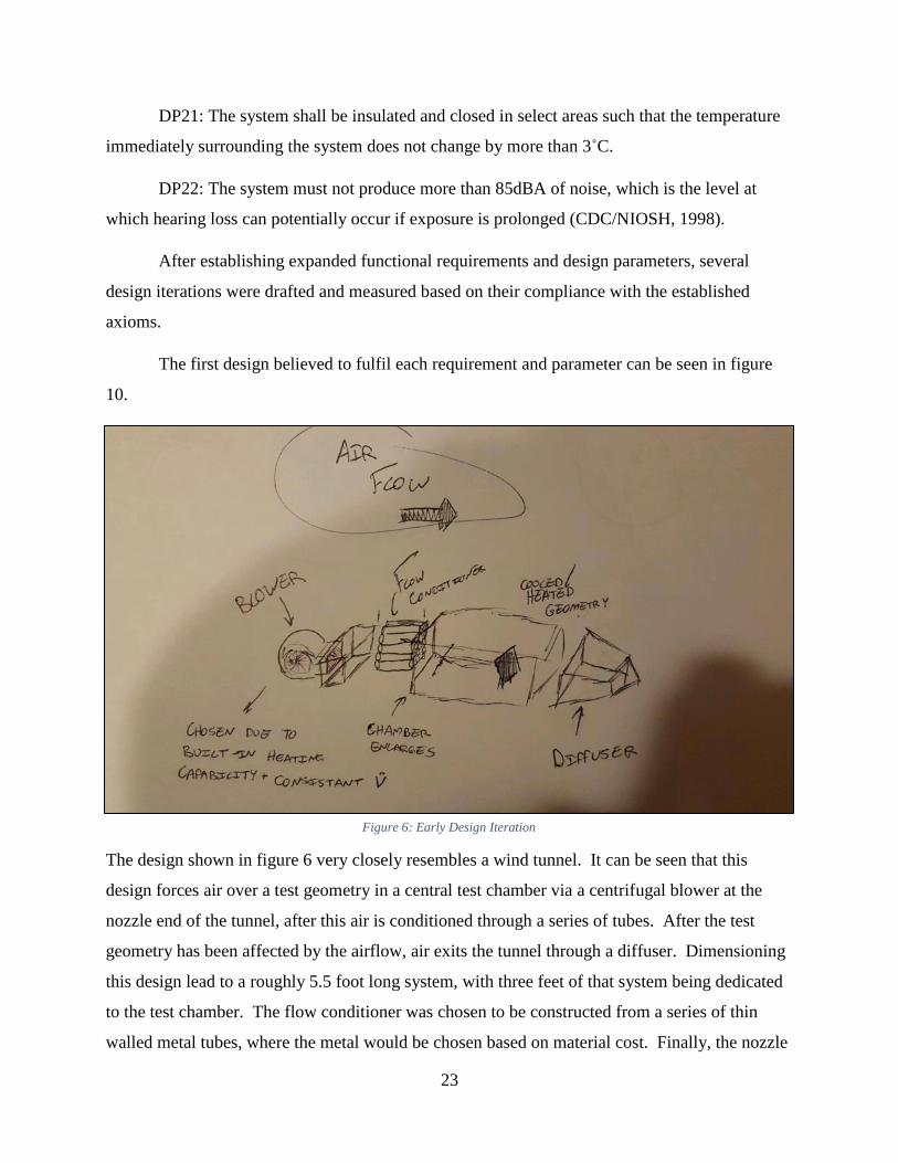
The first design believed to fulfil each requirement and parameter can be seen in figure

10.

The design shown in figure 6 very closely resembles a wind tunnel. It can be seen that this

design forces air over a test geometry in a central test chamber via a centrifugal blower at the

nozzle end of the tunnel, after this air is conditioned through a series of tubes. After the test

geometry has been affected by the airflow, air exits the tunnel through a diffuser. Dimensioning

this design lead to a roughly 5.5 foot long system, with three feet of that system being dedicated

to the test chamber. The flow conditioner was chosen to be constructed from a series of thin

walled metal tubes, where the metal would be chosen based on material cost. Finally, the nozzle

Figure 6: Early Design Iteration

24

and diffuser were selected to be made from glass due to high temperature capabilities and

relatively low material cost.

Dimensioning and computationally testing this design iteration resulted in an unfavorable

conclusion. The material requirements for the test chamber, diffuser, and nozzle were found to

be unrealistic due to the size and complex shape of each component, and for the instrumentation

requirement that would require the glass to be drilled into. Computational testing found that the

proposed flow conditioner was not capable of reducing swirl in airflow to acceptable levels.

Due to these shortcomings, the design was modified to accommodate the full range of

requirements, while enabling ease of instrumentation implementation and controlling cost. The

length of the design was extended to eight and a half feet to enable a larger nozzle and longer

diffuser. The test chamber was altered from solid glass to an insulated wooden base with glass

walls and a glass lid to more easily enable instrumentation to be installed. Likewise, the nozzle

and diffuser were modified to be constructed from wood to control cost. Finally, to control

swirl, the flow conditioner was chosen to be a honeycomb shape and the fan was changed to a

suction fan located at the end of the diffuser. The design process behind each of these

modifications is explained in section 3.1.3.

3.1.2 Introduction to Subsonic Wind Tunnels

Wind tunnels are devices used primarily to test the aerodynamics of a vehicle or vehicle

component (Dunbar, 2014). By using wind tunnels, it is possible to assess how a gaseous

substance behaves around a geometry. Air is the most common medium to be used in a wind

tunnel.

Frank Wenham is widely considered to be the wind tunnel’s inventor, with his twelve

foot long tunnel constructed in 1871. Previously, methods for testing the aerodynamics

capabilities of an object were either natural sources, such as the mouth of a windy canyon, or a

device known as the Whirling Arm invented by the mathematician Benjamin Robins (Baals,

1981). The Whirling Arm was a mass-pulley system, which spun an arm as weight fell, with

obvious limitations in the inaccuracy of data collection and the fact that the tested object was

being propelled into its own stream.

25

Current applications of wind tunnels include aircraft testing with scale aircrafts,

spacecraft testing, and automobile aerodynamics testing. Additionally, individual components of

a system can be tested and analyzed using wind tunnels. Of course, some tunnels are large

enough to accommodate and test full sized systems (Dunbar, 2014).

Wind tunnel applications concerning convective heat transfer are not a new idea – many

studies have been conducted utilizing subsonic wind tunnels to test the heat transfer coefficients

of both organic and manmade systems, such as plant leaves (Kumar, 1971) and airfoils for icing

investigation (Kirby). Outside of research, thermal tunnels are employed in many industrial

applications, such as engine cooling system examination in the automotive industry (“Thermal

Wind Tunnel”). However, devices intended for educational aid are uncommon and difficult to

find. The wind tunnel for this project was design using the design rules and practices from

existing research based thermal wind tunnels, as well as design rules for general subsonic wind

tunnels, as described in section 3.1.3.

3.1.3 Research

Due to the temperature requirement of the convective heat transfer experiment, a few

requirements for the wind tunnel are readily obvious. The first being that the tunnel must be

capable of withstanding the temperatures that will be generated within the test section, and thus

the test section must be made from a material with an ability to withstand high temperatures, or

must be insulated. The second is that data acquisition tools that normally would not be required

in a wind tunnel must be used to collect data on how temperature is changing over time at

various points of interest on the geometry. Due to budget constraints, these devices most likely

would be thermocouples, and thus must be held in place in such a way that they consistently

measure the same point regardless of convective medium speeds in the test section. These

requirements predominantly affect the test section layout and material requirement, whereas the

requirements for the nozzle, diffuser, flow conditioner, and fan follow those rules that apply to

any subsonic wind tunnel.

The blower or fan requirement was driven predominantly by budget. Release of

compressed air, which can be seen in some tunnels for short tests, could be eliminated due to

both inconvenience of operation and limited test duration. Centrifugal blowers and axial fans

were investigated, as they are common open loop wind tunnel components and can be acquired

26

for relatively low prices. Centrifugal blowers, present in the initial design iteration explained in

section 3.1.1, are potential options for tunnels due to their consistent operation under a wide

range of flow conditions, including varying power factor (Metha, 1979), which is of great

interest to this experiment. Additionally, centrifugal blowers generally operate relatively quietly,

which fulfils a design parameter defined in section 3.1.1. Axial fans are commonplace as well,

and an axial fan was selected due to ease of installation and cost. This axial fan was selected and

acquired based on cost, ease of installation, noise generation, and appropriate CFM rating.

Regardless of fan choice, the final design iteration was known to be a suction tunnel due

to the potential that air coming from a room containing an open loop wind tunnel may be less

prone to swirl or turbulence than air being forced via an inlet blower system (Metha, 1979).

The nozzle, located at the front of the tunnel before the test section and containing the

flow conditioner, was designed first by selecting area ratio and then by selecting length, where

area ratio is the ratio between the nozzle inlet area and the nozzle exit area. Metha (1979) states

that an area ratio of six to ten should be chosen. This is done in order to minimize pressure

losses. Because the system test chamber size had already been set to a minimum size of 1ft x 1ft

x 3ft, the nozzle was constructed with a known outlet area of 1 square foot.

Length of the nozzle is chosen by the following equation:

1 ≅ 𝐿

2𝑦0

Where L is length and 𝑦0 is half of the height of the nozzle inlet. The completed nozzle CAD

file can be seen below in figure 7.

27

Figure 7: Nozzle CAD Image

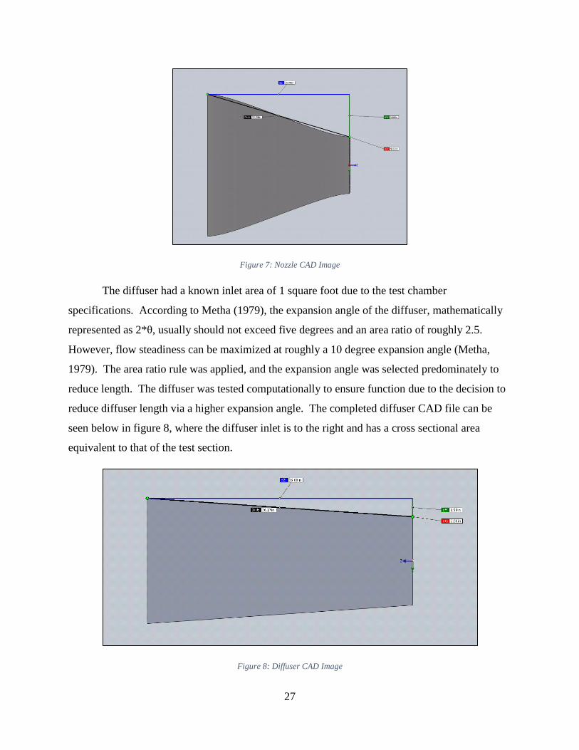
The diffuser had a known inlet area of 1 square foot due to the test chamber

specifications. According to Metha (1979), the expansion angle of the diffuser, mathematically

represented as 2*θ, usually should not exceed five degrees and an area ratio of roughly 2.5.

However, flow steadiness can be maximized at roughly a 10 degree expansion angle (Metha,

1979). The area ratio rule was applied, and the expansion angle was selected predominately to

reduce length. The diffuser was tested computationally to ensure function due to the decision to

reduce diffuser length via a higher expansion angle. The completed diffuser CAD file can be

seen below in figure 8, where the diffuser inlet is to the right and has a cross sectional area

equivalent to that of the test section.

Figure 8: Diffuser CAD Image

28

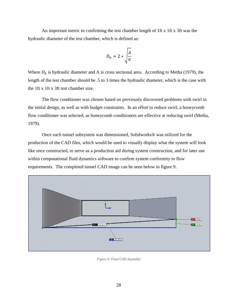
An important metric in confirming the test chamber length of 1ft x 1ft x 3ft was the

hydraulic diameter of the test chamber, which is defined as:

𝐷ℎ = 2 ∗ √𝐴

𝜋

Where 𝐷ℎ is hydraulic diameter and A is cross sectional area. According to Metha (1979), the

length of the test chamber should be .5 to 3 times the hydraulic diameter, which is the case with

the 1ft x 1ft x 3ft test chamber size.

The flow conditioner was chosen based on previously discovered problems with swirl in

the initial design, as well as with budget constraints. In an effort to reduce swirl, a honeycomb

flow conditioner was selected, as honeycomb conditioners are effective at reducing swirl (Metha,

1979).

Once each tunnel subsystem was dimensioned, Solidworks® was utilized for the

production of the CAD files, which would be used to visually display what the system will look

like once constructed, to serve as a production aid during system construction, and for later use

within computational fluid dynamics software to confirm system conformity to flow

requirements. The completed tunnel CAD image can be seen below in figure 9.

Figure 9: Final CAD Assembly

29

3.1.4 Computational Testing

In order to confirm that the system design behaved appropriately concerning airflow,

particularly regarding air velocity and turbulence within the test chamber, ANSYS® Fluent®

was utilized. The Solidworks® CAD file was exported as an .IGS file and imported into

Fluent®. The full Fluent® report, which includes data on boundary conditions, mesh, and setup

inputs for the final CFD iteration, can be found in appendix F. Figure 10, shown below, depicts

vorticity results through the three dimensional tunnel.

Figure 10: Three Dimensional Vorticity Simulation

In order to lower simulation time, and to minimize human error in ANSYS® setup, a

two-dimensional approximation was made regarding flow through the tunnel using ANSYS®

Design Modeler®. It is important to note, however, that the 2D approximation does not include

a honeycomb flow conditioner, and so results have potential to display a less uniform flow

profile than the physical system produces.

30

Figure 11: Velocity vs Distance

After the simulation had been set up with the known boundary conditions and fan speed

at the end of the diffuser, the simulation ran for 1500 iterations, which was comfortably past the

threshold of solution convergence. Figure 11 and figure 12 show the velocity profile and

pressure profile of the tunnel over distance from the nozzle respectively. It is evident that the

highest velocities occur in the test chamber, and succeed in meeting the minimum velocity set

forth in the functional requirements and design parameters.

31

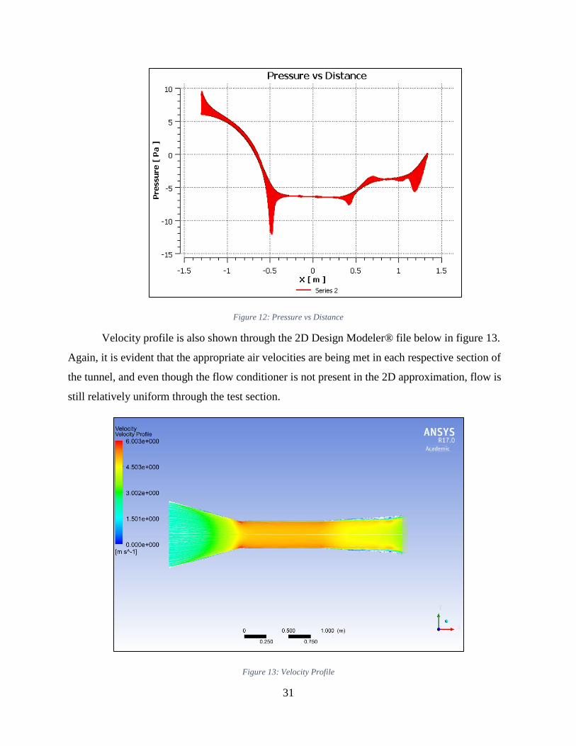
Figure 12: Pressure vs Distance

Velocity profile is also shown through the 2D Design Modeler® file below in figure 13.

Again, it is evident that the appropriate air velocities are being met in each respective section of

the tunnel, and even though the flow conditioner is not present in the 2D approximation, flow is

still relatively uniform through the test section.

Figure 13: Velocity Profile

32

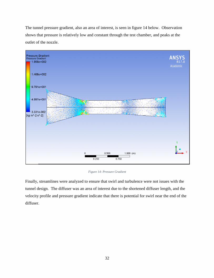
The tunnel pressure gradient, also an area of interest, is seen in figure 14 below. Observation

shows that pressure is relatively low and constant through the test chamber, and peaks at the

outlet of the nozzle.

Figure 14: Pressure Gradient

Finally, streamlines were analyzed to ensure that swirl and turbulence were not issues with the

tunnel design. The diffuser was an area of interest due to the shortened diffuser length, and the

velocity profile and pressure gradient indicate that there is potential for swirl near the end of the

diffuser.

33

Figure 15: Turbulence Check

Figure 15 confirms that there is potential swirl near the end of the diffuser. However, as it is

minimal, and thus likely does not have a significant detriment on the quality of flow within the

test section, the shortened diffuser length in the interest of saving space could be deemed safe for

this tunnels purpose.

3.1.5 Design Limitations

Given the functional requirements and design parameters that limit system size, noise

generation, and ambient condition alteration, this tunnel has predictable limitations in the types

of configurations that can be tested, as well as the velocity range a given configuration can be

tested over. It is also the case that, based on the heating element used to heat geometry, as well

as the presence and accuracy of selected instrumentation, that additional design limitations will

be generated.

34

Computational test results indicate a maximum velocity between 5 and 5.5 meters per

second, which is the first and most clear limitation of the tunnel. This makes any tests involving

components exposed to higher speeds, such as automotive or aerospace components, or even

components exposed to higher speed winds during storms or other natural sources, impossible to

test. However, experimental data collected with this tunnel system can be trended to gain a sense

of how the heat transfer coefficient will behave at air velocities close to the maximum tunnel

speed.

Additionally, in respect to airflow, only laminar flow environments can be tested. Of

course, realistically, not all flow that could be experienced by a geometry in practice is laminar.

However, by testing laminar flow, it is possible to experimentally obtain a potential lower bound

on the convective heat transfer of the test configuration for that flow environment, as laminar

flow is less effective at forced convective heat transfer than turbulent flow (Patil, 2015).

In respect to instrumentation, the most readily apparent limitation is the accuracy and

precision of the instruments themselves. Factors such as signal noise and general lack of

accuracy to a high degree contribute to data acquisition limitation. It is also worth mentioning

that, if uninsulated, the thermocouples themselves can potentially act as a heat sink, and thus can

detract from the accuracy of the configuration surface temperature measurements.

Finally, the system heating element surface area is roughly 0.04129 m2. Due to the

inherent requirement for heat to be transferred to the geometry via conduction, tested

configurations must be sized around to the size of the heating element. Insulation may also need

to be adjusted depending upon the given test configuration.

3.2 Measurement and Instrumentation

This heat transfer demonstration device consists of various sub-systems that put together

are capable of making room temperature airflow through the device and quickly heating it up

through the test chamber. Most sub-systems are responsible for providing the conditions at which

the convective heat transfer coefficient is found. For instance, the fan, diffuser and nozzle are

responsible for the laminar air that goes into the test chamber, whereas the power generation sub-

system and the heated plate are responsible for the heating of air. Yet, none of these portions of

the project are really responsible for the measurement of ‘h’, the convective heat transfer

35

coefficient. A separate sub-system is required to measure the temperature of air and its velocity

through the test chamber. These measurements are done by the instrumentation sub-system.

The instrumentation sub-system consists of the measurement tools and the LabVIEW

program. The measurement tools consist of thermocouples and anemometers. These are simple

and cheap devices that can be easily connected to the LabVIEW program. The computer

software, LabVIEW, plays a major role in this project. In order for the experiments to have

results in real-time, LabVIEW is required to continuously calibrate measurements and run

calculations to find the value of ‘h’. This section of the report deals with the instruments used to

measure physical quantities in the test chamber and the software logic used to calculate the

convective heat transfer coefficient.

3.2.1 Thermocouples

Thermocouples are temperature sensing devices that consist of two different types of

metal wires welded together to produce small voltage differentials. These differentials occur due

to the Seebeck Effect, which describes the continuous current flow in two connected wires of

distinct metals. They can be measured and calibrated in order to electronically determine the

temperature of surfaces and fluids.

There are different types of thermocouples. Each of the thermocouple types are

distinguished by their temperature range and their sensitivity. Table 1 details thermocouples’

temperature range and sensitivity. It is clear from the table that some thermocouples have better

sensitivity and better temperature ranges. According to OMEGA, a global leader in the

production of thermal sensors and other components, type K thermocouples are considered a

multipurpose thermocouple due its large temperature range and low cost. Since this project deals

with a fairly high temperature scale, it has been decided that type K thermocouples are the most

applicable for large variations in temperature, such as the hot plate. Type T thermocouples are

more accurate are more adequate for the measurement of the temperature of air or temperatures

surrounding the plate. The protection cover of type T thermocouples is also different from that of

K parts. T-type cover cannot withstand the temperature range of the experiments and therefore it

must be safely positioned within the test chamber such that the heat of the plate does not

overheat the device.

36

Table 1: Thermocouple Types

Thermocouple Type Temperature Range (°C) Standard Limits of Error (°C)

J 0 to 750 2.2

K -200 to 1250 2.2

E -200 to 900 1.7

T -250 to 350 1.0

In total, this device uses seven thermocouples. Three of which are T-type and the other

four, K-type. The schematic for this setup is depicted in Figure 16, where the green box is the

test chamber and the gray box is the hot plate. Here, the letters T and K represent the type of the

thermocouple used and its position on the plate or test chamber. Also, notice that every single

thermocouple is labeled from T0 to T6. This setup was chosen in order to compare measured

temperatures at the center of plate as well as the edges of the plate. The T thermocouples were

lined up with the K thermocouples to ensure the temperature differential is calculated in the

direction of airflow. Thus, there are four ΔT’s: ΔT3 = T3 – T0; ΔT4 = T4 – T1; ΔT5 = T5 – T1;

ΔT6 = T6 – T2. These temperature differentials are used to calculate the convective heat transfer

coefficient.

Figure 16: Thermocouples positioned according to letter type

37

3.2.2 Hot-Wire Anemometer

Anemometers are devices used to measure wind speed. Anemometers were primarily

used for meteorological purposes and were gradually refined in both technology and application.

The mechanical design of anemometers includes simple cup anemometers and windmill

anemometers. Both of these anemometers use the wind speed to rotate a fan. Yet, cup

anemometers rotate in the direction tangent to the wind vector, whereas windmill anemometers

rotate orthogonally to the wind. Both of these can be connected to analog gauges to measure the

speed of wind.

Hot-wire anemometers use a finer technology to accurately measure the velocity of air.

They are part of a segment of anemometers commonly known as thermal anemometers and are

mostly used in laminar to transition flow types. Hot-wire anemometers use a filament of wire

that is kept at constant temperature due to a self-regulatory current through the wire filament.

Once wind blows over the hot wire, it changes the temperature of the wire, which, through

several internal flow calculations, determines the speed of air. Due to their high accuracy even in

large air velocity ranges and their rather quick response, these devices are found in industrial

applications.

The hot-wire anemometer, Testo 405i, was selected for this project (see Appendix B).

Among other hot-wire anemometers, this was the most cost-effective solution for it uses a

smartphone application to display its measurements. Even though this device is also used in

industrial applications, it is significantly cheaper than other devices that have similar operations.

It measures temperature and air velocity simultaneously and is capable of exporting all data in

multiple formats!

3.2.3 LabVIEW and DAQ Box

While the thermocouples and the hot-wire anemometer deal with measurement of

specific physical variables, the LabVIEW program and the Data Acquisition (DAQ) Box are

responsible for converting the electric pulses from the physical channels into digital data. The

DAQ Box (model NI-USB-6363) receives analog voltage variations from the thermocouples and

uses its internal analog-to-digital converter to transform the analog voltage impulses into bits. It

38

is a 16-bit device with a maximum dynamic range of +/- 10V. Thus, the resolution is

approximately 305.2µV/bit.

The LabVIEW program runs the data collection in this project. It is responsible for

collecting the signal from the DAQ Box as well as running the program that calculates the heat

transfer coefficient and outputting all of the data into excel files. The LabVIEW runs an endless

while loop, which can only be stopped manually. This loop will continuously gather data from

each thermocouple individually through a stacked sequence structure shown in Figure 17. Next,

it will run data gathered from the thermocouples back into the loop in order to perform the

calculation of four separate heat transfer coefficients. This feedback system and the calculation

of the coefficient is depicted in Figure 18. Notice that, for the equation, two indicators are used

for ‘Power’ and ‘Area’ and that the temperature for other thermocouples is fed back into the

system after being delayed in time. This means that the orange symbol with an arrow represents

a Z-transform, which means that the output is fed back into the system, but delayed one unit in

time. This was used to internally calculate the heat transfer coefficient. Finally, Figure 19 details

the portion of the block diagram in which the output is written to an excel file. Data is written to

the excel file according to a delay time variable that is determined by the user.

Figure 17: Frame of one stacked sequence gathering data for one thermocouple

39

Figure 18: Calculation of the heat transfer coefficient in the LabVIEW program

Figure 19: Write-to-file and tab labels on block diagram

For closer view of the front panel of the LabVIEW program and the file while running,

please see Appendix C.

40

3.3 Experimentation

In order to analyze the behavior of the convective heat transfer coefficient, a Design of

Experiments was created to describe each experiment that our team would conduct. This section

will discuss the set up and procedures involved in each of these experiments. The following are

an explanation of each operation, a recommendation for future investigation, and an examination

of possible sources of error. Appendix B has photos of the instrumentation and setup used to

conducted experiments.

3.3.1 Circuit Configuration

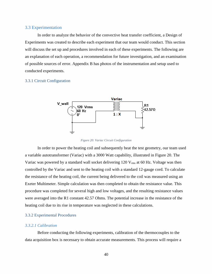
Figure 20: Variac Circuit Configuration

In order to power the heating coil and subsequently heat the test geometry, our team used

a variable autotransformer (Variac) with a 3000 Watt capability, illustrated in Figure 20. The

Variac was powered by a standard wall socket delivering 120 Vrms at 60 Hz. Voltage was then

controlled by the Variac and sent to the heating coil with a standard 12-gauge cord. To calculate

the resistance of the heating coil, the current being delivered to the coil was measured using an

Exeter Multimeter. Simple calculation was then completed to obtain the resistance value. This

procedure was completed for several high and low voltages, and the resulting resistance values

were averaged into the R1 constant 42.57 Ohms. The potential increase in the resistance of the

heating coil due to its rise in temperature was neglected in these calculations.

3.3.2 Experimental Procedures

3.3.2.1 Calibration

Before conducting the following experiments, calibration of the thermocouples to the

data acquisition box is necessary to obtain accurate measurements. This process will require a

41

previously calibrated thermocouple and a multimeter. The steps to complete the calibration are as

follows:

1. Fasten calibrated thermocouple onto test geometry and connect it to the multimeter.

2. Set variac to 100V and allow the temperature of the test geometry to rise to

approximately 250C.

3. Input correctly measured power into LabVIEW.

4. Once the temperature of the plate has reached steady state, input the temperature reading

from the multimeter into LabVIEW.

5. Record approximately 10 data points in LabVIEW at 0 m/s.

6. Using the fan controller, increase the air velocity by .5 m/s.

7. Wait for the plate temperature to reach steady state again and input the temperature

reading from the multimeter into LabVIEW.

8. Record approximately 10 data points in LabVIEW.

9. Repeat steps 5-8 until maximum fan speed is reached.

10. Once the tests are completed, stop the program and open the excel file containing the

recorded data.

11. Create a scatterplot of the data with Input Temperature on the x-axis and Thermocouple

#3 on the y-axis. Add a trend line to the graph and show the equation as well as the R2

value. Record the slope and intercept of each plot equation.

12. Repeat step 8 for Thermocouple #4, #5, and #6.

13. Plug the slope and intercept of each corresponding thermocouple into the front panel of

the LabVIEW program.

14. Be sure to Make Current Values Default under the Edit menu and save the program.

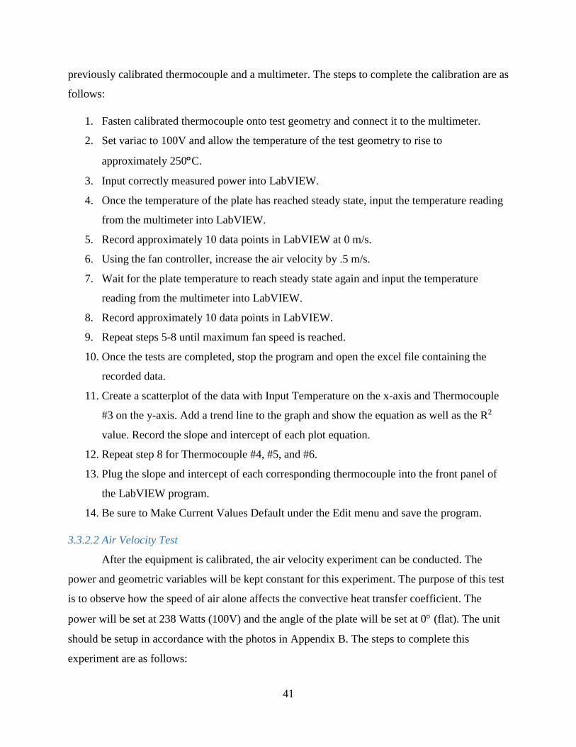
3.3.2.2 Air Velocity Test

After the equipment is calibrated, the air velocity experiment can be conducted. The

power and geometric variables will be kept constant for this experiment. The purpose of this test

is to observe how the speed of air alone affects the convective heat transfer coefficient. The

power will be set at 238 Watts (100V) and the angle of the plate will be set at 0 (flat). The unit

should be setup in accordance with the photos in Appendix B. The steps to complete this

experiment are as follows:

42

1. Set variac to 100V.

2. Allow temperature of test geometry to rise to roughly 250C (approximately 20 minutes).

3. Once the temperature of the plate has reached steady state, set air velocity at 0 m/s and

record approximately 10 data points in LabVIEW.

4. Increase the air velocity by .5 m/s using the fan controller and wait for the plate

temperature to reach steady state again. Record approximately 10 data points in

LabVIEW.

5. Repeat step 4 until the maximum fan speed is reached, leaving the LabVIEW program

running continuously during the experiment.

This experiment can be expanded to include data at different power levels and geometric

configurations to compare how ‘h’ values are affected. More precise measurements could be

taken using smaller incremental increases to improve the accuracy of the experiment.

3.3.2.3 Natural Convection Test

Our device is also capable of measuring the convective heat transfer coefficient for

natural convection. To simulate a natural convective environment, air velocity was set to 0 m/s,

the geometric configuration remains constant, and the glass top of the test chamber is removed

throughout the duration of the experiment. Plate temperature is increased in linear increments by

increasing the input Power. The steps to complete this experiment are as follows:

1. To simulate ambient air, remove the top glass from the test chamber.

2. Set the variac to 50V and wait for the temperature of the plate to stabilize.

3. Record approximately 10 data points in the LabVIEW program.

4. Repeat step 2 and 3 for 60V, 70V, 80V, 90V, and 100V.

This experiment can be expanded to include data at different input power levels. More precise

measurements could be taken by increasing the number of input voltages at which data points are

recorded.

After the data collected in this experiment was analyzed, it was decided that the results

were inconclusive. Possible causes of the flawed data were hypothesized when reviewing the

experimental procedures. Although the top glass of the test chamber was removed, the side glass

pieces remained in place, which could have diminished the authenticity of a naturally convective

43

environment. The experiment was not conducted in an air tight environment; thus possible

external movements of air could have affected the natural convection process. Conjecture was

also made that the instrumentation used, specifically the thermocouples, may not have been

correctly calibrated for this experiment, or were not functioning properly during the test. In

future experiments, it is the recommendation of this team that stricter measures be taken to

simulate a naturally convective climate, and the thermocouples be recalibrated and tested before

the experiment is conducted.

3.3.2.4 Geometry Orientation Test

The geometric configuration tests were completed in a similar fashion to the air velocity

tests. At each geometric configuration, the plate was heated to roughly 250C and air was drawn

through the test chamber at increasing velocities. The test geometry used in this experiment was

mounted to an adjustable base stand so that the angle of the plate could be increased. The steps to

complete this experiment are as follows:

0 Plate Angle

1. Remove the top of the test chamber and set the test plate’s angle at 0 to the bottom of

test chamber. The plate should be in its resting, flat position.

2. Replace the glass top of the test chamber, and ensure a good seal is made between the

silicon and the glass.

3. Set the variac at 100V and allow the temperature of the test geometry to rise to roughly

250C (approximately 20 minutes).

4. Once the temperature of the plate has reached steady state, set air velocity at 0 m/s.

Record approximately 10 data points in LabVIEW.

5. Record approximately 10 data points in LabVIEW at 0 m/s.

6. Using the fan controller, increase the air velocity by .5 m/s.

7. Wait for the plate temperature to reach steady state again and input the temperature

reading from the multimeter into LabVIEW.

8. Record approximately 10 data points in LabVIEW.

9. Repeat steps 5-8 until maximum fan speed is reached, leaving the LabVIEW program

running continuously during the experiment.

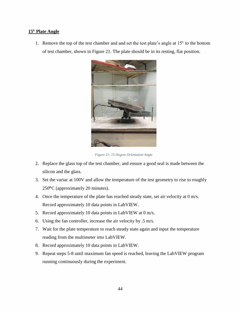
44

15 Plate Angle

1. Remove the top of the test chamber and and set the test plate’s angle at 15 to the bottom

of test chamber, shown in Figure 21. The plate should be in its resting, flat position.

Figure 21: 15 Degree Orientation Angle

2. Replace the glass top of the test chamber, and ensure a good seal is made between the

silicon and the glass.

3. Set the variac at 100V and allow the temperature of the test geometry to rise to roughly

250C (approximately 20 minutes).

4. Once the temperature of the plate has reached steady state, set air velocity at 0 m/s.

Record approximately 10 data points in LabVIEW.

5. Record approximately 10 data points in LabVIEW at 0 m/s.

6. Using the fan controller, increase the air velocity by .5 m/s.

7. Wait for the plate temperature to reach steady state again and input the temperature

reading from the multimeter into LabVIEW.

8. Record approximately 10 data points in LabVIEW.

9. Repeat steps 5-8 until maximum fan speed is reached, leaving the LabVIEW program

running continuously during the experiment.

45

30 Plate Angle

1. Remove the top of the test chamber and and set the test plate’s angle at 30 to the bottom

of test chamber, shown in Figure 22. The plate should be in its resting, flat position.

Figure 22: 30 Degree Orientation Angle

2. Replace the glass top of the test chamber, and ensure a good seal is made between the

silicon and the glass.

3. Set the variac at 100V and allow the temperature of the test geometry to rise to roughly

250C

(approximately 20 minutes).

4. Once the temperature of the plate has reached steady state, set air velocity at 0 m/s.

Record approximately 10 data points in LabVIEW.

5. Record approximately 10 data points in LabVIEW at 0 m/s.

6. Using the fan controller, increase the air velocity by .5 m/s.

7. Wait for the plate temperature to reach steady state again and input the temperature

reading from the multimeter into LabVIEW.

8. Record approximately 10 data points in LabVIEW.

9. Repeat steps 5-8 until maximum fan speed is reached, leaving the LabVIEW program

running continuously during the experiment.

This experiment has many opportunities for expansion. This experiment could be conducted

again at different Power levels to observe the rate at which the ‘h’ value changes at higher

46

and lower temperatures. The current base mount is only adjustable up to 30. In future

experiments, a different mounting mechanism could allow a fuller range of motion so that all

angles through 90 could be tested. Cylindrical, spherical and prismatic geometries could

also be configured into this device and tested at different geometric orientations.

3.3.2.5 Textbook Sample Problem

Problems such as the one shown in Figure 27 could be actively demonstrated in class.

After theoretical calculation is performed, students can compare their calculated values to the

ones obtained through experimentation using this device. Please reference Appendix G for a

detailed sample problem that can be tested using the demonstration unit.

47

Chapter 4: Results and Analysis

The following section will outline the results from numerous data collection experiments

conducted using the heat transfer demonstration unit constructed by our team. Comparisons

between MATLAB predictions and experiment results are shown and discussed in the following

section. Additional graphs, charts, and discussion can be found in Appendix D and Appendix E.

4.1 MATLAB Prediction and Experimental Result for ΔT vs. Power

Figure 23 shows one of the predictions done at the early stages of this project. It

explicitly depicts the linear relationship between the temperature differential, ΔT, and power.

The slope comes from the equation, �̇� = ℎ𝐴∆𝑇, where the heat transfer coefficient and the area

of the plate, determine that slope. Since this experiment was done with wind blown over the

plate, the heat transfer equation for forced convection and laminar flow was implemented.

Further, since the Prandtl number for air at room temperature is 0.713, the equation for the

average Nusselt number was: 𝑁𝑢̅̅ ̅̅ = 0.664√𝑅𝑒 ∗ √𝑃𝑟3

Here, Re stands for the Reynold’s number. The Reynold’s number is defined by: 𝑅𝑒 = 𝑣∗𝐷

𝜐.

Here, v is the velocity, D is the hydraulic diameter, υ is the kinematic viscosity. Finally, h is

defined by: ℎ = 𝑘𝑁𝑢̅̅ ̅̅

𝐿, where k is thermal conductivity of air, 𝑁𝑢̅̅ ̅̅ is the average Nusselt number

on the plate. Once all of the values were determine, the air velocity was set from 0.5 to 4 m/s in

increments of 0.5 m/s in order to define 8 distinct plots. Figure 23 also shows a dashed line at

fixed power. That line represents the maximum power that could be reached in this project’s

setup. ΔT was set as the independent variable linearly growing from 0 to 450 K.

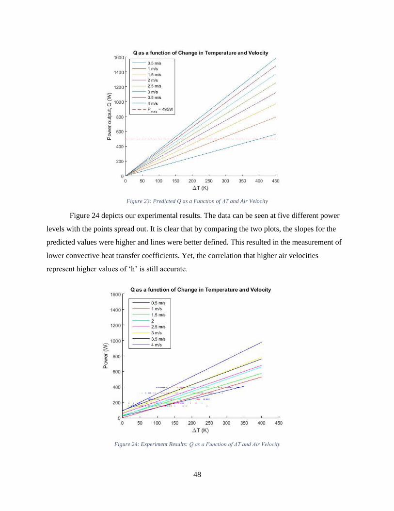
48

Figure 23: Predicted Q as a Function of ΔT and Air Velocity

Figure 24 depicts our experimental results. The data can be seen at five different power

levels with the points spread out. It is clear that by comparing the two plots, the slopes for the

predicted values were higher and lines were better defined. This resulted in the measurement of

lower convective heat transfer coefficients. Yet, the correlation that higher air velocities

represent higher values of ‘h’ is still accurate.

Figure 24: Experiment Results: Q as a Function of ΔT and Air Velocity

49

4.2 MATLAB Prediction vs. Experimental Data

Figure 25: At left, predicted ΔT vs. ‘h’. At right, Experimental data ΔT vs. ‘h’.

Figure 25 left was generated through a MATLAB script. It is the prediction for a

correlation between the convective heat transfer coefficient and the temperature differential. The

five separate curves correspond to five different power inputs at 150W, 190W, 238W, 318W and

392W. These values correspond to the ones in Figure 25 right, which represents the results from

experiments of different air velocities. These two plots were calculated separately, but they

clearly represent the same curves and equation, �̇� = ℎ𝐴∆𝑇. Thus, Figure 26 superimposes both

plots. It is clear that the experimental data is spot on the predicted plots. This serves as proof the

LabVIEW program is correct and has used the right equation to determine the heat transfer

coefficient.

Figure 26: Experimental data ΔT vs. ‘h’ superimposed onto predicted ΔT vs. ‘h’

50

4.3 Plate Orientation Angle Experiment

A significant experiment conducted by our team included testing for the heat transfer

coefficient at different plate orientation angles. The tests included ‘h’ measurements at 0, 15, and

30 degrees of elevation while varying air velocity over the plate, reference chapter 3 for more

information about the test procedure. Figure 27 displays the results of orientation testing. The

heat transfer coefficient is shown to increase with increasing plate orientation angles; therefore,

the highest values of ‘h’ are seen to occur with steeper geometric orientations. It can be seen that

higher values of ‘h’ translate to higher rates of heat transfer. This is because, at a constant heat

flux, changes in temperature must be smaller to accommodate large ‘h’ values. Thus, surface

temperature of the test configuration is more comparable to that of the configuration’s

surroundings when higher ‘h’ values are present. Figure 27 presents data from thermocouple

number four on the unit, and the graphs from the other thermocouples can be found in Appendix

E.

Figure 27: 'h' as a Function of Air Velocity

51

4.4 Power vs. Heat Transfer Coefficient Experiment

Figure 28, displays the heat transfer coefficient as a function of air velocity and power.

The goal of the experiment was to determine the relationship between ‘h’ and the power input

into the test. Since all curves are intertwined, power does not affect the heat transfer coefficient.

There is not an increasing or decreasing correlation between input power and the determination

of ‘h’. The input power directly influences the surface temperature of plate, thus proving the

increasing surface temperature does not influence the heat transfer coefficient, assuming other

variables remain constant between power experiments.

Figure 28: 'h' as a Function of Air Velocity and Power

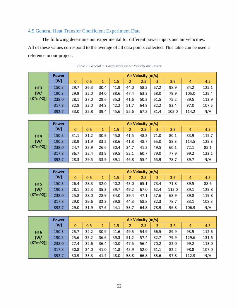
52

4.5 General Heat Transfer Coefficient Experiment Data

The following determine our experimental for different power inputs and air velocities.

All of these values correspond to the average of all data points collected. This table can be used a

reference in our project.

Table 2: General 'h' Coefficients for Air Velocity and Power

HT3 [W/

(K*m^2)]

Power [W]

Air Velocity [m/s]

0 0.5 1 1.5 2 2.5 3 3.5 4 4.5

150.3 29.7 26.3 30.4 41.9 44.0 58.3 67.2 98.9 84.2 125.1

190.3 29.9 32.0 34.0 38.6 47.4 63.3 68.0 79.9 105.0 125.4

238.0 28.1 27.0 29.6 35.3 41.6 50.2 61.5 75.2 89.5 112.9

317.8 32.8 33.0 34.8 42.2 51.7 64.9 82.2 82.4 97.0 107.5

392.7 33.0 32.8 39.4 45.6 55.6 67.3 81.4 103.0 114.2 N/A

HT4 [W/

(K*m^2)]

Power [W]

Air Velocity [m/s]

0 0.5 1 1.5 2 2.5 3 3.5 4 4.5

150.3 31.1 31.2 30.9 45.8 41.5 48.3 71.0 80.1 83.9 115.7

190.3 28.9 31.9 33.2 38.6 41.8 48.7 65.0 88.3 114.5 125.3

238.0 24.7 23.9 26.6 30.4 34.7 41.3 49.5 60.1 72.1 85.1

317.8 36.7 32.4 33.9 39.5 52.1 60.7 79.0 77.9 99.2 123.1

392.7 28.3 29.5 33.9 39.1 46.8 55.4 65.9 78.7 89.7 N/A

HT5 [W/

(K*m^2)]

Power [W]

Air Velocity [m/s]

0 0.5 1 1.5 2 2.5 3 3.5 4 4.5

150.3 26.4 28.3 32.0 40.2 43.0 65.1 73.4 71.8 89.5 88.6

190.3 28.1 32.3 35.3 39.7 49.2 67.0 62.4 115.0 89.1 125.8

238.0 25.8 28.0 28.9 34.0 39.4 47.1 57.6 68.9 89.8 119.8

317.8 29.0 29.6 32.3 39.8 44.3 58.8 82.3 78.7 83.1 108.3

392.7 29.0 31.9 37.6 44.1 53.7 64.8 78.9 96.8 106.9 N/A

HT6 [W/

(K*m^2)]

Power [W]

Air Velocity [m/s]

0 0.5 1 1.5 2 2.5 3 3.5 4 4.5

150.3 25.7 32.2 30.9 41.6 49.5 54.9 66.5 89.9 93.5 112.6

190.3 25.6 33.2 36.6 39.3 51.2 57.4 82.7 79.9 129.6 131.6

238.0 27.4 32.6 36.4 40.0 47.5 56.4 70.2 82.0 99.2 113.0

317.8 30.8 34.0 41.0 41.8 45.9 52.0 61.1 82.2 98.8 107.0

392.7 30.9 35.3 41.7 48.0 58.8 66.8 85.6 97.8 112.9 N/A

53

4.6 Possible Sources of Experimental Error

One possible source of error could be the measurements from the DAQ box. As

mentioned in the Instrumentation section, the DAQ box has a resolution of approximately

305µV/bit. This seems like a high resolution for many instruments. However, voltage

differentials produced by thermocouples are very small in the order of tens of millivolts per

degree Celsius. In fact, on the National Instruments website, one can find the voltage output, in

millivolts, of K-type thermocouples for various temperatures. Since in this project we are not

dealing with temperatures lower than 0°C and higher than 400°C, the linear resolution for this

type of thermocouple would be 16.397𝑚𝑉−0𝑚𝑉

400°C−0°C= 40.993

𝜇𝑉

°C. 16.397mV represents the output

voltage differential at 400°C and 0mV, at 0°C. Comparing the resolution of the DAQ Box to

that of the thermocouple would lead to 305

𝜇𝑉

𝑏𝑖𝑡

40.993𝜇𝑉

℃

= 7.44℃

𝑏𝑖𝑡. Finally, this means that every bit in

the DAQ Box would only measure differences in quantities of 7.44°C for K-type thermocouples.

This lack of accurate measurements could be a source of error in the data.

During the construction of this device, thermocouples were pushed through a small from

the bottom of the wind tunnel into the test chamber. This could have damaged the metal wires

that create the small voltage differentials. Also, the thermocouples were positioned such that the

welded ball touches the hot plate. Yet, high temperature thermal pastes could glue the

thermocouples to the plate and provide better readings for the thermocouples. Further, due to

their placement, thermocouples are not insulated from air. This could cause the wires of the

thermocouple to act as a heat sink, consequently leading to bad readings from the thermocouples.

54

Chapter 5: Conclusion and Recommendations

After design, construction, and experimentation of our project, the demonstration device

is now capable of measuring the convective heat transfer coefficient ‘h’. Due to its portability it

can be easily set up and used in a classroom as a visual aid. Our team’s attention to detail and

professional level of craftsmanship has made the device a reliable source of data acquisition that

will remain functional for years to come. Through our team’s own design of experiments, we

began investigating the relationship between the geometry, air flow, and the convective heat

transfer coefficient.

As predicted in Chapter 3, the faster air is blown across the test geometry the more heat

will be transferred between the two mediums, and thus, the cooler the plate will become. And

because higher rates of heat transfer correspond to higher values of ‘h’, it follows that as air

velocity increases, ‘h’ also increases. Figure 24 shows the linear correlation between the air

velocity and the temperature of the plate.

From the results our team collected, a relationship between the convective heat transfer

coefficient and geometric orientation can be interpreted. The analysis of gathered data

determined that steeper slopes in the test geometry correspond to higher rates of heat transfer and

thusly higher values of ‘h’. In future experiments, different mounting mechanisms could allow a

fuller range of motion so that all angles through 90 could be tested. Cylindrical, spherical and

prismatic geometries could also be mounted into this device and tested at different geometric

orientations.

55

References

Awuah, G. B., Ramaswamy, H. S., & Simpson, B. K. (1995). Comparison of two methods for

evaluating fluid-to-surface heat transfer coefficients. Food Research International, 28(3), 261-

271. Retrieved November 23, 2015.

Baals, Donald D., and William R. Corliss. Wind Tunnels of NASA. Washington, D.C.: Scientific

and Technical Information Branch, National Aeronautics and Space Administration, 1981. Print.

Bergman, T. L., Lavine, A. S., Incropera, F. P., & Dewitt, D. P. (2007). Fundamentals of Heat

and Mass Transfer (7th ed.). Hoboken, NJ: John Wiley.

Bonwell, C. C., & Eison, J. A. (1991). Active Learning: Creating Excitement in the

Classroom (Rep. No. ED 336 049). Washington, DC: ERIC Clearinghouse on Higher Education.

doi:ASHE-ERIC Higher Education Report. U.S. Department of Education

CDC/NIOSH. Noise and Hearing Loss Prevention. Cincinnati, OH: U.S. Department of Health

and Human Services; 1998.

Cuesta, F. J., Lamúa, M., & Alique, R. (2012). A new exact numerical series for the

determination of the Biot number: Application for the inverse estimation of the surface heat

transfer coefficient in food processing. International Journal of Heat and Mass Transfer, 55(15-

16), 4053-4062. doi:10.1016/j.ijheatmasstransfer.2012.03.047

Dunbar, Brian. "What Are Wind Tunnels?" NASA. NASA, 24 June 2014. Web.

Fokaides, P. A., & Kalogirou, S. A. (2011). Application of infrared thermography for the

determination of the overall heat transfer coefficient (U-Value) in building envelopes. Applied

Energy, 88(12), 4358-4365. doi:10.1016/j.apenergy.2011.05.014

Gallagher, J. E. (2005, May 11). The Effects of Flow Conditioning. Retrieved February 24, 2016,

from http://www.wwdmag.com/flow-metering/effects-flow-conditioning

Guo, Z., Xiong, S., Liu, B. C., Li, M., & Allison, J. (2009). Determination of the metal/die

interfacial heat transfer coefficient and its application in evaluating the pressure distribution

inside the casting during the high pressure die casting process. International Journal of Cast

Metals Research, 22(1-4), 327-330. doi:10.1179/136404609x368109

Hake, R. R. (1998). Interactive-engagement versus traditional methods: A six-thousand-student

survey of mechanics test data for introductory physics courses. Am. J. Phys. American Journal of

Physics, 66(1), 64. doi:10.1119/1.18809

Kirby, Mark S., and John Hansman. "EXPERIMENTAL MEASUREMENTS OF HEAT

TRANSFER FROM AN ICED SURFACE DURING ARTIFICIAL AND NATURAL CLOUD

ICING CONDITIONS." (n.d.): n. pag. NASA.gov. Web.

56

Metha R. D., Bradshaw P. “Design Rules for Small Low Speed Wind Tunnels” Journal of Royal

Aeronautical Society 1979, Vol. 73

Pate, M. B. (2008). An active learning approach for teaching undergraduate heat transfer. In

2008 Proceedings of the ASME Summer Heat Transfer Conference (Vol. 3, pp. 677-683).

ASME.

Patil, Pranit M., Amol P. Yadav, and P. A. Patil, Dr. "Comparative Study between Heat Transfer

through Laminar Flow and Turbulent Flow." International Journal of Innovative Research in

Science, Engineering and Technology 4.4 (2015): n. pag. Web.

Suh, Nam P. The Principles of Design. New York: Oxford UP, 1990. Print.

Tables of Thermoelectric Voltages for All Thermocouple Types. (n.d.). Retrieved April 20,

2016, from http://www.ni.com/white-paper/4231/en/#toc2

Tan, F. L., & Fok, S. C. (2008). Development of interactive learning activities in heat

transfer. World Review of Science, Technology and Sustainable Development, 5(3-4), 354-372.

Retrieved January 14, 2016.

"Thermal Wind Tunnel." Audi Wind Tunnels AUDI AG. N.p., n.d. Web.Kumar, A., and N.

Barthakur. "Convective Heat Transfer Measurements of Plants in a Wind Tunnel." Springer

Link. Kluwer Academic Publishers, Dec. 1971.

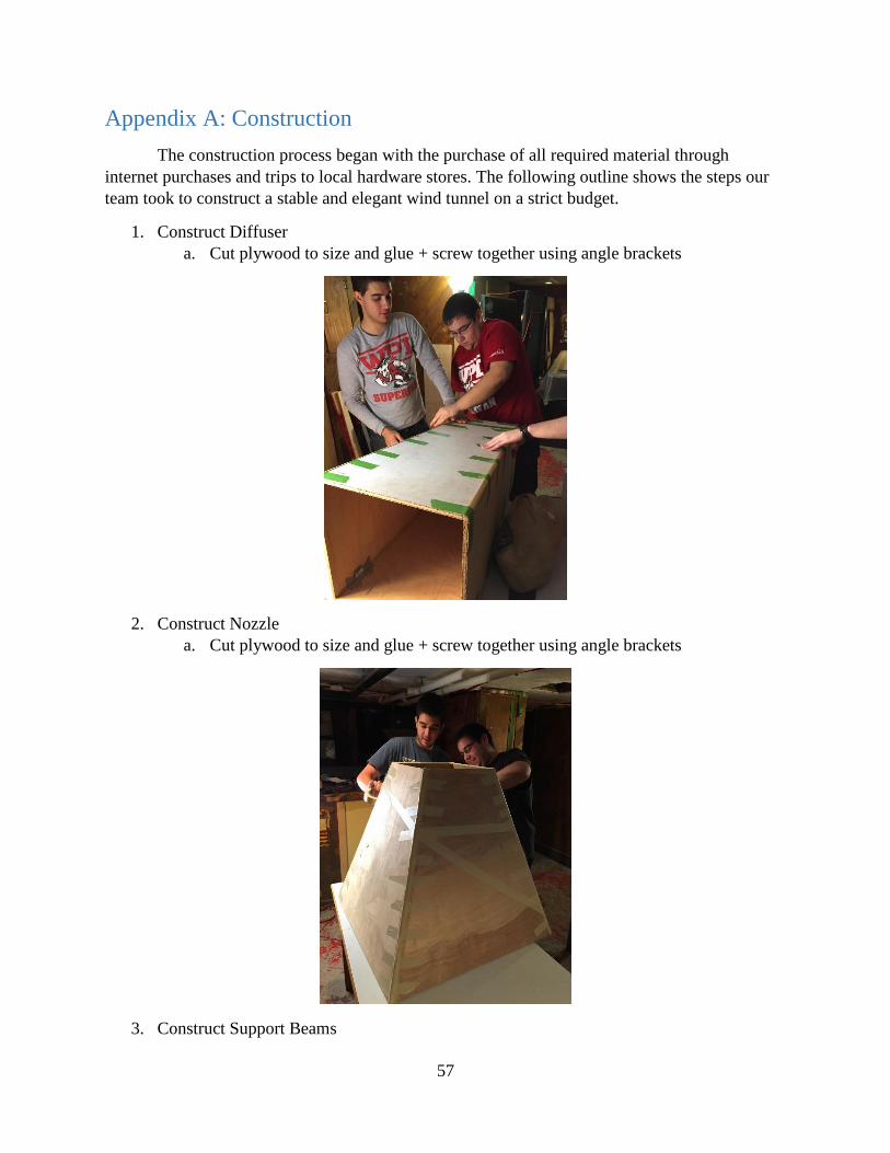
57

Appendix A: Construction

The construction process began with the purchase of all required material through

internet purchases and trips to local hardware stores. The following outline shows the steps our

team took to construct a stable and elegant wind tunnel on a strict budget.

1. Construct Diffuser

a. Cut plywood to size and glue + screw together using angle brackets

2. Construct Nozzle

a. Cut plywood to size and glue + screw together using angle brackets

3. Construct Support Beams

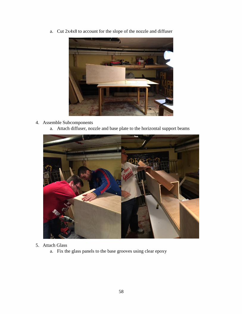
58

a. Cut 2x4x8 to account for the slope of the nozzle and diffuser

4. Assemble Subcomponents

a. Attach diffuser, nozzle and base plate to the horizontal support beams

5. Attach Glass

a. Fix the glass panels to the base grooves using clear epoxy

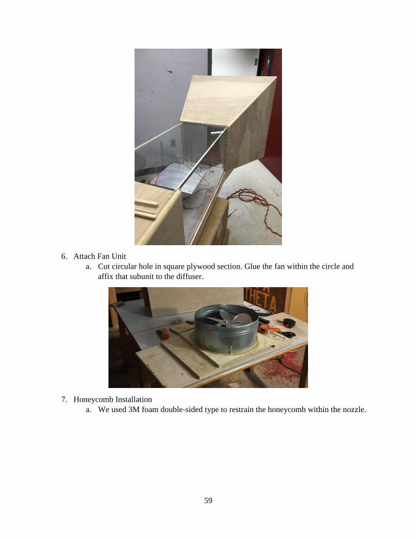
59

6. Attach Fan Unit

a. Cut circular hole in square plywood section. Glue the fan within the circle and

affix that subunit to the diffuser.

7. Honeycomb Installation

a. We used 3M foam double-sided type to restrain the honeycomb within the nozzle.

60

8. Screen Application

a. Apply a screen to the nozzle to prevent foreign object suction.

b. Apply metallic screen to the diffuser to prevent hand injury – a “requirement” of

Torbjorn Bergstrom, PhD Pursuant.

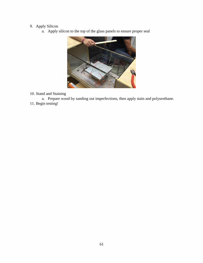
61

9. Apply Silicon

a. Apply silicon to the top of the glass panels to ensure proper seal

10. Stand and Staining

a. Prepare wood by sanding out imperfections, then apply stain and polyurethane.

11. Begin testing!

62

Appendix B: Instrumentation and Unit Setup

Infrared Laser Thermometer

Fan Unit Controller

Hot Wire Anemometer

Hot Wire Anemometer

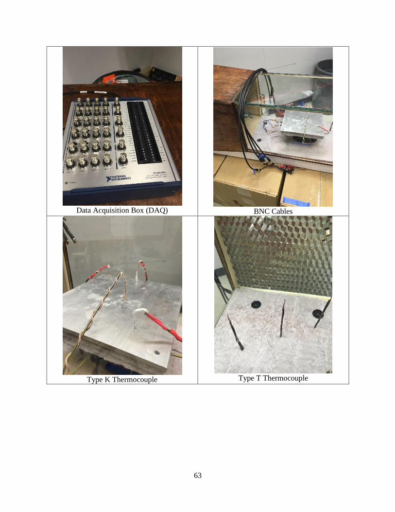
63

Data Acquisition Box (DAQ)

BNC Cables

Type K Thermocouple

Type T Thermocouple

64

Thermocouple Cold Junction

Cold Junction Demonstration

Variac

Suction Cup Handle

65

Fan

Fan Specifications

Honeycomb

Silicon

66

BNC Connections for setup

BNC Connections for setup

Complete Setup

67

Complete Demonstration Unit Set-up

1. Move Demonstration Unit to Classroom

2. Ensure you have the following equipment (Photos Above)

a. DAQ BOX

b. BNC Cables attached to correct Thermocouples (Labeled 0-6)

c. Laptop Computer with LabVIEW and Specific Program

d. Cups

e. ICE

f. Extension Cords for Fan, Variac, DAQ Box, and Laptop

g. Hot Wire Anemometer

h. Fan Speed Controller

3. Fill cups with ice and water

4. Place three thermocouple cold junctions into cups of ice-water

5. Connect BNC Cables to DAQ Box

a. Connect across the top most row Thermocouples 0,1,2,3

b. Connect across the second row from top Thermocouples 4,5,6

6. Connect DAQ Box to power source and ensure power switch is on

7. Connect DAQ Box to Computer

8. Open LabVIEW Program on Computer

9. Connect RED Banana Plug from Power cord to RED Input Slot on Variac

10. Connect BLACK Banana Plug from Power cord to BLACK Input Slot on Variac

11. Connect RED Banana Plug from Demonstration Device to RED Output Slot on Variac

12. Connect BLACK Banana Plug from Demo Device to BLACK Output Slot on Variac

13. Ensure Variac power switch is off and voltage set to ZERO

14. Connect Power Cord to outlet

15. Ensure Fan Speed Controller is in off position

16. Connect Fan Speed Controller to fan and then to extension cord and then to outlet

17. Connect Hot Wire Anemometer (HWA) to Phone

18. Place HWA inside test section

19. Begin running the LabVIEW program by pushing the white arrow in top left

a. Do not hit button that says run program continuously

20. Please refer to Section 3.3 for step-by-step directions for running experiments

21. Set Variac to desired voltage and turn on power switch

22. Have Fun and Be Safe!

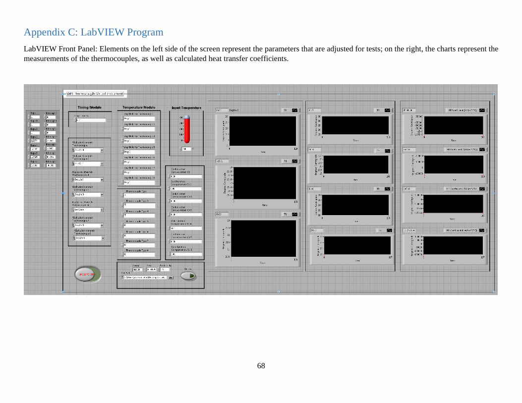
68

Appendix C: LabVIEW Program

LabVIEW Front Panel: Elements on the left side of the screen represent the parameters that are adjusted for tests; on the right, the charts represent the

measurements of the thermocouples, as well as calculated heat transfer coefficients.

69

LabVIEW Block Diagram 1: This represents the processing parts of the LabVIEW program. They are all inside a while loop that continuously runs

thermocouple measurements and calculates the heat transfer coefficient.

70

LabVIEW Block Diagram 2: This represents the part that is outside the while loop. This function

writes labels the columns of an excel file.

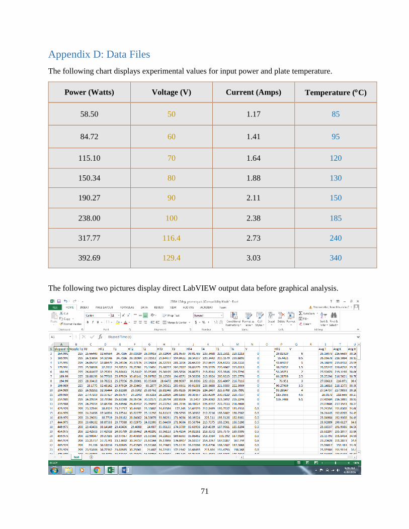
71

Appendix D: Data Files

The following chart displays experimental values for input power and plate temperature.

Power (Watts) Voltage (V) Current (Amps) Temperature (C)

58.50 50 1.17 85

84.72 60 1.41 95

115.10 70 1.64 120

150.34 80 1.88 130

190.27 90 2.11 150

238.00 100 2.38 185

317.77 116.4 2.73 240

392.69 129.4 3.03 340

The following two pictures display direct LabVIEW output data before graphical analysis.

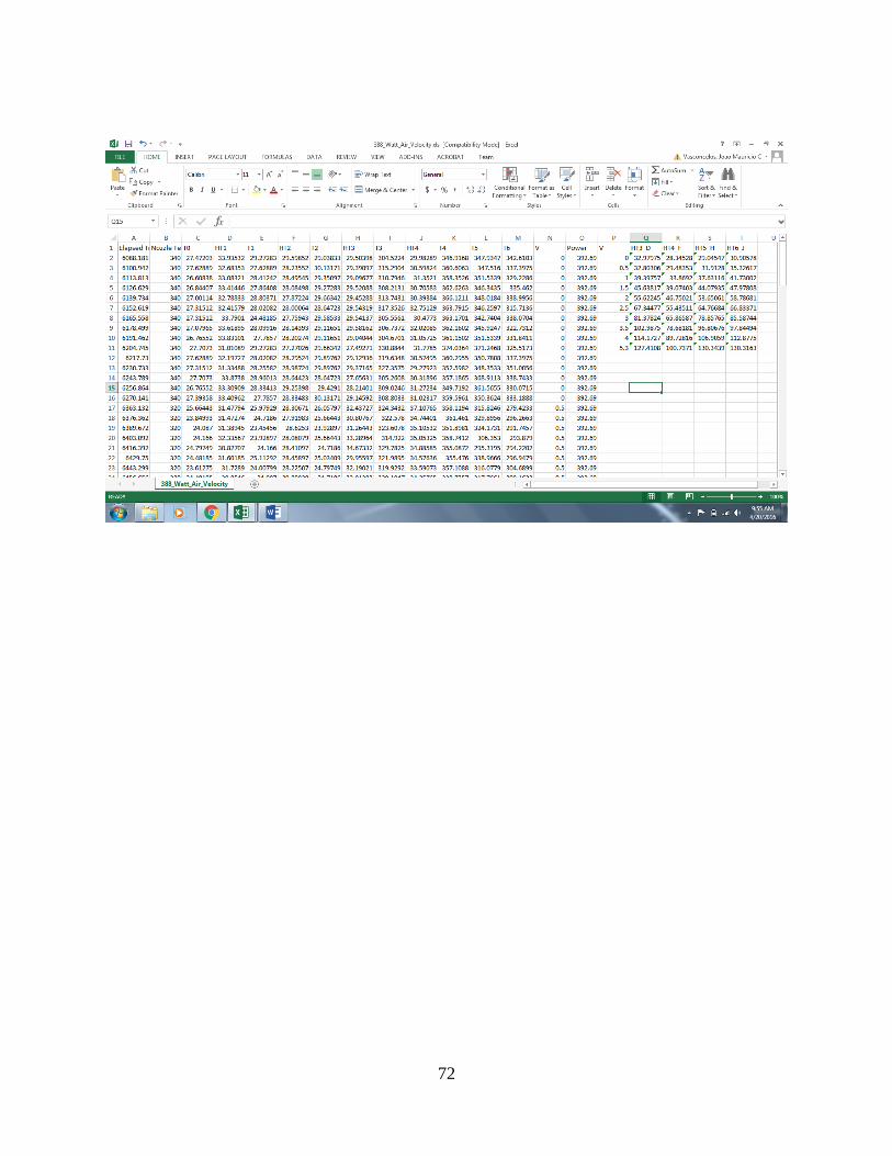
72

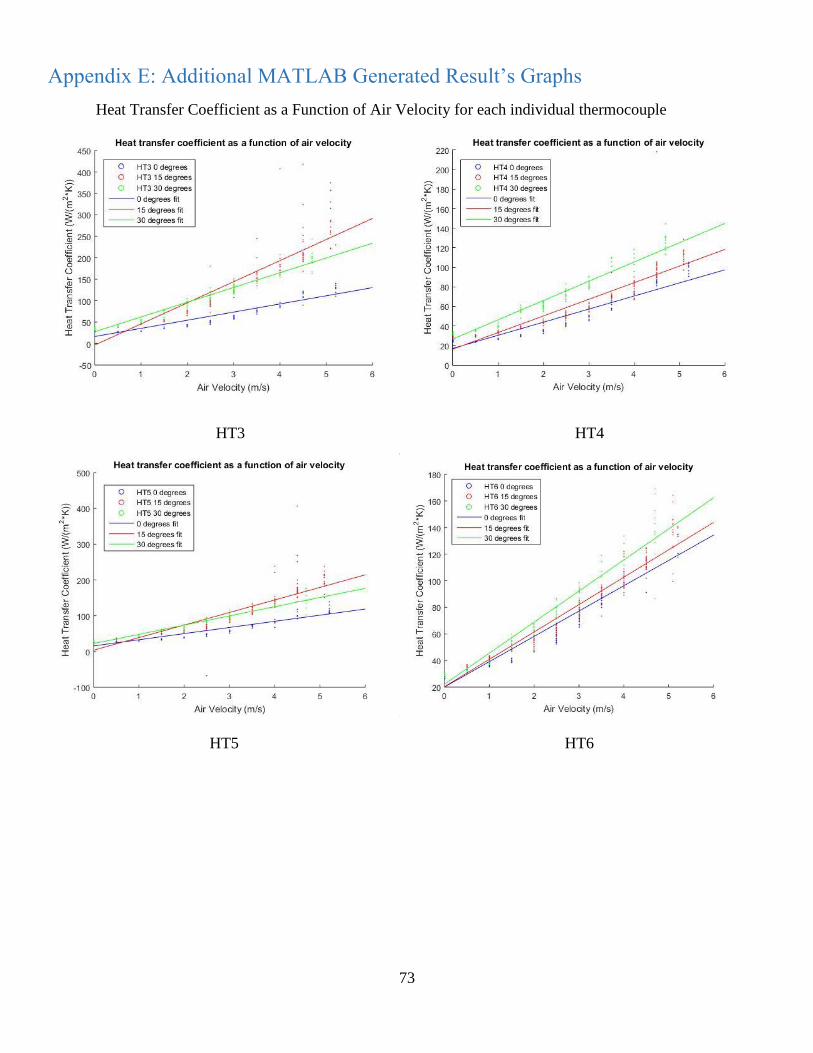
73

Appendix E: Additional MATLAB Generated Result’s Graphs

Heat Transfer Coefficient as a Function of Air Velocity for each individual thermocouple

HT5 HT6

HT3 HT4

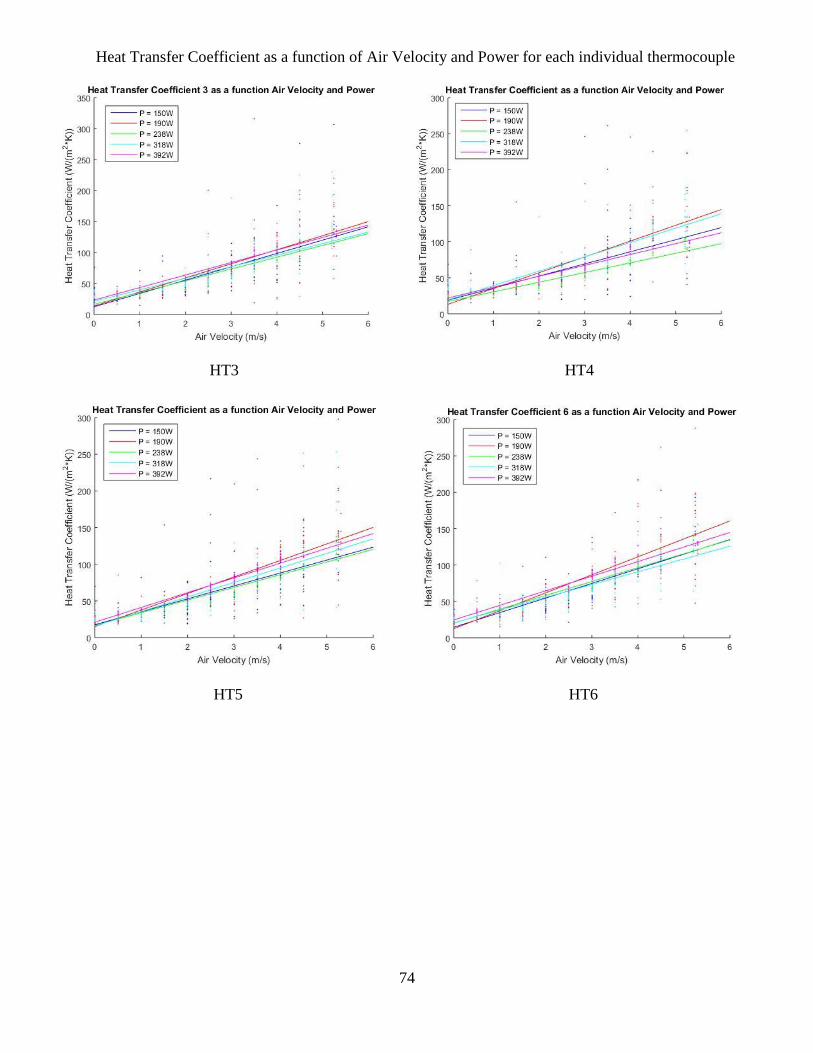
74

Heat Transfer Coefficient as a function of Air Velocity and Power for each individual thermocouple

HT3 HT4

HT5 HT6

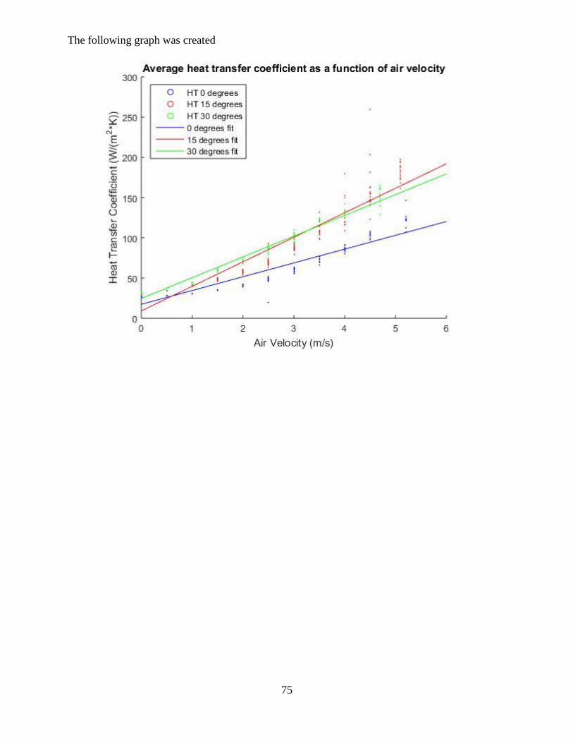
75

The following graph was created

76

Appendix F: ANSYS Generated Fluent Report

77

78

79

80

81

82

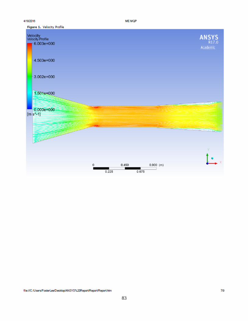
83

84

85

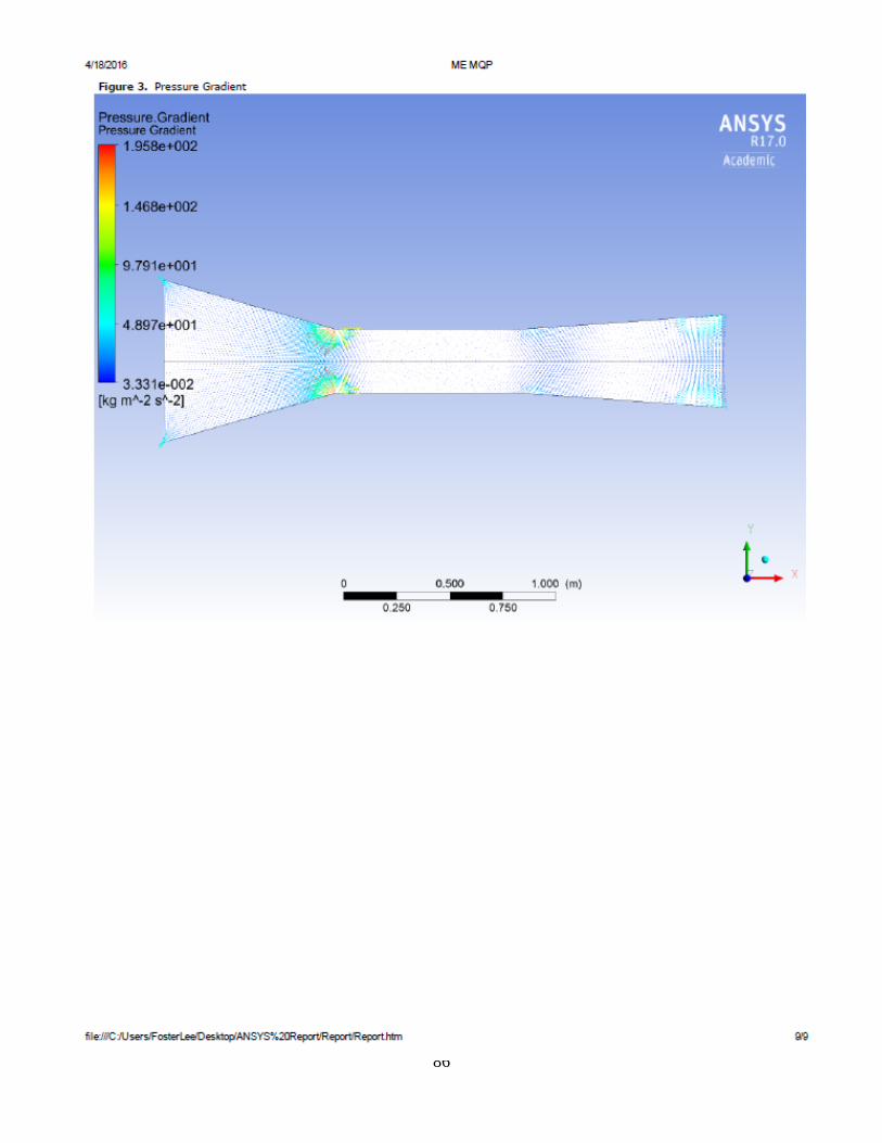
86

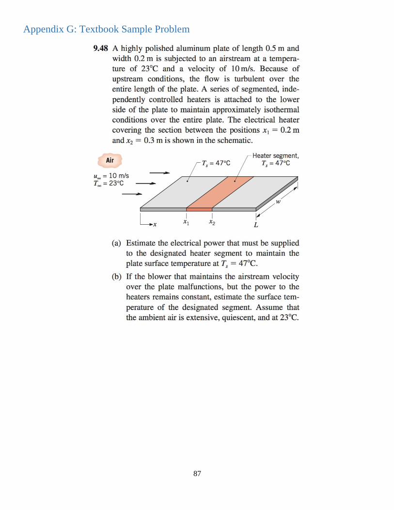
87

Appendix G: Textbook Sample Problem