heat transfer of oxy-fuel flames to glass
TRANSCRIPT

Heat transfer of oxy-fuel flames to glass
Citation for published version (APA):Remie, M. J. (2007). Heat transfer of oxy-fuel flames to glass. Technische Universiteit Eindhoven.https://doi.org/10.6100/IR617047
DOI:10.6100/IR617047
Document status and date:Published: 01/01/2007
Document Version:Publisher’s PDF, also known as Version of Record (includes final page, issue and volume numbers)
Please check the document version of this publication:
• A submitted manuscript is the version of the article upon submission and before peer-review. There can beimportant differences between the submitted version and the official published version of record. Peopleinterested in the research are advised to contact the author for the final version of the publication, or visit theDOI to the publisher's website.• The final author version and the galley proof are versions of the publication after peer review.• The final published version features the final layout of the paper including the volume, issue and pagenumbers.Link to publication
General rightsCopyright and moral rights for the publications made accessible in the public portal are retained by the authors and/or other copyright ownersand it is a condition of accessing publications that users recognise and abide by the legal requirements associated with these rights.
• Users may download and print one copy of any publication from the public portal for the purpose of private study or research. • You may not further distribute the material or use it for any profit-making activity or commercial gain • You may freely distribute the URL identifying the publication in the public portal.
If the publication is distributed under the terms of Article 25fa of the Dutch Copyright Act, indicated by the “Taverne” license above, pleasefollow below link for the End User Agreement:www.tue.nl/taverne
Take down policyIf you believe that this document breaches copyright please contact us at:[email protected] details and we will investigate your claim.
Download date: 27. Jan. 2022


Heat Transfer of Oxy-Fuel Flames to Glass
PROEFSCHRIFT
ter verkrijging van de graad van doctor aan de
Technische Universiteit Eindhoven, op gezag van deRector Magnificus, prof.dr.ir. C.J. van Duijn, voor een
commissie aangewezen door het College voor
Promoties in het openbaar te verdedigen
op woensdag 28 februari 2007 om 16.00 uur
door
Marinus Jan Remie
geboren te Breda

Dit proefschrift is goedgekeurd door de promotoren:
prof.dr. L.P.H. de Goeyen
prof.dr. L.E.M. Aldén
Copromotor:
dr. K.R.A.M. Schreel
Dit proefschrift is mede tot stand gekomen door financiële bijdrage van
Philips Lighting B.V.
Copyright c© 2007 by M.J. Remie
All rights reserved. No part of this publication may be reproduced, stored ina retrieval system, or transmitted, in any form, or by any means, electronic,
mechanical, photocopying, recording, or otherwise, without the prior permis-
sion of the author.
Cover design: Koen Schreel & Martin Remie
Cover: Prometheus, overlooking the heat-flux landscape (figure 3.10, page 48),gives oxy-fuel to mankind
Printed by the Eindhoven University Pres.
A catalogue record is available from the Library Eindhoven University of
Technology
ISBN-10: 90-386-2669-x
ISBN-13: 978-90-386-2669-7

Contents
1 General Introduction 1
1.1 Impinging flame jets . . . . . . . . . . . . . . . . . . . . . . . . 1
1.2 Background . . . . . . . . . . . . . . . . . . . . . . . . . . . . . 2
1.3 Heat transfer from impinging flame jets: state-of-the-art . . . . 3
1.3.1 Convection . . . . . . . . . . . . . . . . . . . . . . . . . 5
1.3.2 Thermochemical Heat Release . . . . . . . . . . . . . . 7
1.3.3 Radiation . . . . . . . . . . . . . . . . . . . . . . . . . . 9
1.4 Problem description . . . . . . . . . . . . . . . . . . . . . . . . 10
1.4.1 Industrial problems . . . . . . . . . . . . . . . . . . . . 10
1.4.2 Scientific problems . . . . . . . . . . . . . . . . . . . . 11
1.5 Objectives . . . . . . . . . . . . . . . . . . . . . . . . . . . . . . 12
1.6 Approach . . . . . . . . . . . . . . . . . . . . . . . . . . . . . . 13
1.7 Outline . . . . . . . . . . . . . . . . . . . . . . . . . . . . . . . 15
2 Flame Jet Properties of Bunsen-Type Flames 17
2.1 Introduction . . . . . . . . . . . . . . . . . . . . . . . . . . . . 17
2.2 Expansion of an unburnt gas plug flow over the flame front . . 18
2.3 Experimental validation . . . . . . . . . . . . . . . . . . . . . . 22
2.4 Discussion . . . . . . . . . . . . . . . . . . . . . . . . . . . . . 27
2.5 Conclusions . . . . . . . . . . . . . . . . . . . . . . . . . . . . 29
3 Heat transfer from a laminar flame jet to a flat plate 31
3.1 Introduction . . . . . . . . . . . . . . . . . . . . . . . . . . . . 31
3.2 Analytical solution for the heat transfer for small spacings . . . 32
3.3 Numerical validation . . . . . . . . . . . . . . . . . . . . . . . . 39
iii

iv Contents
3.4 Extension of the solution for the heat transfer to large spacings 44
3.5 Conclusions . . . . . . . . . . . . . . . . . . . . . . . . . . . . 49
4 Heat transport inside a glass product heated by a flame jet 51
4.1 Introduction . . . . . . . . . . . . . . . . . . . . . . . . . . . . 514.2 Heat-flux distribution . . . . . . . . . . . . . . . . . . . . . . . 52
4.3 Temperature distribution in the quartz plate . . . . . . . . . . . 58
4.4 One-dimensional solution for the temperature distribution . . . 60
4.5 Experimental validation . . . . . . . . . . . . . . . . . . . . . . 64
4.5.1 Single-point temperature measurements . . . . . . . . 654.5.2 Two-dimensional temperature measurements . . . . . . 70
4.6 Conclusions . . . . . . . . . . . . . . . . . . . . . . . . . . . . 75
5 Practical applications 775.1 Introduction . . . . . . . . . . . . . . . . . . . . . . . . . . . . 77
5.2 From burner nozzle to product: prediction of the heat flux . . . 78
5.3 Application to flame jets positioned inline . . . . . . . . . . . . 83
5.4 Pressure drop over the burner: a comparison . . . . . . . . . . 865.5 Critical blowoff gradient . . . . . . . . . . . . . . . . . . . . . . 88
5.6 Burner fouling . . . . . . . . . . . . . . . . . . . . . . . . . . . 90
6 Summarizing conclusions 93
Nomenclature 97
A Solution convective heat flux for two-dimensional case 101
References 109
Abstract 117
Samenvatting 119
Curriculum Vitae 121
Dankwoord 123

Chapter
1General Introduction
1.1 Impinging flame jets
The heat transfer of laminar impinging oxy-fuel flame jets will be analyzed in
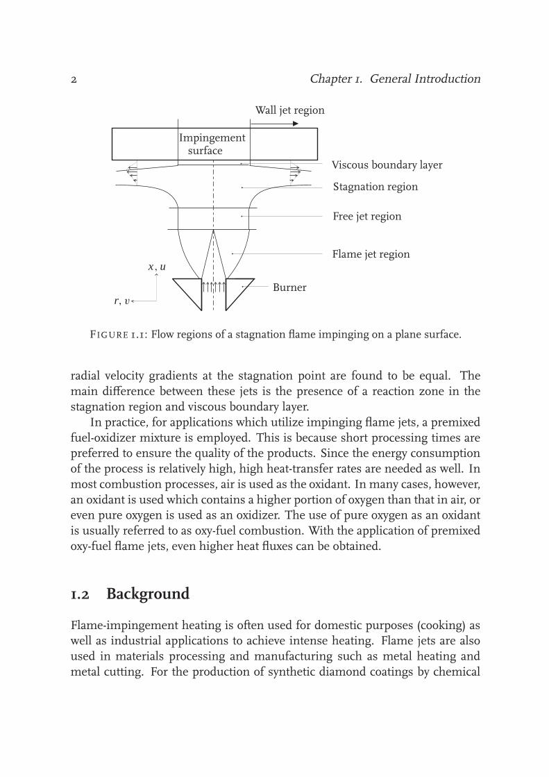
detail. A generalized picture of a single circular flame jet is shown schemati-cally in figure 1.1. Four characteristic regions can be distinguished in the flow
structure of an impinging axisymmetric flame jet on a flat plate: the flame jet
region, the free jet region, the stagnation flow region and the wall jet region.
When an unburnt gas mixture exits the burner nozzle, it enters the flame jetregion. Consequently, it experiences a sudden expansion as the gases react in
the flame front. The resulting burnt gas mixture now enters the free jet region,
where the velocity remains constant for the laminar case if the plate has no
perceptible influence on the flow. In the stagnation region the velocity of the
mixture decreases in the axial direction as a result of the influence of the plateon the flow. Near the plate a viscous boundary layer will develop which has
approximately a constant thickness in the impingement zone [41]. When the
jet turns in radial direction and the gases enter the wall jet region, the viscous
boundary layer thickness will increase. Since the different time scales in eachregion differ significantly, the regions can be decoupled, treated separately, and
coupled again afterwards. Using this approach, we will show how the heat-flux
distribution of an impinging laminar oxy-fuel flame jet to a glass product can
be determined.
Impinging flame jets are commonly approximated by hot inert jets, sincethe flow behavior of both types of jets is comparable. According to Viskanta
[66], the aerodynamics of a single flame jet is very similar to the aerodynamics
of a single isothermal jet. Experiments by Van der Meer [43] showed that the
1
2 Chapter 1. General Introduction
Wall jet region
Viscous boundary layer
Stagnation region
Free jet region
Flame jet region
Burner
Impingementsurface
x, u
r, v
FIGURE 1.1: Flow regions of a stagnation flame impinging on a plane surface.
radial velocity gradients at the stagnation point are found to be equal. The
main difference between these jets is the presence of a reaction zone in the
stagnation region and viscous boundary layer.
In practice, for applications which utilize impinging flame jets, a premixed
fuel-oxidizer mixture is employed. This is because short processing times arepreferred to ensure the quality of the products. Since the energy consumption
of the process is relatively high, high heat-transfer rates are needed as well. In
most combustion processes, air is used as the oxidant. In many cases, however,
an oxidant is used which contains a higher portion of oxygen than that in air, oreven pure oxygen is used as an oxidizer. The use of pure oxygen as an oxidant
is usually referred to as oxy-fuel combustion. With the application of premixed
oxy-fuel flame jets, even higher heat fluxes can be obtained.
1.2 Background
Flame-impingement heating is often used for domestic purposes (cooking) aswell as industrial applications to achieve intense heating. Flame jets are also
used in materials processing and manufacturing such as metal heating and
metal cutting. For the production of synthetic diamond coatings by chemical

1.3. Heat transfer from impinging flame jets: state-of-the-art 3
vapor deposition, premixed impinging flame jets have been used as well [13].
Impinging flames can also be found in the glass industry. Glass products aremelted, cut, formed, annealed, softened and shaped using flame jets in many
aspects of the glass fabrication processes.
In conventional industrial furnaces, the predominant heat-transfer mech-
anism is radiation, while convection accounts for a relatively smaller fraction[65]. In modern rapid heating furnaces, the flames impinge directly on the tar-
get. This way, the role of radiation is smaller and convection gains the upper
hand. Furthermore, higher heat fluxes are achieved. In the case that the target
is not placed inside a furnace enclosure, the role of radiation can be neglected.
The use of directly impinging flame jets with high velocity burners insteadof furnaces has a lot of advantages. First of all, the heat transfer is enlarged.
Furthermore, energy can be saved by switching on the burners only when heat
is demanded [43]. Also, to prevent the material from melting, the burners can
be turned off. Finally, the heat can be applied locally.
The advantage of being able to heat a product locally, can be a major dis-advantage as well. The heat-flux distribution is nonuniform, particularly on a
large target surface [65]. As a result, however, hot spots can be created at the
stagnation point and overheating at such spots can occur. For this reason, the
rapid heating technology of flame-impingement heating raises the need for theknowledge of the heat-flux distribution of a flame jet impinging on a product.
This way, the optimum firing strategy for a given material can be determined.
1.3 Heat transfer from impinging flame jets: state-of-the-
art
Originally, heat-transfer relations applicable for impinging flame jets were taken
from aerospace technology. Heat-transfer correlations concerning flame jet im-pingement show a lot of resemblances with aerospace applications [6]. High
temperatures at the stagnation point of aerospace vehicles are produced as
these vehicles travel through the atmosphere. Consequently, the atmospheric
gases will dissociate into many chemical species. Therefore, very high heat
fluxes arise in that region. Research on quantifying that heat flux have resultedin several semi-analytical solutions. In the aerospace applications, the vehicle
moves through the atmosphere where the gases are relatively stagnant. In the
case of impinging flame jets, the burnt gases move around a stationary target.
4 Chapter 1. General Introduction
Therefore, the relative motion is similar in both cases and the solutions found
for the heat transfer in aerospace situations are used for flame-impingementheating studies as well.
Flame jet impingement studies identify four heat-transfer mechanisms:
convection, radiation, thermochemical heat release (TCHR) and condensation
[5, 6, 64, 66]. The thermal and flow conditions determine the relative impor-tance of each mechanism. For example, forced convection will be the most
important mechanism in the absence of an enclosure. It the target is placed
inside a hot furnace, however, radiation from the furnace walls will predom-
inate over convection. Condensation can also contribute to the heat flux at a
cool target [25], but this process usually is only important when the target hasa temperature below 100◦C.
In the following subsections we will discuss the several heat-transfer mech-
anisms more extensively. Some correlations concerning the heat transfer will
be presented. Let us first consider some nondimensional numbers that are
commonly used in heat-transfer analysis.The Reynolds number (Re) determines the ratio of the inertial forces to the
viscous forces in a flow:
Re = ρUl
µ= Ul
ν, (1.1)
with ρ the fluid density [kg/m3], U the fluid velocity, l the characteristic lengthscale (usually the diameter of the jet), µ the dynamic viscosity [kg/(m·s)] and ν
the kinematic velocity [m2/s]. For laminar flows, the Reynolds number will below. The Reynolds number will be high for turbulent flows, while a transition
flow exists in between. Up to a Reynolds number of Re = 2500, an imping-
ing jet is considered to be laminar [51]. The ratio of momentum diffusivity to
thermal diffusivity is expressed by the Prandtl number (Pr):
Pr = ν
α, (1.2)
where α = λ/(ρ · cp) is the thermal diffusivity [m2/s], with λ the thermal con-ductivity [W/(m·K)] and cp the specific heat at constant pressure [J/(kg·K)]. Formany gases, the Prandtl number is typically equal to Pr = 0.7. The Nusselt
number (Nu) is defined as the ratio of the convective to the conductive heat-
transfer rates:
Nu = hl
λ, (1.3)
1.3. Heat transfer from impinging flame jets: state-of-the-art 5
with h the heat-transfer coefficient [W/(m2·K)]. The Nusselt number is typically
a function of Re and Pr for forced convection flows and is used to determinethe convective heat-transfer rate.
1.3.1 Convection
Convective heat transfer is dependent of several factors like the aerodynam-
ics of the jet, the turbulence intensity, the separation distance between burner
and target surface, the shape of the target, the fuel-oxidizer combination, the
stoichiometry, recombination of radicals at the target and whether the jet is apremixed or diffusion flame [66]. The effect of the equivalence ratio was stud-
ied by Hargrave et al. [25]. The results show that variations in equivalence
ratio away from approximately stoichiometric conditions lead to a shifting of
the flame reaction zone downstream and to a decrease in the maximum rate of
heat transfer from the flame. Experimental results [25, 63] show that the equiv-alence ratio also affects the local heat-flux distribution, since it effects the entire
combustion process. Rigby and Webb [57] found that the heat flux to a disk is
relatively constant for natural gas-air diffusion flames for larger nozzle-to-plate
spacings. Mizuno [45] experimentally found that the heat flux increases withdecreasing separation distance for premixed methane-air flames. This result
was explained by the fact that the smaller separation distance allowed less en-
trainment of cold ambient air into the flame, resulting in a higher burnt gas
temperature and thus a higher heat flux.
Forced convection is the dominant mechanism for flames with tempera-tures up to 1700 K [28]. Burner exit velocities typically are high enough, so
buoyancy effects can be neglected. For such a low temperature flame im-
pingement with no furnace enclosure, the share of forced convection may be
70 − 90% [11, 44]. Therefore, for these flames forced convection has generallybeen the only mechanism considered. The heat release from flame chemical
reactions at or near the target is not taken into account for this case and there-
fore this mechanism is sometimes referred to as frozen flow [6].
The heat transfer from impinging flows to objects with different geometries
have been studied extensively. Semi-analytical relations have been derived forthe heat transfer to the stagnation point. In these relations the so-called velocity
gradient comes into play. From potential flow theory, the axial velocity decrease
due to stagnation near the stagnation point and the radial velocity increase just

6 Chapter 1. General Introduction
outside the boundary layer for the axisymmetric case may be given by:
u = −2βx and v = βr, (1.4)
where the directions of x, u, r and v are shown in figure 1.1 and where β isdefined as the velocity gradient just outside the boundary layer [1/s]:
β =(
∂v
∂r
)
r=0
. (1.5)
The value of this velocity gradient depends on the shape and size of the body
of impingement and of the uniform flow velocity. The value for the velocitygradient of a circular disc immersed in a uniform flow is found from potential
flow solutions [30, 36]:
β = 4U
πd, (1.6)
with d diameter of the disc [m] and U the uniform flow velocity [m/s]. The
velocity gradient for this configuration has been determined experimentally aswell bymeasuring the radial pressure distribution on the impingement surface.
If viscous effects are negligible, Bernoulli’s theorem can be used to determine
β:
β =(
d
dr
√
2(pw − p(r))
ρ
)
r=0
, (1.7)
where the pressure at the stagnation point is given by pw [N/m2]. The value for
the velocity gradient was experimentally found to be equal to β = U/d [36, 34].
From experimental results it appeared that this value for the velocity gradientβ also applies for a uniform jet with diameter d impinging on a flat plate [43].
Sibulkin [61] derived a theoretical solution for the heat transfer near the for-
ward stagnation point of a body of revolution. He assumed the flow to be lam-
inar, incompressible and of low speed. His solution has been regarded as the
basis of all other theoretical and experimental results. Using the axisymmet-ric boundary layer equations, he found the following relation for the Nusselt
number at the stagnation point:
Nud = 0.763d
(
β
ν∞
)0.5
Pr0.4∞ , (1.8)

1.3. Heat transfer from impinging flame jets: state-of-the-art 7
where the Nusselt number is based on the diameter of the body of revolution
d. The subscript ∞ signifies the value of the corresponding parameter in theuniform flow. Furthermore, the constant 0.763 was determined numerically.
The rate of heat transfer can now be expressed as follows:
q = Nudλ(Tw − T∞)
d= 0.763 (βρ∞µ∞)0.5 Pr−0.6
∞ cp,∞(T∞ − Tw), (1.9)
with q the heat flux [W/m2] and Tw the temperature at the stagnation point ofthe body of revolution [K].
Turbulence can enhance the heat transfer. Horsley et al. [26] found that
the stagnation point heat transfer for impinging natural gas-air flames can be
a factor of 1.2 − 1.8 higher than predicted for laminar flows by Sibulkin [61].Van der Meer [43] showed that the heat transfer is only enhanced if the target
surface is placed outside of the potential core of the free jet. He used linear
regression to correlate the experimental heat-flux data as:
q = (1 + γ )0.763 (βρ∞µ∞)0.5 Pr−0.6∞ (hS
∞ − hSw), (1.10)
where γ is a turbulence-enhancement factor and hS =∫
cpdT the sensible
enthalpy [J/kg].
1.3.2 Thermochemical Heat Release
Flame jets can be operated with an increase of the amount of oxygen in theoxidizer stream, which leads to a higher burning velocity of the flame. There-
fore, the flame jet can be operated with higher gas velocities. Furthermore,
the removal of nitrogen in the burnt gases, which acts as a heat sink, causes
a much higher flame temperature. For instance, stoichiometric methane-airflames have a temperature of about 2200 K, while stoichiometric methane-
oxygen flames reach temperatures of about 3000 K. The higher unburnt gas
velocity as well as the increased flame temperature cause the effect that higher
heat-transfer rates are obtained.
The products of many combustion processes contain dissociated species.The degree of dissociation increases as the flame temperature increases. Since
oxygen enriched flames reach high temperatures, their products contain a lot
of free radicals due to dissociation. As the gases cool down due to impingement

8 Chapter 1. General Introduction
near the cold surface, they exothermically recombine to more stable products.
The radical recombination causes an additional heat release. This mechanismis called Thermochemical Heat Release (TCHR). TCHR can be of the same
order of magnitude as forced convection at high temperatures.
Two chemical mechanisms are identified which initiate Thermochemical
Heat Release, namely equilibrium TCHR and catalytic TCHR [24]. If the chem-ical reaction time scale is smaller than the diffusion time scale, equilibrium
TCHR comes into play. The chemical reactions take place in the boundary
layer. In the case of catalytic TCHR, that is if the radicals have insufficient time
to react before they reach the surface, recombination may take place at the sur-
face. Nawaz [46] showed that a combination of equilibrium TCHR and catalyticTCHR can occur as well. In this case, the chemical reaction time scale is of the
same order of magnitude as the diffusion time scale. Some of the dissociated
species react in the boundary layer, others react catalytically at the surface.
Thermochemical Heat Release has commonly been combined with forced
convection into one heat-transfer correlation [21, 58, 15, 33]. The main reason isthat it is difficult to experimentally separate these mechanisms. Connoly and
Davis [15] expressed the stagnation point heat flux from amixture of dissociated
gases as:
q = 0.763 (βρ∞µ∞)0.5 Pr−0.6eq 1hT, (1.11)
where the total enthalpy difference 1hT driving the convective heat transfer
is equal to the sum of the sensible enthalpy difference 1hS and the chemicalenthalpy difference 1hC. The Prandtl number at equilibrium conditions is
given by:
Preq = Pr
[
1 + (Le − 1)
(
1hC
1hT
)]−1
, (1.12)
where the Lewis number defines the ratio of the heat diffusion to the speciesdiffusion. The Lewis number is defined as Le = λ/(ρcp D), with D the species
diffusivity coefficient [m2/s]. Stutzenberger [63] performed measurements of
the heat transfer from pure gas-oxygen impinging on metal surfaces. The re-
sults of the measured stagnation point heat fluxes for C2H2-O2, H2-O2, C3H8-
O2 and CH4-O2 flames showed good agreement with the relation derived byConnoly and Davis, equation (1.11). Recently Cremers [17] showed that the heat
flux including the heat release from the recombination of radicals can be cal-
culated by multiplying the convectional heat flux by a so-called TCHR factor,

1.3. Heat transfer from impinging flame jets: state-of-the-art 9
which is a function of the type of fuel, temperature of the surface and the
boundary velocity gradient.
1.3.3 Radiation
The influence of radiation on the heating process is highly dependent on wheth-er the target is isolated or placed in an enclosure. Two components contribute
to the thermal radiation heat transfer at the target surface, if the target is iso-
lated: nonluminous radiation and luminous radiation. In the presence of a
confinement such as a furnace, surface radiation will contribute a significant
part of the total heat flux. Comprehensive studies about thermal radiation heattransfer are lacking, however, since it is regarded as unimportant, compared
to convection. Other reasons are that a lot of computational and experimental
difficulties arise when taking radiation into account. Correlations which have
been developed predicting the radiative heat transfer are empirical and have no
theoretical basis. They are appropriate only for the particular systems studied.Nonluminous radiation is produced by gaseous combustion products such
as carbon dioxide and water vapor. The amount of radiation produced by the
gases depends on the gas temperature, partial pressures of the emitting species,
concentration of each emitting species and the optical path length through thegas. Although some studies indicate that nonluminous radiation amounts to a
significant part of the total heat flux to the target [27, 57], most studies consider
radiative heat transfer in nonluminous flames negligible [52, 66, 5, 28, 35]. Van
der Meer [43] stated that nonluminous radiation is negligible because of the
very low emissivity of a hot gas layer of small thickness.If a flame produces a lot of soot, luminous radiation can be a significant
component of the radiation heat transfer. The soot particles will radiate approx-
imately as a black body. This mechanism is especially important when solid
and liquid fuels are used. It is not commonly significant if gaseous fuels arecombusted, except when the flames are very fuel rich or if diffusion flames are
applied, which have a tendency to produce soot.
Surface radiation contributes significantly to the total heat transfer if the
target is heated inside an oven or furnace. Beer and Chigier [11] examined the
radiation contribution to the total heat transfer for a stoichiometric air-cokeoven gas flames impinging on the hearth of a furnace. The measured radiation
was at least 10% of the total heat flux. Ivernel and Vernotte [27] calculated
that radiation from furnace walls accounted for up to 42% of the total heat
10 Chapter 1. General Introduction
flux. From these results it is clear that radiation from the surrounding surfaces
becomes very important in high-temperature furnaces.
1.4 Problem description
1.4.1 Industrial problems
In the glass industry, many types of lamps are produced with all kinds of shapes
and sizes. The applications are manifold: from large lamps used for stadium
lighting to very small halogen lamps which can be found in headlights of cars.
For these small lamps, the distance between the tungsten wires and the en-
veloping lamp glass is very small. Since the tungsten wires reach temperaturesof up to 3000 K, quartz glass is chosen as the solid material. This is because
quartz glass has a much higher melting temperature compared to other glass
types.
The quartz glass needs, amongst other processes, to be melted, cut andformed during the lamp-making process, using impinging flame jets. Since
the quartz glass has a very high melting temperature, very high heat-transfer
rates from these flame jets to the target are needed. These high heat-transfer
rates are in most cases obtained by supplying the burners with a premixed
fuel-oxygen mixture. The heat transfer from the impinging flame jet will beincreased if the burner is operated with an oxy-fuel mixture, as explained in the
previous section. In other cases non-premixed or partially premixed burners
are used. These different types of burners are tuned by hand based on the prac-
tical experience of glass technicians to optimize the efficiency of the productionprocess.
This operating procedure brings along some drawbacks. The type of fuel
gas, the diameter of the burner, the distance between the burner nozzle and the
target, and the gas velocity are all chosen on a subjective basis. Therefore, long
cycle times are the result if new lamp making processes are developed. Thechange-over times are long as well, if the production line is adapted for another
product. Furthermore, it is not known whether the chosen set-up is optimal
and further optimization can not be verified.
1.4. Problem description 11
Flame front
Burner
Impingement
surface
H
URj
Rb
x, u
r, v
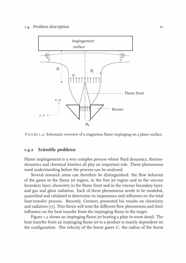
FIGURE 1.2: Schematic overview of a stagnation flame impinging on a plane surface.
1.4.2 Scientific problems
Flame impingement is a very complex process where fluid dynamics, thermo-
dynamics and chemical kinetics all play an important role. These phenomenaneed understanding before the process can be analyzed.
Several research areas can therefore be distinguished: the flow behavior
of the gases in the flame jet region, in the free jet region and in the viscous
boundary layer, chemistry in the flame front and in the viscous boundary layer,and gas and glass radiation. Each of these phenomena needs to be modeled,
quantified and validated to determine its importance and influence on the total
heat-transfer process. Recently, Cremers presented his results on chemistry
and radiation [17]. This thesis will treat the different flow phenomena and their
influence on the heat transfer from the impinging flame to the target.Figure 1.2 shows an impinging flame jet heating a plate in more detail. The
heat transfer from an impinging flame jet to a product is mainly dependent on
the configuration. The velocity of the burnt gases U , the radius of the burnt

12 Chapter 1. General Introduction
gas flow jet Rj and the distance from the flame tip to the plate H are important
parameters when the heat transfer needs to be calculated. No simple analyticalequations have been known yet, however, which relate the burner radius Rb
and the unburnt gas parameters such as the unburnt gas velocity on one hand
to the resulting burnt gas velocity U and burnt gas jet radius Rj on the other.
Semi-analytical relations to predict the convective heat transfer have beenstudied in the past, see section 1.3.1. These relations, however, are only appli-
cable for relatively large distances between the burner nozzle and the product.
On the other hand, from practical experience it turns out that the heat transfer
from the impinging flame to the target increases if the target is placed closer to
the flame jet. For this configuration, which is thus interesting from a practicalpoint of view, no relations are known. Furthermore, unrealistic results for the
heat transfer are obtained with existing relations for flows with low viscosity.
The effect of Thermochemical Heat Release was included in the existing
semi-analytical relations, such as in equation (1.11), by taking enthalpy differ-
ences into account. Flame calculations were usually not performed. If complexchemistry was taken into account, only mixtures of fuel and air were used. Cre-
mers [17] performed full chemical calculations for different fuels to determine
the influence of TCHR on the heat transfer of oxy-fuel stagnation flames to an
object. He found that the total heat transfer can be calculated, if the convectiveheat transfer is multiplied by a so-called TCHR-factor, to account for the contri-
bution of TCHR. This TCHR-factor is mainly a function of the choice of fuel,
plate temperature and the strain rate of the burnt gases.
1.5 Objectives
A research project has started in the year 2002 which is carried out as a cooper-
ation between Philips Lighting B.V. and Eindhoven University of Technology.
The main objective of the research is formulated as follows:
To gain scientific knowledge of oxy-fuel combustion in order to op-
timize the heat transfer to quartz and glass products and to transferthis knowledge to a practical application.
This objective can be divided in a part which is primarily of interest from a
scientific point of view (Eindhoven University of Technology) and a part which
is primarily of interest from a practical point of view (Philips). The research has

1.6. Approach 13
mainly been conducted within two Ph.D. projects. Cremers treated in his Ph.D.
project the problems which arise concerning radiation and chemistry. From thescientific point of view, the main objectives of the part of the research presented
in this thesis lead to the following questions which need to be answered:
How are the velocity and the jet width of the burnt gases after ex-
pansion over the flame front related to the unburnt gas velocity and
burner radius?
Can existing relations for the heat transfer of impinging flame jets,
which are applicable to situations where the target is placed rela-
tively far from the flame, be extended or reformulated so that they
are applicable for small distances between the flame and target as
well?
This research will lead to the development of burner design rules, which
can be used to relate fuel, burner and configuration properties to the heat flux.
As a result these relations can be used to reduce the process development cycle
time and the number of burner types. Furthermore, the controllability andefficiency of the lamp making production process will be increased.
1.6 Approach
As we have seen, the use of premixed impinging flame jets in the several stages
of the production of glass products often involves the use of pure oxygen in the
oxidizer stream. As a result, the temperature of the burnt gases is approxi-mately 3000 K, while the velocity of the burnt gases are of the order of mag-
nitude of 50 − 80 m/s. Since the flame jet usually is placed close to the glass
product to increase the heat transfer (typically a few millimeters between the
flame tip and the target), we will neglect buoyancy effects. The neglect of buoy-
ancy effects is often supported by the Richardson number. The Richardsonnumber Ri gives the ratio of natural convection to forced convection:
Ri = gα1T l
U 2, (1.13)
with g the gravitational acceleration [m/s2], l the typical length scale and α =−1/ρ(∂ρ/∂T )p the thermal expansion coefficient [1/K]. Since the value of the

14 Chapter 1. General Introduction
Richardson number Ri is of the order of 10−5 in our case, buoyancy effects can
be neglected.Because of the high temperature, the burnt gas flow is highly viscous: the
dynamic viscosity µ is typically of the order of magnitude of 10−4 kg/(m·s).Therefore the Reynolds number based on the burnt gas jet width is of the order
102 and the flow after the expansion over the flame front can be treated aslaminar. Since the burnt gas flow is laminar and the glass product is put close
to the flame tip, mixing with the ambient air causing a temperature decrease is
suppressed.
Cremers [17] has shown that the typical time scales which apply to the char-
acteristic regions of the flow structure (see figure 1.1) are different. The timescale of the flame chemistry is of the order of 10−5 s, while the time scale of
the viscous boundary layer of the stagnation flow is of the order of 10−4 s. The
time scale of the heating of the plate is dependent on the plate thickness. Since
the typical plate thickness is of the order of millimeters, the time scale is of
the order of 1 − 10 s. Because of these different time scales, the characteris-tic regions can be decoupled. After treating each zone separately, they can be
coupled again afterwards.
The distance between the flame tip and the plate H is chosen as an inde-
pendent input parameter for the determination of the heat flux to the target,see figure 1.2. This is not custom for the heat-flux relations found in litera-
ture. In literature, the distance from the burner nozzle exit to the target is
used as an input parameter. The usage of different fuels, however, results in
different flame heights because of the different burning velocities. Therefore,
different distances from the flame tip to the plate will be obtained. Especiallyfor close spacings, this has significant consequences. The viscous boundary
layer thicknesses will be different and therefore the different situations are not
comparable anymore. This is the reason we have chosen the distance from the
flame tip to the target as an independent parameter.Since we will focus on round jets, the problem is a two-dimensional ax-
isymmetric one. The use of a premixed oxy-fuel gas mixture results in a profile
of the burnt gases after expansion in the flame front, which can be approxi-
mated by a plug flow. At the edge of the stream tube, the velocity rapidly drops.
Therefore, the system can be reduced to a steady one-dimensional problem.We have shown earlier in section 1.3.1 that variations of equivalence ratio
away from approximately stoichiometric conditions lead to a decrease of the
heat transfer from the flame to the target. Therefore, we will focus on stoichio-

1.7. Outline 15
metric oxy-fuel mixtures.
Finally, the glass product is approximated by a plate, as shown in figures1.1 and 1.2. This is plausible, because the typical radius of the lamp tubes (or-
der 10−2 m) is usually larger than the shell thickness (order 10−4 − 10−3 m).
Furthermore, the width of the burnt gas jet is of the order of a few millime-
ters. Therefore, the temperature profile in the plate will be approximately one-dimensional.
1.7 Outline
In chapter 2 an analysis will be given about the expansion of unburnt gases over
the flame front. Using the global conservation equations of mass, momentum
and energy, a relation will be presented which relates the burner radius and theunburnt gas velocity on one hand to the burnt gas jet radius and the burnt gas
velocity on the other. These parameters are important since they serve as input
parameters for the calculation of the heat transfer from impinging flame jets to
glass products. Experimental validation using Particle Image Velocimetry willbe presented as well.
Existing semi-analytical relations predicting the convective heat transfer
from impinging flame jets the hot spot of a target are only applicable for rela-
tive large distances between the flame tip and the target. A new analytical rela-
tion for the convective heat transfer will be presented in chapter 3. Not only isthis relation applicable for relative large flame tip-to-plate distances, heat fluxes
from impinging flames situated closer to the target can be calculated as well.
Chapter 4 deals with the extension of the heat-flux relation so not only the
heat flux to the hot spot of the target can be calculated, but also the heat flux
for larger radial distances from the hot spot. Using the heat-flux relations, thetemperature distribution and therefore the thermal stresses in the product can
be calculated without solving the flow field of the burnt gas jet. Temperature
measurements based on phosphor thermometry will be presented with which
the heat-flux relations will be validated.Using the gathered knowledge on the heat transfer of impinging flame
jets, chapter 5 compares the heating of glass products using hydrogen-oxygen
flames on one hand and using methane-oxygen flames on the other. Some
problems encountered in practice will be treated as well. Finally, summarizing
conclusions will be given in chapter 6.

16 Chapter 1. General Introduction

Chapter
2Flame Jet Properties ofBunsen-Type Flames
2.1 Introduction
From practical experience it is known that in order to optimize the heat transferfrom an impinging flame jet to a target, the object to be heated should be placed
above the burner in such a way, that the flame front is not distorted, see figure
1.2. If a plate is positioned far enough above the burner accordingly, the flame
region and burnt gas region can be decoupled, treated separately and coupledafterwards again [16]. In this case the resulting burnt gas velocity and width of
the jet in the burnt gas region after expansion of the gases over the flame front
are very important parameters if the heat flux from the flame jet to the glass
product has to be determined.
For a flat flame, the resulting burnt gas velocity is equal to the unburnt gasvelocity multiplied by the expansion factor of the gas. This is not the case for
Bunsen-type flames. The resulting velocity of the burnt gases after the flame
front would be equal to the unburnt gas velocity for a Bunsen-type flame in the
other extreme case, if the flow tube of burnt gases could expand maximally. Itis generally known that for fuel-air flames the burnt gases experience a velocity
jump and therefore the expansion of the gases is not enough to keep the velocity
constant. For practical purposes, it is interesting to know what the relation is
between the expansion of the flow tube and the velocity of the burnt gases
on one hand and the expansion factor, the burning velocity, the burner radiusand unburnt gas velocity on the other. However, a simple expression or theory
to calculate the resulting velocity and jet width after expansion over the flame
front is lacking, although these are important parameters to determine the heat
17

18 Chapter 2. Flame Jet Properties of Bunsen-Type Flames
transfer of impinging jets.
Although a lot of work is done concerning the heat transfer of flame jets toproducts, the properties of the flame jet itself have been underexposed. Lewis
and Von Elbe treated the structure of laminar premixed flames [40], while Pe-
ters treated the movement of the flame front using expressions with the burn-
ing velocity [49]. These studies, however, are focussed on the structure of theflame front itself. The characteristics of the burnt gas flow after expansion of
the unburnt gases over the flame front are underexposed, whereas these are
very important parameters when the heat transfer to objects is considered.
This chapter shows how a simple relation between the known burner radius
and velocity in the unburnt mixture of Bunsen-type flames on one hand andthe jet radius and velocity in the resulting flame jet on the other can be derived.
The results of this relation make it possible to characterize the heat transfer in
a simple manner, when the flame is impinging on a flat product. This work,
however, has to be considered as a first initiative in this direction, since only
simple flow configurations are considered and since important phenomenalike flame stretch and flame curvature have not been taken into account yet.
Nonetheless, conservation of mass, momentum and energy is used to derive
the relation. The next section shows how the relation has been derived using
the conservation equations. Particle Image Velocimetry experiments have beenperformed to validate the theoretical results. Section 2.3 describes how these
experiments were performed and shows a comparison with the model. The
deviations are discussed in the subsequent section, followed by conclusions in
the last section.
2.2 Expansion of an unburnt gas plug flow over the flame
front
A schematic view of the cylindrical Bunsen flame considered is shown in figure
2.1. We will use this figure to derive the equations with which the velocity u2,
pressure p2 and jet radius Rj of the burnt gases can be calculated. Therefore it
is assumed that the velocity (u1) of the unburnt gases, the burner radius (Rb),
the burning velocity (sL) and the temperatures in the unburnt (Tu) and burnt(Tb) gases are known. The model, however, is subject to some restrictions.
The velocity profile at the burner exit is taken to be flat. Furthermore, the
burning velocity sL is constant over the entire flame front. As a result, the flame

2.2. Expansion of an unburnt gas plug flow over the flame front 19
Symmetry axis
Flame front
Stream line
Unburnt
Burnt
Burnt
Rj
Rb
u1
u1
u2
p1
p2
u3
u1//
u1//
τ × sL
sL
FIGURE 2.1: Schematic of the gas velocity increase over the flame front.
front forms a straight cone with a sharp tip and the velocities directly after theflame front are uniform as well. It is further assumed that the burnt gas flow
develops in a plug flow after the flame tip. Therefore, this indicates that the
associated pressures will be uniform as well in the model. The flow behavior at
the flame tip and at the burner edge where the flame stabilizes on the nozzleis significantly different. In reality this influence, however, is assumed to be
small. Furthermore, shear effects between the jet and the surroundings are
neglected and the burnt gas flow is assumed to be isentropic.
Zooming into the flame front, it is shown that the gases experience a ve-
locity jump normal to the flame front. Peters [49] has shown that for the thinflame approximation this velocity jump equals
n · (u1 − u3) = (τ − 1)sL, (2.1)
with τ = ρu/ρb, ρu being the density of the unburnt mixture [kg/m3], ρb the
density of the burnt mixture, u1 the gas velocity vector before the flame front
[m/s], u3 the gas velocity vector after the flame front and n the unity vector

20 Chapter 2. Flame Jet Properties of Bunsen-Type Flames
normal to the front and directed to the unburnt gases. The equations for con-
servation of mass and momentum over the flame front become
ρu(n · u1) = ρb(n · u3), (2.2)
p1 + ρu(n · u1)2 = p3 + ρb(n · u3)
2. (2.3)
We define a control volume in figure 2.1, which is formed by the outlet of
the burner nozzle (denoted by the number ’1’ in the figure), the symmetry axis,
the plug flow of burnt gases with radius Rj formed above the burner (’2’ in thefigure), and the two dashed lines. Since there is no pressure drop over either
boundary of the control volume but only over the flame front, the pressure at
the outlet of the burner nozzle equals p1 and the pressure at the top side of
the control volume equals p2, which is assumed to be equal to the ambientpressure. The equations for conservation of mass and momentum for this
control volume become:
ρuπ R2bu1 = ρbπ R2
j u2, (2.4)
(p1 + ρuu21)π R2
b + p2π(R2j − R2
b) = (p2 + ρbu22)π R2
j , (2.5)
where the buoyancy term in the momentum equation is assumed to be small
and therefore negligible. This can be shown as follows. If the buoyancy termin the momentum equation is integrated over the control volume, it can be ap-
proximated by ρugπ R2j H , where H is the height of the control volume. Com-
pared to the term ρuu21π R2
b , it can be seen that the effect of acceleration of the
burnt gases as a result of gravity is not considerable as long as H < u21 R2
b/(gR2j ).
This means that for a methane-air flame, with a typical unburnt gas velocity of
1 m/s, H < u21/g ≃ 10−1 m. The effect for methane-oxygen flames will even be
less, where the typical unburnt gas velocity is 102 m/s, so H < u21/g ≃ 103 m.
With this assumption, the equation for conservation of mechanical energy after
the flame front becomes:
p3 + 1
2ρbu2
3 = p2 + 1
2ρbu2
2. (2.6)
Since we assume that the unburnt gas velocity u1 at the exit of the burnernozzle, the expansion term τ and burning velocity sL are known, the pressure
p2, velocity u2 and jet radius of the burnt gases Rj can be calculated. Using
equation (2.2) and equation (2.3) results in a relation for the pressure jump

2.2. Expansion of an unburnt gas plug flow over the flame front 21
over the flame front. Combining conservation of mass, equation (2.4), and
momentum, equation (2.5), results in a relation between the pressure at theburner nozzle p1 and the pressure of the plug flow of burnt gases p2. The
relation between the pressure after the flame front p3 and the pressure in the
burnt gases p2 can be found by implementing u23 = u2
1 + (τ 2 − 1)s2L (see figure
2.1) in the equation for conservation of energy, equation (2.6):
p1 − p3 = ρus2L(τ − 1), (2.7)
p1 − p2 = ρuu1(u2 − u1), (2.8)
p3 − p2 = ρu
2τ
(
τ 2u21
R4b
R4j
− u21 − (τ 2 − 1)s2
L
)
, (2.9)
where the only unknowns are the pressures p2 and p3 and the width of theresulting plug flow of unburnt gases Rj.
The equation for the width of the resulting plug flow of unburnt gases Rj
as a function of the known parameters can now be found by combining the
pressure relations equations (2.7) - (2.9). The resulting polynomial has the
following form:
(
R2b
R2j
)2
− 2R2b
R2j
+ 2τ − 1
τ 2+(
sLu1
)2τ 2 − 2τ + 1
τ 2= 0, (2.10)
with solution x = 1 ± (1 − C)1/2, where x = R2b/R2
j and C = (2τ − 1)/τ 2 +(sL/u1)
2(τ 2−2τ+1)/τ 2. The solution with the plus sign describes a solution foran idealized V-flame, in which the radius of the flow of burnt gases is smaller
than the radius of the burner, Rj < Rb. This solution will not be treated here,
instead we will focus on the solution with the minus sign.
From equation (2.10), the solution of R2b/R2
j is a function of the indepen-dent dimensionless parameters τ and sL/u1. We now consider the solution for
certain limiting values of these parameters. In practice sL ≤ u1, since other-
wise flash back would occur. If the flame is not ignited, i.e. τ = 1, the term Cequals 1 and therefore x = 1. In other words, Rb = Rj, as expected. For a flat
flame, the burning velocity sL equals the unburnt gas velocity u1. SubstitutingsL = u1 in equation (2.10) leads to the same relation as for the case where the
flame was not ignited, Rb = Rj as expected. Finally, for τ ≫ 1 and sL ≪ u1,
C = 2/τ and the solution approaches x = 1 − (1 − 2/τ )1/2. A Taylor expansion
22 Chapter 2. Flame Jet Properties of Bunsen-Type Flames(Rb/
Rj)
2[-]
sL/u1 [-]
τ
0.10
0.15
0.20
0.25
0.30
0.35
0.1 0.2 0.3 0.4 0.5sL/u1 [-]
u2/u
1[-] τ
1
1.5
2
2.5
0.1 0.2 0.3 0.4 0.5
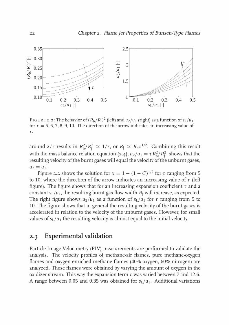
FIGURE 2.2: The behavior of (Rb/Rj)2 (left) and u2/u1 (right) as a function of sL/u1
for τ = 5, 6, 7, 8, 9, 10. The direction of the arrow indicates an increasing value ofτ .
around 2/τ results in R2b/R2
j ≃ 1/τ , or Rj ≃ Rbτ1/2. Combining this result
with the mass balance relation equation (2.4), u2/u1 = τ R2b/R2
j , shows that the
resulting velocity of the burnt gases will equal the velocity of the unburnt gases,
u2 = u1.
Figure 2.2 shows the solution for x = 1 − (1 − C)1/2 for τ ranging from 5to 10, where the direction of the arrow indicates an increasing value of τ (leftfigure). The figure shows that for an increasing expansion coefficient τ and a
constant sL/u1, the resulting burnt gas flow width Rj will increase, as expected.
The right figure shows u2/u1 as a function of sL/u1 for τ ranging from 5 to
10. The figure shows that in general the resulting velocity of the burnt gases isaccelerated in relation to the velocity of the unburnt gases. However, for small
values of sL/u1 the resulting velocity is almost equal to the initial velocity.
2.3 Experimental validation
Particle Image Velocimetry (PIV) measurements are performed to validate the
analysis. The velocity profiles of methane-air flames, pure methane-oxygen
flames and oxygen enriched methane flames (40% oxygen, 60% nitrogen) areanalyzed. These flames were obtained by varying the amount of oxygen in the
oxidizer stream. This way the expansion term τ was varied between 7 and 12.6.A range between 0.05 and 0.35 was obtained for sL/u1. Additional variations

2.3. Experimental validation 23
Nd:YAG laser Optics
Flame
Burner
Camera
Computer
FIGURE 2.3: Schematic PIV set-up consisting of a Nd:YAG laser, CCD camera, opticsand burner.
for both terms were accomplished by varying the equivalence ratio φ and the
unburnt gas velocity u1.
Figure 2.3 shows a schematic of the PIV set-up. A laser beam with a wave-length of 532 nm from a double Quantel-Brio Nd:YAG laser with a pulse du-
ration of 5 ns, a repetition rate of 10 Hz and an energy of 60 mJ per pulse
illuminated the seeding particles carried along with the gas flow. A Roper Sci-
entific ES 1.0 CCD camera was used to record the movement of the particles.
The premixed gas mixture was supplied to the burner using a mixing panelwith Mass Flow Controllers (MFCs), which were set and monitored using an
interface to a PC. For the methane-air flame, a conical nozzle with a top diame-
ter of 12.5 mmwas used in order to ensure a plug flow of unburnt gases exiting
the burner, see figure 2.3. A pilot burner with an exit diameter of 1.7 mm wasused for the experiments with the methane-oxygen flame.
The equivalence ratio of themethane-air flame was varied between 0.90 and
1.30. With the one-dimensional numerical flame code Chem1D [14] the values
of the expansion term τ and burning velocity sL were calculated using the GRI-
mech 3.0 mechanism, see table 2.1. Measurements with the methane-oxygenflame were only performed for a stoichiometric mixture. The expansion term
and burning velocity for this flame were calculated with Chem1D as well. The
values are equal to 12.6 and 3.09 m/s, respectively. Aluminum-oxide particles

24 Chapter 2. Flame Jet Properties of Bunsen-Type Flames
TABLE 2.1: Expansion term τ and burning velocity sL for different equivalence ratiosfor a methane-air flame.O2 = 0.21 φ [-]
0.90 0.95 1.00 1.10 1.20 1.30τ [-] 7.1 7.3 7.5 7.4 7.1 6.8
sL [m/s] 0.325 0.358 0.367 0.367 0.333 0.250
Distance
above
burner
nozzle[m
m]
Radial distance [mm]
5 10
15
20
25
30
35
−10 −5 0
5
10
FIGURE 2.4: Measured velocity field of a methane-air flame with u1 = 1.1 m/s, Rb =12.5 mm and φ = 0.90. For illustrative purposes, arrays of arrows of the velocities ofthe unburnt and burnt gases are highlighted.
were used as seeding for the PIV measurements with the methane-air flames.
Different velocities of the unburnt gases of 1.1, 1.6 and 2.1 m/s were set to
vary the ratio between the burning velocity and the unburnt gas velocity sL/u1.Magnesium-oxide particles were used for the methane-oxygen flames and the
velocities were set to 35, 40, 45, 50 and 55 m/s. The velocity fields were analyzed
using PIVview2C [50].

2.3. Experimental validation 25
Distance
above
burner
nozzle[m
m]
Radial distance [mm]
2
4
6
8
10
12
−2 0 2
FIGURE 2.5: Measured velocity field of a methane-oxygen flame with u1 = 40 m/s,Rb = 1.7 mm and φ = 1.00. For illustrative purposes, arrays of arrows of the velocitiesof the unburnt and burnt gases are highlighted. The flame front is highlighted as well.
Figure 2.4 and 2.5 show typical velocity fields of a methane-air flame and
a methane-oxygen flame measured with PIV. Both pictures show a flow of un-
burnt gases exiting the burner nozzle which approaches a plug flow with asmall viscous boundary layer at the edges. Figure 2.4 shows that because of
the acceleration of the velocity component normal to the flame front after ex-
pansion, the gases flow sideways causing a dip in the velocity field above the
flame tip. The resulting flow of burnt gases therefore is not a perfect plug flow.The velocity of the burnt gases u2 is averaged over the flame tube. The edge
of the flame tube width is defined as the half-maximum velocity points of the
downstream jet. Comparison between the measurements and theoretical re-
sults for the methane-air flame (τ ≃ 7.0 − 7.4) are shown in figure 2.6 (left).
The error bars have been obtained by using the velocity data of one extra datapoint compared with the chosen flame tube width, i.e. effectively increasing
the flame tube width, and by using the velocity data of one data point less, i.e.
decreasing the flame tube width. The figure shows a good agreement between

26 Chapter 2. Flame Jet Properties of Bunsen-Type Flames
sL/u1 [-]
u2/u
1[-]
1.2
1.3
1.4
1.5
1
1.1
0.15 0.2 0.25 0.3 0.35
τ = 7.0
τ = 7.4
sL/u1 [-]
u2/u
1[-]
0.9
0.95
1
1.05
1.1
1.15
0.05 0.06 0.07 0.08 0.09
τ = 12.6
FIGURE 2.6: The ratio of the burnt and unburnt gas velocity u2/u1 as a functionof sL/u1 for the methane-air flames (left) and the methane-oxygen flames (right).Theoretical results are depicted by the asterisks, the measurements by the circles.Theoretical results for the complete range for τ = 7.0, τ = 7.4 and τ = 12.6 arerepresented by the continuous lines.
the theoretical and experimental results.
As the burning velocity sL of a methane-oxygen flame is very small com-pared to the unburnt gas flow u1, the burnt gases only just diverge sideways
after the expansion, see figure 2.5. Therefore the dip in the velocity field above
the flame tip is a lot smaller and the resulting flow is closer to a perfect plug
flow. The values of the measured u2 are compared with the theoretical result
for u2 in figure 2.6 (right, τ ≃ 12.6). It is interesting to note that, althoughmost gases experience a sudden velocity jump over the flame front, this is not
so intense for the methane-oxygen flame. This is because, as already stated, the
burning velocity sL is very small compared to the unburnt gas flow u1. There-
fore the parallel velocity component to the flame front, which remains constantafter the flame front, dominates the resulting total velocity after the flame front.
Again, theoretical and experimental results show good agreement.
The results of the PIVmeasurements with themethane-air flame andmeth-
ane-oxygen flame seem to confirm the theory presented in section 2.2. How-
ever, it is expected that deviations occur if the flame part in the tip responsiblefor the velocity dip becomes relatively large compared to the length of the flame
front. This is shown by the following measurements where the velocities of an
oxygen enriched methane-air flame are analyzed.

2.4. Discussion 27
TABLE 2.2: Expansion term τ and burning velocity sL for different equivalence ratiosfor an oxygen enriched methane-air flame (40% oxygen in oxidizer stream).
O2 = 0.40 φ [-]
0.70 0.80 0.90 1.00 1.10 1.20 1.30τ [-] 8.6 9.0 9.3 9.6 9.8 10.0 10.0
sL [m/s] 0.971 1.113 1.203 1.242 1.230 1.167 1.054
The same conical burner was used as for the methane-air flame, but now an
extra nozzle with an inner diameter of 5 mm was placed on top to stabilize the
flame. The amount of oxygen in the oxidizer stream was set to 40%, causing an
increase of the burning velocity sL and the expansion term τ . The equivalence
ratio was varied between 0.7 and 1.3. The corresponding burning velocitiesand flame temperatures were calculated with Chem1D using the GRI-mech
3.0 mechanism, see table 2.2. Aluminum-oxide particles were used as seeding
and the velocities of the unburnt gases were set to 7.2, 8.4 and 9.5 m/s.
Figure 2.7 shows a typical velocity field of the oxygen enriched methane-air flame. A clear plug flow of unburnt gases exits the burner nozzle. The
burnt gases flow sideways after the expansion over the flame front just like for
the case of the methane-oxygen flame, only the effect is considerably stronger.
This is resulting in a larger velocity dip above the flame tip. The difference
with the model is still only 10%. However, since the influence of this velocitydip causes a decrease in the averaged velocity of burnt gases, this leads to a
systematic deviation from the theoretical results, see figure 2.8. In fact, the
averaged velocity of the burnt gases is smaller than the velocity of the unburnt
gases for most measurements. The trend of the experimental results howeverseems to be in accordance with the theoretical results. To validate the PIV
results, we checked and verified mass conservation for the three flame types.
2.4 Discussion
It was shown in figure 2.5 that the burnt gases of the methane-oxygen flameonly slightly diverge after expansion over the flame front. Therefore, the dip
in the velocity field above the flame tip is small. The dip of the velocity field
above the flame tip of the methane-air flame is also small, although there is a

28 Chapter 2. Flame Jet Properties of Bunsen-Type Flames
Distance
above
burner
nozzle[m
m]
Radial distance [mm]
5
10
15
20
25
−5 0 5
FIGURE 2.7: Measured velocity field of the oxygen enriched methane-air flame withu1 = 7.2 m/s, Rb = 5.0 mm and φ = 1.00. For illustrative purposes, arrays of arrowsof the velocities of the unburnt and burnt gases are highlighted.
strong divergence of the burnt gases after the flame front, shown in figure 2.4.
The relatively large surface area of the flame front and therefore the amount
of burnt gases along the flame front, however, diminishes the influence of thedivergence of the burnt gases at the flame tip.
The divergence of the burnt gases of the oxygen enrichedmethane-air flame,
shown in figure 2.7, is approximately the same as the divergence of the burnt
gases of the methane-air flame. However, the burning velocity sL of the oxygenenriched methane-air flame is much higher. Although it seems that this flame
is an intermediate between the methane-air flame and the methane-oxygen
flame, it actually is very different realizing that the amount of flame surface
in the tip region has a significant contribution to the overall flame area. The
flame front surface can not compensate the effect of the strong divergence ofthe burnt gases at the flame tip in this case. This leads to the systematic error
observed. A solution to this problem could be to stabilize the oxygen enriched
methane-air flame on a burner with a larger nozzle diameter, resulting in a

2.5. Conclusions 29
sL/u1 [-]
u2/u
1[-]
0.8
0.9
1
1.1
0.1 0.12 0.14 0.16 0.18 0.2
τ = 9
FIGURE 2.8: The ratio of the burnt and unburnt gas velocity u2/u1 as a function ofsL/u1 for the oxygen enhanced methane-air flames. Theoretical results are depictedby the asterisks, the measurements by the circles. Theoretical results for the completerange for τ = 9 are represented by the continuous line.
larger flame front area. However, this is not easy for these flames which aresensitive to flash-back in case of larger burners.
Inaccuracies may also occur because boundary layer effects are not taken
into account. The different flow behavior of the burnt gases at the edge of the
burner nozzle may cause deviations from themodel. The same argument holds
for the flame tip, where the influence of the flame curvature was not taken intoaccount.
2.5 Conclusions
In this chapter a simple relation is presented which predicts the parametersof the burnt gas flow of a flame jet of a Bunsen type flame after expansion
over the flame front. These parameters of the burnt gas flow, namely the jet
velocity and jet width, are important to calculate or estimate the heat transfer

30 Chapter 2. Flame Jet Properties of Bunsen-Type Flames
from flame jets to products. This model is based on an idealized representation
of the flame and flow characteristics. Only the global conservation equations ofmass, momentum and energy are taken into account. Effects like flame stretch
and flame curvature are not considered in the derivation. Therefore this work
should be considered as a first step in this area. Here we investigate the range of
applicability of this simple model and which modifications are to be expected.PIVmeasurements have been performed on flames with different amounts
of oxygen in the oxidizer stream, equivalence ratios and unburnt gas velocities,
in order to validate the results of the model for a wide range of parameter set-
tings. Measurements on a methane-air and a methane-oxygen flame show a
good agreement with the model. It is striking to see, that although unburntgases experience a velocity jump over the flame front, this is not the case for
the methane-oxygen flame. However, deviations from the predictions based on
the theoretical model occur, when the amount of flame area in the tip region
becomes relatively large compared to the overall dimensions of the flame. This
was the case for an oxygen enhanced methane-air flame, where the resultingvelocity of the flame jet showed a systematic deviation from the results of the
model. This effect could be minimized by performing the experiments for this
flame type with a burner with a larger burner nozzle diameter. This way the
tip area is smaller compared to the overall dimensions of the flame and thedivergence of the burnt gases at the flame tip will have a smaller effect on the
total flow behavior of the burnt gases after the flame front. Further experiments
have to be performed to investigate this effect.
Chapter
3Heat transfer from animpinging laminar flame jet toa flat plate
3.1 Introduction
Flame-impingement heating is a frequently employed method to enhance the
heat transfer to a surface. Often the burners are supplied with a pure fuel andoxygen mixture to enhance the heat transfer. When the convective heat flux has
to be determined, these flames can be treated as hot inert jets. This approach
is plausible because the flow behavior of flame jets and hot isothermal jets
is comparable, as explained in chapter 1. The main difference between the
oxy-fuel flames and the hot inert jets is that the flames contain a lot of freeradicals as a result of dissociation of stable molecules like H2O and CO2 at
high temperatures. These free radicals recombine in the cold boundary layer
releasing extra heat. A correction which takes these chemical reactions and the
resulting extra heat input into account has to be performed afterwards to obtainthe total heat transfer.
Simple analytical expressions for the heat transfer of inert jets are very use-
ful from an engineering point of view when the heat transfer needs to be esti-
mated. Sibulkin derived a semi-analytical relation for the laminar heat transfer
of an impinging flow to a body of revolution [61]. This relation has been the ba-sis of most other experimental and theoretical results since [60, 30, 36, 9, 34].
An important limitation of this relation, however, is that it is only applicable
for large nozzle-to-plate spacings. Nevertheless, a smaller spacing becomes
31
32 Chapter 3. Heat transfer from a laminar flame jet to a flat plate
very interesting when the heat flux needs to be increased. Furthermore, for the
limit of non-viscous flows an unrealistic heat transfer is predicted using thismodel.
In this chapter we present an analytical solution for the convective heat
transfer of an impinging flame jet to the hot spot of a flat plate. In the first
section we will concentrate on the solution for the case that the plate is placedclose to the flame tip. The solution consists of two parts. A solution is obtained
for the small viscous boundary layer close to the plate. The other solution ap-
plies for the region further away from the plate where viscosity is not dominant
anymore. The two solutions will be linked together at the edge of the boundary
layer. The result will be validated with numerical calculations in the subse-quent section. Using the results of the numerical calculations, an extension of
the analytical solution of the heat flux can be made, so it will be applicable for
larger distances between the flame tip and the plate as well. This will be shown
in section 3.4, followed by some conclusions in section 3.5.
3.2 Analytical solution for the heat transfer for small spac-
ings
Figure 3.1 shows a schematic overview of a premixed stagnation flame imping-
ing normal to a plane surface. From this figure, we can distinguish the flame
region, the free jet region, the stagnation region and the impingement surface.
Cremers [16] has shown that since the typical time scales of the regions are
different, the regions can be decoupled, treated separately and coupled after-wards again. If the plate is placed close to the flame, the flame front and the
stagnation boundary layer will interact and decoupling of the regions is not al-
lowed anymore; the resulting error of the predicted heat flux, however, is only
10% at most [18]. In this chapter, we will focus on the free jet region and thestagnation region to calculate the heat flux from the flame to the hot spot of
the plate, which has a width of 2Rj. For a flame where pure oxygen is supplied
to the oxidizer stream, it was shown in chapter 2 that the burnt gases form a
flow profile very close to a plug flow after the flame front. The velocity of the
burnt gases rapidly drops at the edges of the stream tube. The resulting plugflow velocity U [m/s] and plug flow jet radius Rj [m], which can be calculated
using the unburnt gas parameters [55], will be used as input parameters for the
model.

3.2. Analytical solution for the heat transfer for small spacings 33
Flame front
Burner
Impingement
surface
H
URj
x, u
r, v
FIGURE 3.1: Schematic overview of a stagnation flame impinging to a plane surface.
In literature often the distance from the burner to the impingement surface
is used as an independent parameter. However, using different fuels while
keeping the unburnt gas velocity constant results in different flame heights
because of the different burning velocities. Therefore, if the distance from theburner to the plate is kept constant, the distance from the flame tip to the plate
H [m] will vary for the different fuels. For this reason, we choose the distance
from the flame tip to the plate H as an input parameter, instead of the distance
from the burner to the plate.First we will consider the case where the plate is positioned close to the
flame tip, H ≤ Rj. A hot inert plug flow with velocityU and burnt gas jet radius
Rj, which is formed after the flame front, impinges on the plate. The system
now is reduced to a steady one-dimensional problem and behaves as a potential
flow far from the surface. A thin boundary layer of thickness xδ is formed closeto the surface. The heat-transfer processes induce a fast temperature change
in the boundary layer. We will analyze the system by studying the transport
equations in both regions and coupling the solutions at the edge of the regions.

34 Chapter 3. Heat transfer from a laminar flame jet to a flat plate
The conservation equations of mass and momentum are given by:
∂ρ
∂ t+ ∇ · (ρv) = 0, (3.1)
∂(ρv)
∂ t+ ∇ · (ρvv) = −∇ · P + ρg, (3.2)
where g is the gravitational vector [m/s2] and the tensor P is a short-hand nota-tion for P = pI + τ . Furthermore, p is the hydrostatic pressure [Pa], I the unittensor and τ the stress tensor [kg/(m·s2)].
Often the Richardson number Ri is used to determine the importance of
buoyancy in the flow. The Richardson number is a dimensionless number that
expresses the ratio of potential to kinetic energy. Since Ri = O(10−5) in thiscase, the effect of buoyancy is neglected. The jet is inert, since we approximate
the flame jet by a hot isothermal jet and take no chemical recombination into
account. To calculate the total heat flux, the convective heat flux can simply be
multiplied by a factor which takes the thermochemical heat release into account[16]. Since the core region of the jet flow is essentially one-dimensional, the
temperature is a function of the spatial coordinate x only, so T = T (x) and
therefore ρ = ρ(x). Assuming an incompressible flow and using the ideal gas
law p = ρRT , ρT is a constant. Since the velocity profile is a plug flow, the
velocity component u is a function of x only. Using m = ρu and v = r · v(x),the continuity equation now yields
dm
dx= −ρK , (3.3)
where K , the strain rate of the mixture [1/s], is a function of x only and equalto K = 2v = 2∂v/∂r .
If p = p(x, r) and µ = µ(x), the equations for x - and r -momentum be-
come [32, 62]:
−mdu
dx+ d
dx
[
2
3µ
(
2du
dx− K
)]
+ µ
2
dK
dx= ∂p
∂x, (3.4)
mdK
dx+ 1
2ρK 2 − d
dx
(
µdK
dx
)
= −2
r
∂p
∂r, (3.5)
with µ the dynamic viscosity [kg/(m·s)]. It can be seen from equation (3.4),
that the pressure derivative ∂p/∂x is a function of x only. Differentiation of
3.2. Analytical solution for the heat transfer for small spacings 35
equation (3.4) with respect to r and changing the order of differentiation then
gives that ∂p/∂r is a function of r only. From equation (3.5) it then follows that−2∂p/(r∂r) is a constant, i.e.
mdK
dx− d
dx
(
µdK
dx
)
= J − 1
2ρK 2, (3.6)
with J = −2∂p/(r∂r). The strain rate K increases as the flow approaches the
plate to a maximum at the plate for non-viscous flows. For viscous flows the
maximum strain rate is a bit smaller due to the viscous boundary layer than
for non-viscous flows. Now the maximum strain rate can be found just beforethe plate. At the plate, the strain rate will be equal to zero. If we define the
maximum strain rate a = Kmax [1/s], for non-viscous flows J becomes equal to
ρba2/2, with ρb the density of the burnt gases. For viscous flows J will not be
equal to ρba2/2, but the difference is assumed to be small.
Equation (3.6) can not be solved analytically for the whole domain −H <
x < 0, where x = −H is the position of the flame tip and x = 0 is the hot side
of the plate. An analytical solution can be obtained, however, if we decouple
the domain in a region far from the plate to the viscous boundary layer, −H <
x < −xδ, and a region consisting of the viscous boundary layer, −xδ < x < 0.The resulting solutions for the velocity profiles in both regions will be linked at
x = −xδ, where K = a.The order of magnitude for the terms of equation (3.6) far from the plate
can be estimated using O(x) = H and O(K ) = U/H :
O
(
ρU 2
H 2
)
+ O
(
µU
H 3
)
= O(
ρa2)
+ O
(
ρU 2
H 2
)
. (3.7)
Since O(a) = U/H , it is easy to see that the viscous term is not relevant farfrom the plate if H ≫ √
ν/a, where ν = µ/ρb is the kinematic viscosity [m2/s].
Far from the plate the density is constant. Using the continuity equation
(3.3), the relation between the strain rate K and the velocity u becomes:
K = −du
dx. (3.8)
Using equation (3.8), equation (3.6) is now reduced to:
−uu′′ = 1
2a2 − 1
2u′2. (3.9)

36 Chapter 3. Heat transfer from a laminar flame jet to a flat plate
The solution for this equation can be obtained analytically. The boundary con-
ditions at x = −H are u = U and K = −du/dx = 0. Using these boundaryconditions, the following solutions for the velocity profile and strain profile can
be found:
u(x) = − a2
4U(x + xref)
2 − a(x + xref), (3.10)
K (x) = a2
2U(x + xref) + a, (3.11)
where a = 2U/H and the value of xref is determined by the boundary layerthickness xδ. Equations (3.10) and (3.11) are valid for −H < x < −xδ, but also
for the whole domain if the flow is non-viscous (xref = 0).Close to the plate m and K become zero and equation (3.6) is reduced for
−xδ < x < 0 to
− d
dx
(
µdK
dx
)
= 1
2ρba2, (3.12)
indicating a quadratic behavior as function of x for K in the viscous bound-ary layer. In this region, the density and velocity of the burnt gas flow can be
approximated by
ρ ∼ ρ0 + ρ ′x, u ∼ bx2,
with ρ0 the density of the burnt gas flow at the hot side of the plate and b a
constant. Equation (3.8) still holds, since
ρdu
dx∼ 2bρ0x, u
dρ
dx∼ bρ ′x2,
and therefore ρdu/dx ≫ udρ/dx . Now, using K (0) = 0 and K (−xδ) = a ≃2U/H , the solution for the velocity profile in the viscous boundary layer be-comes
u(x) = axδ
(
x3
3x3δ
+ x2
x2δ
)
, (3.13)
with xδ = 2√
ν/a. The velocity profile far from the plate (3.10) will be coupled
to the velocity profile in the viscous boundary layer (3.13) at x = −xδ, whereK = a = 2U/H . Equation (3.10) for −H < x < −xδ now becomes:
u(x) = − a2
4U(x + xδ/3)2 − a(x + xδ/3). (3.14)

3.2. Analytical solution for the heat transfer for small spacings 37
Convection and Thermochemical Heat Release are the main heat-transfer
mechanisms for impinging oxy-fuel flame jets. To calculate the convective con-tribution, the conservation equation of energy for the burnt gasses close to the
heated side of the plate is reduced to a balance of conduction and convection:
ρucpdT
dx= d
dx
(
λdT
dx
)
, (3.15)
where cp is the heat capacity of the burnt gas flow [J/(kg·K)] and λ the conduc-
tivity coefficient [W/(m·K)]. Substituting the equations for the velocity u (3.13)
and (3.14) results in relations for the heat transfer from the burnt gas flow tothe glass product.
First we determine the heat transfer for a non-viscous gas flow (xδ = 0).We assume both λ and the thermal diffusivity α = λ/(ρcp) [m
2/s] to be con-
stant. Numerical calculations have shown that this assumption is valid. After
substituting q = λdT/dx , the conservation equation of energy (3.15) changesto:
0∫
s
dq
q= 1
α
0∫
s
udx, (3.16)
which after integration results in the following equation for q:
q(s) = q0 exp
− 1
α
0∫
s
udx
. (3.17)
Now we introduce the Peclet number, a dimensionless parameter giving the ra-tio of heat transfer by convection and conduction. The Peclet number is defined
as:
Pe = U H
α. (3.18)
Equation (3.17) can be made dimensionless using x ′ = x/H . After integration
over the whole domain −H < x < 0 and substituting equation (3.14) for the
velocity profile u, the solution for the non-viscous heat transfer from the burnt

38 Chapter 3. Heat transfer from a laminar flame jet to a flat plate
gases to the plate q0 is given by
q0 = λdT
dx
∣
∣
∣
0= λ(T0 − Tflame)
0∫
−Hexp
[
− 1α
0∫
sudx
]
ds
(3.19)
= λ(T0 − Tflame)
H0∫
−1exp
[
−Pe(
13 x ′3 + x ′2
)]
ds ′. (3.20)
If we take viscosity into account to calculate the heat flux q0, we have to
make the distinction between the burnt gas flow region and the viscous bound-
ary layer again to calculate the denominator of equation (3.19). The denomina-
tor of equation (3.19) now becomes equal to
0∫
−H
exp
− 1
α
0∫
s
udx
ds =0∫
−xδ
exp
− 1
α
0∫
s
u2dx
ds+
−xδ∫
−H
exp
− 1
α
−xδ∫
s
u1dx +0∫
−xδ
u2dx
ds, (3.21)
where the velocity profile in the burnt gas flow region u1 is given by equation
(3.14) and the velocity profile in the viscous boundary layer u2 by equation (3.13).
Implementing these velocity profiles in equation (3.21) and making this equa-tion dimensionless, results in the following denominator for equation (3.19) for
the viscous situation:0∫
−H
exp
− 1
α
0∫
s
udx
ds =H
0∫
−xδ/H
exp
1
12
Pe2
Prx ′4 +
√
4
18
Pe3
Prx ′3
ds ′+
H
−xδ/H∫
−1
exp
[
−Pr − Pe
(
1
3x ′3 + 1
3
√
2Pr
Pex ′2+
1
9
2Pr
Pex ′ + 1
9
√
2Pr
Pe
3
+ x ′2+
2
3
√
2Pr
Pex ′ − 1
3
2Pr
Pe
)]
ds ′, (3.22)
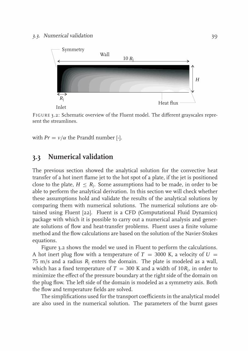
3.3. Numerical validation 39
SymmetryWall
InletHeat flux
Rj
Rj
10
H
FIGURE 3.2: Schematic overview of the Fluent model. The different grayscales repre-sent the streamlines.
with Pr = ν/α the Prandtl number [-].
3.3 Numerical validation
The previous section showed the analytical solution for the convective heat
transfer of a hot inert flame jet to the hot spot of a plate, if the jet is positioned
close to the plate, H ≤ Rj. Some assumptions had to be made, in order to beable to perform the analytical derivation. In this section we will check whether
these assumptions hold and validate the results of the analytical solutions by
comparing them with numerical solutions. The numerical solutions are ob-
tained using Fluent [22]. Fluent is a CFD (Computational Fluid Dynamics)
package with which it is possible to carry out a numerical analysis and gener-ate solutions of flow and heat-transfer problems. Fluent uses a finite volume
method and the flow calculations are based on the solution of the Navier-Stokes
equations.
Figure 3.2 shows the model we used in Fluent to perform the calculations.A hot inert plug flow with a temperature of T = 3000 K, a velocity of U =75 m/s and a radius Rj enters the domain. The plate is modeled as a wall,
which has a fixed temperature of T = 300 K and a width of 10Rj, in order to
minimize the effect of the pressure boundary at the right side of the domain on
the plug flow. The left side of the domain is modeled as a symmetry axis. Boththe flow and temperature fields are solved.
The simplifications used for the transport coefficients in the analytical model
are also used in the numerical solution. The parameters of the burnt gases

40 Chapter 3. Heat transfer from a laminar flame jet to a flat platereplacements
Differen
tmassequationterm
s
Distance to the plate [m]
−1000
0
1000
2000
3000
4000
5000
6000
7000
−4 −3 −2 −1 0
×10−3
FIGURE 3.3: The terms −ρ ∂u∂x (solid line) and u ∂ρ
∂x (dashed line) plotted against thedistance to the plate x , with U = 75 m/s, T = 3000 K, H = 4 mm and Rj = 20 mm.
are chosen to be constant with ρ = ρb = 0.083 kg/m3, cp = 2000 J/(kg·K),µ = 5.6 · 10−5 kg/(m·s) and λ = 0.16 W/(m·K). The values for cp, λ and
µ are chosen at a temperature of 1500 K using the transport data documented
by Kee and Miller [31] and the thermodynamic data from the GRI-mech 3.0mechanism.
First we check whether the strain rate K , defined by equation (3.3), can
be simplified according to equation (3.8). Therefore u∂ρ/∂x should be signifi-
cantly smaller than ρ∂u/∂x . Figure 3.3 shows both terms as a function of thedistance to the plate. For this particular calculation a temperature dependent
density was used, namely ρ = 1.1 · (T/298)−1.06 [14]. The figure shows that far
from the plate u ∂ρ
∂x = 0. Closer to the plate u ∂ρ
∂x is not negligible anymore, but
ρ ∂u∂x still is the leading term. Therefore, the assumption seems to hold.
The analytical solution for the velocity of the burnt gases was obtained bysolving the momentum equation in r -direction. Therefore a distinction was
made between the burnt gas region far from the plate where the diffusivity
term was neglected and the viscous boundary layer where the convection term

3.3. Numerical validation 41replacements
Differen
tmomen
tum
equationterm
s
Distance to the plate [m]
−8
−6
−4
−4
−2
−2
0
2
4
6
8
−3 −1 0
×107
×10−3
FIGURE 3.4: The separate terms of equation (3.6). The solid line represents the con-
vection term m dKdx , the dotted line the diffusion term d
dx
(
µ dKdx
)
, the dashed line the
source term ρK 2 and the dashed-dotted line the constant term ρba2, with U = 75 m/s,T = 3000 K, H = 4 mm and Rj = 20 mm.
and the source term were assumed to approach zero. In figure 3.4 the separate
terms of equation (3.6) are plotted against x . Far from the wall, the viscous termindeed is not relevant and therefore there is a balance between the convection
term, the source term and the constant ρba2. Very close to the wall, the con-
vection term and the source term become zero and the negative diffusion term
equals the constant ρba2. The solutions for the velocity profiles far from thewall and in the viscous boundary layer close to the plate were linked together at
x = −xδ, which is approximately at x = −0.2 mm. At x = −xδ there is a bal-
ance between the four terms, which is not taken into account in the derivation
of the analytical solution. The results of the numerical calculations will show
whether this approximation has a big influence on the velocity profile.Equations (3.13) and (3.14) represent the analytical solution for the veloc-
ity profile from the symmetry axis up to close to the edge of the stream tube
when H < Rj. Figure 3.5 shows a comparison between this analytical solution

42 Chapter 3. Heat transfer from a laminar flame jet to a flat platereplacements
Velocity[m
/s]
Distance to the plate [m]
0
10
20
30
40
50
60
70
80
−2 −1.5 −1 −0.5 0
×10−3
FIGURE 3.5: Velocity profile over the symmetry boundary, with U = 75 m/s, T =3000 K, H = 2 mm and Rj = 20 mm. The dashed line represents the analyticalcalculation, the solid line represents the numerical results.
(dashed line) and the numerical results obtained with Fluent (solid line). The
analytical equations for the velocity profile correspond very well to the numeri-cal calculations.
Equation (3.20) represents the convective heat flux from the inert flame jet
to the hot spot for the non-viscous case. The heat flux for the viscous case can
be calculated using equations (3.19) and (3.22). The temperature profile over
the symmetry axis is calculated with Fluent. The resulting heat flux to the hot
spot, using q = λ ∂T∂x
∣
∣
∣
0, can be compared with the analytical solution. The heat
transfer is calculated for different Prandtl numbers Pr, ranging from 0 (non-
viscous flow) to 1.The ratio of the analytically calculated heat flux and the non-viscous heat
flux as a function of Pr is depicted using dots in figure 3.6. The asterisks repre-sent the ratio of the numerically calculated heat flux and the non-viscous heat
flux as a function of Pr. Therefore a distance to the plate of H = 2 mm and a
plug width of Rj = 20 mm are chosen. For a Prandtl number of 0, the ratio be-

3.3. Numerical validation 43
replacements
q(P
r)/q n
onvisc[-]
Pr [-]
0.7
0.75
0.8
0.85
0.9
0.95
1
1.05
0 0.2 0.4 0.6 0.8 1
FIGURE 3.6: The ratio of the viscous heat flux and non-viscous heat flux as a functionof the Prandtl number. The dots represent the analytical results, the asterisks thenumerical results; U = 75 m/s, T = 3000 K, H = 2 mm, Rj = 20 mm.
tween the viscous heat transfer and non-viscous heat transfer should be equal
to 1. A small deviation can be observed for the numerical results. For increas-
ing Prandtl number, the heat transfer should decrease due to an increasing
viscous boundary layer thickness. A good agreement can be observed between
the analytical and numerical results.It is expected that the heat transfer to the plate shows a fast decay out-
side the hot spot, which has a width of 2Rj. Also, the heat flux within the hot
spot will decrease with increasing distance from the symmetry plane due to the
gases which flow radially outwards. To check the validity range of the analyticalequations for the heat flux (3.19) and (3.22), the local heat flux over the entire
plate is calculated using Fluent.
Figure 3.7 shows the ratio of the numerically calculated local heat flux and
the analytical heat flux at the hot spot as a function of the normalized distance
to the symmetry axis r/Rj. The ratio of the numerical and analytical heat fluxis equal to 1 at the symmetry axis. A small decrease can be observed with
increasing distance from the symmetry plane to the edge of the hot spot at a
normalized distance of r/Rj = 1. The heat transfer decreases fast outside the

44 Chapter 3. Heat transfer from a laminar flame jet to a flat plate
q numerical/q a
nalytical[-]
r/Rj [-]
r = Rj0.2
0.4
0.6
0.8
1
00 2 4 6 8 10
FIGURE 3.7: Ratio of the numerically calculated heat flux and the analytical heat fluxat the hot spot as a function of r/Rj.
hot spot. Therefore, the analytical solutions for the heat flux seem to hold forthe hot spot region.
3.4 Extension of the solution for the heat transfer to large
spacings
So far we derived the convective heat flux from a hot inert jet to the hot spot
of the plate if the plate is positioned close to the jet, H < Rj. It was observed
that the maximum strain rate a = Kmax just before the plate determines theheat flux. For small flame tip to plate distances, the strain rate is given by
a = 2U/H . Increasing the gas velocity U or decreasing the distance from
the flame tip to the plate H will result in a larger strain rate. Because of the
increased strain rate, the boundary layer will be thinner and therefore the heat
flux will be increased.Increasing the distance from the flame tip to the plate H while keeping the
gas velocity U constant will have the opposite effect. The strain rate decreases
and therefore the heat flux will decrease as well. From a certain distance from

3.4. Extension of the solution for the heat transfer to large spacings 45
Velocity
[m/s]
Distance to the plate [m]
0
10
20
30
40
50
60
70
80
−4 −3 −2 −1 0 1
×10−3
FIGURE 3.8: Velocity profiles over the symmetry boundary, for the solid line H =4 mm, for the dashed line H = 3 mm, for the dashed-dotted line H = 2 mm and forthe dotted line H = 1 mm.
the flame tip to the plate, however, the boundary layer will reach its maximum
thickness and the maximum strain rate will remain constant. The maximumstrain rate is no longer equal to a = 2U/H from this point on. This effect is
visualized in figure 3.8. This figure shows the velocity profiles over the sym-
metry plane for a plug flow with radius Rj = 0.5 mm and an increasing flame
tip to plate distance from 1 to 4 mm. Increasing the distance from H = 1 (dot-ted line) to 2 mm (dashed-dotted line) results in a thicker boundary layer and
therefore a smaller strain rate. Increasing the distance to H = 3 mm only has
little effect on the velocity profile, while increasing the distance from H = 3 to
4 mm has no effect at all. Therefore, increasing the distance to the plate has
no effect on the velocity profiles for high H/Rj ratios and the strain rate willremain constant. We will show in this section how the strain rate and there-
fore the heat flux alters for the case that H > Rj using the results of Fluent
calculations.

46 Chapter 3. Heat transfer from a laminar flame jet to a flat plate
aH
/(2
U)[-]
H/Rj [-]
20
15
10
5
00 5 10 15 20 25 30
FIGURE 3.9: Relation between aH/(2U) and H/Rj; the dots represent the numericalcalculations, the solid lines the functions aH/(2U) = 1 and aH/(2U) = 18H/(30Rj).
The numerical effect of the ratio H/Rj on the maximum strain rate a is
shown in figure 3.9. The factor aH/(2U) is plotted as a function of H/Rj.
This factor is equal to 1 for small values of H/Rj; this is in agreement withthe analytical solution. Keeping the distance to the plate H and the burnt gas
velocityU constant and decreasing the plug flow radius Rj results in an increase
of the effective strain rate a. Furthermore, for a H/Rj ratio of 4 and higher
and a constant plug flow radius Rj and burnt gas velocity U , the distance tothe plate H has no influence on the strain rate a. The strain rate a now is a
constant, represented by the straight line indicating that aH/(2U) ∼ H/Rj or
a = 6U/(5Rj) independent of H .
We can now adjust equation (3.22) to make it valid not only for H/Rj < 1but for the complete H/Rj range. The two straight lines in figure 3.9 intersectat H/Rj = 5/3. Since the strain rate is independent of the distance H for
a ratio of H/Rj larger than 5/3, the strain rate for large H/Rj ratios can be
defined as a = 6U/(5Rj) = 2U/H∗. The critical distance H∗ is defined here as

3.4. Extension of the solution for the heat transfer to large spacings 47
H∗ = 5Rj/3. Equation (3.22) now can be written as:
2
0∫
−H∗
exp
− 1
α
0∫
s
udx
ds =H∗0∫
−xδ/H∗
exp
1
12
Pe2
Prx ′4 +
√
4
18
Pe3
Prx ′3
ds ′+
H∗−xδ/H∗∫
−1
exp
[
−Pr − Pe
(
1
3x ′3 + 1
3
√
2Pr
Pex ′2+
1
9
2Pr
Pex ′ + 1
9
√
2Pr
Pe
3
+ x ′2
+2
3
√
2Pr
Pex ′ − 1
3
2Pr
Pe
)]
ds ′,
(3.23)
with
H∗ ={
H for H < 5Rj/35Rj/3 for H ≥ 5Rj/3
, (3.24)
and Pe = U H∗/α. A derivation of the convective heat flux from an impinging
flame jet to a flat plate for a two-dimensional configuration is presented in
appendix A.
Figure 3.10 shows the results for the heat flux q as a function of the distancefrom the flame tip to the plate H for a plug flow radius of Rj = 1, 2, 3, 4 and 6mm (solid lines). The figure shows that for values of the distance H < 5Rj/3,the plug flow radius has no influence on the heat flux. For values of the distance
H ≥ 5Rj/3, however, the heat flux is no longer dependent of the distance Hbut becomes dependent of the plug flow radius Rj. Numerical validations for
Rj = 1, 2 and 3 mm (asterisks) show very good agreement.
Let us now compare the presented results with the well-known reference
work of Sibulkin [61]. Sibulkin solved the boundary layer equations for laminar
heat transfer to a body of revolution near the forward stagnation point. Thebody of revolution is assumed to be immersed in an infinite, laminar, incom-
pressible, low-speed stream. For the Nusselt number in the stagnation point
he found:
Nu = 0.763
(
β
ν
)0.5
2Rj Pr0.4, (3.25)

48 Chapter 3. Heat transfer from a laminar flame jet to a flat platereplacements
q[M
W/m
2 ]
H [mm]
Rj
3.5
3
2.5
2
1.5
1
0.50 5 10 15 20 25 30
FIGURE 3.10: Convective heat flux as a function of the flame top-to-plate distance Hfor burnt gas flow tube radii of Rj = 1, 2, 3, 4 and 6 mm. The solid lines representthe analytical solutions, the asterisks the numerical solutions from FLUENT and thecircles the results found according to Sibulkin.
where the Nusselt number is the ratio of convective to conductive heat trans-
fer Nu = h 2Rj/λ, with h the heat-transfer coefficient [W/(m·K)]. The velocitygradient just outside the boundary layer is defined here as β = (∂v/∂r)r=0,
see figure 3.1. This solution is independent of the flame tip-to-plate spacing.
Furthermore, it is only applicable for larger spacing (H/Rj > 8) [60]. Anothercharacteristic of that solution is that for the limit of a non-viscous situation, aninfinite Nusselt number and therefore an infinite heat transfer is predicted.
The heat flux according to Sibulkin can be calculated, using equation (3.25),
with [6]:
q0 = 0.763 (βρµ)0.5 Pr−0.6cp(Tflame − T0). (3.26)
The values of the gas parameters are chosen the same way as shown in the pre-vious paragraph, so ρ = ρb = 0.083 kg/m3, cp = 2000 J/(kg·K), µ = 5.6 · 10−5
kg/(m·s) and λ = 0.16 W/(m·K). The temperature of the hot gases is set to 3000K, while the temperature of the plate is fixed at 300 K. From potential flow solu-

3.5. Conclusions 49
tions a value for the velocity gradient β for a circular disc is found [30, 36] to be
equal to β = 2U/(π Rj). This velocity gradient is found for an infinite streamaround a circular disc with radius Rj. Experiments show that the velocity gra-
dient β for a disc with radius Rj in a uniform cross flow is the same as for a
uniform jet with radius Rj impinging on a flat plate [43]. Since in our case a jet
with finite width is impinging on an infinite plate, we use the radius of the jetto calculate the velocity gradient.
A comparison with our analytical model is shown in figure 3.10, where the
results from Sibulkin are depicted with the circles. The results of the relation
according to Sibulkin show very good agreement with the results of our analyt-
ical relation for large H/Rj spacings. The curve in the left part of the figure,representing the convective heat flux for small H/Rj spacings, is not found by
Sibulkin. It can also be noted, looking at equations (3.19) and (3.22), that with
our relation for the heat transfer, a realistic heat flux can be calculated for low
viscosity flows.
3.5 Conclusions
In this chapter we have shown how a relation for the convective heat flux from ahot inert jet to the hot spot of a plate can be derived analytically. It is shown that
knowing the physical configuration, i.e. velocity of the flow, the distance from
the flame tip to the plate, and width of the flow, the heat flux can be calculated
in an easy way. In contradiction with existing relations for the convective heat
flux, our solution is not only applicable for relative large distances from thejet to the plate, but also for the case that the jet is placed close to the plate.
Furthermore, it is possible to obtain realistic solutions for low viscous flows.
The analytical expression is obtained by taking only the dominant terms of
the conservation equation into account. Therefore, the flow is divided into tworegions. The region far from the plate is treated as a potential flow where vis-
cosity is neglected. In the region close to the plate, viscosity becomes a leading
term. The solutions of the velocity profiles for both regions are coupled to each
other at the edge of the viscous boundary layer. The energy equation is given by
a balance between conduction and convection. The derived equations for thevelocity profiles are inserted in the energy equation. After integration over the
whole domain, the heat flux to the hot spot of the plate can be found.
A good agreement was shown for the comparison with the existing rela-

50 Chapter 3. Heat transfer from a laminar flame jet to a flat plate
tions for the convective heat transfer. The CFD package Fluent is used to vali-
date the derived analytical expression with numerical calculations. The resultsof the calculations show that the assumptions hold with regard to which con-
tributions of the conservation equations are most important in the different
regions. The analytical expressions for the velocity profile close to the symme-
try plane show very good agreement with the velocity profile calculated withFluent. Also, the heat flux calculated with the derived analytical expression
shows good agreement with the numerical calculations.

Chapter
4Heat transport inside a glassproduct heated by animpinging flame jet
4.1 Introduction
During the heating process of glass products, internal thermal stresses develop
in the material due to temperature gradients. Since the oxy-fuel flames weconsider have very high flame temperatures (T ≃ 3000 K) combined with burnt
gas velocities of U = 40 − 80 m/s, very high heat fluxes are obtained resulting
in steep temperature gradients. In order to avoid excessive thermal gradients
as well as overheating of the hot spots, it is important to know and control the
temperature distribution inside a heated glass product.In chapter 3 a relation was presented to determine the convective heat flux
from an impinging flame jet to the hot spot of a plate. In order to be able to
calculate the temperature distribution inside the plate, we need to know what
the heat-flux distribution is, not only at the hot spot, but also at radial distancesfurther away from the symmetry axis. In the following section we will present
such a relation for the heat flux. From a computational point of view, it is ad-
vantageous to have a heat-flux distribution relation at the glass surface at our
disposal. Temperature distribution calculations inside the glass take a lot less
time if such a relation is used as a boundary condition at the plate, instead ofperforming flow calculations of the burnt gases as well. The validity of the de-
rived heat-flux relation will be analyzed in section 4.3. In that section we also
show that the heating from the hot spot deeper in the plate is essentially one-
51

52 Chapter 4. Heat transport inside a glass product heated by a flame jet
Impingement
surface
Flame front
Burner
L
H Rj
U ,T
x ,u
r ,v
FIGURE 4.1: Schematic overview of a stagnation flame impinging on a plane surface.
dimensional for the relatively thin plates considered. Therefore, it is possible to
derive an analytical solution for the temperature increase near the hot spot; this
derivation can be found in section 4.4. In the subsequent section the derived
heat-flux relation is validated with experiments. Therefore, the temperature in-
crease at the cold side of a quartz plate heated by an oxy-fuel flame is measuredand compared with the results of the analytical and numerical models. The
conclusions are presented in the last section.
4.2 Heat-flux distribution
In the previous chapter we have shown how the heat flux from an oxy-fuel
flame to a glass product can be calculated. Therefore, the distance from the
flame tip to the plate H and the burnt gas jet radius Rj together with the burnt
gas velocity U , burnt gas temperature Tflame and burnt gas properties need tobe known (see figure 4.1). As shown in figure 3.7 in section 3.3 this predicted
heat flux, however, is only valid near the hot spot of the product, from r = 0to r = Rj. Further away from the hot spot a decay of the heat flux can be

4.2. Heat-flux distribution 53
InletPressure boundaries
Quartz plate
Symmetry
Rj
10Rj
L
HU
FIGURE 4.2: Schematic of the numerical model used to calculate the heat-flux distri-bution near the hot side of the plate.
observed. Since this part of the heat flux only has a small influence on the total
heat transport from the flame to the product, we will show how this part of the
heat flux can be approximated by an exponential function of r/Rj instead ofperforming a full numerical computation as was done for the heat flux to the
hot spot.
Figure 4.2 represents the model we used to perform the calculations. Flow
and heat-transfer calculations have been performed using the CFD packageFluent for a plug flow of burnt gases with different jet radii Rj heating a flat
quartz plate. In practice, the typical radius of glass tubes is of the order 10−2 m,
while the shell thickness is of the order 10−4 − 10−3 m. Therefore, the glass
product is visualized as a flat plate with thickness L . Variations of the distancebetween the flame tip and the plate H have been considered as well. Since theconfiguration is axisymmetric, the left boundary of the domain is a symmetry
axis. All four boundaries of the plate are walls. At the right part of the domain
as well as at the remaining bottom part, the burnt gases flow away through
pressure boundaries.Analogous to the numerical calculations presented in section 3.3, the gas
parameters are chosen to be constant with ρ = ρb = 0.083 kg/m3, cp =2000 J/(kg·K), µ = 5.6 · 10−5 kg/(m·s) and λ = 0.16 W/(m·K). The val-
ues for cp, λ and µ are chosen at a temperature of 1500 K using the transport
data documented by Kee and Miller [31] and the thermodynamic data from theGRI-mech 3.0 mechanism. Remie [56] has shown that the heating of the quartz
plate with temperature dependent λ, ρ and cp is almost the same as the heating
with temperature independent parameters, if the temperature independent λ

54 Chapter 4. Heat transport inside a glass product heated by a flame jetTem
perature
[K]
r [mm]
t
r = Rj
500
1000
1500
2000
2500
00
10
20 40 60
Heatflux[M
W/m
2 ]
r [mm]
t
r = Rj
00 10 20 30 40 50 60
0.2
0.4
0.6
0.8
1
1.2
1.4
FIGURE 4.3: Temperature T (left) and heat flux q (right) at the hot side of theplate as a function of the radial distance r for t = 0 – 5.0 s, with steps of 0.5 s. Thedirection of the arrow indicates an increasing value of t ; U = 75 m/s, Tflame = 3000K, H = 6 mm, Rj = 6 mm, L = 1 mm, T0(t = 0) = 300 K.
is chosen equal to 0.75 times the value at 300 K. Therefore, the parameters of
the quartz plate are chosen to be equal to ρ = 2250 kg/m3, cp = 780 J/(kg·K)and λ = 0.75 · 1.4 W/(m·K) [12].
Figure 4.3 shows the time history of the temperature T (left) and heat flux
q (right) at the hot side of the plate as a function of the radial distance r to the
symmetry axis. For these calculations a value of H = 6 mm for the distance
between the inlet and the plate was chosen, while the burnt gas velocity was set
to U = 75 m/s and the burnt gas temperature to Tflame = 3000 K. The burnt gasradius was equal to Rj = 6 mm and the thickness of the plate to L = 1 mm.
Initially, the plate is at a temperature of T0 = 300 K, where the subscript 0refers to the position at the hot side of the plate. As these figures show, the
temperature as well as the heat flux are nearly constant within the hot spotbetween r = 0 and r = Rj at the different time instants. Outside the hot spot, a
fast decay of the temperature as well as the heat flux can be observed. Moreover,
the shape of the temperature curves as well as the heat-flux curves remains
approximately the same in time. Consequently, the temperature profiles and
heat-flux profiles over the hot side of the plate seem to be close to self-similar.To check the self-similarity, the numerically calculated heat flux will be
made dimensionless by dividing it by the analytically calculated heat flux (at
the hot spot) and will be plotted as a function of the dimensionless radial dis-

4.2. Heat-flux distribution 55
q numerical/(h
(T0−
T flam
e))
[−]
r/Rj [-]
r = Rj
t
00
0.2
0.4
0.6
0.8
1
2 4 6 8 10
FIGURE 4.4: Ratio of the numerically calculated heat flux and the analytical heat fluxat the hot spot as a function of r/Rj at times t = 0 – 5.0 s, with steps of 0.5 s. Thedirection of the arrow indicates an increasing value of t ; U = 75 m/s, Tflame = 3000 K,H = 6 mm, Rj = 6 mm, L = 1 mm, T0(t = 0) = 300 K.
tance r/Rj. The analytical heat flux can be expressed as follows:
q = h(T0 − Tflame), (4.1)
where h [W/(m2K)] is the analytically calculated convective heat-transfer coef-
ficient and T0 the local temperature at the hot side of the plate, obtained by
the numerical calculations. Using equation (3.19), the analytically calculatedconvective heat-transfer coefficient h will be equal to:
h = λ
0∫
−Hexp
[
− 1α
0∫
sudx
]
ds
. (4.2)
Figure 4.4 shows the ratio of the numerical heat flux to the analytical heat
flux as a function of the dimensionless radial distance r/Rj. For all times the
dimensionless heat-flux profile is almost equal to one in the hot spot, with a

56 Chapter 4. Heat transport inside a glass product heated by a flame jetTem
perature
[K]
r [mm]
t
r = Rj
500
1000
1500
2000
2500
00
10
20 40 60
Heatflux[M
W/m
2 ]
r [mm]
t
r = Rj
00 10 20 30 40 50 60
0.2
0.4
0.6
0.8
1
1.2
FIGURE 4.5: Temperature T (left) and heat flux q (right) at the hot side of theplate as a function of the radial distance r for t = 0 – 5.0 s, with steps of 0.5s. The direction of the arrow indicates an increasing value of t ; U = 75 m/s,Tflame = 3000 K, H = 6 mm, Rj = 6 mm, L = 1 mm, T0(t = 0) = 300 + (1000 −300)r/0.06 K.
small deviation as r becomes equal to Rj. In time, the decrease of the dimen-
sionless heat flux further away from the hot spot remains almost the same.
This implies, that the shape of the dimensionless heat flux as function of timeis as good as independent of the temperature distribution at the hot side of the
plate.
To validate this statement also for another initial temperature, figure 4.5
shows the results of the same calculations again, but now the initial tempera-
ture distribution at the hot side of the plate was changed to T0 = 300 + (1000 −300)r/0.06. Plotting the dimensionless heat flux as a function of the dimen-
sionless radial distance to the symmetry axis r/Rj again indicates the global
self-similarity of the heat-flux profiles, as long as the temperature gradient at
t = 0 s near the hot side of the plate is not too high, see figure 4.6.Finally, for an initial temperature of T0 = 300 K the same calculations have
been performed, but now with different distances between the inlet and the
plate H and different burnt gas radii Rj. Calculations have been performed for
different combinations of H = 2, 3 or 6 mmwith Rj = 2, 3 or 6 mm, see figure
4.7 for the results at t = 0 s. The results are represented by the dotted lines. Allcalculations show that the dimensionless heat flux is nearly equal to one within
the hot spot. Further away from the hot spot, an ’exponential’ decrease can be
observed which is more or less the same for all cases. Since the contribution
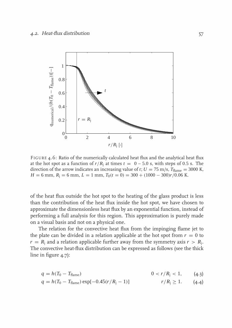
4.2. Heat-flux distribution 57
q numerical/(h
(T0−
T flam
e))
[−]
r/Rj [-]
r = Rj
t
00
0.2
0.4
0.6
0.8
1
2 4 6 8 10
FIGURE 4.6: Ratio of the numerically calculated heat flux and the analytical heat fluxat the hot spot as a function of r/Rj at times t = 0 – 5.0 s, with steps of 0.5 s. Thedirection of the arrow indicates an increasing value of t ; U = 75 m/s, Tflame = 3000 K,H = 6 mm, Rj = 6 mm, L = 1 mm, T0(t = 0) = 300 + (1000 − 300)r/0.06 K.
of the heat flux outside the hot spot to the heating of the glass product is less
than the contribution of the heat flux inside the hot spot, we have chosen to
approximate the dimensionless heat flux by an exponential function, instead of
performing a full analysis for this region. This approximation is purely madeon a visual basis and not on a physical one.
The relation for the convective heat flux from the impinging flame jet to
the plate can be divided in a relation applicable at the hot spot from r = 0 to
r = Rj and a relation applicable further away from the symmetry axis r > Rj.
The convective heat-flux distribution can be expressed as follows (see the thickline in figure 4.7):
q = h(T0 − Tflame) 0 < r/Rj < 1, (4.3)
q = h(T0 − Tflame) exp[−0.45(r/Rj − 1)] r/Rj ≥ 1. (4.4)
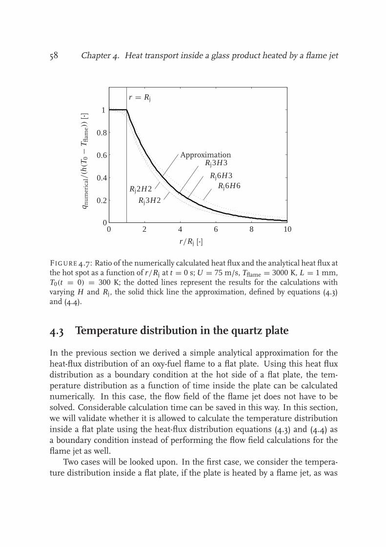
58 Chapter 4. Heat transport inside a glass product heated by a flame jet
q numerical/(h
(T0−
T flam
e))[-]
r/Rj [-]
r = Rj
Rj3H3
Rj6H3Rj6H6Rj2H2
Rj3H2
Approximation
00
0.2
0.4
0.6
0.8
1
2 4 6 8 10
FIGURE 4.7: Ratio of the numerically calculated heat flux and the analytical heat flux atthe hot spot as a function of r/Rj at t = 0 s; U = 75 m/s, Tflame = 3000 K, L = 1 mm,T0(t = 0) = 300 K; the dotted lines represent the results for the calculations withvarying H and Rj, the solid thick line the approximation, defined by equations (4.3)and (4.4).
4.3 Temperature distribution in the quartz plate
In the previous section we derived a simple analytical approximation for the
heat-flux distribution of an oxy-fuel flame to a flat plate. Using this heat flux
distribution as a boundary condition at the hot side of a flat plate, the tem-
perature distribution as a function of time inside the plate can be calculatednumerically. In this case, the flow field of the flame jet does not have to be
solved. Considerable calculation time can be saved in this way. In this section,
we will validate whether it is allowed to calculate the temperature distribution
inside a flat plate using the heat-flux distribution equations (4.3) and (4.4) as
a boundary condition instead of performing the flow field calculations for theflame jet as well.
Two cases will be looked upon. In the first case, we consider the tempera-
ture distribution inside a flat plate, if the plate is heated by a flame jet, as was
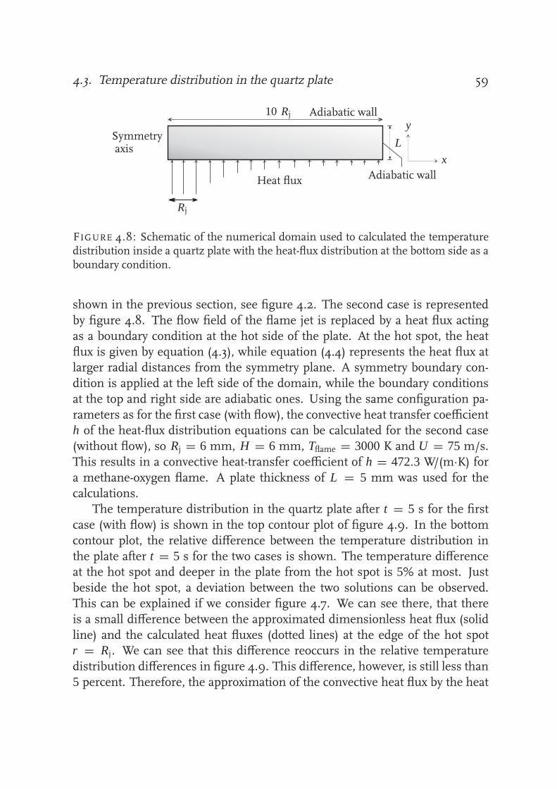
4.3. Temperature distribution in the quartz plate 59
Symmetryaxis
Adiabatic wall
Adiabatic wall
Heat flux
Rj
Rj
10
L
x
y
FIGURE 4.8: Schematic of the numerical domain used to calculated the temperaturedistribution inside a quartz plate with the heat-flux distribution at the bottom side as aboundary condition.
shown in the previous section, see figure 4.2. The second case is represented
by figure 4.8. The flow field of the flame jet is replaced by a heat flux acting
as a boundary condition at the hot side of the plate. At the hot spot, the heat
flux is given by equation (4.3), while equation (4.4) represents the heat flux atlarger radial distances from the symmetry plane. A symmetry boundary con-
dition is applied at the left side of the domain, while the boundary conditions
at the top and right side are adiabatic ones. Using the same configuration pa-
rameters as for the first case (with flow), the convective heat transfer coefficienth of the heat-flux distribution equations can be calculated for the second case
(without flow), so Rj = 6 mm, H = 6 mm, Tflame = 3000 K and U = 75 m/s.
This results in a convective heat-transfer coefficient of h = 472.3 W/(m·K) fora methane-oxygen flame. A plate thickness of L = 5 mm was used for the
calculations.The temperature distribution in the quartz plate after t = 5 s for the first
case (with flow) is shown in the top contour plot of figure 4.9. In the bottom
contour plot, the relative difference between the temperature distribution in
the plate after t = 5 s for the two cases is shown. The temperature differenceat the hot spot and deeper in the plate from the hot spot is 5% at most. Just
beside the hot spot, a deviation between the two solutions can be observed.
This can be explained if we consider figure 4.7. We can see there, that there
is a small difference between the approximated dimensionless heat flux (solid
line) and the calculated heat fluxes (dotted lines) at the edge of the hot spotr = Rj. We can see that this difference reoccurs in the relative temperature
distribution differences in figure 4.9. This difference, however, is still less than
5 percent. Therefore, the approximation of the convective heat flux by the heat
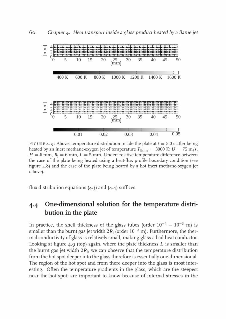
60 Chapter 4. Heat transport inside a glass product heated by a flame jet
[mm]
[mm]
[mm]
[mm]
2
2
4
4
0
0
0
0
5
5
10
10
15
15
20
20
25
25
30
30
35
35
40
40
45
45
50
50
400 K 600 K 800 K 1000 K 1200 K 1400 K 1600 K
0.01 0.02 0.03 0.04 0.05
FIGURE 4.9: Above: temperature distribution inside the plate at t = 5.0 s after beingheated by an inert methane-oxygen jet of temperature Tflame = 3000 K; U = 75 m/s,H = 6 mm, Rj = 6 mm, L = 5 mm. Under: relative temperature difference betweenthe case of the plate being heated using a heat-flux profile boundary condition (seefigure 4.8) and the case of the plate being heated by a hot inert methane-oxygen jet(above).
flux distribution equations (4.3) and (4.4) suffices.
4.4 One-dimensional solution for the temperature distri-
bution in the plate
In practice, the shell thickness of the glass tubes (order 10−4 − 10−3 m) issmaller than the burnt gas jet width 2Rj (order 10−3 m). Furthermore, the ther-
mal conductivity of glass is relatively small, making glass a bad heat conductor.
Looking at figure 4.9 (top) again, where the plate thickness L is smaller than
the burnt gas jet width 2Rj, we can observe that the temperature distribution
from the hot spot deeper into the glass therefore is essentially one-dimensional.The region of the hot spot and from there deeper into the glass is most inter-
esting. Often the temperature gradients in the glass, which are the steepest
near the hot spot, are important to know because of internal stresses in the
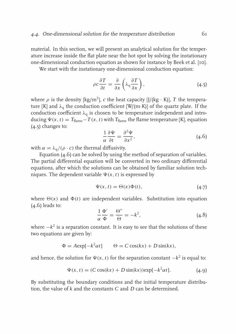
4.4. One-dimensional solution for the temperature distribution 61
material. In this section, we will present an analytical solution for the temper-
ature increase inside the flat plate near the hot spot by solving the instationaryone-dimensional conduction equation as shown for instance by Beek et al. [10].
We start with the instationary one-dimensional conduction equation:
ρc∂T
∂ t= ∂
∂x
(
λq∂T
∂x
)
, (4.5)
where ρ is the density [kg/m3], c the heat capacity [J/(kg · K)], T the tempera-
ture [K] and λq the conduction coefficient [W/(m·K)] of the quartz plate. If theconduction coefficient λq is chosen to be temperature independent and intro-
ducing9(x, t) = Tflame−T (x, t)with Tflame the flame temperature [K], equation
(4.5) changes to:1
α
∂9
∂ t= ∂29
∂x2, (4.6)
with α = λq/(ρ · c) the thermal diffusivity.
Equation (4.6) can be solved by using the method of separation of variables.The partial differential equation will be converted in two ordinary differential
equations, after which the solutions can be obtained by familiar solution tech-
niques. The dependent variable 9(x, t) is expressed by
9(x, t) = 2(x)8(t), (4.7)
where 2(x) and 8(t) are independent variables. Substitution into equation
(4.6) leads to:1
α
8′
8= 2′′
2= −k2, (4.8)
where −k2 is a separation constant. It is easy to see that the solutions of these
two equations are given by:
8 = Aexp[−k2αt] 2 = C cos(kx) + D sin(kx),
and hence, the solution for 9(x, t) for the separation constant −k2 is equal to:
9(x, t) = (C cos(kx) + D sin(kx))exp[−k2αt]. (4.9)
By substituting the boundary conditions and the initial temperature distribu-
tion, the value of k and the constants C and D can be determined.

62 Chapter 4. Heat transport inside a glass product heated by a flame jet
Adiabatic wall
Heat flux
L
x
y
FIGURE 4.10: Schematic overview of the analytical model used to solve the instation-ary conduction equation.
Figure 4.10 represents the boundary conditions for the heating of the hotspot of the plate. Heating the hot spot by the oxy-fuel flame is visualized by the
heat flux q at x = 0. At the cold side of the plate, x = L , an adiabatic boundary
condition is applied so no heat is exchanged with the surroundings. At time
t = 0, the plate has a uniform temperature of T = 300 K.The heat flux at the hot side of the plate can be expressed as follows:
q = h(T (0, t) − Tflame) = λg
∂Tg
∂x, (4.10)
where h is the convective heat-transfer coefficient [W/(m2K)] given by equa-
tion (4.2) and where the subscript g refers to the parameters of the gas. Since
λg∂Tg/∂x = λq∂Tq/∂x must hold at x = 0 at all times if radiative heat losses atx = 0 are not taken into account, the boundary conditions can be expressed as
follows:
x = 0 : ∂9
∂x= h
λq9(0, t), (4.11)
x = L : ∂9
∂x= 0. (4.12)
The value of k in equation (4.9) can be solved by implementing equation
(4.9) in the boundary condition equations (4.11) and (4.12). This results in:
kL tan(kL) = h
λqL . (4.13)

4.4. One-dimensional solution for the temperature distribution 63
Since oxy-fuel flames have very high heat-transfer rates, hL/λq ≫ 1. Conse-
quently, the solution for kn can be approximated by
kn = nπ
2L
(
1 − λq
hL
)
, for n = 1, 3, 5 · · · (4.14)
The equation for the temperature in the quartz plate (4.9) can now berewritten as follows:
9(x, t) =∞∑
n=1
Cn cos(kn(L − x))exp[−k2nαt], (4.15)
where the only unknown is Cn . These parameters can be calculated using
9(x, t) = Tflame − T (x, t) at time t = 0, so
9(x, 0) = Tflame − T (x, 0) = g(x), (4.16)
where g(x) = 2700 K for an oxy-fuel flame with a flame temperature of Tflame =3000 K. Subsequently, equation (4.15) is applied at time t = 0, so
9(x, 0) = g(x) =∞∑
n=1
Cn cos(knz), (4.17)
with z = L −x . Multiplying both sides by cos(kmz) and integrating with respect
to z from z = 0 to z = L , Cm can be found:
Cm = 2 sin(km L)g(x)
sin(km L) cos(km L) + km L, for m = 1, 3, 5 · · · (4.18)
A validation of the one-dimensional analytical solution equations (4.15) and
(4.18) is shown in figure 4.11. In the left picture, the heating at the hot side of
the plate is represented by the solid line. The heating at the cold side is rep-resented by the solid line in the right picture. Numerically, the heating curves
are calculated as well. For the case that the plate is heated by an inert flame jet
(with flow), see figure 4.2, the results are plotted with a dashed line. For the
case that the heat flux of the flame jet is represented by the heat-flux distribu-
tion equations (4.3) and (4.4) (without flow), see figure 4.8, the solutions areplotted using a dotted line. A small offset can be observed for the numerical
solution solution at the hot side of the plate compared to the other two solu-
tions. Otherwise, the solutions are quite similar. For the heating at the cold

64 Chapter 4. Heat transport inside a glass product heated by a flame jetTem
perature
[K]
Time [s]
1000
1500
2000
00 2 4 6 8 10
500 Tem
perature
[K]
Time [s]0 2 4 6 8 10
300
350
400
450
500
550
600
650
FIGURE 4.11: Temperature increase at the hot spot at the hot side of the plate(left) and the cold side of the plate (right) as a function of time; U = 75 m/s,Tflame = 3000 K, H = 6 mm, Rj = 6 mm, L = 5 mm, h = 472.3 W/(m·K).The solid line represents the one-dimensional analytical solution, the dotted linethe axisymmetrical numerical solution with the heat-flux boundary condition (seefigure 4.8) and the dashed line the axisymmetrical numerical solution with flow(see figure 4.2).
side of the plate, the same can be said. Therefore, using the analytical solutionof the instationary one-dimensional conduction equation with the solutions of
the heat flux as a boundary condition, we have a powerful and simple tool at
our disposal to calculate the temperature distribution in a plate heated by an
oxy-fuel flame jet, if we do not take radiative heat losses into account.
4.5 Experimental validation
Various reports on experimental flame-impingement heat-transfer investiga-tions can be found in literature [15, 44, 57]. None of these studies, however,
attempted to generalize the results for later use [66]. Recently, several heat-flux
measurements have been performed on impinging flame jets [19, 20, 38, 39,
67]. Premixed mixtures of fuel and air were used for the experiments. The
heat-transfer characteristics of premixed air-fuel mixtures, however, differ sig-nificantly from mixtures where pure oxygen is used as an oxidizer. For air-fuel
flames, the peak heat flux is shifted away from the stagnation point, whereas
the peak heat flux for oxy-fuel flames occurs at the stagnation point [8].

4.5. Experimental validation 65
In thementioned literature reports, mainly calorimeters and heat-flux trans-
ducers are used for the heat-flux measurements. For the calorimeter measure-ments, data were only reported for steady-state conditions. Furthermore, local
heat-transfer data can not be extracted, since it is an integral measurement
method. Local data were obtained using heat-flux transducers attached to the
center of the heated side of the plate. Although such a transducer is very thin,resulting in a negligible influence on the flow, the impingement surface is rela-
tively large (typically 4×4 mm), so there is a difference in conductivity between
the transducer and the plate which is not trivial.
In this section, we present temperature measurements at a plate heated by
an oxy-fuel flame which are based on a thermometry technique. From the tem-perature increase of the plate, the corresponding heat fluxes can be extracted.
Since measurements at the heated side of the plate are very hard due to the
high temperature and velocity of oxy-fuel flames, experimental validations of
the temperature have been performed on the other side of the plate. The quartz
plate used for these experiments was heated by a methane-oxygen as well as ahydrogen-oxygen flame.
As we have seen in the previous sections, the temperature increase of a
plate heated by an oxy-fuel flame can also be calculated analytically. The heat
fluxes we presented which serve as a boundary condition, however, only ac-count for the convective part of the heat transfer. Cremers [17] has shown that
the total heat flux, where the effect of TCHR is incorporated, can be calculated
by multiplying the convective heat-transfer coefficient h by a so-called TCHR
factor. This TCHR factor mostly depends on the fuel of the flame, the temper-
ature of the plate and the strain rate. To validate the total heat flux obtained inthis way, the results of the calculated temperature increase will be compared
with the measured temperature increase.
4.5.1 Single-point temperature measurements
The measurement technique used for the measurements is based on phos-
phor thermometry. For a more detailed description of this technique, we refer
the reader to Omrane [48], while a review article about phosphor thermometry
written by Allison [1] is useful as well. In recent years this phosphorescencetechnique has been developed for remote measurements of surface temper-
ature. It is based on measuring temperatures by seeding the material with
a temperature-sensitive thermographic phosphor. Thermographic phosphors
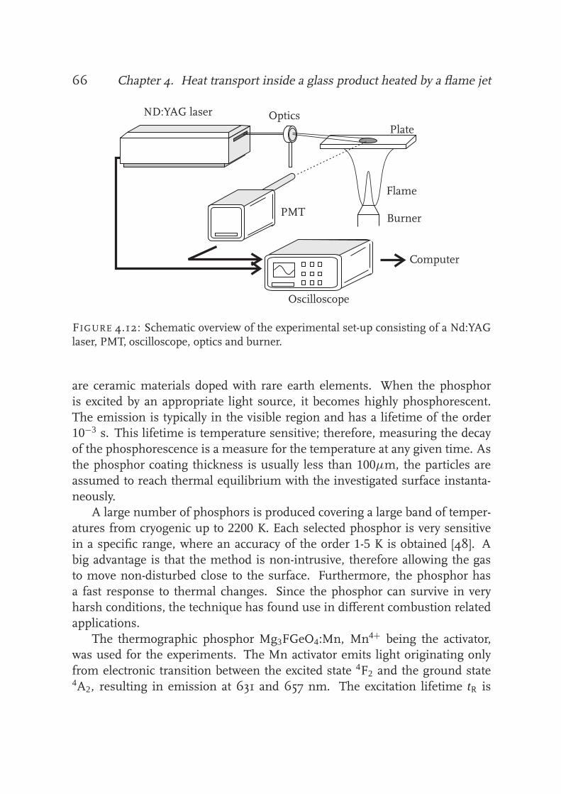
66 Chapter 4. Heat transport inside a glass product heated by a flame jet
ND:YAG laser OpticsPlate
Flame
Burner
Computer
Oscilloscope
PMT
FIGURE 4.12: Schematic overview of the experimental set-up consisting of a Nd:YAGlaser, PMT, oscilloscope, optics and burner.
are ceramic materials doped with rare earth elements. When the phosphor
is excited by an appropriate light source, it becomes highly phosphorescent.
The emission is typically in the visible region and has a lifetime of the order10−3 s. This lifetime is temperature sensitive; therefore, measuring the decay
of the phosphorescence is a measure for the temperature at any given time. As
the phosphor coating thickness is usually less than 100µm, the particles are
assumed to reach thermal equilibrium with the investigated surface instanta-
neously.A large number of phosphors is produced covering a large band of temper-
atures from cryogenic up to 2200 K. Each selected phosphor is very sensitive
in a specific range, where an accuracy of the order 1-5 K is obtained [48]. A
big advantage is that the method is non-intrusive, therefore allowing the gasto move non-disturbed close to the surface. Furthermore, the phosphor has
a fast response to thermal changes. Since the phosphor can survive in very
harsh conditions, the technique has found use in different combustion related
applications.
The thermographic phosphor Mg3FGeO4:Mn, Mn4+ being the activator,was used for the experiments. The Mn activator emits light originating only
from electronic transition between the excited state 4F2 and the ground state4A2, resulting in emission at 631 and 657 nm. The excitation lifetime tR is

4.5. Experimental validation 67
TABLE 4.1: Values of different parameters of methane-oxygen and hydrogen-oxygenflames. The values are chosen at a temperature of 1500 K, with exception of the densityof the burnt gases ρb and the expansion factor τ .
ρb λ cp µ τ TCHR
[kg/(m3· s)] [W/(m·K)] [J/(kg · K)] [kg/(m · s)] [-] [-]
CH4-O2 0.083 0.16 2.0 · 103 5.6 ·10−5 12.6 2.0H2-O2 0.059 0.30 2.5 · 103 5.6 ·10−5 8.3 2.0
strongly temperature dependent as reported by Omrane [48]. In figure 4.12,a schematic of the experimental set-up is shown. The phosphor was coated
to the surface using the non-fluorescent binder HPC found to be suitable for
harsh conditions [2]. Excitation of the phosphor was conducted using the third
harmonic at 355 nm of a Nd:YAG laser with a pulse duration of 8 ns and a
repetition rate of 10 Hz. A laser intensity of 8 mJ was used to obtain phospho-rescence. The laser light was focused on the top side of a quartz plate directly
above the hot spot, where the radius of the hot spot was equal to Rj, which is
the radius of the burnt gas flow tube. The dimensions of the quartz plate were
equal to 100 × 100 × 5 mm. The part of the top side of the plate directly abovethe hot spot was coated with the phosphor. The subsequent emission was col-
lected by a photomultiplier tube (PMT). A 3 GHz oscilloscope, triggered by the
laser, was used to digitize the signal from the PMT. The measured emission
decay was fitted to the theoretical model I = I0 · exp[−t/tR] and compared to
a calibration curve. Both a methane-oxygen and hydrogen-oxygen flame wereused to heat the quartz plate. The premixed gas mixture was supplied to the
burner using a mixing panel with Mass Flow Controllers (MFCs), which were
set and monitored using an interface to a PC. The burner nozzle diameter was
equal to d = 1.7 mm. Remie [54] has shown that the resulting radius of theburnt gas jet will be equal to Rj = τ 0.5 · d/2, with τ the expansion coefficient.
The different parameters for both flames are shown in table 4.1. Since τ = 12.6for the methane-oxygen flames, Rj = 3.0 mm. For the hydrogen-oxygen flames
with τ = 8.3, Rj = 2.4 mm. The measurements were performed for an un-
burnt gas velocity of 70 m/s and flame tip-to-plate distances of H = 2, 5, 10and 20 mm.
Figure 4.13 shows a typical result of a temperature measurement of the
quartz plate heated by a flame (solid line). For this measurement, a methane-
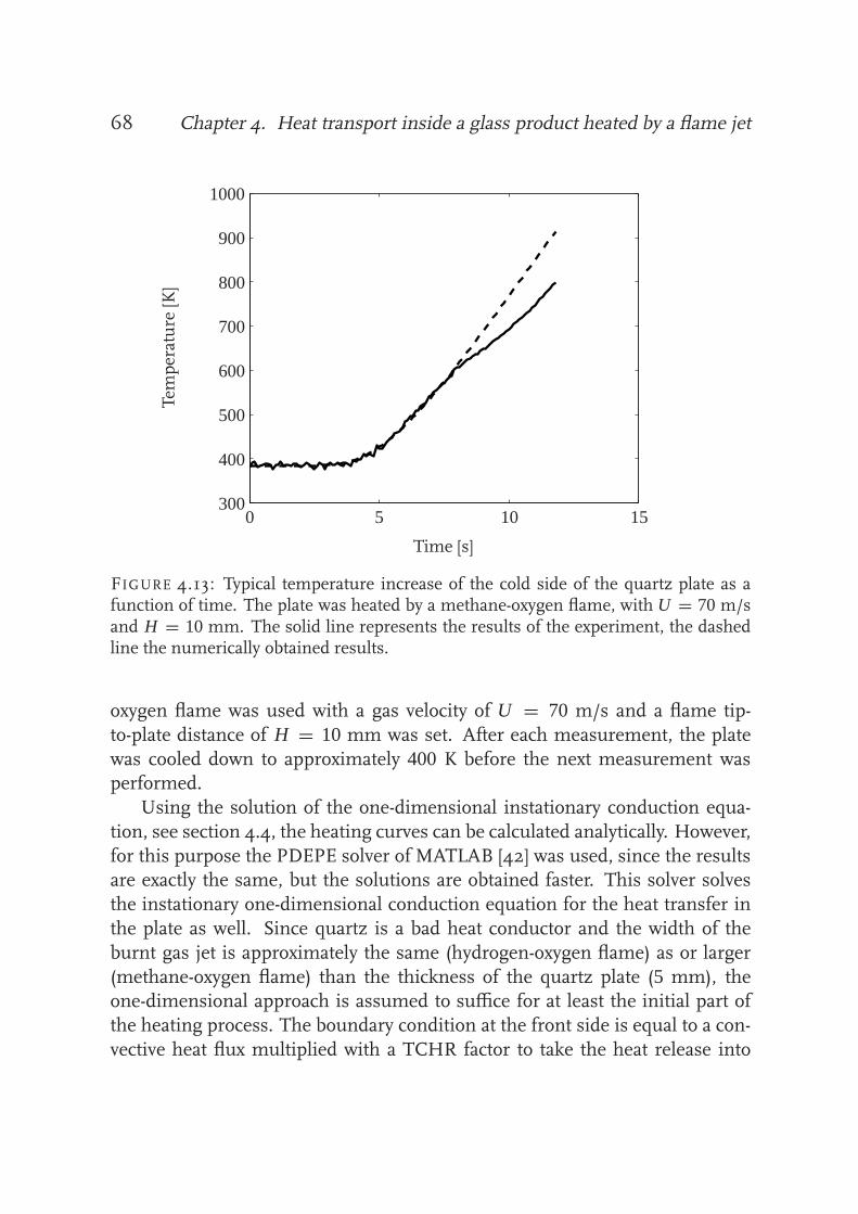
68 Chapter 4. Heat transport inside a glass product heated by a flame jet
Tem
perature
[K]
Time [s]
300
400
500
600
700
800
900
1000
0 5 10 15
FIGURE 4.13: Typical temperature increase of the cold side of the quartz plate as afunction of time. The plate was heated by a methane-oxygen flame, with U = 70 m/sand H = 10 mm. The solid line represents the results of the experiment, the dashedline the numerically obtained results.
oxygen flame was used with a gas velocity of U = 70 m/s and a flame tip-
to-plate distance of H = 10 mm was set. After each measurement, the plate
was cooled down to approximately 400 K before the next measurement wasperformed.
Using the solution of the one-dimensional instationary conduction equa-
tion, see section 4.4, the heating curves can be calculated analytically. However,
for this purpose the PDEPE solver of MATLAB [42] was used, since the resultsare exactly the same, but the solutions are obtained faster. This solver solves
the instationary one-dimensional conduction equation for the heat transfer in
the plate as well. Since quartz is a bad heat conductor and the width of the
burnt gas jet is approximately the same (hydrogen-oxygen flame) as or larger
(methane-oxygen flame) than the thickness of the quartz plate (5 mm), theone-dimensional approach is assumed to suffice for at least the initial part of
the heating process. The boundary condition at the front side is equal to a con-
vective heat flux multiplied with a TCHR factor to take the heat release into

4.5. Experimental validation 69
account which is released after the recombination of radicals at the cold plate
surface. A value of 2.0 is chosen for the TCHR factor for both flames, selectedat a temperature of T = 1500 K [17]. The values of the gas parameters are
also chosen at a temperature of T = 1500 K, as was done in the previous sec-
tions, see table 4.1. An adiabatic boundary condition was set at the cold side
of the plate. Since only the initial part of the heating process is considered,radiation does not have to be taken into account. Like in the previous sections,
the parameters of the quartz plate are chosen to be equal to ρ = 2250 kg/m3,
cp = 780 J/(kg·K) and λ = 0.75 · 1.4 W/(m·K) [12].To be able to compare the numerically obtained heating curves with the
experimentally obtained heating curves, a non-linear least squares fitting pro-cedure is used. A good fitting requires that as few as possible parameters are
varied. In this case, the most obvious choice is to vary the total heat transfer
coefficient h, the initial temperature and the point of time where the flame is
ignited. A typical result of such a fit is shown in figure 4.13, where the numer-
ical results of the heating of the cold side of the quartz plate are representedby the dashed line. Initially, a good agreement can be observed. After about 8seconds, a deviation can be observed. At that time, the hot side of the plate got
very hot resulting in a strong Planck radiation visible as a red glow. Therefore,
thermal radiation leading to a too high DC level on the PMT could have inter-fered with the measurements, resulting in a non-linear response and thus too
low temperatures in the evaluation. To minimize this affect, only a fit for the
initial part of the heating was performed.
Using the fitting procedure, for every measurement a convective heat flux
can be determined. It is also possible to calculate an analytical convective heatflux for each measured situation using equations (3.19) and (3.23). Let us now
compare the analytically and experimentally obtained heat fluxes using a heat-
flux figure similar to figure 3.10.
Figure 4.14 shows the comparisons between the analytically obtained con-vective heat fluxes and the experimentally obtained convective heat fluxes for
the methane-oxygen flame (left) and the hydrogen-oxygen flame (right). The
solid lines represent the analytical solutions for the heat flux, the circles the
experimentally determined heat fluxes. The horizontal error bars are obtained
by taking into account the inaccuracy of the manually set flame tip-to-plate dis-tance H (0.2 mm, which is approximately the flame thickness). The vertical
error bars are obtained by using a 95 % confidence interval (2σ error) of the
variance of the heat-transfer coefficient h. The figures show a good agreement
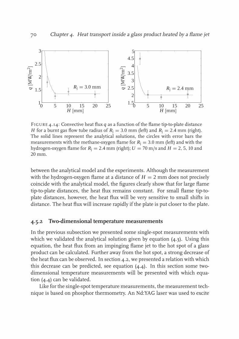
70 Chapter 4. Heat transport inside a glass product heated by a flame jetq[M
W/m
2 ]
H [mm]
Rj = 3.0 mm
1
1.5
2
2.5
3
0 5 10 15 20 25
q[M
W/m
2 ]
H [mm]
Rj = 2.4 mm
1.5
2
2.5
3
3.5
4
4.5
0
5
5 10 15 20 25
FIGURE 4.14: Convective heat flux q as a function of the flame tip-to-plate distanceH for a burnt gas flow tube radius of Rj = 3.0 mm (left) and Rj = 2.4 mm (right).The solid lines represent the analytical solutions, the circles with error bars themeasurements with the methane-oxygen flame for Rj = 3.0 mm (left) and with thehydrogen-oxygen flame for Rj = 2.4 mm (right); U = 70 m/s and H = 2, 5, 10 and20 mm.
between the analytical model and the experiments. Although the measurement
with the hydrogen-oxygen flame at a distance of H = 2 mm does not precisely
coincide with the analytical model, the figures clearly show that for large flame
tip-to-plate distances, the heat flux remains constant. For small flame tip-to-plate distances, however, the heat flux will be very sensitive to small shifts in
distance. The heat flux will increase rapidly if the plate is put closer to the plate.
4.5.2 Two-dimensional temperature measurements
In the previous subsection we presented some single-spot measurements with
which we validated the analytical solution given by equation (4.3). Using thisequation, the heat flux from an impinging flame jet to the hot spot of a glass
product can be calculated. Further away from the hot spot, a strong decrease of
the heat flux can be observed. In section 4.2, we presented a relation with which
this decrease can be predicted, see equation (4.4). In this section some two-
dimensional temperature measurements will be presented with which equa-tion (4.4) can be validated.
Like for the single-spot temperaturemeasurements, themeasurement tech-
nique is based on phosphor thermometry. An Nd:YAG laser was used to excite

4.5. Experimental validation 71replacements
ND:YAG laserOptics
Plate
Flame
Burner
Mirror
Stereoscope
ICCD
FIGURE 4.15: Schematic overview of the experimental set-up consisting of a Nd:YAGlaser, ICCD, stereoscope, optics, mirror and burner.
the phosphor. The lifetime of the phosphorescence decay and the emission line
intensities are temperature sensitive. For the single-spot temperature measure-ments, the lifetime of the decay of the phosphorescence is extracted, in order to
obtain the plate temperature. For the two-dimensional temperature measure-
ments, however, a spectral method was used instead of a temporal method.
Now the intensity of two different emission lines is imaged. Since the ratio ofthese two apparent peak intensities of the phosphor is only dependent on tem-
perature, this technique is suitable for measuring the temperature distribution
of the cold site of the quartz plate heated by an impinging flame jet. Spectral
profiles of different phosphors are reported by Omrane [48], while a more de-
tailed analysis of the measurement method can be found in refs. [1, 48, 47, 59].Figure 4.15 shows a schematic overview of the experimental set-up. For
these two-dimensional temperature measurements, the thermographic phos-
phor YAG:Dy was used. Excitation of the phosphor was conducted using the
third harmonic at 355 nm of an Nd:YAG laser with a pulse duration of 8 ns anda repetition rate of 10 Hz. A laser intensity of 130 mJ was used to obtain phos-
phorescence. The laser light was directed to the top side of the quartz plate.
To split the measured image into two identical images, a stereoscopic device
with an interference filter of 458 nm and an interference filter of 493 nm was
adapted to the objective of an Intensified Charge-Coupled Device (ICCD) cam-era. For the experiment, the same quartz plate and burner were used as for
the single-spot temperature measurements. Measurements were performed
for a methane-oxygen as well as a hydrogen-oxygen flame with an unburnt gas

72 Chapter 4. Heat transport inside a glass product heated by a flame jet
10
20
30
40
50
60
70
80
90
20 40 60 80
400 K
450 K
500 K
550 K
600 K
650 K
700 K
750 K
20
40
60
80
20 40 60 80
400
500
600
700
FIGURE 4.16: Temperature distribution of the cold site of the plate after 8 secondsvisualized with a grayscaling (left) and isothermal contours (right); the center of thehot spot is indicated by the asterisk in the right figure. The plate was heated by ahydrogen-oxygen flame; U = 70 m/s, Rj = 2.4 mm, H = 20 mm.
velocity of 70 m/s and different flame tip-to-plate distances H .
Figure 4.16 shows a typical result of a temperature distribution measure-
ment of the top side of the plate after t = 8 s. The plate was heated by ahydrogen-oxygen flame with U = 70 m/s and H = 20 mm. After each mea-
surement, the plate was cooled down to approximately 400 K before the next
measurement was performed. In the right figure, the center of the hot spot is
visualized by the asterisk. Its position was determined as the center of ’mass’
of the temperature distribution.As was explained in the previous subsection, the heating curves of the hot
spot at the cold side of the plate were determined using the PDEPE solver of
MATLAB. Analogously, a non-linear least squares fitting procedure was used
to compare the numerically obtained heating curves of the hot spot at the coldside of the plate with the experimentally obtained heating curves of the hot
spot at the cold side of the plate. For every measurement, a convective heat flux
can be determined experimentally as well as analytically. Figure 4.17 shows the
comparison between the analytically and the experimentally obtained convec-
tive heat fluxes for the methane-oxygen flame (left) and the hydrogen-oxygenflame (right). The analytical solutions are represented by the solid lines, the
circles represent the experimentally determined heat fluxes. The error bars are
obtained as explained in the previous subsection. As was shown in the pre-

4.5. Experimental validation 73q[M
W/m
2]
H [mm]
Rj = 3.0 mm
1
1.5
2
2.5
3
0 5 10 15 20 25
q[M
W/m
2]
H [mm]
Rj = 2.4 mm
1.5
2
2.5
3
3.5
4
4.5
0 5 10 15 20 25
FIGURE 4.17: Convective heat flux q as a function of the flame tip-to-plate distanceH for a burnt gas flow tube radius of Rj = 3.0 mm (left) and Rj = 2.4 mm (right).The solid lines represent the analytical solutions, the circles with error bars themeasurements with the methane-oxygen flame for Rj = 3.0 mm (left) and with thehydrogen-oxygen flame for Rj = 2.4 mm (right); U = 70 m/s and H = 1, 2, 10 and20 mm (left) and H = 1, 2, 5, 10 and 20 mm (right).
vious subsection, for large flame tip-to-plate distances the convective heat flux
is constant, while the convective heat flux at small flame tip-to-plate distancesbecomes very sensitive for small shifts in distance H .
Using the results of figure 4.16, a scatter plot of the temperature at the top
side of the plate as a function of the radial distance to the center of the hot spot
can be obtained. Such a scatter plot is shown in figure 4.18. A methane-oxygen
flame was used to heat the plate, with U = 70 m/s and H = 10 mm. The bigdots represent the averaged measurement results. To obtain such a tempera-
ture distribution curve numerically, the same calculations were performed as
explained in section 4.3. A plate with thickness L = 5 mm was heated using
the heat-flux boundary equations (4.3) and (4.4), see figure 4.8. For the velocityU and the flame tip-to-plate distance H , the same values were used as in the
experimental configuration. In figure 4.18, the numerical result is represented
by the solid line.
To validate the heat-flux distribution relation given by equation (4.4), figure
4.18 shows the half maximum - half width values of the numerically and exper-imentally obtained temperature distribution. For this situation, the difference
is only 1.5 mm and therefore equation (4.4) seems to hold. Table 4.2 shows the
results of all the measurements.

74 Chapter 4. Heat transport inside a glass product heated by a flame jet
Tem
perature
[K]
Radial distance [mm]
300
400
500
600
700
800
0 10 20 30 40 50
FIGURE 4.18: Typical temperature distribution of the cold side of the quartz plat asa function of the radial distance to the center of the hot spot at t = 8 s. The platewas heated by a methane-oxygen flame, with U = 70 m/s and H = 10 mm. Thesmall dots represent the measurement results, the big dots the averaged measurementresults and the solid line the numerically obtained results. The thin solid lines showthe difference in the numerically and experimentally obtained half maximum - halfwidth values.
TABLE 4.2: Values of the half maximum - half width value differences between theexperiments and the numerical calculations.
H = H = H = H = H =1 mm 2 mm 5 mm 10 mm 20 mm
CH4-O2 1.0 mm 2.0 mm - 1.5 mm 2.0 mm
H2-O2 4.0 mm 1.0 mm 1.0 mm 0.5 mm 2.0 mm
4.6. Conclusions 75
4.6 Conclusions
In the glass heating process, it is important to know what the temperature dis-
tribution inside the product is, considering internal thermal stresses. There-
fore, the heat-flux distribution of an impinging flame jet to a glass product is
essential. In chapter 3 a relation was already presented for the convective heatflux of an impinging flame jet to the hot spot of the product. In this chapter
an additional convective heat-flux relation is introduced, applicable for larger
radial distances from the hot spot. At the edge of the hot spot at r = Rj, the two
heat-flux relations are linked to each other.
An advantage of having the two relations describing the convective heat-fluxdistribution at our disposal, is that in this case the temperature distribution in-
side a glass product can be calculated with the heat-flux relations as a boundary
condition, instead of performing flow calculations of the flame jet as well to
calculate the temperature distribution. Comparison between these two cases
reveal a relative temperature difference of only 5% at most, occurring aroundthe edge of the hot spot at r = Rj where the two heat-flux relations are linked
to each other.
Since the largest temperature gradients and therefore the highest thermal
stresses can be found from the hot spot deeper into the glass, this region of theproduct is most important. Furthermore, the shell thickness of the glass prod-
uct is smaller than the burnt gas width 2Rj in practice. Considering the fact
that glass is a bad heat conductor, the temperature distribution from the hot
spot deeper into the glass is essentially one-dimensional. A one-dimensional
solution is presented of the instationary conduction equation, with the convec-tive heat-flux relation applicable for the hot spot as a boundary condition. With
this solution a simple and fast tool to calculate the temperature distribution in
the product near the hot spot is available, assuming that the influence of ra-
diative heat losses is negligible. Validation with numerical calculations show agood agreement.
Experimental validations have been performed for the analytical convec-
tive heat-flux relations. For that purpose, phosphor thermometry techniques
have been applied. For the validation of the convective heat-flux relation appli-
cable at the hot spot, single-point temperature measurements have been car-ried out. The results clearly show that the heat flux is constant for large flame
tip-to-plate distances and increases rapidly for shorter distances, which is in
agreement with the analytical heat-flux relations. Two-dimensional tempera-

76 Chapter 4. Heat transport inside a glass product heated by a flame jet
ture measurements, performed to validate the heat-flux relations applicable at
radial distances away from the hot spot, show good agreement as well.

Chapter
5Practical applications
5.1 Introduction
In the previous chapters, the importance of knowing the heat flux from an
impinging flame jet to a glass product with regard to high thermal stressesand overheated hot spots has been indicated. Heat-transfer relations have been
derived analytically and validated both numerically and experimentally by ap-
proximating the process as a small laminar oxy-fuel jet impinging on a product,
which is a common configuration in the lamp-making process. In this chap-ter the acquired knowledge from the previous chapters will be combined and
applied to some problems encountered in practice.
Next to the flame temperature, gas velocity and flame tip-to-plate distance,
the heat flux from an impinging flame jet to a product depends on the choice of
fuel. In the following section, it will be shown step by step how the heat flux ofan impinging flame jet to a glass product can be calculated. Subsequently, a an
example of the heat flux of several flame jets, positioned inline, heating a glass
product is presented. At first the corresponding burner is fed with a hydrogen-
oxygen mixture; it will be shown how the heat flux changes for the case that theburner will be operated with a methane-oxygen mixture. Obviously, changing
the type of fuel will have consequences for the operating conditions. Section
5.4 shows how the exit velocity of the unburnt gases changes, if the pressure
drop over the burner is kept constant while the gas mixture is switched from
hydrogen-oxygen to methane-oxygen. One way of increasing the heat flux, isincreasing the gas velocity. Increasing the gas velocity of course has its limits: at
a certain velocity, the flame will not stabilize on the burner nozzle and will blow
off. This blowoff gradient will be discussed in section 5.5. Finally, quartz vapor
77

78 Chapter 5. Practical applications
Wall jet region
Viscous boundary layer
Stagnation region
Free jet region
Flame jet region
Burner
Impingementsurface
H
Hflame
Htot
URj
Rb
x, u
r, v
FIGURE 5.1: Schematic overview of a stagnation flame impinging on a plane surface.
from the heated product often settles on the burner. This burner fouling is animportant phenomenon since it has a considerable influence on the heat flux
from the flame jet to the product. Essentially, the flame will stabilize differently
on the burner nozzle causing a smaller distance between the flame tip and
the plate and/or a smaller flame jet with a higher gas velocity. How large this
influence is, can be investigated with the earlier derived heat-flux relations andwill be treated in the last section.
5.2 From burner nozzle to product: prediction of the heat
flux
In this section we will summarize how the heat flux from an impinging flame
jet to a glass product can be calculated. Figure 5.1 shows the configuration of
a single flame jet heating a flat plate. As described in chapter 1, four different
regions can be distinguished: a flame jet region, a free jet region, a stagna-
tion region and a wall jet region. In each region different physical phenomenatake place which all have their own time scales. Since these time scales are of
different orders of magnitude, we are able to decouple the regions, treat them
separately and couple them again afterwards.

5.2. From burner nozzle to product: prediction of the heat flux 79
To calculate the heat flux of an impinging flame to the hot spot of a plate
such as represented in figure 5.1, let us first start with the burner. As can beseen in figure 2.5, the burner is usually constructed in such a way, that the
shape of the unburnt oxy-fuel mixture exiting the burner nozzle is close to a
perfect plug flow. Since for oxy-fuel flames the burning velocity of the mixture
sL [m/s] is a lot smaller than the unburnt gas velocity u1 [m/s], only a smalldivergence of the burnt gases after expansion over the flame front takes place.
Consequently, the dip in the velocity profile directly above the flame tip is small
and the resulting flow after expansion is close to a perfect plug flow as well. In
that case, we can use the polynomial given by equation (2.10) to calculate the
velocity of the burnt gases u2 [m/s] and the burnt gas jet radius Rj [m].After rearranging the solution of the polynomial, equation (2.10), the ex-
pansion can be calculated with:
(
Rb
Rj
)2
= 1 −√
(
1 − s2L
u21
)
τ 2 − 2τ + 1
τ 2, (5.1)
with Rb the burner radius [m] and with τ = ρu/ρb [-], ρu being the density ofthe unburnt mixture [kg/m3] and ρb the density of the burnt mixture. Using
the conservation of mass, equation (2.4), combined with the relation describing
the expansion of the gases, equation (5.1), results in the following velocity ratio:
u2
u1= τ
(
1 −√
(
1 − s2L
u21
)
τ 2 − 2τ + 1
τ 2
)
. (5.2)
As can be seen from these two equations, the velocity and the jet width of the
burnt gases in the free jet region can easily be calculated if the unburnt gas
velocity u1, the burning velocity sL and the expansion coefficient τ are known.
For oxy-fuel mixtures where τ ≫ 1 and sL ≪ u1, the solution of the expansion
(5.1) and the velocity ratio (5.2) can even be simplified to:
Rj =√
τ Rb, (5.3)
u2 = u1. (5.4)
Now we have the velocity of the burnt gases and the width of burnt gasjet at our disposal. Together with the temperature of the burnt gases and the
distance between the flame tip and the plate H , these parameters serve as input
parameters to calculate the convective heat flux to the product.

80 Chapter 5. Practical applications
Flame front
α
sL
Hflameu1
Rb
FIGURE 5.2: Schematic overview of the flame front.
In practice, the burner-to-plate distance Htot (see figure 5.1) is a setup pa-
rameter instead of the flame tip-to-plate distance H . Since the flame tip-to-
distance H is an input parameter for the calculation of the convective heat fluxand H = Htot − Hflame, the flame height Hflame needs to be known. Looking at
the schematic overview of the flame front in figure 5.2, where curvature effects
at the edge of the burner nozzle and the flame tip are assumed to be negligible,
the flame height Hflame can be expressed as follows:
Hflame = Rb
tan(arcsin(sL/u1)), (5.5)
and therefore:
H = Htot −Rb
tan(arcsin(sL/u1)). (5.6)
If the flame temperature is known, all the input parameters are known.
Dependent on the configuration, equations (3.13) and (3.14) (single flame jet ormatrix set up of several flame jets) or equations (A.13) and (A.14) (several flame
jets positioned inline) describe the axial velocity profile of the burnt gases in the
stagnation region for r = 0 up to close to r = Rj. Close to r = Rj, due to mixing

5.2. From burner nozzle to product: prediction of the heat flux 81
with the surrounding air, the axial velocity decreases rapidly. If radiative heat
losses of the gases and of the product at the hot side can be neglected whichis especially the case for the initial heating process, conservation of energy in
the boundary layer close to the product in the hot spot region (r = 0 to r = Rj)
implies a balance of convection and conduction. The resulting convective heat
flux can then be expressed as follows:
q0 = λdT
dx
∣
∣
∣
0= λ(T0 − Tflame)
0∫
−H∗exp
[
− 1α
0∫
sudx
]
ds
, (5.7)
with λ the conductivity coefficient [W/(m·K)], T0 the temperature at the hot side
of the plate [K], Tflame the flame temperature, α the thermal diffusivity [m2/s]and u the axial velocity profile [m/s].
For a single flame jet or a matrix set up of several flame jets, the solution
of the axisymmetrical axial velocity profile described by equations (3.13) and
(3.14) can be implemented in equation (5.7) to calculate the convective heat
flux. Dependent on the distance between the flame tip and the product, thevalue of H∗ is equal to the distance between the flame tip and the product H(if H < 5Rj/3) or equal to 5Rj/3 (if H ≥ 5Rj/3). The denominator of equation
(5.7) for this case becomes equal to:
0∫
−H∗
exp
− 1
α
0∫
s
udx
ds =H∗0∫
−xδ/H∗
exp
1
12
Pe2
Prx ′4 +
√
4
18
Pe3
Prx ′3
ds ′+
H∗−xδ/H∗∫
−1
exp
[
−Pr − Pe
(
1
3x ′3 + 1
3
√
2Pr
Pex ′2+
1
9
2Pr
Pex ′ + 1
9
√
2Pr
Pe
3
+ x ′2+
2
3
√
2Pr
Pex ′ − 1
3
2Pr
Pe
)]
ds ′, (5.8)
where Pe = U H∗/α is the Peclet number [-], Pr = ν/α the Prandtl number[-] with ν the kinematic viscosity [m2/s] and xδ = 2
√ν/a the viscous boundary
layer thickness [m] with a = 2U/H the maximum strain rate of the burnt gases
[1/s].

82 Chapter 5. Practical applications
If several flame jets positioned inline are used to heat the glass product,
however, the axial velocity profile described by equations (A.13) and (A.14) needto be implemented in equation (5.7) to calculate the convective heat flux. The
value of H∗ is now equal to H (for H < 2Rj) or equal to 2Rj (for H ≥ 2Rj). In
this case, the denominator of equation (5.7) becomes equal to:
0∫
−H∗
exp
− 1
α
0∫
s
udx
ds =H∗0∫
−xδ/H∗
exp
π2
96
Pe2
Prx ′4 + 1
12
√
Pe3π3
Prx ′3
ds ′+
H∗−xδ/H∗∫
−1
exp
[
−1
2Pr − 2
πPe
(
cos
(
2
3
√
πPr
Pe
)
−
cos
(
−1
3
√
πPr
Pe− πx ′
2
))]
ds ′,
(5.9)
where the viscous boundary layer is given by xδ =√
2ν/a [m] and the maxi-
mum strain rate by a = πU/(2H). For these flame jets, the equations describ-ing the convective heat flux (5.7) and (5.9) can be simplified considerably to (see
appendix A):
q = λ∂T
∂x
∣
∣
∣
0= λ(T0 − Tflame)
1
H∗
√Pe · exp
[
−0.28Pr0.40]
. (5.10)
Cremers [17] has shown that the total heat flux to the hot spot can be calcu-lated by multiplying the convective heat flux by a so-called TCHR factor. Since
especially the burnt gases of oxy-fuel flames contain a lot of free radicals as a
result of dissociation of stable molecules at high temperatures, additional heat
is released as these radicals enter the cold boundary and recombine. The effect
of this Thermochemical Heat Release is taken into account by multiplying theconvective heat flux by the TCHR factor:
qtotal = TCHR × qconvective, (5.11)
with qtotal the total heat flux to the hot spot.

5.3. Application to flame jets positioned inline 83
TABLE 5.1: Values of different parameters of methane-oxygen and hydrogen-oxygenflames. The values of λ, α and Pr are chosen at a temperature of 1500 K.
Tflame sL λ α Pr τ TCHR
[K] [m/s] [W/(m·K)] [m2/s] [-] [-] [-]
CH4-O2 3052 3.06 0.16 9.6 · 10−4 0.7 12.6 2.0H2-O2 3079 9.97 0.30 2.0 · 10−3 0.5 8.3 2.0
5.3 Application to flame jets positioned inline
In practice, higher heat-transfer rates can be obtained if a hydrogen-oxygen
instead of a methane-oxygen flame is used to process glass products. Since
hydrogen-oxygen flames have a higher burning velocity sL thanmethane-oxygen
flames (see table 5.1), higher burnt gas velocities can be achieved and thereforehigher heat fluxes. Furthermore, looking at the values of the conduction coeffi-
cient λ and the thermal diffusivity coefficient α, for the same flame tip-to-plate
distance H and burnt gas velocity U , the ratio of the convective heat flux ob-
tained with a stoichiometric methane-oxygen flame to the convective heat fluxobtained with a stoichiometric hydrogen-oxygen flame is roughly equal to:
qCH4
qH2
= 0.16
0.30
√
2.0 · 10−3
9.6 · 10−4= 0.77, (5.12)
where equation (5.10) has been used.
However, in some cases it can be advantageous to use methane-oxygen in-stead of hydrogen-oxygen for instance because of safety and economical rea-
sons. In this section the approach explained in the previous section to calculate
the heat transfer of an impinging flame jet to a glass product will be applied
to an example of a burner which produces several flame jets positioned inline.Initially, this burner is fed with a premixed stoichiometric mixture of hydrogen
and pure oxygen. Subsequently, the obtained heat flux will be compared with
the heat flux which is obtained if the burner is fed with a premixed stoichio-
metric methane-oxygen mixture.
We consider the following example. A schematic overview of a glass prod-uct heated by several flame jets positioned inline is represented in figure 5.3.
Since the radius of the glass tube is relatively large compared to the shell thick-
ness, the tube can be approximated by a flat glass plate. Furthermore, the flame

84 Chapter 5. Practical applications
Rj
Rb
HHflameHtot
FIGURE 5.3: Schematic overview of a glass product heated by a burner producingseveral flame jets positioned inline.
jets are positioned close enough to each other, to obtain a two-dimensional con-
figuration and therefore to be able to use equation (5.10) to calculate the con-vective heat flux. An unburnt gas mixture of hydrogen and oxygen is fed to
the burner. The exit diameters of this burner are equal to Rb = 1.0 mm. The
unburnt gas velocity of the mixture is equal to u1 = 40 m/s, while the burner-
to-target distance is set to Htot = 20 mm. The tube is at ambient temperature,
T0 = 300 K. With these configuration data in combination with the gas param-eters of table 5.1, the heat flux of these hydrogen-oxygen flames to the glass
product can be calculated.
Using equations (5.1) and (5.2), the burnt gas jet radius and burnt gas ve-
locity can be calculated:
Rj = 2.6 mm,
u2 = U = 49 m/s.
After applying equation (5.5), the resulting flame height is found to be equal to
Hflame = 3.9 mm and therefore the flame tip-to-plate distance is equal to:
H = Htot − Hflame = 16.1 mm.

5.3. Application to flame jets positioned inline 85
q total[M
W/m
2]
H [mm]
2.5
3
3.5
4
4.5
5
5.5
6
6.5
0 5 10 15 20 25
FIGURE 5.4: Total heat flux qtotal as a function of flame tip-to-target distance H fora burner fed with a hydrogen-oxygen mixture producing flame jets positioned inlinewith Rj = 2.6 mm and U = 49 m/s. The circle represents the calculated configuration(see text), with Htot = 20 mm.
Now every parameter is known to calculate the convective heat flux given by
equation (5.10):
qconvective = 1.46 MW/m2,
and therefore:
qtotal = TCHR × qconvective = 2.9 MW/m2.
Figure 5.4 shows the total heat flux qtotal as a function of the flame tip-to-target distance H for the configuration under consideration. The circle rep-
resents the calculated heat flux for Htot = 20 mm. As can be seen from the
figure, small shifts in distance between the burner and the product do not al-
ter the heat flux from the impinging flames. Considering the stability of the
heating process and the reproducibility of the products, this is advantageous.In the foregoing, we calculated the heat flux from the hydrogen-oxygen
flames to the product by beginning with the burner and via calculating the
burnt gas flow width 2Rj, burnt gas velocity u2 = U , flame height Hflame and

86 Chapter 5. Practical applications
flame tip-to-target distance H , concluding with the heat flux to the product
q. Replacing the hydrogen by methane will have an increase of the burnt gasjet width 2Rj as a consequence, since the expansion coefficient τ of methane-
oxygen is larger than of hydrogen-oxygen, see table 5.1. Using equation (5.1) the
burnt gas jet radius for this case becomes equal to:
Rj = 3.5 mm.
Consequently, the flame height and the burnt gas velocity will, using equations
(5.5) and (5.2), be equal to:
Hflame = 13.0 mm,
u2 = 41 m/s,
and therefore, using equations (5.6) and (5.11):
H = 7.0 mm,
qtotal = 1.7 MW/m2.
The circle marked ’a’ in figure 5.5 represents the calculated situation. Plac-
ing the tube closer to the flame front to H = 2.4 mm or Htot = 15.4 mm re-sults in a heat flux of qtotal = 2.9 M/W2 (circle ’b’). For this situation, however,small shifts in distance result in large alterations of the heat flux. Therefore,
although the same heat flux is obtained as for the case where the tube is heated
with hydrogen-oxygen flames, this configuration is not preferable. In order to
obtain the same heat flux while keeping the heating process stable to maintaina good reproducibility of the products, it is preferred to have a critical distance
equal to H∗ > 2Rj. Using figure 3.10, it can be seen that decreasing the burner
hole radii resulting in smaller burnt gas jet radii Rj, and increasing the gas
velocity will result in a higher heat flux.
5.4 Pressure drop over the burner: a comparison
As shown in the previous section, changing the fuel from hydrogen to methane
while keeping the same configuration, results in a smaller heat flux from the
impinging flame to the glass product, see equation (5.12). Changing the type of

5.4. Pressure drop over the burner: a comparison 87
q total[M
W/m
2]
H [mm]
a
b
1.5
2
2.5
3
3.5
0 5 10 15 20
FIGURE 5.5: Total heat flux qtotal as a function of flame tip-to-target distance H for aburner fed with a methane-oxygen mixture producing flame jets positioned inline withRj = 3.5 mm and U = 41 m/s, the circles represent the calculated configuration forHtot = 20 mm (a) and Htot = 15.4 mm (b).
fuel may result in a different pressure drop over the burner and therefore mayalter the operating conditions. In this section we will make a simple compari-
son between the pressure drop over a burner operated with a hydrogen-oxygen
mixture and the pressure drop over a burner operated with a methane-oxygen
mixture. We will approximate the burner by a pipe of length L = 10 mm andwith a hydraulic diameter of Dh = 1 mm. In practice, the flow is in the tran-
sition area between laminar and turbulent flow. For simplicity reasons, we will
assume that we can use the laminar approach.
Two effects which contribute to pressure loss will be looked upon: the pres-
sure drop in the pipe due to friction and the pressure drop due to outflow of theunburnt gases out off the burner nozzle. In formula form, the total pressure
loss can be expressed as [29]:
1p = fL
Dh
ρV 2
2+ K
ρV 2
2, (5.13)

88 Chapter 5. Practical applications
with f the friction factor [-], L the length of the burner pipe [m], Dh the hy-
draulic diameter [m], V the velocity of the mixture [m/s] and K the loss factordue to outflow. For a laminar flow through a circular duct, the friction factor is
equal to:
f = 64
Re, (5.14)
while the loss factor, which is only dependent on the geometry of the burner,
has a constant value of K = 1 [29]. Since Re ≃ 2000 − 3000, it is easy to see
that:
fL
Dh
ρV 2
2< K
ρV 2
2,
and therefore that the pressure loss is dominated by the term indicating the
pressure loss due to outflow.
Changing the fuel from hydrogen to methane, while maintaining the same
pressure loss over the burner, results in an outflow velocity change which canbe calculated by:
VCH4−O2 ≃√
ρH2−O2
ρCH4−O2
VH2−O2 . (5.15)
Since the density of a hydrogen-mixture is about 2 times smaller than the den-sity of a methane-oxygen mixture, maintaining the same pressure loss over the
burner results in a smaller outflow velocity for the methane-oxygen mixture.
5.5 Critical blowoff gradient
As discussed in the foregoing sections, the velocity of the burnt gases u2 = U is
an important parameter to determine the heat flux from an impinging flame toa glass product. Increasing the velocity results in a higher heat flux; therefore,
it is important to know at which velocity the flame will blow off. To characterize
the flame stability for burners, the critical gradient for blowoff is defined as:
gb = 2umax
Rb, (5.16)
where gb is the critical boundary-velocity gradient at blowoff [1/s] and umax the
maximum inlet velocity [m/s].
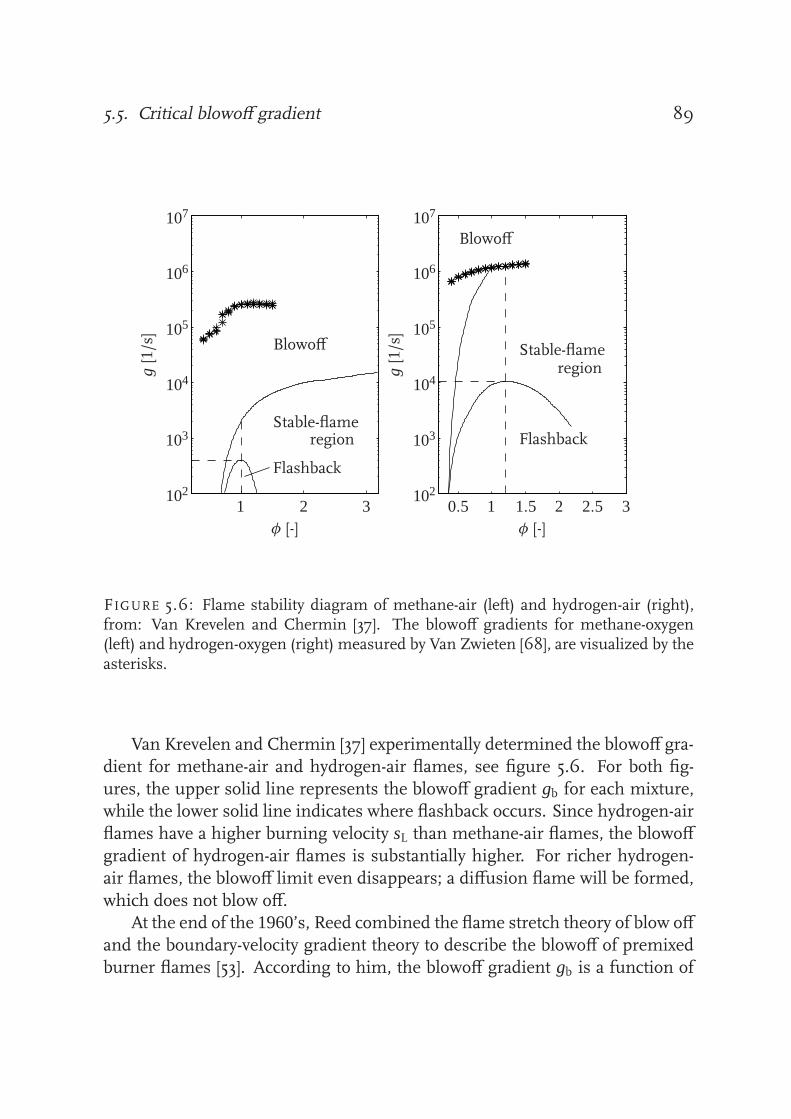
5.5. Critical blowoff gradient 89
g[1/s]
g[1/s]
φ [-]φ [-]
Blowoff
Blowoff Stable-flame
Stable-flame
region
region Flashback
Flashback
102102
103103
104104
105105
106106
107107
0.5 11 1.5 22 2.5 33
FIGURE 5.6: Flame stability diagram of methane-air (left) and hydrogen-air (right),from: Van Krevelen and Chermin [37]. The blowoff gradients for methane-oxygen(left) and hydrogen-oxygen (right) measured by Van Zwieten [68], are visualized by theasterisks.
Van Krevelen and Chermin [37] experimentally determined the blowoff gra-
dient for methane-air and hydrogen-air flames, see figure 5.6. For both fig-
ures, the upper solid line represents the blowoff gradient gb for each mixture,while the lower solid line indicates where flashback occurs. Since hydrogen-air
flames have a higher burning velocity sL than methane-air flames, the blowoff
gradient of hydrogen-air flames is substantially higher. For richer hydrogen-
air flames, the blowoff limit even disappears; a diffusion flame will be formed,
which does not blow off.At the end of the 1960’s, Reed combined the flame stretch theory of blow off
and the boundary-velocity gradient theory to describe the blowoff of premixed
burner flames [53]. According to him, the blowoff gradient gb is a function of

90 Chapter 5. Practical applications
Flame front Fouling
a b c
FIGURE 5.7: Schematic overview of a glass product heated by an impinging flame jet;a: without fouling, b and c: with fouling.
the burning velocity sL as follows:
gb = 0.23ρcps2L
λ. (5.17)
Recently some experiments have been carried out to determine the blowoff
gradient gb of methane-oxygen and hydrogen-oxygen flames [23, 68]. In figure
5.6, the results are visualized with the asterisks. Methane-oxygen flames, hav-
ing a burning velocity sL which is 10 times higher than the burning velocity ofmethane-air flames, have a blowoff gradient gb which is 100 times higher than
the blowoff gradient of methane-air flames, as equation (5.17) indicates as well.
For hydrogen-oxygen flames, however, the flame thickness is not negligible as
for the methane-oxygen flames, and therefore the theory, assuming an infinite
small flame thickness, does not hold. As figure 5.6 shows, the blowoff gradientfor hydrogen-oxygen flames is higher than for methane-oxygen flames. Con-
sequently, with hydrogen-oxygen flames higher gas velocities can be achieved
than in the case of methane-oxygen flames and therefore more heat can be
transported to the product.
5.6 Burner fouling
Burner fouling is an important issue in glass heating processes. In practice,
burner fouling occurs as quartz vapor from the heated quartz product settles
on the burner, see figure 5.7. As a result, the heat flux from the impinging

5.6. Burner fouling 91
q
H
Rj
ab
c
FIGURE 5.8: Heat flux q as a function of flame tip-to-target distance H for differentvalues of the burnt gas jet radius Rj for a burner fed with an oxy-fuel mixture (solidlines). The direction of the arrow indicates an increasing value of Rj. The dashed linesrepresent the heat flux for the case that the burnt gas velocity is increased, the letters’a’, ’b’ and ’c’ refer to the situation visualized in figure 5.7.
flame jet to the target can be altered significantly, as will the pressure drop
over the burner. In this section it will be shown how fouling can alter the heattransfer qualitatively as an effect of change in configuration, while the effect of
pressure drop on the heat transfer will be neglected.
Figure 5.8 schematically shows the heat flux q as a function of the flame tip-
to-plate distance H for different values of the burnt gas jet radius Rj. The letters’a’, ’b’ and ’c’ correspond to the situation visualized in figure 5.7. Situation ’a’
depicts the situation where there is no fouling. In situation ’b’, quartz vapor
has settled on top of the burner. Consequently, the flame stabilizes on top of
the quartz dust resulting in a smaller flame tip-to-plate distance. Dependent
on how much the flame has moved up, the heat flux can be increased for thissituation, see figure 5.8.
Situation ’c’ represents the case that the quartz vapor has settled inside the
burner nozzle. Since the exit radius of the burner is reduced in this case, the

92 Chapter 5. Practical applications
burnt gas jet radius Rj decreases as well. Furthermore, since the outflowing
unburnt gas volume remains the same, the unburnt gas velocity and thereforethe burnt gas velocity increases. As figure 5.8 shows, both these effects result
in an increase of heat flux.
Chapter
6Summarizing conclusions
In this thesis the heat transfer of impinging oxy-fuel flame jets to glass productshas been studied. Prior to the investigation, two main research questions have
been posed, namely: How are the velocity and the jet width of the burnt gases after
expansion over the flame front related to the unburnt gas velocity and burner radius?
and Can existing relations for the heat transfer of impinging flame jets, which are
applicable to situations where the target is placed relatively far from the flame, beextended or reformulated so that they are applicable for small distances between the
flame and target as well?.
A relation has been derived between the burner radius and the unburnt gas
velocity on one hand and the burnt gas jet width and burnt gas velocity on the
other. Since these burnt gas properties serve as input parameters for heat-fluxcalculations, it is important to know the burnt gas properties when the heat
flux from impinging flame jets to glass products is being considered. An ide-
alized representation of the flame and flow characteristics has been utilized to
derive the relation between the unburnt and burnt gas parameters, where thevelocity profile exiting the burner nozzle is taken to be flat and where curvature
effects of the flame are assumed to be negligible. Furthermore, only the global
conservation equations of mass, momentum and energy have been taken into
account. Particle Image Velocimetry measurements have been applied to vali-
date the derived relation and shows good agreement with the model, especiallyfor the oxy-fuel flames under consideration.
An analytical relation for the convective heat flux from an impinging flame
jet to the hot spot of a glass product has been derived as well. The relation is
obtained by dividing the domain in two regions. In the region far away fromthe plate, viscosity is negligible and the flow is treated as a potential flow. In the
93
94 Chapter 6. Summarizing conclusions
region close to the plate, viscosity becomes a leading term. At the edge of the
viscous boundary layer, the solutions of both regions are coupled together. Thissolution shows a good agreement with existing semi-analytical relations which
are only applicable for relatively large distances between the flame tip and the
target. On top of that, the convective heat transfer for closer flame tip-to-plate
distances can be calculated as well. Subsequently, an extension of the analyticalconvective heat flux has been presented. Using this extension, the heat flux to
the target for larger radial distances from the hot spot can be determined. In
agreement with the analytical solution for the convective heat flux, experimen-
tal validation using thermometry techniques clearly shows that the heat flux is
independent of distance for larger flame tip-to-plate distances, while for closerspacings the heat flux increases significantly. The point of transition between
these two regions shows good agreement between the calculated value and the
experimentally determined value.
With the acquired knowledge about the heat transfer of an impinging flame
jet to a product, the understanding of the process has been enhanced. Fromthe presented heat-flux relations, it is clearly shown that regarding the distance
between the flame tip and the target, two regions can be distinguished: a region
where shifts in distance have no influence on the heat transfer and a region
where shifts in distance cause a large alteration in the heat flux. To obtain astable process where the reproducibility of glass products is high, it is advised
to place the target at such a distance from the flame tip, that shifts in distance
have little influence on the heat transfer. The difference between heating with
a hydrogen-oxygen flame and a methane-oxygen flame has been mentioned
briefly. Also the effect of fouling, being a problem in the heating process, canbe understood more qualitatively using the acquired knowledge.
One of the most important parameters in the heating process of glass prod-
ucts is the distance between the flame tip and the target, and therefore the
flame height. Using a simplified reproduction of the flame front, a relationfor the flame height has been presented. The effect of flame curvature, how-
ever, which is not taken into account in the derivation, causes a deviation from
this solution. An improvement of this solution, taking flame curvature into
consideration, is therefore recommended.
It has been shown that the unburnt gases of oxy-fuel flames mainly di-verge sideways after expansion over the flame front, causing a burnt gas veloc-
ity which is approximately the same as the unburnt gas velocity. It is advisable
to look into the possibility of enclosing the flame in the heating process, since

95
expansion sideways will be suppressed this way. Consequently, higher burnt
gas velocities can be obtained resulting in higher heat fluxes.

96 Chapter 6. Summarizing conclusions

Nomenclature
Roman symbols
a applied strain rate 1/scp specific heat at constant pressure J/(kg·K)Dh hydraulic diameter m
D species diffusivity coefficient m2/s
d diameter m
f friction factor -
gb critical boundary-velocity gradient at blowoff 1/sg gravitational acceleration m/(s2)
Hflame flame height m
Htot burner nozzle-to-plate distance m
H flame tip-to-plate distance m
H∗ critical distance m
h heat transfer coefficient W/(m2·K)hC chemical enthalpy J/kg
hS sensible enthalpy J/kg
hT total enthalpy J/kg
K loss factor due to outflow -
K strain rate of the burnt gases 1/sLe Lewis number -
L plate thickness m
l characteristic length scale m
97

98 Nomenclature
m mass flux kg/(m2·s)m mass kg
Nu Nusselt number -
n unity vector -
Pe Peclet number -
Pr Prandtl number -
P pressure tensor N/m2
p pressure N/m2
q heat flux W/m2
Re Reynolds number -
Ri Richardson number -
R radius m
R universal gas constant J/(mol·K)sL laminar burning velocity m/s
TCHR TCHR factor -
T temperature K
t time s
U uniform flow velocity m/s
u, v velocity components m/s
u velocity field m/s
v velocity field m/s
V velocity of the unburnt gases in the burner m/s
xδ viscous boundary layer thickness m
x, r cylindrical coordinates m
x, y Cartesian coordinates m
Greek symbols
α thermal diffusivity m2/s
α thermal expansion coefficient 1/Kβ velocity gradient 1/sγ turbulence-enhancement factor -
1 difference
λ thermal conductivity W/(m·K)

Nomenclature 99
µ dynamic viscosity kg/(m·s)ν kinematic viscosity m2/s
ρ density kg/m3
τ expansion coefficient -
τ stress tensor kg/(m·s2)
φ equivalence ratio -
Subscripts
0 referring to the hot side of the plate
b referring to burnt conditions
b referring to the burner
d referring to the diameter
eq referring to equilibrium conditions
flame referring to flame conditions
g referring to the gas
∞ referring to the free stream
j referring to the jet
q referring to the quartz
u referring to unburnt conditions
w referring to the stagnation point
Abbrevations
CFD Computational Fluid Dynamics
ICCD Intensified Charge-Coupled Device
MFC Mass Flow Controller
PIV Particle Image Velocimetry
PMT PhotoMultiplier Tube
TCHR Thermochemical Heat Release

100 Nomenclature

Appendix
ASolution of the convective heatflux for a two-dimensional case
In this appendix we present the derivation of the convective heat flux of an
impinging flame jet to a plate for a two-dimensinal case. The derivation will beconcise and analogous to the derivation of the convective heat flux for a two-
dimensional axisymmetric case, presented in chapter 3.
The situation is represented in figure A.1. We start from the conservation
equations of mass and momentum:
∂ρ
∂ t+ ∇ · (ρv) = 0, (A.1)
∂(ρv)
∂ t+ ∇ · (ρvv) = −∇ · P + ρg. (A.2)
The temperature T and density ρ are a function of the spatial coordinate xonly. Assuming an incompressible flow and using the ideal gas law, results in
the term ρT to be a constant. Using m = ρu and v = y · v(x), the continuity
equation now yields∂(ρu)
∂x= −ρK , (A.3)
where the strain rate K is a function of x only and equal to K = v = ∂v∂y .
Using p = p(x, y) and µ = µ(x), the following conservation equations x - andy-momentum now hold:
−mdu
dx+ d
dx
[
2
3µ
(
2du
dx− K
)]
+ µdK
dx= ∂p
∂x, (A.4)
mdK
dx+ ρK 2 − d
dx
(
µdK
dx
)
= −1
y
dp
dy. (A.5)
101
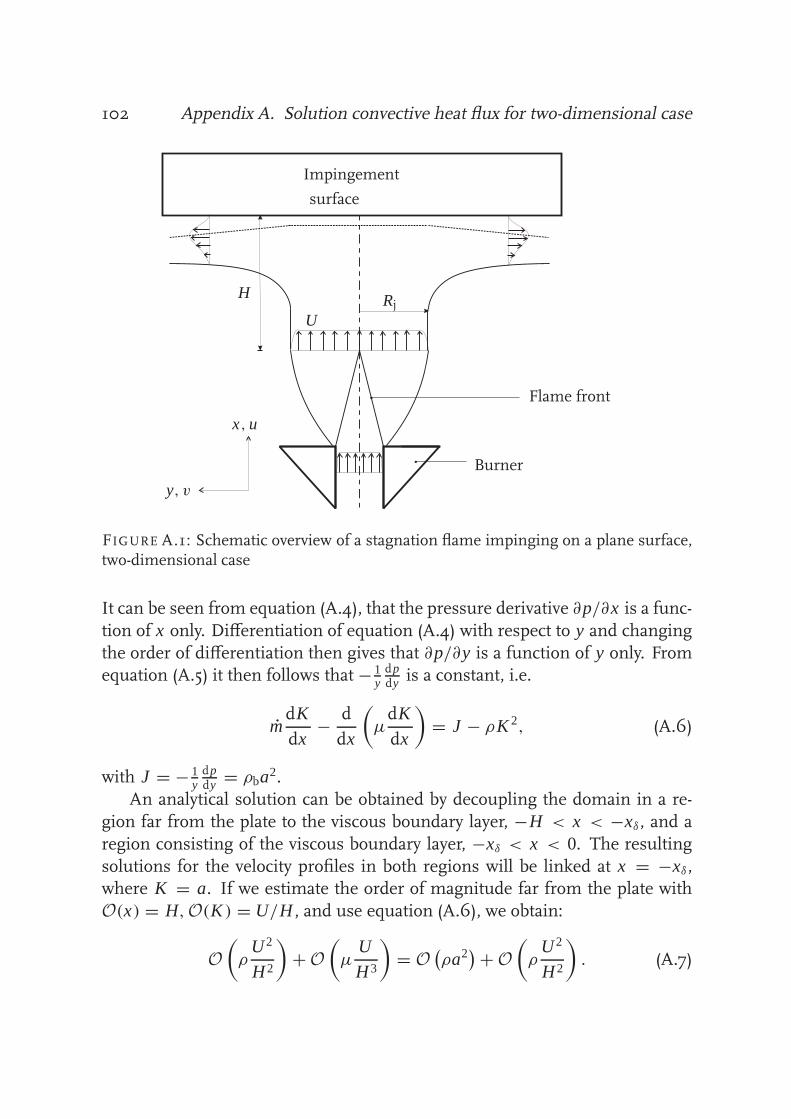
102 Appendix A. Solution convective heat flux for two-dimensional case
Flame front
Burner
Impingement
surface
H
URj
x, u
y, v
FIGURE A.1: Schematic overview of a stagnation flame impinging on a plane surface,two-dimensional case
It can be seen from equation (A.4), that the pressure derivative ∂p/∂x is a func-
tion of x only. Differentiation of equation (A.4) with respect to y and changing
the order of differentiation then gives that ∂p/∂y is a function of y only. Fromequation (A.5) it then follows that − 1
ydpdy is a constant, i.e.
mdK
dx− d
dx
(
µdK
dx
)
= J − ρK 2, (A.6)
with J = − 1ydpdy = ρba2.
An analytical solution can be obtained by decoupling the domain in a re-
gion far from the plate to the viscous boundary layer, −H < x < −xδ, and a
region consisting of the viscous boundary layer, −xδ < x < 0. The resulting
solutions for the velocity profiles in both regions will be linked at x = −xδ,where K = a. If we estimate the order of magnitude far from the plate with
O(x) = H,O(K ) = U/H , and use equation (A.6), we obtain:
O
(
ρU 2
H 2
)
+ O
(
µU
H 3
)
= O(
ρa2)
+ O
(
ρU 2
H 2
)
. (A.7)

103
Since O(a) = U/H , the viscous term is not relevant far from the plate if H ≫√ν/a. Far from the plate the density is constant. Using the continuity equation
(A.3), the relation between the strain rate K and the velocity u becomes:
K = −du
dx. (A.8)
Using equation (A.8), equation (A.6) is now reduced to:
−uu′′ = a2 − u′2. (A.9)
The solution for this equation can be obtained analytically. The boundary con-
ditions at x = −H are u = U and K = −du/dx = 0. Using these boundary
conditions, the following solutions for the velocity profile and strain profile canbe found:
u(x) = U sin
(−ax + xrefU
)
, (A.10)
K (x) = a cos
(−ax + xrefU
)
, (A.11)
where a = πU/(2H) and the value of xref is determined by the boundary layer
thickness xδ. Equations (A.10) and (A.11) are valid for −H < x < −xδ, but alsofor the whole domain if the flow is non-viscous (xref = 0).
Close to the plate m and K become zero and equation (A.6) is reduced for
−xδ < x < 0 to
− d
dx
(
µdK
dx
)
= ρba2. (A.12)
At x = −xδ the strain rate K is maximum and equal to a ≃ πU2H . Using this
boundary condition and K (0) = 0, the strain rate K in the viscous boundary
layer can be calculated. Close to the plate, the density and velocity of the burnt
gas flow can be approximated by
ρ ∼ ρ0 + ρ ′x, u ∼ bx2,
with ρ0 the density of the burnt gas flow at the flame side of the plate and b aconstant. Since
ρdu
dx∼ 2bρ0x, u
dρ
dx∼ bρ ′x2,

104 Appendix A. Solution convective heat flux for two-dimensional case
and therefore ρdu/dx ≫ udρ/dx , the strain rate can be approximated by
K (x) = − ∂u∂x . The velocity solution in the boundary layer equals:
u(x) = axδ
(
x3
3x3δ
+ x2
x2δ
)
, (A.13)
with xδ =√
2µ/(ρa) =√
2ν/a. The relations for the velocity, equations (A.10)and (A.13) are linked by the condition that the strain rate at x = −xδ must equal
K = a = πU2H . Now xref can be calculated and equation (A.10) becomes:
u(x) = U sin
(−a(x + xδ/3)
U
)
. (A.14)
The convective heat flux can be calculated via a balance of conduction andconvection. The conservation equation is given by
ρucp∂T
∂x= ∂
∂x
(
λ∂T
∂x
)
. (A.15)
Substituting the equations for the velocity u (A.10) and (A.13) results in rela-tions for the heat transfer from the burnt gas flow to the glass product. First
we determine the heat transfer for a non-viscous gas flow (xδ = 0). We assume
both λ and the thermal diffusivity α = λ/(ρcp) to be constant. After substitut-
ing q = λdT/dx , the conservation equation of energy (A.15) changes to:
0∫
s
dq
q= 1
α
0∫
s
udx, (A.16)
which after integration results in the following equation for q:
q(s) = q0 exp
− 1
α
0∫
s
udx
. (A.17)
Equation (A.17) can be made dimensionless using x ′ = x/H . After integration
over the whole domain −H < x < 0 and substituting equation (A.10) for the
velocity profile u, the solution for the non-viscous heat transfer from the burnt

105
gases to the plate q0 is given by
q0 = λdT
dx
∣
∣
∣
0= λ(T0 − Tflame)
0∫
−Hexp
[
− 1α
0∫
sudx
]
ds
(A.18)
= λ(T0 − Tflame)
H0∫
−1exp
[
2π
Pe(
cos(
−π2 x ′)
− 1)]
ds ′. (A.19)
For this case, the integral in the denominator of equation (A.19) can be simpli-
fied using a Taylor expansion for the cosine. The heat transfer can be expressed
as follows:
q = λ∂T
∂x
∣
∣
∣
0= λ(T0 − Tflame)
1
H
√Pe. (A.20)
If we take viscosity into account to calculate the heat flux q0, we have to
make the distinction between the burnt gas flow region and the viscous bound-
ary layer again to calculate the denominator of equation (A.18). The denomina-
tor of equation (A.18) now becomes equal to
0∫
−H
exp
− 1
α
0∫
s
udx
ds =0∫
−xδ
exp
− 1
α
0∫
s
u2dx
ds+
−xδ∫
−H
exp
− 1
α
−xδ∫
s
u1dx +0∫
−xδ
u2dx
ds, (A.21)
where the velocity profile in the burnt gas flow region u1 is given by equation(A.10) and the velocity profile in the viscous boundary layer u2 by equation
(A.13). Implementing these velocity profiles in equation (A.21) and making
this equation dimensionless, results in the following denominator for equation

106 Appendix A. Solution convective heat flux for two-dimensional case
q(P
r)/q n
onvisc[-]
Pr [-]
0.7
0.75
0.8
0.85
0.9
0.95
1
1.05
0 0.2 0.4 0.6 0.8 1
FIGURE A.2: The ratio of the viscous heat flux and non-viscous heat flux as a functionof the Prandtl number. The dots represent the analytical results, the asterisks thenumerical results, the solid line the fit function y = exp
[
−0.28Pr0.40]
; H = 2 mm,R = 20 mm (two-dimensional case).
(3.19) for the viscous situation:
0∫
−H
exp
− 1
α
0∫
s
udx
ds =H
0∫
−xδ/H
exp
π2
96
Pe2
Prx ′4 + 1
12
√
Pe3π3
Prx ′3
ds ′+
H
−xδ/H∫
−1
exp
[
−1
2Pr − 2
πPe
(
cos
(
2
3
√
πPr
Pe
)
−
cos
(
−1
3
√
πPr
Pe− πx ′
2
))]
ds ′.
(A.22)
The ratio of the analytically calculated heat flux and the non-viscous heat
flux as a function of Pr is depicted using dots in figure A.2. The asterisks

107
2aH
/(π
U)[-]
H/Rj [-]
00
5
5
10
10
15
15 20 25 30
FIGUREA.3: Relation between 2aH/(πU) and H/Rj; the dots represent the numericalcalculations, the solid lines the functions 2aH/(πU) = 1 and 2aH/(πU) = H/(2Rj).
represent the ratio of the numerically calculated heat flux and the non-viscous
heat flux as a function of Pr. Therefore a distance to the plate of H = 2 mmand a plug width of R = 20 mm are chosen. The figure shows that the results
of the analytical and numerical calculations show good agreements. By fitting
a line through the analytical results, the heat transfer can be expressed as the
non-viscous heat transfer multiplied by a function of Prandtl:
q = qnon-viscous · f (Pr). (A.23)
The fit function of Prandtl is given by exp[
−0.28Pr0.40]
. Combining this with
equation (A.20), the heat transfer for the two-dimensional case can be expressed
as:
q = λ∂T
∂x
∣
∣
∣
0= λ(T0 − Tflame)
1
H
√Pe · exp
[
−0.28Pr0.40]
. (A.24)
Figure A.3 shows the numerical effect of the H/Rj ratio on the effective
strain rate of the burnt gases a. The factor 2aH/(πU) is set out as function
of H/Rj. The figure shows that for small H/Rj values, 2aH/(πU) is equal to
108 Appendix A. Solution convective heat flux for two-dimensional case
one. Furthermore, for a H/Rj ratio of 4 and higher and a fixed width of the
flow Rj and velocity U , the distance to the glass product H has no influenceon the strain rate a. The strain rate a now is a constant, represented by the
straight line indicating that 2aH/(πU) ∼ H/Rj or a = πU/(4Rj) independent
of H . We can now adjust equation (A.22) to make it valid not only for H/Rj < 1but for the complete H/Rj range. The two straight lines in figure A.3 intersectat H/Rj = 2. Since the strain rate is independent of the distance H for a
ratio of H/Rj larger than 2, the strain rate for large H/Rj ratios can be defined
as a = πU/(4Rj) = πU/(2H∗). The critical distance H∗ is defined here as
H∗ = 2Rj. Equation (A.22) now can be written as:
0∫
−H∗
exp
− 1
α
0∫
s
udx
ds =H∗0∫
−xδ/H∗
exp
π2
96
Pe2
Prx ′4 + 1
12
√
Pe3π3
Prx ′3
ds ′+
H∗−xδ/H∗∫
−1
exp
[
−1
2Pr − 2
πPe
(
cos
(
2
3
√
πPr
Pe
)
−
cos
(
−1
3
√
πPr
Pe− πx ′
2
))]
ds ′,
(A.25)
with
H∗ ={
H for H < 2Rj
2Rj for H ≥ 2Rj(A.26)
and Pe = U H∗/α. In the same way, equation (A.24) can be written as:
q = λ∂T
∂x
∣
∣
∣
0= λ(T0 − Tflame)
1
H∗
√Pe · exp
[
−0.28Pr0.40]
. (A.27)

References
[1] S.W. Allison, G.T. Gillies, Remote Thermometry with ThermographicPhosphors: Instrumentation and Applications, Review of Scientific Instru-
ments 68:7, 1–36 (1997).
[2] S.W. Allison, D.L. Beshears, T. Bencie, W.A. Hollerman and P. Boudreaux,
Development of temperature sensitive paints for high temperature aeropropul-
sion applications, AIAA-2001-3528, 2001.
[3] C.E. Baukal, B. Gebhart, A Review of Flame Impingement Heat Transfer
Studies - Part 1: Experimental Conditions, Comb. Sci. Tech., 1995 Vol. 104,
339–357.
[4] C.E. Baukal, B. Gebhart, A Review of Flame Impingement Heat Transfer
Studies - Part 2: Measurements, Comb. Sci. Tech., 1995 Vol. 104, 359–385.
[5] C.E. Baukal Jr., B. Gebhart, A Review of Empirical Flame Impingement
Heat Transfer Correlations, Int J Heat Fluid Flow, 17: 386–396, 1996.
[6] C.E. Baukal, B. Gebhart, A Review of Semi-Analytical Solutions for Flame
Impingement Heat Transfer, Int. J. Heat Mass Transfer, 39 (14), 2989–3002, 1996.
[7] C.E. Baukal, B. Gebhart, Surface Condition Effects on Flame Impinge-
ment Heat Transfer, Therm. Fluid Sci., 15 (1997), 323–335.
[8] C.E. Baukal, B. Gebhart, Heat transfer from oxygen-enhanced/natural gas
flames impinging normal to a plane surface, Exp. Therm. Fluid Sci., 16
(1998) 247–259.
109
110 References
[9] C.E. Baukal, jr., Heat Transfer in Industrial Combustion, CRC Press LLC,
Boca Raton (2000).
[10] W.J. Beek, K.M.K. Muttzall, J.W. van Heuven, Transport Phenomena, John
Wiley & Sons, LTD, second edition (1999).
[11] J.M. Beér, N.A. Chigier, Impinging Jet Flames, Combust. Flame, 12, 575–
586, 1968.
[12] A. Bejan,Heat Transfer, JohnWiley & Sons, Inc., 1993, ISBN 0-471-50290-
1.
[13] M.A. Cappelli, P.H. Paul, An Investigation of Diamond Film Deposition
in a Premixed Oxyacetylene Flame, J. Appl. Phys., 67 (5), 2596–2602,1990.
[14] http://w3.wtb.tue.nl/nl/organisatie/combustion_technology/flamecodes/
chem1d/ (2006).
[15] R. Conolly, R.M. Davies, A Study of Convective Heat Transfer fromFlames, Int. J. Heat Mass Transfer, 15 (1972), 2155–2172.
[16] M.F.G. Cremers, M.J. Remie, K.R.A.M. Schreel, L.P.H. de Goey, Heat
Transfer Mechanisms of Laminar Hydrogen+Oxygen Flames, Combust.
Flame, 139 (2004), 39–51.
[17] M.F.G. Cremers, Heat Transfer of Oxy-Fuel Flames to Glass - The Role ofChemistry and Radiation, Ph.D. thesis, Eindhoven University of Technol-
ogy, 2006.
[18] M.F.G. Cremers, M.J. Remie, K.R.A.M. Schreel, L.P.H. de Goey, Thermo-
chemical Heat Release of Laminar Stagnation Flames of Fuel and Oxygen,in preparation (2007).
[19] L.L. Dong, C.W. Leung, C.S. Cheung, Heat transfer of a row of three bu-
tane/air flame jets impinging on a flat plate, International Journal of Heat
and Mass Transfer 46 (2003) 113–125.
[20] L.L. Dong, C.W. Leung, C.S. Cheung, Heat transfer and wall pressure
characteristics of a twin premixed butane/air flame jets, Int. J. Heat Mass
Transfer 47 (2004) 489–500.
References 111
[21] J.A. Fay, F.R. Riddel, Theory of Stagnation Point Heat Transfer in Dissoci-
ated Air, J. Aero. Sci, 25 (1958), 73–85.
[22] http://www.fluent.com (2006).
[23] M. Gerth, Flame stabilization for oxy-fuel flames, MSc. Thesis, Eindhoven
University of Technology, Rep. nr. WVT 2004.13 (2004).
[24] W.H. Giedt, L.L. Cobb, E.J. Russ, Effect of Hydrogen Recombinationon Turbulent Flow Heat Transfer, ASME Paper 60-WA-256, New York
(1960).
[25] G.K. Hargrave, M. Fairweather, J.K. Kilham, Force Convective Heat Trans-
fer from Premixed Flames - Part 2: Impingement Heat Transfer, HeatFluid Flow, 8 (2), 132–138, 1987
[26] M.E. Horsley, M.R.I. Purvis, A.S. Tariq, Convective Heat Transfer from
Laminar and Turbulent Premixed Flames, Heat Transfer, Vol. 3, Hemi-
sphere, Washington, DC, (1982), 409–415.
[27] A. Ivernel, P. Vernotte, Etude Expérimentale de l’Amélioration des Trans-
fert Convectis dans les Fours par Suroxygénation du Comburant, Rev. Gén.
Therm., Fr., 210–211 (1979) 375–391.
[28] E.G. Jackson, J.K. Kilham, Heat Transfer from Combustion Products by
Forced Convection, Ind. Engng. Chem., 48 (11), 2077–2079, 1956.
[29] W.S. Janna, Design of Fluid Thermal Systems, PWS Publishing Company,
1993, ISBN 0-534-93373-4.
[30] W.M. Kays, Convective heat and mass transfer, McGraw-Hill, New York
(1966).
[31] R.J. Kee, J.A. Miller, A structured approach to the computational modeling
of chemical kinetics and molecular transport in flowing systems, Springer
Series in Chemical Physics 47:196 (1986).
[32] R.J. Kee, J.A. Miller, G.H. Evans, G. Dixon-Lewis, A computationalmodel of the structure and extinction of strained opposed-flow premixed
methane-air flames, 22nd Symposium (International) on Combustion, The
Combustion Institute, 1989, 1479–1494.

112 References
[33] J.K. Kilham, P.G. Dunham, Energy Transfer from Carbon Monoxide
Flames, Proceedings of Eleventh International Symposium on Combustion,The Combust. Instit., Pittsburg, PA, (1967), 899–905.
[34] J.K. Kilham, M.R.I. Purvis, Heat Transfer From Normally Impinging
Flames, Combust. Sci. Technology, Vol. 18 (1978), 81–90.
[35] C.R. Kleijn, Heat Transfer from Laminar ImpingingMethane/Air Flames,
Computational Technologies for Fluid/Thermal/Structural/Chemical Systems
With Industrial Applications, Volume 1, 259–269, ASME 2001.
[36] V. Kottke, H. Blenke, K.G. Schmidt, Messung und Berechnung des or-tlichen und mittleren Stoffübergangs an stumpf angestromten Kreiss-
cheiben bei unterschiedlicher Turbulenz, Wärme und Stoffübertragung
(1977), 10, 89–105.
[37] D.W. van Krevelen, H.A.G. Chermin, Generalized flame stability diagram
for the prediction of interchangeability of gases, Seventh Symposium on
combustion, 358–368.
[38] L.C. Kwok, C.W. Leung, C.S. Cheung, Heat transfer characteristics of slotand round premixed impinging flame jets, Exp. Heat Transfer 16 (2003)
111–137.
[39] L.C. Kwok, C.W. Leung, C.S. Cheung, Heat transfer characteristics of an
array of impinging pre-mixed slot flame jets, Int. J. Heat Mass Transfer 48(2005) 1727–1738.
[40] Lewis, Von Elbe, Combustion, flames and explosions of gases. Academic
Press Inc., New York and London, second edition, 1961.
[41] H. Martin, Heat and Mass Transfer Between Impinging Gas Jets and Solid
Surfaces, Adv. Heat Transfer, 13 (1977), 1–60.
[42] http://www.mathworks.com/access/helpdesk/help/techdoc/ref/
pdepe.html (2005).
[43] T.H. van der Meer, Heat Transfer From Impinging Flame Jets, Ph.D. thesis,
Delft University of Technology, 1987.

References 113
[44] A. Milson, N.A. Chigier, Studies of Methane-Air Flames Impinging on a
Cold Plate, Combust. Flame, 21, 295–305, 1973.
[45] K. Mizuno, R. Mital, R. Viskanta, An Experimental Study of Premixed
Flame Impingement Heat Transfer, Proceedings of the ASME Heat Transfer
Division, Eds. D.W. Pepper et al., Vol. 4, HTD-Vol. 335, ASME, New-York,
245–252, 1996.
[46] S. Nawas, Heat Transfer from Oxygen Enriched Methane Flames, Ph.D. The-
sis, The University of Leeds, Leeds, United Kingdom (1973).
[47] A. Omrane, G. Juhlin, M. Aldén, G. Josefsson, J. Engtström, T. Benham,
Demonstration of two-dimensional temperature characterization of valvesand transparent piston in a GDI optical engine, SAE, 2004-01-0609.
[48] Alaa Omrane, Thermometry Using Laser-Induced Emission from Thermo-
graphic Phosphors: Development and Applications in Combustion, PhD-
thesis, Lund Institute of Technology (2005).
[49] N. Peters, Turbulent Combustion, Cambridge University Press, 2000,ISBN 0 521 66082 3.
[50] http://www.pivtec.com/
[51] S. Polat, B. Huang, A.S. Majumdar, W.J.M. Douglas, Numerical Flow and
Heat Transfer Under Impinging Jets: A Review, Ann. Rev. Num. FluidMech. Heat Transfer, 2, 157–197,1989.
[52] Cz. O. Popiel, Th. H. van der Meer, C.J. Hoogendoorn, Convective Heat
Transfer on a Plate in an Impinging Round Hot Gas Jet of Low Reynolds
Number, Int. J. Heat Mass Transfer, 23 (1980), 1055–1068.
[53] S.B. Reed, Flame stretch - a connecting principle for blowoff data, Com-
bust. Flame, 11-3 1967, 177–189.
[54] M.J. Remie, M.F.G. Cremers, K.R.A.M. Schreel, L.P.H. de Goey, Analysis
of the Heat Transfer of an Impinging Laminar Flame Jet, Int. J. Heat MassTransfer, accepted for publication.
[55] M.J. Remie, M.F.G. Cremers, K.R.A.M. Schreel, L.P.H. de Goey, Flame Jet
Properties of Bunsen-Type Flames, Combust. Flame, 147 (2006) 163–170.

114 References
[56] M.J. Remie, Heat Transfer from Flames to a Quartz Plate, MSc. Thesis,
Eindhoven University of Technology, Rep. nr. WVT 2002.01 (2002).
[57] J.R. Rigby, B.W. Webb, An Experimental Investigation of Diffusion Flame
Jet Impingement Heat Transfer, Proc. ASME/JSME Thermal Engineering
Joint Coference 1995, Eds. L.S. Fletcher and T. Aihara, Vol. 3, ASME, New
York, 117–126.
[58] D.E. Rosner, Convective Heat Transfer with Chemical Reaction, Aeron.
Res. Lab. Rept ARL 99, Part 1, AD269816 (1961).
[59] H. Seyfried, G. Särner, A. Omrane, M. Richter, H. Schmidt, M. Aldén, Op-
tical diagnostics for characterization of a full-size fighter-jet afterburner,Proceedings of ASME GT2005, GT2005-69058.
[60] P.S. Shadlesky, Stagnation point heat transfer for jet impingement to a
plane surface, AIAA Journal 21 (8) (1983) 1214-1215.
[61] M. Sibulkin, Heat transfer near the stagnation point of a body of revolu-
tion, J. Aeron. Sci., 19 (1952) 570–571.
[62] G. Stahl, J. Warnatz, Numerical Investigation of Strained Premixed CH4-
air Flames up to High Pressures, Combust. Flame, 85:285.
[63] W. Stutzenberger, Konvektiver Wärmeübergang von Brenngas-Sauerstoff-
Flammen an Gekühlte und Sich Erwärmende Metalloberflächen, Doktor-Ingenieur Dissertation, Ruhr-Universität Bochum, Bochum, Germany.
[64] R. Viskanta, Heat transfer to Impinging Isothermal Gas and Flame Jets,
Exper. Therm. Fluid Sci., 1993, 6:111–134.
[65] R. Viskanta, Overview of Flame Impingement Heat Transfer: Fundamen-tals and Applications, Adv. Heat Transfer Eng., Proc. of the Fourth Baltic
Heat Transfer Conference (2003), 143–158.
[66] R. Viskanta, Convective and Radiative Flame Jet ImpingementHeat Trans-
fer, I. J. Transport Phenomena, 1 (1998), 1–15.
[67] Z. Zhao, T.T. Wong, C.W. Leung, Impinging premixed butane/air circu-
lar laminar flame jet - influence of impingement plate on heat transfer
characteristics, Int. J. Heat Mass Transfer 47 (2004) 5021–5031.

References 115
[68] F. van Zwieten, Blow-off of oxy-fuel flames and air-fuel flames, Bachelor fi-
nal project, Eindhoven University of Technology, Rep. nr. WVT 2005.16(2005).

116 References

Abstract
Impinging flame jets are commonly used in glass heating processes for cutting,
melting and forming purposes. High local heat-transfer rates can be obtained
using these flame jets which is preferable, since the processing times of glass
products need to be short. To increase the heat-transfer rates, the burners areoften supplied with a pure fuel-oxygen mixture resulting in high flame temper-
atures and high gas velocities compared to a fuel-air mixture. However, flame
impingement is a very complex process where fluid dynamics, thermodynam-
ics and chemical kinetics all play an important role. These phenomena needdeeper understanding before the process can be analyzed, to avoid high ther-
mal stresses and overheating of the hot spots of the glass products.
Four regions can be distinguished in the flow structure of an impinging
flame jet: a flame jet region, a free jet region, a stagnation region and a wall
jet region. Since the typical time scales of the regions differ, each region canbe decoupled, treated separately and coupled again afterwards. Generally, the
impinging flame jet is placed close to the product resulting in a laminar burnt
gas flow. Since the shell thickness of the glass tubes is significantly smaller
than the radius of the tubes, the glass product can be approximated by a flat
plate.A relation has been derived which relates the burner radius and the un-
burnt gas velocity on the one hand to the burnt gas jet radius and the burnt
gas velocity on the other. By that, the relation couples the flame jet region to
the free jet region. An idealized reproduction of the flame front has been used,where the effect of flame curvature was neglected and where the velocity profile
at the exit of the burner nozzle was assumed to be flat. By solving the global
conservation equations of mass, momentum and energy, the relation between
the above mentioned parameters was derived. Experimental validation using
Particle Image Velocimetry showed good agreement, especially for the oxy-fuel
117

118 Abstract
flames under consideration.
An analytical relation for the convective heat flux from the burnt gases inthe free jet region and the stagnation region to the hot spot of the glass product
has been derived. In agreement with existing semi-analytical relations, this
new relation shows that for high flame tip-to-plate distances, the convective
heat flux is constant. The difference, however, is that with the new relation theheat flux for shorter distances can be determined as well. For these shorter
distances between the flame tip and the product, the heat flux is very sensitive
to small shifts in distance. Phosphor thermometry measurements confirm the
derived behavior.
The heat-flux relation has been extended to radial distances further awayfrom the hot spot based on numerical studies. Hence, this extension provides
the heat flux from the burnt gases in the wall jet region to the glass product.
Using this relation as a boundary condition offers the possibility to calculate
the temperature distribution inside the product, without solving the flow field
of the flame jet. Experimental validation with phosphor thermometry measure-ments show good agreement again.
With the acquired knowledge on flame-impingement heating, a better un-
derstanding of the process is gathered. Knowing the gas parameters and con-
figuration, the heat flux of an impinging jet can be determined. Furthermore,the effects of changes in geometry and/or fuel can be predicted and explained.
Taking the presented single-flame configuration as a starting point, extension
to more complex geometries looks promising.

Samenvatting
In de verschillende stadia van lampproductieprocessen worden branders toe-
gepast om glasproducten lokaal te kunnen bewerken. Hierdoor wordt de hoge
warmteoverdracht bereikt die nodig is om korte procestijden te kunnen garan-
deren. Om een nog hogere warmteoverdracht te bewerkstelligen, worden debranders vaak gevoed met een puur zuurstof-brandstofmengsel, wat resulteert
in hoge vlamtemperaturen en hoge gassnelheden ten opzichte van lucht-brand-
stofmengsels. Fenomenen als stromingsleer, thermodynamica en chemische
kinetiek spelen in dit warmteoverdrachtsproces alle een belangrijke rol en het
warmteoverdrachtsproces is daardoor zeer complex. Om het proces te kunnenanalyseren, moet het effect van elk van deze fenomenen onderzocht worden
zodat te hoge thermische spanningen in en het oververhitten van de glaspro-
ducten vermeden kunnen worden.
In het stromingsgebied van een vlam die een glasproduct verwarmt, kun-
nen vier domeinen onderscheiden worden: het domein waarin zich de vlambevindt, het domein waardoor de verbrande gassen stromen en waar het pro-
duct nog geen invloed heeft op deze stroming, het domein waarin de stro-
ming stagneert als gevolg van de aanwezigheid van het product en het domein
grenzend aan het product waardoor de verbrande gassen van het product afstromen. Aangezien de typische fysische tijdschaal in elk domein verschilt,
kunnen deze domeinen ontkoppelt, vervolgens apart behandeld en uiteindelijk
weer aan elkaar gekoppeld worden. In het algemeen worden de branders der-
mate dicht bij het product geplaatst, dat de stroming van de verbrande gassen
laminair is. Aangezien de wanddikte van de glasbuizen aanzienlijk kleiner isdan de straal van de buizen, kunnen de glasproducten door een vlakke plaat
benaderd worden.
Een relatie is afgeleid tussen de branderuitstroomradius en de onverbrande
gassnelheid enerzijds en de radius van de verbrande gasjet en de verbrande
119

120 Samenvatting
gassnelheid anderzijds. Met deze relatie worden oplossingen in het vlam-
domein en het domein waardoor de verbrande gassen stromen met elkaar ver-bonden. Om tot deze relatie te komen, is gebruik gemaakt van een geïdeali-
seerde weergave van het vlamfront, waarbij krommingseffecten geen rol spe-
len en waar het uitstroomprofiel van de onverbrande gassen bij de branderuit-
stroomopening vlak is. Verder zijn alleen de globale behoudsvergelijkingenvan massa, impuls en energie op het vlamdomein toegepast. Particle Im-
age Velocimetrymetingen zijn uitgevoerd om de verkregen relatie te valideren;
de resultaten vertonen, zeker voor de zuurstof-brandstofvlammen, een goede
overeenkomst.
Voor de warmteoverdracht van de verbrande gassen in de domeinen, waar-door de verbrande gassen stromen nog voor deze afbuigen als gevolg van de
aanwezigheid van het glasproduct, naar het gebied van impact van het glas-
product, is een analytische relatie afgeleid. Met deze relatie wordt aangetoond,
dat voor grotere afstanden tussen de vlamtip en het product, de warmteover-
dracht constant is; dit is in overeenstemming met bestaande semi-analytischerelaties. Het grote verschil is echter, dat met deze nieuwe relatie de warm-
teoverdracht ook berekend kan worden als het product dichter bij de vlamtip
geplaatst wordt. Voor deze situatie zal de warmteoverdracht sterk variëren als
het product ook maar een klein beetje richting de vlamtip of van de vlamtip afbewogen wordt. Phosphor thermometrymetingen bevestigen het gedrag resul-
terend uit de berekeningen.
Bovengenoemde relatie is zodanig uitgebreid, dat deze ook voorspelt wat
de warmteoverdracht is van de verbrande gassen die door het gebied gren-
zend aan en van het product af stromen. Door deze warmteoverdrachtsre-latie als een randvoorwaarde te gebruiken, kan de temperatuursverdeling in
een glasproduct berekend worden, zonder ook de stroming van de verbrande
gassen te moeten berekenen. Validatie middels phosphor thermometrymetin-
gen vertoont een goede overeenkomst.Met dit onderzoek zijn verbeterde inzichten verkregen in het warmteover-
drachtsproces van zuurstof-brandstofvlammen naar glasproducten. Als de gas-
parameters en de configuratie van het proces bekend zijn, kan de warmteover-
dracht van de vlammen berekend worden. Bovendien kunnen de effecten
van veranderingen in geometrie en/of brandstof voorspeld en verklaard wor-den. Tenslotte kan de gepresenteerde enkele brandergeometrie als beginpunt
genomen worden, om complexere geometrieën te bestuderen.

Curriculum Vitae
4 November 1976 Born in Breda.
Aug. 1989 - June 1995 Pre-university education (VWO),
Sint-Oelbertgymnasium, Oosterhout.
Sept. 1995 - June 1999 Mechanical Engineering,
Polytechnical Faculty West-Brabant,
Breda, B.Sc. degree.
Sept. 1999 - Aug. 2002 Mechanical Engineering,
Eindhoven University of Technology,
M.Sc. degree.
Aug. 2002 - Feb. 2007 Ph.D. student,
Eindhoven University of Technology,
Faculty of Mechanical Engineering,
Combustion Technology Group.
Journal publications following from this thesis
[1] M.J. Remie, M.F.G. Cremers, K.R.A.M. Schreel, L.P.H. de Goey, Flame Jet
Properties of Bunsen-Type Flames, Combust. Flame, 147:163–170 (2006).[2] M.J. Remie, M.F.G. Cremers, K.R.A.M. Schreel, L.P.H. de Goey, Analysis
of the Heat Transfer of an Impinging Laminar Flame Jet, Int. J. Heat Mass
Transfer, accepted for publication (2006).[3] M.J. Remie, G. Särner, M.F.G. Cremers, A. Omrane, K.R.A.M. Schreel,
L.E.M. Aldén, L.P.H. de Goey, Extended Heat Transfer Relation for an Im-
pinging Laminar Flame Jet to a Flat Plate, under review (2007).
121

122 Curriculum Vitae
[4] M.J. Remie, G. Särner, M.F.G. Cremers, A. Omrane, K.R.A.M. Schreel,
L.E.M. Aldén, L.P.H. de Goey, Heat Transfer Distribution for an ImpingingLaminar Flame Jet to a Flat Plate, in preparation (2007).

Dankwoord
Nu het einde in zicht is van dit promotieonderzoek, wil ik graag een aantal
mensen bedanken die hebben meegeholpen aan een goede afronding. Uiter-
aard geen kleine taak, aangezien ik me bewust ben van het feit dat dit het laat-
ste, maar in de praktijk vaak het eerst gelezen hoofdstuk is en ik niemand wilvergeten.
Allereerst wil ik mijn promotor Philip de Goey bedanken. Elke keer als ik
door de bomen het bos niet meer zag, wist hij ingewikkelde problemen weer tot
iets eenvoudigs te herleiden zodat ik weer vol goede moed kon werken naar deoplossingen. Ook met mijn co-promotor Koen Schreel heb ik bijzonder prettig
kunnen samenwerken; als ik ergens vastzat en dit soms in minder genuan-
ceerde bewoordingen duidelijk maakte, nam hij telkens de tijd om alles rustig
te analyseren, waarna we er altijd wel weer uitkwamen.
Gedurende het project heb ik nauw samengewerkt met Marcel Cremers.Naast de goede resultaten die we behaald hebben in dit project, was er ook
altijd tijd voor de nodige gein. Ook wil ik de overige projectleden van Philips
en in het bijzonder Richard Mikkers bedanken voor de vele zinvolle discussies,
de bezoeken aan de verschillende plants en de prettige samenwerking. Verder
heeft een aantal studenten mij in het kader van hun stage- of afstudeerprojectwerk uit handen genomen. Daarvoor wil ik Maarten, Joep, Lesley, Arno, Toon,
Francis, Ron en Sjoerd nogmaals bedanken. For the possibility to perform
some of the experiments described in this thesis, I would like to thank my
second ’promotor’ Marcus Aldén as well as Alaa Omrane and Gustaf Särnerfor their help during and after the measurements.
Uiteraard wil ik iedereen binnen de sectie Verbrandingstechnologie be-
danken die op de één of andere manier mee heeft geholpen om dit werk te
voltooien. In het bijzonder wil ikmijn kamergenotenMarcel, Edwin enMichael
bedanken voor de ontspannen sfeer en het feit dat op vrijdagmiddagen onze
123

124 Dankwoord
kamer toch wel met afstand de luidruchtigste was. Natuurlijk mag Marjan
niet ontbreken; bedankt voor de nodige theeleutsessies en uiteraard de relaxtemanier waarop we samen vele activiteiten binnen TFE hebben georganiseerd.
Tenslotte maar zeker niet op de laatste plaats wil ik mijn ouders bedanken
voor hun onvoorwaardelijke steun en het feit dat ze altijd voor me klaarstaan.
Iedereen bedankt voor een geweldige tijd!
Martin Remie, december 2006.