heat transfer simulation for thermal management of electronic...

Proceedings in Manufacturing Systems, Volume 11, Issue 1, 2016, 15‒26

ISSN 2067-9238

HEAT TRANSFER SIMULATION FOR THERMAL MANAGEMENT OF ELECTRONIC COMPONENTS

Tudor-George ALEXANDRU 1*, Theodor-Adrian MANTEA 2, Cristina PUPǍZǍ3, Ştefan VELICU 4

1) Eng., Machines and Manufacturing Systems Department, University "Politehnica" of Bucharest, Romania

2) PhD Student, Machines and Manufacturing Systems Department, University "Politehnica" of Bucharest, Romania 3, 4) Prof., PhD, Machines and Manufacturing Systems Department, University "Politehnica" of Bucharest, Romania

Abstract: The present research addresses electronics design issues with emphasis on the heat transfer simulations. The first part comprises a brief introduction to the electronics design workflow. The problem of the heat transfer is discussed at all engineering levels. Due to the complexity of this problem, multiphysics aspects remain in a close relationship with the thermal management systems. Such issues place the heat transfer simulation as a central design problem. Further decisions like economic, envi-ronmental, ergonomic or performance aspects remain sensitive to the solution of the heat transfer anal-yses. In the second part of the work, the heat transfer problem statement is described. Engineering knowledge achievements and their relationship with a PLM platform are schematically discussed. The most common heat transfer solvers are presented and the simulation peculiarities for the electronic com-ponents are emphasized. All this concepts are validated in the third part of the work, where two case studies are presented. First, an example of natural convection transfer for a heat sink was performed, in order to define theoretical aspects regarding the heat sink evaluation and to demonstrate how non-linear solvers based on the Finite Element Method can assess the transient temperature behavior. The second study was an experimental forced-convection steady-state cooling setup, simulated using Computational Fluid Dynamics. Numerical and experimental results for this simulation proved a good match. Conclud-ing remarks were highlighted at the end of the paper. Key words: electronics, design, cooling, heat transfer, knowledge, FEM, CFD.

1. INTRODUCTION 1

Heat transfer mechanism in electronics is a complex interdisciplinary subject that can be addressed at all de-sign stages in order to achieve the right decisions and the engineering knowledge for further development of the electronic products. The multiphysics aspect of the prob-lem can be divided in three main domains: the electric domain, the thermal domain and the fluid one [1]. Heat is generated in most electronics by active components due to the flow constraints applied to the electric current. Heat sinks, fans and blowers are used to take away the heat. Most electronics with moderate heat dissipation are fan cooled [2]. Apart from the passive aspect of the cool-ing, the active control aspect creates a balance between air or fluid flow in the fluid domain and the temperature of the components [3]. Optimal thermal management strategies lead to the avoidance of thermal cycling. In this way, lifetime expectancy and performance condi-tions of electronics are satisfied [4]. In the last decades power densities increased, while products became small-

* Corresponding author: 313 Splaiul Independentei Avenue, Bucha-rest 6, Romania Tel.: +40741041881; Fax: +40212691332; E-mail addresses: [email protected] (T.G. Alexandru), [email protected] (T.A. Mantea), [email protected] (C. Pupaza), [email protected] (S. Velicu)

er. The time between product acquisition and disposal has also decreased causing higher demands for electronic products. These aspects had an environmental side effect due to the waste stream produced every year [5]. Manu-facturing standards are continuously improving and manufacturers have to keep the pace [6]. Functional solutions are available to the electronics designs that are smaller and cooler. Heat sinks that combine heat pipes, micro channels with highly thermo conductive materials can replace conventional coolers [7]. Nanotechnology and the use of nano-silver in active components can de-crease temperatures and increase performances. Even though, the economical aspect can turn into a concern as the final products become expensive and their manufac-turers are no longer competitive [8]. Optimal electronics answer several multiphysics questions. The more engi-neering problems are solved, the better the product per-forms, becoming attractive to the market. The multiphysics aspect of the heat transfer makes the prob-lem sensitive to most design tasks. At circuit diagram level, the design is evaluated to determine a proper cool-ing solution. At assembly level, the components and the cooling are chosen according to the generated heat flow. At casing level, the agreed solution is fitted to accommo-date the air flow between the inlet and the outlet. At environmental level, both components and casing are required to satisfy standards. Any design decision is confirmed only after the heat transfer problem is solved for that scenario. The facts mentioned above, pointed out

16 T.G. Alexandru et al. / Proceedings in Manufacturing Systems, Vol. 11, Iss. 1, 2016 / 15−26

that heat transfer is a central design issue. The other design tasks revolve around this problem until thermal design specifications are complied.

Significant work was published in the field of heat transfer. The relationship between design tasks integrated in a collaborative platform for achieving design knowledge was described in [9]. Numerical 3D optimiza-tion of a heat sink base was performed in [10]. Computa-tional Fluid Dynamic (CFD) simulations were done to determine the thermal performances of nano-silver based components [11]. CFD studies were also presented for liquid-cooled heat sinks with microchannel flow field configurations to highlight thermal performances of different flow field configurations [12]. Combining nu-merical and analytical temperature approximation, a control algorithm was proposed in [13]. All these papers describe specific solutions for particular cases.

The present research comprises general guidelines and workflows that can be followed by design teams to achieve useful knowledge regarding the thermal man-agement of electronic components. Emphasizing the heat transfer issues, the first part of the work describes the design flows and suitable heat transfer solvers that can be used for different electronics designs. Important product information and the relationship with Product Life Cycle Management (PLM) solutions are also discussed. A comparison between two heat transfer numerical solu-tions is included in the second part of the paper. To prove the presented concepts, theoretical and experimental validated cooling problems are finally solved in the last part of the paper. These examples contain theoretical and experimental solutions that prove the accuracy of the presented concepts.

2. PROBLEM STATEMENT

In the field of electronics, competitiveness is a key factor to assure an optimal product price in respect to actual standards. Design engineers face multiple chal-lenges in order to take the right decisions. Optimal elec-tronics are designed with the least number of compo-nents, placed on an optimal Printed Circuit Board (PCB) layout and assembled in an ergonomic casing. The engi-neering knowledge is stored at PLM level and used fur-ther to automate simulation tasks, reuse models and share results. Due to the complexity of the electronics design, a wide range of software is used to capture multiphysics aspects of the product behavior. Circuit evaluation in electronics is used to study the constraints applied to the flow of the current within specific circuit elements. The conceptual design is tested using Electronic Design Automation software. The exterior and interior 3D as-sembly is completed by means of Computer Aided De-sign (CAD) software, with 3D files describing individual components and their geometrical constraints relative to each other. Engineers use numerical, analytical or com-bined heat transfer solutions to describe the thermal do-main. Optimal thermal assessments require a combina-tion of analytical solutions, empirical analysis and ther-mal modeling, using all available tools to support each other [14]. A wide range of heat transfer solvers are available. Analytical solvers require physical parameters of the derived equations. Thus, numerical solutions are

more common because complex parameters are not re-quired. Two types of commercial numerical heat transfer solvers are available: the Finite Element Method (FEM) and the CFD solver. Input data, boundary conditions, governing equations, convergence criteria and results are of different types for the two solvers. Therefore, a brief discussion is made further to highlight certain aspects: 2.1. FEM Solvers

Thermal analysis is used to determine the temperature distribution and the other heat transfer computations in a body: the quantity of heat exchanged, thermal gradient and heat flux [15]. As the structural response is influ-enced by the thermal field, coupled thermal-structural analysis are performed to describe the stress state due to thermal expansion or contraction.

In structural FEM based software, heat is transferred by conduction, convection (for 3D, 2D or axisymmetric structures that are in contact with a gas or fluid film) or through radiation [16].

Temperature distribution computation in electronics requires accurate material definition. It is also important that the solver has orthotropic material definition capabil-ities, due to the fact that a wide range of such materials are deployed in electronics (i.e. FR-4 epoxy composite used in PCBs). Results are particularly sensitive to the mesh. A coarser mesh can be applied outside the heat concentrators and an iterative local refinement can be accessed by means of adaptive meshing. This technique uses iterative 2D triangle or 3D tetrahedral mesh refine-ment. The resulting mesh might not have a good element quality, but the advantage is that the heat concentrators can be post-processed in depth.

The major disadvantage of the FEM thermal analysis is the size of the model and the computation time. While steady-state solutions can be achieved fast, transient solutions with applied adaptive mesh can take up to hours and the solution file can range from a few GB to hundreds of GBs, even for simple problems. 2.2. Computational Fluid Dynamics

CFD simulation tools combine cost-effective tools for simulating real flow by numerical solutions of the gov-erning equations. The resulting sets of equations are solved using computers by replacing partial differential equations with systems of algebraic equations [17]. The finite volume method used in CFD solvers computes the fluid flow and other related physical phenomena. Most processes of the forced convection cooling in electronics thermal management can be simulated using the CFD solvers. Instead of approximating convection film coeffi-cients as FEM software does, the CFD algorithm uses problem oriented solvers to determine the fluid flow between an inlet and an outlet. The major advantage on the FEM solution is the dedicated CFD pre and post-processors available for electronics. Simulation capabili-ties are expanded due to extended material libraries, components and Integrated Circuit (IC) package data-bases, multi-layer PCB configurators, thermal interface materials and others. Except heat dissipation, CFD solu-tions can post-process coolant velocity, pressure, effects of the flow rate or combined plane-cuts and volume-related results.

T.G. Alexandru et al. / Proceedings in Manufacturing Systems, Vol. 11, Iss.1, 2016 / 15−26 17

Fig. 1. PLM engineering knowledge in electronics. Nowadays, the mechanical engineers collaborate with

electronic engineers and with other research teams (i.e. environmental, quality assurance and others).

The general competence of the mechanical engineers in applications based on the heat transfer theory can simulate even the most peculiar cases, from the thermal management of simple micro-electronic circuits till the most complex control units deployed in the industry. Information from one application is transferred to anoth-er in one or two ways (Fig. 1). Each application auto-mates certain design tasks as described below: 2.3. Electronic Design Automation

At first, the circuit diagram of the assembly is created using Electronic Design Automation software for circuit evaluation and simulation purposes in the electrical do-main. The behavior of the current is captured and its transient flow can be described allowing all heat data to be estimated. Electronic Design Automation tools gener-ate the PCB product design and can also transfer neutral 3D CAD files independent or with the use of third-party tools, such as macros and add-ons. 2.4. Heat Transfer Calculator

The behavior of the electronic components can be used to compute 2D surface heat flow on 3D internal heat generation for components and printed circuits. Due to the complexity of the heat flow mechanism in elec-tronics (i.e. switching circuits, power losses, thermal characteristics, junction temperature, joule heating) a complete multiphysics description is still not available. Therefore, methods of computing thermal characteriza-tion parameters are based on simplified assumptions and

are offered as manufacturer guidelines [18]. Generally, these guidelines are for electronic components made by silicon chips and organic substrate, which generate heat. Recent designs presume smaller footprints and increased power densities. Technologies like nano-silver based circuits cannot be evaluated by conventional methods, because such components exhibit lower temperatures and higher performances. The study of these values can only be used to choose a preliminary cooling design. Engi-neers can also decide if the assembly requires passive (natural convection) or active (forced convection) cool-ing. The majority of electronics with moderate heat dis-sipation are fan cooled.

2.5. Computer Aided Design

Not all Electronic Design Automation applications have CAD generation features or extended component libraries (i.e. complex heat sinks, heat pipes, blowers, fans, specific connectors). Therefore, in order to com-plete the product assembly, a CAD system is required. Extensive interdisciplinary collaboration takes place at this stage. Design engineers decide on the casing, ergo-nomic studies are performed and reports are generated. Discussions take place between teams of design engi-neers and analysts. A final layout is proposed, than minor design changes are considered. For example, passive components can be placed in the vicinity of active com-ponents to act as heat exchangers. Also, small heat sinks can be positioned on the PCB under the active compo-nents, to enhance the thermal behavior around hot spots. This is only a preliminary design scenario where the 3D assembly is parameterized.

18 T.G. Alexandru et al.

Fig. 2. The central

The final decision will be taken after successive multiphysics analysis were both CAD and simulation parameters are improved. 2.6. Heat Transfer Solvers

Heat transfer solvers are used to predict the temperture of the components and parts within an assembly. The central role of the heat transfer codecapability of such software to identify any tpliance issues. Both hot spots within the PCB temperature distributions that exceed operational limits can be visualized. The choice of the heat ware ranges from simple analytical codenumerical solvers. Results from the heat transferto decide if the design is optimal or an optimization scnario has to be considered.

The concern of electronics heat transfer compuis that of the active components and their coolingcomponents (resistors, transistors, integrated circuitstransformers) are main heat sources. Heatthe highest possible heat flux, while the ture of the heatsink remains at low temperature. An otimal heatsink produces a uniform surface temperature with the least number of hot spots.

Based on the preliminary choice of ferent film coefficients are required to be computed. Predefined convection curves or approximation models can be used with an acceptable margin of error [Steps for computing film coefficients can be avoided when a CFD solver is used.

Numerical simulations analyze the temperature unformity, low average temperature of the heated supumping power assumptions, the effects of loss and other thermo-mechanical related phenomena. Both CFD and FEM are simulation tools that can be used to assess the thermal compliance of the electronic coponents. The necessary input data is the complete 3D model that is subjected to geometry simplifications. In the case of FEM, small holes, chamfers and other able features are removed. Complex packages are replaced with primitives (i.e. a cylinder can

Alexandru et al. / Proceedings in Manufacturing Systems, Vol. 11, Iss. 1, 2016 / 15

The central design problem of Heat transfer simulations.

n will be taken after successive

multiphysics analysis were both CAD and simulation

Heat transfer solvers are used to predict the tempera-components and parts within an assembly.

the heat transfer code (Fig. 2) is the capability of such software to identify any thermal com-

within the PCB layout or temperature distributions that exceed operational limits

heat transfer soft-ware ranges from simple analytical codes to complex

heat transfer are used an optimization sce-

heat transfer computation the active components and their cooling. Active

integrated circuits, rs) are main heat sources. Heatsinks remove

while the surface tempera-emains at low temperature. An op-

a uniform surface temperature

Based on the preliminary choice of the cooling, dif-ferent film coefficients are required to be computed.

or approximation models can be used with an acceptable margin of error [19]. Steps for computing film coefficients can be avoided

Numerical simulations analyze the temperature uni-formity, low average temperature of the heated surfaces, pumping power assumptions, the effects of the pressure

mechanical related phenomena. Both CFD and FEM are simulation tools that can be used to assess the thermal compliance of the electronic com-

a is the complete 3D subjected to geometry simplifications. In

the case of FEM, small holes, chamfers and other avoid-features are removed. Complex integrated circuit

with primitives (i.e. a cylinder can

replace a capacitor; a box can replace a chip). Where possible, combined surface and solid geometries are used and specific projections and cuts are generated to allow the solver to locally refine the mesh around the heat sources.

The CFD approach is similar to the FEM approach concerning the geometry. Primitives are alsreplace components. Both FEM and CFD programs use pre and post processing tools FEM programs are more general Representation procedures are available for multi-layer printed circuit boardelectronics pre and post processor for that can be intgrated with a FEM solver is Sherlock Automated Design Analysis™ software, from DfR hand, CFD solvers take advantage of aof electronics dedicated pre and post processors that simplify the components with automated replacement tasks. For example, fans are replaced wimesh.

In both FEM and CFD cases, are defined as lays of materialorientations. Compared to FEM, tact between two bodies requires conductance, CFD pre-processors include a dedicated Thermal Interface Material library that has all the themal conductivity characteristics pre

Both solvers can perform steady state or transient computations. The major difference between the two stands in the set of governing equations, the results thatcan be post-processed and thWhile the FEM method solves the basic equations ofheat transfer, CFD solvers for electronics solely on the cooling. Such programs can solve various fluid heat transfer linked problems by handling features and parts at angles and more complex shapes [complexity of the geometries used in electronics requiresdifferent turbulence models. For example, ANSYS ICEPAK can use one of eight turbulence availableels [22]: the zero-equation, the twok-ε) model, the Re-Normalisation Group

15−26

a box can replace a chip). Where possible, combined surface and solid geometries are used and specific projections and cuts are generated to allow the solver to locally refine the mesh around the heat

The CFD approach is similar to the FEM approach geometry. Primitives are also used to

Both FEM and CFD programs use pre and post processing tools devoted to electronics. FEM programs are more general heat transfer solvers. Representation procedures are available for modeling the

printed circuit board [20]. The only available electronics pre and post processor for that can be inte-grated with a FEM solver is Sherlock Automated Design Analysis™ software, from DfR Solutions. On the other

CFD solvers take advantage of an extended range of electronics dedicated pre and post processors that simplify the components with automated replacement tasks. For example, fans are replaced with 2D or 3D

d CFD cases, printed circuit boards of materials with different lay-up

Compared to FEM, where the thermal con-tact between two bodies requires the definition of the

processors include a dedicated library that has all the ther-

ty characteristics pre-defined. Both solvers can perform steady state or transient

computations. The major difference between the two stands in the set of governing equations, the results that

processed and the convergence criteria. While the FEM method solves the basic equations of the

for electronics are focused cooling. Such programs can solve various

problems by handling features and parts at angles and more complex shapes [21]. The

used in electronics requires different turbulence models. For example, ANSYS ICEPAK can use one of eight turbulence available mod-

equation, the two-equation (standard Normalisation Group k-ε model, the


realizable k-ε model, the enhanced two-equation (stand-ard k-ε with enhanced wall treatment) model, the en-hanced Re-Normalisation Group k-ε model, the enhanced realizable k-ε model, the Spalart-Allmaras model and the SST k-ω model, that is a two-equation eddy-viscosity model. Each type of turbulence model is used for solving different boundary condition problems. For example, the zero equations is appropriate for flows that are not dominated by recirculation regions, two-equation k-epsilon models are suitable for most forced convection problems and enhanced two equation solvers are recom-mended for near-wall complex phenomena.

In FEM problems, the convergence criteria are the heat and the temperature, while in CFD, the residuals are one of the most fundamental measures of an iterative solution convergence and it is used to quantify the error. The residual measures the local imbalance of a conserved variable. The numbers of iterations required for a good residual convergence depend on the type of the problem. Different turbulence solvers also use different residuals and convergence criteria. 3. THEORETICAL APPROACH

The equations for conductive heat transfer are de-scribed by [15]:

[ ] ][ QTKTC =⋅+⋅•

, (1)

where [ ]C represents the specific heat matrix, •

T ‒ time

derivative of the nodal temperatures, ][K ‒ thermal con-ductivity matrix, and Q ‒ the effective nodal heat flow

vector. The primary unknown values are the nodal tem-peratures. Other thermal parameters can be computed based on the nodal temperatures. There are two types of FEM thermal analysis: steady-state and transient thermal analysis.

3.1. Steady-state thermal analysis

Steady-state thermal analysis is used to determine the temperature distribution in a structure at thermal equilib-rium. Steady-state solvers assume that the loaded body instantaneously develops an internal field variable distri-bution to equilibrate the applied loads. The analysis is generally non-linear because the material properties are temperature dependent. The governing equations for a non-linear regime are:

iii QTK =+1][ , (2)

where i represents the iteration step number. The first iteration is used to solve the initial temperature condi-tions and the solution proceeds to the next iteration until the result convergence is achieved. The necessary num-ber of iterations for a precise solution depends on the non-linearity of the problem. For solving the non-linear problem Newton-Raphson algorithm is used. 3.2. Transient thermal analysis

This type of analysis is used to determine the temper-ature distribution within a structure as a function of time, to distribution within a structure as a function of time, to

predict the rates of the heat transfer, or the heat stored in the system [23]. The transient thermal analysis assumes the evolution of a new field variable distribution from a set of initial conditions via a set of transition states, evolving through time. Because most of the thermal phenomena have a transient evolution, this is the most common type of thermal simulation. Material properties for a transient thermal analysis are: the density, the ther-mal conductivity and the specific heat. The last charac-teristic is used to consider the effect of the stored heat:

[ ] iiiii QTKTC 11 =+ ++

•

, (3) where: [C] is the specific heat matrix and K ‒ matrix of the thermal conductivity.

Loads are functions of time. The effects of numerical integration are activated using the Crank-Nicholson, Euler and Galerkin or Backward stiffness methods. When the solution is done, post-processing of the tem-perature evolution in time can be presented as tables, graphs or contour plots.

3.3. CFD thermal analysis

The CFD simulation solves the conservation equa-tions for mass and momentum. For flows involving heat transfer, an additional equation for energy conservation is required [23].

The equation for mass conservation, or the continuity equation, can be written in a general form as follows [24]:

mSvt

=⋅∇+∂∂

)(ρρ

, (4)

where ρ is the fluid density, v

‒ speed vector, and Sm ‒ source mass.

The conservation of momentum in an inertial refer-ence frame is described by [25]

( ) Fgpvvvt

++⋅∇+−∇=⋅∇+∂∂ ρτρρ )()( , (5)

where p is the static pressure, τ ‒ stress tensor, gρ ‒

gravitational body force, and F

‒ external body forces.

Also, F

contains other model-dependent source terms. The stress tensor is given by

( )

⋅∇−∇+∇= Ivvv T

3

2µτ , (6)

where µ is the molecular viscosity, I ‒ unit tensor, and the second term on the right hand side represents the effect of volume dilation.

For the heat transfer, the energy equation is solved in the following form:

( ) ( ) heffj

jjff SvJhTk

EvEt

+

⋅τ+−∇⋅∇=

=ρ+ρ⋅∇+ρ∂∂

∑

)(()(,

(7)

20 T.G. Alexandru et al.

where keff = kt + kc is the effective conductivity, turbulent thermal conductivity, defined according to the turbulence used model, and

jJ

‒ the diffusion flux of

species. The first three terms on the rightEq. (4) represent the energy transfer due to species diffusion, and viscous dissipation, Sh includes any other volumetric heat sources. Additional transport equations are also solved for turbulent 4. CASE STUDIES

In this section, two case studies are described to prove the theoretical approach: 4.1. Transient Thermal Analysis for Heat Sink pe

formance evaluation In this first example, the transient temperature beha

ior of natural convection cooled electronics ed using a FEM transient thermal analysis.

4.1.1. Simulation model setup. The model comprises

a single layer FR-4 Epoxy board that has been attached two IC silicon based chips, cooled by natural convection using a fined aluminum alloy heat sinkthis simulation is to study the temperature distribution within the heatsink for a transient heat flow, such performance of the cooling solution can be evaluated. The simulation requires the definition of three domains: electrical domain (current flow constraints within the circuit), thermal domain (heat generated due to the curent flow) and fluid domain (stagnant air heat transfer between the heatsink and the exterior). The simulation domains and parameters are described in thebelow.

4.1.2. Simulation domains. The constraints applied to the current in the electrical domain causes a nonheat flow in the thermal domain. Two heaconsidered (Fig. 3) for the left and right ICs.

The resulting heat is transferred between the compnents of the assembly by means of thermal conduction.

Cooling is achieved by natural convection in the fluid domain, as the transferred heat is dissipated to the surounding environment by a specific film coefficient through the walls of the heatsink.

Fig. 3. Non-linear IC heat cycles used in the simulation.

Alexandru et al. / Proceedings in Manufacturing Systems, Vol. 11, Iss. 1, 2016 / 15

is the effective conductivity, kt is the turbulent thermal conductivity, defined according to the

the diffusion flux of

species. The first three terms on the right-hand side of ergy transfer due to conduction,

species diffusion, and viscous dissipation, respectively. sources. Additional turbulent flow.

two case studies are described to

4.1. Transient Thermal Analysis for Heat Sink per-

he transient temperature behav-ior of natural convection cooled electronics was simulat-

FEM transient thermal analysis.

The model comprises has been attached

cooled by natural convection sink. The objective of

this simulation is to study the temperature distribution within the heatsink for a transient heat flow, such that the

cooling solution can be evaluated. The simulation requires the definition of three domains:

al domain (current flow constraints within the circuit), thermal domain (heat generated due to the cur-rent flow) and fluid domain (stagnant air heat transfer between the heatsink and the exterior). The simulation

and parameters are described in the sections

The constraints applied in the electrical domain causes a non-linear

Two heat cycles are ) for the left and right ICs.

nsferred between the compo-nents of the assembly by means of thermal conduction.

Cooling is achieved by natural convection in the fluid domain, as the transferred heat is dissipated to the sur-rounding environment by a specific film coefficient

linear IC heat cycles used in the simulation.

Simulation parameters for each simulation domain

Domain Parameters Thermal domain

Active component heat flow [W]

Fluid domain

Reference temperature [°C] Stagnant air natural covection cases [W/m

Results Transient nodal tempertures [°C]

4.1.3. Simulation parameters

the temperature distribution within the heatsink, a FEM transient thermal analysis is performedparameters required for all domains are presented in Table 1.

The geometry taken into account allowedtion of a regular hexa-dominant mesh. The edge size was controlled in order to the generate elements of the same length and shape. Materials were defined using sample models for Silicon, Aluminum Alloy and FRTime integration was activated together with automatic time stepping for performing a 30 seconds analysis.

4.1.3 Results and discussionssolution, time-temperature distributions graph (Fig.and the nodal temperatures for certain analysis time steps (Fig. 5) were processed to evaluate ththe heatsink. The time-temperature graph shows three distinct regions: a linear temperature growth region and two parabolic ones, that describe the response of the heat sink after conduction is achieved.

The temperature non-uniformity is cthe heat remains concentrated atheat sink, while the fins remain essentially at the refeence temperature.

Results indicated that in this case the solution for the thermal management is over sized for the given heat cycles. An optimal cooling exhibitsing response with a uniform temperature distribution, from the very first seconds of the heat flow. Considering particular heat sinks, it is also important to highlight than exponential temperature evolution curve can be atained, in order to make temperature approximations for design purposes.

Fig. 4. Heatsink temperature distribution.

15−26

Table 1 Simulation parameters for each simulation domain

Active component heat Non-linear

(Fig. 3) Reference temperature 22

Stagnant air natural con-

W/m2°C] 7.151

Transient nodal tempera- (Fig. 5)

4.1.3. Simulation parameters. In order to determine the temperature distribution within the heatsink, a FEM

performed. The simulation parameters required for all domains are presented in

taken into account allowed the genera-dominant mesh. The edge size was

controlled in order to the generate elements of the same length and shape. Materials were defined using sample models for Silicon, Aluminum Alloy and FR-4 Epoxy. Time integration was activated together with automatic

e stepping for performing a 30 seconds analysis.

discussions. After completing the temperature distributions graph (Fig. 4)

the nodal temperatures for certain analysis time steps valuate the performance of

temperature graph shows three distinct regions: a linear temperature growth region and

that describe the response of the heat sink after conduction is achieved.

uniformity is clearly depicted as the heat remains concentrated at the bottom face of the

sink, while the fins remain essentially at the refer-

Results indicated that in this case the solution for the over sized for the given heat

optimal cooling exhibits instantaneous cool-ing response with a uniform temperature distribution, from the very first seconds of the heat flow. Considering

, it is also important to highlight that an exponential temperature evolution curve can be at-tained, in order to make temperature approximations for

Heatsink temperature distribution.


Fig. 5. Temperature distribution at simulation step end time equivalent to 15 seconds.

4.2. Steady State forced convection cooling analysis First of all, general remarks have to be done regard-

ing Figure 4. In most cases, the heat flow of the active electronic components is non-linear. However, due to the specific heat of each material found in the path of the thermal conduction, a steady-state temperature will be achieved for the non-linear heat flow that has a constant behavior in time. Solving the transient CFD heat transfer problem can generate a black-box behavior of the prod-uct. Further, specific convergence guidelines for transient CFD problems are not available, because the accuracy of the results relays most on the experience of the analyst. Moreover, solver output files become large and the time required to achieve a solution increases dramatically.

If the objective of the simulation is to capture the thermal cycling, the temperature of the components at a certain time step or other time-related results, then the transient analysis is appropriate. Otherwise, when the objective of the analysis is to evaluate the design as steady-state (i.e. maximum working temperatures for a given load), then a steady-state temperature analysis is suitable.

4.2.1. Simulation model setup. In this second study

ANSYS ICEPAK pre and post processors, together with ANSYS FLUENT were used to simulate a steady-state forced convection cooling problem. The active compo-nents were two MOSFETS installed on two aluminum heat sinks with horizontal fins (Fig. 6). An exterior cir-cuit comprising four resistors for each MOSFET caused the active components to generate a constant level of heat. Cooling is achieved by an axially installed fan as the air flows from the case back (called inlet) to the front (outlet). Two precision LM-35 tem-perature sensors were installed in different positions on the heat sinks and using an external micro-controller, the temperature was measured considering the time incre-ment, until the steady-state temperate is achieved

The experiment took place in three stages:

1. circuit power ‒ ON; 2. transient temperature monitoring; 3. steady state temperature achieved.

1 2 3 4 5 6 7

Fig. 6. Experimental Setup: 1 ‒ inlet, 2 ‒ case, 3 ‒ temperature sensor, 4 ‒ MOSFET, 5 ‒ heatsink, 6 ‒ PCB, 7 ‒fan.

4.2.2. Simulation domains. Similar to the previous

case study, this simulation requires the description of three domains: electrical domain, thermal and fluid do-main. Compared to the previous example, the parameters of the electrical domain are undefined and the resulting heat flow in the thermal domain requires computation. Also, the convection film coefficient is not required, since the resulting film coefficients are solved by the CFD code.

In the electrical domain, circuit evaluation was com-pleted using a demonstration version of Labcenter ‒ Electronic Design Automation Software Proteus (Fig. 7).

On the diagram presented in Fig. 7, R1 represents the command resistor that constantly maintains the Q1 MOSFET transistor open (steady-state current flow). R4 and R5 are wired in parallel, summing the loading re-sistance (in Ω) of the Q1 transistor. When the circuit is powered on with a 12V DC current, the Q1 transistor, by means of the R1 resistor will receive an estimated 12V potential (in V) on the gate (G). This will cause the tran-sistor to open and to produce a loading resistance (R4 and R5) between the power source and the ground. The


Fig. 7. Labcenter Proteus ‒ EDA Software used for circuit diagram representation and circuit evaluation.

current flows by the two load resistors to the ground of the transistor Q1 (Q1 and R4, R5 are wired in parallel).

The power on the load resistors (in W) can be defined by the relation:

2

ssS IRP ⋅= [W], (8)

and for Q1: 2

1 sDSonQ IRP ⋅= [W], (9)

where RDSon represents the resistance (in mΩ) of the Q1 transistor through conduction, when the transistor is opened, being a catalogue reference value [26].

The value for current Is can be computed as follows:

t

as

R

UI lim= [A], (10)

sonDSt RRR += [Ω], (11)

where Is represents the circuit input power and Rt ‒ the total resistance of the circuit (in Ω). For this experiment, the input power (Ualim in equation 10) is 12V DC and the equivalent resistance Rs is:

54

54

RR

RRRs +

⋅= [Ω]. (12)

Virtual instrumentation was used to the loading re-

sistance for R4, R5 and MOSFET Q1. The circuit was evaluated as steady-state, because the behavior of the current was linear.

4.2.3. Simulation parameters. The required simula-

tion parameters for this model are presented in Table 2.

The 3D assembly was created by selecting the com-ponents from the manufacturer’s CAD libraries and ap-plying 3D constraints. The resulting 3D file was import-ed in ANSYS Design Modeler, where geometry simplifi-cation tools were deployed (Fig. 8).

Materials were defined using ANSYS ICEPAK mate-rial library for electronics, as follows: the printed circuit

Table 2

Simulation parameters for each simulation domain Domain Parameters Electrical domain

Loading resistance (Ω) Current type (DC) Circuit power supply (V and A) Power consumption (W)

Thermal domain 2D surface Heat Flow (W) Fluid domain Reference temperature (°C)

Near-wall turbulence mathematical mod-el

Results Fluid velocity magnitude (m/s) Temperature distribution (°C)

Fig. 8. Geometry simplification for CFD analysis.

T.G. Alexandru et al.

Fig. 9. 2D Heat source definition.

board material was FR4, the MOSFETs and temperature sensors were silicon and the heatsinks wextruded aluminum.

The active heat generating component of the MOSFET was defined as a 2D heat source. The offsetposition of the resulting plane took into account the iternal construction of the transistor (Fig. 9).

The 3D CAD fans were removed and an appropriate 3D-mesh. The definition of the fan acteristics were done based on the volume pressure curve. According to the construction of the fan, specific curves were depicted from the product’s data sheet or product manual (Fig. 10).

Similar to the first case study, a particular mesh required, because the convergence is very sensitive to the applied settings. A non-conformal slack mesh was geneated. This mesh method (Fig. 11) involvesof the components as assemblies (i.e. the assembly ofheatsink and the components placed on the heatsink).The mesh strategy helped the solver to identify the fluid flow path, between the inlet and the outlet. Mesh quality was checked and improved successively.

The boundary conditions were consideredassemblies were meshed separately, the controlled on all three directions and an assembly bouning box was defined, to have at least threeslack region grid.

Fig. 10. Non-linear fan definition curve based on Volume Flow.

Alexandru et al. / Proceedings in Manufacturing Systems, Vol. 11, Iss.1, 2016 / 15

2D Heat source definition.

material was FR4, the MOSFETs and temperature sensors were silicon and the heatsinks were chosen as

The active heat generating component of the MOSFET was defined as a 2D heat source. The offset

plane took into account the in-transistor (Fig. 9).

removed and replaced with mesh. The definition of the fan char-

done based on the volume pressure the construction of the fan, specific

the product’s data sheet or

a particular mesh was s very sensitive to the

conformal slack mesh was gener-involves the definition

(i.e. the assembly of the heatsink and the components placed on the heatsink).

the solver to identify the fluid flow path, between the inlet and the outlet. Mesh quality was checked and improved successively.

ions were considered as follows: the element size was

controlled on all three directions and an assembly bound-ing box was defined, to have at least three cells in the

based on Pressure vs.

Fig. 11. Non-conformal slack bounding box mesh detail

After the definition of the boundary conditions the problem set up was completed FLUENT. The requested resultsthe pressure and the temperature. Radiation off and the flow regime was Enhanced two equation solver turbulence model. Natural convection The time variation was steady and the number of convegence iterations was set to 60.

During the computation, the residualswas used to monitor the evolution of the problem and to receive the necessary feedback information regarding the quality of the mesh. The closer the residuals convergebetter the results are. If no convergence problems are reported, then the results can be post

Fig. 12. Monitor of the solution iterations

15−26 23

conformal slack bounding box mesh detail.

After the definition of the boundary conditions the and transferred to ANSYS

The requested results were the flow velocity, temperature. Radiation was turned

considered turbulent. The nhanced two equation solver was used to describe the

turbulence model. Natural convection was also activated. steady and the number of conver-

the residuals graph (Fig. 12)

to monitor the evolution of the problem and to the necessary feedback information regarding the

closer the residuals converge the . If no convergence problems are

reported, then the results can be post-processed.

of the solution convergence plot after 60 iterations.


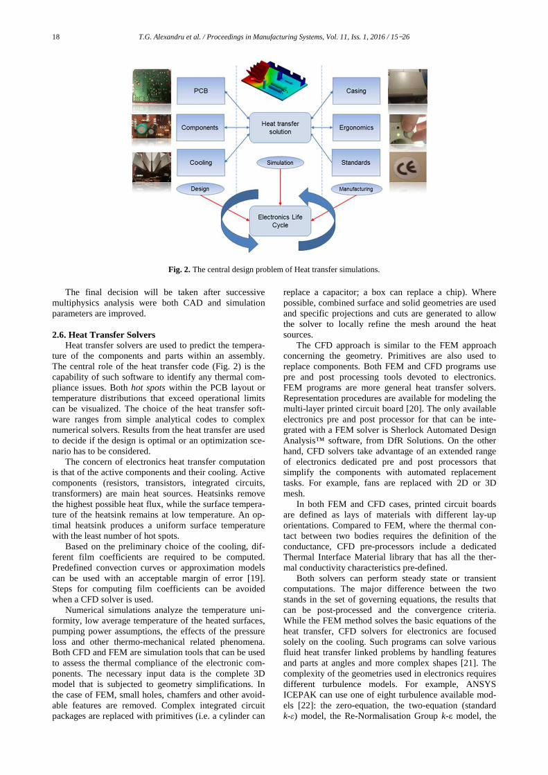
Fig. 13. Post-processed results ‒ temperature and pressure details.

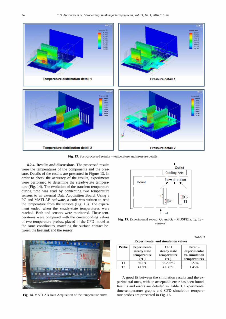
4.2.4. Results and discussions. The processed results were the temperatures of the components and the pres-sure. Details of the results are presented in Figure 13. In order to check the accuracy of the results, experiments were performed to determine the steady-state tempera-ture (Fig. 14). The evolution of the transient temperature during time was read by connecting two temperature sensors to an external Data Acquisition Board. Using a PC and MATLAB software, a code was written to read the temperature from the sensors (Fig. 15). The experi-ment ended when the steady-state temperatures were reached. Both and sensors were monitored. These tem-peratures were compared with the corresponding values of two temperature probes, placed in the CFD model at the same coordinates, matching the surface contact be-tween the heatsink and the sensor.

Fig. 14. MATLAB Data Acquisition of the temperature curve.

Fig. 15. Experimental set-up: Q1 and Q2 ‒ MOSFETs, T1, T2 – sensors.

Table 3

Experimental and simulation values

Probe Experimental steady state temperature

(°C)

CFD steady state temperature

(°C)

Error ‒ experimental vs. simulation temperatures

T1 36.1°C 36.207°C 0.27% T2 41.9°C 41.36°C 1.45%

A good fit between the simulation results and the ex-

perimental ones, with an acceptable error has been found. Results and errors are detailed in Table 3. Experimental time-temperature graphs and CFD simulation tempera-ture probes are presented in Fig. 16.


Fig. 16. Experimental temperature evolution graphs vs. simulation steady-state temperature probes.

5. CONCLUSIONS

Advanced modelling techniques and new simulation strategies were presented for the heat transfer analysis of the electronic components. The multiphysics simulation procedures were employed in conjunction with circuit evaluation software in an original approach. The work-flows ensured efficient model preparation stages and fast verification of the results. The research had an extended literature overview, as well as a large theoretical back-ground. A comparison between Finite Element Method and Computational Fluid Dynamics heat transfer proce-dures was also included.

The thermal management was defined and explained from an integrated PLM point of view, where Electronics Design Automation, Computer Aided Design and Heat Transfer Calculators concepts were developed. The two case studies proved the efficiency and the accuracy of the proposed techniques. Data acquisition tools were used and original MATLAB codes were deployed. Parameters defined and monitored during the experiments were ex-plained and illustrating graphs were provided.

Further work will focus on design optimization based on all simulation strategies discussed, to re-duce expensive material consumption and to find a trade-off between environmental demands, price and product performances, that can be satisfied in respect to the actual standards.

This paper does not only highlight the experimental or simulation procedures, but it is an integrated approach for describing the multiphysics of electronics heat trans-fer.

The novelty of the research consists in the use of in-tegrated simulation tools, tuned with experimental meth-ods that support the workflow.

REFERENCES

[1] Freescale Semiconductor Inc., Thermal Analysis of Semi-conductor Systems, available at: http://cache.nxp.com/files/analog/doc/white_

papep/BasicThermalWP.pdf, accessed: 2016-02-01. [2] W.C. Leong, M.Z. Abdullah, C.Y. Khor and H.J. TAN,

FSI Study of the effect of air inlet/outlet arrangement on the reliability and cooling performances of flexible printed circuit board electronics, Journal of Thermal Science and Technology, Vol. 33, No. 1, 2013, pp. 43‒53.

[3] P. Singhala, D.N. Shah and B. Patel, Temperature Control using Fuzzy Logic, International Journal of Instrumenta-tion and Control Systems (IJICS), Vol. 4, No. 1, 2014, pp. 1‒10.

[4] G. Sharon, Temperature Cycling and Fatigue in Electron-ics, http://www.dfrsolutions.com/wpcontent/up-loads/2014/10/Temperature-CyclingandFatigue-

in-Electronics1.pdf, accessed: 2016-04-01. [5] S. Satyanarayan S., S. Zade, S. Sitre S. and P. Meshram, A

Text Book of Environmental Studies (As per UGC Sylla-bus), Allied Publishers PVT. LTD., New Delhi, 2009.

[6] TÜV Rheinland of North America, Three Challenges Facing the Electronics Industry, available at https://www.tuv.com/media/usa/aboutus_1/pressrelaes/2012_published_articles/quality_dige


st_three_challenges_facing_the_electronics_i

ndustry.pdf, accessed: 2016.02-06. [7] S. Khairnasov and A. Naumova, Heat Pipes Application in

Electronics Thermal Control Systems, Frontiers in Heat Pipes (FHP), Vol. 6, No. 6, 2015, pp.40-54

[8] M. Allsopp, A. Walters, and D. Santillo, Nanotechnologies and nanomaterials in electrical and electronic goods: A review of uses and health concern, Greenpeace Research Laboratories, Technical Note 09/2007, 2007, pp. 1-22.

[9] C. Gargulio, D. Pirozzi, V. Scarano and G. Valentino, A platform to collaborate around CFD simulations, IEEE 23rd International Workshops on Enabling Technologies: Infrastructures for Collaborative Enterprise (WETICE), 2014, pp. 205-210.

[10] J. Li and S. Zhong-Shan, 3D numerical optimization of a heat sink base for electronics cooling, International Com-munications in Heat and Mass Transfer, Vol. 39, No.2, 2012, pp. 204-208.

[11] M. Mazlan, A.F. Zubair, Thermal Management of Elec-tronic Components by Using Computational Fluid Dynam-ics (CFD) Software, FLUENT in Several Material Appli-cations (Epoxy, Composite Material & Nano-silver), Ad-vanced Materials Research, Vol. 795, 2013, pp. 141‒ 147.

[12] B. Ramos-Alvarado, H. Liu and A. Hernandez-Guerrero, CFD Study of liquid-cooled heat sinks with microchannel flow field configurations for electronics, fuel cells and concentrated solar cells, Applied Thermal Engineering, Vol. 31, No. 14, pp. 2494‒2507.

[13] J.N. Davidson, D.A. Stone, M.P. Foster and D.T. Gladwin, Real - Time Temperature Estimation in a Multiple Device Power Electronics System Subjected to Dynamic Cooling, IEEE Transactions in Power Electronics, Vol. 31, No. 4, 2016, pp. 2709‒2719.

[14] Ellison G.N., Thermal Computations for Electronics Con-ductive, Radiative and Convective Air Cooling, CRC Press Taylor & Francis Group, New York, 2011.

[15] ANSYS Inc., Thermal Analysis Guide, Release 12.0, April 2009.

[16] LUSAS Inc., Modeler Reference Manual LUSAS Version 14.5 : Issue 1, available at: http://www.lusas.cn-/protected/documentation/V14_5/Modeller%20Re

ference%20Manual.pdf, accessed: 2016-02-05. [17] A. Sayma, Computational Fluid Dynamics, Ventus Pub-

lishing, 2009. [18] Morgan Advanced Materials, Web Based Heat Transfer

Calculator, available at http://morganhea-

tflow.com/Account/Login?ReturnUrl=%2f, ac-cessed: 2016-01-15.

[19] K. Lawrence K., ANSYS Workbench Tutorial, Schroff Development Corporation, United States of America, 2005.

[20] S. Rzepka, F. Krämer, O. Grassmé, and J. Lienig, A multi-layer PCB material modeling approach based on laminate theory, Thermal, Mechanical and Multi-Physics Simula-tion and Experiments in Microelectronics and Micro-Systems, edited by G.Q. Zhang, Freiburg-im-Breisgau, Germany, April 2008, pp. 234‒243.

[21] V.H. Wong, FloTHERM XT Introduction FloTHERM v10 demonstration, available at http://www.flotre-nd.com.tw/news_center/epaper/2013/06/data/Fl

oTHERM_XT_0523.pdf, accessed: 2016-02-10. [22] ANSYS INC, ANSYS ICEPAK 14.0 Documentation, 2011. [23] P.W. Ross, The Handbook of Software for Engineers and

Scientists, CRC Press, 1995. [24] ANSYS INC, ANSYS FLUENT Theory Guide 16.1 Docu-

mentation, April 2015. [25] G.K. Batchelor, An Introduction to Fluid Dynamics. Cam-

bridge Univ. Press. Cambridge, UK. 1967, pp. 726. [26] S.T. Microelectronics, IRF630 N-channel 200 V, 0.35

Ohm typ., 9 A Power MOSFET in D2PAK package, avail-able at http://www.st.com/st-web-/technical/doc ument/datasheet/CD00000701.pd,access.2016.02.10.

heat transfer simulation for thermal management of electronic...

Documents