heat transfer to and from a reversible thermosiphon placed
TRANSCRIPT
HEAT TRANSFER TO AND FROM A REVERSIBLE THERMOSIPHON
PLACED IN POROUS MEDIA
by
Bidzina Kekelia
A dissertation submitted to the faculty of The University of Utah
in partial fulfillment of the requirements for the degree of
Doctor of Philosophy
Department of Mechanical Engineering
The University of Utah
May 2012

Copyright © Bidzina Kekelia 2012
All Rights Reserved

T h e U n i ve r s i t y o f U ta h Gr ad u a t e S c h oo l
STATEMENT OF DISSERTATION APPROVAL
The dissertation of Bidzina Kekelia
has been approved by the following supervisory committee members:
Kent S. Udell , Chair October 18, 2011
Date Approved
Timothy A. Ameel , Member November 2, 2011
Date Approved
Kuan Chen , Member October 18, 2011
Date Approved
Meredith M. Metzger , Member October 19, 2011
Date Approved
Milind Deo , Member October 31, 2011
Date Approved
and by Timothy A. Ameel , Chair of
the Department of Mechanical Engineering
and by Charles A. Wight, Dean of The Graduate School.

ABSTRACT
The primary focus of this work is an assessment of heat transfer to and from a reversible
thermosiphon imbedded in porous media. The interest in this study is the improvement of
underground thermal energy storage (UTES) system performance with an innovative ground
coupling using an array of reversible (pump-assisted) thermosiphons for air conditioning or space
cooling applications. The dominant mechanisms, including the potential for heat transfer
enhancement due to natural convection, of seasonal storage of “cold” in water-saturated porous
media is evaluated experimentally and numerically. Winter and summer modes of operation are
studied.
A set of 6 experiments are reported that describe the heat transfer in both fine and
coarse sand in a 0.32 cubic meter circular tank, saturated with water, under freezing (due to heat
extraction) and thawing (due to heat injection) conditions, driven by the heat transfer to or from
the vertical thermosiphon in the center of the tank. It was found that moderate to strong natural
convection was induced at Rayleigh numbers of 30 or higher. Also, near water freezing
temperatures (0°C-10°C), due to higher viscosity of water at lower temperatures, almost no
natural convection was observed.
A commercial heat transfer code, ANSYS FLUENT, was used to simulate both the
heating and cooling conditions, including liquid/solid phase change. The numerical simulations of
heat extraction from different permeability and temperature water-saturated porous media
showed that enhancement to heat transfer by convection becomes significant only under
conditions where the Rayleigh number is in the range of 100 or above. Those conditions would be
found only for heat storage applications with higher temperatures of water (thus, its lower
viscosity) and large temperature gradients at the beginning of heat injection (or removal) into
(from) soil. For “cold” storage applications, the contribution of natural convection to heat transfer

iv
in water-saturated soils would be negligible. Thus, the dominant heat transfer mechanism for air
conditioning applications of UTES can be assumed to be conduction.
An evaluation of the potential for heat transfer enhancement in air-saturated media is
also reported. It was found that natural convection in soils with high permeability and air
saturations near 1 becomes more important as temperatures drop significantly below freezing.
TABLE OF CONTENTS
ABSTRACT ...................................................................................................................................... iii
LIST OF FIGURES ........................................................................................................................ viii
LIST OF TABLES .......................................................................................................................... xiii
NOMENCLATURE......................................................................................................................... xiv
ACKNOWLEDGMENTS ................................................................................................................ xvi
1. INTRODUCTION ....................................................................................................................... 1
Current Thermal Energy Storage Technologies ...................................................................... 2 Soil for Energy Storage ........................................................................................................... 4 Ground Source Heat Pumps ................................................................................................... 5 Ground Coupling Methods – In-Ground Heat Exchangers ..................................................... 5 Thermosiphon as a Ground Coupling Device ......................................................................... 6 Reversible Thermosiphon........................................................................................................ 7 Air Conditioning or Space Cooling Potential ......................................................................... 10 References ............................................................................................................................ 13
2. PROBLEM FORMULATION AND METHODS........................................................................ 17
Heat Transfer Domain ........................................................................................................... 17 Theoretical Model .................................................................................................................. 18 Maximum Fluid Velocity During Natural Convection in Porous Medium ............................... 24 Methods for Estimating Heat Transfer Rates to/from Porous Medium ................................. 26 Selection of Porous Media for the Experiments .................................................................... 31 References ............................................................................................................................ 35
3. PROPERTIES OF POROUS MEDIA ...................................................................................... 36
Porosity and Permeability ...................................................................................................... 36 Sand Properties ..................................................................................................................... 42 Water Properties .................................................................................................................... 44 Ice Properties ........................................................................................................................ 48 Conduction Models for Porous Media ................................................................................... 54 Verification of Selected Conduction Model ............................................................................ 59 References ............................................................................................................................ 65
4. EXPERIMENTAL SETUP AND PROCEDURES .................................................................... 67
Experimental Apparatus ........................................................................................................ 67 Experimental Procedures ...................................................................................................... 70 References ............................................................................................................................ 72
vi
5. EXPERIMENTAL RESULTS ................................................................................................... 73
Uncertainty Analysis .............................................................................................................. 73 Rayleigh Numbers and Temperature Distribution in Porous Media during Heat Extraction . 92 Rayleigh Numbers and Temperature Distribution in Porous Media during Heat Injection .. 111 Heat Transfer Rates during Heat Extraction from Water-Saturated Porous Media ............ 118 Heat Transfer Rates during Heat Injection into Water-Saturated Porous Media ................ 133 Thermosiphon Performance ................................................................................................ 134 References .......................................................................................................................... 137
6. NUMERICAL SIMULATIONS ............................................................................................... 139
Software Limitations and Simplifications ............................................................................. 139 Domain and Setup for Simulations ...................................................................................... 142 Results of Simulation of the Heat Extraction Experiment with a Transient Temperature Boundary Condition ............................................................................................................. 145 Results of Simulations with Constant Temperature Boundary Conditions and Different Permeabilities and Initial Temperatures .............................................................................. 150 References .......................................................................................................................... 156
7. GRID-INDEPENDENT AIR CONDITIONING USING UNDERGROUND THERMAL ENERGY STORAGE (UTES) AND REVERSIBLE THERMOSIPHON TECHNOLOGY – EXPERIMENTAL RESULTS ................................................................................................. 157
Abstract................................................................................................................................ 158 Introduction .......................................................................................................................... 158 Nomenclature ...................................................................................................................... 158 Underground Thermal Energy Storage ............................................................................... 159 Ground Source Heat Pumps and Ground Coupling Methods ............................................. 159 Reversible Thermosiphon.................................................................................................... 159 Grid-Independent Air Conditioning System ......................................................................... 160 Lab-Scale Prototype ............................................................................................................ 160 Experimental Results and Discussion ................................................................................. 160 Conclusions ......................................................................................................................... 166 References .......................................................................................................................... 166
8. ENERGY STORAGE IN DRY SOILS: RAYLEIGH NUMBERS FOR AIR-SATURATED VS. WATER-SATURATED POROUS MEDIA ............................................................................. 168
References .......................................................................................................................... 176
9. DISCUSSION AND CONCLUSIONS .................................................................................... 177
APPENDICES
A - MATLAB CODE FOR FITTING POLYNOMIAL FUNCTIONS TO SAND (QUARTZ) PROPERTIES .............................................................................................................................. 179
B - MATLAB CODE FOR FITTING POLYNOMIAL FUNCTIONS TO WATER PROPERTIES .. 183
C - MATLAB CODE FOR FITTING POLYNOMIAL FUNCTIONS TO ICE PROPERTIES ......... 187
D - DERIVATION OF MAXWELL’S EQUATION FOR CONDUCTIVITY OF POROUS MEDIA . 189
E - MATLAB CODE FOR THERMAL CONDUCTIVITY MODELS FOR POROUS MEDIA ........ 191

vii
F - USER-DEFINED FUNCTION (UDF) FOR TRANSIENT TEMPERATURE BOUNDARY CONDITION FOR FLUENT ......................................................................................................... 194
G - MATLAB CODE FOR RAYLEIGH NUMBERS FOR AIR-SATURATED VS. WATER-SATURATED POROUS MEDIUM............................................................................................... 195

LIST OF FIGURES
Figure Page
1.1: Tank storage: (a) 50,000 m3 hot water, Theiß district heating plant in Gedersdorf, Austria,
(b) 150 m3 hot water, greenhouse in Nürnberg, Germany, (c) hot water, district heating plant in
Chemnitz, Germany. ........................................................................................................................ 3
1.2: Thermosiphons installed on the Trans-Alaska Pipeline between Fort Greeley and Black Rapids, Alaska, a region with discontinuous permafrost. ................................................................ 8
1.3: Thermosiphon operation in passive mode – heat extraction. .................................................. 9
1.4: Reversible thermosiphon operation – heat injection. ............................................................ 10
1.5: Array of thermosiphons. ........................................................................................................ 11
2.1: Top view of an internal thermosiphon cell in an array of thermosiphons. Also shown is an equivalent circular boundary that would approximate an actual hexagon. ................................... 18
2.2: Heat injection in the soil for a cylindrical cell (vertical cross-section). ................................... 19
2.3: Vertical cross-section of a cylindrical cell of the porous medium with a thermosiphon. The volume is divided into a large number of small (elemental) concentric rings. ............................... 27
2.4: Orifice meter schematics for air flow measurements ............................................................ 29
2.5: Calculated Rayleigh numbers and permeabilities of water-saturated porous media for different mean diameters of sand particles ( = 40%, = 1, = 10). ............................... 33
3.1: Illustration of Darcy's Law. ..................................................................................................... 37
3.2: Constant head permeameter for determining soil permeability in the lab environment: (a) simple permeameter with constant head, (b) filter paper and narrow inlet/outlet passage valves adding resistance to water flow. .................................................................................................... 39
3.3: Redesigned permeameter: (a) doubled cylinder length, (b) increased inlet/outlet diameter and no valves are shown, (c) filter paper was replaced with aluminum mesh, (d) redesigned permeameter positioned horizontally. ........................................................................................... 40
3.4: Specific heat capacity of quartz. ............................................................................................ 42
3.5: Thermal conductivity of quartz............................................................................................... 43
3.6: Water density variation with temperature. ............................................................................. 45
3.7: Water specific heat capacity variation with temperature. ...................................................... 46

ix
3.8: Water dynamic (absolute) viscosity variation with temperature. ........................................... 47
3.9: Water thermal conductivity variation with temperature. ........................................................ 49
3.10: Water thermal expansion coefficient variation with temperature. ........................................ 50
3.11: Ice density variation with temperature. ................................................................................ 51
3.12: Ice specific heat capacity variation with temperature. ......................................................... 52
3.13: Ice thermal conductivity variation with temperature. ........................................................... 53
3.14: Conduction models: (a) series, (b) parallel and (c) 3-element resistor (conductor) [10, 11]. ....................................................................................................................................................... 55
3.15: Thermal conductivity models for porous media (water-saturated sand at 20°C). ............... 56
3.16: Heat injection time-profile in undisturbed porous media for measurement of its thermal conductivity. ................................................................................................................................... 60
3.17: Thermal conductivity measurements of water-saturated fine sand (Mar 26-27, 2011). Each line represents a separate experiment. Experiments with the same heat injection times have the same color. ..................................................................................................................... 62
3.18: Thermal conductivity measurements of water-saturated coarse sand (Mar 24-25, 2011). Each line represents a separate experiment. Experiments with the same heat injection times have the same color. ..................................................................................................................... 63
3.19: Experimental setup for thermal conductivity measurements of water-saturated sand: (a) centrally positioned heating cartridge and type-T thermocouple, (b) coarse sand and data logger. ............................................................................................................................................ 64
4.1: Experimental apparatus: (a) thermocouple array attached to thermosiphon wall, (b) thermosiphon inside a thermally insulated tank filled with water-saturated sand. ........................ 68
4.2: Experimental apparatus - assembly details: (a) pump and filter assembly, (b) aluminum screen/mesh, (c) thermocouple array. ........................................................................................... 69
4.3: Experimental apparatus - orifice flow meter details on the air duct: (a) orifice and pressure outlet locations, (b) U-tube manometer filled with water. .............................................................. 70
5.1: Relative uncertainties in thermal conductivities of water-saturated fine and coarse sand packs. ............................................................................................................................................ 83
5.2: Relative uncertainties in volumetric heat capacity of water-saturated fine and coarse sand packs. ............................................................................................................................................ 85
5.3: Uncertainty in thermal expansion coefficient of water. .......................................................... 88
5.4: Thermal expansion coefficient of water in 0°C-20°C temperature range. ............................. 89
5.5: Uncertainty in Rayleigh numbers for = − ∞ = 5&20. ...................................... 92
5.6: Temperature dependence of Rayleigh numbers and associated uncertainties for = − ∞ = 5&20 for the water-saturated fine sand pack. ................................................... 93

x
5.7: Temperature dependence of Rayleigh numbers and associated uncertainties for = − ∞ = 5&20 for the water-saturated coarse sand pack. .............................................. 94
5.8: Temperatures during heat removal from fine sand pack on Dec 4-12, 2009. ....................... 97
5.9: Temperatures during heat removal from fine sand on Dec 26, 2009 - Jan 2, 2010.............. 98
5.10: Temperatures during heat removal from coarse sand pack on Feb 7-14, 2010. ................ 99
5.11: Temperatures during heat removal from coarse sand pack on Feb 19-25, 2010. ............ 100
5.12: Characteristic isotherms during heat removal from fine sand pack on Dec 4-12, 2009 at 0.5 h, 36 h and 150 h from the beginning of the experiment. .................................................. 102
5.13: Characteristic isotherms during heat removal from fine sand pack on Dec 26, 2009 - Jan 2, 2010 at 0.5 h, 36 h and 62 h from the beginning of the experiment. ................................ 103
5.14: Characteristic isotherms during heat removal from coarse sand pack on Feb 7-14, 2010 at 0.5 h, 24 h and 50 h from the beginning of the experiment. .................................................... 104
5.15: Characteristic isotherms during heat removal from coarse sand pack on Feb 19-25, 2010 at 0.5 h, 9 h and 48 h from the beginning of the experiment. ............................................. 105
5.16: Ra numbers during heat removal from fine sand pack on Dec 4-12, 2009. ...................... 106
5.17: Ra numbers during heat removal from fine sand pack on Dec 26, 2009 - Jan 2, 2010. ... 107
5.18: Ra numbers during heat removal from coarse sand pack on Feb 7-14, 2010. ................. 108
5.19: Ra numbers during heat removal from coarse sand pack on Feb 19-25, 2010. ............... 109
5.20: Temperatures during heat injection in fine sand pack on Jan 2-4, 2010. ......................... 112
5.21: Temperatures during heat injection in coarse sand pack on Feb 25-27, 2010. ................ 113
5.22: Characteristic isotherms during heat injection in fine sand pack on Jan 2-4, 2010 at 1 h, 24 h and 40 h from the beginning of the experiment. .................................................................. 114
5.23: Characteristic isotherms during heat injection in coarse sand pack on Feb 25-27, 2010 at 1 h, 24 h and 40 h from the beginning of the experiment. ....................................................... 115
5.24: Ra numbers during heat injection in fine sand pack on Jan 2-4, 2010. ............................ 116
5.25: Ra numbers during heat injection in coarse sand pack on Feb 25-27, 2010. ................... 117
5.26: Heat extraction rates from fine sand pack during the Dec 4-12, 2009 experiment: (a) heat transfer rates, (b) inlet and outlet air temperatures in the heat exchanger. ........................ 119
5.27: Heat extraction rates from fine sand pack during the Dec 26, 2009 – Jan 2, 2010 experiment: (a) heat transfer rates, (b) inlet and outlet air temperatures in the heat exchanger. 120
5.28: Heat extraction rates from coarse sand pack during the Feb 7-14, 2010 experiment: (a) heat transfer rates, (b) inlet and outlet air temperatures in the heat exchanger. ........................ 121
xi
5.29: Heat extraction rates from coarse sand pack during the Feb 19-25, 2010 experiment: (a) heat transfer rates, (b) inlet and outlet air temperatures in the heat exchanger. ................... 122
5.30: Heat injection rates into fine sand pack during the Jan 2-4, 2010 experiment: (a) heat transfer rates, (b) inlet and outlet air temperatures in the heat exchanger. ................................ 123
5.31: Heat injection rates into coarse sand pack during the Feb 25-27, 2010 experiment: (a) heat transfer rates, (b) inlet and outlet air temperatures in the heat exchanger. ........................ 124
5.32: Cumulative heat extracted from fine sand pack during the Dec 4-12, 2009 experiment. . 125
5.33: Cumulative heat extracted from fine sand pack during the Dec 26, 2009 – Jan 2, 2010 experiment. .................................................................................................................................. 126
5.34: Cumulative heat extracted from coarse sand pack during the Feb 7-14, 2010 experiment. .................................................................................................................................. 127
5.35: Cumulative heat extracted from coarse sand pack during the Feb 19-25, 2010 experiment. .................................................................................................................................. 128
5.36: Cumulative heat injected into fine sand pack during the Jan 2-4, 2010 experiment. ........ 129
5.37: Cumulative heat injected into coarse sand pack during the Feb 25-27, 2010 experiment. .................................................................................................................................. 130
5.38: Uniform ice build-up during heat extraction experiment on Jan 21-30, 2009. ................... 135
5.39: Temperatures on outer surface of the thermosiphon during heat removal experiment from fine sand pack on Dec 4-12, 2009. ..................................................................................... 135
6.1: Application of the thermal conductivity model used in ANSYS FLUENT for water- saturated sand pack. ................................................................................................................... 141
6.2: Face of axi-symmetric cylindrical domain. ........................................................................... 143
6.3: Fitted polynomial function of T(K) vs. t(sec) for the thermosiphon wall. ............................. 144
6.4: Isotherms after 30 h (1800 min): (a) experimental data and (b) simulations for the same conditions and geometry. ............................................................................................................ 146
6.5: Simulation results: (a) freezing front and (b) stream functions after 30 h (1800 min). ........ 147
6.6: Simulation results: (a) velocity magnitudes and (b) vectors after 30 h (1800 min). ............ 148
6.7: Simulation results: (a) velocity vectors and (b) isotherms after 20 h................................... 149
6.8: Maximum fluid velocities during heat extraction simulations from water-saturated porous media (sand packs). .................................................................................................................... 151
6.9: Rayleigh numbers during heat extraction simulations from water-saturated porous media (sand packs). ............................................................................................................................... 152
6.10: Dependence of maximum fluid velocities on Rayleigh number. ........................................ 153

xii
6.11: Heat transfer rates during heat extraction simulations from water-saturated porous media (sand packs). .................................................................................................................... 154
7.1: Passive soil precooling (heat extraction). ............................................................................ 159
7.2: Air conditioning mode (heat injection). ................................................................................ 160
7.3: (a) Lab-scale reversible thermosiphon prototype with attached thermocouple array, data logger and heat exchanger, (b) thermosiphon inserted into a thermally insulated tank with water-saturated sand pack. ......................................................................................................... 160
7.4: Heat extraction rate from fine sand. .................................................................................... 161
7.5: Heat extraction rate from coarse sand. ............................................................................... 161
7.6: Heat injection rate in coarse sand. ...................................................................................... 161
7.7: Isotherms of freezing fine sand after 1 h. ............................................................................ 162
7.8: Isotherms of freezing fine sand after 10 h. .......................................................................... 162
7.9: Isotherms of freezing fine sand after 94 h. .......................................................................... 163
7.10: Isotherms of cooling coarse sand after 1 h. ...................................................................... 163
7.11: Isotherms of cooling coarse sand after 10 h. .................................................................... 163
7.12: Isotherms of cooling coarse sand after 40 h. .................................................................... 164
7.13: Isotherms of heat injection in fine sand after 1 h. .............................................................. 164
7.14: Isotherms of heat injection in fine sand after 10 h. ............................................................ 164
7.15: Isotherms of heat injection in fine sand after 24 h. ............................................................ 165
7.16: Isotherms of heat injection in coarse sand after 1 h. ......................................................... 165
7.17: Isotherms of heat injection in coarse sand after 10 h. ....................................................... 165
7.18: Isotherms of heat injection in coarse sand after 24 h. ....................................................... 166
8.1: Kinematic viscosities of water and air [3, 4]. ....................................................................... 169
8.2: Thermal expansion coefficients for water and air [3, 4]. ...................................................... 170
8.3: Thermal conductivities of PM with = 40%, saturated with water, ice or air. .................... 171
8.4: Volumetric heat capacity of PM with = 40%, saturated with water, ice or air. ................. 172
8.5: Thermal diffusivities of PM with = 40%, saturated with water, ice or air. ........................ 173
8.6: Ra numbers for water- vs. air-saturated porous medium .................................................... 175

LIST OF TABLES
Table Page
3.1: Variation of sand properties with temperature........................................................................ 45
3.2: Variation of water properties with temperature....................................................................... 47
3.3: Variation of ice properties with temperature. .......................................................................... 53
5.1: Summary of data on characteristic experiments. .................................................................. 74
5.2: Permeability measurement results for coarse and fine sand packs. ..................................... 79
5.3: Summary of uncertainties. ..................................................................................................... 95

NOMENCLATURE
coefficient defined on page 64
area [m2]
coefficient defined on page 64
specific heat [J/kg·K] or coefficient defined
on page 64 overall orifice loss coefficient
average sand grain diameter [m] or
coefficient defined on page 64 orifice or duct diameter
Fourier number (non-dimensional time)
gravitational acceleration [m/s2] or particle
shape factor ℎ enthalpy [J/kg] or height [m]
ℎ latent heat of fusion [J/kg]
permeability [m2]
hydraulic conductivity [m/s]
! weighting factor of distribution of phases in
the porous medium " pressure [N/m2]
# Darcy’s velocity [m/s]
#" heat flux [W/m2]
% volumetric flow rate [m3/s]
%& heat transfer rate [W]
' horizontal (radial) coordinate [m]
( electrical resistance [Ohm]
() Reynolds number, () = *+,
- time [s]
temperature [K or °C]
. velocity [m/s] or relative uncertainty [%]
/ uncertainty
0 volume [m3] or voltage [V]
1 vertical coordinate [m]

xv
Greek symbols 2 thermal diffusivity [m2/s]
3 thermal expansion coefficient [1/K] or ratio
of the orifice diameter to the diameter of
the duct 4 fraction of liquid in fluid
5 fraction of liquid in volume element
6 thermal conductivity [W/m·K]
7 dynamic viscosity [N·s/m2]
8 kinematic viscosity [m2/s]
9 density [kg/m3]
: standard deviation
porosity
; pressure potential [Pa]
< stream function
= ratio of fluid volumetric heat capacity to
fluid-filled porous medium volumetric heat
capacity
Subscripts air
cross section
'- heating cartridge
)>> effective
> fluid
? ice or initial
@ liquid
porous matrix or mean
A point of maximum density
orifice or reference state
B pore, constant pressure or parallel
B porous medium
' radial direction
sand, solid, surface or serial
C constant volume
D water
1 vertical direction
∞ far field

ACKNOWLEDGMENTS
I would like to express my gratitude to my adviser, Dr. Kent S. Udell, who has introduced
me to the field of multiphase transport in porous media and has been guiding my research during
my studies at the University of Utah. I would like to thank him for all his efforts and support he has
provided me and my family during the difficult times of political instability in my home country and
during my stay in the United States.
I would like to thank members of my graduate committee for their direction and
suggestions. I very much value the knowledge I have acquired from them during classroom
instruction as most of them have been my lecturers in several subjects.
I would like to acknowledge the support of the Department of Mechanical Engineering of
the University of Utah which provided much needed assistance for continuation of my research
and completion of my studies.

1. INTRODUCTION
A high proportion of our energy consumption is in the form of low-grade heat at
temperatures less than 100°C. In the US, according to the U.S. Energy Information
Administration, 41% of the total energy consumption is for residential and commercial sectors'
energy needs, with over a third used for space/water heating and air conditioning [1]. It is a waste
of exergy to use high-grade electricity or to burn oil, gas or coal at temperatures of up to 1000°C
in order to create an indoor climate at 20-25°C. With the depletion of fossil fuel reserves and
increasing global temperatures due to greenhouse gas emissions from burning them, the notion
of long-term thermal energy storage, which can store low-cost, often free, low-grade energy to be
used at any time at our discretion, becomes more and more appealing. In addition to energy
savings, energy independence and security is becoming increasingly important and seasonal
storage of energy provides a feasible means to achieve them.
Thermal energy storage can be a relatively cheap or sometimes free energy source (or
cold sink) completely satisfying our requirements for space and water heating or air conditioning
year-round. Storing excess heat in summer for future winter use and winter “cold” for summer air
conditioning can provide space heating and cooling with negligible or even no fossil fuel use.
Large size storage can help in reducing loads on the power system, especially in peak heating or
air conditioning periods, eliminating the need for new (most probably fossil fueled) power plants.
In case there is still a need for additional power purchases, it can shift those to low-cost (off-peak)
periods. One principle gain from thermal storage is that it allows utilization of thermal energy or
“cold” that would otherwise be lost because it was available only at a time of no demand.
Therefore, seasonal thermal energy storage makes possible the effective utilization of sources
like solar energy, process waste heat or ambient heat/cold.

2
Current Thermal Energy Storage Technologies
There are numerous variations of thermal energy storage systems reviewed in the
literature [2-4]. Some most common ones are listed below:
• Underground or above-ground tank storage with stratified liquid (Figure 1.1)
• Lakes and solar ponds with high salinity gradient [5-8]
• Encapsulated or bulk phase-change materials (ice or various salts) in storage tanks [9]
• Thermo-chemical reactions in storage tanks [4]
• Earth pits for sensible heat storage with concrete walls and bottom [4]
• Underground rock caverns for storing high temperature water under high pressure [4]
• Storage using underground aquifer water (vertical boreholes with open pipe loop) [4]
• Underground storage directly in soil (with horizontal air ducts/coils or vertical boreholes
with closed pipe loops) [4, 10]
• Hybrid systems – underground water tank surrounded by boreholes in the soil [11, 12]
Each of the above-listed technologies has its advantages and drawbacks, specific to
design requirements and local conditions. Storage systems based on thermo-chemical reactions
have negligible heat losses whereas phase-change materials (PCM) and especially sensible heat
storage dissipate the stored heat to the surroundings. Even though PCMs and thermo-chemical
reactants possess higher energy densities, their cost, lower heat transfer coefficients (compared
to stratified fluid tanks), corrosion problems and toxicity (except when ice is used) restrict their
applicability. Sensible heat storage has the advantage of being cheap, but due to its relatively low
energy density, large volumes are typically required.
In most cases of thermal energy storage, a large tank/reservoir is used, which is costly to
build/manufacture, or a suitable lake, underground aquifer or underground rock cavern has to
exist on the project site. The proposed reversible thermosiphon-assisted storage (described in the
following chapters) allows thermal energy storage directly in soil and does not require any storage
reservoir, similar to ground source heat pump (GSHP) technology, but operates without vapor
compression cycle refrigeration equipment and large circulation pumps needed for a GSHP
system.

3
(a)
(c)
(b)
Figure 1.1: Tank storage: (a) 50,000 m3 hot water, Theiß district heating plant in Gedersdorf,
Austria,1 (b) 150 m
3 hot water, greenhouse in Nürnberg, Germany,
2 (c) hot water, district heating
plant in Chemnitz, Germany.3
1 Image source: www.wikipedia.org Author: Ulrichulrich. License: Public domain.
2 Image source: www.wikipedia.org Author: AphexTwin. License: Public domain.
3 Image source: www.wikipedia.org Author: Kolossos. License: Public domain.

4
Soil for Energy Storage
The large thermal storage capacity of the earth provides a very attractive source of heat
or cold storage which can be utilized for a variety of purposes. The idea of thermal energy
storage in soil is not new. The first patent on the use of the ground as a heat sink was issued in
Switzerland in 1912 to Swiss engineer and inventor Heinrich Zoelly4 [13, 14, 15]. If soil is used as
the energy storage medium, there is no restriction on the storage volume other than the potential
constraint of keeping near-surface ground temperatures close to their natural values to avoid
unwanted impact on surface soil flora and fauna. If heated and cooled in an optimum way, soil
can provide not only a buffer for short-term fluctuations in supply and demand, but can
accommodate a complete annual heating/cooling load and serve a seasonal balancing function
[16-26]. Energy storage directly in soil also reduces the cost sensitivity of reservoir sizing for
optimum capacity selection. So, in most cases, if the storage size is restricted on the surface, it
can be easily sized to a maximum expected load by a simple increase of depth. Energy recovery
efficiency for already implemented underground thermal energy storages (UTES) encountered in
the literature [18] ranges from 47% to 73%.
The main advantages of using native soil are:
• It is inexpensive (does not require reservoirs),
• It has sufficient thermal capacity and relatively low conductivity (lowering ambient heat
losses),
• It has almost no size/volume restrictions (thus, its low energy density is not an issue),
• It is universally available.
Furthermore, in climates where the temperatures in the winter drop below freezing for
significant periods of time, the effective heat capacity of soil increases substantially due to the
latent heat of freezing/melting of water within the soil.
4 Heinrich Zoelly (1862-1937), well known Swiss engineer, graduate of Zurich Polytechnicum, better known for his
inventions and patent (1903) on impulse steam turbine.

5
Ground Source Heat Pumps
Ground source heat pumps are the most commonly used technology for utilization of soil
for underground thermal energy storage systems [13-15, 26]. An estimated 1.1 million systems
have been installed worldwide [27]. GSHPs use vapor compression cycle refrigeration equipment,
intermediary heat exchangers and additional circulation pumps for pumping an intermediate
working fluid (water glycol solution) in underground plastic piping or raising water from aquifer
wells, thus adding equipment and operational costs to the system. Besides, as significant energy
(electricity) input is required for the GSHP system to operate, its coefficient of performance (COP)
rarely exceeds COPHP = 4 [28].
Ground Coupling Methods – In-Ground Heat Exchangers
The major problem associated with using the ground as a storage medium is in finding an
efficient method of extracting or injecting heat. Generally, this is achieved through PVC or
polyethylene pipe loops installed horizontally or in vertical U-shaped loops in the boreholes,
serving as heat exchangers with soil. Plastics are used for economic reasons; however, they
have a low thermal conductivity, typically an order of magnitude less (0.10-0.25 W/m·K) than that
of soil (0.84-3.0 W/m·K), hindering heat exchange with the ground [29]. Besides, in vertical
boreholes, there is a thermal penalty due to the proximity of counterflowing hot and cold working
fluid streams in the U-loop which exchange heat with each other [30]. This, of course, increases
the total borehole length required for a given thermal load of the system.
A relatively new concept of burying plastic pipes in the ground using a “no-dig method”
developed at the University of Hokkaido, Japan, is reviewed in [31]. The method uses a self-
propelled flexible drill-head which pulls the plastic heat exchanger piping behind as it drills
spiraling loops into the ground. This technique avoids the thermal penalty of vertical borehole U-
loops, mentioned in the previous paragraph, and the higher heat losses of horizontal heat
exchangers installed close to the ground surface, but requires the use of expensive equipment
and has not found a widespread application.
Some building cooling designs have used air ducts as heat exchangers with the ground,
but stagnant water in the passages caused by ground water infiltration or humidity condensation
6
from the air have lead to sanitary problems. Direct space cooling with earth-to-water and then
water-to-air heat exchange without a heat pump has been experimentally studied in Italy [32], but
the system required a large amount of circulating pumping power to pump the water through the
underground piping.
Another interesting technology, often referred to as “direct-exchange”, uses copper pipes
as in-ground heat exchangers with refrigerating agent flowing directly in those pipes. This
eliminates the intermediary working fluid (water glycol solution), plastic piping, intermediary water-
to-refrigerant heat exchanger and circulating pump, and increases effectiveness of heat transfer
with the soil [33-35]. Aside from copper piping cost and potential refrigerant leaks in the ground,
this is an improvement over traditional GSHP technology; however, a direct-exchange heat pump
still requires vapor compression equipment and significant electric power.
Even though new methods of installing heat exchangers in the ground are being
developed to simplify their installation, the above-mentioned ground coupling schemes still
employ vapor compression-based heat pumps or water circulating pumps which need large
external power input, thereby reducing their COP.
Thermosiphon as a Ground Coupling Device
In contrast to GSHPs, a system which is based on an innovative new concept of using
reversible thermosiphons as the means of ground coupling [36, 37] can achieve a very high, if not
infinite (in case of passive operation), coefficient of performance as there is very little or no
energy input needed for pumping heat (“cold”) from/to soil.5 Due to much more effective latent
heat capture/release phenomena, characteristic of heat pipes and thermosiphons, even a small
(few degrees) temperature gradient between the storage medium and heated (cooled) air is a
sufficient driving mechanism for moving heat from (to) soil.
Thermosiphons are a variation of heat pipes, in which a working fluid circulates under the
force of gravity instead of capillary forces of wicking materials used in heat pipes. The first patent
5 This is true for air conditioning applications when soil temperatures are lower than that of cooled air temperature and
suitable for direct heat exchange with air. If UTES is used for space or water heating purposes, the soil temperature has to be either preraised up to 70-90°C by solar or other heat injection [9] or additional heat pump employed for further raising working fluid temperature to above room temperatures. In the latter case, additional energy input will be required which will decrease the COPHP, but is still expected to be higher than that of traditional GSHP COPs.
7
application for a heat pipe concept belongs to R.S. Gaugler of the General Motors Corporation,
Ohio, USA and is dated December 21st, 1942 [38, 39]. The term “heat pipe” was used only later,
in G.M. Grover’s 1963 patent application [40] and his paper published in 1964 [41]. Due to very
high heat transfer capabilities, light weight, no moving parts (i.e. high reliability) and ability to
operate in zero gravity, heat pipes received significant attention and boost in development as
satellite and spacecraft thermal management devices in the late 60s and 70s. Space applications
were followed by numerous terrestrial designs ranging from small electronic device coolers [42] to
large industrial heat exchangers, underground supports of various structures to keep permafrost
from melting [43], to applications for melting snow on roads, pavements and railway tracks [44,
46], and evacuated hot water solar collectors. Heat pipes were successfully used on marine
vessels operating in arctic waters for deicing decks [45]. They have been used in cooling system
designs for thermal [46] and even nuclear power plants for removal of residual heat released in
the reactor core in case of an accident and interruption of coolant water supply by primary pumps
[43].
Passive, nonreversible thermosiphons have been successfully used as ground coupling
devices in winter heating applications to keep greenhouse temperatures above freezing in
Belarus [47, 48, 49] and with a heat pump booster for space heating in Austria [50, 51]. The
working fluid used in the thermosiphons in Belarus was ammonia (NH3) and carbon dioxide (CO2)
was used in Austria. Thermosiphon application has been suggested in Italy for extracting heat
from low enthalpy geothermal reservoirs (hot water aquifers with relatively low temperatures not
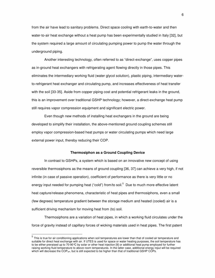
capable of developing steam) close to the ground surface [52]. The most well-known large-scale
application of thermosiphons, with over 100,000 installed (Figure 1.2) and ammonia as the
working fluid, is in the Trans-Alaskan oil pipeline system to keep permafrost frozen under its
structural supports [53].
Reversible Thermosiphon
Successful applications of a reversible or pump-assisted thermosiphon have not been
encountered in the literature, although there have been numerous designs and patents issued on
the reversal of gravity-assisted thermosiphon’s operation using various methods and, most
8
Figure 1.2: Thermosiphons installed on the Trans-Alaska Pipeline between Fort Greeley and
Black Rapids, Alaska, a region with discontinuous permafrost.6
importantly, internal or external pumps [43, 54, 55, 56]. A design, similar to the one presented in
this dissertation (although without an evaporator extension for space cooling), with a liquid pump
placed on the bottom inside a thermosiphon for reversing its gravity-assisted operation is
described in [55].
In passive mode of operation, a thermosiphon extracts heat from the soil and dissipates it
with a heat exchanger exposed to cooler ambient or room air (Figure 1.3). In this mode, soil
temperature has to be higher than that of air.
In the air cooling (conditioning) mode of operation, the thermosiphon injects heat into the
soil (Figure 1.4). This is possible if the thermosiphon is supplemented with a small liquid pump,
which supplies colder working liquid from the bottom of the thermosiphon to a heat exchanger in
the room where air cooling is desired. The liquid evaporates in the heat exchanger as heat is
transferred from the air. Due to pressure gradients, vapor travels back to the colder bottom part of
6 Image source: U.S. Army Cold Regions Research and Engineering Laboratory. License: Public Domain.

9
Figure 1.3: Thermosiphon operation in passive mode – heat extraction.
the thermosiphon and condenses, releasing heat into the soil. Obviously, in this case, soil
temperatures must be lower than that of the cooled air.
In any of the above-described modes of operation, if the conditions are favorable (high
soil permeability, relatively high temperatures and, as a result, low viscosity of ground water and
large temperature gradients), it is possible for natural convection cells to develop in the vicinity of
thermosiphon walls. This effect would enhance heat transfer to/from the soil.
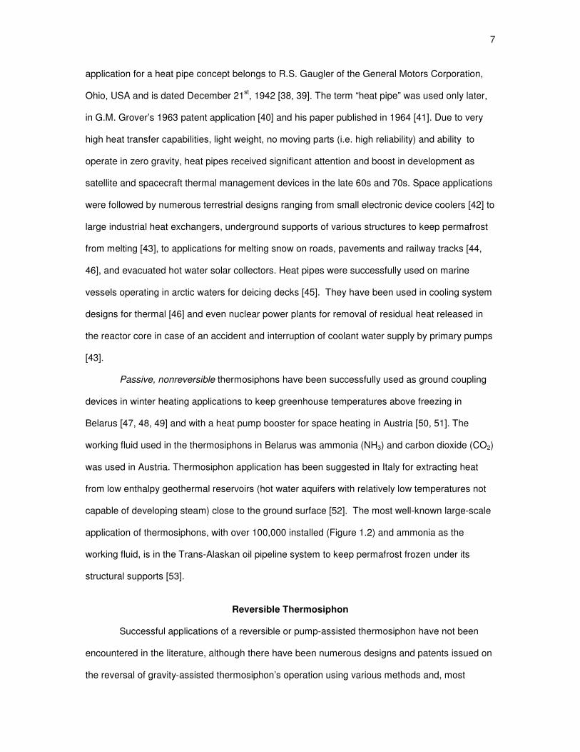
The most efficient thermal energy storage will be achieved when an array of
thermosiphons (Figure 1.5) is used to transfer heat to/from the ground. This configuration would
minimize heat or “cold” dissipation to the periphery and allow internal thermosiphons to efficiently
use precooled or preheated soil by neighboring thermosiphons.
Qin
Qin Qin
Thermosiphon
Evaporation
Soil Soil
Liquid
Vapor
Qout
Qout
Qout
Convection

10
Figure 1.4: Reversible thermosiphon operation – heat injection.
For increasing the effectiveness of summer cooling (air conditioning), the temperature of
soil can be lowered by employing a working fluid with a low boiling temperature in the
thermosiphon (i.e. refrigerant R134a or other more benign new alternatives like DuPont™
Opteon™ XP10 which is based on HFO-1234yf and has lower Global Warming Potential (GWP),
being released on the market by DuPont [57]). Lowering the soil temperature below 0°C would
cause cyclic freezing and melting of surrounding water in the ground which would drastically
increase the storage capacity of the moist porous medium.
Air Conditioning or Space Cooling Potential
Based on the above-described concepts, an air conditioning system, which requires very
little auxiliary energy input and, subsequently, has a very high COP, can be developed.
Qout
Qout Qout
Soil Soil
Reversible
Thermosiphon
Vapor
Liquid
Qin
Qin Qin
Small Pump
Condensation
Convection
11
Figure 1.5: Array of thermosiphons.
Widespread use of these low-power air conditioning systems would make a significant impact on
the ever-increasing demand of energy, most of which is currently supplied by fossil fuels. For this
new technology to be implemented on a mass scale, and to compete with other technologies, its
installation and operational costs, as well as its performance and reliability, should be comparable
to those of existing air conditioning or GSHP installations. Low operational costs and high
reliability should be easily achievable due to the inherent simplicity of the heat pipes and few
moving parts needed for such a system. New, cheaper drilling methods are also becoming
available (the biggest anticipated cost in this type of system), like a push-down method of
inserting heat exchanger pipes in the ground. In locations with softer, clay type soils, the method
has already been successfully tested [58]. This new technology seems promising and experience
and knowledge gained in preparation of the present study should supply additional insight for its
future development.
The biggest obstacle to making these systems feasible is the yet unknown system
performance characteristics and its sizing methods, which directly affect the required material and
installation costs. The design parameters, like anticipated heat transfer rates per unit length (or
Internal thermosiphon
Peripheral thermosiphon

12
per unit surface area) of the thermosiphon pipe, in addition to temperature difference (driving
potential) between the ambient air (or the air being cooled) and the soil, would primarily depend
on heat transfer in the ground. Characterization of the heat transfer mechanism and experimental
assessment of the expected heat transfer rates are the main purpose of this study. Particularly
interesting is the potential enhancement to heat transfer in the soil due to natural convection and
the conditions of its occurrence.

13
References
[1] U.S. Energy Information Administration (EIA), 2009, “Energy Consumption by Sector,” Annual Energy Review 2008, Report No. DOE/EIA-0384(2008). http://www.eia.doe.gov/emeu/aer/pdf/pages/sec2.pdf (Accessed on March 26, 2010).
[2] Neal, W. E. J., 1981,”Thermal Energy Storage,” The Institute of Physics, Journal of Phys.
Technology, 12, pp. 213-226. [3] Nielsen, K., 2003, “Thermal Energy Storage – A State-of-the-Art,” A report within the
research program Smart Energy-Efficient Buildings at Norwegian University of Science and Technology (NTNU) and SINTEF 2002-2006. Trondheim, January 2003.
[4] Faninger, G., 2005. “Thermal Energy Storage,” International Energy Agency’s Solar
Heating and Cooling Programme, Task 28-2-6, http://www.nachhaltigwirtschaften.at/pdf/task28_2_6_Thermal_Energy_Storage.pdf (Accessed on March 26, 2010).
[5] Solar Ponds: http://www.solarponds.com (Accessed on Apr 21, 2011). [6] Solar Ponds: http://www.globalwarmingnet.info/solar-energy/solar-ponds.html (Accessed
on Apr 21, 2011). [7] Solar Ponds: http://www.solarthermalmagazine.com/learn-more/solar-ponds/ (Accessed
on Apr 21, 2011). [8] Solar Pond: http://en.wikipedia.org/wiki/Solar_pond (Accessed on Apr 21, 2011).
[9] Ice storage air conditioning: http://en.wikipedia.org/wiki/Ice_storage_air_conditioning (Accessed on Apr 24, 2011).
[10] Gabrielsson, A., Bergdahl, U., Moritz, L., 2000, “Thermal Energy Storage in Soils at
Temperatures Reaching 90°C,” Transactions of the ASME, Journal of Solar Energy Engineering, 122(2), pp. 3-8.
[11] Hauer, A., 2006, “Innovative Thermal Energy Storage Systems for Residential Use,”
Proceedings of the 4th International Conference on Energy Efficiency in Domestic Appliances and Lighting – EEDAL’06, London, UK.
[12] Reuss, M., Mueller, J. P., Roehle, B., Weckler, M., Schoelkopf , W., 1998, “A New
Concept of a Hybrid Storage System for Seasonal Thermal Energy Storage in Solar District Heating,” The Second Stockton International Geothermal Conference Proceedings. March 16 and 17, 1998.
[13] Ball, D. A., Fischer, R. D., Talbert, S. G., 1983, “State-of-the-Art Survey of Existing
Knowledge for the Design of Ground-Source Heat Pumps,” Battelle, Columbus, Ohio. [14] Ball, D. A., Fischer, R. D., Hodgett, D. L., 1983, “Design Methods for Ground-Source
Heat Pumps,” ASHRAE Trans., 89(2B), pp. 416-440. [15] Svec, O. J., 1987, "Potential of Ground Heat Source Systems," International Journal of
Energy Research, 11, pp. 573–581. doi: 10.1002/er.4440110413. [16] ME Staff, 1983, “Seasonal Thermal Energy Storage,” Journal of Mechanical Engineering,
3, pp. 28-34.

14
[17] Nordell, B., Hellstrom, G., 2000, “High Temperature Solar Heated Seasonal Storage System for Low Temperature Heating of Buildings,” Solar Energy, 69(6), pp. 511-523.
[18] van Meurs, G. A. M., 1985, “Seasonal Heat Storage in the Soil,” Doctoral dissertation,
Dutch Efficiency Bureau – Pijnacker. [19] Schmidt, T., Mangold, D., 2006, “New Steps in Seasonal Energy Storage in Germany,”
Ecostock 2006 Proceedings, Tenth International Conference on Thermal Energy Storage, May 31-June 2, 2006, Pomona, USA.
[20] Mangold, D., Schmidt, T., 2007, “The Next Generations of Seasonal Thermal Energy
Storage in Germany,” ESTEC 2007, München. [21] Schmidt, T., Mangold, D., 2008, “Solare Nahwärme mit Langzeit-Wärmespeicherung in
Deutschland,” Zeitschrift: erneuerbare energie, 4, http://www.aee.at/publikationen/zeitung/2008-04/08.php (Accessed on Apr 21, 2011).
[22] Drake Landing Solar Community, Okotoks, Alberta, Canada, http://www.dlsc.ca
(Accessed on Apr 21, 2011). [23] Midttømme, K., Banks, D., Ramstad, R. K., Sæther, O. M., Skarphagen, H., 2008,
“Ground-Source Heat Pumps and Underground Thermal Energy Storage - Energy for the Future,” in Slagstad, T. (ed.) Geology for Society, Geological Survey of Norway, Special Publication, 11, pp. 93–98, http://www.ngu.no/upload/Publikasjoner/Special%20publication/SP11_08_Midttomme_HI.pdf (Accessed on Apr 21, 2011).
[24] Wong, B., Snijders, A., McClung, L., 2006, "Recent Inter-seasonal Underground Thermal
Energy Storage Applications in Canada," EIC Climate Change Technology, 2006 IEEE , pp. 1-7, 10-12 May, 2006, SAIC Canada, Ottawa, ON, doi: 10.1109/EICCCC.2006.277232, http://ieeexplore.ieee.org/stamp/stamp.jsp?tp=&arnumber=4057362&isnumber=4057291 (Accessed on Apr 21, 2011).
[25] Yanshun Y., Zuiliang M., Xianting L., 2008, "A New Integrated System with Cooling
Storage in Soil and Ground-coupled Heat Pump," Applied Thermal Engineering, 28(11-12), August 2008, pp. 1450-1462, ISSN 1359-4311, doi: 10.1016/j.applthermaleng.2007.09.006.
[26] Spitler, J. D., 2005, “Ground Source Heat Pumps System Research – Past, Present and
Future" (Editorial), International Journal of HVAC&R Research. 11(2), pp. 165-167. [27] Lund, J., et al., 2004, “Geothermal (Ground-Source) Heat Pumps – A World Overview,”
Geo-Heat Center Bulletin, September 2004. [28] Straube, J., 2009, “Ground Source Heat Pumps (Geothermal) for Residential Heating and
Cooling: Carbon Emissions and Efficiency,” Building Science Digest 113. http://www.buildingscience.com/documents/digests/bsd-113-ground-source-heat-pumps-geothermal-for-residential-heating-and-cooling-carbon-emissions-and-efficiency?full_view=1 (Accessed on April 15, 2010).
[29] Svec, O. J., Goodrich, L. E., Palmer, J. H. L., 1983, “Heat Transfer Characteristics of In-
ground Heat Exchangers,” Journal of Energy Research, 7, pp. 265-278. [30] Bernier, M. A., 2006, “Closed-Loop Ground-Coupled Heat Pump Systems,” ASHRAE
Journal, September 2006.
15
[31] Hamada, Y., Nakamura, M., Saitoh, H., Kubota, H, Ochifuji, K., 2007, “Improved
Underground Heat Exchanger by Using No-Dig Method for Space Heating and Cooling,” Renewable Energy, 32, pp. 480-495.
[32] Angelotti, A., Pagliano, L., Solaini, G., 2004, ”Summer Cooling by Earth-to-Water Heat
Exchangers: Experimental Results and Optimisation by Dynamic Simulation,” Proc. EuroSun2004, Freiburg, Germany, pp. 2-678.
[33] Direct-Exchange Geothermal Heating/Cooling Technology:
http://www.copper.org/applications/plumbing/heatpump/geothermal/gthrml_main.html (Accessed on Apr 24, 2011).
[34] Direct Exchange (DX) Geothermal Heat Pumps:
http://digtheheat.com/geothermal_heatpumps/DX_geothermal.html (Accessed on Apr 24, 2011).
[35] Direct Exchange Geothermal Heat Pump:
http://en.wikipedia.org/wiki/Direct_exchange_geothermal_heat_pump (Accessed on Apr 24, 2011).
[36] Udell, K. S., Jankovich, P., Kekelia, B., 2009, “Seasonal Underground Thermal Energy
Storage Using Smart Thermosiphon Technology,” Transactions of the Geothermal Resources Council, 2009 Annual Meeting, Reno, NV, 33, pp. 643-647.
[37] Udell, K. S., Kekelia, B., Jankovich, P., 2011, “Net Zero Energy Air Conditioning Using
Smart Thermosiphon Arrays,” 2011 ASHRAE Winter Conference, ASHRAE Transactions, 117(1), Las Vegas, NV.
[38] Dunn, P. D., Reay, D. A., 1994, “Heat Pipes,” 4
th ed., Pergamon, Oxford, England.
[39] Gaugler, R. S., 1944, “Heat Transfer Device,” US Patent, No. 2350348, Appl. Dec 21,
1942. Published June 6, 1944. [40] Grover, G. M., 1966, “Evaporation-Condensation Heat Transfer Device,” US Patent, No.
3229759, Appl. Dec 2, 1963. Published Jan 18, 1966. [41] Grover, G. M., Cotter, T. P., Erickson, G. F., 1964, “Structures of Very High Thermal
Conductance,” J. Appl. Phys., 35, p. 1990. [42] Osakabe, T., et al, 1981, “Application of Heat Pipe to Audio Amplifier,” in Advances in
Heat Pipe Technology: Proceedings of the IVth International Heat Pipe Conference, Edited by Reay, D. A., Pergamon, Oxford, pp. 25-36.
[43] Commission of the European Communities, 1987, “Heat Pipes: Construction and
Application. A study of Patents and Patent Applications,” Edited by Marten Terpstra and Johan G. van Veen, Elsevier Applied Science, London and New York.
[44] Tanaka, O., et al., 1981, “Snow Melting Using Heat Pipe,” in Advances in Heat Pipe
Technology: Proceedings of the IVth International Heat Pipe Conference, Edited by Reay, D. A., Pergamon, Oxford, pp. 11-33.
[45] Matsuda, S., et al, 1981, “Test of a Horizontal Heat Pipe Deicing Panel for Use on Marine
Vessels,” in Advances in Heat Pipe Technology: Proceedings of the IVth International Heat Pipe Conference, Edited by Reay, D. A., Pergamon, Oxford, pp. 3-10.

16
[46] Robertson, A. S., Cady, E. C., 1981, “Heat Pipe Dry Cooling for Electrical Generating Stations,” in Advances in Heat Pipe Technology: Proceedings of the IVth International Heat Pipe Conference, Edited by Reay, D. A., Pergamon, Oxford, pp. 745-758.
[47] Vasiliev, L. L, et al., 1981, ”Heat Transfer Studies for Heat Pipe Cooling and Freezing of
Ground,” in Advances in Heat Pipe Technology: Proceedings of the IVth International Heat Pipe Conference, Edited by Reay, D. A., Pergamon, Oxford, pp. 63-72.
[48] Vasiliev, L. L, et al., 1984, ”Heat Pipes and Heat Pipe Exchangers for Heat Recovery
Systems,” Heat Recovery Systems, Pergamon Press, London, 4(4), pp. 227-233. [49] Vasiliev, L. L, 1987, ”Heat Pipes for Heating and Cooling the Ground,” Inzhenerno-
Fizicheskii Zhurnal (Russian), 52(4), pp. 676-687. [50] Rieberer, R., 2005, “Naturally Circulating Probes and Collectors for Ground-Coupled
Heat Pumps," International Journal of Refrigeration, 28, pp. 1308-1315. [51] Ochsner, K., 2008, “Carbon Dioxide Heat Pipe in Conjunction with a Ground Source Heat
Pump (GSHP),” Applied Thermal Engineering, 28, pp. 2077-2082. [52] Cannaviello, M., et al, 1981, “Gravity Heat Pipes as Geothermal Convectors,” in
Advances in Heat Pipe Technology: Proceedings of the IVth International Heat Pipe Conference, Edited by Reay, D. A., Pergamon, Oxford, pp. 759-766.
[53] Heuer, C. E., 1979, “The Application of Heat Pipes on the Trans-AlaskaPipeline,” Special
Report 79-26, US Army Corps of Engineers, Cold Regions Research and Engineering Laboratory, Hanover, NH.
[54] Basiulis, A., 1977, “Heat Pipe Capable of Operating Against Gravity and Structures
Utilizing Same,” Hughes Aircraft Company, US Patent, No. 4057963, Appl. March 11, 1976. Published November 15, 1977.
[55] Kosson, R., 1981, “Down Pumping Heat Transfer Device,” Grumman Aerospace
Corporation, US Patent, No. 4252185, Appl. Aug 27, 1979. Published Feb 24, 1981. [56] Roberts, C. C. Jr., 1981, “A Review of Heat Pipe Liquid Delivery Concepts,” in Advances
in Heat Pipe Technology: Proceedings of the IVth International Heat Pipe Conference, Edited by Reay, D. A., Pergamon, Oxford, pp. 693-702.
[57] News release by DuPont on Oct 14, 2010 in Nuremberg, Germany:
http://www2.dupont.com/Refrigerants/en_US/news_events/article20101014.html (Accessed on Apr 11, 2011).
[58] Hollenhorst, J., 2011, "University Scientists Begin Tests on 'Ice Ball' Air Conditioning,"
News story on: http://www.ksl.com/?nid=148&sid=13892019 (Accessed on Apr 24, 2011).

2. PROBLEM FORMULATION AND METHODS
In this chapter, a theoretical model for the heat transfer from/to the thermosiphon to/from
the storage medium (soil) will be defined and methods for the estimation of the heat transfer rates
will be identified. As noted in the previous chapter, if an array of thermosiphons is used to create
a UTES bank (Figure 1.5), a large number of heat exchange cells with similar boundary
conditions will be formed. Thus, the study of one such cell would apply to much of a multicell
domain.
Heat Transfer Domain
If we consider an internal thermosiphon and draw lines of symmetry between neighboring
thermosiphons, the boundaries will form a hexagon. These lines of symmetry represent adiabatic
boundaries, as conditions from both sides of the boundaries are the same (temperature gradient
at the boundary is zero, EFEG = 0, where ! is the direction normal to the cell boundary), and, thus,
there is no heat transfer across those boundaries. For modeling thermal energy storage behavior
in the array, a single cell with a thermosiphon in the center (as shown in Figure 2.1) can be
considered. To simplify the problem, the hexagonal boundary can be approximated with a circular
one (Figure 2.1), so that the volume of the porous medium encompassed (i.e. energy stored)
within both boundaries are equal.
Cross-section and anticipated heat transfer processes in such a cylinder are shown in
Figure 2.2. In order to increase the energy storage capacity, freezing of ground water is desirable,
but to avoid a negative effect on near-surface underground flora and fauna due to freezing the
soil, and minimize the heat losses from the ground surface, the top portion of the thermosiphons
should be insulated (see Figure 2.2).

18
Figure 2.1: Top view of an internal thermosiphon cell in an array of thermosiphons. Also shown is
an equivalent circular boundary that would approximate an actual hexagon.
For certain temperatures and ground porosities/permeabilities, natural convection may
also arise which would enhance the heat transfer to/from UTES. For the reason of studying the
fundamental conditions where natural convection enhancement occurs, porous media
permeabilities were chosen to increase the probability of seeing the natural convection during
experiments. Without convection, the freezing/thawing of the medium is often referred to as a
Stefan problem1 and is discussed in the following section.
Theoretical Model
Heat transfer problems with moving boundaries of the melting/solidification front are
known as Stefan problems. The phase change front position is unknown and has to be
determined as part of the solution. Heat flux across the phase boundary is not continuous and the
heat equation is replaced by a flux condition which relates the velocity of the moving phase
boundary with the jump of the heat flux. The problem is nonlinear and can be solved analytically
for only a limited number of cases [1]. For the time-varying boundary conditions of temperature or
heat flux, it has to be solved numerically.
There are two main approaches to solving Stefan problems: One is the front-tracking
method, in which the phase boundary is tracked and either the isotherms (the phase boundary
1 From Wikipedia: "The problem is named after Jožef Stefan, the Slovene physicist who introduced the general class of
such problems around 1890, in relation to problems of ice formation. This question had been considered earlier, in 1831, by Lamé and Clapeyron."
Thermosiphon
Replacing hexagon with
circular boundary

19
Figure 2.2: Heat injection in the soil for a cylindrical cell (vertical cross-section).
being one of them) are followed, or a variable space grid and variable time step are employed to
place the phase change front on nodes which change location in space [2].
The second approach uses a fixed space domain and using temperature, or more
commonly, a temperature-dependent enthalpy function as an independent variable and a so-
called “mushy” zone (a partially solidified region with liquid fraction between 0 and 1) to solve the
problem [3,4,5,6].
For the purposes of this study, in order to illustrate the significance of Rayleigh number
as a driving parameter in heat transfer from/to the thermosiphon to/from the soil, the stream
function formulation of the problem will be presented. The following assumptions are made: (a)
the porous medium is homogeneous and isotropic, (b) physical properties: density and viscosity,
as well as (c) thermal properties: heat capacity, conductivity and coefficient of thermal expansion,
are constant (variations in density are significant only in the buoyancy driving force), (d) the flow
is sufficiently slow (Re < 1) to allow application of Darcy's law, and fluid and porous matrix are in
local thermal equilibrium (i.e. H = I = J = ), (e) the flow is two dimensional, (f) the volume
change due to freezing is negligible.
The following volume fractions of the porous media are defined:
Ice
Water saturated soil
Thermosiphon
Insulation
Q
Q
Q
Convection Convection
Adiabatic
boundary
Ground surface
20
Porosity of the medium:
= 0KLM+0 (2.1)
Fraction of liquid in void volume:
4 = 0H0N (2.2)
Fraction of liquid in volume element:
5 = 0H0 = 4 (2.3)
Applying the previously mentioned simplifying assumptions, the governing equations for
the porous media can be defined as follows:
Continuity: ∇ ∙ . = 0 (2.4)
Momentum: . 7 = −∇p − ρg (2.5)
Energy: 6TJ∇UT − .9NT,N∇T = 9WWW XX- (2.6)
where volume averaged thermal conductivity of porous media, 6TJ, can be calculated using one
of the porous medium conductivity models reviewed in Chapter 3 and the mean thermal
capacitance (volumetric heat capacity) of the mixture is given by:
9WWW = 9NT,N + (1 − )9JJ (2.7)
Using the stream function definition for cylindrical, axi-symmetric domain:

21
.\ = −1' X<X1 !.] = 1' X<X' (2.8)
where .\ is the velocity in the ' direction and .] is the velocity in the 1 direction. Note that,
since:
XU<X1X' = XU<X'X1 (2.9)
the stream function definition (Equation (2.8)) satisfies the continuity equation for 2D axi-
symmetric domain (Equation (2.10)) for negligible density variations (9 ≈ ! -): 1r ∂(r.\)∂r + ∂(.])∂z = 0
(2.10)
For flow in homogeneous isotropic porous media, the velocities in the radial and vertical
directions are:
.\ = −μ X"X' !.] = −μ X(" + 91)X1 (2.11)
If the gravitational acceleration is opposite to the direction of 1, solving for the pressure
gradients in Equation (2.11) and cross-differentiating, the following equations are derived:
XU"X'X1 = −μ X.\X1 (2.12a)
XU"X1X' = −μ X.]X' − X9X' (2.12b)
By subtracting the (2.12b) from (2.12a), dividing by the fluid viscosity, μ, multiplying by
the media permeability, , and rearranging, the following relationship is derived:
22
X.\X1 − X.]X' = μ X9X' (2.13)
Assuming that slight variations in density are proportional to temperature variations
(Boussinesq approximation) the fluid density can be specified as:
9 = 9c − 9c3( − c) (2.14)
where β is the thermal expansion coefficient and is defined as:
3 = − 19c dX9XeT (2.15)
Equation (2.13) can be written as:
X.\X1 − X.]X' = μ X9X XX' (2.16)
Solving the Equation (2.15) for EfEF and substituting it in Equation (2.16) yields:
X.\X1 − X.]X' = −39cμ XX' (2.17)
The relationship between the stream function, <, and the temperature field in the porous
medium is defined by differentiating the velocities specified in Equation (2.8) and then substituting
into Equation (2.16):
XU<X'U − 1' X<X' + XU<X1U = 38 ' XX' (2.18)
where ν is the fluid kinematic viscosity:
23
8 = μ9c (2.19)
The temperature field is obtained from the solution of the energy equation (Equation
(2.6)), which, after substitution of the fluid velocities from Equation (2.8), for 2D axi-symmetric
domain is written as:
1' XX' g' XX'h + XUX1U + 1' X<X1 9NT,N6TJ XX' − 1' X<X' 9NT,N6TJ XX1 = 12TJ XX- (2.20)
where the thermal diffusivity for porous medium, 2TJ, can be calculated from:
2TJ = 6TJ9WWW (2.21)
Defining a following ratio:
= = 9NT,N9NT,N + (1 − )9JJ (2.22)
and introducing nondimensional variables:
<i = <2TJ
' = '
1 = 1
W = ( − k)(I − k) = 2TJ-U
(2.23)

24
including a Rayleigh number, (, which characterizes the strength of free convection. For porous
media, the Rayleigh number is defined as:
( = 3(I − k)2TJ8 (2.24)
Using the scaling defined in Equations (2.22) to (2.24), the following dimensionless forms
of Equations (2.18) and (2.20) can be written:
XU<iX'U − 1' X<iX' + XU<iX1U = (' XWX' (2.25)
XUWX'U + 1' XWX' + XUWX1U + =' X<iX1 XWX' − =' X<iX' XWX1 = XWX (2.26)
From Equations (2.25) and (2.26) it can be seen that as Ra increases, the stream
function and its derivatives increase (see Equation (2.25)). Thus, the advection terms in the
energy equation (Equation (2.26)) become significant. For very small Ra (very weak natural
convection), the advection terms become negligible and conduction becomes the main
contributor to the heat transfer. Equation (2.25) also shows that as the radial temperature
gradient decreases (as temperature field becomes more uniform), the forcing function for
convection also disappears.
Maximum Fluid Velocity During Natural Convection in Porous Medium
If we consider a heat extraction from the porous medium with initial temperature k, as
the temperature on the outside wall of the thermosiphon decreases to I, a positive radial
temperature gradient, EFE\ , develops. As defined by Equation (2.17), that gradient will induce fluid
flow, which allows for convective heat flow, potentially enhancing the heat transfer to the
thermosiphon.

25
Of interest is the strength of the convective flow, characterized by the maximum fluid
velocity. From results of other studies [5, 7], and the numerical simulations presented in Chapter
6 of this dissertation, the maximum fluid velocity is found next to the thermosiphon pipe wall near
the midpoint of the domain’s depth. At that location, the velocity in the radial direction, .\, is
essentially zero and remains zero above and below the midpoint for nearly half of the total
thermosiphon length. Thus, ElmE] = 0, and Equation (2.17) becomes:
X.]X' = ((I − k) 2TJ XX' (2.27)
Integration of Equation (2.27) with respect to ' produces:
.] = ((I − k) 2TJ n XX'\\∗ '
(2.28)
where '∗ is the radial location of a point of zero vertical velocity (.] = 0), a location where,
presumably, the temperature is still at the temperature of the far-field ( k). Thus:
.] = ( 2TJ ( − k)(I − k) (2.29)
and:
.]Jpq = ( 2TJ (2.30)
Equation (2.30) can be used to estimate the maximum fluid velocity and, thus, the
strength of the anticipated natural convection in the porous medium.

26
Methods for Estimating Heat Transfer Rates to/from Porous Medium
In order to assess the heat injection/extraction rates to/from the porous medium in the
cylindrical cell, three methods were employed: (1) the time rate of change of the total thermal
energy content of the porous medium, calculated from the readings of thermocouples placed in
the porous medium bed, yielding the heat injected/extracted for the given time step; (2) heat
transfer rate to/from the air flowing through the heat exchanger calculated from the measured air
flow and the difference in air temperatures between the inlet and outlet of the heat exchanger;
and (3) thermosiphon’s overall heat transfer coefficient, /rs, estimated from the previous two
methods and the heat transfer rates calculated using the driving temperature difference between
the temperature of the porous medium on the outside wall of the thermosiphon and the inlet
temperature of the ambient air. While each of these methods suffers from relatively high error,
taken together, reasonable values of heat transfer rates were identified.
The first method. As the temperature distribution in the porous medium is not uniform
and changes with time, the volume of the cylindrical cell can be divided into a large number of
small (elemental) concentric rings (Figure 2.3) within which the temperature can be assumed to
be uniform. As the heat is injected or extracted from the ring, its temperature (or the phase of the
fluid filling its voids) changes. The energy injected/extracted into/from each ring during a specified
time can be calculated knowing the change in the temperature of the ring. Based on the changes
in temperature of the ring, the changes in the energy content of the rings were calculated and
summed for all rings for each time step.
The change in thermal energy content, t-, of the cylindrical cell of the porous medium
for any given time interval, -, can be calculated using the following equation (Equation (2.31)):
tr =u0Mvw9NN + (1 − )9JJxM + 9NℎNy (2.31)
where:
0M is volume of each elemental ring around a thermosiphon,
M is change in temperature of the ?-th ring during - time interval.
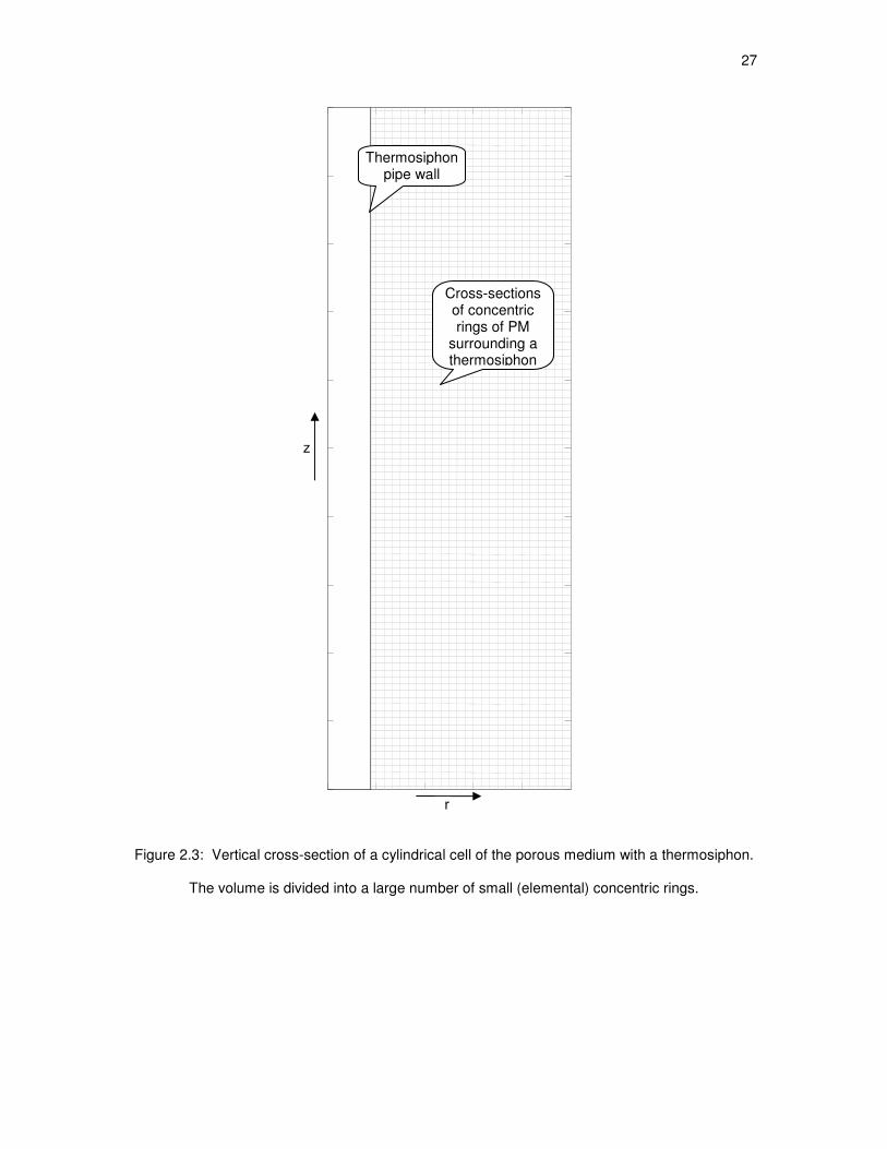
27
Figure 2.3: Vertical cross-section of a cylindrical cell of the porous medium with a thermosiphon.
The volume is divided into a large number of small (elemental) concentric rings.
r
z
Cross-sections of concentric rings of PM
surrounding a thermosiphon
Thermosiphon pipe wall

28
Dividing the change in energy content, t-, by the time, -, during which that change
occurred would yield the rate at which thermal energy was injected or extracted for the given
volume of the porous medium (Equation (2.32)).
%&TJ = tr- (2.32)
The second method. If the air flow rate, %, and the change in the temperature of the
bulk air, pM\, as it passes through the heat exchanger, used for the heat exchange with the
ambient air, is known (or can be measured), then the heat extracted/injected from/to the porous
medium can be determined using Equation (2.33):
%&pM\ = %9pM\T,pM\pM\ (2.33)
The change in the air temperature, pM\, can be determined measuring the bulk air
temperatures before and after passing through the heat exchanger. The volumetric flow rate of
air, %, can be measured with an orifice meter (see orifice meter schematics in Figure 2.4)
installed in the air supply duct (see Chapter 4 for the details of the experimental apparatus) and
measuring the static pressure difference across the orifice plate.
For the air flow rate calculations, the following equation (Equation (2.34)) is used [8]:
% = LLz 2(B − BU)9pM\(1 − 3L|) (2.34)
where:
(B − BU) is a static pressure difference between points 1 and 2, which can be
estimated measuring height difference, ∆h, of fluid columns in the U-tube
manometer (see Figure 2.4),

29
Figure 2.4: Orifice meter schematics for air flow measurements
3L = ~ is a ratio of the orifice diameter,L, to the diameter of the pipe/duct, ,
L is a cross-sectional area of the orifice,
L is an Overall Orifice Loss Coefficient.
The Overall Orifice Loss Coefficient, L, can be calculated with the Stolz [8] equation
(Equation (2.35)):
L = 0.5959 + 0.03123LU. − 0.18403L + 0.00293LU. 10()3Lc.
+ 0.0390 3L|1 − 3L| − 0.0158393L
(2.35)
where:
() = 49pM\7pM\ LLz 2(B − BU)9pM\(1 − 3L|) (2.36)
1/2D 1D Orifice plate
D 1 2
∆h

30
This method requires iterations as an initial guess for the Overall Orifice Loss Coefficient, L, is needed, then the Reynolds number, (), is calculated with the Equation (2.36), and
substituted into the Stolz equation (Equation (2.35)). The calculations are repeated until
convergence, with the desired tolerance, between the guessed and the calculated values of the L coefficient, is reached. The calculated L is used in Equation (2.34) to determine the
volumetric air flow rate % across the heat exchanger, which is then used to find the heat transfer
rate to/from the ambient air %&pM\ with the Equation (2.33).
The third method. Heat extraction/injection rate with a thermosiphon, %&rs, from/into the
porous medium can be related to the temperature difference between the average outer surface
of the thermosiphon pipe, pHH, and the ambient air, pM\, using an overall thermosiphon heat
transfer coefficient /rs, (see Equation (2.37)):
%&rs = /rs(pM\ − pHH) (2.37)
The overall thermosiphon heat transfer coefficient, /rs, can be estimated based on the
heat transfer rates calculated in the previous two methods. The validity of the estimated value can
also be checked as follows: As the temperatures inside the porous medium are being measured
during the experiment, it can be easily determined when all the water in the porous medium
freezes or thaws (assuming the phase change of water occurs at exactly 0°C). Knowing the
average initial temperature of the bulk material inside the tank, MGMr, its composition/porosity, ,
and thus, respective volumes of sand and water/ice, the total energy needed to cool and then
freeze (or warm up and then thaw) the porous medium can be calculated (see Equation (2.38)):
tN\]/rsp = 0TJvw9NN + (1 − )9JJx · (0° − MGMr) + 9NℎNy (2.38)
where:
>-subscript indicates fluid – water or ice (depending on the initial state of the fluid),

31
-subscript indicates solid matrix – sand/quartz.
The cumulative energy extracted/injected by the thermosiphon during the experiment, trs,lJlH, by the observed freezing/thawing time point, -TspIspG, calculated using the
estimated /rs in the Equation (2.39), should equal the total energy needed to cool and then
freeze (or warm up and then thaw) the porous medium, tN\]/rsp.
trs,lJlH = n %&rs-rrc = n /rs(pM\ − pHH)-r
rc (2.39)
All three of the above-described methods were used for the estimation of heat transfer
rates from/into the porous medium during the experiments and the results are presented in
Chapter 5.
Selection of Porous Media for the Experiments
It was expected that soils with relatively high permeability would facilitate development of
natural convection cells near the thermosiphon, thus enhancing heat transfer mechanism to/from
the thermosiphon wall. In order to assess this enhancement, the media had to be selected which
would yield natural convection (Ra numbers in the range of 10-40 or above [5, 9, 10]) for the
expected conditions of injecting or extracting heat in the soil. Sand (unconsolidated particles of
quartz) was chosen for the medium as it is a major constituent in a large variety of soil types and
its properties are well established. Different permeabilities of the sand pack can be obtained by
selecting different grain sizes of sand. As permeability affects Ra number (see Equation (2.24))
and, consequently, the natural convection in porous media, the Carman-Kozeny [11, 12] equation
(Equation (2.40)) was used to determine the needed average grain size of the sand for the
experiments. The Carman-Kozeny equation relates mean particle diameter, J, and porosity, ,
of the porous medium to its permeability, :

32
= JU180(1 − )U (2.40)
For the calculations of average grain size of sand, the following assumptions were made:
based on average porosities of naturally occurring sands [13, 14], porosity was taken as =40%; approximate temperature difference between the thermosiphon wall surface and the far-
field = (I − k) = 10 was used. The thermosiphon pipe length = 1 was
assumed and porous media properties (discussed in detail in Chapter 3) were based on near-
freezing (0°-10°C) temperatures of water. Figure 2.5 shows Ra number variation due to different
average grain sizes of sand for the above-listed conditions of porous media.
It can be seen from Figure 2.5 that Rayleigh numbers for the water-saturated sand with
0.5 mm mean diameter particles do not even reach 5 for the given conditions. For the sand pack
with 1.0 mm average grain size, Ra reaches approximately 10, which is the lower threshold for
seeing any natural convection effects in the porous medium [10]. For the 3.0 mm average grain
size sand pack, the permeability is high enough to allow Ra numbers to reach up to 80 for the
assumed conditions, presumably providing a strong natural convection potential.
It was decided to use two sizes of sand, one with fine (≈ 1 mm) grain size and another
with coarse (≈ 3 mm) grain size of particles. This range of grain sizes should capture the range of
soil permeabilities where natural convection enhancement would be expected. Further increasing
permeability beyond 3.0 mm mean diameter particles would have increased the natural
convection effects, but would have significantly deviated from common permeabilities of soil.
To segregate various grain sizes, construction sand was sieved using different mesh
numbers to yield a batch of fine sand containing particles in the range of 0.50 - 1.19 mm, and a
second batch of coarse sand containing particles in the size of 1.20 - 4.76 mm. While the
Carman-Kozeny equation (Equation (2.40)) provides a basis for choosing appropriate grain size
ranges for the experiments, it is not an accurate method of determining the actual bed
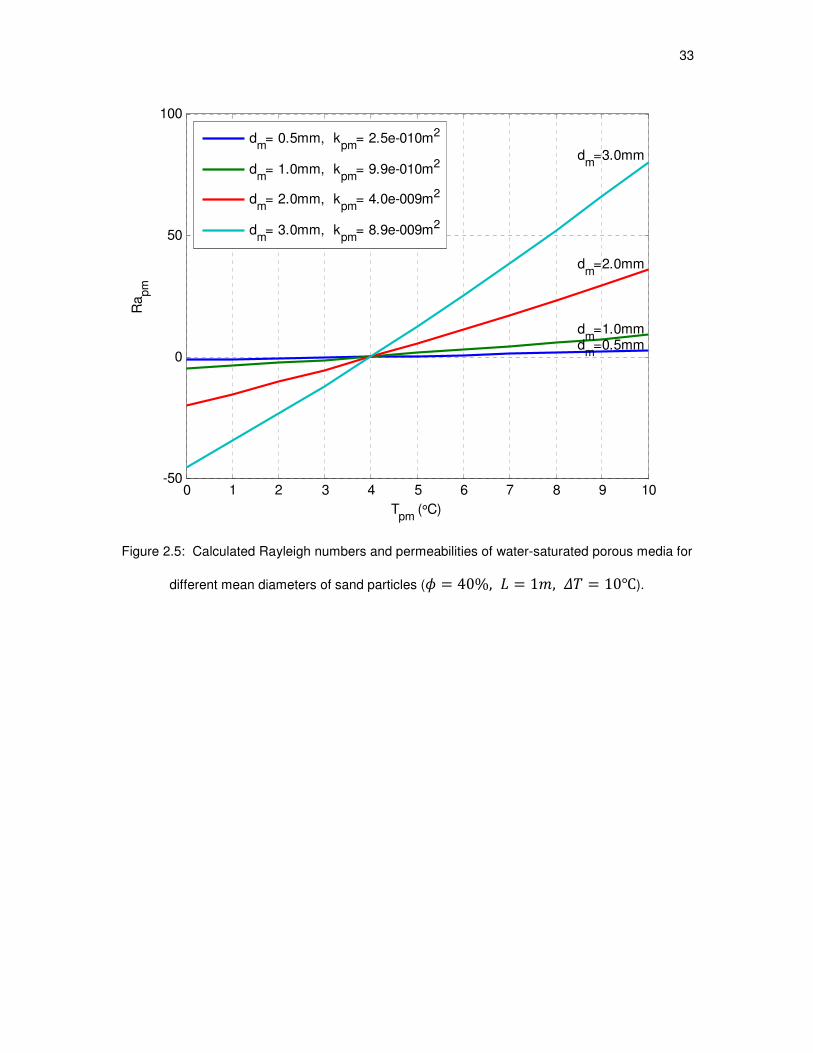
33
Figure 2.5: Calculated Rayleigh numbers and permeabilities of water-saturated porous media for
different mean diameters of sand particles ( = 40%, = 1, = 10).
0 1 2 3 4 5 6 7 8 9 10-50
0
50
100
Tpm
(°C)
Ra
pm
dm
=0.5mm d
m=1.0mm
dm
=2.0mm
dm
=3.0mm
dm
= 0.5mm, kpm
= 2.5e-010m2
dm
= 1.0mm, kpm
= 9.9e-010m2
dm
= 2.0mm, kpm
= 4.0e-009m2
dm
= 3.0mm, kpm
= 8.9e-009m2

34
permeability. Thus, the permeabilities of each batch of sand were measured experimentally (see
Chapter 3 for details).
35
References
[1] Carslaw, H. S., Jaeger, J. C., 1959, "Conduction of Heat in Solids," Clarendon Press, Oxford, 2nd Ed., pp. 282-296.
[2] Savovic, S., Caldwell, J., 2009, "Numerical Solution of Stefan Problem with Time-
Dependent Boundary Conditions by Variable Space Method," Thermal Science, 13(4), pp. 165-174.
[3] Savovic, S., Caldwell, J., 2003, "Finite Difference Solution of One-Dimensional Stefan
Problem with Periodic Boundary Conditions," Int. J. Heat and Mass Transfer, 46(15), pp. 2911-2916.
[4] Beckermann, C., Viskanta, R., 1988, "Natural Convection Solid/Liquid Phase Change in
Porous Media," Int. J. Heat and Mass Transfer, 31(1), pp. 35-46. [5] Chellaiah, S., Viskanta, R., 1989, "Freezing of Water-Saturated Porous Media in the
Presence of Natural Convection: Experiments and Analysis," J. of Heat Transfer, Transactions of the ASME, 111, pp. 425-432.
[6] Budak, B. M., Solovieva, E. N., Uspenskij, A. B., 1965, “Difference Method with
Smoothing Coefficients for Solving the Stefan Problems,” J. of Comput. Math. and Math. Physics in Russian, 5(5), pp. 828-840.
[7] Yucel, A., 1990, "Natural Convection Heat and Mass Transfer Along a Vertical Cylinder in
a Porous Medium,” Int. J. Heat and Mass Transfer, 33(10), pp. 2265-2274. [8] Janna, W. S., 1998, “Design of Fluid Thermal Systems,” 2
nd ed., PWS Publishing,
Boston, pp. 211-214. [9] Reda, D. C., 1986, “Natural Convection Experiments in a Stratified Liquid-Saturated
Porous Medium,” Transactions of the ASME, 108, pp. 660-666. [10] Oosthuizen, P. H., 1988, "The Effects of Free Convection on Steady State Freezing in a
Porous Medium-Filled Cavity," ASME Proc. 1988 National Heat Transfer Conference, HTD-96, 2, Houston, July 24-27, pp. 321-327.
[11] Carman, P. C., 1937, "Fluid Flow Through Granular Beds," Trans. lnst. Chem. Engrs., 15,
pp. 150-166. [12] Udell, K. S., 2006, Lecture notes for course MEEN 7960 “Multiphase Transport in Porous
Media”, University of Utah, Department of Mechanical Engineering, Salt Lake City, UT, USA.
[13] Total Porosity: http://web.ead.anl.gov/resrad/datacoll/porosity.htm (Accessed on July 10,
2011). [14] Geology: Porosity - Cliff’s Notes:
http://www.cliffsnotes.com/study_guide/Porosity.topicArticleId-9605,articleId-9528.html (Accessed on July 10, 2011).
3. PROPERTIES OF POROUS MEDIA
For accurate calculations and analysis of experimental results, properties of studied
porous media are defined in this chapter. First, porosity and permeability of the two different
average grain size sand packs were measured. Then, functions for temperature-dependent
properties of all three phases, sand, water and ice, were determined. For convenience of
calculations and ease of defining material properties in numerical modeling software ANSYS
Fluent (see Chapter 6) as temperature-dependent polynomial functions, the property data were
curve-fitted with 3rd
or 4th degree polynomials.
Porosity and Permeability
As exact porosity and the particle size distribution in the prepared sand packs was not
known, experiments were performed to determine their porosity and permeability. Porosity, , as
defined by the Equation (3.1), is a ratio of the volume of voids to the total volume occupied by the
porous medium.
= 0KLM+0rLrpH (3.1)
Porosity of the sand pack can be easily determined by packing it in a vessel with known
volume and adding a measured amount of fluid (water) up to its complete saturation. Porosities of
both sand packs were experimentally determined to be NMG = 0.38 ± 0.0753 and
Lp\I = 0.40 ± 0.0758 for the fine and coarse sand packs, respectively.
Finding permeability of the chosen porous media proved to be a little more challenging.
Hydraulic conductivity and permeability measurements of soil are often performed by
hydrologists, civil, geotechnical, and hydraulic engineers and others involved with groundwater

37
flow studies. Permeability, k, as defined in Darcy's law (Equations (3.2), (3.5), (3.6)) and
illustrated in Figure 3.1, characterizes the ability of a porous medium to conduct a fluid. It does
not depend on fluid properties and, thus, should not be confused with hydraulic conductivity, K,
which is the porous medium's ability to conduct water specifically.
% = − ℎ = − ℎ@ (3.2)
where:
Q is volumetric flow rate (m3/s),
A is bulk cross-sectional area in the direction of flow (m2),
L is length of flow passage in porous medium (m),
K is hydraulic conductivity (m/s),
ℎ is change in hydraulic head (m),
+s+H is hydraulic head gradient.
Using the definition of Darcy's velocity, q (Equation (3.3)), which is the volumetric flow
rate per unit bulk cross-sectional area in the direction of flow and has units of velocity (m/s),
Figure 3.1: Illustration of Darcy's Law.
Q
∆h
L
A
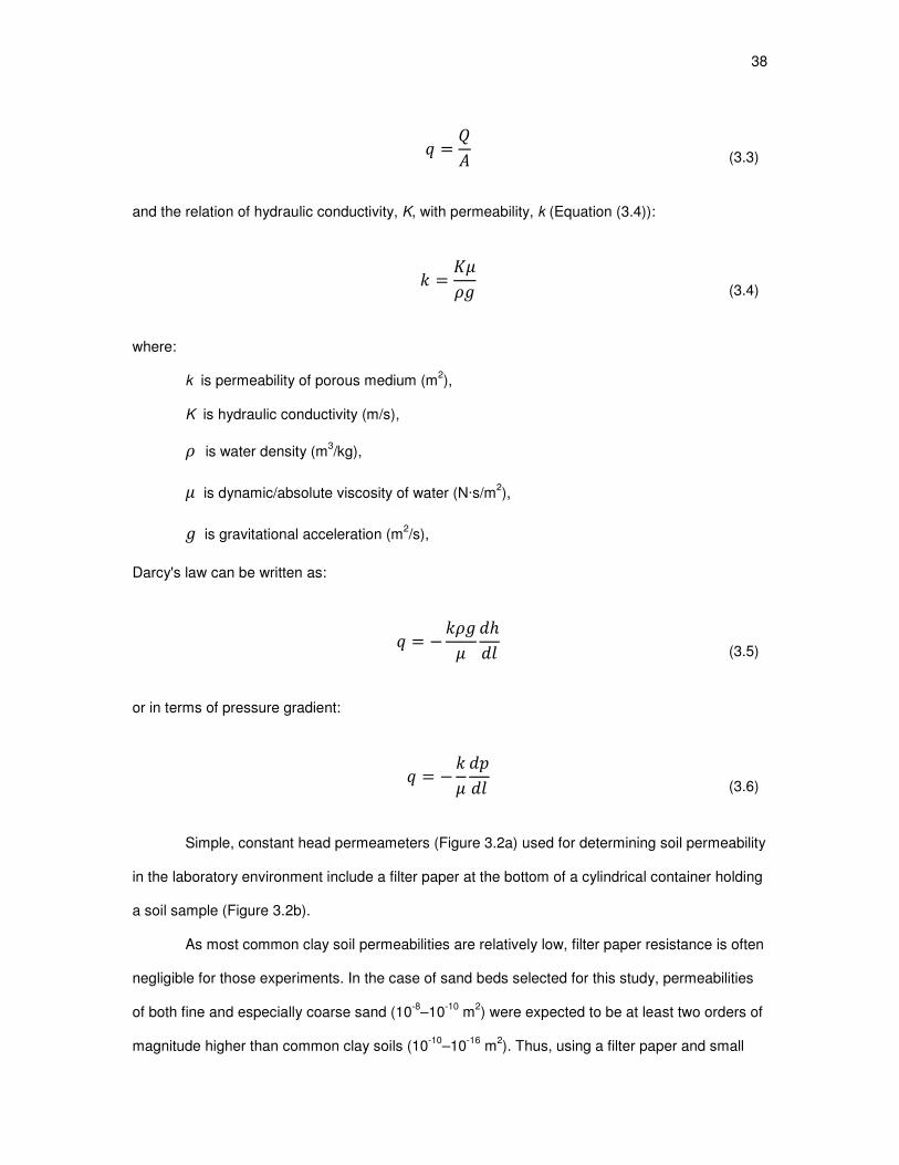
38
# = % (3.3)
and the relation of hydraulic conductivity, K, with permeability, k (Equation (3.4)):
= 79 (3.4)
where:
k is permeability of porous medium (m2),
K is hydraulic conductivity (m/s),
9 is water density (m3/kg),
7 is dynamic/absolute viscosity of water (N·s/m2),
is gravitational acceleration (m2/s),
Darcy's law can be written as:
# = −97 ℎ@ (3.5)
or in terms of pressure gradient:
# = −7 B@ (3.6)
Simple, constant head permeameters (Figure 3.2a) used for determining soil permeability
in the laboratory environment include a filter paper at the bottom of a cylindrical container holding
a soil sample (Figure 3.2b).
As most common clay soil permeabilities are relatively low, filter paper resistance is often
negligible for those experiments. In the case of sand beds selected for this study, permeabilities
of both fine and especially coarse sand (10-8
–10-10
m2) were expected to be at least two orders of
magnitude higher than common clay soils (10-10
–10-16
m2). Thus, using a filter paper and small

39
(a)
(b)
Figure 3.2: Constant head permeameter for determining soil permeability in the lab environment:
(a) simple permeameter with constant head, (b) filter paper and narrow inlet/outlet passage
valves adding resistance to water flow.
diameter inlet and outlet in the permeameter would have added a significant resistance to the
water flow. For more accurate measurements, it was decided to modify the experimental
apparatus. In order to measure a larger pressure drop within the porous medium, the length of
the cylinder, holding a sample, was doubled (Figure 3.3a). For reducing resistance to the flow
from the apparatus, its inlet and outlet diameters were significantly increased, valves were
eliminated, and instead of filter paper, aluminum screens were used (Figure 3.3b and Figure
3.3c).
Using the redesigned apparatus shown in Figure 3.3, permeabilities of both sand packs
were experimentally determined to be: kfine=1.93·10-10
m2 (195 Darcy) and kcoarse=2.03·10
-9 m
2
(2059 Darcy) for the fine and coarse sand packs, respectively.
Filter paper
Inlet valve
Outlet valve
Permeameter

40
(a)
(b)
Figure 3.3: Redesigned permeameter: (a) doubled cylinder length, (b) increased inlet/outlet
diameter and no valves are shown, (c) filter paper was replaced with aluminum mesh, (d)
redesigned permeameter positioned horizontally.
Larger outlet without a valve

41
(c)
(d)
Figure 3.3: Continued.
Redesigned permeameter
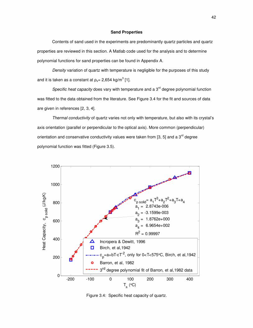
42
Sand Properties
Contents of sand used in the experiments are predominantly quartz particles and quartz
properties are reviewed in this section. A Matlab code used for the analysis and to determine
polynomial functions for sand properties can be found in Appendix A.
Density variation of quartz with temperature is negligible for the purposes of this study
and it is taken as a constant at ρs= 2,654 kg/m3 [1].
Specific heat capacity does vary with temperature and a 3rd
degree polynomial function
was fitted to the data obtained from the literature. See Figure 3.4 for the fit and sources of data
are given in references [2, 3, 4].
Thermal conductivity of quartz varies not only with temperature, but also with its crystal’s
axis orientation (parallel or perpendicular to the optical axis). More common (perpendicular)
orientation and conservative conductivity values were taken from [3, 5] and a 3rd
degree
polynomial function was fitted (Figure 3.5).
Figure 3.4: Specific heat capacity of quartz.
-200 -100 0 100 200 300 4000
200
400
600
800
1000
1200
Ts (°C)
Heat
Capacity,
cp s
olid
(J/k
g ⋅K
)
Incropera & Dewitt, 1996
Birch, et al,1942
cp=a+bT-cT-2, only for 0<T<575°C, Birch, et al,1942
Barron, et al, 1982
3rd degree polynomial fit of Barron, et al,1982 data
cp solid
= a1T3+a
2T2+a
3T+a
4
a1 = 2.8743e-006
a2 = -3.1599e-003
a3 = 1.8762e+000
a4 = 6.9654e+002
R2 = 0.99997
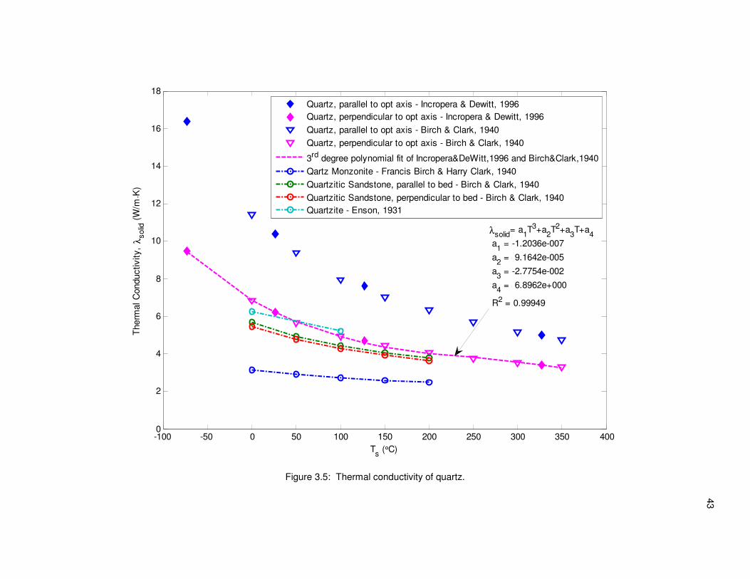
43
Figure 3.5: Thermal conductivity of quartz.
-100 -50 0 50 100 150 200 250 300 350 4000
2
4
6
8
10
12
14
16
18
Ts (°C)
Therm
al C
onductivity,
λsolid
(W
/m⋅K
)
Quartz, parallel to opt axis - Incropera & Dewitt, 1996
Quartz, perpendicular to opt axis - Incropera & Dewitt, 1996
Quartz, parallel to opt axis - Birch & Clark, 1940
Quartz, perpendicular to opt axis - Birch & Clark, 1940
3rd degree polynomial fit of Incropera&DeWitt,1996 and Birch&Clark,1940
Qartz Monzonite - Francis Birch & Harry Clark, 1940
Quartzitic Sandstone, parallel to bed - Birch & Clark, 1940
Quartzitic Sandstone, perpendicular to bed - Birch & Clark, 1940
Quartzite - Enson, 1931
λsolid= a
1T3+a
2T2+a
3T+a
4
a1 = -1.2036e-007
a2 = 9.1642e-005
a3 = -2.7754e-002
a4 = 6.8962e+000
R2 = 0.99949
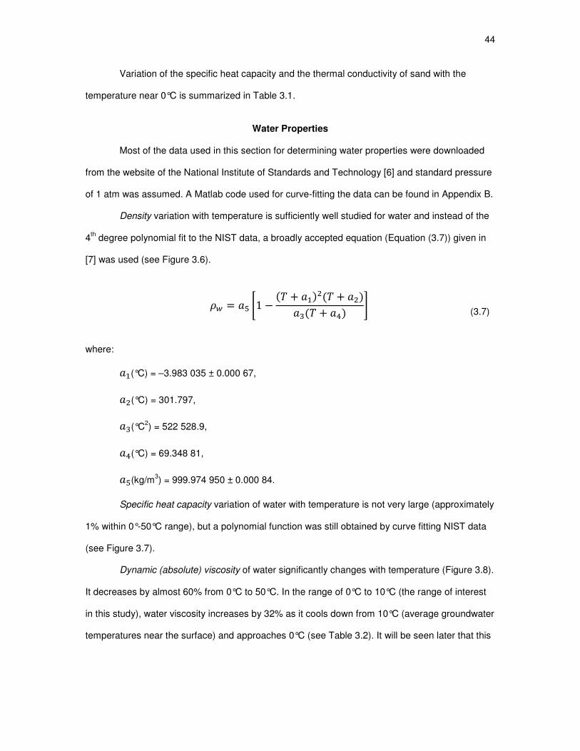
44
Variation of the specific heat capacity and the thermal conductivity of sand with the
temperature near 0°C is summarized in Table 3.1.
Water Properties
Most of the data used in this section for determining water properties were downloaded
from the website of the National Institute of Standards and Technology [6] and standard pressure
of 1 atm was assumed. A Matlab code used for curve-fitting the data can be found in Appendix B.
Density variation with temperature is sufficiently well studied for water and instead of the
4th degree polynomial fit to the NIST data, a broadly accepted equation (Equation (3.7)) given in
[7] was used (see Figure 3.6).
9 = 1 − ( + )U( + U)( + |) (3.7)
where: (°C) = –3.983 035 ± 0.000 67,
U(°C) = 301.797,
(°C2) = 522 528.9,
|(°C) = 69.348 81,
(kg/m3) = 999.974 950 ± 0.000 84.
Specific heat capacity variation of water with temperature is not very large (approximately
1% within 0°-50°C range), but a polynomial function was still obtained by curve fitting NIST data
(see Figure 3.7).
Dynamic (absolute) viscosity of water significantly changes with temperature (Figure 3.8).
It decreases by almost 60% from 0°C to 50°C. In the range of 0°C to 10°C (the range of interest
in this study), water viscosity increases by 32% as it cools down from 10°C (average groundwater
temperatures near the surface) and approaches 0°C (see Table 3.2). It will be seen later that this

45
Table 3.1: Variation of sand properties with temperature.
T (°C) cp (J/kg·K) λ (W/m·K)
50 783 5.71
10 715 6.57
0 697 6.83
-10 677 7.11
-50 594 8.49
Change from 50°C to 0°C: -11.0% 19.6%
Change from 10°C to 0°C: -2.6% 4.0%
Change from 0°C to -10°C: -2.7% 4.1%
Change from 0°C to -50°C: -14.7% 24.4%
Figure 3.6: Water density variation with temperature.
0 5 10 15 20 25 30 35 40 45 50988
990
992
994
996
998
1000
T (°C)
ρ (
kg/m
3)
NIST data points
4th degree polynomial fit
Empirical eq. from journal Metrologia, 2001, 38, pp301-309
ρw ater = a
1T4+a
2T3+a
3T2+a
4T+a
5
a1 = -3.4671e-007
a2 = 6.7777e-005
a3 = -8.5411e-003
a4 = 6.4701e-002
a5 = 9.9985e+002
R2 = 1.00000Metrologia, 2001:ρw ater
= a5[1-(T+a
1)2(T+a
2)/(a
3(T+a
4))]
a1 = -3.983035
a2 = 301.797
a3 = 522528.9
a4 = 69.34881
a5 = 999.974950

46
Figure 3.7: Water specific heat capacity variation with temperature.
0 5 10 15 20 25 30 35 40 45 50
4.175
4.18
4.185
4.19
4.195
4.2
4.205
4.21
4.215
4.22
T (°C)
cp (
kJ/k
g ⋅K
)
NIST data points
4th degree polynomial fit
cp = a
1T4+a
2T3+a
3T2+a
4T+a
5
a1 = 9.8933e-009
a2 = -1.5591e-006
a3 = 1.0407e-004
a4 = -3.2972e-003
a5 = 4.2192e+000
R2 = 0.99998

47
Figure 3.8: Water dynamic (absolute) viscosity variation with temperature.
Table 3.2: Variation of water properties with temperature.
T (°C) ρ (kg/m3) cp (J/kg·K) λ (W/m·K) µ (Pa·s) β (m
3/K)
0.01 999.9 4220 0.563 1.93E-03 -7.05E-05
10 999.7 4195 0.582 1.47E-03 8.41E-05
50 988.1 4178 0.646 7.81E-04 4.51E-04
Change from 10°C to 0.01°C: 0.01% 0.6% -3% 32% -184%
Change from 50°C to 0.01°C: 1.20% 1.0% -13% 148% -116%
0 5 10 15 20 25 30 35 40 45 500.4
0.6
0.8
1
1.2
1.4
1.6
1.8x 10
-3
T (°C)
µ (
Pa⋅s
)
NIST data points
4th degree polynomial fit
Empirical eq. from www.Wikipedia.org
µ = a1T4+a
2T3+a
3T2+a
4T+a
5
a1 = 1.2422e-010
a2 = -1.9966e-008
a3 = 1.3996e-006
a4 = -6.0393e-005
a5 = 1.7888e-003
R2 = 1.00000

48
increase is one of the main contributing factors in the damping of natural convection near freezing
temperatures in the studied porous media.
Thermal conductivity variation of water with temperature is also noticeable. Within the
range of 0°C to 50°C, conductivity increases with temperature by approximately 15% (Figure 3.9
and Table 3.2). A 4th degree polynomial function was also fitted to the NIST data.
Thermal expansion coefficient of water was calculated based on the NIST density data
and using Equation (3.8):
3 = − 19 dX9X eT (3.8)
As it can be seen from Figure 3.10, 3 also varies significantly with temperature. In the
10 degree interval from 0°C to 10°C, its value doubles (see Table 3.2).
Table 3.2 summarizes the above discussion and shows the magnitudes of water property
variances with temperature:
Ice Properties
Thermal property variations of ice with temperature are shown in Figure 3.11, Figure 3.12
and Figure 3.13, which are based on the data obtained from [8, 9]. A Matlab code for curve-fitting
can be found in Appendix C.
As it can be seen in Figure 3.11, the density of ice, after a big initial drop during phase
change from water to ice, slowly increases with lowering temperature, but its variation with
temperature is very weak. It changes only by 0.16% from 0°C to -10°C and by 0.74% from 0°C to
-50°C (Table 3.3). Variation of other ice properties, namely, specific heat capacity (Figure 3.12)
and thermal conductivity (Figure 3.13), are also not very large in the temperature range of interest
for this study. However, they reach -3.6% and 5.0% from 0°C to -10°C for specific heat capacity
and thermal conductivity, respectively (Table 3.3).

49
Figure 3.9: Water thermal conductivity variation with temperature.
0 5 10 15 20 25 30 35 40 45 50
0.57
0.58
0.59
0.6
0.61
0.62
0.63
0.64
0.65
T (°C)
λ (
W/m
⋅K)
NIST data points
4th degree polynomial fit
λw ater = a
1T4+a
2T3+a
3T2+a
4T+a
5
a1 = 1.1942e-009
a2 = -2.0865e-007
a3 = 2.6531e-006
a4 = 1.8900e-003
a5 = 5.6108e-001
R2 = 1.00000

50
Figure 3.10: Water thermal expansion coefficient variation with temperature.
0 5 10 15 20 25 30 35 40 45 50-1
0
1
2
3
4
5
6x 10
-4
T (°C)
β (
1/K
)
Points based on Metrologia 2001 empirical eq. for ρ
4th degree polynomial fit
βw ater = a
1T4+a
2T3+a
3T2+a
4T+a
5
a1 = -1.9992e-011
a2 = 3.4724e-009
a3 = -2.7200e-007
a4 = 1.7933e-005
a5 = -6.7470e-005
R2 = 1.00000

51
Figure 3.11: Ice density variation with temperature.
-50 -45 -40 -35 -30 -25 -20 -15 -10 -5 0916
917
918
919
920
921
922
923
924
T (°C)
ρic
e (
kg/m
3)
CRC Handbook data points
3rd degree polynomial fit (T in °C)
ρice= a
1T3+a
2T2+a
3T+a
4
a1 = 7.6944e-007
a2 = -1.7506e-004
a3 = -1.4600e-001
a4 = 9.1673e+002
R2 = 0.99998

52
Figure 3.12: Ice specific heat capacity variation with temperature.
-50 -45 -40 -35 -30 -25 -20 -15 -10 -5 01700
1750
1800
1850
1900
1950
2000
2050
2100
T (°C)
Cp ic
e (
J/k
g ⋅K
)
CRC Handbook data data points
3rd degree polynomial fit (T in °C)
Cp ice
= a1T3+a
2T2+a
3T+a
4
a1 = 1.3642e-005
a2 = 5.4463e-003
a3 = 7.5938e+000
a4 = 2.0988e+003
R2 = 0.99995

53
Figure 3.13: Ice thermal conductivity variation with temperature.
Table 3.3: Variation of ice properties with temperature.
T (°C) ρ (kg/m3) cp (J/kg·K) λ (W/m·K)
0 916.7 2099 2.16
-10 918.2 2023 2.26
-50 923.5 1731 2.77
Change from 0°C to -10°C: 0.16% -3.6% 5.0%
Change from 0°C to -50°C: 0.74% -17.5% 28.5%
-50 -45 -40 -35 -30 -25 -20 -15 -10 -5 02
2.1
2.2
2.3
2.4
2.5
2.6
2.7
2.8
T (°C)
λic
e (
W/m
⋅K)
CRC Handbook data data points
3rd degree polynomial fit (T in °C)
λice= a
1T3+a
2T2+a
3T+a
4
a1 = -2.3838e-007
a2 = 2.4879e-005
a3 = -1.0440e-002
a4 = 2.1576e+000
R2 = 0.99998
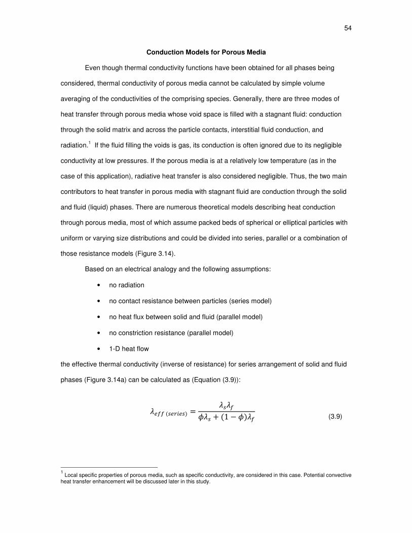
54
Conduction Models for Porous Media
Even though thermal conductivity functions have been obtained for all phases being
considered, thermal conductivity of porous media cannot be calculated by simple volume
averaging of the conductivities of the comprising species. Generally, there are three modes of
heat transfer through porous media whose void space is filled with a stagnant fluid: conduction
through the solid matrix and across the particle contacts, interstitial fluid conduction, and
radiation.1 If the fluid filling the voids is gas, its conduction is often ignored due to its negligible
conductivity at low pressures. If the porous media is at a relatively low temperature (as in the
case of this application), radiative heat transfer is also considered negligible. Thus, the two main
contributors to heat transfer in porous media with stagnant fluid are conduction through the solid
and fluid (liquid) phases. There are numerous theoretical models describing heat conduction
through porous media, most of which assume packed beds of spherical or elliptical particles with
uniform or varying size distributions and could be divided into series, parallel or a combination of
those resistance models (Figure 3.14).
Based on an electrical analogy and the following assumptions:
• no radiation
• no contact resistance between particles (series model)
• no heat flux between solid and fluid (parallel model)
• no constriction resistance (parallel model)
• 1-D heat flow
the effective thermal conductivity (inverse of resistance) for series arrangement of solid and fluid
phases (Figure 3.14a) can be calculated as (Equation (3.9)):
6NN(I\MI) = 6I6N6I + (1 − )6N (3.9)
1 Local specific properties of porous media, such as specific conductivity, are considered in this case. Potential convective
heat transfer enhancement will be discussed later in this study.

55
(a) (b) (c)
Figure 3.14: Conduction models: (a) series, (b) parallel and (c) 3-element resistor (conductor)
[10, 11].
where, 6NN is the effective conductivity of porous media, is porosity, and 6I is the
conductivity of solid and 6N of fluid phases. Similarly, the parallel arrangement (Figure 3.14b)
can be modeled as Equation (3.10):
6NN(Tp\pHHH) = 6N + (1 − )6I (3.10)
The series model yields the minimum expected thermal conductivity (6I\MI in Figure
3.15), whereas the parallel model gives an approximate upper bound for the effective conductivity
of a given porous media (6Tp\pHHH in Figure 3.15).
Other thermal conductivity models for porous media encountered in literature include
combinations of series and parallel models [10, 11, 12], which consider three parallel channels of
heat conduction; one consisting of fluid alone, second – solid alone, and the third channel
consisting of fluid and solid in series (Figure 3.14c). A comparison of the various models
accounting for a mixed conduction mode is shown in Figure 3.15. The equation describing this
mixed mode of conduction is given below (Equation (3.11)):
6NN(I T) = 6I6N6I(1 − ) + 6N + 6I + 6N (3.11)
q
solid (1-Φ)
fluid (Φ)
q
solid (1-Φ) fluid (Φ)
q
fluid (Φ)
solid (1-Φ)

56
Figure 3.15: Thermal conductivity models for porous media (water-saturated sand at 20°C).
0 0.1 0.2 0.3 0.4 0.5 0.6 0.7 0.8 0.9 10
1
2
3
4
5
6
7
Porosity, φ
Eff
ective T
herm
al C
onductivity,
λeff
(W
/m⋅K
)
λseries→
← λparallel
λs+p→
← λgeo mean
← λmin+max
λschumann→
←λspherical
← λellipsoidal
←λkrupiczka← λveinberg
λexp f ine ave→ ← λexp coarse ave
Series Resistance
Parallel Resistance = Volumetric Average: λeff= φλf
+(1-φ)λs
Series+Parallel (Kimura,1957; Woodside & Messmer,1961)
Geometric Mean (Lichteneker,1926; Asaad,1955)
Power Law (n=0.4) of Min&Max Cond. (Chaudhary & Bhandari,1968)
Schumann & Voss,1934
Random Spherical Particles (Maxwell,1873; Eucken,1932)
Random Ellipsoidal Particles (de Vries,1952)
Krupiczka,1967 (valid only for φ = 0.215 - 0.476 range)
Veinberg,1967
Exp. Values: λexp fine ave= 2.09 W/m⋅K, φexp f ine
= 0.38
Exp. Values: λexp coarse ave= 2.05 W/m⋅K, φexp coarse
= 0.4

57
where , and are coefficients and + + = 1. Some researchers using this model
assumed no direct conduction through the solid, = 0, and the following coefficients: = ., = (1 − )/. This conduction model is shown by 6I T in Figure 3.15.
A geometric mean model (Equation (3.12)) proposed by Lichteneker [13] and later by
Asaad [14] is shown as 6LJpG in Figure 3.15.
6NN(LJpG) = 6N¡6I¢¡ (3.12)
A power law combination (Equation (3.13), 6JMG Jpq in Figure 3.15) of the maximum
(parallel) and minimum (series) thermal conductivities was proposed by Chaudhary and Bhandari
[15, 16].
6NN(JMG Jpq) = 6JpqG6JMG¢G (3.13)
where ! is a weighting factor of distribution of phases in the medium. Namely, the !-th fraction
of the porous medium is assumed to be distributed according to the parallel (maximum
conductivity) model and the (1 − !)-th fraction is assumed to be distributed according to the
series (minimum conductivity) model. !’s value is obtained by the best-fit technique of
experimental values [16].
Schumann and Voss [17] derived their model (Equations (3.14), (3.15), (3.16), 6IslJpGG in Figure 3.15) based on the assumptions of point contact between spherical solid
grains and their uneven size and packing method:
6NN(IslJpGG) = 6N + (1 − )% (3.14)
where: % = 6N6I6N + B(6N − 6I) £1 + B(1 + B)(6N − 6I)6N + B(6N − 6I) ln 6N(1 + B)6IB ¦ (3.15)
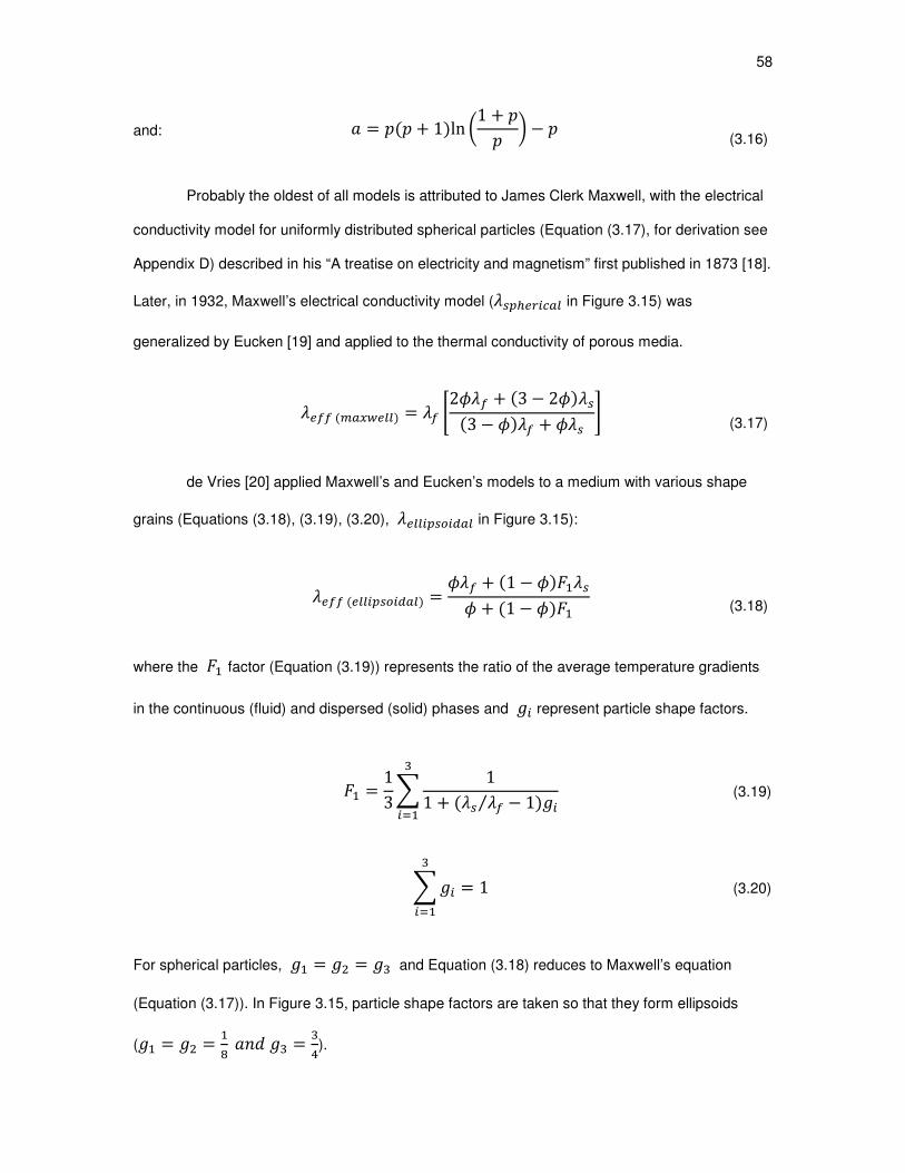
58
and: = B(B + 1)ln g1 + BB h − B (3.16)
Probably the oldest of all models is attributed to James Clerk Maxwell, with the electrical
conductivity model for uniformly distributed spherical particles (Equation (3.17), for derivation see
Appendix D) described in his “A treatise on electricity and magnetism” first published in 1873 [18].
Later, in 1932, Maxwell’s electrical conductivity model (6ITs\MpH in Figure 3.15) was
generalized by Eucken [19] and applied to the thermal conductivity of porous media.
6NN(JpqHH) = 6N 26N + (3 − 2)6I(3 − )6N + 6I (3.17)
de Vries [20] applied Maxwell’s and Eucken’s models to a medium with various shape
grains (Equations (3.18), (3.19), (3.20), 6HHMTILM+pH in Figure 3.15):
6NN(HHMTILM+pH) = 6N + (1 − )6I + (1 − ) (3.18)
where the factor (Equation (3.19)) represents the ratio of the average temperature gradients
in the continuous (fluid) and dispersed (solid) phases and M represent particle shape factors.
= 13u 11 + (6I 6N⁄ − 1)MM (3.19)
uMM = 1 (3.20)
For spherical particles, = U = and Equation (3.18) reduces to Maxwell’s equation
(Equation (3.17)). In Figure 3.15, particle shape factors are taken so that they form ellipsoids
( = U = ! = |).

59
Krupiczka’s [21] model (Equations (3.21), (3.22), 6¨\lTM]¨p in Figure 3.15) is based on
a rigorous mathematical solution for heat transfer in square packed cylinders and cubic packed
spheres, correlated with experimental data:
6NN(¨\lTM]¨p) = 6N 6I6N© ªHL«¬®
(3.21)
where: = 0.280 − 0.757@c() and ¯ = −0.057 (3.22)
Krupiczka’s correlation is valid only for a restricted region of porosity, = 0.215 − 0.476.
There are other more complex models developed by a number of researchers [22-27, 32,
33] not reviewed here. Most of the models noted above and presented in Figure 3.15 describe
thermal conductivity with reasonable accuracy in the range of interest (Φ = 0.35 – 0.45) of the
studied system of water-saturated sand. For the purposes of this dissertation, the power law
combination of min and max conductivities (Equation (3.13), Chaudhary & Bhandari, 1968) was
selected for its simplicity, adequate accuracy and the ability of fine-tuning with a weighting factor
(currently selected at n = 0.4 for a better fit of the experimental data). A Matlab code for the
analysis of conductivity models presented in this section and shown in Figure 3.15 can be seen in
Appendix E.
Verification of Selected Conduction Model
To verify the selected conduction model, experimental measurements of thermal
conductivity of water-saturated porous media were performed. The Transient Line Source Method
[29, 31] was chosen for the experimental measurements. The physical model behind this method
is injection of heat (%& ) from a line source with constant power per unit length for a specified
duration (-, see Figure 3.16) in the undisturbed porous media with uniform initial temperature
(M) and observing the speed of its dissipation.

60
Figure 3.16: Heat injection time-profile in undisturbed porous media for measurement of its
thermal conductivity.
The solution for the above-mentioned method is based on temperature (or pressure)
build-up and draw-down theory [28] and the constant linear heat source method [29, 31], and
temperature distribution (', -) in porous media is provided with Equation (3.23) [28]:
(', -) − M = %&4ℎp\r6TJ @! g- + -U-U h (3.23)
where, ±&|²sm³´ coefficient on the RHS of the above equation represents a slope, ,
(Equation (3.24)) in temperature vs. @! µr« r¶r¶ · plot for a point near the line source of heat
0 100 200 300 400 500 6000
5
10
15
20
25
30
35
40
45
50
t (sec)
Q (
W)
← Heat injection stopped after t1
← t1 → |→ t
2
Heat injection profile, (Heat = Voltage2 / Resistance)

61
(' ≈ 0), after a few seconds from turning off a heat source. In the given experiments, the slope
was determined after disregarding the first 30 seconds of measurements. The detailed
procedures and recommendations on conducting the Transient Line Source Method
measurements of conductivity in a porous medium are reviewed in [29, 30, 31]. The approximate
location of evaluating the slope is shown in Figure 3.17 and Figure 3.18 with an arrow in front of
the average effective conductivity values.
= %&4ℎp\r6TJ (3.24)
In the above equation (Equation (3.24)), ℎp\r is the length of electrical heating cartridge,
6TJ is the thermal conductivity of the measured porous material and %& is the heat rate of the
cartridge, which can be calculated knowing its resistance (() and RMS voltage (0) from
Equation (3.25):
%& = 0U( (3.25)
Thus, calculating a slope, , of the temperature versus the natural log of (- + -U)/-
from the experimental plots (Figure 3.17 and Figure 3.18), the thermal conductivity of the porous
media can be determined (Equation (3.26)):
6TJ = %&4ℎp\r (3.26)
As theory applies to a perfect line heat source, length-to-diameter ratio of the heating
cartridge should be infinitely large. Beck [29] suggests using a heating probe with a length-to-
diameter ratio of about 50, but points out that “this can often be halved without significant errors
creeping in” measurements. According to Blackwell’s analytical derivations [30], if the heating
probe’s length-to-diameter ratio is 30 or more, the experimental measurements will yield

62
Figure 3.17: Thermal conductivity measurements of water-saturated fine sand (Mar 26-27, 2011).
Each line represents a separate experiment. Experiments with the same heat injection times have
the same color.
0 0.5 1 1.5 2 2.5 3 3.5 4 4.5 5 5.520
21
22
23
24
25
26
27
28
29
30
ln((t+∆t)/t)
T (
°C)
Heat injected for 60 sec
Heat injected for 120 sec
Heat injected for 180 sec
← λaverage = 2.09 W/m⋅K
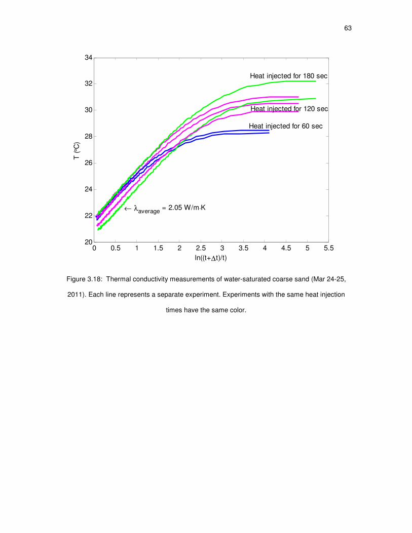
63
Figure 3.18: Thermal conductivity measurements of water-saturated coarse sand (Mar 24-25,
2011). Each line represents a separate experiment. Experiments with the same heat injection
times have the same color.
0 0.5 1 1.5 2 2.5 3 3.5 4 4.5 5 5.520
22
24
26
28
30
32
34
ln((t+∆t)/t)
T (
°C)
Heat injected for 60 sec
Heat injected for 120 sec
Heat injected for 180 sec
← λaverage = 2.05 W/m⋅K

64
negligible errors. The heating cartridge used in the present study had a length of 33 cm and
diameter of 6.3 mm, resulting in a length-to-diameter ratio of 52.4, satisfying the above-mentioned
conditions. The experimental apparatus for the effective thermal conductivity measurements of
porous media are shown in Figure 3.19.
After measuring the electrical resistance of the heating cartridge (R = 80.1 Ω), the RMS
voltage of the AC power supplied through a variable voltage transformer (V = 50 Volts), and
running several experiments for water-saturated sand packs, the average thermal conductivities
were found to be 6TJ,NMG= 2.09 W/m·K and 6TJ,Lp\I = 2.05 W/m·K for fine and coarse
sand packs, respectively (Figure 3.17 and Figure 3.18).
Both average conductivity values are within the expected range of water-saturated sand
pack for given porosities (see Figure 3.15), confirming a reasonable choice of the selected
effective conductivity model (Equation (3.13)).
(a)
(b)
Figure 3.19: Experimental setup for thermal conductivity measurements of water-saturated sand:
(a) centrally positioned heating cartridge and type-T thermocouple, (b) coarse sand and data
logger.
Heating cartridge
Thermocouple
65
References
[1] Birch, F., Schairer, J. F., Spicer, H. C., 1942, “Handbook of Physical Constants,” Geological Society of America, Special Papers, 36, p. 12.
[2] Birch, F., Schairer, J. F., Spicer, H. C., 1942, “Handbook of Physical Constants,”
Geological Society of America, Special Papers, 36, p. 224. [3] Incropera, F. P., DeWitt, D. P., 1996, ”Fundamentals of Heat and Mass Transfer,” John
Wiley & Sons, New York, 4th ed.
[4] Barron, T. H. K., Collins, J. F., Smith, T. W., White, G. K., 1982, “Thermal Expansion,
Gruneisen Functions and Static Lattice Properties of Quartz,” Journal of Physics C: Solid State Physics, 15, pp. 4311-4326.
[5] Birch, F., Clark, H., 1940, “The Thermal Conductivity of Rocks and Its Dependence upon
Temperature and Composition,” American Journal of Science, pp. 529-558. [6] Lemmon, E. W., McLinden, M. O., Friend, D. G., "Thermophysical Properties of Fluid
Systems," in NIST Chemistry WebBook, NIST Standard Reference Database Number 69, Eds. Linstrom, P. J. and Mallard, W.G., National Institute of Standards and Technology, Gaithersburg, MD, 20899, http://webbook.nist.gov (Accessed on Nov 5, 2009).
[7] Tanaka, M., Girard, G., Davis, R., Peuto, A., Bignell, N., 2001, “Recommended Table for
the Density of Water between 0°C and 40°C Based on Recent Experimental Reports,” J. Metrologia, 38, pp. 301-309.
[8] Haynes, W. M., 2010-2011, “CRC Handbook of Chemistry and Physics”, 91
st ed., CRC
Press, Boca Raton, pp. 6-12. [9] Website: http://www.engineeringtoolbox.com/ice-thermal-properties-d_576.html
(Accessed on Sep 6, 2010). [10] Wyllie, M. R. J., Southwick, P. F., 1954, “An Experimental Investigation of the S.P. and
Resistivity Phenomena in Dirty Sands,” J. of Petroleum Technology, 6(2), pp. 44-57. [11] Kimura, M., 1957, Kagaku Kōgaku Kyōkai (Journal of Chemical Engineering of Japan),
21, p. 472. [12] Woodside, W., Messmer, J. H., 1961, “Thermal Conductivity of Porous Media. I.
Unconsolidated Sands,” J. of Applied Physics, 32(9), pp. 1688-1699. [13] Lichtenecker, K., 1926, Physik, 27, p. 115. [14] Asaad, Y., 1955, “A Study of Thermal Conductivity of Fluid Bearing Porous Rocks,” PhD
thesis, University of California, Berkeley. [15] Chaudhary, D. R., Bhandari, R. C., 1968, “Heat Transfer through a Three-Phase Porous
Medium,” Brit. J. Appl. Phys (J. Phys. D.), 2(1), pp. 815-817. [16] Chaudhary, D. R., Bhandari, R. C., 1969, “Thermal Conductivity of Two-Phase Porous
Materials: Dry Soils,” Brit. J. Appl. Phys (J. Phys. D.), 2(2), pp. 609-610. [17] Schumann, T. E. W., Voss, V., 1934, ”Heat Flow through Granulated Material,” Fuel,
13(8), pp. 249-256.
66
[18] Maxwell, J. C., 1873, “A Treatise on Electricity and Magnetism,” Clarendon Press, Oxford, 1st ed., 1, pp. 365-366.
[19] Eucken, A., 1932, Forsch. Gebiete Ingenieurw, B3, VDI- Forschungsheft, p. 353. [20] de Vries, D. A., 1952, Mededelingen van de Landbouwhogeschol te Wageningen, pp. 1-
73. [21] Krupiczka, R., 1967, ”Analysis of Thermal Conductivity in Granular Materials,”
International Chemical Engineering, 7(1), pp. 122-144. [22] Tien, Nayak, 1978, “A Statistical Thermodynamic Theory for Coordination – Number
Distribution and Effective Thermal Conductivity of Random Packed Beds,” Int’l J. of Heat and Mass Transfer, 21, pp. 669-676.
[23] Kunii, D., Smith, J. M., 1960, “Heat Transfer Characteristics of Porous Rocks,” J. Amer.
Inst. Chem. Engrs., 6(1), p. 71. [24] Gonzo, E. E., 2002, “Estimating Correlations for the Effective Thermal Conductivity of
Granular Materials,” Chemical Engineering Journal, 90, pp. 299-302. [25] Argento, C., Bouvard, D., 1996, “Modeling the Effective Thermal Conductivity of Random
Packing of Spheres through Densification,” Int. J. Heat Mass Transfer, 39(7), pp. 1343-1350.
[26] Lu, S., Ren, T., Gong, Y., Horton, R., 2007, ”An Improved Model for Predicting Soil
Thermal Conductivity from Water Content at Room Temperature,” Soil Sci. Soc. Am. J., 71(1), pp. 8-14.
[27] Tavman, I. H., 1996, “Effective Thermal Conductivity of Granular Porous Materials,” Int.
Comm. Heat Mass Transfer, 23(2), pp. 169-176. [28] Udell, K. S., 2006, Lecture notes for course MEEN 7960 “Multiphase Transport in Porous
Media,” University of Utah, Department of Mechanical Engineering, Salt Lake City, UT, USA.
[29] Beck, A. E., 1988, "Methods for Determining Thermal Conductivity and Thermal
Diffusivity," in Handbook of Terrestrial Heat-Flow Density Determination, Edited by Haenel, R., Rybach, L., Stegena, L., Kluwer, Dordrecht, pp. 87-124.
[30] Blackwell, J. H., 1956, “The Axial-Flow Error in the Thermal-Conductivity Probe”, Can. J.
Phys. 34, pp. 412-417. [31] IEEE Guide for Soil Thermal Resistivity Measurements, IEEE Std 442-1981 (Reaffirmed
1996), p. 7. [32] Veinberg, A. K., 1967, "Permeability, Electrical Conductivity, Dielectric Constant and
Thermal Conductivity of a Medium with Spherical and Ellipsoidal Inclusions," Soviet Physics - Doklady, A translation of the ’Physics Section’ of the Proceedings of the Academy of Sciences of the USSR, 11, pp. 593-595.
[33] Weaver,J. A., Viskanta, R., 1986, "Freezing of Liquid-Saturated Porous Media," J. of
Heat Transfer, Transactions of the ASME, 108, pp. 654-659.

4. EXPERIMENTAL SETUP AND PROCEDURES
In this chapter, the experimental apparatus designed and built in the Sustainable Energy
Lab on the Department of Mechanical Engineering of the University of Utah is presented and the
experimental procedures are described.
Experimental Apparatus
For the experimental studies presented in this work, a thermosiphon was designed and
built using 11.4 cm (4.5 in) outer diameter and 130 cm (51 in) long, schedule 10, alloy 6063-T6
aluminum pipe. The bottom of the pipe was sealed with a welded plate, and a flange supporting
an air-to-liquid heat exchanger and instrumentation was welded on the top (Figure 4.1). An array
of 36 type K thermocouples was installed on a wooden frame attached to the side wall of the
thermosiphon (Figure 4.1a, Figure 4.2c). Wood was used to minimize heat transfer enhancement
by conduction in the frame. The thermosiphon was charged with the working fluid (R-134a
refrigerant) and placed in a thermally insulated 90 Gallon cylindrical tank made of polyethylene
(Figure 4.1b). The top and bottom of the tank were insulated with double layers of extruded
polystyrene foam board (with R-value of 10) and two layers of fiberglass insulation (with R-value
of 13) were wrapped around the side walls of the tank, and secured with a reflective sheet of zinc-
plated steel. The insulation was used to approximate the adiabatic boundaries of the section of
the cylindrical cell of a thermal storage with a thermosiphon in the center.
As mobility of the apparatus was desired, a steel cart was built (welded) and the
experimental apparatus was placed on it. The cart provided the ability to easily move the tank
with the thermosiphon out of the building for heat extraction experiments using ambient cold air in
winter and roll it back inside the building for heat injection (air conditioning) mode experiments in
the lab.

68
(a) (b)
Figure 4.1: Experimental apparatus: (a) thermocouple array attached to thermosiphon wall, (b)
thermosiphon inside a thermally insulated tank filled with water-saturated sand.
For the experimental data acquisition, a 20 channel Graphtec GL800 data logger [1] with
an additional 20 channel extension, providing a total of 40 temperature acquisition channels, was
selected. For reversibility of the thermosiphon operation and delivering the working fluid to the
heat exchanger mounted on the top of the apparatus, a small (30 W) electromagnetic oscillating
piston pump [2] with a suction filter was installed on the bottom inside the thermosiphon (Figure
4.2a). Aluminum mesh was placed inside the thermosiphon to provide uniform distribution of the
working fluid to the internal walls and increase the surface area of evaporation (Figure 4.2b).
A centrifugal fan, commonly used in HVAC industry, was placed on the cart next to the
insulated tank and supplied the ambient air through the air duct to the heat exchanger mounted
on the top of the thermosiphon (see Figure 4.1b and Figure 4.3b).
Welded flange supporting
instrumentation
Data logger
Thermocouple array
Thermosiphon
Heat exchanger
Air duct
Insulated tank

69
(a)
(b)
(c)
Figure 4.2: Experimental apparatus - assembly details: (a) pump and filter assembly, (b)
aluminum screen/mesh, (c) thermocouple array.
Oscillating piston pump
Inlet filter

70
(a) (b)
Figure 4.3: Experimental apparatus - orifice flow meter details on the air duct: (a) orifice and
pressure outlet locations, (b) U-tube manometer filled with water.
For the measurement of the air flow rate supplied to the heat exchanger, an orifice
restriction (as shown in Figure 2.4) was installed inside the air duct (Figure 4.3a). The pressure
difference across the orifice was measured with a water U-tube manometer (Figure 4.3b).
Experimental Procedures
Using the above-described apparatus, a number of experiments were run using hot water
for calibrating the tank insulation and determining the heat losses to the ambient. The overall heat
transfer coefficient of the insulated tank was determined as: UAtank ≈ 1.59 W/°C. Cold water and
ice/water mix was used for testing the active (pump-assisted) mode of operation of the
thermosiphon. Later, water was replaced with the water-saturated fine grain sand, and finally,
with the coarse sand pack. The height of the water-saturated sand pack filling the tank was
approximately 1.14 m. As mentioned before, the experiments were run mostly in winter, taking
Pressure outlet after the orifice
Location of the orifice restriction
Pressure outlet before
the orifice
Water level in the U-tube manometer
Fan housing

71
advantage of cold weather for freezing the water in the porous media in the tank, and then
cooling the warm lab air by injecting its heat into the tank, thus thawing the frozen water in the
porous medium. During the experiments, the temperature data from thermocouples, placed in the
porous medium and at the inlet and outlet of the heat exchanger, were recorded by the data
logger with 1 min intervals. The air fan provided a constant air flow which was periodically
monitored with a water column displacement height in a U-tube manometer measuring a pressure
drop across the orifice meter in the air duct.
Heat extraction experiments were run before heat injection. The initial temperature
distribution in the porous medium before the heat extraction was uniform. The tank with the
thermal storage medium was rolled outside and heat was extracted and dissipated in the ambient
air. The thermosiphon was operated in passive mode with the air heat exchanger acting as a
condenser for the working fluid. After freezing (or cooling, depending on the ambient air
temperatures) the porous medium, the experiment was stopped and the temperature data were
downloaded from the data logger. The tank was rolled back to the lab and the heat injection
experiment was started. The liquid pump on the bottom of the thermosiphon was turned on,
reversing the direction of the flow in the system and delivering the cold working fluid to the air
heat exchanger, which operated as an evaporator in this case. After warming up the thermal
storage to within a couple of degrees of the ambient lab air temperature, the heat injection
experiment was stopped and the temperature data were downloaded from the data logger.
These heat extraction-injection cycles were repeated a number of times during the
winters of 2008-2009 and 2009-2010. The detailed experimental results and discussion is
provided in the following chapter.

72
References
[1] Data Logger Manual: Graphtec midi LOGGER GL800, Graphtec America, Inc. http://www.graphtecusa.com/
[2] Electromagnetic pump ELS-50 30W, Gotec SA. http://www.gotec.ch
5. EXPERIMENTAL RESULTS
After building the experimental apparatus, 22 experiments were run. 11 of those
experiments were run with water, 7 experiments with fine grain and 4 experiments with coarse
grain sand packs. The experiments lasted from several hours to several days and were run
during the period 2008-2010. Water experiments were used for calibration of the thermal
insulation (determining heat losses/gains) of the tank and for testing the operating principles of
the reversible thermosiphon. Thus, the detailed results of water experiments are not discussed
here. Of interest for this work are heat transfer modes in water-saturated porous media and,
respectively, the data from the most characteristic experiments (see Table 5.1) with heat
injection/extraction into/from water-saturated sand packs illustrating the different modes of heat
transfer is presented in this chapter.
As Rayleigh number characterizes the heat transfer mode in the porous medium, the
uncertainties in Ra values, which are calculated based on the experimental measurements of
other parameters, are of interest. The following section is devoted to the uncertainty analysis of
the Rayleigh number.
Uncertainty Analysis
For estimating the uncertainty in Rayleigh number, URa, the uncertainties of measured
temperature, thermosiphon length, permeability, thermal expansion coefficient of water, thermal
diffusivity of porous media, water viscosity, and other parameters, as follows below, have to be
determined first.
The uncertainty in thermosiphon length. The thermosiphon length inserted in the
porous medium, L=1.14 m, was measured with a tape meter with the least division of 1 mm and
the measurement could have been made to the nearest millimeter with a probable error of

74
Table 5.1: Summary of data on characteristic experiments.
Run ID Start Date
Duration (hours)
Porosity ¸ Permeability
k (m2)
Regime Ramax Convection Corresp. Figures
Fine Sand -
Freezing
Dec 4, 2009
185 0.38 1.93•10-10
Passive - Extraction
2.2 No
Figure 5.8
Figure 5.12
Figure 5.16
Figure 5.26
Figure 5.32
Fine Sand -
Freezing
Dec 26, 2009
170 0.38 1.93•10-10
Passive - Extraction
2.5 No
Figure 5.9
Figure 5.13
Figure 5.17
Figure 5.27
Figure 5.33
Coarse Sand - Cooling
Feb 7, 2010
160 0.40 2.03•10-9
Passive - Extraction
118 Strong
Figure 5.10
Figure 5.14
Figure 5.18
Figure 5.28
Figure 5.34
Coarse Sand - Cooling
Feb 19, 2010
140 0.40 2.03•10-9
Passive - Extraction
53 Moderate
Figure 5.11
Figure 5.15
Figure 5.19
Figure 5.29
Figure 5.35
Fine Sand -
Air Cond.
Jan 2, 2010
45 0.38 1.93•10-10
Active - Injection
2.7 Weak
Figure 5.20
Figure 5.22
Figure 5.24
Figure 5.30
Figure 5.37
Coarse Sand -
Air Cond.
Feb 25, 2010
46 0.40 2.03•10-9
Active - Injection
34 Moderate
Figure 5.21
Figure 5.23
Figure 5.25
Figure 5.31
Figure 5.37
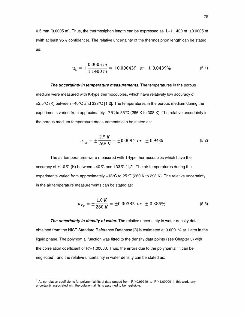
75
0.5 mm (0.0005 m). Thus, the thermosiphon length can be expressed as L=1.1400 m ±0.0005 m
(with at least 95% confidence). The relative uncertainty of the thermosiphon length can be stated
as:
.¹ = ±0.00051.1400 = ±0.000439' ± 0.0439% (5.1)
The uncertainty in temperature measurements. The temperatures in the porous
medium were measured with K-type thermocouples, which have relatively low accuracy of
±2.5°C (K) between −40°C and 333°C [1,2]. The temperatures in the porous medium during the
experiments varied from approximately −7°C to 35°C (266 K to 308 K). The relative uncertainty in
the porous medium temperature measurements can be stated as:
.Fº = ± 2.5 266 = ±0.0094' ± 0.94% (5.2)
The air temperatures were measured with T-type thermocouples which have the
accuracy of ±1.0°C (K) between −40°C and 133°C [1,2]. The air temperatures during the
experiments varied from approximately −13°C to 25°C (260 K to 298 K). The relative uncertainty
in the air temperature measurements can be stated as:
.F» = ± 1.0 260 = ±0.00385' ± 0.385% (5.3)
The uncertainty in density of water. The relative uncertainty in water density data
obtained from the NIST Standard Reference Database [3] is estimated at 0.0001% at 1 atm in the
liquid phase. The polynomial function was fitted to the density data points (see Chapter 3) with
the correlation coefficient of R2=1.00000. Thus, the errors due to the polynomial fit can be
neglected1 and the relative uncertainty in water density can be stated as:
1 As correlation coefficients for polynomial fits of data ranged from R
2=0.99949 to R
2=1.00000 in this work, any
uncertainty associated with the polynomial fits is assumed to be negligible.

76
.f = ±0.000001' ± 0.0001% (5.4)
The uncertainty in dynamic viscosity of water. The relative uncertainty in the data of
the dynamic viscosity of water obtained from the NIST Standard Reference Database [3], which
itself was based on IAPWS formulation [4], is estimated at 0.17% in 0°C-20°C range. The
polynomial function was fitted to the dynamic viscosity data points (see Chapter 3) with the
correlation coefficient of R2=1.00000. Thus, the errors due to the polynomial fit can be neglected
and the relative uncertainty in dynamic viscosity of water can be stated as:
.¼ = ±0.0017' ± 0.17% (5.5)
The uncertainty in kinematic viscosity of water. The uncertainty in kinematic viscosity
of water, uν, depends on the relative uncertainties in water density, uρ, and dynamic viscosity of
water, uµ. As kinematic viscosity, 8, is defined as:
8 = ¼f , (5.6)
the relative uncertainty in kinematic viscosity of water, uν, can be expressed as:
., = ±g78 X8X7.¼hU + g98 X8X9 .fhUU
= ±g78 19 .¼hU + g98 g− 79Uh .fhUU
= ±½.¼U + w−.fxU¾U = ±¿0.0017U + (−0.000001)UÀU = ±0.0017' ± 0.17%
(5.7)

77
The uncertainty in thermal conductivity of water. The data of the thermal conductivity
of water were obtained from the NIST Standard Reference Database [3], which itself was based
on [5], with the higher uncertainties near 0°C. At T=1°C, it is estimated as 6 =563 ±11 W/m·K
[5]. Thus, the relative uncertainty of the thermal conductivity of water, ., can be stated as:
. = ± 11Á/ · 563Á/ · = ±0.0195' ± 1.95% (5.8)
The uncertainty in heat capacity of water. According to [3], the relative uncertainty in
isobaric heat capacity of water is:
.T = ±0.1% (5.9)
The uncertainty in porosity. The porosity measurements were conducted using a 2,000
ml graduated beaker with the least division of 100 ml. The measurement could have been made
to the nearest 100 ml with a probable error of 50 ml (0.00005 m3). In the case of fine sand, the
total volume of the porous medium was measured as Vtotal fine = 1880 ml ± 50ml and its
saturating water as Vwater = 710 ml ± 50ml, yielding the relative uncertainty in the measured
porosity of fine sand:
.¡®Â = ±g− 50@1880@hU + g 50@710@hUU
= ±0.0753' ± 7.53%
(5.10)
In the case of coarse sand, the total volume of the porous medium was measured as
Vtotal coarse = 1790 ml ± 50ml and its saturating water as Vwater = 710 ml ± 50ml, yielding the
relative uncertainty in the measured porosity of coarse sand:

78
.¡Ãm = ±g− 50@1790@hU + g 50@710@hUU
= ±0.0758' ± 7.58%
(5.11)
The uncertainty in density of ice. The density data for ice were obtained from the CRC
Handbook of Chemistry and Physics [6], which was based on the equation of state for hexagonal
ice (ice Ih) given in [7], and its relative uncertainty, .fM , is estimated at 0.04% in the 268–273 K
range [7]:
.fM = ±0.04% (5.12)
The uncertainty in heat capacity of ice. The heat capacity data for ice were also
obtained from [6] and according to [7], its relative uncertainty,.M , below 273 K is estimated as:
.M = ±4% (5.13)
The uncertainty in thermal conductivity of ice. The thermal conductivity data for ice
were obtained from [6], which was based on the formulation given in [8], and its uncertainty,.M, is estimated at 5% in the 40–273 K range [7]:
.M = ±5% (5.14)
The uncertainty in density of sand (quartz). The constant value for density of quartz
was taken from [9], but no uncertainty was reported. Thus, zero uncertainty for the density of
sand is used here:
.fI = ±0% (5.15)

79
The uncertainty in heat capacity of sand (quartz). The uncertainty in heat capacity
data for quartz [10] is estimated as 0.2% in 20-273 K interval and as 1% at higher than 273 K
temperatures. A higher value of 1% relative uncertainty is used in this work:
.I = ±1% (5.16)
The uncertainty in thermal conductivity of sand (quartz). The thermal conductivity
data for quartz were taken from [11] and [12], but no uncertainty values were reported in either of
the sources. The thermal conductivity data in [12] were adopted from [13], which reports
maximum uncertainty in thermal conductivity of quartz at <7%. Thus, 7% value for the relative
uncertainty in thermal conductivity of quartz,.I, is used here:
.I = ±7% (5.17)
The uncertainties in air properties. The data for air properties were obtained from [14].
As uncertainties are not reported by the above-mentioned source, no uncertainty in air property
data was used in this work.
The uncertainty in permeability measurements. For the experimental measurement of
permeabilities, 5 runs were performed for each, fine and coarse sand packs. The results are
shown in Table 5.2.
Table 5.2: Permeability measurement results for coarse and fine sand packs.
Experimental
run
Measured permeability of
sand pack
N kcoarse (m2) kfine (m
2)
1 2.088E-09 2.016E-10
2 2.132E-09 1.955E-10
3 2.007E-09 1.923E-10
4 1.983E-09 1.889E-10
5 1.953E-09 1.854E-10
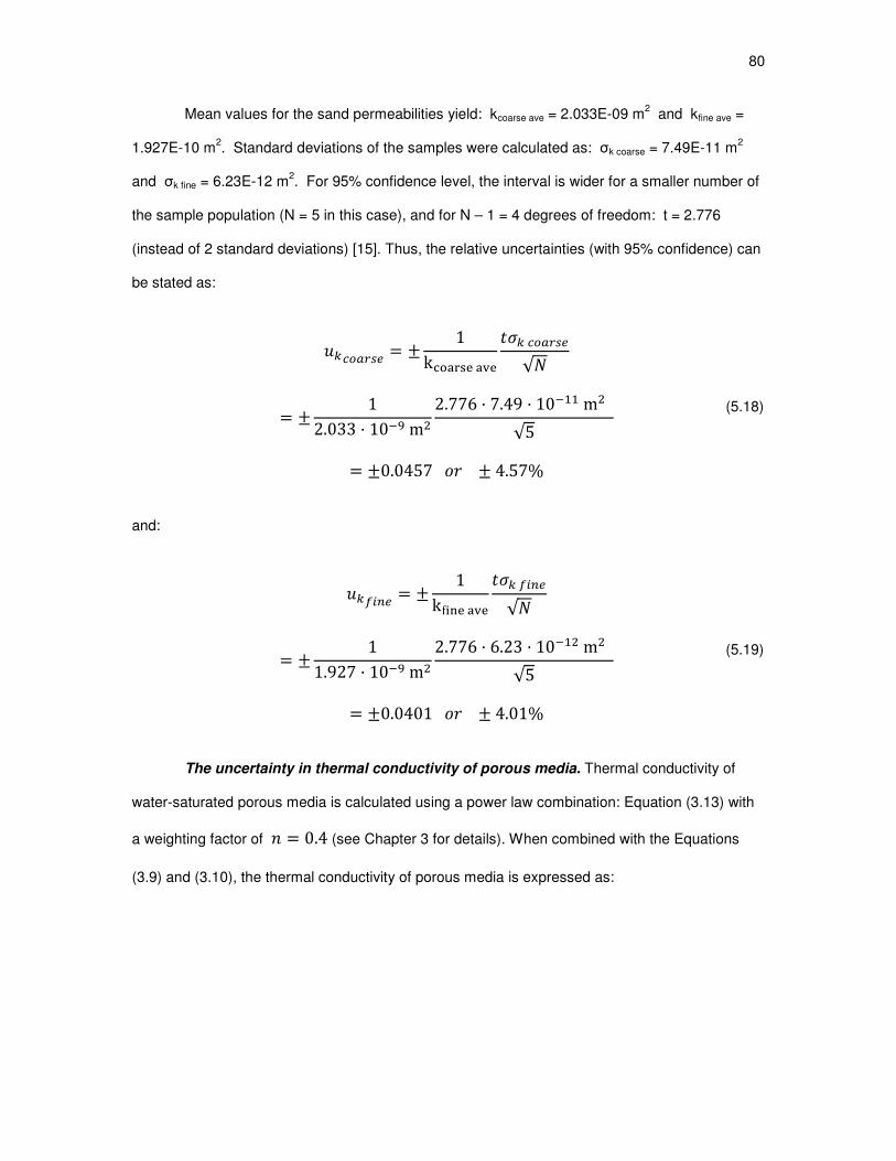
80
Mean values for the sand permeabilities yield: kcoarse ave = 2.033E-09 m2 and kfine ave =
1.927E-10 m2. Standard deviations of the samples were calculated as: σk coarse = 7.49E-11 m
2
and σk fine = 6.23E-12 m2. For 95% confidence level, the interval is wider for a smaller number of
the sample population (N = 5 in this case), and for N – 1 = 4 degrees of freedom: t = 2.776
(instead of 2 standard deviations) [15]. Thus, the relative uncertainties (with 95% confidence) can
be stated as:
.¨Lp\I = ± 1kÅÆÇÈÉÊÇËÊ -:¨Lp\I√Í
= ± 12.033 · 10¢ÎmU 2.776 · 7.49 · 10¢mU√5
= ±0.0457' ± 4.57%
(5.18)
and:
.¨NMG = ± 1kÐÑÒÊÇËÊ -:¨NMG√Í
= ± 11.927 · 10¢ÎmU 2.776 · 6.23 · 10¢UmU√5
= ±0.0401' ± 4.01%
(5.19)
The uncertainty in thermal conductivity of porous media. Thermal conductivity of
water-saturated porous media is calculated using a power law combination: Equation (3.13) with
a weighting factor of ! = 0.4 (see Chapter 3 for details). When combined with the Equations
(3.9) and (3.10), the thermal conductivity of porous media is expressed as:

81
6TJ = v6N + (1 − )6IyG · 6I6N6I + (1 − )6N¢G
= v6N + (1 − )6IyUG¢ · v6I6Ny¢G
= v6N + (1 − )6Iy¢c.U · v6I6Nyc. (5.20)
The relative uncertainty in thermal conductivity of porous media can be stated as:
.TJ = ±Ó 6TJ X6TJX .¡U + 6I6TJ X6TJX6I .U + 6N6TJ X6TJX6N .®UÔ
U (5.21)
where:
X6TJX = −0.2w6N − 6Ixw6I6Nxc.w6N + (1 − )6Ix.U
= − 0.2w6N − 6Ixw6N + (1 − )6Ix · 6TJ
X6TJX6I = 0.66Nw6I6Nxc.|(6N + (1 − )6I)c.U − 0.2(1 − )w6I6Nxc.(6N + (1 − )6I).U = 0.66I − 0.2(1 − )(6N + (1 − )6I) · 6TJ
X6TJX6N = 0.66Iw6I6Nxc.|w6N + (1 − )6Ixc.U − 0.2w6I6Nxc.w6N + (1 − )6Ix.U = 0.66N − 0.2w6N + (1 − )6Ix · 6TJ
(5.22)
After substituting (3.22) into Equation (3.21), the relative uncertainty in thermal
conductivity of porous media can be expressed in the following form:

82
.TJ = ±Õ− 0.2w6N − 6Ixw6N + (1 − )6Ix · .¡U
+ Ö0.6 − 0.2(1 − )6I(6N + (1 − )6I) · .×U
+ Ø0.6 − 0.26Nw6N + (1 − )6Ix · .®ÙUÚU
(5.23)
When uncertainties in thermal conductivity of water-saturated porous media are
evaluated near the water-freezing temperatures (0°C-20°C), they yield the following results (also
see Figure 5.1):
.TJNMG = ±0.0319' ± 3.19% (5.24)
and for the coarse sand pack:
.TJLp\I = ±0.0322' ± 3.22% (5.25)
The uncertainty in volumetric heat capacity of porous media. Volumetric heat
capacity (mean thermal capacitance) of water-saturated porous media is calculated using
Equation (5.26):
9WWW = 9T + (1 − )9II (5.26)
The relative uncertainty in volumetric heat capacity of water-saturated porous media can
be stated then as:

83
Figure 5.1: Relative uncertainties in thermal conductivities of water-saturated fine and coarse
sand packs.
0 2 4 6 8 10 12 14 16 18 203.185
3.19
3.195
3.2
3.205
3.21
3.215
3.22
3.225
T (°C)
Rela
tive u
ncert
ain
ty,
%
uλ pm, f ine, ave
= 3.19 %
uλ pm, coarse, ave
= 3.22 %

84
.fWWWW = ±Óg 9WWW X9WWWX .¡hU + g99WWW X9WWWX9 .fÛhU + T9WWW X9WWWXT .ÛU
+ g9I9WWW X9WWWX9I .fhU + gI9WWW X9WWWXI .hUU
(5.27)
where:
X9WWWX = 9T − 9II X9WWWX9 = T
X9WWWXT = 9
X9WWWX9I = (1 − )I X9WWWXI = (1 − )9I
(5.28)
After substituting (5.28) into Equation (5.27) and taking into account that no uncertainty
for the density of quartz was reported, thus .fI = 0 assumed, the relative uncertainty in
volumetric heat capacity of water-saturated porous media can be expressed in the following form:
.fWWWW = ±Ów9T − 9IIx9WWW .¡U + g9T9WWW .fÛhU
+ g9T9WWW .ÛhU + (1 − )9II9WWW .UU
(5.29)

85
When uncertainties in volumetric heat capacity of water-saturated porous media are
evaluated near water-freezing temperatures (see Figure 5.2), maximum uncertainties can be
seen when temperature approaches 0°C. Thus, using a conservative approach, the relative
uncertainties in volumetric heat capacity of water-saturated porous media can be stated as:
.fWWWWNMG = ±0.0250' ± 2.50% (5.30)
and for the coarse sand pack:
.fWWWWLp\I = ±0.0260' ± 2.60% (5.31)
Figure 5.2: Relative uncertainties in volumetric heat capacity of water-saturated fine and coarse
sand packs.
0 2 4 6 8 10 12 14 16 18 202.3
2.35
2.4
2.45
2.5
2.55
2.6
2.65
2.7
T (°C)
Rela
tive u
ncert
ain
ty,
%
uρc pm, f ine, max
= 2.50 %
uρc pm, coarse, max
= 2.60 %
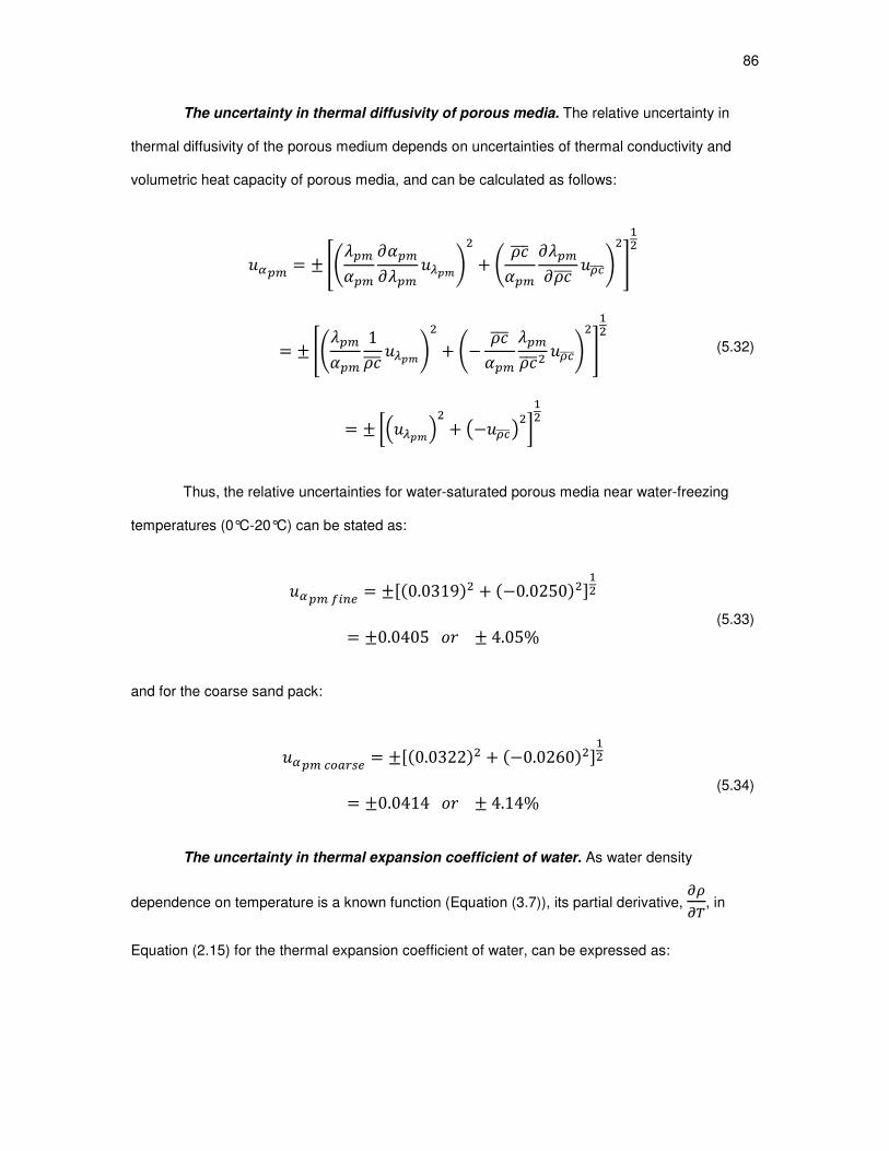
86
The uncertainty in thermal diffusivity of porous media. The relative uncertainty in
thermal diffusivity of the porous medium depends on uncertainties of thermal conductivity and
volumetric heat capacity of porous media, and can be calculated as follows:
.ÜTJ = ±Ó6TJ2TJ X2TJX6TJ .´U + 9WWW2TJ X6TJX9WWW .fWWWWUÔ
U
= ± Ó6TJ2TJ 19WWW .´U + − 9WWW2TJ 6TJ9WWWU .fWWWWUÔU
= ±Ýµ.´·U + w−.fWWWWxUÞU (5.32)
Thus, the relative uncertainties for water-saturated porous media near water-freezing
temperatures (0°C-20°C) can be stated as:
.ÜTJNMG = ±¿(0.0319)U + (−0.0250)UÀU = ±0.0405' ± 4.05%
(5.33)
and for the coarse sand pack:
.ÜTJLp\I = ±¿(0.0322)U + (−0.0260)UÀU = ±0.0414' ± 4.14%
(5.34)
The uncertainty in thermal expansion coefficient of water. As water density
dependence on temperature is a known function (Equation (3.7)), its partial derivative, EfEF, in
Equation (2.15) for the thermal expansion coefficient of water, can be expressed as:
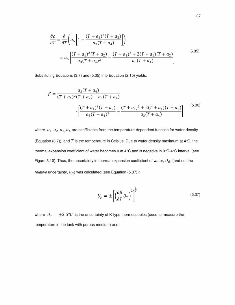
87
X9X = XX 1 − ( + )U( + U)( + |)
= ( + )U( + U)( + |)U − ( + )U + 2( + )( + U)( + |) (5.35)
Substituting Equations (3.7) and (5.35) into Equation (2.15) yields:
3 = ( + |)( + )U( + U) − ( + |)· ( + )U( + U)( + |)U − ( + )U + 2( + )( + U)( + |) (5.36)
where ,U,,| are coefficients from the temperature-dependent function for water density
(Equation (3.7)), and is the temperature in Celsius. Due to water density maximum at 4°C, the
thermal expansion coefficient of water becomes 0 at 4°C and is negative in 0°C-4°C interval (see
Figure 3.10). Thus, the uncertainty in thermal expansion coefficient of water,/ß, (and not the
relative uncertainty, .ß) was calculated (see Equation (5.37)):
/ß = ±gX3X /FhUU (5.37)
where /F = ±2.5° is the uncertainty of K-type thermocouples (used to measure the
temperature in the tank with porous medium) and:

88
X3X = àááâ( + )U + 2( + )( + U)( + |) − ( + )U( + U)( + |)U( + )U( + U)( + |) − 1 ãää
åU
− àááâ2( + )U( + U)( + |) − 2( + )U + 4( + )( + U)( + |)U + 4( + ) + 2( + U)( + |)( + )U( + U)( + |) − 1 ãää
å
(5.38)
The uncertainty in the thermal expansion coefficient of water near water-freezing
temperatures (0°C-20°C) is shown in Figure 5.3.
Figure 5.3: Uncertainty in thermal expansion coefficient of water.
0 2 4 6 8 10 12 14 16 18 202.6
2.8
3
3.2
3.4
3.6
3.8
4
4.2
4.4
4.6x 10
-5
T (°C)
Uncert
ain
ty,
Uβ (
1/ °
C)
Uβ , max
= 4.54e-005 1/°C

89
Again, with a conservative approach, the uncertainty in the thermal expansion coefficient
of water near water-freezing temperatures can be stated as:
/ß = ±4.54 · 10¢ 1° (5.39)
or using the values for /ß from Figure 5.3, the thermal expansion coefficient of water in 0°C-20°C
temperature interval is shown in Figure 5.4.
The uncertainty in Rayleigh number. As Rayleigh number in porous media is defined
by the Equation (2.24), its uncertainty, /æp, can be calculated with the Equation (5.40):
Figure 5.4: Thermal expansion coefficient of water in 0°C-20°C temperature range.
0 2 4 6 8 10 12 14 16 18 20-1.5
-1
-0.5
0
0.5
1
1.5
2
2.5x 10
-4
T (°C)
β (
1/ °
C)

90
/æp = ±ÓgX(X3 /ßhU + gX(X /¹hU + gX(X /¨hU + X(X2TJ /Ü´U
+ gX(X8 /,hU + gX(XI /FhU + gX(Xk /FçhUU
= ± ÓgX(X3 /ßhU + g X(X .¹hU + g X(X .¨hU + 2TJ X(X2TJ .Ü´U
+ g8 X(X8 .,hU + gX(XI /FhU + gX(Xk /FçhUU
(5.40)
where:
X(X3 = (I − k)2TJ8
X(X = 3(I − k)2TJ8
X(X = 3(I − k)2TJ8
X(X2TJ = −3(I − k)2TJU8
X(X8 = −3(I − k)2TJ8U
X(XI = 32TJ8
X(Xk = −32TJ8
(5.41)
Substituting partial derivatives of Ra from Equation (5.41) into Equation (5.40) yields:

91
/æp = ±Ó(I − k)2TJ8 /ßU + 3(I − k)2TJ8 .¹U
+ 3(I − k)2TJ8 .¨U + −3(I − k)2TJ8 .Ü´U
+ −3(I − k)2TJ8 .,U + 32TJ8 /FU
+ −32TJ8 /FçUU
(5.42)
or expressed in terms of Ra number:
/æp = ±g(3 /ßhU + g( /¹hU + (( · .¨)U + µ−( · .Ü´·U + (−( · .,)U+ g ((I − k)/FhU + g− ((I − k) /FçhU
U
= ±( g13 /ßhU + (.¹)U + (.¨)U + µ−.Ü´·U + (−.,)U+ g 1(I − k)/FhU + g− 1(I − k) /FçhU
U
(5.43)
It can be seen from the Equation (5.43) that the uncertainty in the Rayleigh number
depends (in addition to the uncertainties of variables in the Equation (2.24)) on the driving
temperature difference (I − k) in the Rayleigh number. The uncertainty in Ra increases with
the increase in the driving temperature difference, which yields a higher Rayleigh number even if
other variables are held constant (for the same temperature of the porous medium). The
uncertainties in Ra for = (I − k) = 5&20 in 0°C-20°C temperature range are
illustrated in Figure 5.5.

92
Figure 5.5: Uncertainty in Rayleigh numbers for = (I − k) = 5&20.
The Rayleigh number dependence on temperature with associated uncertainties for
water-saturated porous media with fine and coarse sand packs in 0°C-20°C range are shown in
Figure 5.6 and Figure 5.7, respectively.
For convenience, the uncertainties of all parameters used for the calculation of the
uncertainty in Rayleigh number are summarized in Table 5.3.
Rayleigh Numbers and Temperature Distribution in Porous Media
during Heat Extraction
Temperature plots from four experiments with heat removal, two from water-saturated
fine sand packs (Figure 5.8 and Figure 5.9) and two from coarse grain sand packs (Figure 5.10
and Figure 5.11), are presented in this section. The respective temperature isotherms in the
0 2 4 6 8 10 12 14 16 18 200
5
10
15
20
25
30
T (°C)
Uncert
ain
ty in R
a,
UR
a
URa fine
@ ∆T=5°C
URa coarse
@ ∆T=5°C
URa f ine
@ ∆T=20°C
URa coarse
@ ∆T=20°C

93
Figure 5.6: Temperature dependence of Rayleigh numbers and associated uncertainties for = (I − k) = 5&20 for the water-saturated fine sand pack.
0 2 4 6 8 10 12 14 16 18 20-4
-2
0
2
4
6
8
10
12
14
16
T (°C)
Ra
Raf ine
@ ∆T=5°C
Raf ine
@ ∆T=20°C
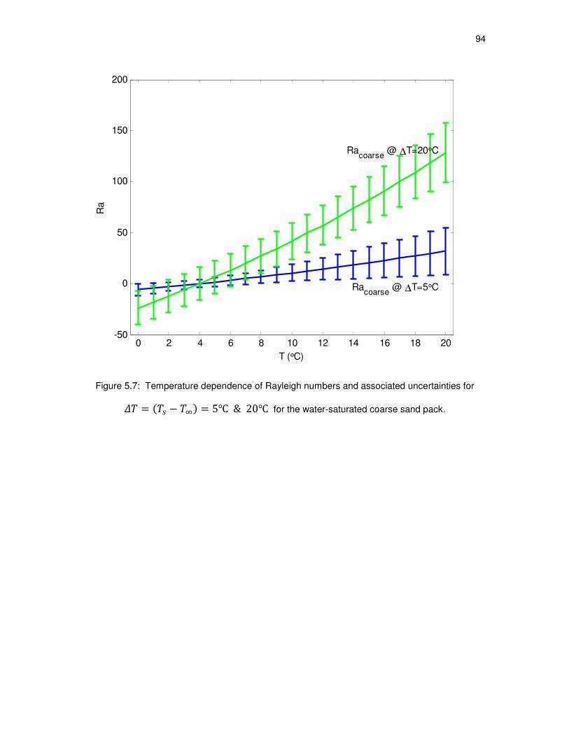
94
Figure 5.7: Temperature dependence of Rayleigh numbers and associated uncertainties for = (I − k) = 5&20 for the water-saturated coarse sand pack.
0 2 4 6 8 10 12 14 16 18 20-50
0
50
100
150
200
T (°C)
Ra
Racoarse
@ ∆T=5°C
Racoarse
@ ∆T=20°C
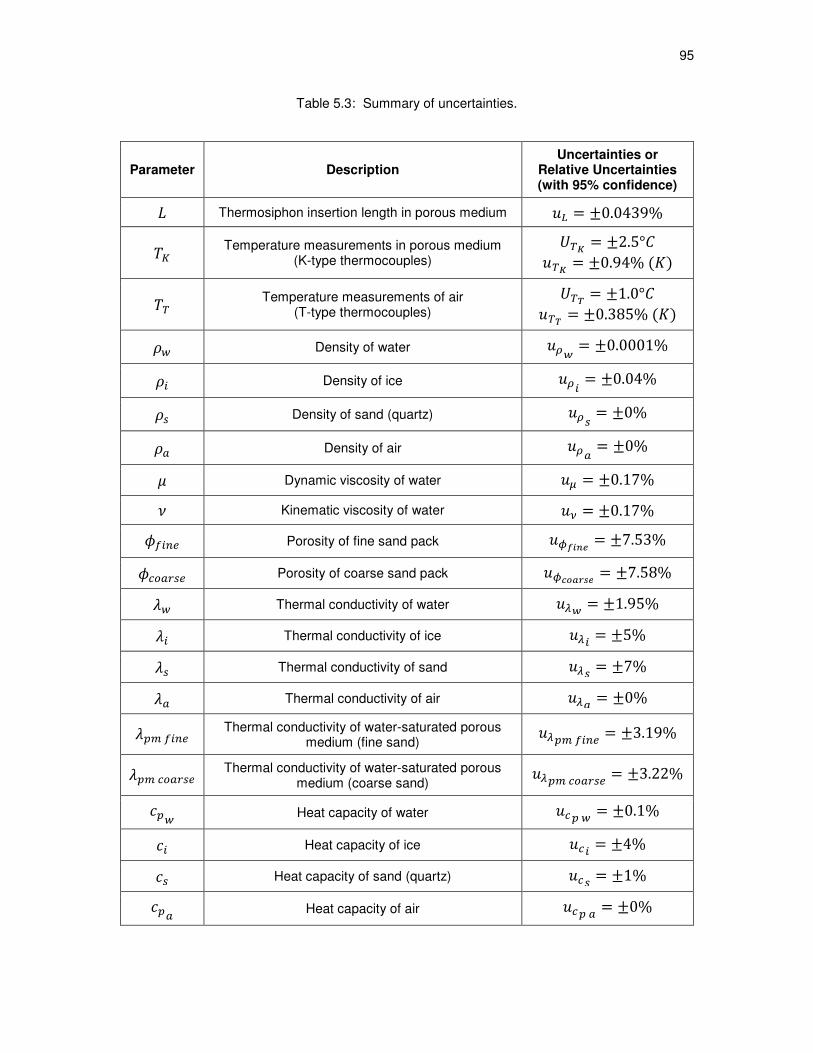
95
Table 5.3: Summary of uncertainties.
Parameter Description Uncertainties or
Relative Uncertainties (with 95% confidence) Thermosiphon insertion length in porous medium .¹ = ±0.0439%
è Temperature measurements in porous medium
(K-type thermocouples)
/Fº = ±2.5° .Fº = ±0.94%( ) F
Temperature measurements of air (T-type thermocouples)
/F» = ±1.0° .F» = ±0.385%( ) 9 Density of water .f = ±0.0001%
9M Density of ice .fM = ±0.04%
9I Density of sand (quartz) .fI = ±0%
9p Density of air .fp = ±0%
7 Dynamic viscosity of water .¼ = ±0.17% 8 Kinematic viscosity of water ., = ±0.17% NMG Porosity of fine sand pack .¡®Â = ±7.53%
Lp\I Porosity of coarse sand pack .¡Ãm = ±7.58% 6 Thermal conductivity of water . = ±1.95% 6M Thermal conductivity of ice .M = ±5% 6I Thermal conductivity of sand .I = ±7% 6p Thermal conductivity of air .p = ±0%
6TJNMG Thermal conductivity of water-saturated porous
medium (fine sand) .TJNMG = ±3.19%
6TJLp\I Thermal conductivity of water-saturated porous
medium (coarse sand) .TJLp\I = ±3.22%
T Heat capacity of water .T = ±0.1%
M Heat capacity of ice .M = ±4% I Heat capacity of sand (quartz) .I = ±1% Tp Heat capacity of air .Tp = ±0%

96
Table 5.3 continued.
Parameter Description Uncertainties or
Relative Uncertainties (with 95% confidence) NMG Permeability of fine sand pack .¨NMG = ±4.01%
Lp\I Permeability of coarse sand pack .¨Lp\I = ±4.57%
9WWWNMG Volumetric heat capacity of water-saturated fine sand pack
.fWWWWNMG = ±2.50%
9WWWLp\I Volumetric heat capacity of water-saturated coarse sand pack
.fWWWWLp\I = ±2.60%
2TJNMG Thermal diffusivity of water-saturated porous
medium (fine sand) .ÜTJNMG = ±4.05%
2TJLp\I Thermal diffusivity of water-saturated porous
medium (coarse sand) .ÜTJLp\I = ±4.14%
3 Thermal expansion coefficient of water /ß = ±4.54 · 10¢ 1°
(NMG Rayleigh number in water-saturated porous medium (fine sand)
Figure 5.5 & Figure 5.6
(Lp\I Rayleigh number in water-saturated porous medium (coarse sand)
Figure 5.5 & Figure 5.7
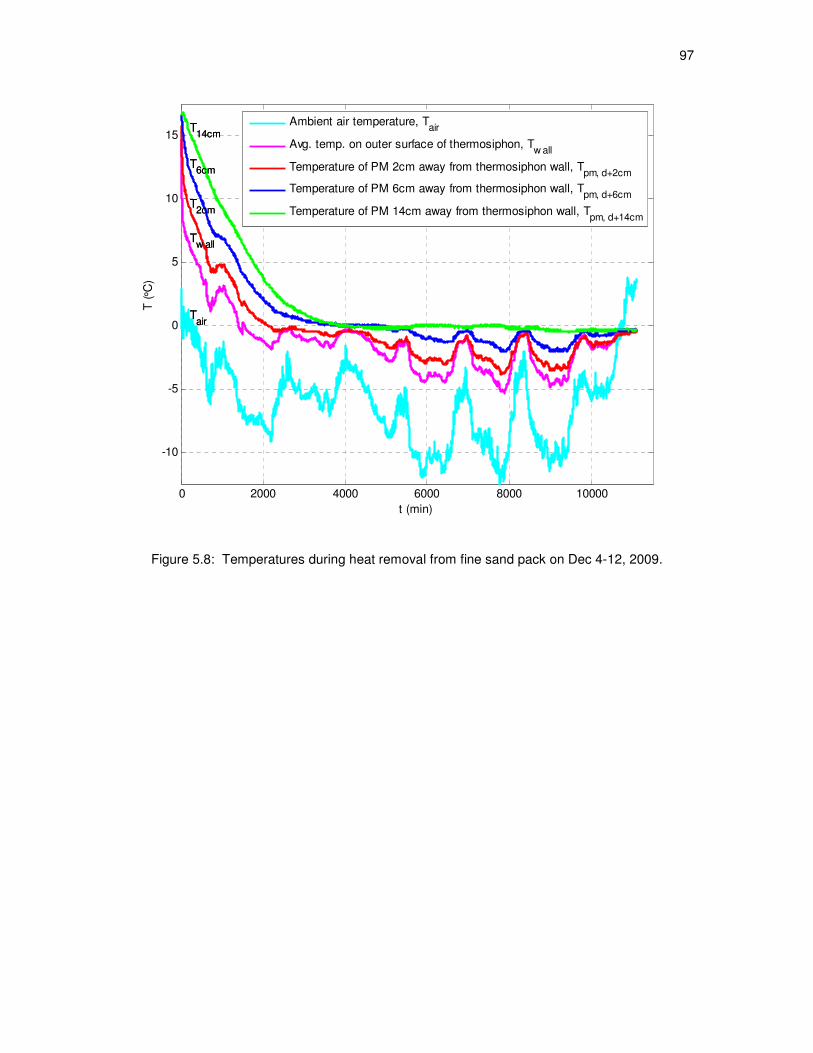
97
Figure 5.8: Temperatures during heat removal from fine sand pack on Dec 4-12, 2009.
0 2000 4000 6000 8000 10000
-10
-5
0
5
10
15
t (min)
T (°C
)
Tair
Tw all
T2cm
T6cm
T14cm
Tair
Tw all
T2cm
T6cm
T14cm
Ambient air temperature, Tair
Avg. temp. on outer surface of thermosiphon, Tw all
Temperature of PM 2cm away from thermosiphon wall, Tpm, d+2cm
Temperature of PM 6cm away from thermosiphon wall, Tpm, d+6cm
Temperature of PM 14cm away from thermosiphon wall, Tpm, d+14cm

98
Figure 5.9: Temperatures during heat removal from fine sand on Dec 26, 2009 - Jan 2, 2010.
0 1000 2000 3000 4000 5000 6000 7000 8000 9000 10000-10
-5
0
5
10
15
t (min)
T (
°C)
Tair
Tw all
T2cm
T6cm
T14cm
Ambient air temperature, Tair
Avg. temp. on outer surface of thermosiphon, Tw all
Temperature of PM 2cm away from thermosiphon wall, Tpm, d+2cm
Temperature of PM 6cm away from thermosiphon wall, Tpm, d+6cm
Temperature of PM 14cm away from thermosiphon wall, Tpm, d+14cm

99
Figure 5.10: Temperatures during heat removal from coarse sand pack on Feb 7-14, 2010.
0 1000 2000 3000 4000 5000 6000 7000 8000 9000 10000-5
0
5
10
15
20
25
30
35
t (min)
T (
°C)
Tair
Tw all
T2cm
T6cm
T14cm
Ambient air temperature, Tair
Avg. temp. on outer surface of thermosiphon, Tw all
Temperature of PM 2cm away from thermosiphon wall, Tpm, d+2cm
Temperature of PM 6cm away from thermosiphon wall, Tpm, d+6cm
Temperature of PM 14cm away from thermosiphon wall, Tpm, d+14cm

100
Figure 5.11: Temperatures during heat removal from coarse sand pack on Feb 19-25, 2010.
0 1000 2000 3000 4000 5000 6000 7000 8000 9000
-5
0
5
10
15
20
t (min)
T (
°C)
Tair
Tw all
T2cm
T6cm
T14cm
Ambient air temperature, Tair
Avg. temp. on outer surface of thermosiphon, Tw all
Temperature of PM 2cm away from thermosiphon wall, Tpm, d+2cm
Temperature of PM 6cm away from thermosiphon wall, Tpm, d+6cm
Temperature of PM 14cm away from thermosiphon wall, Tpm, d+14cm

101
porous media for various time snapshots are presented in Figure 5.12 through Figure 5.15 and
the Rayleigh number plots are shown in Figure 5.16 through Figure 5.19. The cooling of the sand
packs was due to exposure of the thermosiphon heat exchanger, operating as a condenser in this
case, to outside air in winter.
During both fine sand heat extraction experiments, a varying degree of freezing of water
in porous media was achieved (as allowed by the low ambient air temperatures), which can be
inferred from the temperatures of the sand/water mixture dropping well below 0°C at different
distances from the thermosiphon wall (Figure 5.8 and Figure 5.9). The thermocouples measuring
temperature distribution in the radial direction (Twall, T2cm, T6cm, T14cm) were positioned at
approximately midpoint of the tank height, at 50 cm from the bottom. The freezing front
propagation can be observed from the location of 0°C isotherm in the snapshots of the isotherms
in Figure 5.12 and Figure 5.13. Almost vertical shapes (except a noticeable heat loss from the top
surface of the tank, due to nonairtight top insulation, visible in the first snapshot in Figure 5.12a)
of the isotherms indicate that the heat transfer direction was essentially horizontal and no natural
convection was present. This is supported by the respective Rayleigh number plots shown in
Figure 5.16 and Figure 5.17. The Rayleigh numbers for both experiments start at approximately
2.5 and drop to 0 as temperature of the water in the porous matrix decreases. In order for natural
convection cells to develop in porous media, the Rayleigh number should be in the range of 10-
40 or above [16, 17, 18], which was not the case for those two experiments.
The interesting point is the negative value of the Rayleigh number in 1400-3300 min
interval in Figure 5.16 and 1000-2800 min interval in Figure 5.17. As the porous medium cools
down during heat extraction, and its temperature passes the water density inversion point (4°C),
thermal expansion coefficient, β, changes its sign and becomes negative below 4°C (see Figure
3.10). The negative sign of β in 0°C - 4°C interval causes the Rayleigh number to take a negative
sign as well (see the definition of Rayleigh number, Equation (2.24)). This indicates that near the
thermosiphon wall, as water cools down below 4°C, convective cell rotation direction could also
change, as colder than 4°C water elements have lower density and tend to move upwards due to
buoyancy force instead of sinking downward. The above-described phenomenon would yield two

102
(a) (b) (c)
Figure 5.12: Characteristic isotherms during heat removal from fine sand pack on Dec 4-12,
2009 at 0.5 h, 36 h and 150 h from the beginning of the experiment.
0 0.1 0.2 0.30
0.2
0.4
0.6
0.8
1
9
9
10
10
11 12
13
14 15
16
17
Fine Sand - Freezing2009/12/4 21:49:29t = 0.5 h, Ra = 2.0
Tair in
= -0.2°C, Tair out
= 1.7°C
r (m)
z (
m)
0 0.1 0.2 0.30
0.2
0.4
0.6
0.8
1
-2
-2-1
0
1
2
3
Fine Sand - Freezing2009/12/6 09:19:29t = 36.0 h, Ra = -0.3
Tair in
= -8.6°C, Tair out
= -8.1°C
r (m)
z (
m)
0 0.1 0.2 0.30
0.2
0.4
0.6
0.8
1
-5-4 -3 -2 -1
Fine Sand - Freezing2009/12/11 03:19:29t = 150.0 h, Ra = -0.8
Tair in
= -11.2°C, Tair out
= -11.0°C
r (m)
z (
m)

103
(a) (b) (c)
Figure 5.13: Characteristic isotherms during heat removal from fine sand pack on Dec 26, 2009 -
Jan 2, 2010 at 0.5 h, 36 h and 62 h from the beginning of the experiment.
0 0.1 0.2 0.30
0.2
0.4
0.6
0.8
1
8
9
10
11
12
13
14
15
16
17
Fine Sand - Freezing2009/12/26 13:44:08
t = 0.5 h, Ra = 2.3T
air in= -2.7°C, T
air out= 0.1°C
r (m)
z (
m)
0 0.1 0.2 0.30
0.2
0.4
0.6
0.8
1
-3-2
-2-1
0
1
2
Fine Sand - Freezing2009/12/28 01:14:08t = 36.0 h, Ra = -0.3
Tair in
= -8.7°C, Tair out
= -8.4°C
r (m)
z (
m)
0 0.1 0.2 0.30
0.2
0.4
0.6
0.8
1
-3-2
-1
0
0
Fine Sand - Freezing2009/12/29 03:14:08t = 62.0 h, Ra = -0.3
Tair in
= -8.3°C, Tair out
= -8.2°C
r (m)
z (
m)
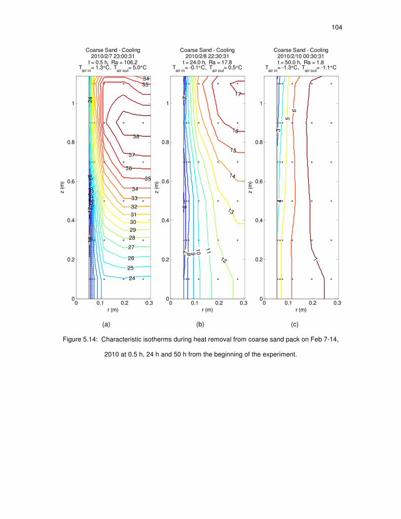
104
(a) (b) (c)
Figure 5.14: Characteristic isotherms during heat removal from coarse sand pack on Feb 7-14,
2010 at 0.5 h, 24 h and 50 h from the beginning of the experiment.
0 0.1 0.2 0.30
0.2
0.4
0.6
0.8
1
17
18
19
20
21
22
23
24
24
25
26
27
28
29
30
31
32
33
34
3435
35
36
37
38
Coarse Sand - Cooling2010/2/7 23:00:31
t = 0.5 h, Ra = 106.2T
air in= 1.3°C, T
air out= 5.0°C
r (m)
z (
m)
0 0.1 0.2 0.30
0.2
0.4
0.6
0.8
1
67
7 8
91
0
11
12
13
14
15
16
17
Coarse Sand - Cooling2010/2/8 22:30:31
t = 24.0 h, Ra = 17.8T
air in= -0.1°C, T
air out= 0.5°C
r (m)
z (
m)
0 0.1 0.2 0.30
0.2
0.4
0.6
0.8
1
34
56
7
Coarse Sand - Cooling2010/2/10 00:30:31t = 50.0 h, Ra = 1.8
Tair in
= -1.3°C, Tair out
= -1.1°C
r (m)
z (
m)
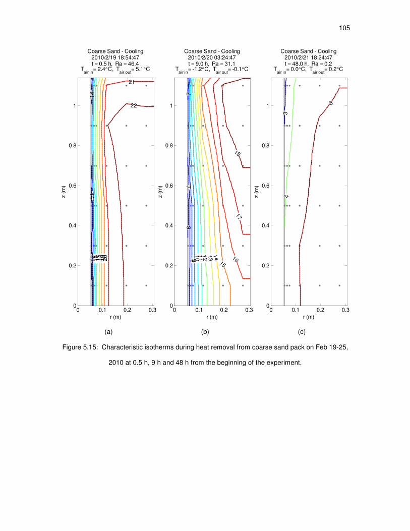
105
(a) (b) (c)
Figure 5.15: Characteristic isotherms during heat removal from coarse sand pack on Feb 19-25,
2010 at 0.5 h, 9 h and 48 h from the beginning of the experiment.
0 0.1 0.2 0.30
0.2
0.4
0.6
0.8
1
13
14
14
15
16
17
18
19
20
21
22
Coarse Sand - Cooling2010/2/19 18:54:47t = 0.5 h, Ra = 46.4
Tair in
= 2.4°C, Tair out
= 5.1°C
r (m)
z (
m)
0 0.1 0.2 0.30
0.2
0.4
0.6
0.8
1
67
7
8
91
01
112 13
14
15
16
17
18
Coarse Sand - Cooling2010/2/20 03:24:47t = 9.0 h, Ra = 31.1
Tair in
= -1.2°C, Tair out
= -0.1°C
r (m)
z (
m)
0 0.1 0.2 0.30
0.2
0.4
0.6
0.8
1
34
5
Coarse Sand - Cooling2010/2/21 18:24:47t = 48.0 h, Ra = 0.2
Tair in
= 0.0°C, Tair out
= 0.2°C
r (m)
z (
m)
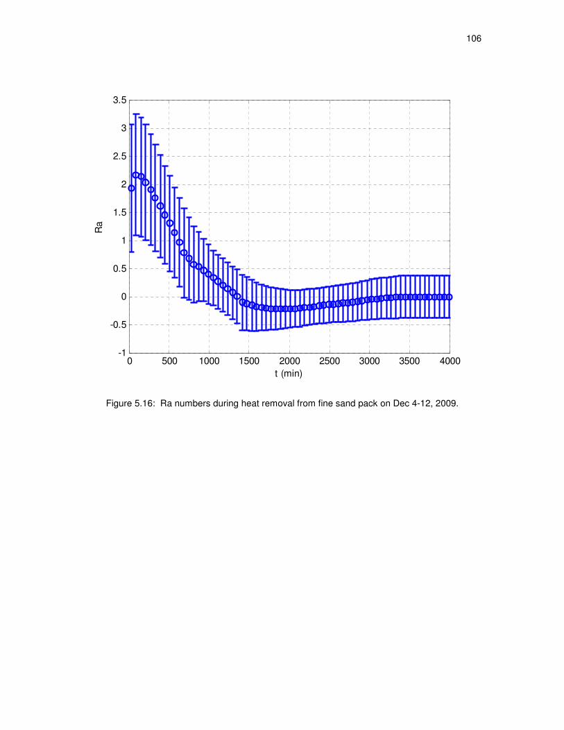
106
Figure 5.16: Ra numbers during heat removal from fine sand pack on Dec 4-12, 2009.
0 500 1000 1500 2000 2500 3000 3500 4000-1
-0.5
0
0.5
1
1.5
2
2.5
3
3.5
t (min)
Ra

107
Figure 5.17: Ra numbers during heat removal from fine sand pack on Dec 26, 2009 - Jan 2,
2010.
0 500 1000 1500 2000 2500 3000 3500 4000-1
-0.5
0
0.5
1
1.5
2
2.5
3
3.5
4
t (min)
Ra
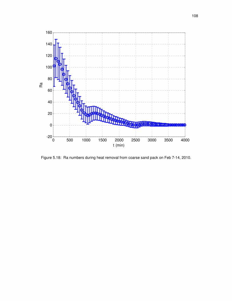
108
Figure 5.18: Ra numbers during heat removal from coarse sand pack on Feb 7-14, 2010.
0 500 1000 1500 2000 2500 3000 3500 4000-20
0
20
40
60
80
100
120
140
160
t (min)
Ra

109
Figure 5.19: Ra numbers during heat removal from coarse sand pack on Feb 19-25, 2010.
0 500 1000 1500 2000 2500 3000 3500 4000-10
0
10
20
30
40
50
60
70
80
t (min)
Ra

110
counter-rotating convective cells with the 4°C (highest density) water sinking in the middle and
water with temperature higher and lower than 4°C (lower density) moving upwards. In the
numerical simulations, this was actually modeled by FLUENT with fluid velocities on the order of
10-5
- 10-7
m/s (see Chapter 6), but its effect is unnoticeable due to high viscous forces (thus, very
low transport velocities of the fluid) at low temperatures and Ra<10.
During nighttime, when the outside air temperatures drop considerably, the thermosiphon
wall and surrounding porous medium temperatures noticeably decrease too. The closer the
location of the thermocouple in the porous medium (T2cm, T6cm, T14cm) to the thermosiphon wall
(Twall), the lower its measured temperature (see temperature oscillations following daily cycle in
Figure 5.8, Figure 5.9, Figure 5.10, Figure 5.11). As air temperature increases during the day,
heat removal rate by the thermosiphon decreases due to smaller temperature difference between
the sand pack and outside air. Thus, during daytime, heat flowing from the far-field equalizes
temperatures near the thermosiphon wall with the rest of the bulk porous medium and all
thermocouple readings approach the bulk porous medium temperature as well.
It is interesting to observe that during its passive heat extraction operation, the
thermosiphon indeed acts as a thermal diode: when ambient air temperatures increase over
those of the porous medium inside the tank, heat transfer through the thermosiphon stops and
temperatures of the porous medium near the thermosiphon walls do not increase beyond those of
the bulk medium in the tank. This can be clearly seen at the end of the experiments, as air
temperatures increase above 0°C (in Figure 5.8, Figure 5.9) or above 2°C (in Figure 5.11),
porous medium temperatures stays constant.
In heat removal experiments from the water-saturated coarse sand pack, the outside air
temperatures were not very low, barely going below 0°C (see Figure 5.10 and Figure 5.11). Thus,
freezing of water did not occur. In order to facilitate natural convection, the first coarse sand
experiment was started with a high initial temperature of the porous medium. The tank with dry
coarse sand was filled with approximately 40°C hot water and after a few minutes was rolled
outside the building to be exposed to cold ambient air. This is the reason why the porous
medium’s initial temperatures are much higher than in any other experiments presented here.
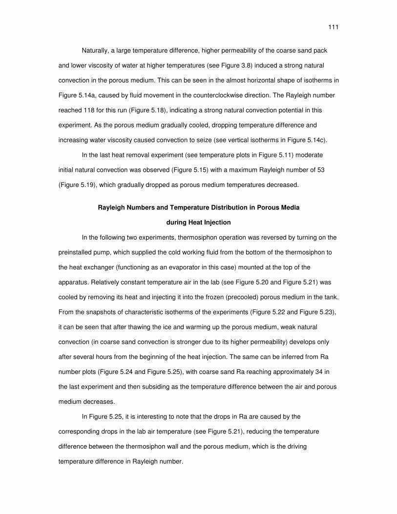
111
Naturally, a large temperature difference, higher permeability of the coarse sand pack
and lower viscosity of water at higher temperatures (see Figure 3.8) induced a strong natural
convection in the porous medium. This can be seen in the almost horizontal shape of isotherms in
Figure 5.14a, caused by fluid movement in the counterclockwise direction. The Rayleigh number
reached 118 for this run (Figure 5.18), indicating a strong natural convection potential in this
experiment. As the porous medium gradually cooled, dropping temperature difference and
increasing water viscosity caused convection to seize (see vertical isotherms in Figure 5.14c).
In the last heat removal experiment (see temperature plots in Figure 5.11) moderate
initial natural convection was observed (Figure 5.15) with a maximum Rayleigh number of 53
(Figure 5.19), which gradually dropped as porous medium temperatures decreased.
Rayleigh Numbers and Temperature Distribution in Porous Media
during Heat Injection
In the following two experiments, thermosiphon operation was reversed by turning on the
preinstalled pump, which supplied the cold working fluid from the bottom of the thermosiphon to
the heat exchanger (functioning as an evaporator in this case) mounted at the top of the
apparatus. Relatively constant temperature air in the lab (see Figure 5.20 and Figure 5.21) was
cooled by removing its heat and injecting it into the frozen (precooled) porous medium in the tank.
From the snapshots of characteristic isotherms of the experiments (Figure 5.22 and Figure 5.23),
it can be seen that after thawing the ice and warming up the porous medium, weak natural
convection (in coarse sand convection is stronger due to its higher permeability) develops only
after several hours from the beginning of the heat injection. The same can be inferred from Ra
number plots (Figure 5.24 and Figure 5.25), with coarse sand Ra reaching approximately 34 in
the last experiment and then subsiding as the temperature difference between the air and porous
medium decreases.
In Figure 5.25, it is interesting to note that the drops in Ra are caused by the
corresponding drops in the lab air temperature (see Figure 5.21), reducing the temperature
difference between the thermosiphon wall and the porous medium, which is the driving
temperature difference in Rayleigh number.

112
Figure 5.20: Temperatures during heat injection in fine sand pack on Jan 2-4, 2010.
0 500 1000 1500 2000 2500 3000-5
0
5
10
15
20
25
t (min)
T (
°C)
Tair
Tw all avg
T2cm
T6cm
T14cm
Ambient air temperature, Tair
Avg. temp. on outer surface of thermosiphon, Tw all, avg
T of PM 2cm away from thermosiphon wall, Tpm, d+2cm
T of PM 6cm away from thermosiphon wall, Tpm, d+6cm
T of PM 14cm away from thermosiphon wall, Tpm, d+14cm
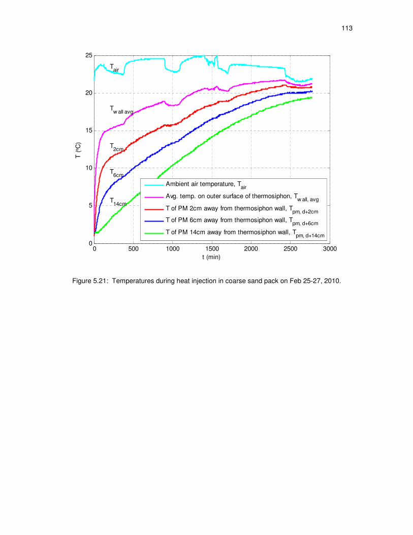
113
Figure 5.21: Temperatures during heat injection in coarse sand pack on Feb 25-27, 2010.
0 500 1000 1500 2000 2500 30000
5
10
15
20
25
t (min)
T (
°C)
Tair
Tw all avg
T2cm
T6cm
T14cm
Ambient air temperature, Tair
Avg. temp. on outer surface of thermosiphon, Tw all, avg
T of PM 2cm away from thermosiphon wall, Tpm, d+2cm
T of PM 6cm away from thermosiphon wall, Tpm, d+6cm
T of PM 14cm away from thermosiphon wall, Tpm, d+14cm
114
(a) (b) (c)
Figure 5.22: Characteristic isotherms during heat injection in fine sand pack on Jan 2-4, 2010 at
1 h, 24 h and 40 h from the beginning of the experiment.
0 0.1 0.2 0.30
0.2
0.4
0.6
0.8
1
0
0
12
34
56
78
91
011
12
Fine Sand - Air Conditioning2010/1/2 17:01:28t = 1.0 h, Ra = -0.1
Tair in
= 21.3°C, Tair out
= 18.9°C
r (m)
z (
m)
0 0.1 0.2 0.30
0.2
0.4
0.6
0.8
1
5
67
8
9
10
11
12
13
14
15
16
17
18
Fine Sand - Air Conditioning2010/1/3 16:01:28t = 24.0 h, Ra = 2.3
Tair in
= 21.3°C, Tair out
= 20.6°C
r (m)
z (
m)
0 0.1 0.2 0.30
0.2
0.4
0.6
0.8
1
11
12
13
14
15
16
17
18
19
Fine Sand - Air Conditioning2010/1/4 08:01:28t = 40.0 h, Ra = 2.5
Tair in
= 21.6°C, Tair out
= 21.2°C
r (m)
z (
m)

115
(a) (b) (c)
Figure 5.23: Characteristic isotherms during heat injection in coarse sand pack on Feb 25-27,
2010 at 1 h, 24 h and 40 h from the beginning of the experiment.
0 0.1 0.2 0.30
0.2
0.4
0.6
0.8
12
3
456
78
910
11
12
13
14
15
16
Coarse Sand - Air Conditioning2010/2/25 16:39:02t = 1.0 h, Ra = 11.4
Tair in
= 23.6°C, Tair out
= 21.7°C
r (m)
z (
m)
0 0.1 0.2 0.30
0.2
0.4
0.6
0.8
1
11
12
13
14
15
16
17
18
1920
21
22
Coarse Sand - Air Conditioning2010/2/26 15:39:02t = 24.0 h, Ra = 32.7
Tair in
= 24.4°C, Tair out
= 24.0°C
r (m)
z (
m)
0 0.1 0.2 0.30
0.2
0.4
0.6
0.8
1
16
17
18
19
20
21
22
Coarse Sand - Air Conditioning2010/2/27 07:39:02t = 40.0 h, Ra = 21.5
Tair in
= 23.3°C, Tair out
= 23.2°C
r (m)
z (
m)

116
Figure 5.24: Ra numbers during heat injection in fine sand pack on Jan 2-4, 2010.
0 500 1000 1500 2000 2500 3000-1
-0.5
0
0.5
1
1.5
2
2.5
3
3.5
4
t (min)
Ra

117
Figure 5.25: Ra numbers during heat injection in coarse sand pack on Feb 25-27, 2010.
0 500 1000 1500 2000 2500 3000-10
0
10
20
30
40
50
t (min)
Ra

118
Heat Transfer Rates during Heat Extraction from Water-Saturated
Porous Media
A rate at which energy is injected into or extracted from the porous medium using a
thermosiphon is of particular interest. In this section, heat transfer rates during the experiments,
listed in Table 5.1, were estimated based on methods described in Chapter 2 and are presented
in Figure 5.26 thru Figure 5.37. In Figure 5.26b, air temperatures at the inlet and outlet of the heat
exchanger are shown. In this experiment, heat was extracted from the porous medium and
transferred to cold ambient air. As it can be seen from the plot, the air stream passing through the
heat exchanger was heated only by 1°C-2°C or less, thus susceptible to a large relative
measurement error due to inherent low sensitivity and inaccuracy of thermocouples (±1.0°C for T-
type thermocouples [1,2] used for air temperature measurements on the heat exchanger). The
similar small temperature difference (in 1°C-2°C range) between inlet and outlet air streams can
be seen in all other experiments as well (see Figure 5.26b, Figure 5.27b, Figure 5.28b, Figure
5.29b, Figure 5.30b, Figure 5.31b), which, together with the low reliability of the air flow
measurements with an orifice meter, make it difficult to accurately determine the amount of heat
transferred to ambient air. Nevertheless, heat transfer rates to air, %&pM\, were calculated with 60
min intervals and are shown in Figure 5.26a, Figure 5.27a, Figure 5.28a, Figure 5.29a, Figure
5.30a and Figure 5.31a.
For a better estimation of the heat extraction/injection rate, another method was also
employed. Using the measured temperature distribution field in the porous medium (temperature
values were interpolated between thermocouple locations), change in energy content of the
porous medium between the above-mentioned time steps (60 min) was calculated and divided on
the length of those time intervals during which the change occurred. This yielded the rate at which
heat was lost or gained by the porous medium, %&TJ. Again, due to low sensitivity and inaccuracy
of thermocouples (±2.5°C for K-type thermocouples [1,2] used for temperature measurements in
the porous medium), this method could not provide satisfactory results during freezing or thawing
of the porous medium. The problem occurred during calculation of change in energy content of
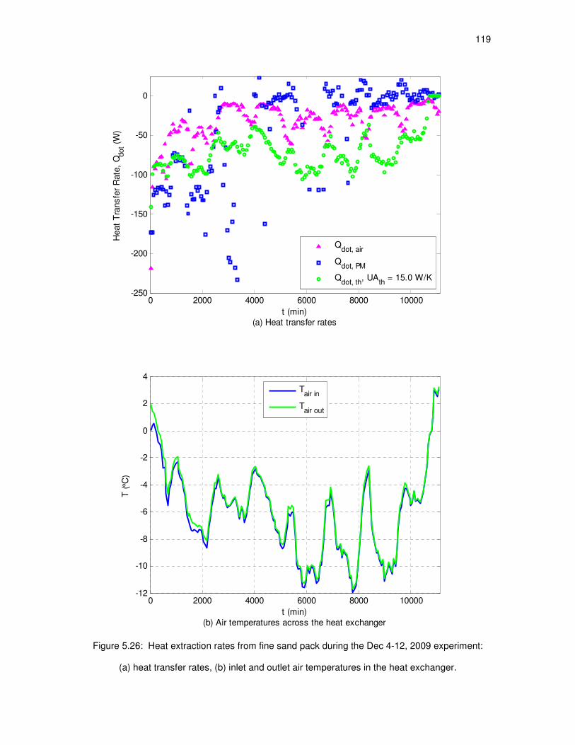
119
Figure 5.26: Heat extraction rates from fine sand pack during the Dec 4-12, 2009 experiment:
(a) heat transfer rates, (b) inlet and outlet air temperatures in the heat exchanger.
0 2000 4000 6000 8000 10000-12
-10
-8
-6
-4
-2
0
2
4
t (min)
(b) Air temperatures across the heat exchanger
T (
°C)
Tair in
Tair out
0 2000 4000 6000 8000 10000-250
-200
-150
-100
-50
0
t (min)
(a) Heat transfer rates
Heat
Tra
nsfe
r R
ate
, Q
dot (
W)
Qdot, air
Qdot, PM
Qdot, th
, UAth
= 15.0 W/K

120
Figure 5.27: Heat extraction rates from fine sand pack during the Dec 26, 2009 – Jan 2, 2010
experiment: (a) heat transfer rates, (b) inlet and outlet air temperatures in the heat exchanger.
0 1000 2000 3000 4000 5000 6000 7000 8000 9000 10000-10
-8
-6
-4
-2
0
2
4
6
t (min)
(b) Air temperatures across the heat exchanger
T (
°C)
Tair in
Tair out
0 1000 2000 3000 4000 5000 6000 7000 8000 9000 10000-250
-200
-150
-100
-50
0
t (min)
(a) Heat transfer rates
Heat
Tra
nsfe
r R
ate
, Q
dot (
W)
Qdot, air
Qdot, PM
Qdot, th
, UAth
= 15.0 W/K
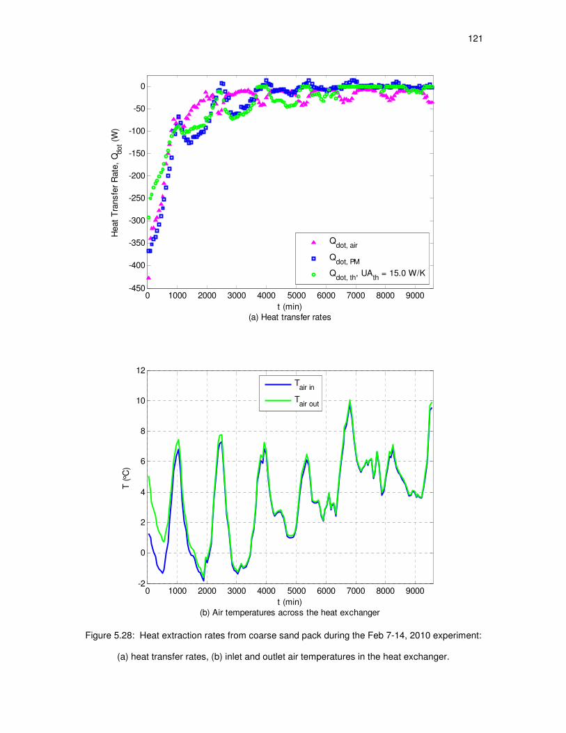
121
Figure 5.28: Heat extraction rates from coarse sand pack during the Feb 7-14, 2010 experiment:
(a) heat transfer rates, (b) inlet and outlet air temperatures in the heat exchanger.
0 1000 2000 3000 4000 5000 6000 7000 8000 9000-2
0
2
4
6
8
10
12
t (min)
(b) Air temperatures across the heat exchanger
T (
°C)
Tair in
Tair out
0 1000 2000 3000 4000 5000 6000 7000 8000 9000-450
-400
-350
-300
-250
-200
-150
-100
-50
0
t (min)
(a) Heat transfer rates
Heat
Tra
nsfe
r R
ate
, Q
dot (
W)
Qdot, air
Qdot, PM
Qdot, th
, UAth
= 15.0 W/K

122
Figure 5.29: Heat extraction rates from coarse sand pack during the Feb 19-25, 2010
experiment: (a) heat transfer rates, (b) inlet and outlet air temperatures in the heat exchanger.
0 1000 2000 3000 4000 5000 6000 7000 8000-6
-4
-2
0
2
4
6
8
t (min)
(b) Air temperatures across the heat exchanger
T (
°C)
Tair in
Tair out
0 1000 2000 3000 4000 5000 6000 7000 8000-350
-300
-250
-200
-150
-100
-50
0
t (min)
(a) Heat transfer rates
Heat
Tra
nsfe
r R
ate
, Q
dot (
W)
Qdot, air
Qdot, PM
Qdot, th
, UAth
= 15.0 W/K

123
Figure 5.30: Heat injection rates into fine sand pack during the Jan 2-4, 2010 experiment: (a)
heat transfer rates, (b) inlet and outlet air temperatures in the heat exchanger.
0 500 1000 1500 2000 2500 300018
18.5
19
19.5
20
20.5
21
21.5
22
t (min)
(b) Air temperatures across the heat exchanger
T (
°C)
Tair in
Tair out
0 500 1000 1500 2000 2500 30000
50
100
150
200
250
300
350
400
450
500
t (min)
(a) Heat transfer rates
Heat
Tra
nsfe
r R
ate
, Q
dot (
W)
Qdot, air
Qdot, PM
Qdot, th
, UAth
= 15.0 W/K

124
Figure 5.31: Heat injection rates into coarse sand pack during the Feb 25-27, 2010 experiment:
(a) heat transfer rates, (b) inlet and outlet air temperatures in the heat exchanger.
0 500 1000 1500 2000 2500 300020.5
21
21.5
22
22.5
23
23.5
24
24.5
25
t (min)
(b) Air temperatures across the heat exchanger
T (
°C)
Tair in
Tair out
0 500 1000 1500 2000 2500 3000-50
0
50
100
150
200
250
300
t (min)
(a) Heat transfer rates
Heat
Tra
nsfe
r R
ate
, Q
dot (
W)
Qdot, air
Qdot, PM
Qdot, th
, UAth
= 15.0 W/K

125
Figure 5.32: Cumulative heat extracted from fine sand pack during the Dec 4-12, 2009
experiment.
0 2000 4000 6000 8000 10000-6
-5
-4
-3
-2
-1
0x 10
7
t (min)
Q (
J)
Qto cool to 0°C
+ Qto freeze
= -1.41e+007 + -4.08e+007 J = -5.49e+007 J
Qcumul, PM
Qcumul, air
Qcumul, air
+ Qcumul, insulation
Qcumul, th
, UAth
= 15.0 W/K
Qcumul, th
+ Qcumul, insulation

126
Figure 5.33: Cumulative heat extracted from fine sand pack during the Dec 26, 2009 – Jan 2,
2010 experiment.
0 1000 2000 3000 4000 5000 6000 7000 8000 9000 10000-6
-5
-4
-3
-2
-1
0x 10
7
t (min)
Q (
J)
Qto cool to 0°C
+ Qto freeze
= -1.46e+007 + -4.08e+007 J = -5.54e+007 J
Qcumul, PM
Qcumul, air
Qcumul, air
+ Qcumul, insulation
Qcumul, th
, UAth
= 15.0 W/K
Qcumul, th
+ Qcumul, insulation
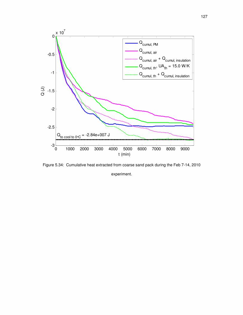
127
Figure 5.34: Cumulative heat extracted from coarse sand pack during the Feb 7-14, 2010
experiment.
0 1000 2000 3000 4000 5000 6000 7000 8000 9000-3
-2.5
-2
-1.5
-1
-0.5
0x 10
7
t (min)
Q (
J)
Qto cool to 0°C
= -2.84e+007 J
Qcumul, PM
Qcumul, air
Qcumul, air
+ Qcumul, insulation
Qcumul, th
, UAth
= 15.0 W/K
Qcumul, th
+ Qcumul, insulation

128
Figure 5.35: Cumulative heat extracted from coarse sand pack during the Feb 19-25, 2010
experiment.
0 1000 2000 3000 4000 5000 6000 7000 8000-2.5
-2
-1.5
-1
-0.5
0x 10
7
t (min)
Q (
J)
Qto cool to 0°C
= -1.99e+007 J
Qcumul, PM
Qcumul, air
Qcumul, air
+ Qcumul, insulation
Qcumul, th
, UAth
= 15.0 W/K
Qcumul, th
+ Qcumul, insulation

129
Figure 5.36: Cumulative heat injected into fine sand pack during the Jan 2-4, 2010 experiment.
0 500 1000 1500 2000 2500 30000
0.5
1
1.5
2
2.5
3
3.5
4
4.5
5x 10
7
t (min)
Q (
J)
Qto w arm up to 0°C
+ Qto thaw
= 2.1e+005 + 3.7e+007 J = 3.8e+007 J
Qcumul, PM
Qcumul, air
Qcumul, air
+ Qcumul, insulation
Qcumul, th
, UAth
= 15.0 W/K
Qcumul, th
+ Qcumul, insulation

130
Figure 5.37: Cumulative heat injected into coarse sand pack during the Feb 25-27, 2010
experiment.
0 500 1000 1500 2000 2500 30000
2
4
6
8
10
12
14
16x 10
6
t (min)
Q (
J)
Qcumul, PM
Qcumul, air
Qcumul, air
+ Qcumul, insulation
Qcumul, th
, UAth
= 15.0 W/K
Qcumul, th
+ Qcumul, insulation

131
the elemental volumes of the porous medium (see Chapter 2 for detailed description of the
methodology) during phase change of water. For calculations, change of phase was determined
based on the temperature of the porous medium, with 0°C set as a threshold. For the same
elemental volume, measured temperature values oscillated back and forth about 0°C from one
time step to another, causing erratic subtraction or addition of the heat of fusion to the energy
content of that volume. As a result, heat extraction or injection rate, %&TJ, also shows up as a
strong scatter on heat transfer rate plots during freezing or thawing periods (see heat transfer
plots in Figure 5.26a, Figure 5.27a, Figure 5.29a and Figure 5.30a).
Based on heat transfer rates, calculated for all heat extraction and injection experiments
(listed in Table 5.1) using the two above-described methods, and the experimental temperature
data, performance characteristics of the thermosiphon was assessed. Namely, its overall heat
transfer coefficient, /rs, was estimated to be approximately 15 W/°C (see Chapter 2 for
detailed methodology). Using the value of /rs = 15Á/°, thermosiphon heat transfer rates,
%&rs, for given temperature differences between the ambient air and the thermosiphon wall,
(pM\ − pHH), were calculated with Equation (2.37) and plotted next to the heat transfer rate
plots of the two previous methods (see Figure 5.26a, Figure 5.27a, Figure 5.28a, Figure 5.29a,
Figure 5.30a, Figure 5.31a). Calculation of heat transfer rates through the thermosiphon provided
an alternative way of estimating heat extraction or injection rates in porous medium.
For visualization of the amount of energy being extracted or injected from/in the porous
medium, cumulative energy removed or injected for the given point in time was calculated using
each method and plotted in Figure 5.32, Figure 5.33, Figure 5.34, Figure 5.35, Figure 5.36 and
Figure 5.37. In order to estimate the total heat lost or gained by the porous medium, heat lost or
gained through tank's insulation, %lJlH,MGIlH, using the overall heat transfer coefficient of the
tank, /rpG¨ = 1.59Á/° (see experimental apparatus details in Chapter 4), was also
calculated and added (dotted lines in the above-mentioned figures) to heat being transferred to
air by the heat exchanger, %lJlH,pM\, and to heat flowing through the thermosiphon, %lJlH,rs.

132
As can be seen in Figure 5.32, cumulative heat extraction plot for the porous medium, %lJlH,éê, drops down rapidly in 3000 min to 4000 min interval, which corresponds to freezing
of water, and thus, removal of a large amount of fusion heat from the porous medium. Most likely,
phase change was occurring during a much longer time period than implied by the %lJlH,éê
plot, which is also indicated by smoother plots based on two other methods in the same figure.
Due to the assumption that all water filling the voids of the elemental volume was frozen
instantly as 0°C temperature threshold was reached (measured by the thermocouples), and
increasing volumes of concentric elemental rings (see Figure 2.3) in the radial direction,
calculations required the subtraction of increasing amounts of fusion heat in each time step as the
freezing front progressed outwards from the thermosiphon. In fact, due to limitations of heat
transfer to the thermosiphon wall, the freezing should have occurred more gradually and the
respective fusion energy could not have been extracted in such a short period of time.
Taking into account the initial temperature of the porous medium, the total amount of
energy that had to be removed from the tank in order to achieve complete freezing of water was
calculated as 5.5·107 Joules and is shown in Figure 5.32 as a sum of heat to be removed to cool
the porous medium from its initial temperature to 0°C, Qto cool to 0°C, and heat of fusion, Qto freeze.
Cumulative heat extraction plots for the porous medium, %lJlH,éê, and for the thermosiphon
(with the correction of heat losses), %lJlH,rs+%lJlH,MGIlHprMLG, approximately agree with the
calculated 5.5·107 Joules needed to be extracted for complete freezing. Cumulative heat
transferred to air, even with the addition of heat losses through the insulation, %lJlH,pM\+%lJlH,MGIlHprMLG, seems to be underestimated, which should be caused by the low
accuracy of the temperature measurements at the inlet and outlet of the heat exchanger.
Reductions in cumulative heat in %lJlH,éê plot at approximately 1500 min and 3000
min in Figure 5.33 correlate with warmer ambient air temperatures (see temperature plots in
Figure 5.27b). During daytime, heat extraction rates from the porous medium were lower due to
smaller temperature difference between the ambient air and the porous medium in the tank. This
caused thawing of the frozen area near thermosiphon walls by the inflow of heat from warmer far-

133
field (areas near the tank walls). The method for %lJlH,éê calculation was based on measured
temperatures and as temperatures in some elemental volumes rose above 0°C (see increasing
porous medium temperatures at 1500 min and 3000 min in Figure 5.9), heat of fusion was added
back to the energy content of those rings, causing reduction in the amount of removed cumulative
energy for those time points.
In the coarse sand pack experiment, during which no freezing had taken place, heat
extraction rate plots are in better agreement (Figure 5.28a). However, plots based on porous
medium energy content, %&TJ, and thermosiphon overall heat transfer coefficient, %&rs, follow
ambient temperature variation, when energy transfer rate to air reflects larger temperature
differences between inlet and outlet air, measured during warmer ambient temperatures (see air
temperature plots in Figure 5.28b). Cumulative energy extraction volumes for the same
experiment, shown in Figure 5.34, are also in better agreement compared to other heat extraction
experiments.
Heat extraction rates shown in Figure 5.29a and cumulative energy extraction rates
shown in Figure 5.35, as in the previous coarse sand experiment, are in a relatively good
agreement and exhibit the same trends described in the previous paragraph. Except during
partial freezing of the porous medium at approximately 3500 min and 5000 min, the porous
medium heat transfer rate, %&TJ, shows a strong scatter, due to inaccuracy and low sensitivity of
thermocouple temperature measurements as mentioned before.
Heat Transfer Rates during Heat Injection into Water-Saturated
Porous Media
Figure 5.30 to Figure 5.37 show heat transfer rates and cumulative energy plots of the
two air conditioning experiments during which heat was injected into frozen (in the case of the
fine sand experiment) or cold (coarse sand experiment) porous medium. At the beginning of the
first air conditioning experiment (frozen fine sand), heat injection caused thawing of ice in the
porous medium, showing up as a strong scatter in heat transfer rate plot, %&TJ, in Figure 5.30a.
134
After melting all ice, by approximately 1000 min, all three heat transfer rate plots exhibit a similar
smooth declining trend (see Figure 5.30a).
Cumulative heat injection plot for %lJlH,éê in Figure 5.36 shows a significant
divergence from the plots of the two other methods. This divergence is due to the assumption that
all water in the porous medium was frozen at the beginning of the experiment and heat of fusion,
corresponding to the total volume of the water, was absorbed by the porous medium, which may
not have been the case. Even though at the beginning of the experiment porous medium
temperatures were approximately at 0°C (see Figure 5.20), some of the water in the porous
medium could have been in liquid phase rather than ice. Thus, much less heat of fusion, Qto thaw,
was needed for melting the ice contained in the porous medium.
In the second air conditioning experiment, where the coarse sand pack was not frozen,
the heat transfer rate plots based on all three methods exhibit a similar smooth declining trend
(Figure 5.31a). As there was no phase change in water, and no heat of fusion addition to the
energy content of the porous medium, cumulative heat injection plots in Figure 5.37 are also in
better agreement.
Maximum heat transfer rates achieved during the experiments described in this chapter
were in the range of 250-350 W, yielding approximately 600-850 W/m2 maximum heat flux for the
experimental aluminum thermosiphon with the underground outer circumferential surface area of
Ath = 0.408 m2. High heat flux capabilities of heat pipes make them good candidates for replacing
the existing inefficient ground heat exchangers (see Chapter 1) with thermosiphon arrays.
Thermosiphon Performance
Another assessment of the experimental thermosiphon performance can be based on the
ice build-up during the early water experiments (not described in detail here, as noted at the
beginning of this chapter) showing uniform growth of ice on the submersed surface of the
thermosiphon (see Figure 5.38).
Also, based on the temperatures along the outer surface of the thermosiphon (see Figure
5.39) in later sand pack experiments, it can be seen that there is little variance in surface

135
(a) (b)
Figure 5.38: Uniform ice build-up during heat extraction experiment on Jan 21-30, 2009.
Figure 5.39: Temperatures on outer surface of the thermosiphon during heat removal experiment
from fine sand pack on Dec 4-12, 2009.
0 2000 4000 6000 8000 10000
-6
-4
-2
0
2
4
6
8
10
t (min)
T (
°C)
Twall7
Twall6
Twall5
Twall4
Twall3
Twall2
Uniform ice build-up
Uniform ice build-up

136
temperature in the vertical direction. The maximum difference between the top (Twall 7) and bottom
(Twall 2) thermocouples, placed 1 meter apart, was approximately 2°C. This indicates a relatively
uniform distribution of the working fluid and heat extraction by its evaporation from the internal
surface of the thermosiphon and shows the effective operation of the wicking mesh placed along
the internal walls of the thermosiphon (Figure 4.2b).

137
References
[1] http://en.wikipedia.org/wiki/Thermocouple (Accessed on July 17, 2011). [2] http://www.peaksensors.co.uk/datarequirements.html (Accessed on July 17, 2011). [3] Lemmon, E. W., McLinden, M. O., Friend, D. G., "Thermophysical Properties of Fluid
Systems," in NIST Chemistry WebBook, NIST Standard Reference Database Number 69, Eds. Linstrom, P. J., Mallard, W. G., National Institute of Standards and Technology, Gaithersburg, MD, 20899, http://webbook.nist.gov (Accessed on July 16, 2011).
[4] IAPWS, Revised Release on the IAPS Formulation 1985 for the Viscosity of Ordinary
Water Substance, International Association for the Properties of Water and Steam, Erlangen, Germany, 1997, 15, http://www.iapws.org/relguide/visc.pdf (Accessed on July 16, 2011).
[5] IAPWS, Revised Release on the IAPS Formulation 1985 for the Thermal Conductivity of
Ordinary Water Substance, International Association for the Properties of Water and Steam, London, 1998, 23, http://www.iapws.org/relguide/thcond.pdf (Accessed on July 16, 2011).
[6] Haynes, W. M., 2010-2011, “CRC Handbook of Chemistry and Physics,” 91
st ed., CRC
Press, Boca Raton, pp. 6-12. [7] Feistel, R, Wagner, W., 2006, “A New Equation of State for H2O Ice Ih,” J. Phys. Chem.
Ref. Data, 35(2), pp. 1021-1047. [8] Andersson, O., Inaba, A., 2005, “Thermal Conductivity of Crystalline and Amorphous Ices
and Its Implications on Amorphization and Glassy Water,” Phys. Chem. Chem. Phys., 7, pp. 1441–1449.
[9] Birch, F., Schairer, J. F., Spicer, H. C., 1942, “Handbook of Physical Constants,”
Geological Society of America, Special Papers, 36, p. 12. [10] Barron, T. H. K., Collins, J. F., Smith, T. W., White, G. K., 1982 , “Thermal Expansion,
Gruneisen Functions and Static Lattice Properties of Quartz,” Journal of Physics C: Solid State Physics, 15, pp. 4311-4326.
[11] Birch, F., Clark, H., 1940, “The Thermal Conductivity of Rocks and Its Dependence upon
Temperature and Composition,” American Journal of Science, pp. 529-558. [12] Incropera, F. P., DeWitt, D. P., 1996, ”Fundamentals of Heat and Mass Transfer,” John
Wiley & Sons, New York, 4th ed.
[13] Touloukian, Y. S., et al, 1970, “Thermophysical Properties of Matter,” Vol. 2, “Thermal
Conductivity – Nonmetallic Solids,” Plenum Press, New York, pp. 174-181. [14] http://www.engineeringtoolbox.com/ice-thermal-properties-d_576.html (Accessed on Sep
6, 2010). [15] Coleman, H. W., Steele, W. G., Jr., 1989, “Experimentation and Uncertainty Analysis for
Engineers,” John Wiley & Sons, New York. [16] Chellaiah, S., Viskanta, R., 1989, "Freezing of Water-Saturated Porous Media in the
Presence of Natural Convection: Experiments and Analysis," J. of Heat Transfer, Transactions of the ASME, 111, pp. 425-432.

138
[17] Reda, D. C., 1986, “Natural Convection Experiments in a Stratified Liquid-Saturated
Porous Medium,” Transactions of the ASME, 108, pp. 660-666. [18] Oosthuizen, P. H., 1988, "The Effects of Free Convection on Steady State Freezing in a
Porous Medium-Filled Cavity," ASME Proc. 1988 National Heat Transfer Conference, HTD-96, 2, Houston, July 24-27, pp. 321-327.

6. NUMERICAL SIMULATIONS
For numerical simulations, a commercial software package ANSYS FLUENT ver.6.3 was
chosen for its ability to model heat transfer in porous media and solidification (phase change) and
its prevalent use in the engineering community. The algorithm used in FLUENT is based on the
enthalpy method of the solution of the Stefan problem with the enthalpy function tied to the liquid
fraction in the evaluated cell in the so-called “mushy” zone (partially solidified region), which itself
is based on the temperature of the mixture at a given node [1, 2]. The first simulation was run to
show the general applicability of the FLUENT 6.3 software package to the type of problems
considered in this work, namely, heat transfer in water-saturated porous media with
freezing/thawing processes and potential contribution from natural convection. The second set of
simulations were run to determine the threshold or the range of Rayleigh numbers at which the
enhancement to the heat transfer due to convection starts. Determining the conditions at which
the natural convection contribution becomes significant to the heat transfer mechanism in the
water-saturated porous medium, would define the respective heat transfer calculation methods
and design criteria for the ground-coupled heat exchangers at near water-freezing temperatures.
Software Limitations and Simplifications
Some of the simplifications and limitations inherent in the use of ANSYS FLUENT to
simulate the anticipated modes of heat transfer are as follows:
• Porous media in FLUENT instead of physical volumetric restriction defined by its
porosity, , is modeled by adding sink terms to the governing momentum equations for
the fluid phase [3]. When, due to solidification, porosity approaches zero, fluid transport
in the solidified regions is not eliminated; rather, fluid velocities in those areas are
significantly reduced.

140
• Specific heat capacity, cp, for the selected material must be entered as a constant value
and cannot be modified using a user-defined function (UDF) [4].
• With the exception of species diffusivities, properties for the solid (ice) and liquid (water)
materials cannot be specified separately [1].
• The volume-averaged thermal conductivity is specified by the following model [3]:
6NN(ë¹ìíîF) = 6N + (1 − )6I (6.1)
The thermal conductivity model (Equation (6.1)) used in FLUENT is the same as the
parallel conductivity model (Equation (3.10)) reviewed in Chapter 3 and yields the maximum
conductivity value for porous media (upper bound by 6Tp\pHHH in Figure 3.15). Even though this
model is often used [5, 6], it is not very accurate and significantly overestimates the effective
conductivity for the porous medium. This is illustrated in Figure 6.1.
For comparison, at about 20°C the experimentally determined values of effective
conductivity were 6TJ,NMG= 2.09 W/m·K and 6TJ,Lp\I = 2.05 W/m·K for fine and coarse
sand packs, and at the same temperature the power model (Equation (3.13)) estimates 6NN(JMG Jpq)= 2.13 W/m·K, when the FLUENT model yields approximately 6NN(ë¹ìíîF)=
4.15 W/m·K. This is an overestimation of thermal conductivity of the porous medium of almost two
times. For this reason and due to relatively small variation of thermal conductivity of the selected
water-saturated porous medium (see Chapter 8 for details) in the temperature range of numerical
simulations (0°C to 20°C), thermal conductivities of sand and water were set constant at 6N= 0.43
W/m·K and 6I= 3.1 W/m·K, so that their volume average for the porosity of = 0.38 in the
FLUENT model would yield approximately 6TJë¹ìíîF= 2.09 W/m·K, matching the
experimentally measured value.

141
Figure 6.1: Application of the thermal conductivity model used in ANSYS FLUENT for water-
saturated sand pack.
275 280 285 290 295 300 305 310 315 3200
1
2
3
4
5
6
7
T (K)
Eff
ective T
herm
al C
onductivity,
λeff
(W
/m⋅K
)
λf
λs
λeff (min+max)
λeff (FLUENT)
λexp f ine ave→ ← λexp coarse ave

142
Domain and Setup for Simulations
The domain for numerical simulations was defined according to geometry and
dimensions of the experimental apparatus. GAMBIT was used to create an axi-symmetric
cylindrical face with the following dimensions (Figure 6.2):
Bottom: (D - d) = 0.61 - 0.11 = 0.25 m
where: D = 0.61 m is the internal diameter of the tank
d = 0.11 m is the thermosiphon diameter.
Height: H = 1.14 m (height of the sand pack inside the tank)
The domain face was meshed with equal side elements of ∆r = ∆z = 0.5 cm near the
thermosiphon wall (adjacent 5 cm) and ∆r = ∆z = 1.0 cm away from it. The total volume of the axi-
symmetric cylinder excluding the thermosiphon was 0.322 m3.
One of the heat removal experiments with a fine grain water-saturated sand pack, run on
December 4-12, 2009, which includes ambient air temperature variation (transient temperature
boundary condition), and freezing (phase change), was chosen for simulations in FLUENT. As
transient boundary condition in FLUENT can be easily defined with a polynomial function, in order
to simulate the experimental temperature conditions on the thermosiphon wall, a 4th degree
polynomial was fitted to the first 2000 min of experimental data (Figure 6.3). The polynomial
function was then incorporated into a User-Defined Function (UDF) for FLUENT (see Appendix F)
and was used as a transient temperature boundary condition for the first 2000 min of simulations.
As most heat losses in the experiments occurred from the top cover of the tank, a convective
boundary condition with heat transfer coefficient of 0.57 W/m2·K (UAtank / Atank = 1.59 W/K / 2.77
m2) was applied to the top surface of the domain. The bottom and vertical surfaces of the tank
were defined as adiabatic.
Most of the properties for fluid (water) and solid (quartz) were specified as temperature-
dependent polynomial functions (see Chapter 3). Exceptions were density of sand, defined as
constant at ρs=2654 kg/m3, and constant values (see previous section) were used for thermal
conductivities of both water and sand.

143
Figure 6.2: Face of axi-symmetric cylindrical domain.
D - d = 0.25 m d = 0.11 m
H =
1.1
4 m
∆r = ∆z = 0.5 cm
∆r = ∆z = 1.0 cm
z
r
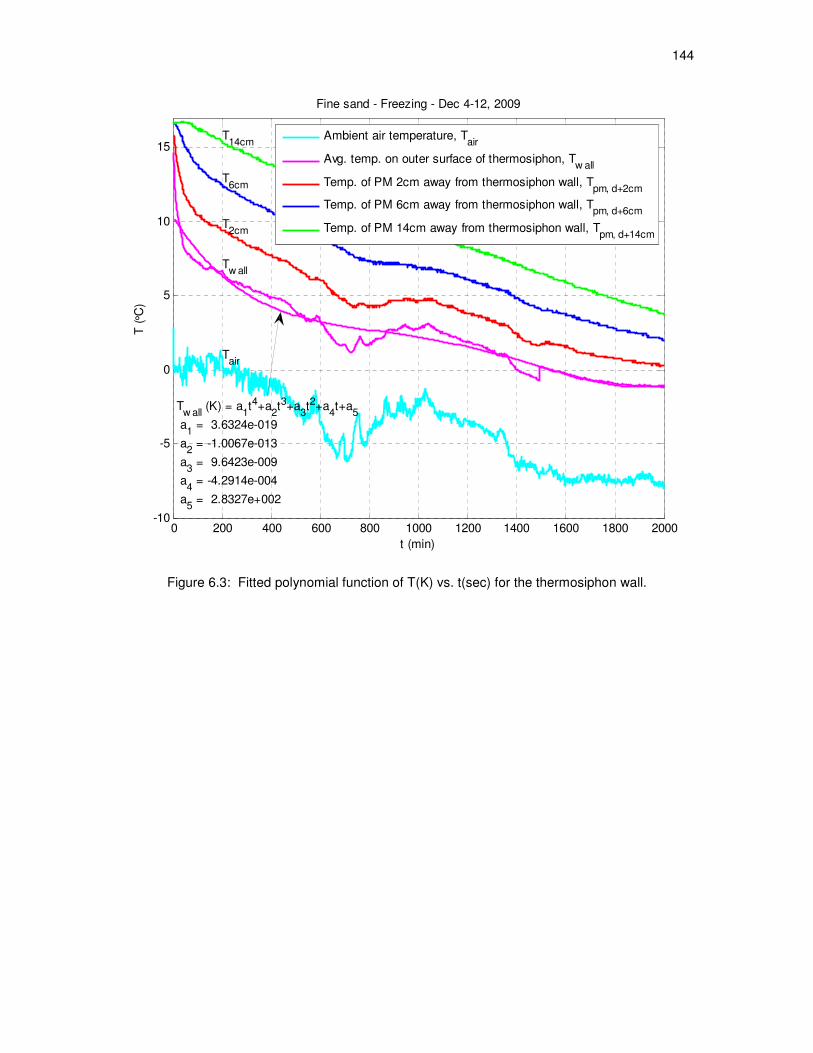
144
Figure 6.3: Fitted polynomial function of T(K) vs. t(sec) for the thermosiphon wall.
0 200 400 600 800 1000 1200 1400 1600 1800 2000-10
-5
0
5
10
15
t (min)
T (
°C)
Fine sand - Freezing - Dec 4-12, 2009
Tair
Tw all
T2cm
T6cm
T14cm
Ambient air temperature, Tair
Avg. temp. on outer surface of thermosiphon, Tw all
Temp. of PM 2cm away from thermosiphon wall, Tpm, d+2cm
Temp. of PM 6cm away from thermosiphon wall, Tpm, d+6cm
Temp. of PM 14cm away from thermosiphon wall, Tpm, d+14cm
Tw all
(K) = a1t4+a
2t3+a
3t2+a
4t+a
5
a1 = 3.6324e-019
a2 = -1.0067e-013
a3 = 9.6423e-009
a4 = -4.2914e-004
a5 = 2.8327e+002

145
Results of Simulation of the Heat Extraction Experiment with a
Transient Temperature Boundary Condition
Results of simulations in ANSYS FLUENT for the first 2000 min of heat extraction from
the water-saturated fine sand experiment conducted on Dec 4-12, 2009 are provided below
(Figure 6.4b, Figure 6.5, Figure 6.6) and compared with the experimental data (Figure 6.4a). A
snapshot of isotherms after 30 h (1800 min) from the beginning of the experiment (Figure 6.4)
shows that experimental and simulated values are in reasonable agreement. Freezing front
location in Figure 6.5b also coincides with the expected location of 0°C isotherm in Figure 6.4a.
As can be seen from the streamlines in Figure 6.5b and fluid velocity vectors in Figure 6.6b,
FLUENT shows natural convection in the simulated porous medium. But, as velocity magnitudes
are negligible, on the order of 10-8
-10-9
m/sec (see Figure 6.6a), very weak convection showing
up in FLUENT simulations should not have any significant effect on the heat transfer in the
porous medium. The conditions at which convective mechanism becomes a significant contributor
to the heat transfer in the porous medium will be shown in the next set of simulations in the
following section.
It can be noticed in Figure 6.6b that the direction of velocity vectors is opposite to what
might be expected due to natural convection adjacent to a thermosiphon wall, which has a lower
temperature than the rest of the fluid/matrix. The reversed direction of flow shown in FLUENT
simulations is due to density maxima of water near 4°C and the transient condition where the
maximum tank temperature was less than 4°C at 30 h (1800 min). Thus, as water was cooled by
the thermosiphon wall below 4°C, its density decreased causing upward movement of the fluid
near the thermosiphon wall due to buoyancy forces.
An interesting illustration of the effect of the water density maxima at 4°C can be seen in
an earlier time snapshot of velocity vectors and corresponding isotherms in Figure 6.7. At this
time, two counterdirectional convective cells were formed (Figure 6.7a), with the highest density
water sinking downwards at approximately the middle of the tank where temperature happens to
be 4°C (see 277 K isotherm in Figure 6.7b).

146
(a) (b)
Figure 6.4: Isotherms after 30 h (1800 min): (a) experimental data and (b) simulations for the
same conditions and geometry.1
1 The text in FLUENT output image was rotated to comply with publishing requirements.
0 0.1 0.2 0.30
0.2
0.4
0.6
0.8
1
- 1-1
0 1 2 3
4
5
Fine Sand - Freezing2009/12/6 03:19:29t = 30.0 h, Ra = -0.3
Tair in
= -7.5°C, Tair out
= -7.1°C
r (m)
z (m
)
2.7
2e
+0
2
2.7
2e
+0
2
2.7
3e
+0
2
2.7
3e
+0
2
2.7
4e
+0
2
2.7
4e
+0
2
2.7
5e
+0
2
2.7
5e
+0
2
2.7
6e
+0
2
Conto
urs
of S
tatic T
em
pera
ture
(K
) (T
ime=
1.0
800e+
05)
Apr
27, 2011
FLU
EN
T 6
.3 (
axi, p
bns, la
m,
unste
ady)

147
(a) (b)
Figure 6.5: Simulation results: (a) freezing front and (b) stream functions after 30 h (1800 min).2
2 The text in FLUENT output images was rotated to comply with publishing requirements.
Freezing front
Apr
27, 2011
FLU
EN
T 6
.3 (
axi, p
bns, la
m,
unste
ady)
Apr
27, 2011
FLU
EN
T 6
.3 (
axi, p
bns, la
m,
unste
ady)
Conto
urs
of S
tream
Function (
Kg/s
) (T
ime=
1.0
800e+
05)
Conto
urs
of Liq
uid
Fra
ction (
Tim
e=
1.0
800e+
05)
0.0
0e
+0
0
4.6
4e
-08
9.2
9e
-08
1.3
9e
-07
1.8
6e
-07
2.3
2e
-07
2.7
9e
-07
3.2
5e
-07
3.7
2e
-07
0.0
0e
+0
0
1.2
5e
-01
2.5
0e
-01
3.7
5e
-01
5.0
0e
-01
6.2
5e
-01
7.5
0e
-01
8.7
5e
-01
1.0
0e
+0
0
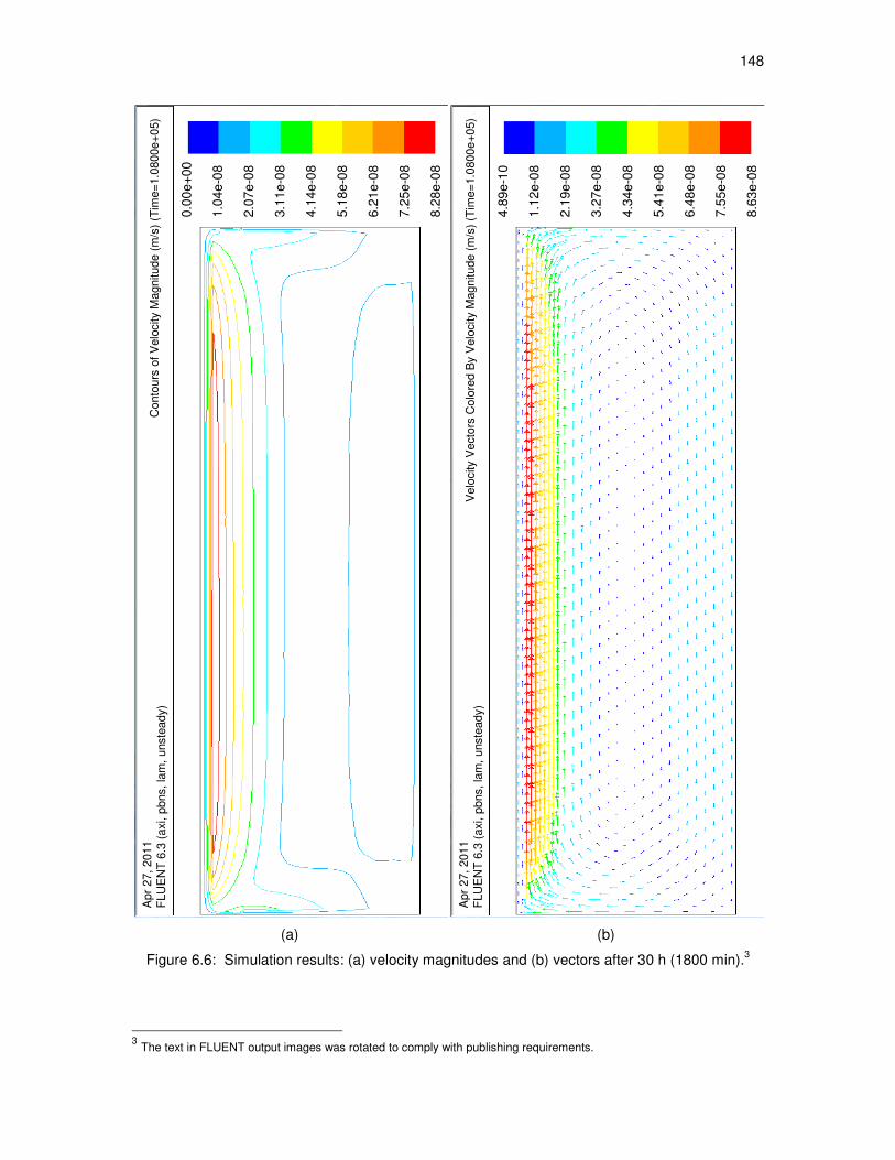
148
(a) (b)
Figure 6.6: Simulation results: (a) velocity magnitudes and (b) vectors after 30 h (1800 min).3
3 The text in FLUENT output images was rotated to comply with publishing requirements.
Apr
27, 2011
FLU
EN
T 6
.3 (
axi, p
bns, la
m,
unste
ady)
Apr
27, 2011
FLU
EN
T 6
.3 (
axi, p
bns, la
m,
unste
ady)
Velo
city
Vecto
rs C
olo
red B
y V
elo
city M
agnitude (
m/s
) (T
ime=
1.0
800e+
05)
Conto
urs
of V
elo
city M
agnitude (
m/s
) (T
ime=
1.0
800e+
05)
4.8
9e
-10
1.1
2e
-08
2.1
9e
-08
3.2
7e
-08
4.3
4e
-08
5.4
1e
-08
6.4
8e
-08
7.5
5e
-08
8.6
3e
-08
0.0
0e
+0
0
1.0
4e
-08
2.0
7e
-08
3.1
1e
-08
4.1
4e
-08
5.1
8e
-08
6.2
1e
-08
7.2
5e
-08
8.2
8e
-08

149
(a) (b)
Figure 6.7: Simulation results: (a) velocity vectors and (b) isotherms after 20 h.4
4 The text in FLUENT output images was rotated to comply with publishing requirements.
Apr
27, 2011
FLU
EN
T 6
.3 (
axi, p
bns, la
m,
unste
ady)
Apr
27, 2011
FLU
EN
T 6
.3 (
axi, p
bns, la
m,
unste
ady)
Velo
city
Vecto
rs C
olo
red B
y V
elo
city M
agnitude (
m/s
) (T
ime=
7.2
000e+
04)
Conto
urs
of S
tatic T
em
pera
ture
(K
) (T
ime=
7.2
000e+
04)
2.7
5e
+0
2
2.7
5e
+0
2
2.7
6e
+0
2
2.7
6e
+0
2
2.7
7e
+0
2
2.7
7e
+0
2
2.7
8e
+0
2
2.7
8e
+0
2
2.7
9e
+0
2
7.4
2e
-12
5.1
2e
-09
1.0
2e
-08
1.5
3e
-08
2.0
4e
-08
2.5
5e
-08
3.0
7e
-08
3.5
8e
-08
4.0
9e
-08

150
The above results of numerical simulations show that FLUENT is capable of simulating
heat transfer in the porous medium with reasonable accuracy and can be used for the heat
transfer studies from/to ground-coupled heat exchangers.
Results of Simulations with Constant Temperature Boundary
Conditions and Different Permeabilities and Initial
Temperatures
For the second set of simulations, the same domain but different boundary and initial
conditions were used. In these simulations, constant temperature boundary condition of Twall= 0°C
or 10°C was applied to the thermosiphon wall and simulations were run for three different
permeabilities, each with two different (uniform) initial temperatures of the porous medium. As in
this case, a section from a long underground thermosiphon cell with impermeable top and bottom
layers of soil (clay layers, for example) was assumed, and adiabatic boundary conditions were
applied to the top, bottom and outer (right wall) boundaries of the domain (Figure 6.2). The initial
driving temperature difference (k − pHH) for the Rayleigh number was set as 20°C by
selecting a 20°C higher than the thermosiphon wall temperature of the porous medium for all
runs. The permeabilities in simulations differed by an order of magnitude, starting with the
measured permeabilities of fine and coarse grain sands (1.93·10-10
m2 and 2.03·10
-9 m
2,
respectively) and the highest permeability used was k=2·10-8
m2. The results of these simulations
are summarized in Figure 6.8, Figure 6.9, Figure 6.10 and Figure 6.11.
As expected, convective transport is the strongest in the warmer, higher permeability
porous medium with maximum water velocities reaching 5·10-4
m/s for k=2·10-8
m2 permeability
and negligible (on the order of 10-6
m/s) in colder, k=1.93·10-10
m2 permeability fine sand pack
(see Figure 6.8). Also, it can be noticed that due to higher viscosity at lower temperatures, fluid
movement subsides faster in colder porous media (see maximum velocity plots of simulations
with lower initial and thermosiphon wall temperatures, Tinit=20°C and Twall=0°C, in Figure 6.8).
Plots of Rayleigh numbers, corresponding to the above-shown maximum velocity plots,
are given in Figure 6.9 with the maximum Ramax=1264 for the warmer, highest permeability
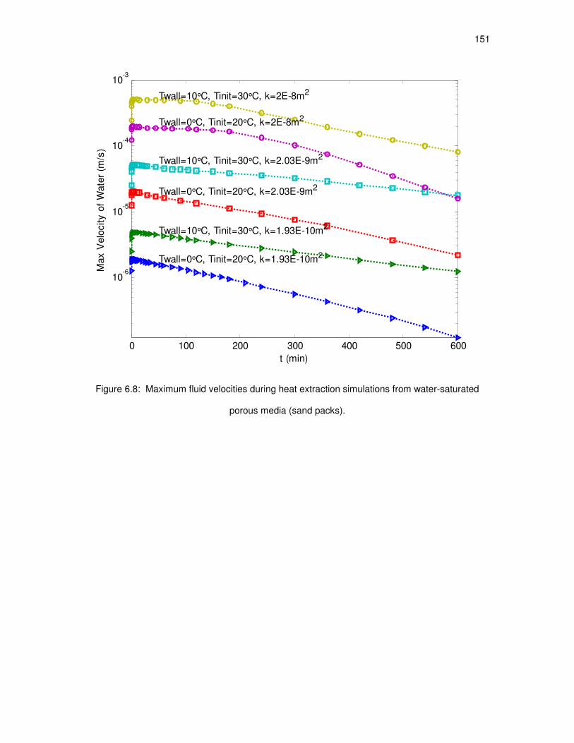
151
Figure 6.8: Maximum fluid velocities during heat extraction simulations from water-saturated
porous media (sand packs).
0 100 200 300 400 500 600
10-6
10-5
10-4
10-3
t (min)
Max V
elo
city o
f W
ate
r (m
/s)
Twall=0°C, Tinit=20°C, k=1.93E-10m2
Twall=10°C, Tinit=30°C, k=1.93E-10m2
Twall=0°C, Tinit=20°C, k=2.03E-9m2
Twall=10°C, Tinit=30°C, k=2.03E-9m2
Twall=0°C, Tinit=20°C, k=2E-8m2
Twall=10°C, Tinit=30°C, k=2E-8m2

152
Figure 6.9: Rayleigh numbers during heat extraction simulations from water-saturated porous
media (sand packs).
0 100 200 300 400 500 60010
0
101
102
103
104
t (min)
Ra
Twall=0°C, Tinit=20°C, k=1.93E-10m2
Twall=10°C, Tinit=30°C, k=1.93E-10m2
Twall=0°C, Tinit=20°C, k=2.03E-9m2
Twall=10°C, Tinit=30°C, k=2.03E-9m2
Twall=0°C, Tinit=20°C, k=2E-8m2
Twall=10°C, Tinit=30°C, k=2E-8m2

153
Figure 6.10: Dependence of maximum fluid velocities on Rayleigh number.
100
101
102
103
104
10-6
10-5
10-4
10-3
uz max
= Ra ⋅ αpm avg
/ L →
Ra
Ma
xim
um
ve
locity o
f w
ate
r (m
/s)
uz max
= Ra ⋅ αpm avg / L
Twall=0°C, Tinit=20°C, k=1.93E-10m2
Twall=10°C, Tinit=30°C, k=1.93E-10m2
Twall=0°C, Tinit=20°C, k=2.03E-9m2
Twall=10°C, Tinit=30°C, k=2.03E-9m2
Twall=0°C, Tinit=20°C, k=2E-8m2
Twall=10°C, Tinit=30°C, k=2E-8m2
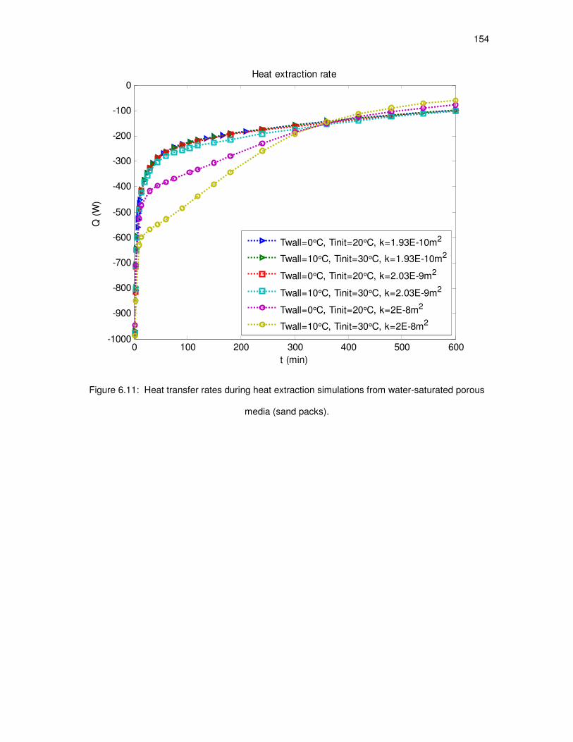
154
Figure 6.11: Heat transfer rates during heat extraction simulations from water-saturated porous
media (sand packs).
0 100 200 300 400 500 600-1000
-900
-800
-700
-600
-500
-400
-300
-200
-100
0
t (min)
Q (
W)
Heat extraction rate
Twall=0°C, Tinit=20°C, k=1.93E-10m2
Twall=10°C, Tinit=30°C, k=1.93E-10m2
Twall=0°C, Tinit=20°C, k=2.03E-9m2
Twall=10°C, Tinit=30°C, k=2.03E-9m2
Twall=0°C, Tinit=20°C, k=2E-8m2
Twall=10°C, Tinit=30°C, k=2E-8m2
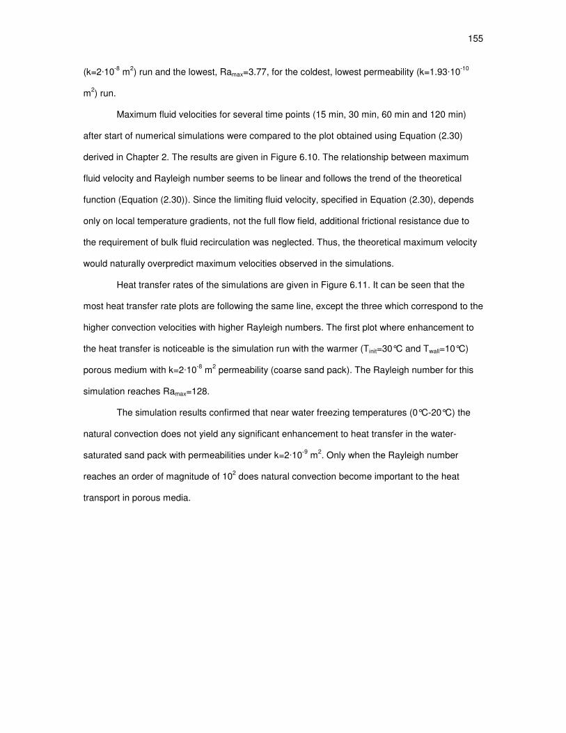
155
(k=2·10-8
m2) run and the lowest, Ramax=3.77, for the coldest, lowest permeability (k=1.93·10
-10
m2) run.
Maximum fluid velocities for several time points (15 min, 30 min, 60 min and 120 min)
after start of numerical simulations were compared to the plot obtained using Equation (2.30)
derived in Chapter 2. The results are given in Figure 6.10. The relationship between maximum
fluid velocity and Rayleigh number seems to be linear and follows the trend of the theoretical
function (Equation (2.30)). Since the limiting fluid velocity, specified in Equation (2.30), depends
only on local temperature gradients, not the full flow field, additional frictional resistance due to
the requirement of bulk fluid recirculation was neglected. Thus, the theoretical maximum velocity
would naturally overpredict maximum velocities observed in the simulations.
Heat transfer rates of the simulations are given in Figure 6.11. It can be seen that the
most heat transfer rate plots are following the same line, except the three which correspond to the
higher convection velocities with higher Rayleigh numbers. The first plot where enhancement to
the heat transfer is noticeable is the simulation run with the warmer (Tinit=30°C and Twall=10°C)
porous medium with k=2·10-8
m2 permeability (coarse sand pack). The Rayleigh number for this
simulation reaches Ramax=128.
The simulation results confirmed that near water freezing temperatures (0°C-20°C) the
natural convection does not yield any significant enhancement to heat transfer in the water-
saturated sand pack with permeabilities under k=2·10-9
m2. Only when the Rayleigh number
reaches an order of magnitude of 102 does natural convection become important to the heat
transport in porous media.

156
References
[1] ANSYS FLUENT ver. 6.3 User's Guide, Chapter 24. [2] Voller, V. R., Prakash, C., 1987, "A Fixed Grid Numerical Modeling Methodology for
Convection-Diffusion Mushy Region Phase-Change Problems," Int. J. Heat Mass Transfer, 30(8), pp. 1709-1719.
[3] ANSYS FLUENT ver. 6.3 User's Guide, Chapter 7.19. [4] ANSYS FLUENT ver. 6.3 UDF Manual, Chapter 1.3 - Limitations. [5] Ogawa, Y., Yamagishi, Y., Kurita, K., 2003, "Evaluation of Melting Process of the
Permafrost on Mars: Its Implication for Surface Features," J. of Geophysical Research, 108(E4), p. 8046.
[6] Wang, B. X., Du, J. H., Peng, X. F., 1998, "Internal Natural, Forced and Mixed
Convection in Fluid-Saturated Porous Medium,” in Transport Phenomena in Porous Media, Edited by Ingham, D. B., Pop, I., Pergamon Press, Oxford, pp. 357-382.

7. GRID-INDEPENDENT AIR CONDITIONING USING
UNDERGROUND THERMAL ENERGY STORAGE
(UTES) AND REVERSIBLE THERMOSIPHON
TECHNOLOGY – EXPERIMENTAL RESULTS
Kekelia, B., Udell, K., 2011, "Grid-Independent Air Conditioning Using Underground Thermal Energy Storage (UTES) and Reversible Thermosiphon Technology - Experimental Results," Proceedings of ASME 5th International Conference on Energy Sustainability and 9th Fuel Cell Science, Engineering and Technology Conference, Washington, D.C.
Reprinted with permission from the American Society of Mechanical Engineers (ASME)

158
Abstract Introduction
Nomenclature
Proceedings of ASME 2011 5th International Conference on Energy Sustainability & 9th Fuel Cell Science, Engineering and Technology Conference
ESFueiCell2011 August 7-10,2011, Washington, DC, USA
ESFue1Ce1l2011-54452
GRID-INDEPENDENT AIR CONDITIONING USING UNDERGROUND THERMAL ENERGY STORAGE (UTES) AND REVERSIBLE THERMOSIPHON TECHNOLOGY -
EXPERIMENTAL RESULTS
ABSTRACT
Bidzina Kekelia University of Utah
Salt Lake City, UT, USA
Thermal energy storage in subsurface soils can produce both inexpensive capacity and storage timescales of the order of a year. In concept, storing excess ambient or solar heat in summer for future winter use and winter "cold" for summer air conditioning can provide essentially zero-carbon space heating and cooling. An innovative ground coupling using a reversible (pump-assisted) thermosiphon with its high heat flux characteristics, intrinsic to two-phase heat pipes, as an inground heat exchanger is proposed and its performance is evaluated in a series of lab-scale experiments. Extraction and injection of heat from/into the watersaturated sand with a single thermosiphon unit representing a cell in an array of thermosiphons is modeled. These results demonstrate that near freezing point of water, due to weak or no natural convection , heat transfer is mainly due to conduction. Also, due to low energy input requirement for pumping working fluid and high heat transfer potential of the reversible thermosiphon, seasonal thermal energy or "cold" storage can be provided for low energy air conditioning applications.
INTRODUCTION Large amount of our energy consumption is used for
heating (space & water) and air conditioning. According to some estimates, building energy demand accounts for almost 40% of the United States' primary energy consumption [1 , 2] and is responsible for about 39% of total US CO2 emissions [1]. Out of this, space & water heating, air conditioning & refrigeration account for approximately 44-48% of the total US building energy
Kent S. Udell University of Utah
Salt Lake City, UT, USA
consumption [1] . Another important indicator is that commercial and residential buildings use approximately 70% of the electricity in the United States [2] large portion of which , again , used for heating & air conditioning. Thus, thermal energy management in buildings constitutes a significant share in our total energy use.
NOMENCLATURE 9 Gravitational acceleration , [m/s2] h Enthalpy [J/kg] H Head [m] k Permeability [m2] L Vertical dimension of the thermosiphon [m] Q Heat [J] Q Heat transfer rate [W]
Ra Rayleigh number LiT Temperature difference [DC or K] vi! Work rate [W]
Greek symbols a Thermal diffusivity [m2/s] f3 Coefficient of thermal expansion [K-'] ." Pump effciency v Kinematic viscosity [m2/s]
Subscripts e Electric
f 9 Liquid to vapor phase change pm Porous media w Water
Copyright © 2011 by ASME

159
Underground Thermal Energy Storage Ground Source Heat Pumps and Ground Coupling Methods
Reversible Thermosiphon Figure 7.1: Passive soil precooling (heat extraction).
UNDERGROUND THERMAL ENERGY STORAGE The idea of thermal energy storage in soil is not new.
The first patent on the use of the ground as a heat sink was issued in Switzerland in 1912 to Swiss engineer and inventor Heinrich Zoelly [3] , better known for his 1903 patent on impulse steam turbine. If soil is used as energy storage medium , it can provide not only a buffer for short term fluctuations in supply and demand, but can accommodate a complete annual heating/cooling load and serve a seasonal balancing function [4-13]. In most cases, if the storage size is restricted on the surface, it can be easily sized to a maximum expected load by a simple increase of depth. The only potential constraint is keeping near-surface ground temperatures close to their natural values to avoid unwanted impact on surface flora and fauna. In climates where winter temperatures drop below O°C, the effective heat capacity can be substantially increased by freezing/melting of water within the soil.
GROUND SOURCE HEAT PUMPS AND GROUND COUPLING METHODS
Ground source heat pumps (GSHP) are the most commonly used technology for utilization of soil for building heating and cooling [3 ,14-20]. An estimated 1.1 million systems have been installed worldwide [17] . GSHPs use vapor compression cycle refrigeration equipment, intermediary heat exchangers and additional circulation pumps for pumping intermediate working fluid (water glycol solution) in underground plastic piping, i.e. , adding equipment and operational costs to the system. Besides, as significant energy (electricity) input is required for the GSHP system to operate, its coefficient of performance (COP) rarely exceeds COPHP < 4 [20] .
The major problem associated with using the ground as a storage medium is in finding an efficient method of extracting or injecting heat. Generally, this is achieved through PVC or polyethylene pipe loops installed horizontally or in vertical U-shaped loops in the boreholes, serving as heat exchangers with soil. In vertical boreholes there is an effect of thermal penalty due to proximity of counter flow of hot and cold working fluid streams in the U-Ioop and exchanging heat with each other [21] . This, of course, increases total borehole length required for the given thermal load of the system.
REVERSIBLE THERMOSIPHON In contrast to GSHPs, a system which is based on an
innovative new concept of using reversible or pumpassisted thermosiphons (Fig. 1 & 2) as the means of ground coupling [12,13], can achieve a very high, if not infinite (in case of passive operation) , coefficient of performance as there is very little or no energy input needed for pumping heat ("cold") from/to soil. Due to
latent heat capture/release phenomena, characteristic of heat pipes and thermosiphons, even a small temperature gradient between the storage medium and heated (cooled) air is a sufficient driving mechanism for moving heat from (to) soil.
In the passive mode of operation a thermosiphon extracts heat from soil and dissipates it with a heat exchanger exposed to cooler ambient air (Fig. 1). In this mode soil temperature has to be higher than that of air.
Oout -cr
Oout ¢::l ~===:.;c::)Oout
Soil Soi l
Figure 1. Passive soil pre-cooling (heat extraction)
In the air cooling (conditioning) mode of operation , the thermosiphon injects heat into the soil (Fig. 2) . This is possible if the thermosiphon is supplemented with a small liquid pump, which supplies colder working liquid from the bottom of thermosiphon to a heat exchanger in the room where air cooling is desired. The liquid evaporates in the heat exchanger taking away heat from the air. Due to pressure gradients, vapors travel back to the colder bottom part of thermosiphon and condense, releasing heat into the soil. Obviously, in this case soil temperatures should be lower than that of the cooled air.
2 Copyright © 2011 by ASME

160
Grid-Independent Air Conditioning System Lab-Scale Prototype
Figure 7.2: Air conditioning mode (heat injection). Figure 7.3: (a) Lab-scale reversible thermosiphon prototype with attached thermocouple array, data logger and heat exchanger, (b) thermosiphon inserted into a thermally insulated tank with
water-saturated sand pack.
Experimental Results and Discussion
Figure 2. Air conditioning mode (heat injection)
GRID-INDEPENDENT AIR CONDITIONING SYSTEM Electrical power required to operate an air
conditioning system based on reversible thermosiphons and underground thermal energy storage is relatively small. Of course, heat exchangers may be fitted with fans or they could be designed to operate passively with the assistance of natural convection . In the latter case, the only power input needed would be for pumping working fluid from the bottom of the thermosiphons to the evaporators in the building . Average power (W) required for this work is
(1)
where Q is the rate of heat removal by the evaporator from the cooled space (the cooling load), htg is the refrigerant enthalpy of vaporization , I1H is the head to be overcome by pumping, rJ is the pump effciency and 9 is the gravitational constant. For a 1 ton (3.517 kW) cooling system, R-134a properties at O°C (htg=198.6 kJ/kg) , rJ = 30% pump efficiency and thermosiphon depth of 50 m, 29 W power would be required for pumping , neglecting losses in the liquid piping. This is not surprising , as due to
large amount of energy associated with the phase change, the amount of refrigerant (R-134a) needed for removal of 3.517 kW of heat is only about 18 g/sec or 14 ml/sec. Thus, all the power needed to operate an airconditioning system with passive heat exchangers could be easily provided by a small solar PV panel coupled with an electric battery.
LA~SCALEPROTOTYPE An experimental prototype of reversible thermosiphon
was designed and built at the Mechanical Engineering Department of the University of Utah. It was made of 11 .5 cm (4.5 in.) diameter, 140 cm (55 in.) long aluminum tube with a forced air heat exchanger on the top (Fig 3a, b) .
(a) (b)
Figure 3. (a) Lab-scale reversible thermosiphon prototype with attached thermocouple array, data logger and heat exchanger, (b) Thermosiphon inserted into a
thermally insulated tank with water saturated sand pack.
An array with 36 thermocouples (Figure 3a) was attached to the side of the thermosiphon wall. Their exact locations are shown by dark gray dots on the isotherm plots (Figs. 7-18) . The thermocouples were connected to a 40 channel data logger [22], which also recorded air temperatures at the inlet and outlet of the heat exchanger.
EXPERIMENTAL RESULTS AND DISCUSSION In order to compare heat transfer in porous media of
different permeabilities, the experiments were conducted with two different average grain size sand packs
3 Copyright © 2011 by ASME

161
Figure 7.4: Heat extraction rate from fine sand. Figure 7.5: Heat extraction rate from coarse sand.
Figure 7.6: Heat injection rate in coarse sand.
saturated (Sw= 1) with water. The sand was sieved in two batches, first one containing particles in the range of 0.50-1.19 mm, and the second batch containing particles in the size of 1.20-4.76 mm. Permeability of each batch was experimentally measured to be kfine=1.93·1Q-l0 m2
(195 Darcy) and kcoarse=2.03·1Q-9 m2 (2059 Darcy) respectively.
The experimental thermosiphon operation was tested in both passive (heat removal) and active (heat injection) modes. Thermally insulated tank was first filled with water saturated fine sand and heat was extracted using ambient winter air (Fig. 3b). After freezing the water, the tank with thermosiphon was rolled into the lab and its operation was reversed starting air conditioning cycle. Several freezing and thawing runs with fine sand were conducted. Then the tank was filled with larger grain size sand and the above experiments were repeated. Sample heat extraction and injection rates of a single thermosiphon system represented by the lab-scale prototype are shown in Fig. 4-6.
§'
Fine sand - Coolin9 -Oct 22-26, 2009 Heat Transfer Rates
50,------,-------,------,-------,------,
-50
~ -100 0"
'" ro IT:
Q)
<f)
ffi .= 1B I
-150
-200
o Data - - - Trend
-400 L--,=-=-=-=T::rre=n=d=co=r=re=c1=edcf=o==r h=e==at=lo=s;:se=s/=9==ai=ns=t=hro==uc9=h t=a=nk=w=a==:oJ1l
o 10 20 30 40 50 t (hour)
Figure 4. Heat extraction rate from fine sand.
Coarse sand -Cooling - Feb 19-25,2010 Heat Transfer Rates
50~----~------~------~------~----~
~ -50 d' .i &l -100 Q)
<f) c ro .=
I I I I - - - - - -1- - - - - - -1- - - - - - -1- - - - - -1- - - 0 - --
1B -150 - I I I 0 - - - -1- - - - - - -I - - - - - - -I - - - - - -
I
-200
-250 L----'=~~~=T=re=nd=c=o=rre=c1=e=d =fo=r =he=at=l=os=se=s=/g==ai=ns=t=hr=ou2'g=h t=a=nk=w=a="J1l
~ 15
0" a)
~ Q)
~ ~ f-
1B I
o 10 20 30 40 50 t (hour)
Figure 5. Heat extraction rate from coarse sand.
250
200
150
100
50
0 0
Coarse sand -Air conditioning - Feb 14-17, 2010 Heat Transfer Rates
o Data - - - Trend --- Trend corrected for heat losses/gains through tank wall
- - - - -1- - - - - - -1- - - - - - -1- - - - - - ---j - - - - - -
I I I - - - - - -1- - - - - - -1- - - - - - -1- - - - --
10 20 30 40 t (hour)
Figure 6. Heat injection rate in coarse sand.
50
The insulated tank was calibrated and its overall heat transfer coefficient (UA) was measured to be approximately 1.59 wrc. Taking into account heat losses/gains to/from the ambient air through the tank insulation, the amount of heat extraction/injection rate from the air passing through the heat exchanger is adjusted by the respective amount and shown by upper/lower red line in Figs. 4-6. The calculated heat transfer rates were based on the change of energy content of porous media in the tank. The volume occupied by the sand pack was divided into 36 concentric
4 Copyright © 2011 by ASME
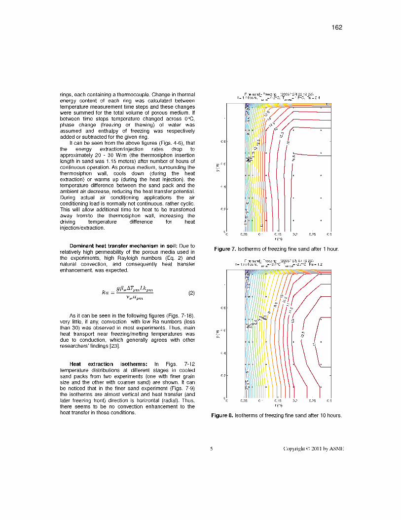
162
Figure 7.7: Isotherms of freezing fine sand after 1 h. Figure 7.8: Isotherms of freezing fine sand after 10 h.
rings, each containing a thermocouple. Change in thermal energy content of each ring was calculated between temperature measurement time steps and these changes were summed for the total volume of porous medium. If between time steps temperature changed across O°C, phase change (freezing or thawing) of water was assumed and enthalpy of freezing was respectively added or subtracted for the given ring.
It can be seen from the above figures (Figs. 4-6), that the energy extraction/injection rates drop to approximately 20 - 30 W/m (the thermosiphon insertion length in sand was 1.15 meters) after number of hours of continuous operation. As porous medium, surrounding the thermosiphon wall, cools down (during the heat extraction) or warms up (during the heat injection), the temperature difference between the sand pack and the ambient air decrease, reducing the heat transfer potential. During actual air conditioning applications the air conditioning load is normally not continuous, rather cyclic. This will allow additional time for heat to be transferred away from/to the thermosiphon wall, increasing the driving temperature difference for heat injection/extraction.
Dominant heat transfer mechanism in soil: Due to relatively high permeability of the porous media used in the experiments, high Rayleigh numbers (Eq. 2) and natural convection, and consequently heat transfer enhancement, was expected.
9 f3w l1Tpm Lkpm R a = -----'-----'-- (2)
As it can be seen in the following figures (Figs. 7-18), very little, if any, convection with low Ra numbers (less than 30) was observed in most experiments. Thus, main heat transport near freezing/melting temperatures was due to conduction, which generally agrees with other researchers' findings [23].
Heat extraction isotherms: In Figs. 7-12 temperature distributions at different stages in cooled sand packs from two experiments (one with finer grain size and the other with coarser sand) are shown. It can be noticed that in the finer sand experiment (Figs. 7-9) the isotherms are almost vertical and heat transfer (and later freezing front) direction is horizontal (radial). Thus, there seems to be no convection enhancement to the heat transfer in these conditions.
0.8
I O.6
>-
OA
0.2
Fine sand - Freezing (2009/12/422:19:29) t = 1.0 hours, Tairin= 0.2°C, Tairout= 1.5°C, Ra = 2A
0.05 0.1 0.15 r(m)
0.2 0.25 0.3
Figure 7. Isotherms of freezing fine sand after 1 hour.
Fine sand - Freezing (2009/12/507:19:29) t = 10.0 hours, Tairin= -3AoC, Tair out= -2.7°C, Ra = 1.2
0.8
I O.6
>-
OA
0.2
Figure 8. Isotherms of freezing fine sand after 10 hours.
5 Copyright © 2011 by ASME

163
Figure 7.9: Isotherms of freezing fine sand after 94 h. Figure 7.10: Isotherms of cooling coarse sand after 1 h. Figure 7.11: Isotherms of cooling coarse sand after 10 h.
0.8
Fine sand - Freezing (2009/12/819:19:29) t=94.0hours, Tairin=-10.I°C, Tairout=-9.8°C, Ra=-O.O
I O.6
>-
OA
0.2
ooL----o-.o~5~~~0.~1----0~.1-5----0~.2-----0~.2-5----0~.3
r(m)
Figure 9. Isotherms of freezing fine sand after 94 hours.
In the heat extraction experiment (Figs. 10-12) using coarse sand, weak counterclockwise convection seems to develop after few hours from the beginning of heat removal, which is apparent from the inclined isotherms in Figs. 10 & 11. Later, as water cools, its viscosity increases, and the temperature difference between the ambient air and porous media decreases, convection ceases (Fig. 12).
Coarse sand - cooli~8 f201 0/2/19020:24:47)
t = 2.0 hours, Tair in= 1.3 , airout= 2.8 C, Ra = 59.0
0.8
I O.6
>-
OA
0.2
Figure 10. Isotherms of cooling coarse sand after 1 hour.
6
Coarse sand - Cooling (2010/2/20 04:24:47) t=10.0hours, Tairin=-0.9°C, Tairout=O.I°C, Ra=31.1
Figure 11. Isotherms of cooling coarse sand after 10 hours.
Copyright © 2011 by ASME

164
Figure 7.12: Isotherms of cooling coarse sand after 40 h. Figure 7.13: Isotherms of heat injection in fine sand after 1 h. Figure 7.14: Isotherms of heat injection in fine sand after 10 h.
Coarse sand - Cooling (2010/2/21 10:24:47) t = 40.0 hours, Tair in= 0.2°C, Tairout= 0.5°C, Ra = 0.9
0.8
I O.6 (j) '(5'
>-
0.4
0.2
ooL----o~.0~5~--0~.1--~-0.~15--~~0.2-----0~.2-5----u0.3
r(m)
Figure 12. Isotherms of cooling coarse sand after 40 hours.
Heat injection isotherms: In Figures 13-18 temperature distribution at different stages of two air conditioning experiments (with fine and coarse sand) are shown. Due to refrigerant leak, the thermosiphon required re-charge before conducting these experiments. Unfortunately, it was over-charged with excessive amount of refrigerant, which filled lower half of the thermosiphon. As a result, only upper part of internal surface of the thermosiphon was available for refrigerant vapor condensation. Thus, higher heat flux can be observed in the upper portion of the thermosiphon wall.
As heat is injected into the porous media and melting front moves away from the thermosiphon (Figs. 13 & 14), the water in the tank warms up and its viscosity drops. After about 15-20 hours weak clockwise natural convection develops (Fig. 15).
Fine sand - Air conditionin~ (2010/1/217:01 :28) t = 1.0 hours, Tairin= 21.3°C, airout= 18.9°C, Ra = -0.0
0.8
I O.6
>-
0.4
0.2
,()."
0 0 0.2 0.25 0.3
Figure 13. Isotherms of heat injection in fine sand after 1 hour.
7
Fine sand - Air conditioning (2010/1/302:01 :28) t = 10.0 hours, Tair in= 21.5°C, Tairout= 20.3°C, Ra = 1.2
0.25 0.3
Figure 14. Isotherms of heat injection in fine sand after 10 hours.
Copyright © 2011 by ASME

165
Figure 7.15: Isotherms of heat injection in fine sand after 24 h. Figure 7.16: Isotherms of heat injection in coarse sand after 1 h. Figure 7.17: Isotherms of heat injection in coarse sand after 10 h.
0.8
I O.6
>-
0.4
0.2
Fine sand -Air conditioning (2010/1/316:01 :28) t=24.0hours, Tairin=21.3°C, Tairout=20.6°C, Ra=2.7
Figure 15. Isotherms of heat injection in fine sand after 24 hours.
The natural convection is stronger in coarse sand experiment (Figs. 16-18), both due to higher temperature (lower viscosity) of the water and higher permeability of larger grain size sand.
8
Coarse sand - Air conditionin~ - (2010/2/1416:38:26) t= 1.0 hours, Tairin=23.2°C, airout=21.8°C, Ra=21.0
Figure 16. Isotherms of heat injection in coarse sand after 1 hour.
Coarse sand -Airconditionin~- (2010/2/1501 :38:26) t = 10.0 hours, Tairin= 24.6°C, air out= 23.9°C, Ra = 39.6
Figure 17. Isotherms of heat injection in coarse sand after 10 hours.
Copyright © 2011 by ASME
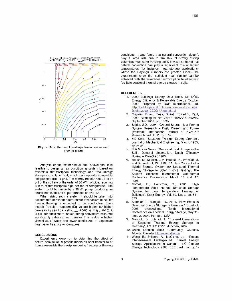
166
Conclusions References
Figure 7.18: Isotherms of heat injection in coarse sand after 24 h.
0.8
I O.6
>-
0.4
0.2
°0~--~~LL~~LO~.li5--~0.-2~--0.~25----0~.3 r(m)
Figure 18. Isotherms of heat injection in coarse sand after 24 hours.
Analysis of the experimental data shows that it is feasible to design an air conditioning system based on reversible thermosiphon technology and free energy ~torage capacity of soil, which can operate completely Independent from a grid. The energy transfer rates into or out of the soil are of the order of 30 W/m of pipe, requiring 120 m of thermosiphon pipe per ton of refrigeration. The system could be driven by a 30 We pump, producing an equivalent coefficient of performance of over 120.
When sizing such a system it should be taken into account that dominant heat transfer mechanism in soil for freezing/thawing is expected to be conduction. Even though Rayleigh numbers (Eq. 2) are higher for higher per~eability s~~d pack (Racoarse=20-60 vs. Rafine=0-1 0), it IS stili not sufficient to induce strong convective cells and s~gnifi~~ntly enhance heat transfer. This is due to higher VISCOSitieS of water and lower coefficients of expansion near water freezing temperatures.
CONCLUSIONS Experiments were run to determine the effect of
natural convection in porous media on heat transfer to or from a reversible thermosiphon during freezing or thawing
conditions. It was found that natural convection doesn't play ~ large role due to the lack of strong driving potentials near water freezing point. It was also found that natural convection can play a significant role at higher temperatures (for instance, heat storage applications) wher~ the Rayleigh numbers are greater. Finally, the experiments show that sufficient heat transfer can be ac~i~ved with the reversible thermosiphon to effectively facilitate seasonal thermal energy storage in soils.
REFERENCES
9
1. 2009 Buildings Energy Data Book, US DOE, Energy Efficiency & Renewable Energy, October 2009, Prepared by D&R International, Ltd. http://bui Idingsdatabook.eren .doe .gov /docs/Data Books/2009 BEDB Updated.pdf
2. Crawley, Drury; Pless, Shanti; Torcellini, Paul; 2009, "Getting to Net Zero," ASHRAE Journal, September 2009, pp. 18-25.
3. Spitler, J.D., 2005, "Ground Source Heat Pumps System Research - Past, Present and Future (Editorial), International Journal of HVAC&R Research. Vol. 11(2):165-167.
4. ME Staff, "Seasonal Thermal Energy Storage", Journal of Mechanical Engineering, March, 1983, pp.28-34.
5. GAM. van Meurs, "Seasonal Heat Storage in the Soil", Doctoral dissertation, Dutch Efficiency Bureau - Pijnacker, 1985.
6. Reuss, M., Mueller, J. P., Roehle, B., Weckler, M. and Schoelkopf, W., 1998, "A New Concept of a Hybrid Storage System for Seasonal Thermal Energy Storage in Solar District Heating", The Second Stockton International Geothermal Conference Proceedings. March 16 and 17, 1998.
7. Nordell, B., Hellstrom, G., 2000, "High Temperature Solar Heated Seasonal Storage System for Low Temperature Heating of Buildings", Solar Energy, Vol. 69, No.6, pp. 511-523.
8. Schmidt, T., ~v1angold, D., 2006, "~~evv Steps in Seasonal Energy Storage in Germany", Ecostock 2006 proceedings, Tenth International Conference on Thermal Energy Storage, May 31-June 2, 2006, Pomona, USA.
9. Mangold, D., Schmidt, T., "The next Generations of Seasonal Thermal Energy Storage in Germany", ESTEC 2007, Munchen, 2007.
10. Drake Landing Solar Community, Okotoks, Alberta, Canada, http://www.dlsc.ca
11. Wong, B.; Snijders, A.; McClung, L.; , "Recent Inter-seasonal Underground Thermal Energy Storage Applications in Canada," EIC Climate Change Technology, 2006 IEEE, vol., no., pp.1-
Copyright © 2011 by ASME

167
7, 10-12 May 2006. SAIC Canada, Ottawa, ON. doi: 10.11 09/EICCCC.2006.277232 URL: http://ieeexplore . ieee .ora/stamp/stamp. jsp?tp=&a rnumber=4057362&isnumber=4057291
12. Udell, K.S., Jankovich, P., Kekelia, B., 2009, "Seasonal Underground Thermal Energy Storage Using Smart Thermosiphon Technology", Geothermal Resources Council 2009 Annual Meeting, GRC Transactions, Reno, NV, Vol. 33, pp.643-647.
13. Udell, K.S., Kekelia, B., Jankovich, P., 2011, "Net Zero Energy Air Conditioning Using Smart Thermosiphon Arrays," 2011 ASH RAE Winter Conference, ASH RAE Transactions, Las Vegas, NV, Vol. 117, Part 1.
14. Ball, D.A., Fischer, R.D., Talbert, S.G., 1983. "State-of-the-Art Survey of Existing Knowledge for the Design of Ground-Source Heat Pumps", Battelle, Columbus, Ohio.
15. Ball, D. A., Fischer, R. D., Hodgett, D.L. 1983. "Design Methods for Ground-Source Heat Pumps", ASHRAE Trans. Vol. 89(2B): 416-440.
16. Svec, O.J. (1987), Potential of ground heat source systems. International Journal of Energy Research, 11: 573-581. doi: 10.1 002/er.444011 0413.
17. Lund, J., et aI., 2004, "Geothermal (groundSource) Heat Pumps - A World Overview", GeoHeat Center Bulletin, September.
18. Sanner, B., 2005, "Examples of GSHP and UTES Systems in Germany", Proceedings World Geothermal Congress 2005, Antalya, Turkey.
10
19. Kirsti Midtt0mme, David Banks, Randi Kalskin Ramstad, Ola M. Scether and Helge Skarphagen, 2008, "Ground-Source Heat Pumps and Underground Thermal Energy Storage - Energy for the future", In Siagstad, T. (ed.) Geology for Society, Geological Survey of Norway. Special Publication, 11, pp. 93-98. http://www.ngu.no/upload/Publikasjoner /Special% 20publication/SP11 08 Midttomme Hl.pdf
20. Straube, John, 2009, "Ground Source Heat Pumps ("Geothermal") for Residential Heating and Cooling: Carbon Emissions and Efficiency," Building Science Digest 113. Accessed on April 15, 2010. http://www.buildingscience.com/docu ments/digest s/bsd-113-ground-source-heat-pumpsgeothermal-for-residential-heating-and-coolingcarbon-emissions-and-efficiency?fu II view= 1
21. Bernier, M.A., "Closed-Loop Ground-Coupled Heat Pump Systems", ASHRAE Journal, September 2006.
22. Data Logger, Graphtec midi LOGGER GL800. Graphtec America, Inc. http://www.graphtecusa.com/
23. Beckermann, C., Viskanta, R., 1988, "Natural Convection Solid/Liquid Phase Change in Porous Media", Int. J. Heat Mass Transfer, Vol. 31, NO.1, pp.35-46.
Copyright © 2011 by ASME

8. ENERGY STORAGE IN DRY SOILS: RAYLEIGH NUMBERS FOR
AIR-SATURATED VS. WATER-SATURATED POROUS MEDIA
Aside from heat transfer in water-saturated soil analyzed in previous chapters, it would be
interesting to determine whether natural convection enhancement takes place when cooling or
heating dry soil (or moist cold soil, where water is immobile and density gradients of soil gas due
to water vapor pressure gradients are negligible).
It has been shown [1, 2], that the enhancement to the heat transfer from a vertical pipe
wall due to natural convection may become noticeable as the Rayleigh number, defined by
Equation (2.24), increases above 10-40. Thus, for similar thermosiphon temperatures and
effective permeabilities, k, of the adjacent soil, would natural convection be more likely in water-
saturated or air-saturated soils? To answer that question, characteristic parameters for the
physical properties of the two fluids, and respectively, for the porous media saturated with water
and air, must be specified.
In Figure 8.1, kinematic viscosities of air and water are shown. As viscosity of air drops
with the temperature, the same property for water increases with the temperature drop. Similar
opposing behavior can be seen in Figure 8.2 for thermal expansion coefficients: increasing for air
and decreasing for water as temperature drops.
For illustration of differences in behavior for various permeabilities, porous media with
two different mean particle diameters (dm=0.5 mm & dm=1.0 mm) were selected. Porosity was
taken at = 40% and temperature difference between heated/cooled surface and far-field was
taken at = (I − k) = 10. Permeability of porous media with known average particle
sizes can be calculated using the Carman-Kozeny equation (Equation (2.40)). Thermal diffusivity
of porous medium can be calculated from Equation (8.1):
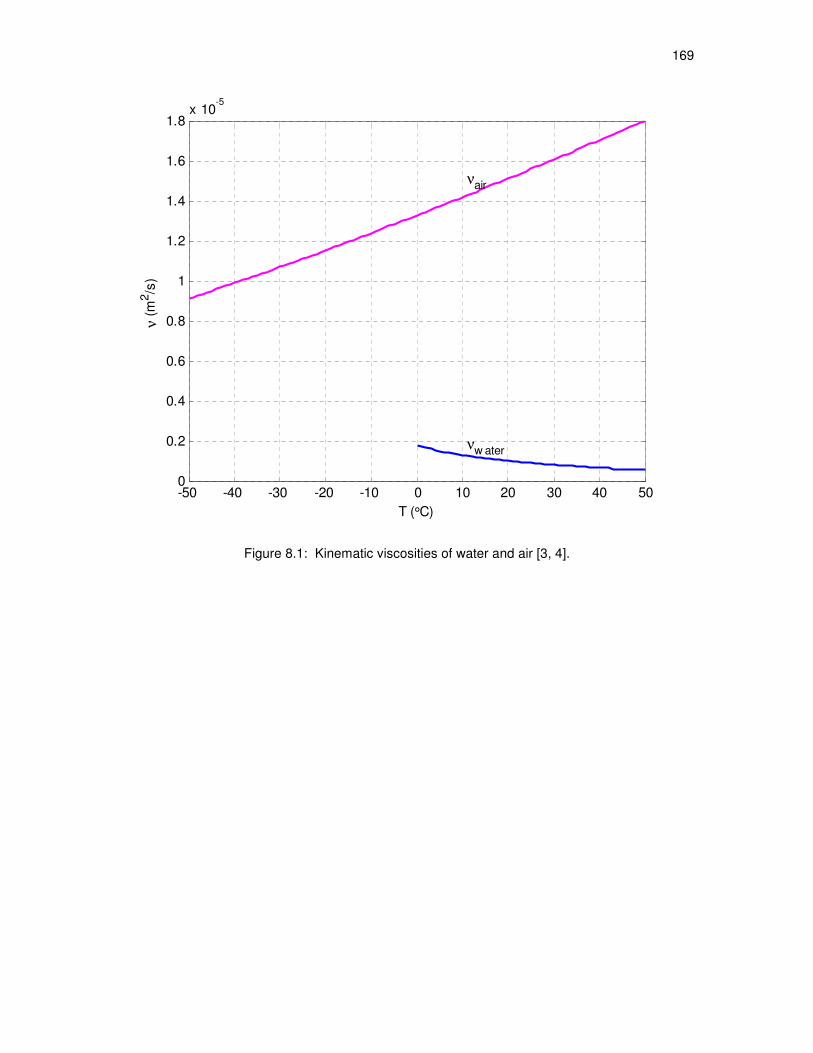
169
Figure 8.1: Kinematic viscosities of water and air [3, 4].
-50 -40 -30 -20 -10 0 10 20 30 40 500
0.2
0.4
0.6
0.8
1
1.2
1.4
1.6
1.8x 10
-5
T (°C)
ν (
m2/s
)
νw ater
νair
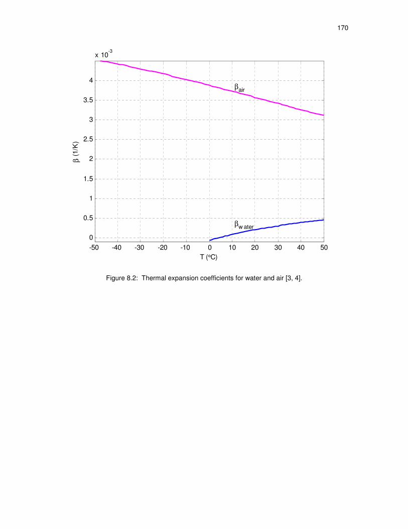
170
Figure 8.2: Thermal expansion coefficients for water and air [3, 4].
-50 -40 -30 -20 -10 0 10 20 30 40 50
0
0.5
1
1.5
2
2.5
3
3.5
4
x 10-3
T (°C)
β (
1/K
)
βw ater
βair
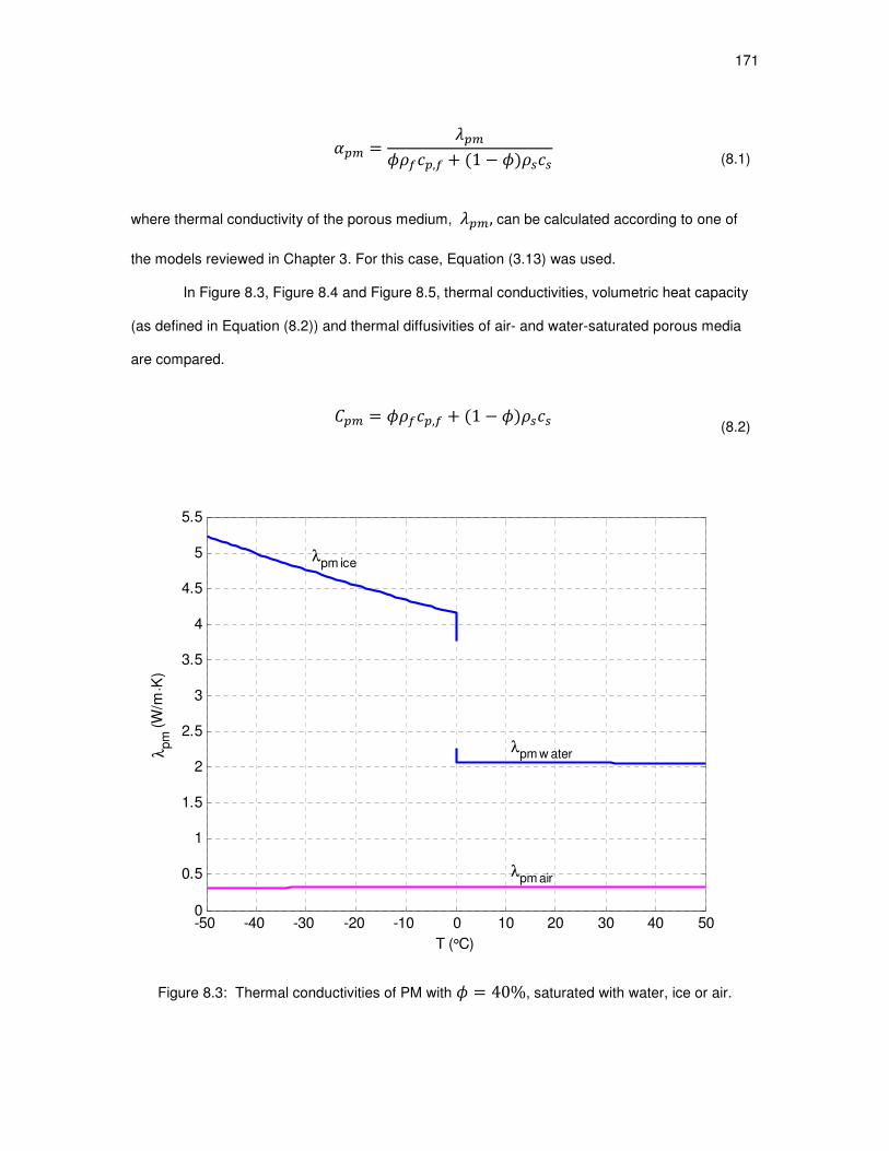
171
2TJ = 6TJ9NT,N + (1 − )9II (8.1)
where thermal conductivity of the porous medium, 6TJ,can be calculated according to one of
the models reviewed in Chapter 3. For this case, Equation (3.13) was used.
In Figure 8.3, Figure 8.4 and Figure 8.5, thermal conductivities, volumetric heat capacity
(as defined in Equation (8.2)) and thermal diffusivities of air- and water-saturated porous media
are compared.
TJ = 9NT,N + (1 − )9II (8.2)
Figure 8.3: Thermal conductivities of PM with = 40%, saturated with water, ice or air.
-50 -40 -30 -20 -10 0 10 20 30 40 500
0.5
1
1.5
2
2.5
3
3.5
4
4.5
5
5.5
T (°C)
λpm
(W
/m⋅K
)
λpm w ater
λpm ice
λpm air
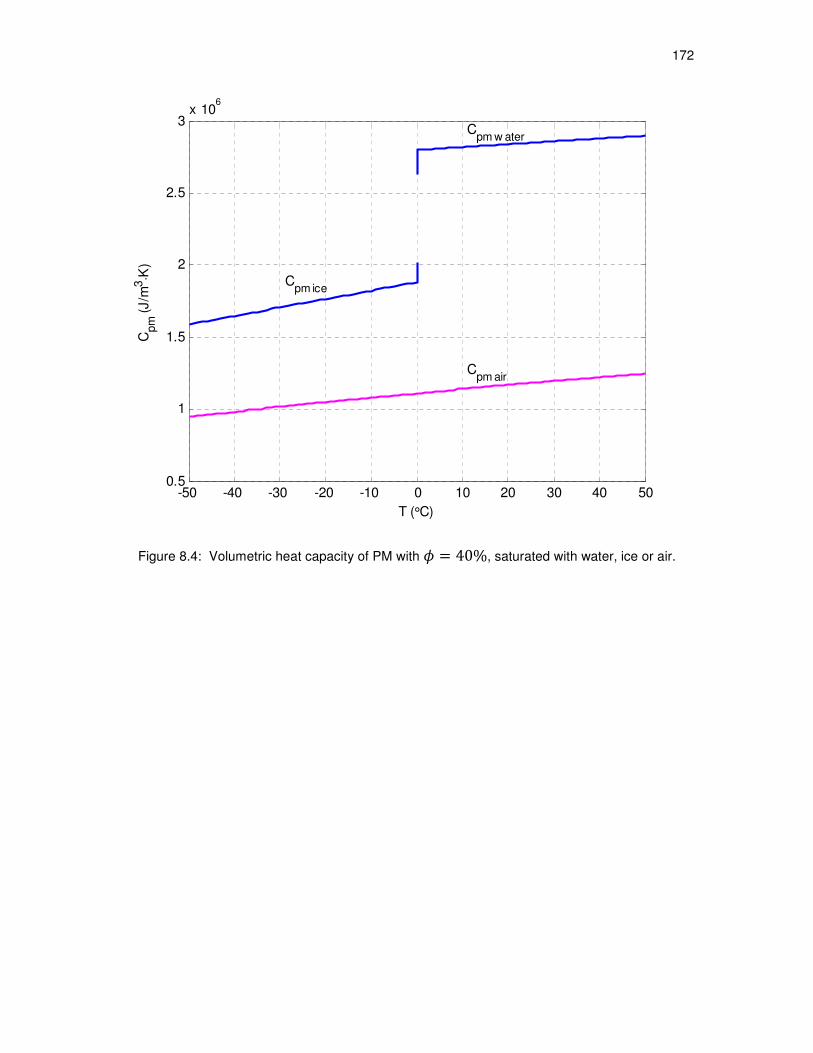
172
Figure 8.4: Volumetric heat capacity of PM with = 40%, saturated with water, ice or air.
-50 -40 -30 -20 -10 0 10 20 30 40 500.5
1
1.5
2
2.5
3x 10
6
T (°C)
Cpm
(J/m
3⋅K
)C
pm w ater
Cpm ice
Cpm air

173
Figure 8.5: Thermal diffusivities of PM with = 40%, saturated with water, ice or air.
-50 -40 -30 -20 -10 0 10 20 30 40 500
0.5
1
1.5
2
2.5
3
3.5x 10
-6
T (°C)
αpm
(m
2/s
)
αpm w ater
αpm ice
αpm air
174
Finally, Rayleigh numbers for air-saturated porous media were calculated and compared
to that of water-saturated porous media. The results are presented in Figure 8.6. It is interesting
to observe that in contrast to diminishing convection (Ra dropping below 10) for water-saturated
porous medium as temperature approaches freezing point (0°C), Rayleigh numbers for air
increase as temperature drops (Figure 8.6), indicating that convective cells could be developing
assisting heat transfer while cooling dry soils. Explanation of this phenomenon lies in the opposite
behavior of viscosities and thermal expansion coefficients of gases versus water (see Figure 8.1
and Figure 8.2). This causes the Rayleigh number (Equation (2.24)) to increase for air- and
decrease for water-saturated porous media as temperature decreases. Thus, when removing
heat from air-saturated porous media and lowering its temperature, onset of natural convection
(Ra is 102 order of magnitude) can be expected, enhancing heat transfer from soils with high gas
content.
It should be also noted that, generally, air-saturated porous media has inferior ability to
transmit heat (due to lower thermal conductivity, see Figure 8.3, and diffusivity, see Figure 8.5) or
store thermal energy (due to lower thermal capacitance, see Figure 8.4), than water-saturated
porous media. Higher water content in soil would always be desirable, especially when
temperatures below 0°C are attained and freezing of water is possible.

175
Figure 8.6: Ra numbers for water- vs. air-saturated porous medium
( = 1.0, = 40%, ∆ = 10°).
-50 -40 -30 -20 -10 0 10 20 30 40 50
0
50
100
150
T (°C)
Ra
pm
Raw
, dm
=0.5mm Ra
a, d
m=0.5mm
Raw
, dm
=1.0mm
Raa, d
m=1.0mm
Raw
, dm
= 0.5mm, kpm
= 2.5e-010m2
Raw
, dm
= 1.0mm, kpm
= 9.9e-010m2
Raa, d
m= 0.5mm, k
pm= 2.5e-010m2
Raa, d
m= 1.0mm, k
pm= 9.9e-010m2

176
References
[1] Beckermann, C., Viskanta, R., 1988, "Natural Convection Solid/Liquid Phase Change in Porous Media," Int. J. Heat and Mass Transfer, 31(1), pp. 35-46.
[2] Chellaiah, S., Viskanta, R., 1989, "Freezing of Water-Saturated Porous Media in the
Presence of Natural Convection: Experiments and Analysis," J. of Heat Transfer, Transactions of the ASME, 111, pp. 425-432.
[3] Air properties data obtained from: http://www.engineeringtoolbox.com/dry-air-properties-
d_973.html (Accessed on Apr 13, 2011). [4] Haynes, W. M., 2010-2011, “CRC Handbook of Chemistry and Physics,” 91
st ed., CRC
Press, Boca Raton, pp. 6-12.

9. DISCUSSION AND CONCLUSIONS
As it was seen from the results obtained in this work, the dominant heat transfer
mechanism to (from) a thermosiphon from (to) adjacent porous media, imitating water-saturated
soil conditions near 0°C, is conduction. Thus, using a conduction model for determining and
simulating heat transfer from/to a thermosiphon in soil for a UTES-based air conditioning system,
is a reasonable assumption. In order to compensate higher water viscosities at lower
temperatures, for Rayleigh numbers to exceed 100 (even though natural convection was
observed in the experiments at Rayleigh numbers of 30 and above, its contribution to heat
transfer is insignificant until Rayleigh number reaches approximately 100), it would require very
long vertical sections (on the order of 100 meters or more) of high permeability soils, without clay
or impermeable rock layers, for development of strong natural convection cells capable of
significantly enhancing the heat transfer. But geology where there are thick regions with high
vertical permeabilities (comparable to those used in this study) would be rare, which would
essentially preclude development of natural convection near thermosiphon walls.
At the same time, as it has been shown in numerical simulations in Chapter 6, at warmer
temperatures (20°C-30°C or higher) of the water-saturated porous medium, Rayleigh numbers of
over 100 may be achieved inducing strong natural convection with high fluid velocities and
enhancing heat transfer to/from the thermosiphon. Thus, if UTES is used for heat storage rather
than development of a “cold sink” for air conditioning applications, then natural convection in the
soil should be taken into account and respective model applied for determining design
parameters of such a heating system.
Numerical simulations also showed that the maximum fluid velocities, .Jpq , due to
natural convection were found near the thermosiphon wall and increased linearly (according to
the following relationship: .Jpq = ( Ü´¹ ) with the Rayleigh number.

178
From the analysis presented in Chapter 8, it can be seen that Rayleigh numbers for air-
saturated porous media near water freezing temperatures increase with decreasing
temperatures. Thus, natural convection may develop during heat transfer in dry or low water
content porous media at lower temperatures, with Ra reaching 100 or more, depending on soil
permeability and driving temperature difference. This is an opposite behavior from what was
observed for the same conditions for water-saturated porous media, where natural convection
ceases as porous media temperature approaches 0°C due to increase in water viscosity and
decrease of its thermal expansion coefficient.
Even though natural convection enhancement may be anticipated during heat transfer in
dry soils, its low volumetric thermal capacity, compared to water-saturated soils, makes it less
desirable for cold storage, unless there is sufficient moisture in the soil to significantly increase its
thermal capacity due to its latent heat of fusion. On the other hand, low thermal conductivity and
diffusivity of air-saturated soil may prove beneficial, due to its resistance to heat dissipation, for
long-term high-temperature thermal energy storage applications.
For the modeling needs of the thermal energy storage system examined in this study,
particularly heat transfer from thermosiphons in soil with freezing and thawing water, ANSYS
FLUENT software package can be used, but would require adjustment of its thermal conductivity
model and boundary condition modifications using user-defined functions (UDFs). Due to its
limitations and simplifications (discussed in Chapter 6), FLUENT may not be the best modeling
means for the given task, but it is still able to provide reasonable results. It is recommended that
along with FLUENT’s application, other models and methods, mentioned in Chapter 2, be
explored and tested for optimal modeling solution.

APPENDIX A
A - MATLAB CODE FOR FITTING POLYNOMIAL FUNCTIONS
TO SAND (QUARTZ) PROPERTIES
%Bidzina Kekelia, 2009-2011 clear, clc %SAND (QUARTZ) PROPERTIES (temperature dependent: T in Celcius) %---------- %SAND (QUARTZ): Thermal Conductivity %---------- %Quartz - Frank Incropera, David DeWitt, Fundamentals of Heat and Mass %Transfer, 4th ed., 1996. %parallel to optical axis: Ts1=[100 200 300 400 600 800]; %K Ts1=Ts1-273; %C lam_s1=[39 16.4 10.4 7.6 5.0 4.2]; %W/(m*K) %perpendicular to opt axis: Ts2=Ts1; %C lam_s2=[20.8 9.5 6.21 4.70 3.4 3.1]; %W/(m*K) %---------- %Qartz (parallel) - Francis Birch & Harry Clark, The thermal
conductivity %of rocks and its dependence upon temperature and composition, American %Journal of Science, p529-558, 1940. %parallel to optical axis: Ts3=[0 50 100 150 200 250 300 350]; %C lam_s3=[27.3 22.4 19.0 16.8 15.1 13.6 12.3 11.3]; %x10^-3
cal/(cm*sec*C) lam_s3=lam_s3*0.41868; %converting to W/(m*K) %perpendicular to optical axis: Ts4=[0 50 100 150 200 250 300 350]; %C lam_s4=[16.3 13.5 11.8 10.6 9.7 8.9 8.4 7.9]; %x10^-3 cal/(cm*sec*C) lam_s4=lam_s4*0.41868; %converting to W/(m*K) %---------- %Curve fitting with polynomial combined data of Incropera & Dewitt,
1996 %and Birch & Clark, 1940: Ts_fitdata=[-73 0 27 50 100 127 150 200 250 300 327 350]; %C lam_fitdata=[9.5 16.3*0.41868 6.21 13.5*0.41868 11.8*0.41868 4.70 ... 10.6*0.41868 9.7*0.41868 8.9*0.41868 8.4*0.41868 3.4 7.9*0.41868];
%W/(m*K) fitlam=polyfit(Ts_fitdata,lam_fitdata,3); lam_fit=polyval(fitlam,Ts_fitdata); R2_fitlam=corrcoef(lam_fitdata,lam_fit); %---------- %Qartz Monzonite - Francis Birch & Harry Clark, 1940

180
Ts5=[0 50 100 150 200]; %C lam_s5=[7.56 6.98 6.55 6.20 5.91]; %x10^-3 cal/(cm*sec*C) lam_s5=lam_s5*0.41868; %converting to W/(m*K) %---------- %Quartzitic Sandstone - Francis Birch & Harry Clark, 1940 %parallel to bed: Ts6=[0 50 100 150 200]; %C lam_s6=[13.6 11.8 10.6 9.7 9.0]; %x10^-3 cal/(cm*sec*C) lam_s6=lam_s6*0.41868; %converting to W/(m*K) %perpendicular to bed: Ts7=[0 50 100 150 200]; %C lam_s7=[13.1 11.4 10.3 9.35 8.65]; %x10^-3 cal/(cm*sec*C) lam_s7=lam_s7*0.41868; %converting to W/(m*K) %---------- %Quartzite - Enson, 1931 Ts8=[0 100]; %C lam_s8=[6.24 5.23]; %W/(m*K) %---------------------------------------------------------------------- figure(1) plot(Ts1,lam_s1,'d','MarkerFaceColor','b','LineWidth',2), hold on plot(Ts2,lam_s2,'md','MarkerFaceColor','m','LineWidth',2) plot(Ts3,lam_s3,'v','LineWidth',2) plot(Ts4,lam_s4,'mv','LineWidth',2) plot(Ts_fitdata,lam_fit,'m--','LineWidth',2) plot(Ts5,lam_s5,'o-.',Ts6,lam_s6,'o-.',Ts7,lam_s7,'o-.',... Ts8,lam_s8,'o-.','LineWidth',2) xlabel('T_s (\circC)') ylabel('Thermal Conductivity, \lambda_solid (W/m\cdotK)') %title('Sand Properties: Thermal Conductivity of Quartz') xlim([-100 400]) ylim([0 18]) legend('Quartz, parallel to opt axis - Incropera & Dewitt, 1996',... 'Quartz, perpendicular to opt axis - Incropera & Dewitt, 1996',... 'Quartz, parallel to opt axis - Birch & Clark, 1940',... 'Quartz, perpendicular to opt axis - Birch & Clark, 1940',... '3^r^d degree polynomial fit of Incropera&DeWitt,1996 and
Birch&Clark,1940',... 'Qartz Monzonite - Francis Birch & Harry Clark, 1940',... 'Quartzitic Sandstone, parallel to bed - Birch & Clark, 1940',... 'Quartzitic Sandstone, perpendicular to bed - Birch & Clark,
1940',... 'Quartzite - Enson, 1931') ax=[0.7 0.64]; ay=[0.4 0.287]; annotation('textarrow',ax,ay,'string',... '\lambda_solid= a_1T^3+a_2T^2+a_3T+a_4',... [' a_1 = ',num2str(fitlam(1),'%10.4e')],... [' a_2 = ',num2str(fitlam(2),'%10.4e')],... [' a_3 = ',num2str(fitlam(3),'%10.4e')],... [' a_4 = ',num2str(fitlam(4),'%10.4e')],... [' R^2 = ',num2str(R2_fitlam(2),'%10.5f')],... 'HorizontalAlignment','Left');%,'FontSize',10); %====================================================================== %SAND (QUARTZ): Specific Heat %---------- %Quartz - Frank Incropera, David DeWitt, Fundamentals of Heat and Mass %Transfer, 4th ed., 1996.

181
TTs1=[300 400 600 800]; %K TTs1=TTs1-273; %C cp_s1=[745 885 1075 1250]; %J/(kg*K) %---------- %Quartz - Francis Birch, J.F. Schairer, H. Cecil Spicer, Handbook of %Physical Constants, Geological Society of America, Special Papers, ... %Number 36, p224, 1942. TTs2=[-200 0 200 400]; %C cp_s2=[173 698 969 1129]; %J/(kg*K) %For 0<T<575 deg C: a=0.7574; b=0.607e-3; c=0.168e5; TTs3=273:10:673; %K for i=1:length(TTs3) cp_s3(i)=(a+b*TTs3(i)-c*TTs3(i)^-2)*1000; %J/(kg*K) end TTs3=TTs3-273; %C %---------- %Quartz - T H K Barron, J F Collins, T W Smith, G K White, Thermal %expansion, Gruneisen functions and static lattice properties of
quartz, %Journal of Physics C: Solid State Physics, volume 15, p4311-4326, 1982 TTs4=[75 85 100 125 150 175 200 225 250 273 283 293 298 373 473 573
673];%K TTs4=TTs4-273; %C cp_s4=[179 212 261 339.9 414 481.8 543.3 599.4 651.2 696.7 714.5 733
... 741 853 965 1059 1123]; %J/(kg*K) %---------- fitcp=polyfit(TTs4,cp_s4,3); cp_s4_fit=polyval(fitcp,TTs4); R2_fitcp=corrcoef(cp_s4,cp_s4_fit); %---------------------------------------------------------------------- figure(2) plot(TTs1,cp_s1,'^','MarkerSize',8,'LineWidth',2), hold on plot(TTs2,cp_s2,'s','MarkerSize',8,'LineWidth',2) plot(TTs3,cp_s3,'-.','LineWidth',2) plot(TTs4,cp_s4,'ro','MarkerSize',5,'LineWidth',2) plot(TTs4,cp_s4_fit,'r--','LineWidth',2) xlabel('T_s (\circC)') ylabel('Heat Capacity, c_p solid (J/kg\cdotK)') %title('Sand Properties: Heat Capacity of Quartz') xlim([-250 450]) ylim([0 1200]) legend('Incropera & Dewitt, 1996',... 'Birch, et al,1942',... 'c_p=a+bT-cT^-^2, only for 0<T<575\circC, Birch, et al,1942',... 'Barron, et al, 1982',... '3^r^d degree polynomial fit of Barron, et al,1982 data',... 'Location','SouthEast') ax=[0.54 0.37]; ay=[0.55 0.535]; annotation('textarrow',ax,ay,'string',... 'c_p solid= a_1T^3+a_2T^2+a_3T+a_4',... [' a_1 = ',num2str(fitcp(1),'%10.4e')],... [' a_2 = ',num2str(fitcp(2),'%10.4e')],...

182
[' a_3 = ',num2str(fitcp(3),'%10.4e')],... [' a_4 = ',num2str(fitcp(4),'%10.4e')],... [' R^2 = ',num2str(R2_fitcp(2),'%10.5f')],... 'HorizontalAlignment','Left');%,'FontSize',10); %====================================================================== %SAND (QUARTZ): Density %---------- %Quartz - http://www.mindat.org/min-3337.html den_s1=2660; %kg/m3 TTTs1=20; %C %Quartz - http://webmineral.com/data/Quartz.shtml den_s2=2620; %kg/m3 TTTs2=20; %C %Quartz - http://rruff.geo.arizona.edu/doclib/hom/quartz.pdf den_s3=2650; %kg/m3 TTTs3=20; %C %Quartz -
http://www.mineralatlas.com/mineral%20general%20descriptions/Q/quartzpc
d.htm den_s4=2655; %kg/m3 TTTs4=20; %C %Quartz - Francis Birch, J.F. Schairer, H. Cecil Spicer, Handbook of %Physical Constants, Geological Society of America, Special Papers, ... %Number 36, p12, 1942. den_s5=2654; %kg/m3 TTTs5=20; %C %Quartz - Frank Incropera, David DeWitt, Fundamentals of Heat and Mass %Transfer, 4th ed., 1996. den_s6=2650; %kg/m3 TTTs6=27; %C %----------------------------------------------------------------------

APPENDIX B
B - MATLAB CODE FOR FITTING POLYNOMIAL FUNCTIONS
TO WATER PROPERTIES
%Bidzina Kekelia, 2009-2011 %---------- %WATER PROPERTIES (temperature dependent: T in Celcius) %Sources: NIST database, Journal Metrologia, Wikipedia %====================================================================== clear, clc %====================================================================== %PROPERTIES based on NIST database data: %====================================================================== %Reading in from NIST data file [T,p,den,v,e,h,s,Cv,Cp,c,JT,miu,k,phase] = ... textread('WaterpropertiesNISTdata.txt',... '%f%f%f%f%f%f%f%f%f%f%f%f%f%s','commentstyle','matlab'); %---------------------------------------------------------------------- %DENSITY - Curve fitting of data from NIST database fit1=polyfit(T,den,4); den_fit=polyval(fit1,T); R2_fit1=corrcoef(den,den_fit); figure(1), plot(T,den,'bo','MarkerSize',2,'LineWidth',2), grid on, hold
on plot(T,den_fit,'b-.','LineWidth',2), hold on xlabel('T (\circC)'), ylabel('\rho (kg/m^3)'); %title('Water Density Variation with Temperature' % '(Curve-fitting NIST data)') ylim([988,1001]) ax=[0.57 0.538]; ay=[0.67 0.657]; annotation('textarrow',ax,ay,'string',... '\rho_water = a_1T^4+a_2T^3+a_3T^2+a_4T+a_5',... [' a_1 = ',num2str(fit1(1),'%10.4e')],... [' a_2 = ',num2str(fit1(2),'%10.4e')],... [' a_3 = ',num2str(fit1(3),'%10.4e')],... [' a_4 = ',num2str(fit1(4),'%10.4e')],... [' a_5 = ',num2str(fit1(5),'%10.4e')],... [' R^2 = ',num2str(R2_fit1(2),'%10.5f')],... 'HorizontalAlignment','Right');%,'FontSize',10); %---------------------------------------------------------------------- %HEAT CAPACITY (Cp) - Curve fitting of data from NIST database fit2=polyfit(T,Cp,4); Cp_fit=polyval(fit2,T); R2_fit2=corrcoef(Cp,Cp_fit);

184
figure(2), plot(T,Cp,'bo','MarkerSize',2,'LineWidth',2), grid on, hold
on plot(T,Cp_fit,'b-.','LineWidth',2) xlabel('T (\circC)'), ylabel('c_p (kJ/kg\cdotK)'); %title('Water Heat Capacity c_p Variation with Temperature' % '(Curve-fitting NIST data)') ylim([4.172,4.22]) legend('NIST data points','4^t^h degree polynomial fit',... 'Location','NorthEast'); ax=[0.4 0.36]; ay=[0.411 0.38]; annotation('textarrow',ax,ay,'string',... 'c_p = a_1T^4+a_2T^3+a_3T^2+a_4T+a_5',... [' a_1 = ',num2str(fit2(1),'%10.4e')],... [' a_2 = ',num2str(fit2(2),'%10.4e')],... [' a_3 = ',num2str(fit2(3),'%10.4e')],... [' a_4 = ',num2str(fit2(4),'%10.4e')],... [' a_5 = ',num2str(fit2(5),'%10.4e')],... [' R^2 = ',num2str(R2_fit2(2),'%10.5f')],... 'HorizontalAlignment','L');%,'FontSize',10); %---------------------------------------------------------------------- %DYNAMIC VISCOSITY (miu) - Curve fitting of data from NIST database fit3=polyfit(T,miu,4); miu_fit=polyval(fit3,T); R2_fit3=corrcoef(miu,miu_fit); figure(3), plot(T,miu,'bo','MarkerSize',2,'LineWidth',2), grid on, hold
on plot(T,miu_fit,'b-.','LineWidth',2), hold on xlabel('T (\circC)'), ylabel('\mu (Pa\cdots)'); %title('Water Dynamic Viscosity Variation with Temperature' % '(Curve-fitting NIST data)') ax=[0.55 0.482]; ay=[0.49 0.42]; annotation('textarrow',ax,ay,'string',... '\mu = a_1T^4+a_2T^3+a_3T^2+a_4T+a_5',... [' a_1 = ',num2str(fit3(1),'%10.4e')],... [' a_2 = ',num2str(fit3(2),'%10.4e')],... [' a_3 = ',num2str(fit3(3),'%10.4e')],... [' a_4 = ',num2str(fit3(4),'%10.4e')],... [' a_5 = ',num2str(fit3(5),'%10.4e')],... [' R^2 = ',num2str(R2_fit3(2),'%10.5f')],... 'HorizontalAlignment','L');%,'FontSize',10); %---------------------------------------------------------------------- %KINEMATIC VISCOSITY (niu) - based on NIST data curvefits (niu = miu /
den) for i=1:length(T) niu(i)=miu(i)/den(i); end figure(4), plot(T,niu,'bo','MarkerSize',2,'LineWidth',2), grid on, hold
on xlabel('T (\circC)'), ylabel('\nu (m^2/s)'); %title('Water Kinematic Viscosity Variation with Temperature' % '(\nu = \mu / \rho)') %---------------------------------------------------------------------- %Thermal Conductivity - Curve fitting of data from NIST database fit4=polyfit(T,k,4); k_fit=polyval(fit4,T);
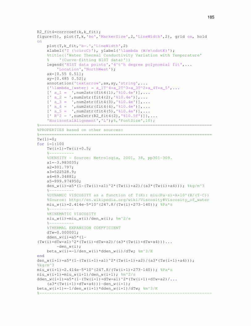
185
R2_fit4=corrcoef(k,k_fit); figure(5), plot(T,k,'bo','MarkerSize',2,'LineWidth',2), grid on, hold
on plot(T,k_fit,'b-.','LineWidth',2) xlabel('T (\circC)'), ylabel('\lambda (W/m\cdotK)'); %title('Water Thermal Conductivity Variation with Temperature' % '(Curve-fitting NIST data)') legend('NIST data points','4^t^h degree polynomial fit',... 'Location','NorthWest'); ax=[0.55 0.51]; ay=[0.485 0.52]; annotation('textarrow',ax,ay,'string',... '\lambda_water = a_1T^4+a_2T^3+a_3T^2+a_4T+a_5',... [' a_1 = ',num2str(fit4(1),'%10.4e')],... [' a_2 = ',num2str(fit4(2),'%10.4e')],... [' a_3 = ',num2str(fit4(3),'%10.4e')],... [' a_4 = ',num2str(fit4(4),'%10.4e')],... [' a_5 = ',num2str(fit4(5),'%10.4e')],... [' R^2 = ',num2str(R2_fit4(2),'%10.5f')],... 'HorizontalAlignment','L');%,'FontSize',10); %====================================================================== %PROPERTIES based on other sources: %====================================================================== Tw(1)=0; for i=1:100 Tw(i+1)=Tw(i)+0.5; %---------- %DENSITY - Source: Metrologia, 2001, 38, pp301-309. a1=-3.983035; a2=301.797; a3=522528.9; a4=69.34881; a5=999.974950; den_w(i)=a5*(1-(Tw(i)+a1)^2*(Tw(i)+a2)/(a3*(Tw(i)+a4))); %kg/m^3 %---------- %DYNAMIC VISCOSITY as a function of T(K): miu(Pa·s)=A×10^(B/(T-C)) %Source: http://en.wikipedia.org/wiki/Viscosity#Viscosity_of_water miu_w(i)=2.414e-5*10^(247.8/(Tw(i)+273-140)); %Pa*s %---------- %KINEMATIC VISCOSITY niu_w(i)=miu_w(i)/den_w(i); %m^2/s %---------- %THERMAL EXPANSION COEFFICIENT dTw=0.000001; dden_w(i)=a5*(1-
(Tw(i)+dTw+a1)^2*(Tw(i)+dTw+a2)/(a3*(Tw(i)+dTw+a4)))... -den_w(i); beta_w(i)=-1/den_w(i)*dden_w(i)/dTw; %m^3/K end den_w(i+1)=a5*(1-(Tw(i+1)+a1)^2*(Tw(i+1)+a2)/(a3*(Tw(i+1)+a4)));
%kg/m^3 miu_w(i+1)=2.414e-5*10^(247.8/(Tw(i+1)+273-140)); %Pa*s niu_w(i+1)=miu_w(i+1)/den_w(i+1); %m^2/s dden_w(i+1)=a5*(1-(Tw(i+1)+dTw+a1)^2*(Tw(i+1)+dTw+a2)/... (a3*(Tw(i+1)+dTw+a4)))-den_w(i+1); beta_w(i+1)=-1/den_w(i+1)*dden_w(i+1)/dTw; %m^3/K %----------------------------------------------------------------------
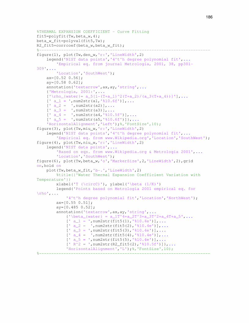
186
%THERMAL EXPANSION COEFFICIENT - Curve Fitting fit5=polyfit(Tw,beta_w,4); beta_w_fit=polyval(fit5,Tw); R2_fit5=corrcoef(beta_w,beta_w_fit); %---------------------------------------------------------------------- figure(1), plot(Tw,den_w,'r:','LineWidth',2) legend('NIST data points','4^t^h degree polynomial fit',... 'Empirical eq. from journal Metrologia, 2001, 38, pp301-
309',... 'Location','SouthWest'); ax=[0.52 0.56]; ay=[0.58 0.62]; annotation('textarrow',ax,ay,'string',... 'Metrologia, 2001:',... ['\rho_water= a_5[1-(T+a_1)^2(T+a_2)/(a_3(T+a_4))]'],... [' a_1 = ',num2str(a1,'%10.6f')],... [' a_2 = ',num2str(a2)],... [' a_3 = ',num2str(a3)],... [' a_4 = ',num2str(a4,'%10.5f')],... [' a_5 = ',num2str(a5,'%10.6f')],... 'HorizontalAlignment','Left');%,'FontSize',10); figure(3), plot(Tw,miu_w,'r:','LineWidth',2) legend('NIST data points','4^t^h degree polynomial fit',... 'Empirical eq. from www.Wikipedia.org','Location','SouthWest'); figure(4), plot(Tw,niu_w,'r:','LineWidth',2) legend('NIST data points',... 'Based on eqs. from www.Wikipedia.org & Metrologia 2001',... 'Location','SouthWest'); figure(6), plot(Tw,beta_w,'o','MarkerSize',2,'LineWidth',2),grid
on,hold on plot(Tw,beta_w_fit,'b-.','LineWidth',2) %title('Water Thermal Expansion Coefficient Variation with
Temperature') xlabel('T (\circC)'), ylabel('\beta (1/K)') legend('Points based on Metrologia 2001 empirical eq. for
\rho',... '4^t^h degree polynomial fit','Location','NorthWest'); ax=[0.55 0.51]; ay=[0.485 0.52]; annotation('textarrow',ax,ay,'string',... '\beta_water = a_1T^4+a_2T^3+a_3T^2+a_4T+a_5',... [' a_1 = ',num2str(fit5(1),'%10.4e')],... [' a_2 = ',num2str(fit5(2),'%10.4e')],... [' a_3 = ',num2str(fit5(3),'%10.4e')],... [' a_4 = ',num2str(fit5(4),'%10.4e')],... [' a_5 = ',num2str(fit5(5),'%10.4e')],... [' R^2 = ',num2str(R2_fit5(2),'%10.5f')],... 'HorizontalAlignment','L');%,'FontSize',10); %----------------------------------------------------------------------

APPENDIX C
C - MATLAB CODE FOR FITTING POLYNOMIAL FUNCTIONS
TO ICE PROPERTIES
%Bidzina Kekelia, 2009-2011 %---------- %ICE PROPERTIES (temperature dependent: T in Celcius) %====================================================================== clear, clc %Reading in from data file obtained from: %2010-2011 CRC Handbook of Chemistry and Physics, 91st ed., p.6-12. [T,den_ice,lam_ice,Cp_ice]=textread('Icedata - CRC Handbook.txt',... '%f%f%f%f','commentstyle','matlab'); %---------------------------------------------------------------------- %DENSITY - Curve fitting of data fit1=polyfit(T,den_ice,3); den_ice_fit=polyval(fit1,T); R2_fit1=corrcoef(den_ice,den_ice_fit); figure(1), plot(T,den_ice,'bo','MarkerSize',2,'LineWidth',2),grid
on,hold on plot(T,den_ice_fit,'b-.','LineWidth',2), hold on xlabel('T (\circC)'), ylabel('\rho_ice (kg/m^3)'); %title('Ice Density Variation with Temperature') xlim([-50,0]) %ylim([0.75,1.35]) legend('CRC Handbook data points',... '3^rd degree polynomial fit (T in \circC)',... 'Location','NE'); ax=[0.46 0.55]; ay=[0.45 0.50]; annotation('textarrow',ax,ay,'string',... ['\rho_ice= a_1T^3+a_2T^2+a_3T+a_4'],... [' a_1 = ',num2str(fit1(1),'%10.4e')],... [' a_2 = ',num2str(fit1(2),'%10.4e')],... [' a_3 = ',num2str(fit1(3),'%10.4e')],... [' a_4 = ',num2str(fit1(4),'%10.4e')],... [' R^2 = ',num2str(R2_fit1(2),'%10.5f')],... 'HorizontalAlignment','Left'); %---------------------------------------------------------------------- %CONDUCTIVITY - Curve fitting of data fit2=polyfit(T,lam_ice,3); lam_ice_fit=polyval(fit2,T); R2_fit2=corrcoef(lam_ice,lam_ice_fit); figure(2), plot(T,lam_ice,'bo','MarkerSize',2,'LineWidth',2),grid
on,hold on plot(T,lam_ice_fit,'b-.','LineWidth',2), hold on

188
xlabel('T (\circC)'), ylabel('\lambda_ice (W/m\cdotK)'); %title('Ice Thermal Conductivity Variation with Temperature') xlim([-50,0]) %ylim([2.2,2.8]) legend('CRC Handbook data data points',... '3^rd degree polynomial fit (T in \circC)',... 'Location','NE'); ax=[0.42 0.54]; ay=[0.46 0.54]; annotation('textarrow',ax,ay,'string',... ['\lambda_ice= a_1T^3+a_2T^2+a_3T+a_4'],... [' a_1 = ',num2str(fit2(1),'%10.4e')],... [' a_2 = ',num2str(fit2(2),'%10.4e')],... [' a_3 = ',num2str(fit2(3),'%10.4e')],... [' a_4 = ',num2str(fit2(4),'%10.4e')],... [' R^2 = ',num2str(R2_fit2(2),'%10.5f')],... 'HorizontalAlignment','Left'); %---------------------------------------------------------------------- %HEAT CAPACITY - Curve fitting of data fit3=polyfit(T,Cp_ice,3); Cp_ice_fit=polyval(fit3,T); R2_fit3=corrcoef(Cp_ice,Cp_ice_fit); figure(3), plot(T,Cp_ice,'bo','MarkerSize',2,'LineWidth',2),grid
on,hold on plot(T,Cp_ice_fit,'b-.','LineWidth',2), hold on xlabel('T (\circC)'), ylabel('C_p ice (J/kg\cdotK)'); %title('Ice Specific Heat Capacity Variation with Temperature') xlim([-50,0]) %ylim([2,3.6]) legend('CRC Handbook data data points',... '3^rd degree polynomial fit (T in \circC)',... 'Location','SE'); ax=[0.61 0.48]; ay=[0.45 0.50]; annotation('textarrow',ax,ay,'string',... ['C_p ice= a_1T^3+a_2T^2+a_3T+a_4'],... [' a_1 = ',num2str(fit3(1),'%10.4e')],... [' a_2 = ',num2str(fit3(2),'%10.4e')],... [' a_3 = ',num2str(fit3(3),'%10.4e')],... [' a_4 = ',num2str(fit3(4),'%10.4e')],... [' R^2 = ',num2str(R2_fit3(2),'%10.5f')],... 'HorizontalAlignment','Left');
%----------------------------------------------------------------------
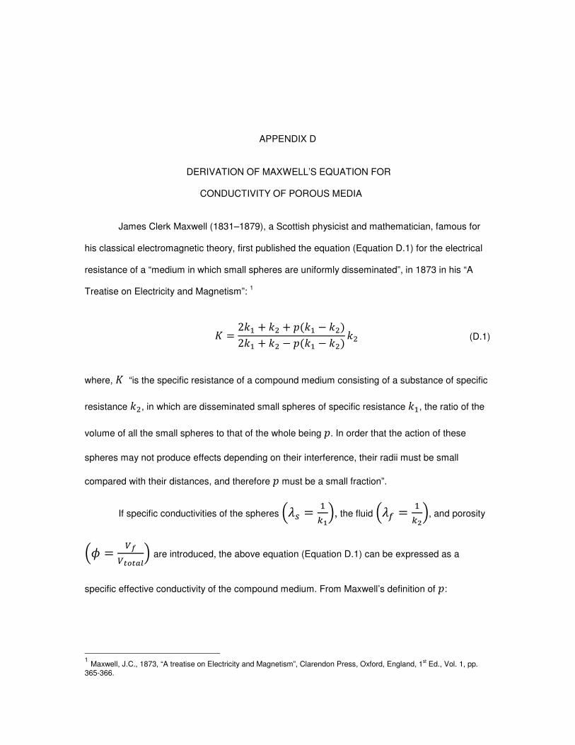
APPENDIX D
D - DERIVATION OF MAXWELL’S EQUATION FOR
CONDUCTIVITY OF POROUS MEDIA
James Clerk Maxwell (1831–1879), a Scottish physicist and mathematician, famous for
his classical electromagnetic theory, first published the equation (Equation D.1) for the electrical
resistance of a “medium in which small spheres are uniformly disseminated”, in 1873 in his “A
Treatise on Electricity and Magnetism”: 1
= 2 + U + B( − U)2 + U − B( − U) U (D.1)
where, “is the specific resistance of a compound medium consisting of a substance of specific
resistance U, in which are disseminated small spheres of specific resistance , the ratio of the
volume of all the small spheres to that of the whole being B. In order that the action of these
spheres may not produce effects depending on their interference, their radii must be small
compared with their distances, and therefore B must be a small fraction”.
If specific conductivities of the spheres µ6I = «·, the fluid µ6N =
¶·, and porosity
µ = ð®ð³Ã³ñ· are introduced, the above equation (Equation D.1) can be expressed as a
specific effective conductivity of the compound medium. From Maxwell’s definition of B:
1 Maxwell, J.C., 1873, “A treatise on Electricity and Magnetism”, Clarendon Press, Oxford, England, 1
st Ed., Vol. 1, pp.
365-366.
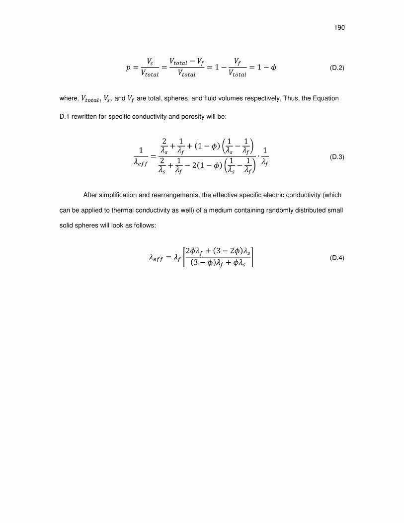
190
B = 0I0rLrpH = 0rLrpH − 0N0rLrpH = 1 − 0N0rLrpH = 1 − (D.2)
where, 0rLrpH, 0I, and 0N are total, spheres, and fluid volumes respectively. Thus, the Equation
D.1 rewritten for specific conductivity and porosity will be:
16NN =26I + 16N + (1 − ) g 16I − 16Nh26I + 16N − 2(1 − ) g 16I − 16Nh ∙
16N (D.3)
After simplification and rearrangements, the effective specific electric conductivity (which
can be applied to thermal conductivity as well) of a medium containing randomly distributed small
solid spheres will look as follows:
6NN = 6N 26N + (3 − 2)6I(3 − )6N + 6I (D.4)
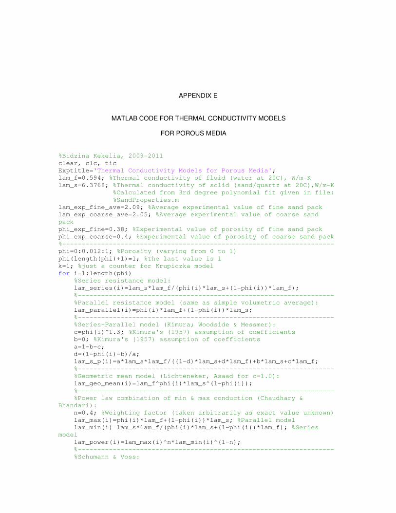
APPENDIX E
E - MATLAB CODE FOR THERMAL CONDUCTIVITY MODELS
FOR POROUS MEDIA
%Bidzina Kekelia, 2009-2011 clear, clc, tic Exptitle='Thermal Conductivity Models for Porous Media'; lam_f=0.594; %Thermal conductivity of fluid (water at 20C), W/m-K lam_s=6.3768; %Thermal conductivity of solid (sand/quartz at 20C),W/m-K %Calculated from 3rd degree polynomial fit given in file: %SandProperties.m lam_exp_fine_ave=2.09; %Average experimental value of fine sand pack lam_exp_coarse_ave=2.05; %Average experimental value of coarse sand
pack phi_exp_fine=0.38; %Experimental value of porosity of fine sand pack phi_exp_coarse=0.4; %Experimental value of porosity of coarse sand pack %---------------------------------------------------------------------- phi=0:0.012:1; %Porosity (varying from 0 to 1) phi(length(phi)+1)=1; %The last value is 1 k=1; %just a counter for Krupiczka model for i=1:length(phi) %Series resistance model: lam_series(i)=lam_s*lam_f/(phi(i)*lam_s+(1-phi(i))*lam_f); %------------------------------------------------------------------ %Parallel resistance model (same as simple volumetric average): lam_parallel(i)=phi(i)*lam_f+(1-phi(i))*lam_s; %------------------------------------------------------------------ %Series+Parallel model (Kimura; Woodside & Messmer): c=phi(i)^1.3; %Kimura's (1957) assumption of coefficients b=0; %Kimura's (1957) assumption of coefficients a=1-b-c; d=(1-phi(i)-b)/a; lam_s_p(i)=a*lam_s*lam_f/((1-d)*lam_s+d*lam_f)+b*lam_s+c*lam_f; %------------------------------------------------------------------ %Geometric mean model (Lichteneker, Asaad for c=1.0): lam_geo_mean(i)=lam_f^phi(i)*lam_s^(1-phi(i)); %------------------------------------------------------------------ %Power law combination of min & max conduction (Chaudhary &
Bhandari): n=0.4; %Weighting factor (taken arbitrarily as exact value unknown) lam_max(i)=phi(i)*lam_f+(1-phi(i))*lam_s; %Parallel model lam_min(i)=lam_s*lam_f/(phi(i)*lam_s+(1-phi(i))*lam_f); %Series
model lam_power(i)=lam_max(i)^n*lam_min(i)^(1-n); %------------------------------------------------------------------ %Schumann & Voss:

192
syms p eq=p*(p+1)*log((p+1)/p)-p-phi(i); pp=eval(solve(eq,p)); theta=lam_s*lam_f/(lam_f+pp*(lam_f-lam_s))*(1+... pp*(1+pp)*(lam_f-lam_s)/(lam_f+pp*(lam_f-lam_s))*... log(lam_f*(1+pp)/(lam_s*pp))); lam_schu(i)=lam_f*phi(i)^3+(1-phi(i)^3)*theta; %------------------------------------------------------------------ %Random distr. of spherical particles (Maxwell, 1873; Eucken,
1932): lam_spher(i)=lam_f*(2*phi(i)*lam_f+(3-2*phi(i))*lam_s)/... ((3-phi(i))*lam_f+phi(i)*lam_s); %------------------------------------------------------------------ %Random distr. of ellipsoidal particles (de Vries, 1952): g=[1/8 1/8 3/4]; %Particle shape factors in 3 directions for j=1:3 F1(j)=1/(1+(lam_s/lam_f-1)*g(j)); end F1=1/3*sum(F1); lam_ellips(i)=(phi(i)*lam_f+(1-phi(i))*F1*lam_s)/... (phi(i)+(1-phi(i))*F1); %------------------------------------------------------------------ %Krupiczka, 1967 (valid only for phi=0.215-0.476 region): if phi(i)>0.2 & phi(i)<0.5 A=0.280-0.757*log10(phi(i)); B=-0.057; lam_kru(k)=lam_f*(lam_s/lam_f)^(A+B*log10(lam_s/lam_f)); phi_kru(k)=phi(i); k=k+1; end %------------------------------------------------------------------ %Veinberg, 1967 Soviet Physics - Doklady syms keff eq=keff+phi(i)*(lam_s-lam_f)/lam_f^(1/3)*keff^(1/3)-lam_s; lam_vein(i)=eval(solve(eq,keff)); end figure(1) plot(phi,lam_series,'b--',phi,lam_parallel,'b--',... phi,lam_s_p,'g',phi,lam_geo_mean,'k-.',phi,lam_power,'b',... phi,lam_schu,'m',phi,lam_spher,'r--',phi,lam_ellips,'r',... 'LineWidth',2), grid on, hold on plot(phi_kru,lam_kru,'b:','LineWidth',2) plot(phi,lam_vein,'r:','LineWidth',2) plot(phi_exp_fine,lam_exp_fine_ave,'b^',... phi_exp_coarse,lam_exp_coarse_ave,'bv','MarkerSize',7,... 'MarkerFaceColor',[0 0 1]) %Experimental values xlabel('Porosity, \phi') ylabel('Effective Thermal Conductivity, \lambda_eff (W/m\cdotK)') ylim([0,7]) %title(Exptitle,... % '(Water saturated Sand at 20\circC)') text(phi(12),lam_series(12),... '\lambda_series\rightarrow','HorizontalAlignment','Right') text(phi(45),lam_parallel(45),'\leftarrow \lambda_parallel') text(phi(10),lam_s_p(10),... '\lambda_s+p\rightarrow','HorizontalAlignment','Right') text(phi(35),lam_geo_mean(35),'\leftarrow \lambda_geo mean')

193
text(phi(8),lam_power(8),'\leftarrow \lambda_min+max') text(phi(40),lam_schu(40),... '\lambda_schumann\rightarrow','HorizontalAlignment','Right') text(phi(8),lam_spher(8),... '\leftarrow\lambda_spherical','HorizontalAlignment','Left') text(phi(50),lam_ellips(50),'\leftarrow \lambda_ellipsoidal') text(phi_kru(2),lam_kru(2),... '\leftarrow\lambda_krupiczka','HorizontalAlignment','Left') text(phi(28),lam_vein(28),'\leftarrow \lambda_veinberg') text(phi_exp_fine,lam_exp_fine_ave,... '\lambda_exp fine ave\rightarrow ','HorizontalAlignment','Right') text(phi_exp_coarse,lam_exp_coarse_ave,... ' \leftarrow \lambda_exp coarse
ave','HorizontalAlignment','Left') legend('Series Resistance',... 'Parallel Resistance = Volumetric Average: \lambda_eff=
\phi\lambda_f+(1-\phi)\lambda_s',... 'Series+Parallel (Kimura,1957; Woodside & Messmer,1961)',... 'Geometric Mean (Lichteneker,1926; Asaad,1955)',... ['Power Law (n=',num2str(n),... ') of Min&Max Cond. (Chaudhary & Bhandari,1968) '],... 'Schumann & Voss,1934',... 'Random Spherical Particles (Maxwell,1873; Eucken,1932)',... 'Random Ellipsoidal Particles (de Vries,1952)',... 'Krupiczka,1967 (valid only for \phi = 0.215 - 0.476 range)',... 'Veinberg,1967',... ['Exp. Values: \lambda_exp fine ave= ',... num2str(lam_exp_fine_ave),' W/m\cdotK, \phi_exp fine= ',... num2str(phi_exp_fine)],... ['Exp. Values: \lambda_exp coarse ave= ',... num2str(lam_exp_coarse_ave),' W/m\cdotK, \phi_exp coarse= ',... num2str(phi_exp_coarse)],... 'Location','NorthEast') %---------------------------------------------------------------------- toc

APPENDIX F
F - USER-DEFINED FUNCTION (UDF) FOR TRANSIENT
TEMPERATURE BOUNDARY CONDITION FOR
FLUENT
/*********************************************************************
unsteady.c
UDF for specifying a transient temperature boundary condition
using a 4th degree polynomial
**********************************************************************/
#include "udf.h"
DEFINE_PROFILE(transient_temperature_bc, thread, position)
face_t f;
real t = CURRENT_TIME;
#define A1 3.6324e-19
#define A2 -1.0067e-13
#define A3 9.6423e-9
#define A4 -4.2914e-4
#define A5 2.8327e+2
begin_f_loop(f, thread)
F_PROFILE(f, thread, position)=A1*t*t*t*t+A2*t*t*t+A3*t*t+A4*t+A5;
end_f_loop(f, thread)
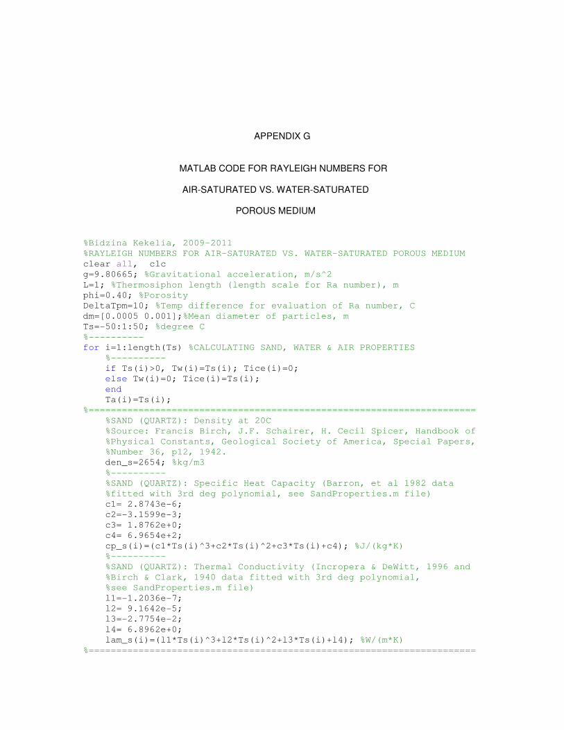
APPENDIX G
G - MATLAB CODE FOR RAYLEIGH NUMBERS FOR
AIR-SATURATED VS. WATER-SATURATED
POROUS MEDIUM
%Bidzina Kekelia, 2009-2011 %RAYLEIGH NUMBERS FOR AIR-SATURATED VS. WATER-SATURATED POROUS MEDIUM clear all, clc g=9.80665; %Gravitational acceleration, m/s^2 L=1; %Thermosiphon length (length scale for Ra number), m phi=0.40; %Porosity DeltaTpm=10; %Temp difference for evaluation of Ra number, C dm=[0.0005 0.001];%Mean diameter of particles, m Ts=-50:1:50; %degree C %---------- for i=1:length(Ts) %CALCULATING SAND, WATER & AIR PROPERTIES %---------- if Ts(i)>0, Tw(i)=Ts(i); Tice(i)=0; else Tw(i)=0; Tice(i)=Ts(i); end Ta(i)=Ts(i); %====================================================================== %SAND (QUARTZ): Density at 20C %Source: Francis Birch, J.F. Schairer, H. Cecil Spicer, Handbook of %Physical Constants, Geological Society of America, Special Papers, %Number 36, p12, 1942. den_s=2654; %kg/m3 %---------- %SAND (QUARTZ): Specific Heat Capacity (Barron, et al 1982 data
%fitted with 3rd deg polynomial, see SandProperties.m file) c1= 2.8743e-6; c2=-3.1599e-3; c3= 1.8762e+0; c4= 6.9654e+2; cp_s(i)=(c1*Ts(i)^3+c2*Ts(i)^2+c3*Ts(i)+c4); %J/(kg*K) %---------- %SAND (QUARTZ): Thermal Conductivity (Incropera & DeWitt, 1996 and %Birch & Clark, 1940 data fitted with 3rd deg polynomial, %see SandProperties.m file) l1=-1.2036e-7; l2= 9.1642e-5; l3=-2.7754e-2; l4= 6.8962e+0; lam_s(i)=(l1*Ts(i)^3+l2*Ts(i)^2+l3*Ts(i)+l4); %W/(m*K) %======================================================================

196
%WATER: Density - Source: Metrologia, 2001, 38, pp301-309. a1=-3.983035; a2=301.797; a3=522528.9; a4=69.34881; a5=999.974950; den_w(i)=a5*(1-(Tw(i)+a1)^2*(Tw(i)+a2)/(a3*(Tw(i)+a4))); %kg/m^3 %---------- %WATER: Dynamic Viscosity: miu(Pa·s)=A×10^(B/(T-C)) %Source: http://en.wikipedia.org/wiki/Viscosity#Viscosity_of_water miu_w(i)=2.414e-5*10^(247.8/(Tw(i)+273-140)); %Pa*s %---------- %WATER: Kinematic Viscosity niu_w(i)=miu_w(i)/den_w(i); %m^2/s %---------- %WATER: Thermal Expansion Coefficient (Curve fitted 4th deg
polynomial) %(see Waterproperties_combined.m file) b1=-1.9992e-11; b2= 3.4724e-9; b3=-2.7200e-7; b4= 1.7933e-5; b5=-6.7470e-5; beta_w(i)=b1*Tw(i)^4+b2*Tw(i)^3+b3*Tw(i)^2+b4*Tw(i)+b5; %m^3/C %---------- %WATER: Specific Heat Capacity (NIST data fitted with 4th deg
polynom.) %(see Waterproperties_combined.m file) c1= 9.8933e-9; c2=-1.5591e-6; c3= 1.0407e-4; c4=-3.2972e-3; c5= 4.2192e+0; cp_w(i)=(c1*Tw(i)^4+c2*Tw(i)^3+c3*Tw(i)^2+c4*Tw(i)+c5)*10^3;
%J/(kg*K) %---------- %WATER: Thermal Conductivity (NIST data fitted with 4th deg
polynomial) %(see Waterproperties_combined.m file) l1= 1.1942e-9; l2=-2.0865e-7; l3= 2.6531e-6; l4= 1.8900e-3; l5= 5.6108e-1; lam_w(i)=l1*Tw(i)^4+l2*Tw(i)^3+l3*Tw(i)^2+l4*Tw(i)+l5; %W/(m*K) %====================================================================== %ICE: Density at 1 atm (CRC Handbook data fitted 3rd deg polynom) %2010-2011 CRC Handbook of Chemistry and Physics, 91st ed., p.6-12. %(see Iceproperties_Celcius.m file) ai1= 7.6944e-007; ai2=-1.7506e-004; ai3=-1.4600e-001; ai4= 9.1673e+002; den_ice(i)=ai1*Tice(i)^3+ai2*Tice(i)^2+ai3*Tice(i)+ai4; %kg/m^3 %---------- %ICE: Specific Heat Capacity, cp (CRC Handbook data fitted 3rd deg %polynomial), (see Iceproperties_Celcius.m file)

197
ci1= 1.3642e-005; ci2= 5.4463e-003; ci3= 7.5938e+000; ci4= 2.0988e+003; cp_ice(i)=ci1*Tice(i)^3+ci2*Tice(i)^2+ci3*Tice(i)+ci4; %J/kg*K %---------- %ICE: Thermal Conductivity (CRC Handbook data fitted with 3rd deg %polynomial), (see Iceproperties_Celcius.m file) li1=-2.3838e-007; li2= 2.4879e-005; li3=-1.0440e-002; li4= 2.1576e+000; lam_ice(i)=li1*Tice(i)^3+li2*Tice(i)^2+li3*Tice(i)+li4; %W/(m*K) %====================================================================== %AIR: Density at 1 atm (Curve fitted 3rd deg polynomial) %(see Airproperties_1atm_Celcius.m file) aa1=-3.8521e-008; aa2= 1.9307e-005; aa3=-5.0075e-003; aa4= 1.2915e+000; den_a(i)=aa1*Ta(i)^3+aa2*Ta(i)^2+aa3*Ta(i)+aa4; %kg/m^3 %---------- %AIR: Dynamic Viscosity (Curve fitted 3rd deg polynomial) %(see Airproperties_1atm_Celcius.m file) m1= 4.1045e-014; m2=-4.2884e-011; m3= 4.9708e-008; m4= 1.7153e-005; miu_a(i)=m1*Ta(i)^3+m2*Ta(i)^2+m3*Ta(i)+m4; %Pa*s %---------- %AIR: Kinematic Viscosity niu_a(i)=miu_a(i)/den_a(i); %m^2/s %---------- %AIR: Specific Heat Capacity, cp %(see Airproperties_1atm_Celcius.m file) ca1= 3.0166e-007; ca2= 2.7138e-004; ca3= 3.6770e-002; ca4= 1.0037e+003; cp_a(i)=ca1*Ta(i)^3+ca2*Ta(i)^2+ca3*Ta(i)+ca4; %J/kg*K %---------- %AIR: Thermal Conductivity, lambda %(see Airproperties_1atm_Celcius.m file) la1= 1.6442e-011; la2=-3.8493e-008; la3= 7.9654e-005; la4= 2.4119e-002; lam_a(i)=la1*Ta(i)^3+la2*Ta(i)^2+la3*Ta(i)+la4; %W/m*K %---------- %AIR: Thermal Expansion Coefficient, beta %(see Airproperties_1atm_Celcius.m file) ba1= 3.0093e-010; ba2=-2.4851e-008; ba3=-1.4982e-005; ba4= 3.8770e-003; beta_a(i)=ba1*Ta(i)^3+ba2*Ta(i)^2+ba3*Ta(i)+ba4; %1/K %======================================================================

198
%PM: Thermal Conductivity using power law combination of
%min(serial) and max(parallel) conduction models (Chaudhary &
%Bhandari, 1968) n=0.4; %Weighting factor (taken arbitrarily as exact value unknown) lam_max_w=phi*lam_w(i)+(1-phi)*lam_s(i); %Parallel model for water lam_min_w=lam_s(i)*lam_w(i)/(phi*lam_s(i)+(1-phi)*lam_w(i));%Series lam_pm_w(i)=lam_max_w^n*lam_min_w^(1-n); %WATER-saturated, W/(m*K) lam_max_ice=phi*lam_ice(i)+(1-phi)*lam_s(i);%Parallel model for ice lam_min_ice=lam_s(i)*lam_ice(i)/(phi*lam_s(i)+(1-phi)*lam_ice(i));
%Series lam_pm_ice(i)=lam_max_ice^n*lam_min_ice^(1-n);%ICE-sat, W/(m*K) lam_max_a=phi*lam_a(i)+(1-phi)*lam_s(i); %Parallel model for air lam_min_a=lam_s(i)*lam_a(i)/(phi*lam_s(i)+(1-phi)*lam_a(i));%Series
air lam_pm_a(i)=lam_max_a^n*lam_min_a^(1-n); %AIR-saturated, W/(m*K) %---------- %PM: Volumetric heat capacity (energy stored in unit vol. of PM) ED_sand(i)=(1-phi)*den_s*cp_s(i); ED_water(i)=phi*den_w(i)*cp_w(i); ED_ice(i)=phi*den_ice(i)*cp_ice(i); ED_air(i)=phi*den_a(i)*cp_a(i); ED_pm_w(i)=ED_water(i)+ED_sand(i); %WATER-saturated, J/m^3*K ED_pm_ice(i)=ED_ice(i)+ED_sand(i); %ICE-saturated, J/m^3*K ED_pm_a(i)=ED_air(i)+ED_sand(i); %AIR-saturated, J/m^3*K %---------- %PM: Thermal diffusivity of PM alpha_pm_w(i)=lam_pm_w(i)/ED_pm_w(i); %WATER-saturated, m^2/s alpha_pm_ice(i)=lam_pm_ice(i)/ED_pm_ice(i); %ICE-saturated, m^2/s alpha_pm_a(i)=lam_pm_a(i)/ED_pm_a(i); %AIR-saturated, m^2/s end for j=1:length(dm) %Number of grain sizes (and respective
permeabilities k_pm(j)=dm(j)^2*phi^3/(180*(1-phi)^2); %Permeability (Kozeny eq.) for i=1:length(Ts) %================================================================= %CALCULATING RAYLEIGH NUMBER: Ra_w(i,j)=g*beta_w(i)*DeltaTpm*L*k_pm(j)/(niu_w(i)*alpha_pm_w(i)); Ra_a(i,j)=g*beta_a(i)*DeltaTpm*L*k_pm(j)/(niu_a(i)*alpha_pm_a(i)); %================================================================= end end figure(11) plot(Tw,Ra_w(:,1),'b',Tw,Ra_w(:,2),'b','LineWidth',2),hold on,grid on plot(Ta,Ra_a(:,1),'m',Ta,Ra_a(:,2),'m','LineWidth',2) xlabel('T (\circC)'), ylabel('Ra_pm'); xlim([-50 50]) ylim([-10 150]) %title(['Rayleigh numbers for Water- vs. Air-Saturated PM'],... % ['\itL = ',num2str(L,'%10.1f'),... % 'm, \phi = ',num2str(phi*100,'%10.0f'),... % '%, \DeltaT = ',num2str(DeltaTpm,'%10.0f'),'\circC']) legend(['Ra_w, d_m= ',num2str(dm(1)*1000,'%10.1f'),... 'mm, k_p_m= ',num2str(k_pm(1),'%10.1e'),'m^2'],... ['Ra_w, d_m= ',num2str(dm(2)*1000,'%10.1f'),... 'mm, k_p_m= ',num2str(k_pm(2),'%10.1e'),'m^2'],... ['Ra_a, d_m= ',num2str(dm(1)*1000,'%10.1f'),... 'mm, k_p_m= ',num2str(k_pm(1),'%10.1e'),'m^2'],...

199
['Ra_a, d_m= ',num2str(dm(2)*1000,'%10.1f'),... 'mm, k_p_m= ',num2str(k_pm(2),'%10.1e'),'m^2'],... 'Location','W') for j=1:length(dm) text(Tw(99),Ra_w(99,j),... ['Ra_w, d_m=',num2str(dm(j)*1000,'%10.1f'),'mm '],... 'HorizontalAlignment','right') text(Ta(25),Ra_a(25,j)+2,... ['Ra_a, d_m=',num2str(dm(j)*1000,'%10.1f'),'mm']) end
figure(12) plot(Tw,niu_w,'b',Ta,niu_a,'m','LineWidth',2), grid on xlabel('T (\circC)'), ylabel('\nu (m^2/s)'); xlim([-50,50]) ylim([0,1.8e-5]) %title('Kinematic viscosities of air and water') text(Tw(60),niu_w(1),' \nu_water') text(Ta(60),niu_a(70),' \nu_air')
figure(13) plot(Tw,beta_w,'b',Ta,beta_a,'m','LineWidth',2), grid on xlabel('T (\circC)'), ylabel('\beta (1/K)'); xlim([-50,50]) ylim([-0.1e-3,4.5e-3]) %title('Thermal expansion coefficients of air and water') text(Tw(62),beta_w(85),'\beta_water') text(Ta(62),beta_a(55),'\beta_air')
figure(14) plot(Tw,lam_pm_w,'b',Tice,lam_pm_ice,'b',Ta,lam_pm_a,'m',... 'LineWidth',2),grid on xlabel('T (\circC)') ylabel('\lambda_p_m (W/m\cdotK)'); xlim([-50,50]) ylim([-0,5.5]) %title('Thermal conductivities') text(Tw(62),lam_pm_w(62)+0.2,'\lambda_pm water') text(Tice(22),lam_pm_ice(22)+0.2,'\lambda_pm ice') text(Ta(62),lam_pm_a(62)+0.2,'\lambda_pm air')
figure(15) plot(Tw,ED_pm_w,'b',Tice,ED_pm_ice,'b',Ta,ED_pm_a,'m',... 'LineWidth',2), grid on xlabel('T (\circC)') ylabel('C_pm (J/m^3\cdotK)'); xlim([-50,50]) %title('Volumetric heat capacity of PM') text(Tw(62),ED_pm_w(62)+10^5,'C_pm water') text(Tice(22),ED_pm_ice(22)+1.5*10^5,'C_pm ice') text(Ta(62),ED_pm_a(62)+1.1*10^5,'C_pm air')
figure(16) plot(Tw,alpha_pm_w,'b',Tice,alpha_pm_ice,'b',Ta,alpha_pm_a,'m',... 'LineWidth',2), grid on xlabel('T (\circC)')

200
ylabel('\alpha_p_m (m^2/s)'); xlim([-50,50]) %title('Thermal diffusivities') text(Tw(62),alpha_pm_w(62)+10^-7,'\alpha_pm water') text(Tice(22),alpha_pm_ice(22)+8*10^-8,'\alpha_pm ice') text(Ta(62),alpha_pm_a(62)+10^-7,'\alpha_pm air')