The One Dimensional Heat EquationKurt Bryan

1 Informal Derivation in One Dimension

Consider a one-dimensional “bar” lying along the x axis from x = 0 tox = 1. Let t denote time and u(t, x) the temperature of the bar at time tand position x. We want to find an equation that governs the temperatureu in the interior of the bar. In what follows we’ll use the notation ux for ∂u

∂x,

uxx = ∂2u∂x2 , etc.

We’ll think of u as a measurement of the density of “thermal energy”in the bar. Specifically, consider a portion of the bar stretching from x tox + ∆x, where ∆x is small; we’ll refer to this part of the bar as the “controlvolume”. We’ll assume that the amount of thermal energy in the controlvolume is given approximately by cu(t, x)∆x where c is some constant. Notethat cu(t, x)∆x has dimensions of energy. The constant c is related to thespecific heat of the material out of which the bar is made.

It’s intuitively clear that heat energy flows from hotter regions to colderregions. We’ll assume that the rate at which energy flows through or past apoint x from left to right (increasing x) in the bar is given by −α(x)ux(t, x),where α(x) > 0 is some function, called the thermal conductivity of the barat point x. If the bar is homogeneous (most typical) then α(x) is actuallya constant. The quantity −α(x)ux(t, x) has dimension energy per time, andthe flow of thermal energy is “downhill”, from hot to cold, since −α(x) < 0.We’ll require that α(x) be twice continuously differentiable for now.

Now we’ll invoke conservation of energy: The rate at which energy flowsINTO the left end of the control volume is given by −α(x)ux(t, x) (make sureyou believe the sign is correct). The rate at which energy flows INTO theright end of the control volume is given by α(x + ∆x)ux(t, x + ∆x) (again,make sure you believe the sign is correct). All in all thermal energy is flowinginto the control volume at a rate of

rate in = α(x + ∆x) (ux(t, x + ∆x)− α(x)ux(t, x)) . (1)

But by conservation of energy this means that the thermal energy in thecontrol volume is increasing at this rate. The rate at which the total energyof the control volume increases is given by

rate of increase ≈ cut(t, x)∆x (2)

1

If we equate the right sides of equations (1) and (2), divide by ∆x, and let∆x approach zero we find that u(t, x) should satisfy

ut − (κ(x)ux)x = 0, (3)

the so-called heat equation, where κ(x) = α(x)c

is called the thermal diffusivityof the bar. For simplicity we’ll often take κ = 1.

The heat equation requires boundary and initial conditions in order topossess a unique solution. One typically specifies and initial conditions likeu(0, x) = u0(x) for some specified initial temperature u0(x). For the bound-ary conditions at the endpoints one possibility is to specify u(t, 0) = f0(t)and u(t, 1) = f1(t) (so the endpoint temperatures are specified, so-calledDirichlet boundary conditions). Or one can specify the rate at which heatenergy is entering the ends of the bar. This leads to boundary conditions−α(0)ux(t, 0) = g0(t) and α(1)ux(t, 1) = g1(t) (these are the Neumannboundary conditions). If gi(t) ≡ 0 for i = 0 or i = 1 then we have aninsulating boundary condition at that end of the bar.

One can show that under reasonable assumptions on the initial temper-ature u0 and boundary conditions f0 and f1, or g0 and g1, the heat equationhas a unique solution.

2 Modeling Defects: The Forward Problem

Consider a one-dimensional bar stretching from x = 0 to x = 1. For sim-plicity let’s take the constants above to be one, so α = c = κ = 1. Withu(t, x) denoting the temperature in the bar we should have ut − uxx = 0 for0 < x < 1 and t > 0, with appropriate boundary and initial conditions.

But suppose that the bar contains an interior point “defect”, that is, somepoint x = σ with 0 < σ < 1 in the interior of the bar through which theflow of heat is somehow impeded. For example, at x = σ there might be a“break” in the bar which blocks the flow of heat. At that point we’d haveux(t, σ) = 0 for all t. But more generally, we can consider a defect whichallows heat to flow past x = σ, but with some “resistance”.

To quantify this, let’s define notation

u−(t) = limx→σ−

u(t, x), u+(t) = limx→σ+

u(t, x),

u−x (t) = limx→σ−

ux(t, x), u+x (t) = lim

x→σ+ux(t, x),

2

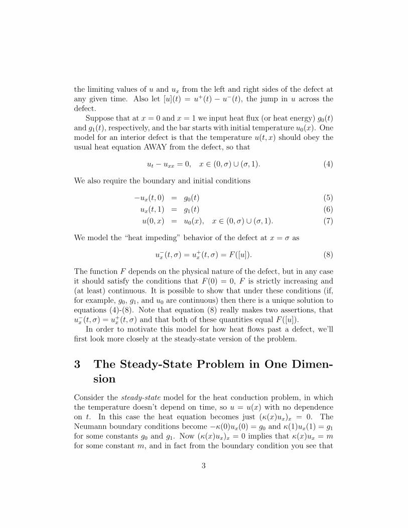
the limiting values of u and ux from the left and right sides of the defect atany given time. Also let [u](t) = u+(t) − u−(t), the jump in u across thedefect.

Suppose that at x = 0 and x = 1 we input heat flux (or heat energy) g0(t)and g1(t), respectively, and the bar starts with initial temperature u0(x). Onemodel for an interior defect is that the temperature u(t, x) should obey theusual heat equation AWAY from the defect, so that

ut − uxx = 0, x ∈ (0, σ) ∪ (σ, 1). (4)

We also require the boundary and initial conditions

−ux(t, 0) = g0(t) (5)

ux(t, 1) = g1(t) (6)

u(0, x) = u0(x), x ∈ (0, σ) ∪ (σ, 1). (7)

We model the “heat impeding” behavior of the defect at x = σ as

u−x (t, σ) = u+x (t, σ) = F ([u]). (8)

The function F depends on the physical nature of the defect, but in any caseit should satisfy the conditions that F (0) = 0, F is strictly increasing and(at least) continuous. It is possible to show that under these conditions (if,for example, g0, g1, and u0 are continuous) then there is a unique solution toequations (4)-(8). Note that equation (8) really makes two assertions, thatu−x (t, σ) = u+

x (t, σ) and that both of these quantities equal F ([u]).In order to motivate this model for how heat flows past a defect, we’ll

first look more closely at the steady-state version of the problem.

3 The Steady-State Problem in One Dimen-

sion

Consider the steady-state model for the heat conduction problem, in whichthe temperature doesn’t depend on time, so u = u(x) with no dependenceon t. In this case the heat equation becomes just (κ(x)ux)x = 0. TheNeumann boundary conditions become −κ(0)ux(0) = g0 and κ(1)ux(1) = g1

for some constants g0 and g1. Now (κ(x)ux)x = 0 implies that κ(x)ux = mfor some constant m, and in fact from the boundary condition you see that

3

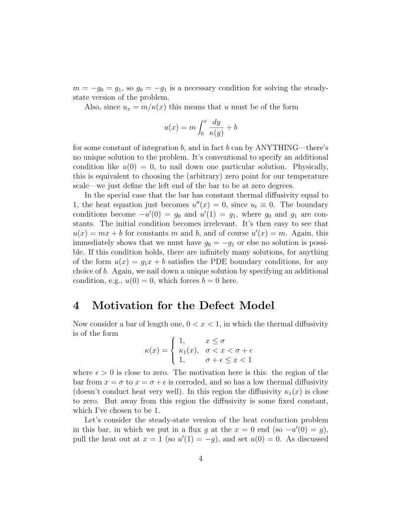
m = −g0 = g1, so g0 = −g1 is a necessary condition for solving the steady-state version of the problem.

Also, since ux = m/κ(x) this means that u must be of the form

u(x) = m∫ x

0

dy

κ(y)+ b

for some constant of integration b, and in fact b can by ANYTHING—there’sno unique solution to the problem. It’s conventional to specify an additionalcondition like u(0) = 0, to nail down one particular solution. Physically,this is equivalent to choosing the (arbitrary) zero point for our temperaturescale—we just define the left end of the bar to be at zero degrees.

In the special case that the bar has constant thermal diffusivity equal to1, the heat equation just becomes u′′(x) = 0, since ut ≡ 0. The boundaryconditions become −u′(0) = g0 and u′(1) = g1, where g0 and g1 are con-stants. The initial condition becomes irrelevant. It’s then easy to see thatu(x) = mx + b for constants m and b, and of course u′(x) = m. Again, thisimmediately shows that we must have g0 = −g1 or else no solution is possi-ble. If this condition holds, there are infinitely many solutions, for anythingof the form u(x) = g1x + b satisfies the PDE boundary conditions, for anychoice of b. Again, we nail down a unique solution by specifying an additionalcondition, e.g., u(0) = 0, which forces b = 0 here.

4 Motivation for the Defect Model

Now consider a bar of length one, 0 < x < 1, in which the thermal diffusivityis of the form

κ(x) =

1, x ≤ σκ1(x), σ < x < σ + ε1, σ + ε ≤ x < 1

where ε > 0 is close to zero. The motivation here is this: the region of thebar from x = σ to x = σ + ε is corroded, and so has a low thermal diffusivity(doesn’t conduct heat very well). In this region the diffusivity κ1(x) is closeto zero. But away from this region the diffusivity is some fixed constant,which I’ve chosen to be 1.

Let’s consider the steady-state version of the heat conduction problemin this bar, in which we put in a flux g at the x = 0 end (so −u′(0) = g),pull the heat out at x = 1 (so u′(1) = −g), and set u(0) = 0. As discussed

4

above, from the steady-state heat equation (κ(x)ux)x = 0 we have, from oneintegration,

u′(x) = − g

κ(x), (9)

and a second integral gives

u(x) = u(0)−∫ x

0

g

κ(y)dy. (10)

It’s easy to see from equation (9) that away from the defect region wehave u′(x) = −g. But within the defect region we have u′(x) = −g/κ(x),which is of much greater magnitude than −g, since κ(x) > 0 is close to zero,except maybe at the edges near x = σ and x = σ + ε. The solution will looksomething like this:

In fact, if we assume that κ(x) ≈ κ0 (a constant) in the defect region, thenu′(x) = − g

κ0in this region. As a result, the solution will rise a distance of

−g εκ0

in the short space from x = σ to x = σ + ε. Note that u′ = −g,however, just outside either boundary of the defect.

The inverse problem would be to recover the defect, defined by its leftboundary σ, right boundary σ + ε, and diffusivity profile κ1(x). But in fact,we probably wouldn’t be interested in the precise profile of the corrosiondiffusivity, but rather it’s rough location (σ) and overall magnitude. Thusinstead of modelling the defect as above, we could consider it to be a “point”within the bar, at x = σ. Instead of worrying about the diffusivity of thedefect, we simply capture it’s behavior with the requirement that u′(x) havethe same limiting value on both side of σ, and that u have an appropriate

5

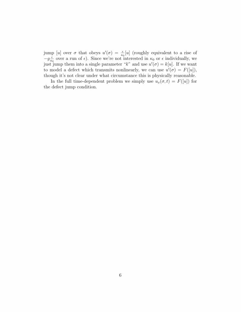
jump [u] over σ that obeys u′(σ) = εκ0

[u] (roughly equivalent to a rise of−g ε

κ0over a run of ε). Since we’re not interested in κ0 or ε individually, we

just jump them into a single parameter “k” and use u′(σ) = k[u]. If we wantto model a defect which transmits nonlinearly, we can use u′(σ) = F ([u]),though it’s not clear under what circumstance this is physically reasonable.

In the full time-dependent problem we simply use ux(σ, t) = F ([u]) forthe defect jump condition.

6