hecke l-functions, eisenstein series, and the distribution … · hecke l-functions, eisenstein...
TRANSCRIPT

HECKE L-FUNCTIONS, EISENSTEIN SERIES, AND THE
DISTRIBUTION OF TOTALLY POSITIVE INTEGERS
by Avner Ash and Solomon Friedberg
Boston College
June 2004
Abstract. Let K be a number field of degree n. We show that the maximal parabolicEisenstein series on GL(n), restricted to the non-split torus obtained from K, has a Fourier
expansion, and that the Fourier coefficients may be expressed in terms of Hecke L-functions.This is an analogue of the computation of the classical hyperbolic expansion of the GL(2)
nonholomorphic Eisenstein series. We also show that if K is totally real then the number of
totally positive integers (or more generally the number of totally positive elements of a givenfractional ideal) of given trace is evenly distributed around its expected value. These results
both depend on unfolding an integral over a compact torus.
0. Introduction
In 1921 Hecke published the paper “Uber analytische Funktionen und die Verteilung vonZahlen mod. Eins” [He]. In it, he showed (among other things) that the Fourier coefficientsof certain functions on a non-split torus in GL(2)/Q were given by (what we now call) theL-functions of certain Hecke characters of a real quadratic field. Interestingly, the Heckecharacters which arise here are not of type A.
Hecke’s key idea in that portion of his paper is to unfold the integral that computes theFourier coefficient in a manner foreshadowing the Rankin-Selberg method. Siegel, in hisbook Advanced Analytic Number Theory [Si, Ch. II, Section 4] observed that the samemethod could be used to compute the hyperbolic Fourier expansion of the nonholomor-phic Eisenstein series on GL(2)/Q, and to express these coefficients in terms of HeckeL-functions.
Hecke used his Fourier expansion to study the distribution of the fractional parts ofmα where m runs over the rational integers and α is a fixed real quadratic irrationality.
1991 Mathematics Subject Classification. Primary 11M41, Secondary 11F30, 11F55, 11H06, 11R47.Key words and phrases. Eisenstein series, toroidal integral, Fourier series, Hecke L-function, totally
positive integer, trace.
Research supported in part by NSF grant DMS-0139287 (Ash) and by NSA grant MDA904-03-1-0012(Friedberg).
Typeset by AMS-TEX
1

2 AVNER ASH AND SOLOMON FRIEDBERG
Siegel used his in conjunction with Kronecker’s limit formula to derive some relationshipsbetween Dedekind’s η-function and invariants of real quadratic fields.
In this paper, we first generalize Siegel’s Fourier expansion computation to GL(n)/Q.Where Siegel worked with a real quadratic field, we let K be any number field, [K : Q] = n.We can view K as the Q-points of a non-split torus T in GL(n)/Q. Let X denote thetotally geodesic subspace of the symmetric space of GL(n)/Q defined by T . We find theFourier expansion of the restriction to X of the standard maximal parabolic Eisensteinseries E(g, s) of type (n − 1, 1). We prove that the Fourier coefficients, which are againfunctions of s, are in fact certain Hecke L-functions associated to K (more accurately,partial Hecke L-functions with respect to a certain ideal class in K). In particular, theconstant term of the Fourier expansion is given by the partial zeta-function of K. This hasalready been proven adelically by Wielonsky [Wi1, Wi2]. We do not pursue this further,although no doubt analogues to the η-function could be introduced in conjunction withthe generalization to GL(n) of Kronecker’s limit formula. This has been done by Efrat[Ef] for GL(3); see also Bump and Goldfeld [B-G].
Next we assume that K is totally real and use the Fourier expansion to generalize oneof Hecke’s results on the distribution of fractional parts. The correct generalization of thefractional part of mα turns out to be the error term in the natural geometric estimatefor the number of integers of K of a given trace. We form the Dirichlet series ϕ(s) whosecoefficients are these errors.
More specifically, let a denote a fractional ideal in the ring of integers of K, and let Tr(a)be generated by k > 0. If a is a positive integral multiple of k, let Na denote the numberof totally positive elements of a with trace a. There is the natural geometric estimate ra
of Na derived from the volume of the intersection in a ⊗ R of the cone of totally positiveelements with the hyperplane defined by Trace = a. Denote the difference between Na andits estimate as a volume by Ea: Ea = Na − ra. Note that Ea may be positive or negative.If a is not a positive multiple of k, we set Ea = 0.
Define the Dirichlet seriesϕ(s) =
∑a>0
Ea
as.
The analytic properties of ϕ(s) are related to the distribution of the errors Ea in theusual way of analytic number theory. The natural estimate on the size of the errors,obtained from standard results concerning the counting of lattice points in a homogeneouslyexpanding domain, gives us that ϕ(s) is (absolutely) convergent for <(s) > n−1. It followsthat ∑
a<X
Ea � Xn−1.
Any improvement of this abscissa of convergence implies a corresponding improvement inthe estimate for
∑a<X Ea which measures the evenness of the distribution of these errors
about 0.Following Hecke, we express ϕ(s) in terms of a zeta-function and a function whose
Fourier series over the non-split torus we can compute. The Fourier coefficients are onceagain related to Hecke L-functions not of type A. From this expression, we deduce that

HECKE L-FUNCTIONS, EISENSTEIN SERIES, AND TOTALLY POSITIVE INTEGERS 3
ϕ(s) can be continued to a regular function in the right half plane <(s) > 0. Here we noticean important difference with Hecke’s case n = 2. Namely, the Gamma factors, which inHecke’s case caused ϕ(s) to be meromorphic with known poles, in our case give densesets of poles which prevent the continuation of ϕ(s) to left of the line <(s) = 0. That is,each term in the Fourier expansion is an L-function times a Gamma factor with infinitelymany poles, but the poles become dense along certain vertical lines when we sum up allthe terms. Nevertheless, we can use the functional equation of each term separately plusStirling’s formula to study the behavior of ϕ(s) in vertical strips to the right of <(s) = 0.This enables us to use a Theorem of Schnee and Landau to conclude that ϕ(s) convergesfor <(s) > n− 1− (2n− 2)/(2n + 1).
Our main result then follows by summation by parts:
Main Theorem. For ε > 0, ∑a<X
Ea = O(Xn−1− 2n−2
2n+1 +ε)
.
When n = 2, Hecke gets the bound O(Xε), because he is able to exploit (in a complicatedway) the fact that his ϕ(s) has a meromorphic continuation to the whole s-plane. Althoughour bound is not as good – one might expect O(Xn−2+ε) as the correct generalization –note that the exponent in our bound does approach n− 2 as n goes to infinity.
Another recent generalization of these ideas of Hecke, in this case to certain ellipticalcones, may be found in Duke-Immamoglu [D-I]. Also, Chinta and Goldfeld [C-G] haveused Siegel’s computation in the case of Eisenstein series involving a modular symbol tocontinue a Dirichlet series which is the twist of a Hecke L-function by a modular symbol.Once again, though we do not pursue it here, it is reasonable to expect that our methodsmay allow one to generalize this construction.
The remainder of this paper is organized as follows. Section 1 explains how one maygeneralize the classical hyperbolic Fourier expansion to a toroidal Fourier expansion of anautomorphic form on GL(n). Section 2 introduces the maximal parabolic Eisenstein serieson GL(n) of type (n− 1, 1); in Section 3 the toroidal Fourier coefficients of this Eisensteinseries are expressed in terms of Hecke L-functions for K. For the remaining sections, wesuppose that K is totally real. In Section 4, we introduce a family of Dirichlet serieswhich are functions of n− 1 positive variables yi as well as the complex parameter s. Weshow that these functions have Fourier expansions in the yi similar to the toroidal Fourierexpansion above, compute their Fourier coefficients, and show that they have continuationin s. In Section 5 we obtain a formula (Proposition 5.1) for the quantity ra, the naturalestimate for the number of totally positive integers in a given fractional ideal a which are oftrace a, using geometric methods. Section 6 begins our study of the Dirichlet series ϕ(s).Combining the geometry and the analysis of the previous two sections, we show that ϕ(s) isholomorphic for <(s) > 0. In the last two sections we carry out an analysis of the growthof ϕ(s) in vertical strips in <(s) > 0. Section 7 contains some geometric preliminariesconcerning the number of points in the intersection of a lattice with a certain family ofcompact polyhedra. In Section 8 we use the Fourier expansion of Section 4 together with

4 AVNER ASH AND SOLOMON FRIEDBERG
Stirling’s formula and the geometric information of Section 7 in order to obtain an estimateon the growth of ϕ(s). From this information we obtain the main theorem above.
1. Toroidal Fourier Expansions on GL(n)
In this section we develop a Fourier expansion on GL(n) which is the analogue of theclassical hyperbolic expansion on GL(2). We describe this as a toroidal Fourier expansionto indicate that it is separate from the usual Fourier expansion which arises in the theoryof automorphic forms.
Let K be a number field, [K : Q] = n, with r1 real embeddings σk : K → R, 1 ≤ k ≤ r1,and 2r2 complex embeddings σr1+k : K → C, 1 ≤ k ≤ 2r2. Set r = r1+r2−1, and supposer > 0. Order the complex embeddings so that σr1+2j = σr1+2j−1 for 1 ≤ j ≤ r2; then thearchimedean places of K are indexed by the set I = {k | 1 ≤ k ≤ r1 or k = r1 +2j−1, 1 ≤j ≤ r2}. For α ∈ K and 1 ≤ k ≤ n, let α(k) = σk(α), and let
α(k) ={
σk(α) 1 ≤ k ≤ r1
(ak, bk) where σk(α) = ak + bki, k = r1 + 1, r1 + 3, · · · , n− 1
α(k) =
σk(α) 1 ≤ k ≤ r1(
ak bk
−bk ak
)where σk(α) = ak + bki, k = r1 + 1, r1 + 3, · · · , n− 1.
Let ε1, · · · , εr be units which together with the roots of unity in K generate the fullgroup of units in K. Let b be a fractional ideal of K with Z-basis ω1, · · · , ωn, and let φ
denote the n× n matrix φ = (ω(j)i ), 1 ≤ i ≤ n, j ∈ I. Then
(1.1) |detφ| = (disc b)1/2 2−r2 ,
where disc b denotes the absolute discriminant. There are matrices ρ` ∈ GL(n, Z), 1 ≤ ` ≤r, such that ρ`φ = φE` where E` ∈ GL(n, Z) is given by
E` = diag(ε(1)` , · · · , ε
(r1)` , ε
(r1+1)` , ε
(r1+3)` , · · · , ε
(n−1)`
).
Indeed, φE` is of the form (β(j)i ), 1 ≤ i ≤ n, j ∈ I with βi = ωiε` ∈ b, and the matrix ρ`
gives the βi in terms of the basis {ωj}.Let F (g) be an automorphic form on GL(n, AQ), not necessarily cuspidal. For simplicity
let us suppose that in fact F (g) has trivial central character, is K-fixed, and is of level1. Let H = GL(n, R)/ZO(n) be the symmetric space of GL(n, R); here Z denotes thecenter consisting of scalar matrices and O(n) is the real orthogonal group. By the Iwasawadecomposition, each coset is represented by an upper triangular matrix τ with (n, n)-entry1. We write the natural action of GL(n, R) on H as γ ◦ τ . Then F corresponds to afunction f : H → C such that f(γ ◦ τ) = f(τ) for all γ ∈ GL(n, Z).
Let T be the torus in H consisting of y = diag(y1, · · · , yn−1, 1) such that (if r2 > 0)yr1+2j = yr1+2j−1 for 1 ≤ j ≤ r2. Let X = φ ◦ T . Then X is a totally geodesic subspace
HECKE L-FUNCTIONS, EISENSTEIN SERIES, AND TOTALLY POSITIVE INTEGERS 5
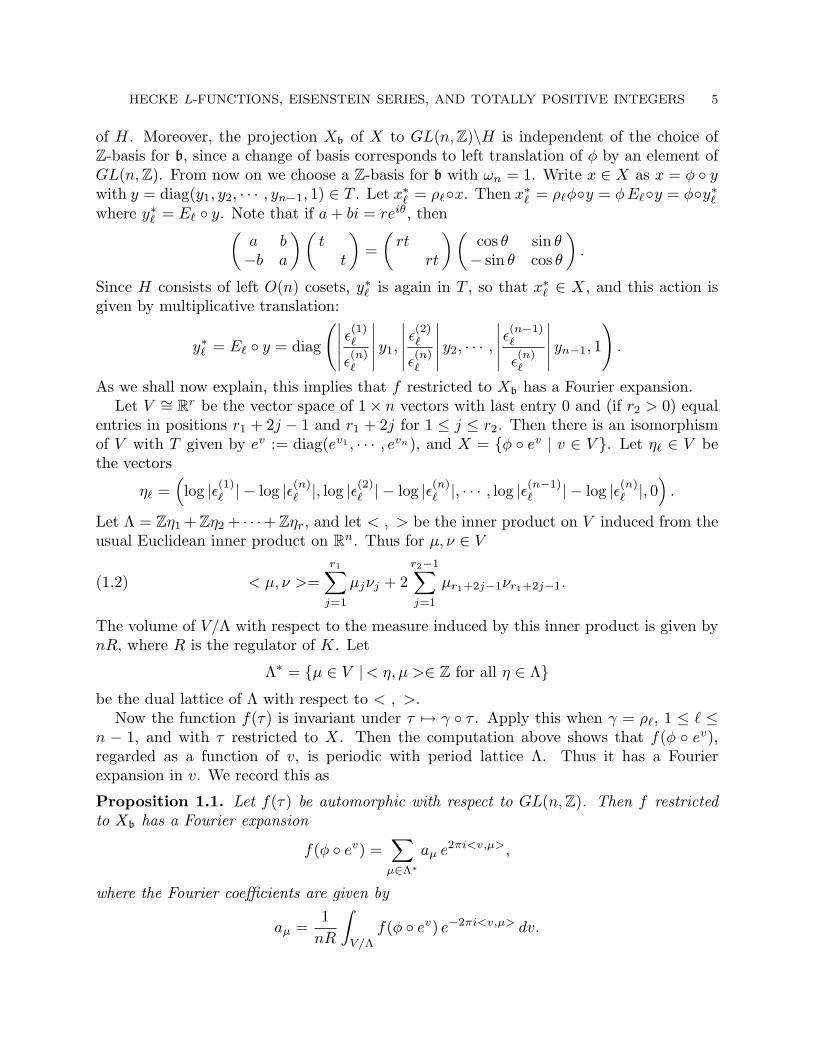
of H. Moreover, the projection Xb of X to GL(n, Z)\H is independent of the choice ofZ-basis for b, since a change of basis corresponds to left translation of φ by an element ofGL(n, Z). From now on we choose a Z-basis for b with ωn = 1. Write x ∈ X as x = φ ◦ ywith y = diag(y1, y2, · · · , yn−1, 1) ∈ T . Let x∗` = ρ`◦x. Then x∗` = ρ`φ◦y = φ E`◦y = φ◦y∗`where y∗` = E` ◦ y. Note that if a + bi = reiθ, then(
a b−b a
)(t
t
)=(
rtrt
)(cos θ sin θ− sin θ cos θ
).
Since H consists of left O(n) cosets, y∗` is again in T , so that x∗` ∈ X, and this action isgiven by multiplicative translation:
y∗` = E` ◦ y = diag
(∣∣∣∣∣ ε(1)`
ε(n)`
∣∣∣∣∣ y1,
∣∣∣∣∣ ε(2)`
ε(n)`
∣∣∣∣∣ y2, · · · ,
∣∣∣∣∣ε(n−1)`
ε(n)`
∣∣∣∣∣ yn−1, 1
).
As we shall now explain, this implies that f restricted to Xb has a Fourier expansion.Let V ∼= Rr be the vector space of 1× n vectors with last entry 0 and (if r2 > 0) equal
entries in positions r1 + 2j − 1 and r1 + 2j for 1 ≤ j ≤ r2. Then there is an isomorphismof V with T given by ev := diag(ev1 , · · · , evn), and X = {φ ◦ ev | v ∈ V }. Let η` ∈ V bethe vectors
η` =(log |ε(1)` | − log |ε(n)
` |, log |ε(2)` | − log |ε(n)` |, · · · , log |ε(n−1)
` | − log |ε(n)` |, 0
).
Let Λ = Zη1 + Zη2 + · · ·+ Zηr, and let < , > be the inner product on V induced from theusual Euclidean inner product on Rn. Thus for µ, ν ∈ V
(1.2) < µ, ν >=r1∑
j=1
µjνj + 2r2−1∑j=1
µr1+2j−1νr1+2j−1.
The volume of V/Λ with respect to the measure induced by this inner product is given bynR, where R is the regulator of K. Let
Λ∗ = {µ ∈ V |< η, µ >∈ Z for all η ∈ Λ}be the dual lattice of Λ with respect to < , >.
Now the function f(τ) is invariant under τ 7→ γ ◦ τ . Apply this when γ = ρ`, 1 ≤ ` ≤n − 1, and with τ restricted to X. Then the computation above shows that f(φ ◦ ev),regarded as a function of v, is periodic with period lattice Λ. Thus it has a Fourierexpansion in v. We record this as
Proposition 1.1. Let f(τ) be automorphic with respect to GL(n, Z). Then f restrictedto Xb has a Fourier expansion
f(φ ◦ ev) =∑
µ∈Λ∗
aµ e2πi<v,µ>,
where the Fourier coefficients are given by
aµ =1
nR
∫V/Λ
f(φ ◦ ev) e−2πi<v,µ> dv.

6 AVNER ASH AND SOLOMON FRIEDBERG
2. Maximal Parabolic Eisenstein Series
We will compute the Fourier expansion of Proposition 1.1 for the maximal parabolicEisenstein series. To define these, let P be the standard maximal parabolic subgroup ofGL(n) with Levi decomposition GL(n − 1) × GL(1). Let E(τ, s) be the Eisenstein seriesgiven for Re(s) � 0 by
E(τ, s) =∑
γ∈P∩GL(n,Z)\GL(n,Z)
det(γ ◦ τ)s.
Let E(τ, s) = 2ζ(ns) E(τ, s). The map sending a coset of P ∩GL(n, Z)\GL(n, Z) to itsbottom row establishes a one-to-one correspondence between this quotient space and theset of relatively prime n-tuples of integers whose first non-zero entry is positive. Moreover,a computation with the scalar matrices (or see (3.3) below) shows that
det(diag(1, · · · 1,m) ◦ τ) = m1−n det τ.
For a relatively prime n-tuple of integers a1, · · · , an, let γa1,··· ,andenote a matrix in
GL(n, Z) with this bottom row. Then we may write
(2.1) E(τ, s) =∑m>0
∑a
m−s det(diag(1, · · · , 1,m)γa1,··· ,an◦ τ)s
where the sum is over positive integers m and over all relatively prime n-tuples of integersa = (a1, · · · , an).
3. The Toroidal Fourier Expansion ofthe Maximal Parabolic Eisenstein Series
Let N denote the absolute value of the norm map from K to Q, d denote the absolutediscriminant of K/Q, w denote the number of roots of unity in K, and recall that Rdenotes the regulator of K/Q. Let µ = (µj) ∈ Λ∗. Define a Hecke character χµ as follows.On the principal ideals (β), define
χµ((β)) =n−1∏j=1
∣∣∣∣β(n)
β(j)
∣∣∣∣−2πiµj
.
Note that since µ ∈ Λ∗, this definition is independent of the choice of generator for theideal (β). Then χµ may be extended to all ideals. Such an extension is obtained by writingthe ideal class group as a direct product of cyclic subgroups, choosing generators for thesesubgroups, and if the generator m has order ` in the ideal class group, m` = (β), choosingχµ(m) to be an `-th root of χµ((β)). Let A be the integral ideal class of b−1 in the widesense. Then the partial Hecke L-function attached to χµ and the ideal class A is given by
L(s, χµ, A) =∑a∈A
χµ(a) N(a)−s
=(Nb)s
χµ(b)
∑b|(β) 6=(0)
χµ((β))N(β)−s.(3.1)

HECKE L-FUNCTIONS, EISENSTEIN SERIES, AND TOTALLY POSITIVE INTEGERS 7
(The adjective “partial” here is used to indicate that the sum is restricted to ideals in afixed ideal class, not that a finite number of places are removed from an Euler product.)In this section we shall prove that each Fourier coefficient of the Eisenstein series E(z, s)is such a partial Hecke L-function. More precisely, we have:
Theorem 3.1. Let A be the integral ideal class of b−1 in the wide sense, and let µ ∈ Λ∗.Then the Fourier coefficient aµ(s) of E(z, s) restricted to Xb is given by:
aµ(s) =w2−r
nRds/2 2−r2s Γµ(s) Γ
(ns
2
)−1
χµ(b)L(s, χµ, A),
where
Γµ(s) = Γ
s
2+ πi
n−1∑j=1
µj
n−1∏j=1
Γ(s
2− πiµj
)if K is totally real, and
Γµ(s) = Γ
s + πin−2∑j=1
µj
r1∏j=1
Γ(s
2− πiµj
) r2−1∏j=1
Γ (s− 2πiµr1+2j−1)
otherwise.
Proof. To compute the Fourier expansion, we begin as follows. Let γ ∈ GL(n, R) havebottom row (b1, · · · , bn), and let y = diag(y1, y2, · · · , yn−1, 1). Then γy = τk(rIn) forsome τ ∈ H, k ∈ O(n), and scalar r > 0, where In denotes the n × n identity matrix.Comparing norms of the bottom rows, we see that
(3.2) b21y
21 + · · ·+ b2
n−1y2n−1 + b2
n = r2.
It follows that
(3.3) det(γ ◦ y) = det(τ) = |det(γ)| det(y) r−n.
Note that this quantity depends in γ only on the bottom row of γ and on |det(γ)|.We apply this computation to compute the Fourier coefficients aµ(s). Recall that we
write y = diag(y1, · · · , yn) ∈ T as y = ev, so that v is given by
v = (log y1, · · · , log yn−1, 0) .
It suffices to establish the result for Re(s) � 0. Then, by (2.1) and (3.3), we have
aµ(s) =1
nR
∫V/Λ
E(φ ◦ ev, s) e−2πi<v,µ> dv
=1
nR
∫V/Λ
∑m>0
∑a
m−s det(diag(1, · · · , 1,m)γa1,··· ,anφ ◦ y)s e−2πi<v,µ> dv
=1
nR
∫V/Λ
∑β∈b−{0}
|detφ|s det(γβ ◦ y)s e−2πi<v,µ> dv.
8 AVNER ASH AND SOLOMON FRIEDBERG
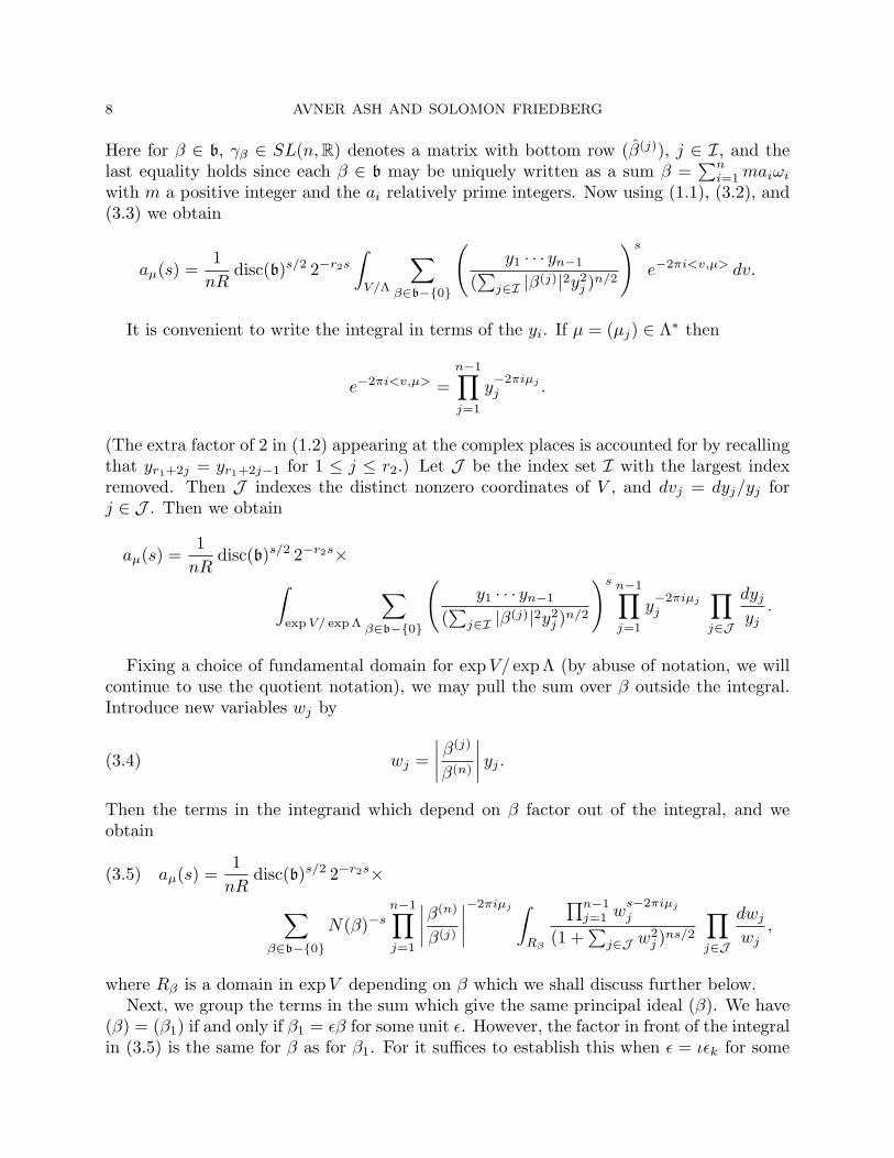
Here for β ∈ b, γβ ∈ SL(n, R) denotes a matrix with bottom row (β(j)), j ∈ I, and thelast equality holds since each β ∈ b may be uniquely written as a sum β =
∑ni=1 maiωi
with m a positive integer and the ai relatively prime integers. Now using (1.1), (3.2), and(3.3) we obtain
aµ(s) =1
nRdisc(b)s/2 2−r2s
∫V/Λ
∑β∈b−{0}
(y1 · · · yn−1
(∑
j∈I |β(j)|2y2j )n/2
)s
e−2πi<v,µ> dv.
It is convenient to write the integral in terms of the yi. If µ = (µj) ∈ Λ∗ then
e−2πi<v,µ> =n−1∏j=1
y−2πiµj
j .
(The extra factor of 2 in (1.2) appearing at the complex places is accounted for by recallingthat yr1+2j = yr1+2j−1 for 1 ≤ j ≤ r2.) Let J be the index set I with the largest indexremoved. Then J indexes the distinct nonzero coordinates of V , and dvj = dyj/yj forj ∈ J . Then we obtain
aµ(s) =1
nRdisc(b)s/2 2−r2s×∫
exp V/ exp Λ
∑β∈b−{0}
(y1 · · · yn−1
(∑
j∈I |β(j)|2y2j )n/2
)s n−1∏j=1
y−2πiµj
j
∏j∈J
dyj
yj.
Fixing a choice of fundamental domain for expV/ expΛ (by abuse of notation, we willcontinue to use the quotient notation), we may pull the sum over β outside the integral.Introduce new variables wj by
(3.4) wj =∣∣∣∣ β(j)
β(n)
∣∣∣∣ yj .
Then the terms in the integrand which depend on β factor out of the integral, and weobtain
(3.5) aµ(s) =1
nRdisc(b)s/2 2−r2s×
∑β∈b−{0}
N(β)−sn−1∏j=1
∣∣∣∣β(n)
β(j)
∣∣∣∣−2πiµj ∫Rβ
∏n−1j=1 w
s−2πiµj
j
(1 +∑
j∈J w2j )ns/2
∏j∈J
dwj
wj,
where Rβ is a domain in expV depending on β which we shall discuss further below.Next, we group the terms in the sum which give the same principal ideal (β). We have
(β) = (β1) if and only if β1 = εβ for some unit ε. However, the factor in front of the integralin (3.5) is the same for β as for β1. For it suffices to establish this when ε = ιεk for some
HECKE L-FUNCTIONS, EISENSTEIN SERIES, AND TOTALLY POSITIVE INTEGERS 9
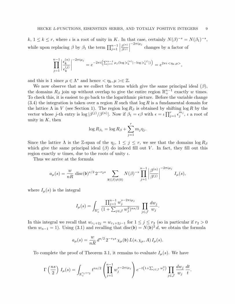
k, 1 ≤ k ≤ r, where ι is a root of unity in K. In that case, certainly N(β)−s = N(β1)−s,
while upon replacing β by β1 the term∏n−1
j=1
∣∣∣β(n)
β(j)
∣∣∣−2πiµj
changes by a factor of
n−1∏j=1
∣∣∣∣ε(n)k
ε(j)k
∣∣∣∣−2πiµj
= e−2πi
“Pn−1j=1 µj(log |ε(n)
k |−log |ε(j)k |)
”= e2πi <ηk,µ>,
and this is 1 since µ ∈ Λ∗ and hence < ηk, µ >∈ Z.We now observe that as we collect the terms which give the same principal ideal (β),
the domains Rβ join up without overlap to give the entire region Rn−1+ exactly w times.
To check this, it is easiest to go back to the logarithmic picture. Before the variable change(3.4) the integration is taken over a region R such that log R is a fundamental domain forthe lattice Λ in V (see Section 1). The region log Rβ is obtained by shifting log R by thevector whose j-th entry is log |β(j)/β(n)|. Now if β1 = εβ with ε = ι
∏rj=1 ε
mj
j , ι a root ofunity in K, then
log Rβ1 = log Rβ +r∑
j=1
mjηj .
Since the lattice Λ is the Z-span of the ηj , 1 ≤ j ≤ r, we see that the domains log Rβ
which give the same principal ideal (β) do indeed fill out V . In fact, they fill out thisregion exactly w times, due to the roots of unity ι.
Thus we arrive at the formula
aµ(s) =w
nRdisc(b)s/2 2−r2s
∑b|(β) 6=(0)
N(β)−sn−1∏j=1
∣∣∣∣β(n)
β(j)
∣∣∣∣−2πiµj
Iµ(s),
where Iµ(s) is the integral
Iµ(s) =∫
Rr+
∏n−1j=1 w
s−2πiµj
j
(1 +∑
j∈J w2j )ns/2
∏j∈J
dwj
wj.
In this integral we recall that wr1+2j = wr1+2j−1 for 1 ≤ j ≤ r2 (so in particular if r2 > 0then wn−1 = 1). Using (3.1) and recalling that disc(b) = N(b)2 d, we obtain the formula
aµ(s) =w
nRds/2 2−r2s χµ(b)L(s, χµ, A) Iµ(s).
To complete the proof of Theorem 3.1, it remains to evaluate Iµ(s). We have
Γ(ns
2
)Iµ(s) =
∫Rr1+r2
+
tns/2
n−1∏j=1
ws−2πiµj
j
e−t(1+Pj∈J w2
j)∏j∈J
dwj
wj
dt
t.

10 AVNER ASH AND SOLOMON FRIEDBERG
Changing variables wj 7→ (wj/t)1/2, j ∈ J , gives
Γ(ns
2
)Iµ(s) = 2−r
∫Rr1+r2
+
tδ s/2+π iPn−1
j=1 µj
n−1∏j=1
ws/2−πiµj
j
e−t−P
j∈J wj∏j∈J
dwj
wj
dt
t,
where δ = 1 if r2 = 0 (i.e. K is totally real) and δ = 2 otherwise. Each integral is a Gammafunction. Thus we obtain
Γ(ns
2
)Iµ(s) = 2−rΓ
s
2+ πi
n−1∑j=1
µj
n−1∏j=1
Γ(s
2− πiµj
)if r2 = 0 and
Γ(ns
2
)Iµ(s) = 2−rΓ
s + πin−2∑j=1
µj
r1∏j=1
Γ(s
2− πiµj
) r2−1∏j=1
Γ (s− 2πiµr1+2j−1)
if r2 > 0 (recall that µn−1 = 0 in this case). This completes the proof of Theorem 3.1.
Remark: The constant term a0(s) is computed adelically for a general global field in[Wi1, Wi2].
4. Dirichlet Series Constructed From Totally Real Number Fields
Suppose from now on that the field K is totally real. In this section we introduce andanalyze the Fourier coefficients of a family of Dirichlet series constructed from K. Thesecoefficients are once again related to Hecke L-functions, and the computation is effectedusing the same methods as in Section 3 above. In the next sections we shall show howthese series may be used to get information about the growth of arithmetic quantities.(Similar Dirichlet series may be studied in the non-totally-real case, but as our applicationmakes use of the totally real condition we restrict to this case for convenience.)
Let OK denote the integers of K and U be a subgroup of the units of OK which is offinite index in the full group of units O×
K and which contains −1. Let b be a fractionalideal. Let p be a function on b such that p(αu) = p(α) for all α ∈ b, u ∈ U , and such thatfor some δ, |p(α)| = O(N(α)δ) for α ∈ b. Let k ≥ 1 be a fixed integer. Let y1, · · · , yn−1
be positive real variables, y = diag(y1, · · · , yn−1, 1), and let s be complex. For notationalconvenience let yn = (y1 · · · yn−1)−1. We introduce the series
(4.1) Φ(s, y; p, k, b) =∑
0 6=α∈b
p(α)(∑n−1i=1 |α(i)|kyk
i yk/nn + |α(n)|ky
k/nn
)s .
Here yk/nn is the positive n-th root. Since
n−1∑i=1
|α(i)|kyki yk/n
n + |α(n)|kyk/nn ≥ c(y) N(α)k/n
HECKE L-FUNCTIONS, EISENSTEIN SERIES, AND TOTALLY POSITIVE INTEGERS 11
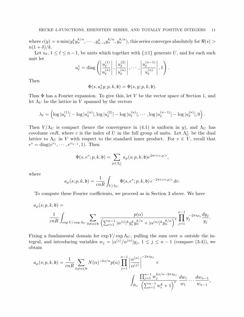
where c(y) = n min(yk1y
k/nn , · · · , yk
n−1yk/nn , y
k/nn ), this series converges absolutely for <(s) >
n(1 + δ)/k.Let u`, 1 ≤ ` ≤ n− 1, be units which together with {±1} generate U , and for each such
unit let
u∗` = diag
(∣∣∣∣∣u(1)`
u(n)`
∣∣∣∣∣ ,∣∣∣∣∣u(2)
`
u(n)`
∣∣∣∣∣ , · · · ,
∣∣∣∣∣u(n−1)`
u(n)`
∣∣∣∣∣ , 1)
.
ThenΦ(s, u∗`y; p, k, b) = Φ(s, y; p, k, b).
Thus Φ has a Fourier expansion. To give this, let V be the vector space of Section 1, andlet ΛU be the lattice in V spanned by the vectors
λ` =(log |u(1)
` | − log |u(n)` |, log |u(2)
` | − log |u(n)` |, · · · , log |u(n−1)
` | − log |u(n)` |, 0
).
Then V/ΛU is compact (hence the convergence in (4.1) is uniform in y), and ΛU hascovolume cnR, where c is the index of U in the full group of units. Let Λ∗U be the duallattice to ΛU in V with respect to the standard inner product. For v ∈ V , recall thatev = diag(ev1 , · · · , evn−1 , 1). Then
Φ(s, ev; p, k, b) =∑
µ∈Λ∗U
aµ(s; p, k, b)e2πi<v,µ>,
whereaµ(s; p, k, b) =
1cnR
∫V/ΛU
Φ(s, ev; p, k, b) e−2πi<v,µ> dv.
To compute these Fourier coefficients, we proceed as in Section 3 above. We have
aµ(s; p, k, b) =
1cnR
∫exp V/ exp ΛU
∑0 6=α∈b
p(α)(∑n−1i=1 |α(i)|kyk
i yk/nn + |α(n)|ky
k/nn
)s
n−1∏j=1
y−2πiµj
j
dyj
yj.
Fixing a fundamental domain for expV/ expΛU , pulling the sum over α outside the in-tegral, and introducing variables wj = |α(j)/α(n)|yj , 1 ≤ j ≤ n − 1 (compare (3.4)), weobtain
aµ(s; p, k, b) =1
cnR
∑0 6=α∈b
N(α)−ks/np(α)n−1∏j=1
∣∣∣∣α(n)
α(j)
∣∣∣∣−2πiµj
×
∫Rα
∏n−1j=1 w
ks/n−2πiµj
j(∑n−1i=1 wk
i + 1)s
dw1
w1· · · dwn−1
wn−1,

12 AVNER ASH AND SOLOMON FRIEDBERG
where Rα is a domain in expV depending on α.Call two nonzero field elements associate modulo U if their quotient is in U . Denote
this equivalence relation ∼. In this sum, we may group the terms corresponding to α thatare associate modulo U . Indeed, the term in front is unchanged if we replace α by αu foru ∈ U . This is verified as in Section 3. Collecting terms, the domains Rα for α which areassociate modulo U join up without overlap to give the entire region Rn−1
+ exactly twice.We arrive at the formula
aµ(s; p, k, b) =2
cnR
∑0 6=α∈b/∼
N(α)−ks/np(α)n−1∏j=1
∣∣∣∣α(n)
α(j)
∣∣∣∣−2πiµj
Iµ(s; k)
where
Iµ(s; k) =∫
Rn−1+
∏n−1j=1 w
ks/n−2πiµj
j(∑n−1i=1 wk
i + 1)s
dw1
w1· · · dwn−1
wn−1.
(Note that the integral Iµ(s) of Section 3 arises when k = 2: Iµ(s) = Iµ(ns/2; 2).)The integral Iµ(s; k) is evaluated similarly to Section 3: multiply by Γ(s) to introduce
an additional integration in a variable t and then change variables wj 7→ (wj/t)1/k. Thisgives
Γ(s) Iµ(s; k) = k−(n−1)Γ
s
n+
2πi
k
n−1∑j=1
µj
n−1∏j=1
Γ(
s
n− 2πiµj
k
).
Suppose now that p(αu) = κ(u) p(α) for all α ∈ b and u ∈ O×K , where κ is a character
of O×K/U . Then aµ(s; p, k, b) = 0 unless
(4.2) κ(u)n−1∏j=1
∣∣∣∣u(n)
u(j)
∣∣∣∣−2πiµj
= 1
for all u ∈ O×K , and in this case we have
aµ(s; p, k, b) =2
nR
∑b|(α) 6=0
N(α)−ks/np(α)n−1∏j=1
∣∣∣∣α(n)
α(j)
∣∣∣∣−2πiµj
Iµ(s; k),
where the sum is over nonzero principal integral ideals (α) divisible by b. For p a com-bination of signs and powers, the sum over (α) may be expressed in terms of the partialHecke L-function associated to the integral ideal class of b−1 in the wide ideal class group;compare (3.1).
In particular, let us analyze the functions we shall use for our estimates of integers ofgiven trace. For each i, 1 ≤ i ≤ n, choose ei = 0 or 1, and let v(α) =
∏ni=1 sgn(α(i))ei .

HECKE L-FUNCTIONS, EISENSTEIN SERIES, AND TOTALLY POSITIVE INTEGERS 13
(As the vector space V does not enter further, we change p to v to emphasize the analogyto Hecke [He].) For such a v, we consider the sum Φ(s,1; v, 1, b) where 1 = (1, . . . , 1), soall yi = 1. Denote this sum Ψ(s, v, b), that is,
(4.3) Ψ(s, v, b) =∑
0 6=α∈b
v(α)((|α(1)|+ · · ·+ |α(n)|)s
.
This sum converges for <(s) > n. This function is 0 unless v(α) = v(−α). Let U denote thesubgroup of units which are either totally positive or totally negative. Let v0 correspondto ei = 0 for all i. Then we shall show
Proposition 4.1. Each function Ψ(s, v, b) has meromorphic continuation to the right halfplane <(s) > 0. The functions Ψ(s, v, b) are holomorphic in this right half plane for v 6= v0,while Ψ(s, v0, b) has a simple pole at s = n of residue
2n
(n− 1)! disc(b)1/2.
Proof. By the computation above, for <(s) > n we have
(4.4) Ψ(s, v, b) =∑
µ∈Λ∗U
aµ(s; v, 1, b).
In this sum only µ satisfying (4.2) (with κ = v) contribute. For such µ, let
λµ,v(α) =n−1∏j=1
∣∣∣∣α(n)
α(j)
∣∣∣∣−2πiµj
v(α).
Extend λµ,v to a Hecke character as in Section 3. Let L(s, λµ,v, A) be the partial HeckeL-function associated to the integral ideal class A of b−1 , and let
Γ(s, λµ,v) = (π−nd)s/2Γ
s
2+
en
2+ πi
n−1∑j=1
µj
n−1∏j=1
Γ(s
2+
ej
2− πiµj
)be the standard Gamma factor attached to L(s, λµ,v). Let
L∗(s, λµ,v, A) = Γ(s, λµ,v) L(s, λµ,v, A)
be the partial L-function for the integral ideal class A with Gamma factors included. Thenwe may express the coefficients in (4.4) in terms of these Hecke L-functions. Indeed, wesee, as in (3.1), that
(4.5) aµ(s; v, 1, b) =2
nRN(b)−s/nλµ,v(b)L
(sn , λµ,v, A
)Iµ(s; 1)

14 AVNER ASH AND SOLOMON FRIEDBERG
with
(4.6) Iµ(s; 1) = Γ(s)−1Γ
s
n+ 2πi
n−1∑j=1
µj
n−1∏j=1
Γ( s
n− 2πiµj
).
At this point we could analyze the convergence of the sum (4.4) by the use of Stirling’sformula, Phragmen-Lindelof estimates, and geometric arguments. In fact, we shall do soin Section 8 below. However, to prove the Proposition a simpler argument suffices, whichwe now give. Using the duplication formula
Γ(z) = Γ(z/2) Γ((z + 1)/2) 2z−1 π−1/2
we find thataµ(s; v, 1, b) =
2nR
N(b)−s/nλµ,v(b)L∗( sn , λµ,v, A) Jµ(s)
where
Jµ(s) = π(s−n)/2 2s−n d−s/2n×
Γ(s)−1Γ
s
2n+
1− en
2+ πi
n−1∑j=1
µj
n−1∏j=1
Γ(
s
2n+
1− ej
2− πiµj
).
Since each function L∗ may be represented as the Mellin transform of a suitable thetafunction, it is easy to see that the functions L∗( s
n , λµ,v, A) are bounded on vertical stripsindependently of µ (except for v = v0, µ = 0, where we must stay away from the pole ats = n). By Stirling’s formula, one sees that the expansion (4.4) converges uniformly for sin a compact set (in fact, lying in a vertical strip of bounded width) provided one avoidsthe lines of poles coming from the Gamma factors. In particular, Ψ(s, v, b) continues tothe right half plane <(s) > 0, as claimed. Moreover, the Gamma factors have no poles for<(s) > 0, so the functions Ψ(s, v, b) are regular in the right half plane except for Ψ(s, v0, b).
To analyze the residue at s = n of Ψ(s, v0, b), observe that all the terms in the Fourierexpansion of Φ(s, y; 1, 1, b) are holomorphic in the right half plane except for a0(s; 1, 1, b),which is expressed in terms of a partial Dedekind zeta function evaluated at s/n. Thisfunction has its only pole in the right half plane at s = n. Since I0(n; 1) = 1/Γ(n), theresidue is given by
Ress=n Ψ(s, v0, b) = Ress=n a0(s; 1, 1, b) =2n
(n− 1)! disc(b)1/2.
This completes the proof of the Proposition.
Remark: This proof closely follows Hecke [He] who studied the case n = 2. However,the case n > 2 is different from this case in a fundamental way. To explain this, let us

HECKE L-FUNCTIONS, EISENSTEIN SERIES, AND TOTALLY POSITIVE INTEGERS 15
study the series given by (4.4) in the half plane <(s) ≤ 0. From (4.5), (4.6), it follows thateach function aµ(s, v, 1, b) has possible poles at
s = −2nk + n(ej − 1) + 2πinµj , 1 ≤ j ≤ n− 1
and at
s = −2nk + n(en − 1)− 2πinn−1∑j=1
µj
for each k = 0, 1, 2, . . . . When we sum over µ ∈ Λ∗U , for n > 2 these locations are denseon the vertical lines <(s) = −2nk + n(ej − 1), 1 ≤ j ≤ n, k = 0, 1, 2, . . . , as we showmomentarily. Thus it does not seem possible to use this to continue to the functionsΨ(s, v, b) to all complex s.
To see that if n > 2 the poles are dense, suppose without loss of generality that theunits u1, . . . , un−1 are totally positive. They are also multiplicatively independent. Definethe (n − 1) × (n − 1) matrix Λ by Λi,j = log u
(i)j − log u
(n)j , and let M = Λ−1. Then the
entries of M are the coordinates of the µ’s which make up a Z-bases of the lattice Λ∗U . Toprove that the poles are dense on any vertical line with real part as indicated, it suffices toshow that at least two of these entries are linearly independent over Q, since if r1, r2 ∈ Rwith r1/r2 6∈ Q, then {mr1 + nr2 | m,n ∈ Z} is dense in R.
Suppose not. Then M = θR where θ ∈ R and R ∈ GL(n, Q). Let E be a matrix inGL(n, Q) such that premultiplication by E adds all the other rows to the last row. Since foreach j,
∑ni=1 log u
(i)j = 0, we see that EΛ has bottom row −n(log u
(n)1 , . . . , log u
(n)n−1). Also,
since (EΛ)(RE−1) = θ−1I, we see that there is a nonzero integral vector (c1, . . . , cn−1)whose dot product with the bottom row of (EΛ) is 0. (A suitable integral multiple of anyof the columns of RE−1 except the last will do.) Then we have
∑i ci log u
(n)i = 0. But
this implies that∏
i ucii = 1 which contradicts the multiplicative independence of the units
ui. Hence for n > 2 the poles are dense.
5. A Geometric Computation
Let a denote a fractional ideal in the ring of integers of K. Let αj ∈ a, j = 1, . . . , n bea Z-basis of a. The absolute trace from K to Q defines a linear map Tr from a to the freeabelian subgroup of Q generated by k > 0. (The parameter k here is not the same as inSection 4 above.) Denote the set of elements of a with trace 0 by a0. Then we may assumethat Tr(α1) = k and that αj ∈ a, j = 2, . . . , n is a Z-basis of a0.
Let a denote a positive integral multiple of k. In this section, we compute the ratio ra
of two volumes: (1) the volume of the simplex Sa of totally positive elements of a0⊗R+β,where β ∈ a is a fixed element with trace a, and (2) the volume of the fundamental cell ofthe lattice a0 in a0 ⊗ R. Since ra is a ratio, it is independent of the normalization of thevolume on a0 ⊗ R.
Our result is:
16 AVNER ASH AND SOLOMON FRIEDBERG
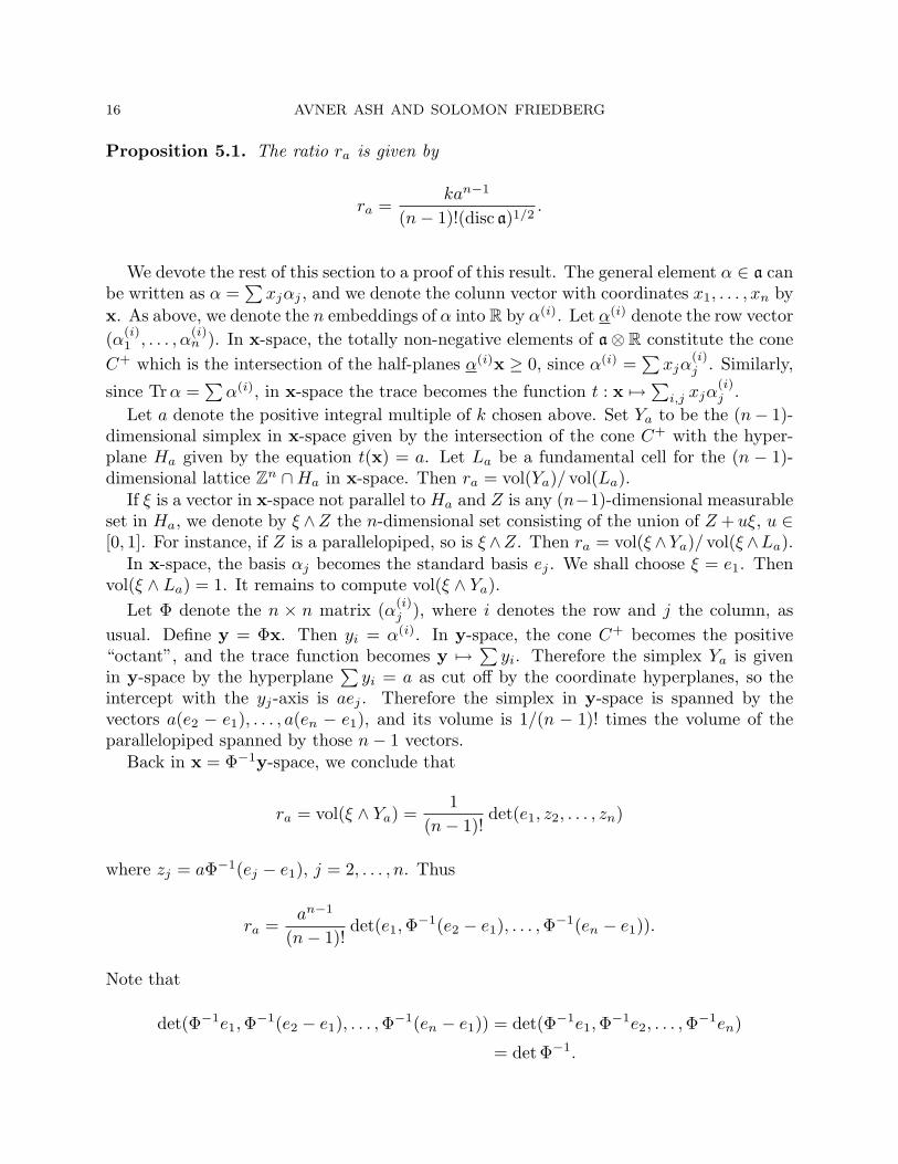
Proposition 5.1. The ratio ra is given by
ra =kan−1
(n− 1)!(disc a)1/2.
We devote the rest of this section to a proof of this result. The general element α ∈ a canbe written as α =
∑xjαj , and we denote the colunn vector with coordinates x1, . . . , xn by
x. As above, we denote the n embeddings of α into R by α(i). Let α(i) denote the row vector(α(i)
1 , . . . , α(i)n ). In x-space, the totally non-negative elements of a⊗R constitute the cone
C+ which is the intersection of the half-planes α(i)x ≥ 0, since α(i) =∑
xjα(i)j . Similarly,
since Trα =∑
α(i), in x-space the trace becomes the function t : x 7→∑
i,j xjα(i)j .
Let a denote the positive integral multiple of k chosen above. Set Ya to be the (n− 1)-dimensional simplex in x-space given by the intersection of the cone C+ with the hyper-plane Ha given by the equation t(x) = a. Let La be a fundamental cell for the (n − 1)-dimensional lattice Zn ∩Ha in x-space. Then ra = vol(Ya)/ vol(La).
If ξ is a vector in x-space not parallel to Ha and Z is any (n−1)-dimensional measurableset in Ha, we denote by ξ ∧Z the n-dimensional set consisting of the union of Z + uξ, u ∈[0, 1]. For instance, if Z is a parallelopiped, so is ξ∧Z. Then ra = vol(ξ∧Ya)/ vol(ξ∧La).
In x-space, the basis αj becomes the standard basis ej . We shall choose ξ = e1. Thenvol(ξ ∧ La) = 1. It remains to compute vol(ξ ∧ Ya).
Let Φ denote the n × n matrix (α(i)j ), where i denotes the row and j the column, as
usual. Define y = Φx. Then yi = α(i). In y-space, the cone C+ becomes the positive“octant”, and the trace function becomes y 7→
∑yi. Therefore the simplex Ya is given
in y-space by the hyperplane∑
yi = a as cut off by the coordinate hyperplanes, so theintercept with the yj-axis is aej . Therefore the simplex in y-space is spanned by thevectors a(e2 − e1), . . . , a(en − e1), and its volume is 1/(n − 1)! times the volume of theparallelopiped spanned by those n− 1 vectors.
Back in x = Φ−1y-space, we conclude that
ra = vol(ξ ∧ Ya) =1
(n− 1)!det(e1, z2, . . . , zn)
where zj = aΦ−1(ej − e1), j = 2, . . . , n. Thus
ra =an−1
(n− 1)!det(e1,Φ−1(e2 − e1), . . . ,Φ−1(en − e1)).
Note that
det(Φ−1e1,Φ−1(e2 − e1), . . . ,Φ−1(en − e1)) = det(Φ−1e1,Φ−1e2, . . . ,Φ−1en)
= det Φ−1.

HECKE L-FUNCTIONS, EISENSTEIN SERIES, AND TOTALLY POSITIVE INTEGERS 17
It follows that
det(e1,Φ−1(e2 − e1), . . . ,Φ−1(en − e1))− detΦ−1
= det(e1 − Φ−1e1,Φ−1(e2 − e1), . . . ,Φ−1(en − e1))
= det Φ−1 · det(Φe1 − e1, e2 − e1, . . . , en − e1).
The first column of Φ is (α(i)1 ), so the last determinant mentioned equals
det
α
(1)1 − 1 −1 −1 . . . −1α
(2)1 1 0 . . . 0
α(3)1 0 1 . . . 0...
......
......
α(n)1 0 0 . . . 1
which equals Tr(α1) − 1 = k − 1. Therefore, using the fact that det Φ = (disc a)1/2, weobtain the evaluation of ra stated in the Proposition.
6. Comparing the Residues
As in the preceding section, let a denote a fractional ideal in the ring of integers of K,and let Tr(a) be generated by k > 0. If a is a positive integral multiple of k, let Na denotethe number of totally positive elements of a with trace a. One may obtain an estimate ofNa by standard methods for counting lattice points in homogeneously expanding domains.Indeed, from Chapter VI, Theorem 2 of Lang [Lang], we find that Na is approximated byexactly the volume ratio ra, and from that result we conclude that there exists a constantd such that
(6.1) |Na − ra| ≤ d|a|n−2
for all such a.Our goal here is to study the difference Ea = Na − ra between Na and its estimate as
a volume. If a is not a positive multiple of k, we set Ea = 0. To do so, we study theDirichlet series
ϕ(s) =∑a>0
Ea
as.
By (6.1), this series converges absolutely for <(s) > n− 1. Writing a = mk, (6.1) gives atrivial bound: for s > n− 1 real,
|ϕ(s)| ≤∑m>0
dkn−2mn−2
ksms= dkn−2−sζ(s− n + 2).
The right hand side has a pole at s = n − 1. However, we should expect considerablecancelation in the series for ϕ(s). In fact, we shall now show

18 AVNER ASH AND SOLOMON FRIEDBERG
Proposition 6.1. The function ϕ(s) is holomorphic for <(s) > 0.
Proof. For i = 1, . . . n, choose ei = 0 or 1. Then for α ∈ a set v(α) =∏n
i=1(sgn(α(i))ei).There are 2n possible v’s. Recall that Ψ(s, v, a) is given by (4.3). Summing over all the vwe get ∑
v
Ψ(s, v, a) = 2n∑
0�α∈a
1Tr(α)s
= 2n∑a>0
Na
as.
Substituting ra + Ea for Na, and setting a = mk as above, we obtain
(6.2)∑
v
Ψ(s, v, a) = 2n kn−s
(n− 1)!(disc a)1/2ζ(s− n + 1) + 2n
∑a>0
Ea
as.
On the other hand, by Proposition 4.1,∑
v Ψ(s, v, a) is holomorphic for <(s) > 0 exceptfor a simple pole at s = n with residue
2n
(n− 1)!(disc a)1/2.
Since the same is true of
2n kn−s
(n− 1)!(disc a)1/2ζ(s− n + 1),
we obtain that the Dirichlet series
ϕ(s) =∑a>0
Ea
as
is holomorphic for <(s) > 0 as claimed.
7. Some Geometric Preliminaries
Our next task is to analyze the growth of ϕ(s) in vertical strips. To do this, we willcombine Stirling’s formula with the Fourier expansion (4.4). We require some informationconcerning the number of points in the intersection of a lattice with a certain family ofcompact polyhedra. We address this now.
Let us fix a Euclidean metric on Rn for this whole section. For η ∈ Rn and r > 0, letBr(η) denote the closed ball around η of radius r.
Lemma 7.1. Let Λ ⊂ Rn be a lattice and S ⊂ Rn be a compact set. Fix a fundamentalcell Π0 of Λ. Let ρ be the diameter of Π0 and d be the diameter of S. Let γn be the volumeof the unit sphere in Rn. Then
card(Λ ∩ S) ≤ γn(d + ρ)n/ det(Λ).
Proof. If card(Λ ∩ S) = 0, there is nothing to prove. If not, fix λ0 ∈ Λ ∩ S. Claim:for any λ ∈ Λ ∩ S, Bρ(λ) ⊂ Bd+ρ(λ0). Indeed, dist(λ, λ0) ≤ d, and for any x ∈ Bρ(λ),dist(λ, x) ≤ ρ. Therefore, dist(λ0, x) ≤ d + ρ.
It follows that ⋃λ∈Λ∩S
(λ + Π0) ⊂ Bd+ρ(λ0).
The volume of the union is (detΛ) card(Λ∩S) and the volume of the ball is γn(d+ρ)n.
HECKE L-FUNCTIONS, EISENSTEIN SERIES, AND TOTALLY POSITIVE INTEGERS 19
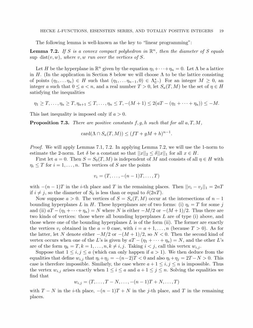
The following lemma is well-known as the key to “linear programming”:
Lemma 7.2. If S is a convex compact polyhedron in Rn, then the diameter of S equalssup dist(v, w), where v, w run over the vertices of S.
Let H be the hyperplane in Rn given by the equation η1+· · ·+ηn = 0. Let Λ be a latticein H. (In the application in Section 8 below we will choose Λ to be the lattice consistingof points (η1, . . . ηn) ∈ H such that (η1, . . . ηn−1, 0) ∈ Λ∗U .) For an integer M ≥ 0, aninteger a such that 0 ≤ a < n, and a real number T > 0, let Sa(T,M) be the set of η ∈ Hsatisfying the inequalities
η1 ≥ T, . . . , ηa ≥ T, ηa+1 ≤ T, . . . , ηn ≤ T,−(M + 1) ≤ 2(aT − (η1 + · · ·+ ηa)) ≤ −M.
This last inequality is imposed only if a > 0.
Proposition 7.3. There are positive constants f, g, h such that for all a, T,M ,
card(Λ ∩ Sa(T,M)) ≤ (fT + gM + h)n−1.
Proof. We will apply Lemmas 7.1, 7.2. In applying Lemma 7.2, we will use the 1-norm toestimate the 2-norm. Let δ be a constant so that ||x||2 ≤ δ||x||1 for all x ∈ H.
First let a = 0. Then S = S0(T,M) is independent of M and consists of all η ∈ H withηi ≤ T for i = 1, . . . , n. The vertices of S are the points
vi = (T, . . . ,−(n− 1)T, . . . , T )
with −(n − 1)T in the i-th place and T in the remaining places. Then ||vi − vj ||1 = 2nTif i 6= j, so the diameter of S0 is less than or equal to δ(2nT ).
Now suppose a > 0. The vertices of S = Sa(T,M) occur at the intersections of n − 1bounding hyperplanes L in H. These hyperplanes are of two forms: (i) ηi = T for some jand (ii) aT − (η1 + · · ·+ ηa) = N where N is either −M/2 or −(M + 1)/2. Thus there aretwo kinds of vertices: those where all bounding hyperplanes L are of type (i) above, andthose where one of the bounding hyperplanes L is of the form (ii). The former are exactlythe vertices vi obtained in the a = 0 case, with i = a + 1, . . . , n (because T > 0). As forthe latter, let N denote either −M/2 or −(M + 1)/2, so N < 0. Then the second kind ofvertex occurs when one of the L’s is given by aT − (η1 + · · ·+ ηa) = N , and the other L’sare of the form ηk = T, k = 1, . . . , n, k 6= i, j. Taking i < j, call this vertex wi,j .
Suppose that 1 ≤ i, j ≤ a (which can only happen if a > 1). We then deduce from theequalities that define wi,j that ηi+ηj = −(n−2)T < 0 and also ηi+ηj = 2T−N > 0. Thiscase is therefore impossible. Similarly, the case where a + 1 ≤ i, j ≤ n is impossible. Thusthe vertex wi,j arises exactly when 1 ≤ i ≤ a and a + 1 ≤ j ≤ n. Solving the equalities wefind that
wi,j = (T, . . . , T −N, . . . ,−(n− 1)T + N, . . . , T )
with T − N in the i-th place, −(n − 1)T + N in the j-th place, and T in the remainingplaces.

20 AVNER ASH AND SOLOMON FRIEDBERG
We estimate the diameter by computing the 1-norm of the difference of pairs of vertices.We have ||vk − wi,j ||1 = 2nT − 2N if k 6= j and −2N if k = j. Similarly, there are fourpossibilities for ||wi,j − wk.m||1; these give (0 or − 2N) + (0 or 2nT − 2N). Thus thediameter of S is less than or equal to δ(2nT + 2M + 2) in all cases, including where a = 0.
We now apply Lemma 7.1. If we let ρ denote the diameter of our fundamental cell inΛ, then
card(Λ ∩ S) ≤ γn(δ(2nT + 2M + 2) + ρ)n−1/ det Λ.
This proves the Proposition.
8. The Distribution of Totally Positive Integers of Given Trace
In this section we further study the function ϕ and use this to obtain our main result.We have
Proposition 8.1. Given ε, δ > 0, then
ϕ(s) = O(|t|n−1/2−σ/2+ε)
as t →∞ uniformly for s = σ + it with δ ≤ σ ≤ n.
Proof. An estimate of this form for ζ(s − n + 1) follows immediately from convexity. Inview of (6.2), it suffices to establish such an estimate for each function Ψ(s, v, a). Denotethe Fourier coefficients of such a function aµ(s). For convenience, let µn = −
∑n−1j=1 µj .
We use the expressions (4.5), (4.6). By the convexity bound for the L-function obtainedfrom Phragmen-Lindelof we have
L( sn , λµ,v, A) �
n∏j=1
∣∣ tn − 2πµj
∣∣(1−σ/n)/2+ε
as |t| → ∞, uniformly in the strip. Combining with Stirling’s formula, one sees that
aµ(s) � |t|1/2−σeπ|t|/2n∏
j=1
∣∣ tn − 2πµj
∣∣(σ/2n)+εe−
π2 |
tn−2πµj |.
Let
F (s, µ) =n∏
j=1
∣∣ tn − 2πµj
∣∣(σ/2n)+εe−
π2 |
tn−2πµj |.
Then ∑µ∈Λ∗U
|aµ(s)| � |t| 12−σeπ2 |t|∑
µ
F (s, µ).
We must estimate this sum.
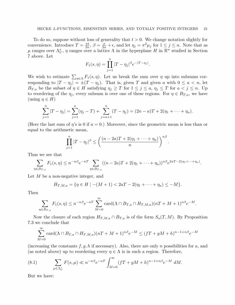
HECKE L-FUNCTIONS, EISENSTEIN SERIES, AND TOTALLY POSITIVE INTEGERS 21
To do so, suppose without loss of generality that t > 0. We change notation slightly forconvenience. Introduce T = πt
2n , β = σ2n + ε, and let ηj = π2µj for 1 ≤ j ≤ n. Note that as
µ ranges over Λ∗U , η ranges over a lattice Λ in the hyperplane H in Rn studied in Section7 above. Let
F1(s, η) =n∏
j=1
|T − ηj |βe−|T−ηj |.
We wish to estimate∑
η∈Λ F1(s, η). Let us break the sum over η up into subsums cor-responding to |T − ηj | = ±(T − ηj). That is, given T and given a with 0 ≤ a < n, letBT,a be the subset of η ∈ H satisfying ηj ≥ T for 1 ≤ j ≤ a, ηj ≤ T for a < j ≤ n. Upto reordering of the ηj , every subsum is over one of these regions. For η ∈ BT,a, we have(using η ∈ H)
n∑j=1
|T − ηj | =a∑
j=1
(ηj − T ) +n∑
j=a+1
(T − ηj) = (2n− a)T + 2(η1 + · · ·+ ηa).
(Here the last sum of η’s is 0 if a = 0.) Moreover, since the geometric mean is less than orequal to the arithmetic mean,
n∏j=1
|T − ηj |β ≤(
(n− 2a)T + 2(η1 + · · ·+ ηa)n
)nβ
.
Thus we see that∑η∈BT,a
F1(s, η) ≤ n−nβe−nT∑
η∈BT,a
((n− 2a)T + 2(η1 + · · ·+ ηa))nβe2aT−2(η1+···+ηa).
Let M be a non-negative integer, and
HT,M,a = {η ∈ H | −(M + 1) < 2aT − 2(η1 + · · ·+ ηa) ≤ −M}.
Then ∑η∈BT,a
F1(s, η) ≤ n−nβe−nT∞∑
M=0
card(Λ ∩BT,a ∩HT,M,a)(nT + M + 1)nβe−M .
Now the closure of each region HT,M,a ∩BT,a is of the form Sa(T,M). By Proposition7.3 we conclude that
∞∑M=0
card(Λ ∩BT,a ∩HT,M,a)(nT + M + 1)nβe−M ≤ (fT + gM + h)n−1+nβe−M
(increasing the constants f, g, h if necessary). Also, there are only n possibilities for a, and(as noted above) up to reordering every η ∈ Λ is in such a region. Therefore,
(8.1)∑
µ∈Λ∗U
F (s, µ) � n−nβe−nT
∫ ∞
M=0
(fT + gM + h)n−1+nβe−M dM.
But we have:
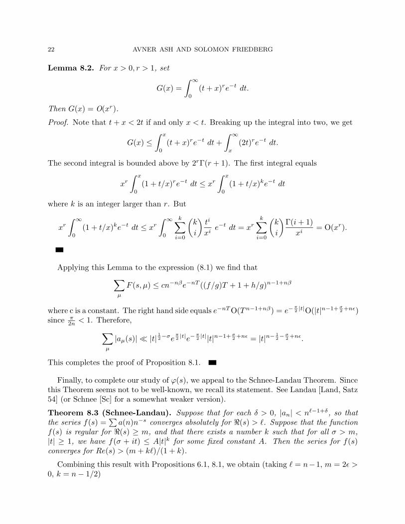
22 AVNER ASH AND SOLOMON FRIEDBERG
Lemma 8.2. For x > 0, r > 1, set
G(x) =∫ ∞
0
(t + x)re−t dt.
Then G(x) = O(xr).
Proof. Note that t + x < 2t if and only x < t. Breaking up the integral into two, we get
G(x) ≤∫ x
0
(t + x)re−t dt +∫ ∞
x
(2t)re−t dt.
The second integral is bounded above by 2rΓ(r + 1). The first integral equals
xr
∫ x
0
(1 + t/x)re−t dt ≤ xr
∫ x
0
(1 + t/x)ke−t dt
where k is an integer larger than r. But
xr
∫ ∞
0
(1 + t/x)ke−t dt ≤ xr
∫ ∞
0
k∑i=0
(k
i
)ti
xie−t dt = xr
k∑i=0
(k
i
)Γ(i + 1)
xi= O(xr).
Applying this Lemma to the expression (8.1) we find that∑µ
F (s, µ) ≤ cn−nβe−nT ((f/g)T + 1 + h/g)n−1+nβ
where c is a constant. The right hand side equals e−nT O(Tn−1+nβ) = e−π2 |t|O(|t|n−1+ σ
2 +nε)since π
2n < 1. Therefore,∑µ
|aµ(s)| � |t| 12−σeπ2 |t|e−
π2 |t||t|n−1+ σ
2 +nε = |t|n− 12−
σ2 +nε.
This completes the proof of Proposition 8.1.
Finally, to complete our study of ϕ(s), we appeal to the Schnee-Landau Theorem. Sincethis Theorem seems not to be well-known, we recall its statement. See Landau [Land, Satz54] (or Schnee [Sc] for a somewhat weaker version).
Theorem 8.3 (Schnee-Landau). Suppose that for each δ > 0, |an| < n`−1+δ, so thatthe series f(s) =
∑a(n)n−s converges absolutely for <(s) > `. Suppose that the function
f(s) is regular for <(s) ≥ m, and that there exists a number k such that for all σ > m,|t| ≥ 1, we have f(σ + it) ≤ A|t|k for some fixed constant A. Then the series for f(s)converges for Re(s) > (m + k`)/(1 + k).
Combining this result with Propositions 6.1, 8.1, we obtain (taking ` = n−1, m = 2ε >0, k = n− 1/2)
HECKE L-FUNCTIONS, EISENSTEIN SERIES, AND TOTALLY POSITIVE INTEGERS 23
Theorem 8.4. The series∑
Eaa−s converges for <(s) > n− 1− (2n− 2)/(2n + 1).
Then, by partial summation, we get our result concerning the distribution of the totallypositive elements of the fractional ideal a of trace a.
Main Theorem. For ε > 0, ∑a<X
Ea = O(Xn−1− 2n−2
2n+1 +ε)
.
References
[B-G] D. Bump and D. Goldfeld, A Kronecker limit formula for cubic fields, Modular forms (Durham,
1983), Ellis Horwood, Horwood, Chichester, 1984, pp. 43–49.[C-G] G. Chinta and D. Goldfeld, Grossencharakter L-functions of real quadratic fields twisted by modular
symbols, Invent. Math. 144 (2001), 435–449.
[D-I] W. Duke and I. Immamoglu, Lattice points in cones and Dirichlet series (preprint).[Ef] I. Efrat, On a GL(3) analog of |η(z)|, J. Number Theory 40 (1992), 174–186.
[He] E. Hecke, Uber analytische Funktionen und die Verteilung von Zahlen mod.Eins, Abh. Math.
Seminar Hamburg 1 (1921), 54–76; in Mathematische Werke, Vandenhoeck & Ruprecht, Gottingen,1983, pp. 313–335.
[Land] Landau, Handbuch der Lehre von der Verteilung der Primzahlen. 2 Bnde., 2d ed. With an appendixby Paul T. Bateman, Chelsea Publishing Co., New York, 1953.
[Lang] S. Lang, Algebraic Number Theory, Addison-Wesley Publishing Company, Reading, Massachusetts,
1970.[Sc] W. Schnee, Uber den Zusammenghang zwischen den Summabilitatseigenschaften Dirichletscher
Reihen und irhem Funkionentheoretischen Charakter, Acta Mathematica 35 (1912), 357–398.
[Si] C. L. Siegel, Advanced Analytic Number Theory, Tata Institute of Fundamental Research, Bombay,1980.
[Wi1] F. Wielonsky, Integrales toroıdales des series d’Eisenstein et fonctions zeta, C. R. Acad. Sci. Paris
299 (1984), 727–730.[Wi2] F. Wielonsky, Series d’Eisenstein, integrales toroıdales et une formule de Hecke, L’Enseignment
Mathematique 31 (1985), 93–135.