helpful comments from kevin fox, paul mccarthy, shiji zhao
TRANSCRIPT

1
Estimating substitution bias in Price Indexes: An empirical
investigation using scanner data
Lorraine Ivancic ∗
School of Economics
University of New South Wales
Sydney, Australia 2052
Email: [email protected]
Tel: +612 9385 3188
September 1st, 2005
ABSTRACT
This paper examines the issue of estimating substitution bias using scanner data. The
results show that the estimates of substitution bias are quite sensitive to both the method
of aggregation employed – over time and stores – and whether direct or chained indexes
are used. Consistent with previous evidence, chaining, particularly at high frequencies,
was found to increase the volatility of our estimates of substitution bias considerably.
Different from previous studies, results are reported for a wide range of goods. The use of
dissimilarity indexes has been recommended by the ILO (2004) to determine when it is
appropriate to chain. However, this paper finds that dissimilarity indexes may not be
sufficient to resolve the issue of when to chain.
∗ Helpful comments from Kevin Fox, Paul McCarthy, Shiji Zhao, Merry Branson and Geoff Lee are gratefully acknowledged. Support from the Australian Bureau of Statistics (ABS) has greatly facilitated this research, not least through the provision of the scanner data set. This paper is the responsibility of the author and does not reflect the views or opinions of any of the above mentioned parties.

2
1. Introduction
Whether the consumer price index (CPI) is biased, and if so, by how much, are issues
which have gained a considerable amount of international attention in recent years. This
paper examines the issue using electronicpointofsale (‘scanner’) data a rich set of
data collected from supermarkets. Scanner data provides a vast amount of information on
prices and quantities relative to what is typically used by statistical agencies in their
production of price indexes. Therefore, it allows the investigation of various aspects of
price index construction that are difficult to do with traditional data sources.
Much of the recent interest in potential bias in the CPI has stemmed from the release of
the Boskin Commission report in 1996, titled ‘Towards a more accurate measure of the
cost of living’. The aim of the report was to investigate whether the U.S. CPI was biased
and to make recommendations where appropriate. Fundamental to the findings and
recommendations made in the Boskin Commission report was the idea that the CPI
should be a measure of changes in the cost of living. This view is not held by all
statistical agencies. Therefore, the following discussion is only relevant where the cost
ofliving approach is taken.
One of the main findings of the Boskin Commission report was that current methods used
to estimate the U.S. CPI lead to upwardly biased estimates. Bias was estimated to be
between 0.8 and 1.6% per annum (Boskin, et al. 1996). The report attributed the upward
bias of the CPI to four sources: quality change bias, new goods bias, item substitution
bias and outlet substitution bias. These sources of bias are defined by Boskin, et al.
(1996) as follows:
Quality change bias: Occurs when quality improvements in products are not
accounted for (or are accounted for incorrectly);
New goods bias: Occurs when new goods are not included in the market basket
(or are included only after a long lag);
Item substitution bias: Occurs when a consumer’s ability to substitute away from
relatively expensive goods to relatively cheaper goods goes unaccounted; and

3
Outlet substitution bias: Occurs when a consumer’s ability to substitute away
from relatively expensive outlets to relatively cheaper outlets goes unaccounted.
Substitution bias contributed significantly to the overall bias in the index and was
estimated to account for just over 1/3 of the total bias. The estimation of item substitution
bias is the focus of this paper.
To attempt to account for substitution bias base period and current period price and
quantity data are needed. In the past this information has not been readily available and
therefore, issues such as how to account for substitution bias have remained unresolved.
However, the recent widespread adoption of bar code technology in retail outlets has
enabled the collection of large quantities of uptodate information on both prices paid by
consumers and quantities purchased. As a result, these data sets have made it possible to
construct indexes which have the potential to account for biases.
Conceptually, the issue of accounting for substitution bias appears to be quite easily
resolved with the availability of scanner data. However, underlying the estimates of
substitution bias are choices about the method of aggregation ie. how we aggregate over
items, outlets and time, which index number formula to use and whether or not to chain.
This paper explores whether and how choices about aggregation and the use of direct
chained indexes impact on estimates of substitution bias. Work undertaken to estimate
substitution bias with scanner data in the past has been limited by the small number of
product categories contained in the datasets used. For instance, Feenstra and Shapiro
(2001), Silver and Heravi (2001), and Reinsdorf (1999) had information on only one
product category tuna, television sets and coffee respectively, while Dalen (1997) had
information on four product categories – fats, detergent, breakfast cereal and frozen fish.
A major benefit of the data set used in this study is that it contains information on 19
product categories. This allows us to determine whether results found in other studies
hold for a larger set of products and whether the same patterns hold for different product
categories.

4
Much of the background and ideas explored in this paper are based on information
contained in the Consumer Price Index Manual: Theory and Practice (International
Labour Organisation (ILO), 2004). The aim of the manual was to ‘…develop and
document best practice guidelines on concepts and methods of price statistics and
indicators consistent with the established international standards on the subject’ (ILO
webpage 2005: http://www.ilo.org/public/english/bureau/stat/guides/cpi/iwgtor.htm ). In
1998 the ILO, ECE, IMF1, World Bank, OECD, Eurostat and UNSD took on the
responsibility of revising the manual to reflect changes which had occurred since the last
version produced in 1987. These efforts led to the 2004 version of the CPI manual.
The paper is set out as follows. Section 2 provides a brief description of the data used in
this research. A general discussion on how we define and estimate substitution bias, and
how decisions about aggregation (over prices and quantities) must be made to estimate
substitution bias is provided in section 3. Estimates of substitution bias, based on
different methods of aggregation, are presented in section 4. The impact of chaining on
estimates of substitution bias and an exploration of when chaining is appropriate is
presented in sections 5 and 6, respectively. Section 7 sums up the findings of the paper
and suggests where future research efforts in this area might be productively focused.
1. The Data
This paper uses a scanner data set collected by A.C. Neilson. The data set contains
information on four supermarket chains located in one of the major capital cites in
Australia. In total, over 100 stores are included in this data set with these stores
accounting for approximately 80% of grocery sales in this city (Jain and Abello, 2001).
The data set contains 65 weeks of data, collected between February 1997 and April 1998.
Information on 19 different supermarket item categories, such as bread and biscuits, are
included. Within each product category, information is included on a range of brands
which were found in each of the stores.
An important feature of the data is that it has been aggregated to weekly data, which
means that the data set includes information on the average price (unit value) of each

5
item sold in each store each week and the total quantity of that item sold in each store
each week. Additional information includes the product brand name, a unique 13 digit
identifier (known as the Australian Product Number (APN)) and, where relevant, the
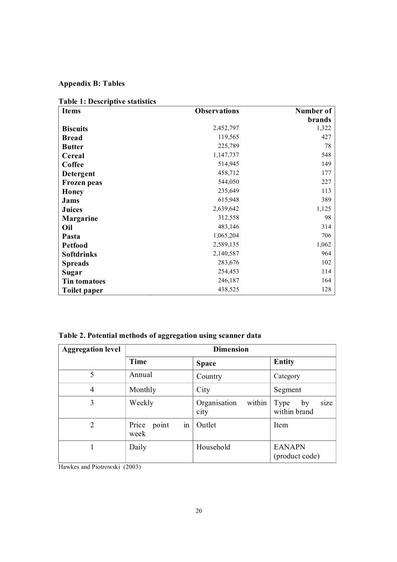
physical weight of the item. Table 1 provides some additional information on the data set.
The data set includes a large number of observations for all of the item categories over
the 65 week period. The smallest number of observations for a particular item is
approximately 120,000 for the item bread, while the largest number of observations is
just over two and a half million for the item categories juices and pet food. Within each
item category the data set contains price and quantity information on a considerable
number of brands. The highly detailed nature of the data enables us to calculate
substitution bias more accurately than what is possible with traditional data sources (eg.
surveys).
2. What is substitution bias and how do we estimate it?
The Consumer Price Index is a measure of the cost of purchasing a fixed basket of goods
and services in two different periods (Boskin et al, 1996). Theoretically the basket of
goods can be fixed to represent either base period or current period consumption. Indexes
which reflect these two different market baskets are known as Laspeyres and Paasche
indexes, respectively and are defined in equations (1) and (2). If price and quantity
relatives are negatively correlated the Laspeyres price index will be higher that the
corresponding Paasche index (ILO, 2004).
Laspeyres and Paasche indexes are defined here as:
= ∑
0 0
i
it
i i t p
p w Laspeyres (1)
1
0
−
= ∑
i it
i it t p p
w Paasche (2)
Where: Pi0 = price of item i in period 0 pit = price of item i in period t it w = good i’s share of total expenditure in period t t = 1,…,T
6
The ‘fixedbasket’ nature of the Laspeyres index does not allow for consumers to
substitute away from goods that have become relatively more expensive to goods that
have become relatively cheaper between the two periods. The inability of a price index to
capture consumer substitution is known as substitution bias. In the past CPI measurement
has typically been based on a Laspeyrestype index.
An alternative view which has become popular in recent years is that the CPI should be
used to measure changes in the cost of living. A costofliving index (COLI) measures
the change in the cost of purchasing a basket of goods in different time periods, while
holding utility constant. Fundamental to the cost of living approach is the idea that items
which make up the market basket are allowed to change over time, as is the composition
of outlets where these goods are purchased. Theoretically, the COLI is free of
substitution bias. Within this framework, the Laspeyres and Paasche indexes are seen to
provide upper and lower bounds to the COLI.
The ABS (1996) states that ‘…any symmetric index which assigns equal weight to the
two situations being compared, is likely to provide a far closer approximation to an
appropriate theoretic index [COLI], than do the Laspeyres and Paasche indexes’(p.12).
The Fisher, Tornqvist and Walsh indexes are examples of symmetric indexes.
Furthermore, they are also examples of what Diewert (1976) termed ‘superlative
indexes’. An index number is superlative if it is ‘…exact for a homogeneous aggregator
function which is capable of providing a secondorder approximation to an arbitrary
twicecontinuouslydifferentiable aggregator function…’(Diewert, 1976, p.136).
Importantly, under the assumptions of constancy of consumer tastes over the
measurement period and homothetic preferences (ie. the income elasticities for all goods,
over all consumers is one) superlative indexes can provide an approximation to the COLI
and hence, provide and estimate of price change which is ‘free’ from substitution bias
(Moulton, 1996).

7
With these assumptions in mind substitution bias can be estimated as follows:
Substitution biast = t t e Superlativ Laspeyres − (3)
for any period t = 0,…,T, where superlative denotes any standard superlative index
number formula.
Formula (3), applied in combination with our scanner data set, allows us to estimate item
substitution bias. As mentioned, a superlative index is able to capture changes in the
basket of goods purchased by consumers between two periods. Hence, the difference
between an index which cannot account for changes in the basket of goods (ie. a
Laspeyres index) and an index which can (ie. a superlative index) is known as item
substitution bias.
Outlet substitution bias, as defined by the Boskin Commission report (1996), refers to the
inability of a fixed basket type index to capture changes in the composition of outlets
available to consumers. In particular, the report identifies the inability of the fixed basket
indexes to reflect the opening of new ‘lower price’ stores (or chains of stores) which
appear to be making significant inroads in existing markets. Although our scanner data
set includes information on changes in the composition (ie. opening and closing) of
outlets included in the four supermarket chains it does not include information on any
new types of outlets that have came into the market during the data collection period.
Therefore, we are not able to account for outlet substitution bias as defined by the Boskin
Commission (1996).
However, an alternative definition of outlet substitution bias to that given by the Boskin
Commission exists in the literature. Outlet substitution bias has also been defined as the
ability of consumers to switch purchases between existing stores. To account for this type
of outlet substitution bias unit values are constructed for each item across stores.
Although this paper will follow the Boskin Commission’s (1996) definition of outlet
substitution bias, estimates for this ‘alternative’ definition of outlet substitution bias can
be inferred from the results presented in Section 4.

8
Although formula (3) seems fairly straightforward, underlying the formula for
substitution bias are implicit assumptions about how the price and quantity data is
aggregated. Different methods of aggregation mean that there are any number of ways
that the Laspeyres and superlative indexes can be calculated. We will now turn to
examine the different types of aggregation available to the price statistician and the
decisions that need to be made to estimate the Laspeyres and superlative indexes and
hence, substitution bias.
i) Alternative methods of aggregation
To estimate an index, prices and quantities are typically aggregated over some dimension
to produce one ‘representative’ value for prices and/or quantities over that particular
dimension. For example, to produce a monthly index, monthly estimates of prices and
quantities are needed. Hence, we need to aggregate over the month. For a particular good,
the monthly quantity estimate is obtained summing the total quantity sold over this
period, while the monthly price estimate is obtained by summing the expenditure for the
good and dividing by the total quantity sold over this period.
There are a number of dimensions over which data can be aggregated, including time,
space and entity (Hawkes and Piotrowski, 2003). Within each of these dimensions there
are five different levels over which data can be aggregated (see table 2). As a result there
are any number of different ways to aggregate the data. To calculate a price index the
price statistician must decide which units, if any, are the appropriate units to aggregate
over. For example, the price statistician may decide to aggregate prices to obtain
monthly, outlet prices for each item. However, this is only one method of aggregation
from any number of possibilities. As Hawkes (1997) notes, the choice as to which
dimension to aggregate over ‘…is not intuitively obvious’ (p. 2).

9
4. Estimating substitution bias with scanner data
The first issue of interest in this paper is to explore whether estimates of substitution bias
are sensitive to different methods of aggregation. To do this the following methods of
aggregation were used to calculate the Laspeyres and superlative indexes:
average prices and total quantities were aggregated in turn, over weekly,
monthly and quarterly intervals; and
goods were in turn, treated as different goods if they were not located in the
same store (ie. no item aggregation over stores) or treated as the same good no
matter which store they were in (ie. item aggregation over stores).
Substitution bias was estimated for all combinations of the different methods of
aggregation described above (see table 3 and 4). It has also been mentioned that there are
a number of superlative indexes which can be used to approximate a COLI. Substitution
bias was estimated using the Fisher, Törnqvist and Walsh indexes. However, as results
were not noticeably affected by the use of different superlative indexes, results presented
in this paper were based on the Fisher index 1 . Direct and chained indexes were also
estimated for all of these combinations.
Direct indexes refer to indexes which measure the price change between two periods in
time, say period 1 and period t, using prices from period 1 and t. Expenditure weights in a
direct index are calculated using either base period (eg. Laspeyres) or current period (eg.
Paasche) quantities and prices. For example, to obtain an estimate of price change over a
1 year period using a monthly direct index we would essentially be comparing prices in
month 1 with prices in month 12. Alternatively, a chained index measures the price
change between period 1 and period t by constructing what are known as link indexes
between periods 1 and 2, 2 and 3,…, t1 and t, and then multiplying these link indexes to
obtain a measure of price change. Expenditure weights in a chained index are updated
each period. Using the previous example, to estimate the price change over a 1 year
period using a monthly chained index we would estimate indexes between months 1 and
1 Diewert (1978) noted that as all superlative indexes approximate each other to the second order it should not matter which superlative index is used in empirical work.

10
2, 2 and 3, 3 and 4,…,11 and 12, and then multiply these 11 link indexes to produce a
monthly chained measure of price change. Chaining is discussed more thoroughly in
sections 5 and 6 of this paper.
Estimates of substitution bias are shown in tables 3 and 4 for Laspeyres and superlative
indexes calculated in the following ways:
weekly, monthly and quarterly aggregation of prices and quantities for each item;
with and without item aggregation over stores; and
direct and chained indexes.
There are potentially many other way this data could have been aggregated. Previous
work by Jain and Abello (2001) explored the issue of estimating bias in price indexes,
with this same data set, but with different aggregation methods. Their estimates provide
an interesting comparison to the work presented here.
Overall, the results show that substitution bias is positive, as expected. However, there
are a large range of estimates for substitution bias, ranging from 0 to approximately 96. If
we consider the case of soft drinks (with item aggregation over stores and chaining) we
have a value of 96 for substitution bias. This indicates that the Laspeyres index
overestimates the price change for this good by approximately 9600% when compared to
a COLI (which has been approximated by a superlative index in this analysis). In other
words, the inability of the Laspeyres index to account for substitution behaviour by
consumers has led to a massive overstatement of the ‘true’ level of price change. A
number of the figures contained in tables 3 and 4 point to a need for defining a
‘reasonable’ set of bounds for substitution bias.
In general, we find that more aggregation, both over time and over stores, leads to lower
estimates of substitution bias. Estimates of substitution bias are smallest when there is
aggregation over stores and when we aggregate over the largest time period, which in this
case is on a quarterly basis. Conversely, estimates of substitution bias are highest when
we do not aggregate over stores and we aggregate over the smallest time period.

11
Aggregation of items over stores:
Aggregation of items over stores generally leads to lower estimates of substitution bias
when compared with estimates where there has been no item aggregation over stores.
Reinsdorf (1999) also observed this pattern and explained that by averaging across stores,
the impact of ‘extreme’ price and quantity observations is diminished. Averaging appears
to smooth our price and quantity changes between periods, leading to less volatile
estimates of price change. As a result, aggregation results in lower values for the
Laspeyres index and hence, lower values of substitution bias. The observed pattern holds
but is magnified when we consider chained indexes.
Aggregation over time:
Aggregating over longer periods of time tends to decrease our estimate of substitution
bias. As noted above, aggregation appears to dampen the impact of extreme price and
quantity changes leading to less volatile estimates of price change and substitution bias.
When we compare estimates of substitution bias based on quarterly and weekly indexes
differences are considerable. Once again, the general patterns described are magnified
when chained indexes are considered.
The results show that chaining has a significant impact on the estimates of substitution
bias. In general chaining tends to increase substitution bias, particularly at lower levels of
aggregation over time and/or with aggregation over stores. At the lowest level of
aggregation – with no store aggregation and chaining at weekly frequency there are
some startling estimates of substitution bias. Substitution bias is estimated at a massive
48 for toilet paper, 55 for margarine and 96 for softdrinks. These results are even more
startling when they are compared to their direct counterparts of 0.07, 0.02 and 0.07
respectively.
The volatility of some of index number estimates found in this study are consistent with
the existing literature. In particular, it appears that using high frequency data at low levels
of aggregation over time, in combination with chaining leads to result in some extreme
index number values (Feenstra and Shapiro (2001), Reinsdorf (1999) and Dalen (1997)).

12
These volatile outcomes appear to be particularly pronounced for the Laspeyres and
Paasche indexes and less so for the superlative Fisher indexes. These results indicate that
the decision of whether or not to chain is an extremely important one in terms of our
index number estimates and our estimates of substitution bias. Therefore, we now turn to
the issue of chaining.
5. Chaining
Chaining is used to update the weights used in the compilation of the CPI and to link new
goods into the market basket. Chaining enables the index to capture changes in
consumers purchasing patterns, tastes and the characteristics of commodities over time
(Australian Bureau of Statistics, 1996). The main advantage of chaining is that:
“…under normal circumstances chaining will reduce the spread between
the Paasche and Laspeyres indices ….(leading to) estimates which are
closer to the truth’ (ILO, 2004; Section 15.83)
To determine whether the PLS actually behaves in the way predicted under ‘normal
circumstances’ (ie. chaining decreases the spread between the Paasche and Laspeyres
indexes) the PLS was estimated for direct and chained indexes for all different types of
aggregation (see tables 5 and 6). Here the PLS was defined as:
=
) , min( ) , max(
t t
t t t Paasche Laspeyres
Paasche Laspeyres PLS (4)
In general, the results show that chaining does not appear to reduce the PLS. It is only at
the highest level of aggregation where we have aggregated items over stores and
aggregated over time to obtain quarterly estimates of average prices and total quantities –
that this does not seem to hold. The PLS spread appears to be highly sensitive to the time
period which we aggregate over and whether or not chaining is used. When chaining
frequency is weekly some of the values of the PLS are extraordinarily large. The results
show that in most cases chaining does not reduce the PLS and in some cases increases it

13
dramatically. For example, if we look at the results for weekly aggregation and no store
aggregation, for the goods toilet paper, margarine and softdrinks the PLS using chained
indexes is approximately 3,282, 4,972 and 15,907 compared with their direct PLS
counterparts of 1.15, 1.04 and 1.14. A reasonable question at this stage is what is driving
the PLS. There are two levels which this question can be investigated – first, at the level
of the link indexes or second, at the item level.
At the chain link level, two possible explanations for the growth of the PLS are:
1. a number of extreme values may be driving the PLS; and/or
2. if the index numbers for the link months are consistently above or below 1, then the
effect of multiplying any number of these values may lead to extreme values.
At the item level, two explanations in the current literature for the growth of the PLS are:
1. price bouncing or a failure of monotoniciy in prices and quantities (Szulc (1983),
T.P.Hill (1988) and ILO (2004)); and/or
2. a failure of the consumer substitution effect to hold, implying that either
1 1 1
2
1
2 < → > i
i
i
i
q q
p p or 1 1
1
2
1
2 > → < i
i
i
i
q q
p p do not hold (R.J. Hill, 2004), where qit is the
quantity of good i in period t = 1, 2 that corresponds to the price pit.
This issue is explored at the level of the link indexes. Investigation of chaining and the
PLS at the item level is hoped to be included in a future version of this paper. To better
understand this the link indexes which are inputs into the chained Laspeyres and Paasche
index were plotted for a number of goods where extreme results for the PLS were
observed. In figure 1 and 2, the results are presented for the good toilet paper.
Figure 1 shows that for the good ‘toilet paper’, there are only two values for the link
indexes which we might label ‘extreme’. Therefore, it is unlikely that it is the extreme
values which are driving the PLS. The figure also shows that none of the link indexes
have a value below 1 with the smallest value for the link indexes at 1.008. This result
points to the cumulative effect of multiplying weekly indexes which are just above 1 as

14
the driving force behind the extreme values for the chained Laspeyres index. The
converse pattern is seen for the Paasche index (see figure 2). Similar patterns were
observed for a number of goods which had large values for the PLS spread.
Chaining has been found to have an enormous impact on our index number estimates,
particularly when the chaining frequency is high. As mentioned at the start of this section,
there are number of reasons why we may want to chain. However, our results show that
chaining may lead to results which are quite volatile. Therefore, it seems important to
know under what circumstances chaining is appropriate.
3. Chaining and dissimilarity indexes
There are a number of criteria in the index number literature which have been proposed
as measures to determine when to chain. These include measures based on price and
quantity monotonicity, price and quantity dissimilarity or correlations between current
and lagged prices and quantities.
The ILO (2004) and SNA (1993) point to findings by Szulc (1983) and T.P.Hill (1988)
which indicate that chaining should be used only in the case where prices and quantities
change monotonically. Nonmonotonic price and quantity fluctuations due to
seasonality or price bouncing – may lead to indexes which exhibit drift (ILO (2004),
SNA (1993) and ABS (1996)). Index drift can be described as follows: ‘..if after 12
months, prices and quantities return to their levels of a year earlier, then a chained
monthly index will usually not return to unity’ (ILO, 2004, p.281). A consequence of
chain index drift is that chaining may not reduce the spread between the Paasche and
Laspeyres indexes.
Contrary to this, R.J.Hill (2004) found that on the issue of chaining and its impact on the
PaascheLaspeyres spread (PLS), the criteria of price and quantity monotonicity was
‘…neither necessary nor sufficient’. R.J.Hill (2004) found that it was the interaction
between relative price and quantities in the same period and lagged one period which
provided the sufficient conditions to ensure that the chained PLS was less than the direct

15
PLS. Other than Hill’s (2004) paper, where this approach was applied to 22 weeks of
scanner data collected for 68 coffee brands in one store, there has been no other
application of this method.
The use of dissimilarity measures has also been suggested to determine when to chain.
The ILO (2004) states that ‘chaining is advisable if the prices and the quantities
pertaining to adjacent periods are more similar than the prices and the quantities of more
distant periods, since this strategy will lead to a narrowing of the spread between the
Paasche and Laspeyres at each link’ (Section 15.85). The ILO (2004) then goes on to say
that a dissimilarity index should be used to determine when it is appropriate to chain.
This method was applied to our dataset to determine when to chain. 2
Measures of dissimilarity can be applied to both the price and quantity vectors. Diewert
(2002) showed that there were many different functional forms that a dissimilarity index
could take. Furthermore, dissimilarity indexes could take the form of either absolute of
relative measures of dissimilarity. The difference between the absolute and relative
dissimilarity indexes for the case of prices was described by Diewert (2002) as
follows:
“An absolute index of price dissimilarity regards p 1 and p 2 as being
dissimilar if p 1 ≠ p 2 whereas a relative index of price dissimilarity
regards p 1 and p 2 as being dissimilar if p 1 ≠ λ p 2 where λ > 0 is an
arbitrary positive number.” (p.2).
Based on an axiomatic approach Diewert (2002) ‘tentatively’ recommended the use of
the weighted asymptotically linear index of relative dissimilarity for prices and the
weighted asymptotically linear index of absolute dissimilarity for quantities. A relative
measure of price dissimilarity was recommended as it was thought ‘…to be the most
useful for judging whether the structure of prices is similar of dissimilar…’ (Diewert,
2002).
2 The methodology proposed by Hill (2004) will be applied in future research.

16
The dissimilarity indexes are defined as follows:
The weighted asymptotically linear index of relative dissimilarity for prices:
( ) ( )
( )
−
+
+
= ∑
=
2 , , ,
, , , 2 1 1 1 1
1 1 1 1 1
it
t t i
t t i
it I
i it i PAL p
q q p p P p q q p p P p
p s s D , (3)
where ( ) t t q q p p P , , , 1 1 is any superlative index number formula, pt = ( ) it t p p ,.... 1 is a
vector of prices for good i = 1,…,n in period t, and qt is the corresponding quantity
vector.
The weighted asymptotically linear index of absolute dissimilarity for quantities:
( )
−
+
+
= ∑
=
2 2 1
1
1 1
1 i
it
it
i it i
N
n QAL q
q q q
s s D (4)
To calculate the direct dissimilarity indexes formulas (3) and (4) were applied exactly as
specified. To estimate the chained dissimilarity index, dissimilarity indexes were
calculated between each of the links in the chain. From these, the average dissimilarity
between links was estimated. As a result, when comparing the dissimilarity between the
chained and direct indexes we are in fact comparing the dissimilarity of the direct indexes
with the average dissimilarity between the links in the chained indexes.
Relative price dissimilarity indexes are presented for all methods of aggregation in tables
7 and 8. In general, for both direct and chained indexes dissimilarity between the price
vectors appears to increase as the time period over which we aggregate over decreases
(ie. the period of time aggregation appears to be negatively associated with price

17
dissimilarity). Overall, there are relatively few instances where the chained price
dissimilarity index is greater than the direct price dissimilarity index.
Absolute quantity dissimilarity indexes are presented for all methods of aggregation in
tables 9 and 10. These indexes appear to be much more ‘random’ in nature than the price
dissimilarity indexes and it is difficult to draw out any general characteristics of the
indexes. When compared with the price dissimilarity indexes there are a few more
instances here where the chained dissimilarity index is greater than the direct
dissimilarity index. The issue then is whether there is overlap between the price and
quantity dissimilarity indexes.
To reiterate, the ILO (2004) states that chaining is appropriate when ‘…the prices and
quantities pertaining to adjacent periods are more similar than the prices and quantities of
more distant periods…’(Section 15.85 p.281). Our data set shows us that there are very
few circumstances in total 12 out of 114 where both the direct price and quantity
dissimilarity indexes are less than the chained price and quantity dissimilarity indexes.
This indicates that for our data set chaining seems to be appropriate in the majority of
cases. However, there appear to be quite a few cases where the results of the dissimilarity
index would tell us to chain but, if we look at our index number estimates (see appendix 2
and 3) and estimates of substitution bias, chaining does not appear to be a reasonable
thing to do. For example, the Laspeyres, Paasche and Fisher indexes for the good ‘juice’,
with no aggregation over stores and chained at a weekly frequency are estimated at 4.95,
0.18 and 0.94, a PLS of 27.43, and an estimate of substitution bias of 4.0. These findings
indicate that applying the price and quantity dissimilarity indexes may not be sufficient to
indicate when we should or should not use chaining. It appears that an alternative method
to finding when and when not to chain is needed.
4. Discussion
In theory, substitution bias does not seem to be a difficult concept to measure – it is
defined simply as the difference between the Laspeyres index and a superlative index.
However, this paper has shown that in practice estimating substitution bias is not so

18
simple. First, to estimate substitution bias a number of decisions must be made about how
to aggregate the data. It has been shown that different types of aggregation, both over
stores and over time, impact considerably on the index number estimates and hence, on
the estimates of substitution bias. It is clear from these estimates that how we choose to
aggregate matters. However, the issue of which method of aggregation will give us the
most accurate measure of substitution bias is not clear at this stage.
Further complicating the estimation of substitution bias is the issue of whether chained or
direct indexes should be used. Chaining has a number of advantages over direct indexes,
the most important being that the ‘basket of goods’ can be updated to more adequately
reflect current consumption patterns. However, we have shown that, when using high
frequency data, chaining appears to exacerbate the differences, sometimes quite
significantly, that are apparently due to different methods of aggregation. Our estimates
show that the impact of chaining can be massive. Hill (2004) has shown that employing
the simple monotonicity rule for prices is inadequate to determine when to chain. This
paper has shown that the approach of employing price and quantity dissimilarity indexes
to determine when and when not to chain also does not appear to be sufficient to resolve
this issue.
A thorough understanding of what is driving some of the huge index number estimates
that are obtained when using chained indexes appears to be an extremely important issue
to come to grips with before recommendations about when to chain can be made. Once
this is done, it may be possible to construct a test which can be used to adequately
determine when and when not to chain. The derivation of such a test is an area where
future research efforts may be productively focused.

19
Appendix A. Price index formula
Laspeyres index:
= ∑
0 0
i
it
i i t p
p w L
Paasche index: 1
0
−
= ∑
i it
i it t p p
w P
Fisher index: ( )2 1
t t t P L F =
Törnqvist index: ( )
∑ +
=
i
w w
i
it t
it i
p p
T 0 2
1
0
Walsh index: ( )
( )2 1 0
2 1
0
jt j j
jt
it i i
it
t
q q p
q q p W
∑
∑ =
Where: it w = good i’s share of total expenditure in period t
20
Appendix B: Tables
Table 1: Descriptive statistics Items Observations Number of
brands Biscuits 2,452,797 1,322 Bread 119,565 427 Butter 225,789 78 Cereal 1,147,737 548 Coffee 514,945 149 Detergent 458,712 177 Frozen peas 544,050 227 Honey 235,649 113 Jams 615,948 389 Juices 2,639,642 1,125 Margarine 312,558 98 Oil 483,146 314 Pasta 1,065,204 706 Petfood 2,589,135 1,062 Softdrinks 2,140,587 964 Spreads 283,676 102 Sugar 254,453 114 Tin tomatoes 246,187 164 Toilet paper 438,525 128
Table 2. Potential methods of aggregation using scanner data
Dimension Aggregation level Time Space Entity
5 Annual Country Category
4 Monthly City Segment
3 Weekly Organisation within city
Type by size within brand
2 Price point in week
Outlet Item
1 Daily Household EANAPN (product code)
Hawkes and Piotrowski (2003)

21
Table 3. Substitution bias – item aggregation over stores Direct Chained
Quarterly Monthly Weekly Quarterly Monthly Weekly Biscuits 0.002 0.005 0.013 0.000 0.050 0.555 Bread 0.008 0.010 0.028 0.012 0.071 3.135 Butter 0.003 0.010 0.006 0.009 0.043 0.409 Cereal 0.000 0.002 0.011 0.008 0.039 0.785 Coffee 0.009 0.010 0.016 0.014 0.088 1.089 Detergent 0.002 0.005 0.013 0.005 0.055 0.423 Frozen peas 0.002 0.006 0.011 0.006 0.063 0.815 Honey 0.002 0.002 0.004 0.003 0.019 0.120 Jams 0.000 0.005 0.007 0.005 0.046 0.619 Juices 0.005 0.009 0.031 0.014 0.080 1.568 Margarine 0.006 0.011 0.012 0.028 0.208 7.841 Oil 0.009 0.010 0.016 0.020 0.122 0.527 Pasta 0.003 0.006 0.013 0.007 0.072 1.837 Pet food 0.000 0.005 0.009 0.006 0.044 0.480 Soft drinks 0.007 0.018 0.038 0.024 0.252 5.378 Spreads 0.005 0.007 0.009 0.005 0.033 0.158 Sugar 0.001 0.003 0.022 0.001 0.037 0.378 Tin tomatoes 0.000 0.010 0.021 0.008 0.092 0.560 Toilet paper 0.007 0.016 0.050 0.036 0.220 8.837
Table 4. Substitution bias – no item aggregation over stores Direct Chained
Quarterly Monthly Weekly Quarterly Monthly Weekly Biscuits 0.008 0.017 0.023 0.028 0.142 1.294 Bread 0.011 0.020 0.052 0.022 0.160 13.097 Butter 0.006 0.014 0.008 0.019 0.098 0.793 Cereal 0.004 0.016 0.024 0.022 0.155 1.809 Coffee 0.016 0.023 0.024 0.034 0.298 2.703 Detergent 0.006 0.015 0.024 0.014 0.152 0.896 Frozen peas 0.004 0.010 0.019 0.013 0.141 1.402 Honey 0.003 0.005 0.005 0.008 0.046 0.193 Jams 0.003 0.014 0.027 0.014 0.115 1.280 Juices 0.009 0.016 0.045 0.028 0.185 4.003 Margarine 0.017 0.036 0.020 0.077 0.685 55.053 Oil 0.010 0.011 0.018 0.027 0.140 0.593 Pasta 0.004 0.011 0.025 0.019 0.191 4.578 Pet food 0.004 0.011 0.018 0.021 0.107 1.050 Soft drinks 0.023 0.041 0.071 0.078 0.612 96.074 Spreads 0.005 0.008 0.012 0.011 0.078 0.350 Sugar 0.004 0.008 0.028 0.010 0.102 0.626 Tin tomatoes 0.008 0.020 0.034 0.019 0.154 0.875 Toilet paper 0.016 0.043 0.069 0.068 0.508 48.629

22
Table 5. Paasche Laspeyres spread – item aggregation over stores Direct Chained
Quarterly Monthly Weekly Quarterly Monthly Weekly Biscuits 1.001 1.010 1.026 1.005 1.107 2.683 Bread 1.024 1.019 1.055 *1.015 1.139 16.309 Butter 1.018 1.019 1.012 *1.007 1.087 1.992 Cereal 1.016 1.005 1.022 *1.000 1.078 3.283 Coffee 1.026 1.017 1.029 *1.017 1.162 4.284 Detergent 1.011 1.011 1.026 *1.003 1.112 2.053 Frozen peas 1.011 1.011 1.023 *1.005 1.131 3.546 Honey 1.007 1.005 1.008 *1.004 1.036 1.244 Jams 1.010 1.011 1.013 *1.001 1.095 2.849 Juices 1.028 1.018 1.062 *1.010 1.165 6.881 Margarine 1.055 1.023 1.025 *1.011 1.470 97.103 Oil 1.044 1.022 1.035 *1.021 1.297 2.766 Pasta 1.013 1.011 1.026 *1.005 1.149 8.803 Pet food 1.012 1.010 1.017 *1.001 1.090 2.203 Soft drinks 1.047 1.035 1.076 *1.013 1.551 58.110 Spreads 1.010 1.013 1.017 *1.009 1.063 1.325 Sugar 1.001 1.006 1.045 1.002 1.075 1.945 Tin tomatoes 1.015 1.019 1.041 *1.000 1.190 2.496 Toilet paper 1.073 1.032 1.106 *1.013 1.488 133.169 * Indicates where the chained PLS is less than the direct PLS.
Table 6. PaascheLaspeyres spread – no item aggregation over stores Direct Chained
Quarterly Monthly Weekly Quarterly Monthly Weekly Biscuits 1.015 1.034 1.046 1.057 1.314 6.693 Bread 1.021 1.039 1.102 1.042 1.325 197.792 Butter 1.013 1.028 1.017 1.038 1.202 3.268 Cereal 1.007 1.031 1.048 1.044 1.330 9.326 Coffee 1.029 1.042 1.042 1.063 1.594 14.869 Detergent 1.012 1.029 1.049 1.028 1.323 3.884 Frozen peas 1.009 1.019 1.040 1.027 1.302 6.652 Honey 1.007 1.009 1.009 1.016 1.089 1.414 Jams 1.006 1.027 1.053 1.028 1.241 6.283 Juices 1.017 1.031 1.090 1.055 1.395 27.432 Margarine 1.033 1.074 1.041 1.154 2.845 4972.968 Oil 1.023 1.024 1.041 1.060 1.338 2.922 Pasta 1.008 1.022 1.049 1.038 1.421 43.526 Pet food 1.009 1.022 1.035 1.042 1.223 4.348 Soft drinks 1.045 1.081 1.143 1.155 2.558 15907.498 Spreads 1.009 1.016 1.022 1.022 1.154 1.815 Sugar 1.008 1.015 1.056 1.020 1.212 2.939 Tin tomatoes 1.015 1.039 1.066 1.037 1.323 3.741 Toilet paper 1.033 1.088 1.148 1.139 2.266 3282.495 * Indicates where the chained PLS is less than the direct PLS.

23
Table 7. Relative price dissimilarity index – item aggregation over stores Direct Chained
Quarterly Monthly Weekly Quarterly Monthly Weekly Biscuits 0.0058 0.0066 0.0086 *0.0075 0.0053 0.0052 Bread 0.0047 0.0060 0.0166 0.0024 0.0035 0.0110 Butter 0.0021 0.0051 0.0017 0.0014 0.0021 *0.0029 Cereal 0.0016 0.0029 0.0066 *0.0018 0.0025 *0.0066 Coffee 0.0072 0.0064 0.0067 0.0023 0.0029 0.0048 Detergent 0.0039 0.0048 0.0084 0.0018 0.0029 0.0033 Frozen peas 0.0041 0.0055 0.0103 0.0016 0.0033 0.0061 Honey 0.0015 0.0018 0.0021 0.0009 0.0010 0.0010 Jams 0.0113 0.0105 0.0101 0.0036 0.0031 0.0047 Juices 0.0056 0.0066 0.0158 0.0026 0.0043 0.0089 Margarine 0.0044 0.0064 0.0062 0.0040 *0.0090 *0.0187 Oil 0.0170 0.0211 0.0310 0.0038 0.0042 0.0029 Pasta 0.0028 0.0060 0.0110 0.0023 0.0051 *0.0130 Pet food 0.0057 0.0058 0.0087 0.0018 0.0023 0.0035 Soft drinks 0.0068 0.0129 0.0193 0.0046 0.0102 0.0176 Spreads 0.0027 0.0030 0.0038 0.0010 0.0016 0.0013 Sugar 0.0034 0.0023 0.0059 0.0018 0.0020 0.0022 Tin tomatoes 0.0053 0.0082 0.0135 0.0023 0.0044 0.0039 Toilet paper 0.0066 0.0098 0.0179 0.0061 0.0092 0.0173 * Chained dissimilarity index is greater than its direct counterpart
Table 8. Relative price dissimilarity index – no item aggregation over stores Direct Chained
Quarterly Monthly Weekly Quarterly Monthly Weekly Biscuits 0.0061 0.0097 0.0111 0.0055 0.0081 0.0085 Bread 0.0066 0.0115 0.0287 0.0043 0.0077 0.0235 Butter 0.0032 0.0069 0.0032 0.0028 0.0042 *0.0047 Cereal 0.0045 0.0104 0.0118 0.0041 0.0080 0.0112 Coffee 0.0093 0.0099 0.0084 0.0042 0.0077 0.0081 Detergent 0.0053 0.0099 0.0144 0.0029 0.0065 0.0061 Frozen peas 0.0043 0.0078 0.0134 0.0029 0.0070 0.0089 Honey 0.0028 0.0038 0.0034 0.0013 0.0020 0.0015 Jams 0.0059 0.0109 0.0138 0.0036 0.0060 0.0083 Juices 0.0070 0.0106 0.0222 0.0050 0.0098 0.0170 Margarine 0.0106 0.0162 0.0091 0.0100 *0.0233 *0.0347 Oil 0.0186 0.0205 0.0318 0.0046 0.0052 0.0037 Pasta 0.0068 0.0135 0.0253 0.0059 *0.0144 *0.0260 Pet food 0.0043 0.0075 0.0102 0.0033 0.0049 0.0066 Soft drinks 0.0140 0.0230 0.0339 0.0104 0.0215 *0.0444 Spreads 0.0036 0.0041 0.0059 0.0019 0.0034 0.0028 Sugar 0.0053 0.0043 0.0074 0.0035 0.0036 0.0032 Tin tomatoes 0.0069 0.0105 0.0176 0.0030 0.0063 0.0058 Toilet paper 0.0094 0.0177 0.0208 0.0081 0.0162 *0.0277 * Chained dissimilarity index is greater than its direct counterpart

24
Table 9. Absolute quantity dissimilarity index – item aggregation over stores Direct Chained
Quarterly Monthly Weekly Quarterly Monthly Weekly Biscuits 60.7334 20.7797 1.5233 3.2634 0.6425 *2.6052 Bread 20.0942 0.6305 0.7257 *26.9304 *6.8158 *10.7551 Butter 0.1224 0.2205 0.1929 *0.6307 0.2146 *0.1991 Cereal 1.0999 2.9122 2.4776 *2.1859 0.2251 *0.3102 Coffee 0.5373 0.2897 0.4135 0.2269 0.1824 *0.3062 Detergent 4.2904 0.5845 0.4165 2.6749 0.2539 *0.1589 Frozen peas 4.2581 0.1731 0.2841 0.3896 *0.2840 0.2967 Honey 0.1986 0.2719 0.4942 *0.3756 0.1822 0.0565 Jams 52.4986 8.3840 1.2010 5.6759 0.2566 0.2090 Juices 10.2243 2.3321 1.6314 1.0040 0.8747 0.3836 Margarine 0.1866 0.1713 0.1721 *0.6226 *0.4625 *1.6685 Oil 0.7848 0.2878 0.5197 0.3480 *0.8682 *1.0405 Pasta 4.4602 23.1604 4.6736 1.8696 0.6331 0.2730 Pet food 40.4895 6.8588 4.6888 2.6560 0.8471 0.1658 Soft drinks 8.5400 6.7577 3.0759 *18.0604 1.5372 1.1118 Spreads 0.2549 0.4343 0.4122 0.1326 0.1595 0.1286 Sugar 4.4357 0.3213 0.9649 0.1150 0.1420 0.1897 Tin tomatoes 4.6487 10.7950 5.1099 1.1984 1.4758 0.2761 Toilet paper 2.9779 6.3904 2.4498 *7.3165 0.6686 *1.4693 * Chained dissimilarity index is greater than its direct counterpart
Table 10. Absolute quantity dissimilarity index – no item aggregation over stores Direct Chained
Quarterly Monthly Weekly Quarterly Monthly Weekly Biscuits 0.6481 0.7218 0.9573 *0.7795 0.6699 *0.9720 Bread 1.2008 1.3099 2.3492 *13.5734 *2.5164 *3.7980 Butter 0.3166 0.5986 0.5849 *1.6313 0.5384 *0.9312 Cereal 0.3651 0.4292 0.6920 0.3364 *0.4361 *0.6953 Coffee 0.2805 0.5289 0.9551 0.2473 *0.5533 *1.3760 Detergent 0.3303 0.5119 0.8196 0.3035 0.3994 0.6597 Frozen peas 0.5403 0.3453 0.8090 0.3831 *0.3983 0.7172 Honey 0.2737 0.3924 0.5042 0.1976 0.2796 0.3962 Jams 0.5139 0.6692 1.3543 0.3495 0.3569 0.7832 Juices 0.4783 0.6286 1.4078 *1.3067 0.5380 1.2246 Margarine 0.6710 1.0920 0.9570 0.5781 *2.3673 *9.6972 Oil 1.0302 0.5618 1.0830 0.6126 *1.1975 *1.3748 Pasta 0.5946 0.4476 0.9940 0.3681 *0.4668 *1.1174 Pet food 0.7499 0.5939 0.9364 0.4357 0.3973 0.6875 Soft drinks 3.0690 2.7277 3.2673 *3.7198 *3.6391 *7.2551 Spreads 0.6821 0.6824 0.7257 0.3963 0.5875 0.4704 Sugar 0.1658 0.3568 2.2835 *0.1772 *0.4290 0.8739 Tin tomatoes 1.7327 1.1669 1.1425 1.0452 0.6488 0.7418 Toilet paper 0.7479 4.2829 6.3726 *1.0000 3.0060 *9.4156 * Chained dissimilarity index is greater than its direct counterpart

25
Appendix C : Figures
Figure 1:Laspeyres index links for weekly chained index, no aggregation over stores.
Figure 2: Paasche index links for chained weekly index, no store aggregation.
FREQUENCY
0
10
20
30
LINK VALUES
0.75 0.80 0.85 0.90 0.95 1.00
FREQUENCY
0
10
20
30
LINK VALUES
1.00 1.05 1.10 1.15 1.20 1.25 1.30

26
References
Australian Bureau of Statistics., (1996), ‘Choosing a price index formula: A survey of the literature with an application to price indexes for the tradeable and nontradeable sectors’, Working paper in Econometrics and Applied Statistics No. 96/1, ABS catalogue No. 1351.0.
Boskin, M.J., Dulberger, E.R., Gordon, R.J, Griliches, Z., and Jorgenson, D., (1996) ‘Toward a More Accurate Measure of the Cost of Living’, Final report from the Advisory Commission to study the Consumer Price Index, United States Senate Finance Committee, Washington, D.C; U.S Government Printing Office.
Dalen, J. 1997, ‘Experiments with Swedish Scanner Data’, Paper Presented at the International Conference on Price Indices, 1997, Voorburg, The Netherlands. http://www.ottawagroup.org/pdf/14DAL3.pdf.
Diewert, E. W., (2004), ‘Index Number Theory: Past Progress and Future Challenges’, Paper presented at the SSHRC Conference on Price Index concepts and Measurement’, June 30July 3, 2004.
Diewert, E. W., (2002), ‘Similarity and Dissimilarity Indexes: An Axiomatic Approach’, Discussion paper No. 0210 Department of Economics, University of British Columbia, http://www.econ.ubc.ca/discpapers/dp0210.pdf, Accessed 10/02/05.
Diewert, E.W., (1978), ‘Superlative Index Numbers and Consistency in Aggregation’, Econometrica, 46, pp. 883 – 900.
Diewert, E. W., (1976), ‘Exact and Superlative Indexes’, Journal of Econometrics, 4, pp.115 145.
Feenstra, R. and Shapiro, M. 2001 (revised), ‘HighFrequency Substitution and the Measurement of Price Indexes’, Paper prepared for the Conference on Research in Income and Wealth on Scanner data and Price Indexes, Sept. 1516, 2000.
Hawkes, W.J. and Piotrowski, F.W. 2003, ‘Using Scanner Data to Improve the Quality of Measurement in the Consumer Price Index’, in Scanner Data and Price Indexes, eds R. Feenstra and M. Shapiro, University of Chicago Press, Chicago.
Hill, T.P., 1988. ‘‘Recent Developments in Index Number Theory and Practice’’, in OECD Economic Studies, Vol. 10, pp. 123–148.
Hill, T.P., 1993. ‘‘Price and Volume Measures’’, in System of National Accounts 1993 (Brussels/Luxembourg, New York,Paris, New York, and Washington, D.C.: Commission of the European Communities, IMF, OECD, World Bank and United Nations).

27
International Labour Organisation (2004), Consumer Price Manual: Theory and Practice, The ILO, http://www.ilo.org/public/english/bureau/stat/guides/cpi/, Accessed 10/02/05.
Jain, M. and Abello, R. 2001, ‘Construction of Price Indexes and Exploration of Biases Using Scanner Data’, Room document at the Sixth Meeting of the International Working Group on Price Indices, April 2 – 6, 2001, Canberra, Australia.
Moulton, B, R., (1996), ‘Bias in the Consumer Price Index: What is the Evidence?’, The Journal of Economic Perspectives, 10(4), pp159177.
Reinsdorf, M. 1999, ‘Using Scanner Data to Construct CPI Basic Component Indexes’, Journal of Business and Economic Statistics, 17(2), pp. 152 – 160.
Silver, M. and Heravi, S. 2002, ‘Scanner Data and the Measurement of Inflation’, The Economic Journal, 111, pp. 383 – 404.
Szulc, B.J., 1983. ‘‘Linking Price Index Numbers,’’ in W.E. Diewert and C. Montmarquette (eds.): Price Level Measurement (Ottawa: Statistics Canada), pp. 537– 566.