Herding Among Individual Investors

Daniel Dorn∗

Gur Huberman†

Paul Sengmueller‡

Very PreliminaryPlease do not circulate or cite without the authors’ permission

This draft: April 1, 2003

Abstract

The conjecture that investor sentiment leads important groups of investors toact similarly and thereby affect prices is an important ingredient of models of noisetrading and style investing. In contrast to Lakonishok et al. (1992), who find onlyweak evidence of herding among institutional investors and conjecture that retailinvestors will herd even less, we document that a sample of over 30,000 retail clientsat a German broker exhibits a strong tendency to herd at daily and quarterlyhorizons. Furthermore, we find a negative correlation between returns and retailbuying which is entirely due to negative returns triggering the execution of limitbuy orders (and positive returns triggering the execution of limit sell orders). Oncewe confine our attention to market orders, the correlation between retail buyingand returns turns positive, especially for stocks in which retail investors own acomparatively high fraction of the company. Our results further strengthen thecase for a positive impact of individual investor sentiment on returns, as suggestedby Ofek and Richardson (2003) and Dorn (2002).

∗Graduate School of Business, Columbia University; 311 Uris Hall; 3022 Broadway; New York, NY10027; Email: dtd8@columbia.edu

†Graduate School of Business, Columbia University; 807 Uris Hall; 3022 Broadway; New York, NY10027; Email: gh16@columbia.edu

‡Corresponding author; Finance Group, FEE, Universiteit van Amsterdam; Roetersstaat 11; 1018WB Amsterdam; The Netherlands; Email: paulseng@fee.uva.nl

1 Introduction

The conjecture that investor sentiment leads important groups of investors to act simi-

larly, that is, herd, and thereby affect prices is an important ingredient of models of noise

trading and style investing (see, e.g., De Long et al. (1990), Lee et al. (1991), Shleifer

(2000), and Barberis and Shleifer (2002)). Mainly because of data availability, previous

empirical work on herding has focused on the trading behavior of institutional investors;

institutions file their holdings data at quarterly or semi-annual intervals for inspection

by the public. The empirical support for the conjecture that U.S. pension funds or U.S.

mutual funds herd, however, is weak, and inferences about the relation between insti-

tutional trading and returns are complicated by the low frequency of observations (see,

e.g, Lakonishok et al. (1992) (LSV), and Wermers (1999)).

This paper empirically revisits the question of herding, but focuses on a different

subset of investors; a sample of 30,000 active retail clients at a German online broker for

whom daily transaction records are available at the account level. Retail investors may

be more prone to systematic biases than professional investors or simply face greater

search and selection costs when making financial decisions, which could lead to greater

herding among retail investors. Odean (1998), for example, documents that clients at a

U.S. discount broker tend to sell their winners and hang on to their losers. For the same

sample, Barber and Odean (2002) find that retail clients tend to buy attention-grabbing

stocks, i.e., stocks that experience abnormally large price moves, trading volume, or

media coverage.

The sample of German online brokerage clients indeed exhibits a strong tendency

to herd in German stocks at different horizons. At a daily frequency, 59% of the retail

clients change their holdings of an average stock in one direction and 41% in the opposite

direction. At a quarterly frequency, 57% of the retail clients are on one side of the market

2

in an average stock. In contrast, only 52% of the money managers in Lakonishok et al.

(1992) are on one side of the market at a quarterly frequency. The paper documents

similar levels of retail herding when the herding measures are calculated just considering

market orders as opposed to considering both market orders and limit orders; in other

words, the observed herding is not merely an artefact of, e.g., limit buy orders being

systematically executed after price increases. Moreover, high levels of herding in a stock

tend to occur during periods with active retail participation; the observed herding is

not driven by observations with few traders, which also alleviates concerns that herding

might be wrongly inferred in the presence of short-sale constraints (see Wylie (2002)).

These results contribute to an emerging literature that examines how financial deci-

sions of individual investors aggregate. Barber et al. (2002), for example, draw random

subsamples from a sample of U.S. discount brokerage investors and find that the sampled

brokerage clients tend to be on the same side of the market in a given stock and month.

For the same sample, Kumar (2002) documents that at a monthly frequency retail in-

vestors tend to co-move into stocks with similar attributes such as book-to-market ratios

and firm size in response to good past performance. Our results show an economically

and statistically significant magnitude of herding at a daily frequency, controlling for

trading activity and limit order effects.

In an important second step, this paper - again benefitting from the high frequency

with which trades and returns are observed - relates the herding tendencies of retail in-

vestors to abnormal stock returns. There is a negative correlation between the sampled

investors’ tendency to buy and abnormal stock returns which is entirely due to the exe-

cution of limit orders against price movements;1 limit sales occur during price increases

and limit purchases during price decreases. When only market orders are considered,

1Jackson (2003) also finds a negative correlation between returns and individual investors’ buypressure, with weekly data.

3

the correlation between retail buying and stock returns turns strongly positive, which

illustrates the importance of accounting for different order attributes. For observations

with a high retail investor participation and for stocks in which the sampled retail clients

hold a disproportionately high fraction of the outstanding stock, the correlation between

retail purchases and abnormal returns is strongly positive regardless of whether or not

limit orders are considered. Intra-day momentum trading is unlikely to be the only

explanation for the positive correlation between retail buying and returns since the cor-

relation is similar, if not stronger, when the analysis is confined to those orders that have

to be placed before 10am on a day to be executed on the same day. Moreover, there is

some evidence for return reversals following days of intense retail buying. These results

are consistent with retail buying pressure temporarily affecting prices.

The positive contemporaneous correlation between retail purchases and abnormal re-

turns, particularly for observations where retail investors are relatively important market

participants, is remarkable given previous research that documents a positive contem-

poraneous relation between abnormal returns and changes in institutional ownership

at annual, quarterly, and daily horizons (see, e.g., Nofsinger and Sias (1999), Wermers

(1999), and Griffin et al. (2003)). It is consistent, however, with the positive correlation

between retail buying and open-to-close returns of initial public offerings (IPOs) on the

day of the IPO, as documented by Dorn (2002).

The remainder of the paper proceeds as follows: Next is a description of the data.

Section Three presents the results on retail investor herding. Section Four relates the

investors’ herding tendencies to abnormal returns, and Section Five concludes.

4

2 Data

The paper relies on complete daily transaction records between January 1, 1999 and

May 31, 2000 for a sample of over 30,000 customers at a large German online broker; in

principle, brokerage transaction records are available for each account from the account

opening date until May 31, 2000 but certain asset attributes such as trading volume only

become available through Datastream in January 1999. ”Online broker” refers to the

ability to process online orders; customers can also place their orders by telephone, fax,

or in writing. The broker could be labelled as a ”discount” broker because no invest-

ment advice is given. In principle, brokerage customers can trade all the bonds, stocks,

and options listed on German exchanges, as well as all the mutual funds registered in

Germany. The focus of this paper is on the transactions in domestic stocks. The typi-

cal record consists of a unique identification number, an account number, a transaction

date, a buy/sell indicator, a limit order indicator that allows us to distinguish between

limit orders and market orders, a stock exchange indicator that allows us to identify the

exchange on which the order is placed, the type of asset traded (e.g., common stock),

a security identification code, the number of shares traded, the gross transaction value,

and the transaction fees.

The exchange indicator merits a remark. Depending on the stock, brokerage clients

can choose where to place their order, e.g., in XETRA (the electronic limit order book),

on the floor of the Frankfurt Stock Exchange, or in an Alternative Trading System.

Only the Alternative Trading System allows intra-day trading during the sample period;

orders placed on a stock exchange have to be received by 10am to be executed on the

same day.

The paper relies on Datastream for daily stock return, stock trading volume, and

market capitalization data.

5

3 Herding

Research on herding grew out of a concern that correlated behavior by investors may

destabilize stock prizes, causing them to deviate from fundamental values, and increase

volatility.

The earlier literature focused on institutional investors, both because they were

widely perceived as having the largest impact on returns and because data on their

holdings were traditionally more available through SEC filings. Since every sale corre-

sponds to a buy of equal size, there cannot be herding on a market–wide level, but only

for sub–groups of investors. This paper focuses on the sub–group of individuals.

Lakonishok et al. (1992) propose a measure of herding based on the buyers ratio, in

their case, constructed as the number of portfolio managers in a given quarter buying a

stock, divided by the total number of traders in that stock (buys plus sells):

brjt =

∑i Bijt∑

i (Bijt + Sijt)(1)

where Bijt = 1 if investor i was a net–buyer of stock j in period t. Similarly, Sijt = 1

if she was a net–seller.

For liquidity and other reasons, one may observe buying or selling across all stocks

for the subset of investors under consideration. A proper measure of herding should not

classify high buyers ratios as herding if all investors buy on average. Subtracting the

expected buyers ratio

E(brjt) =

∑j

∑i Bijt∑

j

∑i (Bijt + Sijt)

mitigates this bias.

To arrive at a proper test statistic that is zero under the null hypothesis that trading

among investors is random and uncorrelated, Lakonishok et al. (1992) introduce an extra

6

correction term and calculate their measure as

LSVijt = |brijt − E(brjt)| − E |brijt − E(brjt)|

The second term on the right hand side is the expected value of the herding measure

under the null of no herding, i.e. if trades are random and uncorrelated.

Lakonishok et al. (1992) find only scant evidence for herding using this measure. For

quarterly pension funds in the period 1985–1989, they find on average herding of 2.7%.

This implies that assuming a E(brjt), the average change, of 0.5, only 52.7% of managers

were on the same side of the market.

Table 1 presents the same calculation for our sample, for both daily and quarterly

horizons and for the sample with and without limit orders. For each, we compute the

mean of the LSV measure conditional on the number of traders in any given stock–period

(NTjt).

Starting, for the sake of comparability, with the quarterly results, we find that among

individual investors the average herding is drastically larger than what had been pre-

viously found. Across all observations with at least two traders2 we find a value of

6.41%, more than twice LSV’s result. There is also strong evidence that, for individual

investors, a “larger herd is a stronger herd”: for stock–quarters with at least ten active

individuals, the LSV measure increases to 7.34%. In general, the number of traders

NTjt is a good proxy for trading intensity. Even controlling for firm size (not shown),

herding rises monotonically with NTjt which also alleviates concerns that herding might

be wrongly inferred in the presence of short–sale constraints; Wylie (2002) finds that

short–sale constraints induce a bias in the LSV measure especially in cases where only

a small number of investors trade.

There is also some evidence that herding is not information but rather attention–

2It is hard to interpret observations with only one trader as herding.

7

based. We observe that, holding NTjt constant, there is significantly more herding

among foreign than domestic stocks. (not shown here)

Moving on to the daily frequency, the presence of herding becomes even more appar-

ent. The LSV measure reaches its maximum of 8.74% for stock–days with at least ten

traders. On a daily basis, given an expected buyers ratio of 0.5, almost 60% of trading

brokerage customers find themselves on the same side of the market. Again, this finding

increases with NTjt. When we eliminate limit orders from the calculation (right hand

side in Table 1), the values decline somewhat (to 7.25% for NTjt ≥ 10) but remain

qualitatively unchanged.

4 Herding and returns

Ultimately, the impact on prices and returns drives the interest in herding. Document-

ing herding as we did in the previous section, begs the question of relevance. Correlated

behavior among individual investors may exist, but does it influence prices? Individu-

als, being slower at observing relevant news, could react to information that is already

incorporated in prices. Generally speaking, the brokerage customers may not be the

marginal investors.

To measure the impact of herding on returns, we employ the simple buyers ratio

defined in (1). We found similar results using other statistics of buy–pressure, such as

the buy ratio, but stuck to brjt for its simplicity and robustness to the behavior of a few

wealthy individuals.

Overall, we find a negative correlation between the buyers ratio and excess returns

on a daily frequency. Much of this negative correlation, however, is driven by limit

orders. Including both limit orders and market orders by customers, the correlation is

8

-0.04, compared to 0.09 for only the market orders.3 (See table 2.) The strong negative

association of buyers ratio and returns is largely mechanical: On days with large positive

returns, limit sell orders are executed, driving down the buyers ratio; on days with low

returns, the analogue is true for limit buy orders.4 This is especially true for stocks with

little liquidity, where limit orders tend to be more popular.

The positive correlation, even correcting for average returns, is interesting in itself

and suggestive of retail buy pressure. If retail buy pressure mattered, one should observe

a stronger effect when retail trading intensity is high and for stocks that hold a special

interest for our brokerage customers. High trading intensity, which we measure by the

number of traders (NTjt), dominates if investors trade for reasons other than liquidity

or random private information. The market value share (MSjt), i.e., the fraction of

outstanding stock held by brokerage customers, proxies for their interest in the company.

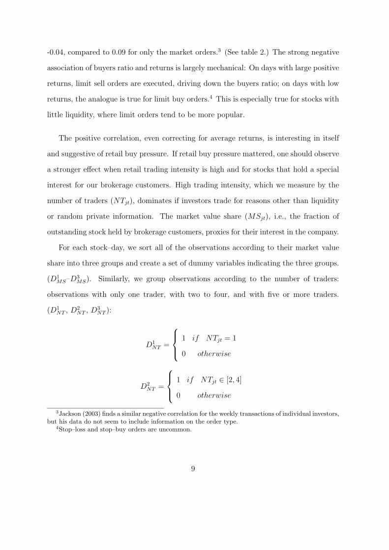
For each stock–day, we sort all of the observations according to their market value

share into three groups and create a set of dummy variables indicating the three groups.

(D1MS–D3

MS). Similarly, we group observations according to the number of traders:

observations with only one trader, with two to four, and with five or more traders.

(D1NT , D2

NT , D3NT ):

D1NT =

1 if NTjt = 1

0 otherwise

D2NT =

1 if NTjt ∈ [2, 4]

0 otherwise

3Jackson (2003) finds a similar negative correlation for the weekly transactions of individual investors,but his data do not seem to include information on the order type.

4Stop–loss and stop–buy orders are uncommon.

9

D3NT =

1 if NTjt ≥ 5

0 otherwise

Table 3 reviews the summary statistics for each of the nine NT/MS groups.

The differences in excess returns across groups are striking in their own right, varying

from -0.123 percent per day in the medium market–value–share group with one trader, to

2.316 in the top market–value–share group with more than 4 traders. (See table 3, lower

panel.) However, they do not capture the impact of buy pressure since buyers ratios are

not held constant. To address this issue, we estimate multivariate OLS regressions.

The baseline regression interacts the buyers ratio with both sets of dummy variables,

yielding nine parameter estimates for the sensitivity of returns to buy pressure:

rjt = α +3∑

k=1

3∑

l=1

βjtbrjtDkMSDl

NT + εjt (2)

The negative bias caused by the limit orders carries over to the regression results,

but even here a fundamental positive relationship between buyers ratio and returns is

discernible. The parameter estimates for (2) are shown in the first two columns of table

4. While most of the estimates are negative and significant, the estimate on brjt turns

positive for the groups that combine the top–two market value–share groups and the top

trading intensity group. The inclusion of stock fixed effects (column 2) magnifies this

result. Based on this estimate, a one–standard deviation increase of the buyers ratio

for an observation that falls into the top tercile in terms of market value share while

simultaneously being traded by at least 5 investors, increases the excess return by 0.48

percentage points.5

5For the standard deviation of the buyers ratio, see table 3; 0.232 ∗ 2.069 = 0.48

10

Repeating the regression without the limit–order observations reveals the full impact

of the buyers ratio. (See columns 3 and 4 in table 4). Except for observations falling into

the lowest market–value–share tercile, all of the coefficients are positive and statistically

significant. Furthermore, within all of the groups the estimates are monotonically in-

creasing, with the highest values in for the observations with a high market value share

and many traders. To illustrate the magnitude, a one–standard deviation increase in

the top group implies an abnormal return of almost 1.72 percentage points if we control

for stock fixed effects (column 4).

One explanation for this result could be intraday positive feedback trading. If in-

vestors buy after observing a high return earlier in the day, we would observe an increase

in the buyers ratio contemporaneously with high returns. Also, the buying would make

it more likely that an observation is placed into the top market value share group.

To dispel this doubt, we further subdivide our sample, according to the channel

used to place an order. Roughly speaking, investors have two choices. Either place an

ordinary order, which has to be received before 10am to be forwarded to the floor on the

same day, or trade directly via the Alternative Trading System. Only the latter allows

for serious intraday momentum trading. The last two columns in table 4 show separate

results for these two trading channels (termed “Ordinary Trades” and “Fast Trades”).

Contrary to the assertion, the buy pressure effect is actually stronger for ordinary trades

and weaker for trades executed through the Alternative Trading System.

Extensions

In table 5 we present a couple of extensions and robustness checks. All of the results are

based on the market–order sample.

In table 3 one could observe that average returns are substantially higher for stock–

days with a high number of traders or a high market value share. Concerned that the

11

interacted buyers ratio might just pick up this absolute difference, we re–specified the

regression to include the complete set of dummies in addition to the interaction. The

result (in column 1) shows that the coefficients in the lower two market value share

groups decrease somewhat, otherwise leaving the result unchanged.

In the next two columns, we first replace the stock–fixed effects with day fixed effects,

then include one lag of the excess return in the regression. Neither change affects the

size or direction of the coefficients in any substantial way.

The last column redefines the trading–intensity grouping. While the lowest group

remains unchanged at NTjt = 1, the medium/high cutoff changes to 8, placing only

observations with NTjt ≥ 9 into the top group. This change increases the coefficient on

buyers ratios for the highest NTjt/MSjt classification substantially, from 6.933 to 9.221.

Future returns

In the last table we take a look at the predictive power of the buyers ratio for returns

up to three days into the future.

For the return on the next day, it seems that the effect of the previous day’s buy

pressure continues, albeit with a smaller magnitude. The coefficient on the buyers ratio

in the top group of 1.186 predicts an abnormal return of 0.29 percentage points on the

next trading day for a one–standard–deviation increase in the buyers ratio. The subse-

quent days see some return reversal. The same coefficient becomes -0.562, but is only

marginally significant. There are more signs for reversal among the other coefficients,

the pattern does not seem to be related to the NT/MS–grouping, however.

Including the same–day and/or lagged excess returns does not alter these findings.

(Not shown.)

12

5 Conclusion

Contributing to the literature on herding which has focused on institutional investors,

this study not only documents substantial herding among individual investors, but can

also establishes a strong and stable positive relationship between retail buy pressure

and excess returns at a daily frequency. On a technical note, the findings illustrate

the importance of distinguishing between market orders and limit orders as the latter

introduce a spurious negative correlation between retail buy pressure and returns.

Of course, the usual caveats apply. The brokerage customers may not be representa-

tive of the average individual investor, although the return results suggest so. Moreover,

the German boom years of 1999-2000 don’t exactly represent “normal times” for stock

markets.

If the documented behavior generalizes across time and markets, one question emerges:

how does this fit in with the accrued evidence of a positive correlation between returns

and institutional buying? There is no evidence for German institutional investors, but

if they exhibit this positive correlation as well, who takes the other side of the trade?

While this question remains open for now, some envisioned future research may shed

some light. The documented behavior does not explain why individuals herd or, for

that matter, trade at all. One extension, under work, explores persistence in retail

buy pressure and its relation to past returns. There is some preliminary evidence that

herding is even more pronounced in foreign stocks which may imply that attention plays

an important role in triggering herding. Perhaps individual investors tend to react more

to extreme news and information about foreign stocks needs to be more extreme to be

reported, or foreign stock signals are more highly correlated because there is a smaller

number of information outlets that individual investors pay attention to. In a second

extension, studying the temporal aspects of herding and extending the return results to

13

different time horizons has the potential of illuminating the causes of herding.

Another interesting extension explores the profitability of a trading strategy that

consists of buying the stocks most aggressively bought and shorting the stocks most

aggressively sold by retail investors. This should clarify if the arbitrage opportunities

implied by the predictive power of retail buying are economically significant or merely

a statistical artefact.

14

References

Barber, B. M. and Odean, T. (2002). All that Glitters: The Effect of Attention and Newson the Buying Behavior of Individual and Institutional Investors. Working Paper.

Barber, B. M., Odean, T. and Zhu, N. (2002). Systematic noise.

Barberis, N. C. and Shleifer, A. (2002). Style Investing, Journal of Financial Economics. Forthcoming.

De Long, J. B., Shleifer, A., Summers, L. and Waldmann, R. J. (1990). Noise traderrisk in financial markets, Journal of Political Economy 98(4): 703–738.

Dorn, D. (2002). Does sentiment drive the retail demand for IPOs? Working Paper,Columbia Business School.

Griffin, J. M., Harris, J. and Topaloglu, S. (2003). The dynamics of institutional andindividual trading, Journal of Finance . Forthcoming.

Jackson, A. (2003). The aggregate behaviour of individual investors. London BusinessSchool, Working Paper.

Kumar, A. (2002). Style switching and stock returns. Working Paper, Cornell University.

Lakonishok, J., Shleifer, A. and Vishny, R. W. (1992). The impact of institutionaltrading on stock prices, Journal of Financial Economics 32: 23–43.

Lee, C., Shleifer, A. and Thaler, R. (1991). Investor sentiment and the closed-end fundpuzzle, Journal of Finance 46: 75–109.

Nofsinger, J. R. and Sias, R. W. (1999). Herding and feedback trading by institutionaland individual investors, Journal of Finance 54(6): 2263 – 2295.

Odean, T. (1998). Are investors reluctant to realize their losses?, Journal of Finance53(5): 1775–1798.

Ofek, E. and Richardson, M. (2003). DotCom mania: The rise and fall of internet stockprices, Journal of Finance . Forthcoming.

Shleifer, A. (2000). Inefficient markets: an introduction to behavioral finance, OxfordU. Press, Oxford.

Wermers, R. (1999). Mutual fund herding and the impact on stock prices, Journal ofFinance 54(2): 581–622.

Wylie, S. (2002). Fund manager herding: A test of the accuracy of empirical resultsusing UK data. Working Paper, The Tuck School at Dartmouth.

15

Table 1: The LSV measure of Herding

This table summarizes the means of the herding measure by Lakonishok et al. (1992)(LSV), as described in the text. Rows show the measure, in percent, for different levelsof trading activity, measured by the number of traders (NTjt) by stock-day observation.On the left hand side of the table, we show the results for the entire sample (includingboth limit and market orders), on the right hand side only for market orders. Theupper panel shows the result using data on the daily frequency, the lower on a quarterlyfrequency.All estimates are significant on conventional significance levels.

Market and Limit Orders Only Market Orders

Daily Data

Mean(LSV) Observations Mean(LSV) Observations

NTjt in [2,4] 3.12 23,816 3.02 15,303

NTjt >= 2 4.71 37,389 4.43 21,985

NTjt >= 5 6.74 13,573 6.27 6,682

NTjt >= 10 8.74 5,060 7.25 2,242

Quarterly Data

Mean(LSV) Observations Mean(LSV) Observations

NTjt in [2,4] 3.50 697 1.22 618

NTjt >= 2 6.41 3,138 4.82 2,379

NTjt >= 5 7.06 2,441 5.52 1,761

NTjt >= 10 7.34 1,907 5.93 1,332

16

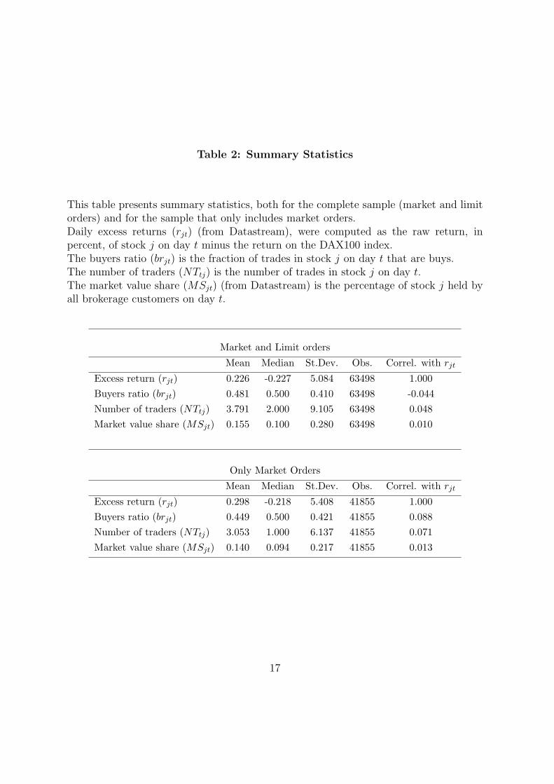
Table 2: Summary Statistics

This table presents summary statistics, both for the complete sample (market and limitorders) and for the sample that only includes market orders.Daily excess returns (rjt) (from Datastream), were computed as the raw return, inpercent, of stock j on day t minus the return on the DAX100 index.The buyers ratio (brjt) is the fraction of trades in stock j on day t that are buys.The number of traders (NTtj) is the number of trades in stock j on day t.The market value share (MSjt) (from Datastream) is the percentage of stock j held byall brokerage customers on day t.

Market and Limit orders

Mean Median St.Dev. Obs. Correl. with rjt

Excess return (rjt) 0.226 -0.227 5.084 63498 1.000Buyers ratio (brjt) 0.481 0.500 0.410 63498 -0.044Number of traders (NTtj) 3.791 2.000 9.105 63498 0.048Market value share (MSjt) 0.155 0.100 0.280 63498 0.010

Only Market Orders

Mean Median St.Dev. Obs. Correl. with rjt

Excess return (rjt) 0.298 -0.218 5.408 41855 1.000Buyers ratio (brjt) 0.449 0.500 0.421 41855 0.088Number of traders (NTtj) 3.053 1.000 6.137 41855 0.071Market value share (MSjt) 0.140 0.094 0.217 41855 0.013

17

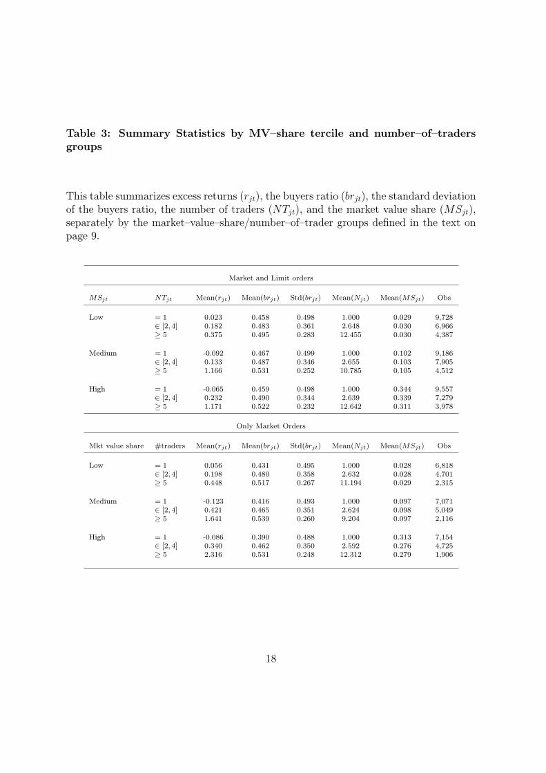
Table 3: Summary Statistics by MV–share tercile and number–of–tradersgroups

This table summarizes excess returns (rjt), the buyers ratio (brjt), the standard deviationof the buyers ratio, the number of traders (NTjt), and the market value share (MSjt),separately by the market–value–share/number–of–trader groups defined in the text onpage 9.

Market and Limit orders

MSjt NTjt Mean(rjt) Mean(brjt) Std(brjt) Mean(Njt) Mean(MSjt) Obs

Low = 1 0.023 0.458 0.498 1.000 0.029 9,728∈ [2, 4] 0.182 0.483 0.361 2.648 0.030 6,966≥ 5 0.375 0.495 0.283 12.455 0.030 4,387

Medium = 1 -0.092 0.467 0.499 1.000 0.102 9,186∈ [2, 4] 0.133 0.487 0.346 2.655 0.103 7,905≥ 5 1.166 0.531 0.252 10.785 0.105 4,512

High = 1 -0.065 0.459 0.498 1.000 0.344 9,557∈ [2, 4] 0.232 0.490 0.344 2.639 0.339 7,279≥ 5 1.171 0.522 0.232 12.642 0.311 3,978

Only Market Orders

Mkt value share #traders Mean(rjt) Mean(brjt) Std(brjt) Mean(Njt) Mean(MSjt) Obs

Low = 1 0.056 0.431 0.495 1.000 0.028 6,818∈ [2, 4] 0.198 0.480 0.358 2.632 0.028 4,701≥ 5 0.448 0.517 0.267 11.194 0.029 2,315

Medium = 1 -0.123 0.416 0.493 1.000 0.097 7,071∈ [2, 4] 0.421 0.465 0.351 2.624 0.098 5,049≥ 5 1.641 0.539 0.260 9.204 0.097 2,116

High = 1 -0.086 0.390 0.488 1.000 0.313 7,154∈ [2, 4] 0.340 0.462 0.350 2.592 0.276 4,725≥ 5 2.316 0.531 0.248 12.312 0.279 1,906

18

Table

4:

Herd

ing

and

Retu

rns

This

table

report

sth

ere

sult

sof

are

gre

ssio

nof

the

exce

ssre

turn

of

stock

jon

day

t(r

jt,in

per

cent,

com

pute

dover

the

DA

X100)

on

the

buyer

sra

tio

brjt,w

ith

the

buyer

sra

tio

fully

inte

ract

edw

ith

dum

my

vari

able

sin

dic

ati

ng

mark

et-v

alu

esh

are

terc

iles

(D1 M

S−

D3 M

S)

and

dum

mie

sin

dic

ati

ng

the

num

ber

–of–

trader

sgro

ups

(D1 N

Tfo

robse

rvati

ons

wit

honly

one

trader

,D

2 NT

wit

htw

oto

four

trader

s,and

D3 N

Tfive

or

more

trader

s).

The

mark

etvalu

esh

are

MS

kw

as

com

pute

das

the

num

ber

of

stock

shel

dby

all

bro

ker

age

cust

om

ers

div

ided

by

the

tota

louts

tandin

gst

ock

,fr

om

Data

stre

am

.“O

rdin

ary

trades

”are

all

trades

not

pla

ced

thro

ugh

the

Alt

ernati

ve

Tra

din

gSyst

em,

“Fast

Tra

des

”are

transa

ctio

ns

thro

ugh

the

Alt

ernati

ve

Tra

din

gSyst

em,

whic

hallow

sfo

rim

med

iate

quote

sand

transa

ctio

ns.

The

num

ber

ofobse

rvati

ons

for

the

two

tradin

gch

annel

sdoes

not

add

toth

eto

talfo

r“O

nly

Mark

etO

rder

s”bec

ause

on

agiv

enst

ock

–day,

ther

em

ay

be

both

“ord

inary

trades

”and

“fa

sttr

ades

”.

Dep

enden

tV

ari

able

:r j

t

Sam

ple

:M

ark

etand

Lim

itO

rder

sO

nly

Mark

etO

rder

s

All

Mark

etO

rder

sO

rdin

ary

Tra

des

Fast

Tra

des

coeff

seco

effse

coeff

seco

effse

coeff

seco

effse

brjt∗D

1 MS∗D

1 NT

-0.6

92

(0.0

7)*

*-0

.884

(0.0

8)*

*0.5

66

(0.1

1)*

*0.1

96

(0.1

1)+

0.5

48

(0.1

2)*

*-0

.459

(0.1

6)*

*

brjt∗D

1 MS∗D

2 NT

-0.7

48

(0.1

0)*

*-0

.835

(0.1

2)*

*0.5

82

(0.1

7)*

*0.3

02

(0.2

1)

0.9

72

(0.2

1)*

*-0

.407

(0.2

5)+

brjt∗D

1 MS∗D

3 NT

-0.7

08

(0.2

1)*

*-0

.532

(0.2

9)+

0.9

76

(0.3

8)*

1.0

53

(0.5

4)+

1.5

12

(0.4

1)*

*0.2

54

(0.5

8)

brjt∗D

2 MS∗D

1 NT

-0.6

86

(0.0

8)*

*-0

.709

(0.0

8)*

*0.6

63

(0.1

1)*

*0.5

92

(0.1

2)*

*1.2

44

(0.1

5)*

*-0

.402

(0.2

1)+

brjt∗D

2 MS∗D

2 NT

-0.5

24

(0.1

3)*

*-0

.417

(0.1

4)*

*1.7

24

(0.1

9)*

*1.8

22

(0.2

2)*

*2.4

12

(0.2

8)*

*1.1

72

(0.2

7)*

*

brjt∗D

2 MS∗D

3 NT

0.9

00

(0.3

5)*

1.4

34

(0.3

7)*

*3.5

39

(0.7

1)*

*4.3

41

(0.6

8)*

*4.0

58

(0.8

4)*

*3.9

03

(0.8

8)*

*

brjt∗D

3 MS∗D

1 NT

-0.7

14

(0.0

7)*

*-0

.778

(0.0

9)*

*0.9

53

(0.1

3)*

*1.0

44

(0.1

3)*

*1.7

80

(0.1

7)*

*0.0

20

(0.1

9)

brjt∗D

3 MS∗D

2 NT

-0.4

36

(0.1

4)*

*-0

.181

(0.1

6)

1.9

27

(0.2

2)*

*2.5

02

(0.2

4)*

*3.5

09

(0.3

3)*

*1.4

28

(0.3

2)*

*

brjt∗D

3 MS∗D

3 NT

1.3

01

(0.3

9)*

*2.0

69

(0.4

5)*

*5.5

45

(0.8

1)*

*6.9

33

(0.9

0)*

*7.8

44

(1.2

9)*

*5.6

94

(1.0

9)*

*

Const

ant

0.4

13

(0.0

4)*

*0.3

65

(0.0

4)*

*-0

.339

(0.0

5)*

*-0

.392

(0.0

6)*

*-0

.465

(0.0

5)*

*0.1

12

(0.1

0)

Sto

ckfixed

effec

ts?

no

yes

no

yes

yes

yes

adj.

R2

0.0

07

0.0

11

0.0

24

0.0

31

0.0

39

0.0

27

Obse

rvati

ons

63498

63498

41855

41855

31167

20764

Het

erosc

edast

icity–ro

bust

standard

erro

rssh

ow

nin

pare

nth

esis

.T

hes

est

andard

erro

rsallow

for

free

corr

elati

on

of

the

resi

duals

wit

hin

sam

e–st

ock

obse

rvati

ons.

Sta

tist

icalsi

gnifi

cance

on

the

1/5/10%

level

are

indic

ate

dby

**/*/+

19

Table

5:

Herd

ing

and

Retu

rns:

Robust

ness

This

table

report

sth

ere

sult

sof

are

gre

ssio

nof

the

exce

ssre

turn

of

stock

jon

day

t(r

jt,in

per

cent,

com

pute

dover

the

DA

X100)

on

the

buyer

sra

tio

brjt,w

ith

the

buyer

sra

tio

fully

inte

ract

edw

ith

dum

my

vari

able

sin

dic

ati

ng

mark

et-v

alu

esh

are

terc

iles

(D1 M

S−

D3 M

S)

and

dum

mie

sin

dic

ati

ng

the

num

ber

–of–

trader

sgro

ups

(D1 N

Tfo

robse

rvati

ons

wit

honly

one

trader

,D

2 NT

wit

htw

oto

four

trader

s,and

D3 N

Tfive

or

more

trader

s).

The

mark

etvalu

esh

are

MS

jt

was

com

pute

das

the

num

ber

of

stock

shel

dby

all

bro

ker

age

cust

om

ers

div

ided

by

the

tota

louts

tandin

gst

ock

,fr

om

Data

stre

am

.In

the

firs

tco

lum

n,la

bel

led

“in

cludin

gall

dum

mie

s”,w

ein

clude

all

ofth

eabove

dum

mie

sin

addit

ion

toth

ein

tera

ctio

nw

ith

the

buyer

sra

tio.

(coeffi

cien

tsnot

show

n)

Inth

ese

cond

colu

mn,la

bel

led

“w

ith

day

fixed

effec

ts”,w

ere

pla

ceth

eco

mpany

fixed

effec

tw

ith

day

fixed

effec

ts.

(coeffi

cien

tsnot

show

n)

Inth

eth

ird

colu

mn,la

bel

led

“w

ith

lagged

retu

rns”

,w

eadd

the

exce

ssre

turn

ofst

ock

jon

the

pre

vio

us

tradin

gday.

(rjt−

1)

Inth

efo

urt

hco

lum

n,la

bel

led

“sm

aller

top-N

T-g

roup”,w

ere

defi

ne

the

num

ber

–of–

trader

gro

ups

tobe

D1 N

Tfo

robse

rvati

ons

wit

honly

one

trader

,D

2 NT

wit

htw

oto

eight

trader

s,and

D3 N

Tnin

eor

more

trader

s.

All

regre

ssio

ns

are

base

don

transa

ctio

ns

that

wer

em

ark

etord

ers.

Dep

enden

tV

ari

able

:r j

t

Vari

ati

on:

incl

udin

gall

dum

mie

sw

ith

day

fixed

effec

tsw

ith

lagged

retu

rns

smaller

top-N

T-g

roup

coeff

seco

effse

coeff

seco

effse

r jt−

10.0

26

(0.0

1)*

*

brjt∗D

1 MS∗D

1 NT

0.2

90

(0.1

2)*

0.5

40

(0.1

0)*

*0.1

90

(0.1

1)+

0.1

90

(0.1

1)+

brjt∗D

1 MS∗D

2 NT

-0.4

62

(0.2

2)+

0.5

06

(0.1

6)*

*0.3

20

(0.2

0)+

0.4

07

(0.2

4)+

brjt∗D

1 MS∗D

3 NT

-1.1

62

(0.5

2)+

0.8

97

(0.3

6)*

1.0

51

(0.5

4)+

0.8

61

(0.5

1)+

brjt∗D

2 MS∗D

1 NT

0.7

95

(0.1

3)*

*0.6

41

(0.1

1)*

*0.6

08

(0.1

2)*

*0.5

83

(0.1

2)*

*

brjt∗D

2 MS∗D

2 NT

1.8

05

(0.2

8)*

*1.6

47

(0.1

9)*

*1.8

07

(0.2

1)*

*2.1

58

(0.2

4)*

*

brjt∗D

2 MS∗D

3 NT

2.5

03

(1.2

5)+

3.4

25

(0.6

8)*

*4.3

01

(0.6

7)*

*5.3

73

(1.2

9)*

*

brjt∗D

3 MS∗D

1 NT

1.1

67

(0.1

3)*

*0.9

27

(0.1

3)*

*1.0

43

(0.1

3)*

*1.0

40

(0.1

3)*

*

brjt∗D

3 MS∗D

2 NT

2.7

01

(0.3

1)*

*1.8

06

(0.2

1)*

*2.4

30

(0.2

4)*

*3.0

10

(0.2

7)*

*

brjt∗D

3 MS∗D

3 NT

7.7

94

(1.7

2)*

*5.3

51

(0.7

8)*

*6.5

50

(0.8

6)*

*9.2

21

(1.6

6)*

*

Const

ant

-0.1

31

(0.1

3)

-0.3

09

(0.0

5)*

*-0

.390

(0.0

6)*

*-0

.368

(0.0

6)*

*

Sto

ckfixed

effec

ts?

yes

no

yes

yes

adj.

R2

0.0

33

0.0

69

0.0

31

0.0

30

Obse

rvati

ons

41855

41855

41322

41855

Het

erosc

edast

icity–ro

bust

standard

erro

rssh

ow

nin

pare

nth

esis

.T

hes

est

andard

erro

rsallow

for

free

corr

elati

on

of

the

resi

duals

wit

hin

sam

e–st

ock

obse

rvati

ons.

Sta

tist

icalsi

gnifi

cance

on

the

1/5/10%

level

are

indic

ate

dby

**/*/+

20

Table

6:

Herd

ing

and

Futu

reR

etu

rns

Res

ult

sofa

regre

ssio

nofth

eex

cess

retu

rns

one,

two,and

thre

e(t

radin

g)

days

into

toth

efu

ture

,on

the

buyer

sra

tio

inte

ract

edw

ith

the

nin

edum

mie

sin

dic

ati

ng

thre

em

ark

et–valu

e–sh

are

terc

iles

and

thre

enum

ber

–of–

trader

gro

ups.

See

Table

4fo

ra

more

det

ailed

des

crip

tion.

Dep

enden

tVari

able

:

r jt+

1r j

t+2

r jt+

3

coeff

seco

effse

coeff

se

brjt∗D

1 MS∗D

1 NT

0.4

94

(0.1

1)*

*0.0

26

(0.0

9)

0.1

29

(0.0

9)

brjt∗D

1 MS∗D

2 NT

0.4

54

(0.1

3)*

*0.1

00

(0.1

2)

-0.1

04

(0.1

2)

brjt∗D

1 MS∗D

3 NT

0.5

74

(0.2

0)*

*0.3

03

(0.1

6)+

-0.2

44

(0.1

5)

brjt∗D

2 MS∗D

1 NT

0.4

10

(0.0

9)*

*0.1

70

(0.1

0)+

-0.4

00

(0.0

9)*

*

brjt∗D

2 MS∗D

2 NT

0.5

70

(0.1

5)*

*0.0

13

(0.1

8)

-0.1

87

(0.1

4)

brjt∗D

2 MS∗D

3 NT

1.3

62

(0.3

6)*

*-0

.627

(0.3

1)*

-0.7

23

(0.2

7)*

*

brjt∗D

3 MS∗D

1 NT

0.4

29

(0.1

1)*

*-0

.165

(0.1

1)

-0.1

71

(0.1

1)

brjt∗D

3 MS∗D

2 NT

1.1

10

(0.1

8)*

*-0

.274

(0.1

6)+

-0.6

69

(0.1

7)*

*

brjt∗D

3 MS∗D

3 NT

1.1

86

(0.3

2)*

*-0

.219

(0.2

8)

-0.5

62

(0.3

0)+

Const

ant

-0.1

65

(0.0

3)*

*0.0

99

(0.0

3)*

*0.2

15

(0.0

3)*

*

Sto

ckfixed

effec

ts?

yes

yes

yes

adj.

R2

0.0

04

-0.0

00

0.0

01

Obse

rvati

ons

41246

40960

40830

Het

erosc

edast

icity–ro

bust

standard

erro

rssh

ow

nin

pare

nth

esis

.T

hes

est

andard

erro

rsallow

for

free

corr

elati

on

of

the

resi

duals

wit

hin

sam

e–st

ock

obse

rvati

ons.

Sta

tist

icalsi

gnifi

cance

on

the

1/5/10%

level

are

indic

ate

dby

**/*/+

21