heterogeneous firms, the structure of industry, & trade ... · heterogeneous firms, the...
TRANSCRIPT

Heterogeneous Firms, the Structure of Industry, & Trade under Oligopoly
by
Eddy BEKKERS Joseph FRANCOIS*)
Working Paper No. 0811 August 2008
DDEEPPAARRTTMMEENNTT OOFF EECCOONNOOMMIICCSSJJOOHHAANNNNEESS KKEEPPLLEERR UUNNIIVVEERRSSIITTYY OOFF
LLIINNZZ
Johannes Kepler University of LinzDepartment of Economics
Altenberger Strasse 69 A-4040 Linz - Auhof, Austria
www.econ.jku.at
*)[email protected] phone +43 (0)70 2468 -8239, -8238 (fax)

Heterogeneous Firms, the Structure of Industry,
& Trade under Oligopoly ∗
Eddy Bekkers
University of Linz
Joseph Francois
University of Linz
& CEPR (London)
ABSTRACT: We develop a model with endogeneity in key features of industrial structurelinked to heterogeneous cost structures under Cournot competition. We use the model toexplore issues related to cross-country differences in industry structure and the impact ofglobalization on markups and pricing, concentration, and productivity. The model neststwo workhorse trade models, the Brander & Krugman reciprocal dumping model and theRicardian technology-based trade model, as special cases. We examine both free entry andlimited entry (free exit) cases. The model generates clear testable predictions on the proba-bility of zero trade flows and the pattern of export prices, and on cross-country and industryvariations in industrial structure controlling for openness. Market prices decline as a resultof trade liberalization, the least productive firms get squeezed out of the market, exportingfirms gain market share, and more firms become trade oriented. In addition, depending onthe strength of underlying cost heterogeneity, falling prices are consistent with both increas-ing and falling industry concentration following episodes of integration. Welfare rises withtrade liberalization, unless trade costs decline from a prohibitive level in the short run freeexit case. Variation across industries and markets in markups, concentration, and pricingstructures is otherwise a function of market size and the variation in cost heterogeneity acrossindustries.
Keywords: Firm heterogeneity, Cournot competition, Composition effects of trade liberal-ization
JEL codes: L11, L13, F12
printdate: August 27, 2008
∗Thanks are due to participants in Tinbergen Institue and CEPR workshops and the ETSG annualmeetings. Address for correspondence: Univ. Prof. Dr. J. Francois, Johannes Kepler University Linz,Department of Economics, Altenbergerstraße 69, A - 4040 Linz, AUSTRIA. email: [email protected],web:www.i4ide.org/francois/

Heterogeneous Firms, the Structure of Industry,& Trade under Oligopoly
ABSTRACT: We develop a model with endogeneity in key features of industrial struc-ture linked to heterogeneous cost structures under Cournot competition. We use the modelto explore issues related to cross-country differences in industry structure and the impactof globalization on markups and pricing, concentration, and productivity. The model neststwo workhorse trade models, the Brander & Krugman reciprocal dumping model and theRicardian technology-based trade model, as special cases. We examine both free entry andlimited entry (free exit) cases. The model generates clear testable predictions on the proba-bility of zero trade flows and the pattern of export prices, and on cross-country and industryvariations in industrial structure controlling for openness. Market prices decline as a resultof trade liberalization, the least productive firms get squeezed out of the market, exportingfirms gain market share, and more firms become trade oriented. In addition, depending onthe strength of underlying cost heterogeneity, falling prices are consistent with both increas-ing and falling industry concentration following episodes of integration. Welfare rises withtrade liberalization, unless trade costs decline from a prohibitive level in the short run freeexit case. Variation across industries and markets in markups, concentration, and pricingstructures is otherwise a function of market size and the variation in cost heterogeneity acrossindustries.
keywords: Firm heterogeneity, Cournot competition, effects of trade liberalization
JEL codes: L11, L13, F12.
1 Introduction
Research on the impact of globalization on firms has shown that the reallocation effects of
trade are an important mechanism linking openness to productivity. Bernard and Jensen
(2004) find that almost half of the rise of manufacturing total factor productivity in the USA
between 1983 and 1992 is linked to a reallocation effect of resources towards more productive
and trade oriented firms. Episodes of liberalization in developing countries also show the
importance of changes in firm composition – composition effects (Tybout 2001).
A number of models of heterogeneous productivity have been put forward in the recent
theoretical trade literature to explain composition effects of trade. A standard result is that
processes of firm formation involving heterogeneous cost structures across firms imply bene-
ficial reallocation effects from trade liberalization linked to rationalization of the population
of firms. Less efficient firms producing for the domestic market are squeezed out by more
efficient trading firms. For example, Melitz (2003) introduces heterogeneous productivity
in a monopolistic competition framework with CES-preferences, while Bernard, et al (2003)
include heterogeneous productivity in a model with Bertrand competition. Working with
1

monopolistic competition models, Baldwin and Robert-Nicoud (2008) examine linkages be-
tween trade and growth given firm heterogeneity, while Ghironi and Melitz (2007) examine
macroeconomic dynamics. In contrast, in this paper we explore heterogeneous productivity
in a model with oligopoly characterized by Cournot competition. Basic aspects of market
structure – markups, industrial concentration, relative firm positions, and prices for domes-
tic and export markets – are endogenous. They depend on the interaction between the
technology set, market size, and trade openness.
The model we develop is a two-country, multi-sector model of trade under Cournot com-
petition.1 The value added of this approach is threefold. First, the model is parsimonious,
while generating a rich set of results linked to composition effects. This includes welfare
effects of trade liberalization and the endogeneity of market structure. Moreover, we do not
need to assume a specific distribution of productivity, as is the case with Bernard, et al
(2003) and Melitz and Ottaviano (2008), to generate our results. Second, the model nests
two workhorse trade models, the Brander and Krugman (1983) reciprocal dumping model
and the Ricardian model, as special cases. Third, the model generates clear testable predic-
tions on the probability of zero trade flows and export prices, as well as predictions about
linkages between openness and industrial market structure across industries and countries.
The pattern of zeros and unit values has emerged as a particularly important issue in the
recent empirical trade literature. (See Baldwin and Harrigan 2007, Baldwin and Taglioni
2006). In the model developed here, a larger distance between countries leads to a higher
probability of zero trade flows and lower fob export prices. The size of the importer country
also influences the probability of zero trade flows and decreases the fob export price. A
number of other results stand out. In the free entry case, falling trade costs raise welfare
unambiguously. However, in the case without free entry, welfare increases as well only when
certain conditions are placed on the distribution of costs. In addition, falling prices from
trade liberalization can go hand and hand with increased firm concentration. Finally, we
note the possibility of delocation effects with heterogeneous countries. Unilateral liberaliza-
tion then leads to higher market prices in the liberalizing country. All results are derived
without specifying a specific distribution of costs. Preferences are assumed to be CES.
The paper is organized as follows. In Section 2 we lay out the basic model. Section 31Van Long et al. (2007) also address firm heterogeneity in an oligopoly model. Their paper is focused on
a different set of issues however, the interaction of trade and R&D.
2
goes into the case of trade without free entry and section 4 addresses the case of trade with
free entry. Section 5 explores the heterogeneous countries case. Section 6 concludes.
2 The Basic Model
This section lays out the basics of the model without trade (or identically for an integrated or
single global economy without trade costs). Industrial concentration emerges endogenously
as a function of the degree of firm heterogeneity and market size, while the relationship of
concentration to price depends on the cost structure of industry.
We start by assume that there are Q+ 1 sectors in the economy, oligopolistic Q sectors
producing qj and 1 sector producing z under conditions of perfect competition. In the first
sections it is assumed that the Cournot sectors are symmetric. Later on this assumption is
relaxed when asymmetries in national technology sets, country size, and policy are explored.
Throughout it is assumed that there are sufficient sectors in the economy so that the effect
of a price change on demand through the price index is negligible for firms. (There is no
numeraire problem). There are L equal agents each supplying 1 unit of labor. All profit
income from the Cournot sectors goes to the economic agents. The utility function of each
agent is CES. The optimization problem of the consumer generates the following market
demand functions in the Cournot sectors qj and in the perfect competition sector z:
qj =IP σ−1
U
pσj(1)
z = IP σ−1U (2)
The price of good z is normalized at 1 and I is the endogenous income of all agents, the
sum of labor and profit income. PU is the consumer price index, corresponding to one unit
of utility:
PU =
Q∑j=1
p1−σj + 1
11−σ
=[Qp1−σ + 1
] 11−σ (3)
Until we relax out symmetry assumptions, we will focus on one representative Cournot sector.
(We will warn the reader when we drop these assumptions.) This means we can drop the
sector index j for now. Labor is the only factor of production and there is a labor force of
size L. One unit of labor is needed to produce one unit of the perfect competition good y.
3

This means the wage is equal to 1. In the q sectors productivity is heterogeneous. One unit
of labor can be transformed into 1/ci units of q for the i-th firm which has marginal cost of
production ci. There are no fixed costs of production. Therefore the cost function of firm i
is given by
Ci (qi) = ciqi (4)
There is Cournot competition between the different firms in the q-sectors. So, firms maximize
profits towards quantity supplied, taking the quantity supplied by other firms as given. Profit
of firm i is given by:
πi = pqi − ciqi (5)
The first order condition is defined as:
∂πi∂qi
= p
[1− 1
σ
qiq
]− ci = 0 (6)
With q =n∑i=1
qi. n is the number of firms in the market. Using the first order condition, the
second order condition can be written as follows (derivation in appendix A):
− 1σ
p
q
[(σ + 1) ci − (σ − 1) p
p
]< 0 (7)
Using the definition for market share, θi = qiq , the first order condition can be rewritten as:
p
(1− θi
σ
)= ci (8)
θi = σp− cip
(9)
The marginal revenues on the LHS of equation (9) should be at least as large as the marginal
costs on the RHS. The larger is market share θi, the lower is marginal revenue. So, for positive
sales (θi ≥ 0) which are implicitly imposed, a firm can satisfy the FOC by just reducing its
market share as long as its marginal cost is smaller than the market price. There is a cutoff
cost level c∗ with which a firm would just stay in the market. This cutoff cost level c∗ is
equal to the market price p. The highest cost firm staying in the market has a cost level
equal or just below the cutoff cost level and selling an amount just above zero.
The equilibrium price and quantities sold can be found for a given number of firms. Below
4
a free entry condition is added to endogenise the number of firms. Suppose for now there
are n firms. Combining the demand equation in (1) with n first order conditions in equation
(6) and with the equation for the sum of market shares, one can find the following solutions
for the market price p, total sector sales q and sales of an individual firm qi:
p =σ
σn− 1
n∑i=1
ci =σn
σn− 1c (10)
q =IP σ−1
U
cσ
(σn− 1σn
)σ(11)
qi = σIP σ−1U
c− cicσ
(σn− 1σn
)σ−1
(12)
with c the average cost of firms, c = 1n
n∑i=1
ci.
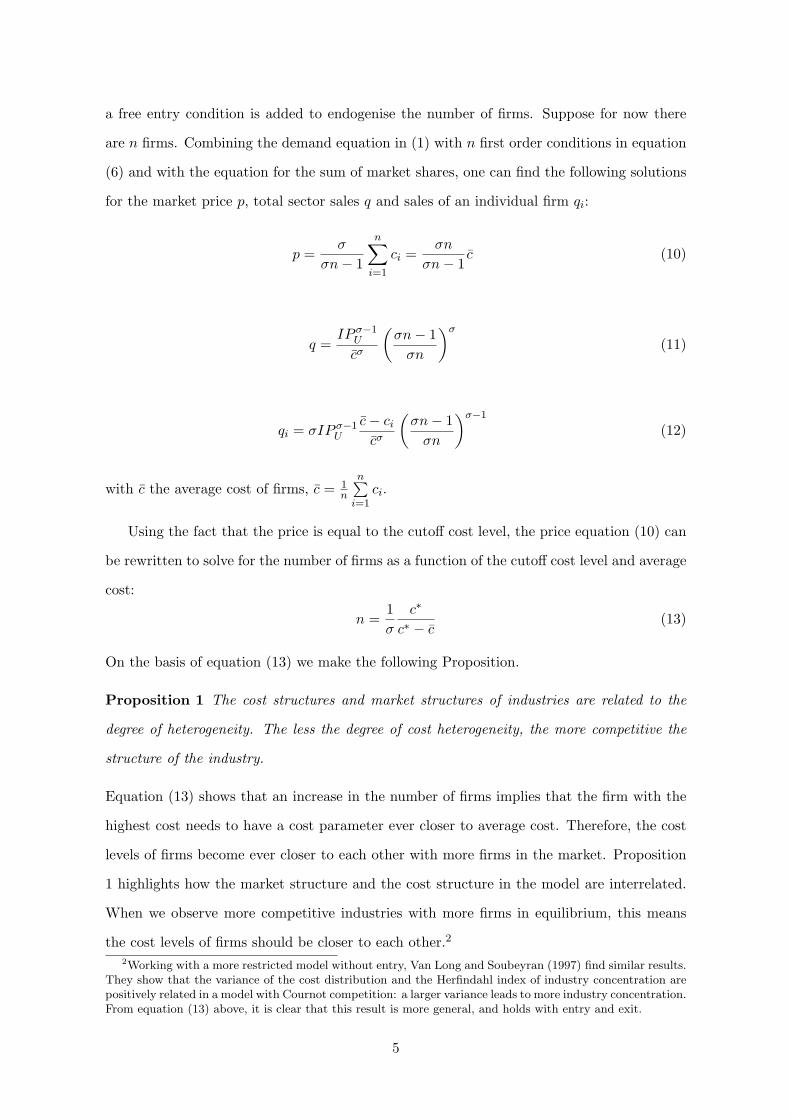
Using the fact that the price is equal to the cutoff cost level, the price equation (10) can
be rewritten to solve for the number of firms as a function of the cutoff cost level and average
cost:
n =1σ
c∗
c∗ − c(13)
On the basis of equation (13) we make the following Proposition.
Proposition 1 The cost structures and market structures of industries are related to the
degree of heterogeneity. The less the degree of cost heterogeneity, the more competitive the
structure of the industry.
Equation (13) shows that an increase in the number of firms implies that the firm with the
highest cost needs to have a cost parameter ever closer to average cost. Therefore, the cost
levels of firms become ever closer to each other with more firms in the market. Proposition
1 highlights how the market structure and the cost structure in the model are interrelated.
When we observe more competitive industries with more firms in equilibrium, this means
the cost levels of firms should be closer to each other.2
2Working with a more restricted model without entry, Van Long and Soubeyran (1997) find similar results.They show that the variance of the cost distribution and the Herfindahl index of industry concentration arepositively related in a model with Cournot competition: a larger variance leads to more industry concentration.From equation (13) above, it is clear that this result is more general, and holds with entry and exit.
5
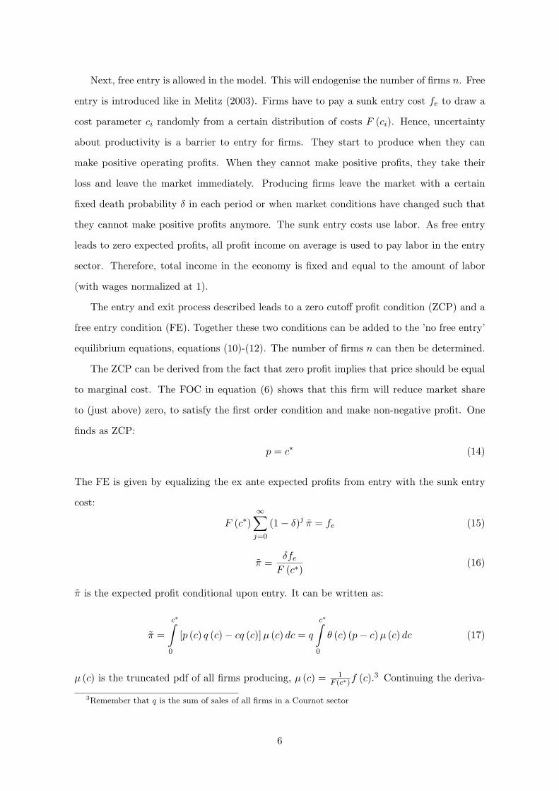
Next, free entry is allowed in the model. This will endogenise the number of firms n. Free
entry is introduced like in Melitz (2003). Firms have to pay a sunk entry cost fe to draw a
cost parameter ci randomly from a certain distribution of costs F (ci). Hence, uncertainty
about productivity is a barrier to entry for firms. They start to produce when they can
make positive operating profits. When they cannot make positive profits, they take their
loss and leave the market immediately. Producing firms leave the market with a certain
fixed death probability δ in each period or when market conditions have changed such that
they cannot make positive profits anymore. The sunk entry costs use labor. As free entry
leads to zero expected profits, all profit income on average is used to pay labor in the entry
sector. Therefore, total income in the economy is fixed and equal to the amount of labor
(with wages normalized at 1).
The entry and exit process described leads to a zero cutoff profit condition (ZCP) and a
free entry condition (FE). Together these two conditions can be added to the ’no free entry’
equilibrium equations, equations (10)-(12). The number of firms n can then be determined.
The ZCP can be derived from the fact that zero profit implies that price should be equal
to marginal cost. The FOC in equation (6) shows that this firm will reduce market share
to (just above) zero, to satisfy the first order condition and make non-negative profit. One
finds as ZCP:
p = c∗ (14)
The FE is given by equalizing the ex ante expected profits from entry with the sunk entry
cost:
F (c∗)∞∑j=0
(1− δ)j π = fe (15)
π =δfeF (c∗)
(16)
π is the expected profit conditional upon entry. It can be written as:
π =
c∗∫0
[p (c) q (c)− cq (c)]µ (c) dc = q
c∗∫0
θ (c) (p− c)µ (c) dc (17)
µ (c) is the truncated pdf of all firms producing, µ (c) = 1F (c∗)f (c).3 Continuing the deriva-
3Remember that q is the sum of sales of all firms in a Cournot sector
6
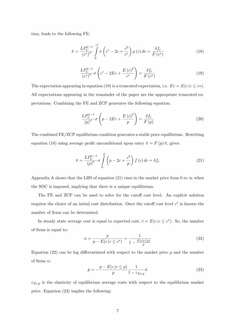
tion, leads to the following FE:
π =LP σ−1
U
(c∗)σ
c∗∫0
σ
(c∗ − 2c+
c2
c∗
)µ (c) dc =
δfeF (c∗)
(18)
LP σ−1U
(c∗)σσ
(c∗ − 2Ec+
E (c)2
c∗
)=
δfeF (c∗)
(19)
The expectation appearing in equation (19) is a truncated expectation, i.e. Ec = E(c |c ≤ c∗).
All expectations appearing in the remainder of the paper are the appropriate truncated ex-
pectations. Combining the FE and ZCP generates the following equation:
LP σ−1U
(p)σσ
(p− 2Ec+
E (c)2
p
)=
δfeF (p)
(20)
The combined FE/ZCP equilibrium condition generates a stable price equilibrium. Rewriting
equation (18) using average profit unconditional upon entry π = F (p) π, gives:
π =LP σ−1
U
(p)σσ
p∫0
(p− 2c+
c2
p
)f (c) dc = δfe (21)
Appendix A shows that the LHS of equation (21) rises in the market price from 0 to∞ when
the SOC is imposed, implying that there is a unique equilibrium.
The FE and ZCP can be used to solve for the cutoff cost level. An explicit solution
requires the choice of an initial cost distribution. Once the cutoff cost level c∗ is known the
number of firms can be determined.
In steady state average cost is equal to expected cost, c = E(c |c ≤ c∗). So, the number
of firms is equal to:
n =p
p− E(c |c ≤ c∗)=
1
1− E(c|c≤p)p
(22)
Equation (22) can be log differentiated with respect to the market price p and the number
of firms n:
p = −p− E(c |c ≤ p)p
11− εEc,p
n (23)
εEc,p is the elasticity of equilibrium average costs with respect to the equilibrium market
price. Equation (23) implies the following:
7

Proposition 2 When the equilibrium average cost varies less than proportionally with mar-
ket price (i.e. it falls slower with a corresponding drop in market price), a lower market
price is coincident with a larger number of firms. Or equivalently, a lower market price
is coincident with more firms when the average markup declines in equilibrium with falling
market prices. When the average cost varies more than proportionally in equilibrium with
lower market prices, a decreasing market price is coincident with less firms.
Proposition 2 follows from equation (22). As the market price is equal to the cutoff cost level,
the relation between the market price and the number of firms depends on the distribution of
costs.4 Intuitively, a lower market price can either be caused by more firms in the market or
by more efficient firms in the market. When average costs respond less than proportionally
to the market price, a lower market price is caused by more firms in the market. When
average costs respond more than proportionally to the market price, a lower market price
is caused by more efficient firms in the market. In this situation a lower market price can
go along with less firms, because the least efficient firms are squeezed out of the market. A
related result can be derived on the effect of market size L on the number of firms.
Proposition 3 The number of firms rises in the size of the market L when equilibrium
average costs decline less than proportionally with equilibrium market price.
The combination of Propositions 1, 2 and 3 leads to the following corollaries about industrial
market structure and market size.
Corollary 1 The mix of price and concentration depends on the distribution of firm costs
(from Proposition 1). While larger markets imply lower prices, larger markets will only have
both more firms and lower prices as long as the equilibrium average cost varies less than
proportionally with equilibrium market price (equation 23). Larger markets will have more
concentration but also lower prices as long as the equilibrium average cost varies more than
proportionally with market price (again as defined in equation 23).
Corollary 2 The relationship of markups to market size also depends on cost heterogeneity.
Larger markets imply both larger markups and greater concentration when the equilibrium4With a Pareto distribution, the truncated mean is linear in the truncation point. Therefore, the number
of firms will be fixed. Simulations show that with a lognormal distribution sensible results can be generatedwith a reasonable number of firms. Moreover, with a lognormal distribution the number of firms declines inthe market price.
8

average cost varies more than proportionally with market price (as defined in equation 23),
and otherwise they imply lower markups and less concentration if equilibrium average cost
varies less than proportionally with market price. From Proposition 1, the latter case is more
likely to hold in industries with lower cost heterogeneity (linked to the technical distribution
of possible costs for a firm).
From Corollary 2, a systematic variation between market size, markups, and concentration
(for example in cross-country comparisons or markups and concentration) can be taken as
an indirect indicator of cost heterogeneity.
The combined FE/ZCP in equation (21) can be totally differentiated towards p and L:
dp
dL= −L
p
p∫0
(p−c)2p f (c) dc
p∫0
((σ + 1) c− (σ − 1) p) f (c) dc< 0 (24)
The denominator is positive by the SOC in equation (7). Equation (24) shows that a larger
market leads to a lower market price. From Proposition 2 it is known that the number of
firms rises in the equilibrium market price when the decline in equilibrium average cost is
less than proportional to a decline in the equilibrium market price, which implies Proposition
2. Intuitively, a larger market can be served in two ways: through more firms or through
an increase in the sales per firm. Depending on the distribution of costs one or the other
dominates.5 The number of firms can increase with a larger market, but the number of firms
can also decrease with a larger market, when enough of the least efficient firms are squeezed
out of the market. This result contrasts with the monopolistic competition model of Melitz,
where the number of firms is linear in market size and the increase in market size is served
through a proportional increase in the number of firms. Here, concentration is an indicator
of underlying heterogeneity, as is price.
3 International Trade without Free Entry: the Short Run
We next introduce international trade between two countries s, r = H, F with markets
effectively segmented by trading costs. The countries are symmetric in size and technology5With a Pareto distribution the number of firms is fixed, so the increase in sales as a result of the larger
market is fully realized through more sales per firm. With a lognormal distribution, also the number of firmschanges considerably.
9
sets. In particular we now introduce iceberg trade costs τ in the Cournot sectors, meaning
that marginal cost for production and delivery is increased at the rate τ relative to production
and delivery for the domestic market. There are no fixed or beachhead trade costs, and the
trading costs preclude return exports. We do not have free entry (we return to this in the
next section) though existing firms can exit. This can be seen as a short-run or free-exit
case. We focus on the impact of increased globalization (i.e. falling trade costs). Consistent
with the empirical literature (Tybout 2001), increased globalization through falling trade
costs means that average markups from domestic sales decline and average markups from
exporting sales rise with falling trade costs.
Under our assumptions about trade costs, the equilibrium market price in the represen-
tative Cournot sector becomes:
ps =σns
σns − 1cs (25)
with cs = 1nr
[nds∑i=1
cids +nxs∑i=1
τcixs
]and ns = nds + nxs. In equation (25), there is a direct
effect of trade liberalization on the market price: exporting firms have lower costs and
therefore average costs decline. And there is an indirect effect, because firms producing for
the domestic market can disappear and exporting firms can appear on the market. It can be
shown that this indirect effect is 0 at the margin (see appendix B). Therefore, the relative
change in the market price is equal to:
Ps =
nxs∑i=1
τcis
nds∑i=1
cis +nxs∑i=1
τcis
τ (26)
Variables with a hat denote relative changes, x = dxx . The elasticity of the market price with
respect to trade costs, εp,τ , is between 0 and 1:
εp,τ =
nxs∑i=1
τcis
nds∑i=1
cis +nxs∑i=1
τcis
(27)
From equations (26) and (27) we make the following proposition:
Proposition 4 With a decline in trade cost τ , the market price also declines.
Equation (26) shows that a decline of trade costs τ drives down the market price. The
10
domestic cutoff marginal cost is equal to the market price, so it also declines.
Several other Propositions can be made on the effect of trade liberalization.
Proposition 5 Some of the least productive firms are squeezed out of the market with a
decline in trade cost τ .
How many firms are squeezed out of the market depends on the price distribution of the
firms, i.e. it depends on how far the highest cost firms are from the old market price.
Proposition 6 More of the remaining firms export with a decline in trade cost τ .
More firms can enter the export market, as the exporting cutoff marginal cost rises when τ
declines:
c∗xr =Psτ
(28)
c∗xr = Ps − τ = − (1− εp,τ ) τ (29)
Proposition 7 (Average) markups from domestic sales decline and (Average) markups from
exporting sales rise with a decline in trade cost τ .
Markups of all domestic sales decline, as the costs of the firms remain equal, whereas the
market price declines. Markups of the exporting firms rise with trade liberalization, as the
effect of the declining trade costs dominates the effect of the decrease in market price in the
exporting market. Using the letter m to indicate markup, the following can be derived:
mixs =Prτcis
(30)
mixs = Pr − τ = (εp,τ − 1) τ (31)
The effect on average domestic and exporting markups can be calculated as well. The
markups of firms are weighted by market shares in calculating average markups, so as to
give more weight to larger firms6:
mids =nds∑i=1
pscisθids =
nds∑i=1
σps − ciscis
(32)
mixs =nxs∑i=1
prτcis
θixs =nxs∑i=1
σpr − τcisτcis
(33)
6Implicitly it is assumed that the probability of firms to be in the market is equal for all marginal costs,i.e. that the distribution of costs is uniform.
11
Relative changes of the average exporting and domestic markups are equal to:
mids =
nds∑i=1
pscis
nds∑i=1
pscisθids
εp,τ τ (34)
mixs = −
nds∑i=1
prτcis
nds∑i=1
prτcis
θixs
(1− εp,τ ) τ (35)
So, average markups from domestic sales decline and average markups from exporting sales
rise.7 Declining markups in the domestic market fit well with empirical findings reported in
Tybout (2001) from developing countries. Various studies find that more import competition
goes along with declining markups.
As in almost any model of international trade (for example Armington) firms increase
their market share on the exporting market and their market share is reduced in domestic
markets. But the relative gain and loss of exporters and domestic producers displays an
interesting pattern:
Proposition 8 Large low cost firms lose less market share on the domestic market than
small high cost firms and small high cost exporting firms gain more market share on the
export market than large low cost firms
Proposition 8 follows from totally differentiating the expressions for market shares:
dθids = σcidspεp,τ τ (36)
dθixs = σcixrp
(εp,τ − 1) τ (37)
Therefore small firms lose relatively more market share on the domestic market and small
firms gain relatively more market share on the exporting market than large firms. So, more
efficient big firms do not gain more from improved market access abroad than less efficient
small firms. Essentially, big firms already have a strong position in an exporting market, so
they cannot grow as much as a result of trade liberalization as small firms.8
7Indirect effects because domestic producing firms disappear from the market and exporting firms enterthe market are 0, because the averages are weighted by market shares and market shares are zero for enteringand exiting firms.
8This set of results, related in particular to Proposition 8, has interesting political economy implications
12
Consider next the welfare effect of trade liberalization. This is complicated by the fact
that income is endogenous as it depends on profit income in the imperfect competition sector.
With free entry profit income is driven to zero, but in the no free entry case profit income is
non-zero and varies.
Welfare in country s is equal to utility in that country:
Ws = Us =IsPUs
=Ls + Πs
PUs(38)
Πs is total profit income in the economy. Elaborating upon this equation (see appendix B)
assuming that both countries are equal, one arrives at the following expression:
W =L (Qp+ pσ)pσ +Qc
1PU
(39)
c are the market share weighted average costs, c =nd∑i=1ciθid +
nx∑i=1τciθix. Log-linearizing
welfare towards trade costs τ from equation (39) and treating the price and the market share
weighted average costs as endogenous, one finds (derivation in appendix B):
W =[
σpσ
Qp+ pσ− σpσ
pσ +Qc
]p− Q
pσ +Qcdc (40)
The first term in (40) is the welfare gain through a decline in price. As expected the gain for
the consumer from lower prices outweighs the loss of a lower profit income with lower prices.
The second term measures the possible gain from trade liberalization of lower costs leading
to a higher profit income. Elaborating on the cost effect, dc, one gets:
W = −[
σpσ
Qp+ pσ− σpσ
pσ +Qc
]p
− Q
pσ +Qc
[nd∑i=1
ciθidθid +nx∑i=1
τciθixθix +nx∑i=1
τciθixτ
](41)
beyond the scope of this paper. As trade liberalization progresses, the dominant domestic firms gain relativedomestic position (known as ”standing” in the antidumping and trade safeguards literature). Assuming thatlobbying efficiency is a function of industry concentration, increased concentration of firms with standing (i.e.the domestic industry) may increase their ability to organize and seek protection or relief against furtherdrops in trade costs and foreign competition.
13
W = −[
σpσ
Qp+ pσ− σpσ
pσ +Qc
]εp,τ τ
− Q
pσ +Qc
[nd∑i=1
σc2i
pεp,τ −
nx∑i=1
στ2c2
i
p(1− εp,τ ) +
nx∑i=1
τciθix
]τ (42)
Equation (41) and (42) can be interpreted as follows. In both equations is the first term
on the RHS again the welfare gain from a lower market price. The second term on the
RHS measures the effect on profit income through changed costs. In both (41) and (42) the
first term between the second brackets measures the gain from the declining market share of
domestic producing firms. The second term between the second brackets measures the loss
from the rising market share of exporting firms. The third term measures the welfare gain
from lower trade costs with trade liberalization.
Proposition 9 Like in Brander and Krugman (1983) the welfare effect of trade liberaliza-
tion can be negative at first when the tariff is reduced from a prohibitive level, due to the
increased costs of cross-hauling associated with the first units traded. However, unlike Bran-
der and Krugman, the welfare effect can also be positive when the tariff is reduced from a
prohibitive level.
Unlike in the model of Brander and Krugman (1983) the welfare effect of trade liberalization
when the tariff is reduced from a prohibitive level is ambiguous. It depends on the cost
structure of firms whether the welfare effect is positive or negative. It can be shown under
what condition the welfare effect is negative in general, but this condition is cumbersome
and does not lend itself to any interpretation. (See footnote 9 below for proof by example).9
The ambiguity vanishes for low trade costs.
Proposition 10 The welfare effect of trade liberalization is unambiguously positive when
the tariff is negligible or small, like in Brander and Krugman (1983)9As proof of ambiguity, we can offer two examples to show that the welfare effect can go both ways. First
an example of a negative welfare effect from trade liberalization. Suppose there are two identical countrieswith each three firms. They have marginal costs of 1, 1 and 2. The autarky market price will be 2. Theiceberg trade costs are equal to 2. This implies that 2 firms can export, but with a market share of 0.Substitution elasticity σ is equal to 1. Equation (42) can be applied to show that a marginal reduction of thetariff decreases welfare with 1
2Q
1+Q. An example where the welfare effect is positive is the following. Again
there are two identical countries with each three firms. Marginal costs are 1, 2 and 3. The autarky marketprice is 3. Iceberg trade costs are 3. So, only one firm can export. Furthermore, the substitution elasticity σis 1, so utility is Cobb-Douglas. There are two sectors in the economy and the Cournot sector has CES-weight(Cobb-Douglas parameter) α. When the tariff is reduced from the prohibitive level, the welfare effect fromequation (42) is equal to (1− α) 5
9− 4
9So, when the Cournot sector is small enough (α < 1/5), the welfare
effect of trade liberalization is positive.
14
Proposition 10 follows immediately from equation (42). When the tariff is equal to 1, the
first two terms between brackets in equation (42) are equal. So, only negative terms are left
and therefore the welfare effect from trade liberalization is positive. Brander and Krugman
(1983) only show that the welfare effect is positive when the tariff is negligible. In the present
heterogeneous productivity model one can say more on when the welfare effect is positive.
Elaborating upon equation (42), the following expression can be derived for the welfare effect
of trade liberalization (see appendix B):
W = −[
σpσ
Qp+ pσ− σpσ
pσ +Qc
]p
− Q
pσ +Qc
σn
p2 (σn− 1)
nx∑i=1
τci [nµc (µc + p− 2τci) + (n− 1)V ar (ci)] τ (43)
In equation (43) µc and V ar (ci) are respectively the mean and variance of the marginal costs
of domestic and exporting firms,
µc =1n
[nd∑i=1
ci +nx∑i=1
τci
](44)
V ar (ci) =1
n− 1
(nd∑i=1
c2i +
nx∑i=1
τ2c2i − nµ2
c
). (45)
Note that the summation in equation (43) is over all the terms between brackets. It can also
be shown that the welfare effect is positive when the following condition is satisfied:
V ar (ci)µ2c
≥ n
(σn− 1) (n− 1)(46)
From equation (43) and (46) the following statements can be made:
Proposition 11 The welfare effect of trade liberalization is positive when the exporting firms
are efficient relative to average market costs. In particular, the welfare effect is unambigu-
ously positive when all exporting firms have marginal costs inclusive of trade costs lower than
the average of market price and average costs.
Proposition 1 The welfare effect of trade liberalization is positive when the coefficient of
variation of the cost distribution is larger than the square root of n(σn−1)(n−1) .
15
Proposition 11 follows from equation (43). When µc + p is larger than 2τci all terms in
equation (43) will be negative and hence the welfare effect of trade liberalization will be
positive. Intuitively, when the exporting firms are productive, their gain in market share at
the expense of domestic producing firms represents a welfare gain. More productive firms
replace less productive firms. But when the exporting firms’ marginal costs inclusive of trade
costs are larger than the marginal costs of the domestic producing firms, the shift in market
share towards exporting firms can represent a loss. In some cases this loss can be larger than
the welfare gain due to lower prices and lower trade costs, as shown by the example above.
Proposition 1 follows from (46). It can be interpreted as follows. When the variance
of firms’ costs is large relative to average firms’ costs, the fraction of relatively inefficient
exporting firms will be small. So, the welfare loss from an increasing market share of relatively
inefficient exporting firms will be smaller than the welfare gain from a decreasing market
share of domestic producing inefficient firms. The next section shows that the welfare effect
from trade liberalization is unambiguously positive with free entry.
4 International Trade with Free Entry: the Long Run
In the free entry case, the welfare effect of trade liberalization depends entirely on the effect
of liberalization on the market price as profit income remains zero. Showing that trade
liberalization leads to a lower market price is sufficient to show that liberalization raises
welfare. In this section we focus on market conditions with falling trade costs based on the
combined ZCP and FE conditions. Trade liberalization does indeed lead to a lower market
price and thus to higher welfare.
Firms can make profits from domestic and exporting sales, if they are productive enough
to export. Average profit is defined as:
πs = πds +F (c∗xs)F(c∗ds) πxs (47)
πds and πxsare the expected profits from respectively domestic and exporting sales, condi-
16

tional upon entry. There are two ZCP for domestic and exporting sales:
c∗ds = ps (48)
c∗xs =prτ
(49)
Elaborating on expected profits as in the closed economy case, generates the following equi-
librium equations deriving from the ZCP and FE:
δfe =LsP
σ−1Us
ps
ps∫0
σ
(ps − 2c+
c2
ps
)f (c) dc+
LrPσ−1Ur
pσr
pr∫0
σ
(pr − 2c+
c2
pr
)f (c) dc (50)
δfe
F(c∗ds) =
LSPσ−1Us
psσ
[ps − 2Ecds +
E (cds)2
ps
]
+F(prτ
)F (ps)
(LrP
σ−1Ur
pσrσ
[pr − 2τEcxs + τ2E (cxs)
2
pr
]) (51)
To determine the impact of trade costs on the market price, one can totally differentiate the
free entry condition in equation (50) towards the cutoff cost level (which equals the market
price) and trade costs. Both the impact of sectoral trade liberalization and trade liberal-
ization in all Cournot sectors can be addressed. The effect of sectoral trade liberalization
on the market price is larger. Totally differentiating towards p and τ one finds the follow-
ing expressions for the effect on market price of sectoral and economywide liberalization
respectively(derivation in appendix C):
p =2
pτ∫0
τc(
1− τcp
)f (c) dc
A+Bτ = εp,τ ,sect,FE τ (52)
p =2
pτ∫0
τc(
1− τcp
)f (c) dc
A+B + Cτ = εp,τ ,nat,FE τ (53)
A =
p∫0
θd (c) ((σ + 1) c− (σ − 1) p) f (c) dc
B =
pτ∫
0
θx (c) ((σ + 1) τc− (σ − 1) p) f (c) dc
C =Qp1−σ
Qp1−σ + 1(πd + πx)
17
εp ,τ ,sect,FE and εp,τ ,nat,FE are the elasticities of the market price with respect to trade costs
in the free entry case with sectoral and nationwide trade liberalization respectively. By the
SOC in equation (7) the denominator in both equations is positive and hence the fraction is
positive as well. This gives rise to the following Proposition:
Proposition 12 Trade liberalization or otherwise falling trade costs τ leads to a lower mar-
ket price and higher welfare in the free entry case.
Welfare rises when the market price of q declines as income is fixed with free entry.10 Hence,
welfare rises in this model as a result of trade liberalization. By Proposition 2 a lower market
price goes along with more or less firms in the market depending on how much average costs
decline when the market price declines. This result can be combined with Proposition 12.
The implication is that the lower market price as a result of trade liberalization can go
along with more but also with less firms in the market, depending on how many of the
least efficient firms are squeezed out of the market. Hence, the conventional insight of the
reciprocal dumping model that trade liberalization leads to lower market prices, because
there are more firms in the market has to be relaxed. Trade liberalization can also lead to
less firms in the market and still decrease market prices, because enough of the least efficient
firms are squeezed out of the market.
The various effects of trade liberalization described in the section on ’no free entry’ can
also be examined in the free entry case. The following effects of trade liberalization are
found:
Proposition 13 The least productive firms get squeezed out of the market with falling trade
costs τ in the free entry case.
Proposition 13 follows from the fact that the cutoff cost level is equal to the market price. A
lower market price implies that the highest cost producers have to leave the market. Next,
the effect on market shares from domestic and exporting sales is calculated.
Proposition 14 Market shares from domestic sales decline and market shares from export-
ing sales rise with declining trade costs τ in the free entry case.
10U = LPU
, U = − Qp1−σ
1+Qp1−σ p
18

Log-differentiating the expressions for market shares, defined implicitly in equations (9) and
using equation (52) gives:
θid =1σ
cip− ci
p =1σ
cip− ci
εp,τ ,FE τ (54)
θix =1σ
τcip− τci
(p− τ) = − 1σ
τcip− τci
(1− εp,τ ,FE) τ (55)
The market share from domestic sales declines for all firms. Therefore, the market share
from exporting sales should rise, either because more firms can export or because the market
share of firms that already exported should rise. The market share of firms that enter the
exporting market is zero. Therefore, the market share of firms already exporting should rise.
Applying this line of reasoning, equation (55) implies that the elasticity of the market price
with respect to iceberg trade costs in equations (52) and (53) is smaller than 1. This result
is useful in the remainder.
Proposition 15 The elasticity of the market price with respect to trade costs is between 0
and 1.
Proposition 15 can immediately be used in the following two Propositions.
Proposition 16 More of the remaining firms are able to export with declining trade cost τ
in the free-entry case.
The exporting cutoff cost level c∗x is equal to pτ . Log-differentiating shows that the exporting
cutoff cost level declines with trade liberalization, implying that more firms can export:
c∗x = p− τ = (εp,τ ,FE − 1) τ (56)
Proposition 17 Markups from domestic sales decline and markups from exporting sales
rise for remaining individual firms with declining trade cost τ in the free entry case.
Markups from domestic sales and exporting sales are equal to pc and p
τc , respectively. Log
differentiating shows that markups from domestic sales decline and markups from exporting
sales rise with trade liberalization:
md = p = εp,τ ,FE τ (57)
mx = p− τ = (εp,τ ,FE − 1) τ (58)
19

While we have clear results for individual firms, the impact on the average across firms
depends on the underlying structure of cost distributions, much like the closed economy case
in Section 2. Basically, market expansion through globalization with falling trade costs τ is
analogous to market expansion in the closed economy case. We summarize this point with
the following proposition:
Proposition 18 While deeper integration through falling trade cost τ implies falling prices,
the impact on average markups across firms and average firm size (whether they rise or fall
on average) depends on the underlying distribution of costs.
Average markups from domestic and exporting sales weighted by market shares are defined,
respectively, as:
md =
p∫0
p
cσp− cp
µ (c) dc =
p∫0
σp− cc
f (c)F (p)
dc (59)
mx =
pτ∫
0
p
τcσp− τcp
µ (c) dc =
pτ∫
0
σp− τcτc
f (c)F( pτ
)dc (60)
Log-differentiating these expressions shows that average markups from domestic sales decline
and average markups from exporting sales rise:
md =σ
τ
p∫0
p
cµ (c) dc− f (p) p
F (p)
p∫0
p− cp
µ (c) dc
εp,τ ,FE (61)
mx =σ
τ
pτ∫
0
p
τcµ (c) dc−
f( pτ
) pτ
F( pτ
)pτ∫
0
p− τcp
µ (c) dc
(εp,τ ,FE − 1) (62)
The terms in f(p)pF (p) represent the increased probability weight of all firms in the market,
when the cutoff point declines as a result of trade liberalization. Basically, as in the closed
or integrated economy case, the effect of trade liberalization (which is somewhat analogous to
market expansion) on average domestic and exporting markups is ambiguous and depends
on the cost distribution of productivities. As in the closed economy case, larger or more
integrated markets imply lower prices, but these lower prices may involve lower or higher
average markups. It depends on the structure of cost heterogeneity.
20

Similarly, as in the case of the closed or integrated economy, we find a similar result for
average firm size (and hence for concentration as well). Average firm size from domestic
sales and exporting sales is defined, respectively, as:
rd =
p∫0
pqd (c)µ (c) dc =P σ−1U L
pσ−1
p∫0
θd (c)µ (c) dc
=P σ−1U L
pσ−1
p∫0
σp− cp
µ (c) dc = P σ−1U Lσ
p∫0
(1
pσ−1− c
pσ
)µ (c) dc (63)
rx =
pτ∫
0
pqx (c)µ (c) dc =P σ−1U L
pσ−1
pτ∫
0
θx (c)µ (c) dc
=P σ−1U L
pσ−1
pτ∫
0
σp− τcp
µ (c) dc = P σ−1U Lσ
pτ∫
0
(1
pσ−1− τc
pσ
)µ (c) dc (64)
Differentiating these expressions towards trade costs generates:
∂rd∂τ
= τP σ−1U L
pσ−1
σ p∫0
(1− θd (c))µ (c) dc− f (p) pF (p)
p∫0
σp− cp
µ (c) dc
εp,τ ,FE (65)
∂rx∂τ
= −P σ−1U L
pσ−1
1τ
pτ∫
0
[(1− θx (c)) (1− εp,τ ) +
σ − 1σ
θx (c)]µ (c) dc
+P σ−1U L
pσ−1
f( pτ
) pτ2
F( pτ
)pτ∫
0
σp− τcpσ
µ (c) dc [1− εp,τ ,FE ] (66)
So, like with average markups, the effect on average domestic and exporting firm sales
depends on the distribution of costs.
5 Asymmetric Countries
So far we have focused on strict symmetry across countries in terms of technology sets and
size. In this section the symmetry assumptions are relaxed. Three sets of results are derived.
First, we show that unilateral liberalization can lead to higher prices in the liberalizing
21
country in the long run. Second, the impact of country size and distance on the probability
of zero trade and on exporting unit values is derived. Third, we present the Ricardian model
with productivity differences as a nested model of the present framework.
The setup in this section is as follows. There are two countries s, r = H, F . The
countries display differences in country size, in trade costs and in their technology sets (cost
distributions). Productivity differences are modeled by a different lower frontier for the
marginal cost distribution, c¯s6=c
¯r. The combined FE/ZCP conditions in both countries
become:
δfe =LsP
σ−1Us
pσs
ps∫c¯s
σ
(ps − 2c+
c2
ps
)fs (c) dc
+LrP
σ−1Ur
pσr
prτsr∫
c¯s
σ
(pr − 2τ src+
τ2src
2
pr
)fs (c) dc (67)
δfe =LrP
σ−1Ur
pσr
pr∫c¯r
σ
(pr − 2c+
c2
pr
)fr (c) dc
+LsP
σ−1Us
pσs
psτrs∫
c¯r
σ
(pr − 2τ rsc+
τ2rsc
2
ps
)fr (c) dc (68)
5.1 asymmetries in trade costs
Unilateral liberalization can be studied using the above two equations. Assuming that the
two countries are equal in all respects except their trade costs, one can log-linearize the above
system of equations towards market prices ps, pr and trade costs τ sr, τ rs. Appendix D shows
that this leads to the following result:
pr =2σ
(qsqrdcdsdcxτr τ rs − dcxrdcxτsτ sr
)dcdsdcdr − dcxsdcxr
(69)
ps =2σ
(qrqsdcdsdcxτsτ sr − dcxsdcxτr τ rs
)dcdsdcdr − dcxsdcxr
(70)
dcds, dcdr, dcxs, dcxr, dcxτs and dcxτr are respectively the marginal effects on expected profit
from domestic and exporting price changes and from trade liberalization in country s and r,
22
defined as follows:
dcds =
ps∫0
θds ((σ + 1) c− (σ − 1) ps) f (c) dc (71)
dcxs =
psτsr∫0
θxs ((σ + 1) c− (σ − 1) pr) f (c) dc (72)
dcxτs =
prτsr∫0
θxs (c) τ srcf (c) dc (73)
The variables in r are defined accordingly. The marginal effects from domestic price changes
on expected profit dcds and dcdr are larger than the marginal effects from exporting prices
on expected profit dcxs and dcxr, because the domestic market shares θd are larger than
the exporting market shares θx and the integration frontier is larger for the domestic cost
variables than for the exporting cost variables.
Equation (26) shows that in the short run unilateral liberalization leads to a lower market
price in the importing country. Equations (69) and (70) show that unilateral liberalization
in country s , i.e. a negative τ rs, decreases the market price in the exporting country s and
increases the market price in the importing country r in the long run. This gives rise to the
following Proposition:
Proposition 19 Unilateral liberalization causes a decreasing market price in the liberalizing
(importing) country in the short run. In the long run, however, the market price in the
importing country increases and the market price in the exporting country decreases. Hence,
the welfare effect of unilateral liberalization is negative in the importing country and positive
in the exporting country.
The short-run effect of unilateral liberalization is as one would expect. The long-run impact is
due to industrial delocation effects.11 Due to unilateral liberalization in country s, expected
profit rises in country r. Therefore, there will be more entry in country r. At the same time,
the decreasing market price in country s reduces entry in that country. The effect of this
entry and exit is that the market price in the exporting country s declines and the market
price in the importing country r rises.12
11With a different model, but also characterized by cost heterogeneity, Melitz and Ottaviano (2008) obtaina similar result.
12Mathematically, the reason for the declining market price in the exporting country s and the rising market
23

5.2 asymmetric size, distance, and zero trade flows
We next focus on the impact of distance and importer country size on the probability of
zero trade and on export prices. We concentrate on country r as the importer country.
First consider the effect of a change in distance. We take as proxy a change in trade costs.
Equations (69) and (70) show the effect of lower trade costs on market prices. Equalizing
the change in trade costs, i.e. τ rs = τ sr = τ , one finds:
pr =2σ
qsqrdcdsdcxτr − dcxrdcxτsdcdsdcdr − dcxsdcxr
τ = εpr τ ,UC τ (74)
ps =2σ
qrqsdcdrdcxτs − dcxsdcxτrdcdsdcdr − dcxsdcxr
τ = εps τ ,UC τ (75)
Unless country sizes differ a lot leading to strong delocation effects, market prices decline
with lower trade costs in the importing country r. Using the same reasoning as in the equal
country case, one can prove that the elasticity of price wrt trade costs, εpr τ ,UC , has to be
between 0 and 1. Market shares of domestic producers in country r and exporters from
country s can be log differentiated to get:
θidr =1σ
cirpr − cir
pr =1σ
cirpr − cir
εpr τ ,UC τ (76)
θixs =1σ
τcispr − τcis
(pr − τ) = − 1σ
τcispr − τcis
(1− εpr τ ,UC) τ (77)
When distance becomes smaller, the market price in country r, pr, declines (if there are no
strong delocation effects). As a result the domestic market shares in the importing country,
θidr decline. Hence, the θixs have to rise to get a total market share of 1 and therefore
0 < εpr τ ,UC < 1. This implies that pr/τ will decline, as the denominator τ declines at a
larger rate than the numerator pr. pr/τ is both the export price and the cutoff cost value
for exports from country s to country r. When the cutoff cost value of exports declines,
the probability of zero trade rises. It becomes more likely that no firm is able to export
price in the importing country r is the following: the marginal effect on expected profit of a changing domesticprice, as represented by cdr and cds, is larger than the effect on expected profit of a changing price in theexport market, represented by cxr and cxs. Therefore, when the expected profit from exports in country srise due to unilateral liberalization in country r, the FE can be restored by decreasing prices in the exportmarket r and/or in the domestic market s. The prices in the two markets should go in opposite directions,however, because the FE in foreign should also be satisfied. Because the marginal effect of domestic pricechanges is larger, the domestic price (in s) has to decrease and the exporting price (in r) has to rise. Withdecreasing export prices (in r) and rising domestic prices (in s), the FE’s could never be satisfied.
24

profitably. Therefore, we have the following result:
Proposition 20 A lower distance between trading partners leads to both a lower probability
of zero trade flows and a lower fob export price.
Consider next the effect of importing country size on the probability of zero trade flows
and export price. The combined FE/ZCP equations, (68) and (67), are log differentiated
wrt pr, ps and Lr, leading to13:
pr = − dcdsπdr − dcrxπsx(dcdrdcds − dcrxdcsx) qr
Lr (78)
ps = − dcsxπdr − dcdrπsx(dcdrdcds − dcrxdcsx) qs
Lr (79)
dcdr, dcxr, dcds and dcxs are respectively the marginal effects on expected profit from domestic
and exporting price changes in country r and country s, as defined in equations (71) and
(72) for country s. As the effect of domestic price changes on expected profit are larger,
because market shares in the domestic market are larger, the denominator in both equations
(78) and (79) is positive. When productivity differences between the two countries are not
too large, expected profits from domestic sales of producers in country r, πdr are larger than
expected profits from exporting sales of exporters from country s, πsx. This implies that
the numerator is also positive. Hence, the market price in country r decreases in its market
size. The fob price of exporters from country s, pr/τ , also decreases. Therefore, we have the
following result:
Proposition 21 A larger market size of the importing country leads to a higher probability
of zero trade flows and lower fob export prices.
Baldwin and Harrigan (2007) compare different models of international trade on their
predictions of the effect of distance and importing country size on the probability of zero trade
flows and fob prices. From table 1 in their paper it is clear that the Cournot model in this
paper generates the same predictions as the Melitz and Ottaviano (2008) model in this regard.
The predictions are different from the model proposed by Baldwin and Harrigan (2007),
which seems to align with the empirical findings presented in their paper. However, whereas13Derivation available upon request. The derivation is similar to the log differentiation wrt pr, ps and τ
discussed in appendix D.
25

the model of Baldwin and Harrigan (2007) contains product differentiation and quality
differences, the oligopoly model in this paper describes a setting with homogeneous products.
Therefore, the predictions from this model should be tested with data from homogeneous
goods sectors and not with a dataset of all sectors as Baldwin and Harrigan (2007) do.
Intuitively, the different predictions can be clearly explained from the different modeling
setups. Baldwin and Harrigan (2007) adapt the Melitz firm heterogeneity model to allow
for quality differences. More productive firms charge higher instead of lower prices, because
they sell higher quality products involving also higher marginal costs. The probability of zero
trade flows rises with distance in our model and in Baldwin and Harrigan (2007). A larger
distance makes it in both models more likely that trade costs are too high and that no firm
is productive enough to sell profitably in the export market. The probability of zero trade
flows rises in importing country size in our model and declines in importing country size in
Baldwin and Harrigan (2007). The intuition in our model is that a larger market leads to
tougher competition, more entry of firms and lower prices. Henceforth, it becomes harder
to export to that market. The model of Baldwin and Harrigan (2007) features fixed export
costs. In a larger market it is easier to earn these fixed costs back and therefore also the less
productive firms with lower quality and lower price can sell in the market profitably.14
A larger distance leads to higher fob export prices in Baldwin and Harrigan (2007) and
lower export prices in our model. In both models a larger distance makes it harder to export
and therefore only more productive firms can export. In our model with homogeneous goods
more productive firms charge lower prices, whereas in Baldwin and Harrigan (2007) they
charge higher prices, because the quality of the good is larger. Finally, the export price
declines in both models in the importing country size. The reason is different, however.
In our model prices are lower in a larger market due to intenser competition and for given
trade costs this leads to lower export prices as well. In Baldwin and Harrigan (2007)
it is easier to earn back the fixed export costs in a larger market. Therefore, also lower
quality, lower price exporters can sell profitably and the average export price will be lower.
It could be an interesting exercise to see if the predictions of Baldwin and Harrigan (2007)
on the probability of trade zeros and export zeros carry through in a sample of sectors with14A larger market also implies a lower price index and therefore less sales for an individual firm, making it
more difficult to sell profitably in the export market. Apparently the direct effect of market size dominates.An effect of market size on profit margins is absent in the model of Baldwin and Harrigan (2007) , becausethey work with CES and thus fixed markups.
26

homogeneous goods or if our model of oligopoly predicts better.
5.3 technology asymmetries
With technological asymmetries, the Ricardian comparative advantage can be treated as a
nested case of the present model. Comparative advantage is introduced in this case as follows.
There are two types of sectors, country s has a comparative advantage in the A sectors and
country r has a comparative advantage in the B sectors. Comparative advantage is modeled
by the integration frontiers of the initial distribution of productivities. As only the lower
integration frontiers c¯
appears in the relevant ZCP and FE equations, attention can be
restricted to these. The following assumptions are made to define comparative advantage:
c¯sA
< c¯rA
(80)
c¯sB
> c¯rB
(81)
c¯sA
is the lower integration frontier in country s in the A sectors, i.e. in the sectors in which
country s has a comparative advantage. To show that Ricardian comparative advantage is
a nested case of the model, the distribution of productivities within a country is squeezed,
i.e. the heterogeneity of firms is reduced. The productivity differences between countries
remain. When the within country distribution of productivities collapses to a single point,
the model converges either to a Ricardian model with perfect competition or a Brander and
Krugman (1983) Cournot model with specialization, depending on whether the sunk entry
costs disappear or not.
Before the distribution of productivities is narrowed, the following relations between the
lower integration frontiers, market prices and trade costs apply:
c¯sA
< c¯rA
< prA/τ < prA (82)
c¯sA
< c¯rA
< psA/τ < psA (83)
The focus in the discussion is on sector A, because sector B is just its mirror image with
a comparative advantage for country r. Equation (82) ensures that at least some firms in
country s can export in their comparative advantage sector A and that at least some firms
27

in country r can produce for the domestic market. Equation (83) guarantees that some firms
in country r can also export in their comparative disadvantage market A and that firms in
country s can sell in their domestic market in their comparative advantage sector A. Hence,
there is two-way trade in sector A.
Next, suppose that the distribution of productivities becomes more homogenous. This
can be seen as a narrowing of the distribution of productivities. The lower integration
frontier moves up and the upper integration frontier moves down. However, only the lower
integration frontier appears in the combined ZCP/FE condition, so mathematically a more
homogenous productivity distribution comes down to an increase in the lowest cost.
Uncertainty about productivity is a barrier to entry for firms. The sunk entry costs are
dependent on uncertainty about the prospective productivity. Firms have to incur research
costs to get rid of the uncertainty about their productivity. This interpretation of the sunk
entry costs implies that a squeezing of the productivity distribution decreases the sunk
entry costs. The combined ZCP/FEs in a S sector are given in equations (67) and (68) (with
symmetric trade costs). Log differentiating these expressions towards market prices, the lower
integration frontiers and the sunk entry costs shows what happens when the distributions of
productivities become more homogenous:
qs
ps∫c¯s
θds ((σ + 1) c− (σ − 1) ps) fsdcps + qr
prτ∫
c¯s
θxs ((σ + 1) τc− (σ − 1) pr) fsdcpr
−σqsc¯s(ps − 2c
¯s+
c¯
2s
ps
)f (c
¯s) cs + qrc¯s
(pr − 2τc
¯s+τ2c
¯2s
pr
)f (c
¯s) cs = δfefe (84)
qr
pr∫c¯r
θdr ((σ + 1) c− (σ − 1) pr) frdcpr + qs
prτ∫
c¯r
θxr ((σ + 1) τc− (σ − 1) ps) frdcps
−σqrc¯r(pr − 2c
¯r+
c¯
2r
pr
)f (c
¯r) cr + qsc¯r
(ps − 2τc
¯r+τ2c
¯2r
ps
)f (c
¯r) cr = δfefe (85)
The effect of squeezing the distribution of productivities on market prices depends on the
size of the change in the sunk entry cost fe. When this change is small, the market prices
will have to rise to keep on satisfying the free entry condition.
Suppose that the distribution of productivities becomes concentrated in one point. Then
two questions remain. First, does the model converge to a Ricardian comparative advantage
28
model with perfect competition or a Brander and Krugman Cournot model? Second, will
there be full specialization across countries? To address the first question, where the model
converges to depends on what happens with sunk entry costs. When some sunk entry costs
remain, because uncertainty about productivity is not the only source of the sunk costs, the
model remains Cournot. The market price becomes higher than marginal costs to cover the
sunk entry costs and the number of firms is limited. When uncertainty is the only source of
sunk costs and so when there are no sunk costs left when the distribution of productivities
collapses to a single point, the model converges to a perfect competition Ricardian model.
Marginal cost will be equal to the market price and the number of firms becomes infinite as
is clear from equation (13).15
Proposition 22 When the distribution of productivities becomes concentrated in one point
the model either converges to a Brander & Krugman Cournot model or a Ricardian perfect
competition model depending on the presence of sunk (or fixed) costs. Two-way trade emerges
either from cost heterogeneity or the presence of sunk (or fixed) entry costs.
Whether there will be full specialization depends on the relation between market prices and
marginal cost levels that emerges. There will be full specialization when:
c¯rA
< psA/τ < c¯sA
(86)
crA < prA < τc¯sA
(87)
The model converges either to a Cournot model or a Ricardian perfect competition model
depending on the presence of sunk costs. There is no strict link between the appearance
of full specialization and the type of market competition that emerges. There can be full
specialization with Cournot competition when productivity differences are large enough.
Also, the Ricardian model does not imply full specialization. A country could still produce
for its own market in the Ricardian model in its comparative disadvantage sector when
trade costs are large enough. But two way trade is only possible with Cournot competition.
Moreover, full specialization is more likely in the Ricardian model without fixed costs, because
market prices become equal to marginal costs (inclusive of trade costs) in that case.15It should be noted that there are no wage differences in the present model. Modeling wage differences,
possibly along the line of the Dornbusch-Fischer-Samuelson model of Ricardian trade with a continuum ofgoods and technology asymmetries, constitutes a possible extension of the present model
29

Proposition 23 When the distribution of productivities collapses to a single point, full spe-
cialization is more likely with lower trade costs, a larger cost difference between countries
and the absence of sunk costs.
6 Summary and Conclusions
We have developed a model of trade with endogeneity in key features of market structure
linked to heterogeneous cost structures under Cournot competition. This approach leads to a
set of results familiar from the recent Bertrand and Chamberlinian monopolistic competition
literature with cost heterogeneity. Market prices decline, the least productive firms get
squeezed out of the market and exporting firms gain market share when trade costs fall.
These results hold in cases with and without free entry. Welfare rises in both cases with
trade liberalization, unless the trade barriers decline from a prohibitive level in the short run.
With asymmetric countries, the Brander & Krugman’s (1983) reciprocal dumping model and
the Ricardian comparative advantage model can be nested as special cases. Furthermore,
delocation effects are present in the asymmetric trade cost case: unilateral liberalization leads
in the long run to higher prices in the liberalizing country, because firms delocate to the other
country. Possible extensions of the model are the introduction of wage differences between
the two countries, political economy applications (as domestic industry concentration is
endogenous to the evolution of trade policy), and specifying a distribution of costs enabling
simulations with the model with more countries and more sectors.
The model provides insight into zero trade flows and the pattern of export prices. The
probability of zero trade flows rises with distance and with the size of the importer country,
while fob export prices decrease with distance and with the size of the importer country. The
model also offers insight into cross-country differences in markups, concentration, and prices
across industries controlling for different degrees of openness. In particular, the variation
across industries and countries in markups, concentration, and pricing structures is also a
function of country or market size and the variation in cost heterogeneity across industries.
30
References
Baldwin, Richard and James Harrigan (2007). “Zeros, Quality and Space: Trade
Theory and Trade Evidence.” NBER Working Paper No. 13214
Baldwin, Richard and Frederic Robert-Nicoud(2005). “Trade and Growth with Het-
erogeneous Firms.” Journal of International Economics 74(1): 21-34.
Baldwin, Richard and Daria Taglioni (2007). “Gravity for Dummies and Dummies
for Gravity Equations.” CEPR Discussion Paper No. 5850.
Bernard, Andrew B., Jonathan Eaton, J. Bradford Jensen, and Samuel Kor-
tum (2003). “Plants and Productivity in International Trade.” American Economic Review
93(4): 1268-1290.
Bernard, Andrew B. and J. Bradford Jensen (2004). “Exporting and Productivity
in the USA.” Oxford Review of Economic Policy 20(3).
Brander, James and Paul Krugman (1983). “A ’Reciprocal Dumping’ Model of Inter-
national Trade.”Journal of International Economics 15: 313-321.
Ghironi, F. and Marc J. Melitz(2004). “International Trade and Macroeconomic Dy-
namics with Heterogeneous Firms.” American Economic Review 97(2): 356-361.
Melitz, Marc J. (2003). “The Impact of Trade on Intra-Industry Reallocations and Ag-
gregate Industry Productivity.” Econometrica 71(6): 1695-1725.
Melitz, Marc J. and Gianmarco I.P. Ottaviano (2008), “Market Size, Trade, and
Productivity,” Review of Economic Studies 75(1): 295-316.
Tybout, James R. (2001). “Plant and Firm-Level Evidence on New Trade Theories.” in:
Harrigan J. (ed.), Handbook of International Economics 38, Basil-Blackwell. Also: NBER
Working Paper No. 8414.
Van Long, Ngo and Antoine Soubeyran (1997), “Cost Heterogeneity, Industry Con-
centration and Strategic Trade Policies.” Journal of International Economics 43: 207-220.
31
Appendix A Basic Model
The appendices show how to derive equations from the main text.
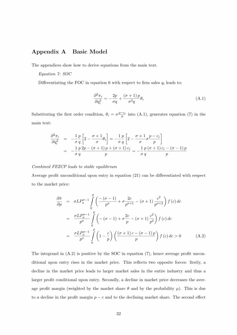
Equation 7: SOC
Differentiating the FOC in equation 6 with respect to firm sales qi leads to:
∂2πi∂q2
i
= − 2pσq
+(σ + 1) pσ2q
θi (A.1)
Substituting the first order condition, θi = σ p−cip into (A.1), generates equation (7) in the
main text:
∂2πi∂q2
i
= − 1σ
p
q
[2− σ + 1
σθi
]= − 1
σ
p
q
[2− σ + 1
σσp− cip
]= − 1
σ
p
q
2p− (σ + 1) p+ (σ + 1) cip
= − 1σ
p
q
(σ + 1) ci − (σ − 1) pp
Combined FEZCP leads to stable equilibrium
Average profit unconditional upon entry in equation (21) can be differentiated with respect
to the market price:
∂π
∂p= σLP σ−1
u
p∫0
(− (σ − 1)
pσ+ σ
2cpσ+1
− (σ + 1)c2
pσ+2
)f (c) dc
=σLP σ−1
u
pσ
p∫0
(− (σ − 1) + σ
2cp− (σ + 1)
c2
p2
)f (c) dc
=σLP σ−1
u
pσ
p∫0
(1− c
p
)((σ + 1) c− (σ − 1) p
p
)f (c) dc > 0 (A.2)
The integrand in (A.2) is positive by the SOC in equation (7), hence average profit uncon-
ditional upon entry rises in the market price. This reflects two opposite forces: firstly, a
decline in the market price leads to larger market sales in the entire industry and thus a
larger profit conditional upon entry. Secondly, a decline in market price decreases the aver-
age profit margin (weighted by the market share θ and by the probability µ). This is due
to a decline in the profit margin p− c and to the declining market share. The second effect
32
dominates the first effect. Hence, the model generates a stable equilibrium market price.
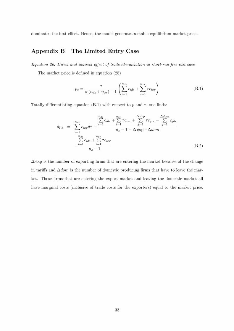
Appendix B The Limited Entry Case
Equation 26: Direct and indirect effect of trade liberalization in short-run free exit case
The market price is defined in equation (25)
ps =σ
σ (nds + nxr)− 1
(nds∑i=1
cids +nxr∑i=1
τcixr
)(B.1)
Totally differentiating equation (B.1) with respect to p and τ , one finds:
dps =nxr∑i=1
cixrdτ +
nds∑i=1
cids +nxr∑i=1
τcixr +∆ exp∑j=1
τcjxr −∆dom∑j=1
cjdr
ns − 1 + ∆ exp−∆dom
−
nds∑i=1
cids +nxr∑i=1
τcixr
ns − 1(B.2)
∆ exp is the number of exporting firms that are entering the market because of the change
in tariffs and ∆dom is the number of domestic producing firms that have to leave the mar-
ket. These firms that are entering the export market and leaving the domestic market all
have marginal costs (inclusive of trade costs for the exporters) equal to the market price.
33
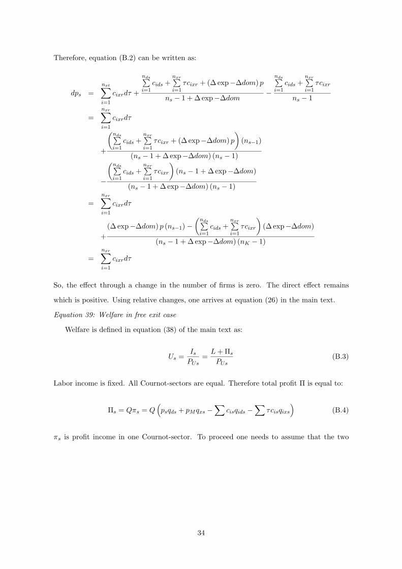
Therefore, equation (B.2) can be written as:
dps =nxt∑i=1
cixrdτ +
nds∑i=1
cids +nxr∑i=1
τcixr + (∆ exp−∆dom) p
ns − 1 + ∆ exp−∆dom−
nds∑i=1
cids +nxr∑i=1
τcixr
ns − 1
=nxr∑i=1
cixrdτ
+
(nds∑i=1
cids +nxr∑i=1
τcixr + (∆ exp−∆dom) p)
(ns−1)
(ns − 1 + ∆ exp−∆dom) (ns − 1)
−
(nds∑i=1
cids +nxr∑i=1
τcixr
)(ns − 1 + ∆ exp−∆dom)
(ns − 1 + ∆ exp−∆dom) (ns − 1)
=nxr∑i=1
cixrdτ
+(∆ exp−∆dom) p (ns−1)−
(nds∑i=1
cids +nxr∑i=1
τcixr
)(∆ exp−∆dom)
(ns − 1 + ∆ exp−∆dom) (nK − 1)
=nxr∑i=1
cixrdτ
So, the effect through a change in the number of firms is zero. The direct effect remains
which is positive. Using relative changes, one arrives at equation (26) in the main text.
Equation 39: Welfare in free exit case
Welfare is defined in equation (38) of the main text as:
Us =IsPUs
=L+ Πs
PUs(B.3)
Labor income is fixed. All Cournot-sectors are equal. Therefore total profit Π is equal to:
Πs = Qπs = Q(psqds + pMqxs −
∑cisqids −
∑τcisqixs
)(B.4)
πs is profit income in one Cournot-sector. To proceed one needs to assume that the two
34

countries are equal. This implies that (B.4) can be rewritten as:
ΠQ
= p (qd + qx)−nd∑i=1
ciqid −nx∑i=1
ciτqix
ΠQ
= pq − qnd∑i=1
ciθid − qnx∑i=1
ciτθix
ΠQ
=IP σ−1
U
pσ−1
p−nd∑i=1
ciθid +nx∑i=1
ciτθix
p
(B.5)
ΠQ
= (L+ Π)P σ−1U
pσ(p− c) (B.6)
The termnd∑i=1
ciθid+nx∑i=1
ciτθix in (B.5) represents the market share weighted average of costs,
c. Therefore,(p−
nd∑i=1
ciθid −nx∑i=1
ciτθix
)is defined as the market share weighted average
profit per unit of sales, π. Solving for L+ Π from (B.6) yields:
ΠQ−Π
P σ−1U
pσ(p− c) = L
P σ−1U
pσ(p− c)
Π
(1−
QP σ−1U
pσ(p− c)
)= QL
P σ−1U
pσ(p− c)
Π =QL
Pσ−1Upσ (p− c)
1− QPσ−1Upσ (p− c)
L+ Π =L
1− QPσ−1U (p−c)pσ
(B.7)
Substituting equation (B.7) into equation (B.3), one finds the following expression for welfare,
equation (39) in the main text:
W =L
1− QPσ−1U (p−c)pσ
1PU
=L
1− Q(p−c)(Qp1−σ+1)pσ
1PU
=L
1− Q(p−c)Qp+pσ
1PU
W =L (Qp+ pσ)pσ +Qc
1PU
(B.8)
Equation 40: Relative Welfare Change in free exit case
Log-differentiating equation (B.8) with respect to trade costs τ , treating the market price p,
the price index PU and average costs c as endogenous generates equation (40) in the main
35

text:
W =Qp+ σpσ
Qp+ pσp− σpσp+Qdc
pσ +Qc− PU
=(Qp+ σpσ
Qp+ pσ− σpσ
pσ +Qc
)p− Q
pσ +Qcdc− Qp1−σ
Qp1−σ + 1p
W =(
σpσ
pσ +Qp− σpσ
pσ +Qc
)p− Q
pσ +Qcdc (B.9)
Equation 43 and 46: Conditions for positive welfare effect of trade liberalization
Starting from equation (B.9), one can elaborate on the term dc. Using equations (9), (36),
(37), dc can be rewritten as follows:
dc =nd∑i=1
cip− cip
cip− ci
εp,τ τ +nx∑i=1
τcip− τcip
τcip− τci
(εp,τ − 1) τ +nx∑i=1
τcip− τcip
τ (B.10)
Using equation (27) one can substitute for the price elasticity in equation (B.10) to get:
dc =nd∑i=1
σc2i
p
nx∑i=1
τci
nd∑i=1
ci +nx∑i=1
τci
τ +nx∑i=1
στ2c2
i
p
nx∑i=1
τci
nd∑i=1
ci +nx∑i=1
τci
τ − 2nx∑i=1
στ2c2
i
pτ +
nx∑i=1
σpτcipτdc
σ
nd∑i=1
c2i
p
nx∑i=1
τci
nd∑i=1
ci +nx∑i=1
τci
τ + σ
nx∑i=1
τ2c2i
p
nx∑i=1
τci
nd∑i=1
ci +nx∑i=1
τci
τ
−σ
(2nx∑i=1
τ2c2i
p−
nx∑i=1
pτcip
) nd∑i=1
ci +nx∑i=1
τci
nd∑i=1
ci +nx∑i=1
τci
τ
dc =1
p
(nd∑i=1
ci +nx∑i=1
τci
)∗[σ
nd∑i=1
c2i
nx∑i=1
τciτ + σ
nx∑i=1
τ2c2i
nx∑i=1
τciτ − σ
(nx
2∑i=1
τ2c2i − p
nx∑i=1
τci
)(nd∑i=1
ci +nx∑i=1
τci
)τ
](B.11)
Next, p = σσn−1
(nd∑i=1
ci +nx∑i=1
τci
), µc = 1
n
(nd∑i=1
ci +nx∑i=1
τci
), also implying that, p = σn
σn−1µc can
be used to rewrite (B.11) as:
dc =σn
p2 (σn− 1)
[(nd∑i=1
c2i +
nx∑i=1
τ2c2i
)nx∑i=1
τciτ −
(2nx∑i=1
τ2c2i − p
nx∑i=1
τci
)nµcτ
](B.12)
36
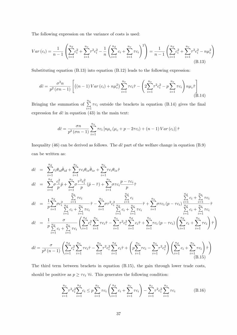
The following expression on the variance of costs is used:
V ar (ci) =1
n− 1
nd∑i=1
c2i +
nx∑i=1
τ2c2i −
1n
(nd∑i=1
ci +nx∑i=1
τci
)2 =
1n− 1
(nd∑i=1
c2i +
nx∑i=1
τ2c2i − nµ2
c
)(B.13)
Substituting equation (B.13) into equation (B.12) leads to the following expression:
dc =σ2n
p2 (σn− 1)
[((n− 1)V ar (ci) + nµ2
c
) nx∑i=1
τciτ −
(2nx∑i=1
τ2c2i − p
nx∑i=1
τci
)nµcτ
](B.14)
Bringing the summation ofnx∑i=1
τci outside the brackets in equation (B.14) gives the final
expression for dc in equation (43) in the main text:
dc =σn
p2 (σn− 1)
nx∑i=1
τci [nµc (µc + p− 2τci) + (n− 1)V ar (ci)] τ
Inequality (46) can be derived as follows. The dc part of the welfare change in equation (B.9)
can be written as:
dc =nd∑i=1
ciθidθid +nx∑i=1
τciθixθix +nx∑i=1
τciθixτ
dc =nd∑i=1
σc2i
pp+
nx∑i=1
στ2c2
i
p(p− τ) +
nx∑i=1
στcip− τcip
τ
dc =1p
nd∑i=1
σc2i
nx∑i=1
τci
nd∑i=1
ci +nx∑i=1
τci
τ −nx∑i=1
στ2c2i
nd∑i=1
ci
nd∑i=1
ci +nx∑i=1
τci
τ +nx∑i=1
στci (p− τci)
nd∑i=1
ci +nx∑i=1
τci
nd∑i=1
ci +nx∑i=1
τci
τ
dc =1p
σnd∑i=1
ci +nx∑i=1
τci
(nd∑i=1
c2i
nx∑i=1
τciτ −nx∑i=1
τ2c2i
nd∑i=1
ciτ +nx∑i=1
τci (p− τci)
(nd∑i=1
ci +nx∑i=1
τci
)τ
)
dc =σ
p2 (n− 1)
(nd∑i=1
c2i
nx∑i=1
τciτ −nx∑i=1
τ2c2i
nd∑i=1
ciτ +
(p
nx∑i=1
τci −nx∑i=1
τ2c2i
)(nd∑i=1
ci +nx∑i=1
τci
)τ
)(B.15)
The third term between brackets in equation (B.15), the gain through lower trade costs,
should be positive as p ≥ τci ∀i. This generates the following condition:
nx∑i=1
τ2c2i
nd∑i=1
ci ≤ pnx∑i=1
τci
(nd∑i=1
ci +nx∑i=1
τci
)−
nx∑i=1
τ2c2i
nx∑i=1
τci (B.16)
37

Substituting the condition in (B.16) into the first two terms of dc in equation (B.15) one can
proceed as follows:
dc ≥
[nd∑i=1
c2i
nx∑i=1
τci − pnx∑i=1
τci
(nd∑i=1
ci +nx∑i=1
τci
)+
nx∑i=1
τ2c2i
nx∑i=1
τci
]τ
dc ≥nx∑i=1
τci
[(nd∑i=1
c2i +
nx∑i=1
τ2c2i
)− p
(nd∑i=1
ci +nx∑i=1
τci
)]τ
dc ≥nx∑i=1
τci[(n− 1)V ar (ci) + nµ2
c − pnµc]τ
dc ≥nx∑i=1
τci [(n− 1)V ar (ci) + nµc (µc − p)] τ
dc ≥nx∑i=1
τci
[(n− 1)V ar (ci) + nµc
(µc −
σn
σn− 1µc
)]τ
dc ≥nx∑i=1
τci
[(n− 1)V ar (ci) +
σn
σn− 1µ2c
]τ (B.17)
So, from the inequality in (B.17) dc is positive whenever V ar(ci)µ2c≥ σn
(n−1)(σn−1) , condition
(46) in the main text.
Appendix C Free Entry Case
Equation 52: Effect of sectoral trade liberalization on market price in free entry case
Assuming equal countries, the combined FE/ZCP condition, equation (50) is given by:
LP σ−1U
pσ
p∫0
σ
(p− 2c+
c2
p
)f (c) dc+
LP σ−1U
pσ
p∫0
σ
(p− 2c+
c2
p
)f (c) dc = δfe (C.1)
Totally differentiating equation (C.1) towards p and τ and considering the effect through the
38
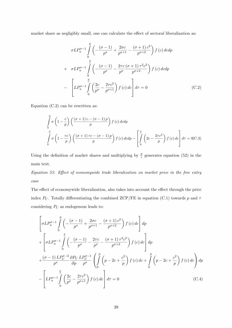
market share as negligibly small, one can calculate the effect of sectoral liberalization as:
σLP σ−1u
p∫0
(−(σ − 1)
pσ+
2σcpσ+1
− (σ + 1) c2
pσ+2
)f (c) dcdp
+ σLP σ−1u
pτ∫
0
(−(σ − 1)
pσ− 2τc
pσ(σ + 1) τ2c2
pσ+2
)f (c) dcdp
−
LP σ−1u
pτ∫0
(2cpσ− 2τc2
pσ+1
)f (c) dc
dτ = 0 (C.2)
Equation (C.2) can be rewritten as:
p∫0
σ
(1− c
p
)((σ + 1) c− (σ − 1) p
p
)f (c) dcdp
pτ∫
0
σ
(1− τc
p
)((σ + 1) τc− (σ − 1) p
p
)f (c) dcdp−
pτ∫0
(2c− 2τc2
p
)f (c) dc
dτ = 0(C.3)
Using the definition of market shares and multiplying by pτ generates equation (52) in the
main text.
Equation 53: Effect of economywide trade liberalization on market price in the free entry
case
The effect of economywide liberalization, also takes into account the effect through the price
index PU . Totally differentiating the combined ZCP/FE in equation (C.1) towards p and τ
considering PU as endogenous leads to:
σLP σ−1u
p∫0
(−(σ − 1)
pσ+
2σcpσ+1
− (σ + 1) c2
pσ+2
)f (c) dc
dp+
σLP σ−1u
pτ∫
0
(−(σ − 1)
pσ− 2τc
pσ− (σ + 1) τ2c2
pσ+2
)f (c) dc
dp+
(σ − 1)LP σ−2U
pσ∂PU∂p
LP σ−1U
pσ
p∫0
(p− 2c+
c2
p
)f (c) dc+
p∫0
(p− 2c+
c2
p
)f (c) dc
dp
−
LP σ−1u
pτ∫0
(2cpσ− 2τc2
pσ+1
)f (c) dc
dτ = 0 (C.4)
39
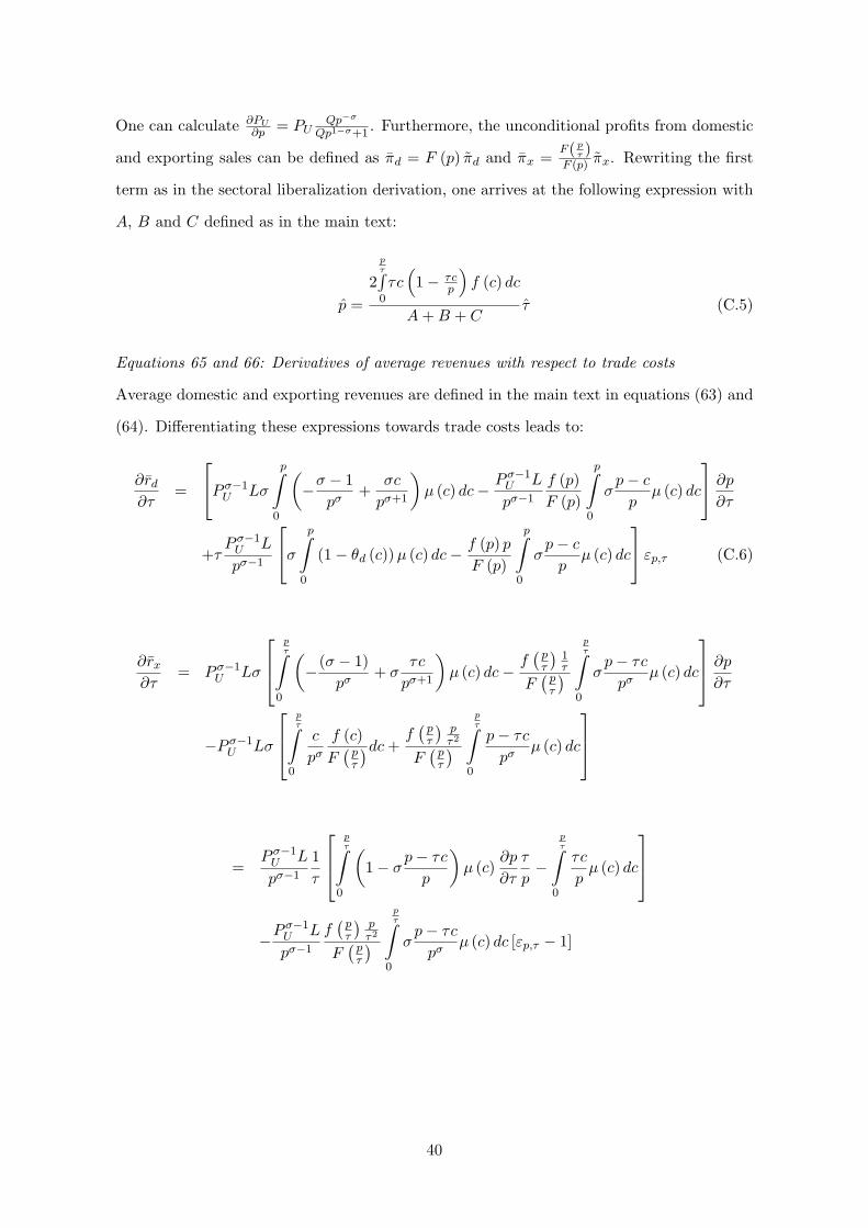
One can calculate ∂PU∂p = PU
Qp−σ
Qp1−σ+1. Furthermore, the unconditional profits from domestic
and exporting sales can be defined as πd = F (p) πd and πx =F( pτ )F (p) πx. Rewriting the first
term as in the sectoral liberalization derivation, one arrives at the following expression with
A, B and C defined as in the main text:
p =2
pτ∫0
τc(
1− τcp
)f (c) dc
A+B + Cτ (C.5)
Equations 65 and 66: Derivatives of average revenues with respect to trade costs
Average domestic and exporting revenues are defined in the main text in equations (63) and
(64). Differentiating these expressions towards trade costs leads to:
∂rd∂τ
=
P σ−1U Lσ
p∫0
(−σ − 1
pσ+
σc
pσ+1
)µ (c) dc−
P σ−1U L
pσ−1
f (p)F (p)
p∫0
σp− cp
µ (c) dc
∂p∂τ
+τP σ−1U L
pσ−1
σ p∫0
(1− θd (c))µ (c) dc− f (p) pF (p)
p∫0
σp− cp
µ (c) dc
εp,τ (C.6)
∂rx∂τ
= P σ−1U Lσ
pτ∫
0
(−(σ − 1)
pσ+ σ
τc
pσ+1
)µ (c) dc−
f( pτ
)1τ
F( pτ
)pτ∫
0
σp− τcpσ
µ (c) dc
∂p∂τ
−P σ−1U Lσ
pτ∫
0
c
pσf (c)F( pτ
)dc+f( pτ
) pτ2
F( pτ
)pτ∫
0
p− τcpσ
µ (c) dc
=P σ−1U L
pσ−1
1τ
pτ∫
0
(1− σp− τc
p
)µ (c)
∂p
∂τ
τ
p−
pτ∫
0
τc
pµ (c) dc
−P σ−1U L
pσ−1
f( pτ
) pτ2
F( pτ
)pτ∫
0
σp− τcpσ
µ (c) dc [εp,τ − 1]
40

= −P σ−1U L
pσ−1
1τ
pτ∫
0
[(1− θx (c)) (1− εp,τ ) +
σ − 1σ
θx (c)]µ (c) dc
−P σ−1U L
pσ−1
f( pτ
) pτ2
F( pτ
)pτ∫
0
σp− τcpσ
µ (c) dc [εp,τ − 1] (C.7)
Appendix D Asymmetric Countries Case
Equations 69 and 70: Effects of unilateral trade liberalization on market prices
The combined FE/ZCP’s in country s and r are given by:
LsPσ−1Us
pσs
ps∫c¯s
(ps − 2c+
c2
ps
)fs (c) dc+
LrPσ−1Ur
pσr
prτsr∫
c¯s
(pr − 2τ src+
τ2src
2
pr
)fs (c) dc = δfe
(D.1)
LrPσ−1Ur
pσr
pr∫c¯r
(pr − 2c+
c2
pr
)fr (c) dc+
LsPσ−1Us
pσs
psτrs∫
c¯r
(ps − 2τ rsc+
τ2rsc
2
ps
)fr (c) dc = δfe
(D.2)
Totally differentiating equation (D.1) towards ps, pr and τ sr gives:
σLsPσ−1Us
pσs
ps∫0
(1− c
ps
)((σ + 1) c− (σ − 1) ps
ps
)f (c) dcdps
+σLrP
σ−1Ur
pσr
prτsr∫0
(1− τ src
pr
)((σ + 1) τ src− (σ − 1) pr
pr
)f (c) dcdpr
−LrP
σ−1Ur
pσr2
prτsr∫0
(c− 2τ src2
pr
)f (c) dcdτ sr = 0 (D.3)
Rewriting equation (D.3) in terms of relative changes and adding the equivalent expression
for the other country, one arrives at:
qs
ps∫0
θds (c) ((σ + 1) c− (σ − 1) ps) f (c) ps
+qr
prτsr∫0
θxs (c) ((σ + 1) τ src− (σ − 1) pr) f (c) dcpr−2qrσ
prτsr∫0
τ srcθxs (c) f (c) dcτ sr = 0 (D.4)
41

qr
pr∫0
θdr (c) ((σ + 1) c− (σ − 1) pr) f (c) pr
+qs
psτrs∫0
θxr (c) ((σ + 1) τ rsc− (σ − 1) ps) f (c) dcpK −2qsσ
psτrs∫0
τ rscθxr (c) f (c) dcτ rs = 0
(D.5)
Defining the marginal effects dcds, dcdr, dcxs, dcxr, dcxτs and dcxτr as in the main text,
equations (D.4) and (D.5) can be solved for ps, pr as a function of τ sr and τ rs, leading to
equations (69) and (70) in the main text.
42