Heuristics-based SPARQL Query Planning

Fuqi Song, Olivier Corby

To cite this version:

Fuqi Song, Olivier Corby. Heuristics-based SPARQL Query Planning. [Research Report] RR-8655, Inria Sophia Antipolis; I3S; INRIA. 2014, pp.17. <hal-01096313>

HAL Id: hal-01096313

https://hal.inria.fr/hal-01096313

Submitted on 17 Dec 2014

HAL is a multi-disciplinary open accessarchive for the deposit and dissemination of sci-entific research documents, whether they are pub-lished or not. The documents may come fromteaching and research institutions in France orabroad, or from public or private research centers.

L’archive ouverte pluridisciplinaire HAL, estdestinee au depot et a la diffusion de documentsscientifiques de niveau recherche, publies ou non,emanant des etablissements d’enseignement et derecherche francais ou etrangers, des laboratoirespublics ou prives.

ISS

N0

24

9-6

39

9IS

RN

INR

IA/R

R--

86

55

--F

R+

EN

G

RESEARCH

REPORT

N° 8655December 2014

Project-Teams Wimmics

Heuristics-based

SPARQL Query Planning

Fuqi Song, Olivier Corby

RESEARCH CENTRE

SOPHIA ANTIPOLIS – MÉDITERRANÉE

2004 route des Lucioles - BP 93

06902 Sophia Antipolis Cedex

Heuristics-based SPARQL Query Planning

Fuqi Song ∗, Olivier Corby †

Équipes-Projets Wimmics

Rapport de recherche n° 8655 — December 2014 — 17 pages

Résumé : La planification de requête joue un rôle essentiel dans l’optimisation de l’exécution desrequêtes SPARQL. Ce rapport présente une méthode de planification basée sur des heuristiquespour optimiser l’exécution de requêtes et une implémentation réalisée dans la plateforme Corese.Dans un premier temps, nous proposons une représentation abstraite des énoncés SPARQL engénéralisant les représentations habituellement utilisées à d’autres énoncés que les simples triplets.Ensuite, nous étendons les heuristiques utilisées habituellement pour estimer le coût des énoncés.Les méthodes proposées sont évaluées sur le benchmark BSBM. Les résultats montrent que lesméthodes proposées optimisent effectivement le temps d’exécution du moteur Corese et montrentégalement certains avantages comparés à Jena et Sesame utilisés en mode mémoire vive.

Mots-clés : SPARQL, query planning, query optimization, heuristics, Corese

∗ Inria, I3S, fuqi.song@inria.fr† Inria, I3S, olivier.corby@inria.fr

Heuristics-based SPARQL Query Planning

Abstract: SPARQL query planning, as an essential task of query optimizer in SPARQL queryengine, plays a significant role in improving query execution performance. Based on Coresequery engine, this report presents a heuristic-based approach for performing query planning andoptimization. First, this report generalizes SPARQL query statement representation by takingother expressions into account, aiming at overcoming the limitations of only using basic querytriple patterns. Second, this report extends the heuristics for estimating the cost of query triplepattern. The proposed query planning methods are implemented within Corese and the systemis evaluated using BSBM benchmark. The results suggest that the proposed methods optimizedeffectively the query execution time by comparing to the original system. In addition, Coresesystem with the new query planning method also showed certain advantages over Jena andSesame system in term of query execution time using in-memory storage mode.

Key-words: SPARQL, query planning, query optimization, heuristics, Corese

Heuristics-based SPARQL Query Planning 3

1 Introduction

SPARQL (SPARQL Protocol and RDF Query Language) 1 is a query language for RDF(Resource Description Framework) 2 proposed by W3C and is recognized as one of the key com-ponents in the domain of Semantic Web and Linked Data [1]. The latest recommendation isSPARQL 1.1 Query & Update published in March 2013. As the size of RDF data set increasing,especially the huge amount of RDF data is being published for Semantic Web and Linked Data,efficient SPARQL query engines are expected and demanded for retrieving data rapidly. To thisgoal query engines usually furnish a query optimizer to undertake the task of optimization ai-ming at reducing the query execution cost for large data sets. Since SPARQL is declarative, aSPARQL query can be written differently with several orders of expressions. However, the exe-cution time for the different orders that are generated from the same SPARQL statement canvary much. Sometimes, simple re-orderings can reduce the querying time considerably. ThereforeQuery Planning (QP), which evaluates the possible query plans and finds a best one for thequery engine, is regarded as an essential task in query optimizer .

SPARQL query planning involves two main research issues: 1) how to represent SPARQLstatements and 2) how to evaluate the cost of SPARQL expressions. Concerning the first issue,the mostly used approach is to construct triple pattern graph from SPARQL statement, suchas [2, 3]. These approaches only take basic query triple patterns into account, however otherexpressions, which play also important roles in performing QP, such as filter and named graphpattern, are not taken into account.

FILTER expression can affect the query execution time with its different positions in thequery statement to be executed. Moreover, FILTER is widely used by users in SPARQL query,Arias et al. [4] did a survey on real-world SPARQL queries executed on DBPedia 3 (5 millionqueries) and SWDF 4 (2 million queries). The results showed that 49.19% and 47.28% of queriesused at least once FILTER expression from DBPedia and SWDF respectively. Besides, since RDF1.1 (published on 25 Feb. 2014), the data set and named graph concepts are introduced andseveral serialization formats supporting named graph, namely, JSON-LD, TriG and N-Quads,are proposed, thus more and more RDF data sources will use data sets. In SPARQL, GRAPHexpression is used for querying data from specific named graphs. Intuitively, to execute a queryfrom a specific data set first other than from all data sets is helpful in reducing query executiontime. Therefore, we think, besides basic triple pattern, the study of these expressions has muchsignificance for performing query planning. Our focus of this report is to extend the SPARQLstatement representation by also considering these expressions.

Regarding the second issue in doing query planning: how to evaluate the cost of SPARQLexpressions, the mostly used approaches are pre-computed statistics-based [5] and heuristic-based[3]. The first approach calculates certain summary data on RDF source, usually using histogram-based methods, and then utilize the data to evaluate the cost of query plans. Heuristic-basedmethod first defines certain heuristics according to the observation on RDF data sources and thenapply these heuristics to estimate the cost. Each approach has some advantages and also somelimitations. Statistics-based method is usually more expensive in terms of implementation andresource (time, storage) but maintaining relatively higher accuracy. Heuristic-based approach iseasier to implement and costs less, but may be less efficient for some particular data sets.

According to Tsialiamanis et al. [3], heuristic-based method can produce promising results forSPARQL QP due to the particular features of RDF data set, which have certain fixed patterns

1. http://www.w3.org/TR/sparql11-query/

2. http://www.w3.org/TR/rdf11-concepts/

3. http://dbpedia.org/

4. http://data.semanticweb.org/

RR n° 8655

4 F. Song & O. Corby

with triples. Also considering the advantages of heuristic-based approach mentioned above, thisreport will focus on developing the heuristic-based methods by extending basic query triplepattern graph.

Our research work about query planning is carried out based on Corese 5, which is a SemanticWeb factory with a SPARQL 1.1 query engine. Corese serves as a RDF triple store using nativein memory storage and abstract graph representation [6, 7]. Current Corese system already hascertain query optimization considerations, including splitting filters and setting filters just afterthe query triples patterns that use them. Nevertheless it lacks a systematic declarative queryplanning mechanism. Thus a new query optimizer component is designed and implemented withinCorese aiming at improving the query performance.

Query planning was studied and applied in RDBS for decades, the generic problem forSPARQL query planning is similar. Chaudhuri [8] stated that, to do a query planning we need:1) generated query plans, 2) cost estimation techniques, and 3) enumeration algorithm. A de-sirable optimizer is the one, where 1) the generated query plans includes plans that have lowcost, 2) the cost estimation technique is accurate, and 3) the enumeration algorithm is efficient.Based on this statement, a 3-steps query planning is designed as illustrated in Figure 1. The firststep is to generate the Extended SPARQL triple pattern Graph (ESG), which is different fromChaudhuri’s statement that we don’t generate all the candidate plans in advance, all the plansare evaluated at the same time while searching ESG for finding the best plan (step 3) using theestimated costs (step 2). Briefly speaking, we use the estimated cost (step 2) to search (step 3)the generated ESG (step 1) in order to find the best plan and use it to rewrite the original querystatement. These steps are elaborated in following sections.

1. Generate extended SPARQL

triple pattern graph (ESG)

2. Estimate cost

using heuristics

Abstract

syntax of

SPARQL s1

3. Find best plan

and rewrite

Query

engine

Abstract

syntax of

SPARQL s2

Corese QPv0

Corese QPv1

Corese default QP

Figure 1 – 3-steps query planning

The reminder of this report is organized as follows. Section 2 investigates related work inSPARQL query planning and analyzes the existing issues. Section 3 presents the ExtendedSPARQL query triple pattern graph (ESG) generated from SPARQL statement, ESG servesas the basis for exploring query planning. Section 4 elaborates the proposed heuristics and costmodels for estimating the cost based on ESG. Section 5 describes the algorithms for finding thebest query plan using ESG and the estimated cost. Section 6 performs the experiments and dis-cusses the obtained results. Section 7 draws the conclusions of this report and tackles the futurework.

2 Related work

The related work is studied from the following aspects: 1) SPARQL query statement repre-sentation approaches, and 2) the cost estimation approaches as listed in Table 1.

5. http://wimmics.inria.fr/corese

Inria

Heuristics-based SPARQL Query Planning 5

First, we investigated the methods for representing the SPARQL query statement, basically,most of the authors use basic triple patterns to build graph that is composed of nodes and edgesas query planning space. In Liu et al. [9], they differentiated the nodes as normal vertices andtriple vertices, the difference is that the former refers to the variables with constraints in a triplepattern and the latter refers to the whole triple pattern, so forth the normal edges and tripleedges. This approach maintains not only the connections between triple patterns but also therelations within the triple patterns themselves. Tsialiamanis et al. [3] built a graph called variablegraph, which only considers the variables appearing in triple patterns, and then they assign aweight to these variables by using the number of their occurrence in the SPARQL query. Thisrepresentation is related directly to their cost estimation model, which aims to find maximumweight independent sets of the variable graph. In this report, we will adopt a method similarto [2, 5], which constructs the graph by using basic triple pattern as nodes and creating edgesif there exist shared variables. However this report extended the graph by considering moreSPARQL expressions and defining a cost model for each node and edge, these models will beused to formalize the cost estimation approach.

Second, we studied the approaches used to estimate the cost of query plans. Mainly two kindsof approaches are being used in existing work: heuristic-based and statistics-based. Borrowingfrom the domain of RDBS query optimization, histogram-based [11] methods are widely usedfor storing summary data, this method maintains relative high accuracy but cost much timeand storage space, which can be expensive if no compact summary data structure and efficientdata accessing mechanism. The work [2, 5, 10] used this approaches. However given the visiblefeatures of RDF data sets, heuristics-based approaches have been studied and developed basedon the observations on the data sources. Tsialiamanis et al. [3] proposed several heuristics forquery optimization, supported by their experiments results, this approach out-stands many otherapproaches at time then, heuristic-based method has certain advantages, among which, it is easyto implement and much less resource-consuming in terms of time and storage. In addition, itis less constrained by the environment, for instance, in distributed environment it is difficult toobtain statistics data from endpoint, thus it is not easy to apply statistics-based approaches.Given the promising advantages of heuristics-based approaches, this report focuses on studyingthis approach. Besides, in order to improve the accuracy on the condition that the stats dataare available, this report uses some basic summary data, such as number of distinct resources,predicates and objects, etc, to complement the heuristic-based method.

Table 1 – SPARQL query planning approachesAuthor SPARQL representation Cost estimationTsialiamanis 2012 [3] Pattern variable graph Heuristic-basedHuang 2010 [10] - Stats-basedLiu 2010 [9] SPARQL query graph Stats-basedStocker 2008 [2] Basic pattern graph HybridNeumann 2008 [5] Basic pattern graph Stats-basedOur work Extended triple pattern graph Heuristic-based

3 Extended SPARQL query triple pattern Graph (ESG)

Conceptualizing and modeling SPARQL statements is the first step to do query planning. Weuse Extended SPARQL query triple pattern Graph (ESG), which is defined as ESG = (V,E),where V denotes a set of vertices v and E refers to a set of edges e that are composed of two

RR n° 8655

6 F. Song & O. Corby

vertices from V . Vertex v is defined in Eq. (1).

v = (exp, type, cost model, cost) (1)

where exp refers to the abstract syntax of SPARQL expressions with expression type includingbasic query triple pattern (T ), filter (F ), values (V A) and named graph (G). cost refers to theresources needed for executing the expression that the vertex represents while cost model is adata structure for estimating the value of cost.

If two SPARQL expressions share at least one variable, then one edge e will be created, butno edge will be created between expressions with type F or V A (i.e. F - F or F - V A or V A -V A). An edge e connecting two vertices is defined as

e = (v1, v2, type, vars, cost model, cost) (2)

where v1 and v2 are from set V , type refer to the edge type (directed or bi-directional) and varsdenotes the shared variables between v1 and v2, cost refers to the resource needed for executingv1 and v2 in order, cost model is a data structure for estimating the value of cost. Cost of vertexand edge is denoted by a real number between 0 and 1 where bigger values indicate higher costs.

Figure 2 illustrates an example using an ESG to represent a SPARQL query. Each expressionis denoted by an ESG vertex. ESG does not contain sub graphs, which means that we performquery planning on partial statement where the types of the expressions are within T, F, V A,or G. One SPARQL query can generate several ESGs according to different levels and type ofexpressions. QP is performed on each single ESG. The example in Figure 2 only contains oneESG, thus the QP will be performed only once. For instance, the example shown in Figure 3generates three ESGs. The first one contains one basic triple pattern and two named graphpatterns (without investigating the inside). For querying named graphs ?all and ex : researcher,each of them will generate one ESG with the expressions it contains. The other examples includeOPTIONAL, UNION and sub queries, for these cases, each of them will generate one ESG.

SPARQL

select ?team ?email ?person ?year

where {

1. ?team ex:has ?alias.

2. ?person a ?name.

3. ?name a foaf:name.

4. foaf:john foaf:knows ?person.

5. ?person foaf:age ?age.

6. ?age ex:equivalent ?year.

7. filter(?age > 22)

8. filter(?year = "2004")

9. ?team ex:has ?email.

10.filter(regex(?email, "inria.fr","i"))

11.values ?alias {‘sky’ ‘blue’}

}

4

ESG

7

1

96

5

3

2

10

8

11

T Triple pattern F Filter VA Values

ESG Vertex

ESG Edge

?team ex:has ?alias

?team ex:has ?email

?team

filter(regex(?email, "inria.fr","i"))

values ?alias {‘sky’ ‘blue’}

ESG Vertex

Figure 2 – Use ESG to represent SPARQL statement

Based on ESG, relevant graph search algorithms [12] can be used to explore the query plan.For instance, star-mode and chain-mode [9] are two query modes widely used, with ESG the twostructures can be detected as well as other special user interested structures.

Inria

Heuristics-based SPARQL Query Planning 7

SPARQL

select ?person ?email ?where ?course

where {

1. ?person foaf:mbox ?email

2. GRAPH ?all {

a. ?person a ex:male.

b. ?person ex:live ?where.

c. ?where ex:in ex:Europe.

}

3. GRAPH ex:researcher {

i. ?person a kg:postDoc.

ii. ?person ex:teach ?course

}ESG

3

2

1

T Triple pattern G Graph

b

c

a

ii

i

Graph ?all

Graph ex:researcher

Figure 3 – Example of SPARQL containing multiple ESGs

4 Cost estimation

The cost mainly refers to time consumed and storage space needed for executing one orseveral SPARQL expressions in the query plan. Both of them can be evaluated by the number oftriples queried from the RDF data set, namely, if the execution of the expressions returns largeset of results, then the cost is high in terms of query execution time and space needed. From thisperspective, we introduce the notion selectivity to measure the cost. The more a triple patternis selective, the less is the number of returned results.

Cost for an ESG vertex refers to resources needed for executing the single expression itrepresented, while cost for an ESG edge refers to resources needed for executing the expressionsof v1 and v2 in order. The following sections present the estimation for ESG vertex and edgerespectively. For both of them, first we present the heuristics and the cost model formalizingthese heuristics. Second we present how to estimate the cost using the cost model.

4.1 ESG vertex cost estimation

ESG vertex cost estimation only estimates the ones with type G (named graph pattern) andT (query triple pattern). Because in our approach of QP, for the ones with type F (filter) andV A (values), only their positions in query statement and connections to other vertices with typeG and T matter, thus we do not estimate the cost for those vertices. This part will be elaboratedin the searching algorithm of Section 5.

4.1.1 Heuristics

Tsialiamanis et al. [3] and Stocker et al. [2] proposed some heuristics for evaluating the costof a triple pattern. First we generalize H1 defined by [3] to H1’ on condition that some basicsummary data is available, then we propose heuristics (H2 - H5) considering filters and namedgraphs. These heuristics try to estimate the cost from a qualitative point of view. In order tocompare then from a quantitative perspective we propose a cost model in next section to formalizethese heuristics. Heuristics H1 to H3 are for estimating costs among basic query triple patterns(T ), while H4 is for estimating expressions between T and G, and H5 is for estimating the costsbetween named graph patterns G.

H1: The cost for executing query triple pattern is ordered as: c(s, p, o) ≤ c(s, ?, o) ≤ c(?, p, o) ≤c(s, p, ?) ≤ c(?, ?, o) ≤ c(s, ?, ?) ≤ c(?, p, ?) ≤ c(?, ?, ?), where ? denotes a variable while s, p and

RR n° 8655

8 F. Song & O. Corby

o denote a value.H1 is defined based on the hypothesis that the number of distinct predicate is less than

subjects, and the number of distinct subjects is less than objects. To generalize and adapt diversecases, we extend it to H1’ on condition that the number of distinct subject, predicate and objectcan be obtained.

H1’: Given the distinct number of subject, predicate and object: Ns, Np and No. We use α,β and γ to denote s, p and o in ascending order of Ns, Np and No. To simplify the notation,we use c′(α) (likewise c′(β) and c′(γ)) to refer to c(s, ?, ?) or c(?, p, ?) or c(?, ?, o) depending onthe value that α represents, for instance if α represent p then c′(α) = c(?, p, ?), similarly, c′(β, γ)(likewise c′(α, β) and c′(α, γ)) refers to c(s, ?, o) or c(?, p, o) or c(s, p, ?) depending on the valuethat β and γ represent, for instance if β and γ represent s and o then c′(β, γ) = c(s, ?, o). Thelist of cost is c(s, p, o) ≤ c′(β, γ) ≤ c′(α, γ) ≤ c′(α, β) ≤ c′(γ) ≤ c′(β) ≤ c′(α) ≤ c(?, ?, ?) orderedby increasing cost. H1 is a particular case of H1’ where Np ≤ Ns ≤ No.

H2: The triple pattern that is related to more filters has higher selectivity and costs less, FF

denotes the number of filters related to this triple pattern, FF ∈ {0, 1, 2, ..., n}.H3: The triple pattern that has more variables appearing in filters has higher selectivity and

costs less, FV denotes the number of variables in a triple pattern appearing in filters, FV ∈{0, 1, 2, 3}.

H2 and H3 are defined based on the observation that a filter usually can reduce intermediateresults even if the triple pattern only has one filter. Moreover, the more variables appear in filters,the more results can be reduced, because filters are applied on different variables and hence mayreduce more the number of results.

H4: Basic query triple pattern has higher selectivity and costs less than a named graphpattern. But when the basic query triple pattern conforms to t(?, ?, ?), we will consider it costsmore than a named graph pattern if the named graph pattern does not only contain query triplepatterns like t(?, ?, ?).

H5: A query executed with a specific named graph has higher selectivity and costs less, forinstance, graph ?g { ... } costs more than graph foaf:bob { ... } in a SPARQL query.

4.1.2 Cost model

In order to formalize these heuristics, the cost estimation model for ESG vertex v is formalizedas follows:

v.model = (S, P,O,G, FV , FF ) (3)

The ranges of value are (s|?, p|?, o|?, g|?, [0, 3], N), where s, p and o denote ground terms intriple pattern (URI or Literal), ? denotes a variable (or a blank node) and the numbers denotesthe possible value for FF and FV . We detect bound variables which can be considered as values.For instance, if we have filter ?age = 2, then variable ?age is considered as a value and thepattern for (?person foaf : age ?age) is set to (?, p, o).

4.1.3 Cost estimation algorithm

Algorithm 1 presents the process to estimate the cost of ESG vertex using cost model. Thegeneral idea to assign the cost is first to sort the vertices using the models and then assign avalue to each vertex based on its position in the sorted list. Lines 2 – 4 are for re-generating thebasic triple patters of H1 if the stats are available. Lines 5 – 8 compute the number of FV andFF . Lines 11 – 29 compare the cost of two vertices. Line 9 sorts the vertex list in V and line 10assigns each vertex a value of cost.

Inria

Heuristics-based SPARQL Query Planning 9

Data: ESG = (V,E), V = {v}, v = {exp, type,model, cost}, v.model ={S, P,O,G, FV , FF }, default basic triple pattern orders Patterns

1 initialization;2 if stats data is available then3 Re-generate the list of basic triple patterns order (H1′) and assign it to

Patterns ;4 end5 for v in V do6 get the number of linked filters ff and assign v.model.FF = ff ;7 get the number of variables appearing in filters fv and assign v.model.FV = fv;8 end9 List sortedVertices = sort(V , Patterns, Comparator);

10 for Vertex vi in sortedVertices do11 vi.cost = i/(len− 1);12 end

13 Function Comparator(v1, v2)14 if v1.type = G and v2.type = G then15 return (v1.model[G] > v2.model[G]) ? 1 : -1 // (H5);16 else if v1.type = T and v2.type = G then17 return (v1.pattern = ( ?, ?, ?)) ? 1 : -1 // (H4);18 else if v1.type = G and v2.type = T then19 return (v2.pattern = ( ?, ?, ?)) ? -1 : 1 // (H4);20 else21 Get the index i1, i2 of v1, v2 in Patterns;22 if i1 6= i2 then23 return i1 > i2 ? 1 : -1 // (H1 or H1’);24 else if v1.ff 6= v2.ff then25 return (v1.ff < v2.ff) ? 1 : -1 // (H2);26 else if v1.fv 6= v2.fv then27 return (v1.fv < v2.fv) ? 1 : -1 // (H3);28 else29 return 0;30 end

31 endAlgorithm 1: ESG vertex cost estimation

4.2 ESG edge cost estimation

Vertices represent SPARQL expressions (e.g. triple patterns) and edges link vertices thatshare common variable(s). Cost estimation of ESG edge concerns two vertices related by anoriented edge. We reuse one heuristic H6 proposed by [3] and propose one new heuristic H7.

H6: The position of joint variable of two vertices in one edge affect the selectivity of the joinoperation, the cost is ordered as p ⊲⊳ o < s ⊲⊳ p < s ⊲⊳ o < o ⊲⊳ o < s ⊲⊳ s < p ⊲⊳ p, where s, p, orefer to the position of the joint variable appearing in the two vertices of one edge. The cost ofan edge increases accordingly to the order listed above.

H7: Edges whose vertices share several variables are more selective than those sharing onlyone variable. For instance, (?person ?play ex: football) joined with (?person ?play ?game) (twoshared variables ?person and ?play) is regarded costing less than with (?person foaf :name ?name)

RR n° 8655

10 F. Song & O. Corby

(one shared variable ?person).

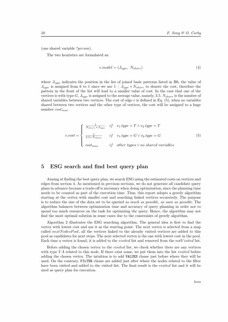
The two heuristics are formulated as:

e.model = (Jtype, Nshare) (4)

where Jtype indicates the position in the list of joined basic patterns listed in H6, the value ofJtype is assigned from 6 to 1 since we use 1 / Jtype ∗ Nshare to denote the cost, therefore thepattern in the front of the list will lead to a smaller value of cost. In the case that one of thevertices is with type G, Jtype is assigned to the average value, namely, 3.5. Nshare is the number ofshared variables between two vertices. The cost of edge e is defined in Eq. (5), when no variablesshared between two vertices and the other type of vertices, the cost will be assigned to a hugenumber costmax.

e.cost =

1

Nshare ∗ Jtypeif v1.type = T ∧ v2.type = T

1

3.5 ∗Nshareif v1.type = G ∨ v2.type = G

costmax if other types ∨ no shared variables

(5)

5 ESG search and find best query plan

Aiming at finding the best query plan, we search ESG using the estimated costs on vertices andedges from section 4. As mentioned in previous sections, we do not generate all candidate queryplans in advance because a trade-off is necessary when doing optimization, since the planning timeneeds to be counted as part of the execution time. Thus, this report adopts a greedy algorithmstarting at the vertex with smaller cost and searching linked vertices recursively. The purposeis to reduce the size of the data set to be queried as much as possible, as soon as possible. Thealgorithm balances between optimization time and accuracy of query planning in order not tospend too much resources on the task for optimizing the query. Hence, the algorithm may notfind the most optimal solution in some cases due to the constraints of greedy algorithm.

Algorithm 2 illustrates the ESG searching algorithm. The general idea is first to find thevertex with lowest cost and use it as the starting point. The next vertex is selected from a mapcalled nextNodesPool, all the vertices linked to the already visited vertices are added to thispool as candidates for next steps. The next selected vertex is the one with lowest cost in the pool.Each time a vertex is found, it is added to the visited list and removed from the notV isited list.

Before adding the chosen vertex to the visited list, we check whether there are any verticeswith type V A related to this node. If there exist some, we put them into the list visited beforeadding the chosen vertex. The intuition is to add VALUES clause just before where they will beused. On the contrary, FILTER clause are added just after where the nodes related to the filterhave been visited and added to the visited list. The final result is the visited list and it will beused as query plan for execution.

Inria

Heuristics-based SPARQL Query Planning 11

Data: ESG = (V,E), V = {v}, E = {e}Data: v = {exp, type,model, cost}, e = {v1, v2, type,model, cost}

1 Initialize empty list visited, notV isited ; vertex first;2 Put all the nodes with type T and G to list notV isited;3 while notVisited is not empty do4 Initialize new Map (vertex, cost) nextNodesPool;5 Find the vertex first with lowest cost from list notV isited;6 Route(first, nextNodesPool);7 end

8 Function Route(previous, nextNodesPool)9 if previous = null then

10 return ;11 end12 Vertex next;13 while (next = FindNext(nextNodesPool)) != null do14 Route(next, nextNodesPool);15 end

16 Function FindNext(nextNodesPool)17 if nextNodesPool is empty then18 return null;19 else20 Find the vertex with the lowest cost from nextNodesPool and assign it to

next ; Queue(next, nextNodesPool);21 return next ;22 end

23 Function Queue(vertex, nextNodesPool)24 For all vertices that have not been visited with type V A linked to vertex, add

them to list visited;25 visited.add(vertex);26 notV isited.remove(vertex);27 For all vertices with type F whose linked vertices all have been visited, add

them to list visited;28 // fill the next nodes pool29 Get the linked edges lEdges of vertex;30 for edge e in lEdges do31 Get the other vertex v2 of e;32 costNew = e.cost ∗ v2.cost;33 if v2 is not visited then34 nextNodesPool.put(v2, costNew);35 end

36 endAlgorithm 2: ESG searching for finding best plan

RR n° 8655

12 F. Song & O. Corby

6 Evaluation

The query planning method described in this report is implemented in Java within CoreseSemantic Web Factory 6. Section 6.1 describes the data set and test cases used. In Section 6.2,we present the results obtained and, based on the results, the discussions and analysis are made.

6.1 Data set and test cases

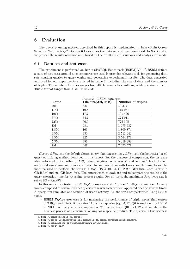
The experiment is performed on Berlin SPARQL Benchmark (BSBM) V3.1 7, BSBM definesa suite of test cases around an e-commerce use case. It provides relevant tools for generating datasets, sending queries to query engine and generating experimental results. The data generatedand used for our experiments are listed in Table 2, including the size of data and the numberof triples. The number of triples ranges from 40 thousands to 7 millions, while the size of file inTurtle format ranges from 4 MB to 647 MB.

Table 2 – BSBM data setsName File size(.ttl, MB) Number of triples40k 3.8 40 377115k 10.8 115 987191k 17.7 191 496374k 34.7 374 911725k 66.6 725 3051M 98.4 1 075 6371.8M 166 1 809 8742.5M 230 2 511 9423.5M 325 3 564 7735.3M 486 5 319 3887M 647 7 073 571

Corese QPv0 uses the default Corese query planning settings. QPv1 uses the heuristics-basedquery optimizing method described in this report. For the purpose of comparison, the tests arealso performed on two other SPARQL query engines: Jena Fuseki 8 and Sesame 9, both of themare tested using in-memory mode in order to compare them with Corese on the same basis.Themachine used to perform the tests is a Mac, OS X 10.9.4, CUP 2.6 GHz Intel Core i5 with 8GB RAM and 500 GB hard disk. The criteria used to evaluate and to compare the results is thequery execution time for returning correct results. For all tests, the maximum Java heap size isset to 8G (-Xmx8G).

In this report, we tested BSBM Explore use case and Business Intelligence use case. A querymix is composed of several distinct queries in which each of them appeared once or several times.A query mix simulates one scenario of user’s activity. All the tests are performed using BSBMtools.

– BSBM Explore uses case is for measuring the performance of triple stores that exposeSPARQL endpoints, it contains 11 distinct queries (Q01-Q12, Q6 is excluded by BSBMin V3.1). A query mix is composed of 25 queries from Q01 to Q12 and simulates thebusiness process of a consumer looking for a specific product. The queries in this use case

6. http://wimmics.inria.fr/corese

7. http://wifo5-03.informatik.uni-mannheim.de/bizer/berlinsparqlbenchmark/

8. http://jena.apache.org/documentation/serving_data/

9. http://rdf4j.org/

Inria

Heuristics-based SPARQL Query Planning 13

are relatively simple (rather flat, do not contain nested query) and take little time, so thisuse case is used for evaluating the described QP approach by comparing to the originalsystem QPv0. The purpose is to see the effects of the proposed approach since except forthe QP approach, the other aspects are identical, such as the data storage and indexingmechanism, query processing, etc.

– BSBM Business Intelligence use case simulates different stakeholders asking analytic ques-tions against the data set. The query mix consists of 8 distinct queries (Qb1 - Qb8), eachquery mix contains 15 queries. The queries in this use case are relatively complex andtake longer time. This use case is used for comparing Corese with the other systems: Jenaand Sesame to see the performance difference.

6.2 Results and discussion

The QP strategy of QPv1 in Corese is that first we try to apply the QPv1, but if it is notapplicable, then we will turn to QPv0. Thus for a SPARQL query containing multiple ESGs, twoQP strategies might be applied. For the Explore use case, we focus on analyzing the queries thathave been rewritten by QPv1 to see whether the proposed method is useful. For the BusinessIntelligence use case, we emphasize on comparing Corese system (taking as a whole) with theother systems.

6.2.1 BSBM Explore use case

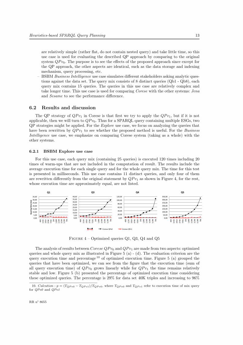
For this use case, each query mix (containing 25 queries) is executed 120 times including 20times of warm-ups that are not included in the computation of result. The results include theaverage execution time for each single query and for the whole query mix. The time for this testis presented in milliseconds. This use case contains 11 distinct queries, and only four of themare rewritten differently from the original statement by QPv1 as shown in Figure 4, for the rest,whose execution time are approximately equal, are not listed.

0,00#

5,00#

10,00#

15,00#

20,00#

25,00#

30,00#

35,00#

40K#

115K#

191K#

374K#

725K#

1M#

1,8M#

2,5M#

3,5M#

5,3M#

7M#

Quering()me((ms)(

Q1(

0,00#

5,00#

10,00#

15,00#

20,00#

25,00#

30,00#

35,00#

40,00#

40K#

115K#

191K#

374K#

725K#

1M#

1,8M#

2,5M#

3,5M#

5,3M#

7M#

Q3(

0,00#

20,00#

40,00#

60,00#

80,00#

100,00#

120,00#

40K#

115K#

191K#

374K#

725K#

1M#

1,8M#

2,5M#

3,5M#

5,3M#

7M#

Q4(

0,00#

50,00#

100,00#

150,00#

200,00#

250,00#

300,00#

350,00#

40K#

115K#

191K#

374K#

725K#

1M#

1,8M#

2,5M#

3,5M#

5,3M#

7M#

Q5(

Corese#QPv0# Corese#QPv1#

Figure 4 – Optimized queries Q1, Q3, Q4 and Q5

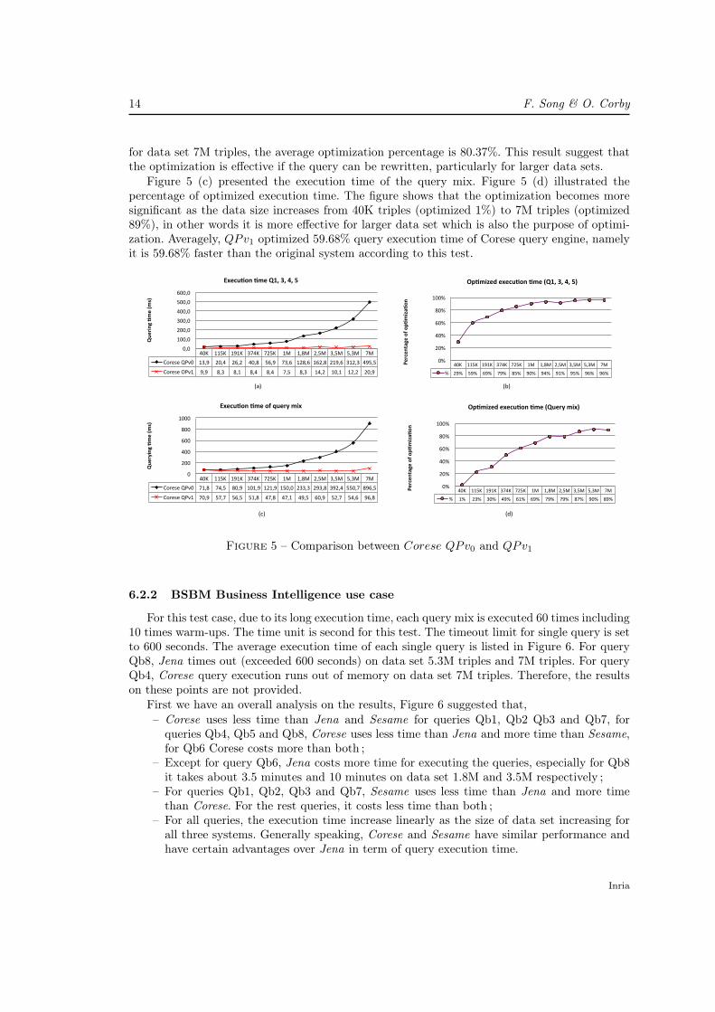
The analysis of results between Corese QPv0 and QPv1 are made from two aspects: optimizedqueries and whole query mix as illustrated in Figure 5 (a) - (d). The evaluation criterion are thequery execution time and percentage 10 of optimized execution time. Figure 5 (a) grouped thequeries that have been optimized, we can see from the figure that the execution time (sum ofall query execution time) of QPv0 grows linearly while for QPv1 the time remains relativelystable and low. Figure 5 (b) presented the percentage of optimized execution time consideringthese optimized queries. The percentage is 29% for data set 40K triples and increasing to 96%

10. Calcution : p = (TQPv0 − TQPv1)/TQPv0, where TQPv0 and TQPv1 refer to execution time of mix query

for QPv0 and QPv1

RR n° 8655

14 F. Song & O. Corby

for data set 7M triples, the average optimization percentage is 80.37%. This result suggest thatthe optimization is effective if the query can be rewritten, particularly for larger data sets.

Figure 5 (c) presented the execution time of the query mix. Figure 5 (d) illustrated thepercentage of optimized execution time. The figure shows that the optimization becomes moresignificant as the data size increases from 40K triples (optimized 1%) to 7M triples (optimized89%), in other words it is more effective for larger data set which is also the purpose of optimi-zation. Averagely, QPv1 optimized 59.68% query execution time of Corese query engine, namelyit is 59.68% faster than the original system according to this test.

40K$ 115K$ 191K$ 374K$ 725K$ 1M$ 1,8M$ 2,5M$ 3,5M$ 5,3M$ 7M$

Corese$QPv0$ 71,8$ 74,5$ 80,9$ 101,9$ 121,9$ 150,0$ 233,3$ 293,8$ 392,4$ 550,7$ 896,5$

Corese$QPv1$ 70,9$ 57,7$ 56,5$ 51,8$ 47,8$ 47,1$ 49,5$ 60,9$ 52,7$ 54,6$ 96,8$

0$

200$

400$

600$

800$

1000$

Querying)*me)(ms))

Execu*on)*me)of)query)mix)

40K$ 115K$ 191K$ 374K$ 725K$ 1M$ 1,8M$ 2,5M$ 3,5M$ 5,3M$ 7M$

Corese$QPv0$ 13,9$ 20,4$ 26,2$ 40,8$ 56,9$ 73,6$ 128,6$ 162,8$ 219,6$ 312,3$ 495,5$

Corese$OPv1$ 9,9$ 8,3$ 8,1$ 8,4$ 8,4$ 7,5$ 8,3$ 14,2$ 10,1$ 12,2$ 20,9$

0,0$

100,0$

200,0$

300,0$

400,0$

500,0$

600,0$

Quering)*me)(ms))

Execu*on)*me)Q1,)3,)4,)5)

40K$ 115K$ 191K$ 374K$ 725K$ 1M$ 1,8M$ 2,5M$ 3,5M$ 5,3M$ 7M$

%$ 1%$ 23%$ 30%$ 49%$ 61%$ 69%$ 79%$ 79%$ 87%$ 90%$ 89%$

0%$

20%$

40%$

60%$

80%$

100%$

Percentage)of)op*miza*on)

Op*mized)execu*on)*me)(Query)mix))

(a)$$$$$$$$$$$$$$$$$$$$$$$$$$$$$$$$$$$$$$$$$$$$$$$$$$$$$$$$$$$$$$$$$$$$$$$$$$$$$$$$$$$$$$$$$$$$$$$$$$$$$$$$$$$$$$$$$$$$$$$$$$$$$$$$$$$$$$$$$$$$$$$$$$$$$$$$$$$$$$$$$$$$$$(b)$$$$$$$$$$$$$$$$$$$$$$$$$$$$$$$$$$$$$$$$$$$$$$$$$$$$$$$$$$$$$$$$$$$$$$$$$$$$$$$

(c)$$$$$$$$$$$$$$$$$$$$$$$$$$$$$$$$$$$$$$$$$$$$$$$$$$$$$$$$$$$$$$$$$$$$$$$$$$$$$$$$$$$$$$$$$$$$$$$$$$$$$$$$$$$$$$$$$$$$$$$$$$$$$$$$$$$$$$$$$$$$$$$$$$$$$$$$$$$$$$$$$$$$$(d)$$$$$$$$$$$$$$$$$$$$$$$$$$$$$$$$$$$$$$$$$$$$$$$$$$$$$$$$$$$$$$$$$$$$$$$

40K$ 115K$ 191K$ 374K$ 725K$ 1M$ 1,8M$ 2,5M$ 3,5M$ 5,3M$ 7M$

%$ 29%$ 59%$ 69%$ 79%$ 85%$ 90%$ 94%$ 91%$ 95%$ 96%$ 96%$

0%$

20%$

40%$

60%$

80%$

100%$

Percentage)of)op*miza*on)

Op*mized)execu*on)*me)(Q1,)3,)4,)5))

Figure 5 – Comparison between Corese QPv0 and QPv1

6.2.2 BSBM Business Intelligence use case

For this test case, due to its long execution time, each query mix is executed 60 times including10 times warm-ups. The time unit is second for this test. The timeout limit for single query is setto 600 seconds. The average execution time of each single query is listed in Figure 6. For queryQb8, Jena times out (exceeded 600 seconds) on data set 5.3M triples and 7M triples. For queryQb4, Corese query execution runs out of memory on data set 7M triples. Therefore, the resultson these points are not provided.

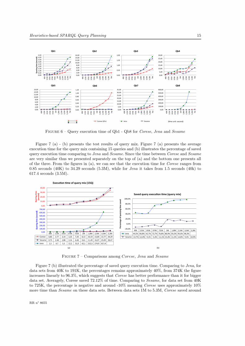
First we have an overall analysis on the results, Figure 6 suggested that,– Corese uses less time than Jena and Sesame for queries Qb1, Qb2 Qb3 and Qb7, for

queries Qb4, Qb5 and Qb8, Corese uses less time than Jena and more time than Sesame,for Qb6 Corese costs more than both ;

– Except for query Qb6, Jena costs more time for executing the queries, especially for Qb8it takes about 3.5 minutes and 10 minutes on data set 1.8M and 3.5M respectively ;

– For queries Qb1, Qb2, Qb3 and Qb7, Sesame uses less time than Jena and more timethan Corese. For the rest queries, it costs less time than both ;

– For all queries, the execution time increase linearly as the size of data set increasing forall three systems. Generally speaking, Corese and Sesame have similar performance andhave certain advantages over Jena in term of query execution time.

Inria

Heuristics-based SPARQL Query Planning 15

0,00#

0,50#

1,00#

1,50#

2,00#

2,50#

3,00#

3,50#

4,00#

4,50#

40K#

115K#

191K#

374K#

725K#

1M#

1,8M#

2,5M#

3,5M#

5,3M#

7M#

Quering()me((second)(

Qb1(

0,00#

2,00#

4,00#

6,00#

8,00#

10,00#

12,00#

14,00#

16,00#

40K#

115K#

191K#

374K#

725K#

1M#

1,8M#

2,5M#

3,5M#

5,3M#

7M#

Qb2(

0,00#

0,50#

1,00#

1,50#

2,00#

40K#

115K#

191K#

374K#

725K#

1M#

1,8M#

2,5M#

3,5M#

5,3M#

7M#

Qb3(

0,00#

5,00#

10,00#

15,00#

20,00#

25,00#

30,00#

40K#

115K#

191K#

374K#

725K#

1M#

1,8M#

2,5M#

3,5M#

5,3M#

7M#

Qb4(

0,00#

2,00#

4,00#

6,00#

8,00#

10,00#

12,00#

14,00#

16,00#

40K#

115K#

191K#

374K#

725K#

1M#

1,8M#

2,5M#

3,5M#

5,3M#

7M#

Qb5(

0,00#

0,20#

0,40#

0,60#

0,80#

1,00#

1,20#

40K#

115K#

191K#

374K#

725K#

1M#

1,8M#

2,5M#

3,5M#

5,3M#

7M#

Qb6(

0,00#

5,00#

10,00#

15,00#

20,00#

25,00#

30,00#

35,00#

40K#

115K#

191K#

374K#

725K#

1M#

1,8M#

2,5M#

3,5M#

5,3M#

7M#

Qb7(

0,00#

100,00#

200,00#

300,00#

400,00#

500,00#

600,00#

40K#

115K#

191K#

374K#

725K#

1M#

1,8M#

2,5M#

3,5M#

5,3M#

7M#

Qb8(

Corese#QPv1# Jena# Sesame# (=me#unit:#second)#

Figure 6 – Query execution time of Qb1 - Qb8 for Corese, Jena and Sesame

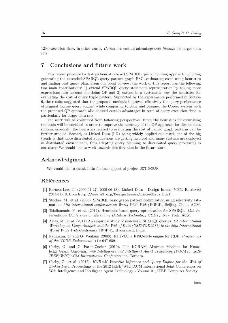
Figure 7 (a) - (b) presents the test results of query mix. Figure 7 (a) presents the averageexecution time for the query mix containing 15 queries and (b) illustrates the percentage of savedquery execution time comparing to Jena and Sesame. Since the time between Corese and Sesameare very similar thus we presented separately on the top of (a) and the bottom one presents allof the three. From the figures in (a), we can see that the execution time for Corese ranges from0.85 seconds (40K) to 34.29 seconds (5.3M), while for Jena it takes from 1.5 seconds (40k) to617.4 seconds (3.5M).

40K$ 115K$ 191K$ 374K$ 725K$ 1M$ 1,8M$ 2,5M$ 3,5M$ 5,3M$

Corese$ 0,85$ 2,77$ 3,14$ 3,33$ 7,20$ 8,13$ 10,19$ 13,69$ 22,77$ 34,29$

Sesame$ 0,75$ 2,48$ 2,88$ 3,16$ 6,48$ 9,61$ 11,49$ 16,07$ 25,09$ 38,47$

Jena$ 1,5$ 4,7$ 5,5$ 12,2$ 31,0$ 62,1$ 152,5$ 274,9$ 617,4$

0,00$

100,00$

200,00$

300,00$

400,00$

500,00$

600,00$

700,00$

Quering()me((second)(

Execu)on()me(of(query(mix((15Q)(

40K$ 115K$ 191K$ 374K$ 725K$ 1M$ 1,8M$ 2,5M$ 3,5M$ 5,3M$

Jena$ 44,5%$ 40,8%$ 42,7%$ 72,7%$ 76,8%$ 86,9%$ 93,3%$ 95,0%$ 96,3%$

Sesame$ :13,7%$ :12,0%$ :9,1%$ :5,4%$ :11,1%$ 15,4%$ 11,3%$ 14,8%$ 9,3%$ 10,9%$

:20,0%$

0,0%$

20,0%$

40,0%$

60,0%$

80,0%$

100,0%$

Percentage(of(querying()me(saved(

Saved(query(execu)on()me((query(mix)(

(a)$$$$$$$$$$$$$$$$$$$$$$$$$$$$$$$$$$$$$$$$$$$$$$$$$$$$$$$$$$$$$$$$$$$$$$$$$$$$$$$$$$$$$$$$$$$$$$$$$$$$$$$$$$$$$$$$$$$$$$$$$$$$$$$$$$$$$$$$$$$$$$$$$$$$$$$$$$$$$$$$$$$$$$$$$$$(b)$$$$$$$$$$$$$$$$$$$$$$$$$$$$$$$$$$$$$$$$$$$$$$$$$$$$$$$$$$$$$$$$$$$$$$$$$$$$$$$

0,00$

10,00$

20,00$

30,00$

40,00$

Quering()me(

(second)(

Figure 7 – Comparisons among Corese, Jena and Sesame

Figure 7 (b) illustrated the percentage of saved query execution time. Comparing to Jena, fordata sets from 40K to 191K, the percentages remains approximately 40%, from 374K the figureincreases linearly to 96.3%, which suggests that Corese has better performance than it for biggerdata set. Averagely, Corese saved 72.12% of time. Comparing to Sesame, for data set from 40Kto 725K, the percentage is negative and around -10% meaning Corese uses approximately 10%more time than Sesame on these data sets. Between data sets 1M to 5.3M, Corese saved around

RR n° 8655

16 F. Song & O. Corby

12% execution time. In other words, Corese has certain advantage over Sesame for larger datasets.

7 Conclusions and future work

This report presented a 3-steps heuristic-based SPARQL query planning approach includinggenerating the extended SPARQL query pattern graph ESG, estimating costs using heuristicsand finding best query plan. From our point of view, the work of this report has the followingtwo main contributions: 1) extend SPARQL query statement representation by taking moreexpressions into account for doing QP and 2) extend in a systematic way the heuristics forevaluating the cost of query triple pattern. Supported by the experiments performed in Section6, the results suggested that the proposed methods improved effectively the query performanceof original Corese query engine, while comparing to Jena and Sesame, the Corese system withthe proposed QP approach also showed certain advantages in term of query execution time inparticularly for larger data sets.

The work will be continued from following perspectives. First, the heuristics for estimatingthe costs will be enriched in order to improve the accuracy of the QP approach for diverse datasources, especially the heuristics related to evaluating the cost of named graph patterns can befurther studied. Second, as Linked Data (LD) being widely applied and used, one of the bigtrends is that more distributed applications are getting involved and many systems are deployedin distributed environment, thus adapting query planning to distributed query processing isnecessary. We would like to work towards this direction in the future work.

Acknowledgment

We would like to thank Inria for the support of project ADT KGRAM.

Références

[1] Berners-Lee, T. (2006-07-27, 2009-06-18). Linked Data - Design Issues. W3C. Retrieved2014-11-18, from http://www.w3.org/DesignIssues/LinkedData.html.

[2] Stocker, M., et al. (2008). SPARQL basic graph pattern optimization using selectivity esti-mation. 17th international conference on World Wide Web (WWW), Beijing, China, ACM.

[3] Tsialiamanis, P., et al. (2012). Heuristics-based query optimisation for SPARQL. 15th In-ternational Conference on Extending Database Technology (ICDT), New York, ACM.

[4] Arias, M., et al. (2011).An empirical study of real-world SPARQL queries. 1st InternationalWorkshop on Usage Analysis and the Web of Data (USEWOD2011) in the 20th InternationalWorld Wide Web Conference (WWW), Hyderabad, India.

[5] Neumann, T. and G. Weikum (2008). RDF-3X: a RISC-style engine for RDF. Proceedingsof the VLDB Endowment 1(1): 647-659.

[6] Corby, O. and C. Faron-Zucker (2010). The KGRAM Abstract Machine for Know-ledge Graph Querying. Web Intelligence and Intelligent Agent Technology (WI-IAT), 2010IEEE/WIC/ACM International Conference on, Toronto.

[7] Corby, O., et al. (2012). KGRAM Versatile Inference and Query Engine for the Web ofLinked Data. Proceedings of the 2012 IEEE/WIC/ACM International Joint Conferences onWeb Intelligence and Intelligent Agent Technology - Volume 01, IEEE Computer Society.

Inria

Heuristics-based SPARQL Query Planning 17

[8] Chaudhuri, S. (1998). An overview of query optimization in relational systems. the 17thACM SIGACT-SIGMOD-SIGART symposium on Principles of database systems, Seattle,Washington, USA, ACM.

[9] Liu, C., et al. (2010). Towards efficient SPARQL query processing on RDF data. TsinghuaScience & Technology 15(6): 613-622.

[10] Huang, H. and C. Liu (2010). Selectivity estimation for SPARQL graph pattern. 19th in-ternational conference on World Wide Web (WWW2010), Raleigh, North Carolina, USA,ACM.

[11] Poosala, V., et al. (1996). Improved histograms for selectivity estimation of range predicates.ACM SIGMOD Record 25(2): 294-305.

[12] Harary, F. (1994). Graph Theory, Perseus Books.

RR n° 8655

RESEARCH CENTRE

SOPHIA ANTIPOLIS – MÉDITERRANÉE

2004 route des Lucioles - BP 93

06902 Sophia Antipolis Cedex

Publisher

Inria

Domaine de Voluceau - Rocquencourt

BP 105 - 78153 Le Chesnay Cedex

inria.fr

ISSN 0249-6399