hfodudwlyh 0rghov iru 6hoi &doleudwlqj...

Abstract

The use of industrial robots in manufacturing often requires good calibration ap-proaches and tools to obtain and maintain the desirable accuracy of the robot, forthe robot to be able to execute a task in a satisfactory manner. For high-accuracymethods of calibration, it is necessary to first identify the robot’s stiffness param-eters. This thesis will focus on a method that is based on a clamping procedure.In this procedure, the robot’s end effector is clamped to a fixed object and load isapplied by the motors of the joints while measurements of torque and position ofthe motors are performed by the robot’s own sensors. These measurements are thenused to identify the stiffness parameters of the robot. The purpose of this thesis isto develop a model library written in the modeling language Modelica to be usedfor robot simulations, and especially to simulate these clamping experiments. Inthe modeling, focus will lie on dynamical behaviour like compliance, backlash, andfriction and how these effect the results of the clamping experiments.

The modularity aspect has been a central part in the progress and the modellibrary developed is component based, i.e., the parts can be connected in variousways to model different types of robots. For model validation, many simulationshave been performed with different dynamic model parameters to evaluate the re-sults and how they compare to the expected dynamic behaviour. Also, experimentaldata from experiments with ABB’s robot IRB140 have been used to judge how wellthe models can reproduce results from real experiments.

The simulation results indicate that the models capture much of the dynamicalbehaviour in a satisfying way. The effects of joint compliance, friction, backlash,compliance in the clamping device, and variations in the clamping configurationare all of importance for the results of the clamping simulations. When comparingto data provided from clamping experiments of the IRB140 robot, the results ofthe simulations show that the models are able to reproduce much of the robot’sbehaviour observed in the experiments.

Keywords: Robotics, Robot Modeling, Robot Calibration, Self-Calibrating Robots,Clamping, Declarative Modeling, Modelica.

3

Acknowledgments

This thesis was written during the fall of 2016 at the Department of AutomaticControl at Lund University, in cooperation with Cognibotics AB, Lund.

We are very grateful to our supervisor Björn Olofsson for his exceptional sup-port during the work with this thesis. Our assisting supervisors at Cognibotics AB,Andreas Stolt and Olof Sörnmo, are acknowledged for their valuable suggestionsand inputs. Also, we would like to thank Klas Nilsson and Cognibotics AB for giv-ing us the opportunity to write this thesis.

We would like to thank our wonderful friends and families for their great sup-port throughout our studies at Lund University. A special thanks to Rebecca Tencic,William Lindeberg, Gustav Ek, Jonas Eliasson, Niklas Hansson, Emma Sjöborg,and Filip Thor for their invaluable friendship and for motivating us to alwaysperform at our best. Niklas and Filip have also been great lunch partners at theuniversity and have inspired us during the work with this thesis.

Lund, February 2017Johannes Olsson and Pontus Sikström

5

Contents

1. Introduction 91.1 Background . . . . . . . . . . . . . . . . . . . . . . . . . . . . 91.2 Problem Formulation . . . . . . . . . . . . . . . . . . . . . . . 91.3 Subject Foundation . . . . . . . . . . . . . . . . . . . . . . . . 101.4 Delimitations . . . . . . . . . . . . . . . . . . . . . . . . . . . . 10

2. Theory 122.1 Manipulator Basics . . . . . . . . . . . . . . . . . . . . . . . . 122.2 Wrists . . . . . . . . . . . . . . . . . . . . . . . . . . . . . . . 132.3 Clamping Experiments . . . . . . . . . . . . . . . . . . . . . . 152.4 Newton-Euler Formulation . . . . . . . . . . . . . . . . . . . . 162.5 Elasticity Models . . . . . . . . . . . . . . . . . . . . . . . . . 182.6 Friction . . . . . . . . . . . . . . . . . . . . . . . . . . . . . . . 182.7 Backlash . . . . . . . . . . . . . . . . . . . . . . . . . . . . . . 192.8 Controller . . . . . . . . . . . . . . . . . . . . . . . . . . . . . 202.9 Modelica Language . . . . . . . . . . . . . . . . . . . . . . . . 21

3. Modelling 243.1 Overview . . . . . . . . . . . . . . . . . . . . . . . . . . . . . . 253.2 Frame (connector) . . . . . . . . . . . . . . . . . . . . . . . . . 263.3 Inertial Frame . . . . . . . . . . . . . . . . . . . . . . . . . . . 273.4 Flange (connector) . . . . . . . . . . . . . . . . . . . . . . . . . 273.5 Link . . . . . . . . . . . . . . . . . . . . . . . . . . . . . . . . 273.6 Joint . . . . . . . . . . . . . . . . . . . . . . . . . . . . . . . . 273.7 Revolute Joint . . . . . . . . . . . . . . . . . . . . . . . . . . . 283.8 Revolute Axis . . . . . . . . . . . . . . . . . . . . . . . . . . . 293.9 Clamping Device . . . . . . . . . . . . . . . . . . . . . . . . . 323.10 Controller . . . . . . . . . . . . . . . . . . . . . . . . . . . . . 323.11 Path Planning . . . . . . . . . . . . . . . . . . . . . . . . . . . 333.12 Wrist . . . . . . . . . . . . . . . . . . . . . . . . . . . . . . . . 35

4. Results 364.1 Dymola and JModelica.org . . . . . . . . . . . . . . . . . . . . 36

7

Contents

4.2 ABB IRB140 Experiments . . . . . . . . . . . . . . . . . . . . 374.3 Simulation Setup . . . . . . . . . . . . . . . . . . . . . . . . . . 394.4 Joint Compliance . . . . . . . . . . . . . . . . . . . . . . . . . 434.5 Friction . . . . . . . . . . . . . . . . . . . . . . . . . . . . . . . 454.6 Backlash . . . . . . . . . . . . . . . . . . . . . . . . . . . . . . 484.7 Orthogonal Compliance . . . . . . . . . . . . . . . . . . . . . . 504.8 Compliance in the Clamped End . . . . . . . . . . . . . . . . . 524.9 Clamping Configuration . . . . . . . . . . . . . . . . . . . . . . 534.10 Simulated Results Compared to Experimental Data . . . . . . . 55

5. Discussion and Conclusions 585.1 Simulation Results . . . . . . . . . . . . . . . . . . . . . . . . . 585.2 Friction . . . . . . . . . . . . . . . . . . . . . . . . . . . . . . . 595.3 Link Elasticity . . . . . . . . . . . . . . . . . . . . . . . . . . . 595.4 Joint Types . . . . . . . . . . . . . . . . . . . . . . . . . . . . . 605.5 Future Work . . . . . . . . . . . . . . . . . . . . . . . . . . . . 605.6 Conclusions . . . . . . . . . . . . . . . . . . . . . . . . . . . . 60

Bibliography 62A. Modelica Models 64

A.1 Frame . . . . . . . . . . . . . . . . . . . . . . . . . . . . . . . 64A.2 InertialFrame . . . . . . . . . . . . . . . . . . . . . . . . . . . . 64A.3 Flange . . . . . . . . . . . . . . . . . . . . . . . . . . . . . . . 65A.4 Link . . . . . . . . . . . . . . . . . . . . . . . . . . . . . . . . 65A.5 Joint . . . . . . . . . . . . . . . . . . . . . . . . . . . . . . . . 66A.6 RevoluteJoint . . . . . . . . . . . . . . . . . . . . . . . . . . . 67A.7 RevoluteAxis . . . . . . . . . . . . . . . . . . . . . . . . . . . 69A.8 Motor . . . . . . . . . . . . . . . . . . . . . . . . . . . . . . . 70A.9 Gear . . . . . . . . . . . . . . . . . . . . . . . . . . . . . . . . 70A.10 ControlBus . . . . . . . . . . . . . . . . . . . . . . . . . . . . . 71A.11 ClampingPoint . . . . . . . . . . . . . . . . . . . . . . . . . . . 71A.12 Controller . . . . . . . . . . . . . . . . . . . . . . . . . . . . . 72A.13 Wrist . . . . . . . . . . . . . . . . . . . . . . . . . . . . . . . . 73A.14 ClampingPathPlanning . . . . . . . . . . . . . . . . . . . . . . 74A.15 getOrthVectors . . . . . . . . . . . . . . . . . . . . . . . . . . . 75

8

1Introduction

This chapter introduces the background and describes the purpose of this thesis. Thedelimitations of the work will also be set.

1.1 Background

The demand for industrial robots has increased drastically the past decade. Between2010 and 2015, the average robot sales increase per year was at 16% worldwide andthis increase is predicted to continue the coming years [World Robotics 2016]. Withhigher sales and more application scopes added for each year, the demand for highaccuracy also increases. One advantage of high-accuracy robots is that they can beprogrammed to reach certain positions in a reference coordinate system with goodaccuracy without being manually taught the positions. This reduces the need forhuman assistance when training a robot to perform a task.

Reliable calibration methods and tools are important to achieve and maintainhigh precision and accuracy. There are many different such calibration methodsand this thesis focuses on a method that is based on experiments performed whilethe robots end-effector is clamped to a fixed object. By giving angle references tothe regulator of the joints, while the end effector is clamped to a fixed point inspace, it is possible to identify compliance in the joints that are trying to move.The measurements can be done with the robot’s sensors alone, without any need forexternal equipment, this is what makes the robot self-calibrating. This is a majoradvantage of this type of calibration method compared to many other calibrationmethods which often need expensive external equipment, like advanced cameras tomeasure the positions and orientations of different parts of the robot.

1.2 Problem Formulation

To be able to make relevant simulations regarding the precision and accuracy ofrobots, good models are required. It is desirable to be able to experiment with iden-tification algorithms on models, instead of on actual manipulators, to estimate elas-

9

Chapter 1. Introduction

ticity parameters and other relevant dynamics. A suitable model library can also beused to find models where simulation results correspond to experimental data. Itis both cheaper and more convenient to use computer simulations as an alternativeto experiments on actual manipulators. Additionally, robot models can be used topredict the movement of a robot that in a certain task is experiencing external forcesand torques. This prediction can be important when working with computer toolssuch as CAM (Computer-Aided Manufacturing).

The overall purpose of this thesis is to develop a Modelica library used for mod-eling and simulating manipulators. The models should be able to simulate clampingexperiments of the robots, with results close to the results of experiments with ac-tual robots. Another important aspect is the modularity, i.e., the manipulator modelsshould be component based and it should be easy to modify the structure and com-ponent parameters to simulate different types of robots. Good models can be a greataid in the work to determine which dynamical effects of the manipulator that giverise to what kind of effects in the experiment data. This could lead to a better un-derstanding of the resulting data from clamping experiments.

1.3 Subject Foundation

The work of this thesis has been carried out in cooperation with the company Cog-nibotics. Cognibotics is a company based in Lund, Sweden that specializes in meth-ods and services for determination of robot properties such as backlash, friction, andnon-linear compliance and improving robot accuracy in applications [Cognibotics,2017]. One of the techniques investigated by the company is based on the methoddescribed in Section 1.1, where the robot’s end-effector is clamped fixed to anotherstiff object. It is of interest to evaluate how dynamic models of the robot, definedin a declarative modeling language, can be of use both in the identification phaseand the subsequent calibration and pose compensation phases. This question is thefoundation of this thesis. A description of the methods used for determination ofrobot properties can be found in [Nilsson, 2012].

The importance of different dynamical phenomena in robot models has beenresearched at Linköping University in the Master Thesis [Niglis and Öberg, 2015]with many topics associated to the work in this thesis. The thesis from LinköpingUniversity discusses friction and elasticity in greater depth while the work of thisthesis is more focused around the implementation of the models. Also, a differentmodel language, Simulink [Simulink], is used in the Linköping thesis.

1.4 Delimitations

Robot modeling is a very complex subject and the work with a model library as theone developed in this thesis needs to be delimited in some aspects for the task to beaccomplished within the time frame of the thesis.

10

1.4 Delimitations

The models will only support one kind of joints, the revolute joint. This is themost common joint type for industrial robots [Ross et al., 2011, Ch. 2]. Other typesof joints that are common in robots are prismatic, spherical, and helical joints, butmodeling of these is not covered in this thesis.

The kinematics and dynamics of parallel manipulators will not be covered either.This means that the model library only supports modeling of serial manipulators(robots with links connected in series).

Compliance is a dynamic behaviour of great importance when modelling robots.The compliance is typically caused by the components of the joints—the gearbox,for example—and by link elasticity. In this thesis, only joint compliance will beconsidered. Both compliance in the rotational direction of the revolute joint and indirections orthogonal to this are included. The links will be considered as stiff andthus, link elasticity will not be modeled.

The modelling language Modelica is used for all the modeling in this thesis.Other simulation tools, like Simulink [Simulink], could have been tried as well butModelica was judged to be the preferred one. Modelica supports DAE-based (dif-ferential algebraic equation) modelling which means that both ODEs (ordinay dif-ferential equation) and algebraic states can be used. This is an advantage compareto simulation tools that only support ODEs, since it often demands more of the userwhen not being able to use algebraic states in the model equation set-up.

and a description of some of the advantages of Modelica can be found in Section2.9.

11

2Theory

This chapter provides basic information about robot manipulators in general andabout the clamping experiments that this thesis will revolve around. Some theoryabout the dynamics that are used in the models will also be explained. Furthermore,an introduction to the modelling language Modelica, that is used to implement themodels, is presented.

2.1 Manipulator Basics

The type of robots the models in this thesis describe are often referred to as ma-nipulators and are built up by links and joints. There are many different types ofjoints, but in this thesis only revolute joints are concerned. A revolute joint is aone-degree-of-freedom kinematic pair which provides rotation around a single axis[Spong et al., 2005, p. 3-4], as illustrated in Figure 2.1.

Figure 2.1 2D representation of a revolute joint, where the arrow illustrates therotation.

Links refer to the body parts between the joints (or, if the first or the last link,between a joint and a fixed/free end).

To be able to express the position and orientation of different parts of the robot,a set of coordinate frames is needed. Every coordinate frame is fixed to a certainpart of the robot and if that part rotates or moves, the coordinate frame does so as

12

2.2 Wrists

well (and other frames connected to that frame). The inertial frame is the referencecoordinate frame which can be seen as fixed to the ground. This frame never movesor rotates.

A sketch of a simple manipulator with three joints and three links can be seenin Figure 2.2. The frame x0y0z0 is fixed, both in position and rotation, and canbe seen as the end of the base link which is fixed to the ground. The three jointshave one degree of freedom each and the state variable qi represents the rotationangle (relative to starting position). The variable q1 represents a rotation around they0 axis, while q2 and q3 rotate around z1 and z2, respectively. The three links arerepresented by the length vectors l1, l2, and l3. Each coordinate frame xiyizi is fixedto the end of link i. This means that a rotation of the first joint by an angle q1 leadsto a rotation (relative the frame x0y0z0) of the frames x1y1z1 and x2y2z2, while theframe x3y3z3 is subject to both a rotation and a change of position.

The coordinate system conventionally used for robot manipulators uses the samex-axis but is rotated −π/2 radians around the x-axis. Our unconventional choice ofcoordinate system with the y-axis pointing upwards (see Figure 2.2) is used forthe manipulators throughout this thesis. The reason for this is to simplify compar-isons with models from the Modelica standard library which uses this convention[Modelica language specification, 2014]. A lot of these comparisons were made inthe beginning of the modeling, to validate the basics of the kinematic behavior andforce transmission of the link/joint systems.

2.2 Wrists

The joints that control the orientation of the end-effector, located after the mainjoints of the manipulator, are usually referred to as the wrist of the manipulator. Thejoints in the wrist are most often of the revolute type and if their axes of rotationintersect at a common point in space they are referred to as a spherical wrist. Spher-ical wrists are becoming increasingly more popular [Spong et al., 2005]. While thefirst three joints of the manipulator are responsible for determining the position ofthe end effector, the wrist is what decides the orientation. There is often not enoughroom for all motors in the actual wrist, so they are many times located elsewhere onthe manipulator, often closer to the base of the robot. In these cases, a mechanicaltrain of gears are used to drive the wrist and the motors often result in motion inmore than one of the joints in the wrist. With these configurations, a transmissionmatrix needs to be defined to describe the kinematic coupling of the wrist. This ma-trix is used to specify the relationships between the driving motors and the joints inthe wrist by the relations

qarm = Gqmotor (2.1)

τmotor = GTτarm (2.2)

13

Chapter 2. Theory

Figure 2.2 A sketch of a simple manipulator setup with three joints and three links.

14

2.3 Clamping Experiments

where qarm and qmotor are the three motor positions and three joint positions re-spectively, while τmotor and τarm are the three motor torques and three joint torques,respectively. G is the transmission matrix [Asada, 2005, Ch. 6].

2.3 Clamping Experiments

To accurately calibrate a robot, it is sometimes necessary to first identify the robot’sstiffness parameters, to manage to compensate for geometrical deviations that oc-curs because of gravity or process forces. This can be done in many different waysand most methods use external devices to apply loads to components of the robotand to measure positions. However, the clamping method concerned in this thesisdoes not need any external devices, since the loads are applied by the robot’s ownactuators and all measurements are done by the robot’s own sensors. The stiffnessparameters are estimated with the end-effector clamped to a fixed object.

Figure 2.3 Setup for clamping [Nilsson, 2012]

In the test setup in Figure 2.3, the end-effector 16 will be clamped to the fixedpoint 17. The measurements for identifying the stiffness parameters for one joint

15

Chapter 2. Theory

are then acquired by using the motor of that joint’s axis to apply a load while thestructure is clamped. All movements in the structure are then results of the elasticityof the components and not of joint movement. To get enough data for parameter es-timation, the robot is clamped to a set of different fixed positions and measurementsare done while applying loads to the different joints.

2.4 Newton-Euler Formulation

In the model library developed for this thesis, the Newton-Euler formulation [Sponget al., 2005, p. 215] is used to compute the force and torque affecting the links ofthe manipulator due to linear and angular motions. The Newton-Euler formulationis different from other common methods, like the Lagrangian formulation [Sponget al., 2005, p. 188], in the way that it uses a forward-backward recursion to analyzethe force and the torque. This approach means that it treats one link at a time, toeventually be able to describe the manipulator as a whole, in contrary to the La-grangian formulation where the states of all links are needed simultaneously to per-form the analysis. In the Newton-Euler formulation, the equations are evaluated in anumeric way and the computational complexity in each step remains constant. Thismeans that the computational complexity grows in a linear fashion with the numberN of joints and is computationally advantageous to other methods [Newton-Eulerapproach, 2016]. The Newton-Euler formulation also makes it easier to implementthe models more genericly, since it is not as dependent of the manipulator setup asa whole to compute force and torque because all the computations are performed ineach link separately. But of course, the forces and torques in one link depend on theforces and torques in neighbouring links. Before going into detail on the equations,some notations are introduced. Here frame i is a coordinate frame that is rigidlyattached to link i. Beginning link means the side closest to the base and end of thelink is the side closest to the end-effector of the manipulator. The variables in the

16

2.4 Newton-Euler Formulation

formulation are as follows:

fi = force exerted by link i−1, resolved in frame i.τi = torque exerted by link i−1, resolved in frame i.

f ii+1 = force exerted by link i+1, resolved in frame i.

τii+1 = torque exerted by link i+1, resolved in frame i.mi = mass of link i.

ac,i = acceleration of the center of mass of link i, resolved in frame i.gi = acceleration due to gravity in frame i.

ri,ci = vector from beginning of link i to the center of mass of link i in frame i.

rii+1,ci = vector from end of link i to the center of mass of link i in frame i.

ωi = angular velocity of frame i with respect to the inertial frame resolved inframe i.

αi = angular acceleration of frame i with respect to the inertial frame resolvedin frame i.

Ii = inertia matrix of link i about the center of mass of link i in frame i.

Let the number of links be N and the index i represent the i:th link, from the baselink (i = 1) to the last link (i = N). Since the free end is not subject to any forces ortorques, set f i

N+1 = 0 and τ1N+1 = 0, then the following relations describe the force

fi and torque τi in each link i:

fi = f ii+1 +miac,i−migi (2.3)

τi =τii+1− fi× ri,ci + f i

i+1× rii+1,ci + Iiαi +ωi× (Iiωi) (2.4)

where i = N, N−1, ...,1. More details about the Newton-Euler formulation can befound on pages 215–222 in [Spong et al., 2005].

The Forward Recursion The backward recursion described in (2.3)-(2.4) is usedto calculate force and torque in the manipulator. Now some new notation is intro-duced:

θi = angle of frame i with respect to the inertial frame, resolved in frame i.

ωii−1 = angular velocity of frame i−1 with respect to the inertial frame, resolved in

frame i.

αii−1 = angular acceleration of frame i−1 with respect to the inertial frame,

resolved in frame i.

yii−1 = unit vector of frame i−1 expressed in frame i.ae,i = acceleration of the end of the link.

17

Chapter 2. Theory

Before the backward recursion can be used to calculate the forces and torques,ωi, αi and ac,i need to be found. This is done by first setting ω0 = 0, α0 = 0, ae,0 = 0,and ac,0 = 0 since the base is not moving and then computing the following relationsfor i = 1,2, ...,n:

ωi = ωii−1 + yi

i−1θi (2.5)

αi = αii−1 + yi

i−1θi +ωi× yii−1θi (2.6)

ae,i = aie,i−1 + ωi× ri,i+1 +ωi× (ωi× ri,i+1) (2.7)

ac,i = aie,i−1 + ωi× ri,ci +ωi× (ωi× ri,ci) (2.8)

This part of the Newton-Euler formulation is known as the forward recursion. How-ever, one big advantage of using Modelica for modelling is that these variables canbe acquired directly without the need to solve the forward recursion equations andthere is no need to perform any other kinematic calculations in the models. Chap-ter 6 in [Spong et al., 2005] provides more theory on the forward recursion.

2.5 Elasticity Models

Elasticity of a material can be described as its ability to resist a distorting force andto regain its original shape after the force is removed. In this thesis, elasticity ismodeled both in the joint model and in the axis model, as described in Sections 3.7and 3.8. The clamped point is also modeled with elasticity. The elasticity in the axismodels is modeled with springs, with behavior according to Hooke’s law. Hooke’slaw describes a linear relationship between deformation and force in the followingway

F = cx (2.9)

where F is the force exerted by the spring, c is the so called spring constant andx is the deformation [Khan Academy, 2017]. Hooke’s law can also be applied torotational springs which is the type of spring that will be used in this thesis. Forrotational springs the law describes a linear relationship between the torque andangular displacement

τspring = cθ , (2.10)

where τspring is the torque exerted by the spring, c is the spring constant and θ is theangular displacement.

2.6 Friction

Friction is the general force resisting movement of objects in contact. In this thesis,the friction torques in the bearings are defined by a function of angular velocity

18

2.7 Backlash

τ f riction = f (w). Here, τ is the friction torque, w is the angular velocity and f is afunction describing the relationship between the two. This function can be differentfor different parts of the robot. For manipulator applications, a phenomenon whichis sometimes referred to as the stiction effect [Lewotsky, 2014] is often observed,where the friction torque is high when the velocity is zero but decreases when thestatic friction is overcome, see Figure 2.4.

Figure 2.4 Friction torque as a function of angular velocity where the stiction ef-fect can be observed.

2.7 Backlash

Backlash can be defined as the maximum distance or angle through which a part ofa mechanical system can be moved or rotated without applying appreciable forceto the next part of the system [Bagdad, 2008]. In a manipulator, backlash typicallyappears in the gearboxes. Backlash is necessary to be able to design gears that ro-tates smoothly [KHK Stock Gears, 2016]. Figure 2.5 illustrates a gear backlash asthe difference in size between a tooth space on one gear and a tooth on another.

One effect of backlash in the gearboxes in a manipulator is that, when a motorchange direction, there will be a short period of time when the teeth in the gearsare not in contact and the transmission force is zero. The size of the backlashes ina manipulator will affect the accuracy of the robot, since the controllers are usingmeasurements of the motor positions only, and it is therefore an important behaviourto consider in the models.

19

Chapter 2. Theory

Figure 2.5 Illustration of gear backlash.

2.8 Controller

To control the joint movement of the manipulator, the model library developed forthis thesis provides cascade controllers with a structure visualized in Figure 2.6,where the inner loop controls the speed and the outer loop controls the position.

Figure 2.6 Block diagram of the control system of the robot axis.

Since only revolute joints are used in the models, q and q represent angular velocityand angle, respectively. The feedback used for the outer loop is the joint angle andthe feedback for the inner loop is the joint velocity, both computed from measure-ments of the motor encoders.

20

2.9 Modelica Language


Modelica is a declarative, object oriented modelling language for complex systems[Modelica language specification, 2014]. In object oriented languages, code caneasily be reused through inheritance and instantiation of models. Modelica is freeand it contains components for many different types of systems, including mechan-ical and electrical systems. It supports ordinary differential equations and algebraicequations [Modelica language specification, 2014]. However, it has no support forpartial differential equations, but for the purpose of this thesis, this will not be aproblem.

Declarative ModelsA declarative programming language is one that describes what needs to be com-puted rather than how to compute it [Declarative modelling, 2016]. This greatlysimplifies the code writing. The Modelica language is equation based and code isbuilt up by declarations, equations, and connections. The order of the equationsdoes not matter.

ExamplesThe ordinary differential equation

x = x, x(t0) = 0

can be simulated using Modelica with the following model:

model Basic1Real x(start = 0);

equationx = der(x);

end Basic1;

Here, the real variable x is declared with a starting value. Note that line four is nota declaration but rather a definition of relations, meaning that it can be written in alot of different ways. The following model accomplishes exactly the same thing:

model Basic2Real x(start = 0);

equation0 = x - der(x);

end Basic2;

Models can be as complex or as simple as the task requires. Models can containinstances of other models.

Connectors Another key type of models that will be used in this thesis is connec-tors. Connectors are instances of the connector class. A connector is used to connect

21

Chapter 2. Theory

component variables in a desired way. A connector used to describe an electric pinwith voltage, v, and current, i, can look like this:

connector PinVoltage v;flow Current i;

end Pin;

Connectors may contain two kinds of variables, flow variables and non-flow vari-ables [Modelica language specification, 2014, p. 99-104]. Flow variables are vari-ables that sum to zero within the connector. In this case the current is marked asa flow variable for the Kirchoff’s law to be obeyed. Flow variables are defined tohave a positive sign when the flow is going into the connector. Non-flow variablesare variables that are the same on both sides of the connector, in this example volt-age is a non-flow variable. Illustrated in Figure 2.7 is an example of two connectedpins where the connect equation has been used to connect the two pins. Listing 2.1shows two ways of connecting the pins.

Figure 2.7 Pin example.

equation // Manually defining relationship between variables.pin1.v = pin2.v;pin1.i + pin2.i = 0;

equation //Using the connect command to define relationship.connect(pin1 ,pin2)

Listing 2.1 How the connect command can simplify the models.

Using the connect command in an equation section greatly simplifies writing thecode.

Blocks Another type of model that will be used is blocks. They are input/outputblocks, mainly used to build block diagrams. Blocks are handy whenever a com-ponent is needed that uses input or produces output. Controllers can be built easilywith blocks, as demonstrated in the source code in Appendix A.12, which imple-

22


ments the control structure in Figure 2.6. Below is an example of a basic block thattakes an input signal and outputs the product of a constant and the input value.

block Gainparameter Real k(start=1);Interfaces.RealInput u;Interfaces.RealOutput y;

equationy = k*u;

end Gain;

23

3Modelling

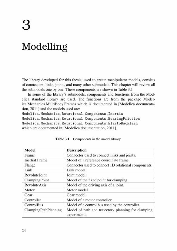
The library developed for this thesis, used to create manipulator models, consistsof connectors, links, joints, and many other submodels. This chapter will review allthe submodels one by one. These components are shown in Table 3.1

In some of the library’s submodels, components and functions from the Mod-elica standard library are used. The functions are from the package Model-ica.Mechanics.MultiBody.Frames which is documented in [Modelica documenta-tion, 2011] and the models used are:Modelica.Mechanics.Rotational.Components.InertiaModelica.Mechanics.Rotational.Components.BearingFrictionModelica.Mechanics.Rotational.Components.ElastoBacklashwhich are documented in [Modelica documentation, 2011].

Table 3.1 Components in the model library.

Model DescriptionFrame Connector used to connect links and joints.Inertial Frame Model of a reference coordinate frame.Flange Connector used to connect 1D rotational components.Link Link model.RevoluteJoint Joint model.ClampingPoint Model of the fixed point for clamping.RevoluteAxis Model of the driving axis of a joint.Motor Motor model.Gear Gear model.Controller Model of a motor controller.ControlBus Model of a control bus used by the controller.ClampingPathPlanning Model of path and trajectory planning for clamping

experiments.

24

3.1 Overview

3.1 Overview

As described in Section 2.1, coordinate frames attached to each link of the robot areused to describe the robot’s kinematics. Due to the nature of the Modelica languageand its use of connectors, our models have one frame (connector) at each end ofboth the link models and the joint models. Figure 3.1 illustrates a visualization ofan example model setup with the connection points between the frames in the links,joints, and the surrounding environment.

Figure 3.1 Example of manipulator structure with connection points.

Connections 1a, 2a, and 3a in Figure 3.1 are the connections between the endof a link and the beginning of next joint. Connections 1b, 2b, and 3b are the con-nections between the end of a joint and the beginning of next link. Connection 0is the connection between the beginning of the first link of the manipulator and theground (inertial frame). Connection 4 is the connection between the end of the lastlink and the clamping device. Each joint has an axis with subcomponents to drive itand to model the dynamics. The structure of an axis is visualized in Figure 3.2.

25

Chapter 3. Modelling

Figure 3.2 Structure of an axis model (real world robots don’t dont usually includea speed sensor but instead derives the angle).

The motor model is used to pass a torque input to the inertia model, whichcomputes the angular acceleration of the motor caused by the torque input. Tomodel the dynamics of the joint, submodels of friction, backlash, and elasticity(elastoBacklash models both backlash and elasticity) are used. A gear model isconnected at the end of the axis to translate motor rotation into joint rotation. Aspeed sensor and an angle sensor measure the angular velocity and position of themotor flange and pass the values to a control bus. The control bus is a connector thatcan be connected to a regulator to pass variables between the joint and the regulator.All of the axis models are described in more detail in Section 3.8.

3.2 Frame (connector)

Some points of the manipulator need to be connected by frames that describe theposition and orientation of a specific section of the manipulator and update saidpositions and orientations according to the kinematics and dynamics of the system.These points are essentially:

• The fixed points, i.e., the inertial frame and the fixed point representing theclamped end.

• The beginning and end of each link.

• The joints.

Each joint actually has two frames with equal positions. One frame that is equal,both in position and orientation, to the previous frame (most often the end of theprevious link) and one that is connected to the next link and is able to rotate around

26

3.3 Inertial Frame

a certain axis. Further, the frames handle the force and torque transmission betweendifferent parts of the robot. For source code, see Appendix A.1.

3.3 Inertial Frame

The inertial frame represents the point where the first link of the manipulator, thebase, is connected to the ground. This is the reference frame for expressing mostof the length vectors and positions for setting up the overall manipulator model andclamping point. This model consists of an instance of the connector Frame, whichhas fixed position and fixed rotation. For source code, see Appendix A.2.

3.4 Flange (connector)

The flange is used to connect components with one degree of freedom. The modelholds two variables, one for angle (rotational) and one for torque. This connectoris used to link the axis components, which only rotate with one degree of freedom,with respect to each other. For source code, see Appendix A.3.

3.5 Link

The link model consists of two frames, representing the end points of the link, sep-arated by a length vector. In order for Modelica to properly simulate the links, care-fully specified starting values for the velocity, angular velocity, and position are re-quired. The backwards part of the Newton-Euler equations specified in Section 2.4is used to model the link’s force and torque. However, the forward recursion is notneeded as the frame model contains information about the frame’s orientation andposition. Finding ωi, αi, and ac,i is easy using the features of the Modelica languageby specifying the correct relationships between derivatives of variables. Using theNewton-Euler equations for each link, it is possible to compute the cut force andtorque, which is then transmitted using the frames.

The frame that is referred to as frame i in the equations from Section 2.4 isattached to the side of the link that is closest to the base of the manipulator [Sponget al., 2005, p. 219]. In our model, the calculations are therefore performed withrespect to the first frame of the link, which is named frame_beg in the source codein Appendix A.4. The link model takes the parameters specified in Table 3.2

3.6 Joint

The joint model comprises a revolute joint and a revolute axis model and connectsthem to each other. These models are described in the following two sections.

27


Table 3.2 Parameters for the link model.

Parameter Unit Descriptionl m length vectorcm m vector from the first frame to the center of masswidth m width (and height) of the link, for animationI kgm2 inertia matrixm kg mass

Parameters for the revolute joint model and for the revolute axis model arepassed directly to this model. For parameter specification, see the sections for revo-lute joint and revolute axis models, respectively.

3.7 Revolute Joint

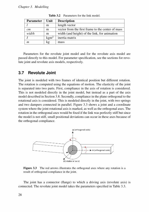
The joint is modeled with two frames of identical position but different rotation.The rotation is computed using the equations of motion. The elasticity of the jointis separated into two parts. First, compliance in the axis of rotation is considered.This is not modeled directly in the joint model, but instead as a part of the axismodel described in Section 3.8. Secondly, compliance in the plane orthogonal to therotational axis is considered. This is modeled directly in the joint, with two springsand two dampers connected in parallel. Figure 3.3 shows a joint and a coordinatesystem where the joint rotational axis is marked, as well as the orthogonal axes. Therotation in the orthogonal axes would be fixed if the link was perfectly stiff but sincethe model is not stiff, small positional deviations can occur in these axes because ofthe orthogonal compliance.

Figure 3.3 The red arrows illustrates the orthogonal axes where any rotation is aresult of orthogonal compliance in the joint.

The joint has a connector (flange) to which a driving axis (revolute axis) isconnected. The revolute joint model takes the parameters specified in Table 3.3.

28

3.8 Revolute Axis

Table 3.3 Parameters for the revolute joint model.

Parameter Unit Descriptionn − rotational axisc_orth Nm/rad rotational spring constant for orthogonal complianced_orth Nms/rad rotational damping constant for orthogonal compliance

3.8 Revolute Axis

The structure of the axis is described in Figure 3.2. This section reviews the parts— i.e., motor, inertia, friction, elasticity, backlash, gear, sensors, and control bus —in more detail. The revolute axis model connects to a revolute joint via a connector(flange).

MotorThe motor model is very simple. It takes a torque input to set the torque of the motorflange, which is connected to the next component of the axis. Thus, no detailedmodelling of the motor dynamics is included.

InertiaThe inertia model used in the axis is from Modelica’s Mechanics library,Modelica.Mechanics.Rotational.Components.Inertia [Modelica docu-mentation, 2011]. Given a parameter with the moment of inertia value, it uses thetorque from the motor to compute a resulting angular acceleration.

FrictionIn the revolute axis, the friction model is from Modelica’s Mechanics library,Modelica.Mechanics.rotational.Components.BearingFriction [Model-ica documentation, 2011]. It takes a table of values for the friction torque, coupled todifferent rotational velocities, and makes a linear interpolation of the values, whichare then used for the friction modelling. The user is able to provide a value for thepeak friction experienced when in stationarity. The friction torque is defined as:

τ f riction = kω−m, if ω < 0τ f riction = kω +m, if ω > 0|τ f riction| ≤ p ·m, if w = 0

(3.1)

where τ f riction is the friction torque, ω is the angular velocity of the axis, p is thepeak friction value, and k and m are constants. A graph corresponding to this defi-nition can be seen in Figure 3.4, compare this to Figure 2.4.

29


Figure 3.4 Friction torque in the axis.

Elasticity and BacklashThe model for elasticity and backlash is from Modelica’s Mechanics library,Modelica.Mechanics.Rotational.Components.ElastoBacklash [Modelicadocumentation, 2011]. This model takes a spring constant and a damping constantas parameters as well as an angle for the backlash and then uses Hooke’s law todescribe elasticity. The spring and the damper are connected in parallel and are thenconnected to the backlash in series, as illustrated in Figure 3.5.

Figure 3.5 Elasticity and backlash in the axis.

30

3.8 Revolute Axis

Table 3.4 The variables of control bus.

Parameter DescriptionmotorVelocity Measurement input to the controller.motorAngle Measurement input to the controller.angle_ref Reference to the controller.velocity_ref Reference to the controller.motorTorque Signal from the controller.

GearThis model describes a gear with ratio g and consists of two flanges with the fol-lowing relationships:

τarm = gτmotor (3.2)gφarm = φmotor. (3.3)

The dynamics of the gearbox, like backlash and elasticity, are not modeled here butare connected in series, as illustrated in Figure 3.2. The gear model consists of twoflanges where the first flange is connected to the chain of axis components and thesecond flange is connected to the axis flange. The axis flange is the connector thatthen will be connected to the joint flange, as described in Section 3.7.

Sensors and Control BusEvery instance of an axis has a control bus, an angle sensor, and a speed sensor. Thecontrol bus is a connector that holds all the variables used by the controller. Theseare described in Table 3.4. For the control bus source code, see Appendix A.10.

The two control bus variables motor angle and motor velocity are used asreference signals to the controller. They get their values from the angle sen-sor and the speed sensor in the axis, which are connected to the motor flange.The angle sensor and the speed sensor are from Modelica’s Sensor library,Modelica.Mechanics.Rotational.Sensors [Modelica documentation, 2011].

ParametersThe revolute axis model takes the parameters defined in Table 3.5.

Friction Table The friction table is an N × 2 matrix where angular velocity isentered in the left column and the corresponding friction torque is entered in thesecond column. The number of rows, N, can be any integer > 1 depending on howmuch data that are provided by the user. This matrix is then used in the frictionmodel to define a function—a first-order polynomial—that describes the relationbetween the angular velocity and the friction torque. A linear interpolation is per-formed and a first-order polynomial is fitted to the input data. As an example, the

31


Table 3.5 Parameters for the revolute axis model.

Parameter Unit Descriptionc Nm/rad rotational spring constantd Nms/rad rotational damping constantb rad backlashgearRatio − gear ratioinertia kgm2 inertia (one dimension)tau_pos − friction tablef riction_peak − friction peakbreaksOn − (boolean) true if the axis should be fixed

friction table matrix (1 32 5

)represents a friction torque value of 3 Nm at angular velocity 1 rad/s and 5 Nm atangular velocity 2 rad/s, respectively. The first-order polynomial corresponding tothis table is τ f riction = 2ω +1, for ω ≥ 0.

3.9 Clamping Device

The clamping device is modeled as a stiff spring that is connected to the end ofthe manipulator. Every deviation of the manipulator end effector, in position or ori-entation, from the clamped point is responded to with a large opposing force pro-portional to the deviation. This model, with compliance, was chosen to capture theimperfections of the clamping of the manipulator. The spring and damper constantsin this model are matrices so it is possible to change the compliance in a single di-rection if desiered. There are two types of elasticity and damping represented by thematrices; both translational and rotational. So the stiffness parameters can be set ineach direction and around each axis. The clamping point model takes the parametersspecified in Table 3.6.

3.10 Controller

Modelica blocks, as described in Section 2.9, are used to represent the differentparts of the controller, which are illustrated in the block diagram in Figure 2.6. Theblocks are then connected to each other according to the control diagram, and thereference, feedback, and output blocks are connected to the axis control bus of thejoint that should be controlled.

32

3.11 Path Planning

Table 3.6 Parameters for the clamping device.

Parameter Unit Descriptionc_lin N/m spring constant for clamping point complianced_lin Ns/m damping constant for clamping point compliancec_rot Nm/rad spring constant for clamping point complianced_rot Nms/rad damping constant for clamping point compliance

Table 3.7 Parameters for the controller.

Parameter Unit Descriptionkp − gain of position controllerks − gain of speed controllerT s s time constant of integrator of speed controllerratio − gear ratio of the joint that is controlled

This controller uses feedback from the motor side, i.e., motor angle and motorvelocity instead of joint angle and joint velocity. However, the reference signalsare for the arm side, i.e., joint angle and joint velocity. Consequently, the referencesignals are multiplied with the gear ratio of the gear box in the joint, to get thedesired behavior. The reason for using measurements from the motor side is thatmost industrial robots have sensors on the motor side and not on the arm side.

The controller model takes the parameters specified in Table 3.7. For sourcecode, see Appendix A.12.

3.11 Path Planning

To be able to simulate clamping experiments, suitable reference signals for the con-troller are needed. The path planning model handles this by using the Modelicablock Modelica.Blocks.Sources.KinematicPTP2 [Modelica documentation,2011]. This block generates output signals for moving as fast as possible from astart position to an end position, given kinematic constraints. The constraints to bepassed are maximum velocity and maximum acceleration of the joint. The outputsare angle reference, velocity reference, and acceleration reference.

By combining five KinematicPTP2 blocks, the path planning model outputs ref-erence signals for moving back and forth, to a given maximum/minimum angle.Figures 3.6 and 3.7 show examples of two angle reference signals and velocity ref-erence signals plotted over 15 seconds. The parameters used in the example areshown in Table 3.8.

33


Table 3.8 Parameters used in Figures 3.6 and 3.7.

Parameter ValueMaximum/minimum angle π/20 (≈ 0.157 rad)Maximum velocity 0.2 rad/sMaximum acceleration 0.5 rad/s²

Figure 3.6 Example of angle reference plotted against time.

Figure 3.7 Example of velocity reference plotted against time.

For source code, see Appendix A.14.

34

3.12 Wrist

3.12 Wrist

The wrist model has three flange connectors for external driving axes. These flangesdrive the wrist according to the transmission matrix, as described in Section 2.2, thatis given as a parameter when initializing the wrist. The compliance of the wrist isnot modeled here but is taken care of by the external axes connected to the flanges.The wrist model only takes the parameter transmission, describing the variable Gin Equations (2.1)-(2.2). This model of the wrist does not include any orthogonalcompliance, for more on wrist modelling, see [Niglis and Öberg, 2015].

35

4Results

This chapter provides results of simulations performed with manipulator modelsbuilt with the model library discussed in the previous chapter. Focus lies on modelvalidation and the effects of different dynamic behavior like friction, backlash, andjoint compliance on the resulting joint/axis dynamics. During the simulations, re-sults from all six joints of the robot have been considered. However, for readabilityreasons, all clamping curves are not presented here but results have been singledout to those who demonstrate the dynamic effects in the most visible way for therespective case.

4.1 Dymola and JModelica.org

Running the Modelica simulations can be done on many different platforms. Thislibrary has been tested in both Dymola [Dymola, 2017] and JModelica.org [Jmodel-ica.org, 2017] with similar results. An example of clamping curves from two identi-cal model set-ups simulated in both Dymola and Jmodelica.org can be seen in Figure4.1. In these simulations, JModelica.org is using the CVode solver [CVODE] andDymola is using the Dassl solver [Petszold, 1982]. The results in this example areclose to identical, and has been in all comparisons between the two platforms.

The results presented in this chapter all come from simulations performed inDymola. The reason for using Dymola is mainly that it has a more accessible userinterface and animation features, which makes it easier to evaluate simulation re-sults.

36

4.2 ABB IRB140 Experiments

Figure 4.1 Clamping curves from simulations done with Dymola and Jmodel-ica.org.

4.2 ABB IRB140 Experiments

The results in this chapter are solely from simulations done with a model of ABB’srobot IRB140 [ABB IRB140 data, 2017]. The effects of parameters representingdifferent dynamic behaviour have been examined and at the end of the chapter, sim-ulation results will be compared to measured data from real clamping experimentswith IRB140. Figure 4.2 shows a picture of the robot.

37

Chapter 4. Results

Figure 4.2 ABB IRB140 manipulator in the Robotics lab, shared by the Depart-ment of Automatic Control and Department of Computer Science at Lund University.

Figure 4.3 shows clamping curves from experimental data provided by Cog-nibotics. The character of these curves will be further examined and compared tosimulated results in Section 4.10. For now, they only serve as an example of thecharacteristics of clamping curves.

The data visualized in the plots in Figure 4.3 come from experiments where theend-effector of the IRB140 was clamped to a fixed object and load is applied by therobots own motors, as described in Section 2.3.

38

4.3 Simulation Setup

Figure 4.3 Clamping curves for the six axes of IRB140. Experimental data pro-vided by Cognibotics.


The simulations in Sections 4.4-4.9 were performed using the clamping configura-tion shown in Figure 4.4 (full drawn lines). All joints have individual controllersand have been given a certain angle reference. The Modelica code for this simu-lation setup is shown in Listing 4.1. The six links, the three base joints, and the

39

Chapter 4. Results

wrist are all initiated individually with parameters defining the characteristics. Forthe links the parameters describe the dimensions and the weight and for the jointsand wrist they define the elasticity, friction, gear ratio and inertia. After also initiat-ing controllers, an inertial frame, path planners and a clamping device everything isconnected in the equation section and ready for simulation.

model IRB140Demoimport C = Modelica.Constants;

InertialFrame IF "Inertial frame";

// Defining the links with length , width and mass.Link base(l={0,0.1 ,0},width=0.05 ,m=20);Link link1a(l={0.07 , 0, 0},width=0.05 ,m=10);Link link1b(l={0, 0.252 ,0},width=0.05 ,m=20);Link link2(l={0,0.360 ,0},width=0.05 ,m=20);Link link3(l={0.38 ,0,0},width=0.05 ,m=23);Link link4(l={0.065 ,0,0},width=0.05 ,m=5);

// Defining all joints except for the wrist joints.Joint joint1(n={0,1,0},c=10,d=5,b=0.01 ,c_orth=10000000 , tau_pos=

[0,0.1;1,0.3],gearRatio=104.4,inertia=0.014);Joint joint2(n={0,0,1},c=20,d=2,b=0.01 ,c_orth=10000000 , tau_pos=

[0,0.1;1,0.3],gearRatio=104.4,inertia=0.014);Joint joint3(n={0,0,1},c=40,d=2,b=0.01 ,c_orth=10000000 , tau_pos=

[0,0.1;1,0.3],gearRatio=100.74 ,inertia=0.014);

// Defining the wrist with transmission matrix.Wrist wrist(transmission = {{110.0 /6649.0, 0, 0},{71.0/(22.0*6649.0/110.0*207675 .0 /3190.0), 3190.0 /207675.0 , 0},{(71.0*243360 .0*22.0+207675 .0 /3190.0*64.0*22.0*4147.0)/(22.0*4147.0*22.0*6649.0/110.0*207675 .0 /3190.0*486720 .0 /7975.0),243360 .0/(4147.0*207675 .0 /3190.0*486720 .0 /7975.0),7975.0 /486720 .0}});

// Defining the axes that power the wrist.RevoluteAxis axis4(c=0.4,d=0.1 ,b=0.01 ,tau_pos=[0,0.1;1,0.3],

gearRatio=1,inertia=0.014);RevoluteAxis axis5(c=2.5,d=0.5 ,b=0.01 ,tau_pos=[0,0.1;1,0.3],

gearRatio=1,inertia=0.014);RevoluteAxis axis6(c=0.8,d=0.1 ,b=0.01 ,tau_pos=[0,0.1;1,0.3],

gearRatio=1,inertia=0.014);

// Defining the controller.Controller controller1(

kp=0.008 ,ks=0.01 ,Ts=0.11 ,ratio = 104.4);

Controller controller2(kp=0.008 ,ks=0.01 ,

40


Ts=0.12 ,ratio = 104.4);

Controller controller3(kp=0.008 ,ks=0.01 ,Ts=0.28 ,ratio = 100.74);




// Defining a path for the controller.ClampingPathPlanning path(q_pos=C.pi/10, qd_max=0.4,qdd_max=0.8);ClampingPathPlanning path2(q_pos=C.pi/6,qd_max=0.4,qdd_max=0.8);

// Defining the stiffnes of the clamped end.ClampingDevice cp(c_rot=20000000*identity(3),

c_lin=20000000*identity(3));

equation//Chain of connections from inertial frame through all links//and joints all the way to the clamped end.connect(IF.frame_end , base.frame_beg);connect(base.frame_end , joint1.frame_beg);connect(joint1.frame_end , link1a.frame_beg);connect(link1a.frame_end , link1b.frame_beg);connect(link1b.frame_end , joint2.frame_beg);connect(joint2.frame_end , link2.frame_beg);connect(link2.frame_end , joint3.frame_beg);connect(joint3.frame_end , link3.frame_beg);connect(link3.frame_end , wrist.frame_beg);connect(wrist.frame_end , link4.frame_beg);connect(link4.frame_end , cp.frame);

// Connecting the controller to the control bus of the joint and//to the angle reference and velocity reference//of the path planner.connect(controller1.controlBus.angle_ref , path.q);connect(controller1.controlBus.velocity_ref , path.qd);connect(controller1.controlBus , joint1.controlBus);

connect(controller2.controlBus.angle_ref , path.q);

41

Chapter 4. Results

connect(controller2.controlBus.velocity_ref , path.qd);connect(controller2.controlBus , joint2.controlBus);

connect(controller3.controlBus.angle_ref , path.q);connect(controller3.controlBus.velocity_ref , path.qd);connect(controller3.controlBus , joint3.controlBus);

connect(controller4.controlBus.angle_ref , path2.q);connect(controller4.controlBus.velocity_ref , path2.qd);connect(controller4.controlBus , axis4.controlBus);



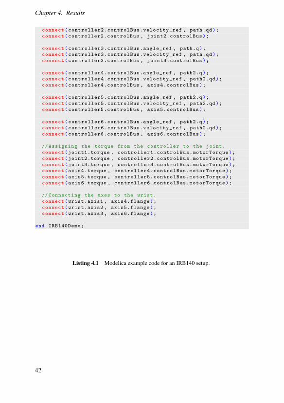
// Assigning the torque from the controller to the joint.connect(joint1.torque , controller1.controlBus.motorTorque);connect(joint2.torque , controller2.controlBus.motorTorque);connect(joint3.torque , controller3.controlBus.motorTorque);connect(axis4.torque , controller4.controlBus.motorTorque);connect(axis5.torque , controller5.controlBus.motorTorque);connect(axis6.torque , controller6.controlBus.motorTorque);

// Connecting the axes to the wrist.connect(wrist.axis1 , axis4.flange);connect(wrist.axis2 , axis5.flange);connect(wrist.axis3 , axis6.flange);

end IRB140Demo;

Listing 4.1 Modelica example code for an IRB140 setup.

42

4.4 Joint Compliance

Figure 4.4 Drawing of IRB140 with geometry specifications [ABB Robotics,2017]. The positioning of the manipulator in this drawing is used in the followingsimulations.

4.4 Joint Compliance

First, the compliance along the direction of the rotational axis of the joint will beexamined. Orthogonal compliance will be examined later in Section 4.7. The com-pliance in the axis is modeled by a rotational spring and a damper as described inSection 2.5. The relationship between the torque, angular displacement, and angularvelocity is described by the equation

τ = cθ +dω

where τ is the torque, θ is the angular displacement, and ω is the angular velocity.In Figure 4.5, two different values for c are used, while the rest of the simulationsettings are identical. No orthogonal compliance is modeled in these simulationsand the compliance in the clamped end is small.

43

Chapter 4. Results

Figure 4.5 Clamping curves from two simulations with different spring constants.The black dotted lines are the corresponding linear regressions.

The two resulting clamping curves in Figure 4.5 demonstrate the effect of chang-ing the spring constant. When doubling the value of the spring constant c, the slopeof the clamping curve gets roughly twice as steep. The increase in steepness indi-cates that more torque is needed for the same rotation, which is an expected effectwhen having a stiffer spring. When performing a linear regression, the resultinglines are on the form τ = β0 +β1θ where the interesting part is β1, representing theslope of the line. For the orange curve, β1 = 9.2389 which is close to the expectedvalue of 10. For the blue curve, β1 = 17.0773 which differ a bit from the expectedvalue of 20. However, it demonstrates that a doubling of the spring constant resultsin that the slope gets close to twice as steep, which is a good result.

Figure 4.6 shows the effects of varying the damping constant d. When increasingthe damping constant, the angular velocity decreases, especially around the turningpoints at minimum/maximum motor angle. This too is expected behaviour, sincea higher damping constant is supposed to slow down the motion. The speed ofthe motor of axis 2 in these simulations are between 0 and 0.4 rad/s and the mostsignificant difference in speed of the two simulations occurs when the motor angleis in the range of 0.1 radians from the turning points.

44

4.5 Friction

Figure 4.6 Clamping curves from two simulations with different damping con-stants.

4.5 Friction

The friction model used in the simulations describes the friction torque as a functionof the angular velocity of the axis. This function is limited to be on the form ofa polynomial of degree one as described in (3.1). Figures 4.7 and 4.8 show thedifference in clamping curves when alternating the value for k and m, respectively.

45

Chapter 4. Results

Figure 4.7 Clamping curves from two simulations with different values of m in thefriction equation (3.1).

Figure 4.8 Clamping curves from two simulations with different values of k in thefriction equation (3.1).

46

4.5 Friction

Figure 4.7 shows the effects of a higher value of m. The vertical segments ofthe curve increases much, which means that the motor is standing still for a longerperiod of time. This is an expected result, since a higher value of m means that thefriction torque function has a higher value at zero velocity and consequently, moretorque is needed to transition from static friction into kinetic friction.

Figure 4.8 demonstrates the effects of a higher value of k. Also here, the curveshows expected characteristics. A higher value of k should result in higher frictionat all velocities, and more torque needed for the motor to drive. This is indicatedby the wider hysteresis of the curve with a higher value of k. Notice an importantdifference to Figure 4.5 — here, the motor eventually reaches the same position forboth settings, whereas the curves in Figure 4.5 shows that a higher spring constantleads to a different end position. Friction does not influence the final position.

The model also has a parameter for peak friction. If the value of this parameteris 6= 1, it changes the size of the friction torque at zero velocity, and the frictiontorque is in that case determined by (3.1). Figure 4.9 shows the effects of using apeak-value 6= 1.

Figure 4.9 Clamping curves from two simulations with different peak values inthe friction equation (3.1).

The effects of a higher peak friction are similar to those of a higher value of m. Thatis, a bigger segment of the curve is vertical which means that the motor is in static

47

Chapter 4. Results

mode for a longer time. It is a sensible result, since the friction torque around zerovelocity is higher in both cases.

4.6 Backlash

The backlash parameter b determines the size of the backlash in radians. Figure 4.10illustrates the effect of backlash on the clamping curve. The two curves are resultsfrom two simulations with equal parameters and configuration, except one of themhas a backlash of 0.01 radians in joint 2 and the other has no backlash.

Figure 4.10 Clamping curves showing the effect of backlash.

The appearance of the orange curve indicates that backlash in the model has thedesired effect. When the torque is close to zero, an effect of the backlash is that themotor can rotate without much resistance. This makes the steepness of the clampingcurve lower in a certain interval. In the plot above this is observed between motorangles of 0.01 and -0.05 radians. Figure 4.11 and 4.12 shows the effects of differentvalues for the backlash parameter.

48

4.6 Backlash

Figure 4.11 Clamping curves from two simulations with different backlash size.

Figure 4.12 Clamping curves from two simulations with different backlash size.

The effects on the clamping curves in Figure 4.12 when alternating the size ofthe backlash are as expected; a bigger backlash leads to a bigger segment of the

49

Chapter 4. Results

curve with lower steepness. In Figure 4.11, however, the size of the backlash doesnot seem to affect the apperance of the clamping curve much. Fore more analysis ofthis observation, see the discussion in Section 5.

4.7 Orthogonal Compliance

Each joint has a spring parameter, c_orth, that determines the amount of orthog-onal compliance. Figure 4.13 shows the effects on the clamping curves when com-paring two simulations with equal settings, except one of them has orthogonal com-pliance and one of them has not.

Figure 4.13 The effects of adding orthogonal compliance. Spring parameterc_orth = 108 Nm/rad for joints 1, 2, and 3.

There is definitely an observable effect of adding orthogonal compliance to thejoints, and the clamping curves for all six joints were influenced in the simulations.As expected, the effects are very different depending on the configuration of therobot and the geometric relation between the rotational axes of the joints. The effectsof joint 2, whose behavior is illustrated in Figure 4.13, are both a small decrease ofthe slope of the curve but also an increase of the motor rotation. When adding morecompliance to a system, both of these effects seem reasonable.

50

4.7 Orthogonal Compliance

Figure 4.14 Clamping curves from two simulations with different values of theorthogonal compliance spring parameter.

Figures 4.14 and 4.15 show the clamping curves for different values of c_orth.

Figure 4.15 Clamping curves from two simulations with different values of theorthogonal compliance spring parameter.

51

Chapter 4. Results

These clamping curves indicate a similar behavior as for the compliance in therotational axis of the joint. However, in this case it is not the compliance of the jointitself that affects its clamping curve, but instead the compliance of the other jointsof the manipulator. This will be discussed more in Chapter 5.

4.8 Compliance in the Clamped End

When the end-effector of the robot is clamped to a fixed object, there will always bea small amount of compliance in the clamping point. In the model for the clampingdevice, the compliance is modeled by a spring and the amount of compliance isdetermined by the spring constant c. In this experiment both the rotational springand the linear spring is set to the same value c. Figure 4.16 shows the effects onthe clamping curve when alternating the spring constant. In the simulation with thespring parameter, c= 2 ·107 N/m (Nm/rad for the rotational spring), the end effectordeviated 0.15 mm from the starting position and in the other simulation it moved0.29 mm from the starting position. These are small differences but they seem tohave a considerable influence on the appearance of the clamping curves. The effectsare not trivial to interpret from the clamping curves, but a small change in maximumand minimum motor angle can be observed. The slope and the width of hysteresisof the curve, however, do not seem to be affected.

52

4.9 Clamping Configuration

Figure 4.16 Clamping curves from two simulations with different values of theclamping device compliance.

4.9 Clamping Configuration

The results of the clamping simulations appear to be quite sensitive to the configu-ration of the manipulator, i.e., what start position is used. Figure 4.17 shows simula-tions with equal parameters but different configurations. Clamping configuration 1represents the configuration in Figure 4.4 with dashed lines and configuration 2represents the solid drawn configuration in Figure 4.4.

53

Chapter 4. Results

Figure 4.17 Clamping curves from two simulations with different configurations.

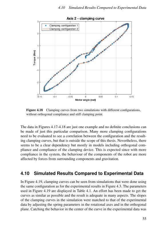
The data in Figure 4.17 was generated with a model that included orthogonal com-pliance of the joints. Figure 4.18 show clamping curves from the same configura-tions but without orthogonal compliance of the joint and with a much stiffer clamp-ing device.

54

4.10 Simulated Results Compared to Experimental Data

Figure 4.18 Clamping curves from two simulations with different configurations,without orthogonal compliance and stiff clamping point.

The data in Figures 4.17-4.18 are just one example and no definite conclusions canbe made of just this particular comparison. Many more clamping configurationsneed to be evaluated to see a correlation between the configuration and the result-ing clamping curves, but that is outside the scope of this thesis. Nevertheless, thereseems to be a clear dependency but mostly in models including orthogonal com-pliance and compliance of the clamping device. This is expected since with morecompliance in the system, the behaviour of the components of the robot are moreaffected by forces from surrounding components and gravitation.


In Figure 4.19, clamping curves can be seen from simulations that were done usingthe same configuration as for the experimental results in Figure 4.3. The parametersused in Figure 4.19 are displayed in Table 4.1. An effort has been made to get thecurves as similar as possible and the result is adequate in many aspects. The slopesof the clamping curves in the simulation were matched to that of the experimentaldata by adjusting the spring parameters in the rotational axes and in the orthogonalplane. Catching the behavior in the center of the curve in the experimental data was

55

Chapter 4. Results

done by adjusting the backlash in the simulation. Getting the desired behavior atthe turning points was accomplished by tweaking the friction parameters. The over-all behavior from the experimental data has been reconstructed in the simulations.However, the non-linear behaviour of axis 3 and 5 in the experimental curves couldnot be captured using a linear elasticity model.

Figure 4.19 Clamping curves from a simulated clamping experiment. Comparewith the experimental data in Figure 4.3.

56


Table 4.1 Parameters used for obtaining the results in Figure 4.19

joint Parameter Value1 c 71 d 0.51 b 0.041 tau_pos [0,0.1; 1,0.4]1 f riction_peak 21 c_orth 5000000001 d_orth 1002 c 8.22 d 0.582 b 0.012 tau_pos [0,0.12; 1,0.2]2 f riction_peak 12 c_orth 100000002 d_orth 103 c 103 d 0.0013 b 0.013 tau_pos [0,0.1; 1,0.9]3 f riction_peak 13 c_orth 300000003 d_orth 104 c 0.324 d 0.0054 b 0.014 tau_pos [0,0.05; 1,0.055]4 f riction_peak 1.75 c 1.45 d 0.0015 b 0.055 tau_pos [0,0.08; 1,0.085]5 f riction_peak 16 c 0.166 d 0.0016 b 0.046 tau_pos [0,0.05; 1,0.06]6 f riction_peak 1.4

57

5Discussion andConclusions

In this chapter, the results from the previous chapter are discussed and used to drawconclusions about the modelling and the clamping experiments.

5.1 Simulation Results

The joint compliance spring parameter (Section 4.4) is largely what determines theslope of the clamping curve, since this is the parameter which determines how muchtorque is needed from the motor for the gearbox to be deformed. However, whenobserving the results from the orthogonal compliance of the joints (Section 4.7), thesame type of effect can be seen, since looser springs for the orthogonal complianceallows the links to move when the other joints are excited. So there appears to bemany parameters that can affect the clamping curves in similar ways, which makesit hard to identify what parameter that gave rise to one particular effect. Compare theeffect of the joint compliance spring parameter in Figure 4.5 with the effect of theorthogonal compliance spring parameter in Figure 4.14, they both affect the slope ofthe curve in a similar way and introduce an uncertainty about what observed effectsare connected to what parameters.

This uncertainty is also present when observing the width of the hysteresis of thecurve. Considering the effect of the joint compliance damper parameter in Figure4.6, it is easy to see that a higher value for the damping parameter adds to thewidth of the hysteresis of the curve. The same behaviour can be seen when lookingat Figure 4.8, where the effect of the value of k in the friction equation has beenexamined. These two parameters appear to give the same effect on the clampingcurve. This should come as no surprise though, as they basically achieve the samething in this simplified friction model. They both give more torque when the axis ismoving faster.

The effects of the backlash component is not straightforward to analyze. Firstly,the inclusion of it in the model can be seen very clearly in the clamping curve (Fig-

58

5.2 Friction

ure 4.10). An interesting observation is that just a small backlash seems to havea significant effect on the curve (Figure 4.10) and adding more backlash does notseem to affect the curve proportionally (Figure 4.11). This is true up to a certainpoint, because adding a wider backlash gap shows up on the curve (Figure 4.12).The compliance of the clamped end also seem to affect the apperance of the back-lash.

The effects of the clamping configuration are significant, but not surprising asthe configuration affects the length of the levers and the way that gravity affects thelinks.

5.2 Friction

When modeling friction torque as a function of angular velocity, it is certainly a lim-itation and a rough simplification to only use a first-order polynomial. There are alot of dynamic behaviour that will not be captured in this linear model. For instance,the behavior during the short time interval when an axis in the robot leaves a sta-tionary state and starts to rotate is typically not well described by a linear function.The friction characteristics are also known to vary with temperature. This wouldmean that there could be a substantial difference between running a cold robot thathas been idle for a while and a robot that is already warmed up. This, and a lot moreon the topic of friction in robot models, can be found in [Niglis and Öberg, 2015].

During the clamping experiments, the manipulator is stationary and the jointswill move very slowy. This led us to believe that additional emphasis should beput on the friction effects for angular velocities close to zero. In the work with themodel library in this thesis, an attempt was made to implement a more advancedmodel. The focus of that implementation was on the friction effects when the angu-lar velocity is close to zero. In that model, the torque at low velocities was describedusing a polynomial of higher degree. However, due to time limitations, a workingmodel was never completed within this project.

5.3 Link Elasticity

The compliance in the joints does not fully describe the manipulators elastic behav-ior. Another source of compliance could be the elasticity in the links. It could beinteresting to develop the link models in the library to also model the link stiffnessand the dynamic behavior connected to the stiffness. This is a complicated subjectand it was not possible to cover it in the scope of this thesis. If the link elasticitywas modeled, it could possibly have some impact on the results of the simulationsin this thesis, but since the load used in clamping experiments are quite low, one canargue that the effects of link elasticity would be quite low. More on the topic of linkelasticity in robots can be found in [Nilsson et al., 2013].

59

Chapter 5. Discussion and Conclusions

5.4 Joint Types

In the model library developed for this thesis, only revolute type joints are included.In robot manipulators, those are not the only type of joints that are common. An-other often seen joint type is the prismatic joint. Prismatic joints are joints that allowlinear relative motion between two links [Spong et al., 2005]. Models for such jointswere not developed for this thesis because of time limitations. However, if therehad been more time available, it would had been interesting to develop such modelssince there are a lot of industrial robots that uses prismatic joints, or a combinationof revolute and prismatic.

5.5 Future Work

The work of this thesis has been centred mostly around the development of theModelica models and not as much around using the models for simulations, exceptfor in model validation purposes. The results are from only one type of robot, ABB’sIRB140, and it would be interesting to set up models for other type of robots toevaluate the results. However, the model library was not built with the IRB140 inconsideration and there is nothing indicating it would work worse for other robottypes. It would also be interesting to extend the model library to be able to modelparallel-bar robots, like the ABB IRB2400 robot [ABB IRB2400 data, 2017], whichis currently not possible.

As discussed previously in this chapter, the friction models of the robot couldbe more advanced and that would possibly have an impact on the results, especiallyaround the lowest motor velocities in the simulations. To improve the friction modelwould be of high priority if more work should be done with the models.

5.6 Conclusions

The overall purpose of this thesis was to establish models, to investigate how thedynamical effects of the manipulator affect the clamping curves in clamping exper-iments, and to validate them. The effects of compliance in the joint (both along theaxis of rotation and in the plane orthogonal to this axis), the effects of backlash,the effects of compliance in the clamping device and the effects of the clampingconfiguration have all been studied and the models work well in many aspects. Theeffects of the friction, however, could be investigated further with a more advancedfriction model (as discussed in Section 5.2).

The goal was to create a library that could be used to model and simulate manydifferent types of manipulators within the delimitations set up prior to project start.All models built with six degrees of freedom or less have simulated successfully.The modularity aspect of the library was also discussed in the introduction to thisthesis. This has been considered throughout the work with the model library and

60

5.6 Conclusions

all setups of manipulator models are made with submodels that can be reused fordifferent types of manipulators.

61

Bibliography

Declarative modelling, 2016. http : / / www . simulistics . com / tour /declarative.htm.

Modelica documentation, 2011. http : / / www . maplesoft . com /documentation_center/online_manuals/modelica/Modelica.html.

ABB IRB140 data, 2017. Abb robotics website. http : / / new . abb . com /products/robotics/industrial-robots/irb-140/irb-140-data.

ABB IRB2400 data, 2017. Abb robotics website. http : / / new . abb . com /products/robotics/industrial-robots/irb-2400/irb-2400-data.

Asada, H. H. (2005). Introduciton to robotics. Massachusetts Institute of Technol-ogy.

Bagdad, W. S. (2008). Mechatronics. 4th ed. Technical Publications Pune.Cognibotics, 2017. Cognitotics.com. http://cognibotics.com.CVODE. Cvode. http://computation.llnl.gov/projects/sundials/

cvode.Dymola, 2017. Dymola website. https://www.3ds.com/products-services/

catia/products/dymola.Newton-Euler approach, 2016. Dynamic model of robots: newton-euler approach.

http : / / www . diag . uniroma1 . it / ~deluca / rob2 _ en / 06 _NewtonEulerDynamics.pdf.

World Robotics 2016. Executive summary world robotics 2016 industrial robots.http://www.ifr.org/fileadmin/user_upload/downloads/World_Robotics/2016/Executive_Summary_WR_Industrial_Robots_2016.pdf.

KHK Stock Gears, 2016. Gear backlash. http : / / khkgears . net / gear -knowledge/gear-technical-reference/gear-backlash/.

Khan Academy, 2017. Hooke’s law. https : / / www . khanacademy . org /science / physics / work - and - energy / hookes - law / a / what - is -hookes-law.

62

Bibliography

ABB Robotics, 2017. Irb140 technical data. http://new.abb.com/products/robotics/sv/industrirobotar/irb-140/data.

Jmodelica.org, 2017. Jmodelica website. https://www.http://jmodelica.org/.

Modelica language specification, 2014. Language specification. https://www.modelica.org/documents/ModelicaSpec33Revision1.pdf. Version 3.3.

Lewotsky, Kristin. Understanding Backlash and Stiction. http : / / www .motioncontrolonline.org/content-detail.cfm/Motion-Control-Technical - Features / Understanding - Backlash - and - Stiction /content_id/310.

Niglis, A. and P. Öberg (2015). Modelling High-Fidelity Robot Dynamics. MA the-sis. Linköping University.

Nilsson, K. (2012). “Metod och system för bestämning av minst en egenskap hos enmanipulator”. Patent SE 536708. [Online; accessed 18-Feb-2017]. URL: http://was.prv.se/spd/patent?p1=-V9wPAbAQXN7eM42P9NdVA.

Nilsson, K., A. Nilsson, M. Haage, B. Olofsson, A. Robertsson, and O. Sörnmo(2013). “Metod och system för bestämning av åtminstone en egenskap hos enmanipulator”. Patent SE 537534. [Online; accessed 18-Feb-2017]. URL: http://was.prv.se/spd/patent?p1=8MTFKl_ArpZ7eM42P9NdVA.

Petszold, L. (1982). A description of dassl: a differential/algebraic system solver.Ross, L. T., S. W. Fardo, J. W. Masterson, and R. L. Towers (2011). Robotics:

Theory and Industrial Applications. 2nd ed. Goodheart-Willcox.Simulink. Simulation and model-based design. https://se.mathworks.com/

products/simulink.html.Spong, M. W., S. Hutchinson, and M. Vidyasagar (2005). Robot Modeling and Con-

trol. John Wiley & Sons, Inc.

63

AModelica Models

A.1 Frame

connector Frame

import SI = Modelica.SIunits;

SI.Position r[3]"Position of frame , expressed in inertial frame.";

Modelica.Mechanics.MultiBody.Frames.Orientation R"Orientation object of frame.";

flow SI.Force f[3];flow SI.Torque t[3];

end Frame;

Listing A.1 Modelica code for the connector Frame.

A.2 InertialFrame

model InertialFrameimport Modelica.Mechanics.MultiBody.Frames;

Frame frame_end;equation

frame_end.R = Frames.nullRotation()"Defining null rotation of InertialFrame.";

frame_end.r = zeros(3) "Defining the position of origin.";

Connections.root(frame_end.R)"Defining root node in virtual connection graph.";

end InertialFrame;

Listing A.2 Modelica code for the model InertialFrame.

64

A.3 Flange

A.3 Flange

connector Flange


SI.Angle phi;flow SI.Torque tau;

end Flange;// Derived from Modelica.Mechanics.Rotational.Interfaces.Flange_a

Listing A.3 Modelica code for the model Flange.

A.4 Link

model Link "Stiff link model."

import Modelica.Mechanics.MultiBody.Frames;import SI = Modelica.SIunits;

parameter SI.Length l[3] "Length vector expressed in inertialframe , resolved in frame_beg.";

parameter SI.Length cm[3] = l/2"Vector from frame_beg to center of mass.";

parameter Real width = 0.1 "Only used for animation.";

Frame frame_beg;Frame frame_end;

SI.Velocity v[3](start={0,0,0});SI.Acceleration a[3];

SI.AngularVelocity w[3](start={0,0,0});SI.AngularAcceleration z[3];

parameter SI.Inertia I[3,3] = 0.01*identity(3)"Inertia matrix.";

parameter SI.Mass m= 10 "Mass of link.";

constant SI.Acceleration g[3] = {0, -9.82 , 0}"Gravity acceleration vector.";

Modelica.Mechanics.MultiBody.Visualizers.Advanced.Shape shape1(shapeType="box",color={255,0,0},length=Modelica.Math.Vectors.norm(l),width=width ,

65

Appendix A. Modelica Models

height=width ,lengthDirection=l/Modelica.Math.Vectors.length(l),widthDirection={0,1,0},r_shape=zeros(3),r=frame_beg.r ,R=frame_beg.R) "Animation";

equation// Velocity and acceleration of link center of gravity.v = der(frame_beg.r + Frames.resolve1(frame_beg.R ,cm));a = der(v);

// Angular velocity and acceleration of frame_beg.Modelica.Mechanics.MultiBody.Frames.angularVelocity2(frame_beg.R) = w;z = der(w);

//Force and torque equations , Newton -Euler backward recursion.frame_beg.f = -frame_end.f +

m*(Frames.resolve2(frame_beg.R ,a - g));frame_beg.t = -frame_end.t +cross(cm, frame_beg.f) +cross(-frame_end.f , -l + cm) +I*z + cross(w, I*w);

// Defining potential root and non-breakable branch.Connections.potentialRoot(frame_beg.R);Connections.branch(frame_beg.R ,frame_end.R);

//Link does not bend , rotation is equal.frame_end.R = frame_beg.R;

// Definition of positional relationship between endpoints.frame_end.r = frame_beg.r + Frames.resolve1(frame_beg.R , l);

end Link;

Listing A.4 Modelica code for the model Link.

A.5 Joint

model Joint "Joint model with actuator , modelled withcompliance , friction , and backlash."import SI = Modelica.SIunits;import C = Modelica.Constants;

// Parameters to pass to RevoluteJoint and Revolute Axis.parameter Modelica.Mechanics.MultiBody.Types.Axis n = {0,1,0};parameter Real c_orth = 1000000;parameter Real d_orth = 30;

parameter SI.RotationalSpringConstant c = 50;parameter SI.RotationalDampingConstant d = 10;parameter SI.Angle b = 0.01;parameter Real gearRatio = 140;

66

A.6 RevoluteJoint

parameter Real tau_pos[: ,2] = [0, 1; 1, 1.1];parameter Real friction_peak = 1;parameter Real inertia = 0.01;parameter Boolean breaksOn = false;

Frame frame_beg;Frame frame_end;Modelica.Blocks.Interfaces.RealInput torque;ControlBus controlBus;

RevoluteJoint revoluteJoint(n=n,c_orth=c_orth ,d_orth=d_orth);

RevoluteAxis revoluteAxis(c=c,d=d,b=b,gearRatio=gearRatio ,tau_pos=tau_pos ,friction_peak = friction_peak ,inertia=inertia ,breaksOn=breaksOn);

equationconnect(revoluteJoint.frame_beg , frame_beg);connect(revoluteJoint.frame_end , frame_end);connect(revoluteJoint.flange , revoluteAxis.flange);connect(revoluteAxis.torque , torque);connect(revoluteAxis.controlBus , controlBus);

end Joint;

Listing A.5 Modelica code for the model Joint.

A.6 RevoluteJoint

model RevoluteJoint "Revolute joint with orthogonal compliancemodelled by spring and damper in parallel."

import SI = Modelica.SIunits;import C = Modelica.Constants;import Modelica.Mechanics.MultiBody.Frames;

parameter Modelica.Mechanics.MultiBody.Types.Axis n"Rotational axis of joint.";

parameter Real c_orth"Spring constant for orthogonal compliance.";

parameter Real d_orth"Damping constant for orthogonal compliance.";

67


SI.Angle q(start = 0) "Rotation angle , starting at zero.";SI.AngularVelocity w(start = 0, fixed = true)

"Angular velocity , starting at zero.";

Real orthRotAxis1[3] "Axis orthogonal to n.";Real orthRotAxis2[3] "Axis orthogonal to n and orthRotAxis1.";

SI.Angle orth1(start = 0)"Angular displacement in first orthogonal axis.";

SI.AngularVelocity wo1(start = 0, fixed = true);

SI.Angle orth2(start = 0)"Angular displacement in second orthogonal axis.";

SI.AngularVelocity wo2(start = 0, fixed = true);


SI.Torque orthTorque1 "Torque in orthRotAxis1.";SI.Torque orthTorque2 "Torque in orthRotAxis2.";

Flange flange "Flange for connecting external driving axis.";

protectedFrames.Orientation R_rel

"Relative rotation of frame_beg and frame_end.";

equation(orthRotAxis1 , orthRotAxis2)= getOrthVectors(n) "Make orthRotAxis1 and orthRotAxis2orthogonal to each other and to n.";

// Define relationship between angle and angular velocity.w = der(q);wo1 = der(orth1);wo2 = der(orth2);

frame_end.r = frame_beg.r;

-frame_end.t*n = flange.tau"Torque in rotational axis , from external actuator.";

// Torque in orthogonal rotational axis.frame_end.t*orthRotAxis1 = orthTorque1;frame_end.t*orthRotAxis2 = orthTorque2;

//Hooke 's law.orthTorque1 = c_orth*orth1 + d_orth*wo1;orthTorque2 = c_orth*orth2 + d_orth*wo2;

flange.phi = q;

// Relative rotation of joint in rotational axis and// rotation in orthogonal axes because of compliance.

68

A.7 RevoluteAxis

R_rel = Frames.axesRotations({1,2,3},q*n + orth1*orthRotAxis1 +orth2*orthRotAxis2 ,w*n + wo1*orthRotAxis1 + wo2*orthRotAxis2);Frames.absoluteRotation(frame_beg.R , R_rel) = frame_end.R;

//Force and torque transfer.Frames.resolve1(R_rel ,frame_end.f) = -frame_beg.f;Frames.resolve1(R_rel ,frame_end.t) = -frame_beg.t;

end RevoluteJoint;

Listing A.6 Modelica code for the model RevoluteJoint.

A.7 RevoluteAxis

model RevoluteAxis "Driving axis with gearbox containingelasticity , backlash , and friction. Sensors for speed andangle are avaibable for controller."

import SI = Modelica.SIunits;import Modelica.Mechanics.Rotational;

parameter SI.RotationalSpringConstant c = 50"Spring constant for gearbox elasticity.";

parameter SI.RotationalDampingConstant d = 10"Damper constant for gearbox elasticity.";

parameter SI.Angle b = 0.001 "Backlash of gearbox (rad).";parameter Real gearRatio = 1 "Gear ratio of gearbox.";parameter Real inertia = 0.01 "Inertia of motor.";parameter Real tau_pos[: ,2] = [0, 1; 1, 1.1]

"Friction values.";parameter Real friction_peak = 1 "Friction peak in w = 0.";parameter Boolean breaksOn = false "Break parameter.";

Motor motor(breaksOn = breaksOn);Rotational.Components.Inertia I( J=inertia);Rotational.Components.BearingFriction bearingFriction(tau_pos=tau_pos , useSupport=false , peak = friction_peak);Rotational.Components.ElastoBacklash backlash(c = c, d = d, b = b);Gear gear(ratio = gearRatio);

Rotational.Sensors.AngleSensor angleSensor;Rotational.Sensors.SpeedSensor speedSensor;Modelica.Blocks.Interfaces.RealInput torque;

Flange flange;ControlBus controlBus;

equationconnect(motor.flange , I.flange_a);connect(I.flange_b , bearingFriction.flange_a);connect(bearingFriction.flange_b , backlash.flange_a);connect(backlash.flange_b , gear.flange_beg);

69


connect(gear.flange_end , flange);

connect(motor.flange , angleSensor.flange);connect(motor.flange , speedSensor.flange);connect(motor.torque , torque);

connect(angleSensor.phi , controlBus.motorAngle);connect(speedSensor.w , controlBus.motorVelocity);

end RevoluteAxis;

Listing A.7 Modelica code for the model RevoluteAxis.

A.8 Motor

model Motor "Motor model with breaks."import SI = Modelica.SIunits;

parameter Boolean breaksOn = false;import C = Modelica.Constants;

SI.Angle phi;Flange flange;

Modelica.Blocks.Interfaces.RealInput torque"Input torque to motor.";

equationif breaksOn then

torque = 0;flange.phi = 0;phi = 0;

elseflange.tau = -torque;flange.phi = phi;

end if;end Motor;

Listing A.8 Modelica code for the model Motor.

A.9 Gear

model Gear "Gear model for perfect gear."


Flange flange_beg;Flange flange_end;

parameter Real ratio = 1;

70

A.10 ControlBus

equationflange_beg.phi = flange_end.phi*ratio;flange_beg.tau*ratio = -flange_end.tau;

end Gear;

Listing A.9 Modelica code for the model Gear.

A.10 ControlBus

expandable connector ControlBus "Connector used forcommunications between sensors and controller."import SI = Modelica.SIunits;

SI.AngularVelocity motorVelocity;SI.Angle motorAngle;

SI.Angle angle_ref;SI.AngularVelocity velocity_ref;

SI.Torque motorTorque;

end ControlBus;

Listing A.10 Modelica code for the model ControlBus.

A.11 ClampingPoint

model ClampingDevice "Clamping modelled by spring and damper inparallel , one for spatial displacement and one for rotational."

import SI = Modelica.SIunits;import Modelica.Mechanics.MultiBody.Frames;

Frame frame;

parameter Real[3,3] c_lin = 9001*identity(3)"Spring constants for linear springs.";

parameter Real[3,3] d_lin = 9001*identity(3)"Damper constants for linear dampers.";

parameter Real[3,3] c_rot = 9001*identity(3)"Spring constants for rotational springs.";

parameter Real[3,3] d_rot = 9001*identity(3)"Damper constants for rotational dampers.";

SI.Position dr[3](start = {0, 0, 0}, fixed = true)"Spatial displacement vector.";

SI.Velocity v[3];

SI.Angle q[3](start = {0, 0, 0}, fixed = true)

71


"Angular displacement vector";SI.AngularVelocity w[3];

equation// Defining relationships between position and velocity.der(frame.r) = v;der(dr) = v;der(q) = w;

//Hooke 's law.frame.t = c_rot*q + d_rot*w;frame.f = c_lin*dr + d_lin*v;Frames.angularVelocity2(frame.R) = w;

end ClampingDevice;

Listing A.11 Modelica code for the model ClampingPoint.

A.12 Controller

model Controller

import SI = Modelica.SIunits;import Modelica.Blocks.Math;import Modelica.Blocks.Continuous;

parameter Real kp=10 "Gain of position controller";parameter Real ks=1 "Gain of speed controller";parameter SI.Time Ts=0.01

"Time constant of integrator of speed controller";parameter Real ratio=1 "Gear ratio of gearbox";

Math.Gain gain1(k=ratio);Continuous.PI PI(k=ks , T=Ts,initType=Modelica.Blocks.Types.Init.InitialOutput);Math.Feedback feedback1;Math.Gain P(k=kp);Math.Add3 add3(k3=-1);Math.Gain gain2(k=ratio);

ControlBus controlBus;

equationconnect(gain1.y , feedback1.u1);connect(feedback1.y , P.u);connect(P.y , add3.u2);connect(gain2.y , add3.u1);connect(add3.y , PI.u);connect(gain2.u , controlBus.velocity_ref);connect(gain1.u , controlBus.angle_ref);connect(feedback1.u2 , controlBus.motorAngle);connect(add3.u3 , controlBus.motorVelocity);connect(PI.y , controlBus.motorTorque);

72

A.13 Wrist

// Derived from// MultiBody.Examples.Systems.RobotR3.Components.Controller

end Controller;

Listing A.12 Modelica code for the model Controller.

A.13 Wrist

model Wrist "Wrist model with transmission matrix , externalactuators are requierd to move it."

import SI = Modelica.SIunits;import Modelica.Mechanics.MultiBody.Frames;


parameter Real transmission[3,3] "Transmission matrix.";parameter Real controlJoint = 1

"(1 = joint 4, 2 = joint 5, 3 = joint 6)";

Flange axis1;Flange axis2;Flange axis3;

// Rotation angle vector and angular velocity vector.SI.Angle q[3](start = {0,0,0});SI.AngularVelocity w[3](start = {0,0,0}, fixed = true);

protectedFrames.Orientation R_rel;

equationw = der(q);

frame_end.r = frame_beg.r;

transpose(transmission)*(-frame_end.t) ={axis1.tau , axis2.tau , axis3.tau};

transmission*{axis1.phi , axis2.phi , axis3.phi} = q;

// Rotation of wrist.R_rel = Frames.axesRotations({1,2,3}, q, w);frame_end.R = Frames.absoluteRotation(frame_beg.R , R_rel);

//Force and torque transfer.frame_beg.f = -Frames.resolve1(R_rel , frame_end.f);frame_beg.t = -Frames.resolve1(R_rel , frame_end.t);

end Wrist;

Listing A.13 Modelica code for the model Wrist.

73


A.14 ClampingPathPlanning

block ClampingPathPlanning "Block for generating referencesignals (angle and velocity) for clamping experiments."

import SI = Modelica.SIunits;import C = Modelica.Constants;import Modelica.Blocks.Sources;

Modelica.Blocks.Interfaces.RealOutput q;Modelica.Blocks.Interfaces.RealOutput qd;

parameter Real q_pos = C.pi /20 "maximum/minimum angle";parameter Real qd_max = 0.2 "maximum velocity";parameter Real qdd_max = 0.5 "maximum acceleration";

Sources.KinematicPTP2 path1(q_end={q_pos},qd_max={qd_max},qdd_max={qdd_max},startTime=0,q_begin={0});

Sources.KinematicPTP2 path2(q_end={-q_pos},qd_max={qd_max},qdd_max={qdd_max},startTime=3,q_begin={q_pos});

Sources.KinematicPTP2 path3(q_end={q_pos},qd_max={qd_max},qdd_max={qdd_max},startTime=6,q_begin={-q_pos});

Sources.KinematicPTP2 path4(q_end={-q_pos},qd_max={qd_max},qdd_max={qdd_max},startTime=9,q_begin={q_pos});

Sources.KinematicPTP2 path5(q_end={q_pos},qd_max={qd_max},qdd_max={qdd_max},startTime=12,q_begin={-q_pos});

equation

74

A.15 getOrthVectors

q = if time < 3 then path1.q[1]else if (time >= 3 and time < 6) then path2.q[1]else if (time >= 6 and time < 9) then path3.q[1]else if (time >= 9 and time < 12) then path4.q[1]else if (time >= 12 and time < 15) then path5.q[1]else q_pos;

qd = if time < 3 then path1.qd[1]else if (time >= 3 and time < 6) then path2.qd[1]else if (time >= 6 and time < 9) then path3.qd[1]else if (time >= 9 and time < 12) then path4.qd[1]else if (time >= 12 and time < 15) then path5.qd[1]else 0;

end ClampingPathPlanning;

Listing A.14 Modelica code for the model ClampingPathPlanning.

A.15 getOrthVectors

function getOrthVectors "Function returns two arbitrary vectorsorthogonal to eachother and to input vector."input Real n[3];output Real u[3];output Real v[3];

algorithm//First vector u, is computed using crossproduct with input//vector , n, and an arbitrary vector not parallel to n.if n[1] == 0 then

u :=cross({1,0,0}, n);elseif n[2] == 0 then

u :=cross({0,1,0}, n);else

u :=cross({0,0,1}, n);end if;

u :=Modelica.Math.Vectors.normalize(u);v :=cross( n, u) "v is computed by crossing n with u.";

end getOrthVectors;

Listing A.15 Modelica code for the function getOrthVectors.

75

Document name

Date of issue

Document Number

Author(s) Supervisor

Sponsoring organization

Title and subtitle

Abstract

Keywords

Classification system and/or index terms (if any)

Supplementary bibliographical information

ISSN and key title ISBN

Language Number of pages Recipient’s notes

Security classification

hfodudwlyh 0rghov iru 6hoi &doleudwlqj...

Documents