hidden heritability due to heterogeneity across seven

ARTICLESDOI: 10.1038/s41562-017-0195-1

© 2017 Macmillan Publishers Limited, part of Springer Nature. All rights reserved.

1 Department of Sociology/Nuffield College, University of Oxford, Oxford OX1 3UQ, UK. 2 School of Environmental and Rural Science, University of New England, Armidale, NSW 2351, Australia. 3 Department of Sociology/Interuniversity Center for Social Science Theory and Methodology, University of Groningen, Groningen 9712 TG, The Netherlands. 4 Department of Epidemiology, University Medical Center Groningen, University of Groningen, Groningen 9700 RB, The Netherlands. 5 Erasmus University Rotterdam Institute for Behavior and Biology, Erasmus School of Economics, Rotterdam 3062 PA, The Netherlands. 6 Department of Complex Trait Genetics, University Amsterdam, Amsterdam, The Netherlands. 7 Institute of Molecular Biosciences, The University of Queensland, Brisbane, QLD 4072, Australia. 8 Department of Psychology, University of Illinois at Urbana-Champaign, Champaign, IL 61820-9998, USA. 9 Department of Medical Epidemiology and Biostatistics, Karolinska Institutet, PO Box 281, Stockholm SE-171 77, Sweden. 10 Estonian Genome Center, University of Tartu, 51010 Tartu, Estonia. 11 Quantitative Genetics Laboratory, Queensland Institute of Medical Research Berghofer Medical Research Institute, Brisbane, QLD 4029, Australia. 12 Department of Computational Biology, University of Lausanne, Lausanne CH-1015, Switzerland. *e-mail: [email protected]

Genome-wide association studies (GWAS) dominate genetic discovery, and meta-analyses of such studies are based on diverse data sources that span vast historical time periods

and populations1. The proportion of phenotypic variance accounted for by single-nucleotide polymorphisms (SNPs) that reach genome-wide significance, and the polygenic scores constructed from all SNPs using GWAS results, however, represent only a frac-tion of heritability estimates derived from twin and other whole-genome studies2,3.

To understand this disparity, it is essential to explain three cen-tral ways of measuring heritability (see Box 1 for detailed defini-tions). First, narrow-sense heritability stems from family-based studies and often twin research (h2

family) and produces the highest heritability estimates. These studies have demonstrated a genetic basis for anthropometric traits such as height and body mass index (BMI), but also behavioural phenotypes such as educational attain-ment and human reproductive behaviour (that is, number of chil-dren ever born (NEB) and age at first birth (AFB))4–6. For instance, a recent meta-analysis of twin studies from 1958–20124 estimated heritability as 52% for educational attainment (n = 24,484 twin pairs) and 31% for reproductive traits (n = 28,819 twin pairs).

GWAS heritability estimates (h2GWAS) estimate the proportion

of phenotypic variance accounted for by genetic variants known to be robustly associated with the phenotype of interest and

produce the lowest estimates. The polygenic score from a recent meta-GWAS of educational attainment with over 300,000 partici-pants explains around 4% of the variance5 with another GWAS for AFB explaining only 1%6.

Yang et al.7,8 argued that most genetic effects are too small to be reliably detected in GWAS of current sample sizes and proposed an alternative approach: whole-genome restricted maximum like-lihood estimation (GREML) performed by genome-wide complex trait analysis (GCTA) software. This third measure is often referred to as SNP- or chip-based heritability (denoted by h2

SNP), and is the proportion of phenotypic variance explained by additive genetic variance jointly estimated from all common variants on standard GWAS chips. These estimates are typically between h2

family and h2GWAS

estimates. Contrary to the low h2GWAS estimates of between 1 and

4% for these phenotypes, the SNP heritability has been estimated as 22% for educational attainment, 15% for AFB and 10% for NEB9,10.

This stark discrepancy in heritability estimates has spawned debates about ‘missing heritability’ (the difference between h2

GWAS and h2

family) and ‘hidden heritability’ (the difference between h2GWAS

and h2SNP) (for full definitions see Box 1)2,3,11–13. ‘Missing heritability’

has been linked to fundamental differences in study designs between family and whole-genome studies2, non-additive genetic effects11,12 and inflated estimates from twin studies due to shared environmen-tal factors14. Empirical evidence for either of these reasons is scarce.

Hidden heritability due to heterogeneity across seven populationsFelix C. Tropf1*, S. Hong Lee2, Renske M. Verweij3, Gert Stulp! !3, Peter J. van der Most! !4, Ronald de Vlaming! !5,6, Andrew Bakshi7, Daniel A. Briley8, Charles Rahal1, Robert Hellpap1, Anastasia N. Iliadou9, Tõnu Esko10, Andres Metspalu10, Sarah E. Medland11, Nicholas G. Martin11, Nicola Barban1, Harold Snieder4, Matthew R. Robinson7,12 and Melinda C. Mills1

Meta-analyses of genome-wide association studies, which dominate genetic discovery, are based on data from diverse his-torical time periods and populations. Genetic scores derived from genome-wide association studies explain only a fraction of the heritability estimates obtained from whole-genome studies on single populations, known as the ‘hidden heritability’ puz-zle. Using seven sampling populations (n!= !35,062), we test whether hidden heritability is attributed to heterogeneity across sampling populations and time, showing that estimates are substantially smaller across populations compared with within populations. We show that the hidden heritability varies substantially: from zero for height to 20% for body mass index, 37% for education, 40% for age at first birth and up to 75% for number of children. Simulations demonstrate that our results are more likely to reflect heterogeneity in phenotypic measurement or gene–environment interactions than genetic heterogeneity. These findings have substantial implications for genetic discovery, suggesting that large homogenous datasets are required for behavioural phenotypes and that gene–environment interaction may be a central challenge for genetic discovery.

NATURE HUMAN BEHAVIOUR | www.nature.com/nathumbehav

mailto:[email protected]

http://orcid.org/0000-0003-0173-5554

http://orcid.org/0000-0001-8450-3518

http://orcid.org/0000-0001-6416-6067

http://www.nature.com/nathumbehav

© 2017 Macmillan Publishers Limited, part of Springer Nature. All rights reserved. © 2017 Macmillan Publishers Limited, part of Springer Nature. All rights reserved.

ARTICLES NATURE HUMAN BEHAVIOUR

A recent investigation on height and BMI, however, demonstrated that the inclusion of rare genetic variants can increase the herita-bility estimate based on whole-genome methods13. The underlying reason for the discrepancy of ‘hidden heritability’ between h2

SNP and h2

GWAS estimates is less well understood15.Here, we interrogate the common assumption underlying

GWAS meta-analyses—that genetic effects are ‘universal’ across environments. The large GWAS meta-analyses required to detect SNP associations consist of a wide array of samples across histori-cal periods and countries, representing heterogeneous populations subject to diverse environmental influences. Heterogeneity across environments can emerge for different reasons, such as differences in population structure, genotype or phenotype measurement, het-erogeneous imputation quality across sampling populations or sen-sitivity of the phenotype to environmental change. Demographic research has shown that education and reproductive behaviour are strongly modified by environmental changes such as female educational expansion or the introduction of effective contracep-tion16. If genetic effects are not universal but rather heterogeneous across populations, heritability estimates from GWAS meta-analy-ses should produce weaker signals and we would witness a reduc-tion in both the discovery rate and the variance explained by SNPs across populations17.

We conducted a mega-analysis using whole-genome methods, which entailed pooling all cohorts to estimate genetic relatedness not only within, but also across populations. We used models based on GREML estimation8 with primary data from seven pooled sam-pling populations. This allowed us to estimate the average common

SNP-based heritability (h2SNP) between and within environments.

We subsequently applied gene–environment interaction models, adding a within-population matrix to estimate the average SNP-based heritability within populations in our data and decomposed the variance explanation of common SNPs within and between sampling populations and birth cohorts8,18. If SNP-based heritabil-ity was significantly higher within than across environments, we would conclude that this was evidence for hidden heritability due to heterogeneity across the sample population or cohort. We applied a gene × sampling population (G× P) model when stratifying by sam-pling populations, a gene × demographic birth cohort (G× C) model when stratifying by birth cohorts born before or after the strong fertility postponement during the twentieth century (see Methods and Fig. 1) and a gene × sampling population × demographic birth cohort (G× P× C) model when stratifying by both (see Methods for details). We defined the various genetic variance components of the models explicitly, and will refer to hSNP

2 as the sum of all genetic effects relative to the phenotypic variance within the respective model specification. We quantified the hidden heritability due to heterogeneity as the discrepancy between hSNP

2 from the baseline model and hSNP

2 from the interaction models.Our approach allowed us to decompose average heritability levels

across historical cohorts and countries into a genetic component that was either ‘universal’ across all environments or ‘environmentally specific’, enabling us to test whether the same genes explain variance in the phenotype to the same extent in different geographical (coun-try) and historical (birth cohort) environments. To test for alter-native explanations for heterogeneity across sampling populations,

Box 1 | Definitions of heritability

HeritabilityHeritability is the proportion of the phenotypic variance accounted for by genetic effects and narrow sense heritability refers to the additive genetic variance component41,42. There are several ways to estimate heritability. First, the highest and prominent estimates are derived from family-based studies (h2

family), such as twin studies, where, typically, the genetic resemblance between relatives is mapped to phenotypic similarity, taking unique and shared environment effects into account. Under several assumptions, estimates of h2

family ought to reflect only additive genetic effects. A second method is the proportion accounted for by genetic variants known to be robustly associated with the phenotype of interest, derived from GWAS (h2

GWAS). This measure tends to produce the lowest levels. Finally, there is the proportion of phenotypic variance jointly accounted for by all variants on standard GWAS chips. This is sometimes referred to as the SNP- or chip-based heritability (h2

SNP). Typically, h2SNP is substantially larger than

h2GWAS and provides an ‘upper level estimate’ of the genetic effects

that could be identified with a well-powered GWAS. The h2GWAS

increases in tandem with GWAS sample sizes and is expected to approach h2

SNP asymptotically under the assumption that the phenotype of interest is homogeneous in its genetic architecture across different environments.

Missing heritabilityThe gap between h2

family and h2GWAS is referred to as ‘missing

heritability’2. Potential reasons for missing heritability are, for example, non-additive genetic effects (although empirical evidence on this is scarce)6,11, large effects of rare variants13 and potentially inflated estimates from twin studies due to shared environmental factors14. The missing heritability is commonly defined as the sum of the still-missing and hidden heritability, which we define below3.

Still-missing heritabilityYang et al.7 argued that most genetic effects are too small to be reliably detected in GWAS of current sample sizes, which is why they proposed the whole-genome restricted maximum likelihood estimation performed by GCTA software8. Studies applying these whole-genome methods typically produce estimates that lie between twin studies and polygenic scores: h2

GWAS < h2SNP < h2

family. The discrepancy h2

SNP < h2family has been referred to as ‘still-missing

heritability’3. A stylized fact is that for many traits the still-missing heritability is roughly equal to h2

SNP (ref. 43). It is generally assumed that by genotyping rarer and structural variants, the still-missing heritability decreases as the denser arrays increase h2

SNP (ref. 13).

Hidden heritabilitySince we expect to be able to almost fully capture h2

SNP in the long run, the discrepancy between h2

SNP and h2GWAS is sometimes

referred to as ‘hidden heritability’3. The current study is mainly interested in the question of how h2

SNP changes, depending on whether we examine differences within or between populations. Here, we focus on hidden heritability as the genetic variation due to heterogeneity that cannot possibly be explained by SNP associations based on meta-analyses of multiple populations. Since h2

GWAS is usually inferred from meta-analyses that include multiple populations, heterogeneity in genetic effects on a phenotype between these populations could deflate h2

GWAS and would also deflate h2

SNP, which is typically obtained within single populations. Within a single design, we therefore demonstrate how one estimate of h2 depends on population heterogeneity. Missing heritability is thus commonly defined as the sum of the still-missing and hidden heritability3. As indicated, the hidden portion decreases as sample sizes grow and the still-missing portion decreases with denser forms of genotyping.




ARTICLESNATURE HUMAN BEHAVIOUR

such as genotyping error, we conducted a series of simulation stud-ies to evaluate the role of gene–environment interaction in contrast with alternative explanations (for details and results, see the Discussion and Methods). A recent study used bivariate GREML models to investigate genetic heterogeneity in height and BMI between two populations in the United States and Europe, providing evidence for homogeneity in both phenotypes19. We expected negli-gible gene–environment interaction for these anthropometric traits and compared the findings for these homogeneous phenotypes with those from behavioural phenotypes (education and human repro-ductive behaviour) using the same modelling framework.

ResultsSNP-based heritability across model specifications by pheno-types. When we ignored environmental differences, h2

SNP in the standard GREML model was significant for all phenotypes, but at different levels (Fig. 2; see Supplementary Tables 1–5 for full model estimates). For height, h2

SNP was estimated as 0.40 (s.e.m. = 0.01), meaning that 40% of the variance in height could be attributed to common additive genetic effects. h2

SNP was smaller for BMI (0.17; s.e.m.: 0.01) and years of education (0.16; s.e.m. = 0.01) and low for both reproductive behaviour outcomes—NEB (0.03; s.e.m. = 0.01) and AFB (0.08; s.e.m. = 0.02).

More importantly, however, for our question, h2SNP in all phe-

notypes increased when we included stratified genetic relatedness matrices (GRMs) in addition to the baseline GRM (for example, yielding the G× C model when stratifying by birth cohorts, the G× P model when stratifying by sampling populations and the G× P× C model when stratifying by both). Particularly for the com-plex behavioural outcomes of education and reproductive behav-iour, the increase was substantial. For education, h2

SNP increased by 80% (up to 0.28; s.e.m. = 0.03) in the G× P× C model compared with the standard GREML model. For AFB, the increase was 60% (0.13; s.e.m. = 0.04) and for NEB it was as high as 342% (0.13; s.e.m. = 0.03). In contrast, the increase in the full G× P× C model was considerably smaller at 12% (0.44; s.e.m. = 0.03) for height and 30% (0.22; s.e.m. = 0.03) for BMI.

Best model by phenotype. Based on likelihood ratio tests, we iden-tified the best-fitting while parsimonious model (in Fig. 2 marked as BM; for full results see Supplementary Table 6). For height, the best-fitting model included no gene–environment interaction and therefore corroborated previous findings from the literature19.

For BMI and the reproductive phenotypes of AFB and NEB, the G× P specification showed the best model fit. This indicated signifi-cant heterogeneity interaction across sampling populations, while there was no evidence for heterogeneity by birth cohort. For BMI, additive SNP variance, which is effective between and within popu-lations (that is, the blue column in Fig. 2 that assumes it is effective across the defined environments or ‘universal’, respectively; σ σ∕G Y

2 2), explains 16% of the variance in the phenotype, and an additional 5% could be explained on average within populations (σ σ∕×G P Y

2 2; green column in Fig. 2). For AFB, around 6% of the variance could be explained by universal genetic effects while 7% were environ-mentally specific, and for NEB only 1% of the variance could be explained between populations and 12)% within them. Finally, for education, the best-fitting model (G× P× C) implies that both the sampling population and the birth cohort moderate genetic effects from the whole genome and that there were genetic effects unique to sampling populations within the defined birth cohorts. In contrast with reproductive behaviour, however, 12% of the over-all variance could still be explained by additive common genetic effects even between populations. Additionally, 2% of variance was explained within birth cohorts (σ σ∕×G C Y

2 2; red column in Fig. 2), 6% was explained within populations and 8% was unique within popu-lations and birth cohorts (σ σ∕× ×G P C Y

2 2; orange column in Fig. 2).

Quantifying ‘universal effects’ and ‘hidden heritability’ due to heterogeneity. Figure 3 visualizes the ‘universal effects’ or ratio for genetic variance captured by the normal GRM in the best-fitting model (that is, the blue column, σ σ∕G Y

2 2 in the model with the best fit) and the total hSNP

2 (that is, across all genetic components in the best-fitting model). It also shows in red the ‘hidden heritability’ due to heterogeneity (that is, the differences in total hSNP

2 between the best-fitting model and the baseline model, divided by the total hSNP

2 of the best-fitting model) for all phenotypes.

Figure 3 illustrates hidden heritability due to heterogeneity particularly for the complex phenotypes we are most interested in, namely education and the reproductive outcomes of AFB and NEB. For education, only 55% of hSNP

2 in the best-fitting model was ‘universal’ or effectively both within and between environments. A standard GREML model would only capture around 63% of hSNP

2 in the best-fitting model, resulting in 37% hidden heritability. For reproductive behaviour, this became even stronger. For NEB, only 6% of hSNP

2 in the best-fitting model was universal, with 75% hid-den heritability due to heterogeneity in the baseline model. For AFB, 45% of hSNP

2 was universal with around 40% of the hSNP2 hid-

den in the baseline model. In contrast, for height, the hSNP2 in the

best-fitting model was effectively between environments and there was no evidence for hidden heritability. For BMI, around 75% of hSNP

2 in the best-fitting model was effectively between and within environments (that is, universal). The standard GREML model for BMI thus captured 80% of hSNP

2 from the best-fitting model with 20% hidden heritability.

DiscussionUsing whole-genome data from seven populations, we demonstrate heterogeneity in genetic effects across populations and birth cohorts for educational attainment and human reproductive behaviour in a mega-analysis framework. Our findings imply substantial ‘hidden heritability’ due to heterogeneity for educational attainment (37%) and reproductive behaviour (40% for AFB and 75% for NEB) in the cohorts in this study. Comparative analysis with anthropometric traits (height and BMI) corroborates previous findings from whole-genome methods of a more homogeneous genetic architecture

23

25

27

29

1920 1940 1960 1980Birth year

Age

at fi

rst b

irth

(yea

rs)

CountryAustralia (estimated)EstoniaEstonia (estimated)NetherlandsSwedenUnited KingdomUnited States

Fig. 1 | Trends in mean AFB of women indicating environmental changes across cohorts (1903–1970) from the United States, United Kingdom, Sweden, the Netherlands, Estonia and Australia. Trends in the mean AFB of women are based on aggregated data obtained from the Human Fertility Database and Human Fertility Collection (for details see Supplementary Note 3). For Estonia, from 1962 onwards, we used the estimated AFB based on women older than 40. For Australia, no official data were available and the trends were estimated from the QIMR dataset and averaged for each decade.





of these phenotypes across environments (while for BMI, GWAS also find evidence for gene–environment interaction across birth cohorts in the Health and Retirement Study (HRS)20,21.

Our findings indicate that the lower predictive power of poly-genic scores from large GWAS compared with SNP-based herita-bility on single or very few populations partly reflects the fact that genetic effects are (to some extent) not universal but rather specific to data sources for these complex traits. Estimates are well in line with the 36–38% loss in polygenic score R2 across datasets reported for education17. They therefore demonstrate that the reference SNP-based heritability for the predictive power of polygenic scores obtained from the GWAS meta-analyses among several populations is smaller than SNP-based heritability obtained from single popu-lations. While the need for statistical power often still necessitates large-scale GWAS meta-analysis combining multiple and diverse data sources, our findings also suggest that large homogeneous data sources such as the UK Biobank, which contains data on around 500,000 genotyped individuals, may trigger genetic discovery for behavioural outcomes. However, it may be inaccurate to draw con-clusions or make predictions out of one discovery sample alone, since SNPs may have different effects in different samples, or the phenotype may reflect different behavioural aspects.

Complementary simulation studies corroborate the interpre-tation that our findings are mainly driven by gene–environment interaction in contrast with heterogeneity in residual environmen-tal variance—including measurement error—or genetic heteroge-neity (for example, the genotyping platform, genetic architecture or imputation quality) across the data sources we pooled (see Methods). When applying our models to simulated phenotypes without gene–environment interaction, but rather to different levels of heritability due to varying residual variance, we found

no systematic inflation of the G× P component in our models. Furthermore, we estimated both models, including and exclud-ing the causal 5,000 SNPs our simulations had been based on. When causal SNPs were removed, estimates were based on cor-related SNPs, which were in linkage disequilibrium. To the extent that the structure in the genetic data we used was heterogeneous across populations for the above reasons, we expect that our mod-els interpreted this heterogeneity as heterogeneous genetic effects resulting in hidden heritability. However, the results including and excluding causal SNPs were nearly identical, so we cannot expect heterogeneity to have driven our findings. In the total absence of gene–environment interaction, estimates showed a slight inflation in the G× P model (5%; see Figs 4 and 5 and Methods for details on all simulation studies). First, the substantial findings of hidden heritability between 40 and 75% for behavioural phenotypes largely exceeded this potential inflation, corresponding with simulations of a genetic correlation between 0.5 and 0.8 across populations for the behavioural phenotypes. Second, we conducted permuta-tion analyses, generating a random gene–environment interac-tion, not stratifying by population or birth cohorts. Here, we found no inflation for AFB by a randomly generated matrix included in the models (σ ×G P

2 0.000001; s.e.m. = 0.03; P = 0.50), nor for NEB (σ ×G P

2 0.003; s.e.m. = 0.02; P = 0.43) nor education (σ ×G P2 0.000001;

s.e.m. = 0.02, P = 0.50; not listed). It remains vital to conclude that although the estimates of hidden heritability provided in our study are in a single design—in contrast with comparing GWAS and whole-genome methods—estimates do not represent general-izable values of hidden heritability for these traits. The estimates might be slightly inflated and dependent on the number of cohorts combined for a study, as well as the respective level of heterogene-ity across them.

BM BM BM BM BM

Education AFB NEB BMI Height

GG×

CG×

P

G×P×

C GG×

CG×

P

G×P×

C GG×

CG×

P

G×P×

C GG×

CG×

P

G×P×

C GG×

CG×

P

G×P×

C

0.0

0.1

0.2

0.3

0.4

Model specification

SNP–

base

d ad

ditiv

e ge

netic

var

ianc

e co

mpo

nent

s

σ2G×P×C/σ2

P σ2G×P/σ2

P σ2G×C/σ2

P σ2G/σ2

P

Fig. 2 | Stacked bar charts of average between (σGG2) and within (σ σ σ× × × ×GG PP GG CC GG PP CC,

2 2 2 ) variance explanation by common SNPs estimated for height, BMI, education, AFB and NEB in four model specifications (G, G×P, G×C and G×P×C). The best model (BM) was based on likelihood ratio tests comparing the full model with one constraining the respective variance component to 0 (see Supplementary Table 6). σG

2/σP2 represents the proportion of observed

variance in the outcome associated with genetic variance across all environments, σ ×G P2 /σP

2 the proportion of observed variance in the outcomes associated with additional genetic variance within populations, σ ×G C

2 /σP2the proportion of observed variance associated with additional genetic variance

within demographic birth cohorts and σ σ∕× ×G P C P2 2 the proportion of observed variance associated with additional genetic variance within populations

and demographic birth cohorts. The model specifications G, G× P, G× C and G× P× C refer to the model specifications including the respective variance components as well as those of lower order (see Methods). For detailed results see Supplementary Tables 1–5.





In contrast with our expectations, we did not find any evidence for gene–environment interaction across birth cohorts for human reproductive behaviour. This is particularly surprising since across time there have been substantial environmental changes such as the introduction of effective contraception, social norms around the timing of childbearing and educational expansion—all factors that strongly modify reproductive behaviour16. In contrast, we found cohort-specific genetic effects on educational attainment. This con-tributes to solving the puzzle of missing heritability in educational attainment, since twin studies with higher heritability estimates are also conducted within homogeneous birth cohorts.

Our findings expose the challenges in detecting genetic vari-ants associated with human reproductive behaviour or other com-plex phenotypes in GWAS meta-analyses of multiple cohorts. First, SNP-based heritability within populations is comparably small and second, we found limited evidence that genetic effects underly-ing reproductive behaviour in one country predict the underlying behaviour in another. Our findings probably reflect the interrelated behavioural nature of reproduction and education, which appears to be more sensitive to cultural and societal heterogeneity than, for example, anthropometric traits such as height or BMI. It has also been shown that pleiotropic genes affecting AFB and schizophrenia have different effects across populations22. Recently, social scientists have made considerable efforts to integrate molecular genetics into their research5,6,10. When considering the highly socially and biolog-ically related phenotype of reproductive behaviour outcomes, envi-ronmental factors are critical in understanding how genetic factors are modified in relation to fecundity and infertility.

Our study has several important limitations. First, it is possible that heterogeneity in the phenotypic measures influenced the pat-terns we observed. While we found no evidence that our models interpreted changing relative environmental contributions to trait variation as gene–environment interaction, we cannot rule out the possibility that the trait definitions differed across environments. We consider this a minor issue for reproductive behaviour. While measures were not perfectly harmonized across birth cohorts (for example, some questionnaires explicitly asked for the number of stillbirths and others did not), in LifeLines and TwinsUK, we com-pared the live birth measures with NEB and, as expected, given the low mortality rate in both populations, less than 0.2% of the chil-dren had not reached reproductive age. Moreover, the correlation between NEB and the number of children reaching reproductive age was 0.98. We therefore would not have expected a large bias

due to the exclusion of stillbirths in some countries (for details see Supplementary Note 1). Nevertheless, we cannot reject the possibil-ity that heterogeneity in the measure of education remained even after homogenizing it with the International Standard Classification of Education scale. In this case, we would argue that large parts of the gene–environment interaction pattern we observed for educa-tion were due to interaction within populations by birth cohorts where we hypothetically had homogeneous measures. Furthermore, different cross-national definitions of education represent a case of gene–environment interaction. Our statistical findings of heteroge-neity are of major importance in shaping our expectations about the ability to locate genetic loci associated with education in GWAS meta-analyses despite their causal mechanisms.

Second, notwithstanding the fact that our simulation studies showed no inflation of hidden heritability due to differences in the genetic structure across populations, it is plausible that empirical phenotypes were heterogeneous in reference to rare genetic vari-ants which were not considered in our models and not present in our data. This is an issue demanding further consideration in future research. We are suitably cautious that part of the hidden heritabil-ity in our models might have been driven by rare, population-spe-cific variants. Previous studies of height and BMI showed that rare variants explain a significant part of phenotypic variance13, while our models showed the least heterogeneity across populations for these phenotypes.

Third, the models we applied averaged within environmental effects across populations. An optimal study design would be a mul-tivariate genetic modelling approach, which estimates SNP-based heritability for each population and the genetic correlations across them. This approach, however, is feasible for traits with strong or moderate heritability such as height and BMI19, but lacks statisti-cal power23 for phenotypes with small SNP-based heritability, such as reproductive behaviour9, in the current samples. The models we

Uni

vers

al

Hid

den

Uni

vers

al

Hid

den

Uni

vers

al

Hid

den

Uni

vers

al

Hid

den

Uni

vers

al

Hid

den

Education AFB NEB BMI Height

0

25

50

75

100

Hid

den

herit

abili

ty d

ue to

het

erog

enei

tyan

d un

iver

sal g

enet

ic effe

cts (

%)

Fig. 3 | Hidden heritability due to heterogeneity and universal genetic effects. Bar charts showing the average percentage of hidden heritability due to heterogeneity (percentage of h2

SNP of the best-fitting model that was not captured in the standard GREML models) and universal genetic effects (percentage of h2

SNP of the best-fitting model that was effectively identical across the defined environments).

Simulation 1 Simulation 2 Simulation 3 Simulation 4

G G×P G G×P G G×P G G×P

0.0

0.1

0.2

0.3

Model specification

SNP–

base

d ad

ditiv

e ge

netic

varia

nce

com

pone

nts

Mean σ2G×P/σ2

P: 50 simulations Mean σ2G/σ2

P: 50 simulations

Fig. 4 | Stacked bar charts showing the average between (σGG2) and within

(σ ×GG PP2 ) variance explanation by common SNPs estimated across 50

simulated phenotypes in two model specifications (the standard GREML model and the gene–environment interaction model by study population (G×P)) and for four simulated phenotypes. Simulation 1: homogeneous SNP-based heritability of 0.5 without gene–environment interaction; simulation 2: heterogeneous SNP-based heritability of between 0.25 and 0.625 without gene–environment interaction; simulation 3: homogeneous SNP-based heritability of 0.5 with gene–environment interaction (genetic correlation of 0.8 across populations); simulation 4: homogeneous SNP-based heritability of 0.5 with gene–environment interaction (genetic correlation of 0.5 across populations). Individual model estimates are represented by black dots and individual σG

2 components in the G× P models by grey stripes.





propose allow us to investigate and compare gene–environment interaction across a range of phenotypes. Multivariate models may become feasible in the future with larger homogeneous data sources, and will also enable us to disentangle shared genetic effects across these phenotypes6,24,25.

Finally, in the current modelling approach, we cannot include childless individuals in the modelling of AFB and future studies in quantitative genetics may aim to integrate censored information in their modelling approaches, as is standard in demographic research (for further discussion see refs 9,26,27).

In conclusion, our study uncovers challenges for investigations into the genetic architecture of human reproductive behaviour and education and suggests that gene–environment interaction is the main driver of heterogeneity across populations. These challenges can therefore be overcome by interdisciplinary work between both geneticists and social scientists using ever-larger datasets, with com-bined information and substantive knowledge of complex pheno-types and environmental conditions28,29.

MethodsData. We pooled a series of large datasets consisting of unrelated genotyped men and women (individuals with relatedness of greater than 0.05, as estimated using common SNP markers, were removed) from six countries and seven sampling populations in the United States (HRS: n = 8,146; Atherosclerosis Risk in Communities (ARIC): n = 6,633), the Netherlands (LifeLines: n = 6,021), Sweden (the Swedish Twin Registry Screening Across the Lifespan Twin (STR/SALT) study: n = 6,040), Australia (Queensland Institute of Medical Research (QIMR): n = 1,167), Estonia (Estonian Genome Centre, University of Tartu (EGCUT): n = 3,722) and the United Kingdom (TwinsUK: n = 3,333) for a total sample size of n = 35,062 (see Supplementary Note 1 for further details).

We used genotype data from all cohorts, imputed to a 1,000 genome panel. We then selected HapMap3 SNPs with an imputation score larger than 0.6, excluded SNPs with a missing rate greater than 5%, those with a minor allele frequency lower than 1% and those that failed the Hardy–Weinberg equilibrium test for a threshold of 10−6. We subsequently applied these criteria again after merging each dataset. We used 847,278 SNPs in the analyses. The software PLINK30 was used for quality control and merging.

Phenotypes. The phenotypes under study were education, human reproductive behaviour (NEB and AFB), height and BMI. We received measures of height (cm) and BMI (kg m–2) from all cohorts, which were sometimes already Z-transformed by sex and birth cohort. For education and human reproductive behaviour, we

received the phenotypes that cohorts had used in the respective large-scale GWAS meta-analyses or constructed them based on raw data and Z-transformed the phenotypes for sex and birth cohorts by dataset5,6.

The number of years of education was constructed based on measured educational categories and the typical years of education in the respective countries following the International Standard Classification of Education scale5,10. The NEB measures the number of children a woman has given birth to or a man has fathered. This measure was available in all cohorts, although in ARIC and TwinsUK, it was only available for women. Information on the AFB was available for all cohorts except ARIC and HRS. We focused only on the individuals who had reached the end of their reproductive period (that is, women over 45 years of age and men over 50; for more details see Supplementary Note 2). Reproductive phenotypes were frequently recorded, virtually immune to measurement error and used as key parameters for demographic forecasting6.

GREML models. The baseline GREML model assumed the absence of gene–environment interactions. We extended this model to a genotype–covariate interaction (GCI)–GREML model8,18 by including GRMs for which we stratified data by environments, setting the pairwise relatedness for individuals in different environments to zero8. This allowed us to test whether pairwise genetic relatedness was a better predictor of pairwise phenotypic similarity if both individuals lived in the same environment, and to therefore test for gene–environment interaction. We defined the various genetic variance components of the models explicitly, and refer to hSNP

2 as the sum of all genetic effects relative to the phenotypic variance within the respective model specification.

Baseline model (GREML). The genetic component underlying a trait is commonly quantified in terms of SNP-based heritability as the proportion of the additive genetic variance explained by common SNPs across the genome over the overall phenotypic variance (σY

2) of the trait7:

σσ

=hSNPG

Y

22

2

The phenotypic variance is the sum of additive genetic and environmental variance; that is, σ σ σ= +Y G E

2 2 2, where σG2 is the additive genetic variance explained

by all common SNPs across the genome and σE2 is the residual variance. The

methods we applied have been detailed elsewhere7,8,23,31,32. Briefly, we applied a linear mixed model:

β= + +y X g e

where y is an n × 1 vector of dependent variables, n is the sample size, β is a vector for fixed effects of the M covariates in n × M matrix X (including the intercept and potential confounders such as birth year), g is the n × 1 vector with each of its elements being the total genetic effect of all common SNPs for an individual and e is an n × 1 vector of residuals. We have g~n(0, σA G

2) and e~n(0, σI E2). Hence, the

variance matrix V of the observed phenotypes is:

σ σ= +V A IG E2 2

To estimate the GRM, 847,278 HapMap3 SNPs were used to capture common genetic variation in the human genome33. For each individual (j and k), the corresponding element of the GRM is defined as:

∑=− −

−=

( )( )( )A

Kx p x p

p p1 2 2

2 1,jk

i

Kij i ik i

i i1

where xij denotes the number of copies of the reference allele for the ith SNP for the jth individual, pi denotes the frequency of the reference allele and K the number of SNPs. If two individuals had a genetic relatedness greater than 0.05, one was excluded from the analyses to avoid bias due to confounding by shared environment among close relatives. GCTA was used for the construction of the GRM and GREML analyses8.

In the baseline model, we applied this approach to the pooled data sources without environmental strata. Hence, the baseline model created a reference point for SNP-based heritability in the mega-analysis.

G×P GCI–GREML model. In cases where genetic effects are heterogeneous across sampling populations, SNP-based heritability estimates obtained from the baseline model are deflated when sampling populations are pooled. We therefore applied a G× P model to simultaneously estimate within and between variance explanations of common SNPs (see refs 8,18 for GCI–GREML models).

The G× P model jointly estimates global genetic effects for the outcome variables effective between and within samples (σG

2) and the averaged additional genetic effects within sampling populations (σ ×G P

2 ):

σ σ σ= + +× ×V IA AG G P G P E2 2 2

0%

20%

40%

60%

Simulation 1linkage disequilibrium

Simulation 1 Simulation 3 Simulation 4

Model specification

Hid

den

herit

abili

ty (%

)

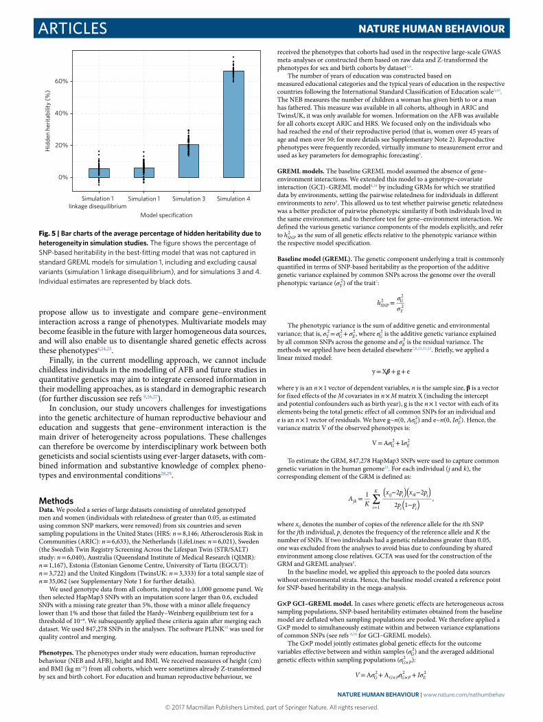
Fig. 5 | Bar charts of the average percentage of hidden heritability due to heterogeneity in simulation studies. The figure shows the percentage of SNP-based heritability in the best-fitting model that was not captured in standard GREML models for simulation 1, including and excluding causal variants (simulation 1 linkage disequilibrium), and for simulations 3 and 4. Individual estimates are represented by black dots.





where A is the GRM and AG×P is a matrix only with values for pairs of individuals within populations 1–7:

⎡

⎣

⎢⎢⎢⎢⎢⎢⎢⎢⎢⎢⎢⎢⎢⎢⎢⎢⎢⎢⎢

⎤

⎦

⎥⎥⎥⎥⎥⎥⎥⎥⎥⎥⎥⎥⎥⎥⎥⎥⎥⎥⎥

=A

A

A

A

A

A

A

A

A

A

A

A

A

A

A

A

A

A

A

A

A

A

A

A

A

A

A

A

A

A

A

A

A

A

A

A

A

A

A

A

A

A

A

A

A

A

A

A

A

A

p p

p p

p p

p p

p p

p p

p p

p p

p p

p p

p p

p p

p p

p p

p p

p p

p p

p p

p p

p p

p p

p p

p p

p p

p p

p p

p p

p p

p p

p p

p p

p p

p p

p p

p p

p p

p p

p p

p p

p p

p p

p p

p p

p p

p p

p p

p p

p p

p p

1 1

1 2

1 3

1 4

1 5

1 6

1 7

2 1

2 2

2 3

2 4

2 5

2 6

2 7

3 1

3 2

3 3

3 4

3 5

3 6

3 7

4 1

4 2

4 3

4 4

4 5

4 6

4 7

5 1

5 2

5 3

5 4

5 5

5 6

5 7

6 1

6 2

6 3

6 4

6 5

6 6

6 7

7 1

7 2

7 3

7 4

7 5

7 6

7 7

⎡

⎣

⎢⎢⎢⎢⎢⎢⎢⎢⎢⎢⎢⎢⎢⎢⎢⎢

⎤

⎦

⎥⎥⎥⎥⎥⎥⎥⎥⎥⎥⎥⎥⎥⎥⎥⎥

=×A

AA

AA

AA

A

000000

0

00000

00

0000

000

000

0000

00

00000

0

000000

G P

p p

p p

p p

p p

p p

p p

p p

1 1

2 2

3 3

4 4

5 5

6 6

7 7

The sums of both variance components (σ σ+ ×G G P2 2 ) were therefore expected

to correspond with the results of a meta-analysis of the sample-specific hSNP2 of

sufficient sample size. We quantified the hidden heritability due to heterogeneity as the discrepancy between = σ

σhSNP

2 GY

22 from the baseline model and = σ σ

σ+ ×hSNP

2 G G PY

2 22

from the G× P model.

G×C GCI–GREML model. We were likewise interested in gene–environment interaction across birth cohorts. Fertility behaviour and educational attainment have dramatically changed during the twentieth century16,34. Figure 1 shows the trends in AFB during the twentieth century for the countries in our study (see Supplementary Note 3 for details on the data sources). There is a well-established U-shaped pattern representing a falling AFB in the first half of the twentieth century followed by an upturn in the trend of AFB towards older ages. This widespread fertility postponement16—referred to as the second demographic transition35—was related to the spread of effective contraception, a drop in the NEB, changes in the economic need for children and female educational expansion16,36.

Environmental changes occurred at different periods in each country, with Australia having the earliest onset of fertility postponement (1939) and Estonia having the latest due to post-socialist transitions (1962) (see Supplementary Table 7 for all turning points and details). To test for gene–environment interaction, we grouped the birth cohorts into environmentally homogeneous conditions by those born before and those born after each country-specific fertility postponement turning point. To investigate the moderating effect of turning points, we followed the previous modelling strategy, but divided individuals into these turning point birth cohorts.

The G× C model is a joint model estimating the universal genetic effects for the traits effective between and within samples (σG

2) and the averaged additional genetic effects within defined birth cohorts (σ ×G C

2 ):

σ σ σ= + +× ×V A A IG G C G C E2 2 2

where A is the GRM and AG×C is a matrix only with values for pairs of individuals within the same demographic birth cohorts c1– c2:

⎡

⎣

⎢⎢⎢⎢⎢

⎤

⎦

⎥⎥⎥⎥⎥

=×AA 0

0 AG Cc c

c c

1 1

2 2

G×P×C GCI–GREML model. In the G× P× C model, we included both interaction terms mentioned above and an additional interaction term AG×P×C, which is equal to zero for all pairs of individuals living in different time periods or in different cohorts represented by:

σ σ σ σ σ= + + + +× × × × × × × ×V A A A A IG G P G P G C G C G P C G P C E2 2 2 2 2

where A is the GRM, AG×P is a matrix only with non-zero values for pairs of individuals within populations from the G× P model, AG×C is a matrix only with

non-zero values for pairs of individuals within the same demographic periods from the G× C model and AG×P×C is a matrix only with values for pairs of individuals with both the same demographic periods and the same populations.

Control variables. All phenotypes were Z-transformed by sampling population, birth year and sex. We also added fixed effects for sex, birth year, sampling population (with reference category LifeLines—the Dutch dataset) and the first 20 principal components calculated from the GRM across all populations to account for population stratification37. For the interaction model with birth cohorts, we included an additional fixed effect for the respective birth cohort turning point. In the G× P× C model, we additionally controlled for the interactions between the respective sampling population and the birth cohort division.

Model-fitting approach. The variance components were estimated using GREML estimation. When comparing the respective model specifications, to determine the best-fitting model, we relied on a model-fitting approach that compared the full model with reduced models that constrained specific effects to zero. Since the models were nested, we performed likelihood ratio tests and preferred the more parsimonious models if there was no significant loss in model fit (where the test statistic was distributed as a mixture of 0 and chi-squared (df = 1) with a probability of 0.5 (for details see ref. 8); P values from these tests are provided in Supplementary Tables 1–5). This strategy is also robust against the violation of the assumption of requiring a normal distribution of the dependent variable—as in the case of NEB, for example38.

Simulation study. We conducted a series of simulation studies to illustrate how our models interpret gene–environment interaction and to evaluate the role of potential alternative sources of heterogeneity in our data. All simulation studies are detailed in Supplementary Note 4 (for the theory behind them, see ref. 18). First, we were interested in how each model construed heterogeneity in heritability levels across populations. Since heritability is a ratio of the proportion of total phenotypic variance that is attributable to additive genetic effects, differences in the residual variance (for example, due to heterogeneous phenotypic measurement error) can lead to different levels of heritability across populations even though genetic effects are perfectly correlated. In contrast with twin studies, we were not interested in comparing levels of heritability across populations, but in the question of whether genes have the same effect on phenotypes across environments. We thus decomposed the heritability in the pooled data into additive genetic variance, both within and between environments.

In simple terms, we simulated phenotypes without gene–environment interaction across sampling populations and with gene–environment interaction across sampling populations based on 5,000 SNPs that were in approximate linkage equilibrium (pairwise r2 between SNPs below 0.05) and repeated this across 50 replications. First, to test for a model without gene–environment interaction, we set hSNP

2 of the trait to 0.50 and the genetic correlation across environments to 1 (Supplementary Note 4, simulation 1). Second, we repeated the simulations with varying residual phenotypic variance across populations39, resulting in simulated hSNP

2 to be between 0.25 and 0.625, but still with a genetic correlation of 1 across populations (Supplementary Note 4, simulation 2). Third, to illustrate weak levels of gene–environment interaction, we simulated hSNP

2 to be 0.50 and the genetic correlation of traits across populations to be 0.80 (Supplementary Note 4, simulation 3). Finally, to illustrate stronger gene–environment interaction, we simulated hSNP

2 to be 0.50 and the genetic correlation of traits across populations to 0.50 (Supplementary Note 4, simulation 4).

The stacked bars in Fig. 4 depict the average estimates of the four types of simulations for the simulated 50 phenotypes for the baseline model and the G× P model (individual estimates are presented as black dots for the full model and stripes in the bars represent variance components). Examining the first model (simulation 1) assumed no gene–environment interaction by sampling populations and thus homogeneous heritability. hSNP

2 as σ σ∕G Y2 2 (blue bar) is estimated at 0.324

and therefore around three-fifths of the simulated heritability of 0.50 since the GRM is based not only on quantitative trait loci. Central to our approach is that for the phenotypes with no G× P interaction, the variance explanation that is effective both within and between populations (σ σ∕G Y

2 2) is nearly identical to the baseline model (0.318). The gene–environment interaction term (σ σ∕×G P Y

2 2) estimates a small additional explanation of variance within populations of on average 0.026, with a full-model estimate of hSNP

2 within populations of 0.344 ⎛⎝⎜⎜

⎞⎠⎟⎟⎟=σ σ

σ+ ×G G P

Y

2 22 . Importantly, the same held when we simulated differences in hSNP

2 across populations due to varying residual variance. Simulation 2 in Fig. 4 shows an average hSNP

2 of 0.205 and G× P interaction model estimates of ‘universal’ genetic variance (σ σ∕G Y

2 2) of 0.200, with a gene–environment interaction term (σ σ∕×G P Y

2 2) of 0.0217. We therefore conclude that the model does not interpret heterogeneity in heritability levels due to differences in the residual variance as gene–environment interaction.

Simulations 3 and 4 in Fig. 4 depict how gene–environment interaction across sampling populations affects model estimates in scenarios of cross-population genetic correlations of 0.80 (weak) and 0.50 (strong) gene–environment interaction respectively, with the same population-specific hSNP

2 of 0.50 as in simulation 1.





First, we observed that hSNPs2 in the baseline models were deflated in the pooled

data ⎛⎝⎜⎜

⎞⎠⎟⎟⎟= . .σ

σ0 261 and 0 105G

Y

22 and therefore only captured around four-fifths and

one-third of the estimates in the absence of G× P, respectively. Second, when taking G× P into account, the full model estimate reached the same level as the baseline model in the absence of G× P ⎛

⎝⎜⎜

⎞⎠⎟⎟⎟= . .σ σ

σ+ × 0 328 and 0 315G G P

Y

2 22 due to a larger fraction

of genetic variance explained within populations ⎛⎝⎜⎜

⎞⎠⎟⎟⎟= . .σ

σ× 0 082 and 0 256G PY

22 and

did not appear to be inflated whatsoever. Third, the genetic variance explained effectively within and between populations in the G× P model was even smaller than in the baseline model ⎛

⎝⎜⎜

⎞⎠⎟⎟⎟= . .σ

σ0 246 and 0 059G

Y

22 . Therefore, while in the case of

a genetic correlation of 0.5 across populations within population estimates of hSNP2

capture around one-third of the overall heritability, the shared genetic variance explanation across populations would only be around 19% (0.059/0.315) of this value.

Based on the findings from simulation 4 for example, we would expect in the case of meta-analyses of population-specific GWAS on the gene–environment interaction phenotypes that genome-wide significant SNPs could explain only up to 10% of the variance while hSNP

2 of within populations could explain on average 32%. Around 68% of hSNP

2 (1–10/32) would therefore be ‘hidden’ in the mega-analysis due to heterogeneity and, in this case, due to gene–environment interaction.

Figure 5 shows hidden heritability estimates for the simulation without gene–environment interaction (simulation 1) and with gene–environment interaction (simulations 3 and 4). We were furthermore interested to find out to what extent genetic heterogeneity across populations such as differences in genetic measurement, linkage disequilibrium across sampling populations or heterogeneous imputation quality across populations could lead to observed heterogeneity or deflate hSNP

2 in pooled data sources. To investigate this, we removed the 5,000 causal SNPs from the genetic data, which was the basis of how we simulated the phenotypes. We then re-estimated the GRM and repeated the analyses on simulation 1 of phenotypes without gene–environment interaction and homogeneous heritability across populations (depicted in Fig. 5 as simulation 1 linkage disequilibrium). When the causal SNPs were removed, estimates were based on correlated SNPs which were in linkage disequilibrium. To the extent that the structure in the genetic data we used was heterogeneous across populations, we would expect our models to interpret this heterogeneity as heterogeneous genetic effects resulting in hidden heritability.

Figure 5 shows that hidden heritability was estimated to be around 68% for a genetic correlation of 0.50, around 20% for a genetic correlation of 0.80 and around 5% for the model without gene–environment interaction as well as a model based on SNPs in linkage disequilibrium with the causal SNPs. This allowed us to draw two conclusions. First, in the complete absence of gene–environment interaction (simulation 1), our models interpreted (on average, across 50 simulations) that 5% of the heritability in the G× P model was hidden in a standard model, with a statistically significant G× P term in 10 simulation studies (20%; not listed) at the 5% level. It was important to keep this in mind when analysing phenotypes of interest. To evaluate phenotype-specific model inflations, we conducted complementary permutation analyses generating a matrix with randomly stratified environments to see how estimates were inflated in the real data for specific phenotypes. Second, we found no difference in inflation between the simulations including and excluding causal SNPs (simulation 1 linkage disequilibrium and simulation 1). We conclude from this that heterogeneity in the genetic structure of the populations did not affect our interpretation of gene–environment interaction in comparison with the standard model. This is probably due to the fact that we only looked at common SNPs and applied rigorous quality control. To investigate whether gene–environment interaction was present for education and human reproductive behaviour, we applied the above models as well as G× C and G× P× C models to these phenotypes in seven sampling populations.

Sex differences. Previous whole-genome studies found no evidence for gene–sex interaction of common genetic effects on BMI, height19 and also human reproductive behaviour6 (note that a family-based study showed evidence for sexual dimorphism in childlessness40). We also tested for gene–sex interaction within sampling populations in our data, as:

σ σ σ= + +× × × × × ×V A A IG P G P G P sex G P sex E2 2 2

where AG×P is the GRM only with values for pairs of individuals within the same population and AG×P×sex is a matrix with only values for pairs of individuals of the same sex and same sampling population.

Decomposing the genetic variance of all five phenotypes (height, BMI, education, NEB and AFB) into within-population effects shared between sexes (σ ×G P

2 ) and the averaged additional genetic effects within sexes (σ × ×G P sex2 ), we found

no evidence for sex-specific effects (σ × ×G P sex2 ) for education (P = 0.49), AFB

(P = 0.5), NEB (P = 0.41) or height (P = 0.5). Only for BMI did we find evidence

of a roughly 3% sex-specific variance explanation (P = 0.046; for full results see Supplementary Table 8). Given that we focused on education and reproductive behaviour, we applied all models to pooled data including both sexes, keeping in mind the findings for BMI.

Data availability. The Database of Genotypes and Phenotypes (dbGaP) data that support the findings of this study are publicly available from the ARIC study (dbGaP phs000090.v1.p1) and the HRS (dbGaP phs000428.v1.p1). Access to individual-level phenotypic and genetic data from the QIMR, the EGCUT, the STR/SALT study, TwinsUK and the LifeLines study will be available once a research agreement has been obtained (see Supplementary Note 1).

Received: 26 January 2017; Accepted: 4 August 2017; Published: xx xx xxxx

References 1. Visscher, P. M. et al. 10 years of GWAS discovery: biology, function, and

translation. Am. J. Hun. Genet. 101, 5–22 (2017). 2. Manolio, T. A. et al. Finding the missing heritability of complex diseases.

Nature 461, 747–753 (2009). 3. Witte, J. S., Visscher, P. M. & Wray, N. R. The contribution of genetic variants

to disease depends on the ruler. Nat. Rev. Genet. 15, 765–776 (2014). 4. Polderman, T. J. C. et al. Meta-analysis of the heritability of human traits

based on fifty years of twin studies. Nat. Genet. 47, 702–709 (2015). 5. Okbay, A. et al. Genome-wide association study identifies 74 loci associated

with educational attainment. Nature 533, 539–542 (2016). 6. Barban, N. et al. Genome-wide analysis identifies 12 loci influencing human

reproductive behavior. Nat. Genet. 48, 1462–1472 (2016). 7. Yang, J. et al. Common SNPs explain a large proportion of the heritability for

human height. Nat. Genet. 42, 565–569 (2010). 8. Yang, J., Lee, S. H., Goddard, M. E. & Visscher, P. M. GCTA: a tool for

genome-wide complex trait analysis. Am. J. Hum. Genet. 88, 76–82 (2011).

9. Tropf, F. C. et al. Human fertility, molecular genetics, and natural selection in modern societies. PLoS ONE 10, e0126821 (2015).

10. Rietveld, C. A. et al. GWAS of 126,559 individuals identifies genetic variants associated with educational attainment. Science 340, 1467–1471 (2013).

11. Zhu, Z. et al. Dominance genetic variation contributes little to the missing heritability for human complex traits. Am. J. Hum. Genet. 96, 377–385 (2015).

12. Zuk, O. & Hechter, E. The mystery of missing heritability: genetic interactions create phantom heritability. Proc. Natl Acad. Sci. USA 109, 1193–1198 (2012).

13. Yang, J. et al. Genetic variance estimation with imputed variants finds negligible missing heritability for human height and body mass index. Nat. Genet. 47, 1114–1120 (2015).

14. Felson, J. What can we learn from twin studies? A comprehensive evaluation of the equal environments assumption. Soc. Sci. Res. 43, 184–199 (2014).

15. Wray, N. R. et al. Pitfalls of predicting complex traits from SNPs. Nat. Rev. Genet. 14, 507–515 (2013).

16. Mills, M. C., Rindfuss, R. R., McDonald, P. & te Velde, E. Why do people postpone parenthood? Reasons and social policy incentives. Hum. Reprod. Update 17, 848–860 (2011).

17. De Vlaming, R. et al. Meta-GWAS Accuracy and Power (MetaGAP) calculator shows that hiding heritability is partially due to imperfect genetic correlations across studies. PLOS Genet. 13, e1006495 (2017).

18. Robinson, M. R. et al. Genotype-covariate interaction effects and the heritability of adult body mass index. Nat. Genet. 49, 1174–1181 (2017).

19. Yang, J. et al. Genome-wide genetic homogeneity between sexes and populations for human height and body mass index. Hum. Mol. Genet. 24, 7445–7449 (2015).

20. Conley, D., Laidley, T. M., Boardman, J. D., Domingue, B. W. & Boardman, J. D. Changing polygenic penetrance on phenotypes in the 20th century among adults in the US population. Sci. Rep. 6, 30348 (2016).

21. Walter, S. et al. Association of a genetic risk score with body mass index across different birth cohorts. JAMA 316, 63–69 (2016).

22. Mehta, D. et al. Evidence for genetic overlap between schizophrenia and age at first birth in women. JAMA Psychiatry 73, 497–505 (2016).

23. Visscher, P. M. et al. Statistical power to detect genetic (co) variance of complex traits using SNP data in unrelated samples. PLoS Genet. 10, e1004269 (2014).

24. Briley, D. A., Tropf, F. C. & Mills, M. C. What explains the heritability of completed fertility? Evidence from two large twin studies. Behav. Genet. 47, 36–51 (2017).

25. Tropf, F. C. & Mandemakers, J. J. Is the association between education and fertility postponement causal? The role of family background factors. Demography 54, 71–91 (2017).

26. Mills, M. C. Introducing Survival and Event History Analysis (Sage, Thousand Oaks, CA, 2011).





27. Tropf, F. C., Barban, N., Mills, M. C., Snieder, H. & Mandemakers, J. J. Genetic influence on age at first birth of female twins born in the UK, 1919–68. Popul. Stud. (Camb.) 69, 129–145 (2015).

28. Stearns, S. C., Byars, S. G., Govindaraju, D. R. & Ewbank, D. Measuring selection in contemporary human populations. Nat. Rev. Genet. 11, 611–622 (2010).

29. Courtiol, A., Tropf, F. C. & Mills, M. C. When genes and environment disagree: making sense of trends in recent human evolution. Proc. Natl Acad. Sci. USA 113, 7693–7695 (2016).

30. Purcell, S. M. et al. PLINK: a tool set for whole-genome association and population-based linkage analyses. Am. J. Hum. Genet. 81, 559–575 (2007).

31. Lee, S. H., Yang, J., Goddard, M. E., Visscher, P. M. & Wray, N. R. Estimation of pleiotropy between complex diseases using single-nucleotide polymorphism-derived genomic relationships and restricted maximum likelihood. Bioinformatics 28, 2540–2542 (2012).

32. Visscher, P. M., Yang, J. & Goddard, M. E. A commentary on ‘common SNPs explain a large proportion of the heritability for human height’ by Yang et al. (2010). Twin Res. Hum. Genet. 13, 517–524 (2010).

33. International HapMap 3 Consortium. Integrating common and rare genetic variation in diverse human populations. Nature 467, 52–58 (2010).

34. Balbo, N., Billari, F. C. & Mills, M. C. Fertility in advanced societies: a review of research. Eur. J. Popul. 29, 1–38 (2013).

35. Van de Kaa, D. J. Europe’s second demographic transition. Popul. Bull. 42, 1–59 (1987).

36. Sobotka, T. Is lowest‐low fertility in europe explained by the postponement of childbearing? Popul. Dev. Rev. 30, 195–220 (2004).

37. Price, A. L. et al. Principal components analysis corrects for stratification in genome-wide association studies. Nat. Genet. 38, 904–909 (2006).

38. Snijders, T. A. B. Multilevel Analysis (Springer, Berlin, 2011). 39. Domingue, B. W. et al. Genome-wide estimates of heritability for social

demographic outcomes. Biodemography Soc. Biol. 62, 1–18 (2016). 40. Verweij, R. M. et al. Sexual dimorphism in the genetic influence on human

childlessness. Eur. J. Hum. Genet. 25, 1067–1074 (2017). 41. Mills, M. C. & Tropf, F. C. The biodemography of fertility: a review and

future research frontiers. Kolner Z. Soz. Sozpsychol. 55, 397–424 (2016). 42. Visscher, P. M., Hill, W. G. & Wray, N. R. Heritability in the genomics

era—concepts and misconceptions. Nat. Rev. Genet. 9, 255–266 (2008). 43. Wray, N. R. & Maier, R. Genetic basis of complex genetic disease: the

contribution of disease heterogeneity to missing heritability. Curr. Epidemiol. Rep. 1, 220–227 (2014).

AcknowledgementsFunding was provided by the European Research Council Consolidator Grant SOCIOGENOME (615603) and the UK Economic and Social Research Council/National Centre for Research Methods SOCGEN grant (ES/N011856/1), as well as the Wellcome Trust Institutional Strategic Support Fund and John Fell Fund (awarded to M.C.M.). The ARIC study is carried out as a collaborative study supported by the United States National Heart, Lung, and Blood Institute (HHSN268201100005C, HHSN268201100006C, HHSN268201100007C, HHSN268201100008C, HHSN268201100009C, HHSN268201100010C, HHSN268201100011C and HHSN268201100012C). The EGCUT study was supported by European Union Horizon 2020 grants 692145, 676550 and 654248, Estonian Research Council Grant IUT20-60, the Nordic Information for Action e-Science Center, the European Institute of Innovation and Technology–Health, National Institutes of Health (NIH) BMI grant 2R01DK075787-06A1 and the European Regional Development Fund (project 2014-2020.4.01.15-0012 GENTRANSMED). The Health and Retirement Study is supported by the United States

National Institute on Aging (U01AG009740). The genotyping was funded separately by the United States National Institute on Aging (RC2 AG036495 and RC4 AG039029) and was conducted by the NIH Center for Inherited Disease Research (CIDR) at Johns Hopkins University. Genotyping quality control and final preparation of the HRS data were performed by the Genetics Coordinating Center at the University of Washington. The LifeLines Cohort Study and generation and management of GWAS genotype data for the LifeLines Cohort Study were supported by the Netherlands Organisation for Scientific Research (NWO 175.010.2007.006), Economic Structure Enhancing Fund of the Dutch government, Ministry of Economic Affairs, Ministry of Education, Culture and Science, Ministry for Health, Welfare and Sports, Northern Netherlands Collaboration of Provinces, Province of Groningen, University Medical Center Groningen, University of Groningen, Dutch Kidney Foundation and Dutch Diabetes Research Foundation. The Swedish Twin Registry (TWINGENE) was supported by the Swedish Research Council (M-2005-1112), GenomEUtwin (EU/QLRT-2001-01254 and QLG2-CT-2002-01254), NIH DK U01-066134, Swedish Foundation for Strategic Research and Heart and Lung Foundation (20070481). The TwinsUK study was funded by the Wellcome Trust and European Community’s Seventh Framework Programme (FP7/2007–2013). The study also received support from the National Institute for Health Research-funded BioResource, Clinical Research Facility and Biomedical Research Centre based at Guy’s and St Thomas’ NHS Foundation Trust in partnership with King’s College London. SNP genotyping was performed by The Wellcome Trust Sanger Institute and National Eye Institute via the NIH CIDR. For the QIMR data, funding was provided by the Australian National Health and Medical Research Council (241944, 339462, 389927, 389875, 389891, 389892, 389938, 442915, 442981, 496739, 552485 and 552498), Australian Research Council (A7960034, A79906588, A79801419, DP0770096, DP0212016 and DP0343921), FP-5 GenomEUtwin Project (QLG2-CT-2002-01254) and NIH (grants AA07535, AA10248, AA13320, AA13321, AA13326, AA14041, DA12854 and MH66206). A portion of the genotyping on which the QIMR study was based (the Illumina 370 K scans) was carried out at the CIDR through an access award to the authors’ late colleague R. Todd (Psychiatry, Washington University School of Medicine, St Louis). Imputation was carried out on the Genetic Cluster Computer, which is financially supported by the Netherlands Organisation for Scientific Research (NWO 480-05-003). The funders had no role in study design, data collection and analysis, decision to publish or preparation of the manuscript.

Author contributionsF.C.T., S.H.L. and M.C.M. developed the study concept and design. M.R.R. and F.C.T. developed the concept for and performed the simulation studies. F.C.T., R.M.V., G.S. and C.R. performed the data analysis and visualization. T.E., A.M., S.E.M., N.G.M., A.N., S.H.L. and A.B. provided data and input on data analysis and interpretation, and imputed the data. F.C.T., M.C.M., S.H.L., M.R.R., H.S., G.S. and R.d.V. drafted the manuscript. F.C.T., M.C.M., M.R.R., R.M.V., G.S., P.J.v.d.M., R.d.V., N.G.M., N.B., D.A.B., C.R. and R.H. revised the manuscript. All authors approved the final version of the manuscript for submission.

Competing interestsThe authors declare no competing interests.

Additional informationSupplementary information is available for this paper at doi:10.1038/s41562-017-0195-1.Reprints and permissions information is available at www.nature.com/reprints.Correspondence and requests for materials should be addressed to F.C.T.Publisher’s note: Springer Nature remains neutral with regard to jurisdictional claims in published maps and institutional affiliations.


http://dx.doi.org/10.1038/s41562-017-0195-1

http://dx.doi.org/10.1038/s41562-017-0195-1

http://www.nature.com/reprints


hidden heritability due to heterogeneity across seven

Documents