hidden markov models pavel chigansky
TRANSCRIPT

Hidden Markov Models
Pavel Chigansky
Department of Statistics, The Hebrew University, Mount Scopus, Jerusalem91905, Israel
E-mail address: [email protected]

Key words and phrases. probability, stochastic processes, statistics, estimation, Markovprocesses

3
Preface
These are the lecture notes for the graduate course I taught at the Statistics De-partment of the Hebrew University. The main focus is on theoretical aspects of HMMs(the reader already familiar with mathematical probability is advised to skip Chapter2). Please do not hesitate to send your comments/bug reports, etc. to the [email protected]
P.Ch., February 26, 2012


Contents
Chapter 1. A short prelude 7
Chapter 2. Preliminaries 111. Probability theory: a vocabulary 112. Elements of Markov processes 293. Hidden Markov Models 35
Chapter 3. Hidden state estimation 411. Filtering, Prediction and Smoothing 422. Finite dimensional filters 523. Approximations 694. Filter stability 79
Chapter 4. Inference 851. Generalities 852. The EM algorithm 86
Bibliography 93
5


CHAPTER 1
A short prelude
Suppose we have a capital of x dollars, which we would like to invest to make a profit.One possibility is to put the money in a bank and enjoy a constant interest rate r > 0,so that in n time units the initial sum grows to x(1 + r)n. Another possibility is to buya stock and to sell it at some point in the future. This is a risky investment, as it doesnot guarantee certain profit, but may yield an effective interest rate, higher than r withconsiderable probability. A simple way to model the stock prices S = (Sn)n≥0 is to assumethat they grow at a random rate, i.e.
Sn = Sn−1(1 + εn), n ≥ 1, (1a1)
subject to S0 = 1, where ε = (εn)n≥1 are i.i.d. random variables with values in (−1,∞).So if we invest the whole sum in the stock, we will obtain x
∏nm=1(1 + εm) dollars after
n time units. Notice that by the independence of εn’s, the conditional distribution of Sn,given the history of prices S1, ..., Sm, m < n depends only on the latest price Sm, i.e.P (Sn ≤ y|S1, ..., Sm) = P (Sn ≤ y|Sm), y ∈ R. This is the Markov property (Sn’s are saidto form a Markov chain), which will play a major role in this course.
The next obvious goal is to calibrate the model, i.e. to estimate the probabilitydistribution of ε1. For example, one can assume that ε1 is distributed uniformly on aninterval [a, b] with b > a > −1 and to use one of the standard statistical techniques toestimate a and b, given the data S1, ..., Sn. In particular, the following estimates
an = min(S1, S2/S1, ..., Sn/Sn−1
)− 1
bn = max(S1, S2/S1, ..., Sn/Sn−1
)− 1(1a2)
enjoy various nice properties, including consistency, i.e. an → a and bn → b as n → ∞,which means that we can estimate a and b with any desired precision if enough data isavailable.
Our ultimate goal is to make as much money as possible at a given time N > 0. Theobvious strategy is to divide the sum accumulated up to time n into two parts, one ofwhich is put into the bank account and one is used to buy the stock (to be sold at timen + 1). If Xn denotes the amount of money at our disposal at the end of n-th time unitand un ∈ [0, 1] stands for the proportion of Xn we leave at the bank for the next timeepoch, the total amount of money we obtain at time n+ 1 is given by
Xn+1 = Xnun(1 + r) +Xn(1− un)(1 + εn+1), n ≥ 0. (1a3)
The problem is then to choose the strategy u = (un)n∈[0,N−1] to maximize the expectedvalue ofXN or, more generally, of F (XN ) for a nonnegative utility function F (for example,F (x) = log x). The choice of un must depend only on the information available up to time
7

8 1. A SHORT PRELUDE
n, i.e. on the stock prices observed up to the current moment or equivalently on ε1, ..., εn.This a classical problem of optimal control and it can be solved using the dynamicalprogramming method, to be encountered in this course on several occasions.
The i.i.d. assumption of the model (1a1) can be reasonable on short time periods,when nothing drastic happens to economy, politics, company health, etc. Such changesmay or may not be disclosed to the public, but once they occur, the market is likely toreact by changing its parameters.
To incorporate such phenomena into the model, one can assume that the marketoperates in one of several distinct regimes, which are switched at random time to time,depending on the global economical climate. More precisely, let (Zn)n≥0 be a Markovchain with values in 1, ..., d, transition probabilities λij = P (Zn = j|Zn−1 = i) andinitial distribution ν(i) = P (Z0 = i), i = 1, ..., d. Let εn be an i.i.d. sequence of randomvectors, whose entries have different probability densities (naturally ψi(y) = 0 for y < −1)
P(εn(i) ≤ y
)=
∫ y
−∞ψi(r)dr, i = 1, ..., d.
Assume that ε and Z are independent and define
Sn = Sn−1
(1 + εn(Zn)
), n ≥ 1. (1a4)
The latter means that the stock follows the dynamics of the form (1a1), whose parametersare switched by Zn.
The state or the signal Z is hidden in the sense that it cannot be directly accessed andall the statistical information about it is to be inferred from observations of the stock priceprocess S alone. The pair (Z, S), which is a Markov process as well, is a typical exampleof a Hidden Markov Model (also known as state space models, partially observed systems,etc.).
As we will see, one of the key ingredients of various statistical questions related toHMM is the filtering conditional distribution
πn(i) = P(Zn = i|S1, ..., Sn), i = 1, ..., d.
In particular, having seen the prices up to time n, we will minimize the expected error ofguessing the current state of Zn, if we choose the state i maximizing πn(i):
P(argmax
iπn(i) 6= Zn
) ≤ P(ζn 6= Zn),
for any random variable of the form ζn = Fn(S1, ..., Sn) with Fn : Rn 7→ 1, ..., d.Due to the Markov structure of the model, the process πn satisfies the (vector) recur-
sion:
πn =Ψ(Sn/Sn−1 − 1
)Λ∗πn−1∥∥Ψ(Sn/Sn−1 − 1)Λ∗πn−1
∥∥ , π0 = ν (1a5)
where ‖ · ‖ stands for the `1-norm (sum of absolute values), Λ∗ is transposed of thetransition probabilities matrix and Ψ(y) is a diagonal matrix with Ψii(y) = ψi(y). Thealgorithm (1a5) generates πn on-line, i.e. the new value of πn is recalculated on the basisof its previous value and the newly observed price. We don’t have to store all the pricesbackwards to calculate πn, as all the relevant information is kept in πn−1, which can be

1. A SHORT PRELUDE 9
a significant practical advantage. The recursion (1a5) is called the filtering equation orsimply the filter.
Calculation of πn requires knowledge of all the parameters, namely the size of thealphabet d, the initial distribution ν of the hidden state, the transition probabilities λij
and the emitting densities ψi(y). It turns out that parameter estimation for HMM isessentially harder than e.g. for the model (1a1). For example, the estimates of the type(1a2) cannot be applied anymore, as the current regime of the market is not observed.Recalling that (1a2) emerge as maximizers of the likelihood function, corresponding to(1a1), one can find estimates for the HMM parameters by maximizing the appropriatelikelihood function. Such optimization unfortunately does not yield a closed form solutionin general and thus is to be carried out numerically. The performance analysis of theseestimates often poses mathematical challenges.
Once the inference is done and the model is fitted, we can return to the profits opti-mization problem. This time our money satisfies the recursion
Xn+1 = Xnun(1 + r) +Xn(1− un)(1 + εn(Zn)
)
and our goal is to choose un ∈ [0, 1], n = 1, ..., N , to maximize EXN at some fixed time N .This control problem is essentially more complicated than the one associated with (1a3), asthe random variables εn(Zn) are not i.i.d. and not even Markov. Still the optimal strategycan be characterized, by reformulating the problem in terms of the filtering process πn.
Beside of being a useful modeling paradigm, HMMs pose interesting and challengingmathematical questions, which do not cease to generate exciting research. This coursefocuses on the latter and almost completely ignores the former. We shall define and treatHMM abstractly, aiming to exhibit the rigorous part of the story (similarly to the texts[13], [7], see also the survey [14]).


CHAPTER 2
Preliminaries
1. Probability theory: a vocabulary
“Probability theory is measure theory with a soul”, M. Kac
The goal of this section is to refresh the basic concepts of measure theoretic probability.We shall only touch upon the necessary minimum to be able to get started with the maintheme of this course and will cover more as the story unfolds. Further exploration is verymuch encouraged: e.g. [41] is an excellent solid introduction into the subject.
1.1. n independent tosses of a fair coin. The canonical example of probabilitytheory is n independent tosses of a fair coin. Typically we would like to be able
(Q1) to calculate the probabilities of various events, related to such an experiment fora fixed n ≥ 1: for example, to find the probability that there are more heads inn tosses than tails.
(Q2) to study the behavior of these events as n → ∞: for example, to find the limitof the probability that the proportion of heads deviate from 1/2 by more than afixed small number ε > 0.
To find the answers to this kind of questions, a mathematical model is required. Let’sparse the phrase carefully: “n [...] tosses of a [...] coin” means that we have an experiment,which yields one of the 2n possible outcomes, namely a string of heads and tails (labeledH and T ) of length n. In the language of probability theory we have a sample space Ω,which consists of 2n points ω ∈ Ω or elementary events, each being a word of length n,composed of letters H and T . We shall index the words by a superscript and the symbolsin each word by a subscript, that is we enumerate the points in Ω = ω1, ..., ω2n, so thate.g. ωm
j means the outcome of the j-th toss in the m-th word.We are of course interested to consider events, other than just elementary ones: for
example, as in (Q1) above, or the event of getting an even number of heads (denote it byA), or the event of getting tails in the last and the first tosses (denoted it by B), etc. Eachsuch event is a subset of Ω. For example,
A =
ω ∈ Ω :
n∑
i=1
1ωi=H = 2k for some k = 0, ..., 2n−1
(2a1)
and
B = ω ∈ Ω : ω1 = T, ωn = T . (2a2)
Being a subset of (our finite) Ω, any event is of course a union of a number of elementaryevents and the event occurs if any of these elementary events occurs. How many eventsare there ? In the finite case |Ω| < ∞, any subset of Ω can be considered as an event and
11

12 2. PRELIMINARIES
the power set can be taken as the space of all events, which means that this experimentproduces 22
nevents (including the empty set ∅). Of course, one can define a smaller
collection of events (see Exercise 2 below). We shall denote the space (collection) ofevents by F and in this case the natural choice is F := 2Ω (the power set, i.e. the set of alsubsets of Ω).
Exercise 1. List all the events in F = 2Ω for n = 2.
Further, notice that A1 ∩ A2 occurs if an ω ∈ A1 ∩ A2 occurs, i.e. an ω from bothA1 and A2 occurs or both A1 and A2 occur. Hence intersection of sets means that thecorresponding events occur simultaneously. Similarly union of sets means that at leastone of the corresponding events occurs. Naturally we would like to be able to includeintersections and/or unions and/or compliments of events as events on their own or inother words, our collection of events F is to be closed under taking unions, intersectionsand compliments: if A1, A2 ∈ F then A1 ∩ A2 ∈ F and A1 ∪ A2 ∈ F and Ac
1 ∈ F. Such acollection of sets is called algebra of sets (events). Clearly F := 2Ω is an algebra.
Exercise 2. Show that G := ∅, A,Ac,Ω is an algebra of events for any event A ⊆ Ω.
What does “fair” and ”independent” mean ? This has to do with the probabilityfunction yet to be assigned to each event from F. Thus probability is a set function Pdefined on F, taking values in the interval [0, 1]. If A and B are mutually exclusive, i.e.cannot happen simultaneously, it is natural to require that probability of their union, i.e.that either A or B happens, equals to the sum of their probabilities:
A ∩B = ∅ =⇒ P(A ∪B) = P(A) + P(B). (2a3)
Exercise 3. Show that (2a3) implies
P(A ∪B) = P(A) + P(B)− P(A ∩B),
and
P(Ω) = 1, (2a4)
and for any m ≥ 1
P(∪mi=1Ai) =
m∑
i=1
P(Ai).
where Ai ∈ F are pairwise disjoint events.
By saying that a coin is fair, we mean that our expectancy of either heads or tails ineach single toss is the same. In terms of the structure introduced so far this implies
P(ω : ωi = H) = P(ω : ωi = T ), ∀i = 1, ..., n.
Since ω : ωi = H ∪ ω : ωi = T = Ω and P(Ω) = 1, the latter is equivalent to
P(ω : ωi = H) = 1/2, ∀i = 1, ..., n. (2a5)
Independence of tosses is expressed by requiring that
P(ω : ωi1 = x1, ..., ωik = xk) = P(ω : ωi1 = x1)...P(ω : ωik = xk) (2a6)
is satisfied for any xi ∈ H,T, i1, ..., ik ∈ 1, ..., n and integer k ≤ n.

1. PROBABILITY THEORY: A VOCABULARY 13
Exercise 4. The conditional probability of a set A, given set B with P(B) > 0 oc-curred, is defined as P(A|B) := P(A ∩B)/P(B). Explain (2a6) in view of this definition.
Exercise 5. Show that the only P : F 7→ [0, 1], satisfying (2a3)-(2a6), takes equalvalues on the elementary events:
P(ω) =1
|Ω| = 2−n, ∀ω ∈ Ω. (2a7)
Since any set A ∈ F is a finite union of elementary events, P is defined for any A ∈ F
once it is defined for any ω ∈ Ω by (2a3):
P(A) =∑
ωi∈AP(ωi).
To summarize, we have explicitly
(1) defined the sample space Ω as a collection of points or elementary events(2) chosen the algebra of events F(3) assigned the additive (i.e. satisfying (2a3)) probability function P : F 7→ [0, 1].
Thus we have introduced the probability space (Ω,F,P), which allows to calculate proba-bilities of any events under consideration (i.e. those included in F).
Exercise 6. Calculate the probability of the event, mentioned in Q1
Exercise 7. Calculate the probabilities of the events A from (2a1) and B from (2a2).
Exercise 8. Show that the probability of the event, mentioned in Q2, tends to zero asn → ∞, i.e. verify the weak law of large numbers for Bernoulli i.i.d. sequence:
limn→∞Pn
(ω ∈ Ωn :
∣∣∣ 1n
n∑
m=1
1ωi=1 −1
2
∣∣∣ ≥ ε
)= 0, ∀ε > 0,
where (Ωn,Fn,Pn) is the probability space corresponding to n tosses. Hint: prove anduse the Chebyshev inequality: for any nonnegative real function (a.k.a. random variable)X : Ω 7→ R over a probability space (Ω,F,P)
P(X ≥ a) ≤ EX2
a2.
1.2. Infinitely many independent tosses of a fair coin. Consider now the ex-periment of infinitely many independent tosses of a fair coin. We are after a mathematicalmodel, which would still be useful to answer questions like (Q1) and (Q2) (after all ntosses can be always extracted from infinitely many ones!), but we also would like to beable
(Q3) to calculate probabilities of the events, depending on infinitely many tosses: forexample, to find probability of the event that the proportion of heads in all thetosses is exactly 1/2 (the strong law of large numbers)
Let’s try to mimic the structure introduced in the previous section. The outcome of ourinfinite experiment is an infinite sequence of symbols H and T , i.e. an elementary eventω is
ω = ω1, ω2, ..., ωi ∈ H,T, ∀i ≥ 1.

14 2. PRELIMINARIES
How many ω’s are there in Ω = H,T∞ ? Note that if we identify H with 1 and T with0, we can view each ω as a binary expansion of a number in the interval [0, 1]. There arepairs of sequences which correspond to the same number, namely those whose digits areall ones started from certain index. For example, 010000... and 001111... both representthe same number 1/4. However all such pairs can represent only rational numbers, i.e. wehave at most countable number of such “collisions”. In what follows, it will become clearthat all of them will be assigned negligible probability and hence can be excluded from Ωe.g. in consideration of questions as (Q1)-(Q3).
So after removing all the sequences which end with infinite number of 1’s, we have aone-to-one correspondence between the rest of the sequences in our experiment and thepoints in [0, 1]. Hence roughly, our experiment generates at least as many elementaryevents as there are points in [0, 1], i.e. Ω contains uncountably many points.
Which subsets of Ω should we consider as events, i.e. how should we define F ?Definitely we should include the cylindrical sets, i.e. the events of the form:
ω ∈ Ω : ωi1 = x1, ..., ωim = xm , m ∈ Z+, i1, ..., im ∈ Z+, xi ∈ 0, 1,as they can be naturally associated with the finite number of tosses.
Exercise 9. Show that a cylindrical set in Ω = 0, 1∞ correspond to a union ofintervals with dyadic endpoints.
Next, we would still like our F to be an algebra, i.e. to be closed under finite numberof intersections and/or unions. Notice that in this case the algebra of all cylindrical setsis countably infinite (unlike in the case of n tosses).
Exercise 10. Show that the collection of all cylindrical sets is an algebra.
Certainly we would like to consider events such as the one from (Q3):
C =
ω ∈ Ω : lim
n→∞1
n
n∑
k=1
1ωk=1 = 1/2
. (2a8)
Is it in the algebra we have defined so far ? In other words, can it be obtained from afinite number of cylindrical sets by means of unions and/or intersections ?
Exercise 11. Argue that the answer is negative.
However
C = ∩k≥1 ∪m≥1 ∩n≥mAn,k (2a9)
where An,k =
ω ∈ Ω :
∣∣∣ 1n∑n
m=1 1ωm=1 − 1/2∣∣∣ ≤ 1/k
, are cylindrical (and hence
already accepted by us as events). Thus it is natural to require that F be closed undercountably infinite number of unions/intersections, that is to require F to be a σ-algebra.If we do so, automatically events obtained by the limit procedure as in (2a9) are captured.
Exercise 12. Let An, n ≥ 1 be a sequence of sets. Argue that the following sets
limn→∞An := ∩n≥1 ∪m≥n Am, lim
n→∞An := ∪n≥1 ∩m≥n Am.

1. PROBABILITY THEORY: A VOCABULARY 15
are well defined1. Explain why Ai.o. := limn→∞An consists of all the points encounteredin the sequence An infinitely often and Ae := limn→∞An consists of the points eventuallyencountered in all the entries of the sequence An.
Thus F = σA, the σ-algebra generated by the algebra A of cylindrical sets, i.e. thesmallest σ-algebra, containing A, is one of our candidates.
Exercise 13. Why the smallest σ-algebra always exists ? Hint: exhibit at least oneσ-algebra which contains A and use the fact that an intersection of σ-algebras is a σ-algebra.
The σ-algebra is a much richer collection of sets than the generating algebra.
Exercise 14. Show that the following events belong to the σ-algebra F = σA (orequivalently are measurable with respect to F)
H is encountered infinitely often
the sequence of tosses is periodic
the sequence of tosses terminates with an infinite sequence of H’s
What properties should we expect our probability function P satisfy ? Certainly, wewould still want P(Ω) = 1, P(A) ≥ 0 and additivity of P. However, since we want toinclude infinite unions/intersections into F, we shall require P to be countably additive orσ-additive, i.e.
An ∈ F, Ai ∩Aj = ∅ ∀i 6= j =⇒ P(∪∞n=1 An
)=
∞∑
n=1
P(An). (2a10)
Exercise 15. Show that σ-additivity P is equivalent to continuity of P, which meansthat for any sequence of events An, such that limn→∞An is well defined2
P( limn→∞An) = lim
n→∞P(An).
Hint: first, argue that no generality is lost if we show that P is continuous at zero, i.e. An
monotonously decreases to ∅. Show that in the latter case, limn→∞An = ∩n≥0An equalsa union of some sequence of pairwise disjoint events.
The structure we have obtained so far is precisely the set of axioms of probabilitytheory due to A.Kolmogorov (1933): the probability space (Ω,F,P) consists of
(a) the sample space Ω, i.e. a set of points (elementary events) ω ∈ Ω(b) a σ-algebra F of subsets (events) of Ω, i.e. a collection of subsets satisfying
Ω ∈ F
A ∈ F =⇒ Ac ∈ F
An ∈ F =⇒ ∩∞n=1An ∈ F
An ∈ F =⇒ ∪∞n=1An ∈ F
(c) a σ-additive function (measure) P : F 7→ [0, 1] (probability)
1Compare to the definition of the corresponding limits of numbers2i.e. limn→∞ An = limn→∞ An =: limn→∞ An

16 2. PRELIMINARIES
At this point one may wonder why not to choose F to be the power set of Ω as in thefinite experiment: after all it is a σ-algebra in particular. The reason is that one cannotconstruct a reasonably useful probability measure on such a “big” σ-algebra: for example,there is no probability measure on the power set of [0, 1], which assigns intervals theirlengths. This raises the question of how probability measures can be constructed ? Themain tool is the following theorem:
Theorem 1.1 (C.Caratheodory). Let Ω be a set, A be an algebra of its subsets andσA be the minimal σ-algebra containing A. Let µ0 be a finite3 countably additive mea-sure on (Ω,A). Then there is a unique measure µ on (Ω, σA), whose restriction on A
coincides with µ0, i.e. µ(A) = µ0(A) whenever A ∈ A.
Here is what this Theorem tells us in the context of infinitely many coin tosses. Let Abe the algebra of cylindrical sets of 0, 1∞ and let B be the σ-algebra generated by thecylindrical sets. For any cylindrical set A, i.e. a set from the algebra A, let ν(A) be thenumber of “fixed” coordinates (e.g. for A = ω ∈ Ω : ω1 = H,ω10 = T, ν(A) = 2) define
the set function P
P(A) :=1
2ν(A).
Exercise 16. Show that P is countably additive measure on A, i.e. verify that for anysequence of pairwise disjoint cylindrical sets An ∈ A, P
( ∪n An
)=
∑n P(An). Hint: use
Exercise (15).
Now by the Caratheodory Theorem there exists a unique probability measure P onF = σA, such that P coincides with P on A. By this we have constructed the probabilityspace (Ω,F,P) = (0, 1n,B,P) and thus have assigned probability to the events like C in(2a8) or the ones in Exercise 14. How can we calculate the probabilities of these events? That’s another story and in fact may be quite difficult, but let us stress again thatcalculation of probabilities of these events makes sense now!
Exercise 17. Show that any countable subset of Ω is in F = σA as above and itsprobability is zero. In particular, probability of picking a rational number from [0, 1] is zeroor e.g. probability of all the sequences terminating with infinite number of 1’s is zero.
Exercise 18. The Lebesgue measure assigns zero probability to each point in Ω, yetP(Ω) = 1. How this “paradox” is resolved ?
Let’s show, for example, that the set C from (2a8) is assigned probability 1. This isdone most conveniently using the
Lemma 1.2 (Borel-Cantelli). Let An ∈ F, n ≥ 1 be a sequence of events on a probabilityspace (Ω,F,P). Then
∞∑
n=1
P(An) < ∞ =⇒ P(Ai.o) = 0. (2a11)
3or more generally σ-finite measure, i.e. such that for any partition of Ω the measure of each elementof partition is finite

1. PROBABILITY THEORY: A VOCABULARY 17
If in addition An are independent, then∞∑
n=1
P(An) = ∞ =⇒ P(Ai.o) = 1. (2a12)
Exercise 19. Prove the Borel-Cantelli lemma.
Exercise 20. Exhibit an example which shows that independence is essential in (2a12).
We shall show that P(Cc) = 0. Using the representation (2a9)
P(Cc) = P( ∪k≥1 ∩m≥1 ∪n≥m Ac
n,k
) ≤∞∑
k=1
P( ∩m≥1 ∪n≥mAc
n,k
),
and thus it suffices to show that for any k ≥ 1 the event Ai.o = ∩m≥1 ∪n≥m Acn,k has zero
probability. By the Borel-Cantelli lemma this would be the case if∑∞
n=1 P(Acn,k) < ∞,
that is if for any ε > 0∞∑
n=1
P
∣∣∣ 1n
n∑
m=1
1ωm=1 − 1/2∣∣∣ > ε
< ∞.
Exercise 21. Show that the latter holds, using the appropriate version of the Cheby-shev inequality.
1.3. Other probability spaces. The Caratheodory theorem allows to constructother probability spaces: the main ingredient is an algebra of sets for which a countablyadditive measure can be constructed.
1.3.1. The Lebesgue space ([0, 1],B, λ). The discussion of the previous section essen-tially lead us the Lebesgue space - let’s repeat the main steps in a slightly more customaryway. Consider Ω = [0, 1] and let A be all subsets of Ω obtained by taking finite unionsor/and intersections of all kinds of (semi-) open or (semi-) closed subintervals of [0, 1].Clearly A is an algebra. Let B be the σ-algebra generated by such A.
Exercise 22. Show that B coincides with the σ-algebra, generated only by the openintervals.
B is called the Borel σ-algebra. For any set of the form (the intervals can be of anytype)
A = ∪i[ai, bi], bi ≥ ai (2a13)
defineP(A) :=
∑
i
(bi − ai),
which is σ-additive on A (see Exercise 24 below). By the Caratheodory theorem there is
a unique probability P on B, whose restriction to A coincides with P. Sometimes P is alsodenoted by λ, and is called the Lebesgue measure. The triple ([0, 1],B, λ) is called theLebesgue probability space.
Remark 1.3. Actually P can be defined on a larger σ-algebra than B. Suppose thatA is a subset of Ω such that A′ ⊆ A ⊆ A′′ for a pair of Borel sets A′, A′′ ∈ B withP(A′) = P(A′′). Assign A probability P (A′), i.e. define P(A) := P(A′). If all such sets are
18 2. PRELIMINARIES
added to B, the obtained collection retains the properties of σ-algebra (and for the space[0, 1] is called the Lebesgue σ-algebra)
Exercise 23. Prove the latter claim
This procedure is called completion of B by the P null sets and the obtained probabilityspace is called complete. For technical reasons, in many applications it is convenient (andcustomary) to work with complete probability spaces.
1.3.2. The space (R,B,P). The Borel σ-algebra is again generated by intervals of allthe types or, equivalently, by open intervals. Let F (x) be a nondecreasing right continuousfunction R 7→ [0, 1], with F (−∞) := limx→−∞ F (x) = 0 and F (∞) := limx→∞ F (x) = 1.For the sets of the form A = ∪n
i=1(ai, bi], define
P (A) =∑
i
(F (bi)− F (ai)) ,
where other types of subintervals are treated similarly, i.e. P((a, b)
)= F (b−)−F (a), etc.
Exercise 24. Show that P is σ-additive on the algebra A of intervals. Hint: use rightcontinuity of F .
Thus a unique P on B exists, such that its restriction to A coincides with P.If F is a piecewise constant function, then the resulting probability space is discrete
(or lattice or atomic), i.e. Ω can be seen as set a finite or countable number of points, towhich positive probabilities are assigned (equal to the jumps of F ). F may have densitywith respect to the Lebesgue measure dx. However, F can also be of neither type: e.g.the Cantor measure4.
Exercise 25. Consider the space of binary sequences Ω = 0, 1∞ and define the σ-additive probability measure on the algebra of cylindrical sets, satisfying (2a6) and for anumber q ∈ (0, 1)
Pq(ωi = 1) = q.
This space corresponds to the infinite sequence of tosses of an unfair coin, when q 6= 1/2.
Pq extends to a unique probability Pq on the Borel σ-algebra of [0, 1]. Give an example ofa Borel set, whose P1/2 probability is one and P1/3 probability is zero.
Let us stress that calculating probabilities of particular measurable sets can be hard:e.g. for a set as complicated as C from (2a8) P(C) =
∫[0,1] 1x∈Cdx, cannot be calculated
directly (but rather e.g. via the Borel-Cantelli lemma).1.3.3. The space (Rn,B(Rn),P). In this case one may consider the algebra A of cylin-
drical sets of the form I1 × ... × In, where Ii is an interval of any type in R (including Ritself). The corresponding Borel σ-algebra also can be generated by open sets (or balls)in Rn.
Let F : Rn 7→ [0, 1] be a right continuous (jointly in all coordinates) function withF (∞, ...,∞) = 1 and F (x1, ..., xm−1,−∞, xm+1, ..., xn) = 0 for each m. Define the differ-ence operator
∆am,bmF := F (x1, ..., xm−1, bm, xm+1, ..., xn)− F (x1, ..., xm−1, am, xm+1, ..., xn).
4F increases only on the points from the Cantor set

1. PROBABILITY THEORY: A VOCABULARY 19
and for I = I1 × ...× In with e.g. Ii = (ai, bi] set
P(I) := ∆a1,b1 ...∆an,bnF.
Assuming that F is such that the right hand side is nonnegative, similarly to the scalarcase, P is shown to be σ-additive on A and thus extends to the unique measure on B(Rn).
Exercise 26. Let F (x, y) = 0 ∨ (x ∧ y) ∧ 1, where a ∧ b and a ∨ b stand for min(a, b)and max(a, b) respectively. Show that this function satisfies the aforementioned conditions.Calculate P
([1/4, 3/4]× (0, 1/2)
)using the preceding formula.
1.4. Product spaces. So far we have a constructive way to define measures on(Rn,B) for n ≥ 1. How do we construct measures on R∞, the space of semi-infinitesequences with real entries ? As in the coin example, we may consider the σ-algebra gen-erated by cylindrical sets. Probabilities to cylindrical sets are assigned exactly as we didbefore, using distribution functions on Rn for all finite n ≥ 1. So if we have a family ofdistribution functions on Rn for all n ≥ 1, we should be able to define P on (R∞,B(R∞)).
Suppose now that we managed to and let Pn denote the restriction of P to the first ncoordinates:
Pn(B) := P(B × R× ...), ∀B ∈ B(Rn).
Then clearly for any n ≥ 1
Pn+1(B × R) = Pn(B), ∀B ∈ B(Rn).
This indicates that the family of distributions we start with cannot be completely arbitraryand should be consistent in the following sense:
Definition 1.4. A sequence of probability measures P1,P2, ... defined respectively on(R,B(R)), (R2,B(R2)), ... is called consistent if
Pn+1(B × R) = Pn(B), ∀B ∈ B(Rn)
i.e. the restriction of Pn+1 on its first n coordinates coincides with Pn.
Remarkably, consistency is all that is needed to define probability on the infiniteproduct space:
Theorem 1.5. (A.Kolmogorov) Let P1,P2, .. be a consistent sequence of probabilitymeasures. Then there is a unique probability measure P on (R∞,B(R∞)), such that forany n ≥ 1 the restriction of P to the first n coordinates coincides with Pn.
Remark 1.6. In fact the claim of the theorem extends much further, namely a prob-ability measure is uniquely defined on (ET ,B(ET )), where E is e.g. a Polish space (i.e.complete separable metric space) and T can be an uncountable set. For example, Ω canbe all real valued functions on the interval T = [0, 1], i.e. Ω = RT , etc.
Exercise 27. Deduce the existence of Lebesgue measure from Theorem 1.5.
Exercise 28. Let P be a probability measure on (R,B(R)) and let Pn : be the n-thproduct of P, i.e. Pn is defined on the cylindrical sets by Pn(B1×...×Bn) := P(B1)...P(Bn)for all n ≥ 1 and Bi ∈ B(R). Show that this defines a consistent sequence of probabilitymeasures.
20 2. PRELIMINARIES
1.5. Random variables and processes. Since the basic probability model is ameasure space (Ω,F,P), it is natural to consider functions from it to other measurablespaces. More precisely, let (E,B(E)) be a Polish space, then a function X : Ω 7→ E iscalled F/B(E)-measurable if ω : X(ω) ∈ A ∈ F, for all A ∈ B(E). Measurable functionsare called random variables in probability language. Measurability means that any set ofthe form ω : X(ω) ∈ A is a legitimate event, which has been already assigned probability.Technically speaking, measurability is quite a weak requirement: e.g. significant effort isrequired to find an example of X : [0, 1] 7→ [0, 1], which is not measurable with respectto the Borel σ-algebras. All the functions in this course will be appropriately measurable(and the corresponding σ-algebras should be identified from the context).
One immediate outcome is that X can be used to define the probability space (E,B(E),PX), where PX is the probability measure induced by X:
PX(A) := P(X−1(A)
)= P(ω : X(ω) ∈ A), A ∈ B(E).
Also X generates a σ-algebra FX ⊆ F, which can be in general coarser than F.
Exercise 29. Prove that the sets of the form ω : X(ω) ∈ A, A ∈ B(E) form aσ-algebra.
The probabilistic meaning of FX is the “information” told by the random variable X,i.e. those events which become certain after the realization of X is obtained. The triple(Ω,FX ,P|FX ) is another associated probability space.
Example 1.7. Let X be defined on a probability space ([0, 1],B, λ) by
X(ω) := 1ω≤1/2.
Then for any A ∈ B(R)
ω : X(ω) ∈ A =
ω ≤ 1/2 if 1 ∈ A and 0 6∈ A
ω > 1/2 if 0 ∈ A and 1 6∈ A
Ω if 0 ∈ A and 1 ∈ A
∅ if 0 6∈ A and 1 6∈ A
Hence FX = ∅,Ω,Γ,Γc, with Γ = ω ≤ 1/2. If one is able to observe only the eventsfrom FX , he can tell which value X has taken, without knowing the actual outcome ofthe experiment, i.e. the specific point ω drawn from [0, 1]. Conversely if one observes onlythe value taken by X, he is able to tell which event from FX happened, again, withoutknowing the actual realization of ω.
Let Y (ω) = 1ω≤1/4+1ω≤1/2. Y (ω) takes the values in 0, 1, 2. As X = 1ω≤1/2 =1Y >0, the values of X are revealed by those of Y and for any A ∈ B(R)
X ∈ A = 1Y >0 ∈ A ∈ FY ,
which means FX ⊆ FY . On the contrary, Y cannot be resolved unambiguously if only Xis observed, which means that FY is strictly larger than FX (e.g. ω ≤ 1/4 is in FY , butnot in FX). ¥

1. PROBABILITY THEORY: A VOCABULARY 21
Exercise 30. Consider the infinite sequence of a coin tosses and for a fixed n ≥ 1define Xn(ω) = (ω1, ..., ωn) , i.e. the outcomes of the first n tosses. Show that FXn ⊂FXn+1 with strict inclusion.
Exercise 31. Let X be random variable on (Ω,F), taking values in the Polish space(E,E). Define Y = g(X) with a measurable function g mapping (E,E) to (E′,E′) Showthat FX ⊆ FY and FX = FY if and only if g is a injective (one-to-one).
The function FX(x) := P(X ≤ x) = PX((−∞, x]
), x ∈ E is called (cumulative) dis-
tribution function of X and it contains all the data needed for calculation of probabilitiesof the events from FX . The properties of FX are determined by those of P in an obviousway.
The Lebesgue integral of a function X : Ω 7→ R with respect to P is called expectationof the random variable X:
EX :=
∫
ΩX(ω)P(dω).
It takes values in [−∞,∞] and is well defined only when either 5 EX− < ∞ or EX+ < ∞.The probabilistic meaning of EX is the average of X with respect to probability P.
Exercise 32 (a guided invitation to Lebesgue integration). Consider a nonnegativereal random variable X on (Ω,F,P). Define a sequence of random variables:
Xn(ω) =
n2n−1∑
i=0
i
2n1X∈In(i) + n1X≥n,
where In(i) = (i/2n, (i+ 1)/2n].
(1) Show that Xn(ω), n ≥ 1 is an increasing sequence, i.e. Xn(ω) ≤ Xn+1(ω) forany ω ∈ Ω and Xn(ω) ≤ X(ω).
(2) Argue that Xn approximate X, i.e. limn→∞Xn(ω) = X(ω), ω ∈ Ω.(3) Define the Lebesgue integral for Xn as
EXn :=n2n−1∑
i=0
i
2nP(X ∈ In(i)) + nP(X ≥ n).
(4) Show that EXn ≤ EXn+1 and conclude that EX := limn→∞ EXn exists, possiblytaking value ∞ (i.e. EXn may increase to infinity)
Exercise 33. Verify the change of variable formulae for expectations:
EX =
∫
ΩX(ω)P(dω) =
∫
RxPX(dx) =
∫
RxdF (x).
Being an integral, E(·) satisfies the usual properties of integrals, such as linearity, etc.The linear spaces of random variables Lp(Ω,F), p ≥ 0, i.e. of p-integrable functions
measurable with respect to F, are defined
Lp(Ω,F) = X(ω) : E|X|p < ∞.5X+ := X ∨ 0 and X− := (−X) ∨ 0. Hence X = X+ −X− and |X| = X+ +X−.

22 2. PRELIMINARIES
As P(X = Y ) = 1 only implies that X = Y P-a.s., i.e. X and Y may differ on a null set,the elements of Lp are viewed as representatives from equivalence classes, defined by thisequivalence relation.
A random process is an infinite sequence of random variables X = (Xn)n≥1 takingvalues in a measurable (e.g. Polish) space (E,E), called the state space (or phase space) ofX. Random processes can be defined canonically by means of Kolmogorov’s Theorem 1.5:given a consistent family of probability measures one obtains a measure P on the productspace (E∞,B(E∞)) (path space of X) and defines Xn(ω) := ωn, ω ∈ E∞. The probabilitydistributions of any finite collections of Xn’s are called finite dimensional distributions ofthe process X. Hence the law of a process, i.e. the probability it induces on (E∞,B(E∞)),is uniquely determined by its finite dimensional distributions.
1.6. The conditional expectation. Let (Ω,F,P) be a probability space, G ⊆ F bea σ-algebra and X be a random variable with E|X| < ∞.
Definition 1.8. The conditional expectation of X given G, is a G-measurable randomvariable E(X|G)(ω), such that
E(X − E(X|G)(ω)
)1A = 0, (2a14)
for all A ∈ G.
In other words, the conditional expectation of X given G is nothing but the orthogonalprojection ofX onto the space of bounded random variables, measurable with respect to G.As a bounded random variable can be approximated by simple random variables, i.e. sumof indicators, orthogonality to all indicators of events from G is equivalent to orthogonalityto all bounded functions, measurable with respect to G.
Exercise 34. Consider the random variable X(ω) = ω on ([0, 1],B, λ). Let G be theσ-algebra generated by the event A = ω ≤ 1/2. Find E(X|G)(ω).
For A ∈ F, E(1A|G) is denoted by P(A|G) and is called the conditional probability ofthe event A given G. Beware of the difference between the conditional probability given aσ-algebra of events G and the conditional probability given another event B. The latteris just the number P(A|B) = P(A ∩ B)/P(B), while P(A|G)(ω) is a random variable, i.e.a function of the elementary events, observed in the experiment.
Exercise 35. Let A,B1, ..., Bn be events on (Ω,F,P). Suppose that Bi’s form a parti-tion of Ω, i.e. they are pairwise disjoint and ∪n
i=1Bi = Ω. Let G be the σ-algebra, generatedby Bi, i = 1, ..., n. Prove the formula
P(A|G) =n∑
i=1
P(A|Bi)1Bi(ω).
The particular case is when G is generated by a random variable taking a finite number ofvalues, i.e. if X ∈ x1, ..., xd set Bi = ω : X(ω) = xi.
The existence and uniqueness of such an object is not at all clear and should bechecked. But before doing so, let’s recall the mean square error optimality property

1. PROBABILITY THEORY: A VOCABULARY 23
Proposition 1.9. Assume that EX2 < ∞, then
infZ∈L2(Ω,G)
E(X − Z
)2= E
(X − E(X|G))2.
Exercise 36. Prove this claim.
As was mentioned before a random variable Y with values in E generates the σ-algebraFY ⊆ F. The conditional expectation E(X|FY ), usually briefly denoted by E(X|Y ), iscalled the conditional expectation of X, given Y . It turns out that for reasonably regularspaces E, including the Polish spaces, for any FY -measurable random variable Z thereexists a B(E) measurable function g, such that Z = g(Y ) P-a.s. (recall Exercise 31 for theconverse). In particular, there is a measurable function g such that g(Y (ω)) is a versionof E(X|Y )(ω), i.e. differs from it on a P-null set. It is this function g, which is meant bythe notation E(X|Y = y). The latter fact, together with the optimality property makesthe conditional expectation a powerful tool in estimation problems.
Exercise 37. Consider the following two steps experiment: first a number p is pickedat random from [0, 1] and then a coin with probability of heads equal p is tossed once(let H denote the event of getting heads). Construct a probability space to support thisexperiment. Convince yourself that the conditional probability of P(H|p = 1/3) cannot beinterpreted as the conditional probability of the event H, given the event B = p = 1/3.Give the correct interpretation of P(A|p = 1/3).
The existence and uniqueness of the conditional expectation follow from the Radon-Nikodym theorem. Let P and Q be a pair of probabilities, defined on the measure space(Ω,F). P is said to be absolutely continuous with respect to Q, denoted P ¿ Q, if anyP-null set has zero Q probability:
Q(A) = 0 =⇒ P(A) = 0.
P and Q are equivalent, denoted P ∼ Q, if they are mutually absolutely continuous, i.e.P ¿ Q and Q ¿ P. Finally, P and Q are singular, P ⊥ Q, if there is a set A, such thatP(A) = 0 and Q(A) = 1. The same definitions apply to finite positive measures6, notnecessarily normalized to 1.
Exercise 38. Let Ω = 1, 2, 3 and F = 2Ω. Give examples of P and Q, such that
(1) P ¿ Q and Q 6¿ P(2) P ∼ Q(3) P ⊥ Q(4) none of the above holds
Exercise 39. Are the measures Pq from Exercise 25 equivalent for different q ? sin-gular ?
Suppose X is a nonnegative random variable. Define a set function Q(A) = E1AX,A ∈ F. It is not hard to see that Q is a nonnegative measure and Q ¿ P. If in additionEX = 1, then Q is a probability measure, i.e. Q(Ω) = 1.
Exercise 40. Verify this claim.
6and with small adjustments to σ-finite signed measures
24 2. PRELIMINARIES
Remarkably, the converse is true:
Theorem 1.10. (Radon-Nikodym) Let µ and ν be a pair of positive finite7 measuresdefined on a measurable space (E,Σ). If µ ¿ ν, then there is a function f , measurablewith respect to Σ, such that
µ(A) =
∫
Af(x)ν(dx), ∀A ∈ Σ.
Moreover, f is unique ν-a.s., i.e. any two functions satisfying the latter equality coincideoutside a ν-null set. The function f is denoted by dµ
dν and is called the Radon-Nikodymderivative of µ with respect to ν.
To apply this result in our context, define a positive finite measure
µ(A) = EX+1A =∫
AX+P(dω) =
∫
AX+P|G(dω), A ∈ G
on the measurable space (Ω,G). Here P|G denotes the restriction of P to G.
Exercise 41. Why X+ is not necessarily the R-N derivative of µ with respect to P ?
Let A ∈ G be such that P(A) = 0, then since P(A) = P|G(A) =: ν(A), we conclude thatµ ¿ ν and by the R-N theorem there exists a G-measurable function (random variable) ξ,such that
µ(A) =
∫
AξP|F(dω).
But then for any A ∈ G,
EX+1A = µ(A) = Eξ1A,
which means that ξ is a version of conditional expectation of X+. Similarly the condi-tional expectation of X− is constructed and the conditional expectation of X is defined asE(X|G) = E(X+|G)− E(X−|G). Uniqueness of E(X|G) is guaranteed by the R-N theoremas well.
The conditional expectation satisfies most of the properties the usual expectation does.Here is an additional important one:
Exercise 42. Let G1 ⊆ G2 ⊆ F be σ-algebras and X be a r.v. with E|X| < ∞.
(1) Show that
E(X|G1) = E(E(X|G2)|G1
)= E
(E(X|G1)|G2
), P− a.s.
Deduce that EE(X|G) = EX and if X is square integrable, then
E(X − E(X|G2)
)2 ≤ E(X − E(X|G1)
)2,
i.e. the finer conditioning reduces mean square error. Argue that
E(X − E(X|G))2 ≤ var(X) for any G ⊆ F.
7more generally signed σ-finite

1. PROBABILITY THEORY: A VOCABULARY 25
(2) Suppose that Y is a random variable, independent of X, and let g(x, y) be a realmeasurable function, such that E|g(X,Y )| < ∞. Show that
E(g(X,Y )|Y )
(ω) =
∫
Ωg((X(ω), Y (ω)
)P(dω) =: Eg(X(ω), Y (ω)) (2a15)
Exercise 43. Let X be a square integrable r.v. on the Lebesgue probability space. LetGn be the σ-algebra, generated by the dyadic partition of Ω, i.e. the intervals of the form[i/2n, (i + 1)/2n], i = 0, ..., 2n − 1. Find E(X|Gn) and E(X − E(X|Gn))
2. Does the lattervanishes as n → ∞ ?
Exercise 44. Let X = 1[0,1/2] and Y = 1[0,1/4] + 1[3/4,1] be r.v. defined on the
Lebesgue probability space. List all the events in FY . Calculate E(X|Y ). Exhibit a functiong, such that E(X|Y ) = g(Y ), P-a.s.
Exercise 45. Let Sn = X1 + ... + Xn, where Xi, i = 1, ..., n are i.i.d. r.v. FindE(X1|Sn) as a function of Sn.
Exercise 46. Let X and Y be a pair of random variables with joint probability densityf(x, y) with respect to the Lebesgue measure on R2, i.e. for A,B ∈ B(R)
P(X ∈ A, Y ∈ B
)=
∫
A
∫
Bf(x, y)dxdy.
Verify the Bayes formula
P(X ∈ A|Y )(ω) =
∫A f(x, Y (ω))dx∫R f(x, Y (ω))dx
, P− a.s. (2a16)
Let us stress that it is not always the case that one can consider A 7→ P(A|G)(ω) as aprobability measure on F, parameterized by ω (even outside a P-null set), for the followingreason. Strictly speaking the conditional probability P(A|G)(ω) is an equivalence class ofrandom variables, called versions, all of which coincide outside a P-null set NA, dependingon A. In other words, for any A ∈ F one can choose a function ξA(ω) and a null set NA
such that
P(A|G)(ω) = ξA(ω), ∀ω ∈ Ω \NA.
Suppose now that F is countable (as e.g. in the case of n tosses of a coin) and defineN c := ∪Ai∈FN
cAi, which is a set of full probability. Then for any ω ∈ N c and any A ∈ F
set P(A;ω) := fA(ω) and e.g. zero otherwise. Now for any B ∈ G
EP(A;ω)1B = EfA(ω)1Nc1B = EfA(ω)1NcA1B = EP(A|G)1B = E1A1B,
i.e. the function P(A;ω), being obviously measurable with respect to G, is called theregular version of the conditional expectation. The crucial step was to assume that F
is countable, which in the majority of interesting situations is of course not true. If Fis uncountable, as it is already the case for the infinite sequence of coin tosses, the nullsets on which the conditional probabilities are not defined may accumulate even to a fullmeasure set (recall Exercise 18) and hence this approach fails. Luckily regular conditionalprobabilities still can be constructed in a quite general setting.

26 2. PRELIMINARIES
Exercise 47. Consider a real random variable on (Ω,F,P). Construct the regularconditional distribution function F (x;ω) of X, given G ⊆ F, i.e. a function (x, ω) 7→F (x;ω), which satisfies the properties of a distribution function for each ω outside a nullset and is a version of the conditional probability P(X ≤ x|G), i.e.:
E(1X≤x − F (x;ω)
)1B = 0, ∀B ∈ G.
Hint: use the fact that a distribution function, being right continuous and nondecreasingis determined by its values at rational points of R
The Bayes formula can be stated in a slightly more general and abstract form (thanin the Exercise 46):
Lemma 1.11. Let X and Y be random variables on (Ω,F,P) taking values in the Polishspaces (E1,E1) and (E2,E2) respectively. Assume that the regular probability of Y givenX can be written in the form
P (Y ∈ A|X) =
∫
Aψ(X(ω), y
)Ψ(dy), A ∈ E2, (2a17)
where Ψ(dy) is a σ-finite measure on (E2,E2) and for each x ∈ E1, ψ(x, y) is the corre-sponding R-N density. Then a regular version of P (X ∈ B|Y ) is given by
P(X ∈ B|Y ) =E1X(ω)∈Aψ
(X(ω), Y (ω)
)
Eψ(X(ω), Y (ω)
) , P− a.s. (2a18)
Proof. As the expression in the right hand side of (2a18) is FY - measurable, weonly have to check the orthogonality property: for B ∈ E2
EE1X(ω)∈Aψ
(X(ω), Y (ω)
)
Eψ(X(ω), Y (ω)
) 1Y (ω)∈B =
EE
(E1X(ω)∈Aψ
(X(ω), Y (ω)
)
Eψ(X(ω), Y (ω)
) 1Y (ω)∈B∣∣∣X
)=
∫
B
E1X(ω)∈Aψ(X(ω), y
)
Eψ(X(ω), y
) Eψ(X(ω), y
)Ψ(dy) =
∫
BE1X(ω)∈Aψ
(X(ω), y
)Ψ(dy) = E1X∈A1Y ∈B.
¤
Finally we mention the transformation formula of conditional expectations underchange of measure. Consider a measurable space (Ω,F) on which two probabilities Pand Q are defined. The Radon-Nikodym theorem tells that if P ¿ Q, then there is an
essentially unique random variabledP
dQ(ω), such that for any A ∈ F
P(A) =
∫
A
dP
dQ(ω)Q(dω),
1. PROBABILITY THEORY: A VOCABULARY 27
or equivalently for any bounded random variable X
EPX = EQXdP
dQ, (2a19)
where EP and EQ denote the expectations under P and Q respectively. Notice that X hasgenerally different distributions under P and Q.
Exercise 48. Consider the probability space (Ω,F) with Ω = 0, 1n and F = 2Ω. Fora number q ∈ [0, 1] define measures Pq on F by setting (compare to Exercise 25)
Pq(ω) = q∑n
i=1 ωi(1− q)n−∑n
i=1 ωi .
Show that Pp ∼ Pq, whenever p, q ∈ (0, 1) and find the R-N derivativedPp
dPq(ω) for such p
and q explicitly. Calculate the Pp probability of A = ω ∈ Ω : ω1 = ωn and Pp expectationof X(ω) =
∑ni=1 ωi directly and using the formula (2a19) with Q := Pq, q 6= p. Find the
distributions of X under Pp, p ∈ [0, 1].
The next theorem shows how the conditional expectations are recalculated under anabsolutely continuous change of measure.
Theorem 1.12. Let P ¿ Q be probabilities on (Ω,F), X be a bounded random variableand G ⊆ F be a σ-algebra of subsets of Ω. Then
EP
(X|G) =
EQ
(X dP
dQ |G)
EQ
(dPdQ |G
) , Q− a.s. (2a20)
Remark 1.13. Notice that the right hand side in (2a20) is well defined under P as thedenominator doesn’t vanish Q and thus also P-a.s. Indeed, for
A =
ω : EQ
( dP
dQ
∣∣G)= 0
we have
P(A) = EP1A = EQ1AdP
dQ= EQ1AEQ
( dP
dQ
∣∣G)= 0,
since EQ
( dP
dQ|G)vanishes on A. If Q ∼ P, then (2a20) holds under both measures.
Proof. Clearly the right hand side is G-measurable and for any A ∈ G,
EP1AEQ
(X dP
dQ |G)
EQ
(dPdQ |G
) = EQ1AEQ
(X dP
dQ |G)
EQ
(dPdQ |G
) dP
dQ= EQ1A
EQ
(X dP
dQ |G)
EQ
(dPdQ |G
) EQ
( dP
dQ|G)=
EQ1AEQ
(X
dP
dQ|G)= EQ1AX
dP
dQ= EP1AX,
which is precisely the orthogonality property (2a14). ¤
Let’s demonstrate this formula in action.

28 2. PRELIMINARIES
Example 1.14. Consider a pair of random variables X and Y on the probabilityspace (Ω,F,P) and suppose that the induce probability measure PXY on (R2,B(R2)) isabsolutely continuous with respect to the Lebesgue measure:
PXY (C) =
∫
Cf(x, y)λ(dxdy), ∀C ∈ B(R2),
where f(x, y) is the joint probability density function. Then for A ∈ B(R1),
PX(A) := P(X ∈ A) = PXY (A× R) =∫
A×Rf(x, y)λ(dxdy) =
∫
A
(∫
Rf(x, y)λ(dy)
)λ(dx) =:
∫
AfX(x)λ(dx),
where we used the Fubini theorem. The latter means that PX ¿ λ and the correspondingR-N derivative (density) is given by
fX(x) =
∫
Rf(x, y)λ(dy).
Analogously fY (x) is defined. Further assume that f(x, y) positive for all x, y ∈ R2. Thenthe random variable
ξ(ω) :=
∫R f
(X(ω), y)λ(dy)
∫R f
(x, Y (ω))λ(dx)
f(X(ω), Y (ω)
) =fX
(X(ω)
)fY
(Y (ω)
)
f(X(ω), Y (ω)
)
is well defined P-a.s. and is positive. Moreover,
EP ξ(ω) =
∫
R2
∫R f
(x′, y)λ(dy)
∫R f
(x, y′)λ(dx)
f(x′, y′
) f(x′, y′)λ(dx′dy′) =∫
R2
∫
Rf(x′, y)λ(dy)
∫
Rf(x, y′)λ(dx)λ(dx′dy′) =
∫
R2
f(x′, y)λ(dx′dy)
∫
R2
f(x, y′)λ(dxdy′) = 1.
Define a probability measure Q(A) :=∫A ξ(ω)P(dω) on (Ω,F). We claim that under Q,
X and Y are independent and their marginal distributions are identical to those under P.Indeed, for A,B ∈ B(R),
Q(X ∈ A, Y ∈ B) = EP1X∈A1Y ∈BdQ
dP= EP1X∈A1Y ∈Bξ(ω)
∫
A
∫
B
∫R f
(x′, y)λ(dy)
∫R f
(x, y′)λ(dx)
f(x′, y′
) f(x′, y′)λ(dx′dy′) =∫
AfX(x)λ(dx)
∫
BfY (y)λ(dy) = P(X ∈ A)P(Y ∈ B).
With B := R, the latter implies Q(X ∈ A) = P(X ∈ A) and with A := R, Q(Y ∈ B) =P(Y ∈ B), which verifies the claim.

2. ELEMENTS OF MARKOV PROCESSES 29
Since P(ξ = 0) = 0, 1/ξ is a well defined random variable and for any Γ ∈ F
P(Γ) =
∫
Γ
1
ξ(ω)ξ(ω)dP =
∫
Γ
1
ξ(ω)dQ,
which means that P ¿ Q anddP
dQ(ω) =
1
ξ(ω).
Now we apply the formula (2a20) to calculate the conditional probabilities P(X ∈ A|Y ),A ∈ B(R):
P(X ∈ A|Y ) =EQ
(1X∈A dP
dQ
∣∣Y)
EQ
(dPdQ
∣∣Y) =
EQ
(1X∈A/ξ
∣∣Y)
EQ
(1/ξ
∣∣Y) .
However under Q, X and Y are independent and thus by the property (2a15)
EQ
(1X∈A/ξ
∣∣Y)(ω) =
∫
Ω
1X(ω)∈Af(X(ω), Y (ω)
)
fX(X(ω)
)fY
(Y (ω)
) Q(dω) =
∫
A
f(x, Y (ω)
)
fX(x)fY
(Y (ω)
)fX(x)λ(dx) =
∫
A
f(x, Y (ω)
)
fY(Y (ω)
) λ(dx),
where we used the fact that X has the same distribution under both P and Q. For A := R,we obtain EQ
(1/ξ
∣∣Y)= 1 and in turn the anticipated Bayes formula (2a16):
P(X ∈ A|Y )(ω) =
∫
A
f(x, Y (ω)
)
fY(Y (ω)
) λ(dx).
¥Finally let us mention the following useful fact.
Lemma 1.15. Let P ¿ Q be probabilities on (Ω,F) and let G ⊆ F be a σ-algebra. Then
dP|GdQ|G
= EQ
( dP
dQ
∣∣G), Q− a.s.
Exercise 49. Verify the statement of this Lemma.
2. Elements of Markov processes
Let (Ω,F,P) be a probability space on which a random processes X = (Xn)n∈Z+ witha Polish state space (E,E) is defined. X is called a Markov process or Markov chain if itsatisfies the Markov property: for any m ≥ 1 and Γ ∈ E
P(Xn+m ∈ Γ|FX
[1,n]
)= P(Xn+m ∈ Γ|Xn), P− a.s., (2b1)
where FX[1,n] = σX1, ..., Xn. In words this means that the conditional law of the future
state Xn+m, given all the past of X till time n, actually depends only on the present, i.e.the state of the process at time n.
Exercise 50. Show that (2b1) holds if and only if it holds for m = 1.

30 2. PRELIMINARIES
The Markov property can be equivalently formulated as conditional independence ofthe past and the future, given the present. To state this more precisely, introduce thefollowing notation: for a subset I ⊆ Z+, let FX
I := σXn, n ∈ I. Hence FX[0,n) contains
the events generated by the past of the process X, relative to the present time n, and8
FX(n,∞) =
∨m>n F
X(n,m] consists of the events from the future of X.
Proposition 2.1. The process X is Markov if and only if for any n ≥ 1 and allA ∈ FX
[0,n), C ∈ FX(n,∞)
P(A ∩ C|Xn) = P(A|Xn)P(C|Xn), P− a.s. (2b2)
Proof. Let us show that (2b2) implies
P(C|FX[1,n]) = P(C|Xn), P− a.s., ∀C ∈ FX
(n,∞), (2b3)
which gives (2b1) for the particular choice C = Xn+m ∈ Γ. Since P(C|Xn) is FX[1,n]-
measurable, by definition, it would be a version of the conditional probability P(C|FX[1,n]),
if for any D ∈ FX[1,n] the orthogonality property
E(P(C|Xn)− 1C
)1D = 0, (2b4)
holds. It turns out that 9 the latter holds if it can be verified for the sets of somewhatmore special form, namely D := A ∩B with A ∈ FX
[1,n), B ∈ FXn:
E(P(C|Xn)− 1C
)1A∩B =
E1BP(C|Xn)P(A|Xn)− E1BE(1C∩A|Xn) =
E1B(P(C|Xn)P(A|Xn)− P(C ∩A|Xn)
)= 0,
where we used (2b2) in the latter equality.The converse direction is proved similarly: for A ∈ FX
[0,n) and C ∈ FX(n,∞)
P(A ∩ C|Xn) = E(1AP(C|FX
[1,n])∣∣Xn
) †= E
(1AP(C|Xn)
∣∣Xn
)= P(A|Xn)P(C|Xn),
where † follows from (2b3), which is equivalent to (2b1) (see the Exercise 51 below). ¤Exercise 51. Show that (2b1) and (2b3) are equivalent formulations of the Markov
property.
8for a pair of σ-algebras F1 and F2, F1 ∨ F2 denotes the smallest σ-algebra containing all sets fromboth F1 and F2.
9 Let P be all subsets of FX[1,n] of the form D := A ∩ B with A ∈ FX
[1,n), B ∈ FXn. Then clearly
Ω ∈ P and for Di ∈ P, i = 1, ..., 2, ∩ni=1Di ∈ P. Such collection of sets is called π-system. Now let L be
the collection of all the subsets of FX[1,n] for which (2b4) holds. Again Ω ∈ L. Moreover, if A,B ∈ L and
A ⊆ B, then B \ A ∈ L, which follows from additivity of the expectation. Finally, if An ∈ L, n ≥ 1 andAn ↑ A, then A ∈ L as well, by the dominated convergence theorem. A collection of sets satisfying thesethree properties is called λ-system. Notice P ⊆ L, as (2b4) holds for sets from P.
A theorem (Theorem 2(c), Sec. 2, Ch. II in [41]) tells that if P is a π-system and L is a λ-system, suchthat P ⊆ L, then σP ⊆ L. In our case σP = FX
[1,n] (why?), and thus FX[1,n] ⊆ L, i.e. for any set from
FX[1,n] the orthogonality property (2b4) holds true. This is the standard technique to extend properties of
measures from specific classes of the sets to the corresponding σ-algebras.
2. ELEMENTS OF MARKOV PROCESSES 31
How can a Markov process be constructed ? The main building block is the followingobject:
Definition 2.2. A function Λ : E×E 7→ [0, 1] is a Markov transition probability kernel(or Markov kernel or the generator), if
(1) x 7→ Λ(x,A) is a measurable function for each fixed A ∈ E
(2) A 7→ Λ(x,A) is a probability measure on (E,E) for each x ∈ E
Given a Markov kernel Λ and a probability measure ν ∈ P(E), define a sequence ofprobability measures P1,P2, ... on (E,E), (E2,E2), ... by:
Pn(B0, ..., Bn) :=
∫
B0
...
∫
Bn
ν(dx0)Λ(x0, dx1)...Λ(xn−1, dxn). (2b5)
The family Pn, n ≥ 0 is clearly consistent, i.e. Pn+1(B0, ..., Bn, E) = Pn(B0, ..., Bn) andby Kolmogorov’s theorem can be extended to define a unique measure Pν on (E∞,E∞),whose restriction to the first n+1 coordinates coincides with Pn. The coordinate processon (E,E,Pν), i.e. Xn(ω) := ωn is Markov process with the transition kernel Λ and initialdistribution ν:
P(X0 ∈ Γ) = ν(Γ),
andPν(Xn+1 ∈ Γ|FX
n ) = Pν(Xn+1 ∈ Γ|Xn) = Λ(Xn,Γ), Pν − a.s. ∀Γ ∈ E.
Indeed, with Bi ∈ E
EνΛ(Xn,Γ)1X0∈B0,...,Xn∈Bn =∫
B0
...
∫
Bn
ν(dx0)Λ(x0, dx1)...Λ(xn−1, dxn)Λ(xn,Γ) =
Eν1Xn+1∈Γ1X0∈B0,...,Xn∈Bn.
This orthogonality property extends10 to all measurable sets of (En,En) and since Λ(Xn,Γ)is FX
[0,n]-measurable, it is by definition a version of the conditional probability Pν(Xn+1 ∈Γ|FX
n ). The subscript ν is added to emphasize that the probability measure, induced bythe Markov process X, is viewed as a map of the initial distribution ν. We shall freelyomit it when no confusion arises (e.g. when working with one fixed initial distribution).
Conversely, to any Markov process corresponds a transition kernel:
Λ(x,A) := P(X1 ∈ A|X0 = x).
Exercise 52. State precisely what the notation in the right hand side stands for.
For ν(dx) := δx(dx), x ∈ E the emerging measure on (E∞,E∞) is denoted by Px andcorresponds to the Markov process started from x ∈ E, i.e. Px(X0 = x) = 1. Actually Pν
can be recovered from Px:
Pν =
∫
EPxν(dx).
Exercise 53. Prove this formula.
10again, by the π-λ systems argument

32 2. PRELIMINARIES
The process X defined by (2b5) is homogeneous in time, since the same kernel Λ is usedfor all the coordinates. If different kernels were used in the formula (2b5), X would be anonhomogeneous Markov process and its transition law would depend on the time index.Most of the facts in this section apply to the latter case with the obvious adjustments.We shall work with homogeneous processes, unless stated explicitly.
Exercise 54. Consider the following simulation: sample from ν(·) and call the ob-tained realization x0; sample from Λ(x0, ·) and call the obtained realization x1, etc. Showthat the obtained trajectory x0, x1, ... is a realization of the Markov process with kernel Λand initial distribution ν.
Example 2.3. Let’s see how this construction works for the finite state Markov chains,i.e. Markov processes taking values in a finite set of point E = 1, ..., d. Formally definethe Markov kernel
Λ(i, dy) =d∑
j=1
λijδj(dy), i ∈ E.
For each x ∈ E, λxy can be seen as the density of Λ(x, dy) with respect to the discrete
measure ϕ(dy) :=∑d
j=1 δj(dy). Further, for the singletons Bm = im, m = 1, ..., n the
formula (2b5) reads
Pi(i1, ..., in) =
∫
i1...
∫
inΛ(i, dy1)Λ(y1, dy2)...Λ(yn−1, dyn) =
λ(i, i1)λ(i1, i2)...λ(in−1, in),
which is the familiar formula from the elementary theory of Markov chains. The matrixwith the entries λij , also denoted by Λ, is called the transition probabilities matrix. Mostof the properties of X can be formulated in terms of algebraic conditions on Λ. ¥
Exercise 55. The Markov property (2b1) does not imply in general
P(Xn ∈ Γ|Xn−1 ∈ Γ′, Xn−2 ∈ Γ′′) = P(Xn ∈ Γ|Xn−1 ∈ Γ′) (2b6)
for arbitrary sets Γ,Γ′,Γ′′ ∈ E. Give an example of a Markov process, such that (2b6)fails. Why is there no contradiction between (2b1) and (2b6).
Exercise 56. Let ξ = (ξn)n≥1 be a sequence of i.i.d. random variables with thecommon law Pξ. Define Sn = x + ξ1 + ... + ξn, n ≥ 1. Show that S is a Markov processand find explicitly the corresponding transition probability kernel.
Example 2.4. Let X = (Xn)n≥0 be the random process generated recursively by
Xn = g(Xn−1) + ξn, n ≥ 1,
subject toX0 = x ∈ R where g : R 7→ R is a measurable function and ξ = (ξn)n≥1 is an i.i.d.sequence of random variables with the common distribution function Fξ(x) = P(ξ1 ≤ x).X is a Markov process: for any x ∈ R,P(Xn+1 ≤ x|FX
[1,n]
)= P
(g(Xn) + ξn+1 ≤ x|FX
[1,n]
)=
P(ξn+1 ≤ x− g(Xn)|FX
[1,n]
)= Fξ(x− g(Xn)),

2. ELEMENTS OF MARKOV PROCESSES 33
where we used the independence11 of ξn+1 and FX[1,n] (and the formula (2a15)). This verifies
(2b1) for Γ = (−∞, x] and extends to all the Borel sets. The corresponding kernel is givenby
Λ(x,A) =
∫
R1y−g(x)∈AdFξ(y).
If e.g. Fξ(x) has a density fξ(x) with respect to the Lebesgue measure, then
Λ(x,A) =
∫
R1y−g(x)∈Afξ(y)dy =
∫
Afξ(y − g(x))dy,
which implies that for each x, Λ(x, dy) has a density with respect to the Lebesgue measuregiven by fξ(y − g(x)). ¥
The Markov kernel Λ can be thought as an operator acting on bounded measurablefunctions on (E,E):
Λf(x) :=
∫
EΛ(x, dy)f(y), f ∈ B(E)
and probability measures P(E) on (E,E):
µΛ(dy) :=
∫
Eµ(dx)Λ(x, dy), µ ∈ P(E).
Exercise 57. If the integration of a function g with respect to µ is denoted by µg,what does µΛf mean ?
The iterates Λn, n ≥ 0 form the Markov semigroup (of operators), as Λn satisfies thesemigroup property
Λn+m = ΛnΛm, n,m ≥ 0. (2b7)
Exercise 58. Verify the semigroup property (2b7) both as an operator acting on mea-sures and functions.
The probabilistic interpretation of Λn is the probability distribution ofXn for a processstarted from X0 = x, (
Λn1Γ)(x) = Px(Xn ∈ Γ) =: P(n)(x,Γ)
where the latter notation stands for the transition probability of the process X in n steps.Hence (2b7) reads
P(n+m)(x,Γ) =
∫
EP(n)(x, dy)P(m)(y,Γ) = ExPXn(ω)(Xm(ω) ∈ Γ), (2b8)
which in words means that the probability of reaching the set Γ in m + n steps is theintegral over probabilities of first reaching a point y in n steps and then reaching Γ. Therelation (2b7) (or equivalently (2b8)), called the Chapman-Kolmogorov equation, playsan important role in the theory of Markov processes (especially in continuous time).
11Recall that independence can be primarily defined for σ-algebras: a pair of σ-algebras G1 and G2 areindependent under probability measure P if P(A∩B) = P(A)P(B) for any A ∈ G1 and B ∈ G2. A randomvariable X and a σ-algebra G are independent if FX and G are independent. Finally a pair of randomvariables X and Y are independent if FX and FY are independent.

34 2. PRELIMINARIES
Ifm = 1 is chosen in (2b8) we obtain the forward Kolmogorov equation for the marginal(one dimensional) distributions of X:
P(n+1)(x, dy) =
∫
EP(n)(x, dz)Λ(z, dy). (2b9)
Hence given the initial distribution ν, the recursion (2b9) defines the evolution of theprobability distribution of Xn for any n ≥ 1.
Exercise 59. Elaborate (2b9) for the finite state Markov chains from Example 2.3.
It is customary to associate the (left) shift operator with canonical Markov processes.Namely let θ : E∞ 7→ E∞ be the function which shifts a sequence left by one position:
θ(x) = (x1x2...), ∀x = (x0x1...) ∈ E∞
and its k-th iterate
θk(x) = (xkxk+1...), ∀x = (x0x1...) ∈ E∞.
This function is measurable and its action on a measurable function F on E∞ is naturallydefined by
(θkF )(x) = (F θk)(x) = F (θkx), x ∈ E∞.
The particular choice f := 1A with A ∈ E∞ is used to define θkA = x ∈ E∞ :(xk, xk+1, ...) ∈ A. The homogeneous Markov property (2b3) of the coordinate process X(or of the corresponding measure Pν on (E,E∞)) is formulated in terms of θ as
Eν(θnF |FX
n ) = EXn(ω)F, Pν − a.s. (2b10)
for a ν ∈ P(E) and all bounded measurable functions F on (E∞,E∞).
Exercise 60. Elaborate on the formula (2b10)
For stationary processes the shift operator θ defines a measure preserving map of(E∞,E) onto itself and hence allows to study various properties of such processes by thetools from ergodic theory.
Finally let us mention the so called strong Markov property, which is traditionally de-fined on the filtered probability space (or stochastic basis) (Ω,F,Fn,P), where, in additionto the usual triplet, an increasing sequence of σ-algebras Fn, called filtration, is defined.FX[1,n] is an example of filtration: it is said to be generated by X and or to be the natural
filtration of X. Sometimes the Markov property is defined with respect to a filtration Fn,other than the natural filtration of the process itself.
Let τ(ω) be a random variable, defined on a filtered probability space, taking integernonnegative values and satisfying the property τ = n ⊆ Fn. Such random variables arecalled stopping times (or Markov times) with respect to the filtration Fn. Let Fτ be thecollection of sets from Ω of the form τ = n ∩ A, A ∈ Fn, n ≥ 1. It is not hard to checkthat Fτ is a σ-algebra.
Exercise 61. Verify the latter claim.
3. HIDDEN MARKOV MODELS 35
The process X is said to satisfy the strong Markov property if for any Fn-stoppingtime τ
Eν(θτF |FX
τ ) = EXτF, Pν − a.s. on τ < ∞ (2b11)
i.e. the usual Markov property (2b10) holds for random times of a particular type. Anequivalent formulation is that for any Fn-stopping times τ and σ, such that σ ≤ τ , P-a.s.
E(Xτ ∈ Γ|FX
σ
)= P(Xτ ∈ Γ|Xσ), P− a.s., on τ < ∞ ∀Γ ∈ E.
Luckily discrete time Markov processes always satisfy the strong Markov properties aswell.
3. Hidden Markov Models
Hidden Markov Model is a partially observable Markov process (X,Y ) = (Xn, Yn)n∈Z+ ,which means that the statistical inference is to be carried out on the basis of the obser-vations of only one of its components. The hidden (unobserved) component X is calledsignal (or state or plant) and the statistical analysis is to rely on the observed realizationof Y1, ..., Yn, n ≥ 1. HMMs naturally originate in various areas of applied sciences, andhence embrace different terminology.
3.1. Systems and Control Theory. Let (X,Y ) be a random process on a proba-bility space (Ω,F,P), taking values in the measurable state space (E1 × E2,E1 × E2) andgenerated by the recursive formula, or system:
Xn = g(Xn−1, Yn−1, ξn), n ≥ 1
Yn = h(Xn−1, Yn−1, ξn)(2c1)
subject to a random vector (X0, Y0), where ξ = (ξn)n∈Z+ is a sequence of i.i.d. randomvariables, independent of (X0, Y0), and g and h are measurable functions. The system(2c1) is sometimes called the state space representation of the random process (X,Y ) andoften defines the time evolution law of a physical system, affected by noise (as the in thestocks example from the Prelude).
The process (X,Y ) is readily verified to satisfy the Markov property: for a measurableset A ∈ E× E
P((Xn, Yn) ∈ A|FXY
[0,n)
)= P
((g(Xn−1, Yn−1, ξn), h(Xn−1, Yn−1, ξn)
) ∈ A|FXY[0,n)
) †=
P((
g(Xn−1, Yn−1, ξn), h(Xn−1, Yn−1, ξn)) ∈ A
) ‡= P
((Xn, Yn) ∈ A|Xn−1, Yn−1
)
where in 12 † we used the independence of ξn and FXY[0,n) (i.e. the formula (2a15)) and the
equality ‡ holds by the definition of conditional expectation. The corresponding transitionkernel can be found explicitly in terms of g, h and the probability law of ξ, as in theExample 2.4. The sequence ξ is called the innovation process (or the driving noise) of themodel (2c1).
12We used and will be using the notation introduced in Exercise 42(2):
Eg(X(ω), Y ) :=
∫
Ω
g(X(ω), Y (ω))P(dω),

36 2. PRELIMINARIES
Notice that neither X nor Y has to be Markov process on their own.
Example 3.1. Let Z be the solution of
Zn = (Zn−1 + 1) mod 3, n ≥ 1
subject to a random variable Z0, uniformly distributed on 0, 1, 2. Z is clearly a Markovchain with values in 0, 1, 2. Define Xn = 1Zn=0 and Yn = 1Zn=1. The pair (X,Y ) is
a Markov process since Zn = 2− 2Xn − Yn and hence FXY[0,n] = FZ
[0,n]. For example,
P(Xn = 0, Yn = 0|FXY[0,n)) = P(Zn = 2|FZ
[0,n)) = P(Zn = 2|Zn−1) = 1Zn−1=1 = Yn−1
and similarly
P(Xn = 0, Yn = 1|FXY[0,n)) = Xn−1
P(Xn = 1, Yn = 0|FXY[0,n)) = 1−Xn−1 − Yn−1
P(Xn = 1, Yn = 1|FXY[0,n)) = 0.
The state space representation of (X,Y ) is
Xn = (1−Xn−1)(1− Yn−1)
Yn = Xn−1.
Further, P(X2 = 1|X0, X1) = 1−X0 −X1, and
P(X2 = 1|X1) = E(P(X2 = 1|X0, X1)
∣∣X1
)=
1−X1 − P(X0 = 1|X1) = 1−X1 − 1
2(1−X1) =
1
2(1−X1)
where the latter equality holds, since P(X0 = 1|X1 = 1) = 0 and
P(X0 = 1|X1 = 0) =P(X0 = 1, X1 = 0)
P(X1 = 0)=
P(X0 = 1)
P(X1 = 0)=
P(Z0 = 0)
P(Z0 ∈ 0, 1) =1
2.
Hence P(X2 = 1|X0, X1) 6= P(X2 = 1|X1) e.g. on the event X1 = 0 which has probabil-ity 1/3. This tells that X is not a Markov process on its own. Neither Y is, by the samearguments. ¥
The most typical instance of (2c1) is the one where the dynamics of X is not affectedby the observation path: for example,
Xn = g(Xn−1, ηn),
Yn = h(Xn−1) + ξn,(2c2)
where η and ξ are independent i.i.d. sequences of random variables and g and h aremeasurable functions (note the inevitable abuse of notations between (2c1) and (2c2)). Theprocess Y here is interpreted as the measurement of X, which is distorted by a nonlinearmemoryless sensor (channel) h(·) and corrupted by the additive noise ξ. Sometimes Yn isassumed to be related to Xn, rather than to Xn−1, i.e. the one step delay in the secondequation of (2c2) is removed
Xn = g(Xn−1, ηn),
Yn = h(Xn) + ξn.(2c3)

3. HIDDEN MARKOV MODELS 37
The statistical analysis of both (2c2) and (2c3) is of course similar and we will switchbetween the two, whenever convenient.
Among systems of the type (2c2) or (2c3), the linear Gaussian systems are special:
Xn = aXn−1 + ηn
Yn = bXn−1 + ξn(2c4)
where a and b are constants (or matrices, etc.) and η and ξ are independent i.i.d. Gaussiansequences, independent of (X0, Y0), which is itself a Gaussian vector. Since Gaussiandistributions are stable under linear (more precisely affine) transformations, the process(X,Y ) is Gaussian, which, as we will see, have important consequences.
In the more special (and perhaps more frequently encountered) form (2c3) (or (2c2)),the signal process is obviously Markov on its own, while Y is not necessarily. The transitionprobability in this case is given by
P(Xn ∈ A, Yn ∈ B|Xn−1 = x, Yn−1 = y) =
∫
AΛ(x, dx′)Ψ(x′, B), (2c5)
where Λ(x, dx′) is the transition kernel of X:
Λ(x,A) = P(Xn ∈ A|Xn−1 = x)
and Ψ(x, dy) is the conditional distribution of Yn, given Xn:
Ψ(x,B) = P (Yn ∈ B|Xn = x).
Both are, of course, computable in terms of the system coefficients and probability distri-bution of the noises in (2c2).
Not much of generality is lost if for all x ∈ E1, Ψ(x, dy) is assumed to be absolutely con-tinuous with respect to some fixed σ-finite measure Ψ(dy) on (E2,E2) (e.g. the Lebesguemeasure, etc.) The corresponding R-N derivative ψ(x, y), is called the observation (oremitting) density. It will be also convenient to set Y0 ≡ 0, so that all a priori informationabout X0 is contained in its distribution ν.
Notice that the conditional probability of the process Y , given FX[0,∞) is the product
measure with the finite dimensional distributions:
P(Y0 ∈ B0, ..., Yn ∈ Bn|FX
[0,∞)
)= 10∈B0
n∏
i=1
∫
Bi
ψ(Xn, y)Ψ(dy), (2c6)
confirming that at each time n, Yn is generated by Xn and the noise ξn.The finite dimensional distributions of (X,Y ) are given by
P(X0 ∈ A0, Y0 ∈ B0, ..., Xn ∈ An, Yn ∈ Bn) =∫
A0
...
∫
An
ν(dx0)10∈B0n∏
i=1
Λ(xi−1, dxi)
∫
Bi
ψ(xi, yi)Ψ(dyi). (2c7)
Remark 3.2. The triplet (ν,Λ, ψ) completely determines the HMM and we shall oftenrefer to it as the HMM itself.
Exercise 62. Verify the formulae (2c6) and (2c7). Derive the counterparts for themodel (2c2), i.e. with one step delay in the observations equation.
38 2. PRELIMINARIES
Let us stress that while virtually equivalent, the state space (2c1) and the kernel (2c5)representations of HMM are not equally suitable/convenient for formulation or derivationof various related formulae.
Example 3.3. A particle performs a random walk starting at x ∈ R2 and its positionis given by Sn = Sn−1 + ηn, n ≥ 1, where ηn is an i.i.d. sequence of random vectors inR2. Only one coordinate of the particle position can be observed: Yn = Sn + ξn, n ≥ 1where ξ is an i.i.d. sequence in R, independent of η. A typical question is to computethe optimal estimate of Sn, given Y1, ..., Yn. We shall see that a very efficient and elegantsolution to this problem is given by the Kalman filter, when (η, ξ) is a Gaussian process.
3.2. Information Theory, Communications. An HMM (X,Y ) with discrete timealphabets is the simplest abstraction of a communication channel (or link). The messagesymbols E1 = x1, ..., xd are assumed to be generated by a Markov chain X with thetransition probabilities matrix Λ and initial distribution ν, called source. The sourcesymbols are transmitted through a memoryless noisy channel, whose output takes valuesin another finite alphabet E2 = y1, ..., ym (possibly coinciding with E1). The channel ischaracterized by the emitting probabilities (or channel) matrix C with the entries cij =P(Yn = yj |Xn = xi). In terms of the model (2c5), formally we have Ψ(dy) =
∑mi=1 δyi(dy)
and ψ(xi, yj) = cij .The simplest instance of this setting is the Binary Symmetric channel
Example 3.4 (BSC). Let X be a binary Markov chain with values in 0, 1, transitionprobabilities matrix (
1− λ λµ 1− µ
),
and initial distribution ν1 = P(X0 = 1). The channel matrix is
C =
(1− ε εε 1− ε
)
where ε ∈ (0, 1) is the symbols flip probability: each transmitted symbol is flipped inde-pendently with probability ε and transmitted correctly otherwise. The typical problemof inference is to estimate the values of λ, µ and ε and to use these estimates to guessoptimally the transmitted signal at time n, given the outputs of the channel till this time.¥
Another classical variation on the theme is to assume that the noise takes on continuousvalues, i.e. when a symbol is transmitted, the receiver generates random variables
Yn = Xn + ξn,
where ξ is e.g. a Gaussian i.i.d. sequence (white noise). Such setting is called additiveGaussian white noise (AGWN) channel.
3.3. Statistical Signal Processing. In signal processing, signals are often assumedto be stationary times series with rational power spectral density. The typical model isthe following

3. HIDDEN MARKOV MODELS 39
Example 3.5. ARMA(p, q) time series is generated by
Xn =
p∑
i=1
aiXn−i +
q∑
j=0
bjεn−j , n ≥ p ∨ q,
where ε is an i.i.d. sequence and a1, ..., ap and b1, ..., bq (b0 = 1) are deterministic coef-ficients. X be seen as a component of a Markov chain with values in Rp+q. Indeed theprocess
Xn =
Xn...
Xn−p+1
εn...
εn−q+1
admits a state space representation of the form
Xn = AXn−1 +Bεn,
where A is a rectangular matrix and B is a column vector of size p+ q.
Exercise 63. Specify the entries of A and B in terms of ai and bj’s.
If X is observed in white noise:
Yn = h(Xn) + ξn = h(Xn(1)
)+ ξn,
for a function h, the pair (X, Y ) forms an HMM. ¥


CHAPTER 3
Hidden state estimation
In this chapter we consider HMMs, specified by the triplet (ν,Λ, ψ) as in (2c7) andaddress the problem of computng the optimal estimate of the signal given the observationsof Y . Typically (but not exclusively!) we shall be interested in the optimal estimation inthe mean square sense, reducing the problem to calculation of conditional expectations.Moreover, we would like to exploit the Markov property of HMM to carry out the calcu-lations recursively in time, saving the data storage requirements. Depending on the time,at which the data is available, and the time, at which the signal is to be estimated, severaltypes of estimation problems arise.
(1) Filtering problem is computing the conditional distribution of Xn, given Y1, ..., Ynfor n ≥ 1:
πn(A) := P(Xn ∈ A|FY
[1,n]
), A ∈ E1
Once the conditional probability πn(dx) is found, the estimate of f(Xn) for a
measurable function f , with E∣∣f(Xn)
∣∣2 < ∞, is given by:
πn(f) :=
∫
E1
f(x)πn(dx) = E(f(Xn)|FY
[1,n]
).
As mentioned before, this estimate is optimal in the sense
E(f(Xn)− πn(f)
)2 ≤ E(f(Xn)− ζ
)2, ∀ζ ∈ L2
(Ω,FY
[1,n]
)
i.e. it attains the minimal mean square error (MSE) among all the estimatesbased on Y1, ..., Yn (i.e. measurable w.r.t. FY
[1,n]). The filtering problem plays
a special role in what follows, as πn(dx) turns to be the main building block inmany statistical problems.
(2) Prediction problem is to compute
πn|m(A) := P(Xn ∈ A|FY
[1,m]
)
for n > m, i.e. to estimate the state of the signal in a future time n, on the basisof the observed past till time m.
(3) Smoothing (or interpolation) problem is to find
πm|n(A) := P(Xm ∈ A|FY
[1,n]
), A ∈ E1
where m < n, i.e. to estimate the state of the signal in the past time m onthe basis of the observations till the future time n. Several kinds of smoothingproblems are usually distinguished, depending on the type of recursion required.One may be interested to refine the estimate of Xm recursively in n, i.e. torefine it when the new observations are added. The corresponding equation will
41

42 3. HIDDEN STATE ESTIMATION
recurse in the forward direction in n and will generate πm|n(dx) for a fixed m.This problem is called fixed point smoothing. Another variation of the smoothingproblem is to calculate the optimal estimates of Xm for m = 0, ..., n, given a fixednumber of observations Y1, ..., Yn, i.e. to recurse in the backward time index mwith the future time n fixed. This is fixed interval smoothing. Finally, fixed lagsmoothing stands for calculation of πn−τ |n(dx) for the fixed lag τ , recursively inn.
(4) Path estimation aims at reconstruction of the whole trajectory of X on the timeinterval [0, n], given Y1, ..., Yn. Under the MSE performance criteria, this can beachieved by means of the fixed interval smoothing. However, MSE is not alwaysa suitable way to measure the estimate quality: in particular, when the signaltakes only a finite number of values, it is natural to expect that the estimate alsotakes value in the same finite alphabet, while the conditional expectation wouldtypically violate this requirement. The Viterbi algorithm provides an efficientway to calculate the Maximal a Posterior Probability (MAP) path estimates.
1. Filtering, Prediction and Smoothing
1.1. Filtering.
Proposition 1.1. For the HMM (ν,Λ, ψ), the recursion
πm(dx) =ψ(x, Ym)
∫E1
Λ(v, dx)πm−1(dv)∫E1
ψ(u, Ym)∫E1
Λ(v, du)πm−1(dv), m = 1, ..., n
π0(dx) = ν(dx)
(3a1)
generates the sequence of regular versions of E(Xm ∈ ·|FY
[1,m]
), m = 0, ..., n.
Remark 1.2. Using the operator notations, introduced above, (3a1) concisely reads
πn =πn−1Λψ
‖πn−1Λψ‖ , π0 = ν, (3a2)
where ‖ · ‖ denotes the corresponding L1 norm.
The simplest way to verify (3a1) is to apply the Bayes formula (2a18):
Proof. (application of the Bayes formula)Denote by Xn and Y n the vectors (X0, ..., Xn) and (Y1, ..., Yn). Then the conditional lawof Y n, given Xn satisfies (2a17):
P(Y n ∈ B1 × ...×Bn|Xn) =
n∏
i=1
∫
Bi
ψ(Xi, yi)Ψ(dyi).
and the Bayes formula (2a18) tells that for A ∈ E1
P(Xn ∈ A|Y n) =E1Xn(ω)∈A
∏ni=1 ψ(Xi(ω), Yi(ω))
E∏n
i=1 ψ(Xi(ω), Yi(ω))=:
σn(A)
σn(E1), (3a3)

1. FILTERING, PREDICTION AND SMOOTHING 43
where σn(A) is the unnormalized conditional distribution of Xn, given FYn . By the Markov
property of X
σn(A) = E1Xn(ω)∈An∏
i=1
ψ(Xi(ω), Yi(ω)) =
En−1∏
i=1
ψ(Xi(ω), Yi(ω))E(1Xn(ω)∈Aψ(Xn(ω), Yn(ω))
∣∣∣FX[0,n)
)=
En−1∏
i=1
ψ(Xi(ω), Yi(ω))
∫
AΛ(Xn−1(ω), dx)ψ(x, Yn(ω)) =
∫
E1
∫
AΛ(x′, dx)ψ(x, Yn(ω))σn−1(dx
′)
which means that the unnormalized conditional law satisfies the recursion
σn(dx) = ψ(x, Yn(ω))
∫
E1
Λ(x′, dx)σn−1(dx′), (3a4)
and in turn yields (3a1)
πn(dx) =σn(dx)
σn(E1)=
∫E1
Λ(x′, dx)ψ(x, Yn(ω))σn−1(dx′)∫
E1
∫E1
Λ(x′, dx)ψ(x, Yn(ω))σn−1(dx′)=
∫E1
Λ(x′, dx)ψ(x, Yn(ω))πn−1(dx′)∫
E1ψ(x, Yn(ω)
∫E1
Λ(x′, dx))πn−1(dx′).
For n = 0, obviously1 σ0(dx) = π0(dx) = ν(dx). ¤
Remark 1.3. The unnormalized conditional measure σn(dx), introduced in this proof,is an important object on its own as it linearizes the nonlinear recursion (3a1): πn can befound by first calculating σn(dx) via the unnormalized linear (!) filtering equation (3a4)and then normalizing it by the L1 norm (projecting on the L1 sphere). Let us stress thatσn(dx) is not a probability measure as its total mass does not necessarily equals one andmay grow or shrink with n. This is the reason (3a4) is less stable numerically than (3a1).
Exercise 64. Let (X,Y ) be an HMM with values in R× R, satisfying for n ≥ 1
Xn = g(Xn−1) + ηn
Yn = h(Xn) + ξn,
subject to a random variable X0 with the probability density p(x), where g and h aremeasurable functions, and η and ξ are independent sequences of i.i.d. r.v. independent ofX0 with common probability densities fη(x) and fξ(x). Specify the equation (3a1) for thissetting.
1more generally, if (X0, Y0) form a nondegenerate random vector, then (3a1) is initialized by theconditional probability of X0, given Y0.

44 3. HIDDEN STATE ESTIMATION
Exercise 65. Derive the counterpart of (3a1) for the HMM, where X is a Markovprocess with the transition kernel Λ and initial distribution ν and the observation sequencesatisfies (cf. (2c6))
P(Y1 ∈ B1, ..., Yn ∈ Bn|FX
[0,∞)
)=
n∏
i=1
∫
Bi
ψ(Xi−1, y)Ψ(dy),
i.e. Yn is a sequence of conditionally independent r.v., given FX[1,∞) and Yn is the noisy
replica of Xn−1, rather than of Xn (observation with one step delay).
The recursion (3a1), called the (nonlinear) filtering equation (or filter), generates theconditional distributions recursively, i.e. πn is recalculated from πn−1 and the newlyarrived observation Yn, e.g. avoiding the need to store all previous data. Notice that (3a1)reduces to (2b9), when ψ(x, y) doesn’t depend on x, or equivalently Y doesn’t depend onX. This is, of course, very much expected as the conditional (a posterior) probability lawof X becomes its prior law, when the observations are void.
Suppose that we would like to compute the optimal estimate of f(Xn) for some specificfunction f with Ef2(Xn) < ∞, given FY
[1,n], i.e. to find πn(f) := E(f(Xn)|FY
[1,n]
). In
general, we will first have to compute πn(dx), e.g. using (3a1), and then calculate
πn(f) =
∫
E1
f(x)πn(dx).
This procedure is far from being satisfactory from the practical point of view due to itsinefficiency: we will have to perform several integrations over E1 per each time step! Ifthe calculations are carried out numerically, the computational effort, needed to attainthe same level of accuracy, would grow exponentially with n. This is a manifestation ofthe general phenomena, frequently referred to as 2 the curse of dimensionality.
Clearly the calculation would be much more efficient if we could avoid propagating thefiltering measure by means of (3a1) and instead, for example, derive a recursion for πn(f)itself. If this is possible, the function f and the HMM at hand are said to admit a finitedimensional filter. Unfortunately, there is no constructive way to find finite dimensionalfilters and only a few specific types of HMM’s are known to admit ones. Deferring thedetailed discussion of this issue to Section 2 below, let us give an example of a finitedimensional filter (already encountered in the Prelude)
Example 1.4. Let X be a Markov chain with values in a finite set E1 = 1, ..., d,transition probabilities matrix Λ and the initial vector of probabilities ν. Let Yn begenerated by
Yn =d∑
i=1
1Xn=iξn(i), n ≥ 1,
where ξ = (ξn)n≥1 is a sequence of i.i.d random vectors with independent entries ξn(i),i = 1, ..., d, independent of X. There is no loss of generality if we assume that ξn(i)have densities ψi(x) with respect to some σ-finite measure: in particular, P(ξn(i) ∈ A) is
absolutely continuous w.r.t. the measure∑d
j=1 P(ξn(j) ∈ A).
2the term coined by R.Bellman

1. FILTERING, PREDICTION AND SMOOTHING 45
Exercise 66. Verify this claim.
If X is interpreted as a source, generating symbols to be transmitted via a noisychannel, Yn is the channel output at time n, whose distribution depend only on the symbolsent at time n.
The conditional distribution of Xn, given FY[1,n] is just the vector3 πn ∈ Sd−1 of con-
ditional probabilities πn(i) = P(Xn = i|FY
[1,n]
)and hence the corresponding filter is auto-
matically finite dimensional: (3a2) reads
πn =Ψ(Yn)Λ
∗πn−1
‖Ψ(Yn)Λ∗πn−1‖ , n ≥ 1 π0 = ν, (3a5)
where Ψ(y) is a diagonal matrix with the entries ψi(y) and Λ∗ stands for the transposed ofΛ. The equation (3a5) is sometimes called the Wonham filter or Shiryaev-Wonham filterafter the authors of the continuous time counterpart [42], [46]. ¥
Exercise 67. Verify the formula (3a5).
Exercise 68. Write down the unnormalized filtering equation, corresponding to (3a5).
While computationally inefficient as is, the equation (3a1) can be taken as the basis formore efficient approximations, such as e.g. the particle filters (to be presented in Section3).
An important question is how good does the optimal filter (3a1) performs, i.e. whatis the minimal mean square error
E(f(Xn)− E
(f(Xn)|FY
[1,n]
))2=
E(f(Xn)− πn(f)
)f(Xn) = Ef2(Xn)− E
(πn(f)
)2(3a6)
for the given function of interest f . In particular, this would give an indication what levelof accuracy should be expected from a good approximating algorithm.
Exercise 69. Verify the equalities in (3a6).
Alas, no efficient way to calculate the MSE is known, beyond the Gaussian linearKalman setting to be studied in details below. Even for the finite dimensional filter (3a5)in the case d = 2, the corresponding mean square error remains unknown! The optimalperformance can be tackled either asymptotically, i.e. when certain parameter of thesystem tends to its extreme value (e.g. as the observation noise vanishes), or lower andupper bounds for the error can be found
The equation (3a1) is a natural example of a nonlinear random dynamical system, witha quite nontrivial and surprising behavior. In particular, its solution, called the filteringprocess, turns to be a Markov process on its own, taking values in P(E1), the space ofprobability measures4 on E1. Indeed, let Φ(πn−1, Yn) denote the right hand side of (3a1),
3Sd−1 is the simplex of probability vectors in Rd, i.e. x ∈ Rd : xi ≥ 0,∑d
i=1 xi = 14The space of probability measures on a Polish space is itself a Polish space, when endowed with the
metric of weak convergence, the so called Levy-Prohorov metric
46 3. HIDDEN STATE ESTIMATION
then for a Borel set B in this space,
P(πn ∈ B|Fπ
[1,n)
)= P
(Φ(πn−1, Yn) ∈ B|Fπ
[1,n)
)=
E(P(Φ(πn−1, Yn) ∈ B|FY
[1,n) ∨ FX[0,n)
)∣∣Fπ[1,n)
)=
∫
E1
1Φ(πn−1,y)∈Bψ(x, y)Ψ(dy)πn−1(dx) = P(πn ∈ B|πn−1
).
Since by (3a6) the performance assessment amounts to calculation of expectation of a cer-tain functional of the filtering process πn, the existence of the “steady state” performance,i.e. of the limit
limn→∞E
(f(Xn)− E
(f(Xn)|FY
[1,n]
))2
is related to ergodic properties of πn. Another related question arising in this contextis whether (3a1) forgets its initial condition and if yes, how fast does this happen. Thisquestion is intimately related to the question of robustness, i.e. how much does theoptimal performance degrades when the filter is constructed for an uncertain model. Weshall briefly touch upon these issues in Section 4.
In the rest of this section we shall derive prediction and smoothing equations. Beforeproceeding, we shall give an alternative derivations of (3a1), using nothing more than thedefinition of conditional expectation.
Proof. Fix an arbitrary bounded real function f : E1 7→ R and let F be a realfunction on En
2 . By definition F (Y1, ..., Yn) is a version of E(f(Xn)|FY
[1,n]
)if
E(f(Xn)− F (Y1, ..., Yn)
)H(Y1, ..., Yn) = 0,
for any bounded measurable function H (recall the paragraph following (2a14)). In fact,this equality holds if it holds for bounded measurable functions of the product formH(y1, ..., yn) := H(y1, ..., yn−1)h(yn), where h and H are bounded measurable real func-tions on E2 and En−1
2 respectively (recall the footnote 9 on the page 30), i.e.
E(f(Xn)− F (Y1, ..., Yn)
)H(Y1, ..., Yn−1)h(Yn) = 0 (3a7)
In turn, the latter holds if F happens to satisfy the stronger property:
E
(f(Xn)− F (Y1, ..., Yn)
)h(Yn)
∣∣∣FY[1,n)
= 0, P− a.s. (3a8)

1. FILTERING, PREDICTION AND SMOOTHING 47
Further,
E(f(Xn)h(Yn)
∣∣∣FY[1,n)
)= E
f(Xn)E
(h(Yn)
∣∣FX[1,n] ∨ FY
[1,n)
)∣∣FY[1,n)
=
E
f(Xn)E
(h(Yn)
∣∣Xn
)∣∣FY[1,n)
=
E
f(Xn)
∫
E2
h(y)ψ(Xn, y)Ψ(dy)∣∣FY
[1,n)
=
∫
E1
f(x)
∫
E2
h(y)ψ(x, y)Ψ(dy)πn|n−1(dx)
where πn|n−1|(dx) stands for the conditional distribution of Xn, given FY[1,n). Similarly,
E(F (Y1, ..., Yn)h(Yn)
∣∣∣FY[1,n)
)=
∫
E1
πn|n−1(dx)
∫
E2
F (Y1, ..., Yn−1, y)h(y)ψ(x, y)Ψ(dy).
Hence (3a8) translates to∫
E2
h(y)Ψ(dy)
∫
E1
f(x)ψ(x, y)πn|n−1(dx)−
F (Y1, ..., Yn−1, y)
∫
E1
ψ(x, y)πn|n−1(dx)
= 0.
The latter clearly holds for any bounded h if we choose:
F (Y1, ..., Yn−1, y) =
∫E1
f(x)ψ(x, y)πn|n−1(dx)∫E1
ψ(x, y)πn|n−1(dx),
which in turn, by arbitrariness of f , implies
πn(dx) =ψ(x, Yn)πn|n−1(dx)∫E1
ψ(x, Yn)πn|n−1(dx). (3a9)
Finally,
P(Xn ∈ A|FY
[1,n)
)= E
(P(Xn ∈ A|FX
[0,n) ∨ FY[1,n)
)∣∣FY[1,n)
)=
E(P(Xn ∈ A|Xn−1
)∣∣FY[1,n)
)= E
(Λ(Xn−1, A)
∣∣FY[1,n)
)=
∫
E1
Λ(x,A)πn−1(dx),
which together with (3a9) verifies (3a1) (π0(dx) = ν(dx) follows from the assumptionY0 = 0). ¤
The Bayes formula (3a3), on which the first proof (following Remark 1.2) is based canbe derived using the so called reference measure approach. The main idea is to find anabsolutely continuous change of measure, so that under the new (reference) measure, thesignal X and the observation Y are independent and hence the corresponding conditionallaw is computed effortlessly. To find the conditional law under the original measure, theformula (2a20) is applied.

48 3. HIDDEN STATE ESTIMATION
Proof of (3a3). Define a probability measure on (Ω,F) by means of the R-N deriv-ative:
dQ
dP(ω) :=
n∏
i=1
ϕ(Yi(ω)
)
ψ(Xi(ω), Yi(ω)), (3a10)
where ϕ(y) is a positive probability density w.r.t. Ψ(dy), i.e. a positive function with∫E2
ϕ(y)Ψ(dy) = 1. Since
P( n∏
i=1
ψ(Xi(ω), Yi(ω)) = 0)= EE
(1
n∏
i=1
ψ(Xi, Yi) = 0
∣∣∣FX[0,n]
)=
E
∫
E2
...
∫
E2
1
n∏
i=1
ψ(Xi, yi) = 0
n∏
i=1
ψ(Xi, yi)Ψ(dyi) = 0,
the definition (3a10) makes sense P-a.s. Further, for Ai ∈ E1 and Bi ∈ E2
Q(X0 ∈A0, ..., Xn ∈ An, Y1 ∈ B1, ..., Yn ∈ Bn
)=
EPdQ
dP1 X0 ∈ A0, ..., Xn ∈ An, Y1 ∈ B1, ..., Yn ∈ Bn =
∫
A0
...
∫
An
∫
B1
..
∫
Bn
n∏
i=1
ϕ(yi)
ψ(xi, yi)ν(dx0)
n∏
i=1
Λ(xi−1, dxi)ψ(xi, yi)Ψ(dyi) =
∫
A0
...
∫
An
ν(dx0)
n∏
i=1
Λ(xi−1, dxi)
n∏
i=1
∫
Bi
ϕ(yi)Ψ(dyi) =
P(X0 ∈ A0, ..., Xn ∈ An
) n∏
i=1
∫
Bi
ϕ(yi)Ψ(dyi),
which means that under Q, X and Y are independent, X has the same probability lawunder Q as under P, and Y is an i.i.d. sequence of random variables. Hence by the formula(2a20),
P(Xn ∈ A|FY
[1,n]
)=
EQ
(1Xn∈A
dP
dQ
∣∣∣FY[1,n]
)
EQ
(dP
dQ
∣∣∣FY[1,n]
) =
EQ
(1Xn∈A
∏ni=1 ψ(Xi, Yi)/ϕ(Yi)
∣∣∣FY[1,n]
)
EQ
(∏ni=1 ψ(Xi, Yi)/ϕ(Yi)
∣∣∣FY[1,n]
) =
EQ
(1Xn(ω)∈A
∏ni=1 ψ(Xi(ω), Yi(ω))
)
EQ
(∏ni=1 ψ
(Xi(ω), Yi(ω)
)) =
EP1Xn(ω)∈A∏n
i=1 ψ(Xi(ω), Yi(ω))
EP∏n
i=1 ψ(Xi(ω), Yi(ω)
) ,
(3a11)
which is precisely the Bayes formula (3a3). ¤

1. FILTERING, PREDICTION AND SMOOTHING 49
Exercise 70. Elaborate on each step in (3a11).
1.2. Prediction.
Proposition 1.5. For n > m, the solution of
πn|m(dx) =
∫
E1
Λ(v, dx)πn−1|m(dv), (3a12)
subject to πm|m(dx) = πm(dx) is a regular version of P(Xn ∈ A|FY[1,m]).
Exercise 71. Verify (3a12).
In the absence of observations for n > m, the prediction recursion simply follows thedynamics of the Kolmogorov forward equation (2b9). The unnormalized counterpart of(3a12) is
σn|m(dx) =
∫
E1
Λ(v, dx)σn−1|m(dv), s.t. σm|m(dx) = σm(dx), (3a13)
i.e. πn|m(dx) = σn|m(dx)/σn|m(E1).
Exercise 72. Verify (3a13).
Exercise 73. Specify (3a12) and (3a13) for finite state signals.
The filtering equation (3a1) can be interpreted as alternation of two operations: theone step prediction, i.e. calculation of πn|n−1(dx), and the update, i.e. computing πn(dx)from πn|n−1(dx) and the new observation Yn.
1.3. Smoothing. The basic smoothing equation is the following simple decomposi-tion of the Bayes formula.
Proposition 1.6. For m < n, let σm(dx) be the unnormalized filtering distributionsolving (3a4) and βm|n(x) satisfy the backward recursion:
β`|n(x) =∫
E1
ψ(u, Y`+1)β`+1|n(u)Λ(x, du), ` = n− 1, ...,m, (3a14)
subject to the terminal condition βn|n(x) ≡ 1. Then
πm|n(A) =
∫A βm|n(x)σm(dx)∫E1
βm|n(x)σm(dx), (3a15)
is a regular version of P(Xm ∈ ·|FY
[1,n]
).

50 3. HIDDEN STATE ESTIMATION
Proof. For m < n, by (2a18)
πm|n(A) = P(Xm ∈ A|FY
[1,n]
)=
E(1Xm(ω)∈A
∏ni=1 ψ(Xi(ω), Yi(ω)
)
E(∏n
i=1 ψ(Xi(ω), Yi(ω)) =
E(1Xm(ω)∈A
∏mi=1 ψ(Xi(ω), Yi(ω)E
(∏ni=m+1 ψ(Xi(ω), Yi(ω))
∣∣Xm
))
E(∏m
i=1 ψ(Xi(ω), Yi(ω)E(∏n
i=m+1 ψ(Xi(ω), Yi(ω))∣∣Xm
)) =
∫A βm|n(x)σm(dx)∫E1
βm|n(x)σm(dx),
where βm|n(x) := E(∏n
i=m+1 ψ(Xi(ω), Yi(ω))∣∣∣Xm = x
). Further,
βm|n(Xm) =E( n∏
i=m+1
ψ(Xi(ω), Yi(ω))∣∣∣Xm
)=
E
ψ(Xm+1(ω), Ym+1(ω))E
( n∏
i=m+2
ψ(Xi(ω), Yi(ω))∣∣∣FX
m+1
)∣∣∣Xm
=
Eψ(Xm+1(ω), Ym+1(ω))βm+1|n(Xm+1)
∣∣∣Xm
=
∫
E1
ψ(u, Ym+1)βm+1|n(u)Λ(Xm, du),
which means that βm|n(x) satisfies the backward recursion (3a14). The formula (3a15),(3a14) and the forward recursion (3a4) for σm(dx):
σk(dx) = ψ(x, Yk)
∫
E1
Λ(x′, dx)σk−1(dx′), k = 1, ...,m (3a16)
subject to σ0 = ν, define the claimed recursive procedure for calculation of πm|n(dx) forany fixed m and n, m < n.
¤
The normalized counterpart of Proposition 1.6 is
Proposition 1.7. Let πm(dx) be the filtering distribution, solving by (3a1), andβm|n(x) be generated by the backward recursion
β`|n(x) =
∫E1
ψ(u, Y`+1)β`+1|n(u)Λ(x, du)∫E1
ψ(u′, Y`+1)∫E1
Λ(v, du′)π`(dv), ` = n, ...,m (3a17)
subject to βn|n(x) ≡ 1. Then
πm|n(dx) =∫
Aβm|n(x)πm(dx). (3a18)

1. FILTERING, PREDICTION AND SMOOTHING 51
Proof.
πm|n(dx) =
∫A βm|n(x)σm(dx)∫E1
βm|n(x)σm(dx)=
∫A βm|n(x)πm(dx)∫E1
βm|n(x)πm(dx)=
∫
A
βm|n(x)∫E1
βm|n(v)πm(dv)πm(dx) =:
∫
Aβm|n(x)πm(dx),
where βm|n(x) satisfies the normalized backward recursion ` < n
β`|n(x) =β`|n(x)∫
E1β`|n(v)π`(dv)
=
∫E1
ψ(u, Y`+1)β`+1|n(u)Λ(x, du)∫E1
β`+1|n(u)ψ(u, Y`+1)∫E1
Λ(v, du)π`(dv)=
∫E1
ψ(u, Y`+1)β`+1|n(u)Λ(x, du)∫E1
β`+1|n(u)π`+1(du)∫E1
ψ(u′, Y`+1)∫E1
Λ(v, du′)π`(dv)=
∫E1
ψ(u, Y`+1)β`+1|n(u)Λ(x, du)∫E1
ψ(u′, Y`+1)∫E1
Λ(v, du′)π`(dv).
¤Notice that generating β`|n, ` = n, ...,m by means of (3a17) requires preliminary
calculation of the filtering distributions π` on the whole time horizon [0, n]: e.g. calculationof βn−1|n(x) needs πn−1(dx), etc. Hence computing πm|n via (3a18) is carried out in two
passes: first π`, ` = 0, ..., n are computed via the forward equation (3a1) and then β`|n,` = n − 1, ..., 0 are found via the backward recursion (3a17). Once πm and βm|n areavailable, the formula (3a18) yields πm|n for any m = 0, ..., n. Sometimes this procedureis called the forward-backward algorithm (dating back to the work of Baum et al [1])
Exercise 74. Repeat all the preceding calculations of this section for the finite statespace signals.
Exercise 75. Using your favorite software (e.g. MATLAB), build the simulation ofthe equations obtained in the previous exercise.
Both formulae of Propositions 1.6 and 1.7 are suitable for fixed interval smoothing, i.e.computing πn|m either backward or forward in m for fixed n. The fixed point smoothingcan be done a bit differently:
Proposition 1.8. For m < n, let σm(dx) be the unnormalized filtering distributionsolving (3a4) and βm|n(x, du) satisfy the forward recursion:
βm|n(x; du) =∫
E1
βm|n−1(x; dx′)Λ(x′, du)ψ(u, Yn), n > m (3a19)
subject to the initial condition βm|m(x; du) = δx(du). Then
πm|n(A) =
∫A βm|n(x;E1)σm(dx)∫E1
βm|n(x;E1)σm(dx), (3a20)

52 3. HIDDEN STATE ESTIMATION
is a regular version of P(Xm ∈ ·|FY
[1,n]
).
Exercise 76. Verify the claim of Proposition (1.8).Hint: find an appropriate probabilistic interpretation for βm|n(x; du).
Exercise 77. Derive the normalized counterparts of (3a19) and (3a20).
Exercise 78. Explain how the fixed point and fixed interval smoothing equations canbe combined for computation of the fixed lag smoothing.
Exercise 79 (The conditional Markov property). We have already seen that the filter-ing distributions π = (πn)n≥0 form a measure-valued Markov process, i.e. for any boundedmeasurable functional F : P(E1) 7→ R:
E(F (πn)|Fπ
[0,n)
)= E
(F (πn)|πn−1
).
Show that the conditional probability measure on the signal path space also enjoys theMarkov property:
P(Xm ∈ A|FY
[1,n] ∨ FX[0,m)
)= P
(Xm ∈ A|FY
[1,n] ∨Xm−1
), P− a.s.
for m = 0, ..., n, n ≥ 1. Show that the corresponding transition kernel is given by:
Λk|n(x,A) =
∫A βk|n(x′)ψ(x′, Yk)Λ(x, dx′)∫E1
βk|n(x′)ψ(x′, Yk)Λ(x, dx′), (3a21)
so that
πk+1|n(A) =∫
AΛk|n(x, dx′)πk|n(dx). (3a22)
Notice that the conditioned signal is a nonhomogeneous Markov process, as its kerneldepends on the observation process Y .
Exercise 80. Suppose that the signal transition kernel Λ(x, du) has the R-N densityλ(u, x) with resect to a fixed measure φ(dx) for each u ∈ E1. Show that the conditionaldistribution of X0 given FY
[1,n)∨σXn is absolutely continuous with respect to φ and derive
a recursive equation for the corresponding conditional density.
2. Finite dimensional filters
Suppose we want to find the optimal MSE estimate of f(Xn) for some specific func-tion f with Ef2(Xn) < ∞, given the observations FY
[1,n], i.e. to compute the con-
ditional expectation πn(f) = E(f(Xn)|FY
[1,n]
). In principle, the solution is given by
πn(f) =∫E1
f(x)πn(dx), where πn(dx) can be found solving the filtering equation (3a1).Practically this requires numerical approximation of the involved integrals and hence in-evitably introduces a numerical error, which grows with n.
In principle, calculating πn(f) for a specific function f might not require computationof the whole conditional distribution πn(dx). For example, it would be very convenientto have a recursion for πn(f) itself or some finite dimensional sufficient statistic, to whichπn(f) is directly related. This idea is formalized by the following notion
Definition 2.1. For an HMM (ν,Λ, ψ) and a function f with Ef2(Xn) < ∞, a randomprocess η = (ηn)n≥0 is called finite dimensional filter (f.d.f.) if

2. FINITE DIMENSIONAL FILTERS 53
(a) the state space of η has a finite dimension, bounded in n;(b) η is adapted5 to FY
[1,n] and can be computed recursively
(c) there exists a function F such that πn(f) = F (ηn), n ≥ 1.
If a finite dimensional filter exists for all (bounded) functions f , the HMM itself is said toadmit a finite dimensional filter.
The existence of a finite dimensional filter means that there is a recursive way tocalculate a statistic ηn, from which the required estimate πn(f) is computed by a simpletransformation. For example, if the filtering distribution πn(dx), which is a priori aninfinite dimensional object, turns to belong to some parametric family of distributionswith the parameter space of a constant dimension, then the corresponding HMM admitsa finite dimensional filter.
The definition (2.1) is not the most general one, but it captures the majority of thepractically important HMMs. The following related questions naturally arise:
(q1) How an f.d.f. can be found for the given function and HMM ?(q2) What is the minimal dimension of an f.d.f. for a given function and HMM ?(q3) Does an f.d.f. exist for the given function and HMM ?(q4) What are the pairs of functions and HMMs for which an f.d.f. exists?
Unfortunately, there is no constructive way to answer either of the questions in general.Question (q1) is certainly of the primary practical interest as it yields a computationallyefficient algorithm for the specific statistical problem under consideration. The two majorclasses of HMM’s for which (q1) has a solution are HMM’s with finite state space signalsand Gaussian 6 or conditionally Gaussian HMM’s. Both are of considerable practicalimportance and will be studied in the following subsections in more details.
An f.d.f. η for a given function f and an HMM reduces the problem of filteringto solving a recursion in the state space of η. Clearly the lowest possible dimension ispractically desirable, which is what is asked in the question (q2). This issue is naturallyrelated to the question of minimal realization for dynamical systems and geometric controltheory (see e.g. [34],[4]), which turns to be more fruitful in continuous time problems.This question usually has a complete answer for HMM’s with linear dynamics (see e.g.[11] and references therein).
Question (q3) is of a more theoretical flavor, as it does not necessarily yields a finitedimensional filter. If answered negatively, it eliminates the possibility of efficient exactsolution to the filtering problem. Some results on this theme can be found in e.g. [40](and much more in continuous time, e.g. the famous “cubic sensor” problem [36]).
Question (q4) is mostly of academical interest as well, as it usually yields f.d.f. forHMMs, hardly justifiable in applications due to a rather specific structure. Examples canbe found in [15], [16], [17].
2.1. Finite state signals. We have already seen in Example 1.4 that HMMs withfinite state signals admit f.d.f, namely the filtering measure in this case is just a (d − 1)
5a process η = (ηn)n≥0 is adapted to the filtration Fn if ηn is Fn-measurable for each n.6known in control theory as LQG systems, i.e. systems with Linear (dynamics) Quadratic (cost
criteria) Gaussian (noises)

54 3. HIDDEN STATE ESTIMATION
vector and for any function f ,
πn(f) =
d∑
i=1
f(i)πn(i).
It turns out that one can derive finite dimensional filters for various functionals of X, suchas occupation times, transitions counters, etc. (this topic is the leitmotif of [13]).
2.1.1. Occupation times. Let U in be the number of time units X spends in the state i
till time n, i.e.
U in =
n∑
m=0
1Xm=1 = U in−1 + 1Xn=1, n ≥ 1.
For brevity of notations, we shall fix i = 1 and will simply write Un instead of U1n.
The objective is to derive a finite dimensional filter for Un, i.e. to calculate 7 πn(U) :=E(Un|FY
[1,n]
)recursively. Let us stress that we are not interested to compute the whole
filtering distribution of Un, given FY[1,n], but just the first conditional moment. One possible
solution is to produce the smoothing distributions πm|n, m < n and then to compute
πn(U) =
n∑
m=0
πm|n(1).
This, however, would require recalculation of all πm|n’s, once the new observation Yn+1 isadded, i.e. the observation horizon is increased.
The process U is not Markov on its own and the cardinality of its state space growswith time: at time n ≥ 0, Un takes values in the set 0, ..., n. However, the augmentedstate process
(X,U
)is Markov, and together with Y , it forms an HMM.
Exercise 81. Verify this claim
Thus πn(U) can be computed by first solving the filtering equation for the HMM((X,U), Y
)and calculating the conditional expectation of the function f(Xn, Un) := Un.
Since for each n ≥ 0, the state space of (Xn, Un) is finite, the filtering equation is finitedimensional at each n ≥ 1. However, by our definition, this would not yield a finitedimensional filter, neither for specific function at hand, as the dimension of the conditionaldistribution in this case grows with n.
Nevertheless a finite dimensional filter (whose dimension doesn’t grow with n!) existsand is obtained by the following trick8. Let χn be the vector with entries 1Xn=i, i = 1, .., d
and define Zn := Unχn. Notice that∑d
i=1 χn(i) = 1 and hence Un =∑d
i=1 Zn(i). So ifwe manage to calculate πn(Z) = E
(Zn|FY
[1,n]
), the required conditional expectation can be
readily found:
Un = E
( d∑
i=1
Unχn(i)∣∣FY
[1,n]
)=
d∑
i=1
πn(Z)(i) = ‖πn(Z)‖.
7mind the slight abuse of notations in πn(U) and similarly below8in essence, the Feynman-Kac formula
2. FINITE DIMENSIONAL FILTERS 55
Let ei be the i-th column of the d × d identity matrix and note that Unχn = Un−1χn +1Xn=1e1. By the Bayes formula (2a18), applied to the random vector Zn:
πn(Z) = E(Zn|FY
[1,n]
)=
EZn(ω)∏n
m=1 ψ(Xm(ω), Ym(ω)
)
E∏n
m=1 ψ(Xm(ω), Ym(ω)
) .
Further
σn(Zn) := EZn(ω)n∏
m=1
ψ(Xm(ω), Ym(ω)
)=
E
n−1∏
m=1
ψ(Xm(ω), Ym(ω)
)×
E(ψ(Xn(ω), Yn(ω)
)(Un−1(ω)χn(ω) + 1Xn(ω)=1e1
)∣∣FX[0,n−1]
)=
E
n−1∏
m=1
ψ(Xm(ω), Ym(ω)
)×
(Ψ(Yn)Λ
∗Un−1(ω)χn−1(ω) +d∑
j=1
λj11Xn−1(ω)=jΨ(Yn)e1)
=
Ψ(Yn)Λ∗E
n−1∏
m=1
ψ(Xm(ω), Ym(ω)
)Zn−1(ω)
+
Ψ(Yn)e1E
n−1∏
m=1
ψ(Xm(ω), Ym(ω)
)〈e1,Λ∗, χn−1〉)
=
Ψ(Yn)Λ∗σn−1(Zn−1) + Ψ(Yn)e1〈e1,Λ∗σn−1〉,
where Ψ(y) is the diagonal matrix with Ψii(y) = ψi(y) (as in (3a5)) and σn = σn(χ) is theunnormalized filtering distribution. This is the unnormalized filtering equation for σn(Zn)and the normalized counterpart is
πn(Z) =σn(Zn)∑ni=1 σn(i)
=Ψ(Yn)Λ
∗σn−1(Zn−1) + Ψ(Yn)e1〈e1,Λ∗σn−1〉‖Ψ(Yn)Λ∗σn−1‖ =
Ψ(Yn)Λ∗Zn−1 + Ψ(Yn)e1〈e1,Λ∗πn−1〉
‖Ψ(Yn)Λ∗πn−1‖ . (3b1)
In summary, the optimal estimate πn(U) is obtained by solving the pair of filteringrecursions (3a5) and (3b1), subject to π0 = ν and π(Z) = e1ν1, and calculating the normof πn(Z). The finite dimensional filter η =
(π, π(Z)
)has dimension 2d− 1.
Exercise 82. Find an f.d.f. for the number of times, X makes a transition from thestate i to the state j till time n:
V ijn =
n∑
m=1
1Xm−1=i1Xm=j.

56 3. HIDDEN STATE ESTIMATION
2.1.2. The Viterbi algorithm. If the signal is a finite state Markov chain, it is naturalin some applications to constrain the estimate to take values in the same set. This is,for example, the usual case in communications: a source X generates a binary sequenceto be transmitted via a noisy channel and the receiver should decide which sequence hasbeen transmitted. The conditional expectation, still being the optimal MSE estimator,is not adequate in this situation, as it typically takes values other than 0 and 1’s. Theappropriate estimate is the one maximizing a posterior (conditional) probabilities (MAP).
Specifically, let (α, β) be a pair of random variables, where α takes values in the setA = a1, ..., ad. Then the MAP estimate α := argmaxai∈A P(α = ai|β) minimizes theerror probability
P(α 6= α
)= 1− Emax
i∈AP(α = ai|β) ≤ P(Xn 6= ζn), (3b2)
among all FY[1,n]-measurable estimates ζn.
Exercise 83. Prove (3b2).
For example, for an HMM (ν,Λ, ψ) with X taking values in E1 = 1, ..., d, the MAPestimate of Xn is
Xn = argmaxi
πn(i), (3b3)
where πn is the vector of the filtering conditional probabilities and the corresponding errorprobability is
P(Xn 6= argmax
iπn(i)
)= 1− Emax
i=1πn(i).
A different MAP estimation problem is often encountered in communications. Supposewe send a string Xn = (X1, ..., Xn) to the channel, which generates the correspondingoutput Y n = (Y1, ..., Yn). The objective is to guess the whole string, given the realizationof the vector Y n (i.e. given FY
[1,n]). We may regard Xn as a random variable taking values
in the finite state space En1 and hence the best guess according to (3b2) is the choice
Xn = argmaxxn∈En
1
P(Xn = xn|Y n),
where xn = (x1, ..., xn), xi ∈ E1. Note that the entries of the vector Xn need not coincidewith argmaxi∈E1
πm|n(i), m = 1, ..., n.
Exercise 84. Explain why.
The vector Xn can be calculated recursively in n using the dynamical programmingand is called the Viterbi algorithm (after A.Viterbi [45]). By the Bayes formula,
P(Xn = xn|Y n) =Ln(x
n;Y n)∑sn∈En
1Ln(sn;Y n)
,
where
Ln(xn;Y n) = ν(x0)
n∏
m=1
λxm−1,xmψ(xm, Ym),

2. FINITE DIMENSIONAL FILTERS 57
and thus Xn = argmaxxn∈En1Ln(x
n;Y n). Define the E1 7→ R function
Vn(xn) = maxxn−1∈En−1
1
Ln(xn;Y n), xn ∈ E1.
Then for n ≥ 1
Vn(xn) = maxxn−1∈En−1
1
λxn−1xnψ(xn, Yn)Ln−1(xn−1;Y n−1) =
maxxn−1∈E1
maxxn−2∈En−2
1
λxn−1xnψ(xn, Yn)Ln−1(xn−1;Y n−1) =
maxxn−1∈E1
λxn−1xnψ(xn, Yn) maxxn−2∈En−2
1
Ln−1(xn−1;Y n−1) =
maxxn−1∈E1
λxn−1xnψ(xn, Yn)Vn−1(xn−1). (3b4)
This formula, started with V0(i) = ν(i), recalculates recursively the maximal a posterior
(unnormalized path) probability and at time n ≥ 1, the optimal path Xn is any one9
which yields maxxn Vn(xn). The algorithm in action is conveniently depicted by the trellisdiagrams.
Note that for a fixed n, maximizing Vn(i) with respect to i means choosing one of dpathes, whose length in general can be n. This is the major practical drawback of theViterbi algorithm, since finding the optimal solution requires a potentially unbounded in nstorage capabilities. Under certain additional assumptions on the model, however, Xn(m)converges almost surely as n → ∞ for any m ≥ 0, which means that for a given time indexm ≥ 1, the optimal path ceases to change for sufficiently large n, i.e. the memory of theViterbi algorithm is P-a.s. finite. Moreover the limit optimal path X∞ := limn→∞ Xn isa regenerative process (see [6, 5] and further results in [30]).
2.2. The Kalman filter. Perhaps the most widely known instance of the f.d.f. is thecelebrated Kalman filter, discovered by R.Kalman in [23] (and by R.Kalman and R.Bucyfor continuous time model in [22]). It is a natural idea, which actually kick started thewhole theory of nonlinear filtering and originated to overcome the limitations of the linearfiltering methods of N.Wiener (and A.Kolmogorov in the East), notably the stationarityassumption (see Exercise 92).
Consider a pair of vector valued random processes (X,Y ), generated by the followingrecursions:
Xn = a0n−1 + a1n−1Xn−1 + a2n−1Yn−1 + b0n−1εn + b1n−1ξn
Yn = A0n−1 +A1
n−1Xn−1 +A2n−1Yn−1 +B0
n−1εn +B1n−1ξn
, (3b5)
where
* ε = (εn)n≥1 and ξ = (ξn)n≥1 are independent sequences of standard Gaussianrandom vectors;
* ain, Ain i = 0, 1, 2 and bin, B
in, i = 0, 1 are sequences of deterministic matrices
* the random variable (X0, Y0) is Gaussian (possibly degenerate), independent of(ε, ξ), with known mean and covariance matrix;
9the maximizer obviously does not have to be unique
58 3. HIDDEN STATE ESTIMATION
The dimensions of all the objects appearing in (3b5) are finite and arbitrary, as long asall the matrix operations make sense.
The process (X,Y ) matches the definition of HMM with the one step delay in theobservations equation as in (2c4) (c.f. (2c3)). It is slightly more natural to consider thistype of HMM, and the other one is actually a special case of it (see Exercise 94 below).It can be guessed that this HMM admits an f.d.f. and the reason for this is the stabilityproperty of the Gaussian distributions under affine transformations.
Recall that Z ∈ Rd is a Gaussian vector if its probability distribution has the charac-teristic function of the form
Eei〈t,Z〉 = exp
i〈t,M〉 − 1
2〈t, Ct〉
, t ∈ Rd, (3b6)
with a vector M ∈ Rd and a nonnegative definite matrix C ∈ Rd×d, i.e. 〈x,Cx〉 ≥ 0, for
all x ∈ Rd, where 〈x, y〉 = ∑di=1 xiyi is the inner product in Rd. Moreover EZ = M and
cov(Z,Z) = E(Z − EZ)(Z − EZ)∗ = C.If C is positive definite, i.e. 〈x,Cx〉 > 0 for all x 6= 0, then the distribution of Z has
the density
f(x) =1
(2π)n/2√
det(C)exp
− 1
2〈(x−M), C−1(x−M)〉
, x ∈ Rd.
Note that the definition (3b6) makes sense even when C is a singular matrix, in whichcase the density is not defined (actually the density can be defined on a linear subspaceof Rd).
Lemma 2.2. Let Z be a Gaussian vector. Then for any vector b and matrix A (ofappropriate dimensions), the vector AZ + b is Gaussian with the mean AEZ + b andcovariance Acov(Z,Z)A∗.
Exercise 85. Prove the statement of this lemma. Hint: use the definition (3b6).
Another key property is the following:
Theorem 2.3 (Normal Correlation Theorem). Let (X,Y ) be a Gaussian vector, withcov(Y, Y ) > 0. Then the conditional distribution of X given Y is Gaussian with the mean
E(X|Y ) = EX + cov(X,Y )cov−1(Y, Y )(Y − EY
), (3b7)
and
cov(X|Y ) := E(
X − E(X|Y ))(X − E(X|Y )
)∗∣∣Y=
cov(X,X)− cov(X,Y )cov−1(Y, Y )cov(Y,X). (3b8)
Exercise 86. Prove the Normal Correlation Theorem. Hint: calculate the conditionalcharacteristic function E
(ei〈t,X〉∣∣Y )
.
Exercise 87. Deduce that independence and lack of correlation is the same in theGaussian case.
Remark 2.4. Notice that the conditional mean E(X|Y ) is an affine transformation ofY and the conditional covariance does not depend on Y .

2. FINITE DIMENSIONAL FILTERS 59
Returning to the model (3b5), Lemma (2.2) implies that for each n ≥ 0, the vec-tor 10 (Xn, Y n) is Gaussian, as it is an affine transformation of the Gaussian vector(εn, ξn, X0, Y0). Moreover, Theorem 2.3 tells that the filtering conditional distributionπn(·) = P(Xn ∈ ·|FY
[0,n]) has a Gaussian density πn(x) on the state space of X, whose
dimension is constant. Hence the Gaussian HMM (3b5) admits an f.d.f. which is the
mean and covariance matrix of this density. The conditional mean Xn := E(Xn|FY
[0,n]
)is
an affine map of Y n and the conditional covariance Vn := cov(Xn|FY
[0,n]
)does not depend
on the observations. Hence e.g. the triplet (X,Y, X) is a Gaussian process as well.
The only question left is how to compute Xn and Vn, n ≥ 0 recursively. This can bedone in several ways. The most straightforward one is to put (3b5) into the canonical HMMform (ν,Λ, ψ) and to check that the filtering recursion is solved by a Gaussian sequence
of densities with means Xn and covariances Vn, satisfying appropriate recursions. Thisinvolves very (!) tedious calculations, which can be somewhat simplified if one works withthe unnormalized equations.
The original approach of R.Kalman is much easier and, moreover, reveals anotherimportant feature of the emerging equations, namely their linear optimality property. Allwe need is the following simple theory.
Definition 2.5 (Orthogonal projection). Let (X,Y ) be a pair of square integrablerandom vectors on a probability space (Ω,F,P) and denote by LY the (finite dimensional)linear subspace of random variables, spanned by (1, Y ), i.e. the collection of all linearcombinations of the form 〈a, Y 〉 + b with a vector a and constant b. The orthogonal
projection of X on LY is a random vector E(X|LY )(ω) (sometimes simply denoted as
E(X|Y )) with the entries in LY , satisfying
E(X − E(X|Y )
)ζ = 0, (3b9)
for any r.v. ζ in LY .
Note the similarity of E(X|Y ) and E(X|Y ): the essential difference between the twois that the residual is required to be orthogonal to different spaces of random variables,namely to the linear subspace spanned by Y and a constant, in the case of E(X|Y ), and allbounded (or sufficiently integrable) random variables, measurable with respect to σY .From the estimation point of view, this means that E(X|Y ) is the minimizer of the mean
square error among all other estimates depending on Y , while E(X|Y ) is the minimizer ofthe same quantity among all estimates, depending linearly on Y .
Exercise 88. Show that for any ζ ∈ LY ,
E(X − E(X|Y )
)(X − E(X|Y )
)∗ ≤ E(X − ζ
)(X − ζ
)∗.
Deduce that the latter implies
E(X(i)− E(X|Y )(i)
)2 ≤ E(X(i)− ζ(i)
)2
and, more generally,
E(〈v,X〉 − 〈v, E(X|Y )〉)2 ≤ E
(〈v,X〉 − 〈v, ζ〉)2,10as before, Xn = (X0, ..., Xn), etc.

60 3. HIDDEN STATE ESTIMATION
for any deterministic vector v.
The orthogonal projection E(X|Y ) shares many properties with E(X|Y ) and hence issometimes referred to as the conditional expectation in the wide sense.
Exercise 89. Verify the following properties of E(X|Y )
(1) linearity: E(aX1 + bX2|Y ) = aE(X1|Y ) + bE(X2|Y ) for all a, b ∈ R.(2) the “tower” property: let L1 ⊆ L2 be linear (finite dimensional) subspaces, then
E(X|L1) = E(E(X|L2)
∣∣L1
)= E
(E(X|L1)
∣∣L2
), P− a.s. (3b10)
Deduce EE(X|Y ) = EX.
(3) E(X|Y ) = EX if X and Y are uncorrelated, i.e. cov(X,Y ) = 0.
The following lemma give an explicit formula for E(X|Y )
Lemma 2.6. Let (X,Y ) be a pair of random vectors with square integrable entries.Then
E(X|Y ) = EX + cov(X,Y )cov−1(Y, Y )(Y − EY
). (3b11)
and
E(X − E(X|Y )
)(X − E(X|Y )
)∗=
cov(X,X)− cov(X,Y )cov−1(Y, Y )cov(Y,X). (3b12)
Exercise 90. Prove the lemma.
The following corollary is the key to the derivation of the Kalman filter, as it tells thatthe optimal filter can be derived as the orthogonal projection:
Corollary 2.7. For Gaussian vector (X,Y ), E(X|Y ) = E(X|Y ), P-a.s.
Proof. Compare the formulae in Lemma 2.6 and Theorem (2.3). ¤
In fact one can define the orthogonal projection with respect to infinite dimensionallinear subspaces of random variables, i.e. the Hilbert spaces, which is useful in e.g. estimat-ing a random variable X, given the linear subspace, generated by a process Y = (Yn)n∈Z.As we shall not need this extension and the following facts are left as exercises (an excellentbook on the spectral theory of random processes is [39])
Exercise 91. Let X be a square integrable random variable on the probability space(Ω,F,P) and denote by L a closed linear subspace of L2(Ω,F,P), i.e. a family of squareintegrable random variables closed under taking limits in the mean square sense (and inparticular, taking all finite linear combinations). Show that there exists an essentially
unique (P-a.s.) random variable E(X|L)(ω) in L, such that
E(X − E(X|L))ζ = 0, ∀ζ ∈ L.
The following exercise requires acquaintance with the Fourier transform.

2. FINITE DIMENSIONAL FILTERS 61
Exercise 92 (primitives of the Wiener filtering theory). Consider a random process(X,Y ) = (Xn, Yn)n∈Z with values in R× R, zero mean and the correlations, m,n ∈ Z
CXX(n;m) = EX(n)X(n+m)
CXY (n;m) = EX(n)Y (n+m)
CY Y (n;m) = EY (n)Y (n+m).
Let hn be a sequence, such that the random variable
Xn =∑
m∈ZYn−mhm,
is well defined, i.e. the series∑N
m=−N Yn−mmhm converges in mean square as N → ∞(e.g.
∑m h2m < ∞ and
∑mCY Y (0,m) < ∞ are sufficient).
(1) Show that Xn = E(Xn|LY ) with LY being the closed linear subspace, generatedby the process Y , if h solves the Wiener-Hopf equation:
CXY (n, `)−∞∑
m=−∞CY Y (m,n+ `)hn−m = 0, ∀` ∈ Z. (3b13)
(2) It turns out that finding h from (3b13) is not an easy matter in general. Inthe case of stationary processes, h can be found using the Fourier transform.Recall that a process Z is stationary (in the wide sense) if it has constant meanEZn ≡ EZ0, for all n and its covariance sequence is invariant with respect to thetime shift operation, i.e. cov(Zn, Zn+m) ≡ cov(Z0, Zm) =: CZZ(m), for all n andm. The (power) spectral density of Z is defined as the Fourier transform of itscorrelation sequence:
SZZ(λ) =∑
m∈ZCZZ(m)e−iλm, λ ∈ R,
assuming e.g. that CZZ(m) is summable. Show that if (X,Y ) is a stationaryprocess, the Fourier transform of h is given by
H(λ) =SXY (λ)
SY Y (λ),
and the corresponding estimation error is
E(Xn − Xn
)2=
1
2π
∫ π
−π
(SXX(λ)−
∣∣SXY (λ)∣∣2
SY Y (λ)
)dλ.
Essentially, the infinite dimensional Wiener-Hopf equations can be solved effectively onlyin the stationary case. In many applications the stationarity assumption is not satisfied.This limitation was the impetus for the work of Kalman, who considered Wiener’s filteringproblem from the state space point of view.
For derivation of the Kalman filtering equations, we shall need the following recursiveversion of Lemma 2.6

62 3. HIDDEN STATE ESTIMATION
Lemma 2.8. Let (X,Y ) be a pair of random processes in L2(Ω,F,P) and assume thatcov
(Yn, Yn|LY
n−1
)is nonsingular for any n ≥ 1. Then
E(Xn|LY
n
)= E
(Xn|LY
n−1
)+
cov(Xn, Yn|LY
n−1
)cov−1
(Yn, Yn|LY
n−1
)(Yn − E(Yn|LY
n−1))
(3b14)
and
cov(Xn, Xn|LY
n
)= cov
(Xn, Xn|LY
n−1
)−cov
(Xn, Yn|LY
n−1
)cov−1
(Yn, Yn|LY
n−1
)cov
(Yn, Xn|LY
n−1
). (3b15)
Proof. Since the difference between Xn and the right hand side of (3b15) is by defini-tion orthogonal to Ln−1, we have to check only that it is orthogonal to Yn or equivalently
to(Yn − E(Yn|LY
n−1)). A simple calculation reveals that this is indeed the case. The
equation (3b15) is verified similarly. ¤
Now we have all the required ingredients to derive the Kalman filter equations for themodel (3b5). For the sake of clarity, we shall give the proof for the special scalar case ofthis model:
Xn = aXn−1 + bεn, n ≥ 1
Yn = AXn−1 +Bξn,(3b16)
where all the coefficients in the right hand side are constants, ε and ξ are independenti.i.d. standard Gaussian sequences, and the initial condition (X0, Y0) is a Gaussian vector.
Theorem 2.9. For the process (X,Y ), generated by (3b16) with cov(Y0, Y0) > 0 andB 6= 0, the filtering conditional distribution πn(dx) has the Gaussian density with the mean
Xn = E(Xn|FY[0,n]) and covariance Vn = E
(Xn − E(Xn|FY
[0,n]))2, satisfying the equations :
Xn = aXn−1 +aVn−1A
A2Vn−1 +B2
(Yn −AXn−1
)n ≥ 1
X0 = EX0 − cov(X0, Y0)cov−1(X0, Y0)(Y0 − EY0)
(3b17)
and
Vn = a2Vn−1 + b2 −(aVn−1A
)2A2Vn−1 +B2
n ≥ 1
V0 = cov(X0, X0)−(cov(X0, Y0)
)2cov(Y0, Y0)
. (3b18)
In particular, for a function f
E(f(Xn)|FY
[0,n]
)=
∫
Rf(x)
1√2πVn
e−12(x−Xn)2/Vndx,
if the latter integral exists.

2. FINITE DIMENSIONAL FILTERS 63
Proof. By the Corollary (2.7) and Lemma (2.8), the proof amounts to evaluating allthe terms in (3b14) and (3b15). For example,
E(Xn|LY
n−1
)= E
(aXn−1 + bεn|LY
n−1
)=
aE(Xn−1|LY
n−1
)+ bE
(εn|LY
n−1
)= aE
(Xn−1|LY
n−1
)= aXn−1,
where we used the basic properties of orthogonal projections: in particular, E(εn|LY
n−1
)=
0, since εn, being independent of FX,Y[0,n], is orthogonal to LY
n−1. Proceeding similarly and
assembling all parts together, the equations (3b17) and (3b18) follow. ¤The equations for the general model (3b5) are derived along the same lines.
Theorem 2.10. Let (X,Y ) be the process generated by (3b5). Then the conditional
distribution of Xn, given FY[0,n] is Gaussian and the corresponding conditional mean Xn =
E(Xn|FY
[0,n]
)and covariance matrix
Vn = E((
Xn − Xn
)(Xn − Xn
)∗|FY[0,n]
)
satisfy the equations, n ≥ 1
Xn = a0n−1 + a1n−1Xn−1 + a2n−1Yn−1 +(a1n−1Vn−1A
1∗n−1 + (b B)n−1
)×
(A1
n−1Vn−1A1∗n−1 + (B B)n−1
)−1(Yn −A0
n−1 −A1n−1Xn−1 −A2
n−1Yn−1
)(3b19)
and
Vn = a1n−1Vn−1a1∗n−1 + (b b)n−1 −
(a1n−1Vn−1A
1∗n−1 + (b B)n−1
)×
(A1
n−1Vn−1A1∗n−1 + (B B)n−1
)−1(a1n−1Vn−1A
1∗n−1 + (b B)n−1
)∗, (3b20)
subject to X0 = E(X0|Y0) and V0 = cov(X0, X0|Y0).Exercise 93. Prove Theorem 2.10.
Exercise 94. Derive the Kalman filter equations for the model (3b5), where the righthand side of the observation equation depends on Xn rather than on Xn−1.
Exercise 95. Solve the estimation problem of Example 3.3 on page 38, using theKalman filter.
Some facts about the equations (3b17)-(3b18) are worth noting:
(1) The equation for the conditional variance is called the discrete time Riccati equa-tion and, as expected, does not depend on the observation sequence (and hencecan be solved off-line). The properties of the solutions of this equation is a sub-ject of extensive research. In particular, under certain assumptions on the modelstructure, the limit V = limn→∞ Vn exists and solves the corresponding algebraicRiccati equation. As the Riccati equation involves matrix (pseudo) inversion, ithas a potential to be numerically unstable. Various schemes are known to over-come this practical pitfall, such as the “square-root” algorithm (see e.g. [35]).
64 3. HIDDEN STATE ESTIMATION
(2) The filter is driven by the innovation sequence
εn := Yn −AXn−1 = Yn − E(Yn|LY
n−1
),
of independent Gaussian random variables. The term “innovation” hints to thefact that it contains all the “information”, needed for the MSE estimation prob-lem. Hence the right hand side of the filtering equation (3b17) for Xn is usuallyinterpreted as a sum of the predicting and updating terms. Innovations playcrucial role in the continuous time filtering theory.
Exercise 96. Prove the white noise property of the innovation sequence.
(3) If the Gaussian assumption is omitted, i.e. the sequences ξ and/or ε and/orvector (X0, Y0) are only known to have finite second moments, the Kalman filterstill generates the optimal estimate of Xn, among all linear estimates belongingto LY
n . This is clearly an important advantage in applications.
Exercise 97. Consider an HMM (X,Y ) with the signal X, being a finite state Markovchain with values in E1 = a1, ..., ad, transition probabilities matrix Λ and initial distri-bution ν and suppose that Y = (Yn)n≥1 is generated by
Yn = h(Xn) + ξn, n ≥ 1,
where h : E1 7→ R is a known function and ξ is a sequence of i.i.d. random variables withEξ1 = 0 and Eξ21 = σ2, independent of X. Derive a recursive procedure for calculation of
Xn := E(Xn|LYn ). Hint: notice that Xn =
∑di=1 aiχn(i) and h(Xn) =
∑di=1 h(ai)χn(i),
where χn(i) is the vector of indicators χn(i) = 1Xn=ai. Show that χn = Λ∗χn−1 + εn,where εn is a sequence of uncorrelated vectors and apply the Kalman filter equations.
The matrix inverse appearing in the Kalman filtering equations, inherited from thecorresponding formulae for the orthogonal projection in Lemma 2.6 and Lemma 2.8, canbe replaced with the pseudo inverse. This in fact can be important, since the matrix
cov(Yn, Yn|LYn−1) = A1Vn−1A
∗1 +B0B
∗0 +B1B
∗1 ,
to be inverted at each step n, is not a priori nonsingular, when B0B∗0 +B1B
∗1 is singular.
Recall that a symmetric matrix Q has real eigenvalues and admits the decompositionQ = SΛS∗, where Λ is the diagonal matrix of the eigenvalues and S is the orthonormalmatrix of the eigenvectors, i.e. SS∗ = I. If S is positive definite and hence, in particular,is nonsingular, Q−1 = SΛ−1S∗. The definition of the Moore-Penrose pseudo-inverse fornonnegative definite Q reduces to Q† = SΛ†S∗, where Λ† is the diagonal matrix with theentries
Λ†ii =
λ−1i , λi > 0
0, λi = 0.
Clearly, Q−1 = Q† when Q > 0.
Exercise 98. Show that the claims of the Theorem 2.3 (and of Lemma 2.6 and Lemma2.8) remain valid with the inverse replaced by the pseudo-inverse, when the nonsingularityassumption is dropped. Conclude that the Kalman filtering equations remain valid withthe pseudo-inverse without the assumption of nondegeneracy.

2. FINITE DIMENSIONAL FILTERS 65
The following application (taken from [31]) demonstrates the point.
Example 2.11. The Kalman filter can be used to solve the linear system of equationsof the form Ax = b for x ∈ Rm with b ∈ Rn and A ∈ Rn×m. When n = m andA is nonsingular, the solution is unique and is given by x = A−1b. If the system isoverdetermined (typically, but not necessarily, when n > m), no x satisfies Ax = b exactly.In this case, it is natural to accept the least squares fit as the solution, i.e. the vectorx minimizing ‖Ax − b‖. Finally, if the system is underdetermined, there are multiple xsatisfying the equation and the one with the minimal Euclidian norm can be taken, i.e.the solution is the minimizer of ‖x‖2 subject to Ax = b. In all three cases, one can writethe unique solution as x = A†b, where
A† = (A∗A)†A∗ = A∗(AA∗)†
is the Moore-Penrose pseudo-inverse of A (note that A∗A ≥ 0 and its pseudo-inverse isdefined as above).
Exercise 99. Prove the latter claim.
We shall derive a recursive procedure for calculating A†b for any given A and b. Let Xbe a random vector in Rm with zero mean and unit covariance matrix and set Y = AX.Then the optimal linear estimate of X, given Y is
E(X|Y ) = cov(X,Y )cov†(Y, Y )Y = A∗(AA∗)†Y.
On the other hand, this calculation can be carried out recursively, if we consider the vectorY as a sequence of observations: Yi = aiX, i = 1, ..., n, where ai’s are rows of A. Thenthe projections Xi = E(X|LY
i ) are given by
Xi = Xi−1 + Vi−1ai(ai∗Vi−1a
i)†(Yi − aiXi−1), i = 1, ..., n (3b21)
subject to X0 = 0 and
Vi = Vi−1 − Vi−1aiai∗Vi−1(a
i∗Vi−1ai)†, (3b22)
subject to V0 = I. The required A†b is obtained as the output of the recursions (3b21)
and (3b22), applied to Yi := bi for i = 1, ..., n, at time n. Moreover, as each step i, Xi
is the pseudo-inverse A†i , where Ai is the submatrix of the first i rows of A. Notice that
computation of the scalar (ai∗Vi−1ai)† is actually very simple: it equals either 1/(ai∗Vi−1a
i)when the division makes sense or 0 otherwise. When ai∗Vi−1a
i = 0 is encountered, bothequations (3b21) and (3b22) keep the previous values, which means that the correspondingequation bi = aix has been already encountered (i.e. linearly dependent of the previousequations). In optimization, the recursion (3b21) is called conjugate gradient algorithm.¥
Similarly to the filtering problem, the finite dimensional realizations for the smoothingand prediction problems are available in the Gaussian linear case as well. In fact, theKalman filter can be seen as a special (though practically most important) case of afamily of f.d.f.’s discovered by F.Daum in [9].
These issues are the core of the modern linear systems theory, which is a huge area,deserving several courses on its own. For further exploration the classical text [29] andthe more modern [21] are recommended.

66 3. HIDDEN STATE ESTIMATION
2.3. Conditionally Gaussian processes. The process (X,Y ) generated by the lin-ear recursions (3b5) is Gaussian, that is, all of its finite dimensional distributions areGaussian. Consequently, the conditional distribution of Xn, given FY
[0,n] is Gaussian for
each n ≥ 0 and hence the filtering problem reduces to calculation of the conditional meanand covariance matrices, yielding the finite dimensional Kalman filter equations.
It turns out that the conditional distribution of Xn, given FY[0,n], retains its Gaussian
form for a larger class of systems, namely, with the right hand side depending linearlyonly on Xn−1. In this case, the conditional mean and covariance matrix satisfy equations,resembling the Kalman filter, yet with essential differences. We shall demonstrate the ideafor the simple system analogous to (3b16) (the general counterpart of (3b5) is treatedsimilarly, see [31])
Proposition 2.12. Let (X,Y ) = (Xn, Yn)n≥0 be the solution of the recursions, n ≥ 1
Xn = an−1(Y )Xn−1 + bn−1(Y )εn,
Yn = An−1(Y )Xn−1 +Bn−1(Y )ξn,(3b23)
subject to a Gaussian vector (X0, Y0), where ε = (εn)n≥1 and ξ = (ξn)n≥1 are independentsequences of standard i.i.d. Gaussian random variables, independent of (X0, Y0), and thecoefficients are random processes adapted to FY
[0,n], such that for any n ≥ 1, EX2n+EY 2
n <
∞. Then the conditional distribution of Xn, given FY[0,n] has Gaussian density with the
mean and variance satisfying (3b17) and (3b18), where a replaced with an−1(Y ), etc.
Exercise 100. Prove by induction that the conditional law of Xn, given FY[0,n] is
Gaussian and read off the recursions for the conditional mean and variance. Hint: usethe conditional characteristic functions.
It should be emphasized that the process (X,Y ), generated by (3b23) is not Gaussianin general and, consequently, the recursions for the conditional moments in Proposition2.12 are no longer linear in Y . In particular, the analog of the Riccati equation for theconditional variance depends on the observations as well and hence cannot be precomputedoff-line, as in the Kalman filter case.
The conditional Gaussian property turns to be quite useful in e.g. control theory, wherethe state equation has an extra additive term, which depends on the control and henceon all the observations in the past. The following example illustrates how the conditionalGaussian property naturally arises in statistics.
Exercise 101. Consider the AR(1) sequence, generated by the equation
Yn = aYn−1 + ξn, n ≥ 1
subject to Y0 = 0, where ξ is a standard Gaussian i.i.d. sequence. The objective is toestimate the coefficient a.
(1) Assuming that a is a Gaussian r.v., independent of ξ, derive the recursive equa-tions for its conditional mean an = E
(a|FY
[0,n]
)and the corresponding variance.
(2) Is the estimate consistent, i.e. does an converge to a as n → ∞ ? If yes, in whichsense ?

2. FINITE DIMENSIONAL FILTERS 67
(3) Are the equations, derived in (1), applicable to an AR(1) process with a deter-ministic unknown parameter a (rather than the random one, sampled from theGaussian distribution) ? If yes, is the obtained estimate still consistent ?
2.4. Linear systems with non-Gaussian initial condition. The linear Gaussianmodel (3b5) still admits an f.d.f. if the assumption of the Gaussian initial condition isomitted. There are several approaches to derive the corresponding equations. A particu-larly elegant and general one is due to A. Makowski and R.Sowers [33], [44]. Once againwe demonstrate the ideas for the simple prototype system (3b16).
Proposition 2.13. Let (X,Y ) be generated by the system (3b16), solved subject toY0 = 0 and the random variable X0 with distribution F (x) such that11
∫exdF (x) < ∞.
The filtering conditional distribution πn(dx) is finite dimensional and is given by (3b27)below.
The derivation of the f.d.f exploits linearity of the model and is carried out by thechange of measure technique, presented in the second proof of Proposition 1.1, page 48.The key is the decomposition
Xn = Xn + anX0, n ≥ 0,
where Xn is the Gaussian process generated by
Xn = aXn−1 + bεn, n ≥ 1 (3b24)
subject to X0 ≡ 0. By the linearity of the observations equation:
Yn = AXn−1 +Aan−1X0 +Bξn := AXn−1 +Bξn, n ≥ 1. (3b25)
The process ξ and hence the pair (X, Y ) are not Gaussian and the idea is to define aprobability measure Q on F, such that the triple (ξ, X, Y ) becomes a Gaussian processand consequently the Kalman filtering equations apply. Once this is achieved, the requiredconditional distribution of Xn under the original probability P is recalculated by meanson the formula (2a20).
Let αn := Aan−1X0/B and define a probability measure Q by means of the R-Nderivative:
dQ
dP(ω) := exp
−
n∑
m=0
αmξm − 1
2
n∑
m=0
α2m
.
The emerging measure Q is indeed a probability, i.e. Q(Ω) = 1, since the process Zn :=dQdP is a martingale 12 with respect to the filtration Fn := FY
[0,n] ∨ FX[0,n] (or equivalently
11all other assumptions are kept intact, i.e. the system is linear and the driving noises are i.i.d.Gaussian
12a random process Z = (Zn)n≥0 is a martingale with respect to the filtration Fn, if Zn is Fn adapted,E|Zn| < ∞ and E(Zn|Fn−1) = Zn−1, P-a.s.

68 3. HIDDEN STATE ESTIMATION
FX[0,n] ∨ F
ξ[0,n]):
E(Zn|Fn−1) = E
(exp
−
n∑
m=0
αmξm − 1
2
n∑
m=0
α2m
∣∣∣Fn−1
)=
Zn−1 exp− 1
2α2n
E exp
− αnξn
= Zn−1,
where we used the characteristic function formula for the Gaussian random variables.Hence, in particular (from here on we shall write EQ and EP for expectations with respectto the measures Q and P):
Q(Ω) = EPdQ
dP= EPZn = EPEP(Zn|Fn−1) = EPZn−1 = ... = 1.
Moreover, under the measure Q, the process ξn = αn + ξn is a seqeunce of i.i.d. standardGaussian r.v., independent of the process α = (αn)n≥0. Indeed, for bounded measurablefunctions f : Rn 7→ R and g : Rn 7→ R
EQf(ξn)g(αn) = EPf(ξ
n)g(αn)dQ
dP=
EPg(αn)EP
f(ξn) exp
−
n∑
m=0
αmξm − 1
2
n∑
m=0
α2m
∣∣∣F0
=
EPg(αn)
∫
Rn
f(x1 + α1, ..., xn + αn) exp−
n∑
m=0
αmxm − 1
2
n∑
m=0
α2m
×
exp− 1
2
∑nm=1 x
2m
(2π)n/2dx1...dxn =
EPg(αn)
∫
Rn
f(x1 + α1, ..., xn + αn)exp
− 1
2
∑nm=1(xm + αm)2
(2π)n/2dx1...dxn =
EPg(αn)
∫
Rn
f(x1, ..., xn)exp
− 1
2
∑nm=1 x
2m
(2π)n/2dx1...dxn = EPg(α
n)EPf(ξn).

3. APPROXIMATIONS 69
The required conditional expectation πn(f), for a bounded function f , now can be foundby means of the formula (2a20):
EP
(f(Xn)|FY
[0,n]
)=
EQ
(f(Xn)
dPdQ
∣∣FY[0,n]
)
EQ
(dPdQ
∣∣FY[0,n]
) =
EQ
(f(Xn +B/Aαn) exp
∑nm=0 αmξm + 1
2
∑nm=0 α
2m
∣∣FY[0,n]
)
EQ
(exp
∑nm=0 αmξm + 1
2
∑nm=0 α
2m
∣∣FY[0,n]
) =
EQ
(f(Xn +B/Aαn) exp
∑nm=0 αmξm − 1
2
∑nm=0 α
2m
∣∣FY[0,n]
)
EQ
(exp
∑nm=0 αmξm − 1
2
∑nm=0 α
2m
∣∣FY[0,n]
) .
Notice thatn∑
m=0
αmξm = A/BanX0
n∑
m=0
am−nξm = A/BanX0Sn,
where Sn satisfies the recursion
Sn =1
aSn−1 + ξn, n ≥ 1. (3b26)
But under the probabilityQ, the process (Sn, Xn, Yn) is Gaussian and hence the conditionaldistribution of (Sn, Xn) given FY
[0,n] is Gaussian and its parameters can be calculated
recursively by the corresponding Kalman filtering equations. Moreover, (Sn, Xn, Yn) andX0 are independent under Q and hence we obtain the following formulae:
EP
(f(Xn)|FY
[0,n]
)=
∫R2
∫R f(x+ anz) exp
Aan
B zs− A2
2B2 z2 1−a2n
1−a2
F (dz)γ(x, s;Y n)dxds
∫R2
∫R exp
Aan
B zs− A2
2B2 z21−a2n
1−a2
F (dz)γ(x, s;Y n)dxds,
(3b27)
where γ(x, s;Y n) is the two dimensional Gaussian density with the mean and covariancematrix generated by the Kalman filter equations corresponding to the system with thesignal (X, S) satisfying (3b24) and (3b26) and the observations process generated by(3b25).
Exercise 102. Derive the filtering equations, corresponding to the HMM((X, S), Y
).
3. Approximations
We have already seen that except for a few special cases, the filtering problem cannotbe solved efficiently. Practical filtering algorithms usually approximate the solution of thefiltering equation, trading computation complexity for the estimation accuracy.
In this section, we shall focus on a certain type of the filter approximations, knownas particle filters, which are based on the Monte Carlo method. This approach has been

70 3. HIDDEN STATE ESTIMATION
developed since 90’s (see e.g. [19]) and has become one of the most successful generi-cally applicable approximating techniques, both due to its theoretical tractability and thepractical appeal.
3.1. Interacting Particle filters. Particle filters are Monte Carlo type algorithmsapproximating the conditional law of Xn (or any other functional of X), given FY
[0,n]. The
basic idea is to use the law of large numbers to approximate expectations by averagingover i.i.d copies of the corresponding random variables. For the filtering problem at handthe MC procedure can be carried out recursively due to the Markov property of (X,Y ),giving rise to particularly efficient algorithms. The literature on the particle filters is vast(see e.g. [7] and the references therein), but the basic principles are pretty simple as wewill immediately see.
3.1.1. Sequential Importance Sampling. Recall that for a given bounded function f ,the Bayes formula
E(f(Xn)|FY
[0,n]
)=
Ef(Xn(ω)
)∏nm=0 ψ
(Xm(ω), Ym(ω)
)
E∏n
m=0 ψ(Xm(ω), Ym(ω)
) ,
reduces the filtering problem, at least in principle, to computing the expectations of cer-tain path functionals of X. From here, for simplicity of notations, we shall work with theexact filtering formula (3c1), applied to a particular fixed realization 13 of Y0, ..., Yn, de-noted hereafter by y0, ..., yn. Hence the exact filter is viewed as function of the particularnonrandom observation data at hand:
πn(f) =Ef
(Xn
)∏nm=0 ψ
(Xm, ym
)
E∏n
m=0 ψ(Xm, ym
) . (3c1)
Suppose that we are able to generate N i.i.d. copies X(1), ..., X(N) of X and let
πNn (f) :=
1N
∑Ni=1 f
(X
(i)n
)∏nm=0 ψ
(X
(i)m , ym
)1N
∑Ni=1
∏nm=0 ψ
(X
(i)m , ym
) . (3c2)
Then, by the strong law of large numbers, for each fixed n ≥ 0,∣∣∣πn(f)− πN
n (f)∣∣∣ N→∞−−−−→ 0, P− a.s.
and, moreover, ∥∥∥πn(f)− πNn (f)
∥∥∥2≤ ‖f‖∞ cn√
N, (3c3)
where cn are constants, depending on n (but not on N !), ‖f‖∞ = supx |f(x)| and ‖ξ‖2 =√Eξ2 for a random variable ξ. This suggests the way to approximate the conditional ex-
pectation within an arbitrary level of precision by averaging over sufficiently large numberof i.i.d. replicas of X, referred to as particles.
13Notice that the Bayes formula being valid only for P-a.s. observations, may not be well defined fora particular realization of Y . To avoid ambiguities we shall assume that ψ(x, y) is strictly positive for allx, y, which fixes a particularly nice version of the Bayes formula, applicable to any observed data.
3. APPROXIMATIONS 71
The special structure of HMM offers some simplifications (from here on we shall freely
omit the index N to simplify the notations). First, we can write πn(f) =∑N
i=1 f(X
(i)n
)win,
where win are the weights
win :=
∏nm=0 ψ
(X
(i)m , ym
)∑N
j=1
∏nm=0 ψ
(X
(j)m , ym
) , i = 1, ..., N, (3c4)
depending on the realization y0, ..., yn and summing up to 1. Hence the latter can be seenas a particular instance of what is known as importance sampling (see e.g. [10] on this andmany other sampling methods). The weights are nothing but the likelihoods of Y , realizedon the corresponding particle trajectories (and the concrete realization y) and hence themaximal weight corresponds to the most likely signal paths, among those simulated.
Second, the weights can be generated recursively in the spirit of the filtering equation(3a1) itself:
win =
ψ(X
(i)n , yn
)∏n−1m=0 ψ
(X
(i)m , ym
)∑N
j=1 ψ(X
(j)n , yn
)∏n−1m=0 ψ
(X
(j)m , ym
) =ψ(X
(i)n , yn
)win−1∑N
j=1 ψ(X
(j)n , yn
)wjn−1
.
Finally, the trajectories of the particles can also be simulated recursively or sequentially,
due to the Markov property of X, i.e. the next entry X(i)n is generated from the previous
one by sampling from Λ(X(i)n−1, dx).
Exercise 103. Explain how the latter step is done in the case of the signal process,generated by the recursion Xn = g(Xn−1)+ηn, where ηn are i.i.d. r.v. with the probabilitydensity fη(x).
The obtained algorithm, summarized as Algorithm 1, is the basic version of the Se-quential Importance Sampling (SIS) particle filter.
Sample i.i.d. X(i)0 , i = 1, ..., N from ν;
Compute w(i)0 = ψ
(X
(i)0 , y0
)/∑N
j=1 ψ(X
(j)0 , y0
), i = 1, ..., N ;
for m=1,...,n dofor i=1,...,N do
Sample X(i)m from 1
N
∑Ni=1 Λ
(X
(i)m−1, ·
);
Compute w(i)m := w
(i)m−1ψ
(X
(i)m , ym
);
end
Compute w(i)m := w
(i)m /
∑Nj=1 w
(j)m , i = 1, ..., N ;
end
Compute πn(f) :=∑N
j=1 f(X
(j)n
)w
(j)n ;
Algorithm 1: SIS particle filter
Unfortunately, this naive version of SIS is almost useless practically: in order to achievea reasonable accuracy, one would have to simulate a huge amount of particles, which meansthat the constants cn in (3c3) are very big already for very modest times n. This in fact

72 3. HIDDEN STATE ESTIMATION
can already be expected at the level of the approximated Bayes formula (3c2). To seethis heuristically, suppose that the observations are very precise, e.g. yn = Xn + εξnwith ε ¿ 1. In this case, the likelihood
∏nm=0 ψ(xm, ym), with y0, ..., yn fixed, has a very
sharp maximum at the path x0, ..., xn, lying close to the true path of the signal X. If Nis relatively small, one of the particles in (3c4) will completely dominate all the others,namely, the one whose path is the closest one (among all the generated pathes!) to the truepath of the signal X. However, this dominating path typically will not be close to X, sinceN might not be large enough to generate such a path with high probability. The problemis that we are trying to approximate the posterior distribution πn(dx) by sampling fromthe prior distribution of the signal PX
n : when πn(dx) is highly concentrated and PXn is not,
such an approximation obviously cannot be expected to perform well.3.1.2. Sequential Importance Sampling with Resampling. The pitfall of the SIS proce-
dure can be partially resolved by an additional resampling stage as follows. Imagine thatwe are able to sample N particles from πn−1(dx) and we want to obtain a sample of Nparticles from the next πn(dx). The idea is to approximate the recursive filtering equation(3a1) (rather than the Bayes formula as before):
πn(dx) =ψ(x, yn)πn|n−1(dx)∫ψ(x, yn)πn|n−1(dx)
,
where πn|n−1(dx) =∫Λ(u, dx)πn−1(du) is the one step prediction conditional distribution.
Let X(i)n−1, i = 1, ..., N denote the i.i.d. samples from πn−1(dx) and sample X
(i)n|n−1 from
Λ(X
(i)n−1, ·
), i = 1, ..., N . The empirical measure
πn|n−1(dx) =1
N
N∑
j=1
δX
(j)n|n−1
(dx)
is our approximation for πn|n−1(dx), essentially, as before. Guided by the filtering equa-tion, we define the empirical measure
πn(dx) :=ψ(x, yn)πn|n−1(dx)∫ψ(x, yn)πn|n−1(dx)
=
∑Ni=1 ψ
(X
(i)n|n−1, yn
)δX
(i)n|n−1
(dx)
∑Nj=1 ψ
(X
(j)n|n−1, yn
) ,
which is the intermediate approximate for πn(dx). Note that its atoms in certain sense
parallel to the weights w(i)n in the SIS algorithm. Now to obtain the recursive procedure
we shall approximate πn(dx) by the empirical measure, obtained by sampling from πn(dx):
πn(dx) =1
N
N∑
j=1
δX
(j)n(dx),
where X(i)n , i = 1, ..., d are independent particles, sampled from πn(dx), i.e. each X
(j)n is
set to one of the X(`)n|n−1’s with the probabilities
ψ(X
(`)n|n−1, yn
)∑N
k=1 ψ(X
(k)n|n−1, yn
) , ` = 1, ..., N.
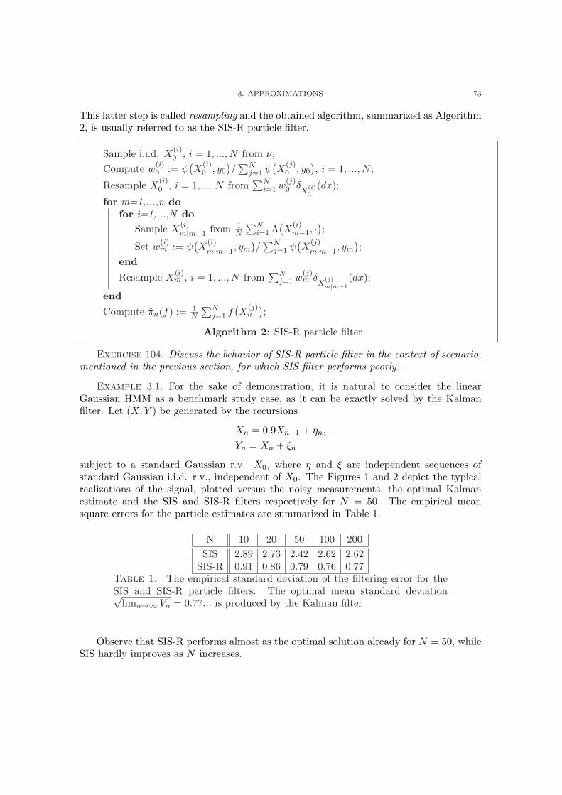
3. APPROXIMATIONS 73
This latter step is called resampling and the obtained algorithm, summarized as Algorithm2, is usually referred to as the SIS-R particle filter.
Sample i.i.d. X(i)0 , i = 1, ..., N from ν;
Compute w(i)0 := ψ
(X
(i)0 , y0
)/∑N
j=1 ψ(X
(j)0 , y0
), i = 1, ..., N ;
Resample X(i)0 , i = 1, ..., N from
∑Ni=1w
(j)0 δ
X(i)0
(dx);
for m=1,...,n dofor i=1,...,N do
Sample X(i)m|m−1 from 1
N
∑Ni=1 Λ
(X
(i)m−1, ·
);
Set w(i)m := ψ
(X
(i)m|m−1, ym
)/∑N
j=1 ψ(X
(j)m|m−1, ym
);
end
Resample X(i)m , i = 1, ..., N from
∑Nj=1w
(j)m δ
X(j)m|m−1
(dx);
end
Compute πn(f) :=1N
∑Nj=1 f
(X
(j)n
);
Algorithm 2: SIS-R particle filter
Exercise 104. Discuss the behavior of SIS-R particle filter in the context of scenario,mentioned in the previous section, for which SIS filter performs poorly.
Example 3.1. For the sake of demonstration, it is natural to consider the linearGaussian HMM as a benchmark study case, as it can be exactly solved by the Kalmanfilter. Let (X,Y ) be generated by the recursions
Xn = 0.9Xn−1 + ηn,
Yn = Xn + ξn
subject to a standard Gaussian r.v. X0, where η and ξ are independent sequences ofstandard Gaussian i.i.d. r.v., independent of X0. The Figures 1 and 2 depict the typicalrealizations of the signal, plotted versus the noisy measurements, the optimal Kalmanestimate and the SIS and SIS-R filters respectively for N = 50. The empirical meansquare errors for the particle estimates are summarized in Table 1.
N 10 20 50 100 200
SIS 2.89 2.73 2.42 2.62 2.62SIS-R 0.91 0.86 0.79 0.76 0.77
Table 1. The empirical standard deviation of the filtering error for theSIS and SIS-R particle filters. The optimal mean standard deviation√limn→∞ Vn = 0.77... is produced by the Kalman filter
Observe that SIS-R performs almost as the optimal solution already for N = 50, whileSIS hardly improves as N increases.

74 3. HIDDEN STATE ESTIMATION
0 10 20 30 40 50 60 70 80 90 100−8
−6
−4
−2
0
2
4
6
8
time
SIS particle approximation vs. the signal and the exact Kalman estimate
signalobservationKalmanSIS
Figure 1. SIS particle filter
0 10 20 30 40 50 60 70 80 90 100−2
−1
0
1
2
3
4
5
6
7
time
SIS−R particle approximation vs. the signal and the exact Kalman estimate
signalobservationKalmanSIS−R
Figure 2. SIS-R particle filter
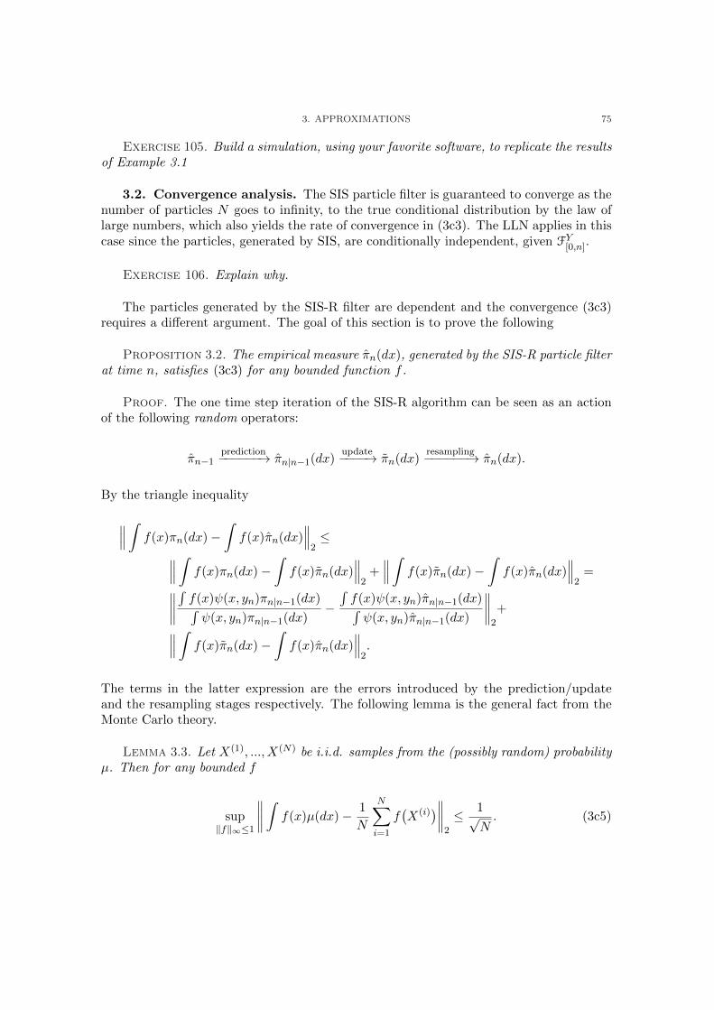
3. APPROXIMATIONS 75
Exercise 105. Build a simulation, using your favorite software, to replicate the resultsof Example 3.1
3.2. Convergence analysis. The SIS particle filter is guaranteed to converge as thenumber of particles N goes to infinity, to the true conditional distribution by the law oflarge numbers, which also yields the rate of convergence in (3c3). The LLN applies in thiscase since the particles, generated by SIS, are conditionally independent, given FY
[0,n].
Exercise 106. Explain why.
The particles generated by the SIS-R filter are dependent and the convergence (3c3)requires a different argument. The goal of this section is to prove the following
Proposition 3.2. The empirical measure πn(dx), generated by the SIS-R particle filterat time n, satisfies (3c3) for any bounded function f .
Proof. The one time step iteration of the SIS-R algorithm can be seen as an actionof the following random operators:
πn−1prediction−−−−−−→ πn|n−1(dx)
update−−−−→ πn(dx)resampling−−−−−−→ πn(dx).
By the triangle inequality
∥∥∥∫
f(x)πn(dx)−∫
f(x)πn(dx)∥∥∥2≤
∥∥∥∫
f(x)πn(dx)−∫
f(x)πn(dx)∥∥∥2+∥∥∥∫
f(x)πn(dx)−∫
f(x)πn(dx)∥∥∥2=
∥∥∥∥∫f(x)ψ(x, yn)πn|n−1(dx)∫ψ(x, yn)πn|n−1(dx)
−∫f(x)ψ(x, yn)πn|n−1(dx)∫ψ(x, yn)πn|n−1(dx)
∥∥∥∥2
+
∥∥∥∫
f(x)πn(dx)−∫
f(x)πn(dx)∥∥∥2.
The terms in the latter expression are the errors introduced by the prediction/updateand the resampling stages respectively. The following lemma is the general fact from theMonte Carlo theory.
Lemma 3.3. Let X(1), ..., X(N) be i.i.d. samples from the (possibly random) probabilityµ. Then for any bounded f
sup‖f‖∞≤1
∥∥∥∥∫
f(x)µ(dx)− 1
N
N∑
i=1
f(X(i)
)∥∥∥∥2
≤ 1√N
. (3c5)

76 3. HIDDEN STATE ESTIMATION
Proof. Since X(i), i = 1, ..., N are independent given µ,
E
(∫f(x)µ(dx)− 1
N
N∑
i=1
f(X(i)
))2
=
EE
((1
N
N∑
i=1
(f(X(i)
)−∫
f(x)µ(dx)))2∣∣∣µ
)=
1
N2EE
(∑
i,j
(f(X(i)
)−∫
f(x)µ(dx))(
f(X(j)
)−∫
f(x)µ(dx))∣∣∣µ
)=
1
N2EE
(Nvarµ(f)
∣∣∣µ)=
1
NEvarµ(f) ≤ ‖f‖2∞
1
N,
which implies the claimed bound. ¤
Resampling. Recall that πn(dx) is obtained by i.i.d. sampling from the (random) distri-bution πn(dx), and thus by Lemma 3.3,
∥∥∥∫
f(x)πn(dx)−∫
f(x)πn(dx)∥∥∥2≤ ‖f‖∞√
N.
Update. Using the elementary inequality
∣∣∣ac− b
d
∣∣∣ ≤ 1
|c|∣∣a− b
∣∣+∣∣∣ bdc
∣∣∣∣∣d− c
∣∣,
we obtain:
∣∣∣∣∫f(x)ψ(x, yn)πn|n−1(dx)∫ψ(x, yn)πn|n−1(dx)
−∫f(x)ψ(x, yn)πn|n−1(dx)∫ψ(x, yn)πn|n−1(dx)
∣∣∣∣ ≤
1∫ψ(x, yn)πn|n−1(dx)
∣∣∣∣∫
f(x)ψ(x, yn)πn|n−1(dx)−∫
f(x)ψ(x, yn)πn|n−1(dx)
∣∣∣∣+∫ |f(x)|ψ(x, yn)πn|n−1(dx)∫
ψ(x, yn)πn|n−1(dx)∫ψ(x, yn)πn|n−1(dx)
×∣∣∣∣∫
ψ(x, yn)πn|n−1(dx)−∫
ψ(x, yn)πn|n−1(dx)
∣∣∣∣ ≤‖fψ‖∞∫
ψ(x, yn)πn|n−1(dx)
∣∣∣∣∫
f1(x)πn|n−1(dx)−∫
f1(x)πn|n−1(dx)
∣∣∣∣+
‖f‖∞‖ψ‖∞∫ψ(x, yn)πn|n−1(dx)
∣∣∣∣∫
f2(x)πn|n−1(dx)−∫
f2(x)πn|n−1(dx)
∣∣∣∣,
(3c6)
with bounded f1(x) := f(x)ψ(x, yn)/‖fψ‖∞ and f2(x) := ψ(x, yn)/‖ψ‖∞.

3. APPROXIMATIONS 77
Prediction. Since πn|n−1(dx) is the empirical measure of i.i.d. samples from (πn−1Λ)(dx),once again, by the Lemma 3.3, for a bounded function g:
∥∥∥∥∫
g(x)πn|n−1(dx)−∫
g(x)πn|n−1(dx)
∥∥∥∥2
≤∥∥∥∥∫
g(x)(πn−1Λ
)(dx)−
∫g(x)
(πn−1Λ
)(dx)
∥∥∥∥2
+
∥∥∥∥∫
g(x)(πn−1Λ
)(dx)−
∫g(x)πn|n−1(dx)
∥∥∥∥2
≤
‖Λg‖∞ sup‖f‖∞≤1
∥∥∥∥∫
f(x)πn−1(dx)−∫
f(x)πn−1(dx)
∥∥∥∥2
+‖g‖∞√
N≤ ‖g‖∞
(∆n +
1√N
)
where we set
∆n := sup‖f‖∞≤1
∥∥∥∫
f(x)πn(dx)−∫
f(x)πn(dx)∥∥∥2.
Letting
Dn :=2‖ψ‖∞∫
ψ(x, yn)πn|n−1(dx), (3c7)
and assembling all parts together, we obtain the inequalities:
∆n ≤ Dn
(∆n−1 +
1√N
)+
1√N
, (3c8)
and (∆n +
1√N
)≤ Dn
(∆n−1 +
1√N
)+
2√N
,
which implies
Dn ≤( n∏
m=1
Dm
)∆0 +
2√N
n∑
`=1
( n∏
m=`
Dm
).
Finally, by similar calculations one verifies the bound
∆0 ≤ 1√N
(1 +
2‖ψ‖∞∫ψ(x, y0)ν(dx)
). (3c9)
Hence for a constant cn,
∥∥∥∫
f(x)πn(dx)−∫
f(x)πn(dx)∥∥∥2≤ cn
‖f‖∞√N
.
¤
Exercise 107. Verify the bound (3c9).
3.3. Other approaches. Many other approximation techniques are available, typi-cally fitting into one of the following categories:
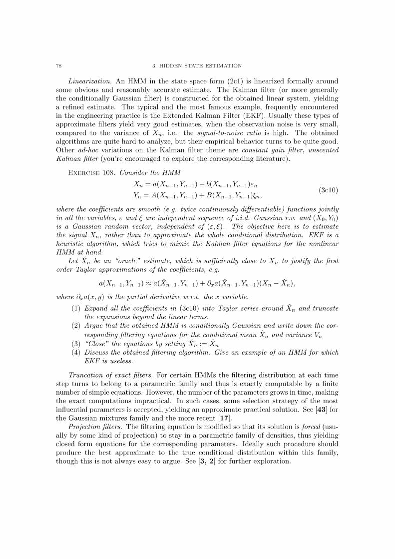
78 3. HIDDEN STATE ESTIMATION
Linearization. An HMM in the state space form (2c1) is linearized formally aroundsome obvious and reasonably accurate estimate. The Kalman filter (or more generallythe conditionally Gaussian filter) is constructed for the obtained linear system, yieldinga refined estimate. The typical and the most famous example, frequently encounteredin the engineering practice is the Extended Kalman Filter (EKF). Usually these types ofapproximate filters yield very good estimates, when the observation noise is very small,compared to the variance of Xn, i.e. the signal-to-noise ratio is high. The obtainedalgorithms are quite hard to analyze, but their empirical behavior turns to be quite good.Other ad-hoc variations on the Kalman filter theme are constant gain filter, unscentedKalman filter (you’re encouraged to explore the corresponding literature).
Exercise 108. Consider the HMM
Xn = a(Xn−1, Yn−1) + b(Xn−1, Yn−1)εn
Yn = A(Xn−1, Yn−1) +B(Xn−1, Yn−1)ξn,(3c10)
where the coefficients are smooth (e.g. twice continuously differentiable) functions jointlyin all the variables, ε and ξ are independent sequence of i.i.d. Gaussian r.v. and (X0, Y0)is a Gaussian random vector, independent of (ε, ξ). The objective here is to estimatethe signal Xn, rather than to approximate the whole conditional distribution. EKF is aheuristic algorithm, which tries to mimic the Kalman filter equations for the nonlinearHMM at hand.
Let Xn be an “oracle” estimate, which is sufficiently close to Xn to justify the firstorder Taylor approximations of the coefficients, e.g.
a(Xn−1, Yn−1) ≈ a(Xn−1, Yn−1) + ∂xa(Xn−1, Yn−1)(Xn − Xn),
where ∂xa(x, y) is the partial derivative w.r.t. the x variable.
(1) Expand all the coefficients in (3c10) into Taylor series around Xn and truncatethe expansions beyond the linear terms.
(2) Argue that the obtained HMM is conditionally Gaussian and write down the cor-
responding filtering equations for the conditional mean Xn and variance Vn
(3) “Close” the equations by setting Xn := Xn
(4) Discuss the obtained filtering algorithm. Give an example of an HMM for whichEKF is useless.
Truncation of exact filters. For certain HMMs the filtering distribution at each timestep turns to belong to a parametric family and thus is exactly computable by a finitenumber of simple equations. However, the number of the parameters grows in time, makingthe exact computations impractical. In such cases, some selection strategy of the mostinfluential parameters is accepted, yielding an approximate practical solution. See [43] forthe Gaussian mixtures family and the more recent [17].
Projection filters. The filtering equation is modified so that its solution is forced (usu-ally by some kind of projection) to stay in a parametric family of densities, thus yieldingclosed form equations for the corresponding parameters. Ideally such procedure shouldproduce the best approximate to the true conditional distribution within this family,though this is not always easy to argue. See [3, 2] for further exploration.

4. FILTER STABILITY 79
Small noise approximations. In good engineering systems the observation noise is smallcompared to the signal amplitude. In these cases the filtering distribution concentratesaround the true value of the signal and can be approximated asymptotically as the noiseintensity vanishes. Such approximations yield practical filters with optimal error asymp-totic: see [25, 24], [38, 37].
Weak convergence approximations. In many practical situations HMMs behave sta-tistically as other HMMs, with simpler structure, appropriate for construction of exactfilters, which can be applied to the original observations and still yield reasonably goodestimates. For example, a linear system with “almost” Gaussian noises would not admitan exact f.d.f., though it is intuitively clear that the Kalman filter would generate a goodapproximate solution. The general approach to such problems has been developed withinthe framework of weak convergence of random processes (see e.g. [27], [28], [12], [32],[26], [18]).
4. Filter stability
In the previous section we saw that SIS-R algorithm satisfies the bound (3c3) foreach fixed time n ≥ 1. However, it is clear from the proof that the constants cn maygrow exponentially in n and hence, essentially, Proposition 3.2 does not guarantee anyimprovement of SIS-R over the naive SIS. On the other hand, the experiments as theExample 3.1 indicate that SIS-R performance does not tend to degrade with time andapparently the claim of Proposition 3.2 is far from being the optimal result.
Let us show what the origin of the better behavior could possibly be. Recall that thefiltering distribution πn satisfies the recursive equation πn = Fn πn−1, subject to π0 = ν,where Fn stands for the operator acting on probability measures, defined by the righthand side of (3a1), i.e.
(Fn µ)(dx) := ψ(x, yn)∫Λ(x′, dx)µ(dx′)∫
ψ(x, yn)∫Λ(x′, dx)µ(dx′)
, µ ∈ P(E1).
Similarly, πn generated by the SIS-R particle filter, is given by πNn = FN
n πNn−1, subject to
π0 = ν, where FNn is a random operator, acting on probability measures (more precisely,
purely atomic probability measures), defined by the Algorithm 2.
The inequality (3c8) means that the operator FNn approximates the operator Fn in
the sense∥∥Fn µ− FN
n µ∥∥2:= sup
‖f‖∞≤1
∥∥∥(Fn µ)(f)− (
FNn µ)(f)
∥∥∥2=
sup‖f‖∞≤1
√E∣∣∣(Fn µ)(f)− (
FNn µ)(f)
∣∣∣2≤ C√
N, (3d1)
for a probability measure µ. If we assume that
κ ≤ ψ(x, y) ≤ κ−1, (3d2)
for all x and y and a constant κ > 0, then by (3c7) the constant C := 1+κ2 can be chosen.
Exercise 109. Explain why (3c8) yields (3d1).

80 3. HIDDEN STATE ESTIMATION
By the triangle inequality,
∥∥πn − πNn
∥∥2=
∥∥∥∥Fn ... F1 ν − FNn ... FN
1 ν∥∥∥∥2∥∥∥∥
n∑
m=1
Fn ... Fm+1 Fm πNm−1 − Fn ... Fm+1 FN
m πNm−1
∥∥∥∥2
≤n∑
m=1
∥∥∥Fn ... Fm+1 Fm πNm−1 − Fn ... Fm+1 FN
m πNm−1
∥∥∥2.
Suppose we manage to show that for a pair of measures µ and ν,∥∥∥Fn ... Fm+1 µ− Fn ... Fm+1 ν
∥∥∥2≤ cγn−m‖µ− ν‖2, (3d3)
for some positive constants c and γ < 1. Then in view of (3d1)
∥∥πn − πNn
∥∥2≤
n∑
m=1
cγn−m‖Fm πNm−1 − FN
m πNm−1‖2 ≤
n∑
m=1
cγn−mC1√N
≤ cC
1− γ
1√N
.
In words, if the exact optimal filter forgets its initial condition exponentially fast, then thelocal approximation errors do not accumulate and consequently the approximation errorhas the order 1/
√N uniformly over time. This is a tremendous improvement and practical
advantage over the naive bound (3c3)!It is left to verify the key property (3d3). Let us start with the following useful result.
Lemma 4.1. Let Λ be a Markov kernel, such that for some ε > 0 and a probabilitymeasure ρ
Λ(x,A) ≥ ερ(A), ∀x ∈ E1, A ∈ E1. (3d4)
Then
‖Λ µ1 − Λ µ2‖2 ≤ (1− ε)‖µ1 − µ2‖2. (3d5)
Remark 4.2. The assumption (3d4) is called the Doeblin condition, after the famousprobabilist Wolfgang Doeblin, who perished in WWII.
Proof. Define
Λ(x, dx′) :=1
1− ε
Λ(x, dx′)− ερ(dx′)
.
Clearly, Λ(x, dx′) is a Markov probability kernel, as it is nonnegative by (3d4) and inte-grates to one for all x ∈ E1. Moreover, for any bounded f :
(Λ µ1
)(f)− (
Λ µ2
)(f) = (1− ε)
(Λ µ1
)(f)− (
Λ µ2
)(f)
,
and thus∣∣∣(Λ µ1
)(f)− (
Λ µ2
)(f)
∣∣∣ = (1− ε)∣∣∣(Λ µ1
)(f)− (
Λ µ2
)(f)
∣∣∣ = (1− ε)∣∣µ1(g)− µ2(g)
∣∣

4. FILTER STABILITY 81
where g(u) :=∫f(v)Λ(u, dv). Note that ‖g‖∞ ≤ ‖f‖∞ and hence
∥∥∥Λ µ1 − Λ µ2
∥∥∥2
2= sup
‖f‖∞≤1E((
Λ µ1
)(f)− (
Λ µ2
)(f)
)2≤
(1− ε)2 sup‖g‖∞≤1
E(µ1(g)− µ2(g)
)2= (1− ε)2
∥∥µ1 − µ2
∥∥22.
¤
This lemma is not directly applicable to the operators Fn, as they are not linear integraloperators, associated with a Markov kernel 14. The trick is to use the conditional Markovproperty of the signal. By Exercise 79,
πk+1|n(A) =∫
AΛk|n(x, dx′)πk|n(dx), k = m, ..., n− 1 (3d6)
where
Λk|n(x,A) =
∫A βk|n(x′)ψ(x′, Yk)Λ(x, dx′)∫E1
βk|n(x′)ψ(x′, Yk)Λ(x, dx′), (3d7)
and βm|n, ..., βn|n solve the backward equation
βk|n(x) =∫
ψ(u, Yk+1)βk+1|n(u)Λ(x, du), k = m, ..., n− 1,
subject to βn|n(x) ≡ 1. Consequently, n > m
Fn ... Fm+1 µ = Λn|n ... Λm+1|n µm|n, (3d8)
where
µm|n(A) =
∫A βm|n(x)µ(dx)∫E1
βm|n(x)µ(dx). (3d9)
This replaces the nonlinear dynamics by the linear one, suitable for application of theLemma 4.1.
Theorem 4.3. Assume that the signal kernel Λ(x, dx′) satisfies the strong mixingcondition: for some ε > 0 and a probability measure ρ,
ερ(A) ≤ Λ(x,A) ≤ 1
ερ(A), ∀x ∈ E1, ∀A ∈ E1. (3d10)
Then (3d3) holds with
c := 2/ε2, γ := 1− ε2.
Remark 4.4. The claim of this theorem remains valid, if ρ(A) is a σ-finite measure,rather than a probability measure.
14in fact, they are positive projective operators, which can be exploited to verify stability in a differentway, using tools from functional analysis
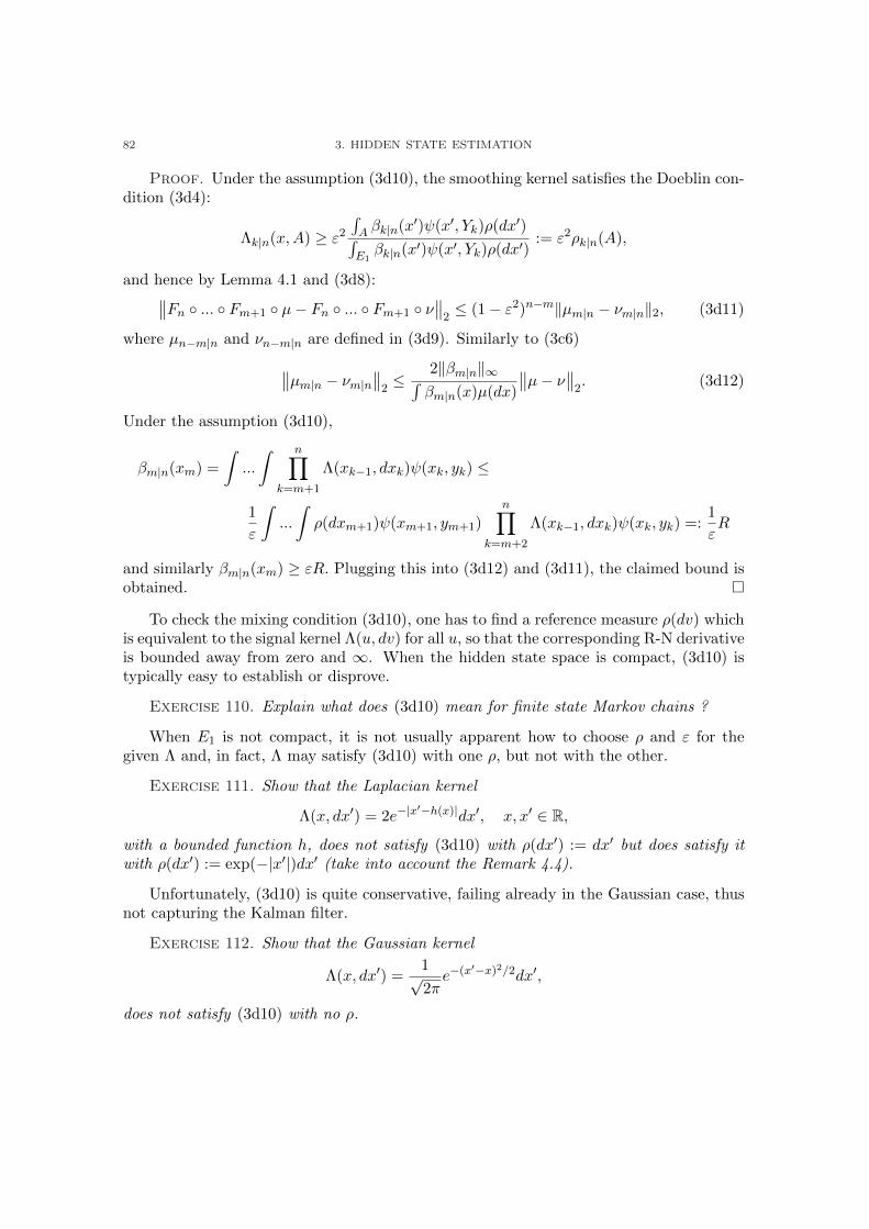
82 3. HIDDEN STATE ESTIMATION
Proof. Under the assumption (3d10), the smoothing kernel satisfies the Doeblin con-dition (3d4):
Λk|n(x,A) ≥ ε2∫A βk|n(x′)ψ(x′, Yk)ρ(dx′)∫E1
βk|n(x′)ψ(x′, Yk)ρ(dx′):= ε2ρk|n(A),
and hence by Lemma 4.1 and (3d8):∥∥Fn ... Fm+1 µ− Fn ... Fm+1 ν
∥∥2≤ (1− ε2)n−m‖µm|n − νm|n‖2, (3d11)
where µn−m|n and νn−m|n are defined in (3d9). Similarly to (3c6)
∥∥µm|n − νm|n∥∥2≤ 2‖βm|n‖∞∫
βm|n(x)µ(dx)∥∥µ− ν
∥∥2. (3d12)
Under the assumption (3d10),
βm|n(xm) =
∫...
∫ n∏
k=m+1
Λ(xk−1, dxk)ψ(xk, yk) ≤
1
ε
∫...
∫ρ(dxm+1)ψ(xm+1, ym+1)
n∏
k=m+2
Λ(xk−1, dxk)ψ(xk, yk) =:1
εR
and similarly βm|n(xm) ≥ εR. Plugging this into (3d12) and (3d11), the claimed bound isobtained. ¤
To check the mixing condition (3d10), one has to find a reference measure ρ(dv) whichis equivalent to the signal kernel Λ(u, dv) for all u, so that the corresponding R-N derivativeis bounded away from zero and ∞. When the hidden state space is compact, (3d10) istypically easy to establish or disprove.
Exercise 110. Explain what does (3d10) mean for finite state Markov chains ?
When E1 is not compact, it is not usually apparent how to choose ρ and ε for thegiven Λ and, in fact, Λ may satisfy (3d10) with one ρ, but not with the other.
Exercise 111. Show that the Laplacian kernel
Λ(x, dx′) = 2e−|x′−h(x)|dx′, x, x′ ∈ R,with a bounded function h, does not satisfy (3d10) with ρ(dx′) := dx′ but does satisfy itwith ρ(dx′) := exp(−|x′|)dx′ (take into account the Remark 4.4).
Unfortunately, (3d10) is quite conservative, failing already in the Gaussian case, thusnot capturing the Kalman filter.
Exercise 112. Show that the Gaussian kernel
Λ(x, dx′) =1√2π
e−(x′−x)2/2dx′,
does not satisfy (3d10) with no ρ.

4. FILTER STABILITY 83
On the other hand, the Kalman filter is well known to be stable under very generalconditions. The proof of this fact, uses the special structure of the filter and in particularthe convergence properties of the Riccati equation15.
Exercise 113. Use the explicit form of the equations to find conditions under whichthe Kalman filter from Theorem 2.9 is stable (in any reasonable sense).
Various weaker forms of stability of the filtering equation can be established underweaker conditions (see e.g. the recent survey [8]).
15or, alternatively, the dual control problem


CHAPTER 4
Inference
1. Generalities
Up to now we assumed that the HMM is completely specified, i.e. that the triplet(Λ, ψ, ν) is known. In this chapter we shall address the problem of parameter estimationfor HMMs in the following classical statistical setting. Let Θ ⊆ Rd and suppose that theHMM is specified up to an unknown parameter θ ∈ Θ. In other words, we are given asample from an HMM, corresponding to one of the members of the parametric family(Λθ, ψθ, νθ), θ ∈ Θ and would like to estimate the parameter θ.
We shall focus below on the Maximum Likelihood Estimators (MLE), which constitutemuch of the literature on the subject up to the date. Let us briefly recall the MLEbasics. Suppose we are given a parametric family of probability measures Pθ, θ ∈ Θ ⊆ Rd
on a measurable space (E,E), all of which are absolutely continuous with respect to a
fixed reference σ-finite measure Υ with the R-N densities dPθdΥ (x) := Lθ(x). The function
θ 7→ Lθ(x) is called the likelihood function. The MLE is defined as a maximizer of thelikelihood with respect to θ ∈ Θ, evaluated at the obtained observation X, namely it is arandom variable θ with values in Θ, such that
Lθ(X) = supθ∈Θ
Lθ(X). (4a1)
This definition makes sense if e.g. we assume that Lθ(x) is a continuous function in θ for
each x ∈ E and Θ is compact. Notice that θ need not have to be unique and in the caseof ambiguity any maximizer θ is taken. This is one of the oldest estimation techniques,dating back to D.Bernoulli.
Exercise 114. Show that the definition (4a1) does not depend on the reference measureΥ, i.e. that for any two distinct reference measures the same MLE is obtained.
Technically the MLE procedure reduces to global maximization of the likelihood Lθ(X)over Θ. Sometimes the maximization problem can be solved explicitly, but in most prac-tical situations is computed numerically.
Many statistical problems naturally depend on an auxiliary index, which can be con-trolled by the statistician. One commonly encountered example1 is the large sample as-ymptotic setting, when a large number n of i.i.d. samples are available. Obviously theaccuracy of a good estimation procedure should improve as n increases and should esti-mate θ precisely, asymptotically as n → ∞, in which case the estimate is called consistent,
1other examples are high signal-to-noise ratio, or the dimension of the data, etc.
85

86 4. INFERENCE
i.e. for all ε > 0,
limn→∞Pθ0
(|θn − θ0| ≥ ε)= 0, ∀θ0 ∈ Θ, (4a2)
where θ0 stands for the true unknown value of the parameter and the subscript n in θnemphasizes its dependence on n.
The sequence of consistent estimators (θn) is said to have asymptotic distribution µθ0
at rate rn ∞, if the normalized sequence of estimation errors converges in distributionto µθ0 under Pθ0 :
rn(θn − θ0)d−−−→
n→∞ µθ, under Pθ0 .
Under certain regularity conditions the sequence of MLE’s is asymptotically normal withzero mean and variance 1/I(θ0), where I(θ0) is the Fisher information. Moreover it isasymptotically efficient in an appropriate sense, i.e. cannot be essentially improved (con-sult e.g. the text [20]).
To summarize, the two main aspects of a parameter estimation problem is the com-putational one, i.e. suggesting an efficient procedure for calculating the estimate, and theanalytical one, i.e. the performance analysis of the proposed estimate.
Let us now see how does the MLE look like for HMMs. In view of (2c7), the naturalcandidate for the reference measure is Υ(dy0 × ...× dyn) := δ0(dy0)×Ψ(y1)× ...×Ψ(dyn)and the corresponding likelihood is2
Lθ(yn) = Eθ
n∏
m=1
ψθ
(Xm, ym
)=
Eθ
Eθ
(ψθ
(Xn, yn
)|FX[0,n−1]
) n−1∏
m=1
ψθ
(Xm, ym
)=
∫ψθ(xn, yn)π
θn|n−1(dxn)Eθ
n−1∏
m=1
ψθ
(Xm, ym
)= ... =
∫νθ(dx0)
n∏
m=1
∫ψθ(xm, ym)πθ
m|m−1(dxm), (4a3)
where πθm|m−1(dxm) =
∫Λθ(xm−1, dxm)πθ
m−1(dxm−1) and πθm−1 is the solution of the
filtering equation (3a1) (depending on θ!).
Hence calculating the MLE θn amounts to finding the global maximum of Lθ(yn), using
any suitable optimization technique. For example, one may use one of the steepest descenttype optimization algorithms, etc. It turns out, however, that the special structure of theproblem admits a more elegant “native” method, namely the Expectation-Maximization(EM) algorithm, described in the next section.
2. The EM algorithm
The EM algorithm is an iterative procedure, which starts from an initial guess of theparameter and produces a sequence of estimates in Θ, along which the likelihood function
2Once again, we assume positive ψ(x, y) and use the notation yn = (y1, ..., yn)

2. THE EM ALGORITHM 87
does not decrease. EM is a general technique suitable for problems with incomplete data,such as in the case of HMM setting.
The idea can be demonstrated already in the following simplest setting. Suppose(X,Y ) is a pair of real random variables with the probability density fθ(x, y) depending onthe parameter θ ∈ Θ. The pair is viewed as the complete data, unavailable to statistician.The estimate of θ is to be based only on the observation of Y , the incomplete data. Thestraightforward calculation of the MLE reduces in this case to the maximization of thelog-likelihood of Y :
logLθ(y) := log fθ(y) = log
∫fθ(x, y)dx. (4b1)
This optimization can be quite hard, especially when the dimensions of the integrationand/or optimization domains are high.
Instead, for any fixed point θ′ in Θ the very same answer will be obtained if wemaximize w.r.t. θ ∈ Θ the log-likelihood function (recall Exercise 114):
logL(θ, θ′; y) = logfθ(y)
fθ′(y)= log
∫fθ(x, y)dx∫fθ′(x, y)dx
=
log
∫fθ(x, y)
fθ′(x, y)
fθ′(x, y)∫fθ′(x, y)dx
dx =
log
∫fθ(x, y)
fθ′(x, y)fθ′(x|y)dx = log Eθ′
(fθ(X,Y )
fθ′(X,Y )
∣∣∣Y = y
)
where fθ′(x|y) is the conditional probability density of X given Y under parameter θ′ andfθ(x, y)/fθ′(x, y) is the likelihoods ratio of the complete data. Define
Q(θ, θ′) := Eθ′
(log
fθ(X,Y )
fθ′(X,Y )
∣∣∣Y),
and let θ′′ be the maximizer of Q(θ; θ′) over θ ∈ Θ. Since Q(θ′, θ′) = 0, obviouslyQ(θ′′, θ′) ≥ 0 and by the Jensen inequality
logLθ′′(Y )− logLθ′(Y ) = logL(θ′′, θ′;Y ) =
log Eθ′
(fθ′′(X,Y )
fθ′(X,Y )
∣∣∣Y)
≥ Eθ′
(log
fθ′′(X,Y )
fθ′(X,Y )
∣∣∣Y)
= Q(θ′′, θ′) ≥ 0.
The latter means that the value of the log-likelihood function logLθ(Y ) does not decrease,when θ′ is replaced with θ′′. Hence if we start with some initial guess of the parameterθ(0) ∈ Θ and set θ(i) to be a maximizer of Q(θ; θ(i−1)) over θ ∈ Θ, we obtain a sequence of
estimators θ(i), i ≥ 0 along which the log-likelihood does not decrease. The calculation ofthe conditional expectation Q(θ, θ′) is called the E-step and its maximization with respectto θ is referred to as the M-step.
Notice that the function Q(θ; θ′) is the conditional expectation of a specific function ofX (and Y ), given Y and in many concrete situations admits a closed form simple formula(without a need to calculate complicated integrals on each iterate). Moreover, often themaximization of Q(θ, θ′) can also be carried out explicitly, yielding a simple iterativeprocedure.
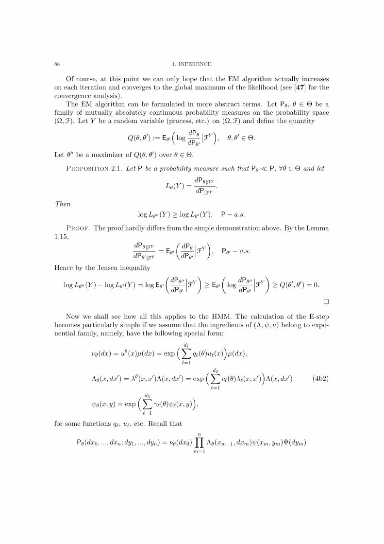
88 4. INFERENCE
Of course, at this point we can only hope that the EM algorithm actually increaseson each iteration and converges to the global maximum of the likelihood (see [47] for theconvergence analysis).
The EM algorithm can be formulated in more abstract terms. Let Pθ, θ ∈ Θ be afamily of mutually absolutely continuous probability measures on the probability space(Ω,F). Let Y be a random variable (process, etc.) on (Ω,F) and define the quantity
Q(θ, θ′) := Eθ′(log
dPθ
dPθ′
∣∣FY), θ, θ′ ∈ Θ.
Let θ′′ be a maximizer of Q(θ, θ′) over θ ∈ Θ.
Proposition 2.1. Let P be a probability measure such that Pθ ¿ P, ∀θ ∈ Θ and let
Lθ(Y ) =dPθ |FY
dP|FY
.
Then
logLθ′′(Y ) ≥ logLθ′(Y ), P− a.s.
Proof. The proof hardly differs from the simple demonstration above. By the Lemma1.15,
dPθ |FY
dPθ′ |FY
= Eθ′
(dPθ
dPθ′
∣∣∣FY
), Pθ′ − a.s.
Hence by the Jensen inequality
logLθ′′(Y )− logLθ′(Y ) = log Eθ′
(dPθ′′
dPθ′
∣∣∣FY
)≥ Eθ′
(log
dPθ′′
dPθ′
∣∣∣FY
)≥ Q(θ′, θ′) = 0.
¤
Now we shall see how all this applies to the HMM. The calculation of the E-stepbecomes particularly simple if we assume that the ingredients of (Λ, ψ, ν) belong to expo-nential family, namely, have the following special form:
νθ(dx) = uθ(x)µ(dx) = exp( d1∑
`=1
q`(θ)u`(x))µ(dx),
Λθ(x, dx′) = λθ(x, x′)Λ(x, dx′) = exp
( d2∑
`=1
c`(θ)λ`(x, x′))Λ(x, dx′)
ψθ(x, y) = exp( d3∑
`=1
γ`(θ)ψ`(x, y)),
(4b2)
for some functions q`, u`, etc. Recall that
Pθ(dx0, ..., dxn; dy1, ..., dyn) = νθ(dx0)
n∏
m=1
Λθ(xm−1, dxm)ψ(xm, ym)Ψ(dym)

2. THE EM ALGORITHM 89
and thus for the exponential model (4b2), the likelihood of the complete data reads
logdPθ
dPθ′(xn, yn) =
d1∑
`=1
(q`(θ)− q`(θ
′))u`(x)+
n∑
m=1
d2∑
`
(c`(θ)− c`(θ
′))λ`(xm−1, xm) +
n∑
m=1
d3∑
`
(γ`(θ)− γ`(θ
′))ψ(xm, ym)
Then
Qn(θ, θ′) = Eθ′
log
dPθ
dPθ′
∣∣∣FY[0,n]
=
d1∑
`=1
(q`(θ)− q`(θ
′))∫
u`(x)πθ′0|n(dx)+
d2∑
`
(c`(θ)− c`(θ
′)) n∑
m=1
∫λ`(x, x
′)πθ′m−1,m|n(dx, dx
′)
+
d3∑
`
(γ`(θ)− γ`(θ
′)) n∑
m=1
∫ψ(x, Ym)πθ′
m|n(dx),
where the integrators are the appropriate smoothing distributions, which can be generatedby various algorithms, presented in the previous chapter. Notice that the maximizationw.r.t. θ of Qn(θ, θ
′), required by theM -step, is simpler than of the original likelihood (4a3)(where the optimization argument appeared in the smoothing distributions themselves!).
Let us demonstrate the ideas by the following classical example:
Example 2.2 (the Baum-Welch algorithm). LetX be a finite Markov chain with valuesin E1 = 1, ..., d, transition probabilities λij and the initial probabilities νj . Suppose thechain is observed in the white Gaussian noise
Yn = h(Xn) +√g(Xn)ξn, n ≥ 1,
where ξ is a sequence of standard Gaussian random variables. The objective is to estimateθ =
(ν,Λ, h, g
), where the function h and g are treated as the vectors of the corresponding
values at the points of E1. The parameter space Θ can be chosen to be the subset of theusual Euclidian space, which naturally embeds all the quantities with all the constraints(i.e. positivity of ν and λij ,
∑j λij = 1, etc.) We shall also assume for simplicity that
λij > 0 and νi > 0 for all i and j, so that the chain fits the exponential family:
Λθ(x, dx′) = exp
( d∑
k,`=1
log(λk`d)1k=x1`=x′)1d
d∑
k=1
δk(dx′)
and
νθ(dx) = exp( d∑
i=1
log(νid)1x=i)1d
d∑
k=1
δk(dx).
Also
ψθ(x, y) = exp
d∑
i=1
1x=i
(− 1
2log
(2πg(i)
)−(y − h(i)
)22g(i)
).
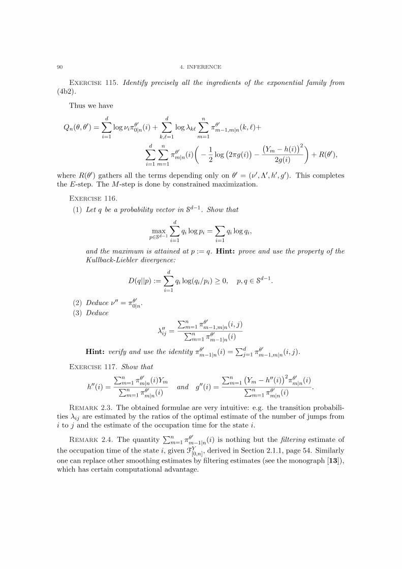
90 4. INFERENCE
Exercise 115. Identify precisely all the ingredients of the exponential family from(4b2).
Thus we have
Qn(θ, θ′) =
d∑
i=1
log νiπθ′0|n(i) +
d∑
k,`=1
log λk`
n∑
m=1
πθ′m−1,m|n(k, `)+
d∑
i=1
n∑
m=1
πθ′m|n(i)
(− 1
2log
(2πg(i)
)−(Ym − h(i)
)22g(i)
)+R(θ′),
where R(θ′) gathers all the terms depending only on θ′ = (ν ′,Λ′, h′, g′). This completesthe E-step. The M -step is done by constrained maximization.
Exercise 116.
(1) Let q be a probability vector in Sd−1. Show that
maxp∈Sd−1
d∑
i=1
qi log pi =∑
i=1
qi log qi,
and the maximum is attained at p := q. Hint: prove and use the property of theKullback-Liebler divergence:
D(q||p) :=d∑
i=1
qi log(qi/pi) ≥ 0, p, q ∈ Sd−1.
(2) Deduce ν ′′ = πθ′0|n.
(3) Deduce
λ′′ij =
∑nm=1 π
θ′m−1,m|n(i, j)∑n
m=1 πθ′m−1|n(i)
Hint: verify and use the identity πθ′m−1|n(i) =
∑dj=1 π
θ′m−1,m|n(i, j).
Exercise 117. Show that
h′′(i) =
∑nm=1 π
θ′m|n(i)Ym∑n
m=1 πθ′m|n(i)
and g′′(i) =
∑nm=1
(Ym − h′′(i)
)2πθ′m|n(i)∑n
m=1 πθ′m|n(i)
.
Remark 2.3. The obtained formulae are very intuitive: e.g. the transition probabili-ties λij are estimated by the ratios of the optimal estimate of the number of jumps fromi to j and the estimate of the occupation time for the state i.
Remark 2.4. The quantity∑n
m=1 πθ′m−1|n(i) is nothing but the filtering estimate of
the occupation time of the state i, given FY[0,n], derived in Section 2.1.1, page 54. Similarly
one can replace other smoothing estimates by filtering estimates (see the monograph [13]),which has certain computational advantage.

2. THE EM ALGORITHM 91
Guess θ′ := (ν,Λ, h, g);repeat
Compute πθ′m−1,m|n by the forward-backward recursions;
Compute νi := πθ′0|n(i), i = 1, ..., d;
Compute λij :=∑n
m=1 πθ′m−1,m|n(i, j)/
∑nm=1 π
θ′m−1|n(i);
Compute h(i) :=∑n
m=1 πθ′m|n(i)Ym/
∑nm=1 π
θ′m|n(i);
Compute g(i) :=∑n
m=1
(Ym − h′′(i)
)2πθ′m|n(i)/
∑nm=1 π
θ′m|n(i);
Set θ′ := (ν,Λ, h, g)until convergence stopping rule holds ;
Algorithm 3: The Baum-Welch algorithm
Exercise 118. Build a simulation of the Baum-Welch algorithm using your favoritesoftware. Study its performance empirically.
Exercise 119. Derive the EM algorithm for the linear Gaussian HMM:
Xn = aXn−1 + bεn
Yn = AXn−1 +Bξn
to estimate the parameter θ = (a, b, A,B). Discuss the obtained equations.
Remark 2.5. In the latter exercise the smoothing distributions are Gaussian andclosed form recursions can be derived for their means and variances (Kalman smoothers).


Bibliography
[1] Petrie T. P. Soules G. Baum, L. E. and N. Weiss. A maximization technique occurring in the statisticalanalysis of probabilistic functions of markov chains. Ann. Math. Statist., 41:164171, 1970.
[2] Damiano Brigo, Bernard Hanzon, and Francois Le Gland. Approximate nonlinear filtering by projec-tion on exponential manifolds of densities. Bernoulli, 5(3):495–534, 1999.
[3] Damiano Brigo, Bernard Hanzon, and Francois LeGland. A differential geometric approach to non-linear filtering: the projection filter. IEEE Trans. Automat. Control, 43(2):247–252, 1998.
[4] R. W. Brockett and J. M. C. Clark. The geometry of the conditional density equation. In Analysisand optimisation of stochastic systems (Proc. Internat. Conf., Univ. Oxford, Oxford, 1978), pages299–309. Academic Press, London, 1980.
[5] Amke Caliebe. Properties of the maximum a posteriori path estimator in hidden markov models.IEEE Trans. on Inf. Theory, 52(1):41–51, January 2006.
[6] Amke Caliebe and Uwe Rosler. Convergence of the maximum a posteriori path estimator in hiddenmarkov models. IEEE Trans. on Inf. Theory, 48(7):1750–1758, July 2002.
[7] Olivier Cappe, Eric Moulines, and Tobias Ryden. Inference in hidden Markov models. Springer Seriesin Statistics. Springer, New York, 2005. With Randal Douc’s contributions to Chapter 9 and ChristianP. Robert’s to Chapters 6, 7 and 13, With Chapter 14 by Gersende Fort, Philippe Soulier and Moulines,and Chapter 15 by Stephane Boucheron and Elisabeth Gassiat.
[8] P. Chigansky, R. Liptser, and R. van Handel. Intrinsic methods in filter stability. In Handbook ofNonlinear Filtering. Oxford University Press, 2011.
[9] Frederick E. Daum. Exact finite-dimensional nonlinear filters. IEEE Trans. Automat. Control,31(7):616–622, 1986.
[10] Luc Devroye. Nonuniform random variate generation. Springer-Verlag, New York, 1986.[11] G. B. Di Masi, P. Kitsul, and R. Sh. Liptser. Minimal dimension linear filters for stationary Markov
processes with finite state space. Stochastics Stochastics Rep., 36(1):1–19, 1991.[12] G. B. Di Masi, W. J. Runggaldier, and B. Armellin. On recursive approximations with error bounds
in nonlinear filtering. In Stochastic optimization (Kiev, 1984), volume 81 of Lecture Notes in Controland Inform. Sci., pages 127–135. Springer, Berlin, 1986.
[13] Robert J. Elliott, Lakhdar Aggoun, and John B. Moore. Hidden Markov models, volume 29 of Appli-cations of Mathematics (New York). Springer-Verlag, New York, 1995. Estimation and control.
[14] Yariv Ephraim and Neri Merhav. Hidden Markov processes. IEEE Trans. Inform. Theory, 48(6):1518–1569, 2002. Special issue on Shannon theory: perspective, trends, and applications.
[15] Marco Ferrante and Paolo Vidoni. Finite-dimensional filters for nonlinear stochastic difference equa-tions with multiplicative noises. Stochastic Process. Appl., 77(1):69–81, 1998.
[16] Marco Ferrante and Paolo Vidoni. A Gaussian-generalized inverse Gaussian finite-dimensional filter.Stochastic Process. Appl., 84(1):165–176, 1999.
[17] Valentine Genon-Catalot. A non-linear explicit filter. Statist. Probab. Lett., 61(2):145–154, 2003.[18] Eimear M. Goggin. Convergence in distribution of conditional expectations. Ann. Probab., 22(2):1097–
1114, 1994.[19] N.J. Gordon, D. Salmond, and A.F.M. Smith. Novel approach to nonlinear/non-gaussian bayesian
state estimation. Radar and Signal Processing, IEE Proceedings F, 140(2):107 – 113, 1993.[20] I. A. Ibragimov and R. Z. Has′minskiı. Statistical estimation, volume 16 of Applications of Mathe-
matics. Springer-Verlag, New York, 1981. Asymptotic theory, Translated from the Russian by SamuelKotz.
93

94 BIBLIOGRAPHY
[21] T. Kailath, A.H. Sayed, and B. Hassibi. Linear Estimation. Prentice Hall Information and SystemSciences Series. Prentice Hall, 2000.
[22] R. E. Kalman and R. S. Bucy. New results in linear filtering and prediction theory. Trans. ASME Ser.D. J. Basic Engrg., 83:95–108, 1961.
[23] R.E. Kalman. A new approach to linear filtering and prediction problems. Journal of Basic Engineer-ing, 82(1):3545, 1960.
[24] R. Katzur, B. Z. Bobrovsky, and Z. Schuss. Asymptotic analysis of the optimal filtering problem forone-dimensional diffusions measured in a low noise channel. I. SIAM J. Appl. Math., 44(3):591–604,1984.
[25] R. Katzur, B. Z. Bobrovsky, and Z. Schuss. Asymptotic analysis of the optimal filtering problem forone-dimensional diffusions measured in a low noise channel. II. SIAM J. Appl. Math., 44(6):1176–1191,1984.
[26] M. L. Kleptsina, R. Sh. Liptser, and A. P. Serebrovski. Nonlinear filtering problem with contamination.Ann. Appl. Probab., 7(4):917–934, 1997.
[27] Harold J. Kushner. Weak convergence methods and singularly perturbed stochastic control and filter-ing problems, volume 3 of Systems & Control: Foundations & Applications. Birkhauser Boston Inc.,Boston, MA, 1990.
[28] Harold J. Kushner and Wolfgang J. Runggaldier. Filtering and control for wide bandwidth noise drivensystems. IEEE Trans. Automat. Control, 32(2):123–133, 1987.
[29] Huibert Kwakernaak and Raphael Sivan. Linear optimal control systems. Wiley-Interscience [JohnWiley & Sons], New York, 1972.
[30] Juri Lember and Alexey Koloydenko. The adjusted Viterbi training for hidden Markov models.Bernoulli, 14(1):180–206, 2008.
[31] Robert S. Liptser and Albert N. Shiryaev. Statistics of random processes. I, volume 5 of Applications ofMathematics (New York). Springer-Verlag, Berlin, expanded edition, 2001. General theory, Translatedfrom the 1974 Russian original by A. B. Aries, Stochastic Modelling and Applied Probability.
[32] Robert Sh. Liptser and Wolfgang J. Runggaldier. On diffusion approximations for filtering. StochasticProcess. Appl., 38(2):205–238, 1991.
[33] Armand M. Makowski. Filtering formulae for partially observed linear systems with non-Gaussianinitial conditions. Stochastics, 16(1-2):1–24, 1986.
[34] Steven I. Marcus. Algebraic and geometric methods in nonlinear filtering. SIAM J. Control Optim.,22(6):817–844, 1984.
[35] Martin Morf and Thomas Kailath. Square-root algorithms for least-squares estimation. IEEE Trans.Automatic Control, AC-20:487–497, 1975.
[36] Daniel Ocone. Probability densities for conditional statistics in the cubic sensor problem. Math. Con-trol Signals Systems, 1(2):183–202, 1988.
[37] Jean Picard. A filtering problem with a small nonlinear term. Stochastics, 18(3-4):313–341, 1986.[38] Jean Picard. Nonlinear filtering of one-dimensional diffusions in the case of a high signal-to-noise ratio.
SIAM J. Appl. Math., 46(6):1098–1125, 1986.[39] Yu. A. Rozanov. Stationary random processes. Translated from the Russian by A. Feinstein. Holden-
Day Inc., San Francisco, Calif., 1967.[40] Gunther Sawitzki. Finite-dimensional filter systems in discrete time. Stochastics, 5(1-2):107–114, 1981.[41] A. N. Shiryaev. Probability, volume 95 of Graduate Texts in Mathematics. Springer-Verlag, New York,
second edition, 1996. Translated from the first (1980) Russian edition by R. P. Boas.[42] A. N. Sirjaev. Optimal methods in quickest detection problems. Teor. Verojatnost. i Primenen., 8:26–
51, 1963.[43] H. W. Sorenson and D. L. Alspach. Recursive Bayesian estimation using Gaussian sums. Automatica—
J. IFAC, 7:465–479, 1971.[44] Richard B. Sowers and Armand M. Makowski. Discrete-time filtering for linear systems with non-
Gaussian initial conditions: asymptotic behavior of the difference between the MMSE and LMSEestimates. IEEE Trans. Automat. Control, 37(1):114–120, 1992.
[45] A. J. Viterbi. Error bounds for convolutional codes and an asymptotically optimum decoding algo-rithm. IEEE Trans. Inform. Theory, IT-13:260269, 1967.

BIBLIOGRAPHY 95
[46] W. M. Wonham. Some applications of stochastic differential equations to optimal nonlinear filtering.J. Soc. Indust. Appl. Math. Ser. A Control, 2:347–369 (1965), 1965.
[47] .C. F. Jeff Wu. On the convergence properties of the em algorithm. Ann. Statist., 11(1):95–103, 1983.