hidden structure: using network methods to map system
TRANSCRIPT

Copyright © 2013, 2014 by Carliss Baldwin, Alan MacCormack, and John Rusnak
Working papers are in draft form. This working paper is distributed for purposes of comment and discussion only. It may not be reproduced without permission of the copyright holder. Copies of working papers are available from the author.
Hidden Structure: Using Network Methods to Map System Architecture Carliss Baldwin Alan MacCormack John Rusnak
Working Paper
13-093 April 29, 2014

Hidden Structure: Using Network Methods to Map System Architecture
Carliss Baldwin, Alan MacCormack (corresponding author)
Harvard Business School Soldiers Field
Boston, MA 02163 [email protected], [email protected]
John Rusnak
Abstract
In this paper, we describe an operational methodology for characterising the architecture of complex
technical systems and demonstrate its application to a large sample of software releases. Our methodology
is based upon directed network graphs, which allows us to identify all of the direct and indirect linkages
between the components in a system. We use this approach to define three fundamental architectural
patterns, which we label core-periphery, multi-core, and hierarchical. Applying our methodology to a
sample of 1,286 software releases from 17 applications, we find that the majority of releases possess a
“core-periphery” structure. This architecture is characterized by a single dominant cyclic group of
components (the “Core”) that is large relative to the system as a whole as well as to other cyclic groups in
the system. We show that the size of the Core varies widely, even for systems that perform the same
function. These differences appear to be associated with different models of development—open,
distributed organizations develop systems with smaller Cores, while closed, co-located organizations
develop systems with larger Cores. Our findings establish some “stylized facts” about the fine-grained
structure of large, real-world technical systems, serving as a point of departure for future empirical work.
Keywords: Product Design, Architecture, Modularity, Software, Dominant Designs

Hidden Structure: Using Network Methods to Map System Architecture
1
1. Introduction
All complex systems can be described in terms of their architecture, that is, as a hierarchy of
subsystems that in turn have their own subsystems (Simon, 1962). Critically, however, not all subsystems
in an architecture are of equal importance. In particular, some subsystems are “core” to system
performance, whereas others are only “peripheral” (Tushman and Rosenkopf, 1992). Core subsystems
have been defined as those that are tightly coupled to other subsystems, whereas peripheral subsystems
tend to possess only loose connections to other subsystems (Tushman and Murmann, 1998). Studies of
technological innovation consistently show that major changes in core subsystems as well as their linkages
to other parts of the system can have a significant impact on firm performance as well as industry structure
(Henderson and Clark, 1990; Christensen, 1997, Baldwin and Clark, 2000). And yet, despite this wealth of
research highlighting the importance of understanding system architecture, there is little empirical evidence
on the actual architectural patterns observed across large numbers of real world systems.
In this paper, we propose a method for analyzing the design of complex technical systems and
apply it to a large (though non-random) sample of systems in the software industry. Our objective is to
understand the extent to which such systems possess a “core-periphery” structure, as well as the degree of
heterogeneity within and across system architectures. We also seek to examine how systems evolve over
time, since prior work has shown that significant changes in architecture can create major challenges for
firms and precipitate changes in industry structure (Henderson and Clark, 1990; Tushman and Rosenkopf,
1992; Tushman and Murmann, 1998; Baldwin and Clark, 2000; Fixson and Park, 2008).
The paper makes a distinct contribution to the literatures of technology management and system design
and analysis. In particular, we first describe an operational methodology based on network graphs that can
be used to characterize the architecture of large technical systems.1 Our methodology addresses several
weaknesses associated with prior analytical methods that have similar objectives. Specifically, i) it focuses
on directed graphs, disentangling differences in structure that stem from dependencies that flow in different
directions; ii) it captures all of the direct and indirect dependencies among the components in a system,
developing measures of system structure and a classification typology that depend critically on the indirect
linkages, and iii) it provides a heuristic for rearranging the elements in a system, in a way that helps to
1 We define a large system as one having in excess of 300 interacting elements or components.

Hidden Structure: Using Network Methods to Map System Architecture
2
visualize the system architecture and reveals its “hidden structure” (in contrast, for example, to social
network methods, which tend to yield visual representations that are hard to comprehend).
We demonstrate the application of our methodology on a sample of 1,286 software releases from 17
distinct systems. We find that the majority of these releases possess a core-periphery architecture using our
classification scheme (described below). However, the size of the Core (defined as the percentage of
components in the largest cyclic group) varies widely, even for systems that perform the same function.
These differences appear to be associated with different models of development – open, distributed
organizations develop systems with smaller Cores, whereas closed, co-located organizations tend to
develop systems with larger Cores. We find the Core components in a system are often dispersed across
different modules rather than being concentrated in one or two, making their detection and management
difficult for the system architect. Finally, we demonstrate that technical systems evolve in different ways:
some are subject continuous change, while others display discrete jumps. Our findings establish some early
“stylized facts” about the fine-grained structure of large, real-world technical systems.
The paper is organized as follows. Next, we review the relevant literature on dominant designs, core-
periphery architectures, and network methods for characterizing architecture. Following that, we describe
our methodology for analyzing and classifying architectures based upon the level of direct and indirect
coupling between elements. We then describe the results of applying our methodology to a sample of real
world software systems. We conclude by describing the limitations of our method, discussing the
implications of our findings for scholars and managers, and identifying questions that merit further
attention in future.
2. Literature Review
In his seminal paper “The Architecture of Complexity,” Herbert Simon argued that the
architecture of a system, that is, the way the components fit together and interact, is the primary
determinant of the system’s ability to adapt to environmental shocks and to evolve toward higher levels of
functionality (Simon, 1962). However, Simon and others presumed (perhaps implicitly) that the
architecture of a complex system would be easily discernible. Unfortunately this is not always the case.
Especially in non-physical systems, such as software and services, the structure that appears on the surface

Hidden Structure: Using Network Methods to Map System Architecture
3
and the “hidden” structure that affects adaptation and evolvability may be very different.
2.1 Design Decisions, Design Hierarchies and Design Cycles The design of a complex technological system (a product or process) has been shown to comprise
a nested hierarchy of design decisions (Marple, 1961; Alexander, 1964; Clark, 1985). Decisions made at
higher levels of the hierarchy set the agenda (or technical trajectory) for problems that must be solved at
lower levels of the hierarchy (Dosi, 1982). These higher-level decisions influence many subsequent design
choices, hence are referred to as “core concepts.” For example, in developing a new automobile, the choice
between an internal combustion engine and electric propulsion represents a core concept that will influence
many subsequent decisions about the design. In contrast, the choice of leather versus upholstered seats
typically has little bearing on important system-level choices, hence can be viewed as peripheral.
A variety of studies show that a particular set of core concepts can become embedded in an
industry, becoming a “dominant design” that sets the agenda for subsequent technical progress (Utterback,
1996; Utterback and Suarez, 1991; Suarez and Utterback, 1995). Dominant designs have been observed in
many industries, including typewriters, automobiles and televisions (Utterback and Suarez, 1991). Their
emergence is associated with periods of industry consolidation, in which firms pursuing non-dominant
designs fail, while those producing superior variants of the dominant design experience increased market
share and profits. However, the concept has proved difficult to pin down empirically. Scholars differ on
what constitutes a dominant design and whether this phenomenon is an antecedent or a consequence of
changing industry structure (Klepper, 1996; Tushman and Murmann, 1998; Murmann and Frenken, 2006).
Murmann and Frenken (2006) suggest that the concept of dominant design can be made more
concrete by classifying components (and decisions) according to their “pleiotropy.” By definition, high-
pleiotropy components cannot be changed without inducing widespread changes throughout the system,
some of which may hamper performance or even cause the system to fail. For this reason, the authors argue,
the designs of high-pleiotropy components are likely to remain unchanged for long periods of time: such
stability is the defining property of a dominant design. The authors proceed to label high-pleiotropy
components as the “core” of the system, and other components as the “periphery.”
Ultimately, dominant design theory argues that the hierarchy of design decisions (and the
components that embody those decisions) is a critical dimension for assessing system architecture. At the

Hidden Structure: Using Network Methods to Map System Architecture
4
top of the design hierarchy are components whose properties cannot change without requiring changes in
many other parts of the system; at the bottom are components that do not trigger widespread or cascading
changes. Thus any methodology for discovering the hidden structure of a complex system must reveal
something about the hierarchy of components and related design decisions.
In contrast to dominant design theory, where design decisions are hierarchically ordered, some
design decisions may be mutually interdependent. For example, if components A, B, C, and D must all fit
into a limited space, then any increase in the dimensions of one reduces the space available to the others.
The designers of such components are in a state of “reciprocal interdependence” (Thompson, 1967). If they
make their initial choices independently, then those decisions must be communicated to the other designers,
who may need to change their own original choices. This second-round of decisions, in turn, may trigger a
third set of changes, with the process continuing until the designers converge on a set of decisions that
satisfies the global constraint. Reciprocal interdependency thus gives rise to feedback and cycling in a
design process. Such cycles are a major cause of rework, delay, and cost overruns (Steward, 1981;
Eppinger et al, 1994; Sosa, Mihm and Browning, 2013). Thus any methodology for discovering the hidden
structure of a complex system must reveal not only the hierarchy of components and related design
decisions but also the presence of reciprocal interdependence or “cycles” between them.
2.2. Network Methods for Characterising System Design Studies that attempt to characterize the architecture of complex systems often employ network
representations and metrics (Holland, 1992, Kaufman, 1993, Rivkin, 2000, Braha, Minai and Bar-Yam,
2006, Rivkin and Siggelkow, 2007, Barabasi, 2009). Specifically, they focus on identifying the linkages
that exist between the different elements (nodes) in a system (Simon, 1962; Alexander, 1964). A key
concept in this work is that of modularity, which refers to the way that a system’s architecture is
decomposed into different parts or modules. While there are many definitions of modularity, authors tend
to agree on the features that lie at its heart: the interdependence of decisions within modules; the
independence of decisions between modules; and the hierarchical dependence of modules on components
embodying standards and design rules (Mead and Conway, 1980; Baldwin and Clark, 2000; Schilling,
2000). The costs and benefits of modularity have been discussed in a stream of research that has explored
its impact on product line architecture (Sanderson and Uzumeri, 1995); manufacturing (Ulrich, 1995);

Hidden Structure: Using Network Methods to Map System Architecture
5
process design (MacCormack, 2001); process improvement (Spear and Bowen, 1999); and industry
evolution (Langlois and Robertson, 1992; Baldwin and Clark, 2000, Fixson and Park, 2008) among other
topics.
Studies that use network methods to understand architecture and to measure modularity typically
focus on capturing the level of coupling (i.e., dependency or linkage) that exists between the different parts
of a system. Many of the efforts based on this approach borrow techniques from social network theory and
complexity theory (Wasserman, 1994; Braha and Bar-Yam, 2007). However, these types of methods have
important limitations, which makes their application to the study of technical systems difficult. In
particular, most social network techniques are based upon undirected graphs – if one person talks to another,
a link is assumed to exist between the dyad, in both directions. In technical systems however, it is quite
normal for dependencies to be asymmetric: Module A may depend upon B, without the reverse being true.
A consequent limitation is many measures that result from social networking approaches depend upon the
“path length” between elements, which again, is a concept that does not encompass directionality. In
technical systems, the path length from A to B might be 1 unit, whereas there may be NO path from B to A.
Another limitation is that the clustering algorithms built into these methods (for identifying modules) often
take account only of the direct connections between nearest neighbors in a system, rather than the complete
set of direct and indirect connections among components. Hence many of the measures output by these
methods (e.g., degree centrality) focus only on a component’s direct connections, and not its broader level
of connectivity via chains of indirect dependencies that may affect system performance. Finally, social
network theory and complexity theory generate visual outputs (i.e., network graphs) that while striking in
appearance, are difficult to interpret, and convey limited amounts of information to the reader. In that
respect, these methods do not help to reveal the “hidden structure” underlying the design of a system.
2.3 Design Structure Matrices (DSMs) To address these potential disadvantages, an increasingly popular technique that has been used to
characterize the structure of complex technical systems is the Design Structure Matrix or DSM. A DSM
displays the network structure of a complex system in terms of a square matrix (Steward, 1981; Eppinger et
al, 1994; Sharman, Yassine and Carlile, 2002; Sosa et al, 2004, 2007; MacCormack et al, 2006, 2012),
where rows and columns represent components (nodes in the network) and off-diagonal elements represent

Hidden Structure: Using Network Methods to Map System Architecture
6
dependencies (links) between the components. Metrics that capture the level of coupling for each
component can be calculated from a DSM and used to analyze and understand system structure. Critically,
these metrics include both direct and indirect linkages between elements. For example, MacCormack,
Rusnak and Baldwin (2006) and LaMantia et al (2006) use DSMs and the metric “propagation cost”
(described below) to compare software architectures before and after architectural redesigns. Luo et al
(2012) use DSMs and a measure of hierarchy to compare supply networks in the Japanese auto and
electronics industries. Cataldo et al (2006) and Gokpinar, Hopp and Iravani (2007) show that teams
developing components with higher levels of coupling require increased amounts of communication to
achieve a given level of quality. Wilkie and Kitchenham (2000) and Sosa et al (2013) show that higher
levels of component coupling are associated with more frequent changes and higher defect levels. Cai et al
(2013) and Xiao, Cai and Kazman (2014) show that defects often cluster within groups of components that
depend on the same higher-level component. Finally, MacCormack et al (2012) show that the mean level of
coupling varies widely across similar systems, the differences being explained, in part, by differences in the
way system development is organized.
These and other studies suggest that network methods can be used to evaluate both initial structure
and architectural changes aimed at making systems easier to upgrade and maintain. Furthermore, Design
Structure Matrices in particular, can facilitate the measurement and analysis of technical systems,
addressing the weaknesses identified with other network-based methods (the need for directed graphs; the
need to capture direct and indirect dependencies; and the need for superior visualization techniques). In the
next section, we describe a methodology based on DSMs that reveals both hierarchical ordering and cyclic
groups within a complex technical system. We then apply this methodology to a large sample of software
releases. Our analysis reveals both surprising similarities in the high-level architecture of many systems
plus heterogeneity in the specific details that suggests a high degree of designer discretion and impact.
3. Methodology
In this section, we describe a systematic approach to determining the hidden structure of large,
complex systems. Specifically, after identifying the dependencies between components, we analyze the
system in terms of hierarchical ordering and cycles and classify components in terms of their position in the
Hidden Structure: Using Network Methods to Map System Architecture
7
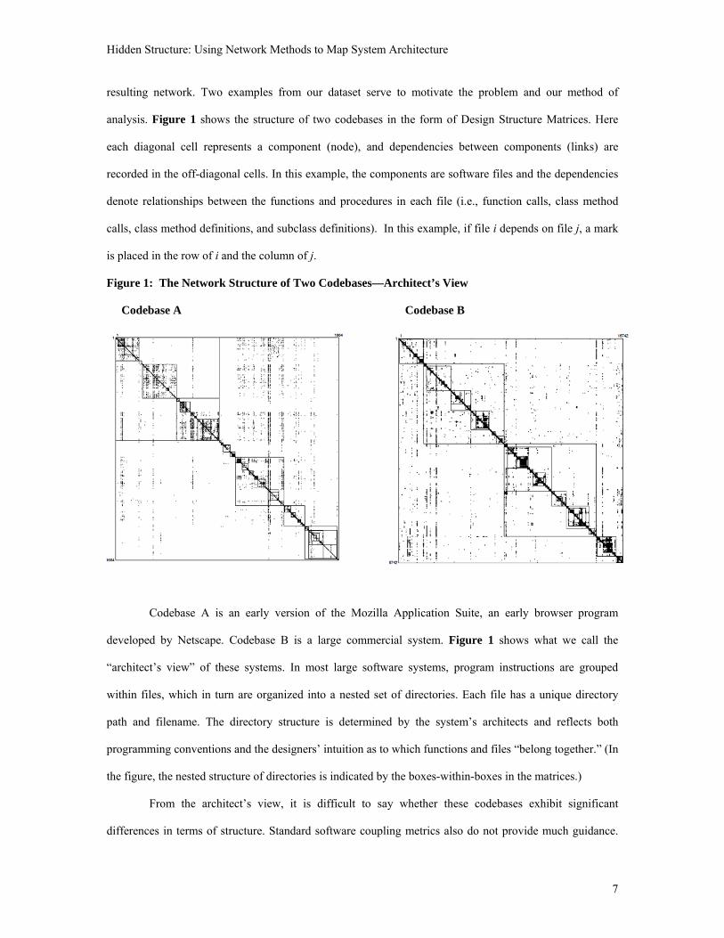
resulting network. Two examples from our dataset serve to motivate the problem and our method of
analysis. Figure 1 shows the structure of two codebases in the form of Design Structure Matrices. Here
each diagonal cell represents a component (node), and dependencies between components (links) are
recorded in the off-diagonal cells. In this example, the components are software files and the dependencies
denote relationships between the functions and procedures in each file (i.e., function calls, class method
calls, class method definitions, and subclass definitions). In this example, if file i depends on file j, a mark
is placed in the row of i and the column of j.
Figure 1: The Network Structure of Two Codebases—Architect’s View
Codebase A Codebase B
Codebase A is an early version of the Mozilla Application Suite, an early browser program
developed by Netscape. Codebase B is a large commercial system. Figure 1 shows what we call the
“architect’s view” of these systems. In most large software systems, program instructions are grouped
within files, which in turn are organized into a nested set of directories. Each file has a unique directory
path and filename. The directory structure is determined by the system’s architects and reflects both
programming conventions and the designers’ intuition as to which functions and files “belong together.” (In
the figure, the nested structure of directories is indicated by the boxes-within-boxes in the matrices.)
From the architect’s view, it is difficult to say whether these codebases exhibit significant
differences in terms of structure. Standard software coupling metrics also do not provide much guidance.
Hidden Structure: Using Network Methods to Map System Architecture
8
For example, according to Chidamber and Kemerer’s (1994) coupling metric, a measure often used in
software engineering, Codebase A has a coupling of 5.39, while Codebase B has a coupling of 4.86. In
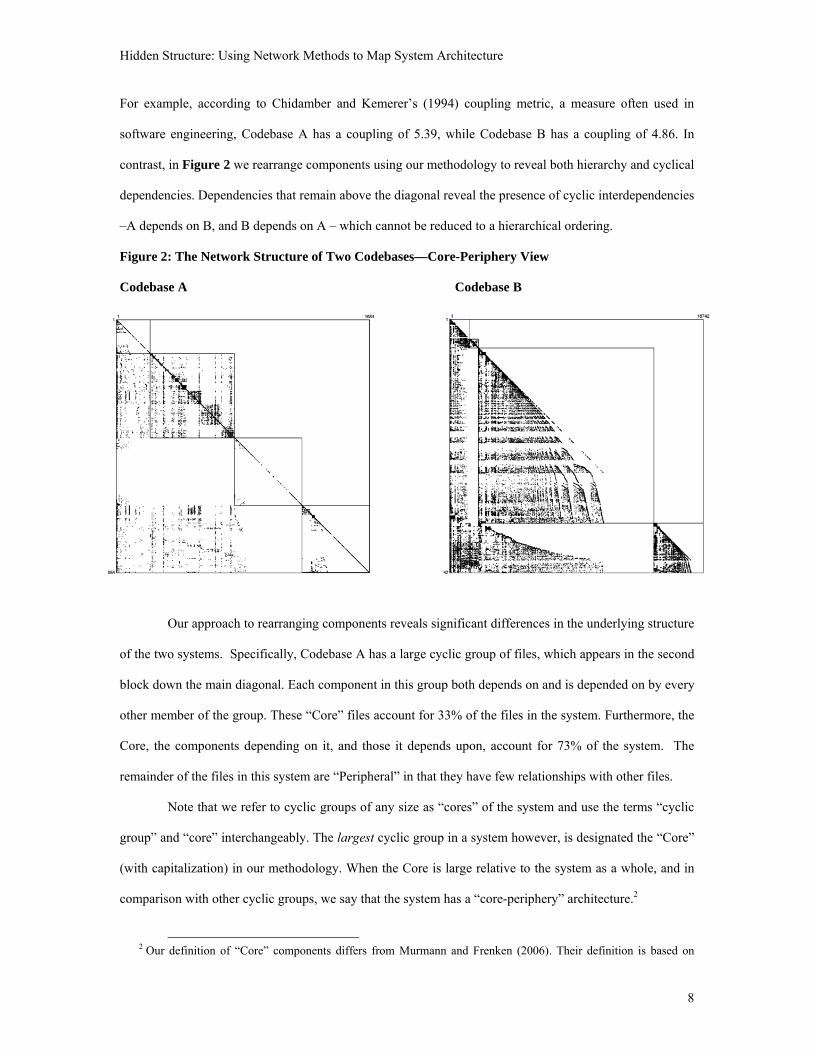
contrast, in Figure 2 we rearrange components using our methodology to reveal both hierarchy and cyclical
dependencies. Dependencies that remain above the diagonal reveal the presence of cyclic interdependencies
–A depends on B, and B depends on A – which cannot be reduced to a hierarchical ordering.
Figure 2: The Network Structure of Two Codebases—Core-Periphery View Codebase A Codebase B
Our approach to rearranging components reveals significant differences in the underlying structure
of the two systems. Specifically, Codebase A has a large cyclic group of files, which appears in the second
block down the main diagonal. Each component in this group both depends on and is depended on by every
other member of the group. These “Core” files account for 33% of the files in the system. Furthermore, the
Core, the components depending on it, and those it depends upon, account for 73% of the system. The
remainder of the files in this system are “Peripheral” in that they have few relationships with other files.
Note that we refer to cyclic groups of any size as “cores” of the system and use the terms “cyclic
group” and “core” interchangeably. The largest cyclic group in a system however, is designated the “Core”
(with capitalization) in our methodology. When the Core is large relative to the system as a whole, and in
comparison with other cyclic groups, we say that the system has a “core-periphery” architecture.2
2 Our definition of “Core” components differs from Murmann and Frenken (2006). Their definition is based on

Hidden Structure: Using Network Methods to Map System Architecture
9
Returning to our example, we note that the largest cyclic group in Codebase B is much smaller in
relation to the system as a whole, accounting for only 3.5% of system files. Almost 70% of the files in this
system—shown in the third block down the main diagonal—lie on pathways that do not depend upon the
Core. Systems such as these display a high level of ordering in the dependencies among components, thus
we call this a “hierarchical” architecture. Critically, the structural relationships revealed by Figure 2 cannot
be inferred from standard measures of coupling nor from DSMs based on the architect’s view alone. In the
subsections below, we present a methodology that makes this “hidden structure” visible and describe
metrics that can be used to compare systems and track changes in system structure over time.
3.1 Overview of Methodology and Rationale
A brief overview of our methodologly is as follows (the technical terms are fully defined in
sections below). First, we identify the direct and indirect dependencies between system components in a
DSM. We then use these measures to identify the cyclic groups (cores) of the system. Based on the size of
the largest cyclic group relative to the system and to other cores, we classify the system architecture as
“core-periphery,” “multi-core,” or “hierarchical.” Next we divide the components into four groups based on
their hierarchical relationship with the largest cyclic group (Core). Finally, we place the four component
groups in order along the main diagonal of a new matrix, and within each group, sort the components to
achieve a lower-diagonalized array. Appendix A provides a step-by-step description of the methodology.
These steps constitute an empirical methodology whose purpose is to reveal both cyclic groups
(cores) and hierarchical relationships among the components of a large system. Different parts of this
methodology, however, are motivated by different concerns. First, our concern with hierarchical orderings
and cyclic groups is motivated by the theories of dominant designs, design cycles, and design cost. Our
classification of architectures arose in response to empirical regularities discovered in our dataset. Finally
our method of ordering component groups in a new DSM stems from a desire to represent hidden
architectural patterns in visual form. Of course, the methodology presented in this paper is not the only way
to analyze the architecture of large technical systems. Nevertheless, in our empirical work across a large
range of systems, we have found it is a powerful way to discover a system’s hidden structure, classify
architectures, and visualize the relationships among a system’s components. Below, we describe this
hierarchical ordering only and does not take account of cyclic groups.
Hidden Structure: Using Network Methods to Map System Architecture
10
methodology in detail.
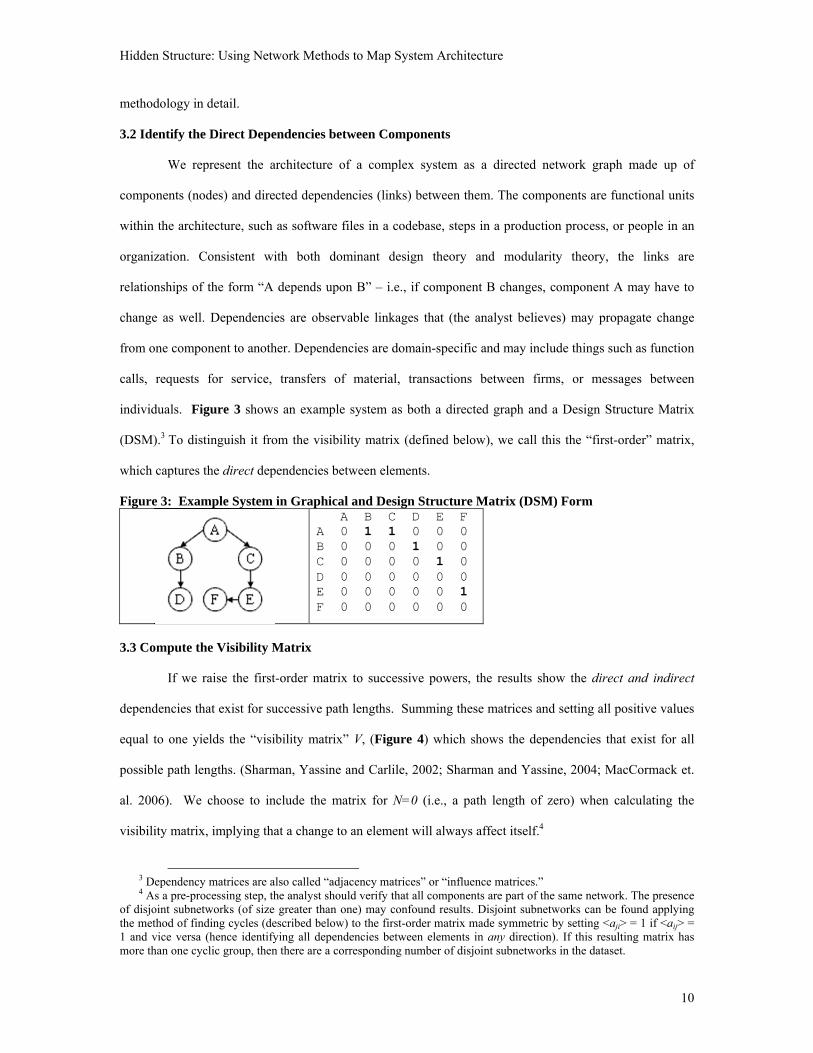
3.2 Identify the Direct Dependencies between Components We represent the architecture of a complex system as a directed network graph made up of
components (nodes) and directed dependencies (links) between them. The components are functional units
within the architecture, such as software files in a codebase, steps in a production process, or people in an
organization. Consistent with both dominant design theory and modularity theory, the links are
relationships of the form “A depends upon B” – i.e., if component B changes, component A may have to
change as well. Dependencies are observable linkages that (the analyst believes) may propagate change
from one component to another. Dependencies are domain-specific and may include things such as function
calls, requests for service, transfers of material, transactions between firms, or messages between
individuals. Figure 3 shows an example system as both a directed graph and a Design Structure Matrix
(DSM).3 To distinguish it from the visibility matrix (defined below), we call this the “first-order” matrix,
which captures the direct dependencies between elements.
Figure 3: Example System in Graphical and Design Structure Matrix (DSM) Form
A B C D E F A 0 1 1 0 0 0 B 0 0 0 1 0 0 C 0 0 0 0 1 0 D 0 0 0 0 0 0 E 0 0 0 0 0 1 F 0 0 0 0 0 0
3.3 Compute the Visibility Matrix
If we raise the first-order matrix to successive powers, the results show the direct and indirect
dependencies that exist for successive path lengths. Summing these matrices and setting all positive values
equal to one yields the “visibility matrix” V, (Figure 4) which shows the dependencies that exist for all
possible path lengths. (Sharman, Yassine and Carlile, 2002; Sharman and Yassine, 2004; MacCormack et.
al. 2006). We choose to include the matrix for N=0 (i.e., a path length of zero) when calculating the
visibility matrix, implying that a change to an element will always affect itself.4
3 Dependency matrices are also called “adjacency matrices” or “influence matrices.” 4 As a pre-processing step, the analyst should verify that all components are part of the same network. The presence
of disjoint subnetworks (of size greater than one) may confound results. Disjoint subnetworks can be found applying the method of finding cycles (described below) to the first-order matrix made symmetric by setting <aji> = 1 if <aij> = 1 and vice versa (hence identifying all dependencies between elements in any direction). If this resulting matrix has more than one cyclic group, then there are a corresponding number of disjoint subnetworks in the dataset.

Hidden Structure: Using Network Methods to Map System Architecture
11
Figure 4: Visibility Matrix for the Example in Figure 3
V = Mn ; n = [0,4] A B C D E F A 1 1 1 1 1 1 B 0 1 0 1 0 0 C 0 0 1 0 1 1 D 0 0 0 1 0 0 E 0 0 0 0 1 1 F 0 0 0 0 0 1
The visibility matrix, V, is identical to the “transitive closure” of the first-order matrix. That is, it
shows all direct and indirect dependencies between components in the system. Transitive closure can be
calculated via matrix multiplication or algorithms such as Warshall’s algorithm (Stein, Drysdale and Bogart,
2011). Algorithms for matrix multiplication and for calculating transitive closure are widely available and
are active areas of mathematical research. Those used in computational programming languages such as
Matlab™ or Mathematica™, are heavily optimized and updated as new and better approaches are
discovered. Our strategy is to take these algorithms as given and build upon them.
3.4 Construct Measures from the Visibility Matrix From the visibility matrix, V, we construct several measures. First, for each component (i) in the
system we define:
VFIi (Visibility Fan-In) is the number of components that directly or indirectly depend on i. This number can be found by summing the entries in the ith column of V.
VFOi (Visibility Fan-out) is the number of components that i directly or indirectly depends on. This number can be found by summing the entries in the ith row of V.
In Figure 4, element A has VFI equal to 1, meaning that no other components depend on it, and
VFO equal to 6, meaning that it depends on all other components (including itself).
In prior work (MacCormack et. al., 2006, 2012), Propagation Cost has been defined as the density
of the visibility matrix, and is used to measure visibility at the system level. Intuitively, Propagation Cost
equals the fraction of the system that could potentially be affected when a change is made to a randomly
selected component. While Propagation Cost is not the focus of this paper, it is an important measure of a
system’s architectural complexity. We include it here for completeness:
Propagation Cost (PC) VFIi
i1
N
N 2
VFOi
i1
N
N 2

Hidden Structure: Using Network Methods to Map System Architecture
12
3.5 Find and Rank the Size of All Cyclic Groups The next step is to find all of the cyclic groups in the system. By definition, each component
within a cyclic group depends directly or indirectly on every other member of the group. Hence:
Proposition 1. Every member of a cyclic group has the same VFI and VFO as every other member. (All proofs are given in Appendix B.) If we sort components using their measures of visibility, the members of cyclic groups will therefore appear
next to each other in the dataset.
Method to Find Cyclic Groups
(1) Sort the components, first by VFI descending, then by VFO ascending. (Other sort orders are
discussed in Appendix C.)
(2) Proceed through the sorted list, comparing the VFIs and VFOs of adjacent components. If the VFI
and VFO for two successive components are the same, then by Proposition 1, they might be
members of the same cyclic group.
(3) For a group of components with the same VFI and VFO inspect the subset of the visibility matrix
that includes the rows and columns of the group in question and no others. If there are no zeros in
the submatrix, then all components are members of the same cyclic group. If there are zeros in
this submatrix, then the group contains two or more separate cyclic groups.
(4) If they exist, identify the separate cyclic groups by (a) selecting any component, i, in the
submatrix; (b) identifying all other components in the submatrix such that <vij> = 1 (equivalently
<vji> = 1). These components will be in the same cyclic group as i. Repeat this procedure until all
the components in the submatrix have been accounted for.5
(5) Count the cyclic groups in the system and the number of components in each. The largest cyclic
group is labeled the “Core” (with capitalization), and is the focus of subsequent analysis.
3.6 Classify the Architecture according to the Size of the Core Theoretically, systems can range from being purely hierarchical (i.e., have no cyclic groups) to
being comprised of any number of cyclic groups of different sizes. Our classification scheme focuses on the
largest cyclic group. It is motivated by a strong empirical regularity in our dataset, which we describe next.
5 We are grateful to Dan Sturtevant for identifying us how to quickly identify separate cyclic groups.

Hidden Structure: Using Network Methods to Map System Architecture
13
Figure 5 presents a scatter plot of visibility measures for the components in Codebase A, with VFI
on the vertical dimension and VFO on the horizontal dimension. The scatter has a “four-square” structure,
indicating that there are four basic groups of components, located in the four quadrants of the graph.
Figure 5: Scatter Plot of Components (Files) for Codebase A (Mozilla)
First, the largest cyclic group appears in the upper right quadrant with VFI (=1009) and VFO
(=768). This group contains 561 interconnected components, and is larger than any other cyclic group in
the system, hence we label it the “Core”. The Core contains 33% of the components in this system and is
16 times larger than the next largest cyclic group. The 448 components that depend on the Core appear in
the lower right quadrant of the scatter plot. We label these “Control” components because they make use of
other components in the system but are not themselves used by others. The 225 components that the Core
depends on appear in the top left quadrant of the graph. We label these “Shared” components. Finally, 455
components appear in the lower left quadrant of the graph. None of these files depends on the Core and the
Core cannot depend on them. We call them “Peripheral” components.
In our empirical work, we observed this “four-square” pattern of VFI and VFO dependencies
frequently. The most salient characteristic of this pattern is the size and centrality of the largest cyclic
group, the Core. In such systems, dependencies are transmitted from Control components, through Core
components, to Shared components. At the same time, there are other components (the Periphery) that
0
200
400
600
800
1000
1200
0 100 200 300 400 500 600 700 800 900 1000
Visibility
Fan
‐in (V
FI)
Visibility Fan‐out (VFO)
Codebase A (Mozilla)
"Core" 561 files, 1 cyclic group
"Shared" 225 files
"Periphery" 450 files
"Control" 448 files
Hidden Structure: Using Network Methods to Map System Architecture
14
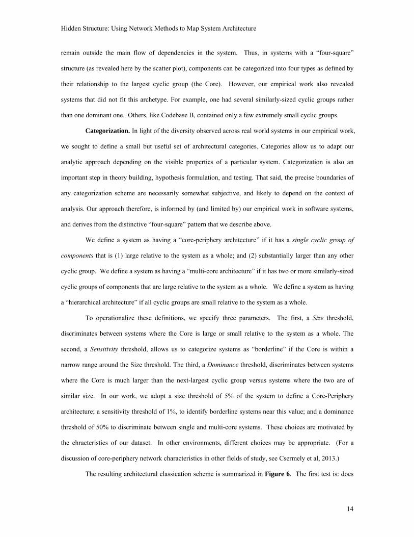
remain outside the main flow of dependencies in the system. Thus, in systems with a “four-square”
structure (as revealed here by the scatter plot), components can be categorized into four types as defined by
their relationship to the largest cyclic group (the Core). However, our empirical work also revealed
systems that did not fit this archetype. For example, one had several similarly-sized cyclic groups rather
than one dominant one. Others, like Codebase B, contained only a few extremely small cyclic groups.
Categorization. In light of the diversity observed across real world systems in our empirical work,
we sought to define a small but useful set of architectural categories. Categories allow us to adapt our
analytic approach depending on the visible properties of a particular system. Categorization is also an
important step in theory building, hypothesis formulation, and testing. That said, the precise boundaries of
any categorization scheme are necessarily somewhat subjective, and likely to depend on the context of
analysis. Our approach therefore, is informed by (and limited by) our empirical work in software systems,
and derives from the distinctive “four-square” pattern that we describe above.
We define a system as having a “core-periphery architecture” if it has a single cyclic group of
components that is (1) large relative to the system as a whole; and (2) substantially larger than any other
cyclic group. We define a system as having a “multi-core architecture” if it has two or more similarly-sized
cyclic groups of components that are large relative to the system as a whole. We define a system as having
a “hierarchical architecture” if all cyclic groups are small relative to the system as a whole.
To operationalize these definitions, we specify three parameters. The first, a Size threshold,
discriminates between systems where the Core is large or small relative to the system as a whole. The
second, a Sensitivity threshold, allows us to categorize systems as “borderline” if the Core is within a
narrow range around the Size threshold. The third, a Dominance threshold, discriminates between systems
where the Core is much larger than the next-largest cyclic group versus systems where the two are of
similar size. In our work, we adopt a size threshold of 5% of the system to define a Core-Periphery
architecture; a sensitivity threshold of 1%, to identify borderline systems near this value; and a dominance
threshold of 50% to discriminate between single and multi-core systems. These choices are motivated by
the chracteristics of our dataset. In other environments, different choices may be appropriate. (For a
discussion of core-periphery network characteristics in other fields of study, see Csermely et al, 2013.)
The resulting architectural classication scheme is summarized in Figure 6. The first test is: does
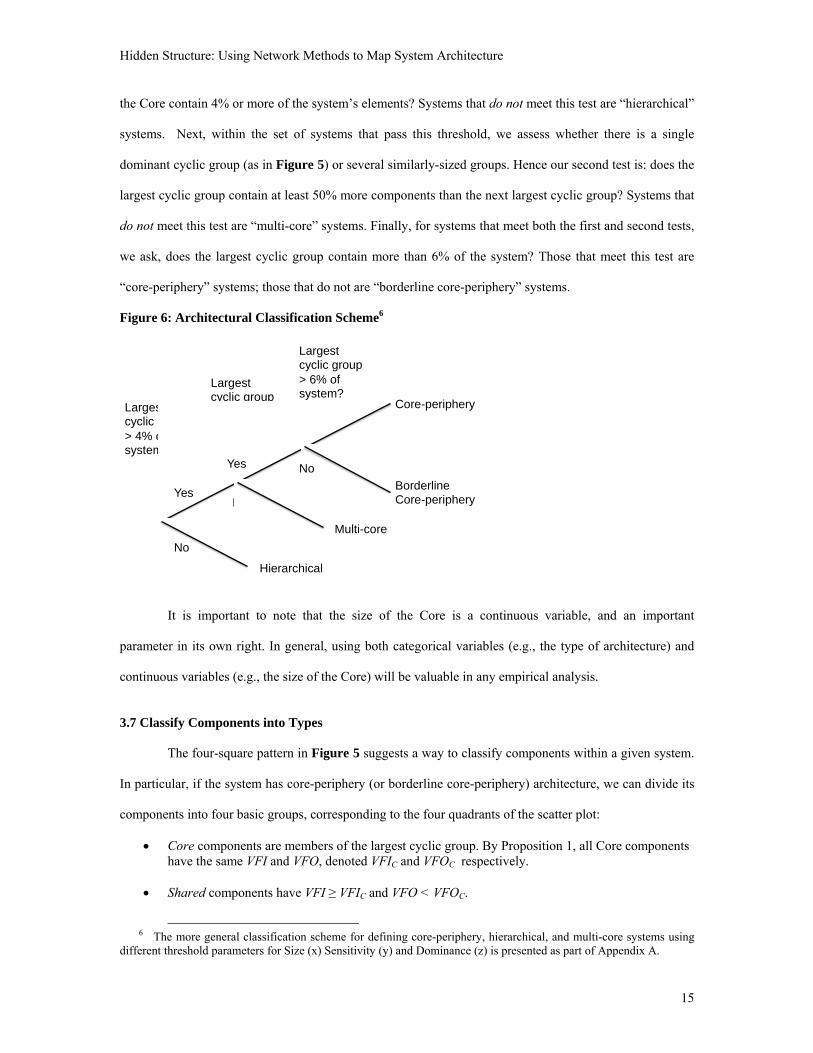
Hidden Structure: Using Network Methods to Map System Architecture
15
the Core contain 4% or more of the system’s elements? Systems that do not meet this test are “hierarchical”
systems. Next, within the set of systems that pass this threshold, we assess whether there is a single
dominant cyclic group (as in Figure 5) or several similarly-sized groups. Hence our second test is: does the
largest cyclic group contain at least 50% more components than the next largest cyclic group? Systems that
do not meet this test are “multi-core” systems. Finally, for systems that meet both the first and second tests,
we ask, does the largest cyclic group contain more than 6% of the system? Those that meet this test are
“core-periphery” systems; those that do not are “borderline core-periphery” systems.
Figure 6: Architectural Classification Scheme6
It is important to note that the size of the Core is a continuous variable, and an important
parameter in its own right. In general, using both categorical variables (e.g., the type of architecture) and
continuous variables (e.g., the size of the Core) will be valuable in any empirical analysis.
3.7 Classify Components into Types
The four-square pattern in Figure 5 suggests a way to classify components within a given system.
In particular, if the system has core-periphery (or borderline core-periphery) architecture, we can divide its
components into four basic groups, corresponding to the four quadrants of the scatter plot:
Core components are members of the largest cyclic group. By Proposition 1, all Core components have the same VFI and VFO, denoted VFIC and VFOC respectively.
Shared components have VFI ≥ VFIC and VFO < VFOC.
6 The more general classification scheme for defining core-periphery, hierarchical, and multi-core systems using
different threshold parameters for Size (x) Sensitivity (y) and Dominance (z) is presented as part of Appendix A.
Yes
Largest cyclic group > 4% of system?
Largest cyclic group > 1.5x next largest?
Yes
No
Yes
No
Core-periphery
Multi-core
Hierarchical
Largest cyclic group > 6% of system?
Borderline Core-periphery
No

Hidden Structure: Using Network Methods to Map System Architecture
16
Peripheral components have VFI < VFIC and VFO < VFOC.
Control components have VFI < VFIC and VFO ≥ VFOC.
In hierarchical or multi-core architectures, this partitioning can be problematic. First, components
may not naturally fall into four distinct categories (e.g., there may be no cyclic groups). Second, in multi-
core systems, the classification of components may not be stable over time: if one cyclic group grows
larger than another, the identity of the “Core” may change, even if the overall pattern of dependencies
changes little. Third, in hierarchical systems, this partitioning may result in unbalanced numbers of
components in each category, creating challenges for statistical analysis.
To address these issues, we define an alternative way to classify components, based on the median
values of VFI and VFO. When applied to hierarchical and/or multi-core systems, the median partition
yields groupings that are more equal in size and more stable over time (assuming dependency patterns do
not change significantly).7 In a partition based on medians, the high-VFI and high-VFO components will
not, in general, be members of the same cyclic group, hence we call these components “Central” (instead of
“Core”). Similarly, the remaining categories are identified as Shared-M, Control-M and Periphery-M.
3.8 Visualize the Architecture
The final step in our methodology allows us to reorder the components to construct a new DSM
that reveals the “hidden structure” of the system:
(1) Place components in the order Shared, Core (or Central), Periphery, Control down the main diagonal of the DSM; and then
(2) Sort within each group by VFI descending, then VFO ascending. This methodology results in a reordered DSM with the following properties:
Cyclic groups are clustered around the main diagonal.
There are no dependencies across groups above the main diagonal.
There are no dependencies between the Core (or Central) group and the Periphery above or below the main diagonal.
Except for cyclic groups, each block is lower diagonalized (i.e., has no dependencies above the
diagonal).
7 It may be necessary to exclude “singletons” (i.e., components with VFI = VFO = 1), to get balanced groups when using the median partition. As noted above, these components are, strictly speaking, not part of the same network.

Hidden Structure: Using Network Methods to Map System Architecture
17
The first property is a consequence of Proposition 1. The other properties are proved in Appendix B.
If the largest cyclic group is the basis of the partition, we call this the “core-periphery view” of the
system. If medians are the basis of the partition, we call it the “median view.” Figure 7 shows both views
for Codebase B. In general, these different views are complementary ways of visualizing the flow of
dependencies in a large technical system. The core-periphery view is more informative as the largest cyclic
group increases in size relative to the system as whole and other cyclic groups. However, we have found
that, especially in borderline cases, both views generate helpful information for analysis.
Figure 7: Core-Periphery and Median Views of Codebase B (a Hierarchical System)
Core-Periphery View Median View
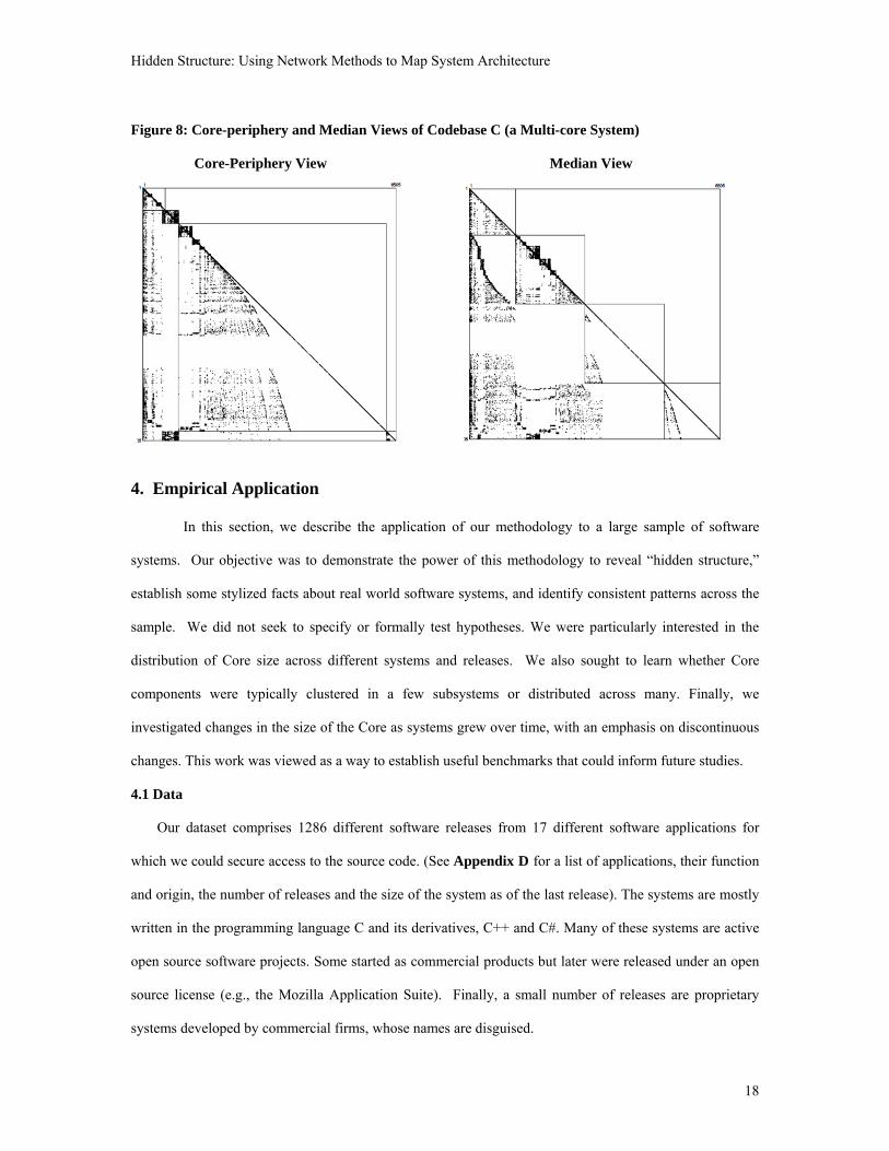
Figure 8 shows the core-periphery and median views for Codebase C, a multi-core system.
Codebase C is a version of Open Office, an open source suite of applications that includes a word processor,
a spreadsheet program, and a presentation manager. The multiple cores in this system correspond to the
different applications. As anticipated above, the core-periphery view results in unbalanced groupings: 82%
of the system including the second and third largest cyclic groups are placed in the periphery. The median
partition, by contrast, results in more balanced groupings and places all signficant cyclic groups in the
“Central” category. It also reveals interesting subsidiary structures: for example, the three largest cyclic
groups appear to be independent (which can be easily verified from the reordered DSM).
Shared-M
Central
Periphery-M
Control-M
Shared Core
Periphery
Control
Hidden Structure: Using Network Methods to Map System Architecture
18
Figure 8: Core-periphery and Median Views of Codebase C (a Multi-core System)
Core-Periphery View Median View
4. Empirical Application
In this section, we describe the application of our methodology to a large sample of software
systems. Our objective was to demonstrate the power of this methodology to reveal “hidden structure,”
establish some stylized facts about real world software systems, and identify consistent patterns across the
sample. We did not seek to specify or formally test hypotheses. We were particularly interested in the
distribution of Core size across different systems and releases. We also sought to learn whether Core
components were typically clustered in a few subsystems or distributed across many. Finally, we
investigated changes in the size of the Core as systems grew over time, with an emphasis on discontinuous
changes. This work was viewed as a way to establish useful benchmarks that could inform future studies.
4.1 Data
Our dataset comprises 1286 different software releases from 17 different software applications for
which we could secure access to the source code. (See Appendix D for a list of applications, their function
and origin, the number of releases and the size of the system as of the last release). The systems are mostly
written in the programming language C and its derivatives, C++ and C#. Many of these systems are active
open source software projects. Some started as commercial products but later were released under an open
source license (e.g., the Mozilla Application Suite). Finally, a small number of releases are proprietary
systems developed by commercial firms, whose names are disguised.
Hidden Structure: Using Network Methods to Map System Architecture
19
We focused on large software systems that at some point in their history had many users. Hence we do
not include in our sample open source projects from repositories such as SourceForge, which are typically
very small systems. Although some of our systems (e.g., Linux) start small, all had more than three
hundred source files as of the last release in our dataset. That said, our sample is not random nor
representative of the industry; hence we do not claim our results are general. As indicated above, this
exploratory research provides a starting point for subsequent empirical investigation and hypothesis testing.
We obtained the source code for each release in the sample and processed it to identify dependencies
between source files, specifically function calls, class method calls, class method definitions, and subclass
definitions.8 We used this data to calculate VFI and VFO for each file and the Propagation Cost for each
release. Applying our methodology, we identified the Core for each release, classified architectures as
core-periphery, borderline, hierarchical, or multi-core, and classified all components into groups.
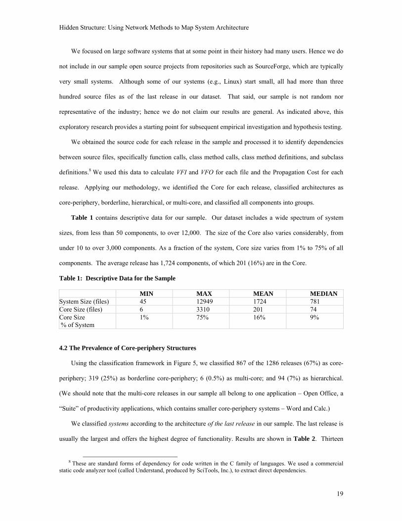
Table 1 contains descriptive data for our sample. Our dataset includes a wide spectrum of system
sizes, from less than 50 components, to over 12,000. The size of the Core also varies considerably, from
under 10 to over 3,000 components. As a fraction of the system, Core size varies from 1% to 75% of all
components. The average release has 1,724 components, of which 201 (16%) are in the Core.
Table 1: Descriptive Data for the Sample
MIN MAX MEAN MEDIAN System Size (files) 45 12949 1724 781 Core Size (files) 6 3310 201 74 Core Size % of System
1% 75% 16% 9%
4.2 The Prevalence of Core-periphery Structures
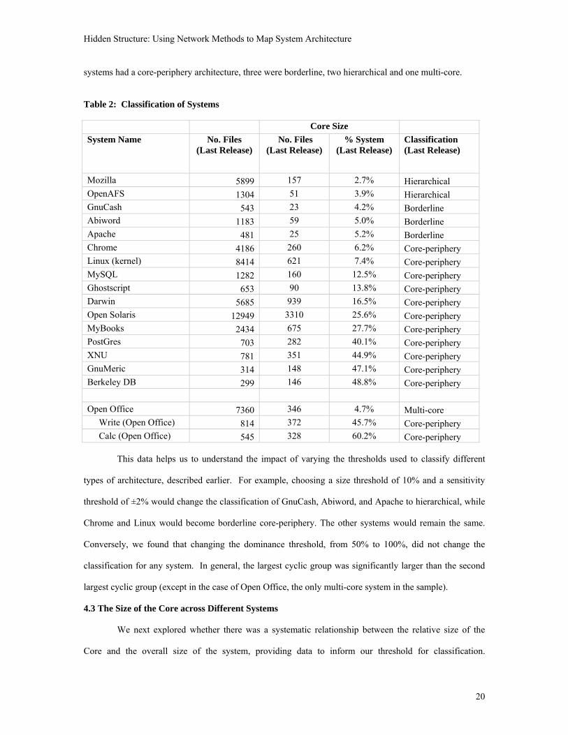
Using the classification framework in Figure 5, we classified 867 of the 1286 releases (67%) as core-
periphery; 319 (25%) as borderline core-periphery; 6 (0.5%) as multi-core; and 94 (7%) as hierarchical.
(We should note that the multi-core releases in our sample all belong to one application – Open Office, a
“Suite” of productivity applications, which contains smaller core-periphery systems – Word and Calc.)
We classified systems according to the architecture of the last release in our sample. The last release is
usually the largest and offers the highest degree of functionality. Results are shown in Table 2. Thirteen
8 These are standard forms of dependency for code written in the C family of languages. We used a commercial
static code analyzer tool (called Understand, produced by SciTools, Inc.), to extract direct dependencies.
Hidden Structure: Using Network Methods to Map System Architecture
20
systems had a core-periphery architecture, three were borderline, two hierarchical and one multi-core.
Table 2: Classification of Systems
Core Size
System Name No. Files (Last Release)
No. Files (Last Release)
% System (Last Release)
Classification (Last Release)
Mozilla 5899 157 2.7% Hierarchical OpenAFS 1304 51 3.9% Hierarchical GnuCash 543 23 4.2% Borderline Abiword 1183 59 5.0% Borderline Apache 481 25 5.2% Borderline Chrome 4186 260 6.2% Core-periphery Linux (kernel) 8414 621 7.4% Core-periphery MySQL 1282 160 12.5% Core-periphery Ghostscript 653 90 13.8% Core-periphery Darwin 5685 939 16.5% Core-periphery Open Solaris 12949 3310 25.6% Core-periphery MyBooks 2434 675 27.7% Core-periphery PostGres 703 282 40.1% Core-periphery XNU 781 351 44.9% Core-periphery GnuMeric 314 148 47.1% Core-periphery Berkeley DB 299 146 48.8% Core-periphery Open Office 7360 346 4.7% Multi-core Write (Open Office) 814 372 45.7% Core-periphery Calc (Open Office) 545 328 60.2% Core-periphery
This data helps us to understand the impact of varying the thresholds used to classify different
types of architecture, described earlier. For example, choosing a size threshold of 10% and a sensitivity
threshold of ±2% would change the classification of GnuCash, Abiword, and Apache to hierarchical, while
Chrome and Linux would become borderline core-periphery. The other systems would remain the same.
Conversely, we found that changing the dominance threshold, from 50% to 100%, did not change the
classification for any system. In general, the largest cyclic group was significantly larger than the second
largest cyclic group (except in the case of Open Office, the only multi-core system in the sample).
4.3 The Size of the Core across Different Systems
We next explored whether there was a systematic relationship between the relative size of the
Core and the overall size of the system, providing data to inform our threshold for classification.

Hidden Structure: Using Network Methods to Map System Architecture
21
Accordingly, Figure 9 plots Core size (as a % of the system) against system size for all releases in our
dataset. The graph differentiates between systems that began as open source projects (denoted as light
circles), versus those that originated as commercial products developed by firms (denoted as dark triangles).
Figure 9: The Size of the Core (Largest Cyclic Group) versus Total System Size
For very small systems, the relative size of the Core varies substantially, from less than 5% to a maximum
of 75% of the system. For larger systems however, the Core declines as a percent of the system. Indeed
there appears to be a negative exponential relationship between Core size and system size. Intuitively, this
pattern makes sense. In small systems, a relatively large Core is still small in absolute terms, hence
architects and developers can still comprehend its internal structure easily. In larger systems however, even
a moderately sized Core creates cognitive and coordination challenges, given that architects must
understand and communicate with each other about many possible direct and indirect interdependencies.
Larger systems thus benefit by having relatively smaller Cores (as a % of the whole).
The graph reveals that, with the exception of Open Solaris, as system size increases, Core sizes
appear to cluster tightly in a band centered around 5%: for a system of 6000 files, this corresponds to a
cyclic group of 300 files, which is large in absolute terms. This data influenced the decision as to the
0.00%
10.00%
20.00%
30.00%
40.00%
50.00%
60.00%
70.00%
80.00%
0 2000 4000 6000 8000 10000 12000 14000
Size
of Largets
Cyclic
Group
(% of S
ystem
Size)
System Size (No. Files)
Open Systems Closed Systems
Open Solaris
Core‐Periphery Threshold (x = 5%)
Hidden Structure: Using Network Methods to Map System Architecture
22
appropriate size threshold (5%) and sensitivity threshold (1%) for our architectural classification scheme.
In future empirical work, we expect these thresholds may be refined, updated for different contexts, and
potentially, new tests added that expand the scheme, to create new architectural categories.9
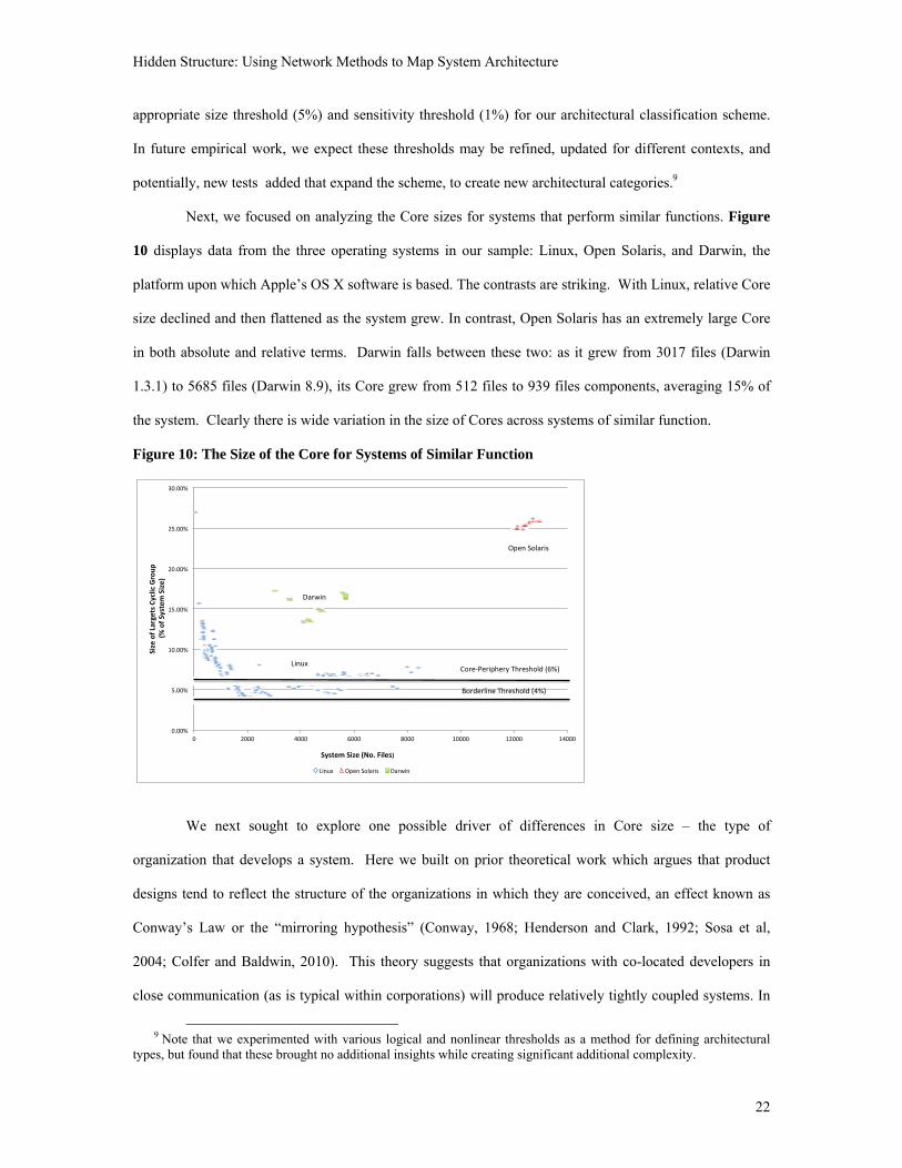
Next, we focused on analyzing the Core sizes for systems that perform similar functions. Figure
10 displays data from the three operating systems in our sample: Linux, Open Solaris, and Darwin, the
platform upon which Apple’s OS X software is based. The contrasts are striking. With Linux, relative Core
size declined and then flattened as the system grew. In contrast, Open Solaris has an extremely large Core
in both absolute and relative terms. Darwin falls between these two: as it grew from 3017 files (Darwin
1.3.1) to 5685 files (Darwin 8.9), its Core grew from 512 files to 939 files components, averaging 15% of
the system. Clearly there is wide variation in the size of Cores across systems of similar function.
Figure 10: The Size of the Core for Systems of Similar Function
We next sought to explore one possible driver of differences in Core size – the type of
organization that develops a system. Here we built on prior theoretical work which argues that product
designs tend to reflect the structure of the organizations in which they are conceived, an effect known as
Conway’s Law or the “mirroring hypothesis” (Conway, 1968; Henderson and Clark, 1992; Sosa et al,
2004; Colfer and Baldwin, 2010). This theory suggests that organizations with co-located developers in
close communication (as is typical within corporations) will produce relatively tightly coupled systems. In
9 Note that we experimented with various logical and nonlinear thresholds as a method for defining architectural
types, but found that these brought no additional insights while creating significant additional complexity.
0.00%
5.00%
10.00%
15.00%
20.00%
25.00%
30.00%
0 2000 4000 6000 8000 10000 12000 14000
Size
of Largets
Cyclic
Group
(%
of S
ystem
Size)
System Size (No. Files)
Linux Open Solaris Darwin
Open Solaris
Core‐Periphery Threshold (6%)
Darwin
Linux
Borderline Threshold (4%)

Hidden Structure: Using Network Methods to Map System Architecture
23
contrast, organizations with geographically distributed developers not in close communication (as is typical
of open source projects) will produce relatively loosely coupled systems. A relatively large (or small) Core
is in turn evidence of tighter (or looser) coupling among the components in a system.
To conduct this analysis, we compared systems with similar functions that emerged from different
types of organizations, specifically, open source versus commercial firms. We used a matched-pair design,
comparing the size of the Core between systems of similar size and function. Our sample was based on a
prior study that explored differences in the propagation cost between open source and commercial systems
(See MacCormack et al, 2012 for details on how the matched pairs were selected.)
Table 3 shows the size of the Core (relative to system size) for our five matched pairs. In every
case, the systems that originated as open source projects have smaller Cores than systems that originated as
commercial products inside firms. In one case (financial management software), the open source system
has a hierarchical architecture, while the commercial system of comparable size has a Core that accounts
for 70% of the system. Although many other factors influence the design of system architectures, this
comparison, as well as the prior study, provides strong evidence that differences in architecture and
particularly in Core size are driven, in part, by differences in the developing organization.
Table 3: The Size of the Core for a Sample of Matched-Pair Products Application Category Open Source Product Closed (Commercial)
Product
System Size Core Size System Size Core Size
Financial Mgmt 466 3.4% 471 69.60%
Word Processor 841 6.10% 790 46.10%
Spreadsheet 450 25.80% 532 57.30%
Operating System 1032 6.30% 994 28.00%
Database 465 7.70% 344 48.80%
4.4 Detecting the Existence and Location of Core Components in a System
It is natural to ask whether the presence of a dominant cyclic group, (hence a core-periphery
architecture) can be detected from the summary statistics for a system (e.g., number of files, directories or
lines of code, average number of dependencies per file) or from inspection of the first-order matrix. To
explore this question, we compared systems that possessed a core-periphery architecture with those that did
not, focusing on differences in both the quantitative data and the visual plots of DSMs using the architect’s
Hidden Structure: Using Network Methods to Map System Architecture
24
view (i.e. sorting files by directory as in Figure 1). We found no variable that could reliably predict
whether a system possessed a core-periphery structure, and no consistent pattern of direct dependencies in
the architectural view of a DSM that would signal the presence of dominant cyclic group. Thus detecting
the presence of a core-periphery architecture cannot be achieved solely by examining the direct
dependencies for a system. Rather, this analysis depends critically on an assessment of the indirect paths
by which dependencies propagate.
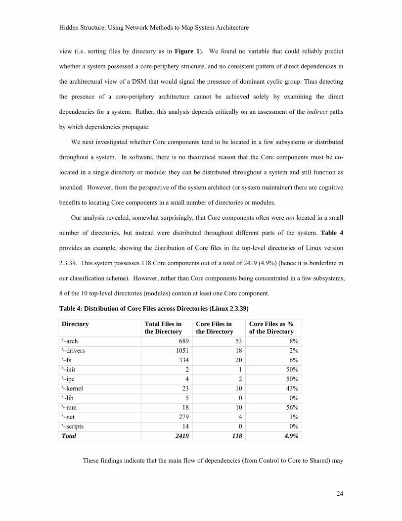
We next investigated whether Core components tend to be located in a few subsystems or distributed
throughout a system. In software, there is no theoretical reason that the Core components must be co-
located in a single directory or module: they can be distributed throughout a system and still function as
intended. However, from the perspective of the system architect (or system maintainer) there are cognitive
benefits to locating Core components in a small number of directories or modules.
Our analysis revealed, somewhat surprisingly, that Core components often were not located in a small
number of directories, but instead were distributed throughout different parts of the system. Table 4
provides an example, showing the distribution of Core files in the top-level directories of Linux version
2.3.39. This system possesses 118 Core components out of a total of 2419 (4.9%) (hence it is borderline in
our classification scheme). However, rather than Core components being concentrated in a few subsystems,
8 of the 10 top-level directories (modules) contain at least one Core component.
Table 4: Distribution of Core Files across Directories (Linux 2.3.39) Directory Total Files in
the Directory Core Files in the Directory
Core Files as % of the Directory
'~arch 689 53 8%
'~drivers 1051 18 2%
'~fs 334 20 6%
'~init 2 1 50%
'~ipc 4 2 50%
'~kernel 23 10 43%
'~lib 5 0 0%
'~mm 18 10 56%
'~net 279 4 1%
'~scripts 14 0 0%
Total 2419 118 4.9%
These findings indicate that the main flow of dependencies (from Control to Core to Shared) may

Hidden Structure: Using Network Methods to Map System Architecture
25
not be immediately apparent from an inspection of the parts of a system that are most salient to the architect.
Simply reviewing the directory structure will generally not be sufficient to reveal where Core components
are located. As a consequence, changes to a Core component may propagate to other Core components in
seemingly remote parts of the system, making it difficult to predict performance. This issue is especially
pertinent when a legacy system must be maintained or adapted with limited documentation. Only through a
detailed analysis of chains of both direct and indirect dependencies can the “hidden structure” of the system
be made visible, affirming the value of our methodology.
4.5 The Evolution of System Structure
In the final application of our methodology, we analyzed how the Cores of various systems
evolved over time (i.e., across successive versions of each application). We found no simple or consistent
pattern to this evolution. In three of the applications, relative Core size declined consistently; in eight
applications, relative Core size remained flat; and for two applications it increased.10 The four remaining
systems however, (Apache, Gnucash, Linux and Mozilla) exhibited discontinuous breaks in Core size as
shown in Figure 11. Hence we further investigated these systems to understand their dynamics.
Figure 11: Systems Exhibiting Discontinuous Breaks in Core Size
A. Apache (released versions only) B. Gnucash
10 In one case (Chrome), we had only one release, hence insufficient data for this analysis.
0%
2%
4%
6%
8%
10%
12%
14%
16%
1 11 21 31 41
Largest
Cyclic
Group
as %
of System
Size
Release Sequence
Apache 2.0.28 – 2.0.52
Apache 1.3.0 ‐ 2.0a9
0%
5%
10%
15%
20%
25%
30%
35%
40%
1 11 21 31 41 51 61 71 81 91 101 111
Largest
Cyclic
Group
as a
% of System
SIze
Release Sequence
gnucash 1.7.1 ‐ 2.2.8
gnucash 1.1.11 – 1.6.8

Hidden Structure: Using Network Methods to Map System Architecture
26
C. Linux (stable releases only) D. Mozilla
The cases of Apache and Gnucash are straightforward. Apache began with a core-periphery
architecture, with a Core in the range of 12% to 14% of system size. A significant redesign of the system
took place between version 2.0.a9 and 2.0.28. In version 2.0.28, the Core dropped to 4% of the system, and
then rose to around 5%. (A borderline system in our classification scheme.) The case of Gnucash is even
more dramatic. Early on, the Core grew significantly from 13 to 70 files or approximately 30% of the
system. With release 1.7.1, however, system size almost doubled (232 to 449 files), but the Core dropped
from 70 to 16 files (3.6% of the system). In later releases, the Core has consistently accounted for 4-5% of
the system, making this system borderline under our classification scheme. Note that both Apache and
Gnucash are relatively small systems in this sample.11 In their size range (below 500 files), Core size
relative to system size varies considerably (see Figure 9). In such systems, Core interdependencies can be
directly inspected and understood by developers, thus architectural changes aimed at reducing the Core
may have low priority.
In contrast, Linux and Mozilla are large systems, which have grown significantly over time. In the
case of Linux, discontinuous changes in the size of the Core have coincided with major releases. 12 Figure
11 C shows that Linux started out as a core-periphery system with the Core initially accounting for just
over 10% of the system. This figure dropped to around 8% for Linux 2.0 and to just over 4% with Linux
11 The last releases in our dataset contained 481 files and 543 files respectively. 12 During the period of our sample, the Linux kernel used an “even-odd” version numbering scheme. Even numbers
in the second place of the release number (e.g., 2.4.19) denoted “stable” releases that were appropriate for wide deployment; odd numbers (e.g., 2.5.19) denoted “development” releases that were the focus of ongoing experimentation. Work on the even and odd numbered releases would go on simultaneously, hence release numbers are in temporal sequence only within two sets. http://www.linfo.org/kernel_version_numbering.html. The even-odd numbering practice was discontinued with the release of version 2.6.0.
0.00%
2.00%
4.00%
6.00%
8.00%
10.00%
12.00%
1 11 21 31 41 51 61 71 81 91 101 111 121 131
Largest
Cyclic
Group
as a %
of System
Size
Release Sequence
Linux 1.2
Linux 2.0
Linux 2.2
Linux 2.4
Linux 2.6
0.00%
5.00%
10.00%
15.00%
20.00%
25.00%
30.00%
35.00%
1 2 3 4 5 6 7 8 9 10 11 12 13 14 15 16 17 18 19 20 21 22 23 24 25 26 27 28 29 30 31 32 33 34 35
Largest
Cyclic Group
as a
% of S
ystem
Size
Release Sequence
M 00 3/31/98 – M 00 10/8/98
M 00 12/11/98 – M12
M 13 – MMX 1.5

Hidden Structure: Using Network Methods to Map System Architecture
27
2.2. However, there were small discontinuous jumps in Core size associated with the release of Linux 2.4
and 2.6. Most releases of Linux 2.4 were borderline, while Linux 2.6 wavered around the 6% threshold.
The Mozilla Application Suite exhibited two discontinuous changes in Core size, although the trend is
consistently downward. (See Figure 11 D.) The first discontinuity occurred in December 1998: the Core
dropped from 680 files (29% of the system) to 223 files (15%). (System size also dropped but not as much.)
Subsequently, the system grew significantly (from 1508 to 3405 files) while the Core grew only slightly
(from 223 to 269 files or 7.9% of the system). We know from prior work that the change in Mozilla’s
design in December 1998 was the result of a purposeful redesign effort, which had the explicit objective of
making the codebase more modular, hence easier for contributors to work within (MacCormack et al, 2006).
As Table 5 shows, achieving this goal led to substantially smaller Core and Shared groups and larger
Periphery and Control groups. (Note that we do not know the reason behind the second discontinuous
change in the architecture of this codebase.)
Table 5: Percent of Components in Each Category before and after the 1998 Mozilla Redesign Type of Component
% before Redesign (4/8/98 Release)
% after Redesign (12/11/98 Release)
Shared 13% 3%
Core 33% 15%
Periphery 27% 36%
Control 27% 46%
Total 100% 100%
To conclude, we found no single pattern to characterize the way the Core of a system evolves over
time. Changes in relative Core size are often continuous (i.e. display no sharp discontinuities), but the Core
may increase, stay the same or decrease in relation to the system as a whole. Thus, for the majority of
applications in our sample, the Core did not seem to be a focus of major redesign efforts. In a few cases,
however, we observe discontinuous changes that seem to be the result of purposeful intervention. The most
dramatic of these resulted in large reductions in the relative size of the Core. Furthermore, in one case
(Mozilla, December 1998), we know from interviews with the architects involved that the purpose of the
redesign was to reduce system complexity. These findings are consistent with the conjecture (from design

Hidden Structure: Using Network Methods to Map System Architecture
28
theory) that cyclical dependencies are problematic because they increase cognitive complexity and the
number of iterations needed to arrive at an acceptable design. However, our parallel observation, that Core
files are dispersed throughout a system’s modules, means that it may be hard to identify the components in
the system that give rise to these problematic cyclical dependencies. A valuable contribution of our
methodology is that it identifies the Core and its members, making this hidden structure more visible.
5. Discussion
In this paper, we describe a robust and reliable methodology to detect the core components in a
complex system, to establish whether these systems possess a core-periphery structure, and to measure
important elements of these structures. Our methodology, which is based upon network graphs, addresses
important limitations of prior analysis methods. In particular, it focuses on directed graphs, disentangling
differences in structure that stem from dependencies that flow in different directions; it captures all of the
direct and indirect dependencies among the components in a system, rather than capturing purely the direct
connections; and it provides a heuristic for rearranging the elements in a system, in a way that helps to
visualize the system architecture and reveals its “hidden structure” (in contrast to other network methods,
which tend to yield visual representations that are hard to comprehend). We apply this methodology to a
large sample of software applications. As a result, we establish some stylized facts about the structure of
real-world systems, to serve as a point of departure for future empirical investigations.
We show that the majority of systems in our sample contain a single cyclic group (the Core) that is
large relative to the system as a whole, and in comparison to the second-largest cyclic group. Other systems
have only a few, small cyclic groups, or (in one case) several cyclic groups of comparable size. The large
variations we observe with respect to the detailed characteristics of these systems however, implies that a
considerable amount of managerial discretion exists when choosing the “best” architecture for a system. .
In particular, there are major differences in the number of Core components across a range of systems of
similar size and function, indicating that the differences in design are not driven solely by system
requirements. Specifically, we find evidence that variations in system structure can be explained, in part, by
the different models of development used to build systems. That is, product structures “mirror” the
structure of their parent organizations (Henderson and Clark, 1990, Sosa et al, 2004; Colfer and Baldwin,

Hidden Structure: Using Network Methods to Map System Architecture
29
2010). This result is consistent with work that argues designs (including dominant designs) are not
necessarily optimal technical solutions to customer requirements, but rather are driven more by social and
political processes operating within firms and industries (Noble, 1984; David, 1985; Tushman and
Rosenkopf, 1992; Tushman and Murmann, 1998; Garud, Jain and Kumaraswamy, 2002).
Our findings highlight in particular, the difficulties facing a system architect. In particular, we find no
discernible pattern of direct dependencies that reliably predicts whether a system has a single, dominant
Core, or if it does, how large it is. This problem is compounded by the fact that in many systems, the Core
components are not located in a small number of subsystems but are distributed throughout the system. The
system architect therefore has to identify where to focus attention; it is not simply a matter of concentrating
on subsystems that appear to contain most of the Core components. Important relationships may exist
between these components and others within subsystems that, on the surface, appear relatively insignificant.
This highlights the need to understand patterns of coupling at the component level, and not to assume that
all of the key relationships in a complex system are located in a few key subsystems or modules.
These issues are especially pertinent in software, given that legacy code is rarely re-written, but instead
forms a platform upon which new versions are built. With such an approach, today’s developers bear the
consequences of design decisions made long ago – obligations increasingly referred to as a system’s
“technical debt.” Unfortunately, the first designers of a system often have different objectives from those
that follow, especially if the system is successful and therefore long lasting. While early designers may
place a premium on speed and performance, later designers may value reliability and maintainability.
Rarely can all these objectives be met by the same design. A different problem stems from the fact that the
early designers of a system may no longer be available when important design choices need revisiting. This
difficulty is compounded by the fact that software designers rarely document their design choices well,
often requiring the structure to be recovered by inspection of the source code (as we do here).
Several limitations of our study must be considered in assessing its generalizability. First, our
empirical work was conducted in the software industry on codebases written for the most part in C and
related languages. Software presents a unique context given that software systems exist purely as
information, and thus are subject to different limitations than physical artifacts. Whether similar results are
found in other settings is an important empirical question (Csermely et al, 2013). However, Luo et al

Hidden Structure: Using Network Methods to Map System Architecture
30
(2012) demonstrate that a core-periphery structure existed in the supply chain network of the Japanese
electronics industry in the mid-1990s. And a recent study by Lagerstrom et al (2014) finds a core-periphery
structure in the enterprise architecture of a large financial services organization. Thus, the evidence is
accumulating that this type of structure is pervasive across different domains, industries and technologies.
Second, we analyzed a non-random sample of systems for which we had access to the source code.
Although we limited our enquiry to successful systems with thousands of user deployments, we cannot be
sure that the results are representative of the industry as a whole. Also, our categorical results are sensitive
to the thresholds selected as breakpoints in our classification scheme. As noted, these thresholds are
necessarily somewhat subjective and may vary by context. Hence the classification of architectures
remains an open avenue for future empirical work, which we expect will prove fuitful.
Our work opens up a number of other avenues for future study. Specifically, prior work suggests that
exogenous technological “shocks” in an industry can cause major dislocations in the design of systems and
change the competitive dynamics. This assertion could be tested by examining the impact of major
technological transitions on designs and on the survival of both products and the firms that make them (e.g.,
see MacCormack and Iansiti, 2009). One such transition might be the rise of object-oriented programming
languages. Recent work by Cai et al (2013) and Xiao et al (2014) suggests that code written in an object-
oriented language like Java may have a more hierarchical structure (fewer and smaller cyclic groups) than
code written in an older, procedural programming language like C. Given appropriately designed samples,
our methods of architectural analysis could be used to test such a hypothesis.
Other work might explore, in greater detail, the association we find between product and
organizational designs. Such work is facilitated by the fact that software development tools typically assign
an author to each component of the system. As a consequence, it is possible to understand who is
developing the Core components, to analyze their social networks, and to identify whether the
organizational network as a whole predicts future product structure (or vice versa).
Another interesting avenue of research is to predict the location of product defects, developer
productivity, and even developer turnover. In separate case studies, Akaikine (2009) and Sturtevant (2013)
have applied this methodology to two large commercial codebases in different firms. Both studies find
significant differences in performance measures, including defect density, defect resolution times and

Hidden Structure: Using Network Methods to Map System Architecture
31
developer productivity, across the four different categories of components (Core, Shared, Peripheral,
Control). However further work is needed to generalize these observationsto a larger sample of firms.
As a general rule, our methodology can be applied to any technical system whose architecture can be
represented as a network graph with directed links. In practice, however, its application may be limited by
the need to determine the dependencies between system components in an efficient way. Software is a
natural target of opportunity because reliable and efficient automatic extraction tools are commercially
available. Corporate IT systems and enterprise architectures can also be represented as directed network
graphs, and reliable automated tools to extract the dependencies between them (for example, between
applications and tasks) are currently being developed. Thus the extension of our methods to IT systems and
enterprise architectures is likely to be a promising avenue for future research.
Lastly, we believe our methods will be helpful in locating and measuring technical debt, a term
increasingly used by practitioners to describe the costs of making and verifying changes to a complex
technical system. Ultimately, this agenda promises to deepen our knowledge of the structures underlying
the design of complex technological systems. It will also improve our ability to understand the ways in
which a manager can shape and influence the evolution of these systems.
Acknowledgements
Many people contributed to making this paper better. The authors thank Andrei Akaikine, Ali al-Mossawi, Tyson Browning, Yuanfang Cai, Arnaldo Camuffo, Marcelo Cataldo, Steven Eppinger, Michael Golm, James Herbsleb, Robert Lagerstrom, Jianxi Luo, Jurgen Mihm, Robert Schwanke, Manuel Sosa, Kevin Sullivan, Peri Tarr, Clay Williams, Sunny Wong, and Jason Woodard as well as two anonymous reviewers for their comments and suggestions. Especial thanks go to Dan Sturtevant, who provided an independent check on our data and our methodology. We also thank participants at seminars and conferences at Carnegie Mellon University, the University of Pittsburgh, Luigi Bocconi University, the Academy of Management Annual Meeting 2010, the Thomas Watson Research Center, and the Mathworks. The financial support of the Harvard Business School Division of Research as well as Siemens Inc., through the MIT Energy Initiative (MITEI) is gratefully acknowledged. The authors alone are responsible for any errors or omissions.

Hidden Structure: Using Network Methods to Map System Architecture
32
Appendix A: A Methodology for Analyzing, Classifying and Viewing the Architecture of a Complex System
1) Represent the system in terms of a Design Structure Matrix (DSM). If element j depends on element i, place a “1” in the column of i and the row of j. Call this matrix A (the first-order matrix).
2) Compute the visibility matrix for A using matrix multiplication or an algorithm (such as Warshall’s) for computing transitive closure. Call this matrix V.
3) For each element i, compute VFIi as the column sum of V for that element and VFOi as the row sum of V for that element. If the VFI and VFO for two successive components are the same, then by Proposition 1, they might be members of the same cyclic group.
4) For a group of components with the same VFI and VFO inspect the subset of the visibility matrix that includes the rows and columns of the group in question and no others. If there are no zeros in the submatrix, then all components are members of the same cyclic group. If there are zeros in this submatrix, then the group contains two or more separate cyclic groups.
5) If they exist, identify the subsidiary groups by (a) selecting any component, i, in the submatrix; (b)
identifying all other components in the submatrix such that <vij> = 1 (equivalently <vji> = 1). These components will be in the same cyclic group as i.
6) Repeat until all components in the submatrix are accounted for. Count the cyclic groups in the
system and the number of components in each. The largest cyclic group is labeled the “Core” (with capitalization).
7) Define three threshold parameters x, y, and z in percentage terms. These can be domain- or
sample-specific. Classify the architecture using the following tests:
a. Is nC ≥ (x–y) *N? (Largest cyclic group accounts for at least (x–y) percent of the system.)
b. Is nC ≥ (1+z) * max n~C? (Largest cyclic group is at least z percent larger than next largest.)
c. Is nC ≥ (x+y) * N? (Largest cyclic group accounts for at least (x+y) percent of the system.)
8) If answer to all three questions is “yes”, classify the system as having a core-periphery architecture.
If the answer to (a) and (b) is “yes”, and (c) is “no”, classify the system as borderline core-periphery. If the answer to (a) is “yes” and (b) is “no”, classify the system as multi-core. Finally, if the answer to (a) is “no”, classify the system as having a hierarchical architecture.
Classification of Architectures:
Yes
Largest cyclic group > (x-y)% of system?
Largest cyclic group > (1+z)% of next largest?
Yes
No
Yes
No
Core-periphery
Multi-core
Hierarchical
Largest cyclic group > (x+y)% of system?
Borderline Core-periphery
No

Hidden Structure: Using Network Methods to Map System Architecture
33
9) Classify the elements of the system into four groups according to the core-periphery partition or
the median partition:
10) Core-periphery Partition. Define the largest cyclic group as the “Core” of the system. Let VFIC and VFOC. respectively denote the VFI and VFO of elements in the Core. Allocate the non-Core elements to three groups as follows: a) “Shared” elements have VFI ≥ VFIC and VFO < VFOC. b) “Peripheral “elements have VFI < VFIC and VFO < VFOC. c) “Control” elements have VFI < VFIC and VFO ≥ VFOC.
11) Median Partition. Compute the medians, VFIM and VFOM. Allocate elements to four groups as
follows: a) “Shared” elements have VFI ≥ VFIM and VFO < VFOM. b) “Central” elements have VFI ≥ VFIM and VFO ≥ VFOM. c) “Peripheral “elements have VFI < VFIM and VFO < VFOM. d) “Control” elements have VFI < VFIM and VFO ≥ VFOM.
12) Create a reordered DSM to visualize the system based on the core-periphery or median partitions:
a) Order the elements by group as follows: Shared, Core (or Central), Peripheral, Control. b) Within each group, sort the elements by VFI descending, VFO ascending.
Hidden Structure: Using Network Methods to Map System Architecture
34
Appendix B: Propositions
Proposition 1. Every member of a cyclic group has the same VFI and VFO as every other member. Proof. Members of a cyclic group all directly or indirectly depend on one another. This means that if
element x outside the group depends on a in the group, then x will indirectly depend on all other members
of the group. As this applies to any x and any a, the VFI of all members of the group will be the same.
Conversely if a in the group depends on y out of the group, then all members of the group will indirectly
depend on y. This applies to any y and a, thus the VFO of all members of the group will be the same. QED
Proposition 2. Sorting members of a sequence (with no embedded cycles) by VFI descending causes all dependencies to fall below the main diagonal of the DSM. Proof. Let the sort result in a particular ordering of elements: 1, 2, ..., i, j, ... N, where j is below i. Now
suppose a dependency from element i to j appears in the row of i and the column of j, which, by definition,
lies to the right of the main diagonal. The presence of a link from i to j implies that i must depend on all
elements that j depends on. If i already depends on j then i and j are part of cycle which contradicts the
premise of no embedded cycles. If i and j are not part of a cycle, then all the elements that depend on i must
depend on j. Also i itself must depend on j. Therefore:
VFI j = VFIi +1 .
But this contradicts the sorting algorithm, which stipulates that:
VFIi ≥ VFI j .
QED
Proposition 3. In a “core-periphery” or “median” DSM, there are no dependencies between groups above the main diagonal. Proof. Consider the core-periphery view first. The proof follows the same logic as Proposition 2. First
suppose a dependency exists from a Shared element i to a Core element j. (By definition, j lies below i in
the DSM.) Then either element i is part of the Core cyclic group or the Core has VFIC = VFIi+1 by
transitive dependency. But, according to the definition of Shared elements, VFIC ≤ VFIi < VFIi+1. Thus a
dependency from a Shared element to a Core element leads to a contradiction. Similar reasoning applies to
dependencies from Shared to Periphery and Control elements, from the Core to Periphery and Control
elements, and from the Periphery to Control elements. The proof is identical for the median view. QED
Hidden Structure: Using Network Methods to Map System Architecture
35
Proposition 4. In a “core-periphery” or “median” DSM, there are no dependencies between the Core or Cental group and the Periphery above or below the main diagonal. Proof. Proposition 3 says there are no dependencies from the Core or Central group to the Periphery. But
suppose there is a dependency from element j in the Periphery to element i in the Core or Central group.
By definition, i lies above j in the DSM, thus the dependency would appear below the main diagonal. By
transitive dependency, VFOj ≥ VFOC + 1. But by definition, VFOj < VFOC, hence we have a contradiction.
QED
Appendix C: Different Sort Orders
The sort order VFI descending, VFO ascending is not unique in its ability to lower diagonalize and
identify cyclic groups. Table C-1 shows which sorting combinations achieve both goals.
Table C-1 Properties of Different Sort Orders
Of the four sort orders that work, we prefer VFI descending, VFO ascending for the following
reasons. A first sort by VFI descending places elements with many incoming dependencies at the top of the
matrix. In contrast, a first sort by VFO ascending places elements with very few dependencies, e.g., VFI =
VFO = 1 near the top.13 Given a first sort by VFI descending, a second sort by VFO ascending places
elements with many outgoing dependencies near or at the bottom of each VFI layer. 14 This reinforces the
concept of dependencies flowing from lower parts to upper parts of the matrix.
13 With a VFI descending first sort, such elements appear near the bottom. 14 Note: A “layer” is a group of elements with the same VFI, but possibly different VFOs. By Proposition 3,
elements within a layer cannot depend on each other unless they are part of a cycle. See Wong (2010) for another method of computing layers.
First Sort Second SortFinds Cycles
Lower-Diagonalizes
VFI descending VFO ascending √ √ descending √ √
VFI ascending VFO ascending √ no descending √ no
VFO descending VFI descending √ no ascending √ no
VFO ascending VFI descending √ √ ascending √ √
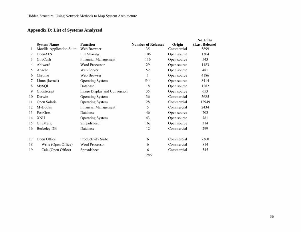
Hidden Structure: Using Network Methods to Map System Architecture
36
Appendix D: List of Systems Analyzed
System Name Function Number of Releases Origin
No. Files (Last Release)
1 Mozilla Application Suite Web Browser 35 Commercial 5899
2 OpenAFS File Sharing 106 Open source 1304
3 GnuCash Financial Management 116 Open source 543
4 Abiword Word Processor 29 Open source 1183
5 Apache Web Server 52 Open source 481
6 Chrome Web Browser 1 Open source 4186
7 Linux (kernel) Operating System 544 Open source 8414
8 MySQL Database 18 Open source 1282
9 Ghostscript Image Display and Conversion 35 Open source 653
10 Darwin Operating System 36 Commercial 5685
11 Open Solaris Operating System 28 Commercial 12949
12 MyBooks Financial Management 5 Commercial 2434
13 PostGres Database 46 Open source 703
14 XNU Operating System 43 Open source 781
15 GnuMeric Spreadsheet 162 Open source 314
16 Berkeley DB Database 12 Commercial 299
17 Open Office Productivity Suite 6 Commercial 7360
18 Write (Open Office) Word Processor 6 Commercial 814
19 Calc (Open Office) Spreadsheet 6 Commercial 545
1286

Hidden Structure: Using Network Methods to Map System Architecture
37
References
Akaikine, Andrei (2010) "The Impact of Software Design Structure on Product Maintenance Costs and Measurement of Economic Benefits of Product Redesign," S.M. thesis, System Design and Management Program, Massachusetts Institute of Technology.
Alexander, Christopher (1964) Notes on the Synthesis of Form, Cambridge, MA: Harvard University Press.
Baldwin, Carliss Y. and Kim B. Clark (2000). Design Rules, Volume 1, The Power of Modularity, Cambridge MA: MIT Press.
Barabasi, A. Scale-Free Networks: A Decade and Beyond, Science, Vol 325: 412-413
Braha, Dan., A.A. Minai and Y. Bar-Yam (2006) "Complex Engineered Systems: Science meets technology," Springer: New England Complex Systems Institute, Cambridge, MA.
Braha, Dan., and Y. Bar-Yam (2007) “The Statistical Mechanics of Complex Product Development: Empirical and Analytical Results,” Management Science, 53(7): 1127-1145.
Cai, Y., Wang, H., Wong, S., & Wang, L. (2013, June). Leveraging design rules to improve software architecture recovery. In Proceedings of the 9th international ACM Sigsoft conference on Quality of software architectures (pp. 133-142). ACM.
Chidamber, S.R. and C.F. Kemerer (1994) "A metrics suite for object oriented design," IEEE Transaction on Software Engineering, 20(6): 476-493.
Cataldo, Marcelo, Patrick A. Wagstrom, James D. Herbsleb and Kathleen M. Carley (2006) "Identification of Coordination Requirements: Implications for the design of Collaboration and Awareness Tools," Proc. ACM Conf. on Computer-Supported Work, Banff Canada, pp. 353-362
Cataldo, M., A. Mockus, J.A. Roberts and J.D. Herbsleb (2009) "Software Dependencies, Work Dependencies, and Their Impact on Failures," IEEE Transactions on Software Engineering, 35(6): 864-878.
Christensen, Clayton M. (1997) The Innovator's Dilemma: When New Technologies Cause Great Firms to Fail, Boston MA: Harvard Business School Press.
Clark, Kim B. (1985) "The Interaction of Design Hierarchies and Market Concepts in Technological Evolution," Research Policy 14 (5): 235-51.
Colfer, Lyra J. and Carliss Y. Baldwin (2010) "The Mirroring Hypothesis: Theory, Evidence and Exceptions," Harvard Business School Working Paper No. 10-058, January 2010 (revised, June 2010), available at http://papers.ssrn.com/sol3/papers.cfm?abstract_id=1539592 .
Conway, M.E. (1968) "How do Committee's Invent," Datamation, 14 (5): 28-31.
Csermely, Peter., Adras London, Ling-Yun Wu and Brian Uzzi (2013) “Structure and Dynamics of Core/Periphery Networks,” Journal of Complex Networks 1, 93-123.
David, Paul A. (1985) "Clio and the Economics of QWERTY," American Economic Review 75(2):332-337.
Dosi, Giovanni (1982) "Technological paradigms and technological trajectories," Research Policy, 11: 147-162
Eppinger, S. D., D.E. Whitney, R.P. Smith, and D.A. Gebala, (1994). "A Model-Based Method for Organizing Tasks in Product Development," Research in Engineering Design 6(1):1-13
Fixson, Sebastian K. and Jin-Kyu Park (2008). “The Power of Integrality: Linkages between Product Architecture, Innovation and Industry Structure,” Research Policy 37(8):1296-1316.
Garud, Raghu, Sanjay Jain and Arun Kumaraswamy (2002) "Institutional Entrepreneurship in the Sponsorship of Technological Standards: The Case of Sun Microsystems and Java," Academy of Management Journal, 45(1):196-214.
Gokpinar, B., W. Hopp and S.M.R. Iravani (2007) "The Impact of Product Architecture and Organization Structure on Efficiency and Quality of Complex Product Development," Northwestern University

Hidden Structure: Using Network Methods to Map System Architecture
38
Working Paper.
Henderson, R., and K.B. Clark (1990) "Architectural Innovation: The Reconfiguration of Existing Product Technologies and the Failure of Established Firms," Administrative Sciences Quarterly, 35(1): 9-30.
Holland, John H. (1992) Adaptation in Natural and Artificial Systems: An Introductory Analysis with Applications to Biology, Control and Artificial Intelligence, 2nd Ed. Cambridge, MA: MIT Press.
Kauffman, Stuart A. (1993) The Origins of Order, New York: Oxford University Press
Klepper, Steven (1996) “Entry, Exit, Growth and Innovation over the Product Life Cycle, American Economic Review, 86(30):562-583.
Lagerstrom, Robert, Carliss Y. Baldwin, Alan MacCormack, and David Dreyfus. "Visualizing and Measuring Software Portfolio Architectures: A Flexibility Analysis." Harvard Business School Working Paper, No. 14-083, March 2014.
LaMantia, Matthew J., Yuanfang Cai, Alan D. MacCormack and John Rusnak (2008) "Analyzing the Evolution of Large-Scale Software Systems using Design Structure Matrices and Design Rule Theory: Two Exploratory Cases," Proceedings of the 7th Working IEEE/IFIP Conference on Software Architectures (WICSA7), Vancouver, BC, Canada, February 18-22.
Langlois, Richard N. and Paul L. Robertson (1992). “Networks and Innovation in a Modular System: Lessons from the Microcomputer and Stereo Component Industries,” Research Policy, 21: 297-313, reprinted in Managing in the Modular Age: Architectures, Networks, and Organizations, (G. Raghu, A. Kumaraswamy, and R.N. Langlois, eds.) Blackwell, Oxford/Malden, MA.
Luo, J., Baldwin, C. Y., Whitney, D. E., & Magee, C. L. (2012). The architecture of transaction networks: a comparative analysis of hierarchy in two sectors. Industrial and Corporate Change, 21(6), 1307-1335.
MacCormack, Alan and M. Iansiti, (2009) "Intellectual Property, Architecture and the Management of Technological Transitions: Evidence from Microsoft Corporation," Journal of Product Innovation Management, 26: 248-263
MacCormack, Alan D. (2001). “Product-Development Practices That Work: How Internet Companies Build Software,” Sloan Management Review 42(2): 75-84.
MacCormack, Alan, Carliss Baldwin and John Rusnak (2012) "Exploring the Duality Between Product and Organizational Architectures: A Test of the "Mirroring" Hypothesis," Research Policy, 41(8): 1309-1324.
MacCormack, Alan, John Rusnak and Carliss Baldwin (2006) “Exploring the Structure of Complex Software Designs: An Empirical Study of Open Source and Proprietary Code,” Management Science, 52(7): 1015-1030.
Marple, D. (1961), “The decisions of engineering design,” IEEE Transactions of Engineering Management, 2: 55-71.
Mead, Carver and Lynn Conway (1980) Introduction to VLSI Systems, Addison-Wesley, Reading, MA.
Murmann, Johann Peter and Koen Frenken (2006) "Toward a Systematic Framework for Research on Dominant Designs, Technological Innovations, and Industrial Change," Research Policy 35:925-952.
Noble, David F. (1984) Forces of Production: A Social History of Industrial Automation, Oxford: Oxford University Press.
Rivkin, Jan W. (2000) “Imitation of Complex Strategies” Management Science 46:824-844.
Rivkin, Jan W. and Nicolaj Siggelkow (2007) "Patterned Interactions in Complex Systems: Implications for Exploration," Management Science, 53(7):1068-1085.
Sanderson, S. and M. Uzumeri (1995) "Managing Product Families: The Case of the Sony Walkman," Research Policy, 24(5):761-782.
Schilling, Melissa A. (2000). “Toward a General Systems Theory and its Application to Interfirm Product

Hidden Structure: Using Network Methods to Map System Architecture
39
Modularity,” Academy of Management Review 25(2):312-334, reprinted in Managing in the Modular Age: Architectures, Networks, and Organizations (G. Raghu, A. Kumaraswamy, and R.N. Langlois, eds.), Blackwell, Oxford/Malden, MA.
Sharman, D. and A. Yassine (2004) "Characterizing Complex Product Architectures," Systems Engineering Journal, 7(1).
Sharman, David, Ali Yassine and Paul Carlile (2002). “Characterizing Modular Architectures,” Proceedings of the ASME 14th International Conference on Design Theory & Methodology, DTM-34024, Montreal, Canada (September).
Simon, Herbert A. (1962) “The Architecture of Complexity,” Proceedings of the American Philosophical Society 106: 467-482, repinted in idem. (1981) The Sciences of the Artificial, 2nd ed. MIT Press, Cambridge, MA, 193-229.
Sosa, M. E., Mihm, J., & Browning, T. R. (2013). Linking Cyclicality and Product Quality. Manufacturing & Service Operations Management, 15(3), 473-491.
Sosa, Manuel, Steven Eppinger and Craig Rowles (2004) "The Misalignment of Product Architecture and Organizational Structure in Complex Product Development," Management Science, 50(12):1674-1689
Sosa, Manuel, Steven Eppinger and Craig Rowles (2007) "A Network Approach to Define Modularity of Components in Complex Products," Transactions of the ASME Vol 129: 1118-1129
Stein, Clifford, Robert L. Drysdale and Kenneth Bogart (2011) Discrete Mathematics for Computer Scientists, Boston, MA: Addison-Wesley.
Steward, Donald V. (1981) “The Design Structure System: A Method for Managing the Design of Complex Systems,” IEEE Transactions on Engineering Management EM-28(3): 71-74 (August).
Sturtevant, Daniel J. (2013) "System Design and the Cost of Architectural Complexity," Ph.D thesis, Engineering Systems Division, Massachusetts Institute of Technology.
Suarez, F and J.M. Utterback, (1995) Dominant Designs and the Survival of Firms, Strategic Management Journal, Vol. 16: 415-430
Thompson, James D. (1967) Organizations in Action: Social Science Bases of Administrative Theory, New York, NY: McGraw-Hill.
Tushman, Michael L. and Lori Rosenkopf (1992) "Organizational Determinants of Technological Change: Toward a Sociology of Technological Evolution," Research in Oragnizational Behavior Vol 14: 311-347
Tushman, Michael L. and Murmann, J. Peter (1998) "Dominant designs, technological cycles and organizational outcomes" in Staw, B. and Cummings, L.L. (eds.) Research in Organizational Behavior, JAI Press, Vol. 20.
Ulrich, Karl (1995) “The Role of Product Architecture in the Manufacturing Firm,” Research Policy, 24:419-440, reprinted in Managing in the Modular Age: Architectures, Networks, and Organizations, (G. Raghu, A. Kumaraswamy, and R.N. Langlois, eds.) Blackwell, Oxford/Malden, MA.
Utterback, James M. (1996) Mastering the Dynamics of Innovation, Harvard Business School Press, Boston, MA.
Utterback, James M. and F. Suarez (1991) Innovation, Competition and Industry Structure, Research Policy, 22: 1-21
Wasserman, S. (1994). Social network analysis: Methods and applications (Vol. 8). Cambridge university press.
Wilkie, F. G. and B. A. Kitchanham (1999) "Coupling Measures and Change Ripples in C++ Application Software," The Journal of Systems and Software, 52(2000): 157-164.
Xiao, L., Cai, Y. and Kazman, R. (2014) "Design Rule Spaces: A New Form of Architecture Insight," Manuscript.