Hidden symmetry and explicit spheroidal elgenfunctionsof the hydrogen atom

Stella M. Sung and Dudley R. HerschbachDepartment ofChemistry, Harvard University, Cambridge, Massachusetts 02138

(Received 17 June 1991; accepted 30 July 1991)

The Schrödinger equation for a hydrogenic atom is separable in prolate spheroidal coordinates,as a consequence of the “hidden symmetry” stemming from the fixed spatial orientation of theclassical Kepler orbits. One focus is at the nucleus and the other a distance R away along themajor axis of the elliptic orbit. The separation constant a is not an elementary function of Z orR or quantum numbers. However, for given principal quantum number n and angularmomentum projection m, the allowed values of a and corresponding eigenfunctions inspheroidal coordinates are readily obtained from a secular equation of order n — m. Weevaluate a ( n,m;ZR) and the coefficients g, (a) that specify the spheroidal eigenfunctions ashybrids of the familiar Inim) hydrogen-atom states with fixed n and m but different 1 values.Explicit formulas and plots are given for a and g, and for the probability distributions derivedfrom the hybrid wave functions, E,g, (a) Inlm), for all states up through n = 4. In the limitR -. these hybrids become the solutions in parabolic coordinates, determined simply bygeometrical Clebsch—Gordan coefficients that account for conservation of angular momentumand the hidden symmetry. We also briefly discuss some applications of the spheroidaleigenfunctions, particularly to exact analytic solutions of two-center molecular orbitals forspecial values of R and the nuclear charge ratio Z /Zb.

I. INTRODUCTION

The extraordinary n2 degeneracy of the nonrelativistichydrogen-atom energy levels manifests a “hidden” but well-known symmetry. In addition to the Hamiltonian H andorbital angular momentum 1, the Lenz vector a is a constantof the motion.’ Classically, for bound states the a vectorpoints along the major axis of the Kepler elliptic orbit and itslength is proportional to the eccentricity. Although 1 and ado not commute, the hybrid operators k + (1/2) (1 + a)and k — = (1/2) (1 — a) do. Furthermore, the operatorsk ± and k obey the commutation relations for angularmomentum. This allows bound state eigenfunctions specified by the complete set of commuting constants of the motion to be constructed simply as angular momentum eigenstates. The quantum Kepler problem is thereby solved bypurely geometrical means. The familiar nim) eigenfunctions in spherical polar coordinates correspond to a coupledrepresentation which simultaneously diagonalizes H, k,k, (k + kr), and the projection (k÷2 +k2); thelatter two operators coincide with 12 and l, respectively. Theequivalent but distinct eigenfunctions in parabolic coordinates correspond to an uncoupled representation which simultaneously diagonalizes H, k2÷, k, and the separateprojections k + and k — (tantamount to l and as); theseeigenfunctions are linear combinations of the familiar jnlm)hydrogen-atom states with fixed n and m but different! values, determined by Clebsch—Gordan coefficients.

In addition to spherical and parabolic coordinates, thehydrogenic Schrödinger equation is separable in prolatespheroidal coordinates, with one focus at the nucleus and theother located along the Lenz vector at a distance R away.These coordinates, ordinarily used for two-center problems

such as H2,serve to “dress the atom in molecular clothing.”In view of the myriad applications of hydrogenic eigenfunctions, it is curious that the spheroidal solutions have receivedscant attention; e.g., graphs of them seem not to exist elsewhere. Previously, general features have been explored byCoulson and Robinson,5who noted that the limits R -.0 andR .-. co yield the spherical and parabolic solutions, respectively. Robinson6 also showed that the spheroidal solutionsprovide the correct zero-order basis states for treating theinteraction of a point charge or a point dipole with the hydrogen atom. Demkov7 used the spheroidal eigenfunctionsto construct analytic solutions (exact for the Born—Oppenheimer problem) for an electron interacting with two nucleifor certain special values of the internuclear distance R andthe charge ratio ZQ/Zb. Other aspects of the spheroidal eigenfunctions were elucidated by Judd,8 particularly the connection to the four-dimensional spherical harmonics.

Here, we apply and extend these results to evaluate explicitly the spectrum of the separation constant a ( n,m,ZR)for the hydrogen atom in spheroidal coordinates and theeigenfunctions. These are obtained from a secular equationof order n — m which provides coefficients g, (a) for expansion of the spheroidal eigenfunctions in the usual I nim)states. In effect, the g, (a) functions interpolate between thecoupled and uncoupled representations and thereby play therole of generalized Clebsch—Gordan coefficients. We plotthese coefficients and the probability distributions for thehybrid wave functions, E,g, (a) I nim), for all states up thorough n = 4. We also briefly discuss some prospective applications. These include driven oscillator states created by interaction with an intense laser field,9 recently treated in atwo-center spheroidal basis;’° planetary excited states of

J. Chem. Phys. 95 (10), 15 November 1991 0021-9606/91/227437-1 2$03.00 © 1991 American Institute of Physics 7437

7438 S. M. Sung and D. R. Herschbach: Explicit spheroidal eigenfunctions

two-electron atoms;” computing tunneling splittings andelectronic exchange energy for excited states of the H molecule-ion;’2 and further exact solutions akin to those ofDemkov7 for special diatomic molecular orbitals.

II. COUPLED AND UNCOUPLED REPRESENTATIONS

Three consequences of the dynamical symmetry’ ofthe Kepler problem lead immediately to a geometrical solution,

(i) The pair of hybrid operators, k ± = (l/2)(I ± a)commute with H and with each other and behave as angularmomentum vectors.

(ii) The angular momentum and Lenz vectors are perpendicular, l•a = a•l = 0; hence

k2÷ =k =(l2+a2)ask2

so these operators have the same eigenvalues.(iii) The Hamiltonian can be written in terms of other

constants of the motion,

H= —(2k +2k’ +1y’, (2.1)

with energy in hartree units, angular momenta in units.These properties imply that simultaneous eigenstates existfor k, k + k, and k

— ; if these are denoted byt’mlkm+ ,km_),

kØ=k(k+l)b, k±b=m±b. (2.2)

The eigenvalues k =0, 1/2, 1, 3/2,... and m ± = — k,—k + l,...,k— 1,k.NowEq.(2.l)yie1dsH=Eb,with

(2.3)

so the principal quantum number n as (2k + 1) = 1,2,3For a given value of k, there are 2k + 1 different values ofboth m ÷ and m ,and therefore a total of (k + 1)2 =

different states with the same energy. Accordingly, the exceptional n2 degeneracy results from the presence of theLenz vector as a constant of the motion.

The eigenstates b of Eq. (2.2) pertain to the uncoupledrepresentation. Hence they are not eigenfunctions of the orbital angular momentum, 12 = (k. + k. ), although theyare eigenfunctions of the projection, l = (k + + k

—

with eigenvalue m = m + + m — , always an integer. In thecoupled representation, simultaneous eigenstates exist fork2÷ , k , 12, and 4; if these are denoted by ‘I’ = urn),

k’P=k(k+1)’V, 12Il=l(l+l)4I, 4’V=m’I’,

(2.4)

where 1 ranges in integer steps between 1= 0 tol=2k=(n—1)andm=—1,—l+1,...,l—l,LTheun-itary transformations relating the two equivalent descriptions are

and

Ilrn)= C(kkl;rn+m...rn)Ikrn+,krn_) (2.5)m + ,m —

Ikrn+ ,krn ) =2C(kkl;m÷ rn_ m)Ilm),

where the C’s are Clebsch—Gordan coefficients with twoequal arguments.’3”4Aside from specifying notation, this

n = 4, m = I n = 5, m

I2V

2/ [ /[/n, m = n . 2

I fl?i’ ‘V

FIG. 1. Matrices of Clebsch—Gordan coefficients for the transformationsbetween coupled and uncoupled representations, Eqs. (2.5) and (2.6).Here, k=1(n — 1) and m = m+ + m_. Rows correspond to coupledstates Iln), in increasing order of!; columns correspond to the uncoupledstates (m + ,m

— , ranging from (k,m — k on the left-hand side to(m — k,k on the right-hand side.

outline serves to emphasize how simple matters becomewhen the hybrid quasiangular momentum vectors, k + andk — , are regarded as the basic operators.

Figure 1 gives matrices of Clebsch—Clordan coefficients,sufficient to treat all hydrogenic states up through n = 5;those for higher states can likewise be evaluated from standard tables.’5 Rows correspond to the coupled states urn),in increasing order of!; columns correspond to the uncoupled states (rn + ,m

— , ranging from (k,m — k on the left-hand side to (rn — k,k on the right-hand side. Subsequently, we will examine both the coupled and uncoupled states inexplicit coordinate representations.

III. TWO-CENTER SPHEROIDAL EIGENSTATES

For an electron at distances r and r from two fixedCoulomb centers with charges Z0 and Zb a distance R apart,the wave function is separable in the form L(2)M(u)

(2.6) exp( ±irnc5),with2= (r +rb)/R andp=(r. rb)/Rthe spheroidal coordinates and qf’ the azimuthal angle aboutthe line between the centers. The separated equations for theL (2) and M(u) factors are

n ± 5, m = 0

rr rr rr.y 3vsr vr -v

IT rrrr2’ 0 •2 ‘Vif

is- IT I] IS-‘yr ‘Vi ° ‘VT yr

n = 4, m = 0

1/Y3[rs[T i[i2V5 rvr rVr 2V5

I I I IS S 5 5

3[r1/r1[r it2V5 2V5 2V5 2V5

I I 1 Is

n = 5, m =1

n = 3, in = 0

J. Chem. Phys., Vol.95, No. 10,15 November1991

S. M. Sung and D. R. Herschbach: Explicit spheroidal eigenfunctions 7439

TABLE I. Secular equations for Lenz vector eigenvalues.

n — m Secular equation

2 a,a,,,÷1 =4p234 a,,,a,,,+ia,,,+2a,,,+3=4p2(fl,,,+3a,,,a,,,+1+$,,,+2a,,,a,,,.3

+8,,,+,am+za,,,+3)— l44p4

Notation: p2 = Z2R2/n2,with Z the nuclear charge, R the internuclear distance, and n the principal quantum number. a,,, ma + rn(rn + 1); amA

—p2, where — A is theeigenvalue ofthe Lenz vector [cf. Eq. (1)1.

fl,=,8,(n,rn)m[(12—m2)(n2—!2)]/[(21— 1)(21+ 1)].

4

3 p+3d

L2L(2) + [A + (Za + Zb )R2 —p222]L(2) = 0 n nm Degeneracy

(3.1) 003 2

and 1 02

LM(1.i) + [_ A — (Za — Zb )RAU+p24u2]M(4u)= 0, 0 1 2(3.2)

2 0 i’)

where A is the separation constant and p2 = — ER 2 is an 1 I 1 6

energy parameter. The operator 0 2

d d m2 300L — (22 1’ — (33)

‘d2 22_i’ 2 1 0

and L, has the same form with the factor (22— 1) replaced 1 2 0

by(1 _2). The pairofequations forL(2) andM(is) are 0 3 0

commonly referred to as the two-center equations.’6For ahydrogenic atom, we take Z = Z and Zb = 0, and since 0 0 2 2

E = — Z2/n2 for the bound states of interest here, 1 0p2 = AZ 2R2/n2. The pair of two-center equations then be- 4

come the same equation with different ranges for the van- 0 1 lj

ables, 2 0 o11 1 0 3

LF(x)+[A+2pnx—p2x21F(x)=0. (3.4)0 2

Whenx=2(rangeltoaz),F(x)=L(2),andwhenx=/A 0 0 1 2(range — ito + 1), F(x) = M(1u); in either case L has the

1 0 &form of Eq. (3.3). For simplicity, henceforth we write 2

mmlml. Forp = 0, ifwetake,u = cos 8or2 = cosh 6, then 0 1 0)

Eq. (3.4) reduces to the eigenvalue equation for P7’ (x), theassociatedLegendrepolynomials,withA = — 1(1 + 1).Itis 1 — is 0 0 0 1

only necessary to extend Rodriques’s formula,j 2 m/2 ,, i + m FIG. 2. Degenerate energy eigenstates for each n sorted according torn = 0,

P7’ (p)= — fL ) (1 — 2) for Lu I s i, 1, 2,... (u,ir,S,,...) and according to eigenvalues of the separation constant

2’!! du’ ± m A (designated by the spheroidal quantum numbers nA and n,,), thereby

(3.5) specifying spheroidal eigenstates as hybrids of the usual spherical eigen

by replacing the (1—p2) factors with (2 2

— 1) for thestates.

range 2 I I. Therefore, for pO a solution of either two-center equation has the form5”6 c, = A —p2 + 1(1+ 1),

F(x)=exp(—px)c,P7’(x), (3.6) c,., = 2p(1+n+1)(1+m+l)

where the summation runs from 1= m to 1= n — 1. On substituting this into Eq. (3.4) and simplifying with the aid ofidentities linking polynomials of different 1, we obtain athree-term recursion relation for the coefficients,

C,c, + C, , c,, + C,_ , c,_, = 0,

with

Vr

2 —(2s÷2

(21+3)(l—n)(l—m)

= —2p(21— i)

As another consequence of the hidden dynamical symmetryof the hydrogen atom, Eq. (3.7) is invariant to interchang

(3.7) ing the quantum numbers n and m. This striking propertyhas been analyzed by Judd8 and related to the Lenz vector.

J. Chem. Phys., Vol.95, No. 10, 15 November1991

7440 S. M. Sung and D. A. Herschbach: Explicit spheroidal elgenfunctions

sU4pci

——

da

FIG. 3. Eigenvalues for separation constant a = A—

p2 of two-center equa

tions, as functions of ZR. The lower panel pertains to states with

n — in = 2; the middle panel to n — in = 3; the upper panel to ii — m = 4.

In accord with Fig. 2, eigenvalues are labeled by the Inim) states to which

the spheroidal Inam) reduces for R —.0, where a— 1(1 + 1). Indicated on

the right are values of (m + — in— ) which govern the R — limit, where

a—. — 2p(m + — 1n ). The ordinate is scaled by l/(2p + n) to remain

finite in both limits.

For each pair of values of n and m, the recursion relationgives a secular determinant of order n — m. The roots determine the eigenvalues of the separation constant A and thecorresponding {c, } which specify the eigenfunctions.

Figure 2 shows the resulting pattern ofspheroidal eigenstates up through n = 4. For each energy level there are ndegenerate spheroidal states with different m (denoted by a,ir, ô, ... form = 0, 1,2,...), each comprised ofa linear combination of the n — m terms in Eq. (3.6) for 1= m to1= n — 1. Also listed for each of the eigenstates are the

spheroidal quantum numbers n and nh,, which specify the

3 number of nodes in the 2 and theu coordinate, respectively.Table I gives the secular equations in terms of a = A —and Fig. 3 plots the eigenvalues as functions of ZR.

The secular determinants for the spheroidal eigenstatescan be symmetrized8such that c, = Q,g,, where

= ( — l)’[(21+ l)(l—m)!/

(1 + m)!(l + n)!(n —1— 1)!] 1/2 (3.8)

The recursion relation for the new coefficients g, is then

with

G1g,+G,÷,g,, +G,_,g,_, =0, (3.9)

— { [(1+l)2—m2][n2—(1+ 1)2] 11/2

1’(21+ l)(21+ 3)

J[12_m21[n2—12]}”2G,.1 =

(2!— l)(2l+ 1)

Table II gives formulas for the g1 coefficients and Fig. 4 plotsvalues ofg (normalized to sum to unity) as functions ofZRfor all eigenstates up through n = 4.

Simple results are obtained for both the small-R andlarge-R limits. For R —0, where a — — 1(1 + 1), only oneg,coefficient is nonzero for each eigenstate (so the normalized

1), and the corresponding values of n, 1, and m are usedto label that state. For R —, , wherea—’ — 2p(m + — m

— ), the eigenvalue becomes proportional to that for the z component of the Lenz vector’3 andthe g, become the Clebsch—Gordan coefficients of Eq. (2.6)and Table I. Accordingly, in Fig. 3 we have scaled the eigenvalues by a factor, 2p + is, in order to have finite limits forboth R —.0 and R —. m. In both Figs. 3 and 4, the limitingvalues are marked on the ordinate axis.

The relationship between the eigenstates in spheroidalcoordinates, designated as nam), and the customary states

in spherical coordinates, designated by nim), is extremelysimple,

and

Inam) = g,nIm), (3.10)

In1m)=g,Inam). (3.11)

Forgiven n and m, the sum in Eq. (3.10) extends from! = mtol= n — land thatinEq. (3.ll)overthen — mdistinctavalues. The symmetrized set of coefficients {g,} thus definesa unitary transformation between the spheroidal and spherical eigenstates, and has the role of generalized Clebsch—Gordan coefficients,

= namInlm) = (nlmlnam), (3.12)

in analogy to the angular momentum recoupling of Eqs.(2.5) and (2.6). In Appendix A we derive this relationship.It follows from the fact, as pointed out by Judd,8 that in thelimit of large 2 the spheroidal coordinates become polarspherical coordinates.

—l

—3

2

0

+p4

.1

+—I

+—‘

ZR

J. Chem. Phys., Vol. 95, No. 10, 15 November 1991

S. M. Sung and D. R. Herschbach: Explicit spheroidal eigenfunctions 7441

TABLE H. Spheroidal hybridization coefficients.

n — m g,(a,p) = (n!mlnam>

Any g,,, = const

2

3 g,,,..1/g,,, =l[(2m+3)/(m+2)]”(a,,,/p)

g,,,2/g,,, = [(m+ l)/(m+2)]”2(a,,,/a,,,÷2)

4 g,,,/g,,, =[4(2m+3)/(2m+5)]”2(a,,,/p)

g,,,÷2/g,,,=(m+1)(m+3)/3]”2[(a,,,a,,,÷1/12p2)(2m+3)—(2m+5)]

,,— I [(2m+3)(Zm+5)1v2[(2m+3) 611g,,,3 r—[

(m+l)(m+3) J Li2m+5 2P ) °1 a÷3

Notation as in Table I.

IV. EXPLICIT EIGENFUNCTIONS AND PROBABILITYDISTRIBUTIONS

The eigenstates in spheroidal coordinates (A,p,) aregiven explicitly by

Inam) =exp[ —p(2+p)]{(A2—l)(l _,12)}m/2

Xfnam(2)fnam(I1) exp( ±imcb), (4.1)

aside from normalization.5This form is obtained from Eq.(3.6) with the substitution

P7’(x) = 1x2— lImhZNmC2)(X),

where Nm ir”22- mr ( m + ), which replaces the associated Legendre function with a Gegenbauer polynomial,C”2(x). Accordingly, the polynomial factors innarn) are given by

fnam(X)=g,Q,C2)(x), (4.3)

aside from normalization. Again, for given n and rn, thereare n — m distinct values of a, and the sum extends from1= m to 1= n — 1. Table III gives these canonical polynomials for all eigenstates up through n = 4. Appendix B liststhe roots of the polynomials for these eigenstates for severalvalues of ZR.

Polar spherical coordinates (r,8,) and parabolic coordinates are related to the prolate spheroidal coordinates by

p=2p(2+u), pcos8=2p(l+2s),

p sin 8=2p[’:A2_ l)(l _2)]1/2,

wherep = 2Zr/n with (rr), and by

=p(2—l)(l—p), i=p(2+l)(l+p), (4.5)

with 2p = ZR In. With these substitutions, we find that theeigenfunctions I nim) in spherical coordinates and I nrm) inparabolic coordinates’7 contain the same factors as Eq.(3.13) except that fnam (2 )fnan, (ku) is replaced by

pl_n1L (p)C 1/2) (cos 8) (4.6)

or by

L’()L”(s), (4.7)

where L (x) is an associated Laguerre polynomial. In thespherical case, for each 1, the Laguerre factor has n — 1— 1radial nodes, and the Gegenbauer factor has 1— m angularnodes. The total number of nodes thus is it — m — 1, independent of the I value. In the parabolic case,s+ t= a= n—rn—I is again the total number of nodes.The other natural quantum number is s — t = r = — a,—o•+ 2,..., a— 2,a thisindexrremainsagoodquantum

number in the presence of a uniform electric field along the zaxis.’7 Hence for given n and rn there are n — m paraboliceigenstates related to spherical eigenstates in the same fashion as the spheroidal states designated in Fig. 2. Note thatinterchange of2 andi leaves Eqs. (4.6) and (4.7) invariant,since p, cos 8 and are invariant to this interchange. Wethus have three options for constructing the polynomial factors in the spheroidal eigenfunctions: from Eq. (4.3) as aproduct of two identical Gegenbauer functions; or from Eq.(4.6) as products of Laguerre and Gegenbauer functions,summed overt according to Eq. (3.10); or from Eq. (4.7) asproducts of two Laguerre functions, summed over the rquantum number.

In the limit R —, 0, each spheroidal eigenfunction narn)reduces to a particular spherical function I nlm), specified bya—. — 1(1 + 1). Likewise, in the limit R—. , each Inam)becomes a particular parabolic function Inrm), which inturn can be obtained from Eq. (3.10) as a linear combinationof spherical functions with the g, given by the Clebsch—Gor

(4 dan coefficients of Eq. (2.6) and Fig. 1. Other aspects of thetransition to these limits have been examined and illustratedby Coulson and Robinson.5

For the probability distributions, a format analogous tothat customary for spherical functions can be obtained fromEq. (3.10). In spherical coordinates the joint distributionobtained from the squared modulus (nam I nam) is not separable,

Pncxrn (p,O,c) = g1g,.pR1(p)pR,. (p)

(4.8)

(4.2)

J. Chem. Phys., Vol. 95, No. 10,15 November 1991

00

0.

14

.

11

1ti

ll

__

_____

8.4

8uI

0oP

.4

e___

_______

__________

__________

__

__

__

__

__

a1

1

.p

8—

i—.—

,..

I—i—

—i-

p.

I—.4—

ie

0,

0,

S. M. Sung and 0. R. Herschbach: Explicit spheroidal eigenfunctions 7443

TABLE III. Canonical polynomials.

n m f,,,Jx)

1 0 12 0 x—(2p/a)2 1 13 0 x’—l[(a+6)/p]x+[1+(8/a)j3 1 x—[2p/(a+2)]3 2 1

4 X3__F(+)lX2_ 12p2+a(a+18) (a+12)(52_a(a+2)]

2 1 p J d(p,a) 6pd(p,a)4 1 x2_l[(a+12)/plx+[(a+14)/(a+2))4 2 x—[2p/(a+6)l4 3 1

Notation as in Tables I and H, with d(p,a) = 20 — a(a + 2).

P,,m(8)=gIY,m(O,.b)I2,

where R, (p) is the usual normalized radial wave function2and Y,,,, (,ç) is a spherical arm5Figure 5 shows theradial probability distributions for all states up throughn = 4 for ZR = 0, 5, 15, 50, and . Of course the small-Rand large-R limits represent the familiar spherical and parabolic results, respectively. Figure 6 shows corresponding angular probability distributions for ZR = 0, 15, and on. Thevarious knobs and lobes that emerge or retreat as ZR is varied reflect the shifting pattern of nodes as the weighting factors g change. Particularly when the number of nodes,u = n — m — I, is large such plots resemble the polyhedraknown as “stellations,” but with rounded rather than spikylobes.’8 However, the probability distributions do not taketheir simplest or most revealing form in these spherical coordinates, since p and 0 involve sums and products of thespheroidal coordinates, according to Eq. (4.4). In particular, in Pfla,,, (6) the symmetry about the plane 0= 900 conceals the asymmetry about the p = 0 plane which exists inthe actual spheroidal eigenstates.

In terms of spheroidal coordinates, the probability distribution as obtained directly from Eq. (3.13) is separable,

with

Pnarn(2’I) = Pnczrn(2)Pnarn(I)’

V. DISCUSSION

Beyond providing an unconventional molecular perspective for the hydrogen atom, the spheroidal eigenfunctions have practical utility. As is well known, the paraboliceigenstates provide the correct zeroth-order linear combinations of the degenerate spherical eigenstates for treating theStark effect of the hydrogen atom in a uniform electricfield.’7 Although little known, the spheroidal eigenstateslikewise provide the correct zeroth-order hybrids, specifiedby the g, coefficients, for treating the Stark effect induced bya point charge or a point dipole.6 In the R —. limit, thisperturbation becomes equivalent to a uniform field and thespheroidal functions indeed reduce to the parabolic eigenstates.

Other applications arise when an hydrogenic atom issubject to a two-center perturbation. Such a situation in opti

(4.11) cal physics is exemplified in recent work ofPont and Gavrilaon hydrogen in a circularly polarized, high-intensity andhigh-frequency laser field.9 The coupling of the radiationfield with the atom produces a potential containing an additional time-dependent center, displaced from the nucleus bya distance proportional to the square root ofthe light intensity. The electron oscillates between the nucleus and this center, driven by the radiation. Consequently, the spheroidal

(4 10) ples for both x = p and x = 2. Others may be readily constructed from Table III, augmented by the list of zeros of the

f0m (x) polynomials given in Appendix B. In these coordinates, the nodal structure is rather simple and stable. Eacheigenstate nam) corresponds to particular values of thespheroidal quantum numbers (n2, np,, m, listed in Fig. 2),and thus the number of nodes in each of these coordinatesremains the same as R is varied.

nam(X)P(_2Pt)IX2_1Im[fnam(X)12,(4.12)

where again x represents p in the interval ( — 1,1) and represents 2 in the interval (1, on). Figure 7 shows a few exam-

J. Chem. Phys., Vol.95, No. 10, 15 November1991

7444 S. M. Sung and D. R. l-ferschbach: Explicit spheroidal eigenfunctions

o

3jw /4dir

3scr 9(\4P7t

i/i

___

ä•°f

__

2so 3pir ,f4ds

10 10 1520

0 5 10 15 20 0 5 190 15 20 0 5 l,O 15 20 0 5 I,D 15 20

FIG. 5. Radial probability distributions for the spheroidal hybrids up through n = 4, as specified in Eq. (4.9), for ZR = 0 (—), 5(-S-),

15 (-••-), 50 (•••),and (---). The lowest row shows the four eigenstates ofFig. 2 with n — m = 1; the next row shows the three pairs of eigenstates with n — = 2; the next

the two triplets with n — m = 3; the top row the quartet with n — m =4. The abscissa scale in each case pertains top = 2Zr/n, for the range p = 0 to 20.

J. Chem. Phys., Vol. 95, No. 10, 15 November1991

S. M. Sung and D. R. Herschbach: Explicit spheroidal elgenfunctions 7445

H

FIG. 6. Polar plots of angular probability distributions for the spheroidalhybrids up through n = 4, as specified in Eq. (4.10), for ZR = 0 (—), 15(),and (---). The layout corresponds to Fig. 5. The z axis is horizontal.

eigenfunctions provide an appropriate basis for treating sucha system.

Similarly, spheroidal eigenstates are appropriate for theexchange or tunneling of an electron between a pair of protons. This process has been treated extensively for the g,upairs of electronic states that stem from separated atomswith n = 1 and for all excited states with maximal values ofm =l=n — I aswe11.’ Thesecorrespondtothe lsu, 2pir,3d5, 4f,... states, as depicted in Figs. 2, 5, and 6, that do nothybridize with others of the same n when subject to a two-center perturbation; in effect, such states remain spherical.The spheroidal eigenstates offer a natural basis for treatingthe many other excited states that have less than maximal mvalues and strong hybridization. The spheroidal basis is implicit in asymptotic expansions in hR developed by Dam-burg and Propin” and by Cizek eta!.2° for the eigenvaluesof Hj states.

The spheroidal eigenstates also offer a convenientmeans to construct “elliptic” states with maximum localization on the classical Kepler orbits.2’ These involve a sumover m, in contrast to Rydberg atoms in “circular” states,22which correspond in the classical limit to an electron in acircular orbit and have the maximal value of m = 1= n — 1.Another natural application pertains to “planetary” statesof two-electron In such states, for which the principal quantum numbers of the electrons differ markedly(n, n2 ), the nodal structure of the eigenfunctions is foundto match closely that for the hydrogenic spheroidal eigenstates with n = n,. With allowance for the perturbationfrom the more distant electron,23 with n = n2, the spheroidal eigenstates should provide an efficient route to calculating emission lifetimes and other properties of the planetarystates.

The hydrogenic spheroidal eigenstates can be used toconstruct exact analytic solutions for special configurationsof the general two-center Coulombic system comprised of acharged particle interacting with a pair of fixed charges Z,andZ6 adistanceR apart.’6AsseeninEqs. (3.1) and (3.2),for this general problem the L (2) and M(p) factors of theeigenfunctions each satisfy similar equations, with the samevalues forp2and A but different parameters, (Za + Zb) and(Z0 — Zb), respectively. Thus, as noted by Coulson andRobinson,5 both factors may have hydrogenic forms if forsome pair ofprincipal quantum numbers n and n,, the energy eigenvalues are equal and the nodal structures correspondto hydrogenic states. The energy condition requires

E =— (Za + Z6)2/n = — (Z — Zb)2/n. (5.1)

The nodal condition for L (2) requires that the number ofnodesdoesnotexceednA — m — lintheinterval(l,co)andfor M(p) that it not exceed — m — 1 in the interval(— 1, + 1). The requirement that the separation constantmust be the same for both equations, A, = A, determinesthe specific internuclear distance .1? for which this hydrogenic solution of the two-center problem holds. Such solutions have been obtained for several electronic states byDemkov.7These solutions are simply products of two different hydrogenic spheroidal eigenfunctions, with the same values for a = A — p2, m, and R but different values for the

J. Chem. Phys., Vol.95, No.10, 15 November1991

7446 S. M. Sung and D. R. Herschbach: Explicit spheroidal elgenfunctions

........4

__

o

20 40 0 2040 0!\ 40

__ __

II

3w 3po [‘\ 3d

1

_________

/ \0LL- ..________ Sf

0 20 40 0 20 40 0 20 40

i1\o.:

20

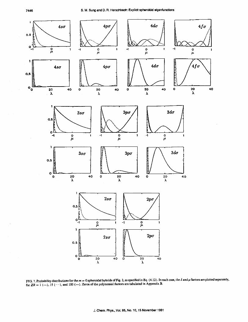
FIG. 7. Probability distributions for them = 0 spheroidal hybrids of Fig. 2, as specified in Eq. (4.12). In each case, the A and1sfactors are plotted separately,

for ZR = 1 (—), 15 (••), and 100 (•--). Zeros of the polynomial factors are tabulated in Appendix B.

J. Chem. Phys., Vol. 95, No. 10, 15 November 1991

S. M. Sung and D. R. Herschbach: Expflcit spheroidal eigenfunctions 7447

principal quantum numbers, nA and ng, related by(Za +Zb)/n = (4 —Z)/n,.

ACKNOWLEDGMENTS

We have enjoyed discussions with John Briggs, DonFrantz, Sabre Kais, Mario Lopez, and particularly with JanRost. We are grateful for an NSF Fellowship (to S. M. S.)and for support received from the Venture Research Unit ofthe British Petrolelum Company.

APPENDIX A: RELATION OF SEPARATION CONSTANTTO LENZ VECTOR

Coulson and Joseph24 have evaluated in a convenientform the operator FA corresponding to the separation constantA of the two-center equations, Eqs. (3.1 )—( 3.2); for thecase Za = Z and Z,, = 0, the hydrogenic atom, this gives

the eigenvalue relation

FA’I’=AW with W=L(2)M(u),

where

FA = — [12 + R ( — 2E)“2a — R2E],

(Al)

(A2)

and 1 is the orbital angular momentum, a the Lenz vector,and E = — Z2/n2 the bound-state energy. In terms of theenergy parameterp2 = — ER , this becomes

FA— —(12+2pa—p2). (A3)

In the text, we set up the secular determinant for thespheroidal eigenstates, Eq. (3.9), to obtain the eigenvaluesa = A

—p2 of the separation constant and the {g1} coeffi

cients, by expanding the eigenfunctions 4’ of Eq. (Al) inassociated Legendre polynomials, according to Eq. (3.6).Since n and m remain good quantum numbers, the spheroi

TABLE IV. Zeros off,,,,,, (x) polynomials.

dal eigenstates Inam) must be related to the usual sphericaleigenstates nim) by a unitary transformation of the form ofEqs. (3. l0)—(3 1.2); it is only necessary to demonstrate thatthe {g,} obtained from Eq. (Al) are the appropriate coefficients. However, in the limit 2—. o, it is readily shown5 thatthe spheroidal coordinates become polar coordinates:2—2r/R and4u—cos 0. Then L(2)M(4u) for a given a becomes a linear combination of the R, (p )P 7’ (0), summedover 1. From this it follows that the {g,} coefficients indeedspecify the unitary transformation.

Judd8 has shown that a recursion relation identical toEq. (3.9) appears when a operates on a four-dimensionalspherical harmonic.25 Consequently, an equivalent procedure for solving Eq. (Al) is to expand 4’ in four-dimensionalspherical harmonics, and the same {g, } coefficients specifythis expansion. Other elegant properties that arise because 1and a are generators of the four-dimensional rotation grouphave been amply discussed.413’26’27

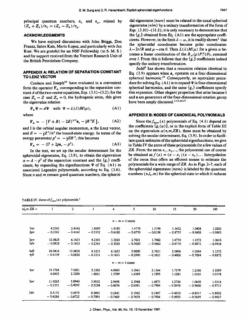
APPENDIX B: NODES OF CANONICAL POLYNOMIALS

Since the fnam (x) polynomials of Eq. (4.3) depend onthe coefficients {g, (a) }, or in the explicit form of Table IIIon the eigenvalues a (n,m,ZR), these must be obtained bysolving the secular determinant, Eq. (3.9). In order to facilitate quick estimates ofthe spheroidal eigenfunctions, we givein Table IV the zeros of these polynomials for a few values ofZR. From the zeros x1,x2,..., the polynomial can of coursebe obtained as 1(x) = (x — x1 )(x —x2).... Interpolationof the zeros thus offers an efficient means to estimate thepolynomials for a wide range of ZR. As in Figs. 2—7, each ofthe spheroidal eigenstates Inam) islabeled by the quantumnumbers (n,10.m) for the spherical state to which it reduces

nl0mZR= 1 2 3 4 5 10 15 50 100

n — m = 2 states

2scr 4.2361 2.4142 1.8685 1.6180 1.4770 1.2198 1.1422 1.0408 1.02022pcr 0.2361 —0.4142 —0.5352 —0.6180 —0.6770 —0.8198 —0.8755 —0.9608 —0.9803

3pir 2.0828 6.1623 4.2361 3.3028 2.7621 1.7662 1.4770 1.1272 1.06183dir 0.0828 —0.1623 —0.2361 —0.3028 —0.3620 —0.5662 —0.6770 —0.8872 —0.9418

4d6 24.0416 12.0828 8.1231 6.1623 5.0000 2.7621 2.0806 1.2684 1.12724J —0.4159 —0.0828 —0.1231 —0.1623 —0.2000 —0.3621 —0.4806 —0.7884 —0.8872

n — = 3 states

3scr 14.3768 7.4201 5.1563 4.0485 3.3961 2.1364 1.7379 1.2106 1.10394.0433 2.3200 1.8061 1.5709 1.4389 1.1995 1.1281 1.0362 1.0178

3po- 11.9265 5.8940 3.9032 2.9408 2.3948 1.4871 1.2764 1.0658 1.0314—0.2351 —0.4095 —0.5254 —0.6034 —0.6581 —0.7904 —0.8458 —0.9450 —0.9713

3dc, 0.5172 0.4476 0.3691 0.2841 0.1962 0.1487 —0.4010 —0.8017 —0.8992— 0.6286 — 0.6722 — 0.7093 — 0.7409 — 0.7678 — 0.7904 — 0.8955 — 0.9659 — 0.9827

J. Chem. Phys., Vol.95. No. 10, 15 November1991

7448 S. M. Sung and D. R. Herschbacft Explicit spheroidal elgenfunctions

TABLE IV. (Continued.)

nl0inZR= 1 2 3 4 5 10 15 50 100

4pir 29.0677 14.5969 9.8305 7.4715 6.0725 3.3565 2.5019 1.4060 1.1965

11.1413 5.6953 3.9282 3.0746 2.5816 1.6790 1.4192 1.1093 1.0527

4dir 24.0000 12.0027 8.0086 6.0187 4.8331 2.5492 1.8822 1.1885 1.0868

— 0.8269 — 0.1618 — 0.2345 — 0.2996 — 0.3568 — 0.5492 — 0.6522 — 0.8625 — 0.9260

4fir 0.4129 0.3767 0.3387 0.2993 0.2587 0.0516 —0.1313 —0.6544 —0.8186

0.4795 —0.5099 —0.5382 —0.5646 —0.5892 —0.6871 —0.7533 —0.9069 —0.9513

n — m = 4 states

4so- 31.2034 15.8167 10.7385 8.2216 6.7231 3.8545 2.8135 1.5201 1.2562

13.4038 6.9349 4.8336 3.8068 3.2028 1.9399 1.6725 1.1902 1.0935

3.9831 2.2909 1.7868 1.5563 1.4270 1.2130 1.1234 1.0345 1.0170

4p 28.8605 14.3433 9.5127 7.1200 5.7075 3.0337 2.2400 1.3059 1.1448

10.9840 5.4266 3.5972 2.7177 2.2229 1.4150 1.2317 1.0529 1.0249

—0.2348 —0.4078 —0.5220 —0.5981 —0.6511 —0.7777 —0.8310 —0.9330 —0.9636

4dy 23.9859 11.9706 7.9537 5.9360 4.7195 2.3138 1.6330 1.1002 1.0445

0.5169 0.4465 0.3666 0.2802 0.1915 —0.1714 —0.3729 —0.7584 —0.8715

— 0.6285 — 0.6716 — 0.7082 — 0.7393 — 0.7658 — 0.8490 — 0.8883 — 0.9583 — 0.9779

4fo 0.7570 0.7375 0.7159 0.6918 0.6651 0.4877 0.2612 — 0.5213 — 0.7539

—0.0416 —0.0829 —0.1236 —0.1634 —0.2022 —0:3748 —0.5075 —0.8247 —0.9102

—0.7904 —0.8047 —0.8177 —0.8295 —0.8402 —0.8815 —0.9088 —0.9682 —0.9837

See Appendix B.

for R -.0, where a —.‘.l (l + 1). The zeros located at valuesof x> I pertain to the A coordinate; those at — I <x< I pertain to the p coordinate. The number of zeros in 2 or p isgiven by the spheroidal quantum numbers, n,t or n, respectively, and remains the same as ZR is varied.

‘W. Pauli, Z. Phys. 36, 336 (1926).2L. I. Schiff, Quantum Mechanics, 3rd ed. (McGraw-Hill, New York,

1968), pp. 236—239.G. Baym, Lectures on Quantum Theory (Benjamin/Cummings, Reading,MA, 1969), pp. 175—179.

‘M. I. Englefield, Group Theory and the Coulomb Problem (Wiley-Inter-science, New York, 1972).5C. A. Coulson and P. D. Robinson, Proc. Phys. Soc. London 71, 815

(1958).6P. D. Robinson, Proc. Phys. Soc. London 71, 828 (1958).7Yu. N. Demkov, Pis’ma Zh. Eksp. Teor. Fix. 7, 101 (1968) [JETP Lett. 7,76(1968)].8B. R. Judd, Angular Momentum Theory for Diatomic Molecules (Academic, New York, 1975), Pp. 56—58, 67—73, 8 1—84.9M. Pont, Phys. Rev. A 40, 5659 (1989); M. Pont and M. Gavrila, Phys.

Rev. Lett. 65, 2362 (1990).‘°A. Frantz, H. KIar, and 3. S. Briggs, J. Opt. Soc. Am. B 4, MS (1989).flJ M. Rost and J. S. Briggs, J. Phys. B (in press).

12S. Kais, J. D. Morgan, and D. R. Herschbach, 3. Chem. Phys. (in press).“J. W. B. Hughes, Proc. Phys. Soc. London 91, 810 (1967).‘4F. Penent, D. Delande, and 3. C. Gay, Phys. Rev. A 37, 4707 (1988).‘5R. N. Zare, Angular Momentum (Wiley, New York, 1988).‘6E Teller and H. L. Sahlin, in Physical Chemistry—An Advanced Treatise,

edited by H. Eyring, D. Henderson, and W. Jost (Academic, New York,1970), Vol. 5, pp. 35—124. For subsequent work on H, seeD. D. Frantz

and D. R. Herschbach, J. Chem. Phys. 92, 6668 (1990), and papers citedtherein.

‘L. D. Landau and E. M. Lifshitz, Quantum Mechanics (Pergamon, London, 1958), pp. 121—125, 130—132, 251—256.

8S T. Coffin, The Puzzling World ofPolyhedral Dissections (Oxford University, Oxford, 1990), p. 83.

“R. J. Damburg and R. K. Propin, 3. Phys. B 1, 681 (1968).20J. Cizek, R. J. Damburg, S. Grafli, V. Grecchi, E. M. Harrell, J. G. Har

ris, S. Nakai, J. Paldus, R. K. Propin, and H. J. Silverstone, Phys. Rev. A33, 12 (1986).

21 3.-C. Gay, D. Delande, and A. Bommier, Phys. Rev. A 39, 6587 (1989).22R. 0. Hulet and D. Kleppner, Phys. Rev. Lett. 51, 1430 (1983).23P. A. Braun, V. N. Ostrosvsky, and N. V. Prudov, Phys. Rev. A 42, 6537

(1990).24C. A. Coulson and A. Joseph, Proc. Phys. Soc. London 90, 887 (1967).2S J Avery, Hyperspherical Harmonics: Applications in Quantum Theory

(Kluwer Academic, Dordrecht, 1989).26L. C. Biedenharn, 3. Math. Phys. 2,433 (1961).27D. R. Herrick, Phys. Rev. A 26, 323 (1982).

J. Chem. Phys., Vol.95, No. 10, 15 November1991