hierarchical bayesian auto-regressive models for...
TRANSCRIPT

Hierarchical Bayesian auto-regressive models for large space
time data with applications to ozone concentration modelling
Sujit Kumar Sahu∗
School of Mathematics, University of Southampton,
Southampton, SO17 1BJ, UK.
Khandoker Shuvo Bakar
CSIRO Mathematics, Information and Statistics,
GPO Box 664, Canberra, ACT 2601, Australia.
Increasingly large volumes of space-time data are collected everywhere by mobile
computing applications, and in many of these cases temporal data are obtained by
registering events, for example telecommunication or web traffic data. Having both
the spatial and temporal dimensions adds substantial complexity to data analysis and
inference tasks. The computational complexity increases rapidly for fitting Bayesian
hierarchical models, as such a task involves repeated inversion of large matrices. The
primary focus of this paper is on developing space-time auto-regressive models under
the hierarchical Bayesian setup. To handle large data sets, a recently developed
Gaussian predictive process approximation method (Banerjee et al. [1]) is extended
to include auto-regressive terms of latent space-time processes. Specifically, a space-
time auto-regressive process, supported on a set of a smaller number of knot locations,
is spatially interpolated to approximate the original space-time process. The resulting
model is specified within a hierarchical Bayesian framework and Markov chain Monte
Carlo techniques are used to make inference. The proposed model is applied for
analysing the daily maximum 8-hour average ground level ozone concentration data
from 1997 to 2006 from a large study region in the eastern United States. The
developed methods allow accurate spatial prediction of a temporally aggregated ozone
summary, known as the primary ozone standard, along with its uncertainty, at any
unmonitored location during the study period. Trends in spatial patterns of many
features of the posterior predictive distribution of the primary standard, such as
the probability of non-compliance with respect to the standard, are obtained and
illustrated.
Keywords: Bayesian inference, big-n problem, Gaussian predictive process, ozone
concentration, space-time modelling.
∗Corresponding Author. Email: [email protected]
1

1 Introduction
Many organisations collect spatial and spatio-temporal data routinely and on a regular
basis for a variety of reasons. It has been estimated that up to 80% of all data stored
in corporate databases may have a spatial component [2]. To gather intelligence from
such large space-time data and to fully exploit the space-time dependencies for making
predictive inference, there is an urgent need to develop fast and efficient statistical
methods capable of handling large data sets. Spatio-temporal models, specified at the
highest spatial and temporal resolutions, provide the capability for making inference
at any aggregate spatial and/or temporal levels. For example, a model specified for
the daily data can easily be aggregated to make inference on monthly or annual time
scales and can also allow one to estimate the associated uncertainties in a coherent
manner. Similarly, data modelled on a high resolution spatial scale can easily shed
inferential light on any spatially aggregated quantity.
Incorporating both spatial and temporal correlations into the Bayesian hierar-
chical models is a challenging task, but this is the one that is receiving increasing
interests from modellers from many fields of research and applications, see e.g., the
recent book by Cressie and Wikle [3] and the references therein. Hierarchical dy-
namical spatio-temporal models are often specified to achieve the various modelling
objectives. This paper will focus on the hierarchical auto-regressive models, see e.g.,
Sahu et al. [4] as a simpler sub-class of the dynamical spatio-temporal models since
these are often found to be the best models among a large class of models under a
variety of model choice and predictive model validation criteria, see e.g., [5]. Sahu and
Bakar [6] show that these models also enjoy superior theoretical predictive properties
and they also fit and validate better in real life modelling situations.
The hierarchical auto-regressive models, however, are not suitable for analysing
large data sets observed over vast study regions such as the eastern United States
(US). The problem here lies in inverting high dimensional spatial covariance matrices
repeatedly in iterative model fitting algorithms. This is known as the big-n problem
in literature (see e.g., Banerjee et al. [7]). The early approaches to solve the big-
n problem are mostly ad-hoc as some data are either un-used or repeatedly used,
e.g., [8] uses local kriging, [9] proposes subsampling from a large spatial dimension
by a moving window approach. The gradual methodological improvement comes
from the use of different approximation techniques of kriging equations, see e.g., a
space-filling approach with geo-additive models by [10], a moving average technique
by [11], and techniques based on using basis functions by [12]. Approaches based
on spectral analysis to approximate the likelihood function have also been proposed
by many authors, see e.g., [13] and [14]. Hartman and Hossjer [15] propose another
technique based on efficient computations using sparse matrix calculation algorithms
by exploiting the Gaussian Markov random fields ([16]) approximations. Reich et al.
[17] use a spatial quantile regression approach by considering a non-Gaussian process
2
in their models. They are able to reduce the dimension of the data by hierarchical
modelling of a smaller number of estimated quantile parameters from the original
observations.
Multi-resolution spatial models, see e.g., [18], [19], [20] are also able to provide
fast model fitting and can also capture non-stationarity in the data. However, these
models can be problematic to capture possible heterogeneity effects across vast spatial
regions. Modelling spatial covariance functions with a low rank matrix ([21]) and
a moderate rank matrix ([22]), fixed rank kriging ([23], [24]) can also handle the
large data sets but there are several problems associated with the choice of the basis
functions and their interpretations. A simpler approach based on an approximation
using the Gaussian predictive processes (GPP) for modelling multivariate spatial data
has been proposed by Banerjee et al. ([1]) and later on modified by [45]. This method
does not require sub-sampling of the data and neither does it require specification of
complex spatial basis functions.
Motivated by the need to model large data sets, this paper extends the GPP
approximation technique of [1] to include auto-regressive terms of the latent under-
lying space-time process. This auto-regressive process is defined at a set of a smaller
number of knot locations within the study region and then spatial interpolation, i.e.
kriging, is used to approximate the original space-time process. The model is fully
specified within a hierarchical Bayesian setup and is implemented using Markov chain
Monte Carlo (MCMC) techniques.
The paper illustrates the method by analysing a very large data set that recorded
the daily maximum 8-hour average ground level ozone concentration from 1997 to
2006 from a large number of monitoring sites located in the eastern US. Results from
this study include a spatially interpolated model based map, first of its kind to our
knowledge, showing the probability of non-compliance with respect to the primary
standard in each of the years 1999-2006. The paper also compares the predictive
performance of the GPP based model and the fully specified AR model of [4] using a
moderately large subset of the full data set where both models are feasible. There is
a considerable literature on space-time modeling of ground level ozone see e.g., [25],
[26], [27], [28], [29], [30], [31], [32], and [33]. However, none of these articles model
daily ozone concentration data for ten years observed over our study region of the
eastern US using space-time models.
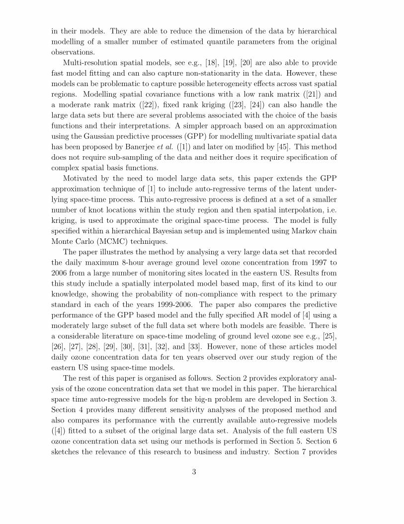
The rest of this paper is organised as follows. Section 2 provides exploratory anal-
ysis of the ozone concentration data set that we model in this paper. The hierarchical
space time auto-regressive models for the big-n problem are developed in Section 3.
Section 4 provides many different sensitivity analyses of the proposed method and
also compares its performance with the currently available auto-regressive models
([4]) fitted to a subset of the original large data set. Analysis of the full eastern US
ozone concentration data set using our methods is performed in Section 5. Section 6
sketches the relevance of this research to business and industry. Section 7 provides
3

a few summary remarks and an appendix contains the full conditional distributions
needed for implementing the Gibbs sampler.
2 Exploratory analysis
We consider the daily maximum 8-hour average ozone concentration data obtained
from 691 monitoring sites in our study region in the eastern US. These sites are
made up of 646 urban and suburban monitoring sites known as the National Air
Monitoring Stations/State and Local Air Monitoring Stations (NAMS/SLAMS) and
45 rural sites monitored by the Clean Air Status and Trends Network (CASTNET).
Out of the total 691 sites we set aside data from 69 randomly chosen sites for model
validation purposes and use the data from the remaining 622 sites to fit the models.
To relate ozone concentration with meteorological data we also have collected data
from 746 weather monitoring sites within the study region. Figure 1 provides a map
of the locations of these modelling, validation and weather monitoring sites.
We analyse daily data for T = 153 days in every year during May to September
since this is the high ozone season in the US. We consider these data for the 10
year period from 1997 to 2006 that allows us to study trend in ozone concentration
levels. Thus we have a total of 1, 057, 230 observations and among them approximately
10.44% are missing which we assume to be at random, although there are some annual
variation in this percentage of missingness.
The daily ozone concentration levels range from 0.22 to 246.22 in parts per billion
(ppb) with a mean of 50.41 ppb. Figure 2 provides a side by side boxplot of the daily
measurements for the 691 sites for each of the 10 years. The plot shows a general
decreasing trend from 1997 to 2001, a peak in the year 2002 and then a decreasing
trend until 2004. Slightly higher levels are seen in the last two years 2005 and 2006.
We model ozone on the square-root scale since it encourages symmetry and variance
stabilisation (see e.g., [4] and references therein), although other transformations such
as the logarithm is possible.
The main purpose of the modelling exercise here is to assess compliance with
respect to the primary ozone standard that states that the 3-year rolling average
of the annual 4th highest daily maximum 8-hour average ozone concentration levels
should not exceed 85 ppb, see e.g., [4]. Figure 3 plots the 4th highest maximum and
their 3-year rolling averages with a superimposed horizontal line at 85. As expected,
the plot of the rolling averages is smoother than the plot of the annual 4th highest
maximum values. The plots show that many sites are compliant with respect to the
standard, but many others are not. In addition, the plot of the 3-year rolling averages
shows a very slow downward trend. Both the plots show the presence of a few outlier
sites which are perhaps due to site specific issues in air pollution, for example due to
natural disasters such as forest fires.
4

We consider three meteorological variables: daily maximum temperature in degree
centigrade, relative humidity and wind speed as covariates for modelling the ozone
concentration levels, following [34] and [4] who found these three to be the most
significant explanatory variables, see also [29]. These three variables, however, have
been observed at the 746 meteorological sites which do not coincide with the ozone
monitoring sites (see Figure 1). Moreover, we need to have the values of these ex-
planatory variables at a number of unmonitored sites for prediction purposes. We use
simple kriging independently for the three meteorological variables using the fields
package in R ([35]). This method is known to under-estimate the uncertainty in the
predictions, see e.g., [17]. To address these concerns [36] considers a multiple kriging
method where a new predictive value for each variable is generated independently
at each MCMC iteration from the underlying estimated model for kriging. In this
paper, however, we only report the results based on a single kriged value for each
meteorological variable. Sahu et al. [4] detail a method where the covariate values at
each time point are imputed using a separable multivariate spatio-temporal model.
However, their approach is not suitable for the big-n problem of the current paper as
discussed in the introduction. In their modelling developments, [4] use differences in
successive day’s meteorology as the covariates instead of the observations themselves
so that the auto-regressive model using previous day’s ozone levels can be adjusted by
increment in meteorological values. In our modelling developments below we are not
required to specify the models using the meteorological increments since we specify
the auto-regressive models for random effects.
3 Models
Let Zl(si, t) denote the observed value of the response, possibly after a transformation,
at location si, i = 1, . . . , n on day t within year l for l = 1, . . . , r and t = 1, . . . , T .
These two time indices can also be used to specify the hour within day or day within
month and so on. Let Zlt = (Zl(s1, t), . . . , Zl(sn, t))′. Further, suppose that xlj(s, t)
denotes the value of the jth covariate, j = 1, . . . , p on day t in year l and let
Xlt =
x′
l(s1, t)...
x′
l(sn, t)
.
With these general notations several versions of auto-regressive models are described
next.
5

3.1 Auto-regressive models developed by Sahu et al. [4]
We first write down the hierarchical auto-regressive models developed in [4]. The first
stage of their modelling hierarchy assumes the measurement error model:
Zlt = Olt + ǫlt, l = 1, . . . r, t = 1, . . . , T, (1)
where ǫlt = (ǫl(s1, t), · · · , ǫl(sn, t))′ ∼ N(0, σ2
ǫ I). Here Olt = (Ol(s1, t), . . . , O(sn, t))′
denotes the true value corresponding to Zl(si, t) where
Olt = ρOlt−1 +Xltβ + ζlt, l = 1, . . . r, t = 1, . . . , T. (2)
where ζlt = (ζl(s1, t), . . . , ζl(sn, t))′ and we assume that ζlt ∼ GPn(0, σ2ψ(d;φ)) where
GPn(0, σ2ψ(d;φ)) denotes the n-dimensional Gaussian process with mean 0 and co-
variance function given by σ2ψ(d;φ) where σ2 and φ denote the common spatial
variance and the decay parameter, respectively and d denotes the distance. Here
ψ(d;φ) denotes the correlation function which we take to be the exponential correla-
tion function ψ(d;φ) = exp(−dφ) in our illustration, although other choices can be
adopted. The initial condition is given by
Ol0 = γ l + µl1, l = 1, . . . r, (3)
where 1 is the vector of dimension n with all elements unity and γ l = (γl(s1), . . . , γl(sn))′
is assumed to follow GPn(0, σ2l ψ(d;φ0)) independently for each l = 1, . . . , r. Note that
these initial random variables Ol(si, 0) are centred at µl and not at zero since Ol(si, 0)
represent the true response. The model is completed by assuming µl ∼ N(0, 104) and
proper inverse gamma prior distributions independently for each σ2l , see [4] for further
details. Henceforth, we shall denote this version of the AR models as ARHIER.
This version of the AR models is not suitable for adaptation with the GPP ap-
proximation proposed by [1] since each Zl(si, t) is paired with a true level Ol(si, t)
that cannot be reduced in dimension. Next we develop a modified version of these
models that will enable us to reduce the dimension of the random effects.
3.2 Modified hierarchical auto-regressive models
The ARHIER model assumes the AR model for the true values of the modelled
response Olt. Following [37] we modify this model so that the modified version does
not assume a true level Ol(si, t) for each Zl(si, t) but instead assumes a space-time
random-effect denoted by ηl(si, t). It then assumes an AR model for these space-time
random effects.
The top level general space-time random effect model is assumed to be:
Zlt = Xltβ + ηlt + ǫlt, l = 1, . . . r, t = 1, . . . , T. (4)
6

where ǫlt ∼ N(0, σ2ǫ I) where I is the identity matrix. In the next stage of the
modelling hierarchy the AR model is assumed as:
ηlt = ρηlt−1 + δlt, (5)
where δlt ∼ GPn(0, σ2ψ(d;φ)). The initial condition is assumed to be:
ηl(si, 0) ∼ GPn(0, σ20ψ(d;φ0)) (6)
where σ20 and φ0 are unknown parameters.
Note that the marginal mean of the random effects ηlt is zero, but the conditional
mean given ηlt−1 is no longer zero due to the auto-regressive specification (5). This
specification also implies a non-stationary marginal covariance function for ηlt that
does not need to be explicitly derived nor is it required since model fitting proceeds
through the conditional specification (5). Lastly, we note that higher order auto-
regressive terms can be included in (5). However, those are not considered here since
their inclusion will only weaken both the spatial and lag-1 temporal correlations
without providing significant additional descriptive ability.
3.3 Auto-regressive models with GPP approximations
The auto-regressive models specified in Section 3.2 create a random effect ηl(si, t)
in (4) corresponding to each data point Zl(si, t). This will lead to the big-n problem,
as discussed in the Introduction when n is large. To overcome this problem we propose
a dimension reduction technique through a kriging approximation following [1] as
follows. The main idea here is to define the random effects ηl(si, t) at a smaller number
of locations, called the knots, and then use kriging to predict those random effects at
the data locations. The auto-regressive model is only assumed for the random effects
at the knot locations and not for all the random effects at the observation location.
The method proceeds as follows.
At the top level we continue to assume the model (4), but we do not specify
ηlt directly through the auto-regressive model (5). Instead, we select m << n knot
locations, denoted by by s∗1, ..., s∗
m within the study region and let the spatial random
effects at these locations at time l and t be denoted by wlt = (wl(s∗
1, t), . . . , wl(s∗
m, t))′.
Discussion regarding the choice of these locations is given in Section 4.1. Assuming
an underlying Gaussian process independently at each time point l and t, [1] show
that the process ηlt can be approximated by
ηlt = Awlt (7)
with A = CS−1w where C denotes the n by m cross-correlation matrix between ηlt and
wlt, and Sw is the correlation matrix of wlt. Note that the common spatial variance
parameter does not affect the above since it cancels in the product CS−1w . Also, there
7

is no contribution of the means of either ηlt or wlt in the above since those means are
assumed to be 0.
The proposal here is to use the GPP approximation ηlt instead of ηlt in the top
level model (4), thus we assume that:
Zlt = Xltβ + ηlt + ǫlt, l = 1, . . . r, t = 1, . . . , T, (8)
where ηlt is as given in (7). Analogous to (5), we specify wlt at the knots conditionally,
given wlt−1, by
wlt = ρwlt−1 + ξlt, (9)
where ξlt ∼ GPm(0, σ2wψ(d;φ)) independently. Again we assume that wl0 ∼ N(0, σ2
l S0)
independently for each l = 1, . . . , r, where the elements of the covariance matrix S0
are obtained using the correlation function, ψ(d;φ0), i.e. the same correlation func-
tion as previously but with a different variance component for each year and also
possibly with a different decay parameter φ0 in the correlation function. Henceforth,
we shall call this model ARGPP.
A few remarks are in order. The above modelling specifications are justified using
the usual hierarchical modelling philosophies in the sense that the top level model is a
mixed model with mean zero random effects and these random effects have structured
correlations as implied by the spatial auto-regressive model at the second stage (9).
These two model equations, together with the initial condition, however, are neither
intended to, nor will ever exactly imply the auto-regressive model (5) for the original
random effects ηlt except for trivial cases such as the one where m = n and all the
knot locations coincide with the data locations. In general such a property can never
be expected to hold without further conditions. However, the full dimensional auto-
regressive model (5), if feasible, will provide a better fit than the proposed model
based on the GPP approximation. We also note that it is straightforward to work
with an alternative independent model for wlt instead of the auto-regressive model (9).
Such a model, however, does not keep any explicit provision for modelling temporal
dependence and, as a result will not be appropriate in many practical situations, and
is not considered any further in the paper.
3.3.1 Joint posterior details
Define N = nrT and let θθθ denote all the parameters βββ, ρ, σ2ǫ , σ
2w, φ, φ0, σ
2l , l = 1, ..., r.
Further, let z∗ denote the missing data and z denote all the non-missing data. The
log of the joint posterior distribution for the models in equations (8) and (9), denoted
8

by log π(θθθ, z∗|z) is written as:
−N
2log(σ2
ǫ ) −1
2σ2ǫ
r∑
l=1
T∑
t=1
(Zlt − Xltβββ − Awlt)′(Zlt − Xltβββ − Awlt)
−mrT
2log(σ2
w) −rT
2log(|Sw|) −
1
2σ2w
r∑
l=1
T∑
t=1
(wlt − ρwlt−1)′S−1
w (wlt − ρwlt−1)
−m
2
r∑
l=1
log(σ2l ) −
r
2log(|S0|) −
1
2
r∑
l=1
1
σ2l
wl0S−10 wl0 + log π(θθθ) (10)
where, log π(θθθ) is the log of the prior distribution for the parameter θ. We assume
the prior distributions βββ ∼ N(0, 104), ρ ∼ N(0, 104)I(0 < ρ < 1). Further, the prior
distributions for the variance parameters are: 1/σ2ǫ ∼ G(a, b), 1/σ2
w ∼ G(a, b), where
the Gamma distribution has mean a/b. We shall choose the values of a and b in such
a way that guarantees a proper prior distribution for these variance components, see
Section 4 below.
3.3.2 Prediction details
According to the top-level model (8), the response Zl(s′, t) at a new site s′ and time
l and t is given by
Zl(s′, t) = xl(s
′, t)′β + ηl(s′, t) + ǫl(s
′, t), l = 1, . . . r, t = 1, . . . , T, (11)
where xl(s′, t) denotes the covariate value at the new location at time l and t, and the
scalar ηl(s′, t) is obtained using the following equation, obtained analogously as (7),
ηl(s′, t) = c′(s′)S−1
w wlt (12)
where the kth element of the m by 1 vector c(s′) is given by ψ(d;φ) where d is the
distance between the sites s∗k and s′.
Prediction is straightforward under any MCMC sampling scheme. At each itera-
tion, j say, first, one obtains the approximation η(j)l (s′, t) calculated using the current
parameter iterates θ(j) and w(j)lt . The next step is to generate a new Z
(j)l (s′, t) using
the model (11) and plugging in the current iterates θ(j) and w(j)lt . These MCMC iter-
ates are transformed to the original scale by using the inverse of the transformation
used to model the original response. Let q(·) denote this inverse transformation. For
example, if observations have been modelled on the square root scale then q(z) = z2,
so that we obtain the predictions on the original scale. The MCMC iterates on the
original scale are summarised as the prediction value at the end of the MCMC run,
and the uncertainty in this prediction value is also simultaneously estimated. This
ability to estimate the uncertainty of the predictions on the original scale is an essen-
tial attractive feature of the MCMC methods since no approximation or analytical
calculation or bootstrapping is required.
9

3.3.3 Predicting the annual summaries
Aggregated temporal summaries are also simulated at each MCMC iteration using
the prediction iterate on the original scale, see e.g., [4]. For example, for each year l
we obtain the annual 4th highest maximum ozone value by calculating the 4th highest
value, denoted by f(j)l (s′), of the transformed q(Z
(j)l (s′, t)), t = 1, . . . , T . The 3-year
rolling averages of these are given by
g(j)l (s′) =
f(j)l−2(s
′) + f(j)l−1(s
′) + f(j)l (s′)
3, l = 3, . . . , r.
Following [4], we can also obtain covariate (meteorologically) adjusted trend values by
considering the random effects, η(j)l (s′, t) since these are the residuals after fitting the
regression model xl(s′, t)′β(j). These realizations are first transformed to the original
scale by obtaining q(η(j)l (s′, t)). These transformed values are then averaged over a
year to obtain the covariate adjusted value, denoted by hl(s′), for that year, i.e.
h(j)l (s′) =
1
T
T∑
t=1
q(η(j)l (s′, t)).
A further measure of trend called the relative percentage trend (RPCT) for any year
l relative to the year l′ is defined by
100 × (h(j)l (s′) − h
(j)l′ (s′))/h
(j)l′ (s′)
is also simulated at each MCMC iteration j. The MCMC iterates f(j)l (s′), g
(j)l (s′),
h(j)l (s′) and also any relative trend values are summarised at the end of the MCMC
run to obtain the corresponding estimates along with their uncertainties.
3.3.4 Forecasting
Forecasting is also straightforward under the MCMC methods. To obtain the one-step
forecasts at any location s′ we note that:
Zl(s′, T + 1) = xl(s
′, T + 1)′β + ηl(s′, T + 1) + ǫl(s
′, T + 1), l = 1, . . . r,
where ηl(s′, T + 1) is to be obtained using (12). This requires wlT+1 which we obtain
using (9). Thus at each MCMC iteration we draw a forecast iterate Z(j)l (s′, T + 1)
from the normal distribution with mean xl(s′, T +1)′β(j) + η
(j)l (s′, T +1) and variance
σ2(j)ǫ . Similar forecasting using the Sahu et al. [4] method is more computationally
involved since for each new s′ that requires simulation Ol(s′, t) for all t = 0, . . . , T +1.
Forecasting is no longer pursued in this paper, but is considered in a companion
paper [38].
10

3.4 Software for computation
The methods developed above require careful programming as no suitable software
package is available for Bayesian hierarchical modelling of space-time data. The R
package spBayes developed by Finley et al. [39] can fit multivariate spatial models
but at the moment is not able to fit rich temporal data sets such as the ones intro-
duced in Section 2. We have developed the R package spTimer, see [40], in a com-
panion paper that will be available from the R archive network CRAN (http://cran.r-
project.org/).
4 Results for a smaller data set
This section studies the sensitivity of the proposed model ARGPP and its performance
against the Sahu et al. model ARHIER using data from a smaller subset of four states
Illinois, Indiana, Ohio, and Kentucky. There is a total of 164 ozone monitoring sites
inside these four states that allows us to study the various issues in much detail
without having to undertake the large computational burden required to analyse the
full data set. Data from 16 randomly chosen sites are set aside for validation purposes,
although this choice is repeated 7 times in an experiment to see the effect of the choice
of these validation sites. The validation statistics, defined below, are based on daily
observations for 153 days in each of 10 years from the 16 hold-out sites. Out of these
24480 observations, 3472 (14%) are missing and have been excluded from calculating
the validation statistics. Figure 4 provides a map of the four states showing the
locations of the 164 ozone monitoring sites and the 88 meteorological sites and also
the locations of the 107 knot points for illustration.
Sensitivity studies are performed using two model validation criteria: the root
mean square error (RMSE) and the mean absolute error (MAE) summarising the
closeness of the out of sample predictions to observed values. The RMSE criterion is
the square root of the validation mean square error criterion given by:
VMSE =1
krT
k∑
j=1
r∑
l=1
T∑
t=1
(Zl(sj, t) − zl(sj, t))2 (13)
where Zl(sj, t) is the model predicted value of Zl(sj, t) at year l and time t at the
validation site j, and k is the number of validation sites. In the calculations for VMSE,
the terms corresponding to the missing observations must be omitted; in such a case
the divisor must be adjusted appropriately as well. The MAE criterion is similarly
defined where the squares of the validation errors in (13) are replaced by the absolute
errors.
For model comparison purposes we use the predictive model choice criterion
(PMCC), see e.g., [41], that is suitable for comparing models with normally dis-
11
tributed error distributions and is given by:
PMCC =n∑
i=1
r∑
l=1
T∑
t=1
E(Zl(si, t)rep − zl(si, t))2 +
n∑
i=1
Var(Zl(si, t)rep), (14)
where Zl(si, t)rep denotes a future replicate of the data Zl(si, t). The first term in
the above is a goodness of fit term (G) while the second is a penalty term (P ) for
model complexity. The model with the smallest value of PMCC is selected among
the competing models. Thus, to be selected a model must strike a good balance
between goodness of fit and model complexity. The terms P and G are estimated
using composition sampling, at each MCMC iteration k we first draw parameter
values from the posterior distribution and then Zl(si, t)(k)rep from the model equations
conditional on the drawn parameter values.
In all our illustrations below we have diagnosed MCMC convergence by visual ex-
amination of the time-series plots of the MCMC iterates. We have also used multiple
parallel runs and calculated the Gelman and Rubin statistic ([42]) that was satisfac-
tory in every case. We have used 5000 iterations to make inference after discarding
first 1000 iterates to mitigate the effect of initial values.
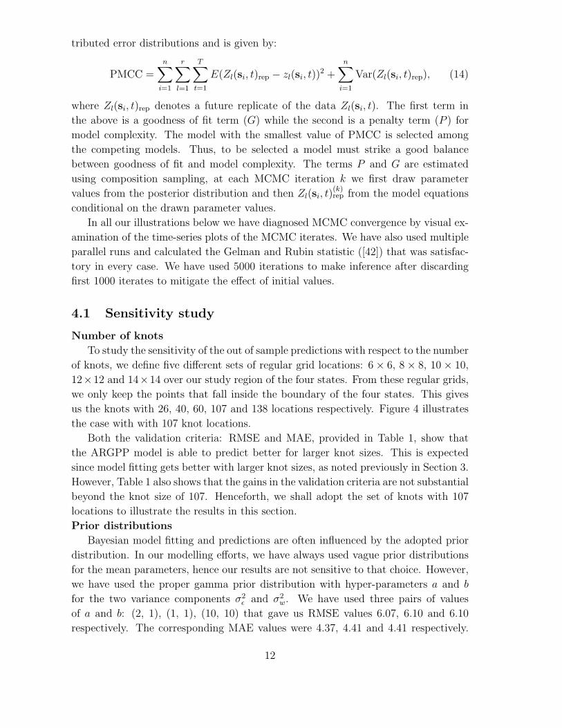
4.1 Sensitivity study
Number of knots
To study the sensitivity of the out of sample predictions with respect to the number
of knots, we define five different sets of regular grid locations: 6 × 6, 8 × 8, 10 × 10,
12×12 and 14×14 over our study region of the four states. From these regular grids,
we only keep the points that fall inside the boundary of the four states. This gives
us the knots with 26, 40, 60, 107 and 138 locations respectively. Figure 4 illustrates
the case with with 107 knot locations.
Both the validation criteria: RMSE and MAE, provided in Table 1, show that
the ARGPP model is able to predict better for larger knot sizes. This is expected
since model fitting gets better with larger knot sizes, as noted previously in Section 3.
However, Table 1 also shows that the gains in the validation criteria are not substantial
beyond the knot size of 107. Henceforth, we shall adopt the set of knots with 107
locations to illustrate the results in this section.
Prior distributions
Bayesian model fitting and predictions are often influenced by the adopted prior
distribution. In our modelling efforts, we have always used vague prior distributions
for the mean parameters, hence our results are not sensitive to that choice. However,
we have used the proper gamma prior distribution with hyper-parameters a and b
for the two variance components σ2ǫ and σ2
w. We have used three pairs of values
of a and b: (2, 1), (1, 1), (10, 10) that gave us RMSE values 6.07, 6.10 and 6.10
respectively. The corresponding MAE values were 4.37, 4.41 and 4.41 respectively.
12

Hence, the predictions are not very sensitive to the choice of hyperparameter values
and henceforth we adopt the pair of values 2 and 1 for a and b.
Sampling method for φ
The choice of the estimation method for the spatial decay parameter, φ, has an
effect on the prediction results. In a classical inference setting it is not possible to con-
sistently estimate both φ and σ2w in a typical model for spatial data with a covariance
function belonging to the Matern family, see [43]. Moreover, [13] shows that spatial
interpolation is sensitive to the product σ2wφ but not to either one individually. That
is why, [44] choose the decay parameter using an empirical Bayes (EB) approach by
minimising the RMSE and estimate the variance parameter σ2w conditionally on the
fixed estimated value of φ. Here we avoid the EB approach by sampling φ from its
full conditional distribution in two different ways corresponding to two different prior
distributions. The first of these is a discrete uniform prior distribution on 20 equally
spaced mass points in the interval (0.001, 0.1). Here, although time consuming, the
full conditional distribution is discrete and sampling is relatively straightforward, see
the appendix. The second strategy, corresponding to a continuous uniform prior dis-
tribution in the interval (0.001, 0.1) for φ, is the random walk Metropolis-Hastings
algorithm tuned to have an optimal acceptance rate between 20% to 40%, see the
appendix. In one of our implementations, we have been able to tune this algorithm
to achieve an acceptance rate of 32.4% that gave an RMSE value of 6.07. The RMSE
value for the discrete sampling method was 6.16. The respective MAE values were
4.37 and 4.46. Thus the Metropolis-Hastings method provides better validation re-
sults and henceforth this method is adopted.
Choice of hold-out data
Results may be sensitive to the particular hold-out data set. We study this as
follows. We randomly choose 10 different hold-out data sets, each of them consisting
of observations from 16 out of the 164 total monitoring sites in the study region of
four states. The RMSEs for these 7 hold-out data sets vary between 6.07 and 6.20
whereas the MAEs are between 4.36 and 4.55. This shows that the validation results
are not much sensitive to the choice of the hold-out data. Henceforth, we adopt
the original hold out data set that had the RMSE and MAE values 6.07 and 4.37,
respectively.
4.2 Comparison with the ARHIER model
This section is devoted to comparing the proposed ARGPP models with the ARHIER
models. Note that the ARGPP does not directly approximate ARHIER and hence the
latter is not likely to be uniformly better than the former, and hence this comparison
is meaningful. Both the models use the same three covariates, namely, maximum
temperature (MaxTemp), relative humidity (RH) and wind speed (WDSP). In both
the cases we also adopt the same prior distributions and use the Metropolis-Hastings
13

sampling algorithm for sampling the spatial decay parameters. In the GPP based
proposed model we use 107 knot points as decided above.
The estimates of the parameters of the two models are provided in Table 2, except
for the parameters µl and σ2l under the ARHIER model and σ2
l under the ARGPP
model, l = 1, . . . , r since those estimates are not interesting for model comparison pur-
poses. Both the models show significant effect of the three covariates, although the
effects get attenuated under the ARHIER model due to the presence of the temporal
auto-regression. Further discussion about these effects is provided in Section 5. How-
ever, there are large differences between the two models as regards to the estimates
of spatial and temporal correlations. The temporal correlation under the ARHIER
(0.523) is much larger than the same for the ARGPP model (0.092). This is due to the
fact that the auto-regressive model for the Sahu et al. version is assumed for the true
ozone levels which are highly temporally correlated, whereas the GPP based model
assumes the auto-regression for the latent random effects which are also significantly
temporally correlated but at a magnitude lower than that for the true ozone levels
in ARHIER. However, to compensate for this low value of temporal correlation, the
GPP based model has estimated a much higher level of spatial correlation since the
spatial decay of 0.0036 is much smaller for this model compared to the same, 0.012,
for the full hierarchical AR model. The estimates of the variance components, under
both the models, show that more variation is explained by the spatial effects than
the pure error.
The two models are compared using the PMCC and the two model validation
criteria: RMSE and MAE. We also report the nominal coverage of the 95% prediction
intervals for the out of sample validation data. These three validation statistics are
based on 21,008 (=24480–3472) daily observations as noted above. Model comparison
results presented in Table 3 almost uniformly give evidence in favour of the the
proposed GPP based models. Components of the PMCC show that the GPP based
model provides a much better fit than the ARHIER. Both the RMSE and MAE
are also better for the proposed model. However, the nominal coverage is slightly
smaller for the proposed method, but this is not much of a cause for concern since
both are close to 95%. The ARGPP model fitting requires about 2.24 hours of
computing time while the full ARHIER model takes about 7.86 hours. Thus the
ARGPP implementation requires less than a third of the computing time needed for
fitting the ARHIER model. In conclusion, the ARGPP model not only provides a
faster and better fit but also validates better than the ARHIER. In the next section,
for the full eastern US data, we shall only consider the GPP based model.
14

5 Analysis of the full eastern US data set
We now analyse the full eastern US data set introduced in Section 2. We use data from
622 monitoring sites to model and the data for the remaining 69 sites are set aside
for validation, see Figure 1. We continue to use the three meteorological variables
as covariates in the model. We choose the same prior and the Metropolis-Hastings
sampling method for the spatial decay parameter φ. To select the number of knots
we start with regular grid sizes of 12 × 12, 15 × 15, 20 × 20 and 25 × 25 and then
only retain the points inside the land boundary of the eastern US that gives us 68,
105, 156 and 269 points respectively. As in previous section we fit and predict using
the model with these knot sizes and obtain the two validation statistics: RMSE and
MAE in Table 4. As has already been seen in Section 4, the performance gets better
with increasing grid sizes, but the improvement in performance is only marginal when
the grid size goes up to 269 from 156. The much smaller computational burden with
156 knot points outweighs this marginal improvement in the validation statistics.
Henceforth we proceed with the grid size 156 in our analysis. Figure 5 provides a
map of the eastern US with these grid points superimposed.
Parameter estimates of the fitted model with 156 knot points are provided in
Table 5. All three covariates, MaxTemp, RH and WDSP, remain significant in the
spatio-temporal model with a positive effect of MaxTemp and negative effects of the
other two. This is in accordance with the results in the literature in ozone modelling,
see e.g., [4]. The auto-regressive parameter is also significant and the pure error
variance σ2ǫ is estimated to be smaller than the spatial variance σ2
w. The spatial
decay parameter is estimated to be 0.0018 which corresponds to an effective spatial
range ([54]) of 1666.7 kilometers that is about half of the maximum distance between
any two locations inside the study region. The estimates of σ2l for l = 1, . . . , r range
from 0.457 to 3.828 and are omitted for brevity.
We now turn to the validation of the ozone summaries: the annual 4th highest
maximum and the 3-year rolling average of these. Table 6 provides the validation
statistics. We also report the values of the validation statistics for these summaries
obtained using simple kriging using the fields package [35]. In this kriging method,
the daily ozone levels are first kriged and then those are aggregated up to the annual
levels to mimic our model based approach where we spatially predict on each day and
then aggregate the predictions up to the annual levels. As expected, the proposed
method is able to perform better in out of sample predictions than standard kriging
which is well known to be difficult to beat using model based approaches ([33]). This
shows that the model is very accurate in predicting the primary ozone standard based
on the annual summaries. Figure 6 examines this in more detail where the predicted
values of these summaries are plotted against the observed values. The plot provides
evidence of accurate prediction with a slight tendency to over-predict. The actual
over prediction percentage for the annual 4th highest maximum is 52% while the
15

same for the 3-year rolling averages is slightly higher at 53% which are reasonable.
Hence we proceed to make predictive inference for the ozone standard based on these
model based annual summaries.
We perform predictions at 936 locations inside the land-boundary of the eastern
US obtained from a regular grid. At each of these sites we spatially interpolate the
daily maximum 8-hour average ozone level on each of 153 days in every year using the
details in Section 3.3.2. These daily levels are then aggregated up to the annual levels.
Figure 7 provides the model based interpolated maps of annual 4th highest maximum
ozone levels for the years 1997-2006. Observed values of these annual maxima from a
selected number of sites (data from all the 691 sites are not plotted to avoid clutter)
are also superimposed and those show reasonably good agreement with the predicted
values. Similarly, Figure 8 plots the model based interpolated maps of the 3-year
rolling averages of the annual 4th highest maximum ozone concentration levels for
the years 1999-2006. The 3-year averages increase slightly or remain generally at
a constant level from 1999 to 2003 and then decrease. The superimposed observed
values of these rolling averages are also in good agreement with the predicted values.
The uncertainty maps corresponding to the prediction maps in Figures 7 and 8 showed
larger uncertainty for the locations which are farther away from the monitoring sites
and are omitted for brevity. The predicted maps show a gradually decreasing trend on
ozone levels that can be attributed to gradual reductions in ozone precursor emissions,
specially in nitrogen oxides and volatile organic compounds – the main ingredients
of ozone. We study the meteorologically adjusted relative percentage trends (see
Section 3.3.3) in Figure 9 for 2006 relative to 1997. We observe most of these trends
to be negative except for a few sites.
The model based predictive maps of the probability that the 3-year rolling average
of the annual 4th highest maximum ozone level is greater than 85 ppb, i.e. non-
compliance with respect to the primary ozone standard, are provided in Figure 10.
The plots show that many areas were out of compliance in the earlier years e.g. in
1999-2003. However, starting in 2004 most areas started to comply with the primary
ozone standard and except for few areas shown in the maps. As mentioned above
this can be attributed to emission reduction policies adopted be many federal and
local government agencies. Another noticeable feature of the Figures 7 and 10 is that
the spatial patterns in the successive years maps change relatively slowly. This is
also expected as the annual 4th highest ozone levels and the 3-year rolling averages
of the annual 4th highest ozone levels change very gradually, see Figure 3 where the
observed values of these have been plotted.
16

6 Relevance to business and industry
The hierarchical modeling methods developed in this paper allow accurate modeling
of localized spatial variation that may change over time. This in turn enables accurate
spatial prediction and inference at the highest spatial resolution at the point-level.
The general spatio-temporal modeling methods are widely applicable in any suitable
industrial example settings. For example, consider the industrial corrosion problem
where it is important to know the extent of corrosion at any particular location as
discussed in [46]. Corrosion is a common industrial problem that affects furnaces,
pipelines, storage tanks, valves, nozzles and many other systems in the oil and other
industries. The proposed dynamic space-time models enable early identification of
corrosion that may result in the initiation of preventative measures and accurate
forecasting of such events in the future. A concrete modeling example is outlined
below.
Consider the modeling of corrosion in a large industrial furnace as described in [46].
Health and safety concerns require inspection of the furnace at regular time intervals
and recording of the vessel wall thickness at a large number of sites in the furnace.
According to past experience of the experts, it is reasonable to assume that the wall
thickness will, on average, deteriorate continuously if operating conditions remain
constant, and that current corrosion rate is the best estimator of the future corrosion
rate. Therefore, the wall thickness is modeled with a locally linear trend as in (4)
with details modified as follows.
Let Z(s, t) denote the observed wall thickness value at a location s and time t.
We drop the subscript l since time here can be described by just one index t. We also
suppose that there are observed covariates, denoted by xl(s, t), that may help explain
corrosion in the wall thickness. For example, components of xl(s, t) may record the
furnace usage history in the period before time t, and/or an exposure characteristics
at location s at time t such as temperature. As in previous section we introduce two
sets of independent error distributions: one spatial, denoted by η(s, t), and the other
a measurement error, ǫ(s, t). As in (4) we can now write the model as:
Z(s, t) = x′(s, t)β(s) + η(s, t) + ǫ(s, t).
In this model β(s) are unknown spatially varying regression co-efficients that can
be estimated from the data. If, however, there are no measurable covariates present
then we can simply assume the time invariant intercept process β0(s) that signifies
the overall thickness that will remain even after the end of the life of the vessel. A
zero mean Gaussian process prior, see for example, [54] can be assumed for the β0(s)
process.
A suitable dynamic model must be assumed for the spatially correlated error
process η(s, t). Following the development in this paper we assume an auto-regressive
model as given in (5). This model for the spatial residuals is intuitively sensible
17

here because of the above assumption that the wall thickness deteriorates on average
under constant operating conditions. This also justifies the auto-regressive models
proposed here instead of the random-walk models, see for example, [54]. The drift
term, x′(s, t)β(s), in the overall model can be used to accommodate any effects of
change in these conditions. The remaining model and prior distributions are assumed
to be the same as in Section 3. The problem of handling large spatial and spatio-
temporal industrial data, such as the wall thickness data, can be alleviated by the
GPP based modeling developments of this paper. Many specific implementation
parameters such as the knot size need to be chosen from a suitable sensitivity study.
The Bayesian spatio-temporal models can potentially solve a very important prac-
tical forecasting problem as follows. Often, it is of interest to assess the probability
that the wall thickness, Z(s′, t), at any location s′ at any future time point t is less
than a given threshold design value. These types of failure probabilities can be easily
estimated by the methods developed in Sections 3.3.2 and 3.3.4. Moreover, these
probabilities can be plotted on a map that can be continuously updated once new
data become available.
The model validation methods by using hold-out data provide automatic ways of
checking the full model and its assumptions. These out of sample validation statistics
can also be used to compare all the competing modeling strategies discussed in this
paper since the one of the main objectives of the modeling exercise here is to obtain
out of sample predictions and forecasts.
The discussion here points to the possibility that future investigations with real
data sets are likely to lead to fruitful results especially relevant to businesses and
industries. However, as is well known, the take-up of the stochastic models by the
businesses often does not proceed at a desirable fast pace due to the lack of availabil-
ity of suitable software packages that implement the methods. This is where the R
package spTimer that has been developed alongside this paper and is freely available
can help. This package can do the model fitting, prediction and forecasting for large
space-time data sets.
Lastly, we note that the substantive environmental modeling example of this pa-
per is also of direct relevance to many businesses and industries. For example, the
accurate spatial prediction of the long term trends in air pollution is likely to influ-
ence current and future emission reduction policies. These policies will directly affect
the method and the cost of industrial production which will have long-term repercus-
sions in the local economy. Further general discussions of the developed methods are
provided in the next section.
18

7 Discussion
A fast hierarchical Bayesian auto-regressive model for both spatially and temporally
rich data sets has been developed in this paper. The methods have been shown to be
accurate and feasible for simultaneous modelling and analysis of a large data set with
more than a million observations using computationally intensive MCMC sampling
algorithms. The proposed auto-regressive models have been shown to validate better
than standard Kriging for out of sample predictions.
Specifically, the methods have been illustrated for evaluating meteorologically
adjusted trends in the primary ozone standard in the eastern US over a 10 year
period from 1997-2006. To our knowledge no such Bayesian model based analysis
exists for the same data and the same modelling purposes. An important utility of
the high resolution space-time model lies in the ability to predict the primary ozone
standard at any given location for the modelled period. This helps in understanding
spatial patterns and trends in ozone levels both at the meteorologically adjusted and
unadjusted levels which in turn will help in evaluating emission reduction policies
that directly affect many industries.
The proposed methods can also be used in conjunction with a spatio-temporal
downscaler model for incorporating output from numerical models as discussed in
[47] and [48]. The essence of the down-scaler model is to use the grid-level output
from numerical models as a covariate in the point level model such as (4). This type
of space and time varying covariate information enriches the regression settings like
the one in the ARGPP model (8) and in fact will allow us to estimate spatially and/or
temporally varying regression coefficients ([49] and [47]) in the model, see also [50]. A
downscaler model with or without our ARGPP approach, however, cannot be used for
assessing meteorologically adjusted trends since the outputs of the numerical models
are based on the meteorological data and including the meteorological data again in
the model will lead to multi-collinearity problems.
An R package, spTimer, has been developed for implementing the models for
analysing large volumes of space-time data and will be made publicly available from
the R archive network CRAN (http://cran.r-project.org/). The spTimer package with
its ability to fit, predict and forecast using a number of space-time models can be
used for modelling a wide variety of large space-time data.
Multivariate space-time modelling for large data sets is a challenging task. The
methods developed in this paper can be extended to cope with a multivariate space-
time random effect that can be specified using a linear model of coregionalisation, see
e.g., [51]. An alternative of this last method is to specify the multivariate response
conditionally, see e.g., [52] where ozone concentration levels and particulate matter
data have been modelled jointly.
19
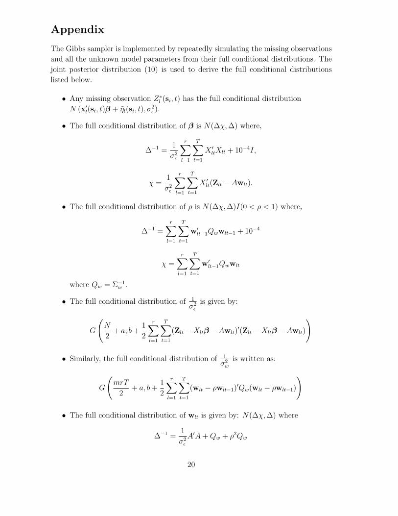
Appendix
The Gibbs sampler is implemented by repeatedly simulating the missing observations
and all the unknown model parameters from their full conditional distributions. The
joint posterior distribution (10) is used to derive the full conditional distributions
listed below.
• Any missing observation Z∗
l (si, t) has the full conditional distribution
N (x′
l(si, t)β + ηl(si, t), σ2ǫ ).
• The full conditional distribution of β is N(∆χ,∆) where,
∆−1 =1
σ2ǫ
r∑
l=1
T∑
t=1
X ′
ltXlt + 10−4I,
χ =1
σ2ǫ
r∑
l=1
T∑
t=1
X ′
lt(Zlt − Awlt).
• The full conditional distribution of ρ is N(∆χ,∆)I(0 < ρ < 1) where,
∆−1 =r∑
l=1
T∑
t=1
w′
lt−1Qwwlt−1 + 10−4
χ =r∑
l=1
T∑
t=1
w′
lt−1Qwwlt
where Qw = Σ−1w .
• The full conditional distribution of 1
σ2ǫ
is given by:
G
(
N
2+ a, b+
1
2
r∑
l=1
T∑
t=1
(Zlt −Xltβ − Awlt)′(Zlt −Xltβ − Awlt)
)
• Similarly, the full conditional distribution of 1
σ2w
is written as:
G
(
mrT
2+ a, b+
1
2
r∑
l=1
T∑
t=1
(wlt − ρwlt−1)′Qw(wlt − ρwlt−1)
)
• The full conditional distribution of wlt is given by: N(∆χ,∆) where
∆−1 =1
σ2ǫ
A′A+Qw + ρ2Qw
20
χ =1
σ2ǫ
A′(Zlt −Xltβ) +Qwwlt−1 +Qwwlt+1,
for 1 ≤ t < T . For t = T , we have
∆−1 =1
σ2ǫ
A′A+Qw
χ =1
σ2ǫ
A′(Zlt −Xltβ) +Qwwlt−1.
• The full conditional distribution of wl0 is given by N(∆χ,∆) where,
∆−1 = ρ2Qw +Q−10
χ = ρQwwl1 + µlΣ−10 1m,
where Q0 = Σ−10 .
• The full conditional distribution of σ2l for l = 1, . . . , r is given by:
G
(
m
2+ a, b+
1
2wl0S
−10 wl0
)
.
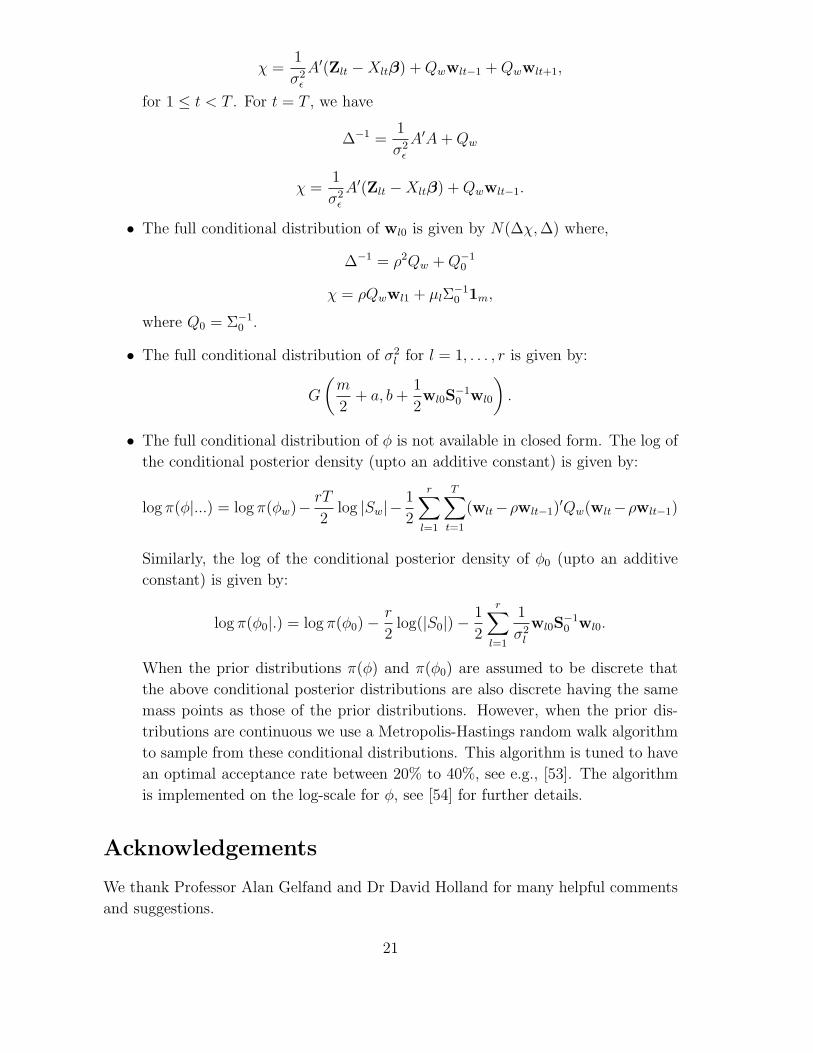
• The full conditional distribution of φ is not available in closed form. The log of
the conditional posterior density (upto an additive constant) is given by:
log π(φ|...) = log π(φw)−rT
2log |Sw|−
1
2
r∑
l=1
T∑
t=1
(wlt−ρwlt−1)′Qw(wlt−ρwlt−1)
Similarly, the log of the conditional posterior density of φ0 (upto an additive
constant) is given by:
log π(φ0|.) = log π(φ0) −r
2log(|S0|) −
1
2
r∑
l=1
1
σ2l
wl0S−10 wl0.
When the prior distributions π(φ) and π(φ0) are assumed to be discrete that
the above conditional posterior distributions are also discrete having the same
mass points as those of the prior distributions. However, when the prior dis-
tributions are continuous we use a Metropolis-Hastings random walk algorithm
to sample from these conditional distributions. This algorithm is tuned to have
an optimal acceptance rate between 20% to 40%, see e.g., [53]. The algorithm
is implemented on the log-scale for φ, see [54] for further details.
Acknowledgements
We thank Professor Alan Gelfand and Dr David Holland for many helpful comments
and suggestions.
21

References
[1] Banerjee, S., Gelfand, A.E., Finley, A.O. & Sang, H. (2008). Gaussian Predic-
tive Process Models for Large Spatial Data Sets. Journal of the Royal Statistical
Society, Series: B, 70, 825-848.
[2] Franklin, C. (1992). An introduction to geographic information systems: linking
maps to databases. Database, 15, 13-21.
[3] Cressie, N. and Wikle, C. K. (2011) Statistics for Spatio-Temporal Data. John
Wiley & Sons.
[4] Sahu, S. K., Gelfand, A. E. and Holland, D. M. (2007). High Resolution Space-
Time Ozone Modeling for Assessing Trends. Journal of the American Statistical
Association, 102, 1221-1234.
[5] Cameletti, M., Ignaccolo, R. and Bande, S. (2009). Comparing Air Quality
Statistical Models. Technical Report. University of Bergamo, Italy.
[6] Sahu, S. K. and Bakar, K. S. (2011) A comparison of Bayesian Mod-
els for Daily Ozone Concentration Levels Statistical Methodology, DOI:
10.1016/j.stamet.2011.04.009.
[7] Banerjee, S., Carlin, B.P. and Gelfand, A.E. (2004). Hierarchical Modeling and
Analysis for Spatial Data. Chapman and Hall/CRC.
[8] Cressie, N.A.C (1993). Statistics for Spatial Data. John Wiley and Sons, New
York, revised edition.
[9] Haas, T.C. (1995). Local prediction of a spatio-temporal process with an appli-
cation to wet sulfate deposition. Journal of the American Statistical Association,
90, 1189-1199.
[10] Kammann, E.E. & Wand, M.P. (2003). Geoadditive models. Applied Statistics,
52, 1-18.
[11] Xia, G. and Gelfand, A.E. (2006). Stationary Process Approximation for the
Analysis of Large Spatial Datasets. Technical Report. Institute of Statistical and
Decision Sciences, Duke University, Durham, USA.
[12] Nychka, D. (2000). Spatial-process estimates as smoothers. In Smoothing and
Regression: Approaches, Computation, and Application. Eds. M.G. Schimek,
393-424, New York, Wiley.
[13] Stein, M.L. (1999). Statistical Interpolation of Spatial Data: Some Theory for
Kriging. New York: Springer.
22

[14] Paciorek, C.J. (2007). Computational techniques for spatial logistic regression
with large datasets. Computational Statistics and Data Analysis, 51, 3631-3653.
[15] Hartman, L. and Hossjer, O. (2008) Fast kriging of large data sets with Gaussian
Markov random fields. Computational Statistics & Data Analysis, 2331-2349.
[16] Rue, H. and Held, L. (2006). Gaussian Markov Random Fields: Theory and
Applications. Boca Raton: Chapman and Hall/CRC.
[17] Reich, B.J., Fuentes, M. and Dunson, D.B. (2011). Bayesian Spatial Quan-
tile Regression. Journal of the American Statistical Association, 106, DOI:
10.1198/jasa.2010.ap09237.
[18] Huang, H.C., Cressie, N. and Gabrosek, J. (2002). Fast, resolution-consistent
spatial prediction of global processes from satellite data. Journal of Computa-
tional and Graphical Statistics, 11, 63-88.
[19] Johannesson, G. and Cressie, N. (2004). Finding large-scale spatial trends in
massive, global, environmental datasets. Environmetrics, 15, 1-44.
[20] Johannesson, G., Cressie, N. and Huang, H.C. (2007). Dynamic multi-resolution
spatial models. Environmental and Ecological Statistics, 14, 5-25.
[21] Stein, M.L. (2007). Spatial variation of total column ozone on a global scale.
Annals of Applied Statistics, 1, 191-210.
[22] Stein, M.L. (2008). A modelling approach for large spatial datasets. Journal of
the Korian Statistical Society, 37, 3-10.
[23] Cressie, N.A.C & Johannesson, G. (2008). Fixed rank kriging for very large
spatial data sets. Journal of the Royal Statistical Society, Series: B, 70, 209-
226.
[24] Cressie, N., Shi, T., Kang, E. L. (2010). Fixed Rank Filtering for Spatio-
Temporal Data. Journal of Computational and Graphical Statistics, 19, 724-
745.
[25] Carroll, R. J., Chen, R., George, E. I., Li, T.H., Newton, H.J., Schmiediche, H.
and Wang, N. (1997). Ozone exposure and population density in Harris County,
Texas. Journal of the American Statistical Association, 92, 392-404.
[26] Guttorp, P., Meiring, W. and Sampson, P. D. (1994). A Space-time Analysis of
Ground-level Ozone Data. Environmetrics, 5, 241-254.
[27] Huang, L. S. and Smith, R. L. (1999). Meteorologically-dependent trends in
urban ozone. Environmetrics, 10, 103–118.
23

[28] Thompson, M. L., Reynolds, J., Cox, L. H., Guttorp, P., and Sampson, P. D.
(2001). A review of statistical methods for the meteorological adjustment of
tropospheric ozone. Atmospheric Environment, 35, 617-630.
[29] Huerta, G., Sanso, B., and Stroud, J. R. (2004). A spatiotemporal model for
Mexico City ozone levels. Journal of the Royal Statistical Society, Series C, 53,
231–248.
[30] Gilleland, E. and Nychka, D. (2005). Statistical Models for Monitoring and
Regulating Ground Level Ozone. Environmetrics, 16, 535-546.
[31] McMillan, N., Bortnick, S. M., Irwin, M. E. and Berliner, M. (2005). A hierar-
chical Bayesian model to estimate and forecast ozone through space and time.
Atmospheric Environment, 39, 1373–1382.
[32] Cocchi, D., Fabrizi, E., and Trivisano, C. (2005). A stratified model for the
assessment of meteorologically adjusted trends of surface ozone. Environmental
and Ecological Statistics 12, 1195-1208.
[33] Liu, Z., Le, N. D., Zidek, J. V. (2011) An empirical assessment of Bayesian
melding for mapping ozone pollution. Environmetrics, 22, 340-353.
[34] McMillan, N., Holland, D. M., and Morara, M., and Feng, J. (2010). Com-
bining numerical model output and particulate data using Bayesian space-time
modeling. Environmetrics, 21, 48-65.
[35] Fields Development Team (2006). fields: Tools for Spatial
Data. National Center for Atmospheric Research, Boulder, CO.
http://www.cgd.ucar.edu/Software/Fields.
[36] Bakar, K. S. (2011). Bayesian Analysis of Daily Maximum Ozone Levels. PhD
Thesis, University of Southampton. UK.
[37] Christos, P. (2011). Bayesian Spatial-Temporal Modelling of Air Pollution. PhD
Thesis. Bath University, UK.
[38] Bakar, K. S., Awang, N. and Sahu, S. K. (2011) Forecasting next day ozone
levels using Gaussian Predictive Processes. Under Preparation.
[39] Finley, A.O., S. Banerjee, and B.P. Carlin. (2007). spBayes: A program for
multivariate point-referenced spatial modeling. Journal of Statistical Software,
19:4.
[40] Bakar, K. S. and Sahu, S. K. (2011) spTimer: Spatio-Temporal Bayesian Mod-
elling using R. Under Preparation.
24

[41] Gelfand, A. E. and Ghosh, S. K. (1998). Model Choice: A Minimum Posterior
Predictive Loss Approach. Biometrika, 85, 1–11.
[42] Gelman, A. and Rubin, D.B. (1992). Inference from iterative simulation using
multiple sequences (with discussion). Statistical Science, 7, 457-511.
[43] Inconsistent estimation and asymptotically equal interpolations in model-based
geostatistics. Journal of the American Statistical Association, 99, 250–261.
[44] Sahu, S. K., Gelfand, A. E. and Holland, D. M. (2010). Fusing point and areal
level space-time data with application to wet deposition. Journal of the Royal
Statistical Society, C, 59, 77-103.
[45] Finley, A.O., Sang, H., Banerjee, S., and Gelfand, A. (2009). Improving the
performance of predictive process modeling for large datasets. Computational
Statistics and Data Anlaysis, 53, 2873-2884.
[46] Little, J., Goldstein, M., Jonathan, P. and den Heijer K. (2004). Spatio-
temporal modelling of corrosion in an industrial furnace. Appl. Stochastic Mod-
els Bus. Ind., 20, 219238.
[47] Berrocal, V. J., Gelfand, A. E. and Holland, D. M. (2010). A Spatio-Temporal
Downscaler for Output From Numerical Models. Journal of the Agricultural,
Biological and Environmental Statistics, 15, 176-197.
[48] Sahu, S. K., Yip, S. and Holland, D. M. (2009). Improved space-time forecasting
of next day ozone concentrations in the eastern US. Atmospheric Environment,
doi:10.1016/j.atmosenv.2008.10.028.
[49] Gelfand, A. E., Kim, H. J., Sirmans, C. F., and Banerjee, S. (2003). Spatial
modeling with spatially varying coefficient processes. Journal of the American
Statistical Association, 98, 387-396.
[50] Nobre, A. A., Sanso, B., and Schmidt, A. M. (2011) Spatially Varying Autore-
gressive Processes. Technometrics, 53, 310-321.
[51] Gelfand, A. E. Schmidt, A. M. Banerjee, S. and Sirmans, C. F. (2004). Nonsta-
tionary Multivariate Process Modelling through Spatially Varying Coregional-
ization (with discussion). Test, 2, 1–50.
[52] Daniels, M.J., Zhou, Z. G., and Zou, H. (2006) Conditionally specified space-
time models for multivariate processes. Journal of Computational and Graphical
Statistics, 15, 157-177.
25

[53] Gelman, A., Roberts, G. O., and Gilks, W. R. (1996). Efficient Metropolis
Jumping Rules. In Bayesian Statistics 5, edited by J. M. Bernardo, J. O. Berger,
A. P. Dawid and A. F. M. Smith. Oxford University Press, pp 599-607.
[54] Sahu, S. K. (2011). Hierarchical Bayesian models for space-time air pollution
data In Handbook of Statistics-Vol 30. Time Series Analysis, Methods and
Applications. Editors: T Subba Rao and C R Rao. Elsevier Publishers, Holland.
To appear.
Knot size 26 40 60 107 138
RMSE 6.31 6.19 6.17 6.07 6.06
MAE 4.58 4.48 4.44 4.37 4.36
Table 1: Values of the two validation criteria for different knot sizes for the four states
example.
Parameter Mean SD 2.5% 97.5%
ARHIER
Intercept 4.447 0.061 4.346 4.541
Max.Temp. 0.016 0.001 0.013 0.018
RH –0.314 0.010 –0.325 –0.302
WDSP –0.061 0.002 –0.065 –0.057
ρ 0.523 0.002 0.519 0.526
σ2ǫ 0.056 0.001 0.055 0.058
σ2η 0.537 0.038 0.527 0.540
φ 0.0120 0.0006 0.0119 0.0121
ARGPP
Intercept 6.353 0.056 6.224 6.445
MaxTemp 0.060 0.001 0.057 0.063
RH –0.179 0.009 –0.198 –0.160
WDSP –0.033 0.001 –0.036 –0.031
ρ 0.102 0.003 0.095 0.109
σ2ǫ 0.169 0.001 0.167 0.171
σ2w 0.457 0.004 0.449 0.466
φ 0.0036 0.0001 0.0030 0.0041
Table 2: Parameter estimates of the two AR models.
26
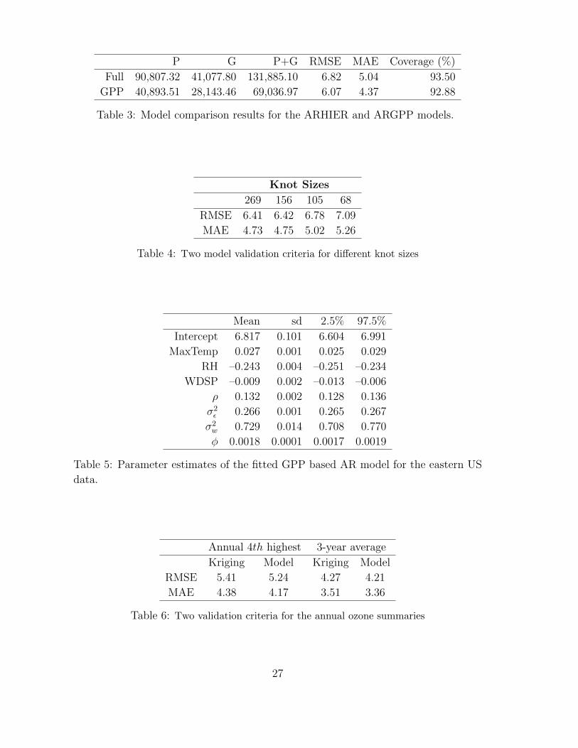
P G P+G RMSE MAE Coverage (%)
Full 90,807.32 41,077.80 131,885.10 6.82 5.04 93.50
GPP 40,893.51 28,143.46 69,036.97 6.07 4.37 92.88
Table 3: Model comparison results for the ARHIER and ARGPP models.
Knot Sizes
269 156 105 68
RMSE 6.41 6.42 6.78 7.09
MAE 4.73 4.75 5.02 5.26
Table 4: Two model validation criteria for different knot sizes
Mean sd 2.5% 97.5%
Intercept 6.817 0.101 6.604 6.991
MaxTemp 0.027 0.001 0.025 0.029
RH –0.243 0.004 –0.251 –0.234
WDSP –0.009 0.002 –0.013 –0.006
ρ 0.132 0.002 0.128 0.136
σ2ǫ 0.266 0.001 0.265 0.267
σ2w 0.729 0.014 0.708 0.770
φ 0.0018 0.0001 0.0017 0.0019
Table 5: Parameter estimates of the fitted GPP based AR model for the eastern US
data.
Annual 4th highest 3-year average
Kriging Model Kriging Model
RMSE 5.41 5.24 4.27 4.21
MAE 4.38 4.17 3.51 3.36
Table 6: Two validation criteria for the annual ozone summaries
27

NAMS/SLAMS sitesCASTNET sitesValidation sitesMeteorological sites
Figure 1: A map showing the locations of the ozone concentration and weather mon-
itoring sites.
050
100
150
200
250
Dai
ly m
axim
um 8
-hou
r oz
one
1997 1998 1999 2000 2001 2002 2003 2004 2005 2006
Year
Figure 2: Boxplot of daily maximum eight-hour ozone concentration levels by years.
28

Years
Annual
4th high
est max
imum o
zone
1997 1999 2001 2003 2005
050
100150
200
Years
Three y
ear roll
ing ave
rage
1999 2000 2001 2002 2003 2004 2005 2006
6080
100120
140
Figure 3: Time series plots of the ozone concentration summaries from 691 sites: (a)
annual 4th highest maximum and (b) 3-year rolling average of the annual 4th highest
maximum.
Fitted sitesValidation sitesMeteorological sitesKnot points
Figure 4: A map of the four states: Illinois, Indiana, Ohio, and Kentucky show-
ing 164 ozone monitoring sites consisting of 148 fitting and 16 validation sites, 88
meteorological sites and 107 knot locations.
29

Figure 5: A map of the eastern US with 156 knot points superimposed.
*
*
*
*
*
*
*
*
*
*
**
*
*
*
*
*
*
*
*
**
*
*
*
*
*
*
**
*
*
*
*
*
*
*
***
*
*
** *
***
*
*
*
*
*
*
*
*
*
**
*
*
*
*
*
*
*
*
*
*
*
*
*
*
*
*
*
*
*
*
*
* *
*
*
*
*
*
*
*
*
**
*
*
*
*
*
*
*
*
**
*
*
*
*
*
*
*
*
* *
*
*
*
*
*
*
**
**
*
*
*
*
*
*
**
*
*
*
*
*
*
*
*
* *
*
*
*
*
*
*
*
*
*
*
*
*
*
*
*
*
*
*
*
*
*
*
*
*
*
*
*
*
**
**
*
*
*
*
*
*
*
*
*
*
*
*
*
*
*
**
*
*
*
*
*
*
*
*
**
*
*
*
*
*
*
* *
*
*
*
*
*
**
*
*
*
*
*
*
**
**
**
*
*
*
*
*
*
*
*
*
*
*
*
*
*
*
*
*
*
*
*
*
*
*
*
*
*
*
*
**
*
*
*
*
*
*
*
*
*
*
*
*
*
*
*
*
*
*
*
*
*
*
*
*
*
*
*
*
*
*
*
**
*
*
*
*
*
**
*
**
**
*
*
*
*
*
*
**
*
*
*
*
*
**
*
* *
* *
*
*
*
**
*
**
**
*
*
*
*
*
*
**
**
*
*
*
*
*
*
**
*
*
*
*
*
*
*
*
**
*
*
*
*
*
*
*
*
**
*
*
*
*
*
*
*
*
*
*
*
*
*
*
*
*
*
*
*
*
*
*
*
*
*
*
*
*
*
*
*
*
*
*
*
*
*
**
*
*
*
*
*
*
*
*
*
**
*
*
*
*
*
*
*
*
*
*
*
*
*
*
*
*
*
*
*
*
*
*
*
*
* **
*
*
*
*
*
*
*
*
*
*
*
*
*
*
*
*
**
*
*
*
*
*
*
*
*
*
*
*
**
*
*
*
*
*
*
*
**
*
**
*
*
*
*
*
*
*
*
*
*
*
*
*
*
*
*
*
*
*
*
*
*
*
*
*
*
**
*
*
*
*
*
**
*
***
*
***
*
*
*
*
*
*
*
*
**
*
*
*
*
*
*
*
**
**
*
*
*
*
*
*
*
**
*
*
*
*
*
*
* *
** *
*
*
*
*
*
*
*
*
*
*
*
* *
**
*
*
*
*
*
*
*
*
*
*
*
*
*
*
*
*
*
*
*
*
*
*
*
*
**
*
*
*
*
*
*
*
*
*
*
*
*
*
*
*
*
*
**
*
*
*
*
*
*
*
*
*
*
*
*
60 70 80 90 100
6070
8090
100
Observed
Pred
icted
(a)
*
*
*
**
*
*
*
*
*
*
**
*
**
*
***
*
*
**
**
*
**
*
*
*
**
*
*
*
**
*
*
*
*
*
*
*
*
*
*
**
*
*
*
*
*
*
**
*
*
**
*
**
*
*
*
**
**
*
*
*
*
**
*
**
*
*
*
**
*
*
*
*
**
**
**
*
*
**
**
*
**
*
*
*
*
*
*
**
*
*
*
*
**
*
*
*
*
*
*
**
*
*
*
*
*
**
***
*
*
** ***
*
**
**
**
*
*
**
**
**
*
*
**
*
*
*
*
* *
**
*
*
*
*
* *
**
*
***
*
*
* *
*
*
*
*
*
*
*
*
*
*
*
*
*
*
**
*
***
*
*
*
*
*
*
*
**
*
*
*
*
*
*
*
*
*
*
*
*
*
**
*
*
**
**
*
*
*
*
*
*
**
*
*
*
*
*
*
*
*
**
*
*
*
*
**
**
*
*
*
*
**
**
*
*
*
*
**
*
**
*
*
*
**
*
* *
*
*
*
**
*
*
*
*
*
*
**
*
**
*
*
*
**
*
* *
*
*
*
**
*
**
*
*
*
*
* *
**
*
*
*
***
**
*
*
*
**
*
* *
*
*
*
**
*
**
*
*
**
**
*
**
*
*
*
*
*
*
**
*
*
*
*
*
*
* *
*
*
* **
*
* *
*
*
***
*
*
*
***
*
*
* *
*
**
**
*
*
*
*
*
*
**
*
*
**
*
*
*
*
**
*
***
*
*
* *
*
**
*
*
**
*
**
*
*
**
*
*
**
*
**
*
***
*
*
*
*
*
*
*
***
* *
*
**
*
*
*
*
*
*
*
*
*
*
*
*
*
**
*
*
*
*
*
*
*
*
*
*
*
*
*
*
*
*
*
*
*
*
*
60 70 80 90 100
6070
8090
100
Observed
Pred
icted
(b)
Figure 6: Scatter plots of the prediction against the observed values, (a): annual 4th
highest maximum, (b) 3-year rolling average of the annual 4th highest maximum.
The y = x line is superimposed.
30

70
75
80
85
90
95
100
79
81.9
62
91.968.576.1
105.5
9990.1
68.9
63.2
81.9
69.8
78.6
89.9
87 87.2
68.6 76.9
82.5
74.2
82.5
86
97.5
95.9
66.963.1
63.7
77.863.8
88.478
74.4
76.4
100.2
82
82.2
72.5
63
79.2
95.9
61.5
73
73.6
79.6
80.974.6
84.495.4
90.4
87.2
73.1
64.5
69
68.4
(a)
70
75
80
85
90
95
100
105
94
98.1
68.5
86.171.874.8
92
10298.8
93.1
76.4
97.9
85.2
88.1
96.4
98.2 99.8
73.6 83.9
78.9
76.2
91.6
89.7
103.5
100.5
79.466.5
68.4
48.5
86.585.4
91.582.5
84.5
77.6
84.4
90.2
89.9
72.5
64.8
82.5
91.9
71.5
82.2
94.2
79.5
96.595.8
79.896.4
96.5
103.4
77
76.1
77.5
62.5
88.2
83.6
(b)
75
80
85
90
95
100
105
91
85.6
73.8
96.173 77.1
106.2
97.897.1
75.4
69.6
86.1
76.8
81.6
103
102.5 90.5
75.2 94.2
80.5
80.9
100.1
90.5
89.6
96.6
68.876.9
74
58.5
9881
88.880.1
83.1
80.9
101.5
97.5
89.5
73.8
68.6
82.1
84.2
74.8
82.1
90.1
84.2
82.284.6
9191.5
90
94.6
85.8
86.6
84.2
65.6
94.9
83.889.2
(c)
65
70
75
80
85
90
95
100
77.2
88.5
80
91.971.188.3
90.1
93.994.2
75.9
55.5
82.9
76.4
80.1
97.5
98 90.8
71 68.8
67.6
80.4
83.2
91.6
85.2
90
75.272.6
71.4
61.4
82.578.4
98.981.1
80.6
63.6
83
81
72.5
66.3
61.4
80.5
84.4
78
73.8
85.1
82.2
91.590.4
71.192.6
82.4
95.2
72.6
65.6
73.1
59.4
84.8
79.282.5
93.6
(d)
70
75
80
85
90
95
100
83.2
75.8
72.6
92.262.1 78
96
91.488.8
79
72.2
83.6
67.9
78.1
86.2
85.4 81.6
78 73.2
77.8
71.9
84.9
82.6
86.9
88.8
78.269.9
63.8
58
71.675.8
75.271.9
74.4
84.1
105.8
91.6
91.2
73.7
57.2
77.8
73.8
69.5
82
102.4
85.6
88.676.9
79.687.2
97.2
87.9
88
75.5
69.1
68.2
79.9
70.974.9
84.4
(e)
60
70
80
90
100
83
75
78.8
10074.182.5
109
94.597.8
69.4
49.9
71.1
70.1
75.9
93.5
95.6 91.4
82 82.8
94.1
89.8
100.2
93.8
100.8
101.1
78.170.1
65.2
59.6
92.882.2
75.570.1
73.4
88.1
93.2
86.1
88.2
71.8
64.8
72.1
83.5
78.9
89
105
94.1
95.990.8
95
103.9
94.2
84
66.8
73.2
68.4
80.8
74.174.8
76.5
(f)
60
70
80
90
71.6
71.5
64.1
84.858.971.2
85.2
8479.9
68.6
50.8
78.2
67.6
74.4
80.5
83.8 74
71.4 75.6
77.2
77.5
83.6
90.4
90
101
73.268
63.2
51.1
72.162.7
74.877.2
70
69.8
89.6
89.1
87.1
71.1
59.4
65.5
85.2
67.4
73.8
92.8
95.6
81.570.9
82.183.1
99.5
82.8
77.1
68.5
74
58.1
72.2
69.568
77.4
(g)
60
65
70
75
80
85
71.6
74.8
59.9
78.659.972.4
86
75.480.5
75.5
51.1
77.1
69.8
76.8
86.1
84.8 80.6
63.2 62
65.5
70
73.9
69.2
74.6
75.8
71.264
58.6
58.9
62.260
82.574.8
75.8
70
83
75.1
75
62.9
55.6
67
67.4
62
77.2
79.4
69.966.1
72.170.9
81.9
70.6
60.9
64.1
61.1
68.5
7171.2
70.6
(h)
65
70
75
80
85
90
71.6
70.8
60.9
96.586.5
104.4
81.277.9
67.5
59.4
76.9
68.2
84.6
82
87 80.9
76.1 73.4
84.8
86.4
86.9
80.4
87.8
80.173.5
62.5
72.5
69.4
80.868.9
69.2
70.6
87.9
86.8
77.3
77.1
66.1
74.9
79.6
69.8
90
78.4
72.672.8
93.2
79.9
70.1
73.5
57.4
76.6
67.474.4
82
(i)
65
70
75
80
85
90
74.1
85.5
67.6
89.878.8
87.9
85.483.4
72.2
70.6
76.8
73
77.9
77.2
96.1 83.1
71.1 64.4
78.4
75.8
73.9
79.6
77.6
7563.9
59.6
69.8
63.1
88
65
82
80.6
72.5
72.6
63
78.5
91.4
67.2
83.8
71.6
67.975.4
86.8
66.1
65.2
66.8
60
76.2
63.579.2
82.9
(j)
Figure 7: Model based interpolation of the annual 4th highest maximum ozone levels
for 10 years, panel (a) for 1997 to panel (j) for 2006. Observed data from a few
selected sites, to enhance readability, are superimposed.
31

75
80
85
90
95
100
105
88
88.5
68.1
91.471.1 76
101.2
99.695.3
79.1
69.8
88.6
77.2
82.8
96.4
95.9 92.5
72.5 85
80.6
77.1
91.4
88.7
96.9
97.7
71.768.8
56.9
87.476.7
89.680.2
80.7
78.3
95.4
89.9
87.2
72.9
65.5
81.3
90.7
69.2
79.1
86
81.1
86.585
8594.4
92.3
95.1
78.6
75.8
76.9
65.5
(a)
70
75
80
85
90
95
100
87.4
90.8
74.1
91.472 80.1
96.1
97.996.7
81.5
67.2
89
79.5
83.3
99
99.6 93.7
73.3 82.3
75.7
79.2
91.7
90.6
92.8
95.7
74.572
71.3
56.1
8981.6
93.181.3
82.7
74
89.6
89.6
84
70.8
64.9
81.7
86.8
74.8
79.4
89.8
82
90.190.3
80.693.5
89.6
97.8
78.5
76.1
78.3
62.5
89.3
82.2
(b)
70
75
80
85
90
95
100
83.8
83.3
75.4
93.468.881.2
97.5
94.393.4
76.8
65.8
84.2
73.7
80
95.6
95.3 87.6
74.8 78.8
75.3
77.7
89.4
88.2
87.3
91.8
74.173.1
69.7
59.3
8478.4
87.677.7
79.4
76.2
96.8
90
84.4
71.2
62.4
80.1
80.8
74.1
79.3
92.5
84
87.584
80.690.5
89.9
92.6
82.1
75.9
75.5
64.4
86.5
7882.2
(c)
70
80
90
100
81.2
79.8
77.1
94.769.182.9
98.4
93.293.6
74.8
59.2
79.2
71.5
78
92.4
93 87.9
77 74.9
79.8
80.7
89.5
89.3
91
93.3
77.270.9
66.8
59.7
82.378.8
83.274.4
76.1
78.6
94
86.3
84
70.6
61.1
76.8
80.5
75.5
81.6
97.5
87.3
9286
91.6
94.5
92.5
81.5
69.3
71.8
65.3
81.8
74.877.4
84.8
(d)
70
80
90
100
79.3
74.1
71.8
92.365 77.2
96.8
9088.8
72.3
57.6
77.7
68.5
76.1
86.8
88.3 82.3
77.1 77.2
83
79.7
89.6
88.9
92.5
97
76.569.3
64.1
56.2
78.873.6
75.273.1
72.6
80.7
96.2
89
88.9
72.2
60.5
71.8
80.8
71.9
81.6
100
91.8
88.779.5
88.5
100.2
88.3
83
70.2
72.1
64.9
77.6
71.572.5
79.4
(e)
60
70
80
90
75.4
73.8
67.6
87.864.375.4
93.4
84.686
71.2
50.6
75.5
69.1
75.7
86.7
88 82
72.2 73.5
79
79.1
85.9
84.5
88.5
92.6
74.267.4
62.4
56.5
75.768.3
77.674
73
76
88.6
83.5
83.5
68.6
59.9
68.2
78.7
74.9
91.7
89.7
82.475.9
83
95.1
77.3
65.4
70.5
62.5
73.8
71.571.3
74.8
(f)
60
65
70
75
80
85
90
71.6
72.3
61.6
86.676.7
91.9
80.279.4
70.5
53.8
77.4
68.5
78.6
82.9
85.2 78.5
70.3 70.3
75.8
81.3
82.2
81.7
88.2
74.968.5
61.5
60.8
64
79.373.6
71.7
70.1
86.8
83.7
79.8
70.4
60.4
69.1
77.4
68.5
86.7
84.5
69.975.6
91.5
75.9
66.5
70.5
58.9
72.4
69.371.2
76.7
(g)
65
70
75
80
85
90
72.5
77
62.8
88.379.2
92.8
80.780.6
71.8
60.4
76.9
70.3
79.8
81.8
89.3 81.5
70.2 66.6
76.2
78.7
76.7
78.2
80.4
75.567.1
60.3
67
64.2
83.8
68.5
84.3
80.8
74.9
70.9
61.6
73.5
79.5
66.3
83.7
76.5
68.973
87.3
72.2
65.4
68.1
59.5
73.8
67.375
78.5
(h)
Figure 8: Model based interpolation of the 3-year rolling average of the annual 4th
highest maximum ozone levels for 8 years, panel (a) for 1999 to panel (h) for 2006.
Observed data from a few selected sites, to enhance readability, are superimposed.
32

13.7
13.3
8.4
40.5−9319.7
7.2
−10.711.9
92
43.2
76.4
57.814.1 63.7
−19.2 −17
−38
−95.2
−23.3
−15.3
−15.3
−10.5
0.92.3
45.8
−93.9−14.1
−2.5−89.6
−90.8
−23.3
13.9
−11.5
−7.9
0.9
−10.2
−2.3
−18.7
−93
−18.8−34.2
−36.9
−96.60.8
−96.7−39
−29.3
−92.7
−45.9
−40.3
−54.1
−6
Figure 9: Relative percentage trends for the meteorologically adjusted levels for the
year 2006 relative to 1997.
33

0.0
0.2
0.4
0.6
0.8
1.0
88
88.5
68.1
91.471.1 76
101.2
99.695.3
79.1
69.8
88.6
77.2
82.8
96.4
95.9 92.5
72.5 85
80.6
77.1
91.4
88.7
96.9
97.7
71.768.8
56.9
87.476.7
89.680.2
80.7
78.3
95.4
89.9
87.2
72.9
65.5
81.3
90.7
69.2
79.1
86
81.1
86.585
8594.4
92.3
95.1
78.6
75.8
76.9
65.5
(a)
0.0
0.2
0.4
0.6
0.8
1.0
87.4
90.8
74.1
91.472 80.1
96.1
97.996.7
81.5
67.2
89
79.5
83.3
99
99.6 93.7
73.3 82.3
75.7
79.2
91.7
90.6
92.8
95.7
74.572
71.3
56.1
8981.6
93.181.3
82.7
74
89.6
89.6
84
70.8
64.9
81.7
86.8
74.8
79.4
89.8
82
90.190.3
80.693.5
89.6
97.8
78.5
76.1
78.3
62.5
89.3
82.2
(b)
0.0
0.2
0.4
0.6
0.8
1.0
83.8
83.3
75.4
93.468.881.2
97.5
94.393.4
76.8
65.8
84.2
73.7
80
95.6
95.3 87.6
74.8 78.8
75.3
77.7
89.4
88.2
87.3
91.8
74.173.1
69.7
59.3
8478.4
87.677.7
79.4
76.2
96.8
90
84.4
71.2
62.4
80.1
80.8
74.1
79.3
92.5
84
87.584
80.690.5
89.9
92.6
82.1
75.9
75.5
64.4
86.5
7882.2
(c)
0.0
0.2
0.4
0.6
0.8
1.0
81.2
79.8
77.1
94.769.182.9
98.4
93.293.6
74.8
59.2
79.2
71.5
78
92.4
93 87.9
77 74.9
79.8
80.7
89.5
89.3
91
93.3
77.270.9
66.8
59.7
82.378.8
83.274.4
76.1
78.6
94
86.3
84
70.6
61.1
76.8
80.5
75.5
81.6
97.5
87.3
9286
91.6
94.5
92.5
81.5
69.3
71.8
65.3
81.8
74.877.4
84.8
(d)
0.0
0.2
0.4
0.6
0.8
1.0
79.3
74.1
71.8
92.365 77.2
96.8
9088.8
72.3
57.6
77.7
68.5
76.1
86.8
88.3 82.3
77.1 77.2
83
79.7
89.6
88.9
92.5
97
76.569.3
64.1
56.2
78.873.6
75.273.1
72.6
80.7
96.2
89
88.9
72.2
60.5
71.8
80.8
71.9
81.6
100
91.8
88.779.5
88.5
100.2
88.3
83
70.2
72.1
64.9
77.6
71.572.5
79.4
(e)
0.0
0.2
0.4
0.6
0.8
1.0
75.4
73.8
67.6
87.864.375.4
93.4
84.686
71.2
50.6
75.5
69.1
75.7
86.7
88 82
72.2 73.5
79
79.1
85.9
84.5
88.5
92.6
74.267.4
62.4
56.5
75.768.3
77.674
73
76
88.6
83.5
83.5
68.6
59.9
68.2
78.7
74.9
91.7
89.7
82.475.9
83
95.1
77.3
65.4
70.5
62.5
73.8
71.571.3
74.8
(f)
0.0
0.2
0.4
0.6
0.8
1.0
71.6
72.3
61.6
86.676.7
91.9
80.279.4
70.5
53.8
77.4
68.5
78.6
82.9
85.2 78.5
70.3 70.3
75.8
81.3
82.2
81.7
88.2
74.968.5
61.5
60.8
64
79.373.6
71.7
70.1
86.8
83.7
79.8
70.4
60.4
69.1
77.4
68.5
86.7
84.5
69.975.6
91.5
75.9
66.5
70.5
58.9
72.4
69.371.2
76.7
(g)
0.0
0.2
0.4
0.6
0.8
1.0
72.5
77
62.8
88.379.2
92.8
80.780.6
71.8
60.4
76.9
70.3
79.8
81.8
89.3 81.5
70.2 66.6
76.2
78.7
76.7
78.2
80.4
75.567.1
60.3
67
64.2
83.8
68.5
84.3
80.8
74.9
70.9
61.6
73.5
79.5
66.3
83.7
76.5
68.973
87.3
72.2
65.4
68.1
59.5
73.8
67.375
78.5
(h)
Figure 10: Model based interpolated maps of the probability that the 3-year rolling
average of the annual 4th highest maximum ozone level is greater than 85 ppb for the
years 1999 panel (a) to 2006 panel (h). Observed 3-year averages from a few selected
sites, to enhance readability, are superimposed.
34