hierarchical generalized additive models in ecology: an ... · hierarchical generalized additive...

Hierarchical generalized additive modelsin ecology: an introduction with mgcvEric J. Pedersen1,2, David L. Miller3,4, Gavin L. Simpson5,6 andNoam Ross7

1 Northwest Atlantic Fisheries Center, Fisheries and Oceans Canada, St. John’s, NL, Canada2 Department of Biology, Memorial University of Newfoundland, St. John’s, NL, Canada3 Centre for Research into Ecological and Environmental Modelling, University of St Andrews,St Andrews, UK

4 School of Mathematics and Statistics, University of St Andrews, St Andrews, Scotland, UK5 Institute of Environmental Change and Society, University of Regina, Regina, SK, Canada6 Department of Biology, University of Regina, Regina, SK, Canada7 EcoHealth Alliance, New York, NY, USA

ABSTRACTIn this paper, we discuss an extension to two popular approaches to modelingcomplex structures in ecological data: the generalized additive model (GAM) and thehierarchical model (HGLM). The hierarchical GAM (HGAM), allows modelingof nonlinear functional relationships between covariates and outcomes where theshape of the function itself varies between different grouping levels. We describe thetheoretical connection between HGAMs, HGLMs, and GAMs, explain how to modeldifferent assumptions about the degree of intergroup variability in functionalresponse, and show how HGAMs can be readily fitted using existing GAM software,the mgcv package in R. We also discuss computational and statistical issues withfitting these models, and demonstrate how to fit HGAMs on example data. All codeand data used to generate this paper are available at: github.com/eric-pedersen/mixed-effect-gams.

Subjects Ecology, Statistics, Data Science, Spatial and Geographic Information ScienceKeywords Generalized additive models, Hierarchical models, Time series, Functional regression,Smoothing, Regression, Community ecology, Tutorial, Nonlinear estimation

INTRODUCTIONTwo of the most popular and powerful modeling techniques currently in use by ecologistsare generalized additive models (GAMs; Wood, 2017a) for modeling flexible regressionfunctions, and generalized linear mixed models (“hierarchical generalized linear models”(HGLMs) or simply “hierarchical models”; Bolker et al., 2009; Gelman et al., 2013)for modeling between-group variability in regression relationships.

At first glance, GAMs and HGLMs are very different tools used to solve differentproblems. GAMs are used to estimate smooth functional relationships between predictorvariables and the response. HGLMs, on the other hand, are used to estimate linearrelationships between predictor variables and response (although nonlinear relationshipscan also be modeled through quadratic terms or other transformations of the predictorvariables), but impose a structure where predictors are organized into groups (often

How to cite this article Pedersen EJ, Miller DL, Simpson GL, Ross N. 2019. Hierarchical generalized additive models in ecology: anintroduction with mgcv. PeerJ 7:e6876 DOI 10.7717/peerj.6876

Submitted 29 October 2018Accepted 31 March 2019Published 27 May 2019

Corresponding authorEric J. Pedersen,[email protected]

Academic editorAndrew Gray

Additional Information andDeclarations can be found onpage 39

DOI 10.7717/peerj.6876

Copyright2019 Pedersen et al.

Distributed underCreative Commons CC-BY 4.0

https://github.com/eric-pedersen/mixed-effect-gams


http://dx.doi.org/10.7717/peerj.6876

mailto:eric.�j.�pedersen@�gmail.�com

https://peerj.com/academic-boards/editors/

https://peerj.com/academic-boards/editors/


http://www.creativecommons.org/licenses/by/4.0/

http://www.creativecommons.org/licenses/by/4.0/

https://peerj.com/

referred to as “blocks”) and the relationships between predictor and response may varyacross groups. Either the slope or intercept, or both, may be subject to grouping. A typicalexample of HGLM use might be to include site-specific effects in a model of populationcounts, or to model individual level heterogeneity in a study with repeated observationsof multiple individuals.

However, the connection between HGLMs and GAMs is quite deep, both conceptuallyand mathematically (Verbyla et al., 1999). HGLMs and GAMs fit highly variable modelsby “pooling” parameter estimates toward one another, by penalizing squared deviationsfrom some simpler model. In an HGLM, this occurs as group-level effects are pulledtoward global effects (penalizing the squared differences between each group-levelparameter estimate and the global effect). In a GAM, this occurs via the enforcement of asmoothness criterion on the variability of a functional relationship, pulling parameterstoward some function that is assumed to be totally smooth (such as a straight line) bypenalizing squared deviations from that totally smooth function.

Given this connection, a natural extension to the standard GAM framework is to allowsmooth functional relationships between predictor and response to vary between groups,but in such a way that the different functions are in some sense pooled toward acommon shape. We often want to know both how functional relationships vary betweengroups, and if a relationship holds across groups. We will refer to this type of model as ahierarchical GAM (HGAM).

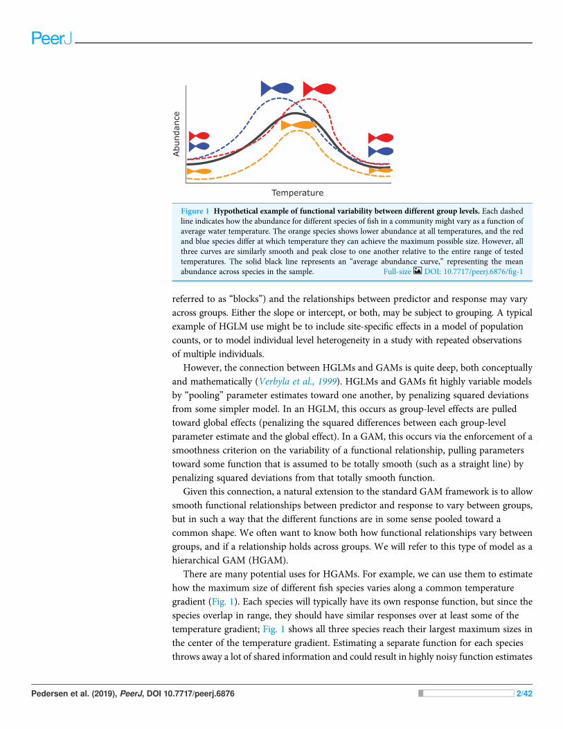
There are many potential uses for HGAMs. For example, we can use them to estimatehow the maximum size of different fish species varies along a common temperaturegradient (Fig. 1). Each species will typically have its own response function, but since thespecies overlap in range, they should have similar responses over at least some of thetemperature gradient; Fig. 1 shows all three species reach their largest maximum sizes inthe center of the temperature gradient. Estimating a separate function for each speciesthrows away a lot of shared information and could result in highly noisy function estimates

Temperature

Abu

ndan

ce

Figure 1 Hypothetical example of functional variability between different group levels. Each dashedline indicates how the abundance for different species of fish in a community might vary as a function ofaverage water temperature. The orange species shows lower abundance at all temperatures, and the redand blue species differ at which temperature they can achieve the maximum possible size. However, allthree curves are similarly smooth and peak close to one another relative to the entire range of testedtemperatures. The solid black line represents an “average abundance curve,” representing the meanabundance across species in the sample. Full-size DOI: 10.7717/peerj.6876/fig-1

Pedersen et al. (2019), PeerJ, DOI 10.7717/peerj.6876 2/42

http://dx.doi.org/10.7717/peerj.6876/fig-1


https://peerj.com/

if there were only a few data points for each species. Estimating a single averagerelationship could result in a function that did not predict any specific group well. In ourexample, using a single global temperature-size relationship (Fig. 1, solid line) wouldmiss that the three species have distinct temperature optima, and that the orange species issignificantly smaller at all temperatures than the other two (Fig. 1). We prefer ahierarchical model that includes a global temperature-size curve plus species-specificcurves that were penalized to be close to the mean function.

This paper discusses several approaches to group-level smoothing, and correspondingtrade-offs. We focus on fitting HGAMs with the popular mgcv package (Wood, 2011)for the R statistical programming language (R Development Core Team, 2018), whichallows for a variety of HGAM model structures and fitting strategies. We discuss optionsavailable to the modeller and practical and theoretical reasons for choosing them.We demonstrate the different approaches across a range of case studies.

This paper is divided into five sections. Part II is a brief review of how GAMs work andtheir relation to hierarchical models. In part III, we discuss different HGAM formulations,what assumptions each model makes about how information is shared between groups,and the different ways of specifying these models in mgcv. In part IV, we work throughexample analyses using this approach, to demonstrate the modeling process and howHGAMs can be incorporated into the ecologist’s quantitative toolbox. Finally, in part V,we discuss some of the computational and statistical issues involved in fitting HGAMsin mgcv. We have also included all the code needed to reproduce the results in thismanuscript in Supplemental Code (online), and on the GitHub repository associated withthis paper: github.com/eric-pedersen/mixed-effect-gams.

A REVIEW OF GENERALIZED ADDITIVE MODELSThe generalized linear model (GLM; McCullagh & Nelder, 1989) relates the mean of aresponse (y) to a linear combination of explanatory variables. The response is assumedto be conditionally distributed according to some exponential family distribution(e.g., binomial, Poisson or Gamma distributions for trial, count or strictly positive realresponses, respectively). The GAM (Hastie & Tibshirani, 1990; Ruppert, Wand & Carroll,2003;Wood, 2017a) allows the relationships between the explanatory variables (henceforthcovariates) and the response to be described by smooth curves (usually splines(De Boor, 1978), but potentially other structures). In general, we have models of the form:

E Yð Þ ¼ g�1 b0 þXJj¼1

fjðxjÞ !

;

where EðYÞ is the expected value of the response Y (with an appropriate distributionand link function g), fj is a smooth function of the covariate xj, β0 is an intercept term,and g-1 is the inverse link function. Hereafter, we will refer to these smooth functionsas smoothers. In the example equation above, there are j smoothers and each is afunction of only one covariate, though it is possible to construct smoothers ofmultiple variables.


http://dx.doi.org/10.7717/peerj.6876#supplemental-information



https://peerj.com/

Each smoother fj is represented by a sum of K simpler, fixed basis functions (bj,k)multiplied by corresponding coefficients (βj,k), which need to be estimated:

fjðxjÞ ¼XKk¼1

bj;kbj;kðxjÞ:

K, referred to as “basis size,” “basis complexity,” or “basis richness,” determines themaximum complexity of each smoother.

It would seem that large basis size could lead to overfitting, but this is counteracted by asmoothing penalty that influences basis function coefficients so as to prevent excesswiggliness and ensure appropriate complexity of each smoother. For each smoother, one(or more) penalty matrices (S), specific to the form of the basis functions, is pre- andpost-multiplied by the parameter vector β to calculate the penalty (βTSβ). A penalty term isthen subtracted from the model log-likelihood L, controlling the trade-off via a smoothingparameter (l). The penalized log-likelihood used to fit the model is thus:

L� �bTSb

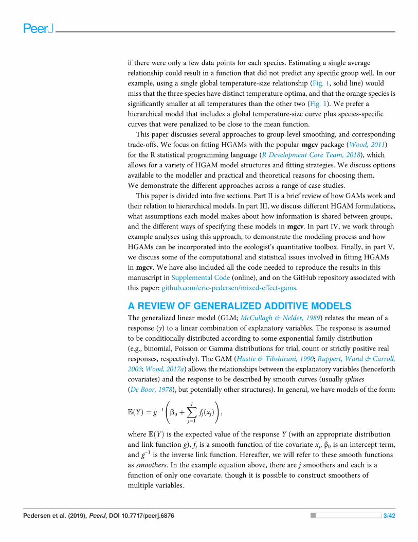
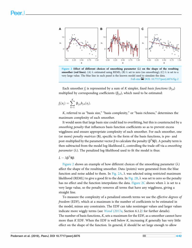
Figure 2 shows an example of how different choices of the smoothing parameter (l)affect the shape of the resulting smoother. Data (points) were generated from the bluefunction and noise added to them. In Fig. 2A, l was selected using restricted maximumlikelihood (REML) to give a good fit to the data. In Fig. 2B, l was set to zero so the penaltyhas no effect and the function interpolates the data. Figure 2C shows when l is set to avery large value, so the penalty removes all terms that have any wiggliness, giving astraight line.

To measure the complexity of a penalized smooth terms we use the effective degrees offreedom (EDF), which at a maximum is the number of coefficients to be estimated inthe model, minus any constraints. The EDF can take noninteger values and larger valuesindicate more wiggly terms (see Wood (2017a, Section 6.1.2) for further details).The number of basis functions, K, sets a maximum for the EDF, as a smoother cannot havemore than K EDF. When the EDF is well below K, increasing K generally has very littleeffect on the shape of the function. In general, K should be set large enough to allow

0

10

0.00 0.25 0.50 0.75 1.00x

y

A

0

10

0.00 0.25 0.50 0.75 1.00x

y

B

0

10

0.00 0.25 0.50 0.75 1.00x

y

C

Figure 2 Effect of different choices of smoothing parameter (λ) on the shape of the resultingsmoother (red lines). (A) l estimated using REML; (B) l set to zero (no smoothing); (C) l is set to avery large value. The blue line in each panel is the known model used to simulate the data.

Full-size DOI: 10.7717/peerj.6876/fig-2




https://peerj.com/

for potential variation in the smoother while still staying low enough to keep computationtime low (see section “Computational and Statistical Issues When Fitting HGAMs” formore on this). In mgcv, the function mgcv::gam.check can be used to determine if Khas been set too low.

Random effects are also “smooths” in this framework. In this case, the penalty matrix isthe inverse of the correlation matrix of the basis function coefficients (Kimeldorf &Wahba,1970; Wood, 2017a). For a simple single-level random effect to account for variationin group means (intercepts) there will be one basis function for each level of the groupingvariable. The basis function takes a value of 1 for any observation in that group and 0for any observation not in the group. The penalty matrix for these terms is a g by g identitymatrix, where g is the number of groups. This means that each group-level coefficient willbe penalized in proportion to its squared deviation from zero. This is equivalent tohow random effects are estimated in standard mixed effect models. The penalty term isproportional to the inverse of the variance of the fixed effect estimated by standardhierarchical model software (Verbyla et al., 1999).

This connection between random effects and splines extends beyond the varying-intercept case. Any single-penalty basis-function representation of a smooth can betransformed so that it can be represented as a combination of a random effect with anassociated variance, and possibly one or more fixed effects. See Verbyla et al. (1999)or Wood, Scheipl & Faraway (2013) for a more detailed discussion on the connectionsbetween these approaches.

Basis types and penalty matricesThe range of smoothers are useful for contrasting needs and have different associatedpenalty matrices for their basis function coefficients. In the examples in this paper, we willuse three types of smoothers: thin plate regression splines (TPRS), cyclic cubic regressionsplines (CRS), and random effects.

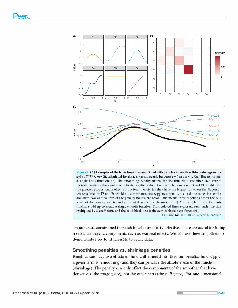
Thin plate regression splines (Wood, 2003) are a general purpose spline basis which canbe used for problems in any number of dimensions, provided one can assume that theamount of smoothing in any of the covariates is the same (so called isotropy or rotationalinvariance). TPRS, like many splines, use a penalty matrix made up of terms based onthe integral of the squared derivatives of basis functions across their range (see Wood(2017a) page 216 for details on this penalty). Models that overfit the data will tend to havelarge derivatives, so this penalization reduces wiggliness. We will refer to the order ofpenalized derivatives by m. Typically, TPRS are second-order (m = 2), meaning that thepenalty is proportionate to the integral of the squared second derivative. However,TPRS may be of lower order (m = 1, penalizing squared first derivatives), or higher order(m > 2, penalizing squared higher order derivatives). We will see in section “What areHierarchical GAMs?” how lower-order TPRS smoothers are useful in fitting HGAMs.Example basis functions and penalty matrix S for a m = 2 TPRS with six basis functionsfor evenly spaced data are shown in Fig. 3.

Cyclic cubic regression splines are another smoother that penalizes the squared secondderivative of the smooth across the function. In cyclic CRS the start and end of the



https://peerj.com/

smoother are constrained to match in value and first derivative. These are useful for fittingmodels with cyclic components such as seasonal effects. We will use these smoothers todemonstrate how to fit HGAMs to cyclic data.

Smoothing penalties vs. shrinkage penaltiesPenalties can have two effects on how well a model fits: they can penalize how wigglya given term is (smoothing) and they can penalize the absolute size of the function(shrinkage). The penalty can only affect the components of the smoother that havederivatives (the range space), not the other parts (the null space). For one-dimensional

F4 F5 F6

F1 F2 F3

0 0.5 1 0 0.5 1 0 0.5 1

−2

−1

0

1

−2

−1

0

1

x

valu

e

F6

F5

F4

F3

F2

F1

F1 F2 F3 F4 F5 F6

0

0.5

1penalty

BA

F1 × 0.39

F2 × − 0.4F3 × 0.26

F4 × 0.33

F5 × − 0.1

F6 × 0.12

−1.5

−1.0

−0.5

0.0

0.5

0.0 0.3 0.6 0.9x

valu

e

C

Figure 3 (A) Examples of the basis functions associated with a six basis function thin plate regressionspline (TPRS,m = 2), calculated for data, x, spread evenly between x = 0 and x = 1. Each line representsa single basis function. (B) The smoothing penalty matrix for the thin plate smoother. Red entriesindicate positive values and blue indicate negative values. For example, functions F3 and F4 would havethe greatest proportionate effect on the total penalty (as they have the largest values on the diagonal),whereas function F5 and F6 would not contribute to the wiggliness penalty at all (all the values in the fifthand sixth row and column of the penalty matrix are zero). This means these functions are in the nullspace of the penalty matrix, and are treated as completely smooth. (C) An example of how the basisfunctions add up to create a single smooth function. Thin colored lines represent each basis functionmultiplied by a coefficient, and the solid black line is the sum of those basis functions.





https://peerj.com/

TPRS (when m = 2), this means that there is a linear term (F5) left in the model, evenwhen the penalty is in full force (as l / ∞), as shown in Fig. 3. (This is also whyFig. 2C shows a linear, rather than flat, fit to the data). The random effects smoother wediscussed earlier is an example of a pure shrinkage penalty; it penalizes all deviations awayfrom zero, no matter the pattern of those deviations. This will be useful later in “What areHierarchical GAMs?,” where we use random effect smoothers as one of the componentsof a HGAM.

Interactions between smooth termsIt is also possible to create interactions between covariates with different smoothers(or degrees of smoothness) assumed for each covariate, using tensor products. For instance,if one wanted to estimate the interacting effects of temperature and time (in seconds)on some outcome, it would not make sense to use a two-dimensional TPRS smoother, asthat would assume that a one degree change in temperature would equate to a 1 s changein time. Instead, a tensor product allows us to create a new set of basis functions thatallow for each marginal function (here temperature and time) to have its own marginalsmoothness penalty. A different basis can be used in each marginal smooth, as required forthe data at hand.

There are two approaches used in mgcv for generating tensor products. The firstapproach (Wood, 2006a) essentially creates an interaction of each pair of basis functionsfor each marginal term, and a penalty for each marginal term that penalizes theaverage wiggliness in that term; in mgcv, these are created using the te() function.The second approach (Wood, Scheipl & Faraway, 2013) separates each penalty intopenalized (range space) and unpenalized components (null space; components that don’thave derivatives, such as intercept and linear terms in a one-dimensional cubic spline).This approach creates new basis functions and penalties for all pair-wise combinations ofpenalized and unpenalized components between all pairs of marginal bases; in mgcv,these are created using the t2() function. The advantage of the first method is that itrequires fewer smoothing parameters, so is faster to estimate in most cases. The advantageof the second method is that the tensor products created this way only have a single penaltyassociated with each marginal basis (unlike the te() approach, where each penaltyapplies to all basis functions), so it can be fitted using standard mixed effect software suchas lme4 (Bates et al., 2015).

Comparison to hierarchical linear modelsHierarchical generalized linear models (Gelman, 2006; HGLMs; also referred to asgeneralized linear mixed effect models, multilevel models, etc.; e.g., Bolker et al., 2009) arean extension of regression modeling that allows the inclusion of terms in the modelthat account for structure in the data—the structure is usually of the form of a nesting ofthe observations. For example, in an empirical study, individuals may be nested withinsample sites, sites are nested within forests, and forests within provinces. The depth of thenesting is limited by the fitting procedure and number of parameters to estimate.



https://peerj.com/

Hierarchical generalized linear models are a highly flexible way to think about groupingin ecological data; the groupings used in models often refer to the spatial or temporal scaleof the data (McMahon & Diez, 2007) though can be based on any useful grouping.

We would like to be able to think about the groupings in our data in a similar way, evenwhen the covariates in our model are related to the response in a smooth way. The nextsection investigates the extension of the smoothers we showed above to the case whereobservations are grouped and we model group-level smoothers.

WHAT ARE HIERARCHICAL GAMS?What do we mean by hierarchical smoothers?In this section, we will describe how to model intergroup variability using smooth curvesand how to fit these models usingmgcv. All models were fitted usingmgcv version 1.8–26(Wood, 2011). Model structure is key in this framework, so we start with three modelchoices:

1. Should each group have its own smoother, or will a common smoother suffice?

2. Do all of the group-specific smoothers have the same wiggliness, or should each grouphave its own smoothing parameter?

3. Will the smoothers for each group have a similar shape to one another—a shared globalsmoother?

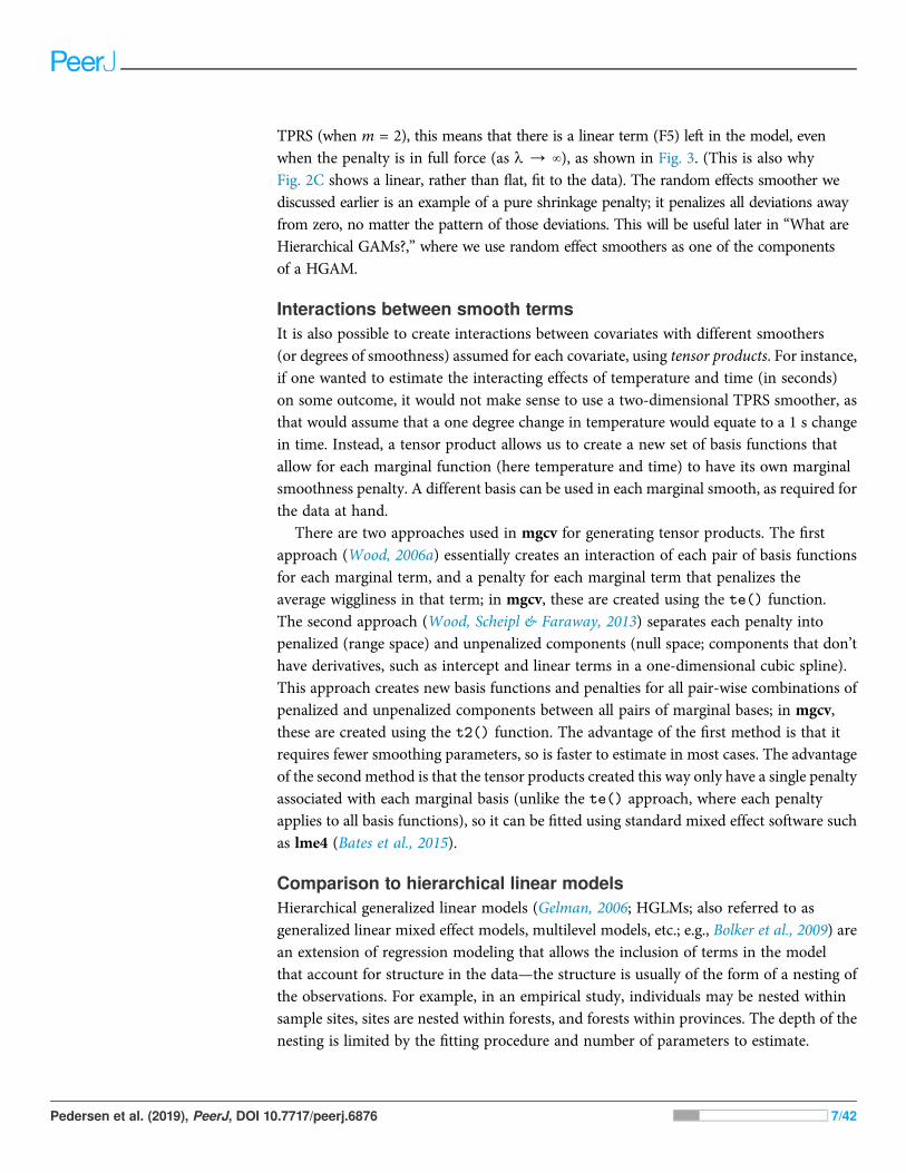
These three choices result in five possible models (Fig. 4):

1. A single common smoother for all observations; We will refer to this as model G, as itonly has a Global smoother.

2. A global smoother plus group-level smoothers that have the same wiggliness. We willrefer to this as model GS (for Global smoother with individual effects that have a Sharedpenalty).

3. A global smoother plus group-level smoothers with differing wiggliness. We will refer tothis as model GI (for Global smoother with individual effects that have Individualpenalties).

4. Group-specific smoothers without a global smoother, but with all smoothers having thesame wiggliness. We will refer to this as model S.

5. Group-specific smoothers with different wiggliness. We will refer to this as model I.

It is important to note that “similar wiggliness” and “similar shape” are two distinctconcepts; functions can have very similar wiggliness but very different shapes. Wigglinessmeasures how quickly a function changes across its range, and it is easy to constructtwo functions that differ in shape but have the same wiggliness. For this paper, we considertwo functions to have similar shape if the average squared distance between the functionsis small (assuming the functions have been scaled to have a mean value of zero acrosstheir ranges). This definition is somewhat restricted; for instance, a cyclic function wouldnot be considered to have the same shape as a phase-shifted version of the same function,



https://peerj.com/

nor would two normal distributions with the same mean but different standarddeviations. The benefit of this definition of shape, however, is that it is straightforward totranslate into penalties akin to those described in the section “A Review of GeneralizedAdditive Models.” Figure 4, model S illustrates the case where models have differentshapes. Similarly, two curves could have very similar overall shape, but differ in theirwiggliness. For instance, one function could be equal to another plus a high-frequencyoscillation term. Figure 4, model GI illustrates this.

We will discuss the trade-offs between different models and guidelines about when eachof these models is appropriate in the section “Computational and statistical issues whenfitting HGAMs”. The remainder of this section will focus on how to specify each of these fivemodels using mgcv.

model G

model GS

model GI

model S

model I

Shared (Global) trend No shared trend

No group−level trends

Group−level trends

similar sm

oothness(S

hared penalty)

Group−level trends

different smoothness

(Individual penalties)

0 0.5 1 0 0.5 1

−1

0

1

2

−1

0

1

2

−1

0

1

2

x

f(x)

Figure 4 Alternate types of functional variation f(x) that can be fitted with HGAMs. The dashed lineindicates the average function value for all groups, and each solid line indicates the functional value at agiven predictor value for an individual group level. The null model (of no functional relationship betweenthe covariate and outcome, top right), is not explicitly assigned a model name.





https://peerj.com/

Coding hierarchical GAMs in REach of the models in Fig. 4 can be coded straightforwardly in mgcv. We will use twoexample datasets to demonstrate how to code these models (see the Supplemental Code toreproduce these examples):

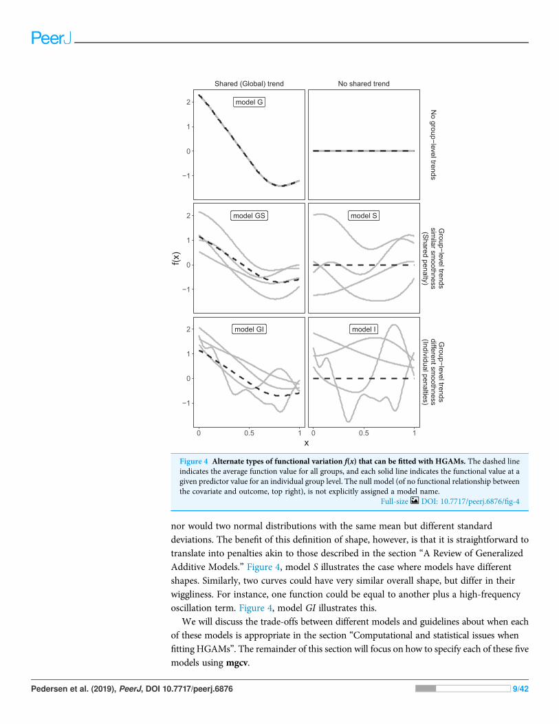
A. The CO2 dataset, available in R via the datasets package. This data is from anexperimental study by Potvin, Lechowicz & Tardif (1990) of CO2 uptake in grassesunder varying concentrations of CO2, measuring how concentration-uptake functionsvaried between plants from two locations (Mississippi and Quebec) and twotemperature treatments (chilled and warm). A total of 12 plants were used and CO2

uptake measured at seven CO2 concentrations for each plant (Fig. 5A). Here, wewill focus on how to use HGAMs to estimate interplant variation in functionalresponses. This data set has been modified from the default version available with R, torecode the Plant variable as an unordered factor Plant_uo1.

B. Data generated from a hypothetical study of bird movement along a migration corridor,sampled throughout the year (see Supplemental Code). This dataset consists ofsimulated sample records of numbers of observed locations of 100 tagged individualseach from six species of bird, at 10 locations along a latitudinal gradient, with oneobservation taken every 4 weeks. Counts were simulated randomly for each species ineach location and week by creating a species-specific migration curve that gave theprobability of finding an individual of a given species in a given location, then simulatedthe distribution of individuals across sites using a multinomial distribution, andsubsampling that using a binomial distribution to simulate observation error (i.e., notevery bird present at a location would be detected). The data set (bird_move)consists of the variables count, latitude, week, and species (Fig. 5B). This exampleallows us to demonstrate how to fit these models with interactions and with non-normal(count) data. The true model used to generate this data was model GS: a single globalfunction plus species-specific deviations around that global function.

Throughout the examples we use REML to estimate model coefficients and smoothingparameters. We strongly recommend using either REML or marginal likelihood (ML)rather than the default generalized cross-validation criteria when fitting GAMs, for thereasons outlined inWood (2011). In each case some data processing and manipulation hasbeen done to obtain the graphics and results below. See Supplemental Code for detailson data processing steps. To illustrate plots, we will be using the draw() function from thegratia package. This package was developed by one of the authors (Simpson, 2018) as aset of tools to extend plotting and analysis of mgcv models. While mgcv has plottingcapabilities (through plot() methods), gratia expands these by creating ggplot2 objects(Wickham, 2016) that can be more easily extended and modified.

A single common (global) smoother for all observations (Model G)We start with the simplest model from the framework and include many details here toensure that readers are comfortable with the terminology and R functions.

1 Note thatmgcv requires that grouping orcategorical variables be coded as factorsin R; it will raise an error message ifpassed data coded as characters. It is alsoimportant to know whether the factor iscoded as ordered or unordered (see?factor for more details on this). Thismatters when fitting group-levelsmoothers using the by= argument (as isused for fitting models GI and I, shownbelow). If the factor is unordered, mgcvwill set up a model with one smoother foreach grouping level. If the factor isordered, mgcv will set any basis func-tions for the first grouping level to zero.In model GI the ungrouped smootherwill then correspond to the first groupinglevel, rather than the average functionalresponse, and the group-specificsmoothers will correspond to deviationsfrom the first group. In model I, using anordered factor will result in the firstgroup not having a smoother associatedwith it at all.






https://peerj.com/

For our CO2 data set, we will model loge(uptake) as a function of two smoothers: aTPRS of loge-concentration, and a random effect for Plant_uo to model plant-specificintercepts. Mathematically:

logeðuptakeiÞ ¼ f ðlogeðconciÞÞ þ fPlant uo þ ei

where fPlant uo is the random effect for plant and εi is a Gaussian error term. Here, weassume that loge(uptakei) is normally distributed.In R we can write our model as:

CO2_modG <- gam(log(uptake) ∼ s(log(conc), k=5, bs="tp") +

s(Plant_uo, k=12, bs="re"),

data=CO2, method="REML", family="gaussian")

This is a common GAM structure, with a single smooth term for each variable.Specifying the model is similar to specifying a GLM in R via glm(), with the addition ofs() terms to include one-dimensional or isotropic multidimensional smoothers. The firstargument to s() are the terms to be smoothed, the type of smoother to be used forthe term is specified by the bs argument, and the maximum number of basis functionsis specified by k. There are different defaults in mgcv for K, depending on the type ofsmoother chosen; here we use a TPRS smoother (bs="tp") for the concentrationsmoother, and set k=5 as there are only seven separate values of concentrationmeasured, so the default k=10 (for TPRS) would be too high; further, setting k=5 saves oncomputational time (see section “Computational and Statistical Issues When FittingHGAMs”). The random effect smoother (bs="re") that we used for the Plant_uo factoralways has a k value equal to the number of levels in the grouping variable (here, 12).We specified k=12 just to make this connection apparent.

10

20

30

40

250 500 750 1000

CO2 concentration (mL L−1)

CO

2 up

take

( μm

ol m

−2)

A

sp4 sp5 sp6

sp1 sp2 sp3

0 10 20 30 40 50 0 10 20 30 40 50 0 10 20 30 40 50

20

40

60

20

40

60

Week

Latit

ude

Count 5 10 15 20

B

Figure 5 Example data sets used throughout section “What are Hierarchical GAMs?” (A) Grass CO2

uptake vs. CO2 concentration for 12 individual plants. Color and line type included to distinguishindividual plant trends. (B) Simulated data set of bird migration, with point size corresponding to weeklycounts of six species along a latitudinal gradient (zeros excluded for clarity).





https://peerj.com/

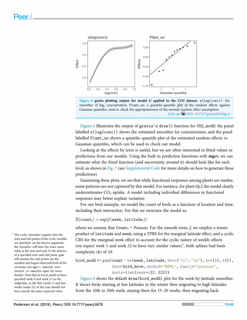
Figure 6 Illustrates the output of gratia's draw() function for CO2_modG: the panellabelled s(log(conc)) shows the estimated smoother for concentration, and the panellabelled Plant_uo shows a quantile–quantile plot of the estimated random effects vs.Gaussian quantiles, which can be used to check our model.

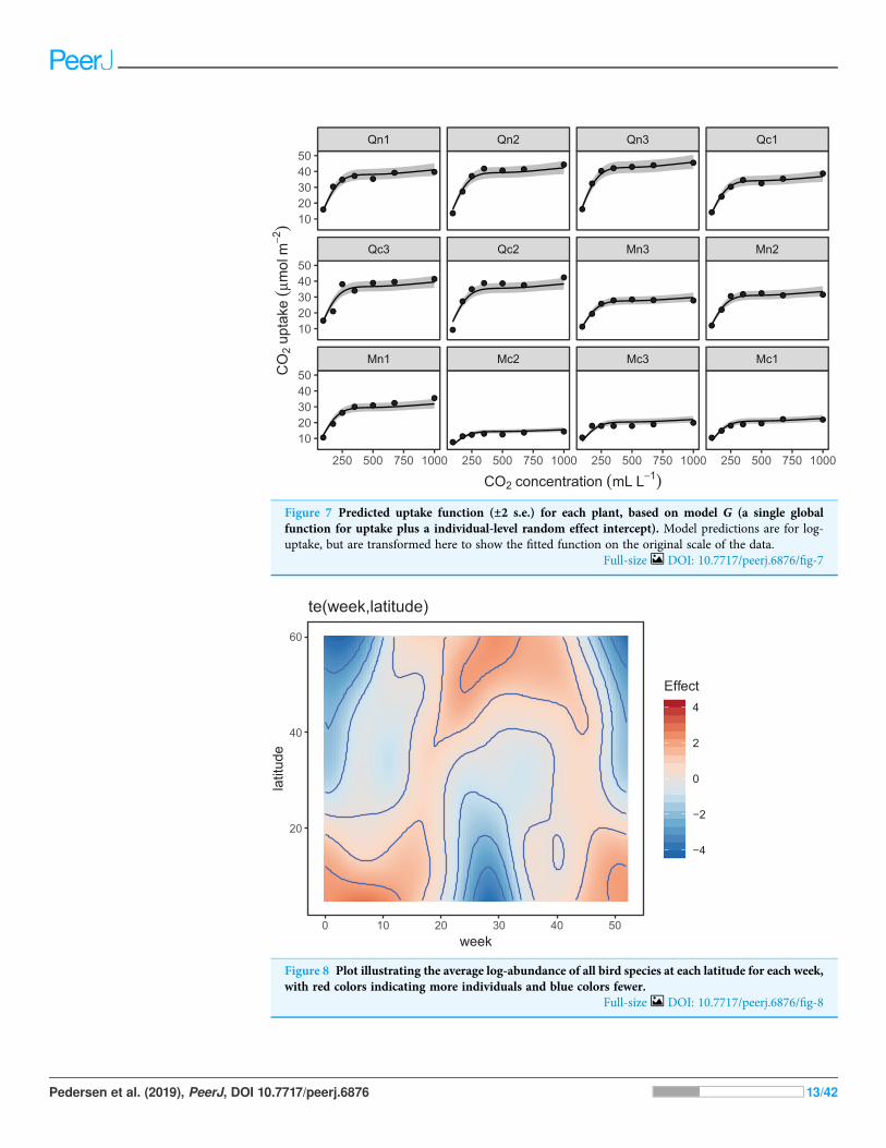
Looking at the effects by term is useful, but we are often interested in fitted values orpredictions from our models. Using the built in prediction functions with mgcv, we canestimate what the fitted function (and uncertainty around it) should look like for eachlevel, as shown in Fig. 7 (see Supplemental Code for more details on how to generate thesepredictions).

Examining these plots, we see that while functional responses among plants are similar,some patterns are not captured by this model. For instance, for plant Qc2 the model clearlyunderestimates CO2 uptake. A model including individual differences in functionalresponses may better explain variation.

For our bird example, we model the count of birds as a function of location and time,including their interaction. For this we structure the model as:

EðcountiÞ ¼ expðf ðweeki; latitudeiÞÞwhere we assume that Counti ∼ Poisson. For the smooth term, f, we employ a tensorproduct of latitude and week, using a TPRS for the marginal latitude effect, and a cyclicCRS for the marginal week effect to account for the cyclic nature of weekly effects(we expect week 1 and week 52 to have very similar values)2, both splines had basiscomplexity (k) of 10.

bird_modG <- gam(count ∼ te(week, latitude, bs=c("cc", "tp"), k=c(10, 10)),

data=bird_move, method="REML", family="poisson",

knots=list(week=c(0, 52)))

Figure 8 shows the default draw(bird_modG) plot for the week-by-latitude smoother.It shows birds starting at low latitudes in the winter then migrating to high latitudesfrom the 10th to 20th week, staying there for 15–20 weeks, then migrating back.

−0.6

−0.3

0.0

0.3

4.5 5.0 5.5 6.0 6.5 7.0log(conc)

Effe

ct

s(log(conc))

●●

●●

●

●●

●●

●●

●

●

−0.75

−0.50

−0.25

0.00

0.25

−1 0 1Gaussian quantiles

Effe

cts

Plant_uo

Figure 6 gratia plotting output for model G applied to the CO2 dataset. s(log(conc)): thesmoother of loge concentration. Plant_uo: a quantile–quantile plot of the random effects againstGaussian quantiles, used to check the appropriateness of the normal random effect assumption.


2 The cyclic smoother requires that thestart and end points of the cyclic variableare specified, via the knots argument;the smoother will have the exact samevalue at the start and end. In the absenceof a specified start and end point, gamwill assume the end points are thesmallest and largest observed levels of thecovariate (see mgcv::smooth.con-struct.cc.smooth.spec for moredetails). Note that in bird_modGwe havespecified week 0 and week 52 as theendpoints, as the first (week 1) and lastweeks (week 52) of the year should nothave exactly the same expected value.





https://peerj.com/

Mn1 Mc2 Mc3 Mc1

Qc3 Qc2 Mn3 Mn2

Qn1 Qn2 Qn3 Qc1

250 500 750 1000 250 500 750 1000 250 500 750 1000 250 500 750 1000

1020304050

1020304050

1020304050


CO

2 up

take

(μm

ol m

−2)

Figure 7 Predicted uptake function (±2 s.e.) for each plant, based on model G (a single globalfunction for uptake plus a individual-level random effect intercept). Model predictions are for log-uptake, but are transformed here to show the fitted function on the original scale of the data.


20

40

60

0 10 20 30 40 50week

latit

ude

−4

−2

0

2

4

Effect

te(week,latitude)

Figure 8 Plot illustrating the average log-abundance of all bird species at each latitude for each week,with red colors indicating more individuals and blue colors fewer.






https://peerj.com/

However, the plot also indicates a large amount of variability in the timing of migration.The source of this variability is apparent when we look at the timing of migration of eachspecies (cf. Fig. 5B).

All six species in Fig. 5B show relatively precise migration patterns, but they differ in thetiming of when they leave their winter grounds and the amount of time they spend attheir summer grounds. Averaging over all of this variation results in a relatively imprecise(diffuse) estimate of migration timing (Fig. 8), and viewing species-specific plots ofobserved vs. predicted values (Fig. 9), it is apparent that the model fits some of the speciesbetter than others. This model could potentially be improved by adding intergroupvariation in migration timing. The rest of this section will focus on how to model this typeof variation.

A single common smoother plus group-level smoothers that have thesame wiggliness (model GS)Model GS is a close analogue to a GLMM with varying slopes: all groups have similarfunctional responses, but intergroup variation in responses is allowed. This approachworks by allowing each grouping level to have its own functional response, but penalizingfunctions that are too far from the average.

This can be coded inmgcv by explicitly specifying one term for the global smoother (as inmodel G above) then adding a second smooth term specifying the group-level smooth terms,

sp4 sp5 sp6

sp1 sp2 sp3

0 5 10 0 5 10 0 5 10

0

5

10

15

20

0

5

10

15

20

Predicted count

Obs

erve

d co

unt

Figure 9 Observed counts by species vs. predicted counts from bird_modG (1–1 line added asreference). If our model fitted well we would expect that all species should show similar patterns ofdispersion around the 1-1 line (and as we are assuming the data is Poisson, the variance around the meanshould equal the mean). Instead we see that variance around the predicted value is much higher forspecies 1 and 6. Full-size DOI: 10.7717/peerj.6876/fig-9




https://peerj.com/

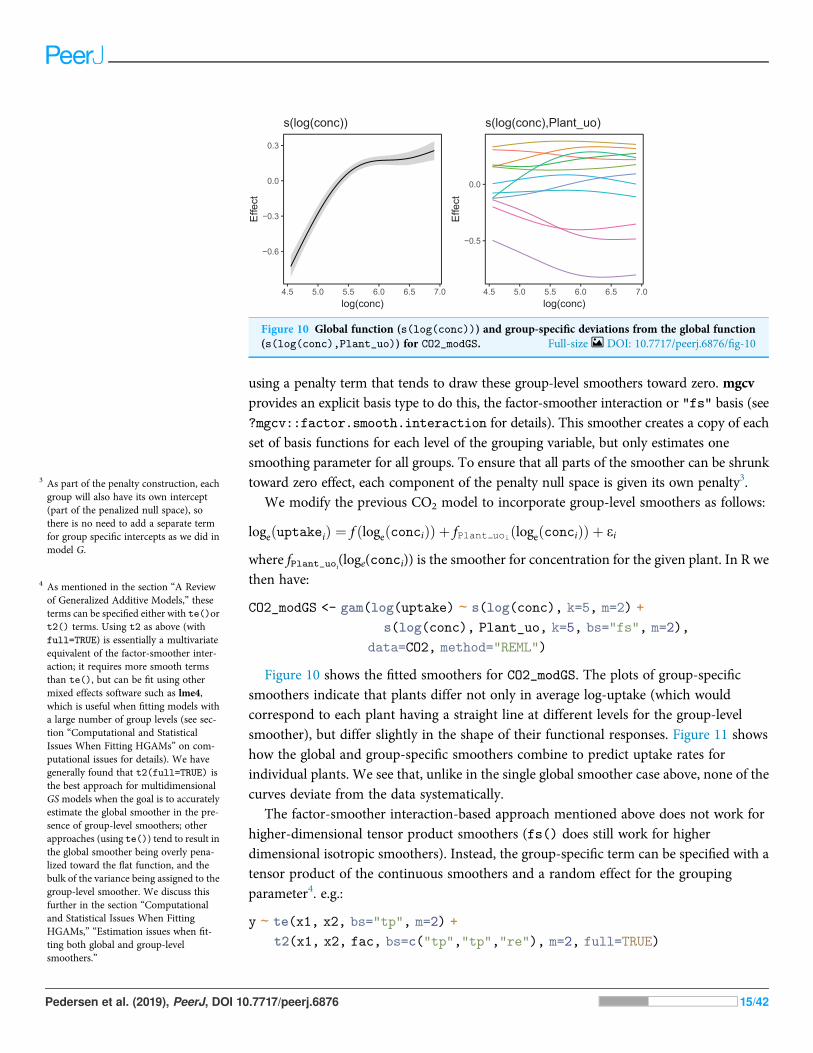
using a penalty term that tends to draw these group-level smoothers toward zero. mgcvprovides an explicit basis type to do this, the factor-smoother interaction or "fs" basis (see?mgcv::factor.smooth.interaction for details). This smoother creates a copy of eachset of basis functions for each level of the grouping variable, but only estimates onesmoothing parameter for all groups. To ensure that all parts of the smoother can be shrunktoward zero effect, each component of the penalty null space is given its own penalty3.

We modify the previous CO2 model to incorporate group-level smoothers as follows:

logeðuptakeiÞ ¼ f ðlogeðconciÞÞ þ fPlant uoiðlogeðconciÞÞ þ ei

where fPlant_uoi(loge(conci)) is the smoother for concentration for the given plant. In R wethen have:

CO2_modGS <- gam(log(uptake) ∼ s(log(conc), k=5, m=2) +

s(log(conc), Plant_uo, k=5, bs="fs", m=2),

data=CO2, method="REML")

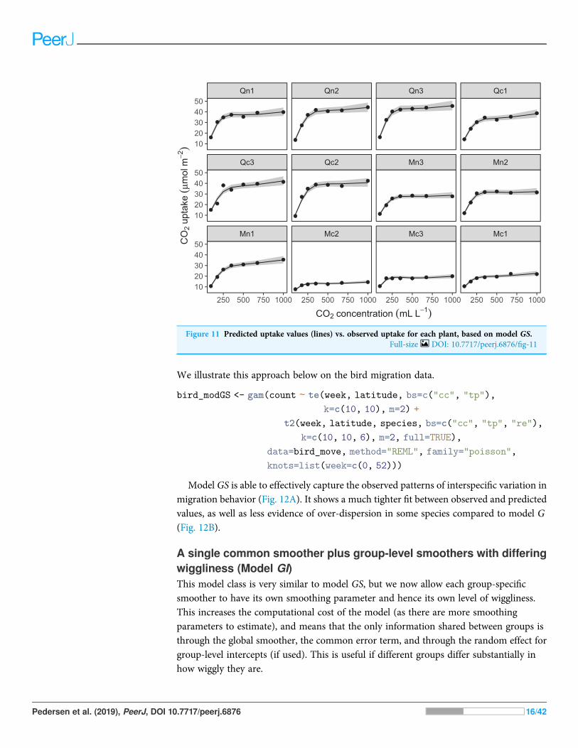
Figure 10 shows the fitted smoothers for CO2_modGS. The plots of group-specificsmoothers indicate that plants differ not only in average log-uptake (which wouldcorrespond to each plant having a straight line at different levels for the group-levelsmoother), but differ slightly in the shape of their functional responses. Figure 11 showshow the global and group-specific smoothers combine to predict uptake rates forindividual plants. We see that, unlike in the single global smoother case above, none of thecurves deviate from the data systematically.

The factor-smoother interaction-based approach mentioned above does not work forhigher-dimensional tensor product smoothers (fs() does still work for higherdimensional isotropic smoothers). Instead, the group-specific term can be specified with atensor product of the continuous smoothers and a random effect for the groupingparameter4. e.g.:

y ∼ te(x1, x2, bs="tp", m=2) +

t2(x1, x2, fac, bs=c("tp","tp","re"), m=2, full=TRUE)

−0.6

−0.3

0.0

0.3

4.5 5.0 5.5 6.0 6.5 7.0log(conc)

Effe

ct

s(log(conc))

−0.5

0.0

4.5 5.0 5.5 6.0 6.5 7.0log(conc)

Effe

ct

s(log(conc),Plant_uo)

Figure 10 Global function (s(log(conc))) and group-specific deviations from the global function(s(log(conc),Plant_uo)) for CO2_modGS. Full-size DOI: 10.7717/peerj.6876/fig-10

3 As part of the penalty construction, eachgroup will also have its own intercept(part of the penalized null space), sothere is no need to add a separate termfor group specific intercepts as we did inmodel G.

4 As mentioned in the section “A Reviewof Generalized Additive Models,” theseterms can be specified either with te()ort2() terms. Using t2 as above (withfull=TRUE) is essentially a multivariateequivalent of the factor-smoother inter-action; it requires more smooth termsthan te(), but can be fit using othermixed effects software such as lme4,which is useful when fitting models witha large number of group levels (see sec-tion “Computational and StatisticalIssues When Fitting HGAMs” on com-putational issues for details). We havegenerally found that t2(full=TRUE) isthe best approach for multidimensionalGS models when the goal is to accuratelyestimate the global smoother in the pre-sence of group-level smoothers; otherapproaches (using te()) tend to result inthe global smoother being overly pena-lized toward the flat function, and thebulk of the variance being assigned to thegroup-level smoother. We discuss thisfurther in the section “Computationaland Statistical Issues When FittingHGAMs,” “Estimation issues when fit-ting both global and group-levelsmoothers.”




https://peerj.com/

We illustrate this approach below on the bird migration data.

bird_modGS <- gam(count ∼ te(week, latitude, bs=c("cc", "tp"),

k=c(10, 10), m=2) +

t2(week, latitude, species, bs=c("cc", "tp", "re"),

k=c(10, 10, 6), m=2, full=TRUE),



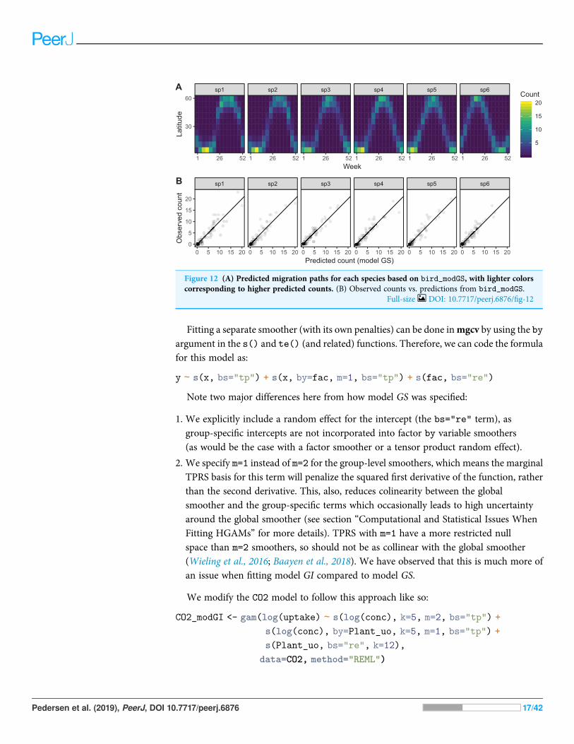
Model GS is able to effectively capture the observed patterns of interspecific variation inmigration behavior (Fig. 12A). It shows a much tighter fit between observed and predictedvalues, as well as less evidence of over-dispersion in some species compared to model G(Fig. 12B).

A single common smoother plus group-level smoothers with differingwiggliness (Model GI)This model class is very similar to model GS, but we now allow each group-specificsmoother to have its own smoothing parameter and hence its own level of wiggliness.This increases the computational cost of the model (as there are more smoothingparameters to estimate), and means that the only information shared between groups isthrough the global smoother, the common error term, and through the random effect forgroup-level intercepts (if used). This is useful if different groups differ substantially inhow wiggly they are.

Mn1 Mc2 Mc3 Mc1

Qc3 Qc2 Mn3 Mn2

Qn1 Qn2 Qn3 Qc1

250 500 750 1000 250 500 750 1000 250 500 750 1000 250 500 750 1000

1020304050

1020304050

1020304050


CO

2up

take

(μm

olm

−2)

Figure 11 Predicted uptake values (lines) vs. observed uptake for each plant, based on model GS.Full-size DOI: 10.7717/peerj.6876/fig-11




https://peerj.com/

Fitting a separate smoother (with its own penalties) can be done inmgcv by using the byargument in the s() and te() (and related) functions. Therefore, we can code the formulafor this model as:

y ∼ s(x, bs="tp") + s(x, by=fac, m=1, bs="tp") + s(fac, bs="re")

Note two major differences here from how model GS was specified:

1. We explicitly include a random effect for the intercept (the bs="re" term), asgroup-specific intercepts are not incorporated into factor by variable smoothers(as would be the case with a factor smoother or a tensor product random effect).

2. We specify m=1 instead of m=2 for the group-level smoothers, which means the marginalTPRS basis for this term will penalize the squared first derivative of the function, ratherthan the second derivative. This, also, reduces colinearity between the globalsmoother and the group-specific terms which occasionally leads to high uncertaintyaround the global smoother (see section “Computational and Statistical Issues WhenFitting HGAMs” for more details). TPRS with m=1 have a more restricted nullspace than m=2 smoothers, so should not be as collinear with the global smoother(Wieling et al., 2016; Baayen et al., 2018). We have observed that this is much more ofan issue when fitting model GI compared to model GS.

We modify the CO2 model to follow this approach like so:

CO2_modGI <- gam(log(uptake) ∼ s(log(conc), k=5, m=2, bs="tp") +

s(log(conc), by=Plant_uo, k=5, m=1, bs="tp") +

s(Plant_uo, bs="re", k=12),


sp1 sp2 sp3 sp4 sp5 sp6

1 26 52 1 26 52 1 26 52 1 26 52 1 26 52 1 26 52

30

60

Week

Latit

ude

5

10

15

20Count

A

sp1 sp2 sp3 sp4 sp5 sp6

0 5 10 15 20 0 5 10 15 20 0 5 10 15 20 0 5 10 15 20 0 5 10 15 20 0 5 10 15 200

5

10

15

20

Predicted count (model GS)

Obs

erve

d co

unt

B

Figure 12 (A) Predicted migration paths for each species based on bird_modGS, with lighter colorscorresponding to higher predicted counts. (B) Observed counts vs. predictions from bird_modGS.





https://peerj.com/

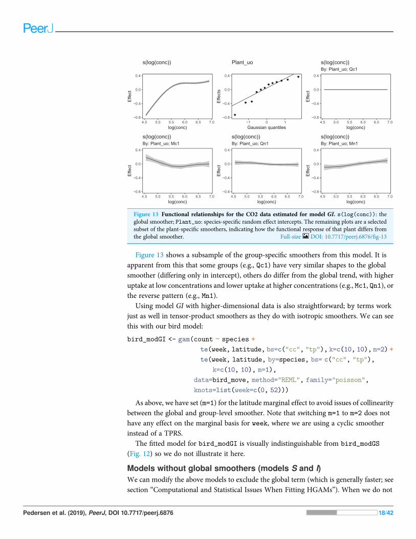
Figure 13 shows a subsample of the group-specific smoothers from this model. It isapparent from this that some groups (e.g., Qc1) have very similar shapes to the globalsmoother (differing only in intercept), others do differ from the global trend, with higheruptake at low concentrations and lower uptake at higher concentrations (e.g., Mc1, Qn1), orthe reverse pattern (e.g., Mn1).

Using model GI with higher-dimensional data is also straightforward; by terms workjust as well in tensor-product smoothers as they do with isotropic smoothers. We can seethis with our bird model:

bird_modGI <- gam(count ∼ species +

te(week, latitude, bs=c("cc", "tp"), k=c(10, 10), m=2) +

te(week, latitude, by=species, bs= c("cc", "tp"),

k=c(10, 10), m=1),



As above, we have set (m=1) for the latitude marginal effect to avoid issues of collinearitybetween the global and group-level smoother. Note that switching m=1 to m=2 does nothave any effect on the marginal basis for week, where we are using a cyclic smootherinstead of a TPRS.

The fitted model for bird_modGI is visually indistinguishable from bird_modGS

(Fig. 12) so we do not illustrate it here.

Models without global smoothers (models S and I)We can modify the above models to exclude the global term (which is generally faster; seesection “Computational and Statistical Issues When Fitting HGAMs”). When we do not

−0.8

−0.4

0.0

0.4

4.5 5.0 5.5 6.0 6.5 7.0log(conc)

Effe

ct

s(log(conc))

−0.8

−0.4

0.0

0.4

−1 0 1Gaussian quantiles

Effe

cts

Plant_uo

−0.8

−0.4

0.0

0.4

4.5 5.0 5.5 6.0 6.5 7.0log(conc)

Effe

ct

By: Plant_uo; Qc1s(log(conc))

−0.8

−0.4

0.0

0.4

4.5 5.0 5.5 6.0 6.5 7.0log(conc)

Effe

ct

By: Plant_uo; Mc1s(log(conc))

−0.8

−0.4

0.0

0.4

4.5 5.0 5.5 6.0 6.5 7.0log(conc)

Effe

ct

By: Plant_uo; Qn1s(log(conc))

−0.8

−0.4

0.0

0.4

4.5 5.0 5.5 6.0 6.5 7.0log(conc)

Effe

ct

By: Plant_uo; Mn1s(log(conc))

Figure 13 Functional relationships for the CO2 data estimated for model GI. s(log(conc)): theglobal smoother; Plant_uo: species-specific random effect intercepts. The remaining plots are a selectedsubset of the plant-specific smoothers, indicating how the functional response of that plant differs fromthe global smoother. Full-size DOI: 10.7717/peerj.6876/fig-13




https://peerj.com/

model the global term, we are allowing each group to be differently shaped withoutrestriction. Though there may be some similarities in the shape of the functions, thesemodels’ underlying assumption is that group-level smooth terms do not share or deviatefrom a common form.

Model SModel S (shared smoothers) is model GS without the global smoother term; this type ofmodel takes the form: y∼s(x, fac, bs="fs") or y∼t2(x1, x2, fac, bs=c("tp",

"tp", "re") in mgcv. This model assumes all groups have the same smoothness, but thatthe individual shapes of the smooth terms are not related. Here, we do not plot thesemodels; the model plots are very similar to the plots for model GS. This will not always bethe case. If in a study there are very few data points in each grouping level (relative tothe strength of the functional relationship of interest), estimates frommodel S will typicallybe much more variable than from model GS; there is no way for the model to shareinformation on function shape between grouping levels without the global smoother. Seesection “Computational and Statistical Issues When Fitting HGAMs” on computationalissues for more on how to choose between different models.

CO2_modS <- gam(log(uptake) ∼ s(log(conc), Plant_uo, k=5, bs="fs", m=2),


bird_modS <- gam(count ∼ t2(week, latitude, species, bs=c("cc", "tp", "re"),

k=c(10, 10, 6), m=2, full=TRUE),



Model I

Model I is model GI without the first term: y∼fac+s(x, by=fac) or y∼fac+te(x1,x2,by=fac) (as above, plots are very similar to model GI).

CO2_modI <- gam(log(uptake) ∼ s(log(conc), by=Plant_uo, k=5, bs="tp", m=2) +

s(Plant_uo, bs="re", k=12),


bird_modI <- gam(count ∼ species + te(week, latitude, by=species,

bs=c("cc", "tp"), k=c(10, 10), m=2),



Comparing different HGAM specificationsThese models can be compared using standard model comparison tools. Model GS andmodel GI will generally be nested in model G (depending on how each model is specified)so comparisons using generalized likelihood ratio tests (GLRTs) may be used to testif group-level smoothers are necessary (if fit using method="ML"). However, we do notcurrently recommend this method. There is not sufficient theory on how accurate



https://peerj.com/

parametric p-values are for comparing these models; there is uncertainty about whatdegrees of freedom to assign to models with varying smoothness, and slightly differentmodel specifications may not result in nested models (See Wood (2017a) Section 6.12.4and ?mgcv::anova.gam for more discussion on using GLRTs to compare GAMs).

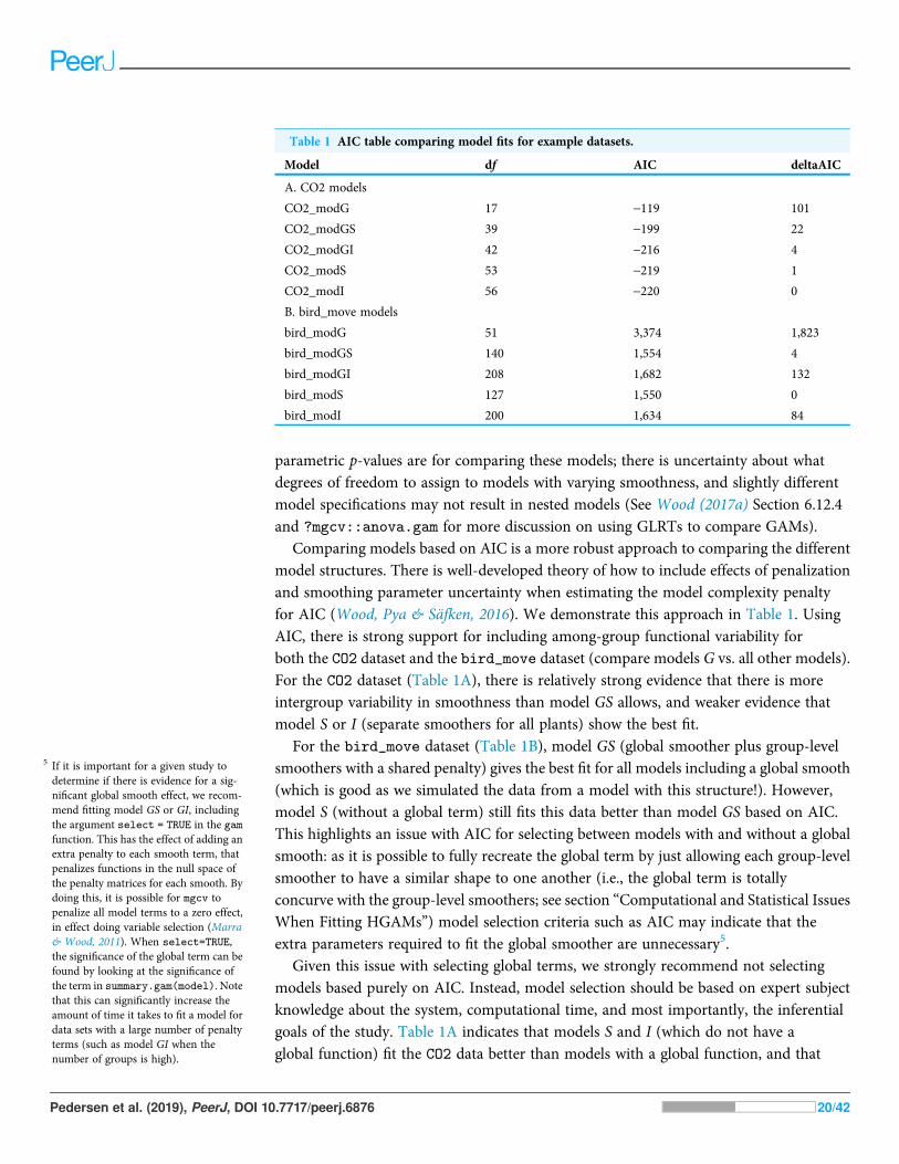
Comparing models based on AIC is a more robust approach to comparing the differentmodel structures. There is well-developed theory of how to include effects of penalizationand smoothing parameter uncertainty when estimating the model complexity penaltyfor AIC (Wood, Pya & Säfken, 2016). We demonstrate this approach in Table 1. UsingAIC, there is strong support for including among-group functional variability forboth the CO2 dataset and the bird_move dataset (compare models G vs. all other models).For the CO2 dataset (Table 1A), there is relatively strong evidence that there is moreintergroup variability in smoothness than model GS allows, and weaker evidence thatmodel S or I (separate smoothers for all plants) show the best fit.

For the bird_move dataset (Table 1B), model GS (global smoother plus group-levelsmoothers with a shared penalty) gives the best fit for all models including a global smooth(which is good as we simulated the data from a model with this structure!). However,model S (without a global term) still fits this data better than model GS based on AIC.This highlights an issue with AIC for selecting between models with and without a globalsmooth: as it is possible to fully recreate the global term by just allowing each group-levelsmoother to have a similar shape to one another (i.e., the global term is totallyconcurve with the group-level smoothers; see section “Computational and Statistical IssuesWhen Fitting HGAMs”) model selection criteria such as AIC may indicate that theextra parameters required to fit the global smoother are unnecessary5.

Given this issue with selecting global terms, we strongly recommend not selectingmodels based purely on AIC. Instead, model selection should be based on expert subjectknowledge about the system, computational time, and most importantly, the inferentialgoals of the study. Table 1A indicates that models S and I (which do not have aglobal function) fit the CO2 data better than models with a global function, and that

Table 1 AIC table comparing model fits for example datasets.

Model df AIC deltaAIC

A. CO2 models

CO2_modG 17 -119 101

CO2_modGS 39 -199 22

CO2_modGI 42 -216 4

CO2_modS 53 -219 1

CO2_modI 56 -220 0

B. bird_move models

bird_modG 51 3,374 1,823

bird_modGS 140 1,554 4

bird_modGI 208 1,682 132

bird_modS 127 1,550 0

bird_modI 200 1,634 84

5 If it is important for a given study todetermine if there is evidence for a sig-nificant global smooth effect, we recom-mend fitting model GS or GI, includingthe argument select = TRUE in the gamfunction. This has the effect of adding anextra penalty to each smooth term, thatpenalizes functions in the null space ofthe penalty matrices for each smooth. Bydoing this, it is possible for mgcv topenalize all model terms to a zero effect,in effect doing variable selection (Marra& Wood, 2011). When select=TRUE,the significance of the global term can befound by looking at the significance ofthe term in summary.gam(model). Notethat this can significantly increase theamount of time it takes to fit a model fordata sets with a large number of penaltyterms (such as model GI when thenumber of groups is high).



https://peerj.com/

model S fits the bird_move data better than model GS. However, it is the shape of theglobal function that we are actually interested in here, as models S and I cannot be used topredict the concentration-uptake relationship for plants that are not part of thetraining set, or the average migration path for birds. The same consideration holds whenchoosing between model GS and GI: while model GI fits the CO2 data better than modelGS (as measured by AIC), model GS can be used to simulate functional variation forunobserved group levels, whereas this is not possible within the framework of model GI.The next section works through two examples to show how to choose between differentmodels, and section “Computational and Statistical Issues When Fitting HGAMs”discusses these and other model fitting issues in more depth.

It also is important to recognize that AIC, like any function of the data, is a randomvariable and should be expected to have some sampling error (Forster & Sober, 2011).In cases when the goal is to select the model that has the best predictive ability,we recommend holding some fraction of the data out prior to the analysis and comparinghow well different models fit that data, or using k-fold cross validation as a more accurateguide to how well a given model may predict out of sample. Predictive accuracy may alsobe substantially improved by averaging over multiple models (Dormann et al., 2018).

EXAMPLESWe now demonstrate two worked examples on one data set to highlight how to useHGAMs in practice, and to illustrate how to fit, test, and visualize each model. We willdemonstrate how to use these models to fit community data, to show when using a globaltrend may or may not be justified, and to illustrate how to use these models to fitseasonal time series.

For these examples, data are from a long-term study in seasonal dynamics ofzooplankton, collected by the Richard Lathrop. The data were collected from a chainof lakes in Wisconsin (Mendota, Monona, Kegnonsa, and Waubesa) approximatelybi-weekly from 1976 to 1994. They consist of samples of the zooplankton communities,taken from the deepest point of each lake via vertical tow. The data are provided by theWisconsin Department of Natural Resources and their collection and processing arefully described in Lathrop (2000).

Zooplankton in temperate lakes often undergo seasonal cycles, where the abundanceof each species fluctuates up and down across the course of the year, with each speciestypically showing a distinct pattern of seasonal cycles. The inferential aims of theseexamples are to (i) estimate variability in seasonality among species in the community in asingle lake (Mendota), and (ii) estimate among-lake variability for the most abundanttaxon in the sample (Daphnia mendotae) across the four lakes. To enable evaluationof out-of-sample performance, we split the data into testing and training sets. As there aremultiple years of data, we used data from the even years to fit (train) models, and the oddyears to test the fit.

Each record consists of counts of a given zooplankton taxon taken from a subsamplefrom a single vertical net tow, which was then scaled to account for the relative volumeof subsample vs. the whole net sample and the area of the net tow, giving population



https://peerj.com/

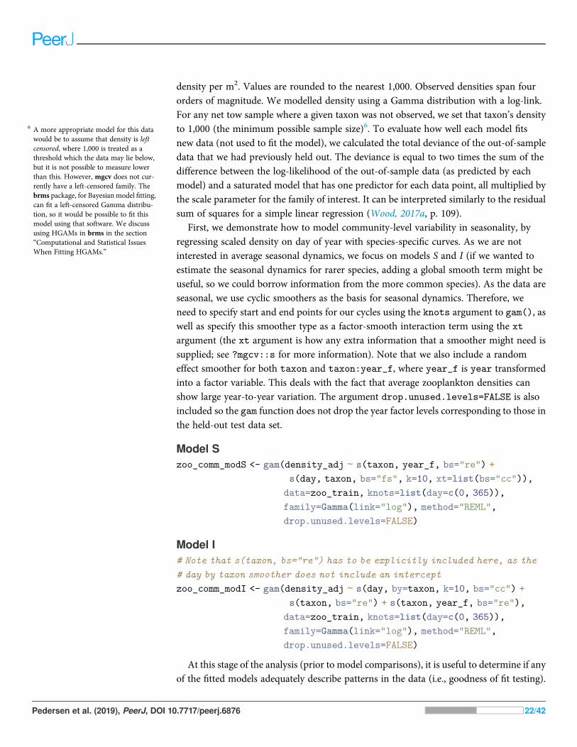
density per m2. Values are rounded to the nearest 1,000. Observed densities span fourorders of magnitude. We modelled density using a Gamma distribution with a log-link.For any net tow sample where a given taxon was not observed, we set that taxon’s densityto 1,000 (the minimum possible sample size)6. To evaluate how well each model fitsnew data (not used to fit the model), we calculated the total deviance of the out-of-sampledata that we had previously held out. The deviance is equal to two times the sum of thedifference between the log-likelihood of the out-of-sample data (as predicted by eachmodel) and a saturated model that has one predictor for each data point, all multiplied bythe scale parameter for the family of interest. It can be interpreted similarly to the residualsum of squares for a simple linear regression (Wood, 2017a, p. 109).

First, we demonstrate how to model community-level variability in seasonality, byregressing scaled density on day of year with species-specific curves. As we are notinterested in average seasonal dynamics, we focus on models S and I (if we wanted toestimate the seasonal dynamics for rarer species, adding a global smooth term might beuseful, so we could borrow information from the more common species). As the data areseasonal, we use cyclic smoothers as the basis for seasonal dynamics. Therefore, weneed to specify start and end points for our cycles using the knots argument to gam(), aswell as specify this smoother type as a factor-smooth interaction term using the xtargument (the xt argument is how any extra information that a smoother might need issupplied; see ?mgcv::s for more information). Note that we also include a randomeffect smoother for both taxon and taxon:year_f, where year_f is year transformedinto a factor variable. This deals with the fact that average zooplankton densities canshow large year-to-year variation. The argument drop.unused.levels=FALSE is alsoincluded so the gam function does not drop the year factor levels corresponding to those inthe held-out test data set.

Model Szoo_comm_modS <- gam(density_adj ∼ s(taxon, year_f, bs="re") +

s(day, taxon, bs="fs", k=10, xt=list(bs="cc")),

data=zoo_train, knots=list(day=c(0, 365)),

family=Gamma(link="log"), method="REML",

drop.unused.levels=FALSE)

Model I# Note that s(taxon, bs="re") has to be explicitly included here, as the

# day by taxon smoother does not include an intercept

zoo_comm_modI <- gam(density_adj ∼ s(day, by=taxon, k=10, bs="cc") +

s(taxon, bs="re") + s(taxon, year_f, bs="re"),

data=zoo_train, knots=list(day=c(0, 365)),



At this stage of the analysis (prior to model comparisons), it is useful to determine if anyof the fitted models adequately describe patterns in the data (i.e., goodness of fit testing).

6 A more appropriate model for this datawould be to assume that density is leftcensored, where 1,000 is treated as athreshold which the data may lie below,but it is not possible to measure lowerthan this. However, mgcv does not cur-rently have a left-censored family. Thebrms package, for Bayesian model fitting,can fit a left-censored Gamma distribu-tion, so it would be possible to fit thismodel using that software. We discussusing HGAMs in brms in the section“Computational and Statistical IssuesWhen Fitting HGAMs.”



https://peerj.com/

mgcv’s gam.check() facilitates this model-checking. This function creates a set ofstandard diagnostic plots: a QQ plot of the deviance residuals (see Wood (2017a))compared to their theoretical expectation for the chosen family, a plot of response vs. fittedvalues, a histogram of residuals, and a plot of residuals vs. fitted values. It also conducts atest for each smooth term to determine if the number of degrees of freedom (k) for eachsmooth is adequate (see ?mgcv::gam.check for details on how that test works). The codefor checking model S and I for the community zooplankton model is:

gam.check(zoo_comm_modS)

gam.check(zoo_comm_modI)

We have plotted QQ plots and fitted-vs. residual plots for model I (fitted vs. response plotsare generally less useful for non-normally distributed data as it can be difficult to visuallyassess if the observed data shows more heteroskedasticity than expected). The resultsfor model S are virtually indistinguishable to the naked eye. We have also used alternateQQ-plotting code from the gratia package (Simpson, 2018), using the qq_plot() function,as this function creates a ggplot2 object that are easier to customize than the base plots fromgam.check(). The code for generating these plots is in the Supplemental Material.These plots (Fig. 14) indicate that the Gamma distribution seems to fit the observed data wellexcept at low values, where the deviance residuals are larger than predicted by the theoreticalquantiles (Fig. 14A). There also does not seem to be a pattern in the residual vs. fittedvalues (Fig. 14B), except for a line of residuals at the lowest values, which correspond to all ofthose observations where a given taxon was absent from the sample.

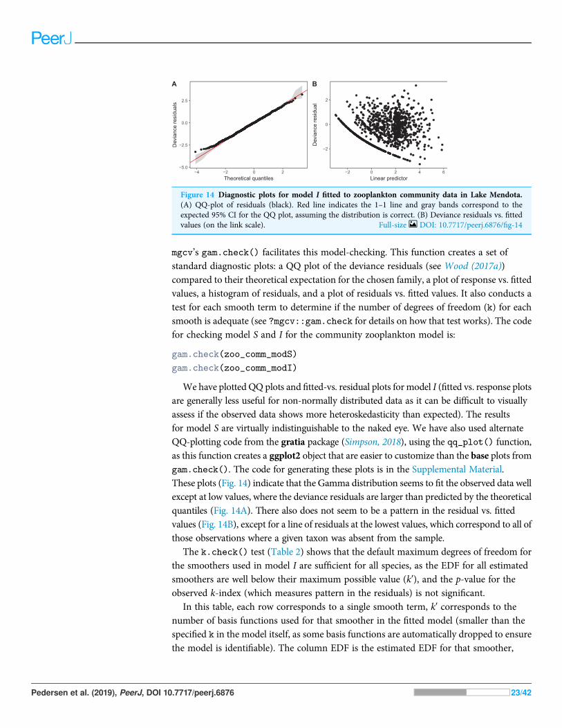
The k.check() test (Table 2) shows that the default maximum degrees of freedom forthe smoothers used in model I are sufficient for all species, as the EDF for all estimatedsmoothers are well below their maximum possible value (k′), and the p-value for theobserved k-index (which measures pattern in the residuals) is not significant.

In this table, each row corresponds to a single smooth term, k′ corresponds to thenumber of basis functions used for that smoother in the fitted model (smaller than thespecified k in the model itself, as some basis functions are automatically dropped to ensurethe model is identifiable). The column EDF is the estimated EDF for that smoother,

−5.0

−2.5

0.0

2.5

−4 −2 0 2Theoretical quantiles

Dev

ianc

e re

sidu

als

A

−2

0

2

−2 0 2 4 6Linear predictor

Dev

ianc

e re

sidu

al

B

Figure 14 Diagnostic plots for model I fitted to zooplankton community data in Lake Mendota.(A) QQ-plot of residuals (black). Red line indicates the 1–1 line and gray bands correspond to theexpected 95% CI for the QQ plot, assuming the distribution is correct. (B) Deviance residuals vs. fittedvalues (on the link scale). Full-size DOI: 10.7717/peerj.6876/fig-14





https://peerj.com/

the k-index is a measure of the remaining pattern in the residuals, and the p-value iscalculated based on the distribution of the k-index after randomizing the order of theresiduals. Note that there is no p-value for the random effects smoothers s(taxon) ands(taxon,year_f) as the p-value is calculated from simulation-based tests forautocorrelation of the residuals. As taxon and year_f are treated as simple random effectswith no natural ordering, there is no meaningful way of checking for autocorrelation.

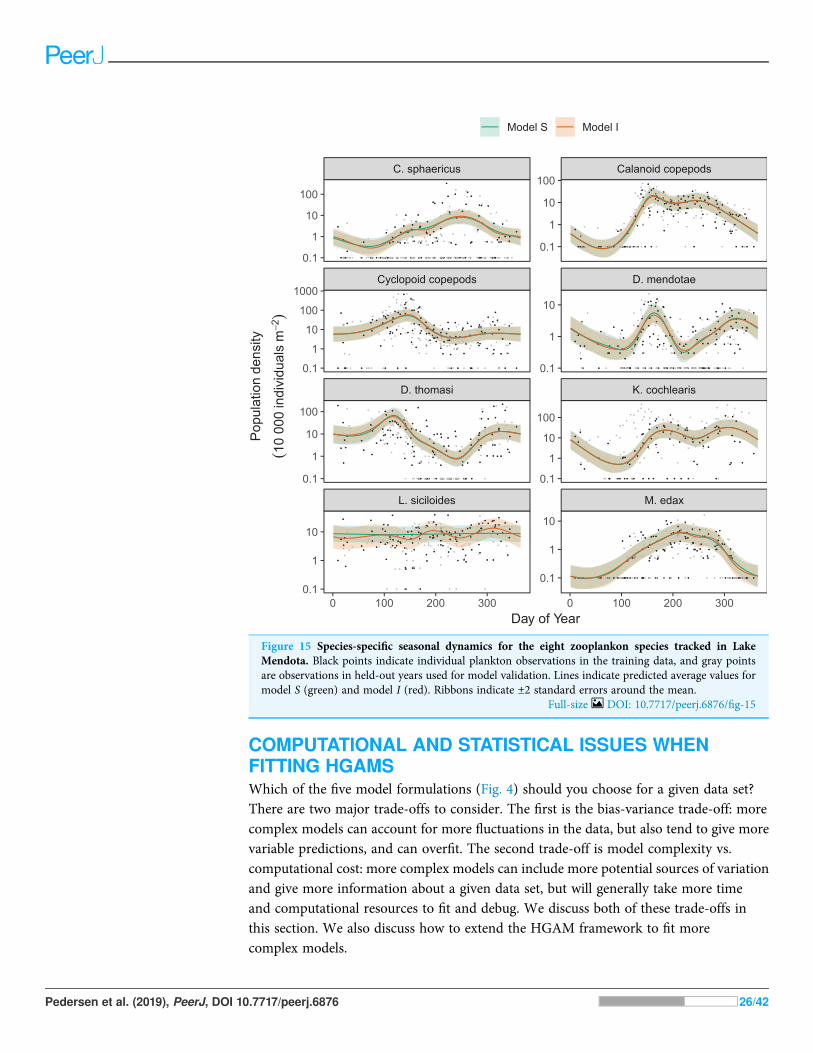
Differences between models S (shared smoothness between taxa) and I (differentsmoothness for each taxa) seem to be driven by the low seasonality of Leptodiaptomussiciloides relative to the other species, and how this is captured by the more flexible modelI (Fig. 15). Still, both models show very similar fits to the training data. This impliesthat the added complexity of different penalties for each species (model I) is unnecessaryhere, which is consistent with the fact that model S has a lower AIC (4667) than model I(4677), and that model S is somewhat better at predicting out-of-sample fits for all taxathan model I (Table 3). Both models show significant predictive improvement comparedto the intercept-only model for all species except Keratella cochlearis (Table 3). This maybe driven by changing timing of the spring bloom for this species between training andout-of-sample years (Fig. 15).

Next, we look at how to fit interlake variability in dynamics for just Daphnia mendotae.Here, we will compare models G, GS, and GI to determine if a single global function isappropriate for all four lakes, or if we can more effectively model variation between lakeswith a shared smoother and lake-specific smoothers.

Model Gzoo_daph_modG <- gam(density_adj ∼ s(day, bs="cc", k=10) + s(lake, bs="re") +

s(lake, year_f, bs="re"),

data=daphnia_train, knots=list(day=c(0, 365)),



Table 2 Results from running k.check() on zoo_comm_modI.

Model term k′ EDF k-index p-value

s(day):taxonC. sphaericus 8 4.78 0.89 0.44

s(day):taxonCalanoid copepods 8 6.66 0.89 0.46

s(day):taxonCyclopoid copepods 8 5.31 0.89 0.46

s(day):taxonD. mendotae 8 6.95 0.89 0.46

s(day):taxonD. thomasi 8 6.57 0.89 0.45

s(day):taxonK. cochlearis 8 5.92 0.89 0.47

s(day):taxonL. siciloides 8 0.52 0.89 0.46

s(day):taxonM. edax 8 4.69 0.89 0.43

s(taxon) 8 6.26 NA NA

s(taxon,year_f) 152 51.73 NA NA

Note:Each row corresponds to a single model term. The notation for term names uses mgcv syntax. For instance, “s(day):taxonC. sphaericus” refers to the smoother for day for the taxon C. sphaericus.



https://peerj.com/

Model GSzoo_daph_modGS <- gam(density_adj ∼ s(day, bs="cc", k=10) +

s(day, lake, k=10, bs="fs", xt=list(bs="cc")) +





Model GIzoo_daph_modGI <- gam(density_adj∼s(day, bs="cc", k=10) +s(lake, bs="re") +

s(day, by=lake, k=10, bs="cc") +



family=Gamma(link ="log"), method="REML",


Diagnostic plots from gam.check() indicate that there are no substantial patternscomparing residuals to fitted values (not shown), and QQ-plots are similar to those fromthe zooplankton community models; the residuals for all three models closely correspondto the expected (Gamma) distribution, except at small values, where the observedresiduals are generally larger than expected (Fig. 16). As with the community data, this islikely an artifact of the assumption we made of assigning zero observations a value of 1,000(the lowest possible value), imposing an artificial lower bound on the observed counts.There was also some evidence that the largest observed values were smaller than expectedgiven the theoretical distribution, but these fell within the 95% CI for expected deviationsfrom the 1–1 line (Fig. 16).

AIC values indicate that both model GS (1,093.71) and GI (1,085.7) are better fits thanmodel G (1,097.62), with model GI fitting somewhat better than model GS.7 There doesnot seem to be a large amount of interlake variability (the EDF per lake are low inmodels GS & GI). Plots for all three models (Fig. 17) show that Mendota, Monona, andKegonsa lakes are very close to the average and to one another for both models, butWaubesashows evidence of a more pronounced spring bloom and lower winter abundances.

Model GI is able to predict as well or better than model G or GS for all lakes (Table 4),indicating that allowing for interlake variation in seasonal dynamics improved modelprediction. All three models predicted dynamics in Lake Mendota and Lake Menonasignificantly better than the intercept-only model (Table 4). None of the models did well interms of predicting Lake Waubesa dynamics out-of-sample compared to a simple modelwith only a lake-specific intercept and no intra-annual variability, but this was due tothe influence of a single large outlier in the out-of-sample data that occurred after thespring bloom, at day 243 (Fig. 17; note that the y-axis is log-scaled). However, baring amore detailed investigation into the cause of this large value, we cannot arbitrarily excludethis outlier from the goodness-of-fit analysis; it may be due either to measurement error ora true high late-season Daphnia density that our model was not able to predict.

7 When comparing models via AIC, we usethe standard rule of thumb fromBurnham & Anderson (1998), wheremodels that differ by two units or lessfrom the lowest AIC model have sub-stantial support, and those differing bymore than four units have less support.



https://peerj.com/

COMPUTATIONAL AND STATISTICAL ISSUES WHENFITTING HGAMSWhich of the five model formulations (Fig. 4) should you choose for a given data set?There are two major trade-offs to consider. The first is the bias-variance trade-off: morecomplex models can account for more fluctuations in the data, but also tend to give morevariable predictions, and can overfit. The second trade-off is model complexity vs.computational cost: more complex models can include more potential sources of variationand give more information about a given data set, but will generally take more timeand computational resources to fit and debug. We discuss both of these trade-offs inthis section. We also discuss how to extend the HGAM framework to fit morecomplex models.

L. siciloides M. edax

D. thomasi K. cochlearis

Cyclopoid copepods D. mendotae

C. sphaericus Calanoid copepods

0 100 200 300 0 100 200 300

0.1

1

10

100

0.1

1

10

0.1

1

10

100

0.1

1

10

0.1

1

10

100

0.1

1

10

100

1000

0.1

1

10

100

0.1

1

10

Day of Year

Pop

ulat

ion

dens

ity

(10

000

indi

vidu

als

m−2

)

Model S Model I

Figure 15 Species-specific seasonal dynamics for the eight zooplankon species tracked in LakeMendota. Black points indicate individual plankton observations in the training data, and gray pointsare observations in held-out years used for model validation. Lines indicate predicted average values formodel S (green) and model I (red). Ribbons indicate ±2 standard errors around the mean.





https://peerj.com/

Bias-variance trade-offsThe bias-variance trade-off is a fundamental concept in statistics. When trying to estimateany relationship (in the case of GAMs, a smooth relationship between predictors and data)bias measures how far, on average, an estimate is from the true value. The variance ofan estimator corresponds to how much that estimator would fluctuate if applied to multipledifferent samples of the same size taken from the same population. These two propertiestend to be traded off when fitting models. For instance, rather than estimating a populationmean from data, we could simply use a predetermined fixed value regardless of the observeddata8. This estimate would have no variance (as it is always the same regardless of whatthe data look like) but would have high bias unless the true population mean happened toequal the fixed value we chose. Penalization is useful because using a penalty term slightlyincreases model bias, but can substantially decrease variance (Efron & Morris, 1977).

In GAMs, the bias-variance trade-off is managed by the terms of the penalty matrix, andequivalently random effect variances in HGLMs. Larger penalties correspond to lower

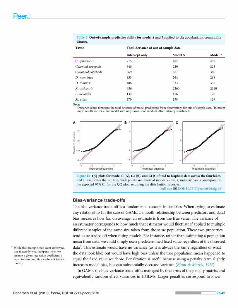
Table 3 Out-of-sample predictive ability for model S and I applied to the zooplankton communitydataset.

Taxon Total deviance of out-of-sample data

Intercept only Model S Model I

C. sphaericus 715 482 495

Calanoid copepods 346 220 223

Cyclopoid copepods 569 381 386

D. mendotae 353 264 268

D. thomasi 486 333 337

K. cochlearis 486 2260 2340

L. siciloides 132 116 126

M. edax 270 138 139

Note:Deviance values represent the total deviance of model predictions from observations for out-of-sample data. “Interceptonly” results are for a null model with only taxon-level random effect intercepts included.

−4

−2

0

2


Dev

ianc

e re

sidu

als

−4

−2

0

2

4


−4

−2

0

2

−2 0 2Theoretical quantiles

A B C

Figure 16 QQ-plots for model G (A), GS (B), and GI (C) fitted to Daphnia data across the four lakes.Red line indicates the 1-1 line, black points are observed model residuals, and gray bands correspond tothe expected 95% CI for the QQ plot, assuming the distribution is correct.


8 While this example may seem contrived,this is exactly what happens when weassume a given regression coefficient isequal to zero (and thus exclude it from amodel).




https://peerj.com/

variance, as the estimated function is unable to wiggle a great deal, but also correspond tohigher bias unless the true function is close to the null space for a given smoother (e.g., astraight line for TPRS with second derivative penalties, or zero for a random effect). Thecomputational machinery used by mgcv to fit smooth terms is designed to find penaltyterms that best trade-off bias for variance to find a smoother that can effectively predictnew data.

The bias-variance trade-off comes into play with HGAMs when choosing whether to fitseparate penalties for each group level or assign a common penalty for all group levels (i.e.,deciding between models GS & GI or models S & I). If the functional relationships we are

Menona Waubesa

Kegonsa Mendota

100 200 300 100 200 300

0.1

1.0

10.0

0.1

1.0

10.0

Day of Year

Pop

ulat

ion

dens

ity

(10

000

indi

vidu

als

m−2

)

Model G Model GS Model GI

Figure 17 Raw data (points) and fitted models (lines) for D. mendota data. Black points indicateindividual plankton observations in the training data, and gray points are observations in held-out yearsused for model validation. Green line: model G (no inter-lake variation in dynamics); orange line: modelGS (interlake variation with similar smoothness); purple line: model GI (varying smoothness amonglakes). Shaded bands are drawn at ±2 standard errors around each model.


Table 4 Out-of-sample predictive ability for modelG,GS, andGI applied to theD. mendotae dataset.

Lake Total deviance of out-of-sample data

Intercept only Model G Model GS Model GI

Kegonsa 96 92 89 86

Mendota 352 258 257 257

Menona 348 300 294 290

Waubesa 113 176 164 157

Note:Deviance values represent the total deviance of model predictions from observations for out-of-sample data. “Interceptonly” results are for a null model with only lake-level random effect intercepts included.




https://peerj.com/

trying to estimate for different group levels actually vary in how wiggly they are, setting thepenalty for all group-level smoothers equal (models GS & S) will either lead to overlyvariable estimates for the least variable group levels, over-smoothed (biased) estimates forthe most wiggly terms, or a mixture of these two, depending on the fitting criteria.

We developed a simple numerical experiment to determine whether mgcv’s fittingcriteria tend to set estimated smoothness penalties high or low in the presence of among-group variability in smoothness when fitting model GS or S HGAMs. We simulateddata from four different groups, with all groups having the same levels of the covariate x,equally spaced across the range from 0 to 2π. For each group, the true function relating x tothe response, y, was a cosine wave, but the frequency varied from 0.5 (equal to half acycle across the range of x) to 4 (corresponding to 4 full cycles across the range). As all foursine waves spanned the whole range from -1 to +1 across the range of x, and as they wereall integer or half-integer frequencies, the signal for all groups had the same varianceacross the range of x, approximately equal to 0.5. Therefore, the true function for all groupshad the same strength of signal; all that varied between groups was how rapidly the signalfluctuated. We added normally distributed error to all y-values, with three differentnoise levels, given by standard deviations of 0.5, 1, and 2. These correspond to signal-to-noise ratios (i.e., variance of the cosine curve divided by variance of the noise) of 2,0.5, and 0.125. For each noise level we created 25 replicate data sets to illustrate the amountof simulation-to-simulation variation in model fit. We then fit both model S (where allcurves were assumed to be equally smooth) and model I (with varying smoothness) toeach replicate for each noise level, using REML criteria to estimate penalties.

A sample of the fits for each group for three of the replicates for each model are shownin Fig. 18A, with model S in red and model I in blue. Figure 18B illustrates how well eachmodel fared across the range of replicates at accurately estimating the true smoothnessof the highest frequency terms as measured by the squared second derivative of the smoothfit vs. that of the true function, with the distance to the black one-to-one line indicatingthe degree to which the estimated function for each group over- or under-estimatedthe smoothness of the true signal. In general, under low noise conditions (Fig. 18,signal-to-noise ratio of 2), model S tended to overfit the smoothest, lowest-frequency,groups, while accurately fitting the highest frequency groups. Under moderate signal-to-noise ratios, model S tended to over-penalize high-frequency groups and under-penalizelow frequency groups, and in the lowest signal-to-noise ratio tested (0.125), model Stended to penalize all groups toward very smooth functions (Fig. 18B). Curves estimatedby model I, on the other hand, tended to accurately capture the true wiggliness of thefunction across the whole range of frequencies and noises, except for the lowest-frequencygroups, and the highest frequency groups it the presence of high noise; in both cases,model I tended to over-smooth (Fig. 18B).

This implies that assuming equal smoothness will result in underestimating the truesmoothness of low-variability terms in cases of high signal-to-noise, and overestimatingthe true smoothness of high-frequency terms in low signal-to-noise data sets. If thisis a potential issue, we recommend fitting both models S and I and using standard modelevaluation criteria (e.g., AIC) or out-of-sample predictive accuracy (as in the section



https://peerj.com/

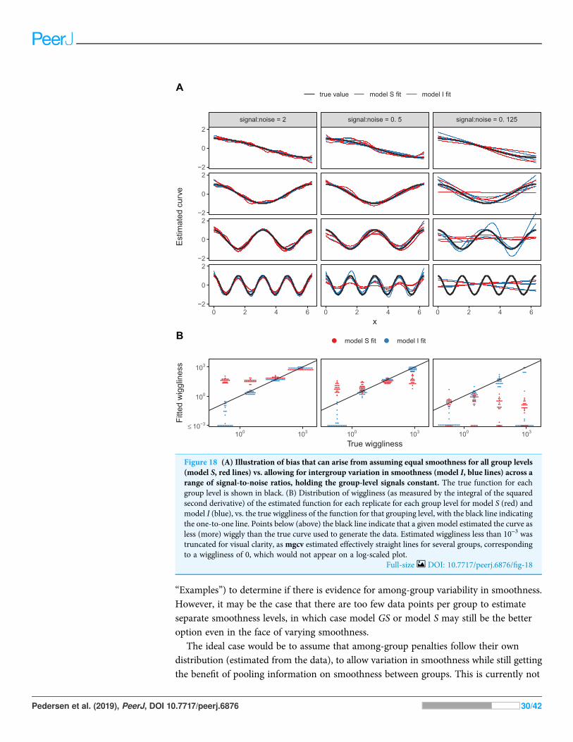
“Examples”) to determine if there is evidence for among-group variability in smoothness.However, it may be the case that there are too few data points per group to estimateseparate smoothness levels, in which case model GS or model S may still be the betteroption even in the face of varying smoothness.

The ideal case would be to assume that among-group penalties follow their owndistribution (estimated from the data), to allow variation in smoothness while still gettingthe benefit of pooling information on smoothness between groups. This is currently not

signal:noise = 2 signal:noise = 0. 5 signal:noise = 0. 125

0 2 4 6 0 2 4 6 0 2 4 6

−2

0

2

−2

0

2

−2

0

2

−2

0

2

x

Est

imat

ed c

urve

true value model S fit model I fit

100 103 100 103 100 103≤ 10−3

100

103

True wiggliness

Fitte

d w

iggl

ines

s

model S fit model I fit

A

B

Figure 18 (A) Illustration of bias that can arise from assuming equal smoothness for all group levels(model S, red lines) vs. allowing for intergroup variation in smoothness (model I, blue lines) across arange of signal-to-noise ratios, holding the group-level signals constant. The true function for eachgroup level is shown in black. (B) Distribution of wiggliness (as measured by the integral of the squaredsecond derivative) of the estimated function for each replicate for each group level for model S (red) andmodel I (blue), vs. the true wiggliness of the function for that grouping level, with the black line indicatingthe one-to-one line. Points below (above) the black line indicate that a given model estimated the curve asless (more) wiggly than the true curve used to generate the data. Estimated wiggliness less than 10-3 wastruncated for visual clarity, as mgcv estimated effectively straight lines for several groups, correspondingto a wiggliness of 0, which would not appear on a log-scaled plot.





https://peerj.com/

implemented in mgcv. It is possible to set up this type of varying penalty model inflexible Bayesian modeling software such as Stan (see below for a discussion of how to fitHGAMs using these tools), where intergroup variation in smoothing penalties couldbe modelled with a hierarchical prior. However, to the best of our knowledge, how to fit thistype of model has not been well studied in either the Bayesian or frequentist literature.

It may seem there is also a bias-variance trade-off between choosing to use a singleglobal smoother (model G) or a global smoother plus group-level terms (models GS andGI). In model G, all the data is used to estimate a single smooth term, and thus shouldhave lower variance than models GS and GI, but higher bias for any given group inthe presence of intergroup functional variability. However, in practice, this trade-off will behandled via penalization; if there are no average differences between functional responses,mgcv will penalize the group-specific functions toward zero, and thus toward theglobal model. The choice between using model G vs. models GS and GI should generally bedriven by computational costs. Model G is typically much faster to fit than models GS andGI, even in the absence of among-group differences. If there is no need to estimateintergroup variability, model G will typically be more efficient.

A similar issue exists when choosing between models GS and GI and models S and I.If all group levels have very different functional shapes, the global term will get penalizedtoward zero in models GS and GI, so they will reduce to models S and I. The choiceto include a global term should be made based on scientific considerations (is the globalterm of interest?) and computational considerations.

Complexity-computation trade-offsThe more flexible a model is, the larger an effective parameter space any fitting softwarehas to search. It can be surprisingly easy to use massive computational resources tryingto fit models to even small datasets. While we typically want to select models based ontheir fit and our inferential goals, computing resources can often act as an effective upperbound on model complexity. For a given data set, assuming a fixed family and linkfunction, the time taken to estimate an HGAM will depend (roughly) on four factors:(i) the number of coefficients to be estimated (and thus the number of basis functionschosen), (ii) the number of smoothing parameters to be estimated, (iii) whether the modelneeds to estimate both a global smoother and group-level smoothers, and (iv) thealgorithm and fitting criteria used to estimate parameters.

The most straightforward factor that will affect the amount of computational resources isthe number of parameters in the model. Adding group-level smoothers (moving frommodelG to the other models) means that there will be more regression parameters to estimate.For a dataset with g different groups and n data points, fitting a model with just a globalsmoother, y∼s(x,k=k) will require k coefficients, and takes Oðnk2Þ operations to evaluate.Fitting the same data using a group-level smoother (model S, y∼s(x,fac,bs="fs",k=k))will require Oðnk2g2Þ operations to evaluate. In effect, adding a group-level smootherwill increase computational cost by an order of the number of groups squared. The effect ofthis is visible in the examples we fit in the section “What are Hierarchical GAMs?.” Table 5compares the relative time it takes to compute model G vs. the other models.



https://peerj.com/

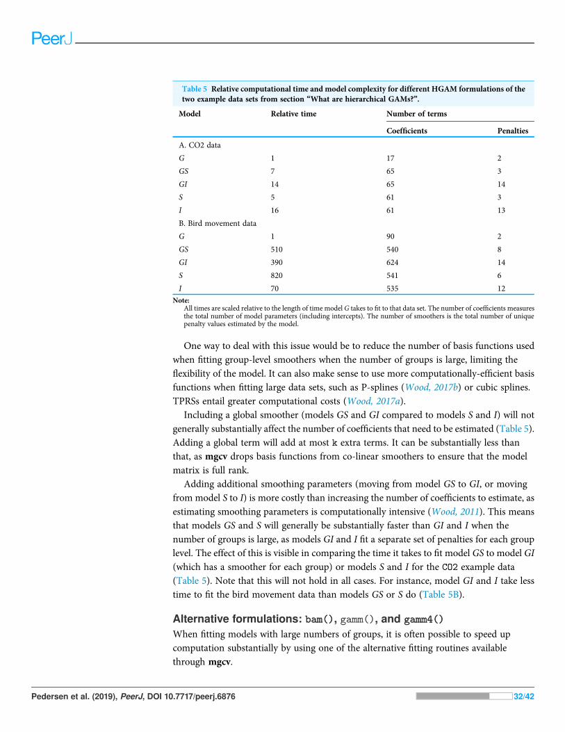
One way to deal with this issue would be to reduce the number of basis functions usedwhen fitting group-level smoothers when the number of groups is large, limiting theflexibility of the model. It can also make sense to use more computationally-efficient basisfunctions when fitting large data sets, such as P-splines (Wood, 2017b) or cubic splines.TPRSs entail greater computational costs (Wood, 2017a).

Including a global smoother (models GS and GI compared to models S and I) will notgenerally substantially affect the number of coefficients that need to be estimated (Table 5).Adding a global term will add at most k extra terms. It can be substantially less thanthat, as mgcv drops basis functions from co-linear smoothers to ensure that the modelmatrix is full rank.

Adding additional smoothing parameters (moving from model GS to GI, or movingfrom model S to I) is more costly than increasing the number of coefficients to estimate, asestimating smoothing parameters is computationally intensive (Wood, 2011). This meansthat models GS and S will generally be substantially faster than GI and I when thenumber of groups is large, as models GI and I fit a separate set of penalties for each grouplevel. The effect of this is visible in comparing the time it takes to fit model GS to model GI(which has a smoother for each group) or models S and I for the CO2 example data(Table 5). Note that this will not hold in all cases. For instance, model GI and I take lesstime to fit the bird movement data than models GS or S do (Table 5B).

Alternative formulations: bam()bam(), gamm(), and gamm4()gamm4()

When fitting models with large numbers of groups, it is often possible to speed upcomputation substantially by using one of the alternative fitting routines availablethrough mgcv.

Table 5 Relative computational time and model complexity for different HGAM formulations of thetwo example data sets from section “What are hierarchical GAMs?”.

Model Relative time Number of terms

Coefficients Penalties

A. CO2 data

G 1 17 2

GS 7 65 3

GI 14 65 14

S 5 61 3

I 16 61 13

B. Bird movement data

G 1 90 2

GS 510 540 8

GI 390 624 14

S 820 541 6

I 70 535 12

Note:All times are scaled relative to the length of time model G takes to fit to that data set. The number of coefficients measuresthe total number of model parameters (including intercepts). The number of smoothers is the total number of uniquepenalty values estimated by the model.



https://peerj.com/

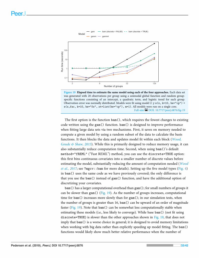
The first option is the function bam(), which requires the fewest changes to existingcode written using the gam() function. bam() is designed to improve performancewhen fitting large data sets via two mechanisms. First, it saves on memory needed tocompute a given model by using a random subset of the data to calculate the basisfunctions. It then blocks the data and updates model fit within each block (Wood,Goude & Shaw, 2015). While this is primarily designed to reduce memory usage, it canalso substantially reduce computation time. Second, when using bam()’s defaultmethod="fREML" (“Fast REML”) method, you can use the discrete=TRUE option:this first bins continuous covariates into a smaller number of discrete values beforeestimating the model, substantially reducing the amount of computation needed (Woodet al., 2017; see ?mgcv::bam for more details). Setting up the five model types (Fig. 4)in bam() uses the same code as we have previously covered; the only difference isthat you use the bam() instead of gam() function, and have the additional option ofdiscretizing your covariates.

bam() has a larger computational overhead than gam(); for small numbers of groups itcan be slower than gam() (Fig. 19). As the number of groups increases, computationaltime for bam() increases more slowly than for gam(); in our simulation tests, whenthe number of groups is greater than 16, bam() can be upward of an order of magnitudefaster (Fig. 19). Note that bam() can be somewhat less computationally stable whenestimating these models (i.e., less likely to converge). While base bam() (not fit usingdiscrete=TRUE) is slower than the other approaches shown in Fig. 19, that does notimply that bam() is a worse choice in general; it is designed to avoid memory limitationswhen working with big data rather than explicitly speeding up model fitting. The bam()functions would likely show much better relative performance when the number of

0.1

1

10

100

2 8 32 128Number of groups

Run

tim

e (s

econ

ds)

Modelgam bam (discrete = FALSE) bam (discrete = TRUE)

gamm gamm4

Figure 19 Elapsed time to estimate the same model using each of the four approaches. Each data setwas generated with 20 observations per group using a unimodal global function and random group-specific functions consisting of an intercept, a quadratic term, and logistic trend for each group.Observation error was normally distributed. Models were fit using model 2: y s(x, k=10, bs="cp") +

s(x,fac, k=10, bs="fs", xt=list(bs="cp"), m=1). All models were run on a single core.Full-size DOI: 10.7717/peerj.6876/fig-19




https://peerj.com/

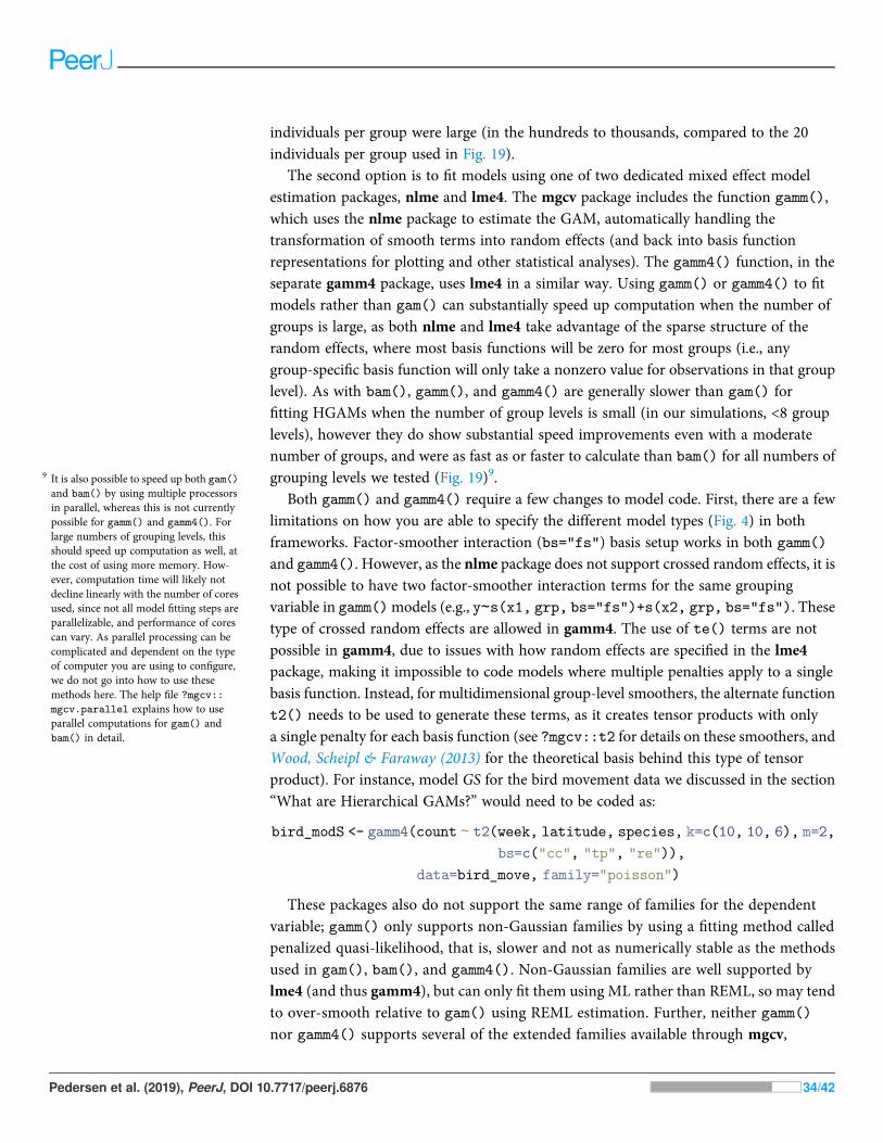
individuals per group were large (in the hundreds to thousands, compared to the 20individuals per group used in Fig. 19).

The second option is to fit models using one of two dedicated mixed effect modelestimation packages, nlme and lme4. The mgcv package includes the function gamm(),which uses the nlme package to estimate the GAM, automatically handling thetransformation of smooth terms into random effects (and back into basis functionrepresentations for plotting and other statistical analyses). The gamm4() function, in theseparate gamm4 package, uses lme4 in a similar way. Using gamm() or gamm4() to fitmodels rather than gam() can substantially speed up computation when the number ofgroups is large, as both nlme and lme4 take advantage of the sparse structure of therandom effects, where most basis functions will be zero for most groups (i.e., anygroup-specific basis function will only take a nonzero value for observations in that grouplevel). As with bam(), gamm(), and gamm4() are generally slower than gam() forfitting HGAMs when the number of group levels is small (in our simulations, <8 grouplevels), however they do show substantial speed improvements even with a moderatenumber of groups, and were as fast as or faster to calculate than bam() for all numbers ofgrouping levels we tested (Fig. 19)9.

Both gamm() and gamm4() require a few changes to model code. First, there are a fewlimitations on how you are able to specify the different model types (Fig. 4) in bothframeworks. Factor-smoother interaction (bs="fs") basis setup works in both gamm()

and gamm4(). However, as the nlme package does not support crossed random effects, it isnot possible to have two factor-smoother interaction terms for the same groupingvariable in gamm()models (e.g., y∼s(x1, grp, bs="fs")+s(x2, grp, bs="fs"). Thesetype of crossed random effects are allowed in gamm4. The use of te() terms are notpossible in gamm4, due to issues with how random effects are specified in the lme4package, making it impossible to code models where multiple penalties apply to a singlebasis function. Instead, for multidimensional group-level smoothers, the alternate functiont2() needs to be used to generate these terms, as it creates tensor products with onlya single penalty for each basis function (see ?mgcv::t2 for details on these smoothers, andWood, Scheipl & Faraway (2013) for the theoretical basis behind this type of tensorproduct). For instance, model GS for the bird movement data we discussed in the section“What are Hierarchical GAMs?” would need to be coded as:

bird_modS <- gamm4(count ∼ t2(week, latitude, species, k=c(10, 10, 6), m=2,

bs=c("cc", "tp", "re")),

data=bird_move, family="poisson")

These packages also do not support the same range of families for the dependentvariable; gamm() only supports non-Gaussian families by using a fitting method calledpenalized quasi-likelihood, that is, slower and not as numerically stable as the methodsused in gam(), bam(), and gamm4(). Non-Gaussian families are well supported bylme4 (and thus gamm4), but can only fit them using ML rather than REML, so may tendto over-smooth relative to gam() using REML estimation. Further, neither gamm()nor gamm4() supports several of the extended families available through mgcv,

9 It is also possible to speed up both gam()

and bam() by using multiple processorsin parallel, whereas this is not currentlypossible for gamm() and gamm4(). Forlarge numbers of grouping levels, thisshould speed up computation as well, atthe cost of using more memory. How-ever, computation time will likely notdecline linearly with the number of coresused, since not all model fitting steps areparallelizable, and performance of corescan vary. As parallel processing can becomplicated and dependent on the typeof computer you are using to configure,we do not go into how to use thesemethods here. The help file ?mgcv::mgcv.parallel explains how to useparallel computations for gam() andbam() in detail.



https://peerj.com/

such as zero-inflated, negative binomial, or ordered categorical and multinomialdistributions.

Estimation issues when fitting both global and group-level smoothersWhen fitting models with separate global and group-level smoothers (models GS and GI),one issue to be aware of is concurvity between the global smoother and group-levelterms. Concurvity measures how well one smooth term can be approximated by somecombination of the other smooth terms in the model (see ?mgcv::concurvity fordetails). For models GS and GI, the global term is either entirely or almost entirely10

concurved with the group-level smoothers. This is because, in the absence of the globalsmooth term, it would be possible to recreate that average effect by shifting all thegroup-level smoothers so they were centered around the global mean.

In practical terms, this has the consequence of increasing uncertainty around the globalmean relative to a model with only a global smoother. In some cases, it can result inthe estimated global smoother being close to flat, even in simulated examples with aknown strong global effect. This concurvity issue may also increase the time it takes tofit these models (e.g., compare the time it takes to fit models GI and I in Table 5).These models can still be estimated because of penalty terms; all of the methods we havediscussed for fitting model GS (factor-smoother terms or random effect tensor products)automatically create a penalty for the null space of the group-level terms, so that onlythe global term has its own unpenalized null space. Both the REML and ML criteria workto balance penalties between nested smooth terms (this is why nested random effectscan be fitted). We have observed thatmgcv still occasionally finds solutions with simulateddata where the global term is over-smoothed.

To avoid this issue, we recommend both careful choice of basis and relative degrees offreedom of global and group-level terms. In the examples in section “What areHierarchical GAMs?,” we used smoothers with an unpenalized null space for the globalsmoother and ones with no null space for the group-level terms. When using TPRS thiscan be achieved with splines with a lower order of derivative penalized in the group-levelsmoothers than the global smoothers, as lower-order TPRS have fewer basis functionsin the null space. For example, we used m=2 (penalizing squared second derivatives) forthe global smoother, and m=1 (penalizing squared first derivatives) for group-levelsmoothers in models GS and GI. Another option is to specify the maximum degrees offreedom (k) for the group-level smoother either substantially higher or lower than theglobal smoother; this is in effect an approximate way to specify a prior belief in the relativesmoothness of the global vs. group-level functions. If the group-level term is set tohave greater k compared to the global term, this encodes the assumption that the globalfunction should not be very wiggly, but group-level deviations from that smooth mightvary from that, and vice versa if k is set lower for group-level terms than for theglobal smoother.

As noted above, interpreting the shape of global terms and group-wise deviationsseparately for GS models fit using tensor-product group-level terms is complicated by thefact that mgcv will drop some basis-functions from the group-level terms to prevent

10 There is an important caveat here.When fitting GS models using tensorproducts inmgcv, the global and group-level terms will not be entirely concurvebecause mgcv will automatically dropbasis functions from the group-levelsmoother to ensure that these terms arenot perfectly concurve. That is, so thatno basis function in the global termcould be formed from a linear combi-nation of group-level basis functions(see ?mgcv::gam.side for how termsto be dropped are selected). Group-levelterms fit using bs="fs" smoothers willnot have any basis functions dropped, asmgcv disables checking for side-con-straints for these smoothers (since allbasis functions are fully penalized forthis type of smoother, in principle con-curvity should not be an issue; see?mgcv::smooth.construct.fs.

smooth.spec for details).



https://peerj.com/

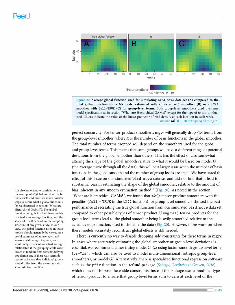
perfect concurvity. For tensor-product smoothers,mgcv will generally drop �K terms fromthe group-level smoother, where K is the number of basis functions in the global smoother.The total number of terms dropped will depend on the smoothers used for the globaland group-level terms. This means that some groups will have a different range of potentialdeviations from the global smoother than others. This has the effect of also somewhataltering the shape of the global smooth relative to what it would be based on model G(the average curve through all the data); this will be a larger issue when the number of basisfunctions in the global smooth and the number of group levels are small. We have tested theeffect of this issue on our simulated bird_move data set and did not find that it lead tosubstantial bias in estimating the shape of the global smoother, relative to the amount ofbias inherent in any smooth estimation method11 (Fig. 20). As noted in the section“What are hierarchical GAMs?”, we found that t2() tensor product smoothers with fullpenalties (full = TRUE in the t2() function) for group-level smoothers showed the bestperformance at recreating the true global function from our simulated bird_move data set,compared to other possible types of tensor product. Using te() tensor products for thegroup-level terms lead to the global smoother being heavily smoothed relative to theactual average function, used to simulate the data (Fig. 20). However, more work on whenthese models accurately reconstruct global effects is still needed.

There is currently no way to disable dropping side constraints for these terms in mgcv.In cases where accurately estimating the global smoother or group-level deviations isessential, we recommend either fitting model G, GS using factor-smooth group-level terms(bs="fs", which can also be used to model multi-dimensional isotropic group-levelsmoothers), or model GI. Alternatively, there is specialized functional regression softwaresuch as the pffr function in the refund package (Scheipl, Gertheiss & Greven, 2016),which does not impose these side constraints; instead the package uses a modified typeof tensor-product to ensure that group-level terms sum to zero at each level of the

true global function te t2

0 10 20 30 40 50 0 10 20 30 40 50 0 10 20 30 40 50

20

40

60

weekla

titud

e

−30 −20 −10 0 10linear predictor

A B C

Figure 20 Average global function used for simulating bird_move data set (A) compared to thefitted global function for a GS model estimated with either a te() smoother (B) or a t2()

smoother with full=TRUE (C) for group-level terms. Both group-level smoothers used the samemodel specification as in section “What are Hierarchical GAMs?” except for the type of tensor productused. Colors indicate the value of the linear predictor of bird density at each location in each week.


11 It is also important to consider here thatthe concept of a “global function” is a bitfuzzy itself, and there are many possibleways to define what a global function is(as we discussed in section “What areHierarchical GAMs?”). The globalfunction being fit in all of these modelsis actually an average function, and theshape of it will depend on the samplingstructure of any given study. In ourview, the global function fitted in thesemodels should generally be viewed as auseful summary of an average trendacross a wide range of groups, andwould only represent an actual averagerelationship if the grouping levels weredrawn at random from some underlyingpopulation and if there was scientificreason to believe that individual groupsshould differ from the mean only viasome additive function.




https://peerj.com/

predictor (Scheipl, Gertheiss & Greven, 2016). See below for more information onfunctional regression.

A brief foray into the land of BayesAsmentioned in the section “A Review of Generalized Additive Models,” the penalty matrixcan be interpreted as the prior precision (inverse prior covariance) matrix for the modelparameters β. Intuitively, the basis functions and penalty are an informal prior on how we’dlike our model term to behave. REML gives an empirical Bayes estimate of the smoothmodel (Laird &Ware, 1982), where terms in the null space of the smoother have improper,flat priors (i.e., any value for these terms are considered equally likely). Any terms in therange space are treated as having a multivariate normal prior, and the smoothingparameters are treated as having an improper flat prior (see Wood (2017a), Section 5.8 formore details on this connection). The posterior covariance matrix (Wood, 2006b) formodel parameters can be extracted from any fitted gam() or bam() model with vcov

(model) (this is conditional on the estimated smoothing parameters unless the optionunconditional=TRUE is specified). Given the normal posterior for the estimates of β, wecan sample from a multivariate normal with mean β̂ and posterior covariance matrix. Suchsamples can be used to estimate uncertainty in functions of the predictors. Viewing ourGAM as Bayesian is a somewhat unavoidable consequence of the equivalence of randomeffects and splines—if we think that there is some true smoother that we wish to estimate,we must take a Bayesian view of our random effects (splines) as we do not think thatthe true smoother changes each time we collect data (Wood, 2017a, Section 5.8).The standard confidence intervals used in mgcv are in fact Bayesian posterior credibleintervals, which happen to have good frequentist across-the-function properties (Wood,2006b;Marra &Wood, 2012). The newest version ofmgcv as of this writing (v. 1.8–28) alsoincludes an experimental implementation of integrated nested Laplace approximation tocalculate full posterior distributions for GAMs, via the ginla function (Wood, in press).

This also means that HGAMs can be included as components in a more complex fullyBayesian model. The mgcv package includes a function jagam() that can take a specifiedmodel formula and automatically convert it into code for the JAGS (or BUGS) Bayesianstatistical packages, which can be adapted by the user to their own needs.

Similarly, the brms package (Bürkner, 2017), which can fit complex statistical modelsusing the Bayesian software Stan (Carpenter et al., 2017) allows for the inclusion ofmgcv-style smooth terms as part of the model specification. The brms package does notcurrently support te() tensor products, but does support factor-smooth interactionsand t2()-style tensor products, which means all of the models fitted in this paper can befitted by brms. Finally, the bamlss package (Umlauf, Klein & Zeileis, 2018) can fit complexGAMs using a number of computational backends, including JAGS and BayesX, usingmgcv syntax for model specification.

Beyond HGAMs: functional regressionThe HGAMs we have discussed are actually a type of functional regression, which is anextension of standard regression models to cases where the outcome variable yi and/or the



https://peerj.com/

predictor variables xi for a given outcome are functions, rather than single variables(Ramsay & Silverman, 2005). HGAMs as we have described them are a form of function-on-scalar regression (Ramsay & Silverman, 2005; Reiss, Huang & Mennes, 2010), wherewe are trying to estimate a smooth function that varies between grouping levels. Here the“scalar” refers to the grouping level, and the function is the smooth term that variesbetween levels; in contrast, a standard GAM is a type of scalar-on-scalar regression,as the goal is to use a set of single values (scalars) to estimate each (scalar) response.

We have deliberately focused our paper on these simpler classes of functional regressionmodel, and chosen to use the term HGAM rather than functional regression, as we believethat this more clearly connects these models to modeling approaches already familiarto ecologists. Further, we consider the unit of analysis to still be individual observations,as compared to functional regression where the unit of analysis is whole functions.For instance, we are interested in applications such as species distribution modeling, wherethe presence of a given species may be predicted from a sum of several species-specificfunctions of different environmental variables.

However, there is an extensive literature dedicated to the estimation of more complexfunctional regression models for any interested reader (seeMorris (2015) andGreven & Scheipl(2017) for a good introduction and overview of more recent work in this field). Therefund package (Greven & Scheipl, 2017) uses the statistical machinery of mgcv to fit thesemodels, and should be usable by anyone familiar with mgcv modeling syntax. Functionalregression is also a major area of study in Bayesian statistics (Kaufman & Sain, 2010).

CONCLUSIONHierarchical GAMs are a powerful tool to model intergroup variability, and we haveattempted to illustrate some of the range and possibilities that these models are capable of,how to fit them, and some issues that may arise during model fitting and testing. Specifyingthese models and techniques for fitting them are active areas statistical research,so this paper should be viewed as a jumping-off point for these models, rather than anend-point; we refer the reader to the rich literature on GAMs (Wood, 2017a) andfunctional regression (Ramsay & Silverman, 2005; Kaufman & Sain, 2010; Scheipl,Staicu & Greven, 2014) for more on these ideas.

ACKNOWLEDGEMENTSThe authors would like to thank Carly Ziter, Tiago Marques, Jake Walsh, Geoff Evans,Paul Regular, Laura Wheeland, and Isabella Ghement for their thoughtful feedback onearlier versions of this manuscript, and the Ecological Society of America for hostingthe mgcv workshops that this work started from. The authors also thank the threereviewers (Paul Bürkner, Fabian Scheipl, and Matteo Fasiolo) for their insightful anduseful feedback.

All authors contributed to developing the initial idea for this paper, and to writing andediting the manuscript. Author order after the first author was chosen using the code:

set.seed(11)

sample(c('Miller','Ross','Simpson'))



https://peerj.com/

All code used to generate this paper, as well as prior versions of this manuscript, areavailable at: github.com/eric-pedersen/mixed-effect-gams.

ADDITIONAL INFORMATION AND DECLARATIONS

FundingThis work was funded by Fisheries and Oceans Canada, Natural Science and EngineeringResearch Council of Canada (NSERC) Discovery Grant (RGPIN-2014-04032), by OPNAVN45 and the SURTASS LFA Settlement Agreement, managed by the U.S. Navy’s LivingMarine Resources Program under Contract No. N39430-17-C-1982, and by the USAIDPREDICT-2 Program. There was no additional external funding received for this study. Thefunders had no role in study design, data collection and analysis, decision to publish, orpreparation of the manuscript.

Grant DisclosuresThe following grant information was disclosed by the authors:Fisheries and Oceans Canada, Natural Science and Engineering Research Council ofCanada (NSERC) Discovery Grant: RGPIN-2014-04032.OPNAV N45 and the SURTASS LFA Settlement Agreement, managed by the U.S. Navy’sLiving Marine Resources program: N39430-17-C-1982.USAID PREDICT-2 Program.

Competing InterestsEric Pedersen is an employee of Fisheries and Oceans Canada, and Noam Ross is employedby EcoHealth Alliance, a nonprofit organization.

Author Contributions� Eric J. Pedersen conceived and designed the experiments, performed the experiments,analyzed the data, prepared figures and/or tables, authored or reviewed drafts of thepaper, approved the final draft.

� David L. Miller conceived and designed the experiments, prepared figures and/or tables,authored or reviewed drafts of the paper, approved the final draft.

� Gavin L. Simpson conceived and designed the experiments, preparedfigures and/or tables, authored or reviewed drafts of the paper, approved thefinal draft.

� Noam Ross conceived and designed the experiments, prepared figures and/or tables,authored or reviewed drafts of the paper, approved the final draft.

Data AvailabilityThe following information was supplied regarding data availability:

All data and code for this article are available via GitHub:https://github.com/eric-pedersen/mixed-effect-gams





https://peerj.com/

Eric J. Pedersen, David L. Miller, Gavin L. Simpson, & Noam Ross. (2019, February 25).Hierarchical Generalized Additive Models: an introduction with mgcv (Version v0.2.0).Zenodo. DOI 10.5281/zenodo.2577381.

Supplemental InformationSupplemental information for this article can be found online at http://dx.doi.org/10.7717/peerj.6876#supplemental-information.

REFERENCESBaayen RH, Van Rij J, De Cat C, Wood S. 2018. Autocorrelated errors in experimental data

in the language sciences: some solutions offered by generalized additive mixed models.In: Speelman D, Heylen K, Geeraerts D, eds. Mixed-Effects Regression Models in Linguistics.Switzerland: Springer, 49–69.

Bates D, Mächler M, Bolker B, Walker S. 2015. Fitting linear mixed-effects models using lme4.Journal of Statistical Software 67:1–48.

Bolker BM, Brooks ME, Clark CJ, Geange SW, Poulsen JR, Stevens MHH, White J-SS. 2009.Generalized linear mixed models: a practical guide for ecology and evolution. Trends in Ecology& Evolution 24(3):127–135 DOI 10.1016/j.tree.2008.10.008.

Bürkner P-C. 2017. brms: an R package for Bayesian multilevel models using Stan.Journal of Statistical Software 80:1–28.

Burnham KP, Anderson DR. 1998.Model selection and inference: a practical information-theoreticapproach. New York: Springer Science & Business Media.

Carpenter B, Gelman A, Hoffman MD, Lee D, Goodrich B, Betancourt M, Brubaker M, Guo J,Li P, Riddell A. 2017. Stan: a probabilistic programming language. Journal of StatisticalSoftware 76(1):1–32 DOI 10.18637/jss.v076.i01.

De Boor C. 1978. A Practical Guide to Splines. Switzerland: Springer.

Dormann CF, Calabrese JM, Guillera-Arroita G, Matechou E, Bahn V, Barto�n K, Beale CM,Ciuti S, Elith J, Gerstner K, Guelat J, Keil P, Lahoz-Monfort JJ, Pollock LJ, Reineking B,Roberts DR, Schröder B, Thuiller W, Warton DI, Wintle BA, Wood SN, Wüest RO,Hartig F. 2018. Model averaging in ecology: a review of Bayesian, information-theoretic,and tactical approaches for predictive inference. Ecological Monographs 88(4):485–504DOI 10.1002/ecm.1309.

Efron B, Morris C. 1977. Stein’s paradox in statistics. Scientific American 236(5):119–127DOI 10.1038/scientificamerican0577-119.

Forster M, Sober E. 2011. AIC scores as evidence: a Bayesian interpretation. In: Bandyopadhyay PS, Forster MR, eds. Philosophy of Statistics. Handbook of the Philosophy of Science.Boston: Elsevier B.V., 535–549.

Gelman A. 2006. Multilevel (hierarchical) modeling: what it can and cannot do. Technometrics48(3):432–435 DOI 10.1198/004017005000000661.

Gelman A, Carlin J, Stern H, Dunson D, Vehtari A, Rubin D. 2013. Bayesian data analysis.Third Edition. New York: Taylor & Francis.

Greven S, Scheipl F. 2017. A general framework for functional regression modelling. StatisticalModelling: An International Journal 17(1–2):1–35 DOI 10.1177/1471082X16681317.

Hastie TJ, Tibshirani RJ. 1990. Generalized additive models. New York: Taylor & Francis.

Kaufman CG, Sain SR. 2010. Bayesian functional {ANOVA} modeling using Gaussian processprior distributions. Bayesian Analysis 5(1):123–149 DOI 10.1214/10-ba505.


http://dx.doi.org/10.5281/zenodo.2577381



http://dx.doi.org/10.1016/j.tree.2008.10.008

http://dx.doi.org/10.18637/jss.v076.i01

http://dx.doi.org/10.1002/ecm.1309

http://dx.doi.org/10.1038/scientificamerican0577-119

http://dx.doi.org/10.1198/004017005000000661

http://dx.doi.org/10.1177/1471082X16681317

http://dx.doi.org/10.1214/10-ba505


https://peerj.com/

Kimeldorf GS, Wahba G. 1970. A correspondence between Bayesian estimation on stochasticprocesses and smoothing by splines. Annals of Mathematical Statistics 41(2):495–502DOI 10.1214/aoms/1177697089.

Laird NM, Ware JH. 1982. Random-effects models for longitudinal data. Biometrics 38:963–974.

Lathrop RC. 2000. Madison Wisonsin Lakes Zooplankton 1976–1994. Environmental DataInitiative DOI 10.6073/pasta/ec3d0186753985147d4f283252388e05.

Marra G, Wood SN. 2011. Practical variable selection for generalized additive models.Computational Statistics & Data Analysis 55(7):2372–2387 DOI 10.1016/j.csda.2011.02.004.

Marra G, Wood SN. 2012. Coverage properties of confidence intervals for generalized additivemodel components. Scandinavian Journal of Statistics 39(1):53–74DOI 10.1111/j.1467-9469.2011.00760.x.

McCullagh P, Nelder JA. 1989. Generalized linear models. Second Edition. New York: CRC Press.

McMahon SM, Diez JM. 2007. Scales of association: hierarchical linear models and themeasurement of ecological systems. Ecology Letters 10(6):437–452DOI 10.1111/j.1461-0248.2007.01036.x.

Morris JS. 2015. Functional regression. Annual Review of Statistics and Its Application2(1):321–359 DOI 10.1146/annurev-statistics-010814-020413.

Potvin C, Lechowicz M, Tardif S. 1990. The statistical analysis of ecophysiological response curvesobtained from experiments involving repeated measures. Ecology 71(4):1389–1400DOI 10.2307/1938276.

R Development Core Team. 2018. R: a language and environment for statistical computing.Vienna: The R Foundation for Statistical Computing. Available at http://www.R-project.org/.

Ramsay J, Silverman B. 2005. Functional data analysis. New York: Springer Science+BusinessMedia, Inc.

Reiss PT, Huang L, Mennes M. 2010. Fast function-on-scalar regression with penalized basisexpansions. International Journal of Biostatistics 6(1):1557–4679 DOI 10.2202/1557-4679.1246.

Ruppert D, Wand MP, Carroll RJ. 2003. Semiparametric regression. New York: CambridgeUniversity Press.

Scheipl F, Gertheiss J, Greven S. 2016. Generalized functional additive mixed models.Electronic Journal of Statistics 10(1):1455–1492 DOI 10.1214/16-EJS1145.

Scheipl F, Staicu A-M, Greven S. 2014. Functional additive mixed models. Journal of Computationaland Graphical Statistics 24:477–501.

Simpson GL. 2018. Gratia: graceful ggplot-based graphics and other useful functions for gams fittedusing mgcv. Available at https://CRAN.R-project.org/package=gratia.

Umlauf N, Klein N, Zeileis A. 2018. BAMLSS: bayesian additive models for location, scale, andshape (and beyond). Journal of Computational and Graphical Statistics 27(3):612–627DOI 10.1080/10618600.2017.1407325.

Verbyla AP, Cullis BR, Kenward MG, Welham SJ. 1999. The analysis of designed experimentsand longitudinal data by using smoothing splines. Journal of the Royal Statistical Society: Series C(Applied Statistics) 48(3):269–311 DOI 10.1111/1467-9876.00154.

Wickham H. 2016. Ggplot2: Elegant graphics for data analysis. New York: Springer-Verlag.

Wieling M, Tomaschek F, Arnold D, Tiede M, Bröker F, Thiele S, Wood SN, Baayen RH. 2016.Investigating dialectal differences using articulography. Journal of Phonetics 59:122–143DOI 10.1016/j.wocn.2016.09.004.

Wood SN. 2003. Thin plate regression splines. Journal of the Royal Statistical Society: Series B(Statistical Methodology) 65(1):95–114 DOI 10.1111/1467-9868.00374.


http://dx.doi.org/10.1214/aoms/1177697089

http://dx.doi.org/10.6073/pasta/ec3d0186753985147d4f283252388e05

http://dx.doi.org/10.1016/j.csda.2011.02.004

http://dx.doi.org/10.1111/j.1467-9469.2011.00760.x

http://dx.doi.org/10.1111/j.1461-0248.2007.01036.x

http://dx.doi.org/10.1146/annurev-statistics-010814-020413

http://dx.doi.org/10.2307/1938276

http://www.R-project.org/

http://dx.doi.org/10.2202/1557-4679.1246

http://dx.doi.org/10.1214/16-EJS1145

https://CRAN.R-project.org/package=gratia

http://dx.doi.org/10.1080/10618600.2017.1407325

http://dx.doi.org/10.1111/1467-9876.00154

http://dx.doi.org/10.1016/j.wocn.2016.09.004

http://dx.doi.org/10.1111/1467-9868.00374


https://peerj.com/

Wood SN. 2006a. Low-rank scale-invariant tensor product smooths for generalized additivemixed models. Biometrics 62(4):1025–1036 DOI 10.1111/j.1541-0420.2006.00574.x.

Wood SN. 2006b. On confidence intervals for generalized additive models based on penalizedregression splines. Australian & New Zealand Journal of Statistics 48(4):445–464DOI 10.1111/j.1467-842x.2006.00450.x.

Wood SN. 2011. Fast stable restricted maximum likelihood and marginal likelihood estimation ofsemiparametric generalized linear models. Journal of the Royal Statistical Society: Series B(Statistical Methodology) 73(1):3–36 DOI 10.1111/j.1467-9868.2010.00749.x.

Wood SN. 2017a. Generalized additive models: an introduction with R. Second Edition.Boco Raton: CRC Press.

Wood SN. 2017b. P-splines with derivative based penalties and tensor product smoothing ofunevenly distributed data. Statistics and Computing 27(4):985–989DOI 10.1007/s11222-016-9666-x.

Wood S. Simplified integrated nested Laplace approximation. Biometrika (in press).

Wood SN, Goude Y, Shaw S. 2015. Generalized additive models for large data sets. Journal of theRoyal Statistical Society: Series C (Applied Statistics) 64(1):139–155 DOI 10.1111/rssc.12068.

Wood SN, Li Z, Shaddick G, Augustin NH. 2017. Generalized additive models for gigadata:modeling the U.K. black smoke network daily data. Journal of the American StatisticalAssociation 112(519):1199–1210 DOI 10.1080/01621459.2016.1195744.

Wood SN, Pya N, Säfken B. 2016. Smoothing parameter and model selection for generalsmooth models. Journal of the American Statistical Association 111(516):1548–1563DOI 10.1080/01621459.2016.1180986.

Wood SN, Scheipl F, Faraway JJ. 2013. Straightforward intermediate rank tensor productsmoothing in mixed models. Statistics and Computing 23(3):341–360DOI 10.1007/s11222-012-9314-z.


http://dx.doi.org/10.1111/j.1541-0420.2006.00574.x

http://dx.doi.org/10.1111/j.1467-842x.2006.00450.x

http://dx.doi.org/10.1111/j.1467-9868.2010.00749.x

http://dx.doi.org/10.1007/s11222-016-9666-x

http://dx.doi.org/10.1111/rssc.12068

http://dx.doi.org/10.1080/01621459.2016.1195744

http://dx.doi.org/10.1080/01621459.2016.1180986

http://dx.doi.org/10.1007/s11222-012-9314-z


https://peerj.com/

hierarchical generalized additive models in ecology: an ... · hierarchical generalized additive...

Documents