hierarchical maximal covering location … · kism İ kapsamanin oldu Ğu ... fitness functions of...

i

HIERARCHICAL MAXIMAL COVERING LOCATION PROBLEM WITH REFERRAL IN THE PRESENCE OF PARTIAL COVERAGE

A THESIS SUBMITTED TO THE GRADUATE SCHOOL OF NATURAL AND APPLIED SCIENCES

OF MIDDLE EAST TECHNICAL UNIVERSITY

BY

ÖZGÜN TÖREYEN

IN PARTIAL FULFILLMENT OF THE REQUIREMENTS FOR

THE DEGREE OF MASTER OF SCIENCE IN

OPERATIONAL RESEARCH

SEPTEMBER 2007

ii

Approval of the thesis:

HIERARCHICAL MAXIMAL COVERING LOCATION PROBLEM IN

THE PRESENCE OF PARTIAL COVERAGE submitted by ÖZGÜN TÖREYEN in partial fulfillment of the requirements for the degree of Master of Science in Operational Research, Industrial Engineering Department, Middle East Technical University by, Prof. Dr. Canan ÖZGEN Dean, Graduate School of Natural and Applied Sciences Prof. Dr. Çağlar GÜVEN Head of Department, Industrial Engineering Assist.Prof. Dr. Esra KARASAKAL Supervisor, Industrial Engineering Dept., METU

Examining Committee Members: Prof. Dr. Ömer KIRCA Industrial Engineering Dept., METU Assist.Prof. Dr. Esra KARASAKAL Industrial Engineering Dept., METU Assoc. Prof. Dr. Haldun SÜRAL Industrial Engineering Dept., METU Assoc.Prof. Dr. Canan SEPİL Industrial Engineering Dept., METU Dr. Orhan KARASAKAL R&D Dept., TUN

Date: 06.09.2007

iii

LAIARISM

I hereby declare that all information in this document has been obtained and

presented in accordance with academic rules and ethical conduct. I also

declare that, as required by these rules and conduct, I have fully cited and

referenced all material and results that are not original to this work.

Name, Last name : Özgün TÖREYEN

Signature :

iv

ABSTRACT

HIERARCHICAL MAXIMAL COVERING LOCATION PROBLEM

WITH REFERRAL IN THE PRESENCE OF PARTIAL COVERAGE

TÖREYEN, Özgün

M. Sc., Department of Industrial Engineering

Supervisor: Assist. Prof. Dr. Esra KARASAKAL

September 2007, 158 pages

We consider a hierarchical maximal covering location problem to locate p health

centers and q hospitals in such a way that maximum demand is covered, where

health centers and hospitals have successively inclusive hierarchy. Demands are

3 types: demand requiring low-level service only, demand requiring high-level

service only, and demand requiring both levels of service at the same time. All

types of requirements of a demand point should be either covered by hospital

providing both levels of service or referred to hospital via health center since a

demand point is not covered unless all levels of requirements are satisfied. Thus,

a health center cannot be opened unless it is suitable to refer its covered demand

to a hospital. Referral is defined as coverage of health centers by hospitals.

v

We also added partial coverage to this complex hierarchic structure, that is, a

demand point is fully covered up to the minimum critical distance, non-covered

after the maximum critical distance and covered with a decreasing quality while

increasing distance to the facility between minimum and maximum critical

distances.

We developed an MIP formulation to solve the Hierarchical Maximal Covering

Location Problem with referral in the presence of partial coverage. We solved

small-size problems optimally using GAMS. For large-size problems we

developed a Genetic Algorithm that gives near-optimal results quickly. We tested

our Genetic Algorithm on randomly generated problems of sizes up to 1000

nodes.

Keywords: Hierarchical Maximal Covering Location Problem, partial coverage,

referral, Genetic Algorithm.

vi

ÖZ

KISMİ KAPSAMANIN OLDUĞU DURUMDA SEVK ETMELİ

HİYERARŞİK MAKSİMUM KAPSAMA YERLEŞİM PROBLEMİ

TÖREYEN, Özgün

Yüksek Lisans, Endüstri Mühendisliği Bölümü

Tez Yöneticisi: Y. Doç. Dr. Esra KARASAKAL

Eylül 2007, 158 Sayfa

Maksimum talebi karşılamak için aralarında ardıl dahil bir hiyerarşi bulunan p

sağlık merkezi ve q hastaneyi yerleştirme problemini ele aldık. 3 tür talep vardır:

yalnızca alt-seviye hizmete ihtiyaç duyan talep, yalnızca üst seviye hizmete

ihtiyaç duyan talep ve hizmetlerin ikisine birden aynı zamanda ihtiyaç duyan

talep. Bir talep noktasındaki bütün talep bölünmeksizin iki yoldan biriyle

karşılanabilir; talep ya iki seviye hizmeti de sağlayan hastane tarafından

karşılanacaktır ya da sağlık merkezi üzerinden hastaneye sevk edilecektir. Bunun

nedeni, bir talep noktasının bütün seviyelerdeki hizmet ihtiyaçları

karşılanmadıkça, kapsanmamış sayılmasıdır. Bu zorunluluğun diğer tarafı ise bir

sağlık merkezinin üzerinde toplanan talebi hastaneye sevk etmeye uygun

olmaması durumunda, sağlık merkezinin kurulamayacak olmasıdır. Sevk,

hastanelerin sağlık merkezlerini kapsaması olarak tanımlanmıştır.

vii

Biz bu karmaşık hiyerarşik yapıya aynı zamanda kısmi kapsama ekledik; şöyle ki

talep minimum kritik uzaklığa kadar tamamıyle kapsanır, maksimum kritik

uzaklıktan sonra hiç kapsanmaz ve bu iki uzaklık arasında uzaklık arttıkça düşen

bir kaliteyle kapsanır.

Kısmi kapsamanın olduğu durumda sevk etmeli hiyerarşik maksimum kapsama

yerleşim problemi adını verdiğimiz problem için bir karışık tamsayı programlama

formülasyonu geliştirdik. Küçük ölçekli problemleri GAMS ile optimal olarak

çözdük. Büyük ölçekli problemler için ise, hızlı ve kaliteli sonuç veren bir

Genetik Algoritma geliştirdik. Geliştirdiğimiz Genetik Algoritma’yı büyüklüğü

1000 noktaya kadar çıkan rastgele oluşturulmuş problemlerde test ettik.

Anahtar Kelimeler: Hiyerarşik Maksimum Kapsama Yerleşim Problemi, kısmi

kapsama, sevk, Genetik Algoritma.

viii

To My Precious Family

ix

ACKNOWLEDGMENTS

I would like to thank to my supervisor Assist. Prof. Dr. Esra Karasakal and co-

supervisor Dr. Orhan Karasakal for their guidance, patience, encouragements and

insight throughout the research.

I would like to express my deepest gratitude to my family for their endless moral

support and patience; especially to my sister for her continuous motivation with

her sayings “Are you still studying?”.

I would especially like to thank to Taner Gülez, Şafak Baykal, Cemal Samur and

Nuri Mutlu for their valuable contributions.

Thanks are also due to my superiors and my very special friends in ASELSAN

who never gave up believing in me.

x

TABLE OF CONTENTS

ABSTRACT....................................................................................................... iv

ÖZ…………………………………………………………………………..…………………….vi

ACKNOWLEDGMENTS .................................................................................. ix

TABLE OF CONTENTS .................................................................................... x

LIST OF TABLES ............................................................................................xii

LIST OF FIGURES.......................................................................................... xiv

LIST OF ABBREVIATIONS........................................................................... xvi

CHAPTER

1 INTRODUCTION...................................................................................... 1

2 LITERATURE SURVEY........................................................................... 3

2.1 HIERARCHICAL MAXIMAL COVERING LOCATION

PROBLEM ....................................................................................... 3

2.2 GENETIC ALGORITHM................................................................. 7

3 HIERARCHICAL MAXIMAL COVERING LOCATION PROBLEM

WITH REFERRAL IN PRESENCE OF PARTIAL COVERAGE............ 10

3.1 BACKGROUND ............................................................................ 10

3.2 MOTIVATION............................................................................... 22

3.3 PROBLEM DEFINITION............................................................... 25

3.4 ASSUMPTIONS............................................................................. 29

3.5 MATHEMATICAL FORMULATION ........................................... 30

3.5.1 MODEL ........................................................................... 30

3.5.2 LINEARIZED MODELS ................................................. 34

3.5.2.1 LINEARIZED MODEL 1 ................................. 34

3.5.2.2 LINEARIZED MODEL 2 ................................. 35

3.5.3 LINEARIZED REDUCED MODELS .............................. 37

3.5.3.1 LINEARIZED REDUCED MODEL 1 .............. 37

xi

3.5.3.2 LINEARIZED REDUCED MODEL 2 .............. 38

3.6 AN EXAMPLE AND SENSITIVITY ANALYSIS ......................... 38

4 GENETIC ALGORITHM ........................................................................ 58

4.1 BACKGROUND ............................................................................ 58

4.2 ALGORITHM DEVELOPMENT ................................................... 66

4.2.1 CONSTRUCTION OF THE ALGORITHM ..................... 66

4.2.2 STEPS OF THE ALGORITHM........................................ 69

4.3 STRATEGY SELECTION.............................................................. 87

4.4 ALGORITHM ON AN EXAMPLE PROBLEM ............................108

5 COMPUTATIONAL EXPERIMENTS .................................................. 117

5.1 EXPERIMENTAL SETTINGS......................................................117

5.2 RANDOM SOLVER .....................................................................119

5.3 RESULTS......................................................................................121

6 CONCLUSION AND FUTURE RESEARCH........................................ 126

REFERENCES ................................................................................................128

APPENDICES

A GAMS FORMULATION 1............................................................131

B GAMS FORMULATION 2............................................................134

C GA PSEUDOCODE.......................................................................137

D GA EXAMPLE..............................................................................155

xii

LIST OF TABLES

Table 4.1 – Possible choices for pruning the algorithm...………………………88

Table 4.2 – Problems selected for preliminary analysis of strategy selection for

genetic algorithm……………………………………………...…89

Table 4.3 – Analyses of GA patterns with respect to method and sequence of

replacement, selection of mating pool and rate of mutation...…..90

Table 4.4 – Parameters kept constant during pattern selection runs……………94

Table 4.5 – Parameters kept constant to compare cross-over operators………97

Table 4.6 – Comparison of cross-over operators…………………………….....97

Table 4.7 – Parameters kept constant to analyze effect of initial population

generation ratios………………………………………...……….98

Table 4.8 – Comparison of initial population generation ratios………………..99

Table 4.9 - Parameters kept constant to analyze method of generation of non-

random portion of initial solution……………………………....100

Table 4.10 – Comparison of non-random starting solution generation ratios

according to deviations of starting and ending solutions from

optimal………………………………………………………….100

Table 4.11 – Comparison of methods of non-random initial population

generation according to statistical values…………………..…..101

Table 4.12 – Parameters kept constant during analyses on effect of repair…...102

Table 4.13 – Analyses on effects of repair………………………………...…..102

Table 4.14 – Parameters kept constant during analyses on effect of fitness

ranking………………………………………………………….103

Table 4.15 – Analyses on effects of fitness ranking……………………...…...104

Table 4.16 – Parameters kept constant while analyzing the effect of population

sizes…………………………………………………………….106

Table 4.17 – Comparison of population sizes………………………………....106

Table 4.18 – Resulting GA strategy…………………………………………...108

Table 4.19 – Example problem parameters for illustration of pruned GA...….108

xiii

Table 4.20 – Results of first iteration………………………………………….116

Table 5.1 – Tested problem instances…………………………………………118

Table 5.2 – Test problems for random heuristic……………………...……….120

Table 5.3 – Changes in solution quality and time with increasing iterations....120

Table 5.4 – Results of GA compared with optimal and random solutions…....122

Table 5.5 – Computational time requirements of GA compared with GAMS

CPLEX and random heuristic…..…………………...………….124

Table D.1 – Problem parameters……………………………………………….155

Table D.2 – Coordinates of the nodes of the problem…………………………155

Table D.3 – Intranodal distances of the problem………………………………156

Table D.4 – Demand weights of nodes of the problem……………………….158

xiv

LIST OF FIGURES

Figure 3.1 – Illustration of MCLP………………………………………………11

Figure 3.2 – Illustration of HMCLP…………………………………………….13

Figure 3.3 – Illustration of MCLP with referral………………………………...18

Figure 3.4 – Illustration of partial coverage…………………………………….20

Figure 3.5 – Illustration of HMCLP with referral in the presence of partial

coverage…………………………………………………………21

Figure 3.6 – Illustration of the problem…………………………………………26

Figure 3.7 – Coverage vs. distance function……………………………………28

Figure 3.8 – Optimal configurations of facilities for the original problem……..39

Figure 3.9 – Changes in optimal configurations of facilities with changes in all

critical distances…………………………………………………40

Figure 3.10 – Changes in optimal configurations of facilities with changes in

referral critical distances………………………………………...43

Figure 3.11 – Changes in optimal configurations of facilities with changes in

referred raction….……………………………………………….46

Figure 3.12 – Change in optimal configuration of facilities with changes in

weight of first term in objective function………………………..51

Figure 3.13 – Change in optimal configuration of facilities with changes in

weight of second term in objective function…………………….53

Figure 3.14 – Optimal configuration of facilities in HMCLP with referral without

partial coverage………………………………………………….55

Figure 3.15 – Optimal configuration of facilities in HMCLP with referral in the

presence of partial coverage……………………………………..56

Figure 4.1 – Flowchart of GA…………………………………………………..59

Figure 4.2 – Representation of initial set of chromosomes……………………..60

Figure 4.3 – Mating pool………………………………………………………..62

Figure 4.4 – Chromosomes after cross-over………………………………….....63

Figure 4.5 – Chromosomes after mutation……………………………………...64

xv

Figure 4.6 – Population after replacement………………………………………65

Figure 4.7 – Encoding of solutions……………………………………………...66

Figure 4.8 – Representation of population……………………………………...67

Figure 4.9 – Evolution of population……………………………………………68

Figure 4.10 – Calculation of column sums……………………………………...71

Figure 4.11 – 1-point cross-over………………………………………………...80

Figure 4.12 – 2-point cross-over………………………………………………...80

Figure 4.13 – Uniform mask cross-over………………………………………...81

Figure 4.14 – Unconditional replacement………………………………………83

Figure 4.15 – Unconditional replacement with transfer………………………...84

Figure 4.16 – Addition of offspring chromosomes to parent chromosomes……85

Figure 4.17 – Sorting of enlarged population…………………………………...86

Figure 4.18 – Selection of best of chromosomes amongst sorted enlarged

population……………………………………………………….86

Figure 4.19 – GA pattern when fitness ranking is skipped……………………104

Figure 4.20 – Fitness vs. iteration graph to compare solution quality in 500 and

2000 iterations………………………………………………….107

Figure 4.21 – Repaired randomly generated initial chromomes………………109

Figure 4.22 – Repaired heuristically generated initial chromosomes…………110

Figure 4.23 – Fitness functions of initial population…………………………..110

Figure 4.24 – Parent chromosomes……………………………………………111

Figure 4.25 – Cross-overed chromosomes (offspring)………………………...111

Figure 4.26 – Repaired offspring………………………………………………112

Figure 4.27 – Fitness function values of offspring population………………...112

Figure 4.28 – Fitness function values of mating pool…………………………113

Figure 4.29 – Resulting population after conditional replacement of offspring

with their parents……………………………………………….113

Figure 4.30 – Mutated population……………………………………………..114

Figure 4.31 – Repaired mutated population…………………………………...115

Figure 4.32 – Fitness function values of ending population of current iteration

that will start to a new iteration………………………………...115

xvi

LIST OF ABBREVIATIONS

ALS Advanced Life Support

B&B Branch-and-Bound

BLS Basic Life Support

GA Genetic Algorithm

GMCLP Generalized Maximal Covering Location Problem

GRASP Greedy Adding Procedure with Random Substitution

HMCLP Hierarchical Maximal Covering Location Problem

HMCLP(R)-P Hierarchical Maximal Covering Location Problem with

Referral in Presence of Partial Coverage

IP Integer Programming

LB Lower Bound

LP Linear Programming

MCLP Maximal Covering Location Problem

MCLP-P Maximal Covering Location Problem in Presence of Partial

Coverage

MIP Mixed Integer Programming

MPSX Mathematical Programming System Extended

SCP Set Covering Problem

UB Upper Bound

VS Vertex Substitution

1

CHAPTER 1

1 INTRODUCTION

The Maximal Covering Location Problem (MCLP) has been used frequently to

make the decision of locating a limited number of emergency service systems in

order to cover maximum amount of demand. The Hierarchical MCLP (HMCLP)

has taken one step and extended the types of facilities, constructing a hierarchy

amongst them. In HMCLP, there are different types of facilities supplying

different levels of service; low-level facilities are eligible only to meet the

requirements of low-level demand whereas high-level facilities are eligible to

supply both low and high-levels of service.

Although introduction of hierarchy was a major step, when health services are

focused amongst other emergency services, HMCLP may be insufficient to

represent the requirements of the health systems. We extended the problem with

the possibility that categorization of demand –requiring either low-level or high-

level service– may not be apparent in advance. Demand may be assigned to a

health center first, and then after expert categorization it either stays in the health

center or is referred to a hospital. Referral of demand from a health center to a

hospital is modeled by coverage of the health center by the hospital, since we deal

with coverages.

Coverage of demand is generally modeled using binary variables; as coverage if

the distance between facility and demand is less than a pre-determined distance –

called critical distance–, and non-coverage if the distance is greater than the

critical distance. Another extension we have taken into account is the partial

2

coverage of demand. By defining a second critical distance, the crispy fall down

of quality of coverage on the critical distance border is enlarged to the area

between two critical distances and the fall down is modeled to be inversely

proportional with distance.

We call the resulting problem Hierarchical Maximal Covering Location Problem

with referral in presence of partial coverage and abbreviate it as HMCLP(R)-P

and propose a concise mixed-integer programming (MIP) formulation. However,

the problem is NP-hard. Optimal solutions can be found up to node size of 50

with GAMS. For the problems with size larger than 50 nodes, we propose a

Genetic Algorithm (GA) that gives near-optimal solutions quickly.

The organization of the thesis is as follows: Literature is summarized in Section 2

to enlighten the previous work in this area. Problem is described and formulated

in Section 3 and GA solution is proposed in Section 4. Results are evaluated in

Section 5 and concluding remarks and further research directions are presented in

Section 6.

3

CHAPTER 2

2 LITERATURE SURVEY

2.1 HIERARCHICAL MAXIMAL COVERING LOCATION PROBLEM

Set Covering Problem (SCP) proposed by Toregas et al. (1971) is the first and

basic emergency service locating problem, which can be regarded as the origin of

the covering location problems. The problem is to minimize the total number of

emergency facilities required to cover whole demand, where coverage is possible

only if the distance between demand and facility is less than a pre-determined

distance, which is generally called critical distance in literature.

Church and ReVelle (1974) develop a dual approach to SCP. They propose a

linear programming (LP) formulation that maximizes coverage of total weighted

demand with fixed number of facilities. The dual problem has been called the

Maximal Covering Location Problem and has evaded high attention with its wide

application areas, which are examined interestingly by Chen-Hua Chung (1986).

In order to take the differentiated demand requirements and hierarchy of servers

into account, Moore and ReVelle (1982) modify MCLP to Hierarchical Maximal

Covering Location Problem (HMCLP). The objective is to cover all levels of

demand requirements with pre-determined numbers of different service providing

facilities which have hierarchic relationships in between. The hierarchic

relationships are well-categorized by Eitan, Narula and Tien (1991) and Şahin and

Süral (2007). The primary facility hierarchies are mentioned as successively

4

inclusive facility hierarchy and successively exclusive facility hierarchy. If a k-

level facility provides only the services unique to itself, it is categorized as

successively exclusive facility hierarchy. However, if a k-level facility provides

the services one lower level (k-1-level) facility provides in addition to the services

unique to it, it is categorized as successively inclusive facility hierarchy. Another

occasionally-encountered hierarchy mentioned is locally inclusive facility

hierarchy in which a k-level facility provides all services to demand located close

and only the services unique to it to demand located further.

Moore and ReVelle (1982) propose a successively inclusive facility hierarchy.

Their objective is to minimize the total population which lacks access to any level

of service with a given number of facilities for each level. They define different

critical distances for satisfaction of low-level demand by low-level facility,

satisfaction of low-level demand by high-level facility and satisfaction of high-

level demand by high-level facility. Since the model is successively inclusive,

satisfaction of low-level demand is possible both by low-level facilities and by

high-level facilities, whereas high-level demand can be satisfied only by high-

level facilities.

Hierarchy has been considered differently by Charnes and Storbeck (1980). Back-

up coverage is used as a hierarchy relationship in their goal programming

formulation which objects to satisfy both critical calls and non-critical calls by

locating pre-determined numbers of different vehicles; called Basic Life Support

(BLS) and Advanced Life Support (ALS) vehicles. ALS vehicles provide service

to meet the critical calls whereas BLS vehicles both provide back-up coverage to

critical calls in the case ALS vehicles are insufficient and provide service to meet

non-critical calls. Coverage of critical demand by ALS vehicles, back-up

coverage of critical demand by BLS vehicles and coverage of non-critical demand

by BLS vehicles are regarded as goals and the total weighted under-attainment is

minimized by the objective function.

5

The concept of referral has come out with p-median hierarchical location-

allocation problems by Narula and Ogbu (1978). In addition to allocation of

demand to health centers and to hospitals, allocation of demand at health centers

to hospitals, which is named as referral is considered. A pre-determined portion of

demand accumulated at a health center has to be referred to a hospital. The

objective is to locate fixed numbers of capacitated health centers and hospitals

such that the total distance traveled is minimized.

Referral is adapted to HMCLP by Marianov and Serra (2001) in the presence of

congestion. They consider nested, non-nested and coherent hierarchies which

include referral. They describe the classification which is similar to the

categorization of Eitan, Narula and Tien (1991). They call a hierarchy nested if a

high-level server provides also low-level service. If servers provide different

services, it is categorized as non-nested hierarchy which corresponds to

successively exclusive hierarchy of Eitan, Narula and Tien (1991). A coherent

hierarchical system is defined as a system in which all customers served by the

same low-level server have to be served by the same high-level server.

For non-nested systems, demand has to be allocated to both health centers and

hospitals; it has to be referred from a health center to a hospital even though they

are located in the same place. The objective is to maximize total weighted referral

with pre-determined numbers of low and high-level servers. Requirement of high-

level servers providing low-level service is added for the nested case. For

coherent systems, low-level servers are matched with high-level servers for

referral, while the objective remains the same.

When the 0-1 coverage assumption of MCLP is relinquished, generalized

coverage emerges. Berman and Krass (2002) model a Generalized Maximal

Covering Location Problem (GMCLP) where coverage is modeled as a non-

increasing step function of the distance between the demand point and the nearest

facility. Berman, Krass and Drezner (2003) consider the case where each demand

6

can be covered fully, partially or not at all. They describe two critical distances, in

between of which, a gradual decrease occurs in coverage from full coverage to

non-coverage which they name coverage decay function. Drezner, Wesolowsky

and Drezner (2004) formulate the problem as minimization of non-coverage

where they define non-coverage up to first critical distance as 0 and non-coverage

after first critical distance as factors of weight, where factors are defined

proportional to remoteness. Karasakal and Karasakal (2004) define the partial

coverage between the minimum critical distance and the maximum critical

distance as a general function of distance. They formulate MCLP with partial

coverage (MCLP-P) and conduct sensitivity analyses to reflect effects of MCLP-P

from MCLP.

When solution procedures proposed in these studies are considered, since

HMCLP is NP-Hard, exact methods for large-scaled problems can not be

encountered in literature. Moore and ReVelle (1982) solve a 144-node problem

by Mathematical Programming System Extended (MPSX). Marianov and Serra

(2001) propose a two-phase heuristic algorithm that they test problems of size 50

nodes. In the first phase Greedy Adding Procedure with random substitution

(GRASP) is used to find the first hierarchical level facilities. Then, in the second

phase vertex substitution (VS) heuristic is applied. Espejo, Galvão and Boffey

(2003) propose a combined Lagrangean-Surrogate relaxation which deviates

maximum of 3.3% from upper bound (UB) in average for problem sizes of 55 to

700 nodes.

Berman and Krass (2002) test their MCLP-P model on problems of size 20 to 400

nodes with IP, LP-relaxation and greedy heuristic. The maximum of deviation

averages of greedy heuristic from optimal recorded is 1.4% for the network

topology of 300 nodes. Drezner, Wesolowsky and Drezner (2004) develop a

lower bound (LB) and solve problems of sizes 10-10000 nodes utilizing the LB in

Branch-and-Bound (B&B) algorithm they coded. Karasakal and Karasakal (2004)

7

utilized Lagrangean Relaxation to solve randomly-generated problems of sizes

200 to 1000 nodes.

2.2 GENETIC ALGORITHM

Genetic Algorithm (GA) is proposed by Holland (1975) where Darwin’s theory of

evolution is inspired. GA’s have been utilized extensively for the solution of

combinatorial optimization problems which are thoroughly explained by

Goldberg (1989) and Beasley et al. (1993). GA is a meta-heuristic, based on the

principals and mechanisms of natural selection. The algorithm starts with

generation of a population composed of chromosomes that represent solutions.

The chromosomes are evaluated with respect to performance criteria and given

fitness values. The higher the fitness value, the higher the probability to remain to

next generations for that chromosome since chromosomes are selected according

to their fitness values and mated to form new offspring. Offspring may or may not

be replaced with parent chromosomes depending on the structure of the

algorithm. The chromosomes of the resulting generation are then exposed to

mutation that alters portions of their chromosomal structure. These operations –

named as selection, cross-over and mutation in literature, take place at each

iteration. The aim of the algorithm is to attain fit offspring in sufficient number of

iterations.

Direct applications of GA to HMCLP are not present in literature; however, other

covering location problem applications enlightened the path of this study.

Jaramillo, Bhadury and Batta (2002) apply GA to MCLP as well as to

uncapacitated and capacitated facility location, centroid and medianoid problems.

They utilize a binary representation scheme of size nf where nf designates the

number of potential facility sites. Fitness function values for each chromosome

are calculated with respect to the MCLP objective function. Parents are selected

according to Binary Tournament Selection Method, where a pair of individuals is

8

selected from the population at random and the better one is taken to the mating

pool. An iterative process is followed for mating in order not to generate offspring

that are identical to their parents. Fitness-based fusion cross-over, which focuses

on the differences of the structures of two parents, is repeated until differentiated

offspring are obtained. Then mutation is performed by selecting randomly one of

the opened facilities and moving it to another site. Mutation rate is suggested to

be increased parallel to convergence of GA, by Beasley and Chu (1996).

Incremental replacement method, explained by Beasley et al. (1993), is applied

for the population replacement. Replacing less fit members of the population with

child solutions is called incremental replacement, since average fitness of the

population increases if the child solutions have better fitness values than those of

the solutions being replaced. Another commonly used method is the generational

replacement where new population of children replaces the whole parent

population unconditionally. The tests are conducted on 88- and 150-vertex

networks. GA followed by substitution procedure, which takes a solution and

attempts to improve it using a greedy heuristic, is compared with Lagrangean

heuristic followed by a substitution procedure. Although GA followed by

substitution procedure is computationally relatively expensive, the quality of

solutions is better.

Li et al. (2004) apply GA to MCLP as well as p-median and multi-objective

problems. They represent the solutions with a string length of 2n where n is the

number of facilities to be located. The string is composed of column and row

numbers of n facilities within the spatial dimensions of NxN cells. The

coordinates are then converted into binary format. Initial population is generated

using a random procedure and fitness values of strings are evaluated according to

MCLP objective function. They use 1-point cross-over where cutting point for

separating the genes is randomly decided, and a standard mutation operator that

randomly flips bits from 0 to 1 or from 1 to 0. Offspring are replaced with

existing individuals according to their fitness values. The procedure is repeated

until the improvement in the best fitness is insignificant. They test their findings

9

on real-data representing the urban districts of Hong Kong of 150x150 cells and

cell size of 300 m2. They compare results of GA with Neighborhood Search

Heuristic and Simulated Annealing. GA outperforms other methods in quality and

computation time is found to be 29.4% of Simulated Annealing.

10

CHAPTER 3

3 HIERARCHICAL MAXIMAL COVERING LOCATION

PROBLEM WITH REFERRAL IN PRESENCE OF PARTIAL

COVERAGE

3.1 BACKGROUND

Classical MCLP decides fixed number of facility location points in order to

maximize coverage of total weighted demand. Coverage of demand node by

facility is represented using binary variables; as covered or uncovered, according

to a pre-determined distance. This distance has been called critical distance – S in

literature. Each facility is treated to have a virtual circular area around it, which

has a radius of S and demand points which locate inside this area are said to be

covered.

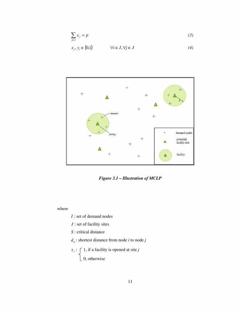
In Figure 3.1, two facilities are located and their service areas with radii of S are

indicated transparently. The demand points that are within critical distances of

facilities are covered. The points that are further are uncovered.

MCLP is modeled by Church and ReVelle (1974) as follows:

Max ∑∈Ii

ii ya (1)

s.t.

i

Nj

j yxi

≥∑∈

Ii ∈∀ (2)

11

pxJj

j =∑∈

(3)

{ }1,0, ∈ij yx JjIi ∈∀∈∀ , (4)

Figure 3.1 – Illustration of MCLP

where

I : set of demand nodes

J : set of facility sites

S : critical distance

ijd : shortest distance from node i to node j

:jx 1, if a facility is opened at site j

0, otherwise

12

iN : the set of facility sites that are eligible to cover demand point i,

{ }SdJjN iji ≤∈=

iy : 1, if demand at i is covered

0, otherwise

:ia population at demand node i

p : number of facilities to be located

Objective (1) maximizes the number of people covered within the critical

distance. Constraint set (2) allows coverage of demand point i if one or more

facilities are established within critical distance. Constraint (3) limits the number

of established facilities to p. Constraint set (4) ensures all variables to be binary.

HMCLP extends classical MCLP by differentiating levels of service demanded

and levels of service provided and also setting hierarchical relationships between

the differentiated servers. In HMCLP, more than one level of service is required,

where levels are categorized according to the complexity of service they provide.

High-level service is supplied by high-level facilities whereas low-level service is

supplied by both low-level and high-level facilities.

In Figure 3.2, demand points require both low and high-level services, and the

facilities are discriminated to meet these differentiated service requirements.

Critical distances of high-level facilities – 2S are larger than critical distances of

low-level facilities – 1S , since high level facilities has been thought to be more

capable and equipped, in literature.

Both levels of demand requirements are satisfied for the demand points inside the

larger circular areas (demand i2 for instance) whereas only the low-level deman d

requirements are satisfied for the ones inside the smaller circular areas (demand i1

13

Figure 3.2 – Illustration of HMCLP

for instance). High-level demand requirements of those demand points are

unsatisfied. Demand points that are outside of any of the circles above are

uncovered at all.

HMCLP is modeled as follows by Moore and ReVelle (1982):

Max ∑∈Jj

jj xf (5)

s.t.

0≥−+∑∑∈∈

ji

Ii

ij

Ii

iij xzbya Jj ∈∀ (6)

0≥−∑∈

ji

Ii

ij xzc Jj ∈∀ (7)

pyIi

i =∑∈

(8)

qzIi

i =∑∈

(9)

14

{ }1,0,, ∈iij zyx IiJj ∈∀∈∀ , (10)

where

I : set of potential facility sites

J : set of demand areas

1, if demand area j can be covered by level-1 service offered at a

ija : lower-level facility located at i ∈ I

0, otherwise


ijb : higher-level facility located at i ∈ I

0, otherwise


ijc : higher-level facility located at i ∈ I

0, otherwise

:jx 1, if demand area j is covered

0, otherwise

iy : 1, if a lower-level facility is located at site i ∈ I

0, otherwise

iz : 1, if a higher-level facility is located at site i ∈ I

0, otherwise

:jf population of demand area j

p : number of lower-level facilities to be located

q : number of higher-level facilities to be located

Objective function (5) maximizes the total population covered by both level-1 and

level-2 services. Constraint set (6) states that a demand area j∈J is covered by

level-1 service if there is at least either one lower-level facility or one higher-level

facility within its corresponding critical distance. Constraint set (7) states that a

demand area j∈J is covered by level-2 service if there is at least one higher-level

facility within its corresponding critical distance. Constraint (8) limits the number

15

of lower-level facilities in the solution to p; whereas constraint (9) limits the

number of higher-level facilities in the solution to q. Finally, constraint sets (10)

define 0–1 nature of the decision variables.

Demand points include demand requiring low-level service and demand-requiring

high-level service at the same time. In some cases, demand has to be covered by

low-level facility first and then covered by high-level facility. The role low-level

facility executes is called referral in literature.

Referral has first been studied in p-median problems in literature; where all

demand is assumed to have access to facilities and the total distance traveled in

order to access is the main concern. The 2-hierarchical uncapacitated p-median

formulation with referral by Narula and Ogbu (1983) is as follows:

Min ∑∑= =

++n

i

n

j

ijijijij dXXX1 1

120201 )( (11)

s.t.

∑=

=+n

j

iijij WXX1

0201 )( ni ,...,1= (12)

∑ ∑= =

=n

j

n

j

jiij XX1 1

0112 θ ni ,...,1= (13)

1

1

01j

n

i

ij MYX ≤∑=

nj ,...,1= (14)

2

1 1

1202j

n

i

n

i

ijij MYXX ≤+∑ ∑= =

nj ,...,1= (15)

∑=

=n

j

j pY1

11 (16)

∑=

=n

j

j pY1

22 (17)

121 ≤+ jj YY nj ,...,1= (18)

16

iij WX ≤≤ 010 , iij WX ≤≤ 020 , MX ij θ≤≤ 120

ni ,...,1= ; nj ,...,1= (19)

{ }1,0, 21 ∈jj YY nj ,...,1= (20)

where

1, if the demand at location i with no facility located there,

01ijX : is allocated to a level-1 facility at location j

0, otherwise

1, if the demand at location i with no facility located there,

02ijX : is allocated to a level-2 facility at location j

0, otherwise

1, if the demand at location i with level-1 facility located there,

12ijX : is referred to a level-2 facility at location j

0, otherwise

1jY : 1, if a level-1 facility is located at location j

0, otherwise

2jY : 1, if a level-2 facility is located at location j

0, otherwise

1p : number of level-1 facilities to be located

2p : number of level-2 facilities to be located

n : number of potential locations

iW : demand at location i; where ∑=

=n

i

iWM1

θ : fraction of demand referred from a level-1 facility to level-2 facility;

where 10 ≤≤ θ

ijd : minimum travel distance between locations i and j

Objective function (11) minimizes the total distance traveled for demand assigned

to level-1 facilities, demand assigned to level-2 facilities and demand referred to

17

level-2 facilities from level-1 facilities. Constraint set (12) ensures that demand at

each location is allocated to a facility. Constraint set (13) states that a fraction θ

of total demand accumulated at level-1 facilities is referred to level-2 facilities.

Constraint sets (14) and (15) ensure that allocations are made only to locations

with facilities. Constraints (16) and (17) state that 1p level-1 facilities and 2p

level-2 facilities can be opened. Constraint set (18) ensures that at most one

facility can be opened in each location.

Another critical distance 3S ; that is the maximum distance; referral of demand

from low-level facilities to high-level facilities is possible, is defined in addition

to critical distances for coverage of demand by low-level facilities 1S and

coverage of demand by high-level facilities 2S .

Thus, the low-level facilities within 3S distance to high-level facilities are said to

be covered by high-level facilities. This implies that demand points covered by

these low-level facilities are also covered by high-level facilities, although

demand points are not within 2S distance of high-level facilities.

In Figure 3.3, low-level facilities have low-level demand service area (of radii

1S ) whereas high-level facilities have both high-level demand service area (of

radii 2S ) and referral area (of radii 3

S ).

Demand points only within 1S distance of low-level facilities (demand i1 for

instance), would be uncovered by high-level facilities if there were no referral.

However, in this case, since low-level facility j1 is within 3S distance of high-

level facility j2, demand i1 is also covered. High-level demand at point i1 is

satisfied by high-level facility at j2 via referral.

18

Figure 3.3 – Illustration of MCLP with referral

Partial coverage is another relaxation to the classical MCLP that extends classical

concept of binary coverage by defining one more critical distance. Binary

coverage models assume that coverage is 100% till the critical distance and fall

crisply down to 0% after critical distance. Difference of coverages in two sides of

borders is softened by introducing the second critical distance. Henceforth, the

first critical distance is called the minimum critical distance – S and the second

critical distance is called the maximum critical distance – T.

The coverage concept, therefore, is modified and concept of quality is introduced.

Demand points that are within S distance to a facility are said to be covered,

points that are further than T distance are said to be uncovered, and the points that

are located between S-T distances are partially covered; that is the quality of

service decreases as distance to the center increases. Coverage takes continuous

values between 0 and 1 to represent quality.

19

The MCLP-P is modeled by Karasakal and Karasakal (2004) as follows:

Max ∑∑∈ ∈Ii Mj

ijij

i

xc (21)

s.t.

∑∈

=Jj

j Py (22)

jij yx ≤ iMjIi ∈∈∀ , (23)

∑∈

≤iMj

ijx 1 Ii ∈∀ (24)

}1,0{∈jy Jj ∈∀ (25)

}1,0{∈ijx iMjIi ∈∈∀ , (26)

where

I : index set of demand points,

J : index set of potential facility sites,

P: number of facilities to be sited,

iM : set of facility sites that can either fully or partially cover the demand

point i,

S: the maximum full coverage distance,

T: the maximum partisl coverage distance, ( ST > ),

ijD : the travel distance between the facility j and demand point i,

ijC : the level of coverage provided by the facility j to the demand point i,

1, if SDij ≤

ijC : ),( ijDf if ,TDS ij ≤< )1)(0( << ijDf

0, otherwise

:jy 1, if a facility is sited at j,

0, otherwise

1, if the demand at point i is either partially or fully covered by a

ijx : facility at j,

0, otherwise

20

Objective function (21) maximizes the coverage level within the maximum

critical distance T. Constraint (22) limits the number of facilities to be sited to P.

Constraint set (23) ensures that if a facility is not sited at j, then demand at i can

not be covered by j. Constraint set (24) ensures that all demand points can be

covered by at most one facility. If there are more than one facilities covering a

demand point, the facility that provides the maximum coverage will be selected

which is forced by the objective function. Constraint sets (25) and (26) impose

binary restriction on the decision variables.

Figure 3.4 – Illustration of partial coverage

In Figure 3.4, the demand points within circular area framed by continuous lines

(demand point i1 for instance) are 100% covered whereas the points inside dashed

lines but outside the continuous lines (demand point i2 for instance) are partially

covered. Coverage is inversely proportional with the distance between the

21

demand and the facility nodes. Points outside all of the circular areas are totally

uncovered.

The revealed model, thus, can be represented as in Figure 3.5.

Figure 3.5 – Illustration of HMCLP with referral in the presence of

partial coverage

In the above figure, all demand points require both low and high-level service.

The potential facility sites are appropriate for establishment of both types of

facilities. Frames of binary coverage and partial coverage are indicated with

continuous and dashed lines, sequentially.

Demand i2 is covered by high-level facility j2 and low level facility j1; therefore

both low and high-level service requirements are satisfied. High-level service

22

requirement is either directly partially satisfied by high-level facility j2 or it is

indirectly satisfied by high-level facility j2 via referral from low-level facility j1.

Demand i1 is covered by low-level facility j1. Although it is not covered by any

high-level facility, both low and high-level service requirements of it is also

satisfied, since low-level facility j1 is covered by high-level facility j2.

3.2 MOTIVATION

Consider a health service system. If you have a complaint of sore throat, you go

to a health center, since you know that this level of service is provided by a health

center. If you have a heart attack, you are directly taken to a hospital, since it is

known that heart attack is emergency situation and a health center is not equipped

enough to manage necessary operations for a heart attack.

However, if you have a headache; the reason may be that you are too tired and

you need just vitamins, but on the other hand it may be that you have a serious

tumor in the membrane of your brain and you should have a very critical surgery

that carries 80% risk of death. In such a situation, you need a preliminary

evaluation. If the reason of the headache is tiredness, then you should remain in

the health center, but if the reason is a tumor, then you should be referred to a

hospital.

Another example may be from the battlefield. Suppose that we have a battery-

headquarters that commands 3 batteries. If target is considered to be within the

capacity of the batteries by the forward observer then the target is handled by the

battery headquarter. If the target can not be destroyed by the batteries, it is

handled by the upper-headquarters and determined to be destroyed by rocket

missiles.

23

However, if the target can not be evaluated by the forward observer, then it

should be evaluated in the battery-headquarters. After evaluation, if decision is

finalized as batteries destroy the target then operation stays in the battery-

headquarters. If battery-headquarters decide that batteries are not capable, then

the decision of with which weapon to destroy should be referred to the upper-

headquarters.

In these two cases, the question of “If the upper level service provider gives both

types of services, then why do not we directly assign demand to the upper level

instead of creating another level?” may arise. The reason is assigning whole

demand directly to the hospital or all targets directly to the upper-headquarters is

costly since giving a low-level service by a high-level server is costly and

undesirable. Carrying out the procedure in such a way is less complicated and

more efficient.

So referral in a hierarchical service system which includes both referral from low-

level to high-level server and direct assignment to high-level server is motivated

by the third type of demand that has preliminary evaluation about its

characteristic. In addition to referral, we need to explain the motivation under the

partial coverage.

Partial coverage is directly related to the quality of service, but it should not be

thought as probability. Consider a hospital that provides ambulances in case of

emergency. Say that, the critical time for access of ambulance to the demand

point is determined as 3 minutes. If an ambulance can reach the point within 3

minutes, then it can prevent death of a person having a heart attack, but if the

demand point is further than 3 minutes, the person can not have emergency

service from this hospital.

Suppose there is another person within 4 minutes of this hospital. If he has a heart

attack and he expects service from this hospital, then he would not take it.

24

However, what if this person has gastric bleeding? Then it may be acceptable to

serve this person within 4 minutes. It is true that, the hospital can not prevent his

heart attack, but it can prevent his gastric bleeding. If he is further, say within 5

minutes range of the hospital, the hospital can not prevent this person’s gastric

bleeding in this case, but only his appendicitis.

If we look at the problem from a different angle, consider a person having

gastritis within 5 km of a hospital. If he had a heart-related problem or he had to

have a surgery, he would tolerate making 5 km way to hospital. However, for

gastridis he would tolerate at most 4 km but not 5 km and may give up the idea of

visiting hospital.

Drezner, Wesolowsky and Drezner (2004) describe very interesting applications

of partial coverage concept. They consider a public facility such as a post office

for objective of customer satisfaction. If people are within l distance, they are

very satisfied with the service, that they only walk to the facility. People who live

within a distance of between l and u have a linearly decreasing satisfaction, that

they drive to the facility. People who live beyond a distance u are very

dissatisfied because they may not even use the facility at all. Maximizing the

satisfaction is in fact what MCLP-P formulation is.

They consider another scenario which is valid in medical facilities. They interpret

partial coverage as the rate of survival for the heart attack victims. Up to a

determined time (distance l), survival rate is 100%. Then survival rate decreases

with the time taken to reach the patient, and after a certain time (distance u)

survival rate reaches a constant value because the patient either did not survive by

that time or his condition is stabilized and he will survive even with very late

help.

They explained other scenarios such as delivery problem, competitive location,

dense competition and radio/TV/cellular transmitter.

25

Applications are also found in military. Suppose there is an observer airplane that

observes ships. Up to 5 miles, the plane can observe ships of 20 m long; but in 6

miles, the precision of sight deteriorates and it observes ships if they are at least

30 m long.

In all the applications, there is a decrease in quality. Within the maximum critical

distance (u or T) the facilities can not be regarded as supplying the same service

that they supply within the minimum critical distance (l or S), but they can not

also be regarded as supplying no service. There is sacrifice from quality (such as

not being able to prevent death of person having heart attack 4 minutes away the

hospital, not being able to see 20 m long ships within 6 miles distance), but also

an advantage (such as not being obliged to establish another hospital to prevent

gastric bleeding of the person in 4 minutes, not being obliged to charge another

observing plane to detect 30 m long ships).

3.3 PROBLEM DEFINITION

Given a set of demand points and a set of potential facility sites, the objective is

to maximize the total amount of demand covered with a pre-determined number

of successively inclusive hierarchical facilities; where coverage is defined as

being within a pre-determined critical distance. This general concept of

hierarchical facilities is reduced to health centers and hospitals in our problem.

Demand has both low-level and high-level requirements that have to be satisfied.

In addition to this, it may have a characteristic that can not be categorized in

advance. Thus, people of the same demand point may need low-level service

only, high-level service only or both levels of services at the same time; where

demand point is regarded uncovered unless all levels of service requirements are

26

satisfied. However, demand at a demand point can not be fractioned; that is

demand can not be allocated to different facilities.

High-level service can only be provided by hospitals whereas low-level service

can be provided by both health centers and hospitals, since hierarchy is

successively inclusive. This hierarchic structure obliges demand to be covered by

hospital directly or indirectly or not to be covered at all; that is either demand is

covered by a hospital that is supplying both low and high-level services or it is

referred to a hospital via a health center covering it or it is not covered at all. All

service requirements of a covered demand point are satisfied; that is there exists

no demand point covered only by health centers. Referral here represents

coverage of demand by a health center that is covered by a hospital. This enables

whole low-level and high-level demand to be satisfied. Low-level demand is

satisfied by health center or hospital directly. High-level demand, on the other

hand, is satisfied by hospital directly or by referral indirectly.

Figure 3.6 – Illustration of the problem

27

In Figure 3.6, low-level demand at node i1 is fully covered by health center at

node j1. Low-level demand at node i2 can either be fully covered by health center

at node j1 or be partially covered by hospital at node j2. High-level demand at

node i2 is partially covered by hospital at node j2. High-level demand at node i1 is

non-covered unless demand is referred. In the above graph, since demand at node

i1 is covered by health center at node j1 and health center at node j1 is also covered

by hospital at node j2; high-level demand at node i1 is said to be covered via

referral.

In addition to the classical coverage concept, coverage here is modeled with a

decreasing function rather than binary, by defining minimum and maximum

critical distances. Coverage is considered as full-coverage before minimum

critical distance S and as non-coverage after maximum critical distance T. In

between, it is considered as a linearly decreasing function that is inversely

proportional with distance; representing partial coverage or in other words, the

quality of coverage.

In Figure 3.7, coverage is 1 until minimum critical distance, linearly converges to

0 from minimum critical distance to maximum critical distance, and is 0 after

maximum critical distance.

In classical HMCLP models, weight of demand at a demand point is separated

into 1id - demand requiring low level service and 2

id - demand requiring high

level service; provided that 1id + 2

id = id where id is the total weight. Coverage is

used to be calculated using these weights. However; in our model, demand is not

needed to be separated.

28

Figure 3.7– Coverage vs. distance function

In classical hierarchical approach, a demand point is either covered by low-level

facility only or high-level facility only or covered by both or not covered at all. In

the case that demand point is covered only by a low-level facility, the portion of

demand that requires high-level service stays unsatisfied. To subtract this portion

from coverage calculations, it is needed to discriminate weights of demands.

Thus, each demand type should contribute separately to coverage calculations.

In our case, however; such a situation is never encountered; that is in any demand

point it is impossible to satisfy demand requiring low-level service but unsatisfy

demand requiring high-level service; because of our obligatory hierarchic

assignment using referral. In our model, since every demand point has either to be

covered by hospital (directly or via referral) or not to be covered at all; it is not

needed to consider low-level demand weights, thus to discriminate weights of

demands.

29

3.4 ASSUMPTIONS

1. Given a set of nodes and a set of edges that combine these nodes; demand

points are assumed to be accumulated only at nodes.

2. Given a set of nodes and a set of edges, facilities are assumed to be

established only at nodes.

3. The decrease in the quality of coverage between critical distances S and T

is assumed to follow a linear pattern.

4. A health center can be opened only if it can be referable to a hospital. If a

health center is not within referable critical distance of hospitals, it is not

allowed to be opened.

5. Demand can not be split at assignment; it is assigned to at most one

facility. If it is assigned to a health center, a pre-determined percent δ of

it is referred to the corresponding hospital that is matched with the health

center. In experimentation, it is assumed that 1=δ , all demand assigned

to health centers is referred to hospitals.

6. At a demand point, demand requiring low-level service and demand

requiring high-level service are not differentiated. The total demand is

designated by id . Each demand point requires both high-level and low-

level services.

7. There is no differentiation considered in critical distances of high-level

facility providing high-level service and low-level service, as in some

studies in literature. We assume that both high- and low-level

requirements are satisfied when demand is covered by high-level facilities.

It is identical to utilization of minimum of critical distances of high-level

30

facility providing low-level service and high-level facility providing high-

level service for both coverages.

8. There exists no restriction about opening health centers and hospitals in

the same place.

3.5 MATHEMATICAL FORMULATION

3.5.1 MODEL

Max ∑∑ ∑∑ ∑∑∑∈ ∈ ∈ ∈ ∈∈ ∈

++

Ii Jj Jj Jk

jkjk

Ii

ijijiijijiijij

Ii Jj

i ycxcdwxcdwxcdw311

322

211

1 δ

(27)

s.t.

∑∈

=Ji

i qz (28)

∑∑∈∈

≤Jj

ij

Ii

py (29)

∑∈

≤Jk

jkijij yax11 JjIi ∈∈∀ , (30)

jijij zax 22 ≤ JjIi ∈∈∀ , (31)

1)( 21 ≤+∑∈Jj

ijij xx Ii ∈∀ (32)

jijij zay 3≤ JjJi ∈∈∀ , (33)

1≤∑∈Jj

ijy Ji ∈∀ (34)

{ }1,01 ∈ijx JjIi ∈∈∀ , (35)

{ }1,02 ∈ijx JjIi ∈∈∀ , (36)

{ }1,0∈ijy JjJi ∈∈∀ , (37)

{ }1,0∈iz Ji ∈∀ (38)

31

where

I: set of demand points

J: set of potential facility sites to open health center and/or hospital,

J ⊂ I

id : demand at i (weight of node i )

1, if demand at node i is within 1T distance of health center at

1ija : node j

0, otherwise

1, if demand at node i is within 2T distance of hospital at node

2ija : j

0, otherwise

1, if health center at node i is within 3T distance of hospital at

3ija : node j

0, otherwise

1, if demand at node i is within 1S distance of health center at

node j

1ijc : ( 1T – ijdist ) / ( 1T – 1

S ), if demand at node i is between 1S

and 1T distance of health center at node j

0, otherwise

1, if demand at node i is within 2S distance of hospital at node

j

2ijc : ( 2T – ijdist ) / ( 2T – 2

S ), if critical demand at node i is

between 2S and 2T distance of hospital at node j

0, otherwise

32

1, if health center at node i is within 3S distance of hospital at

node j

3ijc : ( 3T – ijdist ) / ( 3T – 3

S ), if health center at node i is between

3S and 3T distance of hospital at node j

0, otherwise

ijdist : distance between nodes i and j

1S

: minimum critical distance for demand-by-health center coverage

2S

: minimum critical distance for demand-by-hospital coverage

3S

: minimum critical distance for health center-by-hospital coverage

1T : maximum critical distance for demand-by-health center coverage

2T : maximum critical distance for demand-by-hospital coverage

3T : maximum critical distance for health center-by-hospital coverage

1ijx : 1, if demand at node i is covered by a health center at node j

0, otherwise

2ijx : 1, if demand at node i is covered by a hospital at node j

0, otherwise

1, if health center at node i is opened and covered by a

ijy : hospital at node j

0, otherwise

iz : 1, if hospital is opened at node i

0, otherwise

1w : weight of first term of objective function, importance deemed to

coverage of demand by health centers

2w : weight of second term of objective function, importance deemed to

coverage of demand by hospitals

33

3w : weight of third term of objective function, importance deemed to

referral of demand to hospitals via health centers

δ : fraction of demand that has to be referred to hospitals via health

centers

Objective (27) maximizes the total demand covered; total of weighted coverage

provided by health centers to demand points, weighted coverage provided by

hospitals to demand points and weighted coverage provided by hospitals to

demand referred via health centers. Note that the objective function is nonlinear.

Constraint set (28) fixes the number of hospitals to be opened at q. Constraint set

(29) limits the number of referrals -assignments from health centers to hospitals-

with p. This constraint set in fact, limits the number of opened and covered health

centers, together with constraint set (34). Referral is required to be considered in

order to limit the number, because if a health center is not able to refer its demand

it is not allowed to be opened. The constraint should be less than or equal to,

otherwise infeasibility may occur depending on the problem instance.

Constraint set (30) ensures that demand at node i can be covered by a health

center at node j only if demand at node i is within 1T critical distance of health

center at node j and health center at node j is assigned to a hospital. Constraint set

(31) ensures that demand at node i can be covered by a hospital at node j only if

demand at node i is within 2T critical distance of an opened hospital at node j.

Constraint set (32) restricts demand at node i to be covered by only one facility or

not covered at all.

Constraint set (33) ensures that health center at node i can be covered by a

hospital at node j only if health center at node i is within 3T critical distance of

an opened hospital at node j. Constraint set (34) restricts health center at node i to

be covered by at most one hospital. Coverage in this relationship can also be

considered as assignment or matching as well.

34

Constraint sets (35)-(38) ensure all variables to be binary.

Complexity of the model is O( |||| JI )., since

# of variables: ||||||*||*2 2 JJJI ++ = )1||||2*(|| ++ JIJ : O( |||| JI ) and

# of constraints: ||||||||*||*2 2 JJIJI +++ : O( |||| JI ).

The model also includes a quadratic element in the third term of the objective

function which is needed to be removed. The linearization is carried out in two

different ways.

3.5.2 LINEARIZED MODELS

3.5.2.1 LINEARIZED MODEL 1

Objective function is changed as follows

Max ∑∑ ∑∑∑∑∑∈ ∈ ∈ ∈ ∈∈ ∈

++i Jj Jj Jk

ijkjk

Ii

ijiijijiijij

Ii Jj

i uccdwxcdwxcdw31

322

211

1 δ (27a)

and the following constraints are added,

( )jkijijk yxu +≤ 1

2

1 JkJjIi ∈∈∈∀ ,, (39)

{ }1,0∈ijku JkJjIi ∈∈∈∀ ,, (40)

where

1, if demand at node i is referred to hospital at node k via

ijku : health center at node j

0, otherwise

35

Objective function (27a) is the linearized form of objective function (27) by

introduction of decision variable ijku . Constraint set (39) ensures that referral

from demand point i to hospital k via health center j is possible only when

demand point i is covered by health center j (i.e. 1=ijx ) and health center j is

covered by hospital k (i.e. 1=jky ). Constraint set (40) ensures that ijku are binary.

Complexity of the model is increased to O( 2|||| JI ), since

# of variables: 22 ||*||||||||*||*2 JIJJJI +++ =

|)|||1||||2*(|| JIJIJ +++ : O( 2|||| JI ) and

# of constraints: 22 ||*||||||||||*||*2 JIJJIJI ++++ : O( 2|||| JI ).

3.5.2.2 LINEARIZED MODEL 2

Objective function is changed as follows

Max ∑∑ ∑∑∑∑∈ ∈ ∈ ∈∈ ∈

++Ii Jj Jj Jk

jkijijiijij

Ii Jj

i uwxcdwxcdw 322

211

1 (27b)

and the following constraints are added,

31jk

Ii

ijijijk cxcdu

≤ ∑

∈

δ JkJj ∈∈∀ , (41)

jkjk Myu ≤ JkJj ∈∈∀ , (42)

{ }1,0∈jku JkJj ∈∈∀ , (43)

where

jku : total weight accumulated in health center at node j to be referred to

hospital at node k

M : a large number

36

Objective function (27b) is the linearized form of objective function (27) by the

introduction of decision variable jku . Constraint set (41) limits the weight

referred from health center j to hospital k by coverage weighted total demand

accumulated in health center j, that is the total weight of demand point i’s covered

by health center j. Constraint set (42) sets the weighted coverage at node j to zero

if no coverage is provided from node k. In case of coverage, the constraint set

does not put bounds on the amount. Constraint set (43) ensures that jku are

binary.

Complexity of the model is stayed at O( |||| JI ) in this linearization, since

# of variables: 22 ||||||||*||*2 JJJJI +++ = |)|1||||2*(|| JJIJ +++ :

O( |||| JI ) and

# of constraints: 22 ||||||||||*||*2 JJJIJI ++++ : O( |||| JI ).

The problem is NP-hard; that is complexity increases exponentially with problem

size. In most of the uncapacitated covering problems assignment is not needed.

The information of whether a demand point is covered or not is sufficient, it is not

required to keep which facility covers which demand point. However,

introduction of partial coverage requires assignment, since coverage is calculated

using distances between demand and facility nodes.

The following sets are defined in order to reduce problem size.

{ }111 =∧∈∧∈∋= ijij aJjIiijM : set of demand point-health center

pairs that are in 1T distance to each

other

{ }122 =∧∈∧∈∋= ijij aJjIiijM : set of demand point-hospital pairs

that are in 2T distance to each other

37

{ }133 =∧∈∧∈∋= ijij aJjJiijM : set of health center-hospital pairs

that are in 3T distance to each other

3.5.3 LINEARIZED REDUCED MODELS

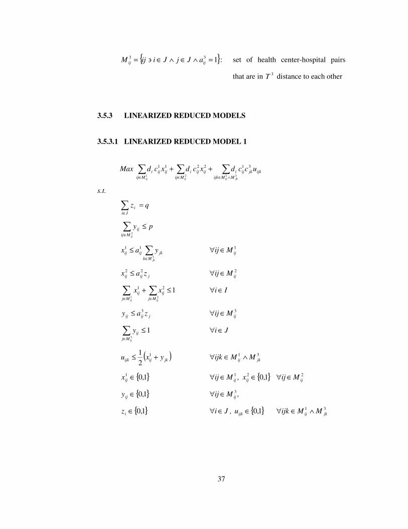
3.5.3.1 LINEARIZED REDUCED MODEL 1

Max ∑∑∑∧∈∈∈

++3121

312211

jkijijij MMijk

ijkjkiji

Mij

ijijiijij

Mij

i uccdxcdxcd

s.t.

∑∈

=Ji

i qz

∑∈

≤3ijMij

ij py

∑∈

≤3

11

jkMk

jkijij yax 1ijMij ∈∀

jijij zax 22 ≤ 2ijMij ∈∀

11 2

21 ≤+∑ ∑∈ ∈ij ijMj Mj

ijij xx Ii ∈∀

jijij zay 3≤ 3ijMij ∈∀

13

≤∑∈ ijMj

ijy Ji ∈∀

( )jkijijk yxu +≤ 1

2

1

31jkij MMijk ∧∈∀

{ }1,01 ∈ijx 1ijMij ∈∀ , { }1,02 ∈ijx

2ijMij ∈∀

{ }1,0∈ijy 3ijMij ∈∀ ,

{ }1,0∈iz Ji ∈∀ , { }1,0∈ijku 31jkij MMijk ∧∈∀

38

3.5.3.2 LINEARIZED REDUCED MODEL 2

Max ∑∑∑∈∈∈

++321

2211

jkijij Mjk

jk

Mij

ijiji

Mij

ijiji uxcdxcd

s.t.

∑∈

=Ji

i qz

∑∈

≤3ijMij

ij py

∑∈

≤3

11

jkMk

jkijij yax 1ijMij ∈∀

jijij zax22 ≤

2ijMij ∈∀

11 2

21 ≤+∑ ∑∈ ∈ij ijMj Mj

ijij xx Ii ∈∀

jijij zay3≤

3ijMij ∈∀

13

≤∑∈ ijMj

ijy Ji ∈∀

31

1jk

Mi

ijijijk cxcdu

ij

≤ ∑

∈

3jkMjk ∈∀

jkjk Myu ≤ 3jkMjk ∈∀

{ }1,01 ∈ijx 1ijMij ∈∀ , { }1,02 ∈ijx

2ijMij ∈∀

{ }1,0∈ijy 3ijMij ∈∀ ,

{ }1,0∈iz Ji ∈∀ , { }1,0∈jku 3jkMjk ∈∀

3.6 AN EXAMPLE AND SENSITIVITY ANALYSIS

The formulation developed for HMCLP(R)-P is illustrated on a 50-node example

problem. Suppose the budget gives opportunity to establish 14 health centers and

6 hospitals.

39

The parameters are set at S1 = 30, S2 = 60, S3 = 80, T1 = 50, T2 = 80, T3 = 100 and

w1 = 1, w2 = 1, w3 = 1, δ = 1 initially. The optimal configuration is presented in

Figure 3.8.

Problem

Parameters

Assignment of Demand to

Health Centers (Demand-

Health Center)

Assignment of Demand to Hospitals (Demand-Hospital)

Refer of Health Centers to Hospitals (Health Center-

Hospital)

Opened Hospitals

Optimal Result

Total People

Covered

original problem

S1 = 30 S2 = 60 S3 = 80 T1 = 50 T2 = 80

T3 = 100 w1 = 1 w2 = 1 w3 = 1

δ = 1

1-1

9-9

10-10

12-12

14-21

15-1

16-16

17-17

18-18

19-19

21-21

25-19

26-16

27-27

30-30

32-32

36-38

37-30

38-38

41-38

50-50

5-5

13-13

23-31

31-31

45-32

1-1

9-13

10-5

12-31

16-31

17-31

18-13

19-25

21-25

27-5

30-5

32-32

38-32

50-25

1

5

13

25

31

32

611.71 346

Figure 3.8 – Optimal configurations of facilities for the original problem

40

The setting for critical distances may be narrower or larger as presented in figure

3.9.

Problem Parameters

Assignment of Demand to Health

Centers (Demand-Health

Center)


Refer of Health

Centers to Hospitals (Health Center-

Hospital)

Opened Hospitals

Optimal Result

Total People

Covered

1

S1 = 50 S2 = 80 S3 = 80 T1 = 60

T2 = 120 T3 = 120 w1 = 1 w2 = 1 w3 = 1

δ = 1

1-1

5-37

9-9

10-10

12-16

14-21

15-1

16-16

17-17

19-25

21-21

25-25

26-16

27-27

29-50

30-37

31-16

32-38

35-35

36-38

37-37

38-38

39-39

41-38

45-45

49-39

50-50

6-5

8-25

13-9

23-31

34-25

40-36

1-1

9-9

10-5

16-31

17-31

21-25

25-25

27-5

35-9

37-5

38-36

39-36

45-36

50-25

1

5

9

25

31

36

703,20 401

Figure 3.9 – Changes in optimal configurations of facilities with changes

in all critical distances

41

Problem

Parameters



Center)


Refer of Health


Hospital)

Opened Hospitals

Optimal Result

Total People

Covered

2

S1 = 20 S2 = 60 S3 = 60 T1 = 30 T2 = 90 T3 = 90 w1 = 1 w2 = 1 w3 = 1

δ = 1

5-5

9-9

10-10

12-12

15-15

16-16

17-17

19-25

21-21

25-25

27-27

30-37

32-32

37-37

38-38

41-38

45-45

1-1

2-32

6-5

13-9

14-32

23-31

26-31

31-31

36-32

5-5

9-9

10-5

12-31

15-1

16-31

17-31

21-19

25-19

27-5

32-32

37-5

38-32

45-32

1

5

9

19

31

32

551.28 328

Figure 3.9 (continued) – Changes in optimal configurations of facilities

with changes in all critical distances

Figure 3.9 indicates that even small adjustments in parameter settings may alter

the settlement of the facilities. Therefore, the characteristics of the region, the

42

health culture and the experimented quality that can be supplied should be treated

as important factors in determination of the parameters.

In Figure 3.8, there is another issue that we need to discuss. Although it is not

restricted by the formulation to establish a health center and a hospital at the same

site, in the optimal solution it is not expected to have such a case since

establishing both facilities in the same site is inefficient. If there is an extra

facility, it should be established in a different site to cover additional demand.

However, in the above configuration, both a health center and a hospital are

placed in node 32.

The importance of setting parameters comes into scene at this point. Although the

model explained in Section 3.5 is verified; without correct setting of parameters it

does not reflect entire requirements. The expectation is having a configuration as

dispersed as possible. Then the reason behind locating both facilities at the same

site should be analyzed.

The constraint of “health centers can be opened only if they can be referred to

hospitals” causes hospitals in the middle with batches of health centers around

them, which are within the referral critical distances of the hospitals. This

accumulation can be prevented by enlarging the referral critical distances.

However, that technical requirement coincides with real life. Hospitals frequently

serve people coming from distant places because of their special capabilities or

abilities of their doctors. Thus, having coverage for distant places even if

coverage level is low sounds reasonable.

43

Problem

Parameters



Center)


Refer of Health


Hospital)

Opened Hospitals

Optimal Result

Total People

Covered

3

S1 = 50 S2 = 80 S3 = 80 T1 = 60

T2 = 120 T3 =

}{max ijij dist

w1 = 1 w2 = 1 w3 = 1

δ = 1

1-1

3-3

5-5

9-9

12-16

14-21

15-1

16-16

18-18

19-25

21-21

25-25

16-16

27-27

28-28

30-30

33-33

35-35

37-30

39-39

49-39

4-7

6-6

7-7

10-6

17-23

23-23

29-29

31-23

32-32

34-40

36-32

38-32

40-40

41-40

42-29

45-32

46-7

50-29

1-6

3-6

5-6

9-6

16-23

18-6

21-32

25-29

27-6

28-29

30-6

33-7

35-6

39-40

6

7

23

29

32

40

726.83 479


in referral critical distances

44

Changed Problem

Parameters



Center)


Hospitals (Demand-Hospital)

Refer of Health


Hospital)

Opened Hospitals

Optimal Result

Total People

Covered

4

S1 = 30 S2 = 60

S3=0 T1 = 50 T2 = 80

T3

= }{max ijij dist

w1 = 1 w2 = 1 w3 = 1

δ = 1

1-1

3-3

5-5

9-9

12-16

14-21

15-1

16-16

18-18

19-25

21-21

25-25

26-16

27-27

28-28

30-30

33-33

35-35

37-30

39-39

49-39

4-7

6-6

7-7

10-6

17-23

23-23

29-29

31-23

32-32

34-40

36-32

38-32

40-40

41-40

42-29

45-32

46-7

50-29

1-6

3-6

5-6

9-6

16-23

18-6

21-32

25-29

27-6

28-29

30-6

33-7

35-6

39-40

6

7

23

29

32

40

706.48 479


with changes in referral critical distances

In Figure 3.10, the referral critical distances are adjusted. Enlargement of

maximum critical distance for referral provides the desired effect of homogeneous

dispersal of health centers and hospitals. Since any health center in any district

45

can be referred to any hospital, establishing health centers and hospitals in

different places earns meaning.

The configurations are consistent with the ‘Total People Covered’ values

presented in last columns. It calculates the total coverage without the

consideration of partial coverage; that is the total weight within colored coverage

areas. This eliminates the consideration of quality but dwells on quantity.

Increasing the maximum critical distance of referral to infinity -which is identical

to the maximum distance between any nodes-, yields maximum amount of net

coverage.

The fraction of people referred from health centers to hospitals (δ ) is another

important parameter. If the referral rate is small, the amount directly assigned to

hospitals increases. This is same with having the weight of the third term of the

objective function (w3) as 0.1.

46

Problem

Parameters


Health Centers (Demand-Health

Center)


Refer of Health


Hospital)

Opened Hospitals

Optimal Result

Total People

Covered

5

S1 = 30 S2 = 60 S3 = 80 T1 = 50 T2 = 80

T3 = 100 w1 = 1 w2 = 1 w3 = 1

δ = 0.1

1-15

6-6

9-9

10-10

12-12

15-15

16-16

17-17

18-18

19-25

21-21

25-25

26-16

27-27

40-40

42-42

45-45

5-5

13-13

14-38

23-31

29-29

30-5

31-31

32-38

36-38

37-5

38-38

41-38

50-29

6-5

9-13

10-5

12-31

15-1

16-31

17-31

18-13

21-38

25-29

27-5

40-38

42-29

45-38

1

5

13

29

31

38

392.72 374


in referred fraction

47

Problem

Parameters



Center)


Refer of Health


Hospital)

Opened Hospitals

Optimal Result

Total People

Covered

6

S1 = 30 S2 = 60 S3 = 80 T1 = 50 T2 = 80

T3 = }{max ijij dist

w1 = 1 w2 = 1 w3 = 1

δ = 0.1

1-1

3-3

15-1

18-18

19-19

25-19

27-27

28-28

30-30

33-33

34-34

35-35

37-30

39-49

40-40

45-45

49-49

50-50

4-7

5-10

6-10

7-7

9-9

10-10

12-16

13-9

14-14

16-16

17-23

21-14

23-23

26-26

31-23

32-14

38-14

41-14

46-7

1-10

3-10

18-10

19-14

27-10

28-10

30-10

33-7

34-14

35-9

40-14

45-14

49-16

50-10

7

9

10

14

16

23

496.11 479


with changes in referred fraction

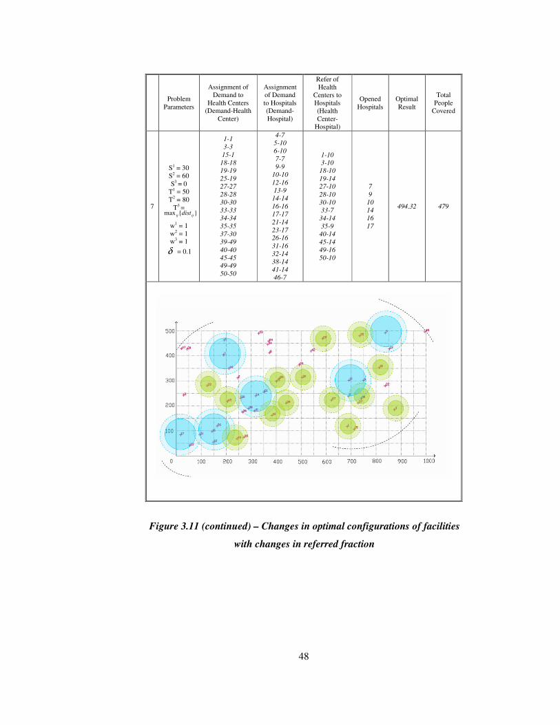
48

Problem

Parameters



Center)


Refer of Health


Hospital)

Opened Hospitals

Optimal Result

Total People

Covered

7

S1 = 30 S2 = 60 S3 = 0

T1 = 50 T2 = 80

T3 = }{max ijij dist

w1 = 1 w2 = 1 w3 = 1

δ = 0.1

1-1

3-3

15-1

18-18

19-19

25-19

27-27

28-28

30-30

33-33

34-34

35-35

37-30

39-49

40-40

45-45

49-49

50-50

4-7

5-10

6-10

7-7

9-9

10-10

12-16

13-9

14-14

16-16

17-17

21-14

23-17

26-16

31-16

32-14

38-14

41-14

46-7

1-10

3-10

18-10

19-14

27-10

28-10

30-10

33-7

34-14

35-9

40-14

45-14

49-16

50-10

7

9

10

14

16

17

494.32 479



49

Problem

Parameters



Center)


Refer of Health


Hospital)

Opened Hospitals

Optimal Result

Total People

Covered

8

S1 = 30 S2 = 60 S3 = 50 T1 = 50 T2 = 80

T3 = 300 w1 = 1 w2 = 1 w3 = 1

δ = 0.1

1-1

3-3

15-1

17-17

18-18

19-25

25-25

27-27

28-28

30-30

33-33

34-34

35-35

37-30

39-49

40-40

45-45

49-49

4-7

5-10

6-10

7-7

9-9

10-10

12-16

13-9

14-14

16-16

21-14

26-16

29-29

31-16

32-14

38-14

41-14

42-29

46-7

50-29

1-10

3-10

17-16

18-10

25-29

27-10

28-29

30-10

33-7

34-14

35-9

40-14

45-14

49-16

7

9

10

14

16

29

489.10 482



50

The referral rate affects the configuration. When referral rate is large, demand is

forced to be assigned to health centers first and then to be referred to hospitals. In

this way, it is counted by both the first and the third terms of the objective

function. Figure 3.11 demonstrates that the largest effect is obtained with the

referral critical distances of 50 and 300. Consistently, the value of ‘Total People

Covered’ is the highest amongst all.

Determination of objective function is another critical factor for application of the

model. The current objective function reflects desire of achievement of three

objectives

– low-level coverage of demand nodes by health centers,

– high-level coverage of demand nodes via referral that are already

covered by health centers, and

– low and high-level coverage of demand nodes by hospitals

with equal importance, since these objectives are combined with weights of 1 (w1

= w2 = w

3 = 1). However, the preference for different objectives may be different.

Figure 3.11 also demonstrates the situation of weight of the third term of the

objective function (w3) being 0.1 whereas rate of referral (δ ) is 1.

Another modification that equalizes the importance of direct coverage by hospital

and coverage via referral is changing the weight of coverage of low-level demand

by health centers (w1) to 0. The intuition behind this modification is that, there is

a double coverage counting for the demand points that are firstly covered by

health centers and then referred to hospitals, when δ = 1. The low-level coverage

and high-level coverage contribute to objective function separately with equal

importance. However, since there is no possibility that low-level demand of a

demand point is remained unsatisfied while high-level demand of that demand

point is satisfied; satisfaction of high-level demand via referral guarantees

satisfaction of low-level demand by health centers. Since the desire is to cover all

levels of as much as possible demand, and covering high-level ensures covering

51

all levels; the objective function can be re-defined as combination of coverage of

high-level demand by hospitals and coverage of high-level demand via referral.

Figure 3.12 demonstrates the effect of change in w1.

Problem

Parameters

Assignment of Demand to Health Centers

(Demand-Health Center)


Refer of Health


Hospital)

Opened Hospitals

Optimal Result

Total People

Covered

9

S1 = 30 S2 = 60 S3 = 50 T1 = 50 T2 = 80

T3 = 300 w1 = 0 w2 = 1 w3 = 1

δ = 1

1-1

3-3

6-6

15-1

17-17

18-18

19-25

25-25

27-27

28-28

33-33

34-34

35-35

39-49

40-40

45-45

49-49

4-7

5-5

7-7

9-9

10-5

12-16

13-9

14-14

16-16

21-14

26-16

29-29

30-5

31-16

32-14

37-5

38-14

41-14

42-29

46-7

50-29

1-5

3-5

6-5

17-16

18-9

25-29

27-5

28-29

33-7

34-14

35-9

40-14

45-14

49-16

5

7

9

14

16

29

407.60 482

Figure 3.12 – Change in optimal configuration of facilities with changes

in weight of first term in objective function

52

The configuration does not differ substantially from the trial of same critical

distances with referral rate or third term weight of 0.1. The value of ‘Total People

Covered’ is the same. These two configurations are alternative solutions in fact.

The reason of improvement in dispersal when one of weights of first and third

terms are changed is that in the objective function even though it is guaranteed

that if a demand point is assigned to a health center, it is certainly referred to a

hospital and the vice versa that if a demand point is referred to a hospital then it

certainly is covered by a health center; appearance of both of these terms in the

objective function makes covering demand by health centers and referring them

two times more important than covering demand by hospitals. So, in the optimal

configuration, hospitals are found out to be located closer to the health centers in

order to achieve the two times more important covering rather than being located

in different zones.

Increasing the objective function weight of coverage of demand by hospitals to 2

reveals exactly the same configuration with decreasing the objective function

weight of coverage of demand by health centers to 0, as demonstrated in Figure

3.13.

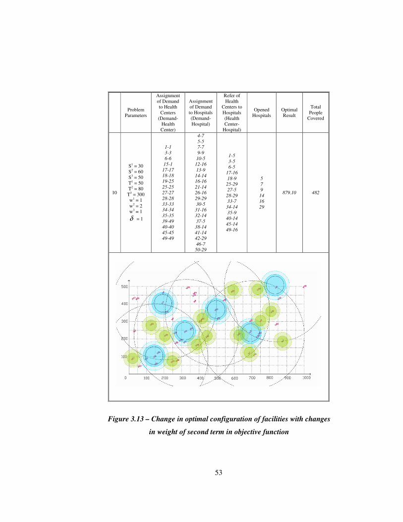
53

Problem

Parameters

Assignment of Demand to Health Centers

(Demand-Health Center)


Refer of Health


Hospital)

Opened Hospitals

Optimal Result

Total People

Covered

10

S1 = 30 S2 = 60 S3 = 50 T1 = 50 T2 = 80

T3 = 300 w1 = 1 w2 = 2 w3 = 1

δ = 1

1-1

3-3

6-6

15-1

17-17

18-18

19-25

25-25

27-27

28-28

33-33

34-34

35-35

39-49

40-40

45-45

49-49

4-7

5-5

7-7

9-9

10-5

12-16

13-9

14-14

16-16

21-14

26-16

29-29

30-5

31-16

32-14

37-5

38-14

41-14

42-29

46-7

50-29

1-5

3-5

6-5

17-16

18-9

25-29

27-5

28-29

33-7

34-14

35-9

40-14

45-14

49-16

5

7

9

14

16

29

879.10 482

Figure 3.13 – Change in optimal configuration of facilities with changes

in weight of second term in objective function

54

These should be considered while setting the aforementioned parameters of the

model. Weights, referral rate and critical distances play an important role in the

resulting configuration.

In any case, in order to reflect the real situation more successfully, it is adequate

to use large radius for referral maximum critical distance. However, large referral

minimum critical distance would not be adequate to every case. It has to be

analyzed regarding quality.

Weights of objectives should also be determined carefully. Covering demand by

health centers and referring those covered demand to hospitals may be two

separate objectives in equal importance or they may be combined to form a single

objective that has equal importance with covering demand by hospitals. In the

case of combining coverage by health centers and referral, the disadvantage of

eliminating the importance of the first term and equalizing the importance of

covering demand directly by hospitals and covering them by referral via health

centers should be noted. If coverage of demand by health centers and via referral

are not counted separately, direct assignment to hospitals increases. Directly

assigning people requiring low-level demand to hospitals that are eligible to

supply high-level demand is less-desirable, in fact, than referring them to hospital

via health centers. Hierarchical structure is preserved and used more efficiently in

the latter case. Thus, double counting referred demand may be an alternative. In

experimentation, we used this double-counting setting.

Another 50-node example is presented in Figures 3.14 and 3.15 to illustrate the

effect of partial coverage. With allowance of partial coverage, the total demand

area covered is enlarged, since sacrifice from quality of coverage for some

demand nodes brings providing service to a higher number of nodes.

55

Opened Health Centers

Nodes Covered by

Health Centers

Opened Hospitals

Nodes Covered by Hospitals

Optimal Result

Total People Covered

2

5

6

17

25

26

31

34

36

37

40

41

44

48

2

5

6

15

17

21

25

26

31

34

35

36

37

40

41

43

44

48

4

11

12

19

21

47

4

11

12

19

27

29

32

47

541 306

Figure 3.14 – Optimal configuration of facilities in HMCLP with

referral without partial coverage

56

Opened Health Centers

Nodes Covered by Health Centers

Opened Hospitals

Nodes Covered by Hospitals

Optimal Result Total People

Covered

2

14

16

17

19

24

26

31

34

36

37

40

41

48

2

5

6

13

14

15

16

17

19

21

24

26

31

32

34

35

36

37

40

41

42

43

48

4

11

18

20

27

44

4

8

10

11

18

20

25

27

44

47

583.72

(460 fully-

covered,

123.72

partially-

covered)

380

(263 fully-

covered, 117

partially

covered)

Figure 3.15 – Optimal configuration of facilities in HMCLP with

referral in the presence of partial coverage

Partial coverage is not considered in Figure 3.14. The optimal configuration

includes large sections which are not covered at all; such as the middle part from

top to bottom, the top-left and bottom-right parts. However, when partial

coverage is considered as in Figure 3.15, sacrifice is made in order to serve to

more number of demand points even though the quality reduces, reveals a more

diverse configuration. The maximal critical distances are about 1.5 multiple of

manimum critical distances. The amount of demand covered increases about 25%,

from 306 people to 380 people whereas the fully-covered portion is decreased

only by 14% from 306 to 263.

57

The trade-off should be determined carefully. In some cases, it may be

encountered that the amount partially covered is increased substantially so that

the resulting objective function is also increased even though the amount covered

fully is reduced too much. It should be noted that quality is sacrificed when

partial coverage is considered. The reduction in the amount fully covered should

not descend substantially.

If the discussion in Section 3.2 is revisited, it should be asked which is desirable;

whether to survive 100 people having heart attack with 60% rate or to survive 59

people with 100% rate. The first is what MCLP-P formulation suggests and the

latter is what MCLP formulation suggests. Certainly, the first suggestion is more

desirable.

On the other hand, the answer of question may vague in some cases. It should be

determined that whether it is more desirable to control all the critical points with

capability of observing 30 m long ships and not to control any of the critical

points with capability of observing 20 m long ships.

58

CHAPTER 4

4 GENETIC ALGORITHM

4.1 BACKGROUND

Genetic Algorithm (GA) is an evolutionary meta-heuristic algorithm that is

inspired from evolution theory.

In nature, every individual is formed of chromosomes which individual takes its

characteristics from. Chromosomes are formed of genes which are the smallest

fragments of the genetic structure that can be exchanged and altered. Fertilization

-that is exchange of genes- takes place between two individuals of species in

order to generate fitter offspring that has stronger characteristics than his parents

that makes him more robust to environmental conditions, since the offspring that

is better adapted to environment sustain his life whereas weak offspring is

destined to come to an end of existence. Mutation sometimes takes place

randomly to alter the genetic structure. At the end, amongst the offspring the ones

that are stronger continue their existence. The others vanish.

Genetic algorithm benefits the same logic to generate fit solutions. Species

correspond to solutions, fertilization of species corresponds to cross-over, and

selection/elimination of individuals corresponds to replacement.

Evolution starts with a set of feasible solutions that are represented as

chromosomes. Each solution has a fitness value, which evaluates the goodness of

the solution. Fitness of solution determines the probability of the solution to be

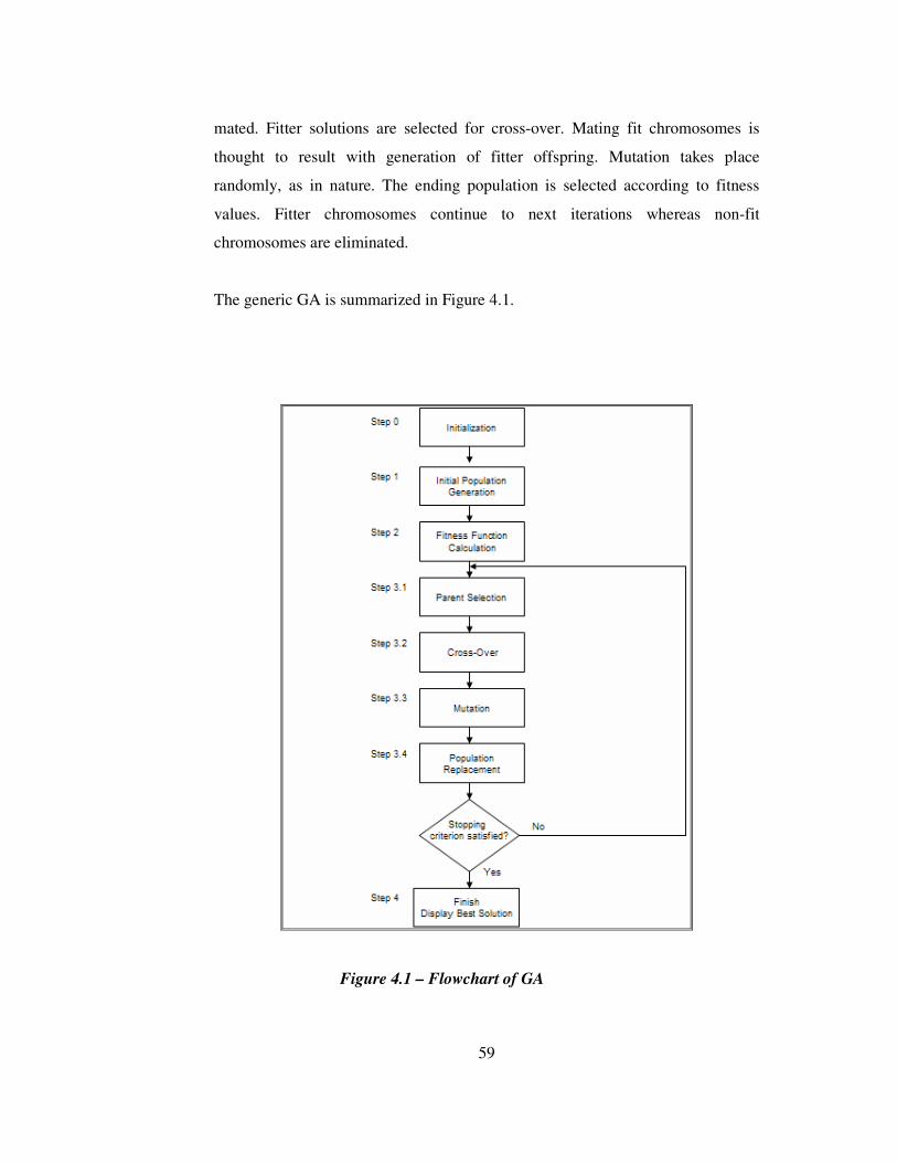
59

mated. Fitter solutions are selected for cross-over. Mating fit chromosomes is

thought to result with generation of fitter offspring. Mutation takes place

randomly, as in nature. The ending population is selected according to fitness

values. Fitter chromosomes continue to next iterations whereas non-fit

chromosomes are eliminated.

The generic GA is summarized in Figure 4.1.

Figure 4.1 – Flowchart of GA

60

Step 1. Initial Population Generation

The algorithm starts with an initial set of solutions which is called

population. The individual solutions are called chromosomes, and

the parts of chromosomes are called genes. Initial set of

chromosomes resemble Figure 4.2.

Figure 4.2 – Representation of initial set of chromosomes

Step 2. Fitness Function Computation

The chromosomes are evaluated according to their fitness values.

Fitness values represent the goodness of the solution. Fitness

function usually is the objective function. Slacks and surpluses of

61

unsatisfied constraints can be included as penalties.

Goodness of the solution specifies the probability of that solution to

persist in next generations.

Step 3. Evolution

The aim of the algorithm is converging the population average to

optimal solution of the search space. While a certain stopping

condition is not verified, the population evolves with the following

operations.

Step 3.1 Parent Selection

A mating pool is formed by selecting chromosomes of the

population according to their fitness values. Mating pool is

used to mate chromosomes which are called parent

chromosomes to generate child chromosomes which are

called offspring.

Selected parents are represented in Figure 4.3.

62

Figure 4.3 – Mating pool

Step 3.2 Cross-Over

Parent chromosome pairs merge by exchanging some of

their genes and generate offspring. The way of exchange is

determined by the cross-over strategy. Cross-over is

effective in exploring the search space.

Cross-overed chromosomes are shown in Figure 4.4.

63

Figure 4.4 – Chromosomes after cross-over

Step 3.3 Mutation

The chromosomes are subjected to mutation by either

modifying the chromosome completely or by modifying

some of the genes. The way of mutation is determined by the

mutation strategy. Mutation is effective in exploiting the

search space.

Mutated chromosomes are shown in Figure 4.5.

64

Figure 4.5 – Chromosomes after mutation

Step 3.4 Population Replacement

The offspring are replaced with the original population

according to a replacement strategy according to fitness

function values of the chromosomes. Resulting population

looks like Figure 4.6.

65

Figure 4.6 – Population after replacement

Step 4. Track of Best Solution

When the evolution procedure is finished, the best solution found so

far is displayed.

66

4.2 ALGORITHM DEVELOPMENT

4.2.1 CONSTRUCTION OF THE ALGORITHM

Each step of generic GA should be tuned in order to obtain a problem-specific

solver. As a starting point, representation of solutions carries a critical

importance.

Figure 4.7 – Encoding of solutions

In Figure 4.7, the chromosomes are represented as union of two separate gene

sets. The beginning gene set describes the nodes the health centers are opened

whereas the ending gene set describes the nodes the hospitals are opened. The

sizes of the gene sets are limited with the number of health centers-p and the

number of hospitals-q, sequentially. Thus, the size of the chromosome is p+q.

Since there is no restriction to open health centers and hospitals in the same node,

health center-gene set and hospital-gene set may contain same nodes. However,

67

opening more than one health centers/hospitals in the same node is prohibited.

This is ensured by repairs taking place in relevant steps of the algorithm.

Figure 4.8 – Representation of population

Numerous chromosomes form the population, as in Figure 4.8, which evolves

with cross-over, mutation and replacement throughout numerous iterations, as in

Figure 4.9. The numbers such as population size, cross-over rate, number of

iterations are left parametric during algorithm development. They attained their

final values after experiments.

68

.

.

.

Figure 4.9 – Evolution of population

population

cross-overed population

mutated population

iteration

69

4.2.2 STEPS OF THE ALGORITHM

The steps of the algorithm are summarized below.

Step 0. Initialization

Coverage matrices are calculated and time is started.

Coverage of demand at node Ii ∈ by health center at node

Jj ∈ ,

≥

≤≤−

−

≤

1

11

11

1

1

1

0

1

:cov

Tdistif

TdistSifST

distT

Sdistif

ij

ij

ij

ij

ij

Coverage of demand at node Ii ∈ by hospital at node Jj ∈ ,

≥

≤≤−

−

≤

2

22

22

2

2

2

0

1

:cov

Tdistif

TdistSifST

distT

Sdistif

ij

ij

ij

ij

ij

Coverage of health center at node Ji ∈ by hospital at node

Jj ∈ ,

≥

≤≤−

−

≤

3

33

33

3

3

3

0

1

:cov

Tdistif

TdistSifST

distT

Sdistif

ij

ij

ij

ij

ij

Coverage of demand at node Ji ∈ by health center at node

Jj ∈ ,

70

≥

≤≤−

−

≤

1

11

11

1

1

4

0

1

:cov

Tdistif

TdistSifST

distT

Sdistif

ij

ij

ij

ij

ij

Coverage of demand at node Ji ∈ by hospital at node Jj ∈ ,

≥

≤≤−

−

≤

2

22

22

2

2

5

0

1

:cov

Tdistif

TdistSifST

distT

Sdistif

ij

ij

ij

ij

ij

where

I denotes the set of demand points, J denotes the set of

potential facility sites; 1S denotes minimum critical distance of

demand-by-health center coverage, 2S denotes minimum critical

distance of demand-by-hospital coverage, 3S denotes minimum

critical distance of health center-by-hospital coverage; and 1T

denotes maximum critical distance of demand-by-health center

coverage, 2T denotes maximum critical distance of demand-by-

hospital coverage, 3T denotes maximum critical distance of

health center-by-hospital coverage.

Step 1. Generate initial population

Initial population is formed of two groups – initial population

that is generated totally randomly with ratio r1 and initial

population that is generated according to a heuristic or LP

relaxation with ratio r2, that is 1-r1.

Randomly generated initial population uses a random number

generator function to generate genes. Within p genes there is a

control to prevent repetition of opened health centers. In case of

repetition, the repeated gene is generated once more and control

71

starts from the beginning. The same control is performed within

next q genes. Since there is no restriction in opening a health

center and a hospital at the same place, controls are done

separately.

Heuristically generated population uses column sum of

coverages of all points having demand (demand points and

potential facility sites). Column sums are calculated as if points

are within critical distances of health centers, considering partial

coverage. The calculation is presented in Figure 4.10.

facility 1 facility 2 .. facility n

facility 1 .. coverage of demand at

node 1 by health center at

node 2

.. ..

facility 2 .. coverage of demand at

node 2 by health center at

node 2 .. ..

.. .. .. .. ..

facility n .. coverage of demand at

node n by health center at

node 2 .. ..

demand 1 .. coverage of demand at

node n+1 by health center

at node 2 .. ..

demand 2 .. coverage of demand at

node n+2 by health center

at node 2 .. ..

... .. .. .. ..

demand m .. coverage of demand at

node n+m by health center

at node 2 .. ..

column sum of facility 2

Figure 4.10 – Calculation of column sums

72

Column sum uses health center coverages only. There is no need

to include hospital coverages also, since health center coverage is

the strictest coverage. The column sums represent total closeness

of facilities to all nodes.

The facilities are column-sorted, the first p and q genes that give

the highest column-sums can be taken to form a chromosome.

Since the heuristic is deterministic, only one chromosome can be

generated this way. However, a number of chromosomes are

required to be generated. A probability factor is added as a

control in order to generate required number of chromosomes.

With %70 probability, the facility that has the highest column

sum is taken as the next gene. A random number is generated in

every iteration, if number is greater than 0.3, the next facility is

taken. If it is less than 0.3, the next facility is skipped. The total

number of genes allowed to be skipped is controlled by a

counter, since it is not preferable to skip more than possible

genes then start taking the same facilities from the beginning.

After the allowable limit, all facilities are sequentially included

in the chromosome. Same procedure is repeated for q genes.

There is another way to generate the non-random proportion; by

a heuristic that transfers the LP-relaxed solution to a feasible

integral solution set. The optimal LP-relaxed solution that is

obtained by GAMS, gives assignment of demand-health center,

demand-hospital, health center-hospital values and opened health

center values as non-integers between 0 and 1. The heuristic

forms sets for opened health centers and hospitals by taking the

non-zero valued health centers and hospitals to the sets and

neglecting others.

73

If the number of potential facility sites is 12, the number of

allowable hospitals is 4 and the corresponding GAMS output for

opened hospitals is as follows for instance;

z1 = 0.5 z2 = 0.33 z3 = 0.33 z4 = 0.33 z5 = 0.5 z6 = 0.4 z7 = 0 z8 = 0.4 z9 = 0.4 z10 = 0.4 z11 = 0 z12 = 0.4

Total opened hospitals = 4

where jz denotes whether it hosts a hospital or not at site j; then,

the relaxed hospital set is formed as {1, 2, 3, 4, 5, 6, 8, 9, 10, 12}

since the GAMS values for these potential sites are non-zero.

GAMS output is interpreted as the non-zero valued facilities

make a contribution to the coverage, but the zero-valued facilities

do not have any contribution. Therefore, the zero-valued

facilities are neglected in generating initial population.

The chromosomes are formed by selecting the genes from the

elements of the obtained relaxed health center and hospital sets

by a heuristic and this approach, in a way, lessens the feasible

region. In fact, our formulation does not include a variable set

that denote opened health centers. However, the opened health

centers can be found using demand-health center or health

center-hospital assignment values. The assignment values are

then transformed to opened health center and hospital values and

the relaxed health center set is obtained.

74

A probabilistic parameter controls the selection of the p genes of

chromosomes, from elements of the relaxed health center set.

The controlling parameter is

( )setcenterhealthrelaxedincentershealthofnumber

p−1 .

If the size of relaxed health center set is denoted by RHC , this

enables selection of p genes from RHC genes; where p is

always less than RHC by the constraints. The probability is

obliged to be greater than ||||

RHCpRHC − ; that is

genesofnumbertotalskippedbetogenesallowableofnumber

For instance, p is 10 and RHC is 50. Then the corresponding

controlling parameter is 0.8. If the generated random number is

greater than 0.8, the element of relaxed health center set is

included in the p genes and otherwise it is skipped.

The controlling parameter is selected so, in order to maintain a

balance for every condition of p and RHC . If the controlling

parameter was selected a fixed value at 0.5 for instance when p is

10 and RHC is 50, the number of skipped elements would be

small, and therefore the p genes of all chromosomes would

always be the beginning elements of relaxed health center set.

The ending elements would rarely be encountered to be included

in the take/skip decisions. By increasing number of skipped

elements, whole relaxed health center set is obliged to be

spanned and included in chromosomes.

75

If the number of skipped elements exceeds the number of

allowable elements to be skipped, all the next elements are

included in the chromosome. This also is controlled in every

skip.

The q genes are selected in the same way as the p genes. The

controlling parameter is sethospitalrelaxedofsize

q−1 .

Step 2. Calculate fitness functions

For all chromosomes, health centers and hospitals are

represented to be opened or unopened. In chromosome l, variable

1ljx is fixed at 1 if node j takes place in first p genes, and 0 if not.

Variable 2ljx is fixed at 1 if node j takes place in next q genes, and

0 otherwise. Variable 1x defines opened/unopened situation of a

health center, and 2x defines opened/unopened situation of a

hospital.

Demand Ii ∈ is tried to be assigned to health center-hospital

pairs first, in sequence. If health center Jj ∈ covers demand

Ii ∈ –if demand at Ii ∈ is within 1T distance of health center

at Jj ∈ – and hospital Jk ∈ covers health center Jj ∈ –if

health center at node Jj ∈ is within 3T distance of hospital at

node Jk ∈ –, demand is tried to be assigned to health center

Jj ∈ and then referred to hospital Jk ∈ . The fitness value is

calculated as

76

23111111 *cov**cov**cov* lkjkljijiljiji xxdemandxdemand +

where I denotes the set of demand points, J denotes the set of

potential facility sites; demand of node Ii ∈ is represented as

1idemand , coverage of demand Ii ∈ by health center Jj ∈ is

represented as 1covij , openness of health center Jj ∈ in

chromosome l is represented as 1ljx , coverage of health center

Jj ∈ by hospital Jk ∈ is represented as 3cov jk and openness of

hospital Jk ∈ in population l is represented as 2lkx .

If health center Jj ∈ can not cover demand Ii ∈ or hospital

Jk ∈ can not cover health center Jj ∈ , demand Ii ∈ is not

tried to be assigned to Jj ∈ .

After trying all feasible combinations of health center-hospital

pairs, demand is tried to be directly assigned to hospitals

sequentially, only if hospital Jk ∈ can cover demand Ii ∈ –

demand at node Ii ∈ is within 2T distance of hospital Jk ∈ –.

The fitness function is calculated as

221 *cov* ljiji xdemand


potential facility sites; demand of node Ii ∈ is represented as

1idemand , coverage of demand Ii ∈ by hospital Jj ∈ is

represented as 2cov ij , openness of hospital Jj ∈ in chromosome

l is represented as 2ljx .

77

From all the trials, the one with maximum fitness function is

selected for demand Ii ∈ .

Since the potential facility sites also possess demand, this

calculation is repeated for potential facility sites. Potential

facility site Ji ∈ is tried to be assigned to hospitals via health

centers first, with fitness value calculation of

23142142 *cov**cov**cov* lkjkljijiljiji xxdemandxdemand +


potential facility sites; demand of node Ji ∈ is represented as

2idemand , coverage of demand Ji ∈ by health center Jj ∈ is

represented as 4cov ij , openness of health center Jj ∈ in

chromosome l is represented as 1ljx , coverage of health center

Jj ∈ by hospital Jk ∈ is represented as 3cov jk and openness of

hospital Jk ∈ in population l is represented as 2lkx .

Then direct hospital assignments are considered with fitness

value calculation of

252 *cov* ljiji xdemand


potential facility sites; demand of node Ji ∈ is represented as

2idemand , coverage of demand Ji ∈ by hospital Jj ∈ is

represented as 5cov ij , openness of hospital Jj ∈ in chromosome

l is represented as 2ljx .

78

From all the trials, the one with maximum fitness function is

selected for demand at Ji ∈ . This is repeated for all nodes. Sum

of the fitness functions make up fitness function of chromosome

l. This is repeated for all chromosomes.

Step 3.1. Parent Selection

First the probabilities of selection for the mating pool are

calculated. Then parents are selected according to the

probabilities. Fitness ranking is a choice in order to prevent

domination of some particular chromosomes in the population. If

fitness ranking is applied probabilities are updated.

The probability of selecting chromosome k into the mating pool

is calculated by the following expression

minmax

min

fitnessfitness

fitnessfitnessprob k

k−

−=

where probability of selecting kth chromosome into the mating

pool is denoted by kprob , fitness value of chromosome k is

denoted by kfitness , minimum fitness value is denoted by

minfitness and maximum fitness value is denoted by maxfitness .

If fitness ranking is applied, fitness function values of

chromosomes are ranked. The rank of the chromosome with the

lowest fitness function value is assigned to 1. And as fitness

value is increased, rank is increased. Chromosomes with same

fitness value have same rank.

79

The probability of selecting chromosome k into the mating pool

is updated as follows

minmax

min

essrankedfitnessrankedfitn

essrankedfitnessrankedfitnprob k

k−

−=

where probability of selecting kth chromosome into the mating

pool is denoted by kprob , rank of chromosome k is denoted

bykessrankedfitn , minimum rank is denoted by

minessrankedfitn and maximum rank is denoted by

maxessrankedfitn .

Parents are selected according to the calculated kprob values, a

chromosome with a higher probability has more chance to be

selected as a parent. For chromosome k, a random probability is

generated. If kprob is greater than random variable,

chromosome k is included in the mating pool. Else, chromosome

k is skipped. This is repeated until mating pool is filled. In case

of skipping chromosomes such that chromosomes are finished

but mating pool is unfilled, the procedure continues with turning

back to the beginning chromosome. This allows including a

chromosome more than once in the mating pool. The mating pool

is kept.

Step 3.2. Cross-over

The consecutive chromosomes in the mating pool can be cross-

overed according to 4 strategies; 1-point cross-over, 2-point

cross-over, uniform mask cross-over and hybrid cross-over.

80

1-point cross-over is performed by changing middle genes of

consecutive chromosomes. Cutting points are selected as 2p

and 2q

p + in first p genes and next q genes, as presented şn

Figure 4.11.

Figure 4.11 – 1-point cross-over

2-point cross-over is performed by changing middle genes in

health center-hospital section of consecutive chromosomes.

Cutting points are selected as 3p , 3

2 p , 3q

p + and

32q

p + . 2-point cross-over is presented n Figure 4.12.

Figure 4.12 – 2-point cross-over

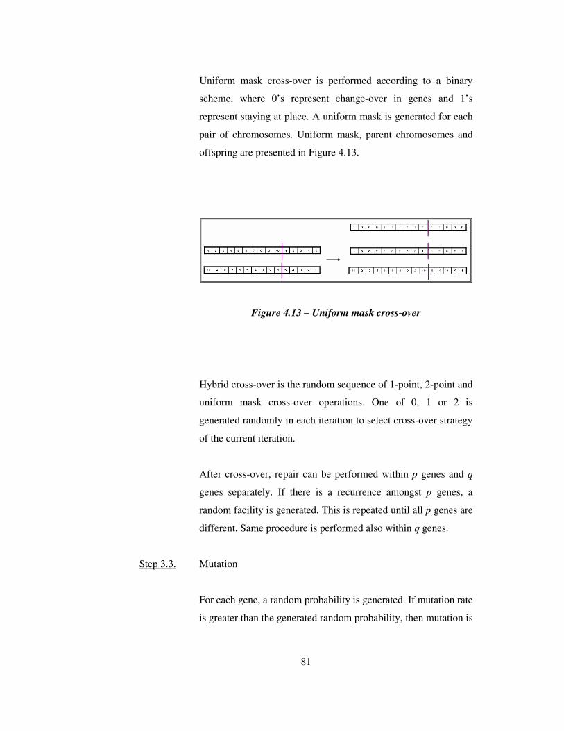
81

Uniform mask cross-over is performed according to a binary

scheme, where 0’s represent change-over in genes and 1’s

represent staying at place. A uniform mask is generated for each

pair of chromosomes. Uniform mask, parent chromosomes and

offspring are presented in Figure 4.13.

Figure 4.13 – Uniform mask cross-over

Hybrid cross-over is the random sequence of 1-point, 2-point and

uniform mask cross-over operations. One of 0, 1 or 2 is

generated randomly in each iteration to select cross-over strategy

of the current iteration.

After cross-over, repair can be performed within p genes and q

genes separately. If there is a recurrence amongst p genes, a

random facility is generated. This is repeated until all p genes are

different. Same procedure is performed also within q genes.

Step 3.3. Mutation

For each gene, a random probability is generated. If mutation rate

is greater than the generated random probability, then mutation is

82

performed on the gene. If not, the gene is kept as it is. Mutation

is performed by generating a random facility.

After mutation, repair can be performed within p genes and q

genes separately. If there is a recurrence amongst p genes, a

random facility is generated. This is repeated until all p genes are

different. Same procedure is performed also within q genes.

Step 3.4. Population replacement

There are 4 alternatives for population replacement;

unconditional replacement, unconditional replacement with

transfer of best solution, selection of best solutions amongst

original and offspring populations and conditional replacement.

Unconditional replacement is applied as below, Figure 4.14

represents it:

Replacement takes place before all operations. Chromosomes in

the mating pool take place of original chromosomes. If the size

of mating pool is less than the population size, last chromosomes

are remained as they are.

83

Figure 4.14 – Unconditional replacement

Unconditional replacement with transfer of best chromosome is

applied as below, Figure 4.15 represents it:

Replacement explained in Step 7a is performed. The difference

of transfer is adding the best chromosome of the last iteration to

the parent chromosomes of the current iteration. Best

chromosome is the chromosome with highest fitness function

value, that is caught anywhere of the iteration; it might be an

original chromosome, a chromosome with only cross-over or a

chromosome with both cross-over and mutation.

84

Figure 4.15 – Unconditional replacement with transfer

Best chromosome of the last iteration is inserted in a randomly

generated place of the population formed by unconditional

replacement explained above.

Selecting best of chromosomes in replacement

Offspring chromosomes are added to the original chromosomes

as in Figure 4.16.

85

Figure 4.16 – Addition of offspring chromosomes to parent

chromosomes

The formed enlarged population is sorted according to fitness

function values, as in Figure 4.17. The best population size of the

chromosomes are then selected and carried to the next iteration

as the original population, as in Figure 4.18.

86

Figure 4.17 – Sorting of enlarged population

Figure 4.18 – Selection of best of chromosomes amongst

sorted enlarged population

87

Replace cross-overed chromosomes with their parents if they are

fitter.

For each chromosome of the mating pool kept in Step 3.1, fitness

function values are calculated. Replacement of evolved

population with mating pool takes place. If fitness function of

evolved chromosome l is higher than its parent which is

chromosome l in the mating pool, evolved chromosome l is

replaced with chromosome l of mating pool. Otherwise,

chromosome l of mating pool endures to next generation.

After replacement, procedure starting with Step 3.1 is repeated

for number of iterations.

Step 4. Stop and display statistics.

Maximum fitness value, minimum fitness value, average fitness

value and the best gene of the ending population are kept. The

best fitness value of the population and solution time are also

kept.

4.3 STRATEGY SELECTION

GA, like other meta-heuristic algorithms, is a generic algorithm which has to be

pruned according to the specific characteristics of the problem. The methods and

rates for generation of new solutions have to be analyzed thoroughly to obtain a

good specific-to-problem algorithm.

The possible choices to prune are summarized in Table 4.1.

88

Table 4.1 – Possible choices for pruning the algorithm

Parameters Choices Generation of Population

Population Size 50 100 200 Initial Population Generation Ratios (Random - Non-

Random)

0.8 - 0.2 0.2 - 0.8

Non-Random Initial Population Generation Technique

heuristic LP-relaxation

Parent Selection Mating Pool

Selection with mating pool

selection without mating pool

selection

Fitness Ranking with ranking without ranking

Evolution

Cross-Over Operator 1-point cross-over 2-point cross-over uniform mask cross-

over random hybrid of cross-over types

Cross-Over Rate 0.8 1.0 Mutation Rate 0.01 0.05 0.1

Repair with repair without repair Number of Iterations 500 2000

Replacement

Replacement Method unconditional replacement

unconditional replacement with transfer of best solution of the

current generation to next generation

select best of sorted parent and offspring

chromosomes

replace offspring with their parents if

they are fitter

Replacement Sequence

before mutation after mutation

5 problems, whose caharacteristics are detailed in Table 4.2, are determined

randomly to compare the choices of the parameters. Preliminary experiments and

analyses are conducted to select the problem specific set of parameter values of

Table 4.1. These experiments and analyses are explained through steps i-vii.

89

Table 4.2 – Problems selected for preliminary analysis of strategy selection for

genetic algorithm

|I| |J| q p S1 S

2 S

3 T

1 T

2 T

3 w

1 w

2 w

3 δ

1 20 20 2 4 50 100 120 75 150 180 1 1 1 1

2 20 20 4 6 50 90 90 80 120 120 1 1 1 1

3 30 30 4 6 50 90 90 80 120 120 1 1 1 1

4 30 30 5 7 50 90 90 80 120 120 1 1 1 1

5 30 30 6 8 30 60 80 50 80 100 1 1 1 1

i) The first requirement that should be verified is thought to be the

evolution pattern of the GA. Evolution pattern suggests a course of

action on how well algorithm performs. Best solution of the algorithm

should draw an increasing pattern. The maximum fitness value should

also draw an increasing pattern while allowing deteriorations. Since

deteriorations help escaping from sub-optimals. The average fitness of

the population should converge to best fitness found so far to end

iterations.

The important parameters that affect the evolution pattern are the

method and sequence of replacement, the rate of mutation and the

decision of selection of mating pool. The patterns corresponding to

different combinations of these parameters are analyzed in Table 4.3.

5 problems indicated in Table 4.2 are solved with the different

combinations of parameters for each trial. The graphs drawn for the

problems of the same trial have different scales but similar patterns.

Thus, the graphs inserted below are representative of the patterns of

the statistical variables for the trials.

90

Table 4.3 – Analyses of GA patterns with respect to method and sequence of replacement, selection of mating pool and rate of

mutation

Trial Method of Replacement

Sequence of Replacement

Selection of Mating Pool

Rate of Mutation

Corresponding Pattern*

I 0.01 II 0.05 III

selected 0.1

IV 0.01 V 0.05 VI

Unconditional Replacement

sequence does not affect

not selected

0.1 VII 0.01 VIII 0.05 IX

selected

0.1 X 0.01 XI 0.05

XII

Unconditional Replacement with Transfer


not selected

0.1

0

100.000

200.000

300.000

400.000

500.000

600.000

700.000

800.000

0

99 198

297

396

495

594

693

792

891 990

1089

1188

1287

1386

1485

1584

1683

1782

1881

1980

f it_max

f it_avg

f it_min

best

XIII 0.01

XIV 0.05

XV

selected

0.1

XVI 0.01

XVII 0.05

XVIII

Select Best Solutions


not selected

0.1 0

100.000

200.000

300.000

400.000

500.000

600.000

700.000

0

93

18

6

27

9

37

2

46

5

55

8

65

1

74

4

83

7

93

0

10

23

11

16

12

09

13

02

13

95

14

88

15

81

16

74

17

67

18

60

19

53

fi t_max

fit_avg

fit_min

best

iteration

fitness

iteration

fitness

91

Table 4.3 (continued) – Analyses of GA patterns with respect to method and sequence of replacement, selection of mating pool

and rate of mutation




Rate of Mutation


XIX 0.01 XX 0.05

XXI selected

0.1

19.400.000

19.500.000

19.600.000

19.700.000

19.800.000

19.900.000

20.000.000

20.100.000

20.200.000

20.300.000

20.400.000

0

82

16

4

24

6

32

8

41

0

49

2

57

4

65

6

73

8

82

0

90

2

98

4

10

66

11

48

12

30

13

12

13

94

14

76

15

58

16

40

17

22

18

04

18

86

19

68

fi t_max

fi t_avg

fi t_min

best

XXII 0.01 XXIII 0.05

XXIV

Replace if Offspring Are

Fitter

after mutation

not selected

0.1

19.200.000

19.400.000

19.600.000

19.800.000

20.000.000

20.200.000

20.400.000

0

93

18

6

27

9

37

2

46

5

55

8

65

1

74

4

83

7

93

0

10

23

11

16

12

09

13

02

13

95

14

88

15

81

16

74

17

67

18

60

19

53

fi t_max

fit_avg

fit_min

bes t

iteration

iteration

fitness

fitness

92

Table 4.3 (continued) – Analyses of GA patterns with respect to method and sequence of replacement, selection of mating pool and

rate of mutation




Rate of Mutation


XXV 0.01

19.400.000

19.500.000

19.600.000

19.700.000

19.800.000

19.900.000

20.000.000

20.100.000

20.200.000

20.300.000

20.400.000

0

17

34

51

68

85

102

119

136

153

170

187

204

221

238

255

272

289

306

323

340

357

374

391

408

425

442

459

476

493

fit_max

fit_avg

fit_min

best

XXVI


Fitter

before mutation selected

0.05

19.400.000

19.500.000

19.600.000

19.700.000

19.800.000

19.900.000

20.000.000

20.100.000

20.200.000

20.300.000

0

17

34

51

68

85

102

119

136

153

170

187

204

221

238

255

272

289

306

323

340

357

374

391

408

425

442

459

476

493

fit_max

fit_avg

fit_min

best

iteration

iteration

fitness

fitness

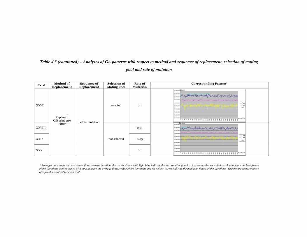
93

Table 4.3 (continued) – Analyses of GA patterns with respect to method and sequence of replacement, selection of mating

pool and rate of mutation




Rate of Mutation


XXVII selected 0.1

19.300.000

19.400.000

19.500.000

19.600.000

19.700.000

19.800.000

19.900.000

20.000.000

20.100.000

20.200.000

0

17

34

51

68

85

102

119

136

153

170

187

204

221

238

255

272

289

306

323

340

357

374

391

408

425

442

459

476

493

fit_max

fit_avg

fit_min

best

XXVIII 0.01

XXIX 0.05

XXX


Fitter

before mutation

not selected

0.1 19.300.000

19.400.000

19.500.000

19.600.000

19.700.000

19.800.000

19.900.000

20.000.000

20.100.000

20.200.000

0

17

34

51

68

85

102

119

136

153

170

187

204

221

238

255

272

289

306

323

340

357

374

391

408

425

442

459

476

493

fit_max

fit_avg

fit_min

best

* Amongst the graphs that are drawn fitness versus iteration, the curves drawn with light blue indicate the best solution found so far, curves drawn with dark blue indicate the best fitness

of the iterations, curves drawn with pink indicate the average fitness value of the iterations and the yellow curves indicate the minimum fitness of the iterations. Graphs are representative

of 5 problems solved for each trial.

iteration

iteration

fitness

fitness

94

Other parameters are kept constant as shown in Table 4.4 during the

trials.

Table 4.4 – Parameters kept constant during pattern selection runs


Population Size 100 Initial Population Generation Ratios (Random - Non-

Random)

0.8 - 0.2


heuristic

Parent Selection Fitness Ranking with ranking

Evolution Cross-Over Operator 1-point cross-over

Cross-Over Rate 0.8 Repair with repair

Number of Iterations 500

Amongst the trials I-XVIII, the method of replacement is the

determining factor. When the replacement method is unconditional

replacement with and without transfer of best gene to next iteration,

population average has an unstable evolution. It indicates no net

progress after some initial iterations since there exists no

convergence. The problem of non-developing population average is

solved when the replacement method is the selection of best solutions.

However, the desired graph is still not obtained. Population average

progresses but the progress is in company with progress of maximum

fitness of the current iteration and best fitness found so far. Population

average takes values a small amount less than the maximum fitness

95

values. This shows that most of the chromosomes resemble each

other in a short time. This brings premature convergence, which is

defined in literature as too early convergence of the population that

they could not evolve.

For the trials XIX-XXIV, replacing offspring with their parents

conditionally at the end is in question. If the mating pool is selected,

the evolution of population matches with the logic of GA, but the

entire statistical variables draw completely the same pattern a small

time after start; that is the diversity of the population vanishes. If the

mating pool is not selected, diversity is maintained, however

population average does not converge to best fitness. The lack of

natural selection takes these trials to non-convergence.

For the trials XXV-XXX that test replacing offspring conditionally

between cross-over and mutation, when mating pool is not selected;

the improvement in population average resembles the unconditional

replacement trials. The improvement is unstable. When mating pool is

selected, the mutation rate begins to be the determining factor. For the

rates 0.05 and 0.1 which would be categorized as large rates

according to literature, the population average indicates no net

improvement with unstable pattern.

Amongst all the trials, trial XXV satisfies all requirements; the

population average progresses and converges to best solution found so

far. On the other hand, the population maintains its diversity since

minimum fitness does not converge to best fitness and also alters

frequently.

The results indicate that ‘without mating pool selection’ choice of

mating pool selection parameter and ‘unconditional replacement,

96

‘unconditional replacement with transfer’ and ‘select best population’

choices of replacement scheme are eliminated.

ii) The second important factor that affects accuracy and rapidity of

progress, or in other words the gradient of the evolution curve is the

cross-over. Cross-over rate and method should be determined next.

With the replacement methods other than replace conditionally, the

cross-over rate would be considerably effective. However when the

replacement method is replace conditionally, in fact, the cross-over

rate becomes variable. If none of the offspring has better fitness values

than their parents, none will take place of their parents; thus it is

identical to having a cross-over rate of 0.0. If all individuals are cross-

overed and all offspring take place of their parents, then cross-over

rate is identical to 1.0. For the non-extreme cases, it always varies.

Therefore, keeping cross-over rate at 1.0 would provide maximum

opportunity.

Also, there is no loss by making more than required number of cross-

overs; since if the resulting offspring is not fit, it would not take place

of its parent. Therefore, cross-over rate is selected as 1.0.

Cross-over method is selected by experiments; that is the net effect of

change of cross-over operator is analyzed, other parameters being

constant as in Table 4.5. Each operator is tried on 5 problems of Table

4.2. Operators are compared in table 4.6.

97

Table 4.5 – Parameters kept constant to compare cross-over operators



Random)

0.8 - 0.2


heuristic



selection Fitness Ranking with ranking

Evolution Cross-Over Rate 1.0 Mutation Rate 0.01

Repair with repair Number of Iterations 500

Replacement

Replacement Method replace offspring

with their parents if they are fitter


before mutation

Table 4.6 – Comparison of cross-over operators

Statistics

Cross-Over Operator

Average of Deviations

from Optimal

Maximum of

Deviations from

Optimal

Variance of

Deviations From

Optimal

Average Time

(seconds)

1-point cross-

over 2.07% 3.92% 1.14% 7.2

2-point cross-over

0.34% 1.54% 0.67% 7.3

uniform mask cross-over

2.09% 4.58% 1.47% 6.9

hybrid cross-over

3.72% 5.20% 1.60% 7.4

98

2-point cross-over operator is more successful than other cross-over

operators. Thus, 1-point, uniform-mask and hybrid operators can be

eliminated.

iii) The next important determinant is the quality of starting generation.

The methods and ratios for generation of initial population are tested.

The quality and the diversity of the starting solution affect the

resulting solutions. For diversity, two trials are made. Problems of

Table 4.2 are solved with both combinations. The statistics of the

deviations of starting and ending solutions from optimal are

demonstrated in Table 4.8 while parameters kept constant are

demonstrated in Table 4.7.

Table 4.7 – Parameters kept constant to analyze effect of initial

population generation ratios



Random)

0.8 - 0.2


heuristic





Cross-Over Rate 1.0 Mutation Rate 0.01


Replacement




before mutation

99

Table 4.8 – Comparison of initial population generation

ratios

Statistics

Initial Population Generation Ratios

Deviation of Starting Solution

From Optimal

Deviation of Ending Solution From Optimal

Random: 0.2 –

Non-Random: 0.8 35.58% 0.24%

Random: 0.8 – Non-Random: 0.2

48.95% 5.43%

Results indicate that when the heuristically generated portion of initial

population is increased, the quality of starting population is increased.

Unless the randomly generated portion is decreased to 0.0, starting

with more qualified starting solutions result with lower deviations

from optimal.

If randomly generated proportion of the starting population vanishes,

the logic of GA that necessitates randomness to explore the search

space is violated. Thus, a random proportion is always required;

however starting with more qualified solutions is preferable. The ratios

are selected as 0.2-0.8 for random and non-random generation,

sequentially.

For comparing the method of generation of non-random starting

solutions, experiments are conducted on 5 problems of Table 4.2 for

both trials. Table 4.10 and 4.11 compare the results while Table 4.9

demonstrate the constatnt parameters during experiments .

100

Table 4.9 - Parameters kept constant to analyze method of generation of

non-random portion of initial solution



Random)

0.2 - 0.8







Replacement




before mutation

Table 4.10 – Comparison of non-random starting solution generation ratios

according to deviations of starting and ending solutions from optimal

Statistics Method of Generation for Non-Random

Portion of Starting Solution

Deviation of Starting Solution

From Optimal

Deviation of Ending Solution From Optimal

LP-Relaxation 26.16% 0.22%

Heuristic 35.58% 0.24%

101

Table 4.11 – Comparison of methods of non-random initial

population generation according to statistical values

Statistics Method of

Generation for Non-Random

Portion of Starting Solution


From Optimal

Maximum of Deviations

From Optimal

Variance of Deviations

From Optimal

Average Time to Generate

Initial Solution Set

(seconds)

LP-Relaxation 0.22% 3.42% 1.42% 3

Heuristic 0.24% 3.27% 1.86% 1

Both heuristics obtain similar and near-optimal results even though

LP-relaxation starts with about 10% better solutions. However, LP-

relaxation heuristic takes a larger time since the relaxed model is sent

to GAMS and the obtained optimal solution is taken back. Since,

there does not exist considerable difference in the quality, generation

of initial solution set with LP-relaxation heuristic is eliminated.

iv) It can be thought that repair is unnecessary, that GA would naturally

eliminate the chromosomes that include recurring genes in selection

phase; however when experiments are conducted, it is seen in Table

4.13 that repair makes a considerable effect. Table 4.12 presents the

parameters kept constant during experiments.

102

Table 4.12 – Parameters kept constant during analyses on effect of repair



Random)

0.2 - 0.8


heuristic






Number of Iterations 500

Replacement




before mutation

Table 4.13 – Analyses on effects of repair

Statistics

Repair of Chromosomes


From Optimal

Maximum of

Deviations From

Optimal


From Optimal

Average Time

(seconds) with repair 0.24% 0.84% 0.36% 7.3

without repair 6.42% 8.74% 1.72% 5.6

5 problems presented in Table 4.2 are solved with and without repair.

The statistical values demonstrate the average deviation, the

103

maximum deviation, the deviation variance and the average time for

the 5 problems. The additional time required after generation of initial

population, cross-over and mutation steps is inconsiderable when the

improvement repair performs is regarded. Thus, ‘without repair’

option is eliminated.

v) For fine tuning, the option of fitness ranking is evaluated. When

parents are not ranked, the differences in fitness values create

noteworthy differences in probabilities of selection for mating pool.

The effect of rank is analyzed through experiments on 5 problems

presented in Table 4.2. Table 4.15 summarizes the results where Table

4.14 demonstrates the paramtere kept constant during experiments.

Table 4.14 – Parameters kept constant during analyses on effect of fitness

ranking



Random)

0.2 - 0.8


heuristic



selection




Replacement




before mutation

104

Table 4.15 – Analyses on effects of fitness ranking

Statistics

Fitness Ranking


From Optimal

Maximum of

Deviations From

Optimal


From Optimal

Average Time

(seconds)

with ranking 0.24% 1.87% 0.89% 7.2

without ranking

5.79% 8.65% 2.79% 7.0

The effect of ranking worth the supplementary time required. The

patterns in Figure 4.19 indicate that not ranking lessens the population

diversity and brings premature convergence.

19.800.000

19.900.000

20.000.000

20.100.000

20.200.000

20.300.000

20.400.000

20.500.000

20.600.000

20.700.000

20.800.000

0

96

192

288

384

480

576

672

768

864

960

1056

1152

1248

1344

1440

1536

1632

1728

1824

1920

iterations

fitn

ess

fit_max

fit_avg

fit_min

best

Figure 4.19 – GA pattern when fitness ranking is skipped

105

Thus, ranking is preferred and not ranking option is eliminated.

vi) Population size is another parameter that has an effect on population

diversity. If population size is selected small, resemblance would

appear in most of the steps. In generation of initial population, small

population size would result with few randomly generated

chromosomes. This would reduce the power of randomness of GA. In

subsequent steps, since random chromosomes remain insufficient to

influence others, population would loose its diversity. On the other

hand, a two-fold large population size would take two-fold much time

computationally.

The trials for population sizes are evaluated in accordance with their

computational time requirements. Problems of Table 4.2 are solved

with each population size, results of which are tabulated in Table 4.17.

Table 4.16 shows parameters kept constant.

106

Table 4.16 – Parameters kept constant while analyzing the effect of

population sizes


Initial Population Generation Ratios (Random - Non-

Random)

0.2 - 0.8


heuristic







Replacement




before mutation

Table 4.17 – Comparison of population sizes

Statistics

Population Size


From Optimal

Maximum of

Deviations From

Optimal


From Optimal

Average Time

(seconds)

50 3.00% 4.65% 1.32% 3.5

100 0.30% 0.88% 0.35% 7.2

200 0.25% 0.88% 0.39% 14.1

107

Population size of 100 is considerably better than population size of

50, whereas the difference between the averages of deviations from

optimal can be neglected when the population sizes of 100 and 200 are

compared. On the other hand, solution times of population sizes of 100

and 200 are incomparable. Time difference can not be compensated

with the small improvement in average deviations and no

improvement in maximum deviations. Therefore, population size of

100 is selected.

vii) The last parameter that has to be taken into account with time

considerations is the iteration number. Initial runs have been made

using iteration number of 2000, however the graphs indicate that very

minor improvements take place after the iteration limit of 500. Figure

4.20 is presented below as a representative of all problems.

Figure 4.20 – Fitness vs. iteration graph to compare solution quality in 500 and

2000 iterations

The resulting problem-specific GA is then constituted from the parameter choices

summarized in Table 4.18.

108

Table 4.18 – Resulting GA strategy

Parameter Choice Selected in Step Generation of Population

Population Size 100 vi Initial Population Generation

Ratios (Random - Non-Random)

0.2 - 0.8 iii

Non-Random Initial Population Generation

Technique heuristic iii

Parent Selection Mating Pool Selection

with mating pool selection

i

Fitness Ranking with ranking v

Evolution Cross-Over Operator 2-point cross-over ii

Cross-Over Rate 1.0 ii Mutation Rate 0.01 i

Repair with repair iv Number of Iterations 500 vii

Replacement

Replacement Method replace offspring with their parents if they are

fitter i

Replacement Sequence before mutation i

4.4 ALGORITHM ON AN EXAMPLE PROBLEM

The steps of the pruned algorithm are illustrated on the example problem of

Section 3.6. Note that the sequence of steps 3.3 and 3.4 are exchanged and

replacement is performed before mutation in order to allow deterioration in the

population and prevent being stuck in sub-optimal solutions.

Parameters of the problem are re-represented in Table 4.19.

Table 4.19 – Example problem parameters for illustration of pruned GA

# of nodes

# of dema

nd nodes

# of potential facility

sites

# of

hospitals

# of health centers

S1 S2 S3 T1 T2 T3 w1 w2 w3 δ

50 - 50 6 14 30 60 80 50 80 100 1 1 1 1

109

Some chromosomes of the population are represented in Figures 4.21-4.32 to

illustrate the procedure in each step, for whole chromosomes Appendix D can be

seen.

Step 0. Initialize. Calculate coverage matrices and start clock.

Step 1. Generate initial population.

Step 1.1. Generate initial 20 chromosomes randomly. Repair

chromosomes.

Figure 4.21 – Repaired randomly generated initial

chromomes

Step 1.2. Generate initial 80 chromosomes using heuristic. Repair

chromosomes.

110

Figure 4.22 – Repaired heuristically generated initial

chromosomes

Step 2. Calculate fitness function values. Keep statistics.

Figure 4.23 – Fitness functions of initial population

Step 3. For 500 iterations, repeat.

Step 3.1. Select parents.

Step 3.1.1. Calculate probabilities to be selected for mating pool in the

presence of fitness ranking.

111

Step 3.1.2. Select parents.

Figure 4.24 – Parent chromosomes

Step 3.2. Cross-over.

Step 3.2.1. Perform 2-point cross-over.

Figure 4.25 – Cross-overed chromosomes (offspring)

Cross-over is performed between two consecutive parents by

112

exchange of genes between first and second and third and fourth

cutting points.

Step 3.2.2. Repair chromosomes.

Figure 4.26 – Repaired offspring

Step 3.2.3. Calculate fitness function values.

Figure 4.27 – Fitness function values of offspring population

Step 3.2.4. Keep statistics.

Step 3.3. Replace population.

113

Step 3.3.1. Calculate fitness function values of mating pool.

Figure 4.28 – Fitness function values of mating pool

Step 3.3.2. Replace offspring with parents if offspring are fitter.

Figure 4.29 – Resulting population after conditional replacement

of offspring with their parents

In Figure 4.29, the resulting population is presented. Offspring

chromosome 0 with fitness value of 348.99 is replaced with its

parent chromosome 0 which has a fitness value of 339.80. Offspring

114

chromosome 2 with fitness value of 178.17 does not take place of

its parent however, since parent chromosome 2 has a fitness value

of 244.22. Parent 0 is eliminated and offspring 0 is remained to next

generations whereas offspring 2 is eliminated and parent 2 is

remained to next generations.


Step 3.4. Mutate.

Step 3.4.1. Perform mutation.

Figure 4.30 – Mutated population

Since mutation rate is small, it is encountered rarely. In

chromosomes 0-3, no mutation takes place whereas in chromosome

10, two mutations take place.

Step 3.4.2. Repair chromosomes.

115

Figure 4.31 – Repaired mutated population

During mutation twelfth gene of chromosome 10 takes a recurring

value with sixth gene. It is repaired by generating a random facility.

Step 3.4.3. Calculate fitness function values.

Figure 4.32 – Fitness function values of ending population of

current iteration that will start to a new iteration


Step 4. End. Stop clock. Display results.

116

Statistics obtained from the first iteration are presented in Table

4.20. Statistics of all iterations are presented in Appendix D.

Table 4.20 – Results of first iteration

iteration maximum

fitness average fitness

minimum fitness

best fitness found so far

0 392.480 305.659 212.093 392.480

117

CHAPTER 5

Equation Section (Next)

5 COMPUTATIONAL EXPERIMENTS

A mixed-integer programming (MIP) model is constructed and a problem-specific

Genetic Algorithm (GA) is developed for the Hierarchical Maximum Covering

Location Problem (MCLP) with referral in presence of partial coverage

(HMCLP(R)-P). Since the problem has not been studied in literature before, it is

not possible to compare the results of the proposed GA with results of other

studies. For small problems, results are compared with optimal results and for

large problems, results are compared with the results of random heuristic that

chooses the best solution amongst a randomly generated solution set.

5.1 EXPERIMENTAL SETTINGS

The initial phase is the generation of problem instances. Different node sizes,

number of health centers, number of hospitals and different critical distances are

tried in each problem instance and 5 problems with different seeds are generated

for each instance. Problems are generated by generating x-coordinates uniformly

in the range 0 and 1000, y-coordinates uniformly in the range 0 and 500, and

demand weights for nodes uniformly in the range 1 and 20, in Visual C.

Euclidean distance metrics are utilized for calculation of intra-nodal distances.

Weights of objective function terms are taken as 1 to give equal importance to all

objectives and the rate of referral is taken as 1.

118

Table 5.1 – Tested problem instances

# of nodes

# of dema

nd nodes


sites

# of hospitals

# of health centers

S1 S2 S3 T1 T2 T3

2 4 50 100 120 75 150 180

3 5 50 90 90 80 120 120

20 - 20 4 6 50 90 90 80 120 120

30 - 30 3 5 50 90 90 80 120 120

4 6 50 90 90 80 120 120

5 7 50 90 90 80 120 120

6 8 30 60 80 50 80 100

40 - 40 4 8 50 90 90 80 120 120

4 12 50 90 90 80 120 120

6 12 30 60 80 50 80 100

6 14 30 60 80 50 80 100

50 - 50 4 12 50 90 90 80 120 120

6 12 30 60 80 50 80 100

6 14 30 60 80 50 80 100

8 16 30 60 80 50 80 100

60 - 60 6 12 50 90 90 80 120 120

6 14 50 90 90 80 120 120

8 16 50 90 90 80 120 120

10 20 30 50 80 80 75 120

250 200 50 5 10 50 90 90 80 120 120

10 15 30 60 80 50 80 100

500 450 50 5 10 50 90 90 80 120 120

10 15 30 60 80 50 80 100

400 100 5 10 50 90 90 80 120 120

10 15 20 60 60 30 90 90

20 30 10 50 50 15 75 75

1000 950 50 5 10 30 50 80 50 75 120

10 15 20 60 60 30 90 90

900 100 5 10 30 50 80 50 75 120

10 15 30 60 80 50 80 100

20 30 10 50 50 15 75 75

850 150 5 10 30 50 80 50 75 120

10 15 30 60 80 50 80 100

20 30 10 50 50 15 75 75

30 45

10 40 40 15 60 60

119

The critical distances are determined randomly but according to some basic rules

of thumb and utilizing the results of Section 3.6. These rules are given below.

• Minimum critical distance for coverage of demand by hospital ( 2S ) is

larger than minimum critical distance for coverage of demand by health

center ( 1S ),

• Minimum referral critical distance ( 3S ) is larger than or equal to minimum

critical distance for coverage of demand by hospital ( 2S ),

• Maximum critical distances are at least about 150% of minimum critical

distances

The problem instances are summarized in Table 5.1, while w1 = w

2 = w

3 =δ = 1.

The parameters such as the radii of critical distances, the number of health centers

and the number of hospitals determine the problem hardness when problems are

tried to be solved optimally. If the proportion of the total coverage area to the

total area is large, then the optimal configuration of facilities contains more

overlaps and this hardens and extends the Branch-and-Bound (B&B) procedure.

MIP models, presented in Appendices A and B, are solved using GAMS 19.6

with CPLEX solver. GA, pseudocode of which is presented in Appendix C, is

coded in Visual C. For comparisons, a random solver is also coded in Visual C.

The runs are conducted in a Pentium M Laptop with 1.86 GHz processor and 1

GB RAM.

5.2 RANDOM HEURISTIC

Random heuristic that generates a set of random solutions and takes the best

solution amongst all is developed. The same procedure that is used for generation

of random proportion of initial population of GA is applied without repair phase.

120

For determination of number of random solutions to be generated, experiments

are conducted. Table 5.3 compares the changes in solution quality and required

time for different number of solutions, which are tested on the problem set

presented in Table 5.2.

Table 5.2 – Test problems for random heuristic

|I| |J| q p S1 S

2 S

3 T

1 T

2 T

3 w

1 w

2 w

3 δ

1 20 20 3 5 50 90 90 80 120 120 1 1 1 1

2 20 20 4 6 50 90 90 80 120 120 1 1 1 1

3 30 30 3 5 50 90 90 80 120 120 1 1 1 1

4 30 30 4 6 50 90 90 80 120 120 1 1 1 1

5 30 30 5 7 50 90 90 80 120 120 1 1 1 1

Table 5.3 – Changes in solution quality and time with increasing iterations

5000 iterations vs.

10000 iterations

10000 iterations vs. 20000 iterations



30000 iterations vs.

40000 iterations


50000 iterations

vs. 100000 iterations

Average of Improvements

0,72% 0,67% 0,54% 0,00% 0,06% 0,06% 0,09%

Average Difference in Runtimes (sec.)

0,11 0,15 0,11 0,10 0,15 0,17 0,86

The number of solutions to be generated is selected as 25000, considering

solution quality and time requirement trade-off.

121

5.3 RESULTS

For problem sizes up to 50 nodes, optimal results could be obtained by GAMS

and GA results are compared with GAMS results. For problem sizes of more than

50 nodes, GAMS could not find solution in 3600 seconds although depth-first

search and putting bounds on variable strategies are tried. Large problems are

compared with random heuristic results.

The results in Table 5.4 indicate that the GA finds solutions with maximum of 5%

deviation from optimal results on the average. The amounts of deviations seem to

follow a generally increasing pattern with increase of problem size which is

expected, however the increase is very small. There is a higher increase in

maximum deviations which indicate that increase in problem size brings increase

in variance.

When compared with random heuristic, GA creates difference about 20% in

average, especially when the problem sizes increase.

When time requirements are considered as in Table 5.5, GAMS requires highly

varying times according to the complexity of the problem. For problems of size

60 nodes and larger, it was not possible to find solutions in 3600 seconds. GA,

however, is not affected from the problem complexity since the logic is the

exploration – exploitation of the search space which takes constant computation

time for the same problem sizes. Also, the time requirements are certainly

acceptable when quality of solutions is regarded. The time requirement to solve a

problem of size 1000 nodes is at most 7 minutes.

122

Table 5.4 – Results of GA compared with optimal and random solutions

(Optimal-GA Result)/Optimal (GA Result-Random)/Random

# of Nodes

# of Demand Nodes

# of Potential Facility

Sites

# of

Hospitals

# of Health Centers


Minimum of

Deviations

Maximum of

Deviations


# of Optimals Found by

GA


Minimum of

Deviations

Maximum of Deviations


20 - 20 2 4 0.00% 0.00% 0.01% 0.00% 4 4.38% 0.00% 9.49% 3.58% 3 5 1.45% 0.00% 6.04% 2.61% 1 4.74% 1.83% 8.96% 2.86% 4 6 0.19% 0.00% 0.89% 0.39% 3 9.54% 4.08% 13.63% 3.52%

30 - 30 3 5 2.99% 0.00% 10.17% 4.22% 2 10.66% 1.55% 17.42% 6.07% 4 6 1.60% 0.00% 4.33% 1.78% 1 12.00% 7.51% 15.98% 3.71% 5 7 0.08% 0.00% 0.38% 0.17% 3 14.29% 10.34% 16.40% 2.42% 6 8 0.87% 0.00% 1.87% 0.87% 2 18.83% 12.61% 25.38% 4.71%

40 - 40 4 8 1.65% 0.00% 3.74% 1.68% 1 19.50% 14.60% 23.80% 3.37% 4 12 3.45% 0.31% 4.89% 1.85% 0 17.30% 8.85% 23.64% 6.08% 6 12 1.91% 0.00% 6.39% 2.56% 0 23.04% 19.31% 25.06% 2.22% 6 14 1.90% 0.00% 4.73% 2.29% 1 21.59% 17.99% 24.08% 2.29%

50 - 50 4 12 * 4.19% 1.47% 7.42% 2.50% 0 21.36% 17.90% 25.59% 3.17% 6 12 1.77% 0.53% 4.17% 1.50% 0 27.02% 23.50% 31.96% 3.37% 6 14 4.49% 2.08% 8.74% 2.62% 0 24.38% 20.55% 28.00% 2.67% 8 16 3.23% 0.04% 6.71% 2.37% 0 25.11% 22.06% 27.50% 2.26%

60 - 60 6 12 ** 5.70% 5.70% 5.70% 5.70% 0 22.80% 21.76% 23.90% 0.94% 6 14 *** - - - - - 23.31% 20.90% 27.03% 2.27% 8 16 *** - - - - - 22.09% 18.11% 24.12% 2.37% 10 20 *** - - - - - 24.67% 23.10% 28.74% 2.33%

123

Table 5.4 (continued) – Results of GA compared with optimal and random solutions

(Optimal-GA Result)/Optimal (GA Result-Random)/Random

# of Nodes

# of Demand Nodes


Sites

# of

Hospitals

# of Health Centers


Minimum of Deviations

Maximum of

Deviations


# of Optimals Found by

GA


Minimum of

Deviations

Maximum of

Deviations


250 200 50 5 10 *** - - - - - 21.81% 19.33% 24.75% 2.22% 10 15 *** - - - - - 23.08% 18.19% 25.40% 2.88%

500 450 50 5 10 *** - - - - - 21.57% 15.29% 25.71% 3.84% 10 15 *** - - - - - 22.05% 19.92% 24.41% 1.70% 400 100 5 10 *** - - - - - 24.41% 20.56% 27.33% 2.52% 10 15 *** - - - - - 23.78% 21.20% 26.47% 2.06% 20 30 *** - - - - - 22.81% 20.85% 24.84% 1.48%

1000 950 50 5 10 *** - - - - - 20.92% 18.25% 24.06% 2.31% 10 15 *** - - - - - 15.95% 14.83% 19.05% 1.75% 900 100 5 10 *** - - - - - 22.36% 19.38% 25.43% 2.90% 10 15 *** - - - - - 25.49% 22.41% 28.80% 2.37% 20 30 *** - - - - - 20.48% 19.24% 21.92% 1.30% 850 150 5 10 *** - - - - - 27.50% 21.95% 33.25% 4.87% 10 15 *** - - - - - 25.82% 22.94% 27.51% 1.87% 20 30 *** - - - - - 22.06% 20.56% 23.96% 1.34% 30 45 *** - - - - - 25.18% 23.03% 27.23% 1.99%

* 1 of 5 problems could not be solved in 3600 sec. The statistics are calculated amongst 4 problems.

** Only 1 of 5 problems could be solved in 3600 seconds by introducing lower bound on the objective function variable.

*** None of the problems could be solved optimally in 3600 seconds.

124

Table 5.5 – Computational time requirements of GA compared with GAMS CPLEX and random heuristic

GAMS Time (seconds) GA Time (seconds) Random Time (seconds)

# of Nodes

# of Demand Nodes


Sites

# of

Hospitals

# of Health Centers

Avg Time Min Time

Max Time

Variance in Time

Avg Time

Min Time

Max Time

Variance in Time

Avg Time

Min Time

Max Time

Variance in Time

2 4 0.08 0.06 0.09 0.01 1.76 1.67 1.88 0.08 0.36 0.33 0.42 0.04 3 5 0.56 0.05 1.55 0.70 1.79 1.65 1.88 0.09 0.35 0.27 0.42 0.06

20 - 20 4 6 0.22 0.06 0.80 0.32 2.01 1.91 2.14 0.10 0.43 0.38 0.50 0.05

30 - 30 3 5 1.80 0.03 5.10 2.43 3.41 3.27 3.59 0.13 0.61 0.55 0.66 0.04 4 6 7.27 0.08 21.63 8.72 3.54 3.27 3.88 0.23 0.64 0.59 0.67 0.03 5 7 5.68 0.13 19.06 7.69 3.81 3.69 4.05 0.15 0.68 0.61 0.75 0.05 6 8 0.08 0.08 0.11 0.01 3.63 3.47 3.75 0.11 0.67 0.64 0.69 0.02

40 - 40 4 8 41.59 13.89 109.47 39.28 6.17 6.06 6.36 0.11 1.00 0.92 1.05 0.05 4 12 354.03 5.41 1615.20 706.87 7.00 6.69 7.34 0.27 1.09 1.08 1.11 0.02 6 12 0.39 0.09 1.58 0.66 6.29 6.06 6.39 0.13 1.04 1.00 1.08 0.03 6 14 33.74 1.00 115.42 47.70 6.80 6.41 6.97 0.23 1.11 1.08 1.13 0.02

50 - 50 4 12 * 1377.53 212.97 2936.53 1240.05 10.02 9.61 10.36 0.27 1.50 1.42 1.55 0.05 6 12 8.12 2.11 28.23 11.26 9.06 8.84 9.52 0.27 1.44 1.41 1.45 0.02 6 14 30.59 1.00 146.55 64.83 9.34 9.14 9.55 0.20 1.47 1.39 1.50 0.05 8 16 266.67 1.00 1087.72 466.43 9.86 9.58 10.20 0.29 1.54 1.52 1.56 0.02

60 - 60 6 12 ** 1837.44 1837.44 1837.44 1837.44 13.83 13.53 14.16 0.25 2.07 2.00 2.24 0.10 6 14 *** - - - - 14.34 14.03 14.53 0.21 2.21 2.13 2.27 0.06 8 16 *** - - - - 14.85 14.50 15.27 0.35 2.29 2.16 2.36 0.08 10 20 *** - - - - 16.12 15.56 16.70 0.44 2.52 2.44 2.61 0.06

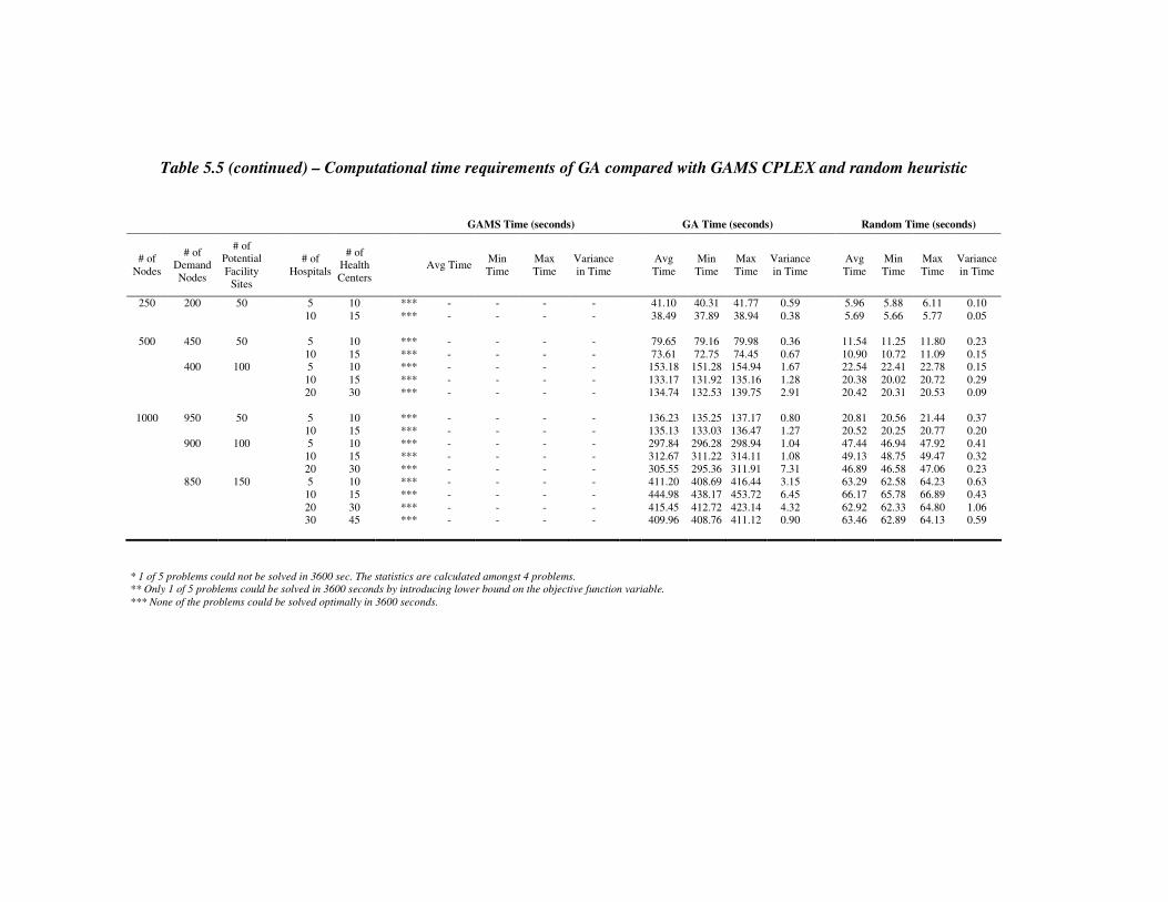
125

Table 5.5 (continued) – Computational time requirements of GA compared with GAMS CPLEX and random heuristic

GAMS Time (seconds) GA Time (seconds) Random Time (seconds)

# of Nodes

# of Demand Nodes


Sites

# of

Hospitals

# of Health Centers

Avg Time Min Time

Max Time

Variance in Time

Avg Time

Min Time

Max Time

Variance in Time

Avg Time

Min Time

Max Time

Variance in Time

250 200 50 5 10 *** - - - - 41.10 40.31 41.77 0.59 5.96 5.88 6.11 0.10 10 15 *** - - - - 38.49 37.89 38.94 0.38 5.69 5.66 5.77 0.05

500 450 50 5 10 *** - - - - 79.65 79.16 79.98 0.36 11.54 11.25 11.80 0.23 10 15 *** - - - - 73.61 72.75 74.45 0.67 10.90 10.72 11.09 0.15 400 100 5 10 *** - - - - 153.18 151.28 154.94 1.67 22.54 22.41 22.78 0.15 10 15 *** - - - - 133.17 131.92 135.16 1.28 20.38 20.02 20.72 0.29 20 30 *** - - - - 134.74 132.53 139.75 2.91 20.42 20.31 20.53 0.09

1000 950 50 5 10 *** - - - - 136.23 135.25 137.17 0.80 20.81 20.56 21.44 0.37 10 15 *** - - - - 135.13 133.03 136.47 1.27 20.52 20.25 20.77 0.20 900 100 5 10 *** - - - - 297.84 296.28 298.94 1.04 47.44 46.94 47.92 0.41 10 15 *** - - - - 312.67 311.22 314.11 1.08 49.13 48.75 49.47 0.32 20 30 *** - - - - 305.55 295.36 311.91 7.31 46.89 46.58 47.06 0.23 850 150 5 10 *** - - - - 411.20 408.69 416.44 3.15 63.29 62.58 64.23 0.63 10 15 *** - - - - 444.98 438.17 453.72 6.45 66.17 65.78 66.89 0.43 20 30 *** - - - - 415.45 412.72 423.14 4.32 62.92 62.33 64.80 1.06 30 45 *** - - - - 409.96 408.76 411.12 0.90 63.46 62.89 64.13 0.59

* 1 of 5 problems could not be solved in 3600 sec. The statistics are calculated amongst 4 problems.

** Only 1 of 5 problems could be solved in 3600 seconds by introducing lower bound on the objective function variable.

*** None of the problems could be solved optimally in 3600 seconds.

126

CHAPTER 6

6 CONCLUSION AND FUTURE RESEARCH

We combined HCMLP, referral and MCLP-P, and proposed a HMCLP(R)-P

formulation to model the requirements of health systems more realistically.

Proposed formulation has several extensions to classical HMCLP with different

combination of characteristics: (i) 3 types of demand –demand requiring low-

level service, demand requiring high-level service and demand requiring both

levels of service at the same time- is considered but all demand of a demand point

is covered as a whole. (ii) We considered a successively inclusive hierarchy and

referral to meet the 3 types of demand requirement at once. (iii) We integrated

partial coverage to HMCLP.

Integration of partial coverage increases the complexity of the problem. In

classical MCLP’s and HMCLP’s, the information of which facility covers which

demand is not important. The important notion is the coverage and whether a

demand point can be covered or not. However, integration of partial coverage

brings assignment to HMCLP(R)-P, since calculation of partial coverage requires

information of distance between nodes. Thus, the NP-hard HMCLP becomes even

harder to solve.

We proposed a MIP formulation and tried to find optimal results using GAMS

19.6 with CPLEX solver. GAMS was able to solve problems up to size of 50

nodes within a time limit of 3600 seconds. For the problems of larger scale,

frequently used time-reducing methods such as modifying the B&B strategy to

127

depth-first search or putting bounds on variables to accelerate fathoming of B&B

procedure were even not of use.

We proposed a problem-specific GA that is fast and produces near-optimal results

for large-size problems. The algorithm has pruned its final state after initial

experiments for eah strategy. It is tested on problems of sizes 20 to 1000 nodes

and compared with optimal solutions for small-sized and with random solutions

for large-sized problems. The deviations and time requirements are reasonable.

Even though MCLP has been studied widely, it can be extended on several

directions. HMCLP is one of those extensions. We developed and proposed a

solution procedure. A future research direction would be developing heuristics or

applying other meta-heuristics to HMCLP(R)-P, such as Simulated Annealing and

Tabu Search.

Another future research might be studying the capacitated version of HMCLP(R)-

P. Since we already included assignments, introduction of capacity would not

require additional variables but only additional constraints.

128

REFERENCES

Beasley, J. E., Bull, D. R. & Martin, R. R. (1993). An Overview of Genetic

Algorithms: Part I Fundamentals. University Comp, 15, 170-181.

Beasley, J. E. & Chu, P. C. (1996). A Genetic Algorithm for the Set Covering

Problem. European Journal of Operational Research, 94, 392-404.

Berman, O. & Krass, D. (2002). The Generalized Maximal Covering Location

Problem. Computers & Operations Research, 29, 563-581.

Berman, O., Krass, D. & Drezner, Z. (2003). The Gradual Covering Decay

Location Problem On A Network. European Journal of Operational Research,

151, 474-480.

Charnes, A. & Storbeck, J. (1980). A Goal Programming Model for the Siting of

Multilevel EMS Systems. Socio-Econ. Plan. Sci., 14, 155-161.

Chung, C-H. (1986). Recent Applications of the Maximal Covering Location

Planning (M.C.L.P.) Model. J. Opl. Res. Soc., 37(8), 735-746.

Church, R. & ReVelle, C. (1974). The Maximal Covering Location Problem.

Papers of the Regional Science Association, 32, 101-118.

Drezner, Z., Wesolowsky, G. O., & Drezner, T. (2004). The Gradual Covering

Problem. Naval Research Logistics, 51, 841-855.

129

Eitan, Y., Narula, S.C. & Tien, J. M. (1991). A Generalized Approach to

Modeling the Hierarchical Location-Allocation Problem. IEEE Transactions on

Systems, Man and Cybernetics, 21(1), 39-46.

Espejo, L. G. A., Galvão, R. D. & Boffey, B. (2003). Dual-Based Heuristics for a

Hierarchical Covering Location Problem. Computers & Operations Research, 30,

165-180.

Goldberg, D. E. (1989). Genetic Algorithms in Search, Optimization and Machine

Learning. Reading, MA: Addison-Wesley.

Holland, J. (1975). Adaptation in Natural and Artificial Systems. Univ. of

Michigan Press, Ann Arbor, MI.

Karasakal, O. & Karasakal, E. (2004). A Maximal Covering Location Model in

The Presence of Partial Coverage. Computers & Operations Research, 31, 1515-

1526.

Li, X. & Yeh, A. G. (2004). Integration of Genetic Algorithms and GIS for

Optimal Location Search. International Journal of Geographical Information

Science. 19(5), 581-601.

Marianov, V. & Serra, D. (2001). Hierarchical Location-Allocation Models for

Congested Systems. European Journal of Operational Research, 135, 195-208.

Moore, G. C. & ReVelle, C. (1982). The Hierarchical Service Location Problem.

Management Science, 28(7), 775-780.

Narula, S. C. & Ogbu, U. I. (1978). An Hierarchical Location-Allocation

Problem. OMEGA. The Int. Jl of Mgmt. Sci., 7(2), 137-143.

130

Narula, S. C. & Ogbu, U. I. (1984). Lagrangean Relaxation and Decomposition in

an Uncapacitated 2-Hierarchical Location-Allocation Problem. Computers &

Operations Research, 12(2), 169-180.

Şahin, G. & Süral, H. (2007). A Review of Hierarchical Facility Location Models.

Computers & Operations Research, 34, 2310-2331.

Toregas, C., Swain, R., ReVelle, C. & Bergman, L. (1971). The Location of

Emergency Service Facilities. Operations Research, 19, 1363-1373.

Töreyen, Ö., Karasakal, E. & Karasakal, O. (2006). Hierarchical Maximal

Covering Location Problem with Referral in Presence of Partial Coverage.

Presented at the 26th

National Operations Research and Industrial Engineering

Congress 2006, Kocaeli, Turkey.

131

APPENDIX A

A GAMS FORMULATION 1

sets

i nodes /1*50/;

alias (i,j);

alias (i,k);

parameters d(i) demand matrix

$include "C:\Documents and

Settings\oz_tez\gams_bastan\book41.txt";

table dist(i,j) distance between nodes i and j



parameter s1 critical distance1;

s1 = 30;

parameter t1 critical distance2;

t1 = 50;


s2 = 60;


t2 = 80;


s3 = 80;


t3 = 100;

parameter a1(i,j) binary coverage (T1) of demand i by

health center at j;

a1(i,j) = 0;

a1(i,j)$(dist(i,j) ne t1) = (1 + (1- (dist(i,j) / t1)) /

abs(1 - (dist(i,j) /t1))) / 2;

parameter a2(i,j) binary coverage (T2) of demand at i

hospital at j;

132

a2(i,j) = 0;


abs(1 - (dist(i,j) /t2))) / 2;

parameter a3(i,j) binary coverage (T3) of health center

at i by hospital at j;

a3(i,j) = 0;


abs(1 - (dist(i,j) /t3))) / 2;

parameter c1(i,j) partial coverage of demand i by health

center at j;

c1(i,j) = min(1 , max(0 , (t1 - dist(i,j)) / (t1-s1)));

parameter c2(i,j) partial coverage of demand at i

hospital at j;


parameter c3(i,j) partial coverage of health center at i

by hospital at j;


sets

m1(i,j) first coverage

m2(i,j) second coverage

m3(i,j) hospital coverage;

m1(i,j)=no;

m2(i,j)=no;

m3(i,j)=no;

m1(i,j)$(a1(i,j) eq 1)=yes;



binary variables

x1(i,j) if demand at i is assigned to health

center at j

x2(i,j) if demand at i is assigned to hospital at

j

y(i,j) if health center at i is opened and

assigned to hospital at j

z(j) if hospital is opened at j ;

positive variables

u(j,k) demand in health center j that is covered

by hospital k ;

variable t objective function value ;

equations

133

obj objective function

numfac1 number of hospitals limited to q

numfac2 number of health centers limited

to p

cov1(i,j) demand-health center coverage

cov2(i,j) demand-hospital coverage

cov3(i,j) health center-hospital coverage

ass1(i) demand-health center and hospital

assignment

ass2(i) health center-hospital assignment

lin1(j,k) linearization1

lin2(j,k) linearization2;

obj.. t =e= sum((i,j)$m1(i,j),

d(i)*c1(i,j)*x1(i,j))+sum((i,j)$m2(i,j)

,d(i)*c2(i,j)*x2(i,j))+sum((j,k)$m3(j,k), u(j,k));

numfac1.. sum(j,z(j)) =e= 6;

numfac2.. sum((i,j)$m3(i,j),y(i,j)) =l= 14;

cov1(i,j)$m1(i,j).. x1(i,j) =l= sum(k$(a3(j,k) eq

1),y(j,k));

cov2(i,j)$m2(i,j).. x2(i,j) =l= z(j);

cov3(i,j)$m3(i,j).. y(i,j) =l= z(j);

ass1(i).. sum(j$(a1(i,j) eq

1),x1(i,j))+sum(j$(a2(i,j) eq 1),x2(i,j)) =l= 1;

ass2(i).. sum(j$(a3(i,j) eq 1),y(i,j)) =l=

1;

lin1(j,k)$m3(j,k).. u(j,k) =l= sum(i$(a1(i,j) eq

1),d(i)*c1(i,j)*x1(i,j))*c3(j,k);

lin2(j,k)$m3(j,k).. u(j,k) =l= 1000*y(j,k);

model oz /all/;

OPTIONS LIMROW=200, LIMCOL=200, SYSOUT=OFF, SOLPRINT=ON,

ITERLIM=2000000, RESLIM=40800, optcr=0.0, BRATIO=0,

MIP=cplex;

solve oz using mip maximizing t;

display x1.l, x1.m, x2.l, x2.m, y.l, y.m, z.l, z.m, u.l,

u.m;

134

APPENDIX B

B GAMS FORMULATION 2

sets

i nodes /1*20/;

alias (i,j);

alias (i,k);

parameters d(i) demand matrix



table dist(i,j) distance between nodes i and j




s1 = 10;


t1 = 20;


s2 = 20;


t2 = 40;


s3 = 25;


t3 = 50;

parameter a1(i,j) binary coverage (T1) of demand i by

health center at j;

a1(i,j) = 0;


abs(1 - (dist(i,j) /t1))) / 2;

parameter a2(i,j) binary coverage (T2) of demand at i

hospital at j;

a2(i,j) = 0;


abs(1 - (dist(i,j) /t2))) / 2;

135

parameter a3(i,j) binary coverage (T3) of health center

at i by hospital at j;

a3(i,j) = 0;


abs(1 - (dist(i,j) /t3))) / 2;

parameter c1(i,j) partial coverage of demand i by health

center at j;


parameter c2(i,j) partial coverage of demand at i

hospital at j;


parameter c3(i,j) partial coverage of health center at i

by hospital at j;


sets

m1(i,j) first coverage

m2(i,j) second coverage

m3(i,j) hospital coverage;

m1(i,j)=no;

m2(i,j)=no;

m3(i,j)=no;




binary variables

x1(i,j) if demand at i is assigned to health

center at j

x2(i,j) if demand at i is assigned to hospital at

j

y(i,j) if health center at i is opened and

assigned to hospital at j

z(j) if hospital is opened at j

u(i,j,k) if demand i is assigned to health center

j and health center j is assigned to hospital k ;

variable t objective function value;

equations

obj objective function

numfac1 number of hospitals limited to p

numfac2 number of health centers limited

to q

cov1(i,j) demand-health center coverage

136

cov2(i,j) demand-hospital coverage

cov3(i,j) health center-hospital coverage

ass1(i) demand-health center and hospital

assignment

ass2(i) health center-hospital assignment

lin(i,j,k) linearization;

obj.. t =e=

sum((i,j)$m1(i,j),d(i)*c1(i,j)*x1(i,j))+sum((i,j)$m2(i,j),d

(i)*c2(i,j)*x2(i,j))+sum((i,j,k)$(m1(i,j) and

m3(j,k)),d(i)*c1(i,j)*c3(j,k)*u(i,j,k));

numfac1.. sum(j,z(j)) =e= 4;

numfac2..

sum((i,j)$m3(i,j),y(i,j)) =l= 6;

cov1(i,j)$m1(i,j).. x1(i,j) =l=

sum(k$(a3(j,k) eq 1),y(j,k));

cov2(i,j)$m2(i,j).. x2(i,j) =l= z(j);

cov3(i,j)$m3(i,j).. y(i,j) =l= z(j);


1),x1(i,j))+sum(j$(a2(i,j) eq 1),x2(i,j)) =l= 1;


1),y(i,j)) =l= 1;

lin(i,j,k)$(m1(i,j) and m3(j,k)).. u(i,j,k) =l=

0.5*x1(i,j)+0.5*y(j,k);

model oz /all/;

OPTIONS LIMROW=0, LIMCOL=0, SYSOUT=OFF, SOLPRINT=ON,

ITERLIM=2000000, RESLIM=40800, optcr=0.0, BRATIO=0,

MIP=cplex;

solve oz using mip maximizing t;

display x1.l, x1.m, x2.l, x2.m, y.l, y.m, z.l, z.m, u.l,

u.m;

137

APPENDIX C

C GA PSEUDOCODE

0 generate problem

0.1 distance1 (from demand nodes to potential facility nodes) matrix

generation

0.2 for i=1 to num_dem, repeat

0.3 for j=1 to num_fac, repeat

0.4 generate distance1[i,j] ← random

distances~Uniform[1,200] using

lcgrand function

0.5 distance2 (between potential facility nodes) matrix generation

0.6 for i=1 to num_fac, repeat

0.7 diagonal is 0

0.8 for j=1 to num_fac (upper tringle), repeat

0.9 generate distance2[i,j] ← random

distances~Uniform[1,200] using

lcgrand function

0.10 take lower triangle symmetric with

upper triangle

0.11 demand1 (demand nodes) matrix generation

for i=1 to num_dem, repeat

generate demand1[i] ← random

demand~Uniform[1,20] using lcgrand function

0.11 demand2 (potencial facility nodes) matrix generation


0.13 generate demand2[i] ← random

demand~Uniform[1,20] using lcgrand function

0.14 write distance and demand matrices

0.15 for l =1,2



0.18 calculate cov[l][i,j] ←

0.19 cov[l][i,j] = 1, if

distance1[i,j] < Sl

0.20 cov[l][i,j] = (Tl - distance)/(Tl - Sl),

if Sl

<distance1[i,j]

< Tl

0.21 cov [l][i,j] = 0, if

138

distance1[i,j] > Tl

0.22 for l =3



0.25 calculate cov [l][i,j] ←

0.26 cov [l][i,j] = 1, if

distance2[i,j] < Sl

0.27 cov [l][i,j] = (Tl - distance)/(Tl - Sl),

if Sl

<distance2[i,j]

< Tl

0.28 cov [l][i,j] = 0, if

distance2[i,j] > Tl

0.29 for l =1,2



0.32 calculate cov[l+3][i,j] ←

0.33 cov [l+3][i,j] = 1, if

distance2[i,j] < Sl

0.34 cov [l+3][i,j] = (Tl - distance)/(Tl - Sl),

if Sl

<distance2[i,j]

< Tl

0.35 cov [l+3][i,j] = 0, if

distance2[i,j] > Tl

1 for rep= 1 to rep_num, repeat

start clock

generate initial population

1.1 generate initial population – randomly

1.2 for i=1 to r1*popsize, repeat

1.3 for j=1 to p, repeat

1.4 generate facility[i,j] ← random numbers

(mode num_fac)

1.5 for k=1 to j, repeat

1.6 if facility[i,j]=facility[i,k], go to

Step 1.4

1.7 else continue

1.8 for j=p+1 to p+q, repeat

1.9 generate random numbers (mode

num_fac)

1.10 for k=p+1 to j, repeat

1.11 if facility[i,j]=facility[i,k], go to

Step 1.9

1.12 else continue

1.13 generate initial population – heuristic


139


1.16 sum[j] ← sum cov [1][i,j]

1.15 for k=1 to num_fac, repeat

1.16 sum[j] ← sum cov [4][k,j]


for k=1,2, repeat

1.18 form sorted_fac[k,j] ← first rows

indicate j’s and second rows indicate

column sum of j’s(sum[j]’s)


1.20 for k=j+1 to num_fac, repeat

1.21 if sum[k] > sum[j], swap columns

1.22 else continue

1.23 for i=r1*popsize+1 to popsize, repeat


1.25 start with the first element of sorted_fac

matrix

1.26 if the number of untaken facilities <

num_fac – p, generate a random number

1.27 if random number is greater

than 0.3, take next sorted_fac

element as the next chromosome

1.28 else skip that sorted_fac element

1.29 else take all remaining elements

sequentially


1.31 start with the first element of sorted_fac

matrix

1.32 if the number of untaken facilities <

num_fac – q, generate a random number

1.33 if random number is greater

than 0.3, take next sorted_fac as

the next gene

1.34 else skip that sorted_fac element

1.35 else take all remaining elements

sequentially

2 find fitness functions

2.1 calculate x1[i,j] and x2[i,j]

2.2 for i=1 to popsize, repeat


2.4 for k=1 to p, repeat

2.5 if facility[i,k]=j, count

2.6 else continue

2.7 if count >= 1, x1[i,j]=1

2.8 else x1[i,j] = 0


2.10 for k=p+1 to p+q, repeat

2.11 if facility[i,k]=j, count

2.12 else continue

2.13 if count >= 1, x2[i,j]=1

2.14 else x2[i,j] = 0

140

2.15 calculate fitness functions

2.16 for l=1 to popsize, repeat



2.19 if either cov[1][i,j] is 0 or

clinique j is unopened in the

population, increment j by 1 and

go to Step 2.18

2.20 else for k=1 to num_fac, repeat

2.21 if either cov[3][j,k] is 0

or hospital k is

unopened in the

population, increment k

by 1 and go to Step 2.20

2.22 else calculate temp5 ←

coverage of demand i by

clinique j and then

hospital k



hospital j is unopened in the


go to Step 2.23



hospital j

2.26 find coverage[l,i] ← take the highest

temp5

2.27 find fitness value of the gene fitness[l] ← sum

coverage[l,i]’s






go to Step 2.29



or hospital k is

unopened in the





clinique j and then

hospital k





go to Step 2.34

141



hospital j

2.37 find coverage[l,i] ← take the highest

temp5

2.38 update fitness value of the gene fitness[l] ←

fitness[l] + sum coverage[l,i]’s

2.39 keep population statistics

2.40 sort the population according to fitness function values

2.41 for k=1 to popsize, repeat

2.42 for l=1,2, repeat

2.43 form sorted_fit[l,k] ← first rows

indicate population k’s and the

second rows indicate fitness

values of k’s


2.45 for l=k+1 to popsize, repeat

2.46 if fitness[l] > fitness[k], swap

columns

2.47 else continue

2.48 fit_max ← first element of sorted_fit

2.49 fit_min ← last element of sorted_fit


2.51 fit_avg ← find average fitness value

2.52 for i=1 to p+q, repeat

2.53 keep best_gene[i] ← chromosome[i] of

maximum fit gene

2.54 best solution track

2.55 if fit_max > best_soln[rep], update best_sol[rep]

2.56 for j=1 to p+q, repeat

2.57 form best_gene_rep[rep,j] ← genes of

fit_max

3 stopping condition

for iter=1 to iter_num, repeat

3.1 fitness ranking

3.2 form ranked fitness[k] r_fitness ← 1 for the first element

of sorted_fit


3.4 if kth fitness of sorted_fit = k+1

th

element of sorted_fit,

r_fitness[k+1]= r_fitness[k]

3.5 else r_fitness[k+1]=

r_fitness[k]+1


3.7 revert the order such that the fittest

chromosome has the highest rank

3.8 r_fit_max = highest rank

3.9 r_fit_min = 1

3.10 parent selection – according to replacement scheme go to 3.10a,

3.10b, 3.10c or 3.10d

142

3.10a parent selection – unconditional replacement


3.12 calculate probability of selecting population k to

mating pool prob[k] ← (r_fitness[k]-

r_fit_min)/(r_fit_max-r_fit_min)



3.15 define offspring[k,j] ← facility[k,j]

where offspring[k,j] is the transition

matrix, it is used only for selection

3.16 for l=1 to pc*popsize, repeat

3.17 for k=count (count indicates the

chromosome we will decide to take or

not) to popsize, repeat

3.18 if prob[k] > a random number

generated with lcgrand function,

for j=1 to p+q, repeat

3.19 set facility[l,j] ←

offspring[k,j]

3.20 if count=popsize,

count=0; so one

chromosome may be

selected more than once

3.21 else, pass to the next

chromosome by incrementing

count and decide whether to

take it or not using prob[k]


count=0; so one

chromosome may be


3.23 crossover type selection

3.24 generate a ← a random number using lcgrand function

(mode 3), this allows hybrid crossover

3.25 if a = 1, crossover 1-point

3.26 for l=1 to pc*popsize, repeat for every pair of

chromosomes

3.27 for j=p/2 to p+q/2, repeat

3.28 change gene j’s of sequential

chromosomes

3.29 if a = 2, crossover – 2-point


chromosomes

3.31 for j=p/3 to 2p/3, repeat


chromosomes


143

chromosomes

3.34 for j=p+q/3 to p+2q/3, repeat


chromosomes

3.36 if a = 0, input mask crossover

3.37 generate mask[j] ← a random number using lcgrand

function (mode 2)


chromosomes

3.39 if mask[j]=1, do not swap

3.40 else swap gene j’s

3.41 repair




3.45 if facility[l,j]=facility[l,k],

generate facility[l,j] ← a

random number using lcgrand

function (mode num_fac) and

decrement j to check from

beginning








beginning

3.49 fitness function calculation with crossover

3.50 repeat steps 2.1- 2.57

3.51 mutation



3.54 if pm > a random generated number,

facility[k,j] ← random number

3.55 repair

3.56 repeat steps 3.42-3.48

3.57 fitness function calculation with crossover and mutation


3.59 stop clock

end of iterations

go to Step 4.

144

3.10b parent selection – transfer replacement


















offspring[k,j]


count=0; so one

chromosome may be







count=0; so one

chromosome may be


3.23 add best gene to a random place in the population

3.24 generate l ← a random place using lcgrand function

(mode popsize)


3.26 facility[l][j] ← best_gene_rep[rep][j], best

gene of current replication






chromosomes



chromosomes



chromosomes



145

chromosomes


chromosomes



chromosomes



function (mode 2)


chromosomes



3.45 repair









beginning








beginning



3.55 mutation





3.59 repair




3.63 stop clock

end of iterations

go to Step 4.

146

3.10c parent selection – selection of best fitted population






3.14 for k=count (count indicates the chromosome we

will decide to take or not) to popsize, repeat


generated with lcgrand function, for j=1

to p+q, repeat

3.16 set parent[l,j] ← facility[k,j]

3.17 if count=popsize, count ← 0; so

one chromosome may be






3.19 if count=popsize, count

← 0; so one

chromosome may be


crossover type selection

generate a ← a random number using lcgrand function





3.23 define offspring[l,j] ← parent[l,j]


chromosomes



chromosomes

3.27 for l=pc*popsize+1 to (1+pc)*popsize, repeat


3.29 while incrementing k, define

offspring[l,j] ← facility[k,j] whole

population is added to the mating pool

and the size of the population

isincreased to (1+pc)*popsize






chromosomes



147

chromosomes


chromosomes



chromosomes








3.43 if a = 0, crossover – uniform mask


function (mode 2)





chromosomes

3.49 if mask[j] =1, do not swap

3.50 else swap gene j’s of sequential chromosomes








3.54 repair




3.58 if offspring[l,j]=offspring[l,k],

generate offspring[l,j] ← a




beginning



3.61 if offspring[l,j]=offspring[l,k],

generate offspring[l,j] ← a




beginning


3.63 calculate off_x1[j] and off_x2[j]

3.64 for i=1 to (1+pc)*popsize, repeat

148



3.67 if offspring[i,k]=j, count

3.68 else continue

3.69 if count >= 1, off_x1[i,j]=1

3.70 else off_x1[i,j] = 0




3.74 else continue

3.75 if count >= 1, off_x2[i,j]=1


3.77 calculate fitness functions

3.78 for l=1 to (1+pc)*popsize, repeat






go to Step 3.80



or hospital k is

unopened in the





clinique j and then

hospital k





go to Step 3.85



hospital j

3.88 find off_coverage [l,i] ← take the

highest temp5

3.89 find fitness value of the gene fitness_off[l] ←

sum off_coverage[l,i]’s






go to Step 2.29



or hospital k is

149

unopened in the





clinique j and then

hospital k





go to Step 2.34



hospital j

3.99 find off_coverage[l,i] ← take the

highest temp5

3.100 update fitness value of the gene fitness_off[l] ←

fitness_off[l] + sum off_coverage[l,i]’s


3.102 sort the population according to fitness function values

3.103 for k=1 to (1+pc)*popsize, repeat

3.104 for l=1,2, repeat

3.105 form sorted_fit_off[l,k] ← first

rows indicate population k’s and

the second rows indicate fitness

values of k’s


3.107 for l=k+1 to (1+pc)*popsize, repeat

3.108 if fitness[l] > fitness[k], swap

both rows

3.109 else continue

3.110 fit_max ← first element of sorted_fit_off

3.111 fit_min ← last element of sorted_fit_off


3.113 fit_avg ← find average fitness value

3.114 for i=1 to p+q, repeat

3.115 keep best_gene[i] ← chromosome[i] of

maximum fit gene

3.116 best solution track

3.117 if fit_max > best_soln[rep], update best_soln[rep]


3.119 form best_gene_rep[rep,j] ← genes of

fit_max

3.120 mutation (note that although crossover is applied to the first

pc*popsize number of chromosomes, mutation is applied to the

joint population which has a size of (1+pc)*popsize)




offspring[k,j] ← random number

150

3.124 repair


3.126 repeat steps 3.55-3.61


3.128 repeat steps 3.63-3.119

3.129 replacement: take the highest fitted popsize number of

chromosomes, eliminate others



3.132 facility[k,j] ← offspring[temp1,j] where

temp1 indicates the next sorted

chromosome

3.133 stop clock

end of iterations

go to Step 4.

3.10d parent selection – conditional replacement


















offspring[k,j] where

facility[l,j] is used for

mating pool here


count=0; so one

chromosome may be







151

count=0; so one

chromosome may be




3.25 define offspring[k,j] ← facility[k,j] to

transmit mating pool to offspring[k,j]

because facility[k,j] is the population

that will continue evolution and

offspring[k,j] is kept as the mating pool

matrix, in latter steps the evolved

facility[k,j] population will be

compared with the offspring[k,j]

population in conditional replacement






chromosomes of


3.31 change gene j’s of sequential facility[l,j]

chromosomes



chromosomes



chromosomes


chromosomes



chromosomes



function (mode 2)


facility[l,j] chromosomes



3.44 repair









beginning

152








beginning



3.54 calculate off_x1[j] and off_x2[j]

3.55 for i=1 to (1+pc)*popsize, repeat




3.59 else continue

3.60 if count >= 1, off_x1[i,j]=1





3.65 else continue

3.66 if count >= 1, off_x2[i,j]=1


3.68 calculate fitness functions of mating pool offspring[k,j] in order

to compare with evolved population facility[k,j]







go to Step 3.80



or hospital k is

unopened in the





clinique j and then

hospital k





go to Step 3.85



hospital j

153

3.79 find off_coverage [l,i] ← take the

highest temp5

3.80 find fitness value of the gene fitness_off[l] ←

sum off_coverage[l,i]’s






go to Step 2.29



or hospital k is

unopened in the





clinique j and then

hospital k





go to Step 2.34



hospital j

3.90 find off_coverage[l,i] ← take the

highest temp5

3.91 update fitness value of the gene fitness_off[l] ←

fitness_off[l] + sum off_coverage[l,i]’s

3.92 conditional replacement


3.94 if off_fitness[k]>fitness[k] for j=1 to p+q,

repeat

3.95 facility[k,j] ← offspring[k,j], replace

evolved population with mating pool

3.96 fitness[k] ← off_fitness[k], update fitness

function values of the replaced chromosomes

3.97 else do nothing



3.100 mutation





3.104 repair

3.105 repeat steps 3.45-3.51


154

3.107 repeat steps 2.1- 2.57

3.108 stop clock

end of iterations

go to Step 4.

4 statistics

4.1 write fit_max

4.2 write fit_min

4.3 write fit_avg

4.4 write best_soln[rep]


4.6 write gene j of best_soln[rep]

4.7 write total time elapsed

4.8 for t=1 to 30, repeat

4.9 write time elapsed for each section

end of replications

155

APPENDIX D

D GA EXAMPLE

Problem parameters of example in Section 4.4 are re-represented in Table D.1,

and coordinates of the nodes are shown in Table D.2.

Table D.1 – Problem parameters

# of nodes

# of dema

nd nodes


sites

# of hospitals

# of health centers

S1 S2 S3 T1 T2 T3 w1 w2 w3 δ

50 - 50 6 14 30 60 80 50 80 100 1 1 1 1

Table D.2 – Coordinates of the nodes of the problem

node x-coordinate y-coordinate

1 685 117

2 247 312

3 874 185

4 193 463

5 690 238

6 750 301

7 190 404

8 374 413

9 837 492

10 692 302

11 36 243

12 150 55

13 854 428

14 319 240

15 713 107

16 144 97

17 18 84


18 813 353

19 402 298

20 44 427

21 352 256

22 837 280

23 55 41

24 371 459

25 414 310

26 164 119

27 622 223

28 587 469

29 493 364

30 741 229

31 95 84

32 259 231

33 125 281

34 441 211


35 735 480

36 266 175

37 729 211

38 290 189

39 271 74

40 384 162

41 315 180

42 540 419

43 331 490

44 367 446

45 206 218

46 212 350

47 22 429

48 996 496

49 244 68

50 505 313

156

Intranodal distances are calculated according to Euclidean metrics. They are presented in Table D.3.

Table D.3 – Intranodal distances of the problem

1 2 3 4 5 6 7 8 9 10 11 12 13 14 15 16 17 18 19 20 21 22 23 24 25 26 27 28 29 30 31 32 33 34 35 36 37 38 39 40 41 42 43 44 45 46 47 48 49 50

1 0 479 201 601 121 195 572 429 405 185 661 539 354 386 30 541 668 268 336 712 361 223 635 464 333 521 123 365 313 125 591 441 584 261 366 423 104 402 416 304 375 335 514 458 490 527 733 490 444 266

2 479 0 640 160 449 503 108 162 617 445 222 275 618 102 509 238 323 567 156 233 119 591 332 192 167 210 385 375 251 501 274 82 126 219 516 138 492 130 239 203 148 312 197 180 103 52 254 771 244 258

3 201 640 0 736 191 170 718 550 309 216 840 736 244 558 179 735 862 179 485 865 527 102 832 573 477 713 255 404 421 140 786 617 755 434 326 608 147 584 613 491 559 408 623 570 669 682 886 334 641 391

4 601 160 736 0 546 580 59 188 645 524 270 410 662 256 630 369 417 630 266 153 261 670 444 178 269 345 492 394 316 596 391 241 194 354 542 297 592 291 397 356 308 350 141 175 245 115 174 804 398 346

5 121 449 191 546 0 87 527 361 293 64 654 570 251 371 133 564 689 168 294 673 338 153 665 388 285 539 70 253 234 52 615 431 567 250 246 429 47 403 450 315 379 235 439 384 484 491 695 400 477 200

6 195 503 170 580 87 0 569 392 210 58 716 648 164 435 198 639 763 82 348 717 401 90 742 411 336 614 150 234 265 73 690 496 625 322 180 500 92 473 530 392 452 241 460 410 550 540 739 314 557 245 7 572 108 718 59 527 569 0 184 653 512 223 351 664 209 601 310 363 625 237 148 219 659 387 189 243 286 468 402 306 578 334 186 139 317 550 241 573 237 340 310 257 350 165 182 187 58 170 811 340 328

8 429 162 550 188 361 392 184 0 470 337 378 422 480 182 457 391 485 443 118 330 159 482 490 46 110 361 312 220 129 411 431 215 282 213 367 261 408 239 354 251 240 166 88 34 257 174 352 628 369 165

9 405 617 309 645 293 210 653 470 0 239 839 814 66 576 404 798 915 141 476 796 539 212 903 467 460 769 344 251 367 280 847 634 743 486 103 653 301 625 704 560 608 306 506 472 688 641 817 159 729 377

10 185 445 216 524 64 58 512 337 239 0 659 596 205 378 196 585 708 131 290 660 343 147 688 357 278 559 106 197 208 88 636 439 567 267 183 445 98 418 479 338 396 192 407 355 493 482 682 361 505 187

11 661 222 840 270 654 716 223 378 839 659 0 220 839 283 691 182 160 785 370 184 316 802 203 399 384 178 586 596 473 705 170 223 97 406 738 240 694 260 289 357 286 534 385 388 172 206 187 993 272 474

12 539 275 736 410 570 648 351 422 814 596 220 0 797 251 565 42 135 727 350 387 285 723 96 461 367 66 501 602 462 616 62 207 227 330 723 167 600 194 122 257 207 533 471 447 172 301 395 954 95 439 13 354 618 244 662 251 164 664 480 66 205 839 797 0 567 351 783 904 85 470 810 531 149 888 484 456 756 310 270 367 229 833 627 744 467 130 640 250 613 682 540 593 314 527 487 681 647 832 157 708 367

14 386 102 558 256 371 435 209 182 576 378 283 251 567 0 416 226 339 507 101 333 37 520 331 225 118 197 303 353 214 422 273 61 198 125 480 84 411 59 173 102 60 284 250 212 115 153 352 724 188 200

15 30 509 179 630 133 198 601 457 404 196 691 565 351 416 0 569 695 266 365 742 391 213 661 491 361 549 147 383 338 125 618 471 613 291 374 452 105 431 443 334 405 357 541 484 519 557 762 481 471 293

16 541 238 735 369 564 639 310 391 798 585 182 42 783 226 569 0 127 716 327 345 262 717 105 427 344 30 494 578 439 611 51 177 185 318 704 145 596 173 129 249 190 510 435 414 136 262 354 941 104 421

17 668 323 862 417 689 763 363 485 915 708 160 135 904 339 695 127 0 839 440 344 376 842 57 515 456 150 620 687 551 737 77 282 224 442 819 264 722 292 253 374 312 620 513 503 231 329 345 1061 227 538

18 268 567 179 630 168 82 625 443 141 131 785 727 85 507 266 716 839 0 415 773 471 77 820 455 401 690 231 254 320 143 767 567 692 398 149 575 165 548 610 470 527 281 501 456 622 601 795 232 636 311 19 336 156 485 266 294 348 237 118 476 290 370 350 470 101 365 327 440 415 0 381 65 435 432 164 17 298 232 252 112 346 374 158 278 95 379 183 338 156 259 137 147 184 205 152 212 197 402 626 279 104

20 712 233 865 153 673 717 148 330 796 660 184 387 810 333 742 345 344 773 381 0 352 807 386 329 388 331 613 545 453 725 347 291 167 452 693 336 718 342 420 431 367 496 294 324 264 185 393 955 411 475

21 361 119 527 261 338 401 219 159 539 343 316 285 531 37 391 262 376 471 65 352 0 486 367 204 82 233 272 317 178 390 309 96 228 100 444 118 380 91 199 99 85 249 235 191 151 169 373 687 217 163

22 223 591 102 670 153 90 659 482 212 147 802 723 149 520 213 717 842 77 435 807 486 0 818 499 424 692 222 313 354 109 767 580 712 402 225 581 128 555 602 468 531 328 548 498 634 629 829 268 630 334

23 635 332 832 444 665 742 387 490 903 688 203 96 888 331 661 105 57 820 432 386 367 818 0 524 449 134 595 683 544 711 59 279 250 422 809 250 695 278 219 351 295 615 527 511 233 347 389 1045 191 526

24 464 192 573 178 388 411 189 46 467 357 399 461 484 225 491 427 515 455 164 329 204 499 524 0 155 398 345 216 155 436 466 254 304 258 365 303 436 282 398 297 285 174 51 14 292 193 350 626 411 198 25 333 167 477 269 285 336 243 110 460 278 384 367 456 118 361 344 456 401 17 388 82 424 449 155 0 315 225 235 96 337 391 174 290 103 363 200 330 173 276 151 163 167 198 144 227 206 410 611 296 91

26 521 210 713 345 539 614 286 361 769 559 178 66 756 197 549 30 150 690 298 331 233 692 134 398 315 0 470 549 410 587 77 147 167 292 676 116 572 144 116 224 163 481 407 385 108 236 341 913 95 392

27 123 385 255 492 70 150 468 312 344 106 586 501 310 303 147 494 620 231 232 613 272 222 595 345 225 470 0 248 191 119 545 363 500 181 281 359 108 334 381 246 310 212 395 339 416 429 634 463 409 148

28 365 375 404 394 253 234 402 220 251 197 596 602 270 353 383 578 687 254 252 545 317 313 683 216 235 549 248 0 141 285 625 405 499 296 148 435 295 408 506 368 397 69 257 221 456 393 566 410 528 176

29 313 251 421 316 234 265 306 129 367 208 473 462 367 214 338 439 551 320 112 453 178 354 544 155 96 410 191 141 0 282 487 269 377 162 268 295 281 268 365 230 256 72 205 150 322 281 475 520 387 52

30 125 501 140 596 52 73 578 411 280 88 705 616 229 422 125 611 737 143 346 725 390 109 711 436 337 587 119 285 282 0 662 482 618 301 251 478 22 453 495 363 429 277 486 432 535 543 746 369 522 251 31 591 274 786 391 615 690 334 431 847 636 170 62 833 273 618 51 77 767 374 347 309 767 59 466 391 77 545 625 487 662 0 220 199 369 753 194 647 221 176 299 240 557 470 453 174 291 353 991 150 470

32 441 82 617 241 431 496 186 215 634 439 223 207 627 61 471 177 282 567 158 291 96 580 279 254 174 147 363 405 269 482 220 0 143 183 537 56 470 52 157 143 76 338 269 241 55 128 309 783 164 259

33 584 126 755 194 567 625 139 282 743 567 97 227 744 198 613 185 224 692 278 167 228 712 250 304 290 167 500 499 377 618 199 143 0 324 642 176 608 189 253 285 215 437 293 293 103 111 180 897 244 381

157

Table D.3 (continued) – Intranodal distances of the problem

1 2 3 4 5 6 7 8 9 10 11 12 13 14 15 16 17 18 19 20 21 22 23 24 25 26 27 28 29 30 31 32 33 34 35 36 37 38 39 40 41 42 43 44 45 46 47 48 49 50

34 261 219 434 354 250 322 317 213 486 267 406 330 467 125 291 318 442 398 95 452 100 402 422 258 103 292 181 296 162 301 369 183 324 0 398 179 288 153 218 75 130 230 300 246 235 268 472 624 243 120

35 366 516 326 542 246 180 550 367 103 183 738 723 130 480 374 704 819 149 379 693 444 225 809 365 363 676 281 148 268 251 753 537 642 398 0 559 269 532 617 474 516 204 404 370 590 539 715 261 641 284

36 423 138 608 297 429 500 241 261 653 445 240 167 640 84 452 145 264 575 183 336 118 581 250 303 200 116 359 435 295 478 194 56 176 179 559 0 464 28 101 119 49 367 322 289 74 183 352 797 109 276

37 104 492 147 592 47 92 573 408 301 98 694 600 250 411 105 596 722 165 338 718 380 128 695 436 330 572 108 295 281 22 647 470 608 288 269 464 0 440 478 348 415 281 486 432 523 535 740 391 506 246

38 402 130 584 291 403 473 237 239 625 418 260 194 613 59 431 173 292 548 156 342 91 555 278 282 173 144 334 408 268 453 221 52 189 153 532 28 440 0 117 98 27 340 304 268 89 179 360 770 129 248

39 416 239 613 397 450 530 340 354 704 479 289 122 682 173 443 129 253 610 259 420 199 602 219 398 276 116 381 506 365 495 176 157 253 218 617 101 478 117 0 143 115 437 420 384 158 282 434 839 28 334 40 304 203 491 356 315 392 310 251 560 338 357 257 540 102 334 249 374 470 137 431 99 468 351 297 151 224 246 368 230 363 299 143 285 75 474 119 348 98 143 0 71 301 332 285 187 255 450 697 169 194

41 375 148 559 308 379 452 257 240 608 396 286 207 593 60 405 190 312 527 147 367 85 531 295 285 163 163 310 397 256 429 240 76 215 130 516 49 415 27 115 71 0 328 310 271 115 199 385 751 133 232

42 335 312 408 350 235 241 350 166 306 192 534 533 314 284 357 510 620 281 184 496 249 328 615 174 167 481 212 69 72 277 557 338 437 230 204 367 281 340 437 301 328 0 221 175 390 335 518 462 459 112

43 514 197 623 141 439 460 165 88 506 407 385 471 527 250 541 435 513 501 205 294 235 548 527 51 198 407 395 257 205 486 470 269 293 300 404 322 486 304 420 332 310 221 0 57 299 184 315 665 431 248

44 458 180 570 175 384 410 182 34 472 355 388 447 487 212 484 414 503 456 152 324 191 498 511 14 144 385 339 221 150 432 453 241 293 246 370 289 432 268 384 285 271 175 57 0 279 182 345 631 398 192

45 490 103 669 245 484 550 187 257 688 493 172 172 681 115 519 136 231 622 212 264 151 634 233 292 227 108 416 456 322 535 174 55 103 235 590 74 523 89 158 187 115 390 299 279 0 132 280 837 155 314 46 527 52 682 115 491 540 58 174 641 482 206 301 647 153 557 262 329 601 197 185 169 629 347 193 206 236 429 393 281 543 291 128 111 268 539 183 535 179 282 255 199 335 184 182 132 0 206 797 284 295

47 733 254 886 174 695 739 170 352 817 682 187 395 832 352 762 354 345 795 402 393 373 829 389 350 410 341 634 566 475 746 353 309 180 472 715 352 740 360 434 450 385 518 315 345 280 206 0 976 424 497

48 490 771 334 804 400 314 811 628 159 361 993 954 157 724 481 941 1061 232 626 955 687 268 1045 626 611 913 463 410 520 369 991 783 897 624 261 797 391 770 839 697 751 462 665 631 837 797 976 0 865 524

49 444 244 641 398 477 557 340 369 729 505 272 95 708 188 471 104 227 636 279 411 217 630 191 411 296 95 409 528 387 522 150 164 244 243 641 109 506 129 28 169 133 459 431 398 155 284 424 865 0 358

50 266 258 391 346 200 245 328 165 377 187 474 439 367 200 293 421 538 311 104 475 163 334 526 198 91 392 148 176 52 251 470 259 381 120 284 276 246 248 334 194 232 112 248 192 314 295 497 524 358 0

158

Demand weights of nodes are presented in Table D.4.

Table D.4 – Demand weights of nodes of the problem

node demand weight

1 12

2 1

3 18

4 5

5 17

6 10

7 2

8 1

9 19

10 18

11 7

12 16

13 8

14 9

15 17

16 19

17 15

18 15

19 6

20 2

21 16

22 7

23 4

24 5

25 18

26 5

27 20

28 14

29 1

30 7

31 14

32 20

33 15

34 9

35 20

36 1

37 20

38 17

39 9

40 11

41 2

42 6

43 3

44 1

45 17

46 12

47 5

48 8

49 9

50 14