high dynamic range image processing toolkit for...
TRANSCRIPT

High Dynamic Range Image Processing Toolkit for Lighting Simulations and Analysis
Viswanathan Kumaragurubaran
A thesis
submitted in partial fulfillment of the
requirements for the degree of
Master of Science in Architecture, Design Computing
University Of Washington
2012
Committee:
Mehlika Inanici
Judith Heerwagen
Program Authorized to Offer Degree:
Architecture

University of Washington
Abstract
High Dynamic Range Image Processing Toolkit for Lighting Simulations and Analysis
Viswanathan Kumaragurubaran
Chair of the Supervisory Committee:
Associate Professor Mehlika Inanici
Department of Architecture
Architects need analytical tools to evaluate the performance of their designs. Although a wide
spectrum of evaluative tools is available, there is a general lack of designer friendly approaches.
Architectural lighting analysis tools currently used in the profession incorporate several useful
features, but most of them require specialized knowledge of scripting, and they lack intuitive and
interactive user interfaces. The nature of these tools and data obtained are fragmented in
nature. The objective of this thesis is to develop a user friendly tool (hdrscope) that can process
and analyze High Dynamic Range (HDR) photographs and simulation results from Radiance
Lighting Simulation and Visualization software. This new software (hdrscope) helps lighting
designers, architects, researchers and academics to perform automated HDR image capture,
HDR image processing, statistical analysis, glare evaluation and visualization of the lighting
distributions in the space. The aim of hdrscope is to make architectural lighting analysis
accessible by enabling wider usage for both entry level users as well as experts.

Table of Contents
LIST OF FIGURES........................................................................................................... I
LIST OF TABLES .......................................................................................................... III
CHAPTER 1: INTRODUCTION ...................................................................................... 1
CHAPTER 2: LIGHTING SIMULATIONS AND MEASUREMENTS ............................... 3
2.1 Lighting Simulations ....................................................................................................................... 3
2.1.1 User Inputs .................................................................................................................................... 4
2.1.2 Algorithms ..................................................................................................................................... 5
2.1.3 Simulation Outputs ........................................................................................................................ 8
2.2 Lighting Measurements .................................................................................................................. 8
2.2.1 High Dynamic Range Photography ............................................................................................... 9
2.3 Image Based Lighting ................................................................................................................... 10
2.4 Visualizing High Dynamic Range Images ................................................................................... 11
CHAPTER 3: ANALYSIS TOOLS AND METRICS FOR LIGHTING SIMULATIONS .. 13
3.1 Analysis Tools ............................................................................................................................... 14
3.1.1 Radiance ..................................................................................................................................... 14
3.1.2 Photosphere ................................................................................................................................ 15
3.1.3 Specialized Tools ........................................................................................................................ 16
3.2 Per Pixel Lighting Analysis Techniques ..................................................................................... 17
3.2.1 False Color .................................................................................................................................. 17
3.2.2 Iso Contour Lines ........................................................................................................................ 19
3.2.3 Glare Analysis ............................................................................................................................. 19
3.2.4 Numerical Methods ..................................................................................................................... 22
3.3 Disadvantages in current tools.................................................................................................... 24
CHAPTER 4 - HDRSCOPE .......................................................................................... 26
4.1 Installation method and pre-requisites ....................................................................................... 26
4.2 The GUI ........................................................................................................................................... 27
4.2.1 Menus .......................................................................................................................................... 27

4.2.2 Image Display.............................................................................................................................. 28
4.2.3 Status Bar .................................................................................................................................... 28
4.2.4 Shortcuts ..................................................................................................................................... 28
4.2.5 Supported Features .................................................................................................................... 29
CHAPTER 5: SOFTWARE WALKTHROUGH – CASE STUDY .................................. 48
5.1 Preparing for Analysis .................................................................................................................. 49
5.1.1 HDR Capture ............................................................................................................................... 49
5.1.2 Image Post Processing ............................................................................................................... 50
5.1.3 Image Calibration ........................................................................................................................ 52
5.2 Lighting Analysis .......................................................................................................................... 53
CONCLUSIONS ............................................................................................................ 60
6.1 Summary ........................................................................................................................................ 60
6.2 Key Contributions ......................................................................................................................... 60
6.3 Future Work ................................................................................................................................... 61
REFERENCES .............................................................................................................. 62

i
List Of Figures
FIGURE 1 BRDF MODEL [33] ...................................................................................................................... 5
FIGURE 2 SEQUENCE OF MULTIPLE EXPOSURE PHOTOGRAPHS OF THE SKY ............................... 9
FIGURE 3 A LOW DYNAMIC RANGE IMAGE (LEFT), AND A TONE MAPPED IMAGE OF A HIGH
DYNAMIC PHOTOGRAPH (RIGHT) OF THE SKY ............................................................................ 10
FIGURE 4 A SCENE ILLUMINATED BY A POINT SOURCE (LEFT) AND ILLUMINATED BY HDR
IMAGE BASED MODEL (RIGHT) [10] ................................................................................................ 10
FIGURE 5 REINHARD PHOTOGRAPHIC TONE-MAPPED IMAGE OF A RADIANCE HDR FILE OF THE
SKY (LEFT) AND WARD’S HISTOGRAM BASED TONE-MAP OF THE SAME HDR IMAGE
(RIGHT) ............................................................................................................................................... 12
FIGURE 6 A FALSE COLOR REPRESENTATION OF AN HDR IMAGE .................................................. 12
FIGURE 7 FALSE COLOR REPRESENTATION OF A HDR IMAGE OF A TASK SPACE WITH THE
CORRESPONDING LEGEND ............................................................................................................ 18
FIGURE 8 FALSE COLOR REPRESENTATION OF 3 LIGHT LEVEL SETTINGS ................................... 19
FIGURE 9 CORRESPONDING LEGEND OF FIGURE 8 ........................................................................... 19
FIGURE 10 THE HDR IMAGE USED FOR GLARE ANALYSIS (LEFT) IN RADIANCE AND EVALGLARE
(OUTPUT OF EVALGLARE SHOWN RIGHT) ................................................................................... 21
FIGURE 11 VARIOUS VISUAL FIELD OF VIEW MASKS [30] .................................................................. 24
FIGURE 12 A TYPICAL COMMAND LINE INTERFACE WITH TEXT INPUT AND OUTPUT -
ECOTECT/RADIANCE PLUGIN ......................................................................................................... 25
FIGURE 13 THE GRAPHIC USER INTERFACE FOR HDRSCOPE WITH AN IMAGE DISPLAYED ....... 27
FIGURE 14 THE SETTINGS DIALOG BOX ............................................................................................... 29
FIGURE 15 VARIOUS SELECTION TOOLS – RECTANGLE, POLYGON AND CIRCLE ........................ 31
FIGURE 16 FALSECOLOR REPRESENTATION OF THE VIGNETTING CORRECTION MASK [32] ..... 32
FIGURE 17 IMAGE VIGNETTING CORRECTION OPTION ...................................................................... 33
FIGURE 18 IMAGE CROPPING ................................................................................................................. 34
FIGURE 19 IMAGE RESIZING ................................................................................................................... 34
FIGURE 20 IMAGE MASKING OPTION .................................................................................................... 35
FIGURE 21 IMAGE FLIP AND ROTATE OPTIONS ................................................................................... 36
FIGURE 22 IMAGE OPERATIONS ............................................................................................................ 37
FIGURE 23 IMAGE EXPOSURE CORRECTION....................................................................................... 38
FIGURE 24 ANALYSIS WIZARD START PAGE ........................................................................................ 38
FIGURE 25 SINGLE REGION ANALYSIS – PERCENTILE STATISTICS AND CRITERION RATING .... 39
FIGURE 26 SINGLE REGION ANALYSIS – RESULTS ............................................................................. 40
FIGURE 27 MULTIPLE REGION ANALYSIS – CONTRAST ..................................................................... 41
FIGURE 28 MULTIPLE REGION ANALYSIS – RESULTS ........................................................................ 41
FIGURE 29 GLARE ANALYSIS USING EVALGLARE ............................................................................... 42
FIGURE 30 CALIBRATION WIZARD ......................................................................................................... 43
FIGURE 31 SPOT METER VALUE ENTRY ............................................................................................... 43
FIGURE 32 PROJECTIONS FOR ILLUMINANCE CALIBRATION ............................................................ 44
FIGURE 33 FALSECOLOR IMAGE ............................................................................................................ 46
FIGURE 34 TONEMAPPING OPERATOR OPTIONS (LEFT – REINHARD’S PHOTOGRAPHIC
TONEMAP OPERATOR; RIGHT – WARD’S HISTOGRAM BASED TONEMAP OPERATOR) ........ 47
FIGURE 35 SCENES THROUGH THE BUILDING FOR ANALYSIS ......................................................... 48

ii
FIGURE 36 ANALYSIS TARGET SPACE .................................................................................................. 49
FIGURE 37 TEST CASE: VIGNETTING CORRECTION ........................................................................... 50
FIGURE 38 TEST CASE: IMAGE CROP ................................................................................................... 51
FIGURE 39 TEST CASE: IMAGE RESIZING ............................................................................................. 51
FIGURE 40 TEST CASE: IMAGE FISH EYE MASKING ............................................................................ 52
FIGURE 41 TEST CASE: IMAGE LUMINANCE CALIBRATION ............................................................... 53
FIGURE 42 TEST CASE: IMAGE LUMINANCE ANALYSIS (SINGLE ROI) .............................................. 54
FIGURE 43 TEST CASE: IMAGE LUMINANCE ANALYSIS (SPECIFYING TASK AREA) ....................... 54
FIGURE 44 TEST CASE: IMAGE LUMINANCE ANALYSIS (RESULTS – NO BLINDS CONTROL) ....... 55
FIGURE 45 TEST CASE: IMAGE LUMINANCE ANALYSIS (RESULTS – WITH BLINDS CONTROL) ... 56
FIGURE 46 TEST CASE: IMAGE CONTRAST ANALYSIS (SELECTING FOREGROUND AND
BACKGROUND) ................................................................................................................................. 56
FIGURE 47 TEST CASE: IMAGE CONTRAST ANALYSIS (STATISTICS OPTIONS) .............................. 57
FIGURE 48 TEST CASE: IMAGE RATIO ANALYSIS (RESULTS - 1) ...................................................... 57
FIGURE 49 TEST CASE: IMAGE RATIO ANALYSIS (RESULTS - 2) ....................................................... 58
FIGURE 50 CONTRAST CALCULATION - REGIONS .............................................................................. 58
FIGURE 51 TEST CASE: IMAGE GLARE ANALYSIS (OPTIONS) ........................................................... 59
FIGURE 52 TEST CASE: IMAGE GLARE ANALYSIS (CHECK FILES FOR THE TWO CASES OF
LIGHTING CONTROL) ....................................................................................................................... 59

iii
List of Tables
TABLE 1 GLARE ANALYSIS OUTPUT FROM FINDGLARE AND GLARENDX FUNCTIONS ................. 22

1
Chapter 1: Introduction
The importance and impact of building simulations and analysis in early and developmental stages of
design as well as for post-occupancy evaluation has been acknowledged by the building design
community. Architectural analysis trends and interest towards computationally generated models,
simulations and visualization have been increasing with the availability of powerful and accurate software
that can rigorously simulate buildings and urban spaces for thermal, acoustic, lighting, air flow and solar
parameters.
The impact of building simulation tools in quantifying problems such as sustainability and comfort
continues to be seen as significant. Evaluation of architectural spaces for efficient lighting (daylighting and
electric lighting) has seen deeper interest in the profession owing to its direct impact on occupant visual
comfort and energy savings. Several recommendations and guidelines have emerged [1] that helps
designers and scientists make an informed design decision. With the availability of physically accurate
and photorealistic software such as Radiance [2], it is possible to perform advanced analysis of spaces
with wide ranging requirements for lighting levels and strict energy usage requirements.
Although the current tools are accurate and have numerous useful features for lighting analysis, issues
exist with adoption of such tools. Most lighting analysis tools remain accessible to only a few owing to the
need for specialized computing and scripting skills. The lack of an intuitive user interface further slows
down adoption. Current analysis methods also require several software programs for a specific purpose
(such as Radiance for image processing and simulations, Evalglare for glare analysis and Photosphere
for visualization, HDR image assembly and basic lighting analysis ). The fragmented nature of these
existing tools and techniques, combined with the lack of interactive and usable software for architects has
called for integrating the tools under a single interactive user interface.
The goal of this thesis is to provide an integrated framework and tool called hdrscope for HDR based
lighting simulation and analysis through a combination of existing and novel tools and image processing
techniques. Hdrscope is a software developed to post-process HDR images that originate from HDR
photographs and Radiance Lighting Simulation and Visualization program for detailed lighting analysis.
The software provides features such as automatic HDR capture, image manipulation tools, post
processing operations that are utilized to correct aberrations in the image capturing process, and per-
pixel and regional (task area, windows, light sources) lighting analysis techniques. The capabilities are
provided through a user friendly graphical interface so that tools that are currently used by a handful of

2
researchers and practitioners who have programming and scripting capabilities, will be available and
accessible to the whole profession for interactive analysis and design decision making.
The organization of the document has been laid out in a manner so as to provide an overview of the
technology, underlying software mechanics and current practices. Chapter 2 provides an overview of
architectural lighting simulations, measurement and visualization techniques with a stress on the
simulation inputs, algorithms and the interpretation of the lighting simulation results.
Chapter 3 is a discussion on the various analysis tools and metrics commonly used by architects for
architectural lighting simulations and analysis. Of particular importance to this project are widely used and
validated lighting simulation software Radiance [3], and HDR imagery software Photosphere [4]. Aside
from these tools, this chapter also introduces specialized lighting analysis tools, concepts, and programs
that are useful for visualizing and analyzing simulation outputs. Since HDR image processing is the
central theme of the project, an introduction to various numerical methods of image analysis is provided
as a context for some of the features of the HDR Image Processing toolkit. These methods are based on
luminance distribution patterns, luminance ratios and contrast as well as image evaluation based on
regional, geometric and physical analogies.
Chapter 4 introduces the software and the features implemented with references to the Graphical User
Interface of the toolkit. Chapter 5 provides a step-by-step walkthrough for a sample case study. This
chapter is intended to demonstrate a basic lighting analysis workflow for an existing space. The summary,
key contributions and future work are described in the concluding section.
Hdrscope version 1.0, HDR image processing toolkit for lighting simulations and analysis, is the first
release of the software and is a work in progress. Future versions and improvements will be done as the
current state of the art evolves with new technology.

3
Chapter 2: Lighting Simulations and Measurements
In this chapter, the fundamentals of architectural lighting simulations, measurements and visualization is
discussed with a focus on the simulation inputs, various algorithms, and the utilization and interpretation
of the results.
The main topic of discussion for this thesis is the analysis and processing of the HDR lighting information.
HDR images can originate from photographic techniques and through physically based lighting
simulations and renderings. This chapter explains the physical meaning, interpretation and usage of
these images to derive meaningful lighting units and metrics. Photometric quantities of light such as
luminance and illuminance are discussed in comparison to per-pixel simulation outputs and camera
based measurement techniques.
The goal of architectural lighting simulations is to effectively and accurately predict the lighting
distributions in a scene. Determining lighting information greatly helps architects to employ electric and
daylighting strategies that support visual comfort, performance and human well-being along with
significant energy savings.
In order to ensure the use of lighting simulations in an efficient and accurate manner, it is necessary to
understand the techniques and science behind the simulation methods. This chapter introduces the
foundations of architectural lighting simulations by discussing the typical operations and methods
involved. The geometry, photometry and scene materials influence the interaction of light and thereby the
outcome of the simulation. A brief discussion on various rendering algorithms such as Radiosity, Ray
tracing (including the backward ray tracing algorithm) and Photon Mapping is provided to give a
perspective on the computational processes involved in the simulation of light.
HDR photography technique is used to capture luminance information from existing spaces in high
resolution and wide field of view. An overview is provided on the image capturing and image assembly
processes that are employed to acquire meaningful lighting data.
Finally, a section on the High Dynamic Range Image display method (Tone mapping) is included to
demonstrate the limitations of visualizing HDR images on traditional display devices and the alternative
visualization techniques such as false color images may help in studying the light distributions within a
scene.
2.1 Lighting Simulations
Advances in Computer Graphics have enabled us to perform advanced lighting simulations and 3D
renderings. Not only does the modern 3D rendering software recreate visually pleasing computer

4
generated images that are virtually indistinguishable from real photographic images, but the images could
also depict the scene with accuracy, where the illumination and light interaction with different materials
obey the laws of physics. Rendering usually involves one of the two techniques: Photo-realistic Rendering
and Physically-based Rendering.
The Photo-realistic technique is a quick way of performing renderings that targets visual quality and do
not necessarily rely on physically accurate and validated algorithms. They are sometimes based on
physically implausible assumptions and do not mimic the light interactions with the scene’s geometry
accurately.
Physically-based rendering is a simulation of the physical interaction of light in the model. It tracks the
physical properties and path of light in order to estimate the final appearance of the design. Physically-
based rendering simulations include direct lighting and reflections between geometric surfaces in the
model where the surface properties are determined by material definitions [3].
To further comprehend the relevance of rendering for lighting simulations, it will help to understand the
components involved. The process of Physically-based rendering consists of the following:
- User Inputs
- Algorithms
- Simulation Outputs
2.1.1 User Inputs
The accuracy of architectural lighting simulations depends greatly on the scene geometry, material and
light definitions. 3D modeling tools currently handle complex geometries with great ease largely due to
the improving computing power and advances in Computer Graphics. Since this is a user and application
specific input, its influence on lighting simulation depends on the target design under consideration.
Modeling material properties require physically-based methods to interpret the properties of the material
from the real world to the simulation domain. Such models describe the material properties such as color,
reflectance and transmittance which in turn determine how light interacts and eventually gets modified [5].
Determining complex material properties such as diffuse, directional diffuse and specular components of
the reflected light involve the Bidirectional Reflectance Distribution or Bidirectional Scattering Distribution
Functions (BRDF / BSDF). Calculation of the BRDF / BSDF may yield to highly accurate simulation
results but increases the computation time (Figure 1). The material definitions may accordingly be created
depending on the required simulation accuracy.

5
Figure 1 BRDF model [33]
Defining lighting properties for simulations can be examined in two groups- one concerns electric lighting
definitions and the other concerns daylighting (sun and sky models). Architectural models can contain
numerous electric lighting sources with different properties such as the luminaire’s shape, photometric
characteristics and size. Daylight modeling includes the definitions of the sun and sky. Sky luminance can
greatly vary depending on the weather, geometrical and seasonal conditions [3]. Generic sky models
have been defined by the International Commission on Illumination [6] and lighting software use standard
models such as CIE overcast sky, clear sky and intermediate sky based on location (latitude and
longitude), date, and time. Sky models can also be defined through the distribution of diffuse and direct
components of daylight for given diffuse and direct components of solar radiation for a specified
geographic location (latitude and longitude), date, and time [3].
2.1.2 Algorithms
As explained earlier, physically-based simulations for lighting calculations involve determining the light
interaction models mathematically based on the laws of physics. Illumination models are used to further
understand the light transport by decomposing the problem as direct illumination and indirect illumination.
All lighting models may be simplified as containing a light source, geometry and a camera. The lighting of
a model achieved by light purely from the light source is known as direct illumination. All further
interactions of light with modeled surfaces (such as reflection, transmission, absorption, and refraction)
are termed as indirect illumination.

6
The lighting technique that incorporates both direct and indirect illumination components is called Global
Illumination. Interactions in Global Illumination may involve basic reflections, refractions and shadows as
well as more complicated phenomenon such as caustics.
Global Illumination forms the basis for several illumination algorithms. These are commonly based on one
of the following two techniques [7]
- Finite Elements (Radiosity)
- Point sampling (Ray tracing)
In the Radiosity algorithm technique [8] the model surfaces are sub divided into small patches that form
the basis for the final light distribution. The equilibrium of the light exchange between the patches is then
computed and the distribution is determined by solving the linear equations of the light exchange between
all patches.
The theory behind Radiosity is derived from Thermal Radiation. Radiosity was initially conceived to model
purely diffuse surfaces and complex surfaces imply highly expensive computations. However, Radiosity is
simple to implement and hence is widely available through rendering software and computing hardware.
An alternative to Radiosity is the Ray Tracing algorithm. Ray tracing traces the path of light from a source
and registers the interaction and light bounces off the scene geometry. Since the number of bounces can
be very high depending on the complexity of the objects in the scene, ray tracing is inherently
computationally intensive. The number of required interactions in the scene is usually decided by the
lighting expert based on the output requirements.
All ray tracing software algorithms simulate the following phenomena and objects at minimum [9]
- Cameras: This is the viewing point of the scene. The conventional ray tracing algorithm traces a
ray (or multitude of rays each with different directional components) starting from the light source
through the scene geometry interactions and to the camera. For lighting simulations the camera
is important to set the field of view for task area and glare analysis.
- Ray-object intersections: All interactions with the primitive building model geometry such as
triangles and polygons are initiated through ray-object intersections. The ray-object intersection is
critical for calculating the individual shading values by the graphic sub system.
- Light distribution: Refers to the physical modeling of light from the light source through the scene.
This includes position of the light as well as the energy distribution through space.

7
- Visibility: This takes into account the visible surfaces of the 3D model on the path of the ray
traced from the source. All invisible surfaces that do not contribute to the lighting calculations are
ignored by the ray tracer.
- Surface scattering: Explains the scattering of light towards the camera from the model surface.
This is typically a property of the material under consideration.
- Recursive ray tracing: This method is applied when more accurate prediction of lighting levels is
required. Recursive ray racing involves multiple bounces of the ray from the source up to the
camera. The end condition for the recursion (the number of ray-surface bounces) is usually
determined by the accuracy and computational speed expected of the simulation.
- Ray propagation: The property of each ray is modified by the material of the objects within the
scene under consideration for simulations. Properties such as refractive index of glass used for
day lighting designs modify the ray propagation.
Ray tracing can handle diffuse, specular, reflective and ambient values of light for each point in the scene
as well as depth of field effects, motion blur, caustics, indirect illumination and glossy reflection. A
stochastic method like the Monte Carlo method is used to simulate the light scattering. The current state
of the art for lighting simulation favors Ray tracing over Radiosity.
Special Cases of Ray Tracing
Backward Ray Tracing: Tracing a ray or a multitude of rays from the light source to the camera involves
distributing many rays that may or may not participate in a ray-object intersection. Such stray rays that do
not contribute significantly to lighting calculations often slow down simulation speeds. In order to avoid
this unnecessary effect, backward ray tracing is employed where a ray is traced backward with the
camera as the source and the light source as the destination. Hence, this method would include only the
important rays that reach the view point from the source, thus speeding up the simulation process.
Photon Mapping: As opposed to ray tracing where the lighting information is tied to the geometry, the
information in this method is instead stored in a separate independent data structure called the photon
map. While in ray tracing the physical quantity measured is light, in this case the photon map is
constructed from the photons emitted from the light sources. Photon mapping is useful to represent
lighting in complex models and when combined with Monte-Carlo based calculations, this method is
significantly more efficient than ray tracing.

8
2.1.3 Simulation Outputs
Representing Physically Based Renderings
Lighting simulation outputs from Radiosity or Ray Tracing are usually images. The numeric lighting
quantities computed in a physically based lighting simulation can range from very low luminance levels
(starlight at 10-8
cd/m2) to very high levels (sunlight at 10
6 cd/m
2). Digital images (compressed or
uncompressed formats such as JPEG, TIFF, Bitmap etc.) are conventionally stored as an array of pixels,
where each pixel is represented in three channels (RGB) by an integer value of a fixed bit width (usually 8
bits per color component). These image formats are called low dynamic range and they are inadequate to
represent scene lighting that involves wide luminance variations and physically accurate lighting
information. The human visual system is capable of adapting to light variations of 10 orders of magnitude
and over a range of about five orders of magnitude simultaneously within a scene [10]. Low dynamic
range images do not have the capacity to hold higher depth information; computationally expensive HDR
lighting information gets truncated to 24 bit per integer values and hence cannot reproduce the human
visual system’s perception of light. Therefore, it was necessary to create a “scene-referred” image format
that could adequately represent the required information. Radiance RGBE format (recently renamed as
HDR format) was introduced to remedy this problem [11]. More recent work on High Dynamic Range
images has yielded other formats such as LogLuv TIFF, HDR JPEG and OpenEXR [12]. Using HDR
image formats, the absolute lighting quantities can be stored for the entire visible range and can be
retrieved for advanced numerical analysis.
Simulation Validation
Lighting simulation has matured enough to provide highly accurate digital representations of what is
expected of the real scene. A main advantage of such simulations is its flexibility. As an example, it may
be time consuming to perform a year round experiment using measurement techniques to derive sun and
sky models. Lighting simulations hence are a quick way to predict performance of the building under any
predefined condition through the available high speed computing frameworks currently available.
However, the user should understand the underlying assumptions and approximations to effectively utilize
such tools. Validating the tools through empirical methods is necessary to establish the deviation in the
results. Empirical validation is neither necessary nor feasible with every simulation and by every user, but
the users should choose lighting simulation software that has been validated by independent researchers.
2.2 Lighting Measurements
Two main photometric quantities have been in use by lighting scientists traditionally: luminance and
illuminance. Illuminance is defined as the total luminous flux incident on a surface per unit area measured
in lux or lumens per square meter [1]. Physically, it is the amount of light that is incident on a test area.

9
Luminance can be defined as the photometric measure of luminous intensity per unit area of light
travelling in a given direction. Both Luminance and Illuminance can be measured using standard
handheld light meters such as the Minolta LS-110 for Luminance and Minolta T-10 for Illuminance. These
meters are point-by-point measuring devices and hence are cumbersome to use. In addition, the data
resolution may not be sufficient for any application beyond simple investigations [13].
2.2.1 High Dynamic Range Photography
Photography methods can be used to capture scene lighting information with benefits of lower cost,
wider field of view, high resolution and ease of usage. Single images (of lower dynamic range) are limited
by the amount of information that they can represent. HDR photography technique has emerged as a
high resolution, low cost and flexible measurement technique to capture luminance values of a scene.
Per-pixel values of HDR images can represent the luminance level of the measured point of the scene.
Hence HDR images gather detailed information that can be used to perform quantitative and qualitative
lighting analysis.
In order to capture high dynamic range images with a standard camera, multiple exposures of the same
scene are taken and combined using specialized software (Figure 2). The output of this process is a HDR
image file or a luminance map. The basis for this procedure (explained in [10]) is that when multiple
exposure images are taken, each pixel with suitable exposure is available in one or more of the images
captured. Any over-exposed or under-exposed pixel maybe ignored. The resulting output is hence a
combination of appropriately exposed pixels.
Figure 2 Sequence of multiple exposure photographs of the sky
Following multiple image captures, each exposure is then brought under the same domain by dividing
each pixel with its exposure time (assuming the camera is a perfectly linear device). Once this is done,
the corresponding pixels are averaged (leaving under-exposed and over-exposed pixels out of this
calculation). In reality, there are many imperfections in the capture device and process that contributes to
the errors in determining the HDR image. Digital cameras typically do not have a linear response. A
camera response function has to be determined to correct for this deficiency. Using the camera response
function, multiple exposure photographs are fused into a single HDR image (Figure 3). Artifacts such as
lens flare, misaligned images during multi-exposure capture and image ghosts need to be accounted for

10
and corrected when creating a HDR image. These functions are sometimes embedded in the HDR
assembly software.
2.3 Image Based Lighting
While it is common to use mathematical sky models in physically-based simulations sky models, these
models are synthetic and do not represent real world lighting conditions. To adequately consider daylight
variations, HDR photographs of the building’s surroundings may be used as the source of illumination for
the scene where each pixel is treated as a light source. This method is known as Image based Lighting
[14]. Since Image based Lighting represents each pixel as a light source for illuminating the scene, high
dynamic range images may be used for this purpose (Figure 4).
Figure 4 A scene illuminated by a point source (left) and illuminated by HDR Image based model (right) [10]
Figure 3 A low dynamic range image (left), and a tone mapped image of a high dynamic photograph (right) of the sky

11
HDR images used for Image based Lighting generally needs to be omnidirectional, because light
originating from every direction typically contributes to the appearance of real-world objects. A light probe
image or a HDR environment map, which is an omnidirectional photography technique, is used in such
scenarios. It is a process of capturing images that encompass data from all directions from a particular
point in space.
Image based lighting using HDR images contain information about the shape, color, and intensity of direct
light sources, as well as the color and distribution of the indirect light from the surfaces in the scene.
Therefore, we can use HDR images to accurately render and simulate how objects and environments
would look if they were illuminated by light from the real world [10]. The typical process for lighting a
scene using an image is as follows:
- Acquire and assemble a light probe image
- Model the geometry and reflectance of the virtual objects in the scene.
- Map the light probe to an emissive surface surrounding the scene.
- Render the scene as illuminated by the IBL environment.
- Post-process and tone map the renderings.
2.4 Visualizing High Dynamic Range Images
Although it is easy to create HDR images using standard digital cameras with adjustable exposure
settings or through physically-based simulations, displaying the entire dynamic range of the images on
conventional display devices is a challenge. Commercially available display devices have limited dynamic
range and hence do not map the HDR information in absolute units. This discrepancy is often referred to
as the HDR tone-mapping problem. There has been significant progress on developing display
technologies that can display a wider dynamic range of the digital information in images such as the one’s
developed by Brightside Technologies (formerly Sunnybrook Technologies – now Dolby Systems)[34],
Texas Instruments DLP [35] and Silicon Light Machines projection systems [36]. However, these displays
are not common or commercial as of writing.
To visualize HDR images faithfully, the display must be capable of realistic rendering of HDR images that
can mimic the human visual system. Owing to the limited capabilities of display devices, HDR images
have to be compressed to fit in the limited display depth. While many tone mapping models and
algorithms exist (such as Tumblin [15], Ward [16] and Reinhard’s Photographic methods [17] – Figure 5),

12
the underlying math is about compressing the HDR image non-linearly and adapting it to fit the human
vision model’s response.
An alternative to visualizing HDR images in its native RGB format is using a false color representation
(Figure 6). False color images represent the image as varying intensities of various colors. The measured
quantity in false color images from lighting simulations maybe luminance or illuminance. It must be noted
that false color images are merely visualizing aids for the light intensity distribution and do not describe
the color properties of the HDR image.
Figure 6 A false color representation of an HDR image
Figure 5 Reinhard photographic tone-mapped image of a Radiance HDR file of the sky (left) and Ward’s Histogram based Tone-map of the same HDR Image (right)

13
Chapter 3: Analysis Tools and Metrics for Lighting Simulations
In the previous chapter, various simulation inputs, algorithms and outputs were discussed within the
context of the physics and methods involved in lighting simulation and visualization processes. In order to
achieve meaningful and accurate results for lighting simulations, it is necessary to understand the
computational principles involved. This chapter is an exploration of the available programs for
computational lighting simulation, measurement and analysis. The aim is not to provide an exhaustive list
of the available lighting software. One such list can be found at the Department of Energy directory [18].
The primary focus rather would be on the Radiance software programs for lighting simulations [2][3] and
Photosphere for HDR Photography [4]. The choice of these two software programs is based on validation
studies carried by researchers and the relatively higher usage among professionals.
Previously, an introduction to HDR imaging and photography was given to explain its relevance to lighting
simulations. Assembling HDR images is done through software such as Photosphere which is also
capable of performing basic image editing and analysis. A section on the Photosphere software is
included in this chapter to provide a context for the implementation of hdrscope. A discussion on glare
analysis tools such as evalglare and Radiance glare modules is featured along with an introduction to
specialized tools for automated HDR image capture such as the Canon HDRcapOSX [19] and general
purpose scientific computing tools such as Matlab [20].
One of the main advantages of using HDR image formats is their capability to store a high resolution and
absolute lighting information for advanced analyses. This chapter incorporates Per-pixel lighting analysis
techniques and an explanation of the need for statistical and visual analysis of HDR images. Much of the
work described in this section is derived from [21] and [22]. Per-pixel lighting analysis is performed on the
portions of the scene or the entire scene to study the luminance quantities, ratios, and distribution
patterns. Currently available tools such as false color maps, Iso-contour lines and Glare indices provide
analytical means to evaluate the visual comfort and performance for a design or design alternatives.
However, they are restrictive to predetermined techniques.
Per-pixel lighting information provides flexibility in analysis and allows for quantitative measurements and
image manipulation of any selected region of interest in an HDR image. Luminance distributions,
luminance ratios and contrasts between the task and its surrounding, and variations within the field of
view can be facilitated to isolate the key problems in a quick and intuitive manner.
These lighting analysis metrics can be used by lighting researchers, scientists and architects to make
informed design decisions, and to promote energy efficiency, visual comfort and productivity in built
environments.

14
3.1 Analysis Tools
The following is a discussion of the commonly used tools for architectural lighting analysis and
simulations. This is not intended to be exhaustive or serve as a manual for operating the tools. The
content serves as an introductory text for hdrscope and the salient features that are incorporated in this
software as well as the reasoning for excluding certain tools and features.
3.1.1 Radiance
Radiance [3] is a software package that is used by lighting designers and architects for the purpose of
modeling (and translating) scene geometry, physically based material properties, daylighting and electric
lighting properties and to simulate and visualize luminous environments. Radiance also includes tools for
manipulating images and converting them to various formats.
Radiance software is available as source files that can be compiled under any UNIX-like environment
(such as Linux, Mac OS, BSD) as well as a compiled Desktop Windows OS version. Unofficial ports for
Radiance are available as compiled binaries under MinGW and Cygwin for the Windows OS as well as
from National Renewable Energy Laboratory [23].
Scene Geometry
Radiance models scene geometry using boundary representation of polygons, spheres and cones.
Radiance also defines a special primitive known as source that represents a solid angle of light entering
the environment, such as light from the sun or the sky. Radiance combines the above scene geometry
primitives in different combinations using object manipulators and generators effectively resulting in
support for many more geometric entities.
Apart from the scene geometry primitives supported natively by Radiance, it is possible to translate
scenes from other CAD programs to the Radiance scene format (examples include Ecotect [24], DIVA for
Rhinoceros plugin [25] and Sketchup [26].).
Surface Materials
Radiance extensively incorporates several material and modifier types. Each material type is formed
using one or more of the following Radiance primitives: Light, Illum, Plastic, Metal, Dielectric, Trans and
BRTDfunc. Material types in Radiance can be patterned or textured thereby modifying properties such as
surface orientation and color.
Lighting Simulation and Rendering
As introduced earlier, Radiance is a hybrid backward ray tracing algorithm (based on Monte Carlo
deterministic method) that also efficiently computes indirect irradiance values over surfaces (local and
global illumination), physically accurate light sources and surface materials. Radiance consists of several

15
rendering programs such as rview, rpict and rtrace and lighting analysis tools such as dayfact, findglare,
glare, and glarendx. A more detailed discussion on ‘Glare analysis tools’ is given in the corresponding
section in this chapter.
Image Manipulation and Analysis
Aside from the above features, one of the most unique affordances of Radiance is its ability to perform
mathematical operations on the Radiance images. Some of the important picture manipulator programs in
Radiance includes image filtering (pfilt), image combine (pcomb), converting from Radiance picture format
to ASCII and raw data formats (pvalue), falsecolor and image interpolation (pinterp). Radiance also
handles converting to popular formats such as PICT, PPM, AVS, and PostScript etc.
Glare analysis
Using automated analysis tools from Radiance, it is possible to perform a scene glare analysis. The
Radiance Glare modules [3] are interactive scripts for locating sources of glare and computing one of the
several available glare indices. The glare analysis tools in Radiance are:
- findglare
- glare
- glarendx
- xglaresrc
Glare sources are identified based on a threshold value which can be either specified by the user
manually as a fixed luminance value or computationally determined from the average luminance in the
field of view. The adaptation level is computed using the indirect vertical illuminance as the background
level.
Integration
Radiance provides a few utilities for interactive and Graphic User interface based analysis. Programs
such as rad, trad and ranimate are some of the common utilities used for this purpose. In addition to
these tools, Radiance integrates well with some common CAD programs and hence provides smoother
information exchange.
3.1.2 Photosphere
Photosphere [4] is a software application that may be used to build a HDR image from a sequence of
JPEG images, browse through collections of HDR images or calculate a camera response curve. In
addition to these functions, Photosphere allows the user to perform HDR image corrections such as lens
flare removal, ghost removal, image alignment and exposure adjustments.

16
Photosphere also includes several useful HDR image analysis tools for performing further processing.
Features such as image zoom using resampling, image crop, histogram (based on RGB as well as
Luminance values), and visualizing HDR image using false color images have been included in a user
friendly software interface. Photosphere allows saving the HDR image in various formats such as TIFF,
Radiance RGBE, EXR and JPEG HDR formats.
Of importance in this context is the ability of Photosphere to calculate a camera response curve (i.e. self-
calibration) and assemble a sequence of pictures to a HDR format. A calibration procedure in
Photosphere allows fine tuning of luminance values a measured luminance value in the scene. The pixel
values in the resulting images can correspond to absolute luminance quantities in cd/m2.
3.1.3 Specialized Tools
Apart from the above commonly used lighting simulation and analysis tools, there are instances where
lighting analysts use specialized tools for applications not supported completely in these tools. A brief
discussion of a few of these tools follows:
- Daysim [27] is Radiance based daylighting analysis software that uses climate based daylighting
metrics to derive metrics such as Daylight Autonomy (DA), Useful Daylight Index (UDI), and
Daylight Glare Probability (DGP) [28]. Daysim is capable of automatically predicting daylight
metrics by simulating occupant behavior and interaction with buildings such as automated light
and blind controls. This software application is available as a plug-in interface to popular CAD
and analysis software such as Google Sketchup, Rhinoceros 3D and Autodesk Ecotect.
- Canon HDRcapOSX [19] is an automated Mac OS application and script package that is capable
of automatically controlling a tethered Canon Digital SLR camera by setting a predefined series of
shutter speed values on the camera and capturing images. This is useful for automated HDR
captures under conditions that are time consuming and hence do not require constant
supervision. This utility is also capable of combining the captured image and generating a HDR
image by using a program called hdrgen [4] which is derived from Photosphere.
- Evalglare [29] is a tool for evaluating daylight glare. Evalglare can also be used to calculate glare
from HDR photographs. Glare sources are identified based on a threshold value, which can be
either specified by the user manually as a fixed luminance value, computationally determined
based on average luminance in the field of view, or computationally determined based on a user
specified task location.
- DIVA for Rhino [25] is a plugin for Rhinoceros modeling tool that is capable of calculating
radiance maps, perform glare analysis, climate-based daylighting metrics among others.

17
- In order to perform specialized mathematical and scientific calculations that involve repetitive and
intensive tasks, generic scientific computing tools such as Matlab [20] or C++ is also used. These
tools while being flexible in functionality also can perform custom batch processing of existing
tools such as Radiance.
3.2 Per Pixel Lighting Analysis Techniques
HDR photography and Radiance generated images provide per-pixel lighting information. Per-pixel
lighting analysis allows for a high resolution, high accuracy, low cost and an accessible way for architects
to analyze lighting simulations.
The Virtual Lighting Laboratory [21][30] is an early example of image based lighting analysis tool and
method using Physically-based High Dynamic Range Images. These images form the basis for extracting
Per-Pixel lighting information. The premise of the Virtual Lighting Laboratory is to provide the user with a
simulated lab environment to perform lighting analysis with such tools as HDR imagery, virtual meters and
data processing and analysis. Each of these subsets was defined to be customizable through the addition
of features and functions in order to facilitate a flexible lighting analysis toolkit for specific problems. The
Virtual Lighting Laboratory is of significant importance in this context owing to the similarities in features
and applicability.
Visualizing and analyzing HDR images can be automated using existing tools for luminance analysis. The
following sections include an overview of HDR image analysis tools.
3.2.1 False Color
False Color images are an alternate representation of pixel data for HDR images. Since the range of pixel
values cannot be accommodated by conventional display devices or print media, an equivalent
representation using colors and varying intensities are used. Such pseudo color maps are also known as
false color luminance images (measured in candela per square meter (cd/m2) or nits). False color images
are useful to visualize the luminance distribution patterns in the built space, to understand the absolute
luminance values for each pixel, and dynamic range of luminance values within a scene.

18
Figure 7 False color representation of a HDR image of a task space with the corresponding legend
Figure 7 represents a false color of the HDR image of a daylit lab environment. With the legend as a
guideline, the luminance distribution across the scene can be studied. It may be noted here that the light
source (sun) has a relatively higher luminance of 200,000 cd/m2 whereas the task area (the tables) has a
luminance of around 3000 cd/m2.
Figure 8 below represents the false color of HDR images taken at various electric light level settings of a
class room. It is evident from the false color images that the light levels are reduced progressively with the
luminance in the task area (the tables) varying from 550 cd/m2, 110 cd/m
2 and 10 cd/m
2 respectively (also
refer Figure 9).

19
Figure 8 False color representation of 3 light level settings
Figure 9 Corresponding legend of Figure 8
3.2.2 Iso Contour Lines
This is an alternative visualization method where colored contoured lines are super imposed on the
original image. These images display the original image in true colors, along with contour lines that
correspond to absolute luminance quantities.
3.2.3 Glare Analysis
Glare is the effect of high luminance level in the visual field of view that is sufficiently greater than the
adaptation luminance to cause discomfort and poor visibility [1]. Numerous metrics are prescribed based
on the light distribution and source of glare. These metrics, also known as a glare index, are:
20
- Guth Visual Comfort Probability (VCP)
- CIE Glare Index (CGI)
- Unified Glare Index (UGI)
- BRS Glare Index
- Daylight Glare Index (DGI)
- Guth Disability Glare Rating
- Direct Vertical Illuminance
- Total Vertical Illuminance
- Indirect Vertical Illuminance
- Daylight Glare Probability (DGP)
Historically in North America, VCP and DGI are the commonly used glare indices to evaluate discomfort
glare. The light source luminance, location, size and direction of the source, number of glare sources and
the adaptation luminance help in determining these indices.
Most of the available Glare indices were devised under laboratory conditions with many impractical
assumptions. These metrics were developed in 1960s where the lighting measuring capabilities were
restricted to hand held meters that can measure one point at a time. DGP was developed in the last
decade and uses HDR photography as a measuring device. A single glare index has not emerged as a
consensus in the lighting community. Yet, all of these indices depend on the luminance values of the
scene and the visual field of view. Therefore HDR images with fish-eye optics (180°field of view) are
increasingly becoming prime media for calculating glare. Such scenarios eliminate the need for
assumptions and simplifications since the source for glare analysis is obtained directly from the analysis
area with the affordances of high resolution, accuracy and accessibility offered as a per-pixel lighting
analysis technique. Radiance glare module (discussed in 3.1.1) and evalglare (discussed in 3.1.3) utilize
fisheye images to calculate one or more of the indices listed above.

21
Figure 10 The HDR image used for glare analysis (left) in Radiance and Evalglare (output of Evalglare shown right)
In the above example and Figure 10 - a HDR scene from a laboratory space, using evalglare, findglare
and glarendx programs resulted in the following values of glare metrics:
- Guth VCP: 17.83
- CGI: 29.43
- UGR: 23.91
- BRS: 20.83
- DGI: 20.22
- Guth DGR: 248.58
- Direct Vertical Illuminance: 740 lux
- Total Vertical Illuminance : 3319 lux
- Indirect Vertical Illuminance - 2579 lux
- Evalglare Daylight Glare Probability: 0.36
The table below shows the characteristics of the glare sources identified within the scene:

22
Table 1 Glare analysis output from findglare and glarendx functions
Glare
Source
Direction
Size (sr) Luminance
(cd/m2) dx dy dz
1 0.84 0.531998 0.106667 0.024302 9182.058264
2 0.786667 0.574263 0.226667 0.022335 9990.693248
3 0.540474 0.836523 0.090092 0.008126 8069.988055
4 0.244522 0.96796 0.057118 0.008893 8218.539675
5 0.213333 0.965908 0.146667 0.007057 8592.811883
6 0.293333 0.925395 0.24 0.01777 18789.12448
3.2.4 Numerical Methods
The flexibility of per-pixel lighting analysis methods to perform pixel-based, region based and comparative
calculations presents many capabilities to evaluate the quantitative and qualitative aspects of the
luminous environments. These capabilities maybe customized according to the target application.
Quantitative analysis of HDR images (i.e. Numerical methods) allows users to perform mathematical
operations on the image for the purpose of reducing the problem area to a more refined and specific
subset of the overall problem.
Some of these numerical methods include:
- Luminance distribution, ratios and contrast
- Evaluations by regions of interest
- Evaluations by image subtraction
- Evaluations by visual field of view
Luminance Distribution, Ratios and Contrast
For a specific region of interest (or for the entire HDR image), luminance distribution is a good measure of
the spatial variance in the luminance values across a reference. Distribution calculations are typically
applied to 1) architectural elements such as desks, walls, windows and ceiling; 2) a specified region of

23
interest such as the human visual field of view; or 3) through a fish eye image captured for the entire
scene. These calculations largely involve basic mathematical functions such as maxima, minima,
average, and etc.
Luminance Ratios on architectural elements and task area can be studied to understand the variations
between a specified task and the surrounding. Several guidelines are set by the IESNA on luminance
ratios:
- Luminance variation within the task area should be restricted to 3:1 (for task luminance higher
than the surrounding area luminance values)
- Variations within ceilings and walls should be under 3:1
- Distant room surfaces ratio are preferred to be within 10:1 and 40:1
- Ceiling luminance variations of 2:1 is desirable but can be up to 8:1
Luminance Contrast is useful to study the relative luminance values between the task and its immediate
background (such as a text on a computer screen). Studying the luminance contrast helps to determine
the visibility of a task. The equation to calculate the luminance contrast C is defined as: |
| where
Lt = luminance of the target and Lb = Luminance of the background [1].
Evaluations by Regions of Interest
In order to analyze specific elements within the HDR image, it may be useful to isolate a portion of the
pixels from the rest of the image so as to reduce processing time as well as visually correlate results by
categorizing them for specific architectural elements (such as task surface, window, ceiling and etc.).
Analyzing statistics values such as the minimum or maximum luminance value within a region in the
image provides useful indicators to the lighting distribution and thereby is a good indicator of the lighting
performance and glare sources within the scene [21].
In order to calculate the statistics, user specified masks or closed user specified regions are helpful in
isolating the region of interest. Multiple regions of interest selected by the user may help in calculating
ratios of architectural elements as discussed above.
Evaluations by Image Subtraction or addition
One of the strengths of computational lighting analysis is the ability for the tool to provide a comparative
visual representation of multiple scenarios. An example is the dynamic operation of building elements. It
may be useful to calculate the effect of the installation of a shading strategy by subtracting two images –
one prior to installing the shading device and the other with the shading device. Such images may be
generated through a Radiance simulation. Studies involving image subtraction gives a quick and intuitive

24
visual of the regions (pixels) that are affected owing to the introduction of the shading strategy.
Quantitative studies may also be performed using image addition operation. Addition operation on an
electric lighting simulation with daylit scene is useful to visualize and study the integrated lighting
solutions.
Evaluations by Image Field of View
While Fish eye images capture the entire field of view from an optical point of view, they are wider than
the actual human vision, which is 180 degrees horizontally and 130 degrees vertically [21]. In order to
extract luminance information that is closer to representation to the human visual field of view, it is
possible to derive multiple field of view images (such as foveal vision, binocular vision, and peripheral
vision) from the original fish eye image (Figure 11). These representations may provide an accurate
estimation of glare sources and visual comfort.
Figure 11 Various visual field of view masks [30]
3.3 Disadvantages in current tools
While the tools explained in this chapter are extremely useful for architects, researchers, and lighting
consultants, each of these tools require more features and improvements for them to be widely used

25
across the profession. There are a few disadvantages that have deterred many users from adopting the
tools beyond trial purposes. Some of them are listed below.
- User friendliness – Tools such as Radiance and EvalGlare are targeted at users who are
comfortable with command line programming. Command line programming is a highly flexible
way of operating a software, but it is restricted in terms of user friendly interface for providing the
simulation inputs and visualizing the outputs. In addition, most command line programs are not
cross platform and predominantly work in a UNIX environment only (Figure 12).
Figure 12 A typical command line interface with text input and output - Ecotect/Radiance plugin
- Interactivity – As much as these tools provide sufficient options for the user to control the various
simulation parameters, there are several useful features missing from the Radiance based and
Photosphere programs. One of the important features that will immensely benefit designers is
providing graphical interactivity for analysis. Options such as dynamic selection of regions of
interest, masking and task area categorization are often considered vital for scene analysis, but
the support for such interactive image analysis is missing.
- Integration and Automation – As it is evident from the discussions above, most programs are
fragmented in nature and not available in a single user interface package. Providing links to each
of these tools under a common toolkit will eliminate the need for using multiple user interfaces
thereby greatly improving productivity (and possibly efficiency within the software algorithms).
Integrating hardware interfaces for automated HDR capture and assembly into a common
software toolkit is also useful to ensure that the entire workflow involved in lighting analysis is
automated and available within one software user interface.

26
Chapter 4 - hdrscope
In order to mitigate the problems with the various available tools and software programs for lighting
analysis and allow for wider adoption, it was necessary to provide a user-friendly and integrated medium
for this purpose. Drawing from the flexibility, accuracy and useful features of the tools discussed in the
previous chapter, software was created that builds upon the familiarity of these existing tools and
provides interactive features in a Graphic user interface.
‘hdrscope’ is an architectural lighting analysis and high dynamic range image processing software
created for the Microsoft Windows operating system and written in C++ that provides a Graphic User
Interface (GUI) front end for several Radiance commands as well as incorporates custom algorithms and
2D drawing features. In addition, the software allows for automating the HDR image sequence capture
process by automating camera settings and control for important HDR related parameters such as shutter
speed and aperture values.
‘hdrscope’ supports several features related to processing and analyzing both Radiance simulations
results as well as HDR photography based images. This chapter provides an overview of the GUI and
layout, the user input shortcuts and the infrastructure required to effectively use the software. Various
post-processing features are demystified with information on behind-the-scenes commands for Radiance
and Evalglare.
Note that any references to HDR files hereafter may refer to either Radiance simulation outputs (.pic files)
or HDR images through photography (.hdr). Since the file formats for PIC files and HDR files are identical
the user may interchange the usage of .hdr and .pic files depending on the analysis framework.
“hdrscope” recognizes both file extensions as valid inputs to the tool.
4.1 Installation method and pre-requisites
The software and most dependencies are bundled as a standard setup file that is installable in Windows
Vista (with Service Pack 2) and Windows 7 with up to date OS updates.
“hdrscope” has dependencies on a valid Radiance installation for operation since it calls Radiance
programs from within the software. The recommended binaries may be downloaded and installed from
the NREL website for OpenStudio [23]. Other dependencies such as Evalglare [29] and tone-mapping
operators [10] are bundled with the setup file. The installer checks for RAYPATH environment variable in
the computer and if Radiance is not available, the installer exits.

27
4.2 The GUI
Figure 13 The Graphic User Interface for hdrscope with an image displayed
The software GUI consists of a menu bar, image display and status bar (Figure 13).
4.2.1 Menus
The file input-output operations, image processing and analysis features are available in one of the
several menu options. Depending on the current state of analysis or processing, the menu options maybe
disabled or enabled. The menu bar contains the File menu that may be used to open and save files and
edit file header information. The edit menu holds the post-processing options. Each of the options within
this menu modifies the pixels (such as crop, rotate, flip and etc.). The tools menu offers options to invoke
analysis wizards and visualization options such as falsecolor and tone-mapping operators. Aside from
these options, the tools menu can also be used to calibrate for luminance and illuminance values in a
HDR photograph, choose drawing tools for selection on the image and define tool and GUI specific
parameters through the settings dialog box. If a supported camera is connected to the PC, the capture
menu may be used to configure capture parameters.

28
4.2.2 Image Display
The currently loaded image is scaled and pixel mapped according to the DPI settings in the computer in
the image display area. The displayed image is always a tone-mapped version (using ra_bmp or ra_gif) of
the original or processed HDR file or a BMP image for falsecolor representations.
4.2.3 Status Bar
The status bar is an informational, read-only area at the bottom of the GUI. The status bar displays
information such as image resolution, pixel co-ordinate value at the current mouse cursor position (also
substituted by a region selection value for rectangular selections), current image zoom or scale factor in
percentage of the original image size and the image exposure value. When there are no regions selected
on the image display and the user clicks on a pixel, the corresponding luminance value is also displayed
in the status bar.
4.2.4 Shortcuts
“hdrscope” allows for a limited number of shortcuts for manipulating the screen controls, menus and
image. The following is a list of such shortcuts:
Mouse Shortcuts
- Mouse scroll up/down in image display area: Zoom in/out
- Mouse right click, hold and drag in image display area: Pan
- Selecting Edit > Fit Image to Display will scale the image to the zoom scale according to the
current window size. Choose this option if the image is too large or too small to reveal important
information.
- (When Selection tool is rectangle) Mouse left click and drag in image display area: Draws
rectangle until the mouse key is released
- (When Selection tool is circle) Mouse left click and drag in image display area: Draws circle until
the mouse key is released
- (When Selection tool is polygon) Mouse left click: Specifies vertices of the polygon. A minimum of
4 vertices is required to draw a polygon. To automatically close the polygon by drawing a line
from the end point to the start point, use the mouse right-click button.

29
- Mouse hover on image display area indicates the image co-ordinates in the status bar.
- Mouse click on a pixel on the image: Displays luminance value in status bar.
Keyboard Shortcuts
- Pressing Alt key highlights the standard windows style shortcut letters for the menus. For e.g.
Alt+F opens the File menu; Alt + EE opens the Edit > Exposure dialog box.
- Pressing the Escape keyboard button clears the drawing area if it contains any drawn selection
region such as Rectangle, Polygon or Circle.
- Pressing and holding the Shift key while drawing a rectangle on the display would force the drawn
rectangle to a square.
4.2.5 Supported Features
Software File Caching
“hdrscope” is non-destructive image processing software. This means that the original image is retained
in its location and is not modified unless the user chooses to replace it while saving processed files. To
achieve this, hdrscope copies the user specified HDR file into the cache directory which is specified in the
Tools > Settings menu option (Figure 14).
Figure 14 The Settings dialog box
By default, the cache directory is specified in the “settings.asf” file located under the
%APPDATA%\hdrscope path created during installation.

30
Note: Since Radiance cannot process files and file paths with complicated characters and space
characters, the cache directory should not contain such characters in its path. By default, the cache
directory is set at %TEMP% directory and any spaces or special characters would block hdrscope from
accessing Radiance commands.
Image Display
In order for the HDR image to be displayed in a low dynamic range format, hdrscope performs a
conversion to BMP or GIF format through the ra_bmp or ra_gif Radiance commands (Falsecolor images
are always displayed using uncompressed BMP format). For larger images, the image display method
would determine the speed of conversion from HDR to image display format. For higher accuracy, BMP
may be chosen and for faster display performance, GIF format may be chosen.
For every post-processing command that is issued from the GUI, the new HDR image is regenerated (and
saved in the cache directory), converted to BMP or GIF and reloaded in the image display area.
Camera Capture Automation
Through the Capture menu item, it is possible to remotely connect and control aperture and shutter speed
values of certain connected and supported Canon cameras. This option allows users to save captured
JPEG image files in a specified folder, set capture modes and time the configured capture to repeat over
a period of time. These features eliminate errors during capture process and also ensures that constant
observation is unnecessary for capturing images for prolonged periods of time.
In the “Automatic” capture mode, the software selects a predefined set of aperture and shutter values
based on a file (which can be modified by the user). This file “autocap.asf” is located in
%APPDATA%\hdrscope and is specific for Canon cameras only. Depending on the camera model, the
autocap.asf file may need a separate download. The Automatic capture mode is a pessimistic capture
mode. The mode always captures images at closer F-stop values and it is the user’s responsibility to
either choose the required exposures or allow the HDR assembly software to skip additional exposures.
In the “Manual” capture mode, the software allows setting shutter speed values to the camera for a single
aperture or two aperture settings. The allowable values are set automatically in the shutter speed
selection controls depending on the camera model connected to the PC.
The camera can also be configured to capture multiple exposure image sequences in a loop with a delay
set in minutes. The parameters for capture can be modified during the countdown period. The other
features in hdrscope can also be used while the capture is counting down.
Note that during the capture process, the user interface is locked down and no user inputs are allowed.
Forcing user inputs may alter the state of the software and may result in unintended output.

31
Installation of camera dependent files such as the camera DLL files is the user’s responsibility. Hdrscope
does not bundle these library files in the setup procedure. For details on downloading cameras specific
drivers and files such as the SDK, please refer to the Canon website [31] for software specific to the
camera.
File Input-Output
hdrscope recognizes RGBE files (.hdr and .pic) as valid file inputs. When RGBE files are opened through
the File > Open menu option, the software calculates and buffers the per-pixel luminance values by
applying the formula:
L = 179 * (0.2126R + 0.7152G+ 0.0722B)/Exposure
The exposure value is the product of the various exposure corrections performed on the image. The
Luminance values are represented with floating point precision and all image processing and analysis is
performed in the Luminance domain.
The HDR files can be saved in the RGBE format, JPEG, BMP or GIF formats using File > Save As option.
When saving in HDR format, the software creates a copy of the latest cache image in the destination
provided. When saving in JPEG format, the tone-map option specified in the Tools > Settings dialog box
is used. This method of converting HDR to JPEG format uses default command line switches for the
Ward et al. Histogram method [16] or Reinhard et al. Photographic [17] tone-map operators. For more
flexible tone-map options, refer to the Tone-mapping operators section.
Region Selection Tools
hdrscope provides three region selection tools (Figure 15) that can select pixel regions for a crop
operation or perform hit-testing to analyze regions of interest in the lighting analysis process.
Figure 15 Various selection tools – Rectangle, Polygon and Circle

32
The selection tool type can be chosen from Tools > Selection Tool menu option. As explained earlier in
the mouse shortcuts section, the method for selecting the region depends on the type of drawing tool
selected. Pressing the escape key clears the display region of any drawn shapes. Rectangle selection
tool may also be used to select a region in the image to crop. Once a rectangular region is drawn,
choosing Edit > Crop will crop the HDR image according to the values defined by the rectangular region.
More information about the crop operation is available in the cropping section.
While selecting regions using a rectangle, it is possible to move and resize the rectangular region by
following the mouse cursor indications. Double clicking on a valid rectangular region will enable a dialog
box with numeric inputs that can precisely control the rectangular region. It is also possible to move (but
not resize) circular regions.
To provide an easy way of selecting regions that may align with specific points and linear elements in the
HDR image, guidelines may be enabled from the Tools > Selection Tool > Guidelines option.
Lens Vignetting Correction
This is an optional step during image post-processing that may apply to HDR images that were generated
from a fish-eye lens. Lens Vignetting is an artifact that arises owing to lens optical and mechanical
deviations. For fish eye lenses, Vignetting introduces a radial non-linear light intensity fall off across the
lens. On the periphery of these lenses, the actual light captured by the digital camera image sensor is
lower than what is theoretically expected.
Figure 16 Falsecolor representation of the Vignetting Correction mask [32]
The above image in Figure 16 shows the intensity of light as a relative measure of luminance values in
falsecolor representation for aperture F5.6. Values in yellow represent pixels that require no luminance

33
modification and other colors require proportional luminance correction. Vignetting correction is performed
with the help of a HDR image filter mask that may be specified in the GUI under Edit > Vignetting
Correction > Use Maskfile (Figure 17).
Figure 17 Image Vignetting correction option
These masks may be calculated as explained in [32]. The radiance command for performing vignetting
correction for a HDR fish eye image (image_in.hdr) with a known mask (mask.hdr) is:
pcomb -e "ro=ri(1)/ri(2);go=gi(1)/gi(2);bo=bi(1)/bi(2)" image_in.hdr mask.hdr > image_out.hdr
This command is automatically applied by hdrscope when the user chooses the Vignetting correction
option and specifies the mask file path.
Note that the image pixel resolution of the Vignetting correction mask image must match that of the
currently displayed image for Vignetting correction operation.
Cropping and Resizing Images
Large resolution HDR images and certain HDR images involving fish eye optics may require resizing and
cropping of unwanted regions. These operations reduce the number of available pixels to what is required
for analysis and thereby reducing the processing time for the various Radiance commands for further
analysis.
A specific use of the crop feature is to remove unwanted pixels that may arise during fish eye image
capture. In such cases, selecting the circular region using the rectangular selection tool and performing a
crop operation will yield the intended result (Figure 18).

34
Figure 18 Image cropping
Once the rectangular crop region is selected, Edit > Crop will perform the crop operation. The Radiance
command issued for the crop operation is:
pcompos -x (width) -y (height) image_in.hdr –(xoffset) -(yoffset) > image_out.hdr, where width and height
are the corresponding dimensions for the selected rectangle; xoffset is the pixel x co-ordinate offset of the
top-right corner of the selection rectangle and yoffset is the minimum of number of rows above or below
the selected rectangle. Note that the Crop function works only when the selected region is a valid
rectangle and does not work for circular or arbitrary polygonal regions.The image resize function is useful
to scale up or scale down the HDR image. Using Edit > Resize option (Figure 19), the image X and Y
resolution can be independently altered or changed by retaining the aspect ratio of the original image.
Figure 19 Image resizing

35
The Radiance command used for this purpose is:
pfilt -1 -e 1.000 -x (xres) –y (yres) image_in.hdr > image_out.hdr; where xres is the desired output X
image resolution and yres is the desired output Y image resolution.
Note that in order to retain the current image exposure, an exposure multiplier of 1.000 is applied through
the –e option of the pfilt command to the image resize function.
Masking an Image
Image masks maybe applied from the Edit menu to an HDR image to exclude pixels that may not
participate in the lighting analysis. A common use for image masks is when the additional pixels that
belong to the fish eye lens frame need to be excluded since they do not contribute useful pixels to the
lighting analysis (Figure 20).
Figure 20 Image masking option
Image mask files maybe of HDR, PIC, BMP or TIFF format. Mask files have to necessarily be of binary
nature (black and white) where regions of white are unmodified and regions of black pixels are converted
to black pixels. For the purpose of masking, the software treats all RGB pixels below 0.5 (in HDR format)

36
as black or masked pixel and above 0.5 as an unmasked pixel. No adaptive thresholding to convert color
to binary is performed. Hence, the corresponding Radiance command for the masking operation is:
pcomb -e "ro=if(ri(1)-0.5,ri(2),0);go=if(gi(1)-0.5,gi(2),0);bo=if(bi(1)-0.5,bi(2),0) mask.extn image_in.hdr >
image_out.hdr, where mask.extn is the mask file in the appropriate file format as discussed above. The
software automatically converts TIFF and BMP mask files to temporary HDR mask files through ra_tiff –r
or ra_bmp –r commands.
Note that the image resolution of the mask file has to match the image resolution of the target HDR
image.
Rotating and Flipping
HDR images may also be rotated or mirrored about the central X or Y axis of the image through the Edit >
Rotate/Flip menu item (Figure 21).
Figure 21 Image flip and rotate options
The Radiance commands used for rotation and flipping are as follows:
Rotate 90- protate image_in.hdr > image_out.hdr
Rotate 180 – pflip –c –v –h image_in.hdr > image_out.hdr
Flip Horizontal – pflip –c –h image_in.hdr > image_out.hdr
Flip Vertical – pflip –c –v image_in.hdr > image_out.hdr

37
Image Operations
For scenarios involving comparative studies of different designs (an example – dynamic facades), it may
be useful to compare two scenarios through a mathematical operation such as subtraction. Image
operations facilitate this method of analysis by calculating an output image that is a combination of two
source images. The combination maybe addition, subtraction, multiplication or division of two HDR
images to yield an output HDR image.
To select an image operation, choose Edit > Operation from the menu bar (Figure 22).
Figure 22 Image operations
The image operation dialog box allows the user to browse for the source HDR images that participate in
the image operations process as well as specify the operation through a drop down list.
The Radiance command for image operations used by hdrscope is:
pcomb -e "ro=ri(1) op ri(2);go=gi(1) op gi(2);bo=bi(1) op bi(2) image_in_a.hdr image_in_b.hdr >
image_out.hdr; where op may refer to one of +, -, / or * and image_in_a and image_in_b are the input
source images.
Exposure Settings
Exposure value for a HDR image determines the proportional RGB value for image display. Since
exposure is a multiplier applied to the RGB values, it can be modified to alter the displayed image with the
necessary intensities. This option can be accessed from Edit > Exposure (Figure 23).

38
Figure 23 Image exposure correction
The Radiance command for exposure correction is:
pfilt -1 –e (exposure) image_in.hdr > image_out.hdr; where exposure is the ratio of the desired exposure
value to the current image exposure value.
Statistical Analysis
Once the HDR image is processed and prepared for analysis, the Tools > Analysis menu (Figure 24)
provides the three statistical lighting analysis options in a wizard format.
Figure 24 Analysis wizard start page

39
Statistical analysis provides basic regional statistics such as minimum, maximum, mean, median and
standard deviation of luminance values in a selected region or through a mask file. Apart from these
values, depending on the type of analysis, it may be possible to retrieve other important statistical data.
These are explained in the sections below.
Regional analysis depends on user inputs for selecting a valid region from the image. If the user opts to
select a region using the selection tool, the user can return back to the wizard by pressing the ENTER
key after choosing a valid region. A mask file may also be specified in place of the selection tool.
Note: All pixels with luminance values 0.0 are ignored during statistics calculation.
Single Region of Interest Analysis
This option is useful to retrieve statistics based on a single masked or selected region in the image.
Unique to this option, the following analysis features (Figure 25) can also be utilized:
- Percentile ratio
- Criterion rating
Percentile ratio calculations are performed by sorting the luminance values and retrieving the upper and
lower percentile number of pixels as specified by the user and calculating the ratio of the mean values of
luminance within these regions.
Criterion rating performs an absolute comparison of luminance values based on a given condition (lesser
than, equal to or greater than a user specified luminance value). The final statistic is represented as the
percentage number of pixels in the selected region that satisfies the specified criteria.
Figure 25 Single Region Analysis – Percentile statistics and Criterion rating

40
The resulting output from the single region analysis wizard is a histogram, basic statistics data and the
chosen analysis specific options. Shown below in Figure 26 is a sample analysis wizard output:
Figure 26 Single Region Analysis – Results
The histogram displayed in the results window is a subset of the Ward histogram method (Radiance
phisto script). The only difference is that the histogram calculations do not scale down the image to a
128x128 image. Hence, the histogram calculations in hdrscope may take a longer time to calculate since
the entire pixel samples are taken into consideration. The histogram X axis is linear in display. The Y axis
is also linear, but normalized by the phisto script and hence the label is not included with histogram graph
display.
The results may also be saved in a comma separated values format. The values saved include the
statistical data as selected by the user, the histogram output as generated by the modified phisto script
and the spatial information of the region selected including its co-ordinates and corresponding luminance
value.

41
Multiple Regions of Interest Analysis
In order to perform a comparative analysis of the luminance distribution within the scene, this wizard
option may be chosen by the user to calculate ratios between two architectural elements or contrast
between a task surface and its background.
Multiple regions of analysis allow the user to choose two regions (A and B) independently using selection
tools or a mask image. For ratio calculations, Region A is assumed to be the numerator in the
mathematical division (or the foreground region for contrast calculations – see Figure 27).
Figure 27 Multiple Region Analysis – Contrast
Contrast calculations are useful when calculating the luminance of a task and the background, or the
foreground and the background.. The contrast is calculated in hdrscope from the foreground and
background regions as they are selected by the user or acquired from mask files.
Figure 28 Multiple Region Analysis – Results

42
The multiple region of analysis statistics results are presented in three parts (Figure 28). One for each
region, and one for the calculated ratios (in which case, the histogram is not shown). The user may
choose to individually analyze the regions selected in the wizard or view the ratios calculated for each of
the statistics chosen including the ratio of minimum, maximum, median, mean, standard deviation and
optionally the contrast. The results may be saved in a CSV file as mentioned previously.
Glare Analysis
hdrscope provides a method of analyzing the space for glare through the Evalglare program. Of particular
importance in the analysis is the DGP (Daylight Glare Probability) value. Evalglare provides several other
features and options for users to customize and specify the characteristics of the glare source. For more
information, refer to the Evalglare documentation [29].
Figure 29 Glare analysis using Evalglare
Evalglare program embedded within the analysis wizard (Figure 29) exposes all the program features and
complies with the suggested work flow. The wizard collects all user inputs required for the glare analysis
and runs evalglare.exe at the end of the wizard. Prior to running the evalglare program, the image is
scaled down to 800x800 or less to adhere with evalglare program suggestions. Once the wizard finishes
execution, the check file created automatically loads in the image display area.
Image calibration – Luminance and Illuminance Methods
In order to ensure that the HDR images maintain absolute accuracy, it may be necessary to calibrate the
images through a standard known target and measuring instrument. Luminance calibration may be

43
performed through a standard gray target and by acquiring the luminance value through a spot-luminance
meter. By simultaneously measuring the luminance values of the reference target and capturing HDR
image sequences, it is possible to linearly calibrate the image. This option is available through Tools >
Calibration menu item (Figure 30).
Figure 30 Calibration Wizard
Luminance calibration factor is calculated by selecting the gray target in the scene (through the selection
tool or image mask) for which the luminance meter reading is available and then entering the meter
reading as in Figure 31.
Figure 31 Spot meter value entry

44
With the reference value, the wizard calculates the calibration factor as a ratio of the average luminance
value of the selected region as measured by the digital camera and the measured value as seen in the
luminance meter.
For special cases such as sky and sun HDR capture, it may not be possible to perform a luminance
calibration owing to the lack of standard test pattern availability for the scenario [32]. In such cases, it may
be useful to calculate the calibration factor value from the illuminance measured at the camera level and
the illuminance value derived from the luminance values from a fisheye photograph.
Prior to measuring the image illuminance, it is necessary to map the optical behavior of illuminance
meters with that of the camera. Illuminance meters are hemispherical sensing systems. The optics in
such meters employs cosine correction. Most of the commercially available fish eye lenses however
perform a geometrical projection. The image formed on the image sensor is through an equidistant
projection of light on the lens. Since this does not reflect the true spatial image information as captured by
the illuminance meter, it is necessary to transform equidistant fisheye projections to hemispherical
(cosine-corrected) fish eye imagery.
Figure 32 Projections for Illuminance Calibration
By selecting Edit > Projections (Figure 32), the fish eye image can be transformed to hemispherical
projected image and subsequently used to calibrate with illuminance values. Image projections inherently
require a cleanup of the HDR image file header and this is automatically performed by hdrscope prior to

45
applying the Radiance command. The following Radiance command is used to transform the picture from
angular fish eye to hemispherical fish eye.
pinterp -vf image_in.hdr -vth –x (aliasx) –y (aliasy) -ff image_in.hdr 1 > image_out.hdr, where aliasx and
aliasy are anti-aliasing values for image resolution. Alias values are optional and can be specified in the
projections dialog box.
Similar to luminance calibration, illuminance calibration wizard requires the illuminance meter value and
correspondingly calculates the calibration factor and applies it to the image. The calibration factor is
applied to the image through the following Radiance command:
pcomb -e "ro=ri(1)/(calfactor);go=gi(1)/(calfactor);bo=bi(1)/(calfactor)” image_in.hdr > image_out.hdr;
The calfactor is calculated by the wizard as the ratio of average luminance value of the selected region to
the measured luminance meter value for luminance calibration. For illuminance calibration, illuminance
from the image is calculated as the average image luminance calculated from the circular portion of the
fisheye image multiplied by π. The calibration factor is calculated as the ratio of the calculated illuminance
value to the measured illuminance quantity.
Image Visualization
hdrscope provides two methods of visualizing HDR images and the per pixel luminance values.
- Falsecolor images
- Tone-mapped images
The falsecolor program within hdrscope is a log mapping of the luminance values in the image and can
be accessed from Tools > Falsecolor (Figure 33).

46
Figure 33 Falsecolor Image
The falsecolor image scale can be adjusted according to the user’s requirements and analysis goals.
Two tone-mapping operators are provided within hdrscope – Reinhard photographic tone mapping
operator [17] and Ward histogram tone-mapping operator [16]. These operators are available from Tools
> Tonemapping.

47
Figure 34 Tonemapping operator options (Left – Reinhard’s Photographic tonemap operator; Right – Ward’s histogram based tonemap operator)
Reinhard’s photographic tone-mapping method provides the user with options to set the HDR to tone-
mapped JPG conversion parameters in the user interface. Ward’s method of tone-mapping applies the
pcond Radiance command to condition the picture according to the requirements. The dialog box
exposes most of the pcond command line options.
Since pcond translates HDR images to a conditioned HDR and the purpose of tone-mapping is to
generate a “displayable” picture, the tm_linear program [10] is used (without any options set) to translate
the HDR to JPG.

48
Chapter 5: Software Walkthrough – Case Study
The motivation and tools available for lighting analysis were explained previously with an introduction to
the hdrscope software in Chapter 4. To utilize hdrscope to perform a lighting analysis, it may help to
understand the usage through a scenario or a test case. Such a case study is illustrated in this chapter.
The objective of this part of the thesis is not to perform an extensive lighting analysis of the studied
building, or provide analysis results that have predictive power on the long term behavior of the building.
Rather, they are performed to exemplify the usage of hdrscope. It may be noted that the time of the day
and year are critical factors in determining the lighting performance of the space. More detailed analysis
through the year and day would yield a more comprehensive evaluation of the space.
Figure 35 Scenes through the building for analysis
- Site: University of Washington, Molecular Engineering Building - Seattle
- Architects: ZGF Architects
- Location: 47.6° N, 122.3° W
- Purpose: Laboratories for Scientific Studies
- Lighting control: Manual blinds for Daylighting

49
- Orientation of points of interest: South-West to South-East (Figure 35)
5.1 Preparing for Analysis
The analysis stages within the Molecular Engineering building laboratories involved the following three
processes:
- HDR Capture
- Image Post processing
- Statistical Analysis
- Interpreting results
5.1.1 HDR Capture
The capture process involved using a Canon EOS 5D digital SLR camera with a Sigma Fish eye lens
capturing circular fish eye images. Several orientations and task spaces were captured and analyzed.
The task space in Figure 36 was identified for this case study:
Figure 36 Analysis Target Space

50
The task surface is in close proximity to the façade of the building facing south-west. The images were
taken on 29th May at 1:30PM. The camera was mounted on a tripod and several images were captured
with blinds rolled up and rolled down. The captured images were with a fixed camera aperture setting of
F5.6 and varying shutter speeds between 2 seconds and 1/8000 second. This was to ensure that the
entire intensity range of light in the scene is captured so as to reproduce the best dynamic range possible
in the HDR image. The images were assembled in Photosphere software using a predefined camera
response function for Canon EOS 5D.
5.1.2 Image Post Processing
After assembling the captured images, the following post processing steps were performed to prepare the
image for analysis:
- Vignetting correction for F5.6
- Image Crop
- Image Resize
- Image Masking
Vignetting Correction
As explained earlier, fish eye images require Vignetting correction to adjust for the light fall-off across the
fish eye lens. The Sigma fish eye Vignetting correction mask was pre-calculated using empirical
techniques for multiple aperture settings. For this case study, the F5.6 mask was used and applied from
the Edit > Vignetting Correction > Use Maskfile menu item in hdrscope.
Figure 37 Test Case: Vignetting Correction

51
Image Crop
All irrelevant pixels that do not participate in the lighting analysis of the task space may be removed. The
crop feature is used to remove extraneous pixels surrounding the circular fish eye region. It helps to
enable guidelines to ensure that the circular fish eye is bound exactly by the selection rectangle tool and
the cropped image is square.
Figure 38 Test Case: Image Crop
Image Resize
Following cropping, the image is resized to a square image of resolution 1024x1024. This is done to
ensure that further processing times are reduced during analysis while still maintaining adequate
resolution in the image for accuracy.
Figure 39 Test Case: Image Resizing

52
Image Masking
To eliminate the additional pixels surrounding the circular region of the fish eye image that remain after
cropping, the image is masked using a predefined binary mask 1024x1024 size. The mask file is provided
as a HDR image where black pixels are masked to 0.0 cd/m2 and white pixels retain the source image
pixels. The mask file is selected from Edit > Image Mask > Apply Maskfile option. The following is the fish
eye mask file applied at this stage and the resulting image:
Figure 40 Test Case: Image Fish eye Masking
5.1.3 Image Calibration
The masked HDR image is the basis for further analysis and corrections involving the luminance
information in the scene. In order to calibrate the luminance values to achieve higher absolute accuracy
of measured values, the luminance calibration wizard in hdrscope was used. In the test setup, a gray
target (shown below) was placed on the task surface and HDR image was captured while simultaneously
measuring the luminance value of a known gray target square using a luminance meter.

53
Figure 41 Test Case: Image Luminance Calibration
Using the luminance calibration wizard, the images were calibrated by specifying the gray square using
the polygon selection tool.
5.2 Lighting Analysis
The calibrated image may now be used to perform statistical analysis of the scene under study. In order
to perform the analysis, the following analysis methods are used along with the given criteria:
- Luminance values on the task surface (<2000 cd/m2)
- Luminance ratio between the task (computer screen) and the window (< 1:40)
- Luminance contrast on the paper task (white as the background, and black as the foreground
(contrast >0.6)
- Glare analysis (Daylight Glare Probability < 25%)
Note that the analysis types and the criteria used here are chosen to demonstrate the use of hdrscope,
and both the analysis type and the criteria could be varied depending on the space, functionality, user
demographics etc. To begin with the analysis, the first goal (maintaining task surface luminance values
within 2000 cd/m2) can be considered a starting point. For this design goal, the analysis wizard is called
from Tools > Analysis and the “Single Region of Interest” analysis option is selected.
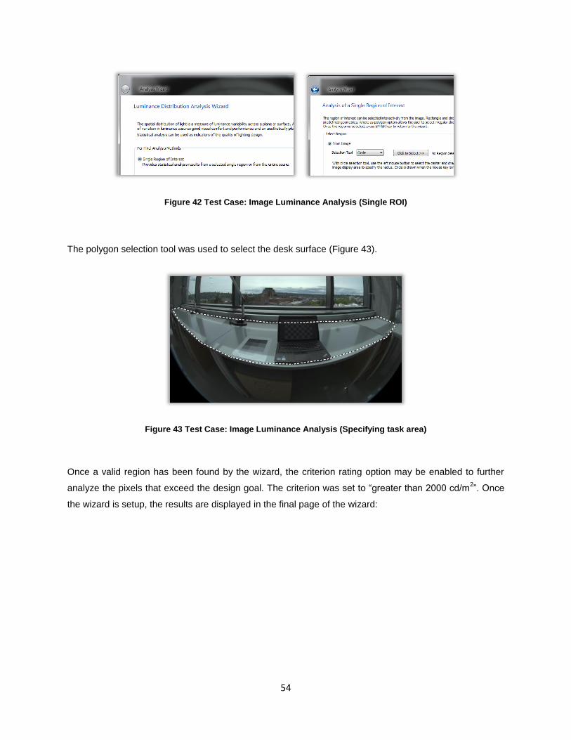
54
Figure 42 Test Case: Image Luminance Analysis (Single ROI)
The polygon selection tool was used to select the desk surface (Figure 43).
Figure 43 Test Case: Image Luminance Analysis (Specifying task area)
Once a valid region has been found by the wizard, the criterion rating option may be enabled to further
analyze the pixels that exceed the design goal. The criterion was set to “greater than 2000 cd/m2”. Once
the wizard is setup, the results are displayed in the final page of the wizard:

55
Figure 44 Test Case: Image Luminance Analysis (Results – no blinds control)
From the histogram and statistical data in Fig. 44, it is clear that more than 50% pixels of the selected
region are above the given criteria. The mean luminance value over the task surface is also over the
given criteria (2336 cd/m2).The above process of image post-processing, calibration and analysis were
repeated for the HDR image with the blinds rolled down. The results obtained were as follows:

56
Figure 45 Test Case: Image Luminance Analysis (Results – with blinds control)
With the blinds rolled down, the mean luminance drops down to 254 cd/m2 and there are no pixels greater
than the specified criteria. The example demonstrates that the blinds in the space were effective shading
devices at this particular date and time.
Luminance ratios between a task and immediate background can be analyzed using the “Multiple Region
Analysis” option in the analysis wizard. Two regions may be chosen – one with the computer screen as
the foreground and the other with the windows as the background.
Figure 46 Test Case: Image Contrast Analysis (Selecting foreground and background)

57
The polygon selection tool can be used to chosen to select the various regions. Once valid regions are
selected the next page in the wizard provides options to enable contrast calculations.
Figure 47 Test Case: Image Contrast Analysis (Statistics options)
The results for the contrast calculations are presented in the final page in the wizard. For this case study,
the following results were observed: The ratio of the mean luminance values between the task and the
window is calculated as 1:100.
Figure 48 Test Case: Image Ratio Analysis (Results - 1)

58
Figure 49 Test Case: Image Ratio Analysis (Results - 2)
For the contrast calculation, the foreground and background were chosen for the paper task on the target
(Figure 50). The contrast value for the task above was calculated to be 0.90.
Figure 50 Contrast calculation - Regions
As a final analysis, the glare analysis for the space is performed under both blind positions. The glare
analysis option from the analysis wizard was chosen from Tools > Analysis. No specific task area was
specified and all other Evalglare options were left to the default values.

59
Figure 51 Test Case: Image Glare Analysis (Options)
For the image with blinds not deployed, the DGP was calculated as 81% and for the image with blinds
rolled down completely the DGP was calculated as 42%. The Daylight Glare Probability of 81% means
that 81 people out of 100 would view that space as visually uncomfortable because of potential glare
sources. Figure 52 illustrates the images that were generated to identify the glare sources.
Figure 52 Test Case: Image Glare Analysis (Check files for the two cases of lighting control)

60
Conclusions
6.1 Summary
This primary purpose of the thesis was to develop a software for architects and lighting professionals that
provides a transition from the currently popular tools in their scripted format to a more user friendly and
interactive graphical user interface. Hdrscope offers several key advantages over current lighting analysis
tools. Not only is the software easy to use for novice users, it also provides several features such as
flexible region of interest selection, automated image capture for HDR, interactive wizards and an
integrated environment for lighting analysis. The aim of the software is to lower the entry barrier for
professionals and adopt lighting analysis in early design, development stages as well as post occupancy
analysis. The fundamental algorithms and programs running behind the scenes within hdrscope are
software functions derived from Radiance and Evalglare. Through wider adoption, the expectation is that
hdrscope would have a significant impact in enabling professionals to make informed decisions in terms
of visual comfort and performance of daylit and electric lit spaces.
The chapters in this thesis work are organized in a way so as to inform the reader about the theory
behind lighting simulations, the tools in use and detailed explanation of hdrscope. In Chapter 1, the
science behind lighting simulations was elaborated through an introduction to lighting simulations and
measurements techniques. Through a better understanding of the theory, the user can utilize software
programs efficiently.
Chapter 2 introduced various lighting simulation and analysis tools such as Radiance, Photosphere,
Evalglare and specialized software programs such as DIVA, Daysim, Matlab and etc. This chapter was an
introductory section to explain the current state of the art of lighting simulations and analysis tools, and
briefly discusses the advantages and drawbacks of these tools.
Chapter 3 introduces hdrscope – the main theme of this thesis work. This chapter may be considered as
a detailed user manual on the supported features of hdrscope, the commands issued for each feature
and the usage of various interactive tools.
Chapter 4 provides a step-by-step walkthrough of a sample case study. The case study was for post-
occupancy evaluation of daylighting performance of a laboratory space. Using hdrscope, the key lighting
metrics were calculated and using the available data from the various analysis tools in hdrscope, the
designer can evaluate the performance of the building and its occupants.
6.2 Key Contributions
Hdrscope has several features that are novel and it also provides user friendly options for existing
features in current lighting analysis tools. The following are some of the important contributions of the
software:
61
- Provides an integrated and user friendly GUI, thereby enabling professionals to adopt lighting
analysis without the need for learning commands and scripting. Hdrscope also obviates the need
for running several tools and data interchange.
- Incorporates interactive tools such as selection tools, analysis wizards and standard user
interfaces. Previously these were done through lengthy text based inputs which were
cumbersome.
- Provides a front end to several common Radiance picture processing and calibration features
- Automates several repetitive tasks such as camera image capture for HDR assembly (for Canon
Digital SLR cameras)
- Provides an easy way to visualize HDR images through Tonemapping and Falsecolor images.
6.3 Future Work
The following improvements to the software could further strengthen adoption:
- The software could benefit from more efficient and higher speed of operation. Currently Radiance
binaries are directly invoked as threads. By directly incorporating Radiance functions within the
code of hdrscope, there is scope for more optimization that would lead to faster performance.
- Support for more connected cameras such as Nikon, Point and shoot cameras, mirror-less
cameras and portable smartphone cameras would enable users to utilize any low cost camera for
HDR capture. Current support is for connected cameras that are normally used for professional or
research purposes and hence are expensive.
- Future work would also involve working on user feedback such as feature requests and bug fixes
that would ensure smoother operation of hdrscope.

62
References
[1] IES. (2011) The Lighting Handbook: Tenth Edition Reference and Application. New York: Illuminating
Engineering Society of North America.
[2] Ward, G. "The RADIANCE Lighting Simulation and Rendering System," Computer Graphics
(Proceedings of '94 SIGGRAPH conference), July 1994, pp. 459-72.
[3] Ward Larson, G and Shakespeare, R. (1997) Rendering with Radiance: The Art and Science of
Lighting Visualization. San Francisco: Morgan Kaufmann Publishers.
[4] Photosphere - Anyhere Software, http://www.anyhere.com/ Last retrieved 6 June, 2012
[5] Inanici M. “Application of the state-of-the-art Computer Simulation and Visualization in Architectural
Lighting Research," Proceedings of the 7th International Building Performance and Simulation
Association (IBPSA) 2001 Conference, Rio de Janeiro, Brazil, August 13-15, 2001.
[6] ISO 15469:2004(E)/CIE S 011/E:2003: Joint ISO/CIE Standard: Spatial Distribution of Daylight - CIE
Standard General Sky.
[7] Jensen, H. W. (2001). Realistic Image Synthesis Using Photon Mapping. In H. W. Jensen, Realistic
Image Synthesis Using Photon Mapping . Wellesley: A K Peters, Lts.
[8] Goral, C. M., Torrance, K. E., Greenberg, D. P., & Battaile, B. (1984). “Modeling the Interaction of Light
Between Diffuse Surfaces,” Computer Graphics, Vol. 18, No. 3.
[9] Pharr, M., & Humphreys, G. (2010). Physically Based Rendering: From Theory to Implementation. In
G. H. Matt Phar, Physically Based Rendering: From Theory to Implementation. Burlington: Morgan
Kaufmann.
[10] Reinhard, E., Ward, G., Pattanaik, S., & Debevec, P. (2005). High Dynamic Range Imaging:
Acquisition, Display and Image based Lighting. San Francisco: Morgan Kaufmann Publishers.
[11] Ward, G. (1991). “Real Pixels”. In J. Arvo, Graphics Gems II. Boston: Academic Press, Inc.
[12] R. Bogart, F. Kainz, and D. Hess, “OpenEXR image file format,” in ACM SIGGRAPH 2003, Sketches
& Applications, 2003.
[13] Inanici MN. “Evaluation of High Dynamic Range Photography as a Luminance Measurement
Technique”, Journal of Lighting Research and Technology, Vol. 38, no. 2, June 2006, pp. 123-136.
[14] Paul Debevec, Image-Based Lighting, IEEE Computer Graphics and Applications, v.22 n.2, March
2002, p.26-34,

63
[15] Tumblin, J., Rushmeier, H. E., "Tone Reproduction for Computer Generated Images.'' IEEE
Computer Graphics and Applications, Vol. 13, No. 6, November 1993, pp. 42--48.
[16] Ward, G. J., Rushmeier, H., and Piatko, C. “A visibility matching tone reproduction operator for high
dynamic range scenes,” IEEE Transactions on Visualization and Computer Graphics, Vol. 3 No. 4,
October-December 1997, pp. 291-306.
[17] Reinhard, E, Stark, M, Shirley, P, Ferwerda,J. “Photographic tone reproduction for digital images,”
ACM Transactions on Graphics (TOG), v.21 n.3, July 2002, pp. 267-276.
[18] US Department of Energy: http://apps1.eere.energy.gov/buildings/tools_directory, Last retrieved 6
June, 2012.
[19] HDRcapOSX: http://www.iesd.dmu.ac.uk/~jm/doku.php?id=resources:hdrcaposx. Last retrieved 6
June, 2012.
[20] Mathworks - Matlab: http://www.mathworks.com/products/matlab/. Last retrieved 6 June, 2012.
[21] Inanici MN. Transformations in Architectural Lighting Analysis: Virtual Lighting Laboratory.
Dissertation: The University of Michigan, College of Architecture and Urban Planning, 2004. Available
from: ProQuest Information and Learning, Ann Arbor , MI ; AAT 3121949.
[22] Inanici MN. “Per-pixel Data Acquisition with High Dynamic Range Photography” International
Commission on Illumination (CIE) 2005 Conference, Leon, Spain, 18-20 May, 2005.
[23] NREL: OpenStudio - Getting Started with Radiance: http://openstudio.nrel.gov/getting-started-
developer/getting-started-radiance. Last accessed 6 June, 2012.
[24] Autodesk Ecotect Analysis: http://usa.autodesk.com/ecotect-analysis/. Last accessed 6 June, 2012.
[25] DIVA for Rhino: http://diva4rhino.com/. Last accessed 6 June, 2012.
[26] Trimble Sketchup: http://sketchup.google.com/. Last accessed 6 June, 2012.
[27] DAYSIM: http://www.daysim.com/. Last accessed 6 June, 2012.
[28] Wienold, J. & Christoffersen, J. “Evaluation methods and development of a new glare prediction
model for daylight environments with the use of CCD cameras,” Energy and Buildings, Vol. 38 No. 7,
2006, pp.743–757. .
[29] Fraunhofer ISE - Evalglare by Wienold: http://www.ise.fraunhofer.de/radiance. Last accessed 6 June,
2012.

64
[30] Inanici MN and Navvab M. "The Virtual Lighting Laboratory: Per-pixel Luminance Data Analysis",
Luekos - Journal of the Illuminating Engineering Society of North America, Vol. 3 No. 2, October 2006,
pp. 80-104.
[31] Canon U.S.A: Support & Drivers: http://www.usa.canon.com/cusa/support. Last accessed 6 June,
2012.
[32] Inanici M. “Evaluation of High Dynamic Range Image-based Sky Models in Lighting Simulation,”
Luekos, Journal of the Illuminating Engineering Society (IES), 7(2), October 2010, 69-84.
[33] Matusik, W., Pfister, H., Brand, M., & Mcmillan, L. (2002). A Data-Driven Reflectance Model. ACM
Transactions on Graphics., pp. 22-23.
[34] Dolby Vision: http://www.dolby.com/professional/technology/home-theater/dolby-vision.html. Last
accessed 7 June, 2012.
[35] Texas Instruments DLP HDTV: http://www.dlp.com/hdtv/. Last accessed 7 June, 2012.
[36] Silicon Light Machines: http://www.siliconlight.com/. Last accessed 7 June, 2012.