Oxford Physics: Part C Major Option Astrophysics

High-Energy AstrophysicsGarret Cotter

garret@astro.ox.ac.uk

Office 756 DWB

Michaelmas 2011 Lecture 7

Today’s lecture: Accretion Discs Part I

• The Eddington luminosity and accretion rate.

• Accretion discs.

• Properties of the thin accretion disc.

• (Evidence for accretion onto black holes - will start if timepermits).

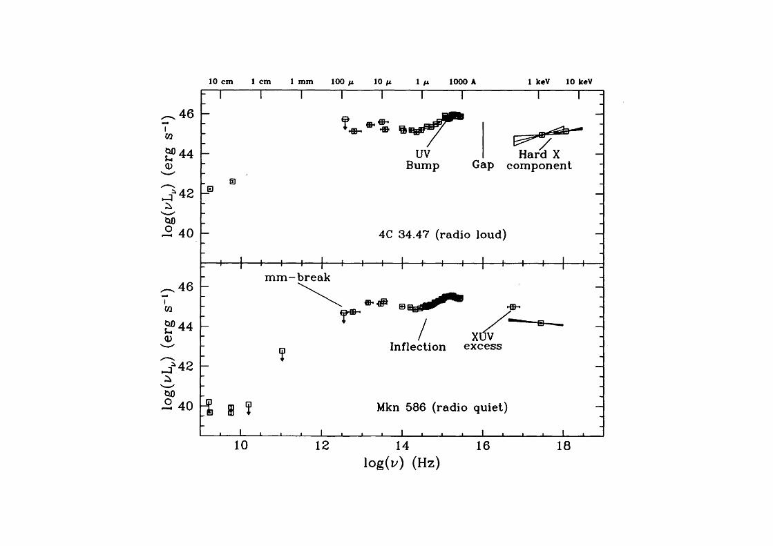
Average optical/UV spectra of quasars

Note non-blackbody spectrum with prominent emission lines.

The Eddington Luminosity

Today we will consider the accepted mechanism for the productionof the extreme luminosities of active galaxies: accretion of materialonto supermassive black holes. First we will consider theEddington accretion limit.

The Eddington luminosity was introduced in the context of massivestars. The notion is very simple: for any object in the depths ofspace, there is a maximum luminosity beyond which radiationpressure will overcome gravity, and material outside the object willbe forced away from it rather than falling inwards.

Sir Arthur Stanley Eddington (1882-1944)

Journalist: “Sir Arthur, it is said that onlythree people in the world understand rela-tivity!”

Eddington: “Yes I’ve heard that. I am tryingto work out who the third person is...”

The ingredients we need to derive the Eddington luminosity are:

• The mass of the central object, M

• The total luminosity, L

• A suitable opacity for radiation pressure against anysurrounding material. We will see that this must have thedimensions of area per unit mass.

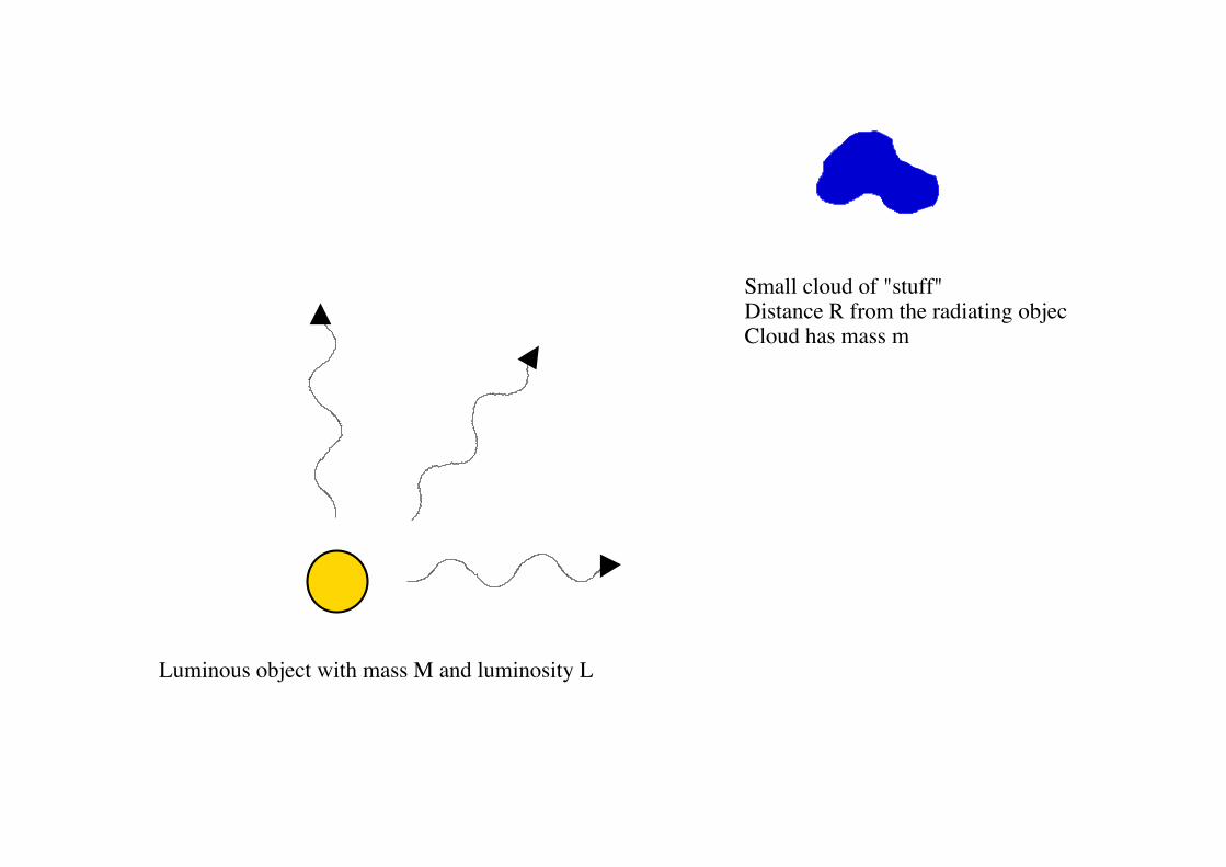
Small cloud of "stuff"Distance R from the radiating objectCloud has mass m

Luminous object with mass M and luminosity L

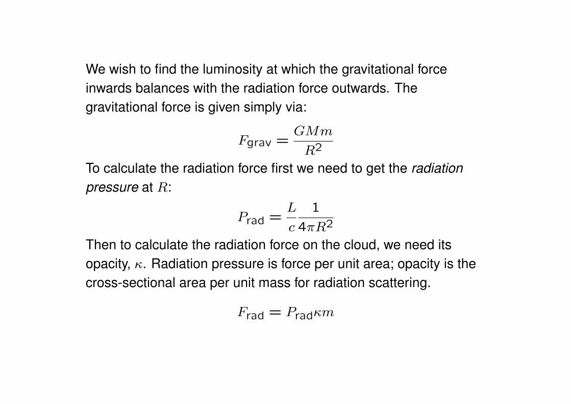
We wish to find the luminosity at which the gravitational forceinwards balances with the radiation force outwards. Thegravitational force is given simply via:

F

grav

=

GMm

R

2

To calculate the radiation force first we need to get the radiation

pressure at R:

P

rad

=

L

c

1

4⇡R

2

Then to calculate the radiation force on the cloud, we need itsopacity, . Radiation pressure is force per unit area; opacity is thecross-sectional area per unit mass for radiation scattering.

F

rad

= P

rad

m

Balancing the two forces gives:

GMm

R

2

=

Lm

4⇡R

2

c

And solving for this luminosity we get:

L =

4⇡GMc

Some important things to note here are:

• The Eddington luminosity depends only on the mass of theradiating object.

• We have assumed spherical symmetry.

Now, we have yet not specified a particular value for . Inhigh-energy accretion scenarios we make a useful approximationon the basis that the accreting material is mostly ionized hydrogenand the opacity is provided by Thomson scattering. Thecross-section will then come almost exclusively from radiationpressure on the electrons, but the mass lies almost exclusively inthe protons.

There will still be electrostatic forces between the e

�s and the p

+s;if we exert a radiation force on the cloud that is felt mostly by theelectrons, they will drag the protons along with them. Thus theapproximation is to set = �

T

/m

p

, and we get the followingapproximation for the Eddington luminosity:

L

Edd

=

4⇡GMcm

p

�

T

Note that this approximation for is not valid in all situations,especially in stars of all but the highest masses. E.g. in low massstars the opacity follows Kramer’s Law, / ⇢/T

3.5.

Eddington accretion limit

This becomes interesting when the luminosity of the central objectis derived from matter falling into it. In accretion onto compactobjects, infalling matter travels deep into the gravitational potentialwell of the central object. If it is possible to turn the GPE of theinfalling material into heat, huge luminosities can result.

First, however, let us consider the consequences for the limiting

rate at which such accretion can occur. Suppose a compact objectis accreting mass from its surroundings at a rate ˙

M . Next assumethat some fraction of the GPE can be radiated away. If we expressthis as a fraction ✏ of the rest-mass energy, then the luminosityradiated away becomes

L = ✏

˙

Mc

2

This has a profound implication. If our accreting object radiates atmore than the Eddington luminosity, even a glut of “fuel” will beblown away by radiation pressure: we get a natural feedbackprocess with a limiting accretion rate. We derive this by setting theaccretion luminosity equal to the Eddington luminosity:

✏

˙

Mc

2

=

4⇡GMcm

p

�

T

From which the limiting Eddington accretion rate is:

˙

M

Edd

=

4⇡GMm

p

✏c�

T

Accreting objects in practice

The rather unsubtle catch with this is that we have made noattempt to estimate ✏. In principle it could be as low as zero: if wesimply drop a brick radially into a black hole, it will disappear overthe event horizon taking all its energy with it.

However in a realistic astrophysical situation, accreting matter willhave angular momentum, forming an accretion disc. We will latercalculate the canonical value of ✏ which is used for black holeaccretion, and estimate the associated temperature and luminosityof the accreting material just before it disappears over the horizon.

First we will recap on the essential properties of black holes, thenconsider the conditions in the accretion disc.

Properties of black holes

In GR any point mass is described by the Schwarzschild (static) orKerr (rotating) metrics. We use the term black hole to describe anobject sufficiently compact (for its mass) that its event horizon hasnoticeable effects on spacetime and matter around the object. Fora point mass M , the Schwarzschild radius is

R

S

=

2GM

c

2

Note that this scales only with mass; RS

for a one-solar-massobject is 3 km. Formally this radius is called the event horizonbecause it is the furthest distance that a photon starting insideR

S

can reach; and once photons or matter from outside R

S

passbeyond it, they cannot escape.

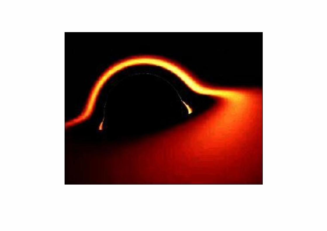
The event horizon is not a solid surface; matter falling inwardspasses straight through it. An external observer sees any lightemitted by the infalling object becoming infinitely redshifted as theobject passes over the horizon.

However, due to spacetime curvature near the horizon it is notpossible to have a stable circular orbit near the horizon. The last

stable orbit is at r = 3R

S

. For this part of the course we will takethis result as given.

Rotating black holes have a more complicated horizon and the laststable orbit is closer in. This may be very important for accretiononto real black holes.

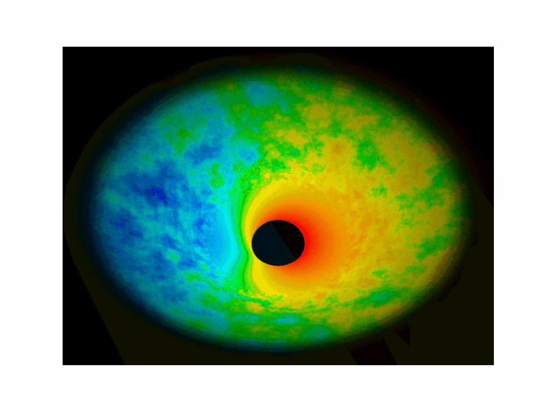
Accretion discs

The key to the extraction of energy by material falling into a blackhole is to remember that in real astrophysical situation is will havesignificant angular momentum. Gas falling onto a black hole in abinary star system will start with the tangential speed of the binaryorbit; gas falling onto the central black hole of an active galaxy maywell have an initial tangential velocity of hundreds of km s�1 if itbegins its descent from the outer regions of the galaxy. Abroad-brush picture is:

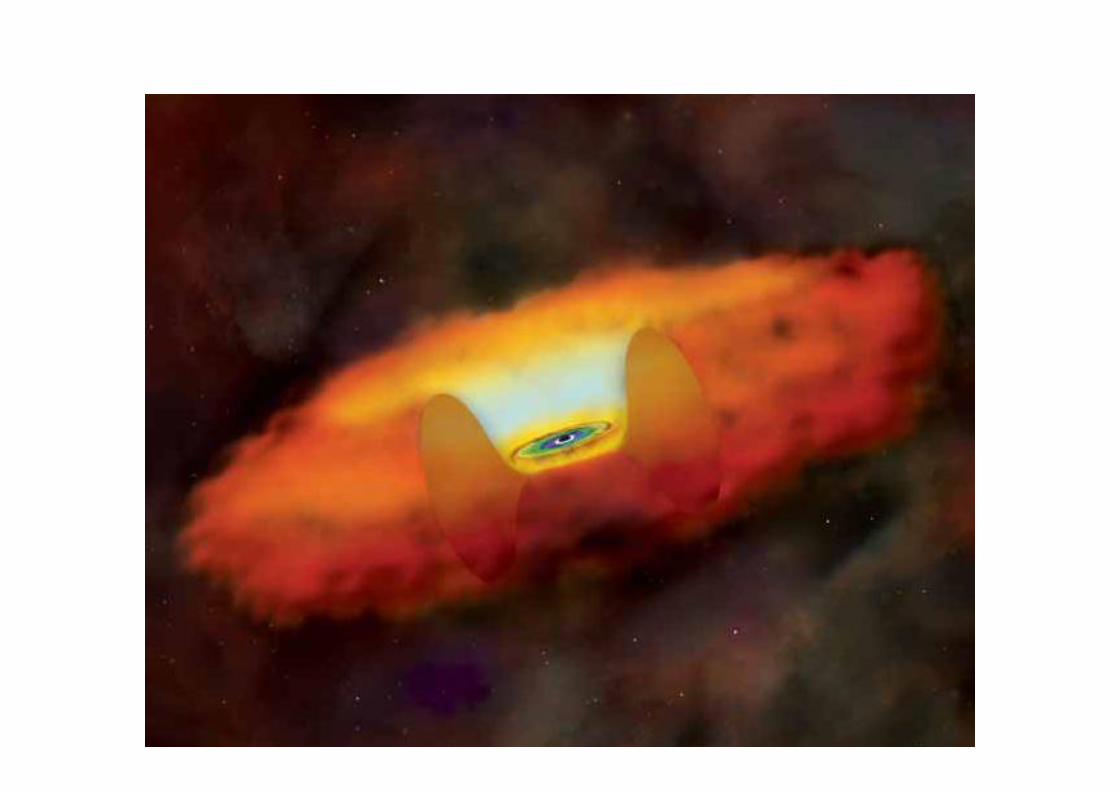
• An initially large cloud of gas extending well beyond the compact object will, if ithas net angular momentum, tend to flatten into a disc. This is because collisionsbetween particles in a direction parallel to the angular momentum L vector willtend to sum to zero, whereas collisions perpendicular to the L direction will tendto maintain the average circular velocity.

• As the disc becomes sufficiently dense, viscosity inside it both transfers

angular momentum outwards and heats the disc. This is how the GPE of theinfalling material is radiated away.

• In the most well-studied model, the disc is assumed to be physically thin andoptically thick. This allows the maximum amount of heat to radiate away from thesurface of the disk before matter falls into the black hole.

• Eventually we arrive at a reasonably stable state where matter spirals inthrough the disc, losing angular momentum via friction on its way in, becominghotter and hotter, until it falls off the inside edge (at the last stable orbit) andcrosses over the horizon.

Properties of the thin accretion disc

First of all, the disc must be in hydrostatic equilibrium. In the z directionperpendicular to the plane of the disc we must satisfy

dP

dz

= �⇢g

z

where g

z

is the vertical component of the gravitational acceleration due to thecentral object,

g

z

⇡GM

R

2

z

R

(using small-angle approximation). We can relate P and ⇢ via the sound speedin the gas, dP = c

2

s

d⇢, and then integrate to find that the density in the disc falls

off exponentially with height

⇢(z) = ⇢

0

exp

✓�

z

2

2h

2

◆

with a height scale factor given by h

2

= c

2

s

R

2

/GM .

Next we consider the speed of rotation. The particles in the discwill have orbits very close to Keplerian, so

v

2

rot

=

GM

R

.

The scale height can be re-written in terms of the rotational velocityvia

h

2

=

c

2

s

R

2

v

2

rot

so if we have R � h we must have v

rot

� c

2

s

and so the rotation

of the disc is highly supersonic. The same condition applies tokeep cold gas in the plane of the Milky Way with a rotationalvelocity of ⇡ 200 km s�1.

Viscosity in the disc

For the accreting material to fall into tighter orbits in the disc there must be anoutwards flow of angular momentum—a torque acting on the disc. Take the discviscosity to be ⌘ and consider a radius r in the disc with thickness t and angularvelocity !. The tangential force per unit area exerted by the disc inside r on thedisc outside r is given by

F = ⌘r

d!

dr

.

This force acts over an area 2⇡rt so the total torque between adjacent pieces ofthe disc is

� = 2⇡r

3

t⌘

d!

dr

.

Remember torque is rate of change of angular momentum!

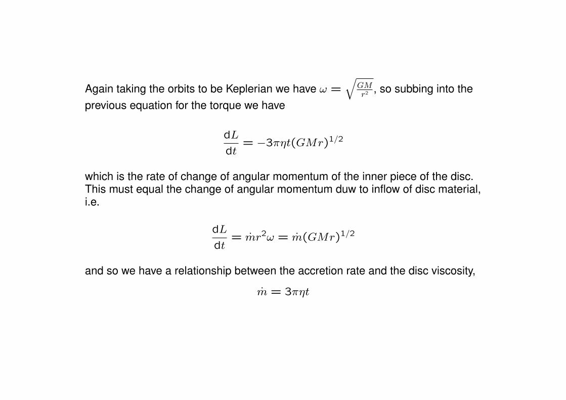
Again taking the orbits to be Keplerian we have ! =

qGM

r

2

, so subbing into theprevious equation for the torque we have

dL

dt

= �3⇡⌘t(GMr)

1/2

which is the rate of change of angular momentum of the inner piece of the disc.This must equal the change of angular momentum duw to inflow of disc material,i.e.

dL

dt

= mr

2

! = m(GMr)

1/2

and so we have a relationship between the accretion rate and the disc viscosity,

m = 3⇡⌘t

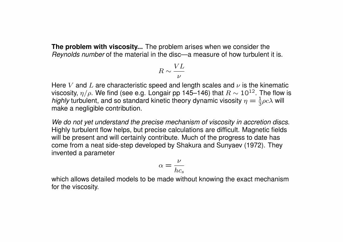
The problem with viscosity... The problem arises when we consider theReynolds number of the material in the disc—a measure of how turbulent it is.

R ⇠V L

⌫

Here V and L are characteristic speed and length scales and ⌫ is the kinematicviscosity, ⌘/⇢. We find (see e.g. Longair pp 145–146) that R ⇠ 10

12. The flow ishighly turbulent, and so standard kinetic theory dynamic visosity ⌘ =

1

3

⇢c� willmake a negligible contribution.

We do not yet understand the precise mechanism of viscosity in accretion discs.Highly turbulent flow helps, but precise calculations are difficult. Magnetic fieldswill be present and will certainly contribute. Much of the progress to date hascome from a neat side-step developed by Shakura and Sunyaev (1972). Theyinvented a parameter

↵ =

⌫

hc

s

which allows detailed models to be made without knowing the exact mechanismfor the viscosity.

Luminosity of a thin accretion disc

Neglecting the energy transport due to viscosity, we can calculate the rate atwhich accreting material in the disc must lose gravitational potential energy if it isto fall closer to the accreting object. For an annulus between r and r +dr, theenergy which must be dissipated will be

L(r) = �✓dE

dt

◆=

G

˙

MM

2r

2

dr

where ˙

M is the accretion rate and M is the mass of the central object. Includingviscous energy transport we gain a total luminosity three times this value(non-examinable—see Longair pp 149-150).

Temperature structure of a physically thin, optically thick disc

If the disc is optically thick, each annulus between r and r +dr will radiate as ablackbody with the luminosity derived above. Hence via Stefan’s Law(remembering the disc has two surfaces), the annulus at at r will radiate with2�T

4 ⇥ 2⇡rdr. Thus

�T

4

=

3G

˙

MM

8⇡r

3

and so

T (r) =

✓3G

˙

MM

8⇡r

3

�

◆1/4

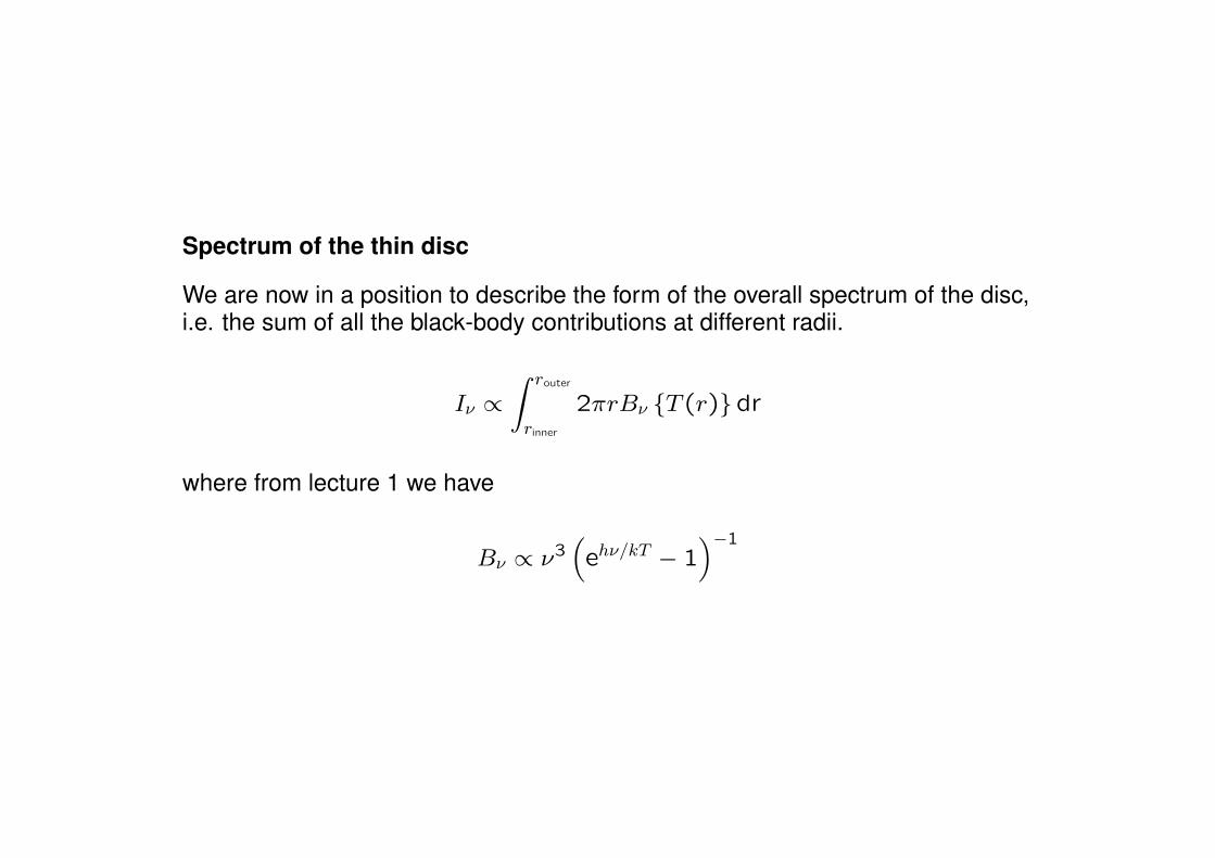
Spectrum of the thin disc

We are now in a position to describe the form of the overall spectrum of the disc,i.e. the sum of all the black-body contributions at different radii.

I

⌫

/Z

r

outer

r

inner

2⇡rB

⌫

{T (r)}dr

where from lecture 1 we have

B

⌫

/ ⌫

3

⇣e

h⌫/kT � 1

⌘�1

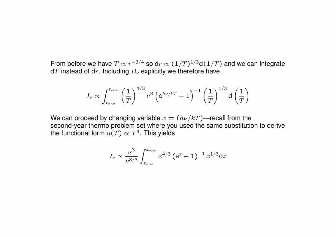
From before we have T / r

�3/4 so dr / (1/T )

1/3

d(1/T ) and we can integratedT instead of dr. Including B

⌫

explicitly we therefore have

I

⌫

/Z

r

outer

r

inner

✓1

T

◆4/3

⌫

3

⇣e

h⌫/kT � 1

⌘�1

✓1

T

◆1/3

d

✓1

T

◆

We can proceed by changing variable x = (h⌫/kT )—recall from thesecond-year thermo problem set where you used the same substitution to derivethe functional form u(T ) / T

4. This yields

I

⌫

/⌫

3

⌫

8/3

Zx

outer

x

inner

x

4/3

(

e

x � 1

)

�1

x

1/3

dx

The integral dx is just a numerical constant so we now have the shape of thespectrum over most of its range:

I

⌫

/ ⌫

1/3

.

Note, though, that the low- and high-frequency ends will have a different form:

• From the outer edge of the disc we will see the Rayleigh-Jeans tail ofT

outer

, I⌫

/ ⌫

2.

• From the inner edge, an exponential cut-off I⌫

/�e

�h⌫/kT

inner

�.

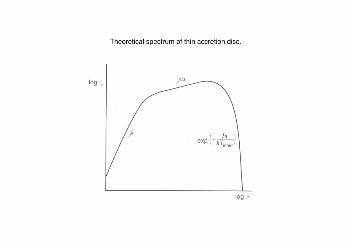
Theoretical spectrum of thin accretion disc.

1994ApJS...95....1E

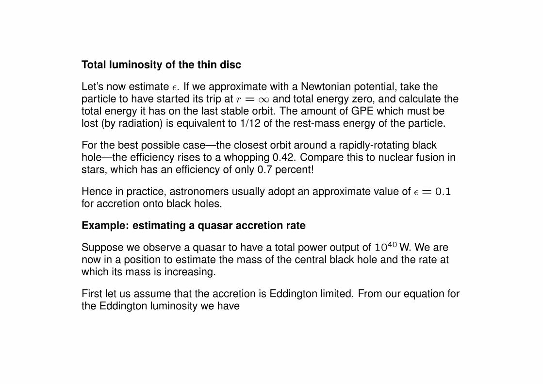
Total luminosity of the thin disc

Let’s now estimate ✏. If we approximate with a Newtonian potential, take theparticle to have started its trip at r = 1 and total energy zero, and calculate thetotal energy it has on the last stable orbit. The amount of GPE which must belost (by radiation) is equivalent to 1/12 of the rest-mass energy of the particle.

For the best possible case—the closest orbit around a rapidly-rotating blackhole—the efficiency rises to a whopping 0.42. Compare this to nuclear fusion instars, which has an efficiency of only 0.7 percent!

Hence in practice, astronomers usually adopt an approximate value of ✏ = 0.1

for accretion onto black holes.

Example: estimating a quasar accretion rate

Suppose we observe a quasar to have a total power output of 1040 W. We arenow in a position to estimate the mass of the central black hole and the rate atwhich its mass is increasing.

First let us assume that the accretion is Eddington limited. From our equation forthe Eddington luminosity we have

L

Edd

=

4⇡GMcm

p

�

T

from whichM = 7⇥ 10

8

M�.

And from our Eddington accretion rate, using ✏ = 0.1 we have

˙

M

Edd

=

4⇡GMm

p

✏c�

T

⇡ 3M�yr�1

Getting round the Eddington limit

The accretion may not always be Eddington-limited. It is, for example, possible toachieve ˙

M much greater than would be inferred by using the Eddingtonluminosity with ✏ = 0.1, by making the disc physically thick, and very low density,so that it is optically thin and matter doesn’t have time to radiate away so muchenergy before it falls over the horizon. This has the advantages of allowing blackholes to grow at a very high rate in the early Universe, and also of providing“funnels” which could be a mechanism for collimating outflows from accretingobjects.

Unfortunately simple analytical models of these discs are unstable, but theadvantages of thick discs are so great that much effort is put into modelling themnumerically... including the effects of strong magnetic fields.

It is also possible for an object to have a luminosity significantly greater than theEddington luminosity:

• In supernovae (somewhat trivially!)

• Where spherical symmetry is broken, with extremely collimated radiation ina direction different to the accretion direction

• Where accretion is not steady, e.g. bursts or radiation emitted whendiscrete clouds of matter fall onto a neutron star or white dwarf.

Evidence for black holes in AGNThere are several canonical pieces of evidence that supermassive black holesreally are there at the heart of AGN. Among these are:

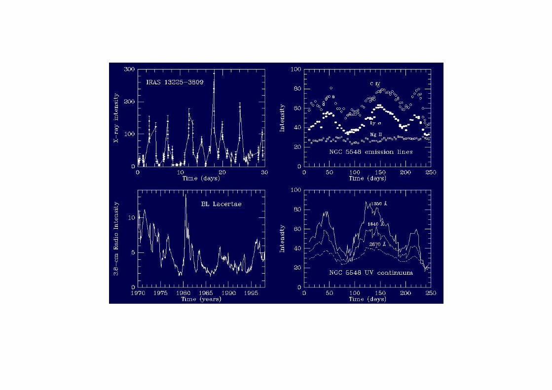
• Variability (in combination with Eddington luminosity).

• Stellar velocity dispersions.

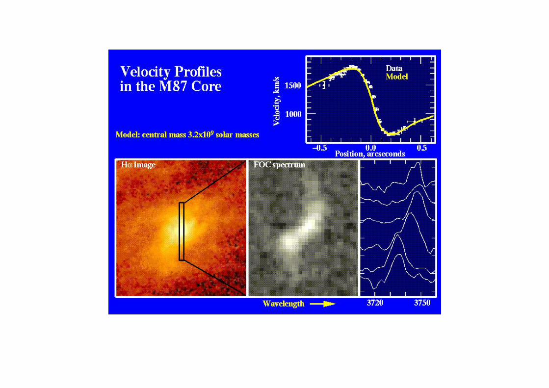
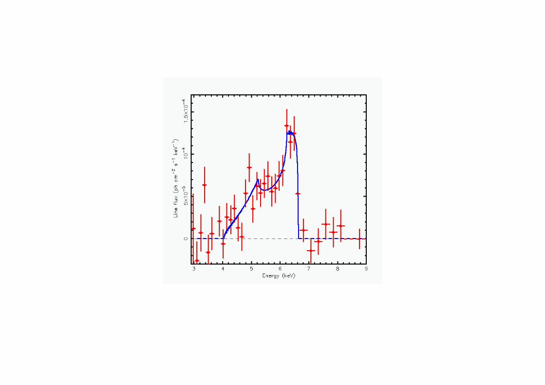
• Rotation speeds inferred from emission lines.

• The controversial history of X-ray line profiles.