1111~ ~1~~11~11 l~~el[ii~llll~t\f~l\\111 \1111~1\ ~1~11 , a 1160 003s22a a

Inelastic and Elastic Photoproduction of J/"1 (3097)

by

Bruce Hayes Denby

July 1983

High Energy Physics

FERMI THESIS LIBOFFCE

University of California, Santa Barbara

UNIVERSITY OF CALIFORNIA Santa Bal'bara

Inelastic and Elastic Photopl'oduction of J/~(3097>

A Dissertation submitted in partial satisTaction of the requirements for the degree OT

Doctor of Philosophy

in

Physics

by

Bruce Hayes Denby

Committee in charge:

Professor Rollin J. Morrison, Chairman

Professor Steven J. Yellin

Professor John L. Cardy

July 1983

The thesis of Bruce Hayes Denby is approved:

Cornmi'ttee Chairman /

July 1983

ii

ACKNOWLEDGEMENTS

I am extremely grateful to all members of the

collaboration for the many hours they have spent over

the past six or seven years building, debugging,

running, and analyzing results from the Fermilab

Tagged Photon Spectrometer Facility. I list them

here:

R. Morrison, M. Witherell, D. Summers, S. Yell in, v.

BharadwaJ, B. Denby, D. Caldwell, A. Lu, A. Eisner, R.

Kennett, U. Joshi

<University of California, Santa Barbara>

P. Estabrooks, J. Pinfold

<Carleton University, Ottawa, Canada>

S. Bhadra, A. Duncan, D. Bartlett, u. Nauenb erg, J.

Elliott

<University of Colorado, Boulder>

J. Appel, J. Biel, T. Nash, D. Bintinger, B. Schmidke,

L. Chen, C. Daum, M. Sokoloff, K. Stanfield, K. Sliwa,

M. Streetman, J. Bronstein, P. Mantsch, S. Willis

CFermi National Accelerator Laboratory>

M. Losty

<National Research Council of Canada> i i i

G. Kalbfleisch, M. Robertson

<University of Oklahoma, Norman>

J. Martin, G. Luste, G. Hartner, D. Gingrich, C. Zorn,

J. Spalding, K. Shahbazian, J. Stacey, 0. Blodgett, B.

Sheperd, 5. Bracker, R. Kumar

<University of Toronto, Toronto, Canada>

Of particular mention are the superhuman efforts put

forth by Tom Nash, John Martin, Steve Bracker, and

many others, during the early stages of getting E516

off the ground.

I give special thanks to my advisor, Prof.

Rollin Morrison,

offering guidance,

for his persistent efforts in

<which I appreciated more than I

always outwardly showed), and also for continuing to

support this research when it was unpopular with

others.

Prof. Mike Witherell has been particularly

helpful with the data analysis, and has been a

pleasure to work with.

I have profitted a great deal from numerous

conversations with Dr. 's Jeff Spalding, Jim Elliott,

Gerd Hartner. and Kris Sliwa. concerning physics and

data analysis.

iv

I thank Dr. 's David Bintinger and Penny

Estabrooks for their friendship and guidance while at

Fermi lab.

I thank Dr. Alan Duncan for allowing me to use

figures from his thesis, many of which are reproduced

here <41>.

I appreciate Dr. Ed Berger's taking the time to

discuss with me some of the theoretical questions

involved in this work.

I thank Dr. Vinod BharadwaJ and my fellow

graduate student <soon to be> Dr. Don Summers for

their friendship and moral support over the years. as

well as for valuable suggestions and advice.

The support from the Fermilab (former> Proton.

Physics. and Computing Departments has always been

first rate and is greatly appreciated.

My thanks and great respect go to Rudi Stuber.

Dave Hale. and all the UCSB shops for their excellent

performance during the construction of the SLIC and

outriggers.

I give heartfelt thanks to my mother for her

love. patience, and financial support during these

difficult years. I would like to dedicate this thesis

to the memory of my father.

taught me about perserverance. v

Harry H. Denby. who

Most important of all. I thank my wife, Carol,

without whose love, and understanding, I could not

possibly have succeeded in this endeavor.

vi

VITA

February 28, 1953--Born--Cleveland, Ohio.

1975--B.S., California Institute of Technology.

1975-1977--Research Intern, High Energy Physics,

Rutgers University.

1977-1983--Research Assistant, High Energy Physics,

Universit~ of California, Santa Barbara.

PUBLICATIONS

Equilibrium Charge States of Molecular Fragment

Hydrogen,

Bruce Denby and w. Whaling

Bul 1. Am. Phys. Soc. 2Q. ( 1975) 1500

Inclusive Cross Sections and Average Charged

Multiplicities in Inclusive KO and ~ Production in n-P L

Interactions at 147 GeV/c,

with P.E. Stamer et a 1. ,

Bul 1. Am. Phys. Soc. 22 (1977) 23

An Inexpensive Large Area Shower Detector with High

Spatial and Energy Resolution,

with V. K. BharadwaJ et al.,

Nucl. Inst. Meth. 155 (1978) 411

vi i

ABSTRACT

Inelastic and Elastic Photoproduction of J/~(3097>

by

Bruce Hayes Denby

The J/~(3097) photoproduction cross section on

hydrogen has been measured at a mean photon energy of

103 GeV, using the Tagged Photon

Spectrometer, Batavia,

Fermi lab

Illinois. The total cross

section, 21. 5 ± 2.4 nb <±257. normalization> has been

subdivided into 7 categories: 1> all events, 2)

forward elastic, 3) forward inelastic, 4> recoil

inelastic, 5) totally ela-stic, 6> inelastic, and 7)

inelastic with z = < . 9, as defined in the

text. The forward inelastic cross section observed in

this experiment is much smaller than that seen in

muoproduction experiments (16, 17), but is roughly

consistent with

predictions < 5).

second order perturbative GCD

The mean P+ of the forward inelastic

events is significantly larger than that of the

totally elastic events, in accord with the

muoproduction experiments as well as the second order

GCD predictions. vi i j

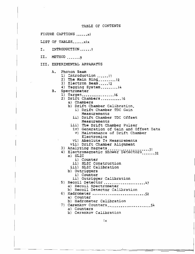
TABLE OF CONTENTS

FIGURE CAPTIONS .•••.• xi

LIST OF TABLES •....• xix

I. INTRODUCTION •••••• 1

II. t-A.ETHOD ....... 9

III. EXPERIMENTAL APPARATUS

A. Photon Beam 1) Introduction ...... 11 2 ) The Main Ring, ......... 12 3) Electron Beam ...•. 12 4) Tagging System ......... 14

B. Spectrometer l ) Target •..••••••........ 16 2) Drift Chambers ..•••••••.. 16

a} Chambers b) Drift Chamber Calibration.

i) Drift Chamber TDC Gain Measurements

ii) Drift Chamber TDC Off set Measurements

iii) The Drift Chamber Pulser iv) Generation of Gain and Offset Data v) Maintenance of Drift Chamber

Electronics vi) Absolute T$ Measurements

vii} Drift Chamber Alignment 3) Analyzing Magnets .•......•••.•.•.•..••. 31 4) Electromagnetic Shower Detectors ..••... 32

a) SLIC i) Counter

ii) SLIC Construction iii) SLIC Calibration

b} Outriggers i) Counter

ii) Outrigger Calibration 5) Recoil Detector ...................... 47

a) Recoil Spectrometer b) Recoil Detector Calibration

6) tiadrometer ............................ 52 a) Counter b) Hadrometer Calibration

7) Cerenkov Counters ......•••..•.......•... 54 a) Counters bl Cerenkov Calibration

ix

8) Muon Wall ..•...•.•••.••.•••..•••• 56 a) Muon Counters b} Muon Wall Calibration

c. Triggers 1) Tag-H ....••.••.•..•••••.••. 57 2) Recoil Triggers •••••••••••••• 58 3) Dimuon Trigger •••••••••••••• , •••• 60

D. Data Acquisition Sys tern •••••.•••••••••• 62

IV. DATA ANALYSIS

A. Producing the 1/J Signal •••••••••••••••••. 64 B. Definition of Elastic and Inelastic, .••••• 70 c. Classification of Events •••••••• 73

1) Forward Classification 2) Recoil Classification

D. Determination of Z •••• , .•.•.••.•••.• 80 E. Uncertainties in Classification, •.•••.•••••.. 85

1) Uncertainties in Forward Classification 2) Uncertainties in Recoil Classification

V. EFFICIENCY CALCULATIONS

A. Track Reconstruction Efficiency .•••• 90 B. Elastic Monte Carlo ..•••••.••••••••••••••• 92 c. Inelastic Monte Carlo •••••.•••••••••.•• : •••••• 94

VI. RESULTS, •••••••••• ,. 97

VII. DISCUSSION OF RESULTS . , ••••• , 105

APPENDIX A: Figures .••••••••• 111

APPENDIX B: Tables .••.•••••.••.•••• 166

LIST OF REFERENCES .•••••••• 173

x

FIGURE CAPTIONS

1> First order GCD Psi photoproduction diagram:

Photon Gluon Fusion.

2) Second order GCD Psi photoproduction diagrams

Cref. 3, 5).

3> Aerial view of Fermi National Accelerator

Laboratory CFermilab>, Batavia, Illinois.

4> Schematic of Fermilab beam lines.

5> Proton Area beamlines.

6) Pre-target beamline components, target b-ox,

and electron transport system. Components

labelled "BH" or "BV" are horizontal and vertical

bending magnets, respectively. "GH" and "GV"

components are horizontal and vertical quadrupole

(focussing> magnets. "CH" and "CV" components

are collimators. Components labelled "SC" are

SWICS, which are small wire chambers used for

monitoring beam profiles. TEBY is the primary

target, and CONVET is the converter.

7> Electron and tagged photon beam components.

Components labelled "LT" are lead targets,

xi

which

can be placed in the beam in conJunction with the

SWICS to make the electron and photon beams more

visible. AN440C is the tagging magnet, and ERAO

is the radiator.

8) Electron beam focussing components and beam

profiles.

9) Electron yield per 400 GeV pToton versus

electron energy.

10) Schematic layout of tagging system. L1-L13

are the tagging lead-glass blocks. H1-Hl3 are

the hodoscopes. Counters labelled "A" are used

in anti-coincidence.

dump counters.

D1 and D2 are electron beam

11> Typical tagged photon energy spectrum.

12) Layout of the drift chambers showing z

coordinates.

13) Drift chamber cell configuration.

14> Drift chamber amplifier discriminator card

with LeCroy OC201's, showing loop antenna from

drift chamber pulser.

xii

15> Cutaway view of drift chamber inductive pulse

sp 1 i tter. Only 2 of the 36 or 49 outputs are

shown.

16> Printed circuit board artwork used in making

the inductive pulse splitters.

17> The inductive/capacitive coupler used to feed

pulses into the high-voltage planes of the drift

chambers for timing offset measurements.

18> Circuit diagram of the drift chamber test

pulser, used for measuring gains and offsets of

the TDC 's.

19> The SLIC electromagnetic shower counter.

20> Illustrating the construction of the SLIC.

Shown are the three orientations of the

corrugations and their arrangement in the tank.

21> Implementation of the wavebar readout system.

The U view, which read out on top of the SLIC, is

shoum.

22> In a), the intersection of an electron shower

with a typical

illustrating the

SLIC counter is sh own,

pair calibration technique xi i i

described in the text. In b), an actual shower

shape curve from the ~alibration program is

shown, with a fitted Gaussian <asterisks>.

23) Schematic overview of the Tagged Photon

Spectrometer Facility. Counters are described in

detail in the text.

24) The Tagged Photon Spectrometer Facility,

Fermi lab.

25> OUTRIGGER electromagnetic shower counter,

showing X and Y readout schemes.

26> Photon's-eye-view of the Recoil Spectrometer.

27> Cutaway view of recoil PWC's.

28> Cross section or a recoil PWC.

29> The Hadrometer.

30> Upstream Cerenkov counter <Cl>.

31> Downstream Cerenkov counter CC2>.

32> Cerenkov counter optics.

33> Cerenkov counter mirror segmentation (both

counters have the same seg~entation arrangement), xiv

and mirror suspension system.

34> Schematic of the Muon Wall.

35) Logic diagram of the Hadronic trigger

C tag-H>.

36) Layout of

showing location

counters.

the

of

dimuon trigger

the Pre-C and

37> Dimuon trigger logic diagram.

38> Data acquisition system.

counters,

Caboose

39) x, y, and Z position of dimuon vertices for

the final data sample. Also shown is the

distribution in distance of closest approach.

These distributions are quite clean and do not

reduce the significance of the signal.

40> Final dimuon mass spectrum showing all events

above 1. 5 GeV/c2. There are 147 events in the

range 2.8 ~MCµ+µ->< 3.4 GeV/c2.

41) The final dielectron mass spectrum. There

are 63 events in the range 2.8 ~MCµ+µ->< 3.4

GeV/c2.

·xv

42> Dimuon events which were classified as

forward elastic <defined in text>.

events between 2.8 and 3.4 GeV/c2.

There are 110

43> Dimuon events which were classified as

forward inelastic Cdefined in text>.

37 events between 2.8 and 3.4 GeV/c2.

44 > In a> we plot z =

There are

wh el' e

Ex<1> is the total energy of all detected non-Psi

particles; i.e., assuming that al_l forward energy

is detected. In b) we plot z = E\jJ /CE\jJ +F*Ex Cl>); i.e., we correct z for the

measured mean inelastic energy deficit.

45> We use the means of these distributions to

calculate the average fraction of non-Psi forward

energy that we detect. In a>, R = for

elastic forward events, which peaks near 1, as it

should. In b), R = E\jJ /Ey for inelastic forward

events; this distribution peaks below 1 since the

other particles carry some energy. In c >, R = +Ex < 1 > > /E y ;

inelastic energy.

those of a> and b>.

we add back in the detected

The peak is midway between

xvi

46) Plotted are the numbers of charged tracks,

photons, pi-zeroes, hadronic neutrals detected

per inelastic forward event. In e> the total

number of particles is shown;

count as two particles.

here, pi-zeroes

47) Total forward mass for those inelastic events

with two extra tracks of opposite charge and no

extra photons or hadronic neutrals. The Psi

four-vector has been constrained so that its

s~uare is exactly the Psi mass. There is a peak

of 4 events near the Psi-prime mass 3.685.

48> The overall event reconstruction efficiency E

for elastic events as a function of photon energy

k.

49) Mean P+ versus z from the inelastic

monte-carlo <histogram>. The smooth curve is

from the color singlet model of Berger and Jones

< ref. 5 > . Bo th are e v a 1 u ate d at l 00 Ge V.

50) Overall inelastic event reconstruction

efficiency E from the inelastic monte-carlo as a

function of z, evaluated in two bins of P+· The

photon energy is 95 Gev.

xvii

---- -· ---------- -------------------

51> Overall inelastic event reconstruction

efficiency E as a function of z, evaluated for

two photon energies. All P+ values are included.

52> Number of events corrected for efficiency

plotted versus the corrected z value <defined in

text> for that event. The recoil inelastic

events, which are de~ined to be in the highest

bin are left off in this plot. Also shown is an

estimate of the contribution from ~, based on the

measurement of ref. 15.

53) The same distribution as in figure 52 but the

recoil inelastic events are added into the

highest bin.

54) a> shows the P+ distribution for totally

elastic (defined in text> events. b) shows the

P+ distribution for TDrward inelastic (defined in

text> events. The inelastics clearly have a

flatter P+ distribution.

xviii

LIST OF TABLES

I. Drift Chamber Resoultions and Efficiencies ... l67

II. Cerenkov Counters ...... 168

III. Cerenkov Cells ...... 168

IV. Raw and Corrected Even ts in Each Category .... 169

V. Fractions in Each Category ...... 170

VI. A. Cross Sections in Each Category ...... 171

B. iJ.i'-Subtracted Cross Sections in Each Categ .. 171

VII. A. Comparison of Elastic Cross Sections ...... 172

B. Comparison of Inelastic Cross Sections ...... 172

C. Comparison of Inelastic Ratios ...... 172

xix

1

I. INTRODUCTION

Production of the J/1pC3097> meson is a

particularly attractive vehicle for an experimental

study of the strong interaction because the J/1p has

large branching fractions into dimuons and dielectrons

< 7.4 percent into each), which provide very clean

signatures for events containing the J/41.

Photoproduction is likely to be one of the best

methods of producing the J/'41 because: 1> Vector Meson

Dominance <1> dictates a sizable coupling of photons

to vector mesons, Cthe J/'41 is a vector meson like the

and q», and 2> There are fewer hadronic

background processes in photoproduction.

From a th eoret i ca 1 standpoint, the J/41 has proved

an excellent system in which to study the strong

interaction via perturbative Guantum Chromodynamics

CGCD>. The J/41 has been successfully interpreted as

one of a family of bound states, ca 11 ed c harmon ia, of

a charmed ( c) and anticharmed Cc> quark (2).

Perturbative GCD should be valid when the running

coupling constant a 5 cm2), is smal i, which in turn

requires that the mass scale, m2, of the process under

consideration be large. In the case of the J/1p, the

2

large charmed quark mass, me = 1. 5 GeV/c2 ~ . 5M 1./1 '

ensures that « 5

taken to have

w i 11 b e s ma 1 1 < 3, 4, 5 >.

a value of 0.2 to

It is usually

0.4 (4,5>.

Photoproduction of the J/~ should perhaps be simpler

to calculate than hadropraduction since: 1> The photon

has a direct, pointlike coupling to the cc system, and

2> There are no comp~ting Drell-Yan Cquark-antiquark

annihilation> diagrams to lowest order in a 5 <7>.

The simplest GCD diagram that can be drawn for

JI~ photoproduction, shown in figure 1, involves the

photon's materialization into a cc pair, with one of

the quarks then interacting with a gluon -rrom the

target nuc 1 eon. This has come to be referred to as

Photon Gluon Fusion, or simply 1GF. Gualitatively,

this diagram is expected to describe the elastic part

of the J/~ photoproduction cross section c4,9, 10>. In

the framework of the parton model, gluons are taken to

be on-shell ca, 101 11). Thus for a one-gluon exchange,

-t = G2 ':! Q, indicating forward, diffractive

scattering where the J/~ has very low P+· Thus far,

the first-order 1GF diagram describes all cc

production, both bound and unbound. It has become

common to assume, on the basis of semi-1oca1 d ua 1 i ty

arguments, that the kinematics of the real final state

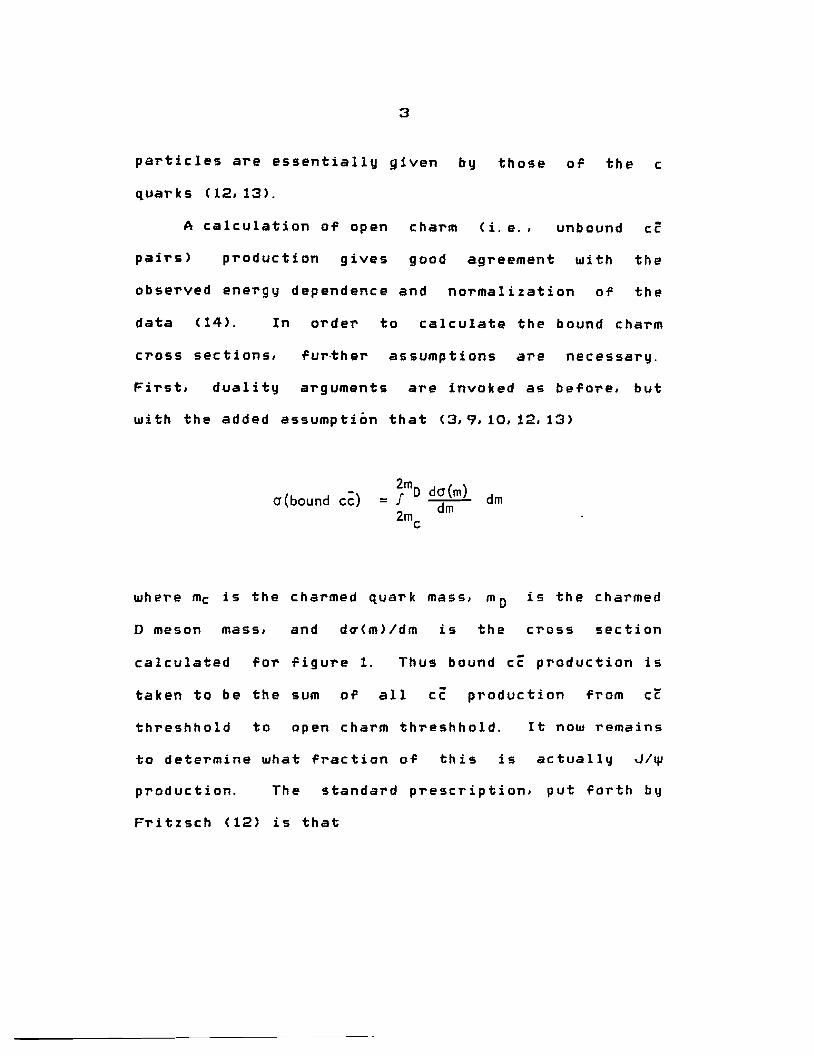
3

particles are essentially given by those or the c

quarks ( 12, 13).

A calculation of open charm < i. e. ' unbound cc

pairs> pT'oduction gives good a.greement with the

observed energy dependence and noT"malization of the

data C 14>. In OT'deT' to calculate the bound charm

cross sections, further assumptions are necessary.

First, duality aT"guments are invoked as before, but

with the added assumption that c3,9, 10, 12, 13>

O' (bound cc) dm

where me is the charmed quark mass, m0 is the charmed

D meson mass, and dq(m)/dm is the cross section

calculated fol' figure 1. Thus bound cc production is

taken to be the sum of all cc production from cc

thT"eshhold to open charm threshhold. It now remains

to determine what fraction of this is actually JI~

production. The standard prescription, put forth by

Fritzsch <12> is that

4

= F • cr (bound cc)

where F is the reciprocal of the number of charmonium

states, usually taken to be in the neighborhood of 8.

This prescription is somewhat arbitrary, and probably

wrong, since it predicts equal contributions from all

charmonia; recent photoproduction data (15) have shown

that the tp' cross section is only about 207. of the J/ip

cross section. Nevertheless, F must have some value

less than one, and using this method, it is possible

to reproduce the energy dependence of existing elastic

Jlip photoproduction data rather well <see, e.g. ref.

9>.

The use of fig. 1 has a number of fundamental

shortcomings: 1> Since only one gluon interacts with

the cc system, color cannot be conserved, and

furthermore, the cc system cannot be in a Jpc. = 1-­

state. Additional soft gluon<s> must be emitted in a

way which is not specified by the theory. and which is

assumed not to affect the kinematics of the charmed

quarks ( 12). 2> It is necessary to invoke duality

arguments to calculate cross sections. 3> The F

factor makes the normalization uncertain. 4) It

5

probably describes only the elastic cross section.

The lowest order color-conserving diagrams are

shown in figure 2 (3,5>. These two-gluon diagrams are

of order a~ and can qualitatively be thought of as

describing inelastic JI~ photoproduction, since the

JI~ now carries only a fraction z = E~ /Ey of the

energy of the photon, the rest being carried by a

g 1 uon. Al so, s i z eab 1 e P+ can now be transmitted to

the JI~ <10, 14>. In calculating with these diagrams,

one can again invoke duality and an F factor (3) to

get cross sections. The inelastic cross sections are

thus expected to be of order a 5 times the - elastic

cross sections < 4, 6, 9 > , i. e. , about 30 p er c en t of th e

elastic cross sections.

An alternative approach has been adopted by E.

Berger and D. Jones ( 5). Here an explicitly

normalized Ci. e., parameter free> cross section is

calculated by representing the cc pair as a normalized

JP = 1- JI~ wavefunc ti on. The coup 1 i ng strength of

the JI~ to cc is specified by the electronic width of

the J/~, I'ee = 4. 8 keV. Berger and Jones stress

that the use of the parton model is Justified only in

certain kinematic regions. in particular.

6

1. 2 GeV/c2 where mx is the mass of X in

This excludes elastic production,

and quasi-elastic production

2. I t I

They show that these conditions will be satisfied only

when

z < .9 "'

In our analysis, we shall often make use of this cut,

both to allow comparison with theoretical predictions,

and to allow our data to be compared to other data,

which are often cut in this way.

The main -Features of inelastic J/tp

photoproduction in the Berger and Jones model are: 1)

A z distribution peaked at high z, falling off rapidly

at low z. 2) High P+· The predicted mean P+ at Ey =

100 GeV is about 1 GeV. 3> A relatively low cross

section. At 105 Gev, the predicted inelastic cross

section for z < .9 is 2.9 nanobarns. The measured

elastic cross section at this energy is roughly 12 to

7

20 nanobarns This prediction is in

keeping with the qualitative notion that the inelastic

cross section should be of order a5

elastic.

Since the Berger-"-'ones model

normalized cross section. it can be

data. Inelastic Jlcp data exists

muoproduction experiments,

times the

predicts a

compared with

from two

the

Berkeley-Fermi lab-Princeton group <BFP, 17,19;2u, and

the European Muon Collaboration <EMC, 16, 20, 29>. The

data from these two experiments, which both used

spacelike virtual photons on iron targets. have been

corrected for nuclear effects, and extrapolated to GZ

= 0 to yield numbers for photoproduction on single

nucleons. While both experiments report z

distributions in rough agreement with Berger and

Jones, the experimental inelastic cross sections are

roughly a factor of 5 larger than the predictions

(5, 161 17, 20. 21. 29). As the only adJustable parameter

in the Berger-Jones model is the value of «s• which

probably cannot vary by more than about 50 ;., there is

little chance of reconciling this theory with this

data C43>.

The inelastic data thus seem to be at serious

8

odds to the theoretical predictions of second order

perturbative GCD. In what follows, we will show that

a very different result is obtained when the J/~ is

photoproduced on hydrogen with real (Q2 = O> photons.

9

II. METHOD

Requisite to the photoproduction of IJI on

hydrogen, and the subse~uent analysis of events are:

1. A high energy photon beam with sufficient

luminosity · to produce a statistically strong

sample of ~ events in a reasonble length of

time.

2. A hydrogen target.

3. A multipaT'ticle spectT'ometeT' with the

capability to detect and measure four-vectors

of all charged and neutral particles produced

in the hadronic interaction of the photon

with the proton in the target.

4. An experimental trigger with the ablility to

select the desired events out of a huge

backgT'ound of electromagnetic processes, as

well as reJect other. less interesting

hadronic pT'ocesses.

10

5. A data acquisition system which has the

ability to record data from over a thousand

different channels on each event, at a rate

of about 100 events per second.

6. Off line reconstruction software, and

computing p~wer, which can reduce millions of

raw triggers down to a manageable set of

reconstructed data summary tapes on a

reasonable time scale.

In the following section, each of these components, as

implemented

in detail.

in Fermilab experiment E516, is discussed

1 1

III. EXPERIMENTAL APPARAT~S

A. THE PHOTON ~

1. INTRODUCTION

To photoproduce a ~ meson on hydrogen. a photon

energy of about 8 GeV or more is necessary, however.

earlier experiments <22-25, 18) have shown that the

cross section for ~p~~p at photon energies near 100

GeV is roughly 50 times larger than at 11 GeV. and

thus, it is advantageous to make use of photons of the

highest available energies in order to ensure a high

production rate.

beam be free

It is also important that the photon

of hadronic contamination since

hadroproduction cross sections are typically two

orders of magnitude larger than the total

photoproduction cross section. Finally. it is useful

to know the energy of each photon in the beam with

good precision so that energy balance constraints can

be imposed, and as will be seen for this experiment,

for use in triggering.

The tagged photon beamline of the Tagged Photon

Specrometer at Fermi National Accelerator Laboratory,

Batavia. Illinois, provides a very clean beam of high

energy photons of known energy. The photons are

12

produced in a multi-step process which is outlined

below.

2. THE MAIN RING

All the particle beams for high energy physics

research at Fermilab have as their source the large

main ring. a proton synchrotron. Protons from a

hydrogen ion source are accelerated to 750 keV in the

Cockcroft-Walton, to 200 MeV in the LINAC, and to 8

GeV in the booster ring before entering the 4 mile

circumference of the main ring where they are

accelerated to 400 GeV. <The peak energy is currently

b e i n g u p grad e d t o 1000 Ge V. >

The protons are resonance extracted from the main

ring and directed onto the septum. This is a set of

wire planes at high positive electrostatic potential

set parallel to the beam direction. The protons are

repelled from the wire planes as they pass them and

the beam is thereby split into three beams, which

enter the swithchyard where they are focussed and bent

magnetically toward the three main experimental areas,

Meson, Neutrino. and Proton. See figures 3, 4, 5 for

a layout of the main ring and experimental areas.

3. ELECTRON BEAM

13

The proton area beam is split in enclosure H by

another septum into three beams which go to the PWest,

PCenter, and PEast areas. In enclosure El in the

PEast beamline the protons can be directed either onto

the Wide-Band or Tagged Photon primary targets.

Protons hitting the 30 cm. long beryllium target

<TEBY> of the Tagged Photon beamline produce charged

and neutral secondaries. The charged secondaries are

swept magnetically into a beam dump,

neutra 1 s, consisting of neutrons, KO, L

while the

and photons

Cfrom wO) pass forward to a .32 cm thick C. 5 radiation

length> lead converter located 12 meters downstream.

Roughly 407. of the photons form e+e- pairs in the

radiator, while less than 27. of the hadronic neutrals

interact to form more secondaries. The converter is

followed by an electron beam transport system

consisting of two stages, each with bending and

focussing magnets and collimators. The undeflected

neutrals pass into the neutral dump, as do any

positively charged secondaries. By adjusting the

magnet currents, the beamline can be tuned ta

transport a beam of 10 to 300 GeV/c. The momentum

resolution of the beam is about ± 2. 57.. The momentum

selection reduces the already small hadronic

14

contamination of the electron beam to a negligeable

level. The beamline components are shown in figures

The electron beam intensity per incident

400 GeV proton is shown in figure 9 as a function of

electron beam energy.

4. TAGGING SYSTEM

The tuned electron beam now enters the tagging

system. Electrons pass through a copper radiator, and

in so doing create bremsstrahlung photons with an

energy spectrum given by the thin radiator

approximation C34>:

N (k) dkdx = ~(!!_ - ~(~ ) + k 3 3 E

0

where N< k > is the number or photons near energy k, d x

is the thickness in radiation lengths, and E0 is the

electron beam energy. A simple dk/k spectrum is often

used in rough calculations. The photon angles are

dominated by the multiple scattering angle of the

electron in the radiator, which for all practical

purposes is e = 0. While the photons pass straight

forward into the experimental hall, the electrons are

15

bent by the tagging magnets toward the tagging blocks.

This is a set of 13 lead glass or lead-lucite blocks

instrumented with phototubes and used as shower

counters to measure the energy of the electron after

radiating. E'. The energy of the tagged photon is

then simply

E = E - E1

y 0

A set of hodoscopes, H1-H13, in front of the lead

glass counters gives an independent measurement of the

position of the electron.

pictured in figure 10.

The tagging system is

To enhance the photon T 1 U XI one wants the

radiator as thick as possible. but as the radiator

thickness increases.

photon wi 11 pair

increases. as does

the probability that the radiated

produce in the radiator also

the probability of multiple

bremsstrahlung. The thickness .2 radiation lengths

was chosen to give as high a rate as possible while

keeping the pair production and multiple

bremsstrahlung at an acceptable level.

Additional bremsstrahlung photons from a single

16

electron pass into the C-counter, a total absorption

shower counter located downstream. The tagging energy

in this case is corrected by

Ey = E - E' - E 0 c

where Ee is the energy of the additional photon<s> in

the C-counter. The fact that the radiator is no

longer thin causes the spectrum to deviate somewhat

from the thin radiator approximation given above. In

particular the high energy end of the spectrum does

not scale linearly with radiator thickness. The

resulting tagged photon energy spectrum for this

experiment is shown in figure 11.

B. SPECTROMETER ii5U.

1. TARGET

The target consists of a 1. 5 meter long, 1 inch

radius flask of .005 inch mylar, filled with liquid

hydrogen . This was surrounded by a 2. 5 inch radius,

. 5 inch thick foam vacuum Jacket covered with another

layer of mylar.

2. DRIFT CHAMBERS

17

a. CHAMBERS

Four chambers, herein referred to as 01, 02, D3,

and D4, were used to determine traJectories and

charged particles in the forward momenta o.P

spectrometer. The overall layout of the chambers is

shown in figure 12. Space points are derived from the

coordinates of tracks in wire planes of three

orientations, namely U and V planes, at ± 20. 5 degrees

to vertical, and X planes, which are vertical. The

presence of three views allows most ambiguities in

track positions to be resolved.

Dl, the small chamber located inside Ml, consists

of two assemblies, each containing u, V, X, and X'

planes. The X' plane is simply another partial X

plane, offset slightly from the X plane, for added

redundancy near the beam where rates are highest. D2

and 03 each have three UXV assemblies. and D4 has a

single UXV assembly. Thus the traJectory of a

particle traversing all four chambers will have a

total of 9 measurement points on it: 2 in DL 3 each

in D2 and 03, and one in D4.

In 01-03, sense wires are at ground, and high

voltage wires are at negative potential. In 04, sense

18

wires are at positive high voltage, the field wires

are at ground, and the field wires in the sense plane

can be set at a small positive or negative voltage.

The drift cell configuration of the chambers is shown

in figure 13.

All chambers were mounted on rails so that they

could be removed for maintenance or to access another

detector.

The chambers were filled with a mixture of 507.

argon, 507. ethane, at 1 inches of water, and a small

amount of ethanol vapor <Dl and D2 only> to enhance

quenching at high rates.

Signal wires were ganged in groups of 16 into

card edge connectors on the chambers into which the

Lecroy DC201 amplifier-discriminator cards were

plugged. Twisted pair cables from each card carried

the logic signals to the Lecroy 2770 TDC's, which were

read by the online program on each event and written

to tape. The stop signal for the TDC's was provided

by the low level logic.

b. DRIFT CHAMBER CALIBRATION

i. DRIFT CHAMBER TDC GAIN MEASUREMENTS

To determine the gains of the individual TDC's it

19

is necessary to be able to artificially supply them

with start and stop pulses separated by predetermined

delay times. On a small prototype chamber it was

found possible to measure both gain and offset by

inJecting a pulse into the H.V. plane supply line.

The pulse travelled down the wires of the H.V. plane

and induced pulses on the sense wires which in turn

fired the amplifier-discriminators. For the actual

chambers used in this experiment, however, this method

proved unfeasible for determining gains since single

pulses inJected into the high voltage plane,

presumably due to the size and geometry · of the

chambers. induced high frequency bursts of pulses at

the sense wires which caused the discriminators to

multiple pulse. Each subsequent pulse would restart

the TDC clock, rendering gain measurements impossible.

(Offset measurements were still possible, as we shall

discuss later.) A great many different pulsing

schemes involving inducement of pulses by the H.V.

plane were tried with no success.

On the other hand, it proved relatively easy to

produce single output pulses from the discriminators

by inducing an input pulse on the wires where they

plug into the amplifier cards. The most effective

20

technique found was to lay a small 50 ohm terminated

loop antenna over the solder pads for the 16 wires on

each card, as illustrated in figure 14 <30>. A 2. 5 to

3.0 volt pulse with a risetime of 10 to 20 nanoseconds

was found to give single ouput pulses from all 16

channels on a card, with very little crosstalk into

neighboring cards. A wide variety of antenna designs

were tested to try to increase the number of wires

that could be pulsed at one time, since roughly 5000

wires had to be calibrated. None of these proved

successful. Thus, although a reliable method of

pulsing 16 wires now existed, it seemed as though some

300 separate pulsers would have to be built and

maintained.

This problem was elegantly solved by the use of

inductive pulse splitters. Resistive splitters are

inappropriate since the voltage at each splitter

output is 1/N times the input voltage. To put 3 volts

into each of, say 25 antenna cards, an initial pulse

of 75 volts would be necessary. With an

impedance-matched inductive splitter, the output

voltage is 1/;N'of the input, so an initial pulse of

15 volts is adequate. The turns ratio is PRI:SEC =

'JN' : 1 where N is the number of outputs. To ensure ~n

21

integral turns ratio <for ease in winding the coils)

the number of outputs should be a perfect square.

On 01, two 49-way splitters were used, one on the

East side and one on the West. On 02, one 49-way

splitter served each of the three assemblies <UXV

triplets>, while 03 had 36-way splitters on each

assembly. 04, with only three planes, used a single

36-way splitter. All unused outputs were terminated

in 50 ohms.

The design of the splitters themselves presented

several challenges. Although the use of 2 or 3 way

inductive splitters is common, it was not known if a

49-way splitter could be made to work. A fast, low

loss core material is necessary. Coil winding must be

done carefully to prevent stray capacitance. The

primary must be spread uniformly over the core to

fully utilize its volume. The core must be kept as

small as possible to preserve the integrity of the

pulse shape. Careful attention must be paid in

winding so that all secondaries have the same polarity

(31).

After a number of tests with 16 and 25-way

prototypes, the following design was arrived at. A

7/8 inch diameter ferrite core of material 3E2A was

22

chosen as the core <32>. CA 49-way splitter will be

used to illustrate the technique used; the 36-way

splitters are constructed in exactly the same way.>

The turns ratio used was 14:2. The 49 secondaries

each consisted of 2 turns of fine magnet wire and were

secured by simply twisting the ends together. One end

had been flagged before winding to establish polarity.

The primary consisted of three 14 turn coils of

insulated hookup wire connected in parallel, with the

turns uniformly spread around the toroid. The wound

toroids were then mounted to specially prepared

printed circuit boards as shown in figure 15. The

artwork used to prepare the P.C. boards is shown in

figure 16. The back of the boards was solid ground

plane. The core was held in place by the pigtails on

the secondaries, which were soldered to the pads and

ground plane. Each secondary had its own 50 ohm LEMO

cable which was fed through a 3-hole strain relief

system and soldered to the pads, and each of these

cables had a connector at the far end for plugging

into the antenna card. The board was then enclosed in

an aluminum box which provided electrical shielding as

well as a framework to which the LEMO connector for

primary input was affixed. The shielding was

23

completed by a conical brass dish soldered to the

ground plane. This complete shielding arrangement was

found essential to prevent ringing on the outputs

which would cause the discriminators to multiple

pulse. Construction of the splitters was done in an

assembly line operation manned by 4 technicians and

took about 3 weeks.

Performance of the completed splitters was very

good. Each output was tested individually for pulse

height, pulse shape, and timing. Pulse heights and

shapes were quite uniform for most of the outputs; a

few varied on the order of 5Y. in pulse height or

exhibited slight variations in pulse shape. The pulse

heights were quite accurately given by 1/(N' times

input pulse height, indicating low loss.

variations were detected. The use of

No timing

inductive

splitters thus reduced

from about 300 to only 9.

the number of pulsers needed

The pulse generators and

time delay scheme for gain measurement are outlined in

following sections.

ii. DRIFT CHAMBER TDC OFFSET MEASUREMENTS

Although the inductive splitter/antenna card

pulsing method outlined above should in principle be

24

adequate for offset calibration as well as gain

calibration.

makes H. V.

in practice it has one drawback which

plane pulsing more attractive. The

risetime of the pulses out of the pulse generator is a

function of pulse height. At 5 volts, the risetime is

about 8 nanoseconds. but at the 20 volt setting needed

for a 49-way splitter. the risetime is 15 nanoseconds.

Since discriminators on the sense wires do not in

general have equal threshholds. a long pulse risetime

could introduce variations of a nanosecond or two in

the response times. This is not important for gain

measurements since only time differences are used, but

for offsets one wants to know the time responses of

the wires relative to each other and thus the shortest

risetime possible is desireable.

A 5 volt pulse of 8 nanosecond risetime inJected

into the high voltage plane was found adequate for

determining offsets. Although the discriminators

multiple pulsed. by applying the stop pulse before the

arrival of the first reflection, a reliable response.

near the high end of the TDC (about 220 counts> was

possible.

The signal was coupled into the high voltage

cable by means of a capacitive/inductive coupler <35),

25

illustrated in figure 17.

The risetime problem is really the only drawback

in the splitter scheme since the toroids introduce no

time Jitter, the outputs are uniform in size, and all

cable lengths were kept the same. Thus, if a means of

achieving a 20 volt, 8 nanosecond pulse becomes

available, the splitter method could be used for

offsets as well as gains.

iii. THE DRIFT CHAMBER PULSER

The drift chamber pulser is an addressable,

remotely triggerable array of up to 64 individual

pulse generators. In practice 20 of these were used

in this experiment:

1. outputs 1-8 for 20 volt splitters on D1,

D3

2. output 9 for 30 volt splitter for D4

3.

4.

outputs 10-13 for 5 volt H.V.

outputs 14-20 for 5 volt H.V.

02, 03. 04

pulsing for Dl

pulsing for

26

The number of splitter outputs was dictated by the

number of assemblies, as discussed earlier. The H. V.

outputs were set up so that there was one for each

H. V. cable feeding the drift chambers.

The pulser to fire was selected by the online

program by writing an address to a CAMAC output

register. The level.s at the output of this device

were decoded by the D.C. pulser with conventional

logic chips to select the appropriate pulser line.

Each individual pulser consists of both halves of a

Texas Instruments SN75454 dual peripheral NOR driver

connected in parallel, which when enabled, allowed a

680 pf capacitor to discharge, producing the output

pulse. The enable signal was also supplied by the

online program by means of a CAMAC TTL pulse

generator. The circuit schematic of the D.C. pulser

is shown in figure 18.

The splitter pulsing method did not work on 01

because on Dl, the sense wire signals came out of the

chamber on short RG174 Jumper cables before going into

the cards, and the pulser signals reflected off the

chamber ends of these Jumpers causing double-pulsing.

It was found possible to use H.V. pulsing at two

closely spaced times to determine gains. This was

27

adequate since Dl's drift time is only 50 ns and small

variations in wire gain will not introduce significant

time Jitter.

04 did not respond well to the splitter pulsing

with a 20 volt signal into its splitter. This was

found to be because the pulse height seen by the

discriminator is p~oportional to the value of the

input resistor, which was 100 ohms for D4, but 300

ohms for 01, 02, and D3. For this reason, a special

04 output was constructed on the pulser board. Four

SN75454 chips were ganged in parallel to distribute

the current load, and the output of these ·was put

through an 8 turn auto-transformer to boost the

signal. With this scheme, and by raising the bias

voltage to 30 volts, 04 response was quite good.

iv. GENERATION OF GAIN AND OFFSET DATA

The drift chamber system was controlled by the

online data monitoring program. Just before each beam

spill, the monitor program sent a trigger pulse to the

pulser system, which in turn sent a pulse to the

assembly that had been selected by the output register

for the current set of events. The returned "synch

out" pulse, appropriately delayed through the FAD box,

28

Ca software controlled CAMAC analog delay module), was

fanned out as stop pulses for the 2770's, and also

entered the test trigger fan-in, generating an event

interrupt.

Ten events were taken at each time delay setting

for each drift chamber assembly. The 2770 TDC 's have

a fu 11 sea 1 e of 2:56 c aunts. De lay times were chosen

to give readouts of 60, 120, 180, and 240 counts.

<For high voltage pulsing, the readout was typically

220 counts. > Cycling through the delay times and

assemblies in this way, a complete set of calibration

data was accumulated in about 2 hours.

The data thus accumulated on tape during running

was later read by the offline monitor program which

corrected bad or missing data, and made fits to the

gains and offsets <also called relative T0 's). These

numbers were then stored in run-number indexed

calibration disk files for subsequent use by the track

reconstruction program.

In addition to

Of the

being

TDC's

written on

were compared responses

benchmark values stored on disk on

tape, the

online to

the on line

computer. Channels out of specification were flagged

as bad in a monitor report which was spooled to the

29

lineprinter to alert the person on shift of the

problem.

v. MAINTENANCE OF DRIFT CHAMBER ELECTRONICS

The drift chamber system consists of some 5000

individual channels. each with its own DC201. its own

twisted pair cable. and its own TDC. In order to keep

run-time conditions as trouble free as possible, the

entire drift chamber electronics system was checked

out once weekly during the scheduled down day.

This checkout was accomplished with a

comprehensive set of maintenance programs. written in

the FORTH computer language, which used graphics

displays and the pulser system to check the mean and

sigma of the time responses of each channel. Routines

to check gains and T0 's were also run. These FORTH

routines turned the staggering complexity of the drift

chamber system into a fairly manageable system.

vi. ABSOLUTE Ia. MEASUREMENTS

The TDC offsets for a wire plane measured with

the pulser system, when subtracted from the times

measured in real data events ensure that the resulting

times are measured with respect to a common base value

30

for the wires in that plane. <Actually, pulsing is

done by assembly, but T0 's are established on a plane

by plane basis to be on the safe side. > The offsets

of the planes with respect to one another remains to

be determined. This is best done using raw times for

real data events. For perfect resolution one expects

a time distribution that is uniformly populated from

To to To + total drift time, but in practice the

leading and trailing edges have a slope and are

somewhat rounded off. The absolute To is taken as the

point where the time distribution JUSt begins to turn

on. This value was found to be more stable than other

possible choices. These absolute T0 's, as in the case

of relative T0 's were detemined in an initial monitor

pass run on each raw data tape. and were stored in

run-number indexed calibration files for subsequent

use by the track reconstruction program. Additional

work was done on these files, using reconstructed

events, to correct for variations in drift velocity,

non-linearities in drift velocity, and to find

hitherto undetected errors.

vii. DRIFT CHAMBER ALIGNMENT

The drift chamber wires were laid using a special

31

video-aided technique which allowed alignment to

within . 001 inch. StandaT'd optical survey techniques

were used to measure the physical position of the

fiducial marks on the chamber bodies. The location of

TPL was such that a substantial flux of muons from the

primary target constantly passed through the

apparatus. Althoug~ this was an unwanted background

during normal running. the muons provided an excellent

source of straight-through <with magnets off) tracks

for chamber alignment. A special muon trigger was set

up and muon runs were taken periodically to supply a

set of alignment constants for the reconstruction

program.

In practice, the final T0 and alignment constants

were correlated and were arrived at through an

iterative process. It is also possible to measure

resolution and efficiency of the drift chamber planes

using the muon run data.

I.

These are tabulated in table

3. ANALYZING MAGNETS

The spectrometer utilizes two analyzing magnets

called Ml and M2. 01, M1 and 02 comprise the "low

momentum" arm of the spectrometer. while "high"

32

momentum tracks are measured with both magnets and all

four chambers. This 2 component spectrometer system

is discussed more fully in the section on the

outriggers. The two magnets are identical in

construction, although Ml has one coil and M2 has two.

Pole pieces are one meter in length. During data

taking Ml was run at 1800 amps giving a total

integrated field of 5 kgm, and M2 was run at 900 amps,

also giving 5 kgm.

A field map was generated using the Fermilab

"Zip-Track", a computer aided magnet mapping machine

which recorded the three components of the field at a

grid-work of points throughout the volume of the

magnet as well as several feet out into the fringe

fields. The field map data was analyzed offline and

parametrized for use by the track reconstruction

program in computing momenta. The absolute

calibration of the magnets was accomplished by means

of an NMR probe.

4. ELECTROMAGNETIC SHOWER DETECTORS

Electrons, photons, and

products, neutral pions

by

are

their photon

detected by

decay

the

electromagnetic showers they produce in the SLIC or

33

outriggers. The maJority of such particles hit the

SLIC, while those produced at wider angles hit the

outriggers. The geometry of these detectors is such

that particles which would JUSt miss the top or bottom

of the SLIC will be intercepted in the outriggers.

a. fil:.1..£

i. COUNTER

The SLIC <the name is an acronym for Scintillator

Lead Interleaved Counter> is a very large area <12

square meters> electromagnetic shower counter

consisting of 60 layers of lead interspersed with

layers of liquid scintillator. Each lead-scintillator

layer makes up 1/3 of a radiation length, for a total

of 20 radiation lengths, so that even the highest

energy showers will be almost totally contained. Each

scintillator layer is divided into 1. 25 inch wide

strip hodoscopes by means of square wave shaped

aluminum corrugations. These hodoscope layers have

three possible orientations, u and v. at ± 20. 5

degrees to the vertical, and y, which is horizontal.

Three views are used to help in resolving ambiguities

in complicated events. There are 20 layers of each

type. and they are interleaved in the order U, V, Y.

34

The lead sheets are laminated between two sheets

of aluminum by means of adhesive sheets. The edges

are sealed with epoxy so that the lead, a known

scintillator poison,

liquid scintillator.

never comes in contact with the

The surfaces of the laminates and corrugations

are all covered wi~h aluminized teflon film which was

applied in strips with a tape-laying machine. Thus

each hodoscope strip is lined with teflon. Since

liquid scintillator has a higher index of refraction

than teflon, the scintillator light produced in

showers propagates the length of the strip by total

internal reflection.

The layers and scintillator are contained within

a unique tank, which is structurally rigid <sustaining

high hydrostatic pressure>, yet transparent on 4 of

its sides. The front and back faces are "wirecomb"

panels (36>. The top, bottom, and sides consist of

rectangular lucite windows. with a-ring edge seals,

held in place by window grates made of 2 X 1/4 inch

steel bars laid on edge. The ends of the hodoscope

strips fall in the spaces between the bars.

On the outside of the windows, lucite waveshifter

bars, called here wavebars, are placed between the

35

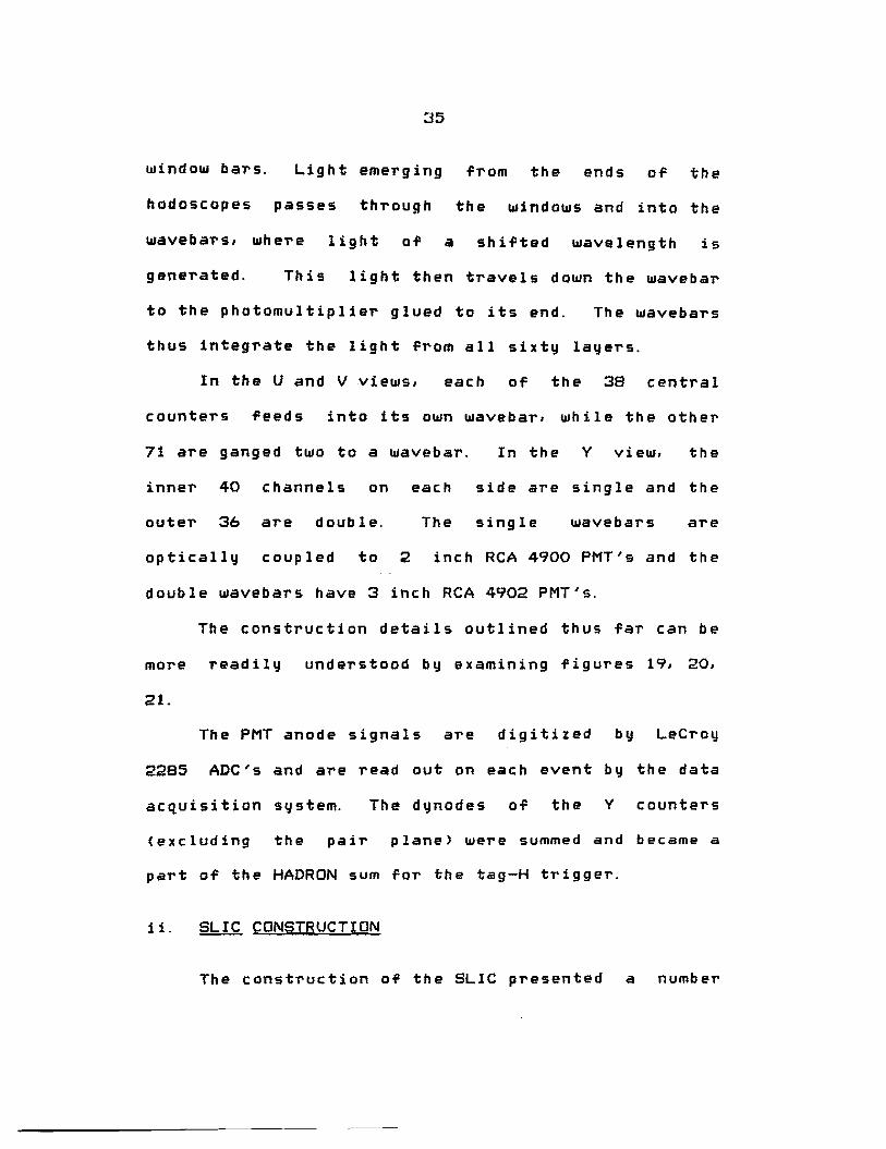
window bars. Light emerging from the ends of the

hodoscopes passes through the windows and into the

wavebars, where light of a shifted wavelength is

generated. This light then travels down the wavebar

to the photomultiplier glued to its end. The wavebars

thus integrate the light from all sixty layers.

In the U and V views, each of the 38 central

counters feeds into its own wavebar1 while the other

71 are ganged two to a wavebar. In the Y view, the

inner 40 channels on each side are single and the

outer 36 are double. The single wavebars are

optically coupled to 2 inch RCA 4900 PMT's and the

double wavebars have 3 inch RCA 4902 PMT's.

The construction details outlined thus far can be

more readily understood by examining figures 19, 20,

21.

The PMT anode signals are digitized by Lecroy

2285 ADC's and are read out on each event by the data

acquisition system. The dynodes of the Y counters

<excluding the pair plane> were summed and became a

part of the HADRON sum for the tag-H trigger.

ii. SLIC CONSTRUCTION

The construction of the SLIC presented a number

36

of challenges since a shower detector of this type had

never been built before.

Before construction, extensive testing took place

to determine what materials might degrade the

scintillator. and to ensure that a good attenuation

length could be obtained. Aluminum, stainless steel.

teflon. lucite were used exclusively in the

construction. with the exception of the a-rings, which

were of Viton.

All the corrugations started as flat aluminum

sheets, to which adhesive-backed teflon tape was

applied with a tape-laying machine. This device

removed the mylar release layer from the tape and

replaced it back on top of the teflon surface while

pressing the adhesive layer to the aluminum. The

release layer remained in place until the final

assembly and did much to preserve the delicate finish

of the teflon. After application of the teflon. the

corrugations were made on a pneumatic brake with a

specially prepared aluminum die. The corrugations for

each u, v, and Y layer were cut to size with a

high-speed table saw and set aside as a package until

needed. The U and V channels each had a mirror at the

end opposite the wavebar to increase light output.

37

These were made by means of a special punch press

which cut a flap of the corrugation material and bent

it down into the channel at a 90 degree angle to the

channel. After corrugations were cut to size, they

went to the mirror punch where this operation was

done. The Y layers are divided in half vertically by

strip mirrors, and have wavebars on both sides of the

SLIC. More details on the design and construction of

the SLIC and of a prototype can be found in references

(37. 38).

The Pb-Al laminates were made by first laying out

the bottom aluminum layer on a suction table. ·applying

a layer of adhesive, rolling out the lead layer on top

of this, followed by another adhesive layer, and

finally the top aluminum layer. The lead sheets were

cut 1" undersize so that a 1" aluminum strip could be

inserted around the edges. Epoxy was also applied

here, to ensure no delamination, and to prevent

scintillator from contacting the lead. The laminates

were then routed to exact size using an 8 by 16 foot

routing template.

Once completed. the laminates were transported to

the taping table using an array of suction cups lifted

by a fork-lift. On this table the teflon tape was

:-ta

applied using another

the back of the sheet,

tape-laying machine. To tape

the table would be tipped

vertically, then a lifting bar affixed to the top, and

the sheet picked up with a crane, flipped over, and

put down on the table again.

When the taping was complete. the laminate was

picked up by crane and carried to another tilting

table where the corrugations were attached. Pre-cut

pieces were arranged on the table, which had alignment

marks around its periphery for positioning them

properly. One by one, the corrugations were clamped

down in place by non-marring clamps. rivet holes

drilled with a high-speed aircraft drill <with a

vacuum cleaner- to suck away the chips), and the

corrugations riveted down using a standard pneumatic

rivet sq,ueezer. When all the corrugations were

riveted down, the table was again tipped vertically,

and the laminate lifted by crane and placed into the

tank.

Using shifts of 5 to 7 student workers 24 hours a

day, construction took several months.

iii. ~ CALIBRATION

For good reconstruction efficiency and mass

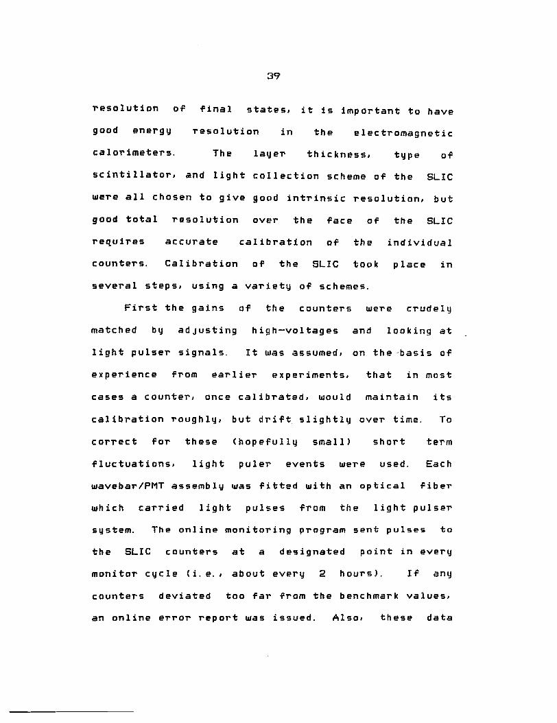
39

T'esolution of final states, it is important to have

good energy

ca 1 or imeters.

resolution in the electromagnetic

The layeT' thickness, type of

scintillator, and light collection scheme of the SLIC

were all chosen to give good intrinsic resolution, but

good total resolution over the face of the SLIC

accurate calibration of the individual requires

counters. Calibration of the SLIC took place in

several steps. using a variety of schemes.

First the gains of the counters were crudely

matched by adjusting high-voltages and looking at

light pulser signals. It was assumed, on the ·basis of

experience from earlier experiments, that in most

cases a counter, once calibrated, would maintain its

calibration roughly,

correct for these

but dri-flt slightly over time. To

(hopefully small> short term

fl uc tuat ions, light puler events were used. Each

wavebar/PMT assembly was fitted with an optical fiber

which carried light pulses from the light pulseT'

system. The online monitoring program sent pulses to

the SLIC counters at a designated point in every

monitor cycle (i.e., about every 2 hours>. If any

counters deviated too far from the benchmark values,

an online error report was issued. Also. these data

40

were written to tape, and were subsequently analyzed

by the offline monitor and written out in run-number

indexed calibration files for use by the calorimeter

reconstruction program.

The pedestals were handled in a totally analagous

way, except here, instead of a light pulse, the

monitor program simp.ly issued a false gate to the

ADC's between spills. These quantities too. were

monitored online

calibration files.

and also made into off line

The initial GeV/count calibration constants for

the SLIC were obtained in a special 5 GeV electron run

taken very early in the running period. In this

process, the electron beam was tuned to 5 GeV and a

special gymballed steering magnet was installed in

place of the target. With this magnet it was possible

to steer the 5 GeV beam over almost the entire face of

the SLIC, and thereby generate calibration data for

each counter at several positions along its length.

Because of difficulties in tuning the beam to 5 GeV,

because the SLIC PMT's and ADC's were not well

debugged before this run, and because the light pulser

system was not completely understood at the time of

the run, this data ultimately only gave a starting

41

point for the calibration. CThis data was also used

to confirm the attenuation lengths measured in the

muon calibration, discussed below. >

Most of the U and V counters were calibrated by

using tracked e+e- pairs produced by non-hadronically

interacting photons in the target. These pairs are

produced with essen~ially no P+ and are simply bent by

the magnets and lie in a horizontal plane through the

middle of the spectrometer. The corner U and V

strips, as well as all but 2 of the Y counters do not

cross

way.

higher

the pair plane and cannot be calibrated in this

Since the intensity of pairs is tremendously

near the beam axis than near the edges, it was

necessary to install a special trigger requiring at

least one electron track within 2 feet of the edge of

the SLIC. This was done by placing 2 foot paddle

counters on either side of the SLIC, in coincidence

with the normal pair trigger, which used a fan-in of

the central 3 SLIC Y counters on either side. Most or

the events coming in on this trigger actually turned

out to be 2 pairs from multiple bremsstrahlung with a

high energy pair creating the pair-plane part of the

trigger, and a lower energy track hitting the paddle

counter.

42

A unique, non-iterative method was devised for

generating the calibration constants of these U and V

counters. Suppose an electron hits the SLIC at

horizontal position x <measured in counter widths>,

and that the energy in it's shower in a small region

dx' located at x', is given by E<x'-x>dx'. Clearly,

-()()

! E(x'-x) dx' = E 00

with E the energy of the electron. The amount of

energy E1 < x > measured by SLIC counter I, centered at

x", <see figure 22a), will be given by

EI (x) f x"+.5 = A1E(x'-x) dx' x"-.5

where is the calibration constant of this

counter.to be determined. Suppose we now form the

quantity CI by integrating Er <x>IE over all possible

positions of the electron:

-oo EI (x) c1 = f 00 dx E

-co rx' •+. 5 = I dx co x"-.5

E(x'-x) dx' A1--=E--

43

1x11+.5 -oo E(x'-x) c, = dx' f 00

dx Al E x"-.5

= rx"+.5 dx A1 x"-.5

c, =

Thus, the integral we have formed is exactly the

calibration constant we want. The function Ez <x>IE

is simply obtained by calculating the average pulse

height divided by track energy for several bins in

distance from the center or the counter. The

calibration constant is then Just the integral of this

function. The shape of this function for a typical

counter is shown in figure 22b.

This method has several attractive features.

First, it is "diagonal", i.e., the calibration of one

counter does not depend on those of its neighbors.

For this reason, it is not necessary to solve for the

constants with an iterative approach. Second, it does

not depend on an explicit knowledge of shower shapes

and how they change with track angle. The integral of

such a shape is always Just equal to the energy.

44

Third. it allows all the data to be used. Tracks

which do not actually hit a particular counter can

still be used to calibrate it.

Special pair runs were taken at intervals of

about a month. Analysis of the first 7 such runs

showed that the calibration constants did not change

with time in the vast maJority of counters, within

errors of the pair calibration method (about 27.>.

This indicated that not only was the pair calibration

method working, but also that the light pulser system

was correctly tracking the gains of the phototubes,

since the pairs provided and abolute baseline-to check

against. With the light pulser corrections left off,

it was found that the calibration constants were not

very much different, indicating that the drifts were

smal 1.

The Y counters, and those U and V counters which

do not cross the pair plane, were calibrated with

background muons. These are minimum ionising and

d e p o s i t t y p i ca 11 y . 5 Ge V i n a SL IC c aunt er. Sp e c i a l

muon calibration runs were taken from time to time

throughout the run for this purpose <and also to

calibrate the hadrometer). The constants for these

counters were adJusted so that all minimum ionising

45

peaks fell at the same value. These data were also

used to find the attenuation constants of the SLIC

counters.

Further calibration was

isolated electron showers

possible

in the

using tracked

SLIC. The track

momentum calibrates the energy scale, and one further

requires that u, v, and Y views give the same energy.

Finally the mass of the pi-zero from

reconstructed can be used to set an overall energy

scale for the entire detector.

The energy and position resolutions of the SLIC

for isolated electromagnetic showers are 127./fE and 3

millimeters, respectively. For typical reconstructed

events, the energy resolution was about 157./fE.

b. OUTRIGGERS

i. COUNTERS

The outriggers, so named because two long

counters straddle the beamline, measure the positions

and energies of photons and electrons at large angles

to the beam, which are outside the vertical acceptance

of the SLIC. They can also provide an energy deposit

value for other incident particles if necessary. The

location of these counters is shown in figures 23 and

46

24.

The outriggers do not reduce the acceptance of M2

to charged

location is

spectrometer

tracks substantially.

a conse~uence of the

is divided. roughly,

Rather, their

fact that the

into a "high"

momentum part and a "low" momentum part. Low momentum

particles typicall~ emerge from the targer at larger

angles, and those with e~ ~ 40 mr will hit the

outriggers. It would have been unfeasible to make

magnet apertures and detector sizes large enough to

handle the highest and lowest momentum particles

simultaneous 1 y.

The construction of the outriggers is shown in

figure 25. They consist of two identical modules, one

above the beam and one below, each of which has 16

layers of 1/4 inch lead interleaved with 16 layers of

plastic scintillators for a total of 18 radiation

lengths. Eight of the

divided into 23 vertical

layers, called X layers are

optically isolated strips,

which feed into wavebars and PMT's Just as on the

SLIC. The 8 Y layers are comprised of 15 horizontal

1.25 inch strips. The protruding ends of the 8

scintillator strips of the successive Y layers were

formed into light guides which are coupled to PMT's.

47

All PMT's are 2 inch RCA 4900's, and had 14 mil

conetic magnetic shields. followed by iron Jackets, to

protect them from the fringe fields of M2. The anode

signals are read out with LeCroy 2280 ADC's by the

data acquisition system, and the dynode signals are

summed and added into the HADRON sum in the low level

trigger 1 og i c.

ii. OUTRIGGER CALIBRATION

Most Of the outrigger calibl'ation was done using

the background muon f 1 u x' in special muon runs. This

data was analyzed off line to establish gains and

attenuation constants for the counters. There were

also a .Pew electron runs in which the outriggers were

lowered into the electron beam of known energy. The

outriggers were also monitored online by the light

pulser system.

5. RECOIL DETECTOR

a. RECOIL SPECTROMETER

The recoil detector. a set of PWC's and

scintillator layers of cylindrical geometry

surrounding the hydrogen target. was used to determine

four-vectors of tracks emerging at large angles from

48

the hadronic vertex, as well as to provide signals to

the trigger processor for generating recoil triggers.

A particle emerging from the target will first

pass through 3 cylindrical PWC 's, each with

longitudinal anode wires for determining azimuthal

angle, and circumferential cathode wires, which

measure polar angle .. The particle then enters the

scintillators, called the A, B, c, and D layers, which

are divided into 15 compartments, called sectors, in

azimuth, each of which sub tends 22. 1 degrees. The A

and B layers are of plastic scintillator, while C and

D are actually comprised of compartments filled with

liquid scintillator. A sixteenth sector is

uninstrumented and houses support members for the

PWC's and scintillator tank, as well as PWC readout

cab 1 es. This sector introduces a dead region of 24. 5

degrees, so that the acceptance in cp is about 93/..

The lengths of the layers is about 2. 5 meters, making

the typical minimum e of recoil tracks about 25

degrees. A schematic of recoil counter construction

is shown in figure 26.

The recoil detector was designed primarily to

identify single protons from so-called diffractive

production of forward states in the -cc mass range,

i.e. about

for providing

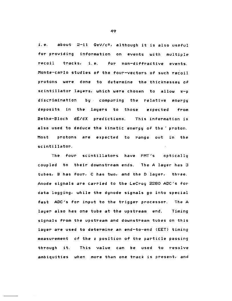
49

2-11 GeV/c2,

information

although it is also useful

on events with multiple

recoil tracks, i.e. for non-diffractive events.

Monte-carlo studies of the four-vectors of such recoil

protons were done to determine the thicknesses of

scintillator layers, which were chosen to allow w-p

discrimination by

deposits in

Bethe-Bloch

the

dE/dX

comparing the relative energy

layers to those expected from

predictions. This information is

also used to deduce the kinetic energy of the' proton.

Most protons are expected to range out in the

scintillator.

The four scintillators have PMT's optically

coupled to their downstream ends. The A layer has 3

tubes, B has four, C has two, and the D layer, three.

Anode signals are carried to the Lecroy 2280 ADC's for

data logging, while the dynode signals go into special

fast ADC's for input to the trigger processor. The A

layer also has one tube at the upstream end. Timing

signals from the upstream and downstream tubes on this

layer are used to determine an end-to-end CEET> timing

measurement of the z position of the particle passing

through it. This value can be used to resolve

ambiquities when more than one track is present, and

50

as a consistency check. The average of the time

values from the EET tubes is also used as a

time-of-flight <TOF> measurement which can help in

determining particle type for particles which stop in

the A layer.

The PWC's have a three layer construction as

shown in figures 27 and 28. The inner cathode is

aluminized mylar and is held at ground. The anode

wires on all chambers have a 4 millimeter spacing and

are stretched on a frame having two end rings with

three equally spaced support rings between them. The

inner chamber has 268 anode wires, ganged in twos, the

middle has 536, ganged in fours, and the outer has

804, gang e d i n s i x es. Thus the granularity of the

anode wires in e is the same for all three chambers.

Anode signals are processed on anode boards, sixteen

to a board. Each in-time hit wire sets a bit in a

shift register, which is read via CAMAC by the data

acquisition system. Anode wires are at nominally 2500

volts. The cathode wires are flattened copper and are

glued with 1. 5 millimeter spacing to a mylar cylinder.

Each chamber has 1312 cathode wires, which are ganged

in twos into the preamplifier-discriminators.

Typically a cluster of about 6 wire pairs will fire

51

when a track passes through the chambers. The readout

scheme calculates a centroid and width for each such

cluster and ~uickly (150 ns/cluster) sends these

values to the trigger processor for use in creating a

trigger.

The PWC's are filled with a gas mixture of 82. 5X

argon, 15X isobutan~ and 2. sr. methylal.

b. RECOIL DETECTOR CALIBRATION

The recoil detector was calibrated with single

clean recoil protons from data events. For such

events, there are no ambiguities, and the z position

measured by the cathode is used to calibrate EET. The

kinetic energy measurements are calibrated by

comparing the observed pulse heights to Bethe-Bloch

predictions for different mass and kinetic energy

hypotheses in an iterative process which ultimately

produces a set of 12 calibration constants for each of

the 15 sectors. There are three constants per layer,

which are basically an overall additive constant, an

overall multiplicative constant, and an attenuation

length. The recoil trajectory and results of energy

reconstruction are used to predict the time-of-flight

value, which is used to calibrate the measured TOF

values.

52

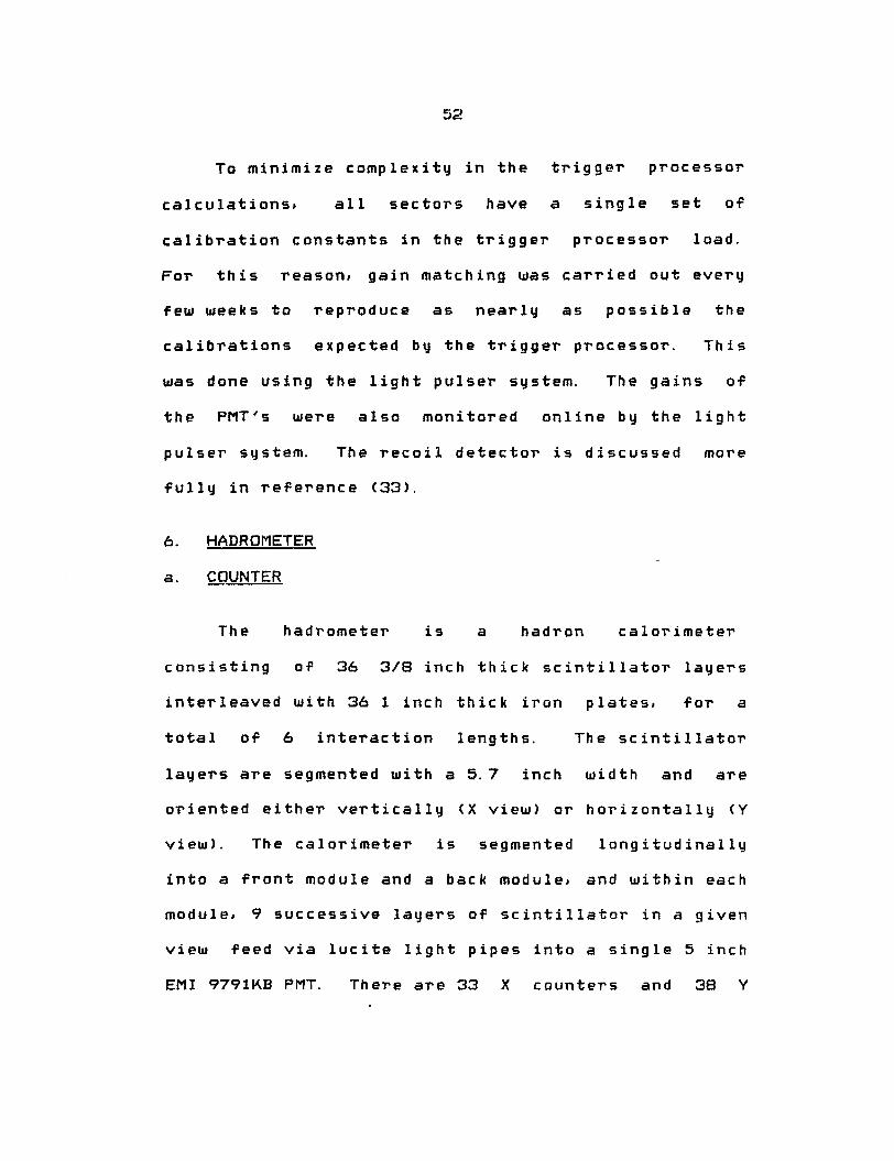
To minimize complexity in the trigger processor

calculations, all sectors have a single set of

calibration constants in the trigger processor load.

For this reason, gain matching was carried out every

few weeks to reproduce as nearly as possible the

calibrations expected by the trigger processor. This

was done using the light pulser system. The gains of

the PMT's were also monitored online by the light

pulser system. The recoil detector is discussed more

fully in reference C33>.

6. HADROMETER

a. COUNTER

The hadrometer is a hadron calorimeter

consisting of 36 3/8 inch thick scintillator layers

interleaved with 36 1 inch thick iron plates, for a

total of 6 interaction lengths. The scintillator

layers are segmented with a 5.7 inch width and are

oriented either vertically ex view> or horizontally CY

view>. The calorimeter is segmented longitudinally

into a front module and a back module, and within each

module, 9 successive layers of scintillator in a given

view feed via lucite light pipes into a single 5 inch

EMI 9791KB PMT. There are 33 X counters and 38 Y

53

counters <19 each side> in each module. The location

of the hadrometer in the spectrometer is shown in

figure 24, and its construction in figure 29.

In construction of the hadrometer, first the

steel plates were welded in place, and then the

completed 9-layer scintillators were inserted as

uni ts.

The phototube

Lecroy 2280 ADC's,

anode signals are read out by

become part

trigger.

of the

while the dynodes are summed and

HADRON fan-in for the tag-H

In the data analysis, the hadrometer provides a

measurement of the

showers. Because of

energy and position of hadronic

the intrinsically poor energy

resolution of hadron calorimeters, Cin this case,

7 5 'Y. I~ > , th e en erg y info r ma t i on i s use f u 1 on 1 y w h en a

crude number is adequate, e. g. ' for the hadronic

trigger, or to differentiate hadrons from muons, which

are minimum ionising and deposit about 2 GeV. Also,

the hadrometer positions can be matched with charged

tracks, and the hadrometer is the only source of

energy and position information for neutral hadrons.

b. HADROMETER CALIBRATION

54

The online program generated light pulser events

to monitor the PMT gains and pedestal events to

monitor pedestal shifts. These events were also

written on tape and analyzed offline to create

calibration files for use by the reconstruction

programs.

The absolute gains and attenuation functions of

the counters were established by using data from

periodic muon runs. and also a few special runs with a

tuned pion beam.

7. CERENKOV COUNTERS

a. COUNTERS

Pions. kaons, and protons identification in the

forward spectrometer is effected by two threshhold

Cerenkov counters. called Cl and C2. The location of

the counters are apparent from figure 24, while the

counters themselves are detailed in figures 30 and 31.

Information on dimensions. mirror sizes, gas mixtures.

and particle threshholds is given in tables II and

III. For momenta from 5 to 20 GeV/c, pions are

distinguishable from kaons and protons. For momenta

from 20 to 36 GeV/c, all three types of particles are

distinguishable. From 36 to 69 GeV/c, protons are

55

distinguishable from pions and kaons.

The Cerenkov counter bodies are constructed of

1/4 inch aluminum I beams. The upstream end of Cl

extends inside the field region of Ml and is made of

fiberglass to prevent damage from eddy currents. The

location of Cl necessitates a 2-bounce optics system.

The optics for Cl and C2 are illustrated in figure 32.

The upstream and downstream ends of both counters are

sealed by thin flexible windows of vinyl and aluminum

laminate. Both counters were mounted on rails to

allow positioning and removal. The Cerenkov mirrors,

which were slump-molded from acrylic sheet and

aluminized, are suspended by dacron filaments. In C2,

a 3 centimeter gap is left between the upper and lower

halves of the mirror plane to avoid collecting light

from the pair plane. The mirror segmentation and

suspension systems are shown in figure 33.

The winston cones for light collection are made

of epoxy. These are mounted on 5 inch RCA 8854 PMT's

whos anode signals are digitized by Lecroy 2249 ADC's

and subsequently logged onto tape.

signals are used in the dimuon trigger

special test triggers.

b. CERENKOV CALIBRATION

Al so,

and

the dynode

in other

56

The index of refraction of C1 was monitored using

a gas chromatograph. In C2

determined using reconstructed

determine ·the refractive index.

the pion threshhold,

tracks, was used to

Mirrors were surveyed in initially, and their

positions verified during the 5 GeV electron run.

Subsequently, the mirror positions were monitored

using reconstructed tracks. The winston cones were

aligned using light beams before the counters were

sealed up. The PMT's and ADC's were monitored online

with the light-pulser system. The pulser events were

also written on tape and used to create calibration

files for the reconstruction programs.

8. MUON WALL

a. tBlQ.M COUNTERS

Directly behind the hadrometer is a four foot

thick wall of steel which, together with the steel in

the hadrometer itself, is sufficient to range out all

but a small fraction of muons produced in hadronic

showers. Thus the only particles exiting the steel

wall are muons from the event vertex (or perhaps

background muons> above some minimum cutoff momentum

<about 5 GeV/c>. The muon wall is simply an array of

57

18 and 24 inch wide scintillator strips with lucite

light pipes and 5 inch EMI 9791KB PMT's. The layout

of the wall is shown in figure 34, and is discussed

again in the section on the dimuon trigger.

The signals from each PMT feed into

discriminators, the outputs of which are used to set a

latch bit, to start a TDC, and as an input to the

dimuon trigger. The TDC value is used offline to

measure the Y position of the muon hit in the counter.

b. MUON WALL CALIBRATION

The counter efficiencies were measured· with a

paddle counter telescope <triggered by background

muons> at the near end and far end of each counter.

All counters were essentially 100i. efficient near the

PMT. and typically about 987. efficient 7 feet from the

PMT. The TDC T0 's and gains were measured offline

with reconstructed tracks.

C. TRIGGERS

1. TAG-H

This trigger is the core of all the experimental

triggers. with the notable exception of the dimuon

trigger discussed below. It is a coincidence between

58

tag, which is supplied by the tagging system and

simply indicates the presence of a tagged photon. and

H, which indicates the presence of energy in the

calorimeters that is consistent with a hadronic

interaction. To form H, the dynode signals from the

hadrometer and SLIC CY view only, excluding pair

plane> are summed, in the linear combination EH=

ESLIC + 1. 25 * EHAo· The tag-H trigger required that

This is equivalent to requiring that

EH > .3*<Ee -ETOT>, where ETOT is the total energy in

the tagging system, which is in turn equivalent to

EH +.3*ETOT > .3*Ee, where .3*Ee will simpl~ become

the equivalent discriminator setting for tag-H. The

outrigger dynode sum was discriminated and or-ed in

with HADRON. The logic diagram of tag-H is shown in

figure 35. The electromagnetic backgT'ound, which is

200 times larger than the hadronic interaction rate,

was reduced to a level about equal to the hadronic

rate by use of the tag-H trigger. The efficiency of

the tag-H trigger was measured to be 97 ± 2 percent.

2. RECOIL TRIGGERS

Recoil triggers are generated by the trigger

pT'ocessor. This is a unique trigger processing system

59

which uses high-speed ECL circuitry and memory-look-up

<MLU> units to make complicated triggering decisions,

involving track finding and particle identification,

in a few microseconds. This system is discussed in

detail in references (26, 27, 28>. Basically, the

trigger processor uses information supplied to it by

the recoil spectrometer to decide if a hadronic event

Ctag-H is a prerequisite to recoil triggers> possesses

a single well identified recoil proton emerging from

the must upstream hadronic vertex. To make this

decsion, the processor actually reconstructs tracks in

the recoil PWC's, matches these with EET information

in the recoil calorimeter, and attempts to identify

the recoil particle as a pion or proton from its

energy d ep os its. When a clean proton is identified, a

missing forward mass is calculated from the

four-vectors of the incident photon and the recoil

proton. The recoil triggers are defined by:

1. Recoil 1: 0.0 < Mx < 2.0 GeV/c2

2. Recoil 2: 2.0 < Mx < 5. 5 GeV/c2

3. Recoil 3: 5. 5 < Mx < 11. GeV/c2

60

The recoil 1 trigger was heavily prescaled to allow

only small number of low mass events to be recorded

for calibration purposes. The p events, for instance,

were useful as a check of the track reconstruction

program.

The process ~~e~e- is expected to come in under

the recoil 2 trig~er since the ~ has a mass of 3. 1

GeV/cZ. The tag-H is provided by the high energy

electrons hitting the SLIC. Since this trigger is

biased heavily toward elastic production, the

dielectron mode will be used only as a crude check of

the elastic cross section. We shall return -to this

point later.

3. DIMUON TRIGGER

The efficiency of the recoil trigger for ~ is

rather low. due in large part to fact that many of the

protons have low -t and do not escape the target.

Also, the recoil trigger is biased toward elastic

production. The dimuon trigger was implemented to

allow detection of ~ at a higher rate and to provide

an unbiased ~ sample.

This trigger utilized dynode signals from the

muon wall counters to identify candidate dimuon

61

events. It consists of two parts, here called MEW <Mu

East-West> and MUTS CMUon TeleScope). MEW is designed

to pick up the more symmetric decays in which one

expects (for the elastic case> to find the muons in an

East-West or Up-Down configuration. MUTS is designed

to pick up many of the asymmetric decays where one

muon is very fast and travels down the center of the

spectrometer into MU16, and the other is slower and

hits some other muon counter. Thus, MEW is a

coincidence between the East and West sides of the

muon wall <or between MU14 and MU18,

and above the central counter),

directly below

and MUTS is a

coincidence between the central MU16 counter and the

outer muon counters. To reduce the number of

accidental triggers, a coincidence with C2 was

required for MEW, while the Pre-C and Caboose counters

served the same purpse for MUTS. The Pre-C and

Caboose counters are simply scintillator paddle

counters; their locations are shown in figure 36. The

dimuon trigger logic is:

DIMUON = MEW + MUTS

62

MEW= [(µ6+µa+µ10+µ12)·CE]·[(µ20+µ22+µ24+µ26)·Cwl

+ (µ14. CON) • (µ18 •CUP)

CE , Cw , Cup , and CON are fan-ins of the east, west.

top. and bottom counters of C2. The logic diagram for

the dimuon trigger is shown in figure 37.

D. DATA ACGUISITION SYSTEM

The data acquisition system is -outlined

schematically in figure 38. The Fermilab standard

RSX-MULTI online system provided a user-oriented

environment on the PDP11/55 in which data taking runs

could be initiated and ended, and through which a

variety of user-defined quantities could be monitored,

with graphics displays and MULTI commands.

MULTI also interacted with a stand-alone data

acquisition system which when prompted by an event

interrupt from a high-level trigger, read the data

from the detectors out of all the CAMAC modules via 3

Jorway model 411 CAMAC branch drivers. The data was

initially stor~d in a fast bank-switchable bulk memory

63

system; during the interspill period the data was

transferred to one of Tagged Photon Lab's two 6250 BPI

magnetic drives. Typically, about 50 events of all

types were recorded per beam spill.

MULTI also controlled the data monitoring

program.

1.

This program had the following functions:

calibration events Generate

pedestals, light pulser events,

chamber pulser events.

such as

and drift

2. Compare data from these events with benchmark

values stored on disk.

3. Monitor high-voltages, low-voltages, magnet

currents, mean chamber multiplicities, data

integrity for the recoil system.

system calibration, scalers, etc.

tagging

4. Generate warning messages when any quantity

was outside of acceptable limits.

64

IV. DATA ANALYSIS

A. PRODUCING THE ~ SIGNAL

During a 3 month data taking run in Spring of

19811 at an electron beam energy of 170 GeV, 7592374

triggers of all types were written onto 255 6250 BPI

tapes. This data set represents . 994E11

live-time-corrected tagged photons on target. All

tapes were run through two sequential analysis passes

on the Fermilab CYBER 175's. In Pass-1, the dT'ift

chamber charged

analysis, part of

track reconstruction, recoil counter

the Cerenkov reconstruction, and

part of the tagging analysis were carried out. Each

raw data tape created three partially full Pass-1

output tapes to allow room for additional Pass-2

information. In the second pass, the electromagnetic

and hadronic calorimetry analysis were carried out, as

well as the remainder of the Cerenkov and tagging

analysis. Particle identification, using the Cerenkov

for w/K/p, and the calorimeters and muon wall for µ

and was also done. The electron and muon

identification programs are discussed more fully

later. Each Pass-1 segment (1/3 of a raw tape) was

used to create one Pass-2 output segment <which still

65

retained the raw data>. At this stage the main-line

data reduction was complete and the tapes could be

stripped to look for specific physics signals.

A stripping program was written to select both

dimuon and dielectron candidates from the Pass-2

ouptut tapes and write

files. The stripping

them onto special

selected roughly

candidates and 150 dielectron candidates,

condensed

120 dimuon

out of a

total of some 30000 beam events, from each complete

three-segment Pass-2 output tape. Cuts were left

rather loose on this initial stripping pass.

outlined below.

They are

For dimuon candidates. at least one pair of

tracks had to exist which satisfied the following

cuts:

1. Opposite charge

2. Distance of closest approach of the two

tracks less than 2 inches.

3. Position of closest approach within beam

spot.

66

4. Invariant mass greater than . 5 GeV/c2 <to

reduce the number of low mass background

events written out>

5. Total momentum of two tracks at least 30/. of

tagged photon energy.

6. At least one of the tracks flagged as a muon

in Pass-2.

7. The other track, if not so flagged, must have

an energy deposit in the hadron calorimeter

which is consistent with minimum ionising.

Cut 5 could introduce a bias in the z distribution,

but, as we shall see, the efficiency for z < . 4 is ,.,,

essentially zero anyway.

A track was identified as a muon in Pass-2 if

1. A muon counter gives x Cflrom counter

position> and y <from TDC> consistent with

track position at muon wall.

2. Hadrometer energy deposit is consistent with

67

minimum ionising in magnitude.

front-to-back ratio.

width, and

In the final analysis, only 4Y. of dimuon tracks had

not been flagged as muons in Pass-2, indicating that

inefficiencies in the muon identification technique

were small.

For dielectron events, the cuts used were:

1. At least two tracks are consistent with being

electrons based on the ratio of SLIC energy

to drift chamber momentum, and, for tracks

below 20 GeV, based also upon shower width in

the SLIC. Four-vectors of photons consistent

with being bremsstrahlung photons radiated by

the electrons are added in to the

four-vectors of the corresponding electrons.

2. Neither electron consistent with being from a

beam pair Ci. e. ' Bethe-Heitler

electron-positron pairs from photons that did

not interact hadronically in the target>.

3. Each track has~ 6.0 GeV/c momentum.

68

4. Total momentum of the two electrons is at

least 304 of the tagged photon energy.

5. Invariant mass of electron pair is at least

. 5 GeV/c2.

A clear signal was seen in both dimuon and

dielectron channels after the initial stripping pass,

but backgrounds were still rather large. When the

stripping pass was complete, the stripped events were

copied onto summary tapes. Then a ~ analysis program

was run on these tapes, which attempted to reduce the

background by more cleanly identifying muons and

e 1 ec trans.

The additional new cuts for the dimuons were:

1. Total momentum of two muons less than 220

GeV/c <to get rid of tracks with mis-measured

momenta>.

2. Distance of closest approach less than .4

inches.

3. Tighter cut on veT•tex position.

69

4. SLIC energy less than 2. 2 Gev for each track

(i.e., consistent with minimum ionising; the

minimum ionising peak is at about . 5 GeV,

with a Landau tail that is significantly

populated out to 2 GeV or so. >

5. Each muon has momentum greater than 9 GeV/c.

6. <Calorimeter energy>l(Drift Chamber momentum>

is less than .3 for each track <to cut out

low energy pions that might be identified as

muons>

7. Less than 9 good tracks besides the 2 muons.

8. If more than one pair of tracks pass all

cuts, take the highest energy pair.

The final vertex distributions are shown in figure 39.

These distributions are quite clean: the widths of the

x and y distributions are comparable to the beam size,

and the z distribution cuts off fairly cleanly at the

front and back ends of the target. The sum of al 1

cuts had an estimated efficiency of . 93 ± . 05,

70

determined by estimating the number of ~'s above

background before and after making the cuts. This is

discussed again in the section on efficiencies. The

final dimuon mass spectrum is shown in figure 40.

There are 147 events in the range 2.8 ~ M<µ+µ-> < 3.4

GeV/c2.

For die 1 ec tron.s, in the background reduction

program, more stringent cuts were made on the ratio of

SLIC energy to drift chamber momentum, and the shower

widths of all candidates were required to be

consistent with being electromagnetic. The overall

efficiency of all cuts was estimated to be .92 ± .05.

The final dielectron spectrum is shown in figure 41.

For the d imuons, it was found that requiring a 11

events ta have the dimuon trigger bit an did not

affect any events with dimuon masses above 2.4 GeV/c2.

This cut was then made permanent.

After the background reduction pass, events were

written onto small disk files for further analysis.

B. DEFINITION OF ELASTIC AND INELASTIC

After the ~ signal was isolated, programs were

run wh i ch classified each event as elastic or

inelastic. Since the dielectrons must came in on a

71

recoil trigger, this sample is biased strongly toward

diffractive production, and therefore, in the absence

of a detailed monte-carlo study of recoil trigger

acceptance for non-diffractive events, it is not

useful for a comparison of the relative magnitudes of

elastic and inelastic cross sections. Rather, the

totally elastic dielectron events are used as a crude

check of the dimuon cross sections, as will be

discussed along with the final results. In what

follows. then, we refer only to the dimuon case in

discussion of elasticity assignment. <In fact. a

totally analogous procedure was followed ·for the

electrons in defining their totally elastic sample.>

For our purposes, only the exclusive process

lP~~p is considered to be totally elastic production.

Inelastic production, from a physics standpoint

encompasses three classes of processes. namely,

1. lP~~N*• the so-called quasi-elastic process.

2. lP~~*P, with ~*7~X, where charmonia are

produced elastically and subsequently decay

to ~' and

72

3. 1p.+q1X, the truly inelastic,

process.

hard scattering

From a theoretical standpoint, though, it is

desireable to focus on the third process, i.e., truly

inelastic production. As we shall see. the first

process can be excluded by means of a cut in z = E~ /Ey , and the second process can be "subtracted

out", roughly, in a statistical way, even if it is not

possible to completely reconstruct the events in all

cases.

Operationally,

inelastic if

an event is classified as

1. Real forward tracks, photons, or hadronic

neutrals are detected accompanying the ~

(forward inelastic),

2. The recoil system data is inconsistent with

the single recoil proton calculated from the

incident photon and ~ assuming elastic

production <recoil inelastic>.

The remaining events are called elastic.

73

C. CLASSIFICATION OF EVENTS

1. FORWARD CLASSIFICATION

The forward inelastic classification

accomplished in a subroutine called CHOOSE.

was

It was

necessary to apply cuts to the additional particles

detected in order to exclude backgrounds and spurious

tracks, which could have forced truly elastic events

to be labelled inelastic. The cuts in CHOOSE were:

l. For tracks:

1. Must be seen in a calorimeter.

2. Not consistent with being a beam pair.

3. Must come from near the 41 vertex.

4. Must be seen in at least Dl and 02.

2. For photons:

74

1. Energy of at least 3 GeV (to exclude

untracked muons>.

2. Not in pair plane.

3. Pi-zeroes must have a high probability of

being real based on the two-photon mass and

the possible presence of other combinations.

4. Hadronic neutrals must have energy above 9

GeV <to exclude untracked muons>.

The motivation for these cuts, and their effect on the

data are discussed in the section on uncertainties in

assignment of events.

In figures 42 and 43 we present separate mass

plots for forward elastic and forward inelastic

events. The elastic and inelastic plots have 110 and

37 events, respectively, in the mass range 2. 8 s;_

M <µ+ µ- > < 3. 4 GeV/c2. The cl ear peak in the forward

inelastic plot is conclusive evidence of inelastic ~

photoproduction.

2. RECOIL CLASSIFICATION

75

All forward elastic and inelastic events were

also assigned as recoil elastic or inelastic by

examining the data from the recoil spectrometer. We

make the ansatz that the detected 41 was produced

elastically. Using the measured four-vector of the 41,

constrained such that E2 = p2 + M2, and the 141 \jJ \jJ

approximation E-y = E141 which is more accurate than

the tagging energ1:4 for elastic production, we

calculate, b1:4 imposing momentum and energ1:4

conservation, the polar angle, e, azimuthal angle qi,

and kinetic energ1:4 T of the recoiling proton. The

errors in track momenta and slopes are also used to

compute the errors predicted in e, ~· and T.

It should be stressed that in the recoil

classification, the four-vector of the recoil proton

is calculated using only the 41i no other forward

particles <if present> are included. This method has

the advantage that if forward tracks are missed, the

event will still be classified as inelastic since the

recoil proton will not match up. The disadvantage is

that elastic charmonimum production will also be

called inelastic since we do not include the extra

tracks along with the ~ from the charmonium decay.

There is really nothing that can be done about this

76

situation since it was not possible to totally

reconstruct all the events. Thus there is an unknown

amount of elastic charmonium production in our

inelastic sample. There are, however, two points that

mollify this problem: 1> Most of the inelastic forward

events can be clearly identified as inelastic in the

recoil system <and therefore not from charmonium

production> because of the presence of extra tracks in

the recoil system. 2> The ~, cross section is known.

~, production can be "subtracted out" approximately in

a statistical way, as we shall see.

During the data processing, a standard recoil

reconstruction package had been run on every event.

This provided e, $1 and momentum values, as well as

particle identification information

tracks in

.Por all .Pully

reconstructed

spectrometer.

neutrals was

cathode <e>

charged the recoil

Information on unmatched tracks and

also provided. This program matched

tracks to anode <$> tracks by attempting

to find an end-to-end-timing CEET> value in some

sector which agreed with that predicted form the

cathode track. The particle's type and momentum were

determined from its energy deposit in the scintillator

layers. The errors on measured quantities were also

77

provided. In a large fraction of the events, these e,

~· and T values could be directly compared to those

predicted from the ~· Because of PWC inefficiency and

noise, fau 1 ty data read out, interactions in the

scintillator.· confusion from background tracks or real

extra tracks, and because the recoil program did not

know the IP vertex position a priori. the information

from the recoil reconstruction program was not useful

in some cases. For this reason an event display

showing raw PWC hits, scintillator

EET values. forward vertex position,

quantities was made for each event,

energy deposits.

and the predicted

and these were

hand-scanned. The kinetic energy reconstruction was

run again on each event using the predicted sector of

the proton, and this information was also printed out

on the event display. Knowledge of the vertex and

predicted e and ~ allowed 2-hit tracks. which the

reconstruction program did not always find,

picked up.

to be

In comparing the predicted with measured

quantities an overall error was calculated as the sum

in quadrature of errors

quantities. The size

on

of

predicted and

the errors on

quantities depends on the measurement errors

measured

predicted

of the

78

forward tracks, however typical values are

1. <1 e (pre d ) ... 30 mr.

2. <r0

<meas> "' 20 mr.

3. <r~<pred> - 100-200 mT'. Csector=380 mr. >

4. <r~Cmeas> "'40 mr.

5. <rTCpred> "'257. CT~ 40 MeV; worse below>

6.

In cases where the standard reconstruction package

failed, the error in the measured recoil ~uantities

was assumed to be the average error. Recoil tracks

clearly emanating from the forward vertex were

compared to the predictions.

inelastic if:

Events were labelled

1. At least 2 of e, q,, T were off by 2cr or more.

or

79

2. At least one of o, cp, T were off by 3<r or

more.

3.

ID:

No recoil proton is

should not have ranged

This is rare.

seen even though it

out in the target.

4. A matching track is seen but there is clear

evidence of an additional track<s>.

al so rare.

This is

The remaining events are called recoil elastic, and

consist of two types:

1. A matching recoil track is found.

2. The recoil proton is predicted to range out

in the target and none is seen. A kinetic

energy of roughly 30 MeV or more is necessary

for a proton to Just reach the A scintillator

layer. For about 36/. of the totally elastic

events, (elastic in recoil and forward

80

systems), the recoil proton ranges out before

reaching the A layer.

D. DETERMINATION OF i..

After an event was labelled inelastic by CHOOSE,

a modified version of CHOOSE. called OMNES, was used

to calculate the four-vector of all forward particles

excluding the ip. The energy component of this

four-vector can now be used to compute z through

where Ex<1> is the energy component of the

four-vector. The cuts used in OMNES were identical to

those in CHOOSE with two exceptions:

1. Tracks are no longer required to be seen in a

calorimeter.

2. The photon energy cut was lowered to 2.2 GeV

from 3. 0 GeV.

It was assumed that. for truly inelastic events.

81

errors introduced by possibly spurious particles, due

to the looser cuts, would be small in most cases in

comparison to the total inelastic energy. A photon

energy cut of 2.2 GeV will exclude all but a few

percent of background muons while now allowing real

photons in the range 2.2 to 3.0 GeV to be included in

the total inelastic energy. OMNES thus allows the

best possible estimate of the detectable forward

energy. The "raw" z distribution from OMNES was

plotted l> with cuts as described above, and 2) with

cuts identical to those in CHOOSE. The change in the

z distribution was actually rather slight. The

distribution for 1> is shown in figure 44a.

In principle the tagged photon energy can be used

to calculate z by the formula

z Eiµ

= ETAG

The resolution of ETAG is, however, about 6.87.,

would give a sigma of 6.8 GeV for a 100 GeV ~·

which

For a

z of .9 at 100 GeV, the total inelastic energy is only

10 GeV. Thus, the use of the tagging energy is

undesireable at high z since 1) the fractional error

82

in <1-z> is large and 2> the calculated z may be

larger than one, creating an ambiguity with elastic

events.

There are also problems with using Ex Cl> from

OMNES to calculate z. Although the tagging energy is

too inaccurate for calculating z at high z, it was

possible, by averaging over a number of events, to use

it to determine that on average, only about 54/. or the

total inelastic energy was being detected. This can

be seen by comparing figures 45a, 45b, and 45c. In

figure 45a, the ratio A = E~ /ETAG is histogrammed for

elastic forward events. The mean is 1. 052 :I: .-010, in

good agreement UJi th the known systematic 5/.

underestimate of the electron beam energy. In figure

45b, we plot B = E iJ; /ETAG for those inelastic forward

events that satisfy Ex<l> < 2 * .068 * ETAG, i.e., we

exclude the events with the largest values of Ex<l>.

This was done to prevent the introduction of

uncertainties due to possibly large fluctuations in

the detected energy Ex<l>. The mean of this plot is

. 905 ± . 022. The inclusion of all inelastic forward

events does not significantly change the mean. In

figure 45c, C = CE~ + Ex<l>>IETAG is plotted for the

same class of events as in figure 45b. The mean is

83

. 985 ± . 019. Again, the mean does not change

appreciably if all events are included. The ctuantitiy

C-B Qabc = A-B

is a measure of the mean fraction of the total

inelastic energy that is detected. The result is Gabe

= . 544 ± . 1 51. Taking the inverse of Gabe we see that

to calculate z using Ex<l> we should scale it up by a

factor F = 1.84 ±. 51. The error here is JUst the

error on the mean factor. We expect a considerable

spread in this factor on an event by event basis. If

we assume that the mean of this spread is about half

the correction, we obtain F = 1.84 ± 1.05. Thus we

can calculate z by

This method will work best when Ex<l> is small

compared to the error in the tagging energy.

In practice, z was calculated using whichever of

the two methods had the smaller predicted error. The

condition z ~ 1 never occurred. The ETAG method was

84

employed for smaller z values, and the Ex<l> method

near z = 1. The resulting "corrected" z distribution

is shown in figure 44b.

Information on the energies of recoil particles

is not reliably known. We can, however, estimate the

effect of these on the z value. <This is necessary

only for forward elastic events since the energy

missed in the recoil was included in the correction to

Ex C 1 > >. The mean e of recoil tracks is something like

40 degrees. W i th t y p i ca 1 p + v a 1 u es of 3 50 Me VI c, th i s

indicates 540 MeV/c for recoil tracks. For

two or three such particles, we thus expect 1-2 GeV in

the recoil system. Thus, for the tf.1 energies in this

experiment, events which are inelastic in the recoil

system only can safely be assigned to the highest z

b i TI 1 • 95 < Z < 1. 0.

Since only about 547. of the inelastic energy is

detected, it is important to check that inelastic

events are not being called elastic in some instances.

The CHOOSE program tabulates the number of tracks,

photons, pi-zeroes. and hadronic neutrals which pass

the cuts for each event. These quantities are

histogrammed in figures 46a, 46b, 46c, and 46d. The

total number of extra particles Cwhere pi-zeroes count

85

as two> is shown in figure 46e. About 707. of the

events have 2 or more inelastic components. Of those

with onlc,i 1, many also had an additional track that

did not hit a calorimeter or a photonCs> below 3 GeV.

<The elastic events, though, usuallc,i showed little

evidence for additional energy which failed the CHOOSE

cuts.> It is thus unlikely that many inelastic events

are classified as elastic. Two events were somewhat

marginal, involving only a track of less than 1 GeV or

a photon near the the pair plane. This type of event

is treated in the following section on uncertainties

in classification.

E. UNCERTAINTIES IN CLASSIFICATION

1. UNCERTAINTIES IN FORWARD CLASSIFICATION

The cuts in the CHOOSE subroutine were designed

to prevent truly elastic events from being labelled

inelastic due to the presence of uncorrelated or

spurious tracks or photons. Four techniques were used

to check the effect of these cuts on the

classification of events.

First, the subroutine was run on elastic

monte-carlo data which included background e+e- pairs

86

and background muons. The number of events which were

classified as inelastic was negligeably small. Second

the photon energy cut was examined. The SLIC cut of 3

GeV and hadrometer cut of 9 GeV ensure that less than

lX of untracked muons will be identified as photons.

based on the measured spectra of minimum ionising

particles in the SLIC and hadrometer. A plot of

photon Y position at the SLIC, outside the pair plane,

indicated no contribution from leakage of untracked

pairs outside of the pair plane. Thus. the

contribution to the inelastic events due to muon and

pair background is negligeable.

Third, a z value was calculated, using OMNES, for

events which had been labelled elastic by CHOOSE. Of

the 110 elastic forward events, 4 had z :F 1.0. with

the mean z of these 4 being .98. Thus, z "' . 98 can be

thought of as the "inelastic threshhold" for this

experiment, above which elastic and inelastic cannot

be reliably distinguished. In the forward inelastic

sample, 2 events had z > - . 98, fl or a total of 6

"marginal" events. The recoil system. however,

resolved the ambiguity in 4 of these cases, labelling

these events as inelastic, and thus leaving 2 events

with potentially incorrect classification. Clearly.

87

for z ~ . 98, in those cases where the deviation from

elastic in the recoil system is less than our

resolution, we can make no statement about incorrect

classification: these events must simply be called

elastic. However, we may estimate that for events not

too far from inelastic threshhold, the probability of

misidentification is about 50%. Thus we might expect

that rather

mi sid enti f i ed.

than 2,

To

perhaps 4 are potentially

reflect this additional

uncertainty, the errors on numbers of elastic and

inelastic forward events are increased by half this

amount, or 2 events. This contribution ·is much

smaller than that of the statistical errors. The

numbers of events and their errors are discussed more

fully in the final results section.

Finally, the 5 events which were found to be

inelastic forward but elastic in the recoil were

examined more closely to see if they might possibly be

truly elastic. The largest z value of these was . 86,

indicating that they were truly inelastic

The case of ~ plus neutrals is a difficult one.

Because it was necessary to put the photon energy cut

at 3.0 GeV, events with mul~iple soft photons would be

classified as elastic. Copious production of such

88

states, then. would introduce a systematic error in

our inelastic and elastic fractions. A known source

of such events is the process ~p~~,p~~nonop. Using

the ratio u<~>/uC~'> = .20 % .05 C15> and the

branching fraction for ~,~~nowo of 17/. we predict

about 3 events. A monte-carlo calculation gives a

mean z of . 84 for th.ese events. At a photon energy of

100 GeV. this gives 16 GeV to be shared among 4

photons. Thus it is unlikely that even these events

would be classified elastic.

As a rough check of the inelastic reconstruction

efficiency, a search for ~, production ~as made.

Using the previously quoted cross section we predict 7

events in our inelastic sample into ~n+n-, where we

have included the reconstruction efficiency for the ~

but not the additional pions. In figure 47 we

present the forward mass spectrum for events with four

tracks, total charge ze.ro, and no extra photons or

hadronic neutrals, where the muons are required to

form a ~· A peak of 4 events appears at the ~, mass

(3. 685 GeV/c2 >.

2. UNCERTAINTIES !.M RECOIL CLASSIFICATION

In about 15/. of the events, it was not possible

89

to make a clearcut decision on elastic or inelastic in

the recoil system. The reasons for this were:

1. Confusion in PWC's due to delta rays or

missing or spurious hits.

2. Protons interacting in the scintillator.

3. Errors on predicted quantities too large.

4. Recoil acceptance losses <tracks go into

missing sector or out end of counter>

5. Recoil data not present or incorrect.

6. Recoil data self inconsistent.

However. in about 2/3 of these cases. it was possible

to pick elastic or inelastic with high probability.

In the remaining cases a guess was made based on all

information available. An additional systematic error

of . 5 event was assumed for any event that could not

be assigned with certainty to either the elastic or

inelastic category.

90

V. EFFICIENCY CALCULATIONS

A. TRACK RECONSTRUCTION EFFICIENCY

A tracking monte-carlo, which attempted to mimic

the true operating environment of the track

reconstruction program by including noise hi ts,

cross-talk, and inefficiency, was used to estimate the

track reconstruction efficiency. The noise, cross

talk, and inefficiency information was obtained from a

detailed study of a small number of runs. and may only

be valid for runs in that region of the data. The

efficiency obtained was .80 % .02 (statistical> for

1p7µ.+µ.-, (i.e., about . 90 per track>. with an estimated

systematic uncertainty of about 16 percent.

To account for possible time dependence of the

track reconstruction efficiency, a study was made of p

photoproduction for the same 170 GeV data sample. A

plot was made of the number of events of the form

versus the total lP"*PP• p-+tr+n-, per flux bin

accumulated flux. This plot, in an ideal experiment,

would be flat, indicating a constant reconstruction

efficiency

central dip.

over time. Instead,

The 41 was assumed to

the plot showed a

exhibit the same

behavior, since it, too, is a two prong topolo;iy. The

91

statistics on the ~ sample are low, but there was

evidence of a central dip for the ~ too. This dip was

also seen in the same location in a plot of number of

KO per run. On the other hand, the number of no per

event, which does not directly involve the track

reconstruction, showed no dip. A correction factor

equal to the average number of p per bin divided by

the average of the largest 4 contiguous bins in the

vicinity of the Monte-Carlo model run <where the

reconstruction efficiency was presumably best> was

applied to the track reconstruction efficiency. These

factors were. 74 ± .07 for MUTS and .60 ±. 05·for MEW.

These also include the fact that the MEW trigger was

not functional for part of the run.

The p study was also used to map out the spatial

dependence of the track reconstruction efficiency. A

central inefficient region, or "hole" caused by the

high flux of beam pairs was discovered, and its extent

was mapped out by the positions of pion tracks from

the p. This hole, which was then included in the

elastic and inelastic monte-carlo's (discussed below),

reduces the ~ signal by about 10Y., after other factors

are included. The . 80 efficiency quoted above does

not include the effect of this hole.

To estimate the effect of extra tracks on

inefficiency for inelastic events, the tracking

monte-carlo was run with a ~,~~n+n- generator. This

should be adequate since, as we saw. very few of the

inelastic events have more than two additional tracks.

The presence of the extra piqns reduced the event

reconstruction efficiency by only about 3X. This

effect was then included in the inelastic efficiency.

B. ELASTIC MONTE CARLO

A monte-carlo was written with the following

attributes:

1. Bt • h 4 d <TI d t '\le w I t B= • Changing B from 2 to 20

did not measurably affect the results.

2. Vertex generated uniform in z within target.

3. ~ decays to 2 muons distributed as 1+cos20,

where 9 is measured with respect to the lab

direction of the ~ as seen in the ~ rest

frame. The data is consistent with this. the

standard SCHC prescription, but statistics

are too low to rule out other distributions.

The results have only about a 57. dependence

upon the anglular distribution used.

4. Muons are proJected through the spectrometer.

5.

All known acceptance losses and analysis cuts

are taken into account. If two muons hit

muon counters which would cause a dimuon

trigger, the event is kept.

This monte-carlo did not do tracking. The

track reconstruction efficiency was done

separately.

section.

as discussed in the previous

The MEW part of the dimuon trigger contains a

Cerenkov coincidence. This appeared to introduce an

additional inefficiency in the trigger, as the ratio

of MEW to MUTS in the data did not initially match the

monte-car 1 o. By histogramming Cerenkov light for

tracks from MEW events and those from MUTS events it

was possible to measure this inefficiency, which was

included in the monte-carlo. The final elastic

reconstruction efficiency as a function of photon

94.

energy is shown in figure 48.

C. INELASTIC MONTE CARLO

The philosophy in the inelastic monte-carlo was

not to generate events explicitly according to a

particular model, but to generate data-like events in

a simple way, determine the efficiency as a function

of k = Ey and z, and then demonstrate that the

results are insensitive to the method used.

The inelastic monte-carlo diffractively generated

forward masses from XMIN = M ljJ + 2M11' to XMAX, with a

t slope B of 4. Changing B from 2 to 20 did not

measurably affect the results. The forward masses

were generated from a distribution that fell linearly

from XMIN to XMAX. The forward mass then decays to

~n+n- where the pions decay via two body phase space.

Events generated in this way produce ~ with some P+

and z distributions. By varying XMAX, it is possible

to vary the P+ and z dependence. XMAX was chosen to

have the value 0.65X0 where X0 is the maximum

kinematically allowed forward mass that can be

produced in the reaction lP~M<X0 >p. Choosing this

value yielded a P+ vs. z distribution which agreed

95

well with that predicted by Berger and Jones (5) over

the range of z values accessible to this experiment,

as shown in figure 49. Also, the resulting P+

distribution had a mean value of . 75, which is roughly

comparable to the value .96 found for the inelastic

data <we shall return to the inelastic P+ distribution

later>. In fact the efficiency does not depend

strongly on the value of XMAX used. In changing XMAX

from 0. 5X0 to 1.0X0 , efficiency numbers changed about

20Y. near z = . 4, and very little near z = 1., in spite

of the fact that the P+ distribution extended to

unphysically large values for the case of XMAX =

1.0X0 . Using the cross section predicted by Berger

and Jones, which falls rapidly at low z, the total

predicted number of inelastic events changed only

about 107. when XMAX was changed from 0. 5X 0 to 1.0X0 .

In any case, the efficiency is not strongly dependent

upon P+• as seen in figure 50 where we present the

inelastic efficiency for two bins in P+·

The ~ was assumed to decay isotropically in its

center of mass. Berger and Jones predict a nearly

uniform distribution for high z and reasonable P+

values, where most of the data lie. Using l+cos2e or

sinze changes the results by only about 5/..

96

The dimuon trigger and reconstruction "hole" were

put in Just as for the elastic monte-carlo. The

overall inelastic efficiency is illustrated in figure

51 for several values of k. This efficiency, taken as

a function of k*z = E \jJ is almost identical to the

elastic efficiency. It differs only slightly due to

the different angular distribution used, P+ effects,

and the reduced track reconstruction efficiency for

multiple tracks. In correcting inelastic events for

efficiency, the efficiency was treated as a function

of k*z and k, since E\jJ is known more accurately than

either k or z, and since, once the Ew dependence is

factored out, the efficiency now depends only weakly

on k.

97

VI. RESULTS

Each dimuon event has now been categorized as

elastic or inelastic in both forward and recoil

spectrometers. The events are now broken down into

seven categories based upon these classifications:

1. All events.

2. Forward elastic. Any recoil configuration.

3. Forward inelastic. Any recoil configuration.

4. Forward elastic, but recoil inelastic.

5. Forward elastic and recoil elastic,

totally elastic.

i. e. ,

6. Any inelastic, i. e. , forward inelastic and/or

recoil inelastic.

7. Inelastic with z ~ .9. This by definition

excludes recoil inelastic.

?8

In each category, the sum

£. I

is made, where Ei is the efficiency of the ith event.

This is the number of events corrected for efficiency,

using the efficiency function<s> appropriate for that

category.

The backgrounds under the elastic and inelastic

mass plots <figures 42 and 43), along with their

errors, are estimated by superimposing smooth

background curves on the plots. A study of the recoil

inelastic fraction of the forward elastic background

was made for events with masses below the ~ in the

range 2. 0 to 2.6 GeV/c2. lhis fraction was similar to

that for events in the ~ mass range Ci. e., about 307.),

and was used to calculate the contributions of the

background to events in categories 4, 5, and 6. The

number of corrected background events was taken to be

the raw number of background events divided by the

average efficiency.

The statistical error in Ne is given by

99

To this, the systematic errors, due to background

subtraction and uncertainties in forward and recoil

classification, are added in quadrature. In the case

of inelastic events, there are additional systematic

errors due to uncertainties in ef-ficiency that are

also added in at this point. These are due to: 1)

Uncertainty in ratio of MUTS to MEW due to Cerenkov

efficiency. Inelastic events have a higher fraction

or MEW events than elastic. This is about a 41. error.

2) Lack of knowledge of the correct P+ vs z

distribution <about 57.>. 3> Uncertainty in the effect

or confusion in the hadrometer on inelastic events

( 57.). There are also additional systematic effects

for both inelastic and elastic events which effect

only the overall normalization. These are discussed

below. The systematic errors added in thus far are

comparable in size to the statistical errors.

The raw numbers ofl events, estimated backgrounds,

and corrected numbers of events, along with their

errors. are given in Table IV. In figure 52 we

present the corrected z distribution of the corrected

100

number of events. This plot contains only inelastic

forward events. In figure 53 the same plot is shown

with recoil inelastic events added in. Recall that

the recoil inelastics are defined to be in the highest

bin. Also it should be borne in mind that the errors

on z for forward inelastic are often of the order of

one bin.

In Table Va we present the ratios of corrected

numbers of events in categories 2 through 7 to that

for category 1 Call events>. These are the fractions

of ~ events produced with the attributes of each

category. The fractional statistical error on these

ratios is assumed to be given by that for the ratios

of the raw numbers of events. Systematic errors due

to background subtraction, uncertainties in

assignment, and uncertainties in efficiency (inelastic

only> are added in quadrature. It should be

remembered when considering these ratios, as well as

the CT'OSS sections presented below. that the

efficiency for detecting events with z < .4 is ..., essentially zero. Therefore, if the true z

distribution of the data were heavily populated at low

z, the inelastic numbers presented here would be

wrong. However, both the theoretical predictions

101

C3.5> and the measured z distributions of the EMC

(16,20129> and BFP <17, 19,21> groups indicate only a

small contribution from z < .4. "'

CThe EMC and BFP

groups, though, also suffer from low acceptance at low

z, although they can go a bit lower than .4>

Finally, the corrected numbers of events are

divided by the total luminosity, resulting in the

cross section for each category evaluated at the mean

<over luminosity> photon energy of 103 GeV, where we

have assumed a linear dependence of the cross section

over the range of photon energies used. These are

presented, with their errors, in tab 1 e VI a. Note that

there is an additional ~25Y. uncertainty in the overall

normalization of the cross sections. The sources of

this uncertainty are:

1. Uncertainty in the time dependence of the

reconstruction efficiency as determined from

the rho study (10'l.).

2. Uncertainty in the corT'ect "best" value of

the tT'ack T'econstruction efficicency C16'l.>.

102

3. Uncertainty in the characteristics of the

"hole" in the drift chamber reconstruction

C3'Y. >

4. Uncertainty in the flux measurement <SY.>.

5. Uncertainty< in the effect of analysis cuts

( 5;.).

6. Uncertainty in the Cerenkov efficiency for

the dimuon trigger ClO'Y.).

7. Uncertainties in the correct decay angular

distribution of the ~ C57.>.

In order to get a more accurate representation of

direct ~ photoproduction, as opposed to cascade

production, it is desireable to subtract out the cross

section for charmonium production. The only measured

non-~ charmonium photoproduction cross section is that

for the~', which has recently measured C15> to be .20

± .05 times the~ cross section. In figure 52 we show

the estimated contribution from ~, to the corrected

numbers of events. based on this cross section. The z

103

dependence was determined by a monte-carlo study of

the process lP~~'p where ~,~~n+n-. In Table Vb we

present the fractions of ~ in each category with ~,

subtracted out, and in table VIb, the ~, subtracted

cross sections. Again, there is a ~25Y. uncertainty in

overall normalization of cross sections.

The dielectron .events were used as a crude check

of the normalization of the cross sections measured

with the dimuon events. As mentioned before, these

events came in under the recoil-2 trigger, which is

totally independent of the dimuon trigger. The

dielectron events were assigned as elastic or

inelastic in forward and recoil systems exactly as in

the case of the dimuons.

events were totally elastic.

The result is that 37 ± 7

Then, using the dimuon

events, we can, by counting the number of totally

elastic dimuon ~ with a recoil trigger bit on,

calculate the recoil trigger efficiency for elastic ~

production. This was found to be .27 ± .05, which is

consistent with the value . 24 obtained by folding

together the efficiencies of the recoil PWC's, EET

matching, kinetic energy reconstruction, t acceptance,

etc. Using this efficiency, a dielectron monte-carlo

similar to the dimuon monte-carlo, and the elastic ~

104

cross section measured with the dimuon events, we

expect to observe 34 ± 6 events. This indicates that

37 ± 7 = ~.....,..-;... 34 .± 6 = 1.09 ± • 3

The error on this ratio is, unfortunately, rather

large, due to the low statistics involved, but it does

give an indication that there no serious

normalization problems, since the dimuon and

dielectron techniques are quite independent.

105

VII. DISCUSSION OF RESULTS

Let us first examine the data at face value.

From Table Vb we see that

1. Only 51 percent of all ~ photoproduction is

2.

totally el.astic <category 5>. The remainder

is inelastic.

Of the inelastic ~ production, only about 50/.

<category 7> has z < . 9, i.e., has

substantial energy accompanying the ~- The z

distribution, although not measured with

great precision, is clearly peaked at high z

(figure 53 >.

3. Some 73/. <category 2> of ~ were accompanied

by no additional forward particles. About

30/. of these <category 4) are inelastic in

the recoil system.

good agreement

This second result is in

with the recoil elastic

fraction measured in another photoproduction

experiment C18>.

106

Note that none of these numbers will change very much

if we use the corresponding numbers before subtraction

of the ~, <Table Va>.

In Table VII a comparison is made of elastic Ca>

and inelastic Cb> ~ photoproduction as measured in

this experiment, by the EMC and BFP groups. and by the

Fermilab Wide Band photoproduction group. <Fermi lab

Wide Band data were taken with deuterium and hydrogen

targets. > For E516, BFP, and Wide Band, errors due to

uncertainty in normalization are presented separately

in parentheses. The Wide Band elastic cross section

was calculated at 100 GeV using the parametrization of

reference <18>. In the case of elastic production, as

can be seen in the table, there is a spread in the

values reported, but the experimental errors are

large, and, as shown, the definition of elastic is not

exactly the same in all four cases. The term "forward

elastic" is an acceptance-dependent quantity. For

these reasons, it is probably not unreasonable to

conclude that the four experiments are at least

crudely in agreement on the elastic cross section.

The inelastic cross section, displayed in Table

VIIb, is quite another story. The inelastic ~

muoproduction cross sections on iron, corrected for

107

nuclear effects and extrapolated to G2 = o, are

roughly a factor of 3 larger than the inelastic ~

photoproduction cross sections measured in this

experiment. We have here limited our comparison to z

values of .9 or less C.95 or less for EMC> to exclude

most of the high-z peak, where, for all experiments,

separation of inelastic from elastic is most

difficult. Even with the slightly different

definitions of inelastic for these experiments, it is

difficult to understand a factor of 3. Using the

cross sections from

subtraction does not,

this result.

this experiment before ~,

as shown, appreciably affect

Since different experiments will have different

systematics in overall normalization, we also compare,

in Table VIIc, the ratio of inelastic to elastic

production. Here the muoproduction experiments report

inelastic ratios of .81 ± .08 to 2.4 ± . 5 while the

ratio for this experiment is .36 ± .07 <. 46 ±. 09

before ~, subtraction>.

The inelastic cross section was not explicitly

measured in the Wide Band experiment <except for the

recoil inelastic fraction, which as mentioned before,

agrees with our measurement), but it was reported (18>

108

that the forward inelastic events constituted no more

than about SY. of the total ~ sample. Although

inelastic events will in general have a different

efficiency than elastic events, this may be another

indication that the inelastic cross section is smaller

for photoproduction experiments.

The reasons . for the discrepancy between

muoproduction on iron and photoproduction on hydrogen

are not known. The most obvious potential sources

are:

1. The effect that the binding of the nucleons

into an iron nucleus has upon inelastic cross

sections may not be

<There is evidence

completely understood.

that nucleon structure

functions are different for free nucleons and

those bound in nuclei (39, 40), although this

is not as large an effect as is observed

here. >

2. It may be that a simple extrapolation to GZ = 0 is inappropriate.

109

On the other hand, the photoproduction results

are closer to the second order perturbative

calculations of Berger and Jones. As noted earlier,

the total z < .9 inelastic cross section at 105 GeV in

the Berger-Jones model is 2.9 nanobarns, which is

within experimental error of the 5. 1 ± 1. 4 < ::1:1. 3

normalization> value, measured here. A value of a 5 :::

0.4, as suggested by the four-flavor model <5> gives a

predicted value of 5.2 nanobarns <see also ref. 43>.

Conversely, our experimental value may really be a bit

too large due to the possible presence of elastic

charmonium production that has not been completely

subtracted out. It is also interesting to note that

the ratio of inelastic to elastic of .36 is in accord

with the qualitative notion that the the inelastic

cross section should be of order a 5 times the elastic

cross section.

Fin a 11 y , we present in f i g u re 54

djstribution for totally elastic (categ.

the P+

5> and

forward inelastic Ccateg. 3>

of events

events. Because of the

not small numbers involved. it is

instructive to subdivide these plots further. It is

clear that the P+ distribution of the inelastic events

is flatter. as predicted by second-order perturbative

110

GCD (5, 10, 14>. The mean P+ of the forward inelastics

is .96 % 11 GeV/c, and the mean for the totally

elastics is .39 % .03 GeV/c. The forward elastic

events <not shown> have a distribution similar to the

totally elastic and have a mean P+ of. 50 % .04. A

flatter P+ distribution for inelastic events is also

reported by both the EMC Cl6) and BFP (17> groups.

111

APPENDIX ~ - FIGURES

112

(.) IO 0 (.) 0 a: UJ 0 a: -

Q)

0 I.. :J . en

+-' ·-en Lr..

~ . . u.. (.!)

?--z

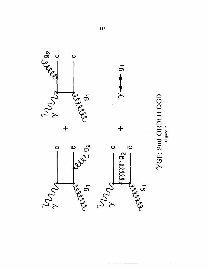
113

C\J C> (..) IC.>

T"""

C>

i r. 0

() 0 cc UJ 0

+ + cc N

0 ~ Cl

"'O i:;:

(..) IQ C\J Q IQ c

C> C\J C\J ..

C> LL. CJ r.

114

--·- ---

I :~ i ;

" ~; ..

". ;; ~, 1 .. ---.

;~:' ... ··~J.

\ \ \ \ l

...... _ \ '

" '

\

-.. ,"'·-. -- "

-... -~~-~--·r M Cl) L.. ::s en,

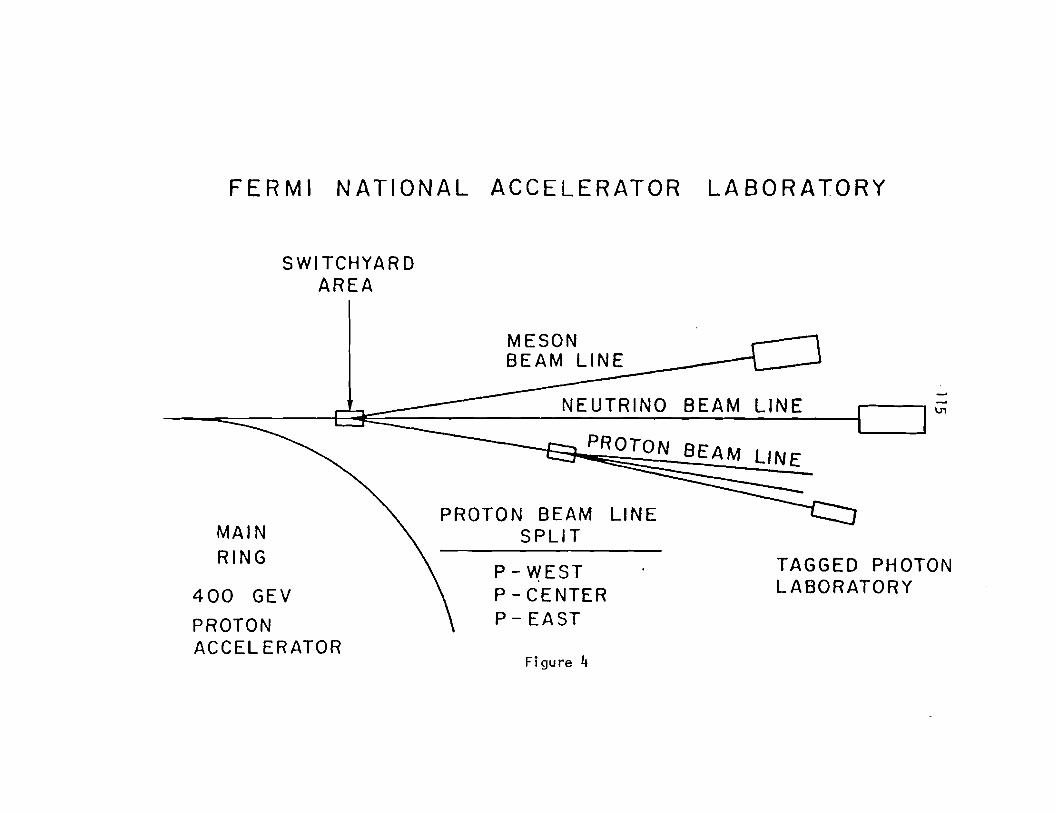
FERMI NATIONAL ACCELERATOR LABORATORY

SWITCHYARD AREA

MESON 8 EA M LINE:_------- t-_.--

~

~--o::::::-~~~~~=--~~~~~~~__..:...--=--=B~E~A~M--=L~l~N~E:__---1..-----.~

MAIN RING

400 GEV

PROTON ACCELERATOR

PROTON BEAM LINE

PROTON BEAM LINE SPLIT

P - Y{EST P-CENTER P - EAST

Figure 4

TAGGED PHOTON LABORATORY

--t-KlOO'

0 IOO' 200

I I I SCAlE I

L P-2 SERVICE BLDG

OPE RATING DURING 1976-1977 CONSTRUCTION FINISHED 1977

// / _ • / CONSlffJCTION STARTED 1917

-HGH INTENSITY PION-ANTIPROT<»I BEAM

HYPEROH ARU

\ tlGH INTENSITY LAB

\ -P-4 SERVICE BLDG '

P-3 SffMC( BLDG.

PHOTON BEAM

PHOTON LAB

EE-3 -BROAD BAND PHOTON BEAM

Figure 5

QH401H

QV400H ! BH 403 H

t ~

IT ~ v

BV 406 C TEBY

~ l V\J\/ I ,\! ~~

DUMP

TARGET BOX

BV402H

j SE 400 H BV 404 H TE BY

i i ~

[> ~ C> ~ SC 404 SC 405 (Imm) (0.5 mm)

PRE TARGET ~1

CV409C QH409C CH410C

\ I I NEUTRAL DUMP

y ·~~ ~ ~ Il 1>8 \ll\l tllB"Pb ~ 1 v

CONVET OV410C BV410C BH415H

~1 EE I

~1

Figure 6

CV423C OH423C BH4250 QV435C QH436C

\ FIE:t,0 LENS J 121121 A \7 ~i \] I> ((j~ v I ~

t t \

\ I TI~ i ~

t CH423C LT-SC425C BV426C LT-SC435C

EE4

SC 440A EXP. TARGET

D !

l t AN 440 C LT-SC4416 SC442C

>I TP 3

)Ila

Figure 7

BV437C

' C>

TP IS 2

'\]· t

BH 438 H

± 2" BEAM ENVELOPES

OH410 OH410 BH415 OH424C 8H425 OV425 8H438

1---4--~H-+-+-+-+-~----------~~~~_._,f----...._ __ ...._ __ ~~~~+-+--+-4--"--...,,._. _____ ~~*

i 211 .I'

OV409 OH436 EXPERIMENTAL TARGET

± 1"

HORIZONTAL

MOMENTUM DISPERSED FOCUS

Figure 8

120

ELECTRON BEAM YIELD PER INCIDENT PROTON

10- 5 .---~~~--..:-~~~~~~~~~--.

> CV

(.!)

0 0 v 10- 6

I­~

0 -' w 10-7

>-

10- 8 ...._~~~~---~~~~----~~~~---o 100 200 300

ELECTRON ENERGY (GeV)

Figure 9

121

01, 02

A9

A 7, A.,..;-;::;.6_..,_~

Figure 10

CONCRETE SHIELDING

TAGGING MAGNETS

0 0 0 ~

0 0 0 rt')

122

0 0 0 C\J

0 0 0

0 <D

0 ~

0 C\J

0 0

0 co

0 ta

-> QJ

(.!) ->-(.!)

0:: w z w z 0 i-0 J: a..

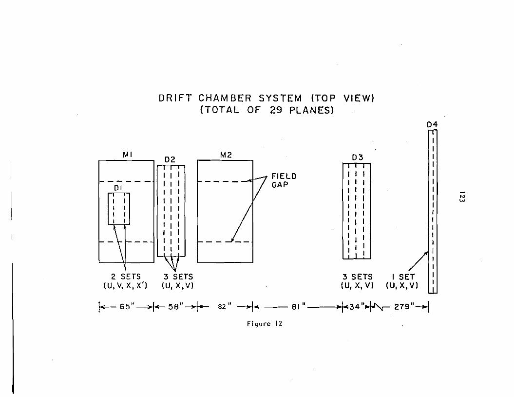
DRIFT CHAMBER SYSTEM (TOP VIEW) (TOTAL OF 29 PLANES)

Ml 02

I I ----- I I DI I I I I I I I I I I I I I I I l

2 SETS 3 SETS (U,V,X,X') (U,X,V)

M2

FIELD GAP

03

I I I I I I I I

I I I I

3 SETS (U, X, V)

04

~ 6511 >I< se" >I< 02" _,,*"'le--- a1 "--_,,•..,l'4tc34 "~ 219"~

Figure 12

-N w

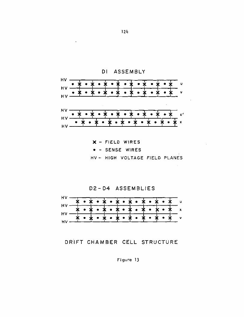
124

DI ASSEMBLY

u

v

HV • * • * • * • * • * • * • * • * x'

:~ . * . * . * . * . * . * . * . * x

X - FIELD WIRES

• - SENSE WIRES

HV - HIGH VOLTAGE FIELD PLANES

D2- D4 ASSEMBLIES

HV----r----"'T"'-----.----"'T"'-----r-----.-----.-~-.--

u HV----+------+-------~------+------------------

x HV----+-----+-----+-----+-----+-----+-----+-----+--

v

DRIFT CHAMBER CELL STRUCTURE

Figure 13

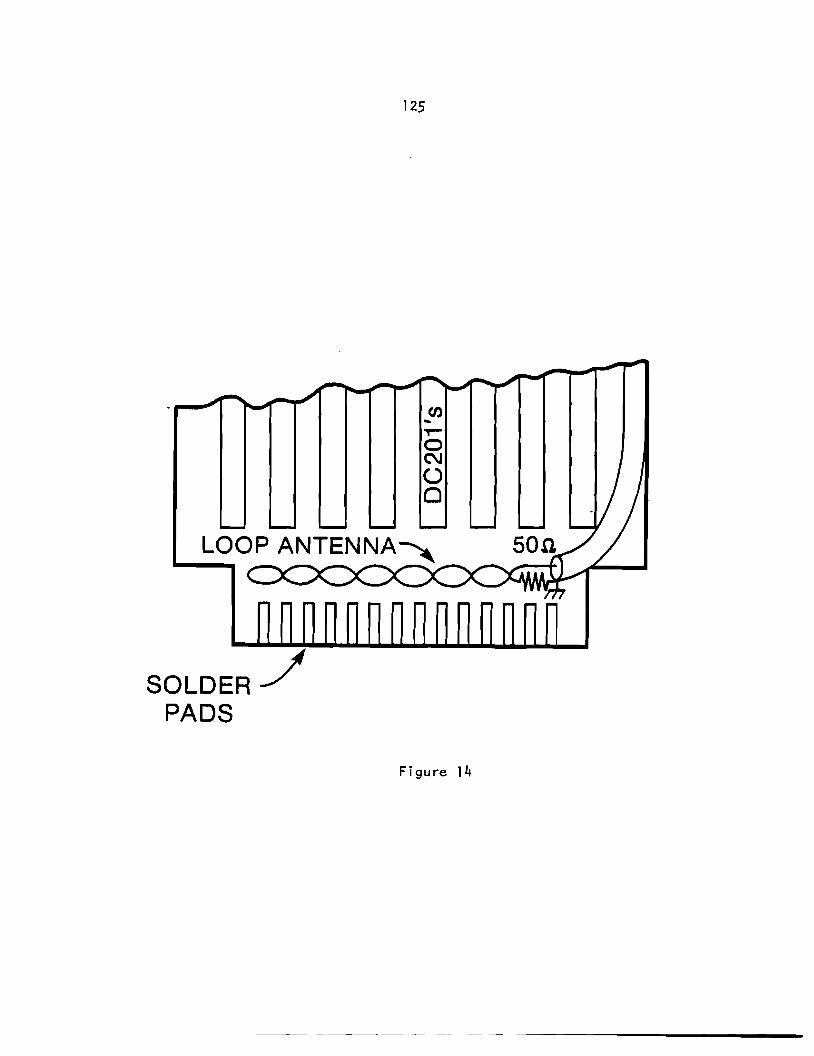
125

-r-' 0 C\J (.) Q

LOOP ANTENNA~

SOLDER_/ PADS

Figure 14

--------- -- -- - - ---------

TO PULSE GENERATOR

TO AMP. CARD

~

SECONDARY WINDINGS

(TYP.)

3E2A FERRITE TOROIDAL CORE

RGl74 50.0. CABLE

DRIFT CHAMBER INDUCTIVE PULSE SPLITTER (CUTAWAY VIEW)

PRIMARY WINDINGS

Figure 15

PC l===~~-BOARD

TO AMP.

~

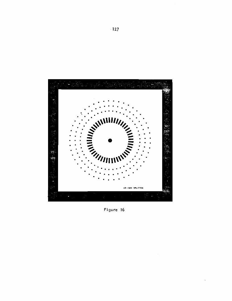
127

• • • • • • • • • • • • • • • ••• • • • • • • . ~,,,,.,,,,~ . • • • • • * ~

• • • • • ~ ~ • • • -- -- • • - • -- - • -- -- • ~ ;::: • • ~ ~ •

~,,,,,,,,,,~ • • • • • • • • • • • • • • • • •

• • • • • • • • • • •

Figure 16

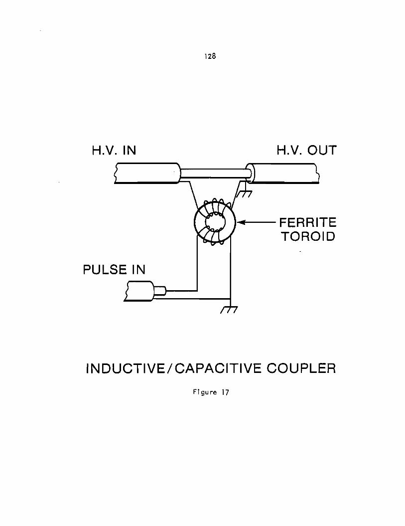
128

H.V. IN H.V. OUT

·~-FERRITE

TOROID

PULSE IN

INDUCTIVE/CAPACITIVE COUPLER

Figure 17

---- I-

- I -0 .._ 56 , ... .> J'

o:L. 0----~ ----DDRESS IN A

Jl__r """' 6 J, L-

STROBE IN

ADDRESSED ENABLE LINES (64)7

r x r I --- 2 - ... I L

J r

J -

It- ,..... r- 3

I ... r-I

. K -

I-

, ... -- 4 , .......

K . I-

I-

\ 5 K -

STROBE .....

I-I-

K FANO~ _n_ -,___ lS ~ ¥ r 7 t j

' ~

-.- +20 SP IOK~

• JHo

Gaop

LITTER UT PUT (TYP) +5-.-• .>

IOK:• 't-1 I 6S0p

H v OUTPUT

(TYP)

., .. +30 r- .> r-- IOK·~ • I ,._

J I I r

- .01 M

-f-

I,. 1,, .. >-~

I~

..

At

D4 OUTPUT

5t.AU TO R XFM

-;{, 8

SYNCH OUT

DRIFT CHAMBER TEST PULSER Figure I

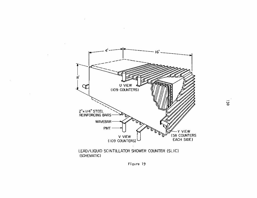
U VIEW ( 109 COUNTERS)

" ...... ..... ......................

..... 2

11x 1/4

11 STEEL '-....

REINFORCING BARS '

WAVEBAR--+<

PMT--

V VIEW ( I 09 COUNTERS)

-161 ------......1

Y VIEW ( 58 COUNTERS EACH SIDE)

LEAD/LIQUID SCINTILLATOR SHOWER COUNTER (SLIC) (SCHEMATIC)

Figure 19

CD ::? 8 w a:: 3:

13 t

0 N

Q) I... :::l Ol

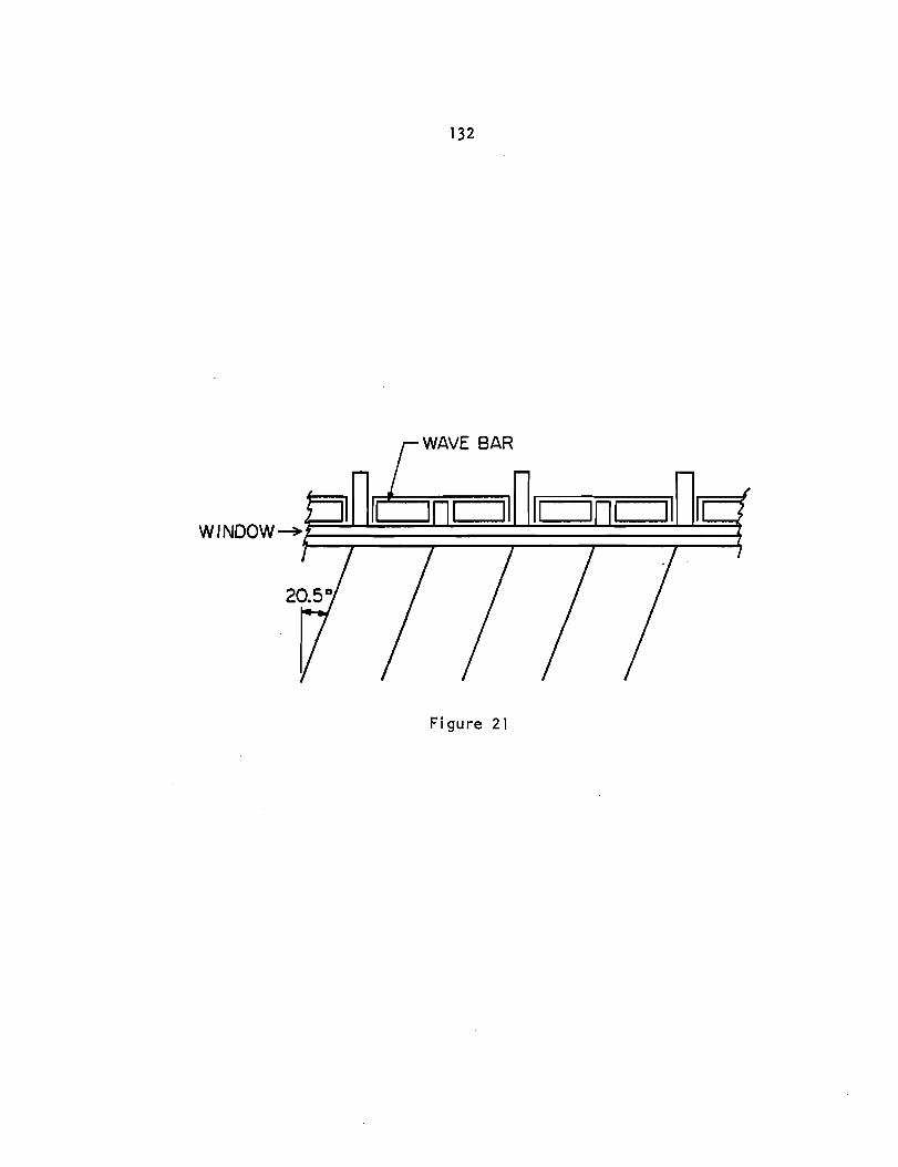
132

Figure 21

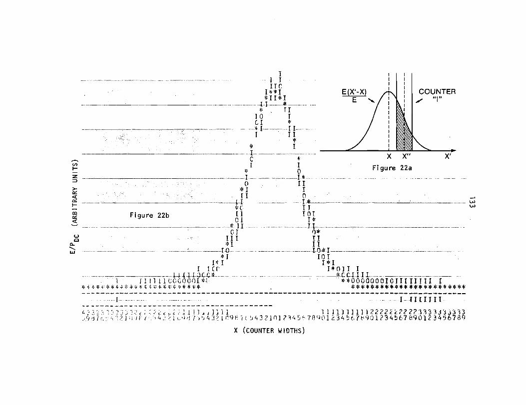
---------·--------(/) I-

I . l J II r,

I**I *H*I

-·-·--·-- ----------1-l----·-*------- ---* , TI

I 0 T CI *

--- ·- ·· ·---· ~ · !:--------- I I-- -- - -I II

* * I -~--'---------~--- --· - I---··---···-·----·- .. ··-

C * I I * 0

E(X'-X) E

---·----·····-·I -·- --- ----- ---l * ---- ·- --... -. ------ --0 . I I

* 1 I f I 0

~~~-~-----+I---------------l~

*C IT 00 Figure22b II TOT ~ 0 I I*

COUNTER ul"

x X" X' Figure 22a

........ -·-. -· -----------···-·--------------- --· --· :t. J] ... -------- ·-·--- -·- . l-t-------·----..,--·-··--·------··-----·---·--· -·-·----------. CJ Ot

g III TI a.. *l It ~ ---- --~------~----- ----·-------·--·------·---I .0.--- -- - --· -- ----------·---· ---- ------ -I-0 .t !------------··-----------·---- . --- -

*I IO I I*I I*I

I ICC' J>!IOJI I ...... --·-····~---~------------l--1.-I-W-;;iU.L---··· -- --- ... -· -- --- -- ----- ---- -~CCl-1-11------. ----·-·-·------- --

1 JlllllCOGOOOI*l **OOOOOOOIOfIIlIIII I *•*•~··········~···*····· ************************ --------------------------------------------------------------------------------

... -··---I-·-··-·-··--- I-IIlilII---·

X (COUNTER WIDTHS)

TAGGED PHOTON LABORATORY

DI INSIDE APERTURE OF Ml

C-COUNTER

OUTRIGGERS

RECOIL

TAGGING SYSTEM

LOWER LEVEL- DETECTORS

)o z BEAM DIRECTION

' I

llillllil

Figure 23

SLIC

ACCESS TO LOWER LEVEL - BELOW GROUND

HAO.

BEAM LINE

UPPER LEVEL­COUNTING ROOM

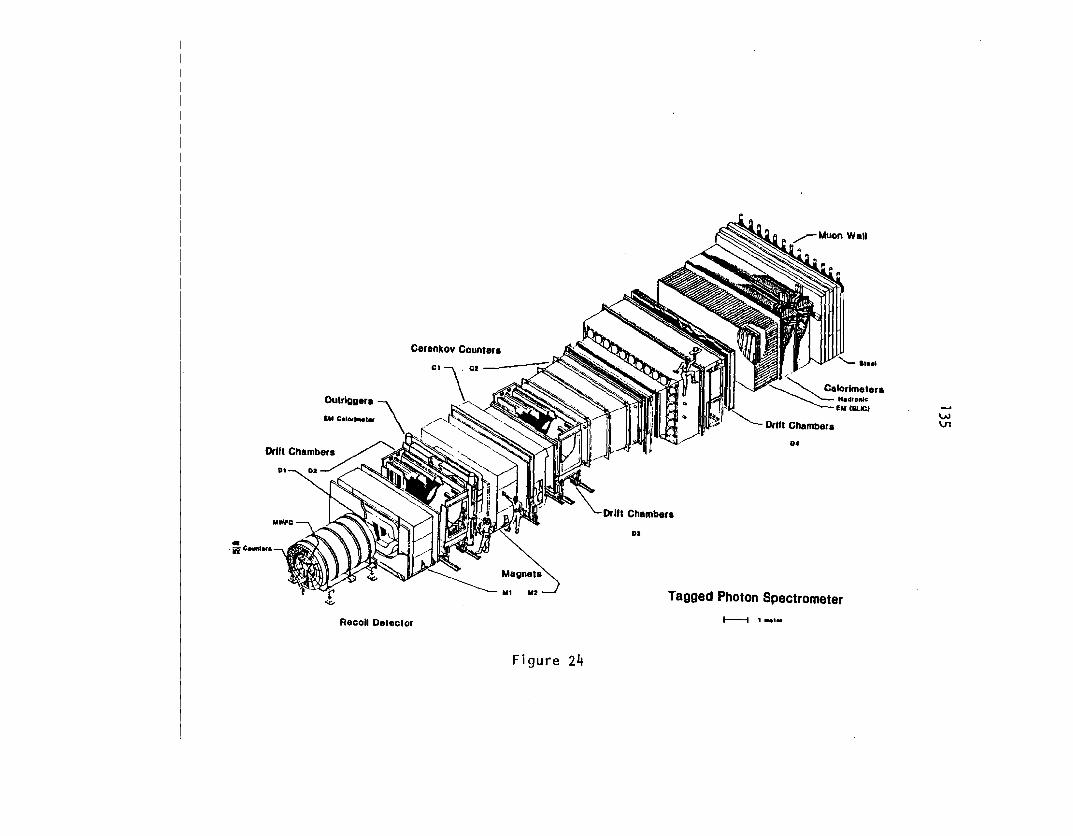
• ·iic ..... .,,

Cerenkov C ountera

Cl\

Recoil Detector

DI

Figure 24

'-•···· ·) ~lorlmetera

'-.... ~HedrOfllc ;; .......__ EU ISLICI

Drift Chamb era

Tagged Photon S pectromete 1------i r , ......

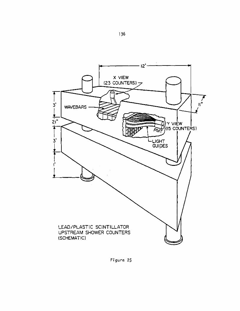
136

X VIEW (23 COUNTERS)

r 3' WAVEBARS

L 21

11

r 3'

t-,.

~

LEAD/PLASTIC SC INTI LLATOR UPSTREAM SHOWER COUNTERS (SCHEMATIC)

Figure 25

LIGHT GULDES

11"

LIQUID SCINTILLATOR CONTAINER (2 LAYERS)

PROPORTIONAL WIRE CHAMBERS

RECOIL SPECTROMETER

Figure 26

ELECTRONICS RACK

w ........

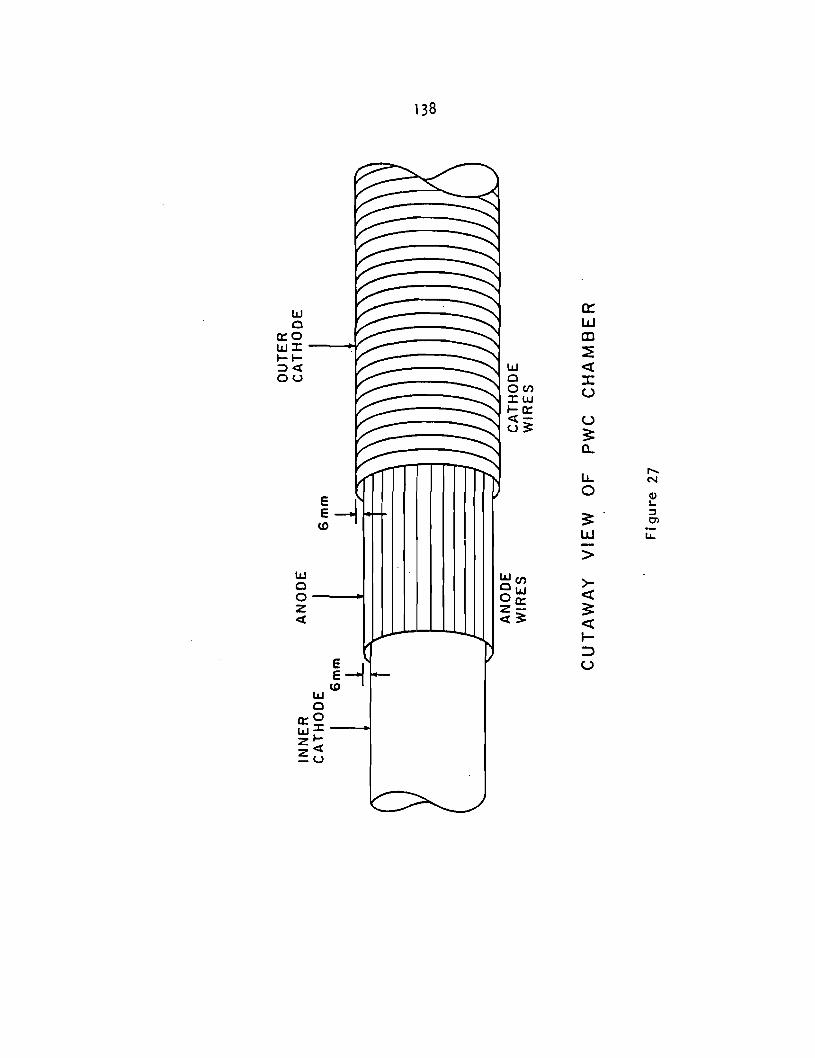
138

w 0:: 0 w

a::o CD ~

I.LI :::r::: 1-1-:::) <( I.LI <{

0 :c OU Oen u :::r::: I.LI I- a:: <(- u u3:

~ Cl.

,...... lJ.. N

0 Q) I..

~~ ::I ~ Ol

LLJ LL. c.o

-> I.LI Wen >-Ow <{ 0

Oa:: 0 z- ~ z <( 3: <{ <(

..... ::> u

~-I c.o I.LI 0

a::O I.LI :I: zl-z<r -U

T Gmm

Gmm

RECOIL PROTON TRACK

OUTER CATHODE

·(WIRES STRETCHED) TRANSVERSELY

ANODE

(WIRES STRETCHED) LONGITUDINALLY

_l_ ~~~--¥-~~~~~~~~____:..~~~~~~~ INNER CATHODE (MYLAR)

PWC CHAMBER LONGITUDINAL CROSS SECTION

Figure 28

1~

\ \

'

140

'

3: >­~ o >Z o<t wx 0 zzw <( <( z a.. <( X LL ...J w oa..

\ \

\

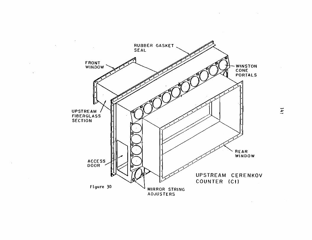
FRONT WINDOW

UPSTREAM FIBERGLASS SECTION

ACCESS DOOR

Figure 30

RUBBER SEAL

MIRROR STRING ADJUSTERS

REAR WINDOW

UPSTREAM CERENKOV COUNTER (Cl)

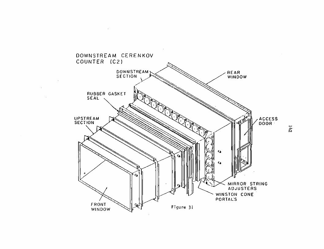
DOWNSTREAM CERENKOV COUNTER (C2)

DOWNSTREAM

SECTIO~y

RUBBER GASKET SEAL

FRONT WINDOW Figure 31

REAR WINDOW

ACCESS DOOR·

MIRROR STRING ADJUSTERS

WINSTON CONE PORTALS

Cl OPTICS

C2 OPTICS

WINSTON CONE

143

SECONDARY MIRROR PLANE

Figure 32

PRIMARY MIRROR PLANE

MIRROR PLANE

144

CERENKOV MIRROR SEGMENTATION

I I I I I I I I I I

I I I ' I I ' I

I I I I I I I I

CERENKOV MIRROR SUSPENSION

GUIDE LINES - TENSION

ADJUSTABLE FROM OUTSIDE

\ \

\ \

\ \

\ \

\ I \ I ...

Figure 33

DACRON STRINGS

4-BACK :3-FRONT

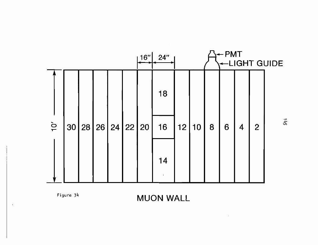
UIDE 1.16+ 24" ·I .-PMT -+-LIGHT G

18

.. 0 ,- 30 28 26 24 22 20 16 12 10 8 6 4 2

14

Figure 34 MUON WALL

UPSTREAM SLIC

SLIC

HAOROMETER

TAG-NO BUSY

TAG

Figure 35

HADRON IC TRIGGER

c

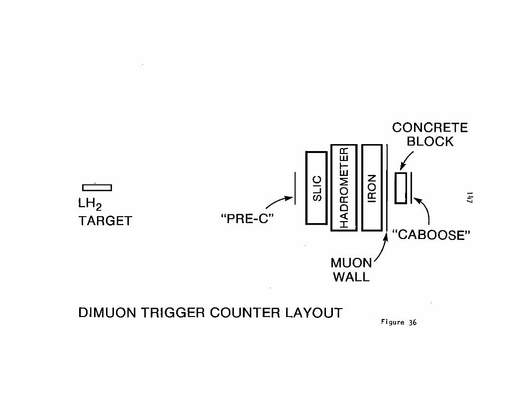
LH2 TARGET

~ "PRE-C"

(.)

.....J CJ)

a: w 1-w z ~ 0 0 a: a: 0 <( I

CONCRETE BLOCK

(

MUON

) "CABOOSE"

WALL

DIMUON TRIGGER COUNTER LAYOUT Figure 36

14

16

18

148

Pre-C Caboose

Figure 37

DI MUON TRIGGER

LOGIC

TO HADRON FAN-IN

149

ON - LINE COM PUT ER CONFIGURATION

INTERACTIVE TERMINALS

I I I I I I r---

TO CAMAC

BRANCH DRIVERS

BRANCH HIGHWAYS

HIGH LEVEL TRIGGER LOGIC -----,

DATA ACQUISITION

TASK

PDP 11155

I I I I

I I I

__ _J

1 BULK MEMORY I I I __ -- - - -----....J

Figure 38

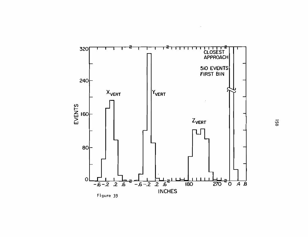
320 l I 1l211111 11111111~ CLOSEST APPROACH

510 EVENTS FIRST BIN

240

XvERT YvERT

(/) r-~ 160 > ZvERT -w \.n

0

80

-.6 -.2 .2 180

Figure 39

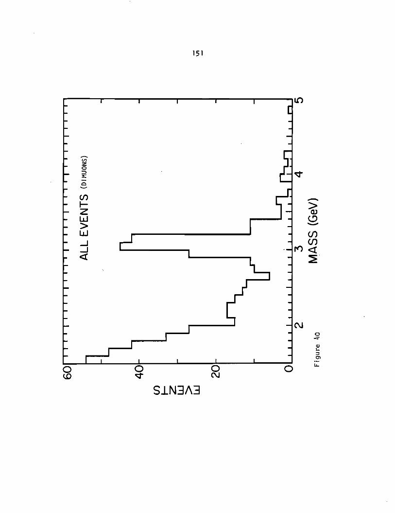
0 <.O

-V'l z 0 :;, x: -Q -

Cf) I-z w > w .....J .....J <{

0 ~

151

SJ.N3A3

0 N

0

l()

-> Q)

<..? -(/) (/)

rt') <t ~·

C\J

·-LL.

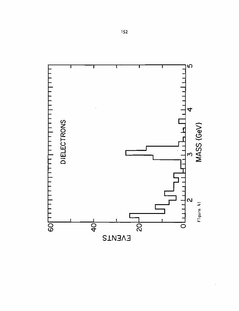
0 <.D

(J) z 0 a:: I-(.) w _J w -Cl

0 ¢

152

S!N3/\3

0 C\J

-> Q) (.? -Cf) Cf)

I") <t ~

C\J

0

0 lD

0 n:: <(

~ n:: 0 lJ..

(..)

t-Cf) <( .....J w

0 tj"

153

S1N3A3

0 N

0

lO

rt')

N

-> <1.> (.!) -(/) (/) <(

~

N ~

(I) I... ::J O'l

LL.

154

----------------------------..,...------,LO

0 U)

Q a::

~ er 0 lJ..

u -I-­Cf) <{ _J w z

0 ~

SlN3/\3

0 N

N

0

-~ (.!) -

Cf)

l--

155

(a)

8 Z FORWARD RAW

6

4

2

Q -ot--~~~~~---~_._..__~------1 > w 8

6

4

2

(b)

Z FORWARD CORRECTED

Figure 44 0.2 0.4 0.6

z 0.8 1.0

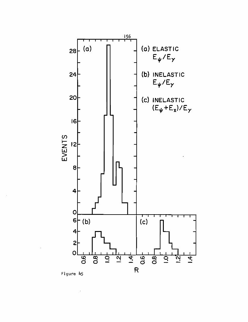
156

28 (a) (a) ELASTIC

Et/t!Ey

24 (b) INELASTIC

Et/t!Ey

20 (c) INELASTIC

(Et/t+Ex)IEy

16

en I- 12 z w > w

8

4

0 6 (b) (c)

4

2

0 w co ~ w

~ v. d d - d

Figure 45 R

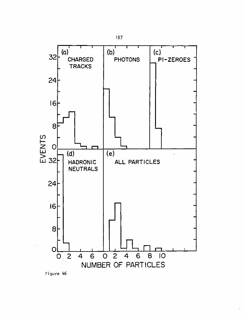
(/) 1-

(a) 32 CHARGED

TRACKS

24

16

8

157

(b) PHOTONS

(c) Pl-ZEROES

z 0~~~~--i--~--~----.__---~~-----i w ~ 32

(d) (e)

HADRONIC ALL PARTICLES NEUTRALS

24

16

8

OL--...1...---L-----L.-----J~...L---'-__._~L-.I-_.__--"-____.____.

0 2 4 6 0 2 4 6 8 10 NUMBER OF PARTICLES

Figure 46

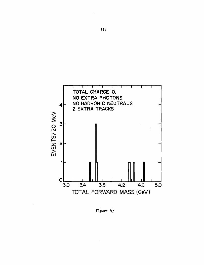
158

TOTAL CHARGE 0. NO EXTRA PHOTONS

4 NO HADRONIC NEUTRALS. 2 EXTRA TRACKS

> Q)

~

0 3 N ......... en ~ 2 w > w

O...__..__-._.. ...... _._~...__._ ............ ...._ ............ --..___. 3.0 3.4 3.8 4.2 4.6 5.0

TOTAL FORWARD MASS (GeV)

Figure 47

0.32

0.24

-.=. 0.16 \IJ

0.08

159

ELASTIC EFFICIENCY

Q.___.__.......__.____..~~---_,_------.___.

0

Figure 48

100 k(GeV)

200

-> C1'

(.!) -A

a..-i v

2

0.2

Figure 49

160

Ey= 100 GeV

0.4 0.6 0.8 1.0

z

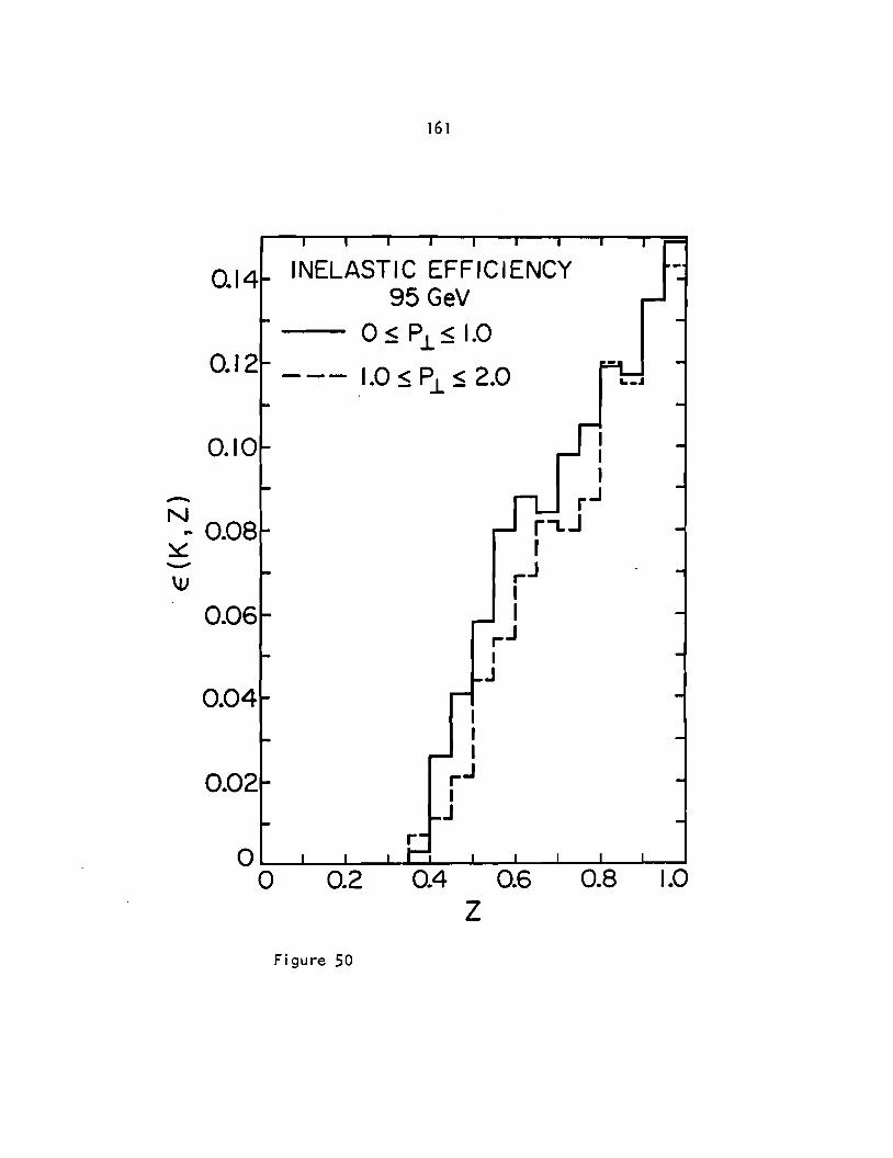
0.14

161

INELASTIC EFFICIENCY 95GeV

0 s Pi.< 1.0

O.l 2 --- 1.0 s P.i < 2.0 &. • .I

0.10

-N.. 0.08 ~ -

0.06

0.04

0.02

0.2

Figure 50

I I I

,.J I

J r

0.4 z

I I I

r.J r,_J I

.-J I I

,J I

J

0.6 0.8 1.0

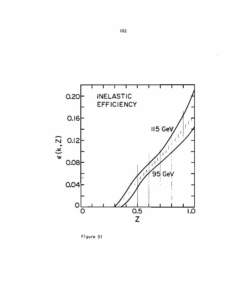
162

0.20 INELASTIC EFFICIENCY

0.16

-N 0.12 .. ~ -\IJ

0.08

0.04

Figure 51

0.5 z

1.0

0 w 1-u w a::

60

163

--CORRECTED DATA

----ESTIMATED "1' 1J CONTRIBUTION

~ 40 u Cf) 1-z w > w

trfif, r J I

I l

20

I I I I I

rtJ L OL.--L----L-----1~ ............. --'----'-~"'--........_ __ ~

0

Figure 52

0.2 0.4 0.6 0.8 Z CORRECTED

1.0

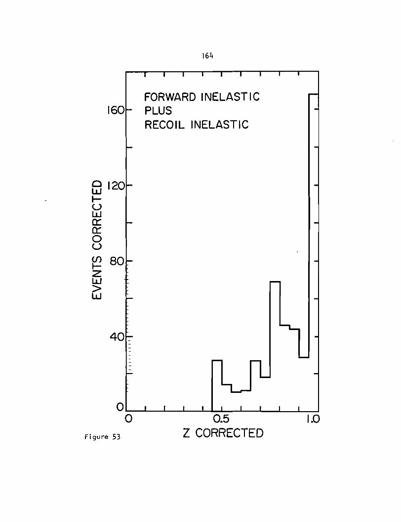
164

FORWARD INELASTIC 160 PLUS

8 120 t-u w 0::: 0::: 0 u en 80 t-z w > w

40_

Figure 53

RECOIL INELASTIC

0.5 Z CORRECTED

1.0

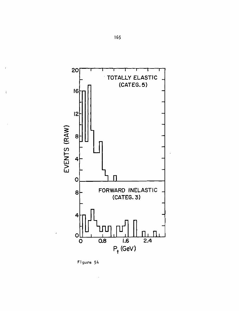
-3: <{ a:: -(/)

I-z w > w

20

16

12

8

4

0

8

4

165

. TOTALLY ELASTIC (CATEG. 5)

FORWARD INELASTIC (CATEG. 3)

O~ __ __..__._..__._. ............. ~~ ........... ~ 0 0.8 1.6 2.4

Pt (GeV)

Figure 54

166

APPENDIX ~ - TABLE§

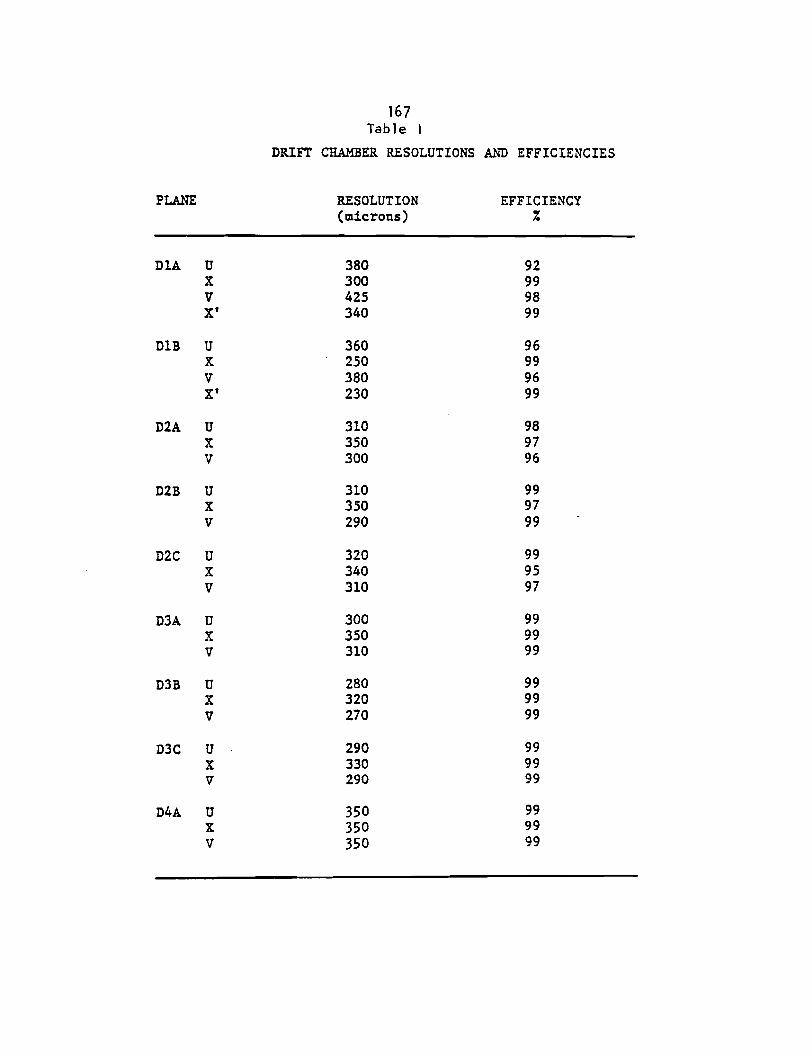
167 Tab le I

DRIFT CHAMBER RESOLUTIONS AND EFFICIENCIES

PLANE RESOLUTION EFFICIENCY (microns) %

DlA u 380 92 x 300 99 v 425 98 X' 340 99

DlB u 360 96 x 250 99 v 380 96 X' 230 99

D2A u 310 98 x 350 97 v 300 96

D2B u 310 99 x 350 97 v 290 99

D2C u 320 99 x 340 95 v 310 97

D3A u 300 99 x 350 99 v 310 99

D3B u 280 99 x 320 99 v 270 99

D3C u 290 99 x 330 99 v 290 99

D4A u 350 99 x 350 99 v 350 99

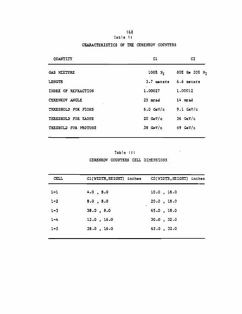
168 Tab le 11

CHARACTERISTICS OF THE CERENKOV COUNTERS

QUANTITY Cl

GAS MIXTURE 100% N2

LENGTH 3.7 meters

INDEX OF REFRACTION l.00027

CERENKOV ANGLE 25 mrad

TRRESROLD FOR PIONS 6.0 GeV/c.

THRESHOLD FOR KA.CNS 20 GeV/c.

THESHOLD FOR PROTONS 38 GeV/c.

Table 111

CERENKOV COUNTERS CELL DL"!ENSIONS

C2

80% He 207. N2

6.6 meters

1.00012

14 :nrad

9.1 GeV/c.

36 GeV/c.

69 GeV/c.

CE!.L Cl(WIDTR,HEIGHT) inc.hes C2(WIDTR,HEIGRT) inc.hes

1-1 4.0 8.0 10.0 ' 18.0

1-2 a.a t 8.a 20.0 18 .o

1-3 38.0 t a.a 65.0 , 18.0

1-4 12.0 ' 16.0 30.0 32.0

1-5 38.0 , 16.0 65.0 32.0

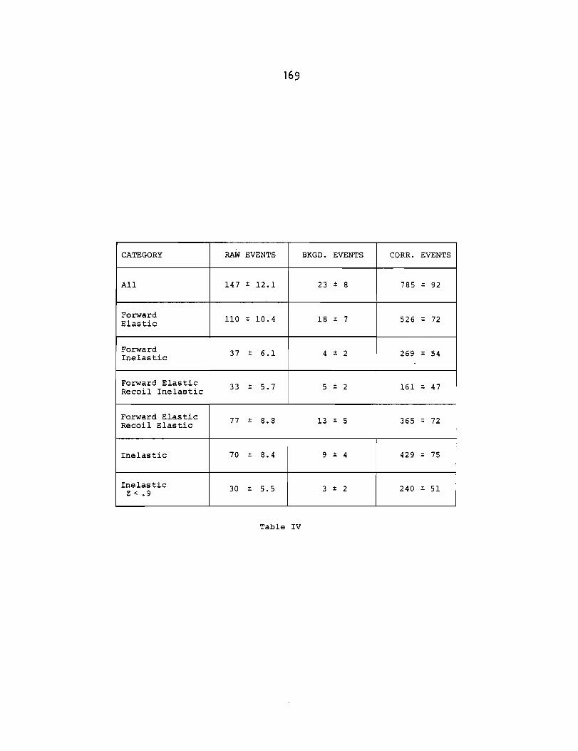
169

CATEGORY RAW EVENTS BKGD. EVENTS CORR. EVENTS

All 147 ± 12.l 23 ± a 7a5 = 92

Forward 110 = 10.4 la = 7 526 72 Elastic -

Forward 37 ± 6.1 4 ± 2 269 = 54 Inelastic

Forward Elastic 33 .!: 5.7 5 ± 2 161 47 Recoil Inelastic -

I Forward Elastic 77 :!: a.a 13 :!: 5 365 = 72 I Recoil Elastic

I I

i Inelastic 70 = a.4 9 ± 4 429 = 75 I

I

! '

Inelastic 30 ± 5.5 3 z < • 9 .!: 2 240 = 51

I

Table IV

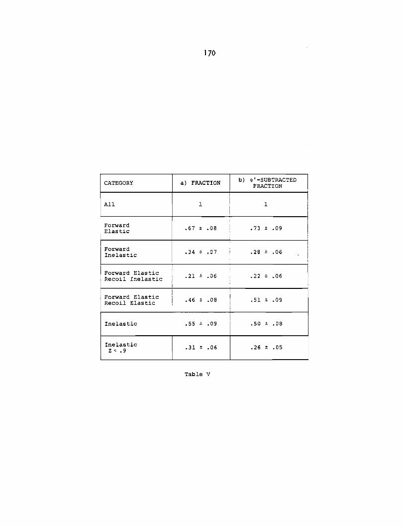
170

a) FRACTION b) 1jJ'-SUBTRACTED CATEGORY FRACTION

All 1 1

Forward .67 ± .OS .73 ± .09 Elastic

Forward .34 ± .07 .2S ± .06 Inelastic

Forward Elastic .21 ± .06 .22 ± .06 , Recoil Inelastic i ' i

Forward Elastic I .OS I • S l ± .09 I .46 ±

Recoil Elastic I ! '

I

Inelastic .SS ± .09 .so ± .OS

Inelastic .31 ± z < • 9 .06 .26 ± .as

Table V

171

CATEGORY a) CROSS SECTION(NB) b) $'-SUBTRACTED CROSS SECTION (NB)

All 21.5 ± 2.4 19.6 :!: 2.4

Forward 14.2 ± 1.9 14.2 ± 1.9 Elastic

Forward 7.3 ± 1.4 5.4 ± 1.5 Inelastic

Forward Elastic 4.4 ± 1.1 4.4 :!: 1.1 Recoil Inelastic

Forward Elastic 9.8 ± 1.8 9.8 :!: 1.8 Recoil Elastic

Inelastic 11. 7 :!: 2.0 9.8 :!: 2.1

Inelastic 6.6 ± l. 4 5.1 :!: 1.4 z < • 9

Table VI

N.B.: There is an additional ·25% uncertainty in overall normalization of cross sections.

E516 Forward Elastic

14.2:!:1.9(±3.6) @ 103 GeV

E516 z < .9

5.1±1.4(±1.3) @ 103 GeV

(ijl' subtracted)

6.6 ± l.4(±1. 7) @ 103 GeV

(ijl' not subtracted)

E516 Oz< .9

aFWD Elastic

.36 ± .07 @ 103 GeV

1jl' subtracted

.46 ± .09 @ 103 GeV

1jl' not subtracted

172

BFP(l7) EMC(l6)

Elastic z 2: .95

12.8 :!: 2.0 20.7 ± 1.2(±4.1) @ 80 - 100 GeV

@ 108 GeV ll.5 :!: 2.0

BFP Z< .9

@ 100 - 120 GeV

Table VII(a) Elastic

EMC z < .95

16.8 :!: 2.9 @ 80 - 100 GeV

16.8±1.3(±2. 7)

@

@ lll GeV 28.0 ± 4.0

@ 100 - 120 GeV

Table VII(b) Inelastic

BFP az < .9

a Elastic

@

.81 :!: .08 -108 GeV

EMC az < .95

a z ~ .95

1.3 :!: .3 80 - 100

2.4 :i: .5 @ 100 - 120

Table VII (c) Elastic/Inelastic

GeV

GeV

Wide Band Cl9 l Forward Elastic

-21(:!:3) @ -100 GeV

Wide Band

----

Wide Band

----

173

REFERENCES

1> See, for example, F. Gilman, Phys. Rep. 95.

4C. < 1972>

2> T. Appelquist, R. Barnett, K. Beyond, SLAC PUB-2100 <March 1978>.

Lane, Charm and

3> D. Duke and J. Owens, PhlJS. Lett. 96~ < 1980> 184.

4) J. 377.

Leveille and T. Weiler, Phys. Lett. 86B (1979>

5) E. Berg er and 0. Jones, Phys. Rev. 023 < 1981) 1521.

6) F. Halzen, Production of Heavy Guarks, Proceedings of the XXI International Conference on High Energy Physics, Paris, 1982, p. 381.

7> L. Jones and H. Wyld, Phys. Rev. 017 (1978) 2332.

S> J. Babcock, D. Sivers, S. Wolfram, Phys. ( 1978) 162.

9) T. Weiler, Phys. Rev. Lett. 44 <1980) 304.

Rev.

10) T. 1517.

TaJ ima, T. Watanabe, Phys. Rev. 023 <1981>

11) J. 147.

Leve i 11 e, T. Weiler, Nuc. Phys. B147 (1979>

12> H. Fritzsch, Phys. Lett. 67B <1977> 217.

13) H. Fritzsch, K. Streng, PhlJs. Lett. 72B (1978) 385.

14) R. Philips, Phenomenology of New Particle Production, Proceedings of the XX International Conference on High Energy Physics, Madison, Wisconsin, 1 980' p . 14 71 .

15> M. Binkley et al., Phys. Rev. Lett. 50 <1983) 302.

16> J.J. Aubert et al., EMC, Nuc. Phys. B213 <1983> 1.

17) T. Markiewicz, Ph.D. thesis, U. C. Berkeley, 1981.

174

18> M. Binkley et al., Phys. Rev. Lett. ~8 < 1982> 73.

19) A. 197.

Clark et al., BFP, Phys. Rev. Lett. 43 < 1979)

20) J.J. Aubert et al., EMC, CERN EP/80-84, 1980.

21> M. Strovink, Review of- Multimuon Production by Muons, Proceedings of the 1981 International Symposium on Lepton and Photon Interactions at High Energies, Bonn, W. Germany, p. 594.

22) B. Knapp et a 1. ' Phys. Rev. Lett. 34 <1975) 1040.

23) T. Nash et al. I Phys. Rev. Lett. 36. (1976) 1233.

24) u. Camerini et al. ' Phys. Rev. Lett. 35. (1975) 483.

25) B. Gittleman et a 1. I Phys. Rev. Lett. 35 (1975) 1616.

26) E. Barsotti et al. ' IEEE Trans. Nuc l. Sci. NS-2~

<1979) 686.

27> J. Martin et al., Use of the ECL-CAMAC Trigger Processor System ~or Recoil Missing Mass Triggers at the Tagged Photon Spectrometer at Fermi lab, Proceedings of the Topical Conference on the Applications of Microprocessors to High-Energy Physics, CERN, 1981.

28> T. Nash, A Review of Programmable Associated with Fermilab Experiments, ibid . ._

Systems

29) R. Mount, Multimuon Production in 280 GeV µ Iron Interactions, Proceedings of the XX International Conference on High Energy Physics, Madison, Wisconsin. 1980, p. 205.

30) This technique was suggested by Dr. Univ. of Minnesota.

T. Jensen,

31> Many of the techniques used in construction of the sp 1 i tters were suggested by C. Kerns, Fermi lab.

32> Ferroxcube Corp., Elk Grove Village, Ill.

175

33) G. Hartner et al., A Recoil Proton Detector Using Cylindrical Proportional Chambers and Scintillation Counters, accepted for publication, Nucl. Inst. Meth., 1983.

34) Y. Tsai, Rev. Mod. Phys. 46 (1974> 815.

35) C. Kerns, Fermilab.

36> J. Kenney, ProJect Engineers, Arcadia, Calif.

37> V. BharadwaJ et al., Nucl. Inst. Meth. 155 <1978> 411.

38> V. BharadwaJ et al., A Large Area Liquid Scintillator Multiphoton Detector, University of California, Santa Barbara, High Energy Physics, unpublished.

39) J. J. 275.

Aubert et al., EMC, Phys. Lett. 123B C1983>

40> Stanford: ( 1983) 90.

Physics Archaeology, CERN Courier 2~.

41 > A. Duncan, Ph.D. thesis, Univ. of Colorado, 1982.

42) See also J. Appel et al., Tagged Photon Magnetic Spectrometer: Fae i 1 i ty Design Report, Fermi lab, 1977.

43> It has been pointed out by Baier and Ruckl, Bielefeld Report BI-TP81/30 < 1980), that the Berger and Jones model depends strongly on the mass of the charmed quark. A mass of 1.2 GeV gives agreement with the EMC data <16).