high-fidelity transmission simulation for hardware-in-the ... · 2.1 clutches and brakes as part of...
TRANSCRIPT

High-Fidelity Transmission Simulation for
Hardware-in-the-Loop Applications
Orang Vahid Paul Goossens
Maplesoft
615 Kumpf Drive, Waterloo, ON, Canada, N2V 1K8
[email protected] [email protected]
Abstract
Model-based development plays a central part in op-
timizing existing transmission designs and exploring
new system architectures. Design iterations and per-
formance evaluations are done through virtual proto-
types of the transmission systems, used in hardware-
in-the-loop (HiL) simulations. In this paper,
MapleSim’s Driveline Component Library is intro-
duced. The combination of this Modelica library and
Maple’s core symbolic technology, enables engi-
neers to include more detail into their models target-
ed for real-time simulation of transmission systems.
The paper also includes some results from the work
at Aisin AW in modeling transmissions and HiL test-
ing.
Keywords: Transmissions; Hardware-in-the-loop;
symbolic calculations
1 Introduction
As automotive manufacturers strive to meet and ex-
ceed performance requirements on fuel efficiency
and ride comfort, they have focused increasingly on
the transmission design as one of the key factors.
Engineers are putting tremendous effort into deter-
mining exactly how the power is lost, and what can
be done to reduce losses and improve overall fuel
efficiency. As a result, the transmission industry is
now actively involved in optimizing existing trans-
mission designs and exploring new system architec-
tures. At the same time, transmission controllers are
becoming more complicated and more detailed prod-
uct testing is needed than ever before.
Model-based development (MBD) plays a central
part towards achieving these goals. Design iterations
are done through virtual prototypes of the transmis-
sion systems, used in hardware-in-the-loop (HiL)
simulations. Virtual prototyping can yield more effi-
cient products at significantly reduced costs by al-
lowing engineers to address design issues long be-
fore they invest in physical prototypes.
In this paper we report on some of the activities
under taken at AISIN AW in Japan regarding HiL
simulation and the use of MapleSim environment to accelerate the development of automatic transmis-sions. The requirements for low calculation cost
plant models for real-time simulations were met by
creating the gear train part of the model in MapleSim. These models are then exported as opti-
mized c-code for implementation into the HiL sys-
tem.
2 Transmission Modeling Using the
Driveline Component Library
The transmission models referred to in this paper are
built using the components from the MapleSim
Driveline Component Library (DCL) [1] as well as
other components from the Standard Moldelica Li-
braries [2]. DCL covers all stages in a powertrain
model from the engine through to the differential,
wheels and road loads (See Figure 1). Furthermore,
the library allows for flexible inclusion of power loss
data that best reflect the way in which the loss data
was acquired.
In the remainder of this section, some of the fea-
tures of the components used in modeling transmis-
sions are discussed.
2.1 Clutches and Brakes
As part of the standard component library, MapleSim
provides two clutch models: a standard, controllable
friction clutch and a one-way clutch [2].
In DCL, these models are expanded; clutch and
brake models provide a real output port for the loss
power and a Boolean output port to indicate clutch
lock-up. There are also other formulation improve-
ments that make DCL models perform better when
used with fixed-step integrators usually encountered
DOI Proceedings of the 9th International Modelica Conference 907 10.3384/ecp12076907 September 3-5, 2012, Munich, Germany

in real time applications and Hardware-in-the-Loop
simulations.
Figure 1: Driveline Component Library
2.2 Torque Converter
The torque converter is modeled using tables of
measured data. The following characteristics are
used:
• Torque Ratio vs Speed Ratio
• Load Capacity vs Speed Ratio
Where subscripts “t” and “p” designate turbine and
pump quantities, respectively. The required data can
be given as tabulated data. The Torque Converter
component supports two alternative formulations
based on the following definitions of the load capaci-
ty :
Backward flow, happens during deceleration of
the vehicle where the vehicle kinetic energy is
transmitted back through the transmission to the en-
gine. In this situation, the turbine is pumping and the
pump is acting as a turbine. Since torque converters
are not designed to work optimally this way, the
torque converter will have very different characteris-
tics. This is accommodated in the lookup table data
by providing torque ratios and capacity values for
, typically up to about 5.
In the test model shown in Figure 2, the input
(pump) torque is increased linearly for the first 10
seconds. At low speeds, between t = 0 and 4 s, the
turbine torque increases faster than the input torque.
This is the “torque multiplication” effect typically
seen in the torque converters [3]. Due to the inherent
inefficiencies in the mechanism, the turbine speed is
slightly less than the pump speed while the torque is
driving the pump.
Figure 2: Torque converter test model
High-Fidelity Transmission Simulation for Hardware-in-the-Loop Applications
908 Proceedings of the 9th International Modelica Conference DOI September 3-5, 2012, Munich Germany 10.3384/ecp12076907
Note that when the input torque drops at t = 15 s,
the kinetic energy of the dynamometer changes the
torque flow from forward to backward (i.e. turbine
drives the pump), and the pump speed drops below
the turbine speed.
2.3 Gears, Gear Sets, and Transmissions
DCL includes simple and compound gear sets and
related actuation components for modeling gear
trains and transmissions (see Figure 1). The
Ravigneaux gear set component is discussed in the
following as an example of the compound gear com-
ponents in DCL.
Ravigneaux Gear Set
The Ravigneaux configuration is a basic automatic
transmission planetary assembly. As shown Figure 3,
this configuration is constructed internally using
three Planet-Planet components and one Planet-Ring
component.
Figure 3: Internal structure of the Ravigneaux
Gear
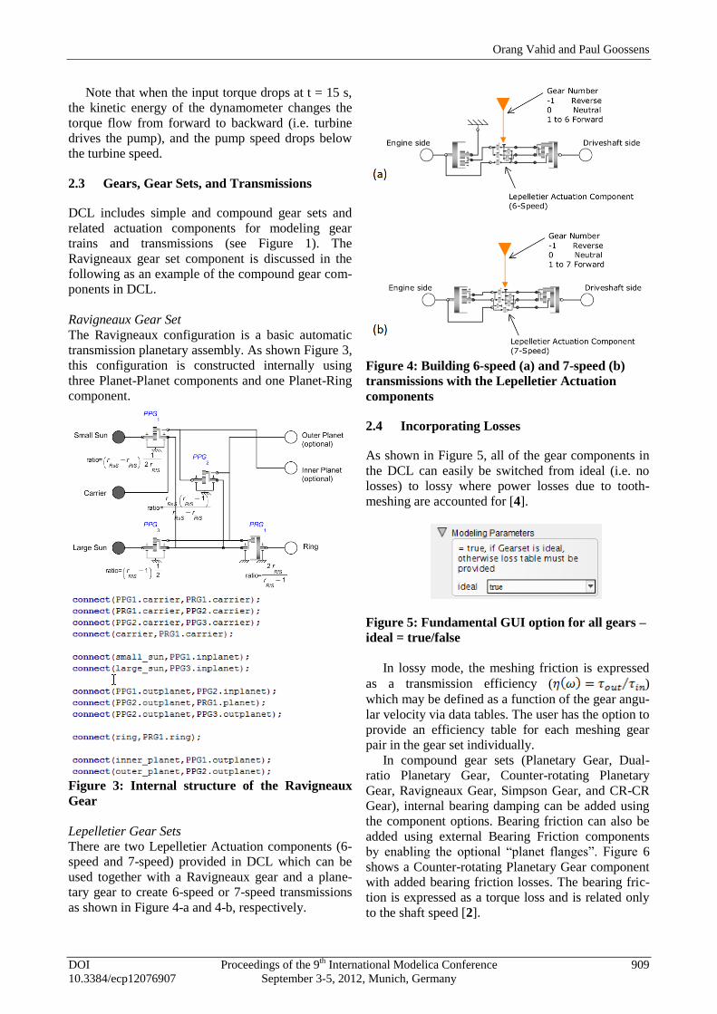
Lepelletier Gear Sets
There are two Lepelletier Actuation components (6-
speed and 7-speed) provided in DCL which can be
used together with a Ravigneaux gear and a plane-
tary gear to create 6-speed or 7-speed transmissions
as shown in Figure 4-a and 4-b, respectively.
Figure 4: Building 6-speed (a) and 7-speed (b)
transmissions with the Lepelletier Actuation
components
2.4 Incorporating Losses
As shown in Figure 5, all of the gear components in
the DCL can easily be switched from ideal (i.e. no
losses) to lossy where power losses due to tooth-
meshing are accounted for [4].
Figure 5: Fundamental GUI option for all gears –
ideal = true/false
In lossy mode, the meshing friction is expressed
as a transmission efficiency ( )
which may be defined as a function of the gear angu-
lar velocity via data tables. The user has the option to
provide an efficiency table for each meshing gear
pair in the gear set individually.
In compound gear sets (Planetary Gear, Dual-
ratio Planetary Gear, Counter-rotating Planetary
Gear, Ravigneaux Gear, Simpson Gear, and CR-CR
Gear), internal bearing damping can be added using
the component options. Bearing friction can also be
added using external Bearing Friction components
by enabling the optional “planet flanges”. Figure 6
shows a Counter-rotating Planetary Gear component
with added bearing friction losses. The bearing fric-
tion is expressed as a torque loss and is related only
to the shaft speed [2].
Orang Vahid and Paul Goossens
DOI Proceedings of the 9th International Modelica Conference 909 10.3384/ecp12076907 September 3-5, 2012, Munich, Germany

Figure 6: Adding bearing friction to gear sets
3 Advantage of the Symbolic Tech-
nology
Symbolic techniques turn out to be a critical ingredi-
ent, both to enable efficient modeling of these com-
ponents as well as to generate optimized code, yield-
ing the required HiL execution speed. MapleSim’s
symbolic capabilities are enabled by an underlying
Maple computation engine [6], providing extremely
efficient symbolic operations that are necessary for
handling the thousands of system equations typically
found in the transmission models.
A common characteristic of Modelica environ-
ments is that system models are built by assembling
components using “physical” connections, carrying
quantities like torque and rotational angle bi-
directionally between the two components. The deci-
sion on causality of the model is deferred to simula-
tion time, just before the numeric integration process
is started. This is possible because the entire set of
equations for the whole system is generated symbol-
ically, as a first step. At this point we typically have
a set of differential algebraic equations. As shown in
Figure 7, several steps are necessary before these
equations can be solved numerically, yielding simu-
lation results and/or HIL code. These steps are dis-
cussed next.
3.1 Equation Simplification
The initial set of equations generated from the sys-
tem model is typically large and contains many re-
dundancies. Symbolic techniques are used to simpli-
fy this set of equations as much as possible. The
simplifications are exact and do not result in any loss
of fidelity in the model. Trivial equations of the form
a = b are removed. Linear equations are pre-solved
analytically. Reducing the number of equations by a
factor of ten is not uncommon. This simplification
step is key to the scalability of the remaining pre-
processing steps.
Figure 7: Steps towards numerical simulation
3.2 Index Reduction
The generated system consists of differential alge-
braic equations (DAEs). Such equations cannot be
readily solved with standard numerical techniques
because of the presence of algebraic constraints. The
“index” of a DAE is loosely defined as the number
of times the equations need to be differentiated in
order to remove these constraints. The goal here is to
reduce the system of equations to “index 1”, allow-
ing numeric integration. During integration, the con-
straints are monitored for “drift”, ensuring an accu-
rate solution, reflecting the behaviour of both the
differential equations as well as algebraic con-
straints. Again, symbolic techniques turn out to be
essential, allowing differentiation of equations and
efficient index reduction.
3.3 Causalization
At this point, we have a simplified system of (index
1) differential equations. In order to numerically
solve this system, we will need to repeatedly evalu-
ate the system for a particular point. To enable this,
we will need to turn our (acausal) system of equa-
tions into a (causal) sequence of numeric operations.
In short, this process involves imposing an order of
evaluation onto our set of equations. Doing this effi-
ciently involves tools from graph theory, readily
available in the symbolic computing tool chest.
3.4 Optimized Code Generation
Executing speed is critical to HiL applications and
symbolic techniques again turn out to be key to gen-
High-Fidelity Transmission Simulation for Hardware-in-the-Loop Applications
910 Proceedings of the 9th International Modelica Conference DOI September 3-5, 2012, Munich Germany 10.3384/ecp12076907

erating highly efficient code. It is, of course, possible
to generate code directly from the causal system of
equations described above. However by looking at
those equations globally, we are able to perform
symbolic optimizations prior to generating code,
which makes the difference between achieving the
required HiL cycle times or not. These optimizations
involve detecting common computation sequences
that can be factored out, which go way beyond the
(local) optimization capabilities of available compil-
ers.
3.5 Two Examples
A Simple Driveline Model:
Consider the driveline mode shown in Figure 8.
The model represents a vehicle powertrain from en-
gine to dynamometer. The model includes a torque
converter between the flywheel and the transmission.
The transmission is a 4-speed Ravigneaux gearbox.
Using throttle and brake controllers, the speed is
changed following a ramp-up/coast down profile.
Using MapleSim’s API commands from Maple,
the simulation time is measured. A fixed time-step
solver (Euler) is used here with a time step of 0.001
sec. Total simulation time is 150 seconds. The simu-
lation was done on a 64-bit Windows 7 machine with
Intel(R) Core(TM) Duo 2.40 GHz CPU. Figure 9
shows Maple’s commands for this example. These
command extract and simplify the model
equationsand convert them to optimized c-code. The
simulation results are obtained from a Maple proce-
dure which includes the complied c-code.
Figure 8: An example of a complete powertrain.
The simulation was done over 15 times faster
than real-time (i.e. ~10 second of integration time for
a 150-second simulation). In 20 consecutive runs the
average simulation time was 9.68 with standard de-
viation of 0.30.
Figure 9: Running MapleSim simulation using
API commands in Maple
A Vehicle Model with Mean-value Engine Model:
The system in Figure 10, is the second example cho-
sen for the real-time demonstration. This model is
considerably more complex than the previous exam-
ple and includes a detailed mean-value engine model
[7] and a 4-speed transmission model. The
MapleSim model uses the New York City Cycle [8]
and runs for 600 seconds. Simulation timing was
done under similar solver settings as the previous
example. The same computer was also used. On av-
erage the simulation was done about 12 times faster
than real-time (i.e. ~50 second of integration time for
a 600-second simulation). Based on 15 consecutive
runs the average simulation time was 50.2 seconds
with standard deviation of 0.54.
4 HiL Simulation of the Automatic
Transmissions
At AISIN AW, HiL simulation is extensively used to
accelerate the development of automatic transmis-
sions. The plant models for HiL simulations require
sufficiently high fidelity to accurately represent the
aspect of the system dynamics important to the de-
signers. At the same time, these models have to have
low calculation cost in order to enable real-time exe-
cution.
As shown in Figure 11, the real-time platform used
in the HiL simulations reported here is the ADX sys-
tem [9] from A&D Technology, Inc.
The plant model is deployed in Simulink [10] and
can be separated into two parts as depicted in Figure
12. The first part is the plant model which is con-
structed of the s-function generated from MapleSim
models including clutches, brakes, and various gear
sets. This part also includes Simulink blocks for oth-
er parts of plant model. The second part is the auto-
matic testing module.
It is critical that the calculation time associated
with the first part (plant model) is kept as low as
Orang Vahid and Paul Goossens
DOI Proceedings of the 9th International Modelica Conference 911 10.3384/ecp12076907 September 3-5, 2012, Munich, Germany

possible to accommodate for the high execution
times of the increasingly more complex automatic
testing routines implemented in the testing module.
Figure 11: HiL simulation system
Figure 12: Model for Real-time system
A sample gear train is shown in Figure 13 which
includes a planetary gear, a Ravigneaux gear, and a
basic gear connected together using three clutches,
two brakes (modeled using clutch components), and
a one-way clutch. This gear train is connected to an
ideal gear which represents the differential gear ra-
tio. The tire load is modeled using additional inertia,
clutch, and brake components. The tire component
and the longitudinal vehicle dynamics component
(refer to Figure 1) are not used here since that level
of fidelity is not necessary for the intended HiL sim-
ulations.
Figure 14 shows the HiL simulation results with
s-function generated from MapleSim. Compared
with another software previously used, it was shown
that for the above model, the implementation of the
s-function generated from MapleSim in the HiL sim-
ulations with a sampling time of 1ms, reduced the
overall CPU time by 250s (or 25% of a time step).
This reduction is due to fact that the MapleSim’s s-
function runs twice as fast as the previously imple-
mented block.
5 Conclusions
In this paper some of the features of the Driveline
Component Library – an add-on Modelica library for
MapleSim modeling, simulation, and analysis envi-
ronment – were introduced. The Driveline Compo-
nent Library provides a comprehensive set of com-
ponents that enable transmission manufacturers – as
well as other automotive developers – to convenient-
ly create plant models for control and simulation.
The underlying symbolic computation engine of
MapleSim (i.e. Maple) expands the inherent ad-
vantages of similar Modelica-based physical model-
ing tools to new heights. Benefiting from the power
of symbolic computing, MapleSim can generate ex-
tremely fast code that is of vital importance when
simulating large complex systems in real-time.
Figure 10: Full vehicle model in MapleSim
High-Fidelity Transmission Simulation for Hardware-in-the-Loop Applications
912 Proceedings of the 9th International Modelica Conference DOI September 3-5, 2012, Munich Germany 10.3384/ecp12076907

Figure 13: Gear train model created in MapleSim
Figure 14: A sample of HIL simulation results
The paper also included a brief description of the
activities at AISIN AW on the development of new
automatic transmissions and their use of MapleSim
and the Driveline Component Library in HiL simula-
tions. The optimized c-code generated by MapleSim
from transmission plant models enabled AISIN AW
to perform more detailed HiL simulations. In a sam-
ple case study, it was shown that the s-function gen-
erated by MapleSim ran twice as fast as the s-
function generated by a similar tool.
References
[1] MapleSim User’s Guide, 2011, ISBN 978-1-
926902-09-8.
[2] https://www.modelica.org/ (accessed
2/4/2012).
[3] D. Hrovat and W.E. Tobler. “Bond graph
modeling and computer simulation of auto-
motive torque converters,” Journal of the
Franklin Institute. Volume 319, Issues 1-2,
January-February 1985, pp 93-114.
[4] Pelchen C., Schweiger C., and Otter M.,
“Modeling and Simulating the Efficiency of
Gearboxes and of Planetary Gearboxes,” 2nd
International Modelica Conference, Proceed-
ings, pp. 257-266.
[5] Joško Deur, Vladimir Ivanovic´, Matthew
Hancock, and Francis Assadian. "Modeling
and Analysis of Active Differential Dynam-
ics," Journal of Dynamic Systems, Measure-
ment, and Control, 2010. Volume 132 /
061501, pp 1-14.
[6] Bernadin L., Chin P., DeMarco P., Geddes
K. O., Hare D. E. G., Heal K. M., Labahn G.,
May J. P., McCarron, Monagan M. B.,
Ohashi D., and Vorkoetter S. M., Maple
Programming Guide, 2011, ISBN 1-926902-
08-1.
[7] - , “Mean-Value Internal Combustion Engine
Model”, Maplesoft, White Paper,
http://www.maplesoft.com/contact/webforms
/whitepapers/enginemodel.aspx, (accessed:
2/4/2012).
Orang Vahid and Paul Goossens
DOI Proceedings of the 9th International Modelica Conference 913 10.3384/ecp12076907 September 3-5, 2012, Munich, Germany

[8] -, Dynamometer Driver's Aid, http://www.epa.gov/nvfel/testing/dynamomet
er.htm, (accessed: 2/4/2012).
[9] http://www.aanddtech.com/ADX.html (ac-
cessed: 2/4/2012).
[10] http://www.mathworks.com/products/simulin
k/ (accessed: 2/4/2012).
High-Fidelity Transmission Simulation for Hardware-in-the-Loop Applications
914 Proceedings of the 9th International Modelica Conference DOI September 3-5, 2012, Munich Germany 10.3384/ecp12076907