high-order exponential time differencing methods … exponential time differencing methods for...

High-order Exponential Time DifferencingMethods for Solving One-dimensional Burgers’

EquationDingwen Deng∗, and Jianqiang Xie

Abstract—This paper is devoted to the development andapplication of two high-order numerical methods for solv-ing one-dimensional (1D) Burgers’ equations, which are bothfourth-order accurate in both time and space. One of them isbased on the uses of Crank-Nicolson (CN) method combinedwith Richardson extrapolation method for temporal integrationand fourth-order compact finite difference approximation forspatial discretization. Additionally, a combination of fourth-order time stepping method based on Pade approximationfor temporal discretization with fourth-order compact finitedifference method for spatial approximation yields the otherfourth-order method. Using matrix analysis methods, we studytheir stability. Numerical experiments illustrate the accuracyand efficiency of new algorithms.

Index Terms—Burgers equation; Hopf-Cole transformation;Compact finite difference scheme; Pade approximation; Stabil-ity;

I. INTRODUCTION

In this article, we consider the numerical simulationsof 1D Burgers’ equation with nonhomogeneous boundaryconditions as follows

∂u

∂t+ u

∂u

∂x= γ

∂2u

∂x2, (x, t) ∈ [a, b]× [0, T ],

u(a, t) = c, u(b, t) = d, t ∈ [0, T ],

u(x, 0) = φ(x), x ∈ [a, b],

(1)

where γ, a, b, c and d are all constants and γ is thecoefficient of kinematic viscosity. This equation was firstfound by Bateman [1] and later applied to model freeturbulence by Burgers [2], [3]. Since then, it is extensivelyreferred to as Burgers’ equation [1]–[6], which has becamea very important nonlinear evolution equation because of itsimportance in various fields such as gas and fluid dynamics,traffic flow, heat conduction, wave propagation in acousticsand hydrodynamics, etc. Consequently, considerable atten-tion has been paid on the study of Burgers equation. Forexample, using Hopf-Cole transformation, we can obtainexact solutions in terms of infinite Fourier series for giveninitial condition, which fail to converge for relatively smallγ, such as γ < 0.01. Moreover, several classes of special

Manuscript received October 25, 2015; revised January 12, 2016. Thiswork is partially supported by the National Natural Science Foundationof China (Grant Nos. 11401294, 11326046, 11261040), Youth NaturalScience Foundation of Jiangxi Provincial Education Department (Grant No.GJJ14545) and Youth Natural Science Foundation of Jiangxi province (GrantNo. 20142BAB211003).

Dingwen Deng is with the College of Mathematics and InformationScience, Nanchang Hangkong University, Nanchang 330063, China (Corre-sponding Author, e-mail: [email protected])

Jianqiang Xie is with the College of Mathematics and InformationScience, Nanchang Hangkong University, Nanchang 330063, China

analytic solutions can also be obtained by using homotopyperturbation method and differential transformation method[7] and tanh function expansion method [8], etc. However, itis very difficult to find the useful expression of exact solutionto Burgers with arbitrary initial and boundary conditions.Thus, over the years, numerical studies for initial-boundaryvalue problem (IBVP) (1) have attracted widespread atten-tion. Many numerical methods including finite differencemethods (FDMs) [9]–[15], finite element methods (FEMs)[16], [17], local discontinuous Galerkin methods [18], [19],spectral methods [20], [21], collocation method based on theLaplace transform [22], meshless approach [23] and differen-tial quadrature methods [24], [25] have been developed andapplied to solve IBVP (1).

Recently, high-order compact (HOC) FDMs, which havebeen widely used to deal with various computational prob-lems arising from a wide range of applied fields due to theirhigh accuracy, compactness and better resolution for high-frequency waves [26]–[29], have been proposed for solvingBurgers equation. For example, a HOC FDM, which issecond-order temporally accurate and fourth-order spatiallyaccurate, has been developed in [9]. A sixth-order com-pact FDM combined with explicit third-order total variationdiminishing (TVD) Runge-Kutta method (RKM) has alsobeen developed in [13]. They were both directly constructedfor IBVP (1) without the use of Hopf-Cole transformation.Whereas, another two HOC FDMs were established for lineardiffusion equation obtained using Hopf-Cole transformationto Burgers equation in [11], [14], respectively. HOC methodsstated above have been limited to the use of small timesteps due to low-order accuracy in time, or strong stabilityrestriction. Besides, low-order accuracy at boundary resultsin the increase of global error. For example, in the caseof nonhomogeneous boundary, HOC FDM in [14] has onlysecond-order accuracy at boundary, thus reducing resolutionof numerical solutions.

Recently, a class of combined schemes, which consist ofhigh-order time stepping methods based on Pade approxima-tions and second-order centered difference for spatial vari-able, have been derived for linear diffusion equation obtainedusing Hopf-Cole transformation to Burger’s equation (see[15]). Although they are high-order accurate in time andunconditionally stable, they have only second-order accuracyin space. Therefore, they may generate numerical solutionof poor quality if the spatial mesh is not refined sufficiently.However, mesh refinement may lead to a large number ofarithmetic operations.

More recently, a unconditionally stable fourth-order nu-merical method, which combines fourth-order time stepping

IAENG International Journal of Computer Science, 43:2, IJCS_43_2_04

(Advance online publication: 18 May 2016)

______________________________________________________________________________________

methods based on Pade approximations with fourth-ordercompact FDM for spatial variable, have been proposed forconvection-diffusion equation [30]. Numerical results testifyhigh-performance and usefulness of that algorithm.

In this paper, enlightened by the work of [30], we derivetwo fourth-order numerical methods for Burgers equation.First, IBVP (1) is transformed into a linear diffusion equationwith mixed boundary conditions by using the Hopf-Coletransformation. Secondly, a compact FDM which has fourth-order accuracy at both interior and boundary points hasbeen derived for linearized equation, thus resulting in aninitial value problem (IVP), which can be solved exactlyusing Duhamel’s principle. Thirdly, using [1,1]-Pade to ap-proximate matrix exponential function results in a second-order CN scheme, which can be improved to fourth-orderaccuracy in time by Richardson extrapolation method and theapplication of [2,2]-Pade approximation to matrix exponen-tial function generates a fourth-order time-stepping scheme.Finally, the use of Simpson’s integrable formula to Hopf-Cole transformation in subinterval [xj−1, xj+1] (see Section2) yields fourth-order approximate solution of IBVP (1)according to fourth-order numerical solution of linearizedequation. The new methods overcome some deficiencies ofthose algorithms proposed in [9], [11], [13]–[15].

This paper is organized as follows. Construction andstability analysis of numerical algorithms are studied forIBVP (1) in Section 2 and Section 3, respectively. In Section4, five examples are carried out to test the performance ofour algorithms. Final section focuses on concluding remarks.

II. FOURTH-ORDER NUMERICAL METHODS

This section concentrates on the derivation of new numer-ical methods.

A. Notations and auxiliary Lemmas

∆t = T/K, tk = k∆t, 0 ≤ k ≤ K. Moreover, h =(b − a)/n represents grid spacing. The spatial grid nodesxj = a + jh, j = 0, 1, . . . , n form the following sets Ωh =xj |0 ≤ j ≤ n. On Ωh, we define grid function spaceSh = w|(w0, w1, . . . , wn−1, wn)T and introduce centereddifference operator δ2

xwj = (wj+1 − 2wj + wj−1)/h2. Tomake this paper self-contained, we first give two lemmasused later.Lemma 1 (cf. [30]) Assume that w(x) ∈ C5[a, b], then

w′(x0) =

w(x1)− w(x0)h

− 5h

12w′′(x0)

− h

12w′′(x1)− h2

12w(3)(x0) +O(h4),

w′(xn) =

w(xn)− w(xn−1)h

+5h

12w′′(xn)

+h

12w′′(xn−1)− h2

12w(3)(xn) +O(h4).

Lemma 2 (cf [30]) If ∀ z ∈ C and has non-positive realpart, then the following inequalities

∣∣∣2 + z

2− z

∣∣∣ ≤ 1,

∣∣∣∣1 + z/2 + z2/121− z/2 + z2/12

∣∣∣∣ ≤ 1

hold.

III. ESTABLISHMENT OF NUMERICAL METHOD

Applying Hopf-Cole transformation to the Burgers’ Eq.(1):

u(x, t) = −2γvx(x, t)v(x, t)

, (2)

Eq. (1) can be rewritten equivalently as

∂v

∂t= γ

∂2v

∂x2, (x, t) ∈ (a, b)× [0, T ],

2γvx(a, t) + cv(a, t) = 0,

2γvx(b, t) + dv(b, t) = 0, t ∈ [0, T ],

v(x, 0) = exp−

∫ x

a

φ(s)2γ

ds

, a ≤ x ≤ b,

(3)

In this paper, Vj(t) and V kj denote the approximations to

v(xj , t) and v(xj , tk), respectively, whereas the approxima-tion to u(xj , tk) is represented by Uk

j . Clearly, correspondingvectors Vk(t), Vk and Uk belong to Sh.

First of all, we develop fourth-order spatial discretizationat boundary nodes. Using Lemma 1, it is not difficult to findthat

∂v(x0, t)∂x

=v(x1, t)− v(x0, t)

h− 5h

12∂2v(x0, t)

∂x2

− h

12∂2v(x1, t)

∂x2− h2

12∂3v(x0, t)

∂x3+O(h4),

(4)

∂v(xn, t)∂x

=v(xn, t)− v(xn−1, t)

h+

5h

12∂2v(xn, t)

∂x2

+h

12∂2v(xn−1, t)

∂x2− h2

12∂3v(xn, t)

∂x3+O(h4).

(5)

By Eq. (3), we have that

vxx(x0, t) =1γ

vt(x0, t), vxx(x1, t) =1γ

vt(x1, t),

vxxx(x0, t) =1γ

vtx(x0, t) = − c

2γ2vt(x0, t).

(6)

Inserting above equations (6) into Eq. (4) yields( 5

12− ch

24γ

)vt(x0, t) +

112

vt(x1, t)

= (c

2h− γ

h2)v(x0, t) +

γ

h2v(x1, t).

(7)

Using the technique similar to that used in the derivation of(7), it holds that

( 512

+dh

24γ

)vt(xn, t) +

112

vt(xn−1, t)

=γ

h2v(xn−1, t) + (− d

2h− γ

h2)v(xn, t).

(8)

Secondly, the application of fourth-order compact finitedifference method to discretize second-order spatial deriva-tive for Eq. (3) at interior nodes gives that

vt(xj , t) = γδ2x

1 + (h2δ2x)/12

v(xj , t) +O(h4)

j = 1, 2, . . . , n− 1,

(9)

which can be equivalently written as

(1 +h2δ2

x

12)vt(xj , t) = γδ2

xv(xj , t) +O(h4)

j = 1, 2, . . . , n− 1.

(10)



______________________________________________________________________________________

Finally, we introduce two tri-diagonal matrices of ordern + 1 as follows,

A =

512 − ch

24γ112

112

56

112

. . . . . . . . .112

56

112

112

512 + dh

24γ

(n+1)×(n+1)

,

B =

η1γh2

γh2 − 2γ

h2γh2

. . . . . . . . .γh2 − 2γ

h2γh2

γh2 η2

(n+1)×(n+1)

.

, where η1 = c/(2h)− γ/h2 and η2 = −γ/h2 − d/(2h).Therefore,it follows from (7), (8) and (10) that we obtain

a semi-discretization scheme of IBVP (3) as follows

dV(t)dt

= (A−1B)V(t), 0 ≤ t ≤ T,

V(0) = V0,

(11)

whose exact solution is V(t) = exp(A−1Bt)V(0), whichimplies that

V(tk+1) = exp(A−1B∆t)V(tk).

Here, we should suitably choose meshsize h as follows. (1)As c ≤ 0 and d ≥ 0, one can choose arbitrary meshsizeh. (2) As c ≤ 0 and d < 0, meshsize h should satisfy h ≤(−8γ)/d. (3) As c > 0 and d ≥ 0, meshsize h should admitsh ≤ (−8γ)/c. (4) As c > 0 and d < 0, meshsize h shouldsatisfy h ≤ min8γ/c, (−8γ)/d. The selections of h statedabove can make matrix A strictly diagonally dominant, andthus ensure the invertibility of the matrix A.

In what follows, we consider time integration. Clearly,applying [1, 1]-Pade approximation to exp(x) yields that

[2I − (A−1B)∆t]Vk+1 = [2I + (A−1B)∆t]Vk, (12)

which has a truncation error in the form of O(∆t2 + ∆t4 +h4). This is CN scheme. Denote the numerical solution ofv(xj , tk) obtained using CN scheme (12) with meshsizes ∆tand h by V k

j (∆t, h). So, the local Richardson extrapolationmethod defined as follow

V k+1j =

4V2(k+1)j (0.5∆t, h)− V k+1

j (∆t, h)3

(13)

can be used to eliminate the term O(∆t2), thus obtainnumerical solution of order 4 in both time and space.

Furthermore, if [2, 2]-Pade approximation to exp(x) isused, we obtain

[12I − 6(A−1B)∆t + (A−1B)2∆t2]Vk+1

= [12I + 6(A−1B)∆t + (A−1B)2∆t2]Vk,(14)

which has convergence order of O(∆t4 + h4).Integrating (2) with respect to variable x on the interval

[xj−1, xj+1] for j = 1, 2, . . . , n− 1 gives that∫ xj+1

xj−1

u(x, tk+1)dx = −2γ

∫ xj+1

xj−1

vx(x, tk+1)v(x, tk+1)

dx

= −2γ ln∣∣∣v(xj+1, tk+1)v(xj−1, tk+1)

∣∣∣

Applying Simpson’s rule for the integration to above equa-tion deduces that

u(xj−1, tk+1) + 4u(xj , tk+1) + u(xj+1, tk+1)

= −6γ

hln

∣∣∣v(xj+1, tk+1)v(xj−1, tk+1)

∣∣∣ +O(h4).

Omitting the truncation error and replacing v(xj , tk+1) byV k+1

j in above equation gives that

4Uk+11 + Uk+1

2 = F k+11 − u(x0, tk+1),

Uk+1j−1 + 4Uk+1

j + Uk+1j+1 = F k+1

j ,

(j = 2, . . . , n− 2),

Uk+1n−2 + 4Uk+1

n−1 = F k+1n−1 − u(xn, tk+1),

(15)

where u(x0, tk+1) = c, u(xn, tk+1) = d and

F k+1j = −6γ

hln

∣∣∣V k+1

j+1

V k+1j−1

∣∣∣, j = 1, 2, . . . , n− 1.

As algebraic equations (15), whose coefficient matrix isstrictly diagonally dominant, is a tridiagonal linear system,it owns unique solution and can be easily solved by Thomasalgorithm.

Finally, for clearness and convenience, it is worthwhileconcluding our algorithms as follows. Suppose that Vk isknown.

Algorithm 1: Vk+1 is firstly computed using CN scheme(12), then Uk+1 is obtained by the use of the Thomasalgorithm to (15).

Algorithm 2: Vk+1(∆t, h) and V2(k+1)(0.5∆t, h) areobtained using CN scheme (12) with (∆t, h) and (0.5∆t, h),respectively. Then from extrapolation method (13) we haveVk+1. Finally, we obtain Uk+1 by applying the Thomasalgorithm to (15).

Algorithm 3: Firstly compute Vk+1 by solving equation(14), then calculate Uk+1 by the application of the Thomasalgorithm to (15).

Obviously, Algorithm 1 has a convergence rate ofO(∆t2+h4), while Algorithm 2 and Algorithm 3 are both of orderfour in both time and space. This conclusion is testifiednumerically in section 4.

IV. STABILITY ANALYSIS

In this section, we only study the stability of thepresent methods applied Burgers’ equation with homoge-neous boundary conditions, (i.e. c = d = 0).Theorem 1 Let c = d = 0. Then the eigenvalues of matrixA−1B are all real and non-positive.Proof. As c = d = 0, we easily find that the matrix A isa strictly diagonally dominant, symmetric and real matrix,which infers that A−1 exists and its eigenvalues are all real,and the matrix B is also a symmetric and real matrix, whichimplies that the eigenvalues of matrix B are all real, too.Whereas, the eigenvalues of A−1B are all real.

Let λ be an arbitrary eigenvalue of A−1B, and x ∈Rn+1 be corresponding eigenvector. Then we have that(A−1B)x = λx, which further implies that λxT Ax =xT Bx. By simple computation, we easily find that xT Bx =

− γ

h2

n∑

j=2

(xj−1−xj)2 ≤ 0, and xT Ax ==13x2

1+23

n−1∑

j=2

x2j +



______________________________________________________________________________________

13x2

n +112

n−1∑

j=1

(xj + xj+1)2 ≥ 0, which imply that λ must

be less than zero to make λxT Ax = xT Bx hold.Theorem 2 The present methods applied to Burgers’equation with homogeneous boundary conditions are uncon-ditionally stable.

Proof. Let λj (j = 1, 2, . . . , n+1) be eigenvalues of ma-trix A−1B. Write P = [2I−(A−1B)∆t]−1[2I+(A−1B)∆t],Then, we have that the eigenvalues of matrix P

(λ(P ))j =2 + λj∆t

2− λj∆t, j = 1, 2, . . . , n + 1.

As λj ≤ 0, according to lemma 2, it is easy to find thatρ(P ) = max

j|(λ(P ))j | ≤ 1, where ρ(P ) represents the

spectral radius of P . So CN scheme (12) (i.e. Algorithm1) is unconditionally stable.

As extrapolation solution is a linear combination of twonumerical solutions obtained using CN scheme (12) withmeshsize (∆t, h) and (0.5∆t, h), respectively, extrapolationsolution is also stable.

Denote Q = [12I−6(A−1B)∆t+(A−1B)2∆t2]−1[12I+6(A−1B)∆t + (A−1B)2∆t2]. We easily find that the eigen-values of the matrix Q

(λ(Q))j =12 + 6∆tλj + (λj∆t)2

12− 6∆tλj + (λj∆t)2, j = 1, 2, . . . , n + 1.

Likewise, by Lemma 2, λj ≤ 0 implies that ρ(Q) =max

j|(λ(Q))j | ≤ 1, which show that difference scheme (14)

(i.e. Algorithm 3) is also unconditionally stable.

V. NUMERICAL EXAMPLES

In this section, five IBVPs are solved to illustrate theperformance of our algorithms. L2- and L∞-norm errors att = k∆t between exact and numerical solutions are definedby

err2 =[ n−1∑

j=1

(Ukj −uk

j )2h] 1

2, err = max

1≤j≤n−1|Uk

j −ukj |,

respectively, and CPU time are applied to measure theaccuracy and efficiency of the new algorithms. Conver-gence rates in L∞- and L2-norms are defined as follows:

rate=log2

[err(2h)err(h)

]and rate2=log2

[err2(2h)err2(h)

], respec-

tively, as ∆t = h, (see Tables I, III and IV).As we know, TVD RKMs, which own the property of

preserving strong stability [19], [31], have been proven to bevery useful in the simulations of discontinuous problems. Forcomparing computational efficiency between them and [2,2]-Pade, a famous third-order TVD RKM (3-TVD-RKM) (cf.[13], [19], [31]) has been applied to solve the correspondingIVPs (11) in Example 2 and Example 3. Moreover, Allcomputer programs were coded in Matlab 7.0.

Example 1 To test the accuracy of our algorithms, weconsider Burgers’ equation (1) with initial and boundaryconditions [11]

u(x, 0) = 2γπ sin(πx)

σ + cos(πx), x ∈ (0, 1),

u(0, t) = u(1, t) = 0, t ∈ (0, T ],

where σ > 1 is a parameter.

00.2

0.40.6

0.81

0

0.2

0.4

0.6

0.8

10

0.2

0.4

0.6

0.8

1

xt

U

γ=0.1

00.2

0.40.6

0.81

0

0.2

0.4

0.6

0.8

10

0.2

0.4

0.6

0.8

1

xt

U

γ=0.02

00.2

0.40.6

0.81

0

0.2

0.4

0.6

0.8

10

0.2

0.4

0.6

0.8

1

xt

U

γ=0.01

00.2

0.40.6

0.81

0

0.2

0.4

0.6

0.8

10

0.5

1

1.5

xt

U

γ =0.0025

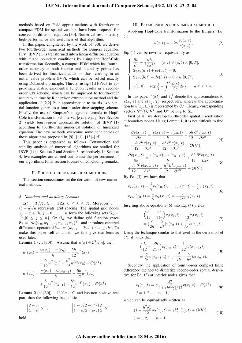
Fig. 1. Example 2 with different parameter γ (solved by Algorithm 3 with∆t = h = 0.0125): Time evolution graphs of numerical solution at t = 1.



______________________________________________________________________________________

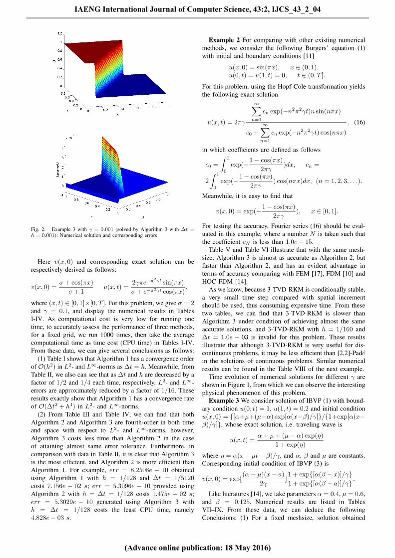
Fig. 2. Example 3 with γ = 0.001 (solved by Algorithm 3 with ∆t =h = 0.001): Numerical solution and corresponding errors

Here v(x, 0) and corresponding exact solution can berespectively derived as follows:

v(x, 0) =σ + cos(πx)

σ + 1u(x, t) =

2γπe−π2γt sin(πx)σ + e−π2γt cos(πx)

.

where (x, t) ∈ [0, 1]×[0, T ]. For this problem, we give σ = 2and γ = 0.1, and display the numerical results in TablesI-IV. As computational cost is very low for running onetime, to accurately assess the performance of three methods,for a fixed grid, we run 1000 times, then take the averagecomputational time as time cost (CPU time) in Tables I-IV.From these data, we can give several conclusions as follows:

(1) Table I shows that Algorithm 1 has a convergence orderof O(h2) in L2- and L∞-norms as ∆t = h. Meanwhile, fromTable II, we also can see that as ∆t and h are decreased by afactor of 1/2 and 1/4 each time, respectively, L2- and L∞-errors are approximately reduced by a factor of 1/16. Theseresults exactly show that Algorithm 1 has a convergence rateof O(∆t2 + h4) in L2- and L∞-norms.

(2) From Table III and Table IV, we can find that bothAlgorithm 2 and Algorithm 3 are fourth-order in both timeand space with respect to L2- and L∞-norms, however,Algorithm 3 costs less time than Algorithm 2 in the caseof attaining almost same error tolerance. Furthermore, incomparison with data in Table II, it is clear that Algorithm 3is the most efficient, and Algorithm 2 is more efficient thanAlgorithm 1. For example, err = 8.2508e − 10 obtainedusing Algorithm 1 with h = 1/128 and ∆t = 1/5120costs 7.156e − 02 s; err = 5.3096e − 10 provided usingAlgorithm 2 with h = ∆t = 1/128 costs 1.475e − 02 s;err = 5.3029e − 10 generated using Algorithm 3 withh = ∆t = 1/128 costs the least CPU time, namely4.828e− 03 s.

Example 2 For comparing with other existing numericalmethods, we consider the following Burgers’ equation (1)with initial and boundary conditions [11]

u(x, 0) = sin(πx), x ∈ (0, 1),u(0, t) = u(1, t) = 0, t ∈ (0, T ].

For this problem, using the Hopf-Cole transformation yieldsthe following exact solution

u(x, t) = 2πγ

∞∑n=1

cn exp(−n2π2γt)n sin(nπx)

c0 +∞∑

n=1

cn exp(−n2π2γt) cos(nπx)

, (16)

in which coefficients are defined as follows

c0 =∫ 1

0

exp(−1− cos(πx)2πγ

)dx, cn =

2∫ 1

0

exp(−1− cos(πx)2πγ

) cos(nπx)dx, (n = 1, 2, 3, . . .).

Meanwhile, it is easy to find that

v(x, 0) = exp(−1− cos(πx)2πγ

), x ∈ [0, 1].

For testing the accuracy, Fourier series (16) should be eval-uated in this example, where a number N is taken such thatthe coefficient cN is less than 1.0e− 15.

Table V and Table VI illustrate that with the same mesh-size, Algorithm 3 is almost as accurate as Algorithm 2, butfaster than Algorithm 2, and has an evident advantage interms of accuracy comparing with FEM [17], FDM [10] andHOC FDM [14].

As we know, because 3-TVD-RKM is conditionally stable,a very small time step compared with spatial incrementshould be used, thus consuming expensive time. From thesetwo tables, we can find that 3-TVD-RKM is slower thanAlgorithm 3 under condition of achieving almost the sameaccurate solutions, and 3-TVD-RKM with h = 1/160 and∆t = 1.0e − 03 is invalid for this problem. These resultsillustrate that although 3-TVD-RKM is very useful for dis-continuous problems, it may be less efficient than [2,2]-Padein the solutions of continuous problems. Similar numericalresults can be found in the Table VIII of the next example.

Time evolution of numerical solutions for different γ areshown in Figure 1, from which we can observe the interestingphysical phenomenon of this problem.

Example 3 We consider solution of IBVP (1) with bound-ary condition u(0, t) = 1, u(1, t) = 0.2 and initial conditionu(x, 0) = [α+µ+(µ−α) exp[α(x−β)/γ]/1+exp[α(x−β)/γ], whose exact solution, i.e. traveling wave is

u(x, t) =α + µ + (µ− α) exp(η)

1 + exp(η)

where η = α(x− µt− β)/γ, and α, β and µ are constants.Corresponding initial condition of IBVP (3) is

v(x, 0) = exp[(α− µ)(x− a)

2γ]1 + exp[α(β − x)]/γ1 + exp[α(β − a)]/γ .

Like literatures [14], we take parameters α = 0.4, µ = 0.6,and β = 0.125. Numerical results are listed in TablesVII–IX. From these data, we can deduce the followingConclusions: (1) For a fixed meshsize, solution obtained



______________________________________________________________________________________

TABLE ICOMPUTATIONAL RESULTS AT t = 1 FOR EXAMPLE 1, OBTAINED USING ALGORITHM 1 WITH ∆t = h.

h 1/4 1/8 1/16 1/32 1/64 1/128err 1.2734e− 03 1.7144e− 04 3.9949e− 05 9.8571e− 06 2.4570e− 06 6.1391e− 07rate − 2.8929 2.1015 2.0189 2.0043 2.0008err2 6.6575e− 04 1.1596e− 04 2.7471e− 05 6.7935e− 06 1.6940e− 06 4.2323e− 07rate2 − 2.5214 2.0776 2.0157 2.0037 2.0009CPU 6.312e− 05 7.900e− 05 1.260e− 04 2.810e− 04 9.070e− 04 4.907e− 03

TABLE IINUMERICAL RESULTS AT t = 1 FOR EXAMPLE 1, OBTAINED USING ALGORITHM 1.

h ∆t errerr(h,∆t)

err(0.5h,0.25∆t)err2

err2(h,∆t)err2(0.5h,0.25∆t)

CPU14

15

1.0774e− 03 − 5.4417e− 04 − 6.450e− 0518

120

5.5860e− 05 19.2874 2.9620e− 05 18.3721 9.400e− 05116

180

3.3830e− 06 16.5120 1.7829e− 06 16.6129 2.340e− 04132

1320

2.1206e− 07 15.9532 1.1044e− 07 16.1443 9.530e− 04164

11280

1.3212e− 08 16.0501 6.8870e− 09 16.0356 6.718e− 031

1281

51208.2508e− 10 16.0134 4.3022e− 10 16.0082 7.156e− 02

TABLE IIICOMPUTATIONAL RESULTS AT t = 1 FOR EXAMPLE 1 USING ALGORITHM 2 WITH ∆t = h.


TABLE IVCOMPUTATIONAL RESULTS AT t = 1 FOR EXAMPLE 1, USING ALGORITHM 3 WITH ∆t = h.


using Algorithm 1 is more accurate than the one providedusing HOC FDM [14], and needs almost the same CPU timeas HOC FDM [14]. This meets our anticipation because HOCFDM [14] has only second-order accuracy at boundary. (2)Using the same meshsize and relatively small γ, Algorithm3 has approximately as high accuracy as Algorithm 2, andis much more accurate than Algorithm 1 and HOC FDM[14]. Meanwhile, computational time of Algorithm 3 is muchlower than the one of Algorithm 2, and is roughly as muchas Algorithm 1 and HOC FDM [14]. (3) For very small γ,with the same meshsize, solution computed using Algorithm3 is more accurate than the one provided than Algorithm 2.In a word, Algorithm 3 is the most efficient in the aspectsof accuracy and computational cost.

Finally, the use of Algorithm 3 with ∆t = h = 0.001to this problem with γ = 0.001 is carried out. Evolutiongraph of numerical solution and the propagation of errors areplotted in the left and right columns of Figure 2, respectively,from which we can observe that the errors become largewhen the values of the solution vary violently. This showsthat Algorithm 3 has a good capacity of simulation for awide range of γ.

Example 4 In what follows, the IBVP (1) which has ashock-wave solution [14]

u(x, t) =λ

21 + tanh[

λ

8γ(−2x + λt)]

is solved using our methods and HOC FDM [14]. Obviously,corresponding initial condition of IBVP (3) is

v(x, 0) = exp[α(x− a)]cosh(αx)cosh(αa)

,

in which α = (−λ)/(4γ). In computation process, we chooseλ = 1.6 and boundary conditions u(−5, t) = 1.6 andu(10, t) = 0.

Numerical results listed in Table X and Table XI furthershow the evident superiority of Algorithm 3 over Algorithm2, Algorithm 1, and HOC FDM [14] in terms of accuracyand computational cost.

Figure 3 shows the graphs of numerical solutions toexample 4 with γ = 0.1 at t = 0.25, 1.5, 2.75 and thepropagation of the corresponding errors on mesh points.From this figure, we can see that the error becomes muchlarge in the vicinity of the place, where the gradient of thesolution varies very quickly.

Example 5 Finally, we consider numerical simulation ofBurgers’ equation with the initial and boundary conditions

u(x, 0) =

1, 0 ≤ x < 5,6− x, 5 ≤ x < 6,0, 6 ≤ x < 12.

and u(0, t) = 1, u(12, t) = 0. By some simple computations,



______________________________________________________________________________________

TABLE VCOMPARISONS OF L∞-ERRORS AND CPU AT t = 0.2 FOR EXAMPLE 2 WITH γ = 0.05, (∆t = h WITH EXCEPTION OF ∆t = 1.0e− 03 FOR

3-TVD-RKM).

Methods h = 1/10 (CPU) h = 1/40 (CPU) h = 1/160 (CPU)Algorithm 2 1.6837e− 03 (3.750e− 02) 6.0494e− 06 (0.589) 2.5095e− 08 (0.813)Algorithm 3 1.7097e− 03 (7.750e− 05) 6.0084e− 06 (2.350e− 04) 2.3522e− 08 (5.742e− 03)FEM [17] 3.5903e− 02) (1.870e− 05) 2.3661e− 03 (4.530e− 05) 1.4858e− 04 (6.516e− 04)FDM [10] 1.7956e− 02 (2.030e− 05) 1.1415e− 03 (4.680e− 05) 7.1605e− 05 (6.531e− 04)

HOC FDM [14] 5.8288e− 03 (1.500e− 04) 5.2591e− 04 (3.100e− 04) 3.3486e− 05 (6.400e− 03)3-TVD-RKM 1.920e− 03 (0.452) 7.0122e− 06 (0.608) NaN

TABLE VICOMPARISONS OF L2-ERRORS AND CPU AT DIFFERENT TIME LEVELS FOR EXAMPLE 2 WITH γ = 0.05, (∆t = h = 0.01 WITH EXCEPTION OF

∆t = 5.0e− 04, h = 0.01 FOR 3-TVD-RKM).

Methods t = 0.2 (CPU) t = 0.6 (CPU) t = 1.0 (CPU)Algorithm 2 8.8773e− 08 (0.515) 2.2125e− 07 (1.217) 9.8134e− 08 (1.716)Algorithm 3 8.5563e− 08 (0.171) 2.2233e− 07 (0.515) 9.7987e− 08 (0.717)FEM [17] 7.5569e− 04 (0.005) 3.5996e− 04 (0.006) 1.2426e− 04 (0.008)FDM [10] 5.7455e− 04 (0.005) 4.8370e− 05 (0.006) 3.1252e− 05 (0.008)

HOC FDM [14] 4.1443e− 05 (0.014) 1.3622e− 05 (0.015) 7.2409e− 06 (0.016)3-TVD-RKM 1.807e− 07 (0.562) 9.106e− 007 (0.624) 3.5517e− 07 (0.780)

TABLE VIICOMPARISON BETWEEN EXACT AND NUMERICAL SOLUTIONS OF EXAMPLE 3 WITH γ = 0.005 AT t = 1, (∆t = h = 0.002).

x Algorithm 1 Algorithm 2 Algorithm 3 HOC FDM [14] exact solution0.2 1.00000884705024 1.00000884705023 1.00000884705024 0.99345055174620 1.000000000000000.4 1.00000884704643 1.00000884704627 1.00000884704628 0.99345055174583 0.999999999995910.6 0.99997401773015 0.99997254089226 0.99997253343592 0.99340571924913 0.999963681705040.8 0.20206202643915 0.20197749501259 0.20197794728201 0.20178887544250 0.20197809852531err 8.3402e− 03 2.2455e− 05 1.1218e− 05 3.1874e− 02err2 1.5245e− 03 8.8047e− 06 7.4719e− 06 8.1970e− 03

TABLE VIIICOMPARISON OF NUMERICAL RESULTS AT DIFFERENT TIME LEVELS FOR EXAMPLE 3 WITH γ = 0.003, (h = 0.0025).

t = 0.2 t = 0.4 t = 0.6 t = 0.8 t = 1.0Algorithm 1 err 1.1734e− 02 2.3730e− 02 3.5815e− 02 4.7847e− 02 5.9792e− 02

∆t = h CPU 0.094 0.109 0.110 0.121 0.125Algorithm 2 err 4.1822e− 04 6.3672e− 04 7.9259e− 04 1.0129e− 03 1.3136e− 03

∆t = h CPU 0.293 0.325 0.356 0.387 0.434Algorithm 3 err 4.0566e− 04 5.4574e− 04 5.5112e− 04 5.3979e− 04 5.2724e− 04

∆t = h CPU 0.091 0.105 0.112 0.122 0.123HOC FDM [14] err 3.4087e− 02 3.4087e− 02 8.4274e− 02 1.4105e− 01 1.9799e− 01

∆t = h CPU 0.093 0.094 0.109 0.110 0.1213-TVD-RKM err 4.0663e− 04 5.4763e− 04 5.5396e− 04 5.4358e− 04 5.3197e− 04

∆t = 5.0e− 04 CPU 3.781 7.389 10.767 14.181 17.740

we have that

v(x, 0) =

exp(−x

2γ), 0 ≤ x < 5,

exp(x2

4γ− 3x

γ+

254γ

), 5 ≤ x < 6,

exp(−114γ

), 6 ≤ x < 12.

for this case.Algorithm 3 is applied to solve this problem. Profiles of

numerical solution at t = 1, 2, 3, 4 are displayed in Figure 4,which is similar to the patterns of Figure 1 and Figure 2 in[21]. This exactly confirms that numerical solution obtainedusing Algorithm 3 can exhibit correct physical behavior.

VI. CONCLUSIONS

In this article, three numerical solvers (i.e. Algorithm 1,Algorithm 2, Algorithm 3) for solving Burgers’ equationin one dimension based on Hopf-Cole transformation havebeen developed. Numerical results show the superiority ofAlgorithm 3 over Algorithm 1 and Algorithm 2 in term

of computational efficiency, though Algorithm 2 has thesame accuracy as Algorithm 3. Also, numerical results revealthat Algorithm 3 outperforms numerical solvers devised in[10], [14], [17]. However, as exact solution is not smoothenough or discontinuous, the presented methods can notattain the claimed accuracy, even invalid. As we know,the initial or/and boundary condition has jumps, the exactsolution to Burgers’ equation is discontinuous, i.e. shockwave. The proposed methods, which do not satisfy totalvariation diminishing property [31], thus yielding seriouslyspurious oscillations near discontinuities, are not suitable fornumerical simulations of discontinuous problems. This is aregretful deficiency. In the future work, it is possible to paymuch more attention to the study of exponential integrators[32], [33] with TVD property.

In addition, over the past several decades, stabilizedexplicit Runge-Kutta methods (SERKMs) [34], [35] haveattracted much more attention. They possess large stabilitydomains and have been proven to be very useful in thesolutions of IBVPs. Also, it is very interesting and challeng-ing to solve multi-dimensional IBVPs by the combinations



______________________________________________________________________________________

TABLE IXCOMPARISON OF NUMERICAL RESULTS AT t = 1 FOR EXAMPLE 3 WITH DIFFERENT γ , (∆t = h = 0.002).

γ = 0.01 γ = 0.008 γ = 0.006 γ = 0.004 γ = 0.002Algorithm 1 err 3.2528e− 03 2.6712e− 03 4.8987e− 03 1.6257e− 02 1.2838e− 01

err2 8.4138e− 04 6.1754e− 04 9.8071e− 04 2.6583e− 03 1.4968e− 02Algorithm 2 err 2.2112e− 03 6.3690e− 04 7.5088e− 05 1.0588e− 04 5.3862e− 03

err2 5.7237e− 04 1.4739e− 04 1.5553e− 05 2.4448e− 05 6.6394e− 04Algorithm 3 err 2.2112e− 03 6.3699e− 04 7.4626e− 05 4.6404e− 05 1.7570e− 03

err2 5.7238e− 04 1.4743e− 04 1.5562e− 05 1.9288e− 05 3.4468e− 04HOC FDM [14] err 2.6558e− 03 8.0053e− 03 1.9081e− 02 5.9661e− 02 3.7600e− 01

err2 1.5423e− 03 2.9058e− 03 5.5360e− 03 1.3245e− 02 5.6780e− 02

TABLE XCOMPARISON BETWEEN EXACT AND NUMERICAL SOLUTIONS OF EXAMPLE 4 WITH γ = 0.25 AT t = 1.5, (∆t = h = 0.025).

x Algorithm 1 Algorithm 2 Algorithm 3 HOC FDM [14] exact solution0 1.56637702742831 1.56633382966077 1.56633382656578 1.56637363394596 1.56633384476725

1.25 0.73665723258733 0.73613585176191 0.73613590308168 0.73665722340424 0.736136184711092.5 0.02462008147105 0.02458829874397 0.02458830650549 0.02462008147077 0.02458832890444err 5.2435e− 04 4.6538e− 07 4.6537e− 07 2.1576e− 03err2 1.2359e− 04 1.6947e− 07 1.6482e− 07 6.4710e− 04CPU 0.378 1.128 0.391 0.375

TABLE XICOMPARISON BETWEEN EXACT AND NUMERICAL SOLUTIONS OF EXAMPLE 4 WITH γ = 0.05 AT t = 1.5, (∆t = h = 0.025).

x Algorithm 1 Algorithm 2 Algorithm 3 HOC FDM [14] exact solution0 1.59999999377673 1.59999999266475 1.59999999264451 1.59999999322371 1.59999999266051

1.25 0.55398528835588 0.49472699352290 0.49527918783689 0.55398528835588 0.496040830195801.5 0.01536819730726 0.01297644607361 0.01302853320031 0.01536819730727 0.01306011384506err 6.3569e− 02 1.3138e− 03 9.2627e− 04 6.5569e− 02err2 6.9271e− 03 1.5405e− 04 1.3003e− 04 1.6828e− 02CPU 0.390 1.185 0.391 0.375

−5 0 5 100

0.2

0.4

0.6

0.8

1

1.2

1.4

1.6

1.8

x

U

t=2.75

t=0.25

t=1.5

−5 0 5 10−10

−8

−6

−4

−2

0

2

4x 10

−4

x

Err

or

t=0.25 t=1.25 t=2.75

Fig. 3. Example4 with γ = 0.1 (solved by Algorithm 3 with ∆t = h =0.05): Numerical solution and corresponding errors.

0 2 4 6 8 10 120

0.1

0.2

0.3

0.4

0.5

0.6

0.7

0.8

0.9

1

x

U

t=1

t=2

t=3

t=4

γ=1, h=∆ t=0.05

00.2

0.40.6

0.81

0

0.2

0.4

0.6

0.8

10

0.2

0.4

0.6

0.8

1

xt

U

γ=0.1

Fig. 4. Example 5 (solved by Algorithm 3 ): Numerical solutions atdifferent time levels.



______________________________________________________________________________________

of SERKMs with HOC FDMs. It is possible that sometechniques developed in this paper are useful for the researchof SERKMs combined with HOC FDMs in future.

Finally, the extensions of the proposed methods to somehigh-dimensional Burgers equations [36], [37] are impossibleif they are not transformed into heat equation with mixedboundary by Hopf-Cole transformation. Of course, similartechniques may be generalized to the following system oftwo-dimensional Burgers equations:

ut + uux + vuy = ∆uvt + uvx + vvy = ∆v

with potential symmetry condition uy = vx because it canbe transformed into heat equation by Hopf-cole transfor-mation. However, for higher complicated matrix, it is alsochallenging to investigate the good approximation of matrixexponentials.

REFERENCES

[1] H. Bateman, “Some recent researchs on the motion of fluids,” MonthlyWeather Review, vol. 43, pp. 163–170, 1915.

[2] J.M. Burgers, “Mathematical examples illustrating relations occurringin the theory of turbulent fluid motion,” Trans. Roy. Neth. Acad. Sci.Amsterdam, vol. 17 pp. 1–53, 1939.

[3] J.M. Burgers, “A mathematical model illustrating the theory of turbu-lence,” Advances in Applied Mechanics, vol. 1 pp. 171–199, 1948.

[4] E. Benton, and G.W. Platzman, “A table of solutions of the one-dimensional Burgersequations,” Quarterly of Applied Mathematics, vol.30 pp. 195–212, 1972.

[5] J.D. Cole, “On a quasi-linear parabolic equations occuring in aerody-namics,” Quarterly of Applied Mathematics, vol. 9 pp. 225–236, 1951.

[6] E. Hopf, “The partial differential equqation ut + uux = µuxx,”Communications on Pure and Applied Mathematics, vol. 3 pp. 201–230, 1950.

[7] N. Taghizadeh, M. Akbari, and A. Ghelichzadeh, “Exact solution ofBurgers squations by Homotopy perturbation method and reduceddifferential transformation method,” Australian Journal of Basic andApplied Sciences, vol. 5 pp. 580–589, 2011.

[8] Y. Jin, M. Jia, and S. Lou, “Baklund transformations and interactionsolutions of the Burgers equation,” Chinese Physics letter, vol. 30020203, 2013.

[9] I.A. Hassanien, A.A. Salama, and H.A. Hosham, “Fourth-order finitedifference method for solving Burgers’ equation,” Applied Mathematicsand Computation, vol. 170 pp. 781–800, 2005.

[10] Mohan. K. Kadalbajoo, and A. Awasthi, “A numerical method basedon Crank-Nicolson scheme for Burgers equation,” Applied Mathematicsand Computation, vol. 182 pp. 1430–1442, 2006.

[11] W. Liao, and J. Zhu, “An implicit fourth-order compact finite differ-ence scheme for one-dimensional Burgers’ equation,” Applied Mathe-matics and Computation, vol. 206 pp. 755–764, 2008.

[12] D.K. Salkuyeh, and F.S. Sharafeh, “On the numerical solution of theBurgers’s equation,” International Journal of Computer Mathematics,vol. 86 pp. 1334–1344, 2009.

[13] M. Sari, and G. Gurarslan, “A sixth-order compact finite differencescheme to the numerical solutions of Burgers equation,” AppliedMathematics and Computation, vol. 208 pp. 475–483, 2009.

[14] S. Xie, G. Li, and S. Heo, “A compact finite difference methodfor solving Burgers’ equation,” International Journal for NumericalMethods in Fluids, vol. 62 pp. 747–764, 2010.

[15] M. Yousuf, “On the class of high order time stepping schemesbaded on Pade approxiamtions for the numerical solution of Burgers’equation,” Applied Mathematics and Computation, vol. 205 pp. 442–453, 2008.

[16] S. Kutluay, A. Esen, and I. Dagb, “Numerical solutions of the Burgersequation by the least-squares quadratic B-spline finite element method,”Journal of Computational and Applied Mathematics, vol. 167 pp. 21–33, 2004.

[17] T. Ozis, E.N. Aksan, and A. Ozdes, “A finite element approach forsolution of Burgers’ equation,” Applied Mathematics and Computation,vol. 139 pp. 417–428, 2003.

[18] L. Shao, X. Feng, and Y. He, “The local discontinuous Galerkin finiteelement method for Burgers equation,” Mathematical and ComputerModelling, vol. 54 pp. 2943–2954, 2011.

[19] R. Zhang, X. Yu, and G. Zhao, “Local discontinuous Galerkin methodfor solving Burgers and coupled Burgers equations,” Chinese PhysicsLetter, vol. 20 110205, 2011.

[20] C. Basdevant, M. Devilie, and P. Haldenwang, et. al., “Spectral andfinite difference solutions of the Burger equation,” Computer & Fluids,vol. 14 pp. 23–41, 1986.

[21] R.C. Mittal, and P. Singhal, “Numerical solution of Burger’s equation,”Communications in Numerical Methods in Engineering, vol. 9 pp. 397–406, 1993.

[22] S. Chen, X. Wu, Y. Wang, and W. Kong, “The Laplace transformmethod for Burgers’ equation,” International Journal for NumericalMethods in Fluids, vol. 63, 1060–1076, 2010.

[23] A. Hashemian, and H.M. Shodja, “A meshless approach for solution ofBurgers equation,” Journal of Computational and Applied Mathematics,vol. 220 pp. 226–239, 2008.

[24] A. Korkmaz, and I , “Dag, Polynomial based differential quadraturemethod for numerical solution of nonlinear Burgers equation,” Journalof the Franklin Institute, vol. 348 pp. 2863–2875, 2011.

[25] R. Mokhtari, A.S. Toodar, and N.G. Chegini, “Application of the gen-eralized differential quadrature method in solving Burgers’equations,Communications in Theoretical Physics vol. 56 pp. 1009–1015, 2011.

[26] R.K. Lele, “Compact finite difference schemes with spectral-likeresolution,” Journal of Computational Physics, vol. 103 pp. 16–42,1992.

[27] D. Deng, and T. Pan, ”A Fourth-order Singly Diagonally ImplicitRunge-Kutta Method for Solving One-dimensional Burgers’ Equation,”IAENG International Journal of Applied Mathematics, vol. 45, no. 4,pp. 327–333, 2015.

[28] B. Wongsaijai, K. Poochinapan, and T. Disyadej, “A compact finitedifference methodfor solving the general Rosenau-RLW Equation,”IAENG International Journal of Applied Mathematics, vol. 44, no. 4,pp. 192-199, 2014.

[29] J.C. Chen and W. Chen, “Two-dimensional nonlinear wave dynamicsin blasius boundary layer flow using combined compact differencemethods,” IAENG International Journal of Applied Mathematics, vol.41, no. 2, pp. 162-171, 2011.

[30] H. Cao, L. Liu, Y. Zhang, and S. Fu, “A fourth-order method ofthe convection-diffusion equations with Neumann boundary conditions,”Applied Mathematics and Computation, vol. 217 pp. 9133–9141, 2011.

[31] Y. Hadjimichael, C. B. Macdonald, D. I. Ketcheson, and J. H. Verner,“Strong stability preserving explicit Runge-Kutta methods of maximaleffective order,” SIAM Journal on Numerical Analysis, vol. 51 pp.2149–2165, 2013.

[32] M. Hochbruck, Ch. Lubich, and H. Selhofer. “Exponential integratorsfor large systems of differential equations,” SIAM Journal on ScientificComputing, vol. 19 pp. 1552–1574, 1998.

[33] A.Q.M. Khaliq, J. Martn-Vaquero, B.A.Wade, and M. Yousuf.“Smoothing schemes for reaction-diffusion systems with nonsmoothdata,” Journal of Computational and Applied Mathematics, vol. 223pp. 374–386, 2009.

[34] B. Kleefeld, and J. Martın-Vaquero, “Serk2v2: A new second-orderstabilized explicit Runge-Kutta method for stiff problems,” NumericalMethods for Partial Differential Equations, vol. 29 pp. 170–185, 2013.

[35] J. Martın-Vaquero, A.Q.M. Khaliq, and B. Kleefeld, “Stabilized ex-plicit Runge-Kutta methods for multi-asset American options,” Com-puters & Mathematics with Applications, vol. 67 pp. 1293–1308, 2014.

[36] C.h. Dai, and F.B. Yu, “Special solitonic localized structures for the(3+1)- dimensional burgers equation in water waves,” Wave Motion,vol. 51 pp. 52–59, 2014.

[37] A. Wazwaz, Multiple kink solutions for M-component Burgers equa-tions in (1+1)-dimensions and (2+1)-dimensions, Applied Mathematicsand Computation, 217 pp. 3564–3570, 2010.



______________________________________________________________________________________

high-order exponential time differencing methods … exponential time differencing methods for...

Documents