high performance computing - tu wien
TRANSCRIPT

©Jesper Larsson TräffWS20
1
High Performance ComputingIntroduction, overview
High Performance ComputingIntroduction, overview
Jesper Larsson Träfftraff@par. …
Institute of Computer Engineering, Parallel Computing, 191-4Favoritenstrasse 16, 3. Stock

©Jesper Larsson TräffWS20
2
High Performance Computing: A (biased) overview
Concerns: Either
1. Achieving highest possible performance as needed by some application(s)
2. Getting highest possible performance out of given (highly parallel) system
• Ad 1: Anything goes, including designing and building new systems, raw application performance matters
• Ad 2: Understanding and exploiting details at all levels of given system

©Jesper Larsson TräffWS20
3
• Understanding modern processors: Processor architecture, memory system, single-core performance, multi-core parallelism
• Understanding parallel computers: Communication networks
• Programming parallel systems efficiently and effectively: Algorithms, interfaces, tools, tricks
All issues at all levels are relevant
…but not always to the same extent and at the same time
Ad. 2
Our themes for this lecture

©Jesper Larsson TräffWS20
4
Traditional “Scientific Computing”/HPC applications
• Weather• Long-term weather forecast• Climate (simulations: coupled models, multi-scale, multi-
physics)• Earth Science
• Nuclear physics• Computational chemistry, Computational astronomy,
Computational fluid dynamics, …
• Protein folding, Molecular Dynamics (MD)
• Cryptography (code-breaking, NSA)• Weapons (design, nuclear stock pile), defense (“National
Security”), spying (NSA), …
Qualified estimates say these problems require TeraFLOPS, PetaFLOPS, ExaFLOPS, …

©Jesper Larsson TräffWS20
5
Other, newer High-Performance Computing applications
• Machine Learning (ML), Deep Neural Networks (DNN) or other
• Data analytics (Google, Amazon, FB, …), “big data”
• Irregular data (graphs), irregular access patterns (graph algorithms)
Applications have different characteristics (operations, loops, tasks, access patterns, locality) and requirements (computation, memory, communication).Different HPC architecture trade-offs for different applications

©Jesper Larsson TräffWS20
6
Ad. 1: Special purpose HPC systems for Molecular Dynamics
Special purpose computers have a history in HPC (computer science in general)
“Colossus” replica, Tony Sale 2006: Enigma code breaking
Thomas Haigh: Colossal genius: Tutte, Flowers, and a bad imitation of Turing. Commun. ACM 60(1): 29-35 (2017)Henry Shipley: Turing: Colossus computer revisited. Nat. 483(7389): 275 (2012)
©Jesper Larsson TräffWS20
7
N-body computations of forces between molecules to determine movements: Special type of computation with specialized algorithms that could potentially be executed orders of magnitude more efficiently (time, energy) on special-purpose hardware
Example: N-body problem
M. Snir: “A Note on N-Body Computations with Cutoffs”. Theory Comp. Syst. 37(2): 295-318,2004
©Jesper Larsson TräffWS20
8
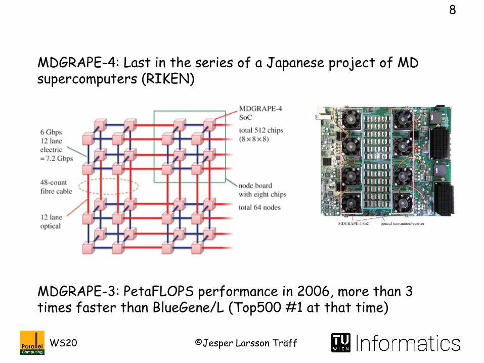
MDGRAPE-3: PetaFLOPS performance in 2006, more than 3 times faster than BlueGene/L (Top500 #1 at that time)
MDGRAPE-4: Last in the series of a Japanese project of MD supercomputers (RIKEN)
©Jesper Larsson TräffWS20
9
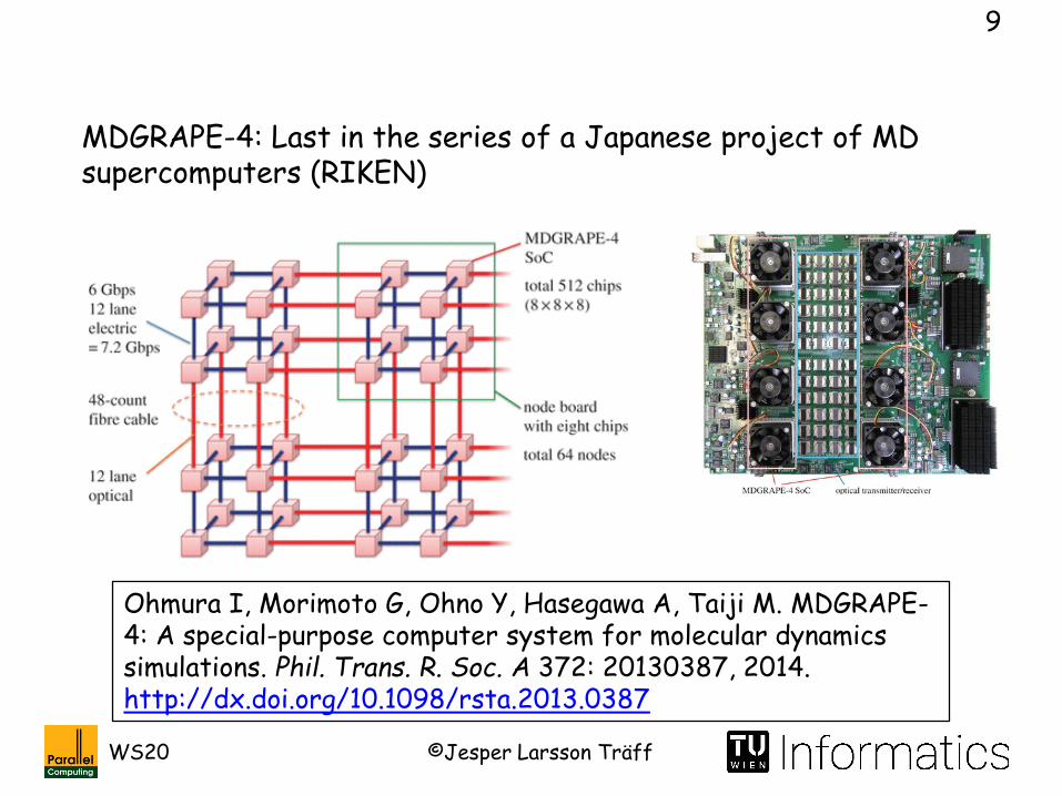
MDGRAPE-4: Last in the series of a Japanese project of MD supercomputers (RIKEN)
Ohmura I, Morimoto G, Ohno Y, Hasegawa A, Taiji M. MDGRAPE-4: A special-purpose computer system for molecular dynamics simulations. Phil. Trans. R. Soc. A 372: 20130387, 2014. http://dx.doi.org/10.1098/rsta.2013.0387

©Jesper Larsson TräffWS20
10
Anton (van Leeuwenhoek): Another special purpose MD system
512-node (8x8x8 torus) Anton machine
D. E. Shaw Research (DESRES)
Special purpose Anton chip (ASIC)

©Jesper Larsson TräffWS20
11
From “Encyclopedia on Parallel Computing”, Springer 2011:
“Prior to Anton’s completion, few reported all-atom protein simulations had reached 2μs, the longest being a 10-μs simulation that took over 3 months on the NCSA Abe supercomputer […]. On June 1, 2009, Anton completed the first millisecond-long simulation – more than 100 times longer than any reported previously.”

©Jesper Larsson TräffWS20
12
J. P. Grossman, Brian Towles, Brian Greskamp, David E. Shaw: Filtering, Reductions and Synchronization in the Anton 2 Network. IPDPS 2015: 860-870Brian Towles, J. P. Grossman, Brian Greskamp, David E. Shaw: Unifying on-chip and inter-node switching within the Anton 2 network. ISCA 2014: 1-12
David E. Shaw, Martin M. Deneroff, Ron O. Dror, Jeffrey Kuskin, Richard H. Larson, John K. Salmon, Cliff Young, Brannon Batson, Kevin J. Bowers, Jack C. Chao, Michael P. Eastwood, Joseph Gagliardo, J. P. Grossman, Richard C. Ho, Doug Ierardi, IstvánKolossváry, John L. Klepeis, Timothy Layman, Christine McLeavey, Mark A. Moraes, Rolf Mueller, Edward C. Priest, Yibing Shan, Jochen Spengler, Michael Theobald, Brian Towles, Stanley C. Wang: Anton, a special-purpose machine for molecular dynamics simulation. Commun. ACM 51(7): 91-97 (2008)
Ron O. Dror, Cliff Young, David E. Shaw: Anton, A Special-Purpose Molecular Simulation Machine. Encyclopedia of Parallel Computing 2011: 60-71
©Jesper Larsson TräffWS20
13
Recent Anton 2 installation:
Pittsburg Supercomputing Center (PSC), see• https://www.psc.edu/resources/computing/anton• https://www.psc.edu/news-publications/2181-anton-2-will-
increase-speed-size-of-molecular-simulations

©Jesper Larsson TräffWS20
14
Ad. 1: Special purpose HPC for Deep Neural Network processing
Google TensorFlow processors (TPU) for DNN• TPUv1: inference (2018): claims 15-30 times faster, 30-80
times more energy efficient that CPU/GPU
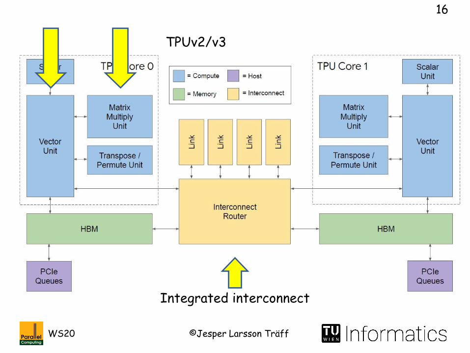
• TPUv2, v3: training (2020), 10 times performance/watt gains over Top500 supercomputers
Norman P. Jouppi, Doe Hyun Yoon, George Kurian, Sheng Li, Nishant Patil, James Laudon, Cliff Young, David A. Patterson:A domain-specific supercomputer for training deep neural networks. Commun. ACM 63(7): 67-78 (2020)
Norman P. Jouppi, Cliff Young, Nishant Patil, David A. Patterson: A domain-specific architecture for deep neural networks. Commun. ACM 61(9): 50-59 (2018)Norman P. Jouppi, Cliff Young, Nishant Patil, David A. Patterson: Motivation for and Evaluation of the First Tensor Processing Unit. IEEE Micro 38(3): 10-19 (2018)

©Jesper Larsson TräffWS20
15
TPUv1
Systolic array MM processor
©Jesper Larsson TräffWS20
16
Integrated interconnect
TPUv2/v3
©Jesper Larsson TräffWS20
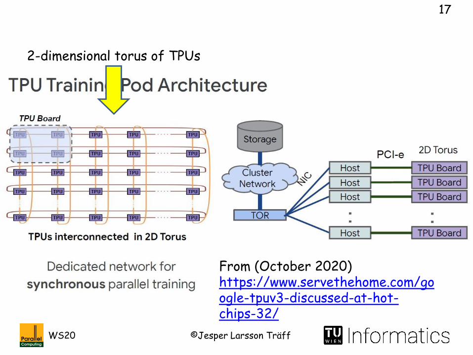
17
2-dimensional torus of TPUs
From (October 2020)https://www.servethehome.com/google-tpuv3-discussed-at-hot-chips-32/

©Jesper Larsson TräffWS20
18

©Jesper Larsson TräffWS20
19
Special purpose architectures
• Dedicated functional units for special types of operations (FMA, MV, MM, …)
• Special ISA (special compiler support), often VLIW• Special (short?) data formats• Aggressive, special memory system
Special purpose/general purpose (Turing complete): Matter of degree• Standardized ISA• Balanced memory system, balanced communication system• General data formats• …
John L. Hennessy, David A. Patterson: A new golden age for computer architecture. Commun. ACM 62(2): 48-60 (2019)
Turing Award lecture 2018

©Jesper Larsson TräffWS20
20
Ad 1.: Special purpose to general purpose
Special purpose sometimes have wider applicability
Special purpose advantages:• Higher performance (FLOPS) for special types of
computations/applications• More efficient (energy, number of transistors, …)
• Graphics processing processors (GPU) for general purpose computing (GPGPU)
• Field Programmable Gate Arrays (FPGA)
HPC systems: Special purpose processors as accelerators (GPU, FPGA, Xeon Phi, …)

©Jesper Larsson TräffWS20
21
General purpose MD software packages
• GROMACS, www.gromacs.org• NAMD, www.ks.uiuc.edu/Research/namd/
©Jesper Larsson TräffWS20
22
• Dense and sparse matrices, linear equations• PDE (“Partial Differential Equations”, multi-grid methods)• N-body problems (MD again)• …
• Many (parallel) support libraries: • BLAS -> LAPACK -> ScaLAPACK• Intel’s MKL (Math Kernel Library)
• MAGMA/PLASMA
• FLAME/Elemental/PLAPACK [R. van de Geijn]
Other typical components in scientific computing applications
• PETSc (“Portable Extensible Toolkit for Scientific computation”)

©Jesper Larsson TräffWS20
23
Ad. 2: Template High-Performance Computing architecture
Georg Hager, Gerhard Wellein: Introduction to High Performance Computing for Scientists and Engineers. Chapman and Hall / CRC computational science series, CRC Press 2011, ISBN 978-1-439-81192-4, pp. I-XXV, 1-330
• Typical elements of modern, parallel (High-Performance Computing) architectures: “A qualitative approach”
• Balance: Which architecture for which applications?
• Levels of parallelism
• Parallelism in programming model/interface

©Jesper Larsson TräffWS20
24
L1
Lk
Main memory
Communication network
L1 L1
Lk
L1
SIMD
Acc
L1
Lk
Main memory
L1 L1
Lk
L1
SIMD
Acc
• Hierarchical designs: core, processor, node, rack, island, …• Orthogonal capabilities: Accelerators, vectors • Different types parallelism at all levels
NIC NIC

©Jesper Larsson TräffWS20
25
L1
Lk
Main memory
Communication network
L1 L1
Lk
L1
SIMD
Acc
L1
Lk
Main memory
L1 L1
Lk
L1
SIMD
Acc
• Total number of cores (what counts as a core?)• Size of memories• Properties of communication network
NIC NIC

©Jesper Larsson TräffWS20
26
Main memory
Lk
L1
SIMD
Acc
Memory hierarchy
• Compute performance: How many instructions can each core perform per clock cycle (superscalar≥1)
• Special instructions&FUs: Vector, SIMD, FMA, (CISC…)• Accelerator (if integrated in core)
Parallelism in core:• Implicit, hidden (ILP)• Explicit SIMD• Explicit accelerator (GPU)How expressed, exploited?

©Jesper Larsson TräffWS20
27
Compute performance measured in FLOPS: Floating Point Operations per Second
Floating Point: In HPC almost always 64-bit IEEE Floating Point number (32 bits too little for many scientific applications, but not all!)
FLOPS
M(ega)FLOPS 106
G(iga)FLOPS 109
T(era)FLOPS 1012
P(eta)FLOPS 1015
E(xa)FLOPS 1018
Z(etta)FLOPS 1021
Y(otta)FLOPS 1024
System peak Floating Point Performance (Rpeak)
Definition (HW peak performance):Rpeak ≈ClockFrequency x #FLOP/Cycle x#CPU’s x #Cores/CPU
Optimistic, best case upper bound

©Jesper Larsson TräffWS20
28
Main memory
Lk
L1
SIMD
• Compute performance: How many instructions can core perform per clock cycle (superscalar≥1)
• Special instructions&FUs: Vector, SIMD (v≥1 operations per cycle)
Vector processor:Performance from wide SIMD unit
High performance for applications with large vectors
Memory hierarchySuperscalar: Multiple pipelines (integer, logical, FP add, FP mul, …
Requires right mix of instructions

©Jesper Larsson TräffWS20
29
Parallelism through• Pipelining: Also complex
instructions can be delivered once per cycle. Problem: dependencies, branches
• Multiple pipelines: Several different, independent instructions can be executed concurrently
Superscalar: Multiple pipelines (integer, logical, FP add, FP mul, …

©Jesper Larsson TräffWS20
30
Main memory
Lk
L1
SIMD
Acc
• Compute performance: How many instructions can core perform per clock cycle (superscalar≥1)
• Special instructions&FUs: Vector, SIMD• Accelerator: In core or external (e.g., GPU)
Heavily accelerated system, one or more accelerators
How tightly integrated with memory system/core?
High performance for applications that fit with accelerator model Acc memory
Memory hierarchy

©Jesper Larsson TräffWS20
31
Main memory
Lk
L1
SIMD
Acc
• Memory hierarchy: Latency (number of cycles to access first Byte), Bandwidth (Bytes/second)
• Balance between compute performance and memory bandwidth
• Memory access times not uniform (NUMA)
Memory hierarchy

©Jesper Larsson TräffWS20
32
Definition (HW Peak Performance):
Rpeak ≈ ClockFrequency x #FLOP/Cycle x #CPU’s x #Cores/CPU
Definition:The hardware efficiency is the ratio Rmax/Rpeak, with Rmax the measured (sustained) application performance, Rpeak the nominal HW peak performance
Measured application performance (sustained performance): How many FLOPS does application achieve on system?
Note: This efficiency measure is totally different from the algorithmic efficiency E = SU/p
What if efficiency « 1?

©Jesper Larsson TräffWS20
33
Main memory
Lk
L1
SIMD
Acc
Application is:• Compute bound, if number of FLOPs per Byte read+written
larger than memory bandwidth• Memory bound, if number of FLOPs per Byte read+written
smaller than memory bandwidth
Memory hierarchy

©Jesper Larsson TräffWS20
34
Given application (kernel) A:
Arithmetical (Operational) intensity OI:Count (average) number of (Floating Point) OPerations per Byte read/written
Required BW, RB: HW Performance in (FL)OPS divided by OI
Memory bound: RB > MBCompute bound: RB < MB
Property of application
a = x*x+2*x*x*x+3*x*x*x*x+4*x*x*x*x*x;
Performance and memory bandwidth (MB) properties of processor and memory system
Example: Calculate RB on 2GHz, not superscalar processor, 64-bit Float
OI = 16/(2*8) = 1 FLOP/Byte, RB = 2GByte/s Can memory system deliver?

©Jesper Larsson TräffWS20
35
L1
Lk
Main memory
L1 L1
Lk
L1
SIMD
Acc
Memory hierarchy
Multi-core CPU
• Cache hierarchy: 2, 3, 4, … levels: How to exploit efficiently (capacity, associativity, …)?
• Caches shared at certain levels (different in different processors, e.g., AMD, Intel, …)
• Caches coherent?• Memory typically (very) NUMA
Cache management most often transparent (done by CPU); can have hugeperformance impact.
Applications do not benefit equally well from cache system
Shared memory parallelism (OpenMP, threads, MPI, …)

©Jesper Larsson TräffWS20
36
L1
Lk
Main memory
Communication network
L1 L1
Lk
L1
SIMD
Acc
NIC
Properties of communication network:• Latency (time to initiate communication, first Byte),
Bandwidth (Bytes/second) or time per unit• Contention?
• How powerful is the network (performance, capabilities)?
• How is communication network integrated with memory and processor?
• What can communication coprocessor (NIC) do?
• Possible to overlap communication and computation?
©Jesper Larsson TräffWS20
37
L1
Lk
Main memory
Communication network
L1 L1
Lk
L1
SIMD
Acc
NIC
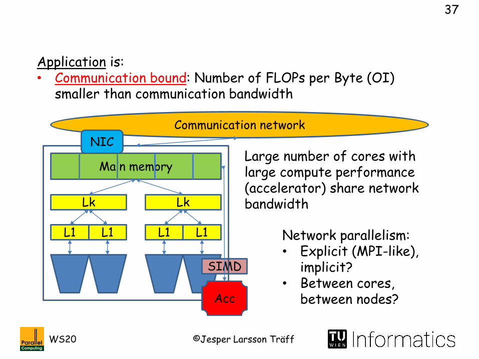
Application is:• Communication bound: Number of FLOPs per Byte (OI)
smaller than communication bandwidth
Large number of cores with large compute performance (accelerator) share network bandwidth
Network parallelism:• Explicit (MPI-like),
implicit?• Between cores,
between nodes?

©Jesper Larsson TräffWS20
38
Roofline model: How well does application exploit given HW?
1. Estimate HW peak performance, in (FL)OPS2. Estimate (main) memory bandwidth, in Bytes/s
3. Roof 1: Compute and plot Memory Performance as function of OI:
Memory Performance (in (FL)OPS) = OI (Operations/Byte)*BW (Bytes/s)
4. Roof 2: Plot HW peak performance as function of OI (constant)
Architectural HW roofs
Definition: The (OI,Roof) plot is the roofline model for the given architecture

©Jesper Larsson TräffWS20
39
1. Estimate OI (arithmetical/operational intensity)
2. Measure achieved performance of application (FLOPS)
The application/kernel/algorithm/implementation
The (OI,Performance) is one point in the roofline model: If this point is close to a roof, the application is exploiting the HW (memory system, compute capability) well
Roofline model (most often): log-log plot

©Jesper Larsson TräffWS20
40
“Theoretical” roofline analysis:Inspect kernel, algorithm, application: How many FLOPs per Byte read+written. Use specifications of hardware.
“Empirical” roofline analysis:Measure memory bandwidth, e.g., STREAM benchmark.Measure OI, e.g. using hardware performance counters (how many operations of different types, how many Bytes read+written?)
Hardware performance: Study architecture, specification
©Jesper Larsson TräffWS20
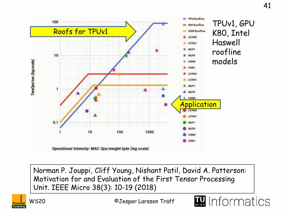
41
Norman P. Jouppi, Cliff Young, Nishant Patil, David A. Patterson: Motivation for and Evaluation of the First Tensor Processing Unit. IEEE Micro 38(3): 10-19 (2018)
TPUv1, GPU K80, Intel Haswellroofline models
Roofs for TPUv1
Application

©Jesper Larsson TräffWS20
42
Roofline analysis of application on given hardware
• If application is close to either memory or performance roofs: Exploits architecture well
• If application is close to memory roof, but far from performance roof: too low OI, rethink algorithm to do more operations per Byte read+written
• If application is far from roofs: Architecture not exploited, wrong mix of operations, no vectorization, dependencies, …

©Jesper Larsson TräffWS20
43
From https://crd.lbl.gov/departments/computer-science/par/research/roofline/introduction/

©Jesper Larsson TräffWS20
44
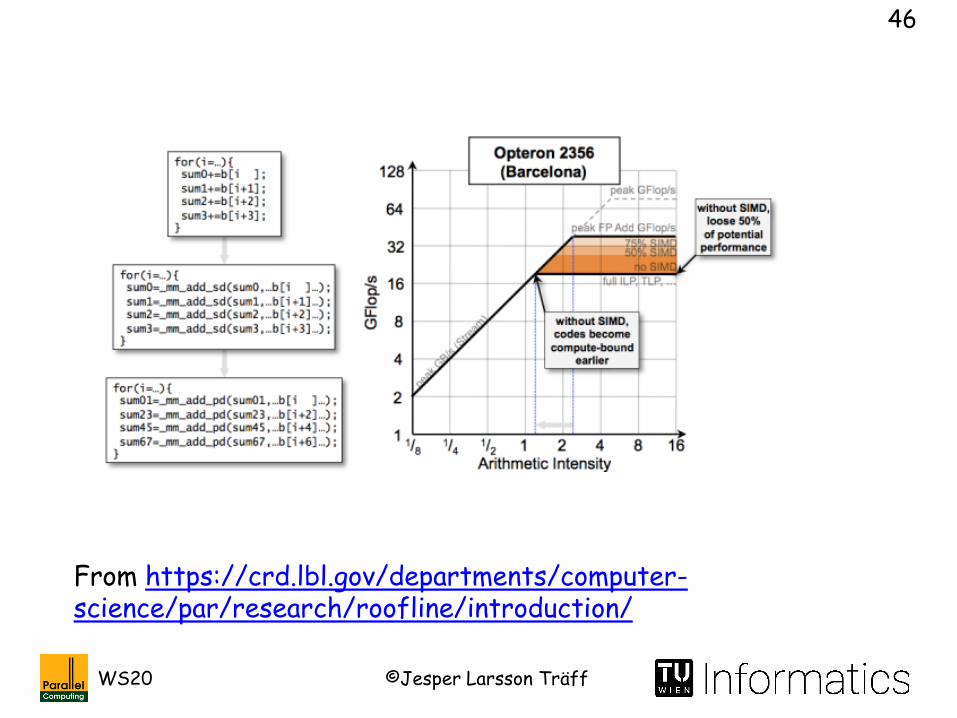
Sophisticated roofline models:
• HW roofs for different types of functional units: FMA, SIMD (avx2), …
• HW roof for different kinds of operations: FP, integer, logical
• Different types of memory (caches, L1, L2, L3, main memory)• Communication?

©Jesper Larsson TräffWS20
45
From https://crd.lbl.gov/departments/computer-science/par/research/roofline/software/ert/
©Jesper Larsson TräffWS20
46
From https://crd.lbl.gov/departments/computer-science/par/research/roofline/introduction/

©Jesper Larsson TräffWS20
47
From https://crd.lbl.gov/departments/computer-science/par/research/roofline/introduction/
©Jesper Larsson TräffWS20
48
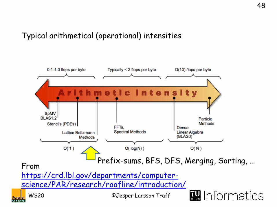
From https://crd.lbl.gov/departments/computer-science/PAR/research/roofline/introduction/
Typical arithmetical (operational) intensities
Prefix-sums, BFS, DFS, Merging, Sorting, …

©Jesper Larsson TräffWS20
49
Samuel Williams, Andrew Waterman, David A. Patterson: Roofline: an insightful visual performance model for multicore architectures. Commun. ACM 52(4): 65-76 (2009)
Nicolas Denoyelle, Brice Goglin, Aleksandar Ilic, Emmanuel Jeannot, Leonel Sousa: Modeling Non-Uniform Memory Access on Large Compute Nodes with the Cache-Aware Roofline Model. IEEE Trans. Parallel Distrib. Syst. 30(6): 1374-1389 (2019)Aleksandar Ilic, Frederico Pratas, Leonel Sousa:Beyond the Roofline: Cache-Aware Power and Energy-Efficiency Modeling for Multi-Cores. IEEE Trans. Computers 66(1): 52-58 (2017)
David Cardwell, Fengguang Song: An Extended Roofline Model with Communication-Awareness for Distributed-Memory HPC Systems. HPC Asia 2019: 26-35
Roofline model(s): References

©Jesper Larsson TräffWS20
50
Some past and present HPC architectures
Looking at Top500 list: www.top500.org
Ranks supercomputer performance by LINPACK benchmark (HPL), updated twice yearly (June, ISC Germany; November ACM/IEEE Supercomputing)

©Jesper Larsson TräffWS20
51
Serious background of Top500:Benchmarking to evaluate (super)computer performance
In HPC: Often based on one single benchmarkHigh Performance LINPACK (HPL) solves a system of linear equations under specified constraints (minimum number of operations), see www.top500.org
HPL performs well (high computational efficiency, high OI) on many architectures; allows a wide range of optimizations
HPL is less demanding on communication performance: Compute bound, OI (operational intensity) of O(n) FLOPs per Byte
HPL does not give a balanced view of “overall” system capabilities (communication)
HPL is politically important… (much money lost because of HPL…)
©Jesper Larsson TräffWS20
52
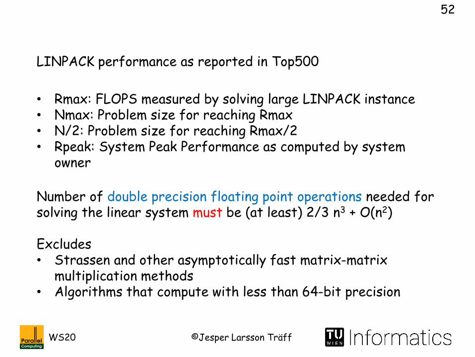
LINPACK performance as reported in Top500
• Rmax: FLOPS measured by solving large LINPACK instance• Nmax: Problem size for reaching Rmax• N/2: Problem size for reaching Rmax/2• Rpeak: System Peak Performance as computed by system
owner
Number of double precision floating point operations needed for solving the linear system must be (at least) 2/3 n3 + O(n2)
Excludes• Strassen and other asymptotically fast matrix-matrix
multiplication methods• Algorithms that compute with less than 64-bit precision

©Jesper Larsson TräffWS20
53
June 2019
#500 system
#1 system
What are the systems at the jumps?
All systems

©Jesper Larsson TräffWS20
54
June 2020
#500 system
#1 system
All systems

©Jesper Larsson TräffWS20
55
June 2020: Rank #1
System Cores Rmax(TFLOPS
Rpeak(TFLOPS)
Power(kW)
Fugaku: A64FX 48C 2.2GHz, Tofu interconnect D, Fujitsu RIKEN Center for Computational ScienceJapan
7,299,072 415,530.0 513,854.7 28,335

©Jesper Larsson TräffWS20
56
June 2019: Rank #1
System CoresRmax(TFLOPS)
Rpeak(TFLOPS)
Power (kW)
Summit: IBM Power System AC922, IBM POWER9 22C 3.07GHz, NVIDIA Volta GV100, Dual-rail MellanoxEDR Infiniband , IBM DOE/SC/Oak Ridge National LaboratoryUnited States
2,414,592 148,600.0 200,794.9 10,096

©Jesper Larsson TräffWS20
57
System CoresRmax(TFLOPS)
Rpeak(TFLOPS)
Power (kW)
Sierra: IBM Power System S922LC, IBM POWER9 22C 3.1GHz, NVIDIA Volta GV100, Dual-rail MellanoxEDR Infiniband , IBM / NVIDIA / MellanoxDOE/NNSA/LLNLUnited States
1,572,480 94,640.0 125,712.0 7,438
June 2019: Rank #2

©Jesper Larsson TräffWS20
58
November 2017: Rank #1
System CoresRmax(TFLOPS)
Rpeak(TFLOPS)
Power (kW)
SunwayTaihuLight:Sunway MPP, Sunway SW26010 260C 1.45GHz, Sunway , NRCPC National Supercomputing Center in WuxiChina
10,649,600 93,014.6 125,435.9 15,371
©Jesper Larsson TräffWS20
59
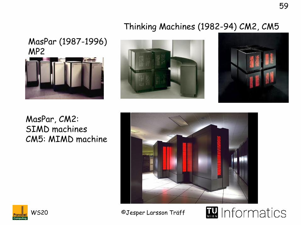
MasPar (1987-1996) MP2
Thinking Machines (1982-94) CM2, CM5
MasPar, CM2:SIMD machinesCM5: MIMD machine

©Jesper Larsson TräffWS20
60
“Top” HPC systems 1993-2000 (from www.top500.org)
©Jesper Larsson TräffWS20
61
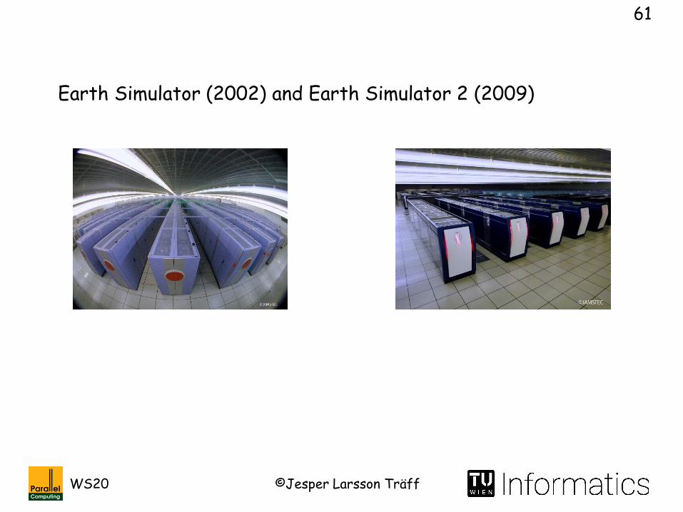
Earth Simulator (2002) and Earth Simulator 2 (2009)

©Jesper Larsson TräffWS20
62
K computer (2011) and Fugaku (2020)
©Jesper Larsson TräffWS20
63
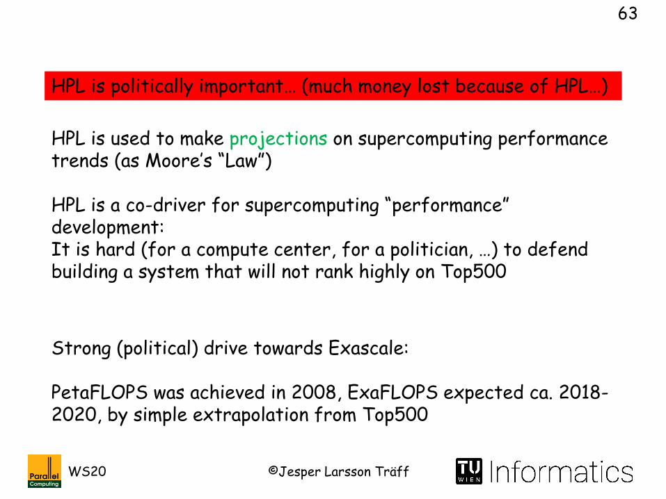
HPL is politically important… (much money lost because of HPL…)
HPL is used to make projections on supercomputing performance trends (as Moore’s “Law”)
HPL is a co-driver for supercomputing “performance” development:It is hard (for a compute center, for a politician, …) to defend building a system that will not rank highly on Top500
Strong (political) drive towards Exascale:
PetaFLOPS was achieved in 2008, ExaFLOPS expected ca. 2018-2020, by simple extrapolation from Top500

©Jesper Larsson TräffWS20
64
November 2016
According to projection, 2018/19 ExaFlop prediction will not hold
Why not? Any specific obstacles to ExaScaleperformance?

©Jesper Larsson TräffWS20
65
November 2017
According to projection, 2018/19 ExaFlop prediction will not hold
©Jesper Larsson TräffWS20
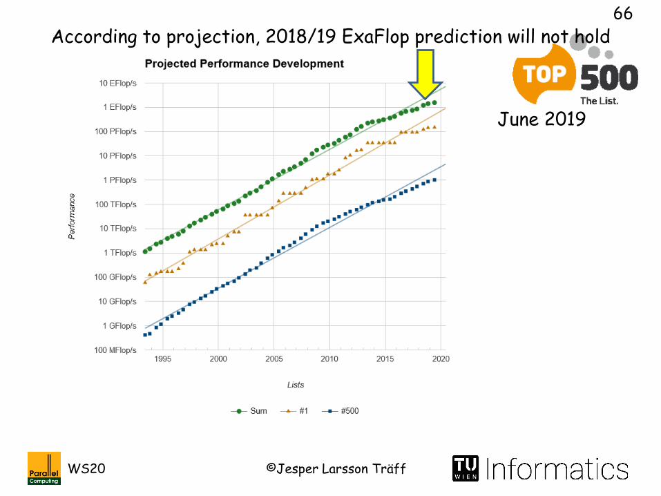
66
June 2019
According to projection, 2018/19 ExaFlop prediction will not hold

©Jesper Larsson TräffWS20
67
June 2020
©Jesper Larsson TräffWS20
68
HPCC: www.hpcchallenge.org: Benchmark suite (DGEMM, STREAM, PTRANS, Random Access, FFT, B_Eff)HPCG: http://hpcg-benchmark.orgHPGMG: https://crd.lbl.gov/departments/computer-science/PAR/research/hpgmg
Graph500 (Graph search, BFS): www.graph500.orgGreen500 (Energy consumption/efficiency): www.green500.org
Other HPC systems benchmarks
Intended to complement HPL or to highlight other aspects
STREAM: www.cs.virginia.edu/stream: Memory performance
Still active? Part of Top500

©Jesper Larsson TräffWS20
69
NAS Parallel Benchmarks (NPB): https://www.nas.nasa.gov/publications/npb.html: Benchmark suite of small kernels• IS: Integer sort• EP: Embarassingly parallel• CG: Conjugate Gradient• MG: Multigrid• FT: Discrete 3D Fast Fourier Transform• BT: Block tridiagonal solver• SP: Scalar Pentadioganal solver• LU: Lower-Upper factorization Gauss-Seidel solver
Often used in research papers. What is evaluated, under which conditions, and compared to what? Understand the benchmarks

©Jesper Larsson TräffWS20
70
Mini Application suite (https://mantevo.org):
• MiniAMR: Adaptive Mesh Refinement• MiniFE: Finite Elements• MiniGhost: 3D halo exchange (ghost cells) for finite
differencing• MiniMD: Molecular Dynamics• CloverLeaf: compressible Euler equations • TeaLeaf: Linear heat conduction equation

©Jesper Larsson TräffWS20
71
• Very early days: Single-processor supercomputers (vector)• After ‘94, all supercomputers are parallel computers
• Earlier days: Custom-made, unique – highest performance processor + highest performance network
• Later days, now: Custom convergence, weaker standard processors, but more of them, weaker networks (InfiniBand, Tori, …)
• Recent years: Accelerators (again): GPUs, FPGA, MIC, …
Using top500: Broad trends in HPC systems architecture
Much interesting computer history in top500 list; but also much is lost, and many details are not there. See what you can find
©Jesper Larsson TräffWS20
72
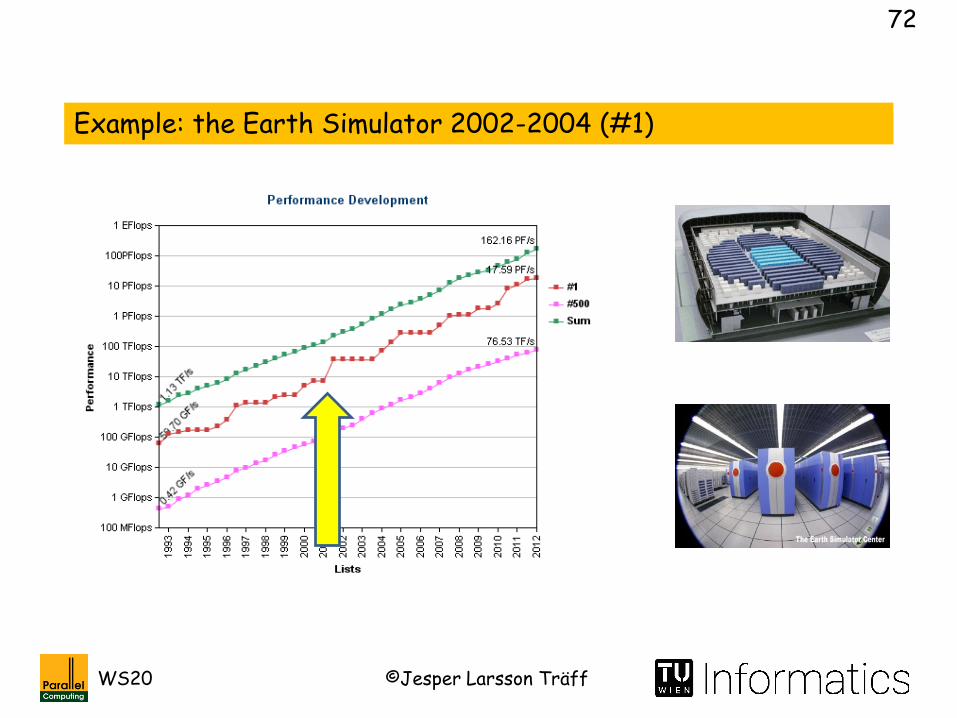
Example: the Earth Simulator 2002-2004 (#1)

©Jesper Larsson TräffWS20
73
System Vendor Cores Rmax(GFLOPS)
Rpeak(GFLOPS)
Power(KW)
Earth-Simulator
NEC 5120 35860.00 40960.00 3200.00
June 2002, Earth Simulator
• Rmax: Performance achieved on HPL• Rpeak: “Theoretical Peak Performance”, best case, all
processors fully busy
Power: Processors only (cooling, storage)?

©Jesper Larsson TräffWS20
74
Power supply
• ~40TFLOPS
• 5120 vector processors• 8 (NEC SX6) processors per node• 640 nodes, 640x640 full crossbar interconnect
BUT: Energy expensive
Earth Simulator 2 (2009) onlyvector system on Top500
• ~15MW

©Jesper Larsson TräffWS20
75
Vector processor operates on long vectors, not only scalars
Peak performance: 8GFlops (all vector pipes active)
Long vectors:256 element (double/long) vectors
Vector architecture pioneered by Cray (Cray-1 1976, late 60ties, early 70ties). Other vendors: Convex, Fujitsu, NEC, …

©Jesper Larsson TräffWS20
76
Main memory
SIMD
• One instruction• Several, deep pipelines can be kept busy by long vector
registers, no branches, no pipeline stalls• Sufficient memory bandwidth to prefetch next register
during vector instruction execution must be available
Vector registers
1

©Jesper Larsson TräffWS20
77
Main memory
SIMD
• One instruction• Several, deep pipelines can be kept busy by long vector
registers, no branches, no pipeline stalls• Sufficient memory bandwidth to prefetch next register
during vector instruction execution must be available
Vector registers
2

©Jesper Larsson TräffWS20
78
Main memory
SIMD
• One instruction• Several, deep pipelines can be kept busy by long vector
registers, no branches, no pipeline stalls• Sufficient memory bandwidth to prefetch next register
during vector instruction execution must be available • Can sustain several operations per clock over a long interval
Vector registersSIMD
k
Banked memory for high vector bandwidth

©Jesper Larsson TräffWS20
79
Main memory
SIMD
• One instruction• Several, deep pipelines can be kept busy by long vector
registers, no branches, no pipeline stalls• Sufficient memory bandwidth to prefetch next register
during vector instruction execution must be available • Can sustain several operations per clock over a long interval
Vector registersSIMD
HPC: Pipelines for different types of (mostly Floating Point) operations found in applications (add, mul, divide, √, …; additional special hardware)
Large vector register bank, different types (index, mask)
Banked memory for high vector bandwidth
©Jesper Larsson TräffWS20
80
Prototypical SIMD/data parallel architecture
One (vector) instruction operates on multiple data (long vectors)
G. Blelloch: Vector Models for Data Parallel Computing”, MIT Press, 1990
©Jesper Larsson TräffWS20
81
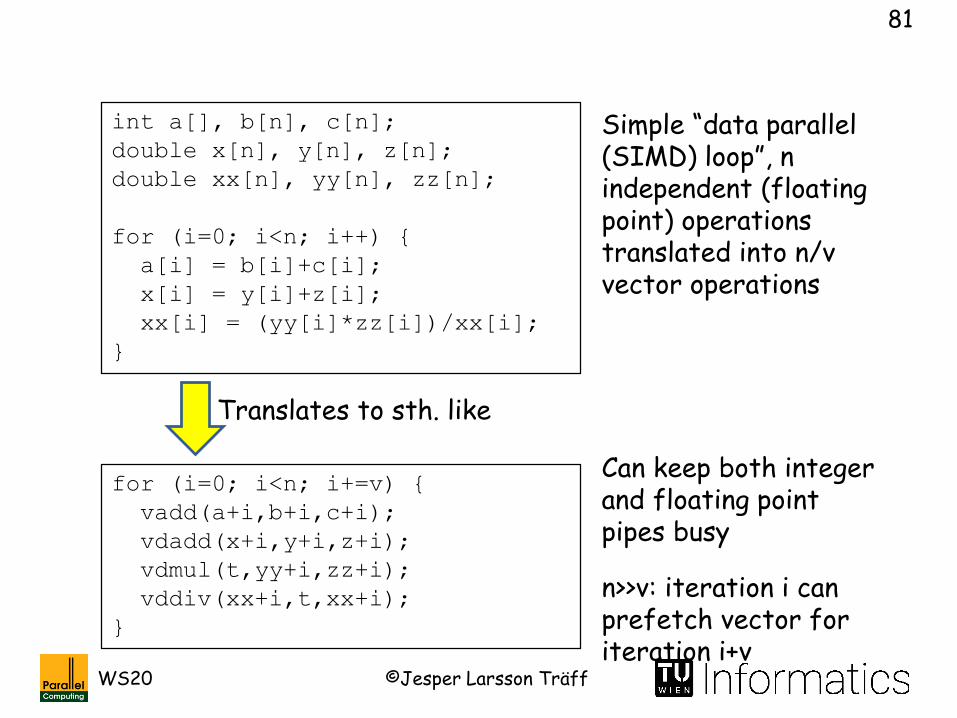
int a[], b[n], c[n];
double x[n], y[n], z[n];
double xx[n], yy[n], zz[n];
for (i=0; i<n; i++) {
a[i] = b[i]+c[i];
x[i] = y[i]+z[i];
xx[i] = (yy[i]*zz[i])/xx[i];
}
for (i=0; i<n; i+=v) {
vadd(a+i,b+i,c+i);
vdadd(x+i,y+i,z+i);
vdmul(t,yy+i,zz+i);
vddiv(xx+i,t,xx+i);
}
Simple “data parallel (SIMD) loop”, n independent (floating point) operations translated into n/v vector operations
Translates to sth. like
Can keep both integer and floating point pipes busy
n>>v: iteration i can prefetch vector for iteration i+v
©Jesper Larsson TräffWS20
83
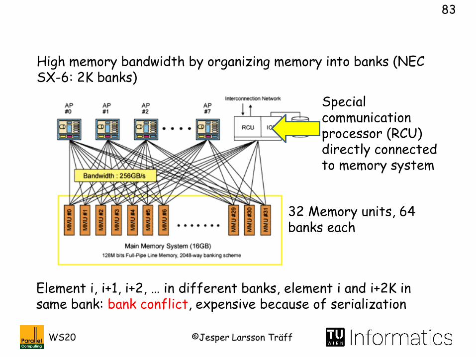
High memory bandwidth by organizing memory into banks (NEC SX-6: 2K banks)
Element i, i+1, i+2, … in different banks, element i and i+2K in same bank: bank conflict, expensive because of serialization
32 Memory units, 64 banks each
Special communication processor (RCU) directly connected to memory system
©Jesper Larsson TräffWS20
84
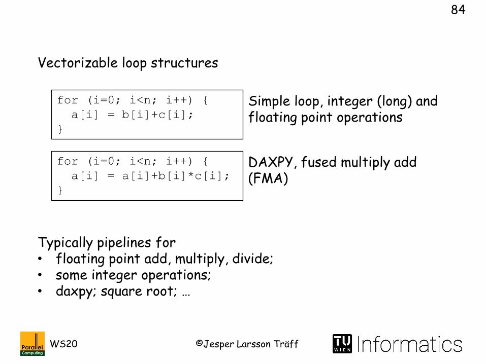
Vectorizable loop structures
for (i=0; i<n; i++) {
a[i] = b[i]+c[i];
}
for (i=0; i<n; i++) {
a[i] = a[i]+b[i]*c[i];
}
DAXPY, fused multiply add (FMA)
Simple loop, integer (long) and floating point operations
Typically pipelines for • floating point add, multiply, divide; • some integer operations; • daxpy; square root; …

©Jesper Larsson TräffWS20
85
Vectorizable loop structures
for (i=0; i<n; i++) {
if (cond[i]) a[i] = b[i]+c[i];
}
Conditional execution handled by masking
for (i=0; i<n; i++) {
R[i] = b[i]+c[i];
MASK[i] = cond[i];
if (MASK[i]) a[i] = R[i];
}
Roughly translates to:
MASK special register for conditional store, R temporary register
Wasteful when number of true-branches is small

©Jesper Larsson TräffWS20
86
Vectorizable loop structures
#pragma vdir vector,nodep
for (i=0; i<n; i++) {
a[ixa[i]] = b[ixb[i]]+c[ixc[i]];
}
Gather/Scatter operations.Compiler may need help
Can cause memory bank conflicts, depending on index vector (many indices to same bank: serialization)
Memory bandwidth dependent on access pattern

©Jesper Larsson TräffWS20
87
Vectorizable loop structures
#pragma vdir vector
for (i=1; i<n; i++) {
a[i] = a[i-1]+a[i];
}
min = a[0];
#pragma vdir vector
for (i=0; i<n; i++) {
if (a[i]<min) min = a[i];
}
Prefix-sums
Min/max operations
With special hardware support

©Jesper Larsson TräffWS20
88
#pragma vdir vector,nodep
for (i=0; i<n; i++) {
a[s*i] = b[s*i]+c[s*i];
}
Strided access
Can cause memory bank conflicts (some strides always bad)
Vectorizable loop structures
Large-vector processors currently out of fashion in HPC, almost non-existent
NEC SX-8 (2005), NEC SX-9 (2008), NEC SX-ACE (2013)
2009-2013: No NEC vector processors (market lost?)

©Jesper Larsson TräffWS20
89
NEC SX-Aurora TSUBASA: Vector Engine (ca. 2017)
• 8-core vector processor
• 1.2 TBytes/Second memory bandwidth Rpeak: 2.45TFLOPS
©Jesper Larsson TräffWS20
90
Many scientific applications fit well with vector model. Irregular, non-numerical applications often not
Mature compiler technology for vectorization and optimization(loop splitting, loop fusion…). Aim: Keep vector pipes busy
Allen, Kennedy: “Optimizing Compilers for Modern Architectures”, MKP 2002
Scalar (non-vectorizable) code carried out by standard, scalar processor; amount limits performance (Amdahl’s Law)
Vector programming model: Loops, sequential control flow, compiler handles parallelism (implicit) by vectorizing loops (some help from programmer)

©Jesper Larsson TräffWS20
91
Small scale vectorization: Standard processors
• MMX, SSE, AVX, AVX2,… (128 bit vectors, 256 bit vectors)
• Intel MIC/Xeon Phi: 512 bit vectors, new, special vector instructions (2013: Compiler support not yet mature; 2016: Much better), AVX-512 (2018: Xeon Phi defunct!)
High performance on standard processors:• Exploit vectorization potential• Check whether loops where indeed vectorized (gcc –ftree-
vectorizer-verbose=n …, in combination with architecture specific optimizations)
• Intrinsics
2, 4, 8 Floating Point operations simultaneously by one vector instruction (no integers?)

©Jesper Larsson TräffWS20
92
Support for vectorization in OpenMP 3.0
#pragma omp simd [clauses…]
for (i=0; i<n; i++) {
a[i] = b[i]+c[i];
}
Clauses: reduction (for sums), collapse (for nested loops)
©Jesper Larsson TräffWS20
93
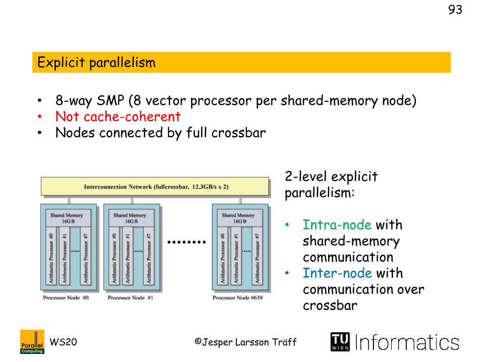
Explicit parallelism
• 8-way SMP (8 vector processor per shared-memory node)• Not cache-coherent• Nodes connected by full crossbar
2-level explicit parallelism:
• Intra-node with shared-memory communication
• Inter-node with communication over crossbar
©Jesper Larsson TräffWS20
94
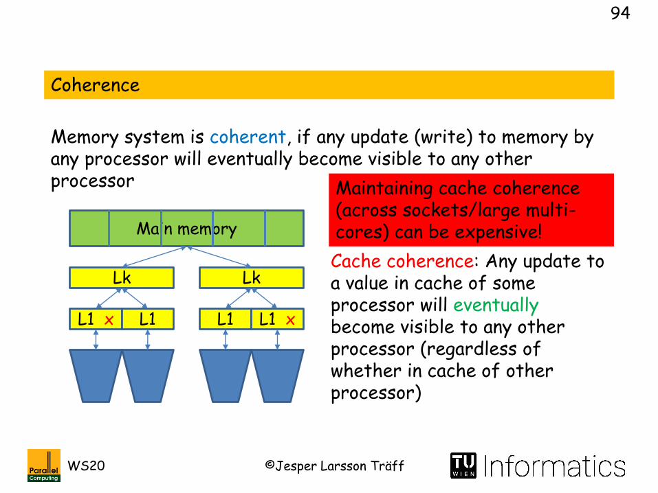
Coherence
Memory system is coherent, if any update (write) to memory by any processor will eventually become visible to any other processor
L1 x
Lk
Main memory
L1 L1
Lk
L1 x
Cache coherence: Any update to a value in cache of some processor will eventuallybecome visible to any other processor (regardless of whether in cache of other processor)
Maintaining cache coherence (across sockets/large multi-cores) can be expensive!

©Jesper Larsson TräffWS20
95
Memory behavior, memory model
• Access (read, write) to different locations may take different time (NUMA: memory network, placement of memory controllers, caches, write buffers)
• In which order will updates to different locations by some processor become visible to other processors?
• Memory model specifies: Which accesses can overtake which other accesses
Sequential consistency: Accesses take effect in program order
Most modern processors are not sequentially consistent

©Jesper Larsson TräffWS20
96
No cache-coherence: Earth Simulator/NEC SX
• Scalar unit of vector processor has cache• Caches of different processors not coherent• Vector units read/write directly to memory, no vector caches• Write-through cache
Different design choice:Cray X1 (vector computer early 2000) had a different, cache-coherent design
• Nodes must coordinate and synchronize• Parallel programming model (OpenMP, MPI) helps
D. Abts, S. Scott, D. J. Lilja: “So Many States, So Little Time: Verifying Memory Coherence in the Cray X1”, IPDPS 2003: 11

©Jesper Larsson TräffWS20
97
Example: MPI and cache non-coherence
i j
MPI_Recv(&y,…,comm,&status);
MPI_Send(&x,…,comm);
x: Mem of rank i y: Mem of rank j
y: Cache of j
Coherency/consistency needed after MPI_Recv: rank j must invalidate cache(lines) at the point where MPI requires coherence (at MPI_Recv)
Incoherent state
Processes i and j on same node
Vectorized memcpy
write
©Jesper Larsson TräffWS20
98
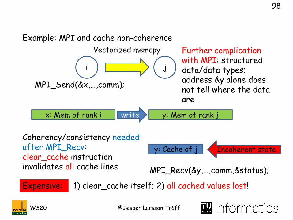
Example: MPI and cache non-coherence
i j
MPI_Recv(&y,…,comm,&status);
MPI_Send(&x,…,comm);
x: Mem of rank i y: Mem of rank j
y: Cache of j
Coherency/consistency needed after MPI_Recv:clear_cache instruction invalidates all cache lines
Incoherent state
Expensive: 1) clear_cache itself; 2) all cached values lost!
Further complication with MPI: structured data/data types; address &y alone does not tell where the data are
Vectorized memcpy
write
©Jesper Larsson TräffWS20
99
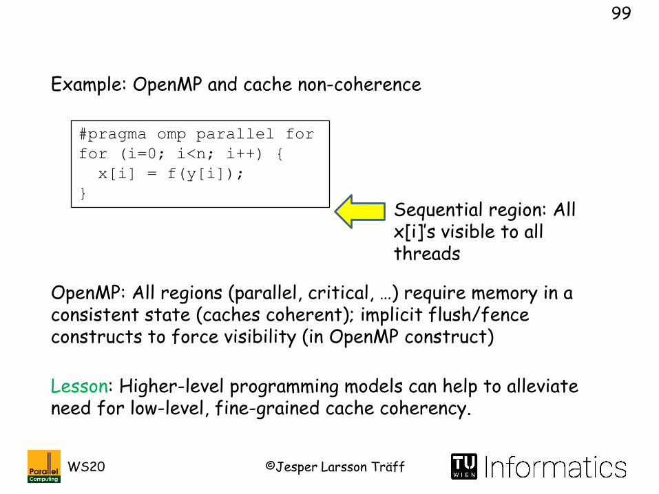
Example: OpenMP and cache non-coherence
#pragma omp parallel for
for (i=0; i<n; i++) {
x[i] = f(y[i]);
}
Sequential region: All x[i]’s visible to all threads
OpenMP: All regions (parallel, critical, …) require memory in a consistent state (caches coherent); implicit flush/fence constructs to force visibility (in OpenMP construct)
Lesson: Higher-level programming models can help to alleviate need for low-level, fine-grained cache coherency.

©Jesper Larsson TräffWS20
100
Cache coherence debate
• Cache: Beneficial for applications with spatial and/or temporal locality (not all applications have this: Graph algorithms)
• Caches a major factor in single-processor performance increase (since sometime in the 80ties)
Many new challenges for caches in parallel processors:• Coherency• Scalability• Resource consumption (logic=transistors=chip area; energy)• …
Milo M. K. Martin, Mark D. Hill, Daniel J. Sorin: Why on-chip cache coherence is here to stay. Commun. ACM 55(7): 78-89 (2012)
Too expensive?
©Jesper Larsson TräffWS20
101
MPI and OpenMP
Still most widely used programming interfaces/models for parallel HPC (there are contenders)
MPI: Message-Passing Interface, see www.mpi-forum.org
• MPI processes (ranks) communicate explicitly: point-to-point-communication, one-sided communication, collective communication, parallel I/O
• Subgrouping and encapsulation (communicators)• Much support functionality
OpenMP: shared-memory interface (C/Fortran pragma-extension), data (loops) and task parallel support, see www.openmp.org

©Jesper Larsson TräffWS20
102
Partitioned Global Address Space (PGAS) alternative to MPI
Addressing mechanism for part of the processor-local address space can be shared between processes; referencing non-local parts of partitioned space leads to implicit communication
Language or library supported:Some data structures (typically arrays) can be declared as shared (partitioned) across (all) threads
Note:PGAS not same as Distributed Shared Memory (DSM). PGAS explicitly controls which data structures (arrays) are partitioned, and how they are partitioned

©Jesper Larsson TräffWS20
103
Global array(s):
Thread k owns
a:
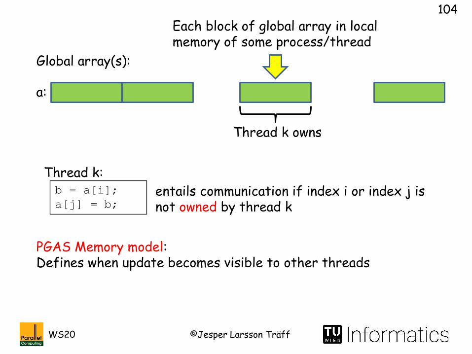
Each block of global array in local memory of some process/thread
Simple, block cyclic distribution of array a
PGAS:Data structures (simple arrays) partitioned (shared) over the memory of p threads
©Jesper Larsson TräffWS20
104
Global array(s):
Thread k owns
b = a[i];
a[j] = b;
Thread k:
PGAS Memory model:Defines when update becomes visible to other threads
entails communication if index i or index j is not owned by thread k
a:
Each block of global array in local memory of some process/thread

©Jesper Larsson TräffWS20
105
Global array(s):
a[i] = b[j];
Thread k:
even if neither a[i] nor b[j] owned by k
Thread k owns
PGAS Memory model:Defines when update becomes visible to other threads
a:
©Jesper Larsson TräffWS20
106
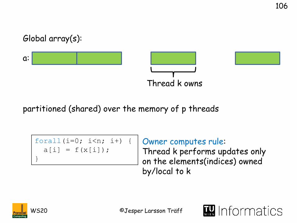
Global array(s):
forall(i=0; i<n; i+) {
a[i] = f(x[i]);
}
Owner computes rule:Thread k performs updates only on the elements(indices) owned by/local to k
partitioned (shared) over the memory of p threads
Thread k owns
a:

©Jesper Larsson TräffWS20
107
Typical PGAS features:
Even more extreme:SIMD array languages, array operations parallelized by library and runtime
Often less support for library building (process subgoups) than MPI
• Array assignments/operations translated into communication when necessary based on ownership
• Mostly simple, block-cyclic distributions of (multi-dimensional) arrays
• Collective communication support for redistribution, collective data transfer (transpositions, gather/scatter) and reduction-type operations
• Bulk-operations, array operations

©Jesper Larsson TräffWS20
108
Some PGAS languages/interfaces:
• UPC/UPC++: Unified Parallel C, C/C++ language extension; collective communication support; severe limitations
• CaF: Co-array Fortran, standardized, but limited PGAS extension to Fortran
• CAF2: considerably more powerful, non-standardized Fortran extension
• X10 (Habanero): IBM asynchronous PGAS language• Chapel: Cray, powerful data structure support• Titanium: Java-extension
• Global Arrays (GA): older, PGAS-like library for array programming , see http://hpc.pnl.gov/globalarrays/
• HPF: High-Performance Fortran
Fortran is still an important language in HPC

©Jesper Larsson TräffWS20
109
Mattias De Wael, Stefan Marr, Bruno De Fraine, Tom Van Cutsem, Wolfgang De Meuter: Partitioned Global Address Space Languages. ACM Comput. Surv. 47(4): 62:1-62:27 (2015)
Activity, maturity of PGAS languages?
UPC finds some applications
Martina Prugger, Lukas Einkemmer, Alexander Ostermann: Evaluation of the partitioned global address space (PGAS) model for an inviscid Euler solver. Parallel Computing 60: 22-40 (2016)
No new developments for the past decade? Implementation status and performance not discussed. Many PGAS language implementations use MPI as (default) communication layer
©Jesper Larsson TräffWS20
110
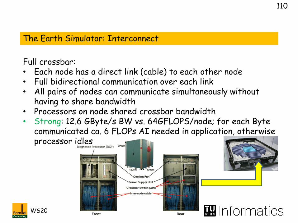
The Earth Simulator: Interconnect
Full crossbar:• Each node has a direct link (cable) to each other node• Full bidirectional communication over each link• All pairs of nodes can communicate simultaneously without
having to share bandwidth• Processors on node shared crossbar bandwidth• Strong: 12.6 GByte/s BW vs. 64GFLOPS/node; for each Byte
communicated ca. 6 FLOPs AI needed in application, otherwise processor idles

©Jesper Larsson TräffWS20
111
Fully connected network, p nodes, floor(p/2) possible pairs, in all pairings all nodes can communicate directly
Maximum distance between any two nodes (diameter): one link
P N NNN
P N NNN
P N NNN
P N NNN
Fully connected network realized as (indirect) crossbar network

©Jesper Larsson TräffWS20
112
Hierarchical/Hybrid communication subsystems
• Processors placed in shared-memory nodes; processors on same node are “closer” than processors on different nodes
• Different communication media within nodes (e.g., shared-memory) and between nodes (e.g., crossbar network)
• Processors on same node share bandwidth of inter-node network
• Compute nodes may have one or more “lanes” (rails) to network(s)
M
P P P P
M
P P P P
M
P P P P
M
P P P P
Communication network

©Jesper Larsson TräffWS20
113
M
P P P P
M
P P P P
M
P P P P
M
P P P P
Communication network
Actually, many more hierarchy levels:• Cache (and memory) hierarchy:
L1 (data/instruction) -> L2 –> L3 (…)• Processors (multi-core) share caches at certain levels
(processor may differ, e.g., AMD vs. Intel)• Network may itself be hierarchical (Clos/fat tree:
InfiniBand): Nodes, Racks, Islands, …

©Jesper Larsson TräffWS20
114
Part 1
Hierarchical communication system
Processors can be partitioned (non-trivially) such that:• Processors in same partition communicate with roughly same
performance (latency, bandwidth, number of ports, …)• Processors in different partitions communicate with roughly
same (lower) performance
Part 0 Part 1 Part k
Processors
…
Can again be hierarchical
A crossbar network is nothierarchical (all processors can communicate with same performance

©Jesper Larsson TräffWS20
115
“Pure”, homogeneous programming models oblivious to hierarchy• MPI (no performance model, only indirect mechanisms for
grouping processes according to system structure: MPI topologies)
• UPC (local/global, no grouping at all)• …
Implementation challenge for compiler/library implementer to take hierarchy into account:• Point-to-point communication uses closest path, e.g., shared
memory when possible• Efficient, hierarchical collective communication algorithms
exist (for some cases, still incomplete and immature)
Programming model and system hierarchy
©Jesper Larsson TräffWS20
116
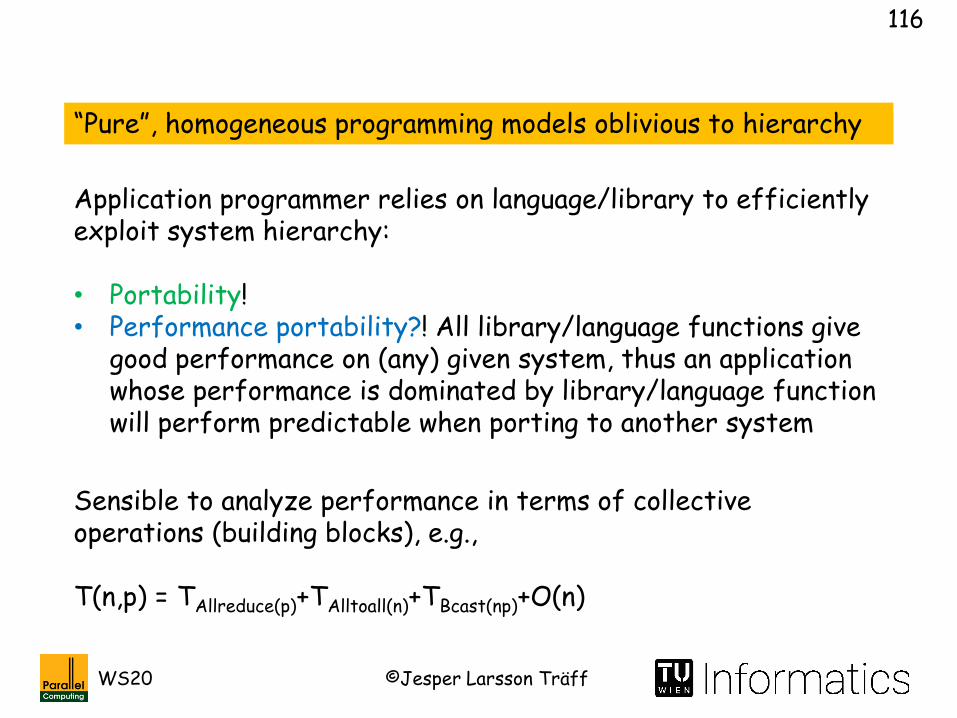
“Pure”, homogeneous programming models oblivious to hierarchy
Application programmer relies on language/library to efficiently exploit system hierarchy:
• Portability!• Performance portability?! All library/language functions give
good performance on (any) given system, thus an application whose performance is dominated by library/language function will perform predictable when porting to another system
Sensible to analyze performance in terms of collective operations (building blocks), e.g.,
T(n,p) = TAllreduce(p)+TAlltoall(n)+TBcast(np)+O(n)

©Jesper Larsson TräffWS20
117
Hybrid/heterogeneous programming models (“MPI+X”)
• Conscious to certain aspects/levels of hierarchy• Possibly more efficient application code:
• Example: MPI+OpenMP
• Less portable, less performance portable• Sometimes unavoidable (accelerators): OpenCL, OpenMP,
OpenACC, …
M
P P P P
M
P P P P
M
P P P P
M
P P P P
Communication network
OpenMP
MPI between master threads

©Jesper Larsson TräffWS20
118
Earth simulator 2/SX-9, 2009
Compared to SX-6/Earth Simulator:• More pipes• Special pipes (square root)
Peak performance >100GFLOPS/processor

©Jesper Larsson TräffWS20
119
Peak performance/CPU
102.4GflopsTotal number of CPUs
1280
Peak performance/PN
819.2GflopsTotal number of PNs
160
Shared memory/PN
128GByteTotal peak performance
131Tflops
CPUs/PN 8 Total main memory
20TByte
Earth Simulator 2/SX-9 system

©Jesper Larsson TräffWS20
120
Cheaper communication network than full crossbar: Fat-Tree
©Jesper Larsson TräffWS20
121
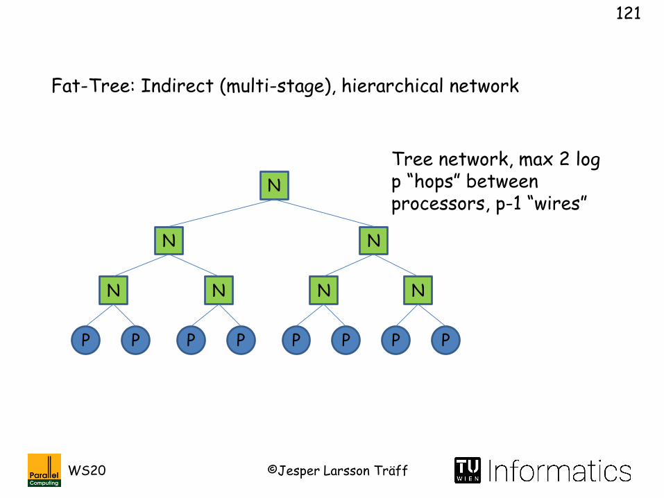
Fat-Tree: Indirect (multi-stage), hierarchical network
P P
N
P P
N
P P
N
P P
N
N N
N
Tree network, max 2 log p “hops” between processors, p-1 “wires”

©Jesper Larsson TräffWS20
122
P P
N
P P
N
P P
N
P P
N
N N
N
Bandwidth increases, “fatter” wires
C. E. Leiserson: Fat-Trees: Universal Networks for Hardware-Efficient Supercomputing. IEEE Trans. Computers 34(10): 892-901, 1985
Fat-Tree: Indirect (multi-stage), hierarchical network

©Jesper Larsson TräffWS20
123
P P
N
P P
N
P P
N
P P
N
N N
N
C. E. Leiserson: Fat-Trees: Universal Networks for Hardware-Efficient Supercomputing. IEEE Trans. Computers 34(10): 892-901, 1985
Thinking Machines CM5, on first, unofficial Top500
Fat-Tree: Indirect (multi-stage), hierarchical network

©Jesper Larsson TräffWS20
124
P P
N
P P
N
P P
N
P P
N
N NN N N
N
N
NN N NN Realization with N small crossbar switches
Fat-Tree: Indirect (multi-stage), hierarchical network
Example: InfiniBand
©Jesper Larsson TräffWS20
125
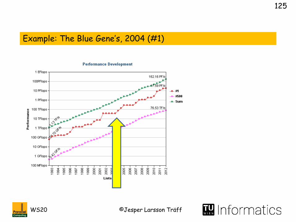
Example: The Blue Gene’s, 2004 (#1)
©Jesper Larsson TräffWS20
126
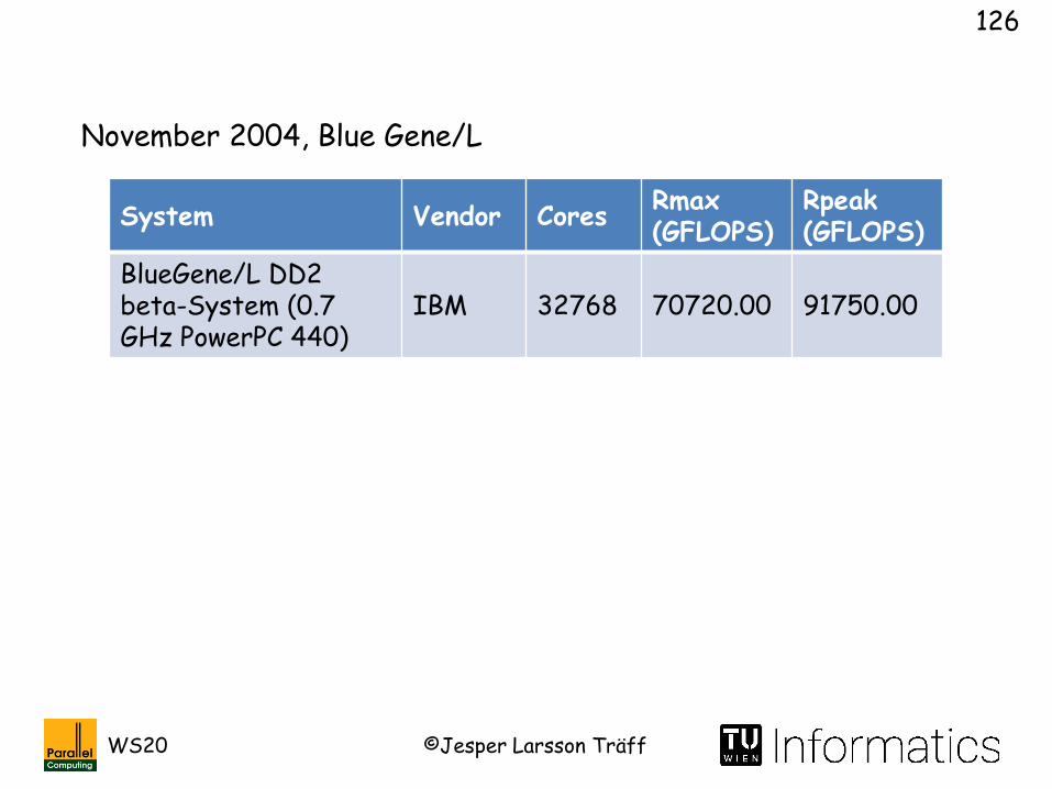
System Vendor CoresRmax(GFLOPS)
Rpeak(GFLOPS)
BlueGene/L DD2 beta-System (0.7 GHz PowerPC 440)
IBM 32768 70720.00 91750.00
November 2004, Blue Gene/L
©Jesper Larsson TräffWS20
127
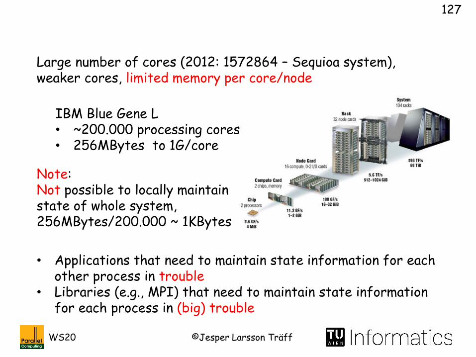
Large number of cores (2012: 1572864 – Sequioa system), weaker cores, limited memory per core/node
IBM Blue Gene L• ~200.000 processing cores• 256MBytes to 1G/core
Note:Not possible to locally maintain state of whole system, 256MBytes/200.000 ~ 1KBytes
• Applications that need to maintain state information for each other process in trouble
• Libraries (e.g., MPI) that need to maintain state information for each process in (big) trouble
©Jesper Larsson TräffWS20
128
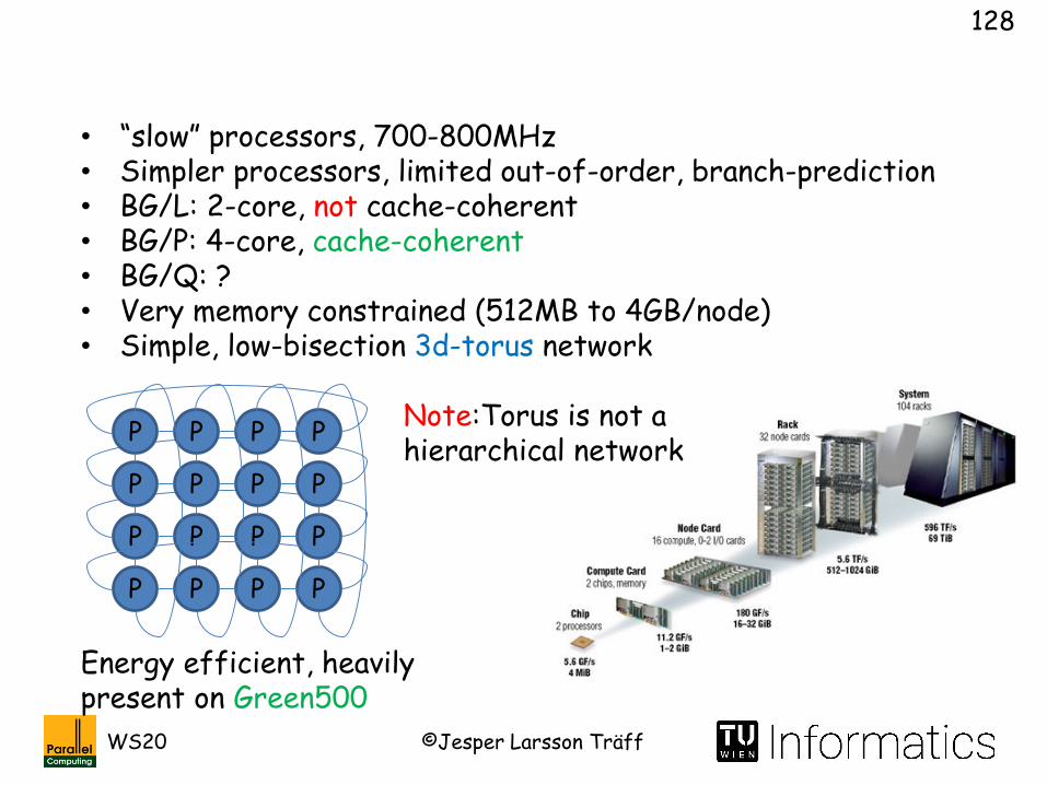
• “slow” processors, 700-800MHz• Simpler processors, limited out-of-order, branch-prediction• BG/L: 2-core, not cache-coherent• BG/P: 4-core, cache-coherent• BG/Q: ?• Very memory constrained (512MB to 4GB/node)• Simple, low-bisection 3d-torus network
Energy efficient, heavily present on Green500
P P P P
P P P P
P P P P
P P P P
Note:Torus is not a hierarchical network

©Jesper Larsson TräffWS20
129
José E. Moreira, Valentina Salapura, George Almási, Charles Archer, Ralph Bellofatto, Peter Bergner, Randy Bickford, Matthias A. Blumrich, José R. Brunheroto, Arthur A. Bright, Michael Brutman, José G. Castaños, Dong Chen, Paul Coteus, Paul Crumley, Sam Ellis, Thomas Engelsiepen, Alan Gara, Mark Giampapa, Tom Gooding, Shawn Hall, Ruud A. Haring, Roger L. Haskin, Philip Heidelberger, Dirk Hoenicke, Todd Inglett, Gerard V. Kopcsay, Derek Lieber, David Limpert, Patrick McCarthy, Mark Megerian, Michael Mundy, Martin Ohmacht, Jeff Parker, Rick A. Rand, Don Reed, Ramendra K. Sahoo, Alda Sanomiya, Richard Shok, Brian E. Smith, Gordon G. Stewart, Todd Takken, PavlosVranas, Brian P. Wallenfelt, Michael Blocksome, Joe Ratterman: The Blue Gene/L Supercomputer: A Hardware and Software Story. International Journal of Parallel Programming 35(3): 181-206 (2007)
On the BlueGene/L System

©Jesper Larsson TräffWS20
130
George Almási, Charles Archer, José G. Castaños, John A. Gunnels, C. Christopher Erway, Philip Heidelberger, Xavier Martorell, José E. Moreira, Kurt W. Pinnow, Joe Ratterman, Burkhard D. Steinmacher-Burow, William Gropp, Brian R. Toonen:Design and implementation of message-passing services for the Blue Gene/L supercomputer. IBM Journal of Research and Development 49(2-3): 393-406 (2005)
On MPI for the BlueGene/L System
©Jesper Larsson TräffWS20
131
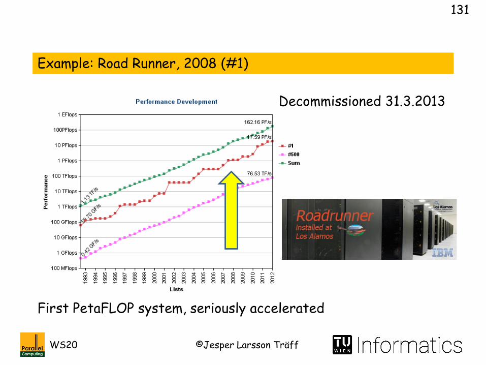
Example: Road Runner, 2008 (#1)
First PetaFLOP system, seriously accelerated
Decommissioned 31.3.2013

©Jesper Larsson TräffWS20
132
System Vendor CoresRmax(TF)
Rpeak(TF)
Power(KW)
BladeCenter QS22/LS21 Cluster, PowerXCell 8i 3.2 Ghz / Opteron DC 1.8 GHz, Voltaire InfiniBand
IBM 129600 1105.0 1456.7 2483.00
November 2008, Road Runner
What counts as a “core”?
©Jesper Larsson TräffWS20
133
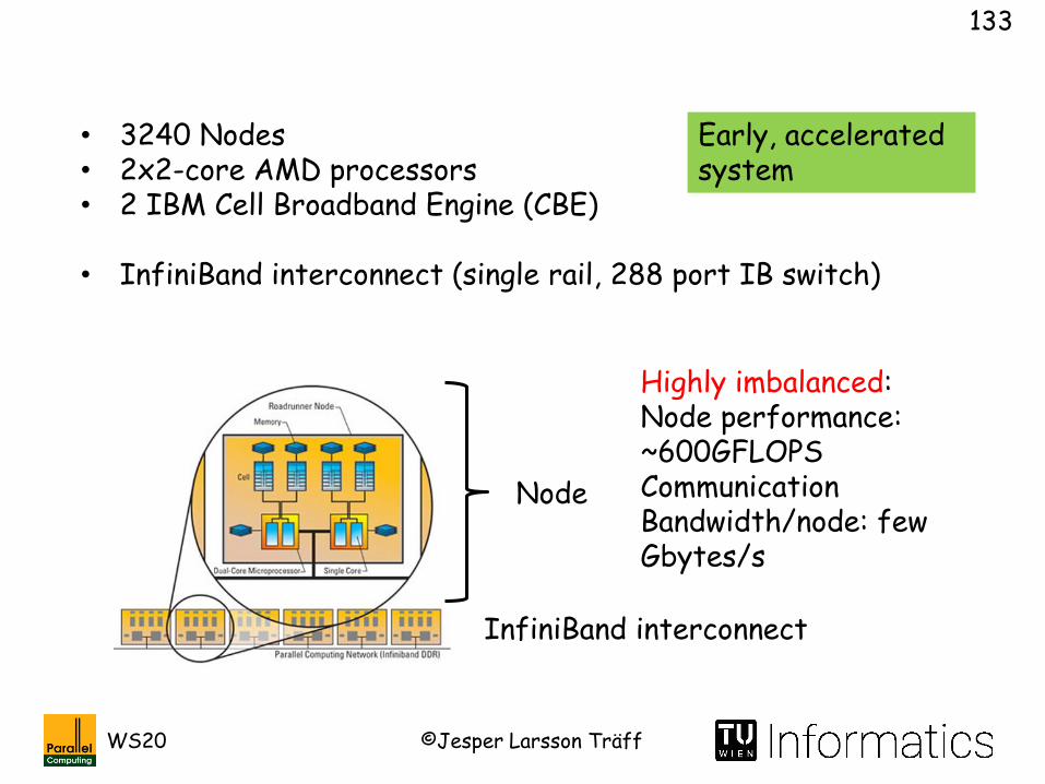
• 3240 Nodes• 2x2-core AMD processors • 2 IBM Cell Broadband Engine (CBE)
• InfiniBand interconnect (single rail, 288 port IB switch)
Node
InfiniBand interconnect
Highly imbalanced:Node performance: ~600GFLOPS Communication Bandwidth/node: few Gbytes/s
Early, accelerated system

©Jesper Larsson TräffWS20
134
25,6GByte/sTotal BW>300GByte/s
Standard IBM scalar PowerPC architecture
Multiple ring network with atomic operations
~total 250GFLOPS

©Jesper Larsson TräffWS20
135
25.6 GFLOPS (32-bit!)
• SIMD (128-bit vectors, 4 32-bit words)
• Single-issue, no out-of-order capabilities, limited (no?) branch prediction
Small local storage, 256KB, no cache (no coherency)

©Jesper Larsson TräffWS20
136
Complex, heterogeneous system: Complex programming model (?)
• Deeply hierarchical system: SPE’s -> PPE -> Multi-core -> InfiniBand
• MPI communication between multi-core nodes, either all processors per node or one process per node
• Possibly OpenMP/shared memory model on nodes• Offload to CBE of compute-intensive kernels• CBE programming: PPE/SPE, vectorization, explicit
communication between SPE’s, PPE, node-memory
Road Runner requires very (very) compute intensive applications
Extremely high AI (arithmetic/operational intensity) needed to exploit this system

©Jesper Larsson TräffWS20
137
MPI communication
• Let the SPEs of the Cell be full-fledged MPI processes• Offload to CPUs as needed/possible
Pakin et al.: The reverse-acceleration model for programming petascale hybrid systems. IBM J. Res. And Dev, (5): 8, 2009
Drawbacks:• Latency high (SPE -> PPE -> CPU -> IB)• Supports only subset of MPI
©Jesper Larsson TräffWS20
138
M
P P P P
M
P P P P
M
P P P P
M
P P P P
Communication network
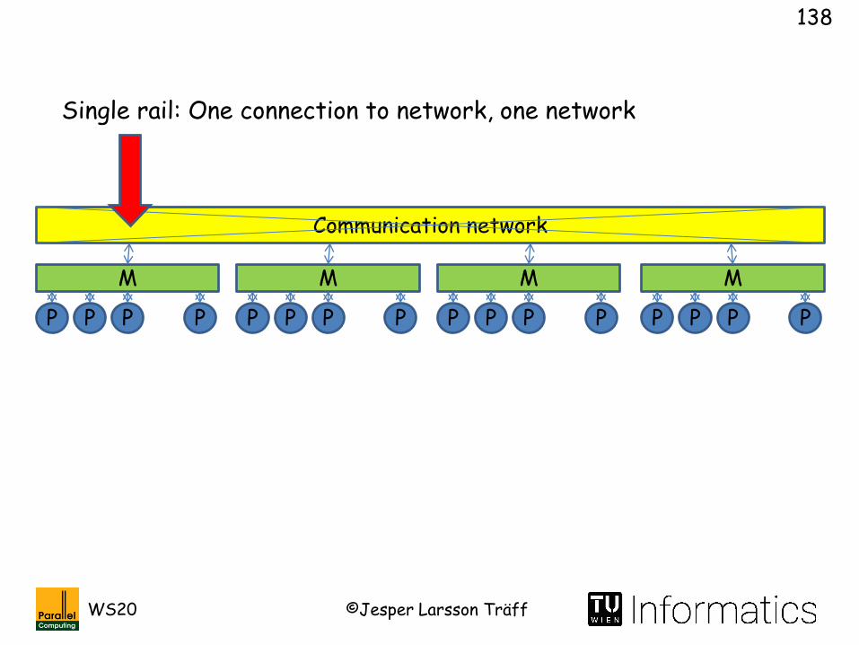
Single rail: One connection to network, one network

©Jesper Larsson TräffWS20
139
M
P P P P
M
P P P P
M
P P P P
M
P P P P
Communication network
Communication bandwidth can be improved by providing more lanes (rails) to network, and more duplicates of network (multi-rail). Network costs increase proportionally
Examples:• VSC-3 (2014)• Summit, Sierra (2018)
Top500 exercise: Which was the first multi-rail system? When?

©Jesper Larsson TräffWS20
140
• “LIMIEUX”, Pittsburg Supercomputing Center, 2001-2006, dual rail Quadrics https://www.psc.edu/news-publications/30-years-of-psc (Top500 #2, Nov. 2001)
• “Pleiades”, NASA Ames, some nodes with multi-ported InfiniBand (Top500 #11, Nov. 2008)
• “TSUBAME 2.0”, some nodes with 2xInfiniBand (Top500 #4, Nov. 2010)
”Solution” to exercise, information not in Top500
Thanks to Anton Görgl, WS 2019
©Jesper Larsson TräffWS20
141
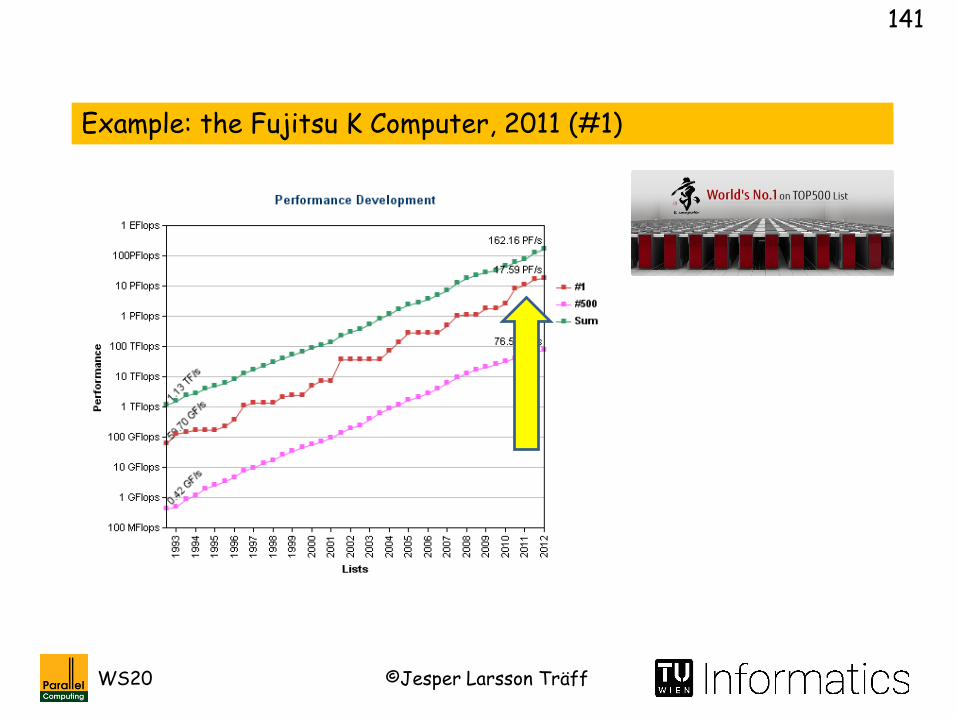
Example: the Fujitsu K Computer, 2011 (#1)

©Jesper Larsson TräffWS20
142
System Vendor CoresRmax(TF)
Rpeak(TF)
Power(KW)
K computer, SPARC64 VIIIfx 2.0GHz, Tofu interconnect
Fujitsu 548352 8162.0 8773.6 9898.56
June 2011, K-Computer

©Jesper Larsson TräffWS20
143
• High-end, multithreaded, scalar processor (SPARC64 VIIIfx)• Many special instructions• 16GFLOPS per core (Rpeak/#cores)
• 6-dimensional torus
• Homogeneous, no accelerator!
Yuichiro Ajima, Tomohiro Inoue, Shinya Hiramoto, Yuzo Takagi, Toshiyuki Shimizu: The Tofu Interconnect. IEEE Micro 32(1): 21-31 (2012)Yuichiro Ajima, Shinji Sumimoto, Toshiyuki Shimizu: Tofu: A 6D Mesh/Torus Interconnect for Exascale Computers. IEEE Computer 42(11): 36-40 (2009)
©Jesper Larsson TräffWS20
144
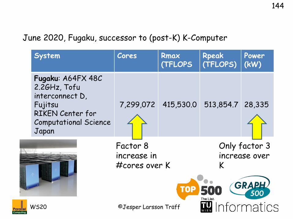
June 2020, Fugaku, successor to (post-K) K-Computer
System Cores Rmax(TFLOPS
Rpeak(TFLOPS)
Power(kW)
Fugaku: A64FX 48C 2.2GHz, Tofu interconnect D, Fujitsu RIKEN Center for Computational ScienceJapan
7,299,072 415,530.0 513,854.7 28,335
Factor 8 increase in #cores over K
Only factor 3increase over K
©Jesper Larsson TräffWS20
145
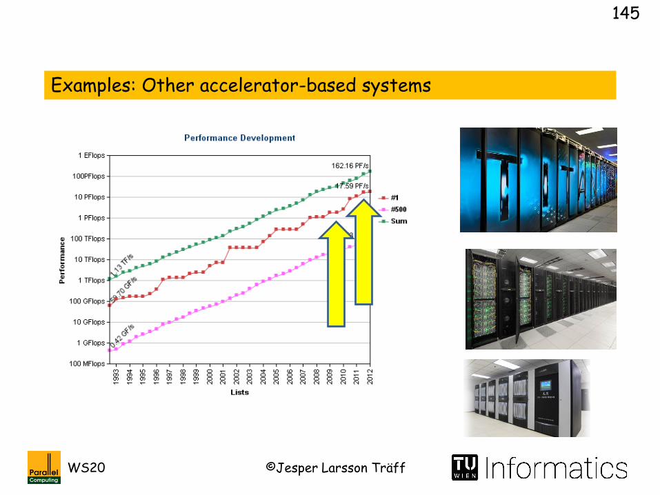
Examples: Other accelerator-based systems
©Jesper Larsson TräffWS20
146
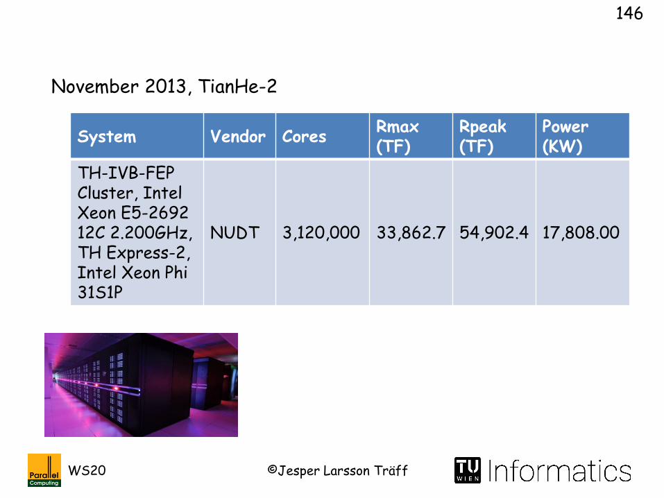
November 2013, TianHe-2
System Vendor CoresRmax(TF)
Rpeak(TF)
Power(KW)
TH-IVB-FEP Cluster, Intel Xeon E5-2692 12C 2.200GHz, TH Express-2, Intel Xeon Phi 31S1P
NUDT 3,120,000 33,862.7 54,902.4 17,808.00

©Jesper Larsson TräffWS20
147
June 2019: Rank #1: NVidia GPU
System CoresRmax(TFLOPS)
Rpeak(TFLOPS)
Power (kW)
Summit: IBM Power System AC922, IBM POWER9 22C 3.07GHz, NVIDIA Volta GV100, Dual-rail MellanoxEDR Infiniband , IBM DOE/SC/Oak Ridge National LaboratoryUnited States
2,414,592 148,600.0 200,794.9 10,096

©Jesper Larsson TräffWS20
148
System Vendor CoresRmax(TF)
Rpeak(TF)
Power(KW)
Cray XK7,Opteron 6274 16C 2.200GHz, Cray Gemini interconnect, NVIDIA K20x
Cray 560640 17590.0 27112.5 8209.00
November 2012, Cray Titan: NVidia GPU

©Jesper Larsson TräffWS20
149
System Vendor Cores Rmax RpeakPower (KW)
PowerEdgeC8220, Xeon E5-2680 8C 2.700GHz, InfinibandFDR, Intel Xeon Phi
Dell 462462 5,168.1 8,520.1 4,510.00
November 2012, Stampede (#7): Intel Xeon Phi

©Jesper Larsson TräffWS20
150
System Vendor Cores Rmax Rpeak Power
NUDT TH MPP, X5670 2.93Ghz 6C, NVIDIA GPU, FT-1000 8C
NUDT 186368 2566.0 4701.0 4040.00
November 2010, Tianhe: NVidia GPU

©Jesper Larsson TräffWS20
151
Hybrid architectures with accelerator support (GPU, MIC)
• High-performance and low energy consumption through accelerators
• GPU accelerator: Highly parallel “throughput architecture”, lightweight cores, complex memory hierarchy, banked memory
• MIC accelerator: Lightweight x86 cores, extended vectorization, ring-network on chip

©Jesper Larsson TräffWS20
152
Hybrid architectures with accelerator support (GPU, MIC)
Issues with accelerator: currently (2013) limited on-chip memory (MIC 8GByte), PCIex connection to main processor
Programming: Kernel offload, explicitly with OpenCL/CUDA
MIC: Some “reverse acceleration” projects, MPI between MIC cores

©Jesper Larsson TräffWS20
153
Main memory
Lk
L1
SIMD
Acc
Heavily accelerated system, one or more accelerators
Acc memory
Memory hierarchy
This will likely change
Although same ISA, heterogeneous programming model (offloading) may be needed
OpenMP, OpenACC, … (+MPI)
News late 2017: KNL… line discontinued by Intel
©Jesper Larsson TräffWS20
154
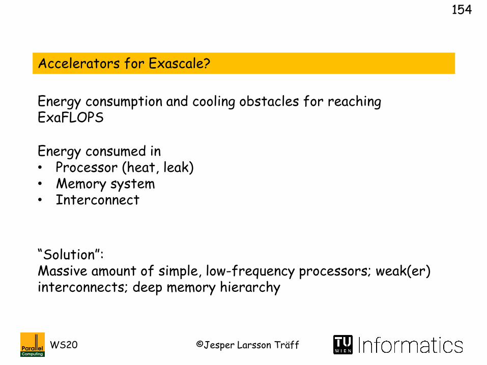
Accelerators for Exascale?
Energy consumption and cooling obstacles for reaching ExaFLOPS
Energy consumed in• Processor (heat, leak)• Memory system• Interconnect
“Solution”:Massive amount of simple, low-frequency processors; weak(er) interconnects; deep memory hierarchy

©Jesper Larsson TräffWS20
155
Run-of-the-mill
System Vendor Cores Rmax Rpeak Power
Megware Saxonid6100, Opteron 8C 2.2 GHz, InfinibandQDR
Megware 20776 152.9 182.8 430.00
VSC-2, June 2011, November 2012: #162
Similar to TU Wien, Parallel Computing group “jupiter”, our first, small cluster (NEC)

©Jesper Larsson TräffWS20
156
Run-of-the-mill
System Vendor Cores Rmax Rpeak Power
Oil blade server, Intel Xeon E5-2650v2 8C 2.6GHz, Intel TrueScaleInfiniband
ClusterVision
32,768 596.0 681.6 450.00
VSC-3 November 2014 #85; November 2015 #138; November 2016 #246; November 2017 #460
• Innovative oil cooling• Dual rail InfiniBand2020 nodes
(initial), 2x8=16 cores per node
©Jesper Larsson TräffWS20
157
Run-of-the-mill
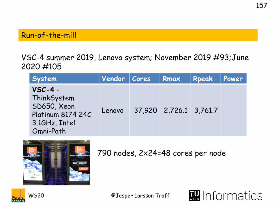
VSC-4 summer 2019, Lenovo system; November 2019 #93;June 2020 #105
System Vendor Cores Rmax Rpeak Power
VSC-4 -ThinkSystemSD650, Xeon Platinum 8174 24C 3.1GHz, Intel Omni-Path
Lenovo 37,920 2,726.1 3,761.7
790 nodes, 2x24=48 cores per node

©Jesper Larsson TräffWS20
158
Memory in HPC systems (2015)
System #Cores Memory (GB)
Memory/Core (GB)
TianHe-2 3,120,000 1,024,000 0,33
Titan (Cray XK) 560,640 710,144 1,27
Sequoia (IBM BG/Q) 1,572,864 1,572,864 1
K (Fujitsu SPARC) 705,024 1,410,048 2
Stampede (Dell) 462,462 192,192 0,42
Roadrunner (IBM) 129,600 ?
Pleiades (SGI) 51,200 51,200 1
BlueGene/L (IBM) 131,072 32,768 0,25
Earth Simulator (SX9) 1,280 20,480 16
Earth Simulator (SX6) 5,120 ~10,000 1,95

©Jesper Larsson TräffWS20
159
Memory/core in HPC systems
• What is a core (GPU SIMD core)?
• Memory a scarce resource, not possible to keep state information for all cores
• Hybrid, shared memory programming models may help to keep shared structures once/node
• Algorithms must use memory efficiently: in-place, no O(n2) representations for O(n+m) sized graphs, …
©Jesper Larsson TräffWS20
160
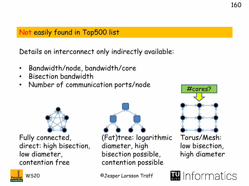
Not easily found in Top500 list
Details on interconnect only indirectly available:
• Bandwidth/node, bandwidth/core• Bisection bandwidth• Number of communication ports/node
Fully connected, direct: high bisection, low diameter, contention free
(Fat)tree: logarithmic diameter, high bisection possible, contention possible
Torus/Mesh: low bisection, high diameter
#cores?

©Jesper Larsson TräffWS20
161
Recent history (2010) :
SiCortex (2003-09): distributed memory MIMD, Kautz-network
2010: Difficult to build (and survive commercially) “best”, real parallel computers with
• Custom processors• Custom memory• Custom communication
network
©Jesper Larsson TräffWS20
162
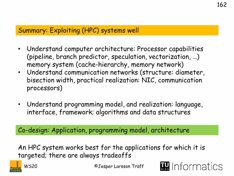
Summary: Exploiting (HPC) systems well
• Understand computer architecture: Processor capabilities (pipeline, branch predictor, speculation, vectorization, …) memory system (cache-hierarchy, memory network)
• Understand communication networks (structure: diameter, bisection width, practical realization: NIC, communication processors)
• Understand programming model, and realization: language, interface, framework; algorithms and data structures
Co-design: Application, programming model, architecture
An HPC system works best for the applications for which it is targeted; there are always tradeoffs
©Jesper Larsson TräffWS20
163
Summary: What is HPC?
Study of• Computer architecture, memory systems• Communication networks• Programming models and interfaces• (Parallel) Algorithms and data structures, for applications and
for interface support
• Assessment of computer systems: Performance models, rigorous benchmarking
For Scientific Computing (applications):• Tools, libraries, packages• (Parallel) Algorithms and data structures
©Jesper Larsson TräffWS20
164
Hennessy, Patterson: Computer Architecture – A Quantitative Approach (5 Ed.). Morgan Kaufmann, 2012
Bryant, O’Halloran: Computer Systems. Prentice-Hall, 2003
Georg Hager, Jan Treibig, Johannes Habich, Gerhard Wellein:Exploring performance and power properties of modern multi-core chips via simple machine models. Concurrency and Computation: Practice and Experience 28(2): 189-210 (2016)
Georg Hager, Gerhard Wellein: Introduction to High Performance Computing for Scientists and Engineers. Chapman and Hall / CRC computational science series, CRC Press 2011, ISBN 978-1-439-81192-4, pp. I-XXV, 1-330
Processor architecture models
Roofline model
©Jesper Larsson TräffWS20
165
Memory system
Cache system basics
Georg Hager, Gerhard Wellein: Introduction to High Performance Computing for Scientists and Engineers. Chapman and Hall / CRC computational science series, CRC Press 2011, ISBN 978-1-439-81192-4, pp. I-XXV, 1-330
• Cache-aware algorithm: Algorithm that uses memory (cache) hierarchy efficiently, under knowledge of the number of levels, cache and cache line sizes
• Cache-oblivious algorithm: Algorithm that uses memory hierarchy efficiently, without explicitly knowing cache system parameters (cache and line sizes)
• Cache-replacement strategies

©Jesper Larsson TräffWS20
166
Matteo Frigo, Charles E. Leiserson, Harald Prokop, SridharRamachandran: Cache-Oblivious Algorithms. ACM Trans. Algorithms 8(1): 4 (2012), results dating back to FOCS 1999
• Cache-aware algorithm: Algorithm that uses memory (cache) hierarchy efficiently, under knowledge of the number of levels, cache and cache line sizes
• Cache-oblivious algorithm: Algorithm that uses memory hierarchy efficiently, without explicitly knowing cache system parameters (cache and line sizes)
• Cache-replacement strategies

©Jesper Larsson TräffWS20
167
Memory system: Multi-core memory systems (NUMA)
Georg Hager, Gerhard Wellein: Introduction to High Performance Computing for Scientists and Engineers. Chapman and Hall / CRC computational science series, CRC Press 2011, ISBN 978-1-439-81192-4, pp. I-XXV, 1-330
Memory efficient algorithms: External memory model, in-place algorithms, …

©Jesper Larsson TräffWS20
168
Communication networks
• Network topologies• Routing• Modeling Some in MPI part of lecture, by need
Communication library
Efficient communication algorithms for given network assumptions inside MPI
In MPI part of lecture

©Jesper Larsson TräffWS20
169
Completely different case-study: Context allocation in MPI
Process i: MPI_Send(&x,c,MPI_INT,j,TAG, comm);
Process j: MPI_Recv(&y,c,MPI_INT,j,TAG,comm,&status);
Process j receives messages with TAG on comm in order
MPI_Send(…,j,TAG,other);no match: no communication if comm!=other
Implementation of point-to-point communication:Message envelope contains communication context, unique to comm, to distinguish messages on different communicators

©Jesper Larsson TräffWS20
170
Tradeoff: number of bits for communication context vs. number of communication contexts.Sometimes: 12 bits, 14 bits, 16 bits… (4K to 64K possible communicators)
Implementation challenges: Small envelope
Recall:• Communicators in MPI essential for safe parallel libraries,
tags not sufficient (library routines written by different people might use same tags)
• Communicators in MPI essential for algorithms that require collective communication on subsets of processes

©Jesper Larsson TräffWS20
171
MPI_Comm: MPI_COMM_WORLD
i j
MPI_Comm: local structure representing distributed communicator object
MPI_Recv(…,comm,&status);MPI_Send(…,comm);
MPI_COMM_WORLD: Default communicator, all processes
MPI_Comm_create(), MPI_Comm_split(), MPI_Dist_graph_create(), …: collective operations to create new communicators out of old ones

©Jesper Larsson TräffWS20
172
MPI_Comm_create(), MPI_Comm_split(), MPI_Dist_graph_create(), …: collective operations to create new communicators out of old ones
1. Determine which other processes will belong to new communicator
2. Allocate context id: maintain global bitmap of used id’s
Algorithm scheme, process i:
Standard implementation:
Use 4K to 64K bit vector bitmap to keep track of free communication contexts. If bitmap[i]==0, then i is a free communication context
unsigned long bitmap[words];
©Jesper Larsson TräffWS20
173
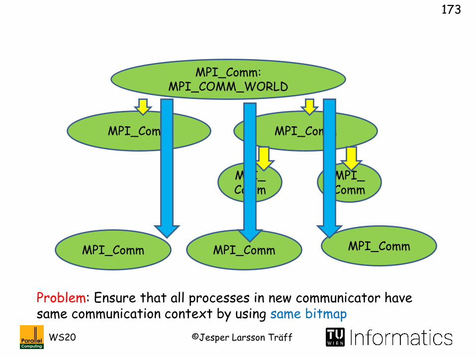
MPI_Comm: MPI_COMM_WORLD
MPI_Comm MPI_Comm
MPI_Comm
MPI_Comm
MPI_Comm MPI_CommMPI_Comm
Problem: Ensure that all processes in new communicator have same communication context by using same bitmap
©Jesper Larsson TräffWS20
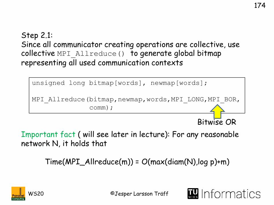
174
unsigned long bitmap[words], newmap[words];
MPI_Allreduce(bitmap,newmap,words,MPI_LONG,MPI_BOR,
comm);
Important fact ( will see later in lecture): For any reasonable network N, it holds that
Time(MPI_Allreduce(m)) = O(max(diam(N),log p)+m)
Step 2.1:Since all communicator creating operations are collective, use collective MPI_Allreduce() to generate global bitmap representing all used communication contexts
Bitwise OR

©Jesper Larsson TräffWS20
175
Typical MPI_Allreduce performance (function of problem size, fixed number of processes, p=26*16)
Time is constant for m≤K, for some small K
Use K as size of bitmap?
“jupiter” IB cluster at TU Wien“Minimum recorded time, no error bars”

©Jesper Larsson TräffWS20
176
for (i=0; i<words; i++) if (newmap[i]!=0xF…FL) break;
unsigned long x = newmap[i];
for (z=0; z<8*sizeof(x); z++)
if ((x&0x1)==0x0) break; else x>>=1;
O(words) operations
O(wordlength), dominates if words<wordlength
Step 2.2:Find first word with 0-bit
Step 2.3:Find rightmost (first) 0-bit in word
64 words of 64-bits = 4K communication contexts
Can we do better?
©Jesper Larsson TräffWS20
177
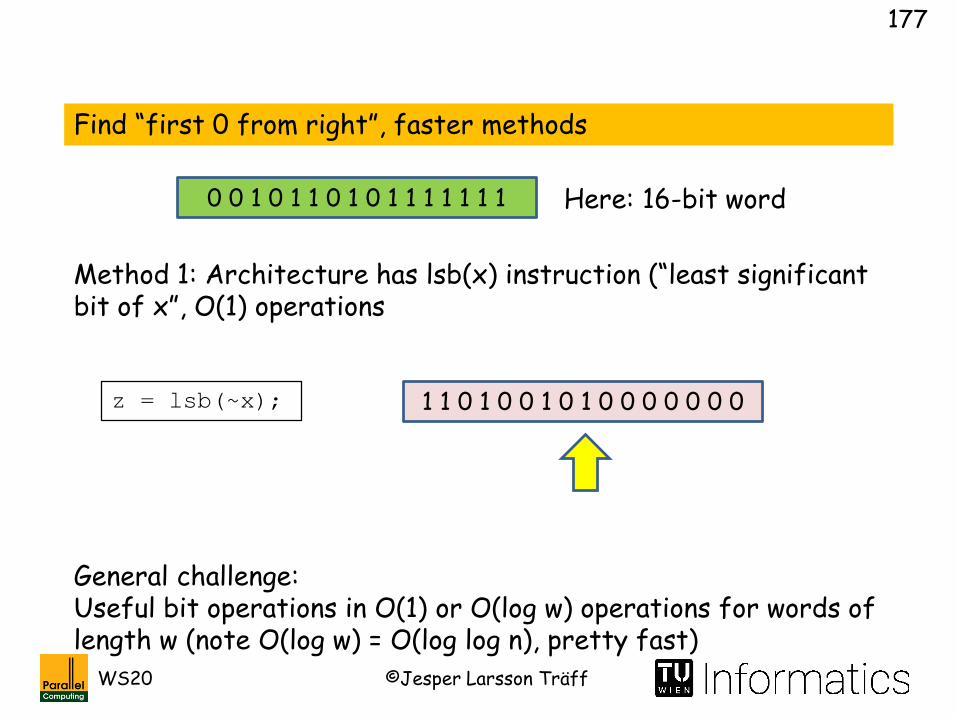
Find “first 0 from right”, faster methods
Here: 16-bit word
Method 1: Architecture has lsb(x) instruction (“least significant bit of x”, O(1) operations
z = lsb(~x);
0 0 1 0 1 1 0 1 0 1 1 1 1 1 1 1
1 1 0 1 0 0 1 0 1 0 0 0 0 0 0 0
General challenge:Useful bit operations in O(1) or O(log w) operations for words of length w (note O(log w) = O(log log n), pretty fast)

©Jesper Larsson TräffWS20
178
0 0 1 0 1 1 0 1 0 1 1 1 1 1 1 1
Method 2: Architecture has “popcount” instruction pop(x) (population count, number of 1’s in x), O(1) operations
x = x&~(x+1);
z = pop(x);0 0 1 0 1 1 0 1 1 0 0 0 0 0 0 0
1 1 0 1 0 0 1 0 0 1 1 1 1 1 1 1
0 0 0 0 0 0 0 0 0 1 1 1 1 1 1 1
z = pop(x) = 7;
Here: 16-bit word
©Jesper Larsson TräffWS20
179
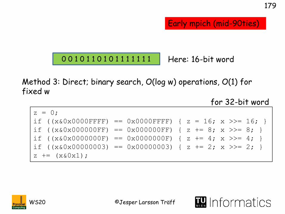
z = 0;
if ((x&0x0000FFFF) == 0x0000FFFF) { z = 16; x >>= 16; }
if ((x&0x000000FF) == 0x000000FF) { z += 8; x >>= 8; }
if ((x&0x0000000F) == 0x0000000F) { z += 4; x >>= 4; }
if ((x&0x00000003) == 0x00000003) { z += 2; x >>= 2; }
z += (x&0x1);
0 0 1 0 1 1 0 1 0 1 1 1 1 1 1 1
Method 3: Direct; binary search, O(log w) operations, O(1) for fixed w
Here: 16-bit word
for 32-bit word
Early mpich (mid-90ties)
©Jesper Larsson TräffWS20
180
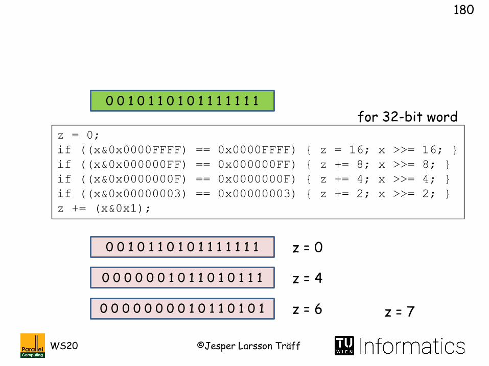
z = 0;
if ((x&0x0000FFFF) == 0x0000FFFF) { z = 16; x >>= 16; }
if ((x&0x000000FF) == 0x000000FF) { z += 8; x >>= 8; }
if ((x&0x0000000F) == 0x0000000F) { z += 4; x >>= 4; }
if ((x&0x00000003) == 0x00000003) { z += 2; x >>= 2; }
z += (x&0x1);
0 0 1 0 1 1 0 1 0 1 1 1 1 1 1 1
0 0 1 0 1 1 0 1 0 1 1 1 1 1 1 1
0 0 0 0 0 0 1 0 1 1 0 1 0 1 1 1
z = 0
z = 4
0 0 0 0 0 0 0 0 1 0 1 1 0 1 0 1 z = 6 z = 7
for 32-bit word

©Jesper Larsson TräffWS20
181
x = ~x; // invert bits
if (x==0) z = 32; else {
z = 0;
if ((x&0x0000FFFF) == 0x0) { z = 16; x >>= 16; }
if ((x&0x000000FF) == 0x0) { z += 8; x >>= 8; }
if ((x&0x0000000F) == 0x0) { z += 4; x >>= 4; }
if ((x&0x00000003) == 0x0) { z += 2; x >>= 2; }
z -= (x&0x1);
}
0 0 1 0 1 1 0 1 0 1 1 1 1 1 1 1
Method 3a: direct; binary search to find lsb
Here: 16-bit word
Might be better because masks needed only once
for 32-bit word

©Jesper Larsson TräffWS20
182
x = x&~(x+1);
x = (x&0x55555555) + ((x>>1)&0x55555555);
x = (x&0x33333333) + ((x>>2)&0x33333333);
x = (x&0x0F0F0F0F) + ((x>>4)&0x0F0F0F0F);
x = (x&0x00FF00FF) + ((x>>8)&0x00FF00FF);
x = (x&0x0000FFFF) + ((x>>16)&0x0000FFFF);
0 0 1 0 1 1 0 1 0 1 1 1 1 1 1 1
Method 4: implement popcount
Exploits word parallelism. And is branchfree
Here: 16-bit word
for 32-bit word
popcount

©Jesper Larsson TräffWS20
183
0 0 1 0 1 1 0 1 0 1 1 1 1 1 1 1
Idea:
pop
0 1 1 1 1 1 1 10 0 1 0 1 1 0 1=
pop + pop
…and recurse
©Jesper Larsson TräffWS20
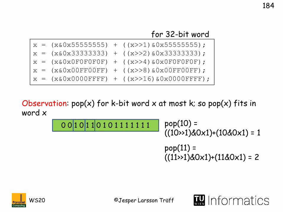
184
x = (x&0x55555555) + ((x>>1)&0x55555555);
x = (x&0x33333333) + ((x>>2)&0x33333333);
x = (x&0x0F0F0F0F) + ((x>>4)&0x0F0F0F0F);
x = (x&0x00FF00FF) + ((x>>8)&0x00FF00FF);
x = (x&0x0000FFFF) + ((x>>16)&0x0000FFFF);
Observation: pop(x) for k-bit word x at most k; so pop(x) fits in word x
0 0 1 0 1 1 0 1 0 1 1 1 1 1 1 1 pop(10) = ((10>>1)&0x1)+(10&0x1) = 1
pop(11) =((11>>1)&0x1)+(11&0x1) = 2
for 32-bit word

©Jesper Larsson TräffWS20
185
x = ~(~x&(x+1));
x = x-((x>>1)&0x55555555);
x = (x&0x33333333) + ((x>>2)&0x33333333);
x = (x+(x>>4)) & 0x0F0F0F0F;
x += (x>>8);
x += (x>>16);
z = x&0x0000003F;
0 0 1 0 1 1 0 1 0 1 1 1 1 1 1 1
Method 4a: implement popcount, improved
Here: 16-bit word
for 32-bit word
Exercise: Figure out what this does and why it works

©Jesper Larsson TräffWS20
186
Preprocessing for FFT: Bit reversal
Bit-reversal permutation often needed, e.g., efficient Fast Fourier Transform (FFT):B[r(i)] = A[i], where r(i) is the number arising from reversing the bits in the binary representation of i
Examples:
r(111000) = 000111r(10111) = 11101r(101101) = 101101
General: r(ab) = r(b)r(a)

©Jesper Larsson TräffWS20
187
x = ((x&0x55555555)<<1) | ((x&0xAAAAAAAA)>>1);
x = ((x&0x33333333)<<2) | ((x&0xCCCCCCCC)>>2);
x = ((x&0x0F0F0F0F)<<4) | ((x&0xF0F0F0F0)>>4);
x = ((x&0x00FF00FF)<<8) | ((x&0xFF00FF00)>>8);
x = ((x&0x0000FFFF)<<16) | ((x&0xFFFF0000)>>16);
for 32-bit word
r(a) for 32-bit word: Recursively, in parallel; branch-free:
0 0 1 0 1 1 0 1 0 1 1 1 1 1 1 1
0 0 0 1 1 1 1 0 0 1 1 1 1 1 1 1
1 0 1 1 0 1 0 0 1 1 1 1 1 1 1 0
0 1 0 0 1 0 1 1 1 1 1 0 1 1 1 1
1 1 1 1 1 1 1 0 1 0 1 1 0 1 0 0
Note: the assignments can be done in any order
©Jesper Larsson TräffWS20
188
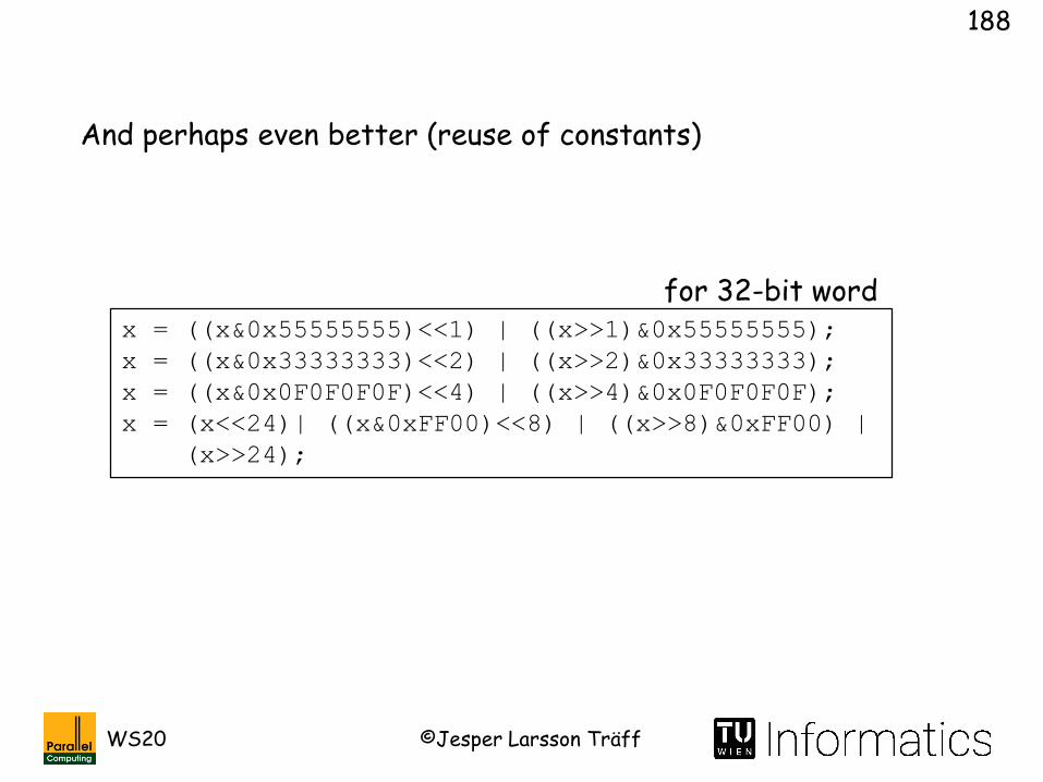
x = ((x&0x55555555)<<1) | ((x>>1)&0x55555555);
x = ((x&0x33333333)<<2) | ((x>>2)&0x33333333);
x = ((x&0x0F0F0F0F)<<4) | ((x>>4)&0x0F0F0F0F);
x = (x<<24)| ((x&0xFF00)<<8) | ((x>>8)&0xFF00) |
(x>>24);
for 32-bit word
And perhaps even better (reuse of constants)

©Jesper Larsson TräffWS20
189
Finding largest/smallest power of 2
int ispoweroftwo(long x) {
return (((x-1)&x)==0);
}
Detect whether x is a power-of-two; find smallest y=2k with y≥x
Find smallest: lsb(r(x)).
x = x-1;
x = x | (x>>1);
x = x | (x>>2);
x = x | (x>>4);
x = x | (x>>8);
x = x | (x>>16); x++;
for 32-bit word
Better, direct method:
Exercise: Find largest k s.t.2k≤x (aka msb(x), see lsb(x))

©Jesper Larsson TräffWS20
191
“If you write optimizing compilers or high-performance code, you must read this book”,Guy L. Steele, Foreword to “Hackers Delight”, 2002
D. E. Knuth: “The Art of Computer Programming”, Vol . 4A, Section 7.1.3, Addison-Wesley, 2011D. E. Knuth: “MMIXWare: A RISC Computer for the Third Millenium”, LNCS 1750, 1999 (new edition 2014)
See alsohttp://graphics.stanford.edu/~seander/bithacks.html
Are such things relevant?
Roofline model: Bitwise techniques/word parallelism can increase OI (operational intensity)
©Jesper Larsson TräffWS20
192
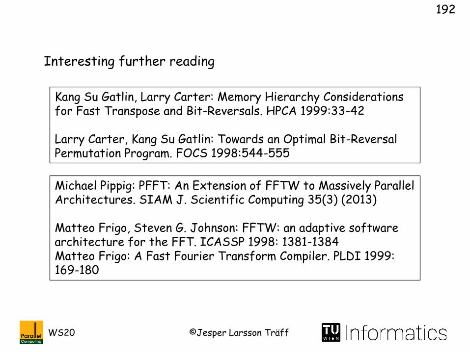
Michael Pippig: PFFT: An Extension of FFTW to Massively Parallel Architectures. SIAM J. Scientific Computing 35(3) (2013)
Matteo Frigo, Steven G. Johnson: FFTW: an adaptive software architecture for the FFT. ICASSP 1998: 1381-1384Matteo Frigo: A Fast Fourier Transform Compiler. PLDI 1999: 169-180
Kang Su Gatlin, Larry Carter: Memory Hierarchy Considerations for Fast Transpose and Bit-Reversals. HPCA 1999:33-42
Larry Carter, Kang Su Gatlin: Towards an Optimal Bit-Reversal Permutation Program. FOCS 1998:544-555
Interesting further reading

©Jesper Larsson TräffWS20
193
Not the end of the story
MPI_Comm_split(oldcomm,color,key,&newcomm);
All processes (in oldcomm) that supply the same color (or MPI_UNDEFINED) will belong to same newcomm, ordered by key, tie-break by rank in oldcomm
Problem: rank i supplying color c needs to determine which other processes also supplied color c
Trivial solution: all processes gather all colors and keys (MPI_Allgather), sort lexicographically to determine rank in newcomm
Early mpich (mid-90ties): bubblesort!!!
©Jesper Larsson TräffWS20
194
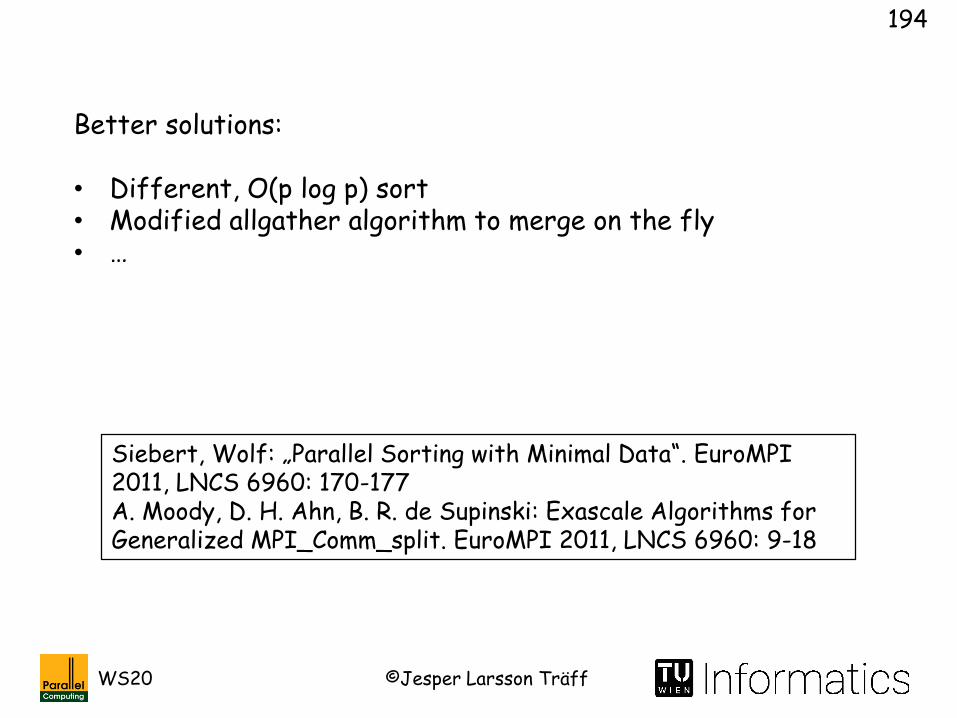
Siebert, Wolf: „Parallel Sorting with Minimal Data“. EuroMPI2011, LNCS 6960: 170-177A. Moody, D. H. Ahn, B. R. de Supinski: Exascale Algorithms forGeneralized MPI_Comm_split. EuroMPI 2011, LNCS 6960: 9-18
Better solutions:
• Different, O(p log p) sort• Modified allgather algorithm to merge on the fly• …