high performance data mining techniques for intrusion
TRANSCRIPT
University of Central Florida University of Central Florida
STARS STARS
Electronic Theses and Dissertations, 2004-2019
2004
High Performance Data Mining Techniques For Intrusion High Performance Data Mining Techniques For Intrusion
Detection Detection
Muazzam Ahmed Siddiqui University of Central Florida
Part of the Computer Sciences Commons, and the Engineering Commons
Find similar works at: https://stars.library.ucf.edu/etd
University of Central Florida Libraries http://library.ucf.edu
This Masters Thesis (Open Access) is brought to you for free and open access by STARS. It has been accepted for
inclusion in Electronic Theses and Dissertations, 2004-2019 by an authorized administrator of STARS. For more
information, please contact [email protected].
STARS Citation STARS Citation Siddiqui, Muazzam Ahmed, "High Performance Data Mining Techniques For Intrusion Detection" (2004). Electronic Theses and Dissertations, 2004-2019. 117. https://stars.library.ucf.edu/etd/117
HIGH PERFORMANCE DATA MINING TECHNIQUES FOR INTRUSION DETECTION
by
MUAZZAM SIDDIQUI B.E. NED University of Engineering & Technology, 2000
A thesis submitted in partial fulfillment of the requirements for the degree of Master of Science in the School of Computer Science
in the College of Engineering & Computer Science at the University of Central Florida
Orlando, Florida
Spring Term 2004
Major Professor: Joohan Lee

ABSTRACT
The rapid growth of computers transformed the way in which information and data was
stored. With this new paradigm of data access, comes the threat of this information being
exposed to unauthorized and unintended users. Many systems have been developed which
scrutinize the data for a deviation from the normal behavior of a user or system, or search for a
known signature within the data. These systems are termed as Intrusion Detection Systems
(IDS). These systems employ different techniques varying from statistical methods to machine
learning algorithms.
Intrusion detection systems use audit data generated by operating systems, application
softwares or network devices. These sources produce huge amount of datasets with tens of
millions of records in them. To analyze this data, data mining is used which is a process to dig
useful patterns from a large bulk of information. A major obstacle in the process is that the
traditional data mining and learning algorithms are overwhelmed by the bulk volume and
complexity of available data. This makes these algorithms impractical for time critical tasks like
intrusion detection because of the large execution time.
Our approach towards this issue makes use of high performance data mining techniques
to expedite the process by exploiting the parallelism in the existing data mining algorithms and
the underlying hardware. We will show that how high performance and parallel computing can
be used to scale the data mining algorithms to handle large datasets, allowing the data mining
component to search a much larger set of patterns and models than traditional computational
platforms and algorithms would allow.

We develop parallel data mining algorithms by parallelizing existing machine learning
techniques using cluster computing. These algorithms include parallel backpropagation and
parallel fuzzy ARTMAP neural networks. We evaluate the performances of the developed
models in terms of speedup over traditional algorithms, prediction rate and false alarm rate. Our
results showed that the traditional backpropagation and fuzzy ARTMAP algorithms can benefit
from high performance computing techniques which make them well suited for time critical
tasks like intrusion detection.

TABLE OF CONTENTS
LIST OF FIGURES ........................................................................................................... vi
LIST OF TABLES............................................................................................................ vii
CHAPTER 1: INTRODUCTION....................................................................................... 1
CHAPTER 2: RELATED RESEARCH ............................................................................. 3
Intrusion Detection ......................................................................................................... 3 Intrusion ..................................................................................................................................3 Intrusion Detection..................................................................................................................3 Intrusion Detection System .....................................................................................................4 Classification of intrusion detection........................................................................................5
Architecture...................................................................................................................................... 6 Information Source........................................................................................................................... 6 Analysis Type................................................................................................................................... 8 Timing .............................................................................................................................................. 9
A survey of intrusion detection research...............................................................................10
Data Mining .................................................................................................................. 14 A survey of intrusion detection research using data mining .................................................17
Neural Networks ........................................................................................................... 18 Neural Network Architectures ..............................................................................................21
Single Layer Feed Forward Networks............................................................................................ 21 Multi Layer Feed Forward Networks ............................................................................................. 23 Fuzzy ARTMAP Neural Networks ................................................................................................ 24
Learning Procedures..............................................................................................................26 Learning Algorithms .............................................................................................................28
Backpropagation Algorithm........................................................................................................... 29 Fuzzy ARTMAP Algorithm........................................................................................................... 31
Intrusion Detection using Neural Networks..........................................................................35 Neural Network Intruder Detector (NNID) .................................................................................... 36 Application of Neural Networks to UNIX Security ....................................................................... 36 Hierarchical Anomaly Network IDS using NN Classification....................................................... 37 Artificial Neural Networks for Misuse Detection .......................................................................... 38 Anomaly and Misuse Detection using Neural Networks................................................................ 38 UNIX Host based User Anomaly Detection using SOM ............................................................... 38 Host Based Intrusion Detection using SOM................................................................................... 39 Elman Networks for Anomaly Detection ....................................................................................... 40
CHAPTER 3: OUR APPROACH .................................................................................... 41
High Performance Data Mining.................................................................................... 42

High performance computing approach ................................................................................42 Motivation behind the work ..................................................................................................43 High performance approach for intrusion detection..............................................................44
Parallel Neural Networks.............................................................................................. 46 Large training time ................................................................................................................47 Approaches to improve efficiency ........................................................................................47 Parallel implementation of neural networks..........................................................................47 Our implementation environment .........................................................................................48 Neural networks architectures used.......................................................................................49 Parallel Backpropagation ......................................................................................................50 Parallelism in the BP Algorithm ...........................................................................................50
Network based Parallelism............................................................................................................. 51 Training Set Parallelism ................................................................................................................. 52
Parallel Backpropagation ......................................................................................................53 Algorithm ....................................................................................................................................... 53
Parallel Fuzzy ARTMAP ......................................................................................................58 Algorithm ....................................................................................................................................... 59
CHAPTER 4: EXPERIMENTAL RESULTS .................................................................. 65
Data preprocessing........................................................................................................ 68
Experiments .................................................................................................................. 69 Experiments with backpropagation .......................................................................................69 Experiments with fuzzy ARTMAP .......................................................................................73
CHAPTER 5: CONCLUSIONS ....................................................................................... 79
LIST OF REFERENCES.................................................................................................. 80
LIST OF FIGURES
Figure 1: A generic intrusion detection system. ............................................................................. 5 Figure 2: Data mining ................................................................................................................... 15 Figure 3: A 4 input, 3 hidden and 2 output nodes neural network................................................ 19 Figure 4: Model of a neuron ......................................................................................................... 20 Figure 5: Single layer feed forward neural network ..................................................................... 22 Figure 6: Multi layer feed forward network ................................................................................. 23 Figure 7: A block diagram of the fuzzy ARTMAP architecture. ................................................. 25 Figure 8: Illustration of supervised learning................................................................................. 27 Figure 9: Illustration of unsupervised learning. The cross marks (designated by the letter X)
indicate that the corresponding blocks are not available. ..................................................... 28 Figure 10: Network partitioning using vertical slicing scheme. ................................................... 52 Figure 11: Training set partitioning of English alphabets. ........................................................... 53 Figure 12: Execution times for backpropagation for a single epoch in logarithmic scale for full
dataset. .................................................................................................................................. 70 Figure 13: Execution times for backpropagation for a single epoch in logarithmic scale for 10%
dataset ................................................................................................................................... 72 Figure 14: Training times for fuzzy ARTMAP for a single epoch in logarithmic scale for full
dataset ................................................................................................................................... 75 Figure 15: Training times for fuzzy ARTMAP for a single epoch in logarithmic scale for 10%
dataset ................................................................................................................................... 77

LIST OF TABLES
Table 1: Attack types in the training data set................................................................................ 66 Table 2: Basic features of individual TCP connections................................................................ 67 Table 3: Content features within a connection suggested by domain knowledge ........................ 67 Table 4: Features computed using a two-second time window. ................................................... 68 Table 5: Training times for a single epoch for parallel backpropagation for full dataset............. 70 Table 6: Setup times for parallel backpropagation for full dataset ............................................... 71 Table 7: Training times for a single epoch for parallel backpropagation for 10% dataset ........... 72 Table 8: Setup times for parallel backpropagation for 10% dataset ............................................. 73 Table 9: Performance of parallel backpropagation algorithm. ..................................................... 73 Table 10: Training times for a single epoch on parallel fuzzy ARTMAP for full dataset ........... 74 Table 11: Setup times for fuzzy ARTMAP for full dataset. ......................................................... 76 Table 12: Training times for a single epoch on parallel fuzzy ARTMAP for 10% dataset.......... 77 Table 13: Distribution times on parallel fuzzy ARTMAP for 10% dataset................................. 78 Table 14: Performance of parallel fuzzy ARTMAP algorithm .................................................... 78

CHAPTER 1: INTRODUCTION
Computers have become an essential component of our daily lives. The World Wide Web
has transformed the world into a global village. Everyday there are millions of transactions on
the Internet. A tremendous amount of information and data is shared by the World Wide Web
users all over the world. The problem of protecting this information and data has become more
important, as the size of this network of interconnected machines is increasing dramatically
everyday. The number of security incidents reported in 2002 by CERT is 833% more than in
1999 [1]. The number of incidents in the first three quarters of 2003 outnumbered the previous
year figure.
Many methods have been developed to secure the infrastructure and communication over
the Internet. These techniques include firewalls, data encryption and virtual private networks.
Intrusion detection is relatively newer addition to this family of cyber guards. Intrusion detection
systems first appeared in early 1980s but they were limited for mostly military purposes.
Although commercial products became available in late 1980s, it was not until mid and late
1990s that intrusion detection systems started enjoying popularity with the explosion of the
Internet [5].
Intrusion detection systems are the systems designed to monitor computer and network
activities for security violations. These activities are observed by scrutinizing the audit data
generated by the operating system or some other application programs running on the computer.
With the availability of microprocessors that perform billions of operations in a second and high
speed network connections, the size of the file recording all these events usually reach in the

order of gigabytes. Dealing with such a huge amount of data is not a trivial task and specialized
methods are needed to process its information contents. To unearth useful patterns of previously
unknown information from a data source is a process, termed as data mining. Data mining is an
information extraction activity whose goal is to discover hidden facts contained in a database.
Mining the large volumes of intrusion detection audit data requires a lot of computational
time and resources. Traditional data mining algorithms are overwhelmed by the sheer complexity
and bulkiness of the available data. They have become computationally expensive and their
execution times largely depend on the size of the data they are dealing with.
In this research we are presenting a high performance data mining approach to deal with
the high volumes of intrusion detection data. Our work makes use of high performance
distributed computing techniques to scale the existing data mining algorithms, making them
practical to use in time critical applications like intrusion detection. We used machine learning
algorithms to extract normal behavior patterns and attacks from network traffic data. Among the
various learning approaches, we chose backpropagation and fuzzy ARTMAP neural networks.
Neural networks are well suited for intrusion detection because of their prediction and
generalization capabilities, which makes them able to identify known and unknown intrusions.
We developed parallel versions of backpropagation and fuzzy ARTMAP algorithms that allowed
them to search a much larger set of patterns and models than traditional algorithms would allow.
We evaluated their performances in terms of speedup over sequential algorithms and negative
and false positive rates. The speedup gave the measure of the high performance part while
negative and false positive rates represent the classification efficiency of the algorithms.

CHAPTER 2: RELATED RESEARCH
Intrusion Detection
The word intrusion as defined in the Webster’s dictionary means
1. The act of intruding or the condition of being intruded on.
2. An inappropriate or unwelcome addition.
3. Law. Illegal entry upon or appropriation of the property of another.
Where intrude means
To put or force in inappropriately, especially without invitation, fitness, or permission
Intrusion
Based upon the above definitions, intrusion in the terms of information can be defined as
when a user of information tries to access such information for which he/she is not authorized,
the person is called intruder and the process is called intrusion.
Intrusion Detection
Intrusion detection is the process of determining an intrusion into a system by the
observation of the information available about the state of the system and monitoring the user
activities. Detection of break-ins or attempts by intruders to gain unauthorized access of the
system is intrusion detection.

The intruders may be an entity from outside or may be an inside user of the system trying
to access unauthorized information. Based upon this observation intruders can be widely divided
into two categories; external intruders and internal intruders. [2]
• External intruders are those who don’t have an authorized access to the system
they are dealing with.
• Internal intruders are those who have limited authorized access to the systems
and they overstep their legitimate access rights.
Internal users can be further divided into two categories; masqueraders and clandestine
users.
• Masqueraders are those who use the identification and authorization of other
legitimate users.
• Clandestine users are those who successfully evade audit and monitoring
measures.
Intrusion Detection System
An intrusion detection system or IDS is any hardware, software or combination of both
that monitors a system or network of systems for a security violation [3].An IDS is often
compared with a burglar alarm system. Just like a burglar alarm system monitors for any
intrusion or malicious activity in a building facility, IDS keeps an eye on intruders in a computer
or network of computers [4].

Figure 1 displays a generic intrusion detection system. From the audit data source the
information goes to the pattern matching module for misuse detection and a profile engine to
compare current profile with the normal behavior defined for the system. Pattern matching
module interacts with policy rules to look for any signature defined in the policy. An anomaly
detector distinguishes an abnormal behavior using the profile engine.
Audit Data Source
Pattern Matcher
Profile Engine
Anomaly Detector
Policy Rules
Alarm/Report Generator
Figure 1: A generic intrusion detection system.
Classification of intrusion detection
There are many strategies to detect intrusions. Some of them involve monitoring user
activities while some involve examining system logs or network traffic for some specific
patterns. There are some attributes that classify these strategies for intrusion detection. These
attributes are architecture, information source, analysis type and timing [5].

Architecture
There are two types of intrusion detection systems according to the architecture. One
which are implemented on the system they are monitoring and others which are implemented
separately. This separate implementation has several advantages over the other approach.
• It keeps a successful intruder from disabling the intrusion detection system by
deleting or modifying the audit records on which the system is based.
• It lessens the load associated with running the intrusion detection system on the
monitored system.
The only disadvantage with this scheme is that it requires secure communication between
the monitoring and monitored system.
Information Source
The first and foremost source for intrusion detection is the data source. Data can be
obtained from system logs or packet sniffers or some other source. Depending upon the origin of
data source, intrusion detection can be classified into four categories; host based, network based,
application based and target based systems.
Host based intrusion detection involves the data that is obtained from sources internal to
a system. These include the operating system audit trails and system logs.The operating system
audit trails is a record of system events generated by the operating system. These system events
results from user actions and the process invoked on behalf of the user, whenever either makes a
system call or execute a command. A system log is a file of system events and settings. It is

different from audit trails in the sense that it is generated by a log-generation software within the
operating system and it is stored as a file.
Network based intrusion detection uses the data collected from the network traffic stream.
It is the most common information source in the intrusion detection systems because of the three
reasons. First, it can be accomplished by placing the network interface card in promiscuous mode
which has a very low or even no affect on the performance on the system being monitored.
Second, it can be transparent to the users on the network. And the third, there are some very
common types of attacks that are not easily detected by the host based systems. These include
various denial of service attacks.
Application based intrusion detection uses the data obtained from application softwares
such as web servers or some security devices. Many firewalls, access control systems and other
security devices generate their own event logs which contain information of security
significance.
Target based intrusion detection doesn’t require event data from any internal or external
source. Instead this scheme provides means of determining if the existing data in the system has
been modified in some fashion. Target based monitors use cryptographic hash functions to detect
alterations to the system objects and then compare these alterations to some defined policy to
detect any intrusion.

Analysis Type
Once the data is obtained, the next step is to analyze the data. There are two broad
categories into which intrusion detection can be classified according to the analysis performed;
anomaly detection and misuse detection.
Anomaly detection looks for any abnormal or unusual patterns in the data. It involves
defining and characterizing a normal behavior of the system in the static form or dynamic and
then flagging any event that deviates from the defined behavior. Since anomaly detection looks
for unusual pattern, therefore any unseen pattern that was not defined in the base profile of the
system will flag an intrusion. For this reason anomaly detection will suffer false positives.
(Normal behavior detected as abnormal) To combat this certain techniques are devised. Instead
of using a yes/no approach, intrusion detection systems use some statistical measures to figure
out the degree of anomalousness and a threshold value then gives the final decision. Anomaly
detection can be divided into two classes; static anomaly detection and dynamic anomaly
detection.
Static anomaly detection checks for data integrity in the system. A system normal state is
defined which represents the system code and a portion of the system data that should remain
constant. This state is then compared with any other state defined later to check for any alteration
which flags an intrusion if found positive.
Dynamic anomaly detection creates a base profile of the system’s normal behavior and
checks it against any new profile created. For each feature selected to define the base profile, a
list of observed values is recorded and inserted into the profile. Any new profile that
characterizes the system observed behavior is compared against the base profile.

Misuse detection is also called signature detection as it looks for specific signature
patterns in the data. Misuse detection searches for known intrusions in the data regardless of the
system normal behavior. The signature patterns misuse detection is looking for can be a static bit
string e.g. a virus or it can be a set of events or actions a user might take. In either case, the
searched patterns are already defined to be bad. Since misuse detection looks for only known
intrusions, it suffers from false negatives (Attacks identified as normal patterns), if the pattern in
question was not defined to be bad previously.
Timing
Based upon the timing intrusion detection can be classified roughly into two categories;
real time intrusion detection and interval/batch intrusion detection.
Real time intrusion detection means that the information source is analyzed in real-time.
This is the most desirable form of intrusion detection because the ultimate goal of intrusion
detection is to prevent an attack before it happens. But there are certain types of attacks which
can only be detected by observing the data for a certain period of time. Most commercial systems
employing real-time intrusion detection actually define a window size of 5 to 15 minutes.
Batch mode analysis means that the information source is analyzed in a batch fashion.
Data for a large interval of time, e.g. a day, is monitored at the end of the interval (in this case,
end of the day).

A survey of intrusion detection research
As described earlier, an intrusion detection system is a system that tries to detect break-
ins or break-in attempts into a computer system or network by monitoring network packets,
system files or log files. This section describes a survey of research in the intrusion detection
systems. The survey classifies all the systems covered according to the classification criteria
described in the previous section. In addition it also describes the basic approach taken by each
system to detect intrusions. These include rule based systems, statistical analysis, neural
networks and data mining approaches. All the systems described here focuses on the
classification accuracy and none of them address the issue of learning time though some [50, 51]
report large volumes of data to be a factor hindering in research.
EMERALD – Event Monitoring Enabling Responses to Anomalous Live Disturbances
EMERALD [41] is a real-time hybrid analysis type intrusion detection system employing
both anomaly and misuse detection. It is intended to be a framework for scalable, distributed,
interoperable computer and network intrusion detection. It uses a three layer approach to large
scale intrusion detection. Each of these layers has monitors. The lowest layer called service layer
monitors a single domain. The middle layer called domain-wide accepts inputs from the lowest
layer and detects intrusion across multiple single domains. Similarly the topmost layer called
enterprise-wide accepts inputs from middle layer and detects intrusion across the entire system.

IDES – Intrusion Detection Expert System
IDES [42] is a real-time host based anomaly detection system. It is considered to be the
pioneer in the anomaly detection approach. The basic motivation behind IDES approach was that
the users behave in a consistent manner from time to time, when performing their activities on
the computer. The manner in which they behave can be summarized by calculating various
statistics for their behavior. IDES applied a rule based approach to determine user’s behavior.
NIDES – Next Generation Intrusion Detection System
NIDES [43] is an extension to IDES which was a rule based anomaly detection system.
NIDES is a real-time host based system with a misuse detection component in addition to the
anomaly detection engine. The rule based component was based upon Product-Based Expert
System Toolset (P-BEST) which is a forward-chaining LISP based environment. Four major
versions were released for NIDES each with refinements as a result of further research and users
inputs. In these versions the misuse detection part used the older rule based approach while the
anomaly detection functionality was changed to statistical based analysis. NIDES builds
statistical profile of users, though the entities monitored can also be workstations, network of
workstations, remote hosts, groups of users, or application programs. A statistical unusual
behavior from the user flags an intrusion into the system.
MIDAS – (Multics Intrusion Detection and Alerting System)
MIDAS [44] is a real-time host based system employing both anomaly and misuse
detection. The basic concept behind MIDAS was heuristic intrusion detection. MIDAS rules

were divided into two parts; primary rules and secondary rules. Primary rules describe some pre-
defined action when an intrusion is detected while secondary rules determine the type of action
that should be taken by the system. MIDAS is considered to be the first system employing
misuse detection.
Tripwire
Tripwire [45] is a static anomaly detector that uses a target based information source. It is
a file integrity checker that uses signatures as well as Unix file meta-data. It calculates
cryptographic checksum of critical files. The information is stored in a file called tw.config.
Periodically, Tripwire re-calculates the checksum. Any change to a file results in a checksum
change which indicates an abnormal activity.
CSM – Cooperative Security Manager
CSM [46] is a real-time, host based, distributed intrusion detection system. Each
computer on the network runs a copy of the security manager. This manager is responsible of
detecting anomaly and misuse detection on the local system as well as intrusive behavior
originating from the original user of the machine. When a user accesses a host from another host,
the managers exchange information about the user and the connection. The site security officer
can trace a connection request. An alarm is raised if the same user is trying to connect from two
different locations.

GrIDS – Graph based Intrusion Detection System
GrIDS [47] is a graph based intrusion detection system for large networks. It operates in
batch mode on both host and network traffic data. The graph based approach considers host as
nodes and the connections between hosts and edges on a graph. It uses a decentralized approach
and the system being observed is broken down into hierarchical domains. Each domain
constructs its own graph and sends its analysis to its parent domain. A rule set is used to build
graphs from incoming and previous information. A possible intrusion is determined again by a
set of rules.
NSM – Network Security Monitor
NSM [48] is a real-time network based intrusion detection system with a strong tendency
towards misuse detection. It was the first system to use raw network traffic as information
source. As a result NSM can monitor for a network of heterogeneous hosts without having to
convert the data into some canonical form. Since NSM is implemented on a separate system it
doesn’t consume resources from the monitored host.
NNID – Neural Network Intruder Detector
NNID [49] is a batch-mode host based anomaly detection system. It defines a normal
behavior of a user by using the distribution of commands he/she executes. This system uses a
backpropagation neural network for user behavior analysis. At fixed intervals, the collected data
is used to train the network. Once trained, the system monitors for user activities and detect any
anomalous behavior.

MADAM ID – Mining Audit Data for Automated Models for Intrusion Detection
MADAM ID [50] is a network based intrusion detection system that uses a data mining
approach to detect anomaly as well as misuse detection. The main components of MADAM ID
are classification and meta-classification programs, association rules and frequent episodes
programs, a feature construction system, and a conversion system that translates off-line learned
rules into real-time modules.
ADAM – Audit Data Analysis and Mining
ADAM [51] is a real-time network based anomaly detection system. It employs data
mining to extract association rules from the audit data. ADAM works by creating a customizable
profile of rules of normal behavior and it contains a classifier that distinguishes the suspicious
activities, classifying them into real attacks and false alarms.
Data Mining
Data mining, also known as Knowledge Discovery in Databases (KDD) has been
recognized as a rapidly emerging research area. This research area can be defined as efficiently
discovering human knowledge and interesting rules from large databases. Data mining involves
the semiautomatic discovery of interesting knowledge, such as patterns, associations, changes,
anomalies and significant structures from large amounts of data stored in databases and other
information repositories [6].
Data mining is an information extraction activity whose goal is to discover hidden facts
contained in databases. Using a combination of machine learning, statistical analysis, modeling

techniques and database technology, data mining finds patterns and subtle relationships in data
and infers rules that allow the prediction of future results.
Artificial Intelligence Database Theory
Statistics
Data Warehousing
Machine Learning
Data Mining
Figure 2: Data mining
Figure 2 displays how database theory, statistics and artificial intelligence approaches are
used in data mining.
Data mining sorts through data to identify patterns and establish relationships. Data
mining parameters include: association, sequence analysis, classification, clustering, forecasting
• Association - looking for patterns where one event is connected to another event.
• Sequence or path analysis - looking for patterns where one event leads to another
later event.

• Classification - looking for new patterns (May result in a change in the way the
data is organized but that's ok).
• Clustering - finding and visually documenting groups of facts not previously
known.
• Forecasting - discovering patterns in data that can lead to reasonable predictions
about the future.
For every data mining system, a data preprocessing step is one of the most important
aspects. Data preprocessing consumes 80% time of a typical, real world data mining effort. Poor
quality of data may lead to nonsensical data mining results which will subsequently have to be
discarded. Data preprocessing concerns the selection, evaluation, cleaning, enrichment, and
transformation of the data. Data preprocessing involves the following aspects: [7]
Data cleaning is used to ensure that the data are of a high quality and contain no
duplicate values. The data-cleaning process involves the detection and possible elimination of
incorrect and missing values.
Data integration. When integrating data, historic data and data referring to day-to-day
operations are merged into a uniform format.
Data selection involves the collection and selection of appropriate data. The data are
collected to cover the widest range of the problem domain.
Data transformation involves transforming the original data set to the data
representations of the individual data mining tools.

A survey of intrusion detection research using data mining
Over the past few years a growing number of research projects have applied data mining
for intrusion detection. The research could date back to 1984 when the development of Wisdom
& Sense [52] started and then published in 1989. Wisdom & Sense was the first work to mine
association rules from audit data. But it was not until recently that researchers started realizing
that the data size they are dealing with is getting larger and larger and to analyze data manually is
not possible anymore for extracting patterns of information. Data mining was viewed as a
solution to this problem. Our work in this thesis is also driven by the same motivation.
This section presents a survey of research in applying data mining techniques for
intrusion detection.
W&S – Wisdom & Sense
Wisdom & Sense [52] (W&S) is a host based anomaly detection system. W&S studies
audit data to mine association rules that describes the normal behavior. This is called the
Wisdom part of W&S. The Sense part of W&S comprises of an expert system that analyze recent
audit data to monitor for any violation based upon the rules produced by the Wisdom part.
MADAM ID – Mining Audit Data for Automated Models for Intrusion Detection
MADAM ID [50] is considered to be one of the best data mining projects in intrusion
detection. It applies data mining programs to network audit data to compute misuse and anomaly
detection models, according to the observed behavior in the data. MADAM ID consists of
several components to construct concise and intuitive rules that can detect intrusions. MADAM

ID has a meta- learning component that constructs a combined model that incorporates evidence
from multiple models. A basic association rules and frequent episode algorithms component to
accommodate the special requirements in analyzing audit data. A feature construction system
and a conversion system that translates off-line learned rules into real-time modules.
ADAM – Audit Data Analysis and Mining
ADAM [51] is the second most widely known and published worked amongst the data
mining projects in intrusion detection. ADAM is a network anomaly detection system. The
ADAM approach includes detecting events and patterns explicitly defined by the system
operator, mining exclusively within a limited time window to detect recent “hot” associations,
comparing currently mined rules with a repository of aggregated past rules, testing rules with a
multi-algorithm classification engine, and applying post-processing filtering and prioritization of
alarms.
Neural Networks
Artificial Neural Networks, commonly known as “neural networks” have been an
academic disciple since the advent of the notion that brain computes in an entirely different
fashion from the conventional digital computer. The research was started over 50 years ago with
the publication by McCulloch and Pitts [8] of their famous result that any logical problem can be
solved by a suitable network composed of so-called binary decision nodes.
A neural network is a set of interconnected processing elements that has the ability to
learn through trial and error.
A neural network resembles the brain in two respects: [9]

• Knowledge is acquired by the network through a learning process.
• Connection strengths between the processing elements known as synaptic weights
are used to store the knowledge.
Figure 3 displays a feed forward neural network architecture with 4 input, 3 hidden and 2
output nodes.
Output nodes Hidden nodes Input nodes
Figure 3: A 4 input, 3 hidden and 2 output nodes neural network.
The processing elements in the neural network are called neurons. There are essentially
three basic elements of a neuron.
• A set of weighted connection links or synapses.
• An adder for summing the input signals, weighted by the respective synapses of
the neurons.
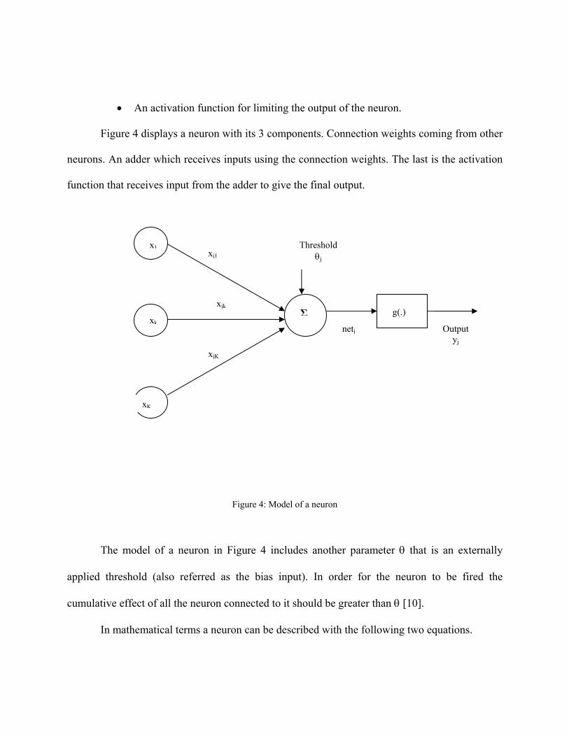
• An activation function for limiting the output of the neuron.
Figure 4 displays a neuron with its 3 components. Connection weights coming from other
neurons. An adder which receives inputs using the connection weights. The last is the activation
function that receives input from the adder to give the final output.
x1 Threshold xj1 θj
xjkΣ g(.)
xknetj Output
Figure 4: Model of a neuron
The model of a neuron in Figure 4 includes another parameter θ that is an externally
applied threshold (also referred as the bias input). In order for the neuron to be fired the
cumulative effect of all the neuron connected to it should be greater than θ [10].
In mathematical terms a neuron can be described with the following two equations.
xjK
yj
xK

netj = Σk=1K
wjkxk - θj
and
yj = g(netj)
where x1, x2, …, xk are the input signals, wj1, wj2, …, wjk are the synaptic weights
converging to neuron j, netj is the cumulative effect of all the neurons connected to neuron j and
the internal threshold of neuron j, g(.) is the activation function and yj is the output of the neuron.
Neural Network Architectures
The architecture of the neural network can be defined as the manner in which the neurons
and their interconnection links are arranged in the network. Neural networks need a learning
algorithm to train the neurons. The architecture of the network also depends upon the underlying
learning algorithm.
Keeping within the scope of our work we are only defining 3 neural network
architectures. First the simplest architecture found in the neural networks literature and the other
two are those that we used in our experiments.
Single Layer Feed Forward Networks
The neurons in a neural network are essentially arranged in the form of layers. The
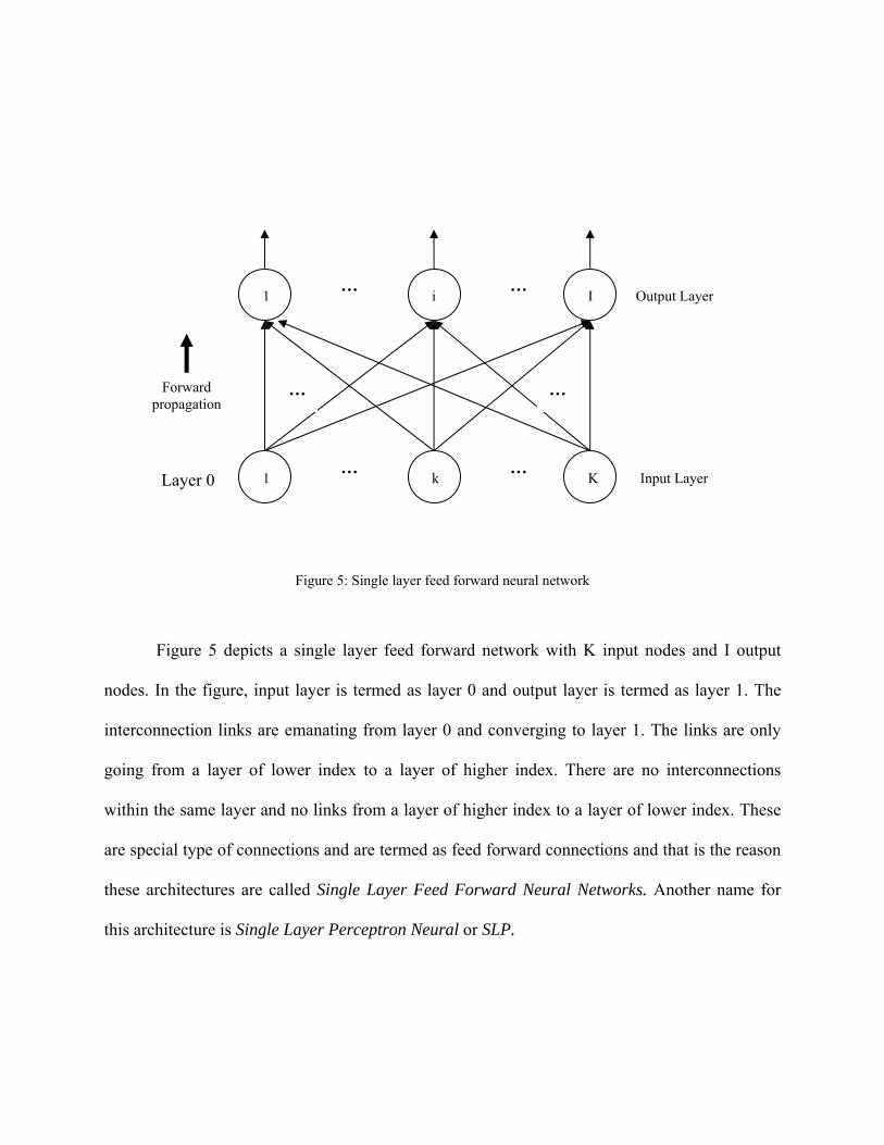
simplest possible arrangement is the single layer feed forward network that has one input layer
and one output layer. It is called single layer because only output layer has neurons. Input layer
nodes just register the input patterns applied to neural network.
… …
Figure 5: Single layer feed forward neural network
Figure 5 depicts a single layer feed forward network with K input nodes and I output
nodes. In the figure, input layer is termed as layer 0 and output layer is termed as layer 1. The
interconnection links are emanating from layer 0 and converging to layer 1. The links are only
going from a layer of lower index to a layer of higher index. There are no interconnections
within the same layer and no links from a layer of higher index to a layer of lower index. These
are special type of connections and are termed as feed forward connections and that is the reason
these architectures are called Single Layer Feed Forward Neural Networks. Another name for
this architecture is Single Layer Perceptron Neural or SLP.
… …
… …
Layer 0
Forward propagation
Input Layer
1 i I Output Layer
1 k K

Multi Layer Feed Forward Networks
The multi layer feed forward network is an extension to the single layer feed forward
network as it contains one or more layers in addition to the input and output layers. These layers
are called hidden layers and they are situated between input and output layers.
Figure 6: Multi layer feed forward network
…
… …
…
… …
… …
Layer 0
Layer 1
Forward propagation
Input Layer
Output Layer
1 k K
1 j J
1 i ILayer 2
1st Hidden Layer
Forward propagation
… …

Figure 6 depicts a multi layer feed forward network with one hidden layer. Input layer
with K nodes is designated as layer 0, hidden layer with J nodes is designated as layer 1 and
output layer with I nodes is designated as layer 2. As in single layer feed forward network
interconnections links are only from a layer of lower index to a layer of higher index. Signals are
propagated from input layer to hidden layer and then from hidden layer to output layer. This type
of connectivity is called standard connectivity and the connections are called feed forward
connections. That is the reason these architectures are called Multi Layer Feed Forward Neural
Networks or Multi Layer Perceptron (MLP).
Fuzzy ARTMAP Neural Networks
The third type of neural network architecture we are discussing is the fuzzy ARTMAP
which belongs to a special class of neural networks called Adaptive Resonance Theory (ART)
Neural Networks. [21]
Fuzzy ARTMAP neural network consists of two fuzzy ART modules designated as ARTa
and ARTb and as well as an interART module. Inputs are presented at the ARTa module while
ARTb module receives their corresponding outputs. The purpose of the interART module is to
establish a mapping between inputs and outputs.
Figure 7 displays a block diagram of the fuzzy ARTMAP system. The fuzzy ART
modules ARTa and ARTb are connected through an interART module Fab. An internal controller,
controls the creation of mapping between inputs and outputs patterns at Fab.

Fab
F2a F2
b
Top down weights
Top down weights
Internal Control F1
a F1b
ARTa ARTb
Figure 7: A block diagram of the fuzzy ARTMAP architecture.
Each of the ARTa and ARTb modules consists of three layers, input layer F0 (not shown
in the figure), choice layer F1 and matching layer F2.
The purpose of the input layers F0 in ARTa and ARTb modules is to preprocess the input
and output patterns presented to these modules respectively. The processing involved is called
complement coding and it converts an M dimensional vector a = (a1, …, aM) to 2M dimensional
vector I such that
I = (a, ac) = (a1, …, aM, a1
c, …, aMc)
Where,

aic = 1 – ai 1 ≤ i ≤ M
Choice layer F1a in ARTa contains 2Ma nodes where Ma is the input dimensionality.
Similarly F2b in ARTb has 2Mb nodes where Mb is the output dimensionality. Matching layer F2a
and F2b have Na and Nb nodes respectively. Nx corresponds to the number of commited nodes
plus one uncommitted node. Commited nodes are the nodes in ARTa and ARTb modules which
have established a mapping. Each node in F1 is connected via a bottom up weight to each node in
F2. Similarly each node in F2 is connected via top down weights to each node in F1. These top
down weights are called ARTa and ARTb templates for the ARTa and ARTb modules respectively.
The interART module has one layer Fab of Nb nodes and has weights converging to its every
node from the F2a layer in ARTa module.
Learning Procedures
There are essentially two types of learning procedures involved with the neural networks;
supervised learning and unsupervised learning. Sometimes a third type of learning is also
employed which is the hybrid of the above two types and is called hybrid learning.
• Supervised learning, as the name implies, is the form of learning which is
managed by an external teacher. The learning patterns are applied to the network
and the teacher steers the process by providing the network, the target response to
the input patterns.

Environment Teacher
Figure 8: Illustration of supervised learning
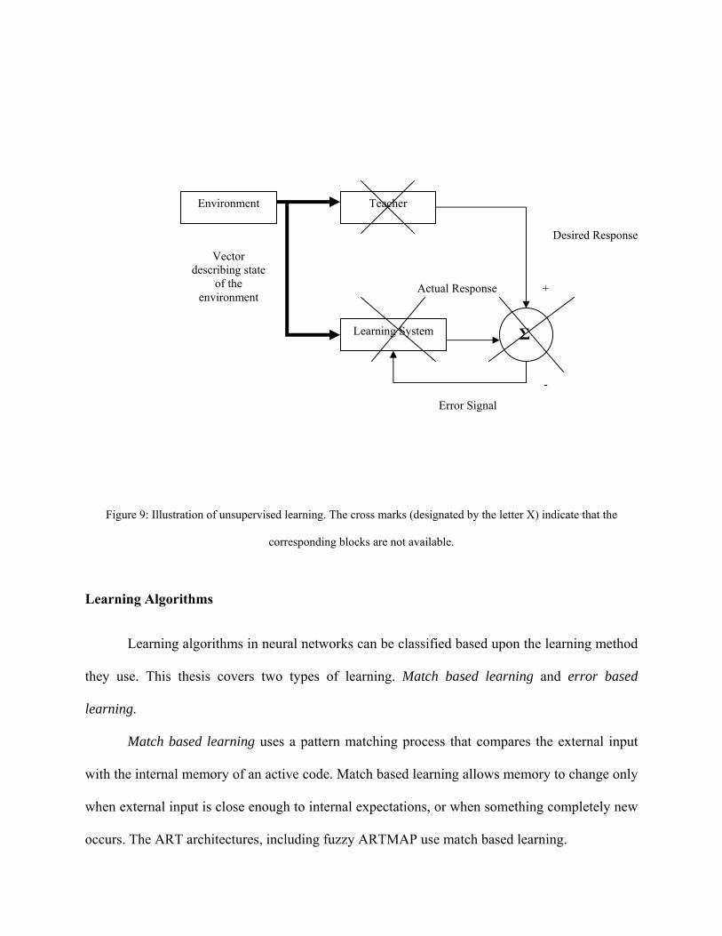
• Unsupervised learning doesn’t employ an external teacher for the learning
procedure. A desired response cannot be provided to the network, in the absence
of a teacher. Instead unsupervised learning uses another procedure called self-
organizing to learn the training patterns.
Learning System
Desired Response
Vector describing state
of the environment
Actual Response +
Σ
-
Error Signal
Environment Teacher
Figure 9: Illustration of unsupervised learning. The cross marks (designated by the letter X) indicate that the
corresponding blocks are not available.
Learning Algorithms
Learning algorithms in neural networks can be classified based upon the learning method
they use. This thesis covers two types of learning. Match based learning and error based
learning.
Match based learning uses a pattern matching process that compares the external input
with the internal memory of an active code. Match based learning allows memory to change only
when external input is close enough to internal expectations, or when something completely new
occurs. The ART architectures, including fuzzy ARTMAP use match based learning.
Learning System
Desired Response
Actual Response +
Σ
Vector describing state
of the environment
-
Error Signal

Error based learning responds to a mismatch by changing memories so as to reduce the
difference between a target output and the actual output, rather than by searching for a better
match. The difference between target output and actual output represents the error of the system
and error based learning tries to minimize this error. The famous backpropagation algorithm
employs error based learning.
Backpropagation Algorithm
Backpropagation algorithm is based on the error-correction learning rule under a
supervised learning environment. Backpropagation consists of two passes; a forward pass and a
backward pass. In the forward pass the inputs are applied to a multilayer perceptron and the
resulting signals are propagated forward layer by layer. Finally an actual response is produced as
the output of the network. The weights of the network remain unchanged in this pass. During the
backward pass, on the other hand, the synaptic weights are changed according to the error-
correction rule. Specifically, the actual response is subtracted from the desired response of the
network to produce an error signal. This error signal is then propagated backward through the
layers of the network, hence the name error backpropagation. The synaptic weights are adjusted
so as to make the actual response of the network move closer to the desired response.
The following notations are used in the description of the algorithm below.
PT total number of patterns
N total number of processors
K number of nodes in the input layer
J number of nodes in the hidden layer

I number of nodes in the output layer
xk(p) input for pattern p
yj2(p) calculated output for pattern p
di2(p) desired output for pattern p
yj1(p) hidden layer output for pattern p
wij2(t) current output layer weights
wjk1(t) current hidden layer weights
σi2(p) output layer error term for pattern p
σj1(p) hidden layer error term for pattern p
∆ wij2(t) current change in weight for output layer
∆ wjk1(t) current change in weight for hidden layer
∆ wij2(t-1) previous change in weight for output layer
∆ wjk1(t-1) previous change in weight for hidden layer
η learning rate
α momentum term
The backpropagation algorithm as a step by step procedure is presented as follows:
1. Initialize the weights in the MLP-NN architecture.
2. Present the input pattern x(p) to the input layer.
3. Calculate the outputs at the hidden and output layers.
yj1(p) = g(neti
1(p)) = g[Σk=0Kwjk
1(t).xk(p)] 1 ≤ j ≤ J
yj2(p) = g(neti
2(p)) = g[Σj=0Jwij
2(t).yj1(p)] 1 ≤ i ≤ I
4. Check to see if the actual output is equal to the desired output.

a. If yes, move to step 7.
b. If no, proceed with step 5.
5. Calculate the error terms associated with output and hidden layers.
σi2(p) = g’(neti
2(p))[di2(p) – yi
2(p)] 1 ≤ i ≤ I
σj1(p) = g’(netj
1(p)) Σi=1Iwij
2(t). σi2(p) 1 ≤ j ≤ J
6. Change the weights according to the error-correction rule.
∆ wij2(t) = η. σi
2(p). yj1(p) + α . ∆ wij
2 (t-1) 1 ≤ i ≤ I, 0 ≤ j ≤ J
∆ wjk1(t) = η. Σj
1(p). xk(p) + α . ∆ wjk1(t-1) 1 ≤ j ≤ J, 0 ≤ k ≤ K
7. Check to see if this pattern is the last in the set.
a. If no, go to step 2 and present the next pattern in the sequence.
b. If yes, check if the convergence criteria are satisfied.
i. If yes, the training is complete.
ii. If no, go to step 2 and present the first pattern from the training set.
Fuzzy ARTMAP Algorithm
Fuzzy ARTMAP uses incremental supervised learning of recognition categories and
multidimensional maps in response to an arbitrary sequence of analog or binary input patterns.
Fuzzy ARTMAP realizes a new minimax learning rule that cojointly minimizes the predictive
error and maximizes the code generalization. This is achieved by a match tracking process that
sacrifices the minimum amount of generalization necessary to correct a predictive error [11].
During the training, ARTa and ARTb modules receive a stream of input and output
patterns. The interART module receives inputs from both ARTa and ARTb modules. If a match is

found; i.e. the network’s prediction is confirmed by the selected target category, the network will
learn by modifying the prototype stored patterns of the selected ARTa and ARTb categories with
the new information. A mismatch results in a memory search leading to the selection of a new
ARTa category that better predicts the current ARTb category. The process continues till a better
prediction is found or a new ARTa category is created. In the later case, the network will learn by
storing a prototype pattern of the newly learned category.
The following notations are used in the description of the algorithm below.
ARTa ART Module for inputs
ARTb ART Module for outputs
F1a matching layer in ARTa
F1b matching layer in ARTb
F2a choice layer in ARTa
F2b choice layer in ARTb
Na number of nodes in F2a
Nb number of nodes in F2b
Ir input pattern r
Or output pattern r
^ fuzzy min operator performed on vectors and the result is the minimum of
the corresponding components
|x| size of the vector x which is equal to the sum of its components
Tja(Ir) bottom up input from node j in F1
a for pattern Ir
Tkb(Or) bottom up input from node j in F1
b for pattern Or

wja top down weight to node j in F1
a from F2a
wkb top down weight to node k in F1
b from F2b
βa ARTa choice parameter
βb ARTb choice parameter
jmax current winner node in ARTa
kmax current winner node in ARTb
wjmaxa top down weights corresponding to winner node jmax in ARTa
wkmaxb down weights corresponding to winner node kmax in ARTb
ρa vigilance parameter for ARTa
ρb vigilance parameter for ARTb
ε increment in the vigilance parameter
The fuzzy ARTMAP algorithm as a step by step procedure is presented as follows:
1. Initialize the weight vectors corresponding to the uncommitted nodes in F2a and F2
b to all-
ones.
2. Present the input/output pair to the network and set the vigilance to base-line vigilance.
3. Calculate the bottom up inputs to all the Na nodes in F2a.
Tja(Ir) = (| Ir ^ wj
a | ) / (βa + | wja |)
4. Choose the node in F2a that receives the maximum input from F1
a. Assume its index is
jmax. Check to see if it satisfies the vigilance criteria. We now distinguish three cases:
a. If node jmax is uncommitted node, it satisfies the vigilance criteria in ARTa. Go to
step 5.

b. If node jmax is commited node and it satisfies the vigilance criteria, go to step 5. A
node jmax satisfies the vigilance criteria if,
| Ir ^ wjmaxa | / | Ir | ≥ ρa
c. If node jmax does not satisfy the vigilance criteria, disqualify this node and go to
step 4.
5. Now consider three cases:
a. If node jmax is an uncommitted node, designate the mapping of jmax in F2a to kmax
in F2b. kmax is found by executing the following steps:
i. Calculate the bottom up inputs to all the Nb nodes in F2b.
Tkb(Or) = (| Or ^ wk
b | ) / (βb + | wkb |)
ii. Choose the node in F2b that receives the maximum input from F1
b. Assume
its index is kmax. Check to see if it satisfies the vigilance criteria. We now
distinguish three cases:
1. If kmax is an uncommitted node, it satisfies the vigilance criteria.
Increase Nb by one by introducing a new uncommitted node in F2b
and initialize its top down weights to all-ones. Go to step 5(a) ii-4.
2. If kmax is commited node and it satisfies the vigilance criteria, go to
step step 5(a)ii-4. A node kmax satisfies the vigilance criteria if.
| Or ^ wkmaxb | / | Or | ≥ ρb
3. If kmax is commited node and it does not satisfy the vigilance
criteria, disqualify this node by setting Tkmax(Or ) = -1 and go to
step 5(a) ii.

4. Now node jmax in F2a is mapped to node kmax in F2
b. The top-down
weights in ARTa and ARTb are updated.
wjmaxa = Ir ^ wjmax
a
wkmaxb = Or ^ wkmax
b
b. If node jmax is a commited node and due to prior learning this node is mapped to
node kmax and kmax satisfies the vigilance criteria, correct mapping is achieved and
weights in ARTa and ARTb are updated. If this is the last pattern in the training
set, go to step 6, otherwise go to step 2 and present the next in sequence pattern.
c. If node jmax is a commited node and due to prior learning this node is mapped to
kmax and kmax does not satisfy vigilance criteria, disqualify jmax by setting Tjmax(Ir )
= -1, increase the vigilance criteria in ARTa and go to step 4.
| Ir ^ wjmaxa | / | Ir | + ε
6. After all the patterns are presented, consider two cases:
a. If in the previous list presentation, at least one component of the top-down weight
vectors was changed, go to step 2 and present the first pattern in the training set.
b. If in the previous list presentation, no weight changed occurred, the training is
finished.
Intrusion Detection using Neural Networks
Neural networks have proven to be a promising modus operandi for intrusion detection.
A wide variety of intrusion detection systems are using neural networks to address the intrusion
detection problem. The primary reason for using the neural networks as the analysis engine in
IDS is their generalization ability which makes is suitable to detect unknown attacks.
The most common neural network architecture, used in the intrusion detection systems, is
the MLP architecture using a backpropagation algorithm or some variation of it. The earlier
works were mostly focused on anomaly detection on user behavior analysis. Later on, MLP were
used for misuse detection also as an alternative to other, rule-based, signature detection systems.
More recent work is focused on using unsupervised learning techniques to classify user behavior
analysis for anomaly detection. Among the most promising IDS architectures based upon neural
networks are those which use neural networks in conjunction with other detection engines to
improve efficiency and generalization.
The following is a list of several prominent research projects using neural networks for
intrusion detection, along with a brief description of each. [12].
Neural Network Intruder Detector (NNID)
This system uses an MLP for user behavior analysis [49]. The data on which it operates
represents a set of commands a user executes. At fixed intervals, the collected data was used to
train the network. Once trained, the system monitors for user activities and detect any anomalous
behavior. The reported false positive rate of the system was 7%, while the false negative rate was
4%.
Application of Neural Networks to UNIX Security
This project is one of the earliest systems to use neural networks for user anomaly
detection [53]. The system uses an MLP to attempt, in real time, to train and detect anomalies.

The system was designed is such a way that after a brief training session, it continuously modify
and adapt to the user behaviors in real time.
Anomaly Detection using Neural Networks
This project uses an MLP network to examine applications at process level to detect an
anomalous behavior [54]. The system uses the notion that regardless of user characteristics, an
anomalous behavior at the application level will generate activities at the process level that can
be deemed as anomalous. The false positive rate was 0% while the false negative rate was 20%.
Hierarchical Anomaly Network IDS using NN Classification
This system uses an MLP neural network in conjunction with a statistical analysis engine
[55]. In addition the system consists of modules organized in different layers, with a module in
lower layer reporting to the next one in higher layer.
The different modules in the system are:
• Probe to collect network traffic and abstract it into statistical variables.
• Event preprocessor collects data from probes and other agents and format it for
statistical analyzer.
• Statistical model compares the data to the reference model describing the
system’s normal behavior. A stimulus vector was created of the discrepancy and
forwarded to the neural network for further analysis.
• Neural network analyzes the stimulus vector for a normal or anomalous activity.

Artificial Neural Networks for Misuse Detection
This project was one of the first attempts to use neural networks for misuse detection
[56]. The system uses an MLP neural network to analyze network traffic data. Some
preprocessing was involved before the data is fed to the neural network. Certain fields of the
packets were selected, normalization was done and data fields were grouped and converted to
neural network readable format. In addition data was also marked as normal or attack.
Anomaly and Misuse Detection using Neural Networks
This system was the first that shifted focus in anomaly detection from user behavior
analysis to program behavior analysis [57]. In this system individual MLP networks were trained
on the normal behavior of the varying programs. The goal of the system was to generalize from
incomplete data and classify data as anomalous or normal.
At operation time, the system was monitored per session. During each session, several
programs were run with different input parameters. The processes resulting from these events
were fed to various neural networks and an anomaly grade was determined for each. A post
processing leaky bucket algorithms gather all the anomaly scores for all the events and a
threshold value decides for different combinations of accuracy levels.
UNIX Host based User Anomaly Detection using SOM
This system uses a self organizing map (SOM) for detection and analysis of user’s
activities over an extended period of time for an anomalous behavior [58]. It uses the assumption

that normal behavior is consistent and concentrated in a limited feature space. Conversely,
scattered and irregular behavior will signal an anomalous activity.
Features describing a user or an object were collected, normalized and reduced. An SOM
was trained on this data and the resulting network was assumed to be representing valid feature
space for legitimate use.
Host Based Intrusion Detection using SOM
This system uses a self organizing map (SOM) to examine session data by users in UNIX
bases environment to search for anomalous behavior [59]. The system collects the following
session data for analysis:
• User group
• Connection type
• Connection source
• Connection time
The analysis engine consists of two levels, a 3-map tier which summarizes the first three
input domains with respect to time, and the second aggregates and correlates the results of the
first level. The analysis engine groups the session with respect to the variables examined. Each
group can then be examined and associated with a particular user behavior – whether it is normal
or anomalous.

Elman Networks for Anomaly Detection
This system uses Elman network [61] to detect anomalous behavior [60]. Elman
networks are recurrent neural network with the ability to maintain a state of the system.
The Elman network works by predicting the next sequence given a present input and the
context. The actual next sequence is compared to the predicted sequence, and the difference
between them represents a measure of the anomaly.

CHAPTER 3: OUR APPROACH
In recent times, data is collected in various forms and methods. With the recent progress
in automated data gathering, the availability of cheap storage, database and emergence of web
technologies, the volume of data, many organizations and individual deal with, has increased
manifolds. There are millions of transactions taking place everyday and the same are being
stored into databases. Until recent past, this data was only used to archive information. However
it was realized that this information can be used in several other ways, besides being used as an
archive. A digging into this data can give interesting patterns and information which was
previously unknown. Since this data was initially stored in the databases, the process was called
Knowledge Discovery in Databases (KDD). Recent progress in information technology reveals
more sources for the data, especially the web. So the process is termed now simply as Data
Mining.
Mining these huge volumes of available data for hidden patterns is a tedious process that
requires a lot of computation time and resources. Traditional data mining and learning algorithms
are overwhelmed by the bulk volume and complexity of available data. They have become
computationally expensive with larger execution times, which often depend upon the volume of
the dataset in question. There are many time critical tasks which may not be able to stand these
large execution times. Intrusion detection is one such operation. The ultimate goal of an intrusion
detection system is to catch an intrusion when it is happening. Detecting an intrusion once it has
happened might not be adequate in certain cases. An unreasonably high execution time will

make a certain data mining algorithm, having an excellent prediction capability, unappealing for
practical purposes.
High Performance Data Mining
The information sources used for intrusion detection are mostly system audit logs and
network traffic data. These logs and traffic datasets consists of huge amount of information. The
system logs contain records of system events as generated by operating system or some
application software, while network traffic data contains network packet information. Data
mining provides a solution to extract useful information from this huge bank of knowledge. But
one of the major obstacles of using the traditional data mining algorithms towards intrusion
detection is that they are only able to deal with moderate amounts of data. Extracting patterns of
useful information for intrusion detection purposes from the huge audit files is not a trivial task.
The amount of audit data to be analyzed and its complexity is increasing dramatically. This
raises the issue of how to increase the computational capacity of data mining systems.
High performance computing approach
High performance data mining has arisen as an interdisciplinary response to this
situation, merging ideas and techniques drawn from disciplines such as statistics, pattern
recognition, machine learning, databases, and high performance computing. High performance
data mining tries to exploit the parallelism in the data mining algorithm and the underlying
hardware to cope with the increasing demand of lower execution times and higher volumes of
data. Current parallel processor and computing technologies can be used to make the data mining
process capable of dealing with massive databases in reasonable time. High performance

computing makes it possible to scale the existing data mining algorithm over various platforms.
Faster processing also means that users can experiment with more models to understand complex
data.
The approaches taken towards the scalable data mining algorithms include parallel
decision tree classifiers, parallel association rules, parallel instance-based learning, parallel
genetic algorithms and parallel neural networks [13].
Motivation behind the work
Previous and current research [14, 15, 16] shows that numerous approaches have been
taken to use different data mining algorithms for intrusion detection. However, not much
attention has been paid to the scalability and high performance issues of these algorithms. Most
of these algorithms are applied to a fraction of a large dataset. Larger execution times make it
infeasible to apply these algorithms to a dataset with millions of records in it.
We introduced a new strategy to address the issue of scalability of learning algorithms for
intrusion detection. The motivation behind the work was the fact that most of the research in the
area of intrusion detection is focused on classification accuracy and not much attention has been
paid to the learning times of the algorithms. As a result, smaller datasets with less than a million
records were used to perform the experiments which may not represent a real world scenario of a
log file containing more than 10 million or more records.
[26] presented a survey of various intrusion detection techniques including support vector
machines (SVMs), artificial neural networks (ANNs), multivariate adaptive regression splines
(MARS) and linear genetic programs (LGPs). The study used a dataset with less than 500,000

records and reported LGP to be the best classifier at the expense of time. Neural networks also
performed well but suffered the larger training times. Our approach solves the problem of large
training times. Faster learning also makes it possible to use real datasets in the experiments
instead of using a sample data.
High performance approach for intrusion detection
We used high performance data mining techniques to expedite the process by exploiting
the parallelism in the existing data mining algorithms and the underlying hardware. We showed
that how high performance parallel computing can be use to scale the data mining algorithms to
handle large datasets, allowing the data mining component to search a much larger set of patterns
and models than traditional computational platforms and algorithms would allow.
We used the anomaly detection approach for detecting intrusions in network traffic data.
Anomaly detection approach is based upon extraction of the normal behavior patterns out of a
huge datasets that we may not have any prior knowledge about. This extraction creates a model
of a normal system behavior and any deviation from it is considered as intrusion. Neural
networks are a natural choice for such an operation because of their generalization and prediction
capabilities. But neural networks suffer from the drawback of large training times. Considering
the amount of the data we have and the numbers of feature we need to define normal profiles
from the traffic data, traditional neural networks are not feasible option. We approached this
problem by employing parallelism in the classical neural networks learning algorithms. Among
the various available algorithms we chose backpropagation learning and fuzzy ARTMAP. Both

of these algorithms are well suited to identify patterns in the data and therefore are mainly used
for prediction and forecasting operations.
We implemented the parallel neural networks on a cluster computing environment.
Cluster computing is a process in which a set of computers connected by a network are used
collectively to solve a single large problem. Using a cluster of workstations has become a
popular method of solving both large and small scientific problems. The most important factor in
the success of cluster computing is cost. Massively parallel processors (MPP) cost more than $10
million while there is little cost involved in setting up a cluster of existing machines [32]. Early
supercomputers used distributed computing and parallel processing to link processors in a single
machine, often called a mainframe. Exploiting the same technology, cluster computing produces
computers with supercomputer performance for less than $40,000 [33]. Given this new
affordability, a number of universities and research laboratories are experimenting with installing
such systems in their facilities. These systems are termed as Beowulf clusters.
Beowulf is an approach to building a supercomputer as a cluster of commodity off-the-
shelf personal computers interconnected by widely available networking technology running any
one of several open-source Unix-like operating systems. Beowulf programs are usually written in
C or FORTRAN, adopting a message passing model of parallel computation but other open,
standards based approaches are possible, including process level parallelism, shared memory
(OpenMP, BSP), other languages (Java, LISP, FORTRAN90), and other communication
strategies (RPC, RMI, CORBA) [34].
The Beowulf idea is said to enable the average university computer science department or
small research company to build its own small supercomputer that can operate in the gigaflop

(billions of operations per second) range. Since Beowulf is mechanism of establishing a general
purpose loosely coupled parallel computing environment, it is not only cost effective but it also
decrease the dependency on particular hardware and software vendors. As off-the-shelf
technology evolves, a Beowulf can be upgraded to take advantage of it [34].
Our idea combines the potential of high performance approach with the cost effectiveness
and wide availability of cluster computing to scale the existing machine learning algorithms to
deal with much larger datasets in intrusion detection than traditional algorithms would allow.
High performance makes it practical for users to analyze greater quantities of data that, in turn,
yield improved predictions. We showed that how high performance computing can be used to
overcome performance limitations of the available hardware. The work will serve as a precursor
to the researchers in intrusion detection whose experiments are hindered by the high volumes of
data.
Parallel Neural Networks
Research in artificial neural networks was started almost 50 years ago with the famous
publication by McCulloch and Pitts [8]. Since then the eclectic nature of this field has inspired
researchers from such diverse disciplines as neuroscience, engineering, physics, computer
science and biology. Neural networks have been proven successful in solving a variety of
learning tasks including function approximation, association, pattern classification, prediction
and clustering [10].

Large training time
Neural networks involve a learning phase in which they are trained on a set of examples
of a problem. The trained network is then used in a real environment to solve instances of
problems not present in the training examples. The learning phase usually takes a large amount
of computing time. For a real world problem training time in the order of days and weeks is not
uncommon on serial machines [27, 28, 29]. This has been a major obstacle in using neural
networks in real world applications and has impeded its wider acceptability.
Approaches to improve efficiency
This problem of large training times can be overcome by devising faster and more
efficient algorithms or by implementing the current algorithms on parallel computing
architectures. Improving the algorithm is in itself an area of research and is discussed in [30, 31].
Our work is focused on modifying the current algorithms to introduce parallelism in them. One
major reason of this approach is that an improved faster learning algorithm can further take
advantage of parallel implementation.
Parallel implementation of neural networks
A neural network is intrinsically a massively parallel distributed processor that is capable
of learning through a process of trail and error [9]. Parallel neural networks exploit this parallel
distributed architecture of the neural networks to implement it over a high performance
computing environment. A neural network can be implemented sequentially on a single stand
alone machine or it can be made parallel to benefit from a general purpose parallel machine or

some special purpose hardware. Although sequential implementations are widespread and offer
solution for a wide variety of problems, the computational needs of realistic time critical
applications have exceeded the capabilities of sequential computers. Parallelization was thus
viewed as an answer to meet the high computational demands of the current applications.
Our implementation environment
We implemented the parallel neural networks on a Beowulf Linux cluster. A Linux
cluster involves a network of workstations running Linux operating system and a robust message
passing software to utilize and manage the cluster. This message passing software is the means
of communication between processors. We employed two different message passing tools for our
experiments. These include MPI and CRLib.
MPI
MPI [35] is Message Passing Interface, a de facto standard for communication among the
nodes running a parallel program on a distributed memory system. MPI is a library of routines
that can be called from both Fortran and C programs. MPI's advantage over older message
passing libraries e.g. PVM is that it is both portable (because MPI has been implemented for
almost every distributed memory architecture) and fast (because each implementation is
optimized for the hardware it runs on).
CRLib
Computational Resiliency Library, CRLib [19, 20] is a concurrent programming software
tool to support heterogeneous computing environment, fault tolerance, and dynamic load

balancing for parallel applications. CRLib is based upon message passing paradigm similar to
Message Passing Interface (MPI) and Parallel Virtual Machine (PVM) [36]. MPI and PVM have
been a successful solution for message passing based parallel processing. However, these tools
are not efficient in supporting heterogeneous computing environments comprising of various
shared memory multiprocessor and uni-processor machines with different types of operating
systems, processor types, and memory and storage capacity. CRLib offers a solution that
seamlessly integrates those computing resources without causing additional overhead to the
application programmers.
Neural networks architectures used
We used two neural network architectures which employ algorithms from two different
learning paradigms. One of them is backpropagation, which uses error based learning while the
other is a match based learning algorithm called fuzzy ARTMAP. Classically both of these
algorithms were designed for sequential access, but we modified them to fit our needs.
Backpropagation is one of the most widely used learning algorithms for neural networks.
Its popularity is related to its ability to deal with complex multidimensional mappings [37].
Werbos [38] describes the algorithm as “Beyond Regression” because the learning in the
backpropagation is actually a search in the function space unlike a linear regression that
establishes a basic linear relationship between inputs and outputs. As a modeling technology,
backpropagation distinguishes itself by its ability to approximate any continuous function. This
makes it a universal solution for problems ranging from forecasting interest rates to improve the
active suspension in the cars. In classification applications, backpropagation exhibits similar

distinguishing traits. It detects fraudulent credit card transactions, decides which customized
banner ad should appear on a website and diagnose skin problems [39].
With all its power and might, backpropagation suffers from stability plasticity dilemma;
namely how to design a learning system that will remain plastic, or adaptive, in response to
significant events and yet remain stable in response to irrelevant events [40]. Fuzzy ARTMAP
with its unique match based learning allow the learning of new information without destroying
the old one. This single reason was strong enough to use fuzzy ARTMAP in a task like intrusion
detection where new patterns are available everyday.
Parallel Backpropagation
The basic Backpropagation algorithm, though very popular, is very slow to converge and
takes large amount of training time. One way to reduce this time is to modify the basic algorithm
and use some faster training technique like Resilient Backpropagation commonly called as
RProp [17]. Several other variations can also be found for faster convergence. Another way to
reduce the training time, especially for large data sets is to employ parallelism.
Parallelism in the BP Algorithm
Parallelism in neural networks can be divided into two broad categories. Training set
parallelism and Network based parallelism [18]. The training set parallelism uses batch learning
method and requires less communication. Due to batch learning the convergence may be slow
but there is less communication overhead. In the network based parallelism online learning is
used due to which the convergence is faster but there is more communication overhead.

Network based Parallelism
In network based parallelism the neural network is partitioned amongst the processors so
that each processor simulates a portion of the neural network. There are essentially two methods
for achieving network based parallelism. Algebraic partitioning in which the algebraic operations
performed by the network are partitioned among the processors, and topological partitioning in
which the network is sliced horizontally or vertically to be distributed among the processors.
Algebraic Partitioning
In this approach the algebraic operations carried out by the nodes of neural network are
partitioned. These operations are performed on vectors and matrices and can be represented by a
directed graph which can be mapped to an array of processing elements.
Topological Partitioning
In this approach the topology of the neural network is partitioned among the processors.
The network is either sliced horizontally with layers of the network constituting slices or
vertically with each slice getting neurons from each layer. Each processor gets a subset of
neurons from one layer in horizontal case or from each layer in vertical case.
Figure 10 displays the vertical slicing approach for topological partitioning of the neural
network. The neurons falling under one slice are fed to once processor along with their
connection weights.
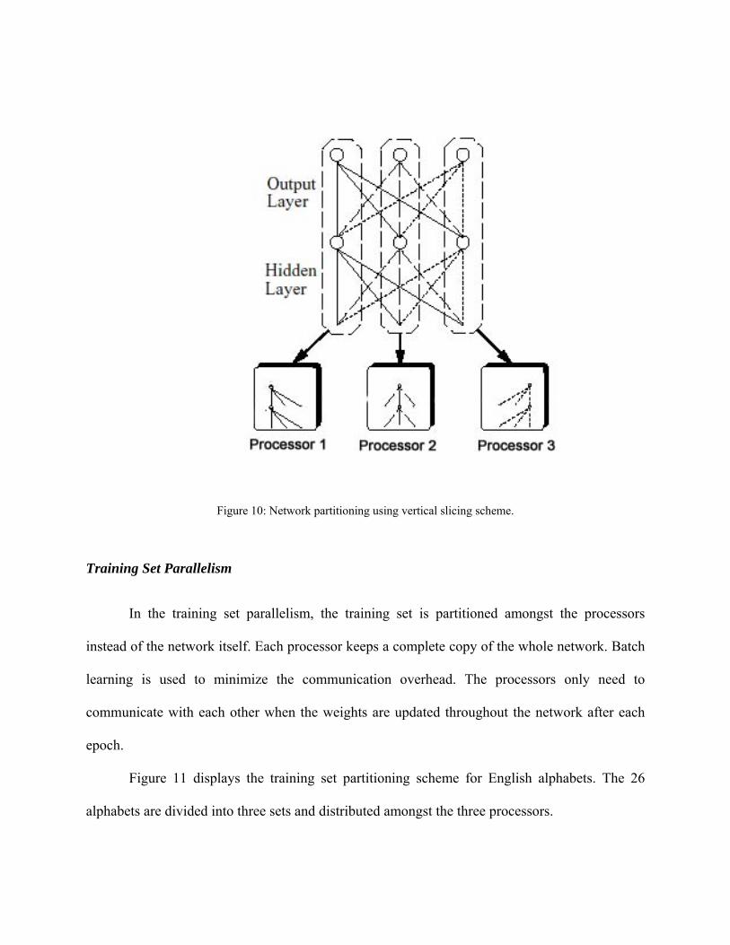
Figure 10: Network partitioning using vertical slicing scheme.
Training Set Parallelism
In the training set parallelism, the training set is partitioned amongst the processors
instead of the network itself. Each processor keeps a complete copy of the whole network. Batch
learning is used to minimize the communication overhead. The processors only need to
communicate with each other when the weights are updated throughout the network after each
epoch.
Figure 11 displays the training set partitioning scheme for English alphabets. The 26
alphabets are divided into three sets and distributed amongst the three processors.

Figure 11: Training set partitioning of English alphabets.
Parallel Backpropagation
Our parallel backpropagation system runs on a Beowulf cluster using CRLib [19, 20].
Because of the fast processors but slower I/O we had to choose such scheme for parallelism
which uses lesser interaction between processors in order to keep the communication overhead
low. Therefore we adopted training set partitioning scheme.
Algorithm
In the CRLib program one process is chosen as the root process. Besides usual
calculations for the neural network, the responsibilities of the root include:
• Reading the input data file and partitioning it amongst the processors.
• Receiving weight updates and errors from all the processes and adding them up to
get the total weight update.
• Broadcasting the update weights to all the processes.

• Checking for defined stopping criteria and sending the done signal to all the
processes in case training is finished.
The basic algorithm can be divided into two phases; setup and training.
• The setup phase consists of reading the input file and distributing data amongst
the processors. This time was observed to be almost constant with a slight
increase as the number of processors was increased.
• Training phase was the major phase that dominates the total execution time of the
algorithm.
The following notations are used in the description of the algorithm below.
PT total number of patterns
N total number of processors
K number of nodes in the input layer
J number of nodes in the hidden layer
I number of nodes in the output layer
xk(p) input for pattern p
yj2(p) calculated output for pattern p
di2(p) desired output for pattern p
yj1(p) hidden layer output for pattern p
wij2(t) current output layer weights
wjk1(t) current hidden layer weights
σi2(p) output layer error term for pattern p

σj1(p) hidden layer error term for pattern p
∆ wij2(t) current change in weight for output layer
∆ wjk1(t) current change in weight for hidden layer
∆ wij2(t-1) previous change in weight for output layer
∆ wjk1(t-1) previous change in weight for hidden layer
η learning rate
α momentum term
e(p) mean squared error for pattern p
ρ wij2(t) accumulated weight updates for output layer for current epoch
ρ wjk1(t) accumulated weight updates for hidden layer for current epoch
E(p) accumulated mean squared error for current epoch
∆ Wij2(t) total weight update for output layer at root for current epoch
∆ Wjk1(t) total weight update for hidden layer at root for current epoch
σ(t) total mean squared error at root for current epoch
The algorithm can be described as a step by step procedure as follows:
1.
a. If this is the root processor
i. Read the input file.
ii. Distribute the data amongst the processors
b. If this is not the root processor
i. Receive the data from root processor
2. Initialize the weights on each processor

3. Present the input pattern x(p) to the input layer.
4. Calculate the outputs at the hidden and output layers.
yj1(p) = g(neti
1(p)) = g[Σk=0Kwjk
1(t).xk(p)] 1 ≤ j ≤ J
yj2(p) = g(neti
2(p)) = g[Σj=0Jwij
2(t).yj1(p)] 1 ≤ i ≤ I
5. Calculate the error terms associated with output and hidden layers.
σi2(p) = g’(neti
2(p))[di2(p) – yi
2(p)] 1 ≤ i ≤ I
σj1(p) = g’(netj
1(p)) Σi=1Iwij
2(t). σi2(p) 1 ≤ j ≤ J
6. Calculate the weight updates for this pattern
∆ wij2(t) = η. σi
2(p). yj1(p) + α . ∆ wij
2 (t-1) 1 ≤ i ≤ I, 0 ≤ j ≤ J
∆ wjk1(t) = η. Σj
1(p). xk(p) + α . ∆ wjk1(t-1) 1 ≤ j ≤ J, 0 ≤ k ≤ K
7. Calculate the MSE for this pattern
e(p) = ½ [di2(p) – yi
2(p)]2
8. We distinguish two cases here
a. If p = PT
i. go to step 9
b. If p ≠ PT
i. Increase p
ii. Accumulate the weight update for this epoch
ρ wij2(t) = ρ wij
2(t) + ∆ wij2(t)
ρ wjk1(t) = ρ wjk
1(t) + ∆ wjk1(t)
iii. Accumulate the MSE for this epoch

E(p) = E(p) + e(p)
iv. Go to step 3
9.
a. If this is not the root processor
i. Send the calculated MSE and weight updates to the root processor.
b. If this is the root processor
i. Receive the MSE and weight updates from all the processors.
If this is the root processor perform steps 10 - 14, otherwise move to step 15
10. Calculate the total weights by adding all the weights received from each processor.
∆ Wij2(t) = Σn=1
N ρ wij2(t)
∆ Wjk1(t) = Σn=1
N ρ wjk1(t)
11. Calculate the total error
σ(t) = 1/N Σn=1N E(p)
12. Check to see if the total MSE is less than the required MSE
a. If yes
i. Set the done signal
ii. Go to step 15
b. If no
i. Go to step 13
13. Update the weights.
wij2(t) = wij
2(t) + ∆ Wij2(t) 1 ≤ i ≤ I, 0 ≤ j ≤ J
wik1(t) = wik
1(t) + ∆ Wjk1(t) 1 ≤ j ≤ J, 0 ≤ k ≤ K

14.
a. If this is the root processor
i. Broadcast the updated weights and done signal.
b. If this is not the root processor
i. Receive the updated weights and done signal from the root.
15. We now distinguish two cases
a. If done is set, training is considered complete.
b. If done is not set
i. Set p = 0
ii. Go to step 3.
Parallel Fuzzy ARTMAP
Fuzzy ARTMAP use fast match based learning as compared to the slow mismatch
learning by backpropagation [24]. In fast learning adaptive weights converge to equilibrium in
response to each input pattern [21]. As we discussed earlier a fast learning algorithm can further
benefits from applying high performance techniques, we parallelize the fuzzy ARTMAP
algorithm to acquire improved efficiency regarding the training time.
The same Beowulf cluster was used for experimentations with the parallel fuzzy
ARTMAP. Training set partitioning scheme was chosen to reduce the communication between
processes.
Our parallel implementation of the fuzzy ARTMAP algorithm take advantage of the
match based learning capability of the ART systems [21]. A central feature of all the ART

systems is a pattern matching process that compares an external input with the internal memory
of the system which represents some prototype stored patterns from a previous learning. Our
algorithm consists of two major steps. In the first step, each processor on the system is trained
with portion of the data it is assigned with. There is no communication between processors in
this step. When the training is complete, each processor has a set of stored patterns which are
learned during the training phase. In the second step, each processor sends its stored patterns to
one processor (root). Root is then trained on these stored patterns from every processor including
its own. The patterns learned at the end of the training at root are the prototype patterns
representing the whole dataset.
The basic algorithm can be divided into two sections; setup and training.
• The setup part consists of reading the input file and distributing data amongst the
processors. The file reading time was constant while the distribution time
increases with the number of processors.
• The second part was the training part. Since fuzzy ARTMAP is a fast learning
algorithm which is further speeded up by parallelization, training time was not the
major dominating phase of the total execution time for every case.
Algorithm
The following notations are used in the description of the algorithm below.
ARTa ART Module for inputs
ARTb ART Module for outputs
F1a matching layer in ARTa
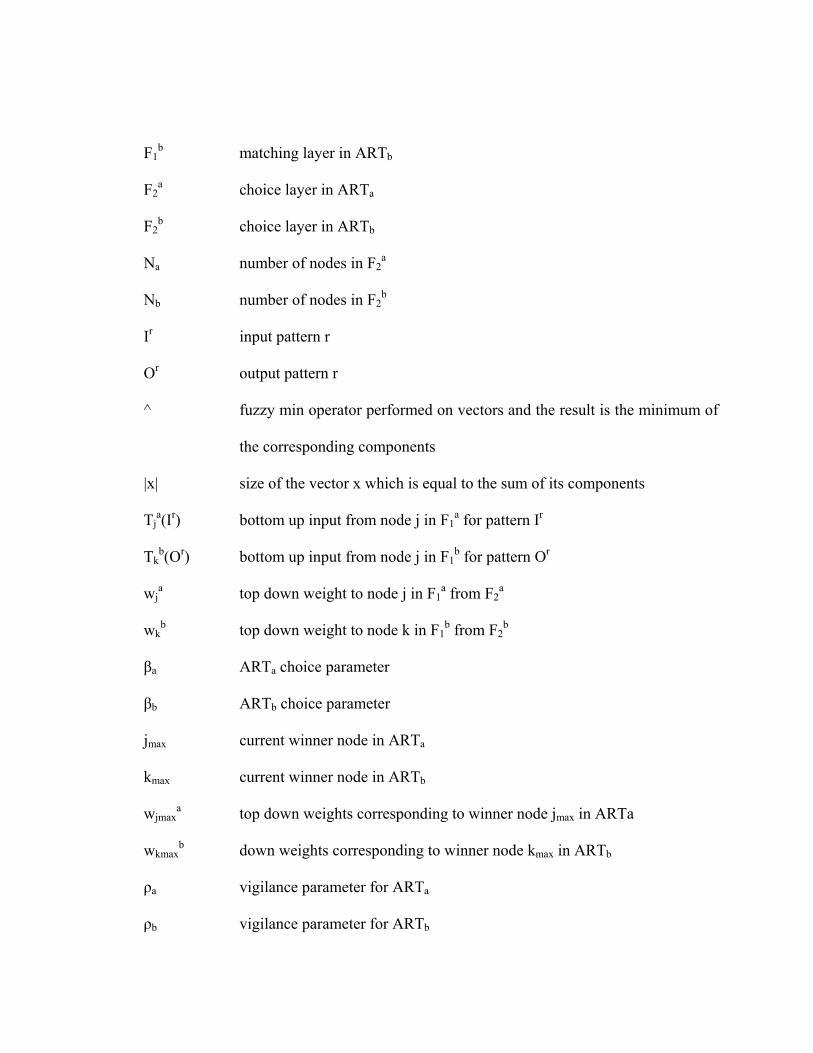
F1b matching layer in ARTb
F2a choice layer in ARTa
F2b choice layer in ARTb
Na number of nodes in F2a
Nb number of nodes in F2b
Ir input pattern r
Or output pattern r
^ fuzzy min operator performed on vectors and the result is the minimum of
the corresponding components
|x| size of the vector x which is equal to the sum of its components
Tja(Ir) bottom up input from node j in F1
a for pattern Ir
Tkb(Or) bottom up input from node j in F1
b for pattern Or
wja top down weight to node j in F1
a from F2a
wkb top down weight to node k in F1
b from F2b
βa ARTa choice parameter
βb ARTb choice parameter
jmax current winner node in ARTa
kmax current winner node in ARTb
wjmaxa top down weights corresponding to winner node jmax in ARTa
wkmaxb down weights corresponding to winner node kmax in ARTb
ρa vigilance parameter for ARTa
ρb vigilance parameter for ARTb

ε increment in the vigilance parameter
The modified fuzzy ARTMAP algorithm in a step by step procedure can be described as:
1.
a. If this is the root processor
i. Read the input file.
ii. Distribute the data amongst the processors
b. If this is not the root processor
i. Receive the data from root processor
2. Initialize the weight vectors corresponding to the uncommitted nodes in F2a and F2
b to all-
ones on each processor.
3. Present the input/output pair to the network and set the vigilance to base-line vigilance.
4. Calculate the bottom up inputs to all the Na nodes in F2a.
Tja(Ir) = (| Ir ^ wj
a | ) / (βa + | wja |)
5. Choose the node in F2a that receives the maximum input from F1
a. Assume its index is
jmax. Check to see if it satisfies the vigilance criteria. We now distinguish three cases:
a. If node jmax is uncommitted node, it satisfies the vigilance criteria in ARTa. Go to
step 6.
b. If node jmax is commited node and it satisfies the vigilance criteria, go to step 6. A
node jmax satisfies the vigilance criteria if
| Ir ^ wjmaxa | / | Ir | ≥ ρa
c. If node jmax does not satisfy the vigilance criteria, disqualify this node and go to
the beginning of step 5.

6. Now consider three cases:
a. If node jmax is an uncommitted node, designate the mapping of jmax in F2a to kmax
in F2b. kmax is found by executing the following steps:
i. Calculate the bottom up inputs to all the Nb nodes in F2b.
Tkb(Or) = (| Or ^ wk
b | ) / (βb + | wkb |)
ii. Choose the node in F2b that receives the maximum input from F1
b. Assume
its index is kmax. Check to see if it satisfies the vigilance criteria. We now
distinguish three cases:
1. If kmax is an uncommitted node, it satisfies the vigilance criteria.
Increase Nb by one by introducing a new uncommitted node in F2b
and initialize its top down weights to all-ones. Go to step 6(a) ii-4.
2. If kmax is commited node and it satisfies the vigilance criteria, go to
step step 6(a)ii-4. A node kmax satisfies the vigilance criteria if,
| Or ^ wkmaxb | / | Or | ≥ ρb
3. If kmax is commited node and it does not satisfy the vigilance
criteria, disqualify this node by setting Tkmax(Or ) = -1 and go to the
beginning of step 6(a) ii.
4. Now node jmax in F2a is mapped to node kmax in F2
b. The top-down
weights in ARTa and ARTb are updated.
wjmaxa = Ir ^ wjmax
a
wkmaxb = Or ^ wkmax
b

b. If node jmax is a commited node and due to prior learning this node is mapped to
node kmax and kmax satisfies the vigilance criteria, correct mapping is achieved
and weights in ARTa and ARTb are updated. If this is the last pattern in the
training set, go to step 7, otherwise go to step 3 and present the next in sequence
pattern.
c. If node jmax is a commited node and due to prior learning this node is mapped to
kmax and kmax does not satisfy vigilance criteria, disqualify jmax by setting Tjmax(Ir )
= -1, increase the vigilance criteria in ARTa and go to step 5.
| Ir ^ wjmaxa | / | Ir | + ε
7. After all the patterns are presented, consider two cases:
a. If in the previous list presentation, at least one component of the top-down weight
vectors was changed, go to step 3 and present the first pattern in the training set.
b. If in the previous list presentation, no weight changed occurred, the training is
finished. We now distinguish two cases.
i. If the training set was original patterns go to step 8.
ii. If the training set was stored patterns from all the processors and this
processor is root go to step 12.
8.
a. If this is the root processor
i. Receive the stored patterns from all the processors
b. If this is not the root processor
i. Send the stored patterns to the root processor

Steps 9-12 are only performed on the root processor.
9. Set the inputs and outputs to the stored pattern and their corresponding outputs
10. Initialize the weights vectors to all-ones and reset the F2a and F2
b layers.
11. Go to step 3.
12. Training is considered finished and the stored patterns represent the prototype patterns
from the whole dataset.

CHAPTER 4: EXPERIMENTAL RESULTS
The experiments were performed on the network traffic data generated by the MIT
Lincoln Labs for the 1998 DARPA Intrusion Detection Evaluation program. A version of this
data was also used in the 1999 KDD Intrusion Detection contest and is available from the UCI
KDD Archive [22]. Lincoln Labs artificially generated this data by simulating a military LAN
environment infused with different attacks. The data consists of network connection records
generated by TCP dump.
A network connection record is a set of information, such as duration, protocol type,
number of transmitted bytes etc, which represents a sequence of data flow to and from a well
defined source and target.
Each record in this data carry 41 different attributes and was marked as normal or attack,
with exact specification about the attack type. All the attacks fall into four main categories.
• DOS: denial-of-service, e.g. syn flood;
• R2L: unauthorized access from a remote machine, e.g. guessing password;
• U2R: unauthorized access to local superuser (root) privileges, e.g., various
buffer overflow attacks;
• probing: surveillance and other probing, e.g., port scanning.
The training dataset contains 4848429 records while the test dataset had 311029 records.
Running the full dataset on a single processor suffers from memory problems and the speed
further slowed down. To encounter this problem we used a reduced 10% dataset of the original
dataset also for our experiments to measure the training times especially for one processor. The

reduced dataset has 494020 patterns and this dataset is the most widely used dataset for intrusion
detection research. There were 24 different types of attacks along with the normal patterns in the
training data. Test data has 14 additional attacks that were not found in the training data.
The 24 attack types found in the training dataset are:
Table 1: Attack types in the training data set
S.No Attack Name Category1 Back DoS 2 buffer_overflow U2R 3 ftp_write R2L 4 guess_passwd R2L 5 imap R2L 6 ipsweep Probe 7 land DoS 8 loadmodule U2R 9 multihop R2L 10 neptune DoS 11 nmap Probe 12 perl U2R 13 phf R2L 14 pod DoS 15 portsweep Probe 16 rootkit U2R 17 satan Probe 18 smurf DoS 19 spy R2L 20 teardrop DoS 21 werezclient R2L 22 werezmaster R2L 23 snmpgetattack R2L 24 xlock R2L
The training data consists of 41 features which can be divided into 3 categories.
1. Basic features of individual TCP connections. 2. Content features within a connection suggested by domain knowledge.

3. Traffic features computed using 2 second time window. A complete listing of the set of features defined for the connection records is given in the
three tables below.
Table 2: Basic features of individual TCP connections
feature name description type duration length (number of seconds) of the connection continuousprotocol_type type of the protocol, e.g. tcp, udp, etc. discrete service network service on the destination, e.g., http, telnet, etc. discrete src_bytes number of data bytes from source to destination continuousdst_bytes number of data bytes from destination to source continuousflag normal or error status of the connection discrete land 1 if connection is from/to the same host/port; 0 otherwise discrete wrong_fragment number of ``wrong'' fragments continuousurgent number of urgent packets continuous
Table 3: Content features within a connection suggested by domain knowledge
feature name description type hot number of ``hot'' indicators continuousnum_failed_logins number of failed login attempts continuouslogged_in 1 if successfully logged in; 0 otherwise discrete num_compromised number of ``compromised'' conditions continuousroot_shell 1 if root shell is obtained; 0 otherwise discrete su_attempted 1 if ``su root'' command attempted; 0 otherwise discrete num_root number of ``root'' accesses continuousnum_file_creations number of file creation operations continuousnum_shells number of shell prompts continuousnum_access_files number of operations on access control files continuousnum_outbound_cmds number of outbound commands in an ftp session continuousis_hot_login 1 if the login belongs to the ``hot'' list; 0 otherwise discrete is_guest_login 1 if the login is a ``guest''login; 0 otherwise discrete

Table 4: Features computed using a two-second time window.
feature name description type
count number of connections to the same host as the current connection in the past two seconds continuous
Note: The following features refer to these same-host connections.
serror_rate % of connections that have ``SYN'' errors continuousrerror_rate % of connections that have ``REJ'' errors continuoussame_srv_rate % of connections to the same service continuousdiff_srv_rate % of connections to different services continuous
srv_count number of connections to the same service as the current connection in the past two seconds continuous
Note: The following features refer to these same-service connections.
srv_serror_rate % of connections that have ``SYN'' errors continuoussrv_rerror_rate % of connections that have ``REJ'' errors continuoussrv_diff_host_rate % of connections to different hosts continuous
Data preprocessing
Data preprocessing can be described as any type of processing performed on the raw data
to prepare it for any other processing procedure. Data preprocessing is an important step in data
mining. It transforms the data into a format that is acceptable to the actual data processing
algorithm e.g. a neural network.
The KDD dataset has two types of attribute; discrete and symbolic. The discrete attributes
can be in the form of a Boolean value or it might represent a symbolic denomination like
protocol type can have tcp or udp as its values. These symbolic values were transformed into
appropriate numerical representations. A requirement for fuzzy ARTMAP is that the input values
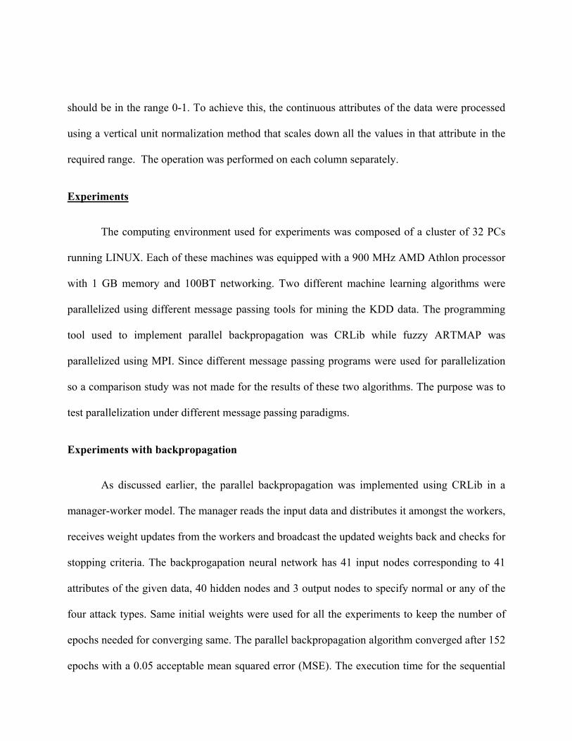
should be in the range 0-1. To achieve this, the continuous attributes of the data were processed
using a vertical unit normalization method that scales down all the values in that attribute in the
required range. The operation was performed on each column separately.
Experiments
The computing environment used for experiments was composed of a cluster of 32 PCs
running LINUX. Each of these machines was equipped with a 900 MHz AMD Athlon processor
with 1 GB memory and 100BT networking. Two different machine learning algorithms were
parallelized using different message passing tools for mining the KDD data. The programming
tool used to implement parallel backpropagation was CRLib while fuzzy ARTMAP was
parallelized using MPI. Since different message passing programs were used for parallelization
so a comparison study was not made for the results of these two algorithms. The purpose was to
test parallelization under different message passing paradigms.
Experiments with backpropagation
As discussed earlier, the parallel backpropagation was implemented using CRLib in a
manager-worker model. The manager reads the input data and distributes it amongst the workers,
receives weight updates from the workers and broadcast the updated weights back and checks for
stopping criteria. The backprogapation neural network has 41 input nodes corresponding to 41
attributes of the given data, 40 hidden nodes and 3 output nodes to specify normal or any of the
four attack types. Same initial weights were used for all the experiments to keep the number of
epochs needed for converging same. The parallel backpropagation algorithm converged after 152
epochs with a 0.05 acceptable mean squared error (MSE). The execution time for the sequential

version was 68 hours and 37 minutes while the parallel version reduced this time to 1 hour and
33 minutes using a 32 node cluster. The speedup achieved was 43.9 which is a linear gain. As a
measure of performance, we are reporting execution time for single epoch, as this is the most
common way to report the speedup of a parallel neural network.
Table 5: Training times for a single epoch for parallel backpropagation for full dataset
No of processors 1 2 4 8 16 32
Execution time (sec) 1625 587 298 150 76 38
1
10
100
1000
10000
1 2 4 8 16 32No of Processors
Exec
utio
n tim
e (s
ec)
Figure 12: Execution times for backpropagation for a single epoch in logarithmic scale for full dataset.

There is a setup time also involved as discussed previously in the parallel algorithm that
consists of input data reading and distribution times. This setup time was observed to be almost
constant regardless of the number of processors with the exception of the serial version with only
one processor. The reason for constant time is that the root processor read the data and
distributed it amongst the processors. If the number of processors is small, larger partitions were
transferred over the network to small number of processors. If the number of processors is large,
smaller partitions were transferred to a large number of processors. In any case the total amount
of data transferred over the network remains the same.
Table 6: Setup times for parallel backpropagation for full dataset
No of processors 2 4 8 16 32
Execution time (sec) 625 433 422 415 432
Training the network with the full dataset on a single machine suffers from memory
problems. Loading the full dataset into memory resulted in segmentation faults. We had to
partition the dataset and load each partition one at a time into memory during the training.
Table 6 doesn’t include the setup time for one processor for this reason. The input file
was read continuously for each epoch. This also explains the relatively larger value for execution
time for one processor in table 5. In this case execution time includes both setup time and
training time.

To remedy this problem we used the 10% dataset to have a fairer speed comparison as the
number of processors is increased. Nevertheless it again proves the limitation of hardware and
advantages of using parallel computing for our work.
Table 7: Training times for a single epoch for parallel backpropagation for 10% dataset
No of processors 1 2 4 8 16 32
Execution time (sec) 110 59 30 15 8 4
1
10
100
1000
1 2 4 8 16 32No of Processors
Exec
utio
n tim
e (s
ec)
Figure 13: Execution times for backpropagation for a single epoch in logarithmic scale for 10% dataset
The setup times for 10% dataset are documented in table 8.

Table 8: Setup times for parallel backpropagation for 10% dataset
No of processors 1 2 4 8 16 32
Setup time (sec) 42.1 42.1 41.9 41.9 41.7 41.8
For the training dataset, the backpropagation network demonstrated 98.36% classification
rate. The false positive rate was 1.26% and the false negative rate was 0.38%.
The testing dataset contained 14 new attacks which were not present in the training
dataset. This would test the system in a real time scenario with unknown attacks. The neural
network generalization capability enabled it to predict 81.37% of the patterns correctly. False
positive rate was 1.28% while the false negative rate was 17.35%. The negative false alarm rate
indicates that most of the unknown attacks were going unnoticed. Usually a neural network is
retrained when new patterns are discovered to include those patterns into its learning paradigm.
Table 9: Performance of parallel backpropagation algorithm
Training Data Test Data Classification Rate 98.36% 81.37% False Negatives 0.38% 17.35% False Positives 1.26% 1.28%
Experiments with fuzzy ARTMAP
The fuzzy ARTMAP system also follows the manager-worker model as
backpropagationas does. The manager duties include reading and distributing the input data,

receiving stored patterns from workers when they finished their training, and training on stored
patterns. In addition manager also performs worker operations.
The fuzzy ARTMAP system consists of two ART modules; ARTa and ARTb. The 41
input features were fed to the ARTa module while the corresponding output was given to the
ARTb module. To achieve parallelization, training set partitioning scheme was used. Fuzzy
ARTMAP uses fast match based learning and it usually converges in few epochs.
The parallel algorithm has two phases. In the first phase each network is trained
separately on its assigned partition of the full dataset. The second phase consists of training one
network with the prototype patterns learned in the first phase by all the networks. With
appropriately chosen parameters, the first phase always dominates the execution time. Since
separate networks are trained with separate datasets in the first phase we consider average
training time as a measure of the execution time.
The algorithm converged in just 2 epochs with the average training time of 92 seconds on
a 32 node cluster.
Table 10: Training times for a single epoch on parallel fuzzy ARTMAP for full dataset
No of processors 1 2 4 8 16 32
Execution time (sec) 1851 805 392 192 95 46

1
10
100
1000
10000
1 2 4 8 16 32No of Processors
Exec
utio
n tim
e (s
ec)
Figure 14: Training times for fuzzy ARTMAP for a single epoch in logarithmic scale for full dataset
The setup time on fuzzy ARTMAP was slightly different from the backpropagation
implementation because it uses a different manager-worker approach. Since manager performs
worker operations also in addition to its duties, the distribution time varies as the number of
processors varies. The amount of data to be distributed, increases as the number of processor
increases. The reason being the manager keeps its partition of data and distribute the rest
amongst the workers. As the number of workers increases, the partitions become small so
manager keep a small partition and distribute the rest.

Table 11: Setup times for fuzzy ARTMAP for full dataset.
No of processors 2 4 8 16 32
Setup time (sec) 330 368 397 402 405
Again, single machine suffers from memory problems with the full dataset. Segmentation
faults were observed while loading the full dataset into memory. So, we partitioned the dataset
and loaded each partition one at a time into memory during the training.
Table 11 doesn’t include time for one processor because execution time for an epoch
includes setup time in addition to the training time. This also explains the large value for epoch
execution time for one processor in table 10.
We performed experiments with the 10% dataset on the fuzzy ARTMAP also to get a
balanced view of training times without memory problems. This showed that an almost linear
speedup was obtained as the number of processors was increased. The times reflected in the table
are average times for one epoch. We used the notion of average time here because in such a
parallel fuzzy ARTMAP system, not every processor is executing the same number of steps
every time. A closer look at the algorithm revealed that winner node selection step might take
more iteration on some processor depending upon the dataset it received. This iteration is nested
within the operation of each epoch and hence a change in its value will result in a variation in the
epoch time.

Table 12: Training times for a single epoch on parallel fuzzy ARTMAP for 10% dataset
No of processors 1 2 4 8 16 32
Execution time (sec) 157 74 36 18 8 4
1
10
100
1000
1 2 4 8 16 32No of Processors
Exec
utio
n tim
e (s
ec)
Figure 15: Training times for fuzzy ARTMAP for a single epoch in logarithmic scale for 10% dataset
For the 10% dataset the total execution time for the algorithm was dominated by the
setup time as the number of processors increases as indicated by table 13. The setup time
includes input file reading and data distribution times.

Table 13: Distribution times on parallel fuzzy ARTMAP for 10% dataset
No of processors 1 2 4 8 16 32
Setup time (sec) 26 33 37 39 41 41
Testing on the training data gives 80.14 % classification rate. The false positive and
negative rates were 0%. Test data gave an 80.52% success rate with 0.0% false negative rate and
19.48% false positive rate. A high false positive rate indicates that a number of normal patterns
were detected as attacks. Detection algorithms of all kind have a tendency to create false
positives and negatives. A false negative is a more serious concern than a false positive because
a false negative means that an attack has gone unnoticed while false positive flags a normal
activity as attack which is not considered a security threat.
Table 14: Performance of parallel fuzzy ARTMAP algorithm
Training Data Test Data Classification Rate 80.14% 80.52% False Negatives 0.0% 0.0% False Positives 19.86% 19.48%

CHAPTER 5: CONCLUSIONS
We introduced a new strategy to address the issue of scalability of learning algorithms for
intrusion detection. Our research focuses on using high performance distributed computing
techniques to scale existing data mining algorithms to deal with large datasets for problems in
intrusion detection. The scalability issue is widely ignored in the intrusion detection research. As
a result most of the research projects are restricted to use smaller datasets which may not reflect
real-world scenario of dealing with ever increasing audit files.
We developed parallel backpropagation and parallel fuzzy ARTMAP algorithms to
analyze network traffic data. With the help of our parallel algorithms we were able to investigate
much larger set of patterns than their sequential versions would allow. Out experimental results
showed that the developed parallel model can significantly reduce training time in the neural
networks algorithms, achieving a linear speedup using a cluster computing environment, without
sacrificing accuracy in classification and prediction rate.
We showed how intrusion detection can benefit from high performance data mining
techniques. For our experiments we came up with a parallelized version of the fuzzy ARTMAP
algorithm for cluster environment.
Improving the parallel fuzzy ARTMAP algorithm we developed is an open area for
future research. Experiments with other datasets can be performed using our parallel models.
Further research can be done in this area by applying the same parallel computing techniques to
other data mining algorithms.

LIST OF REFERENCES
[1] CERT/CC Statistics 1988-2003, http://www.cert.org/stats/cert_stats.html
[2] Jones, Anita K., Sielken, Robert S., “Computer system intrusion detection: A survey”,
Technical Report, Computer Science Dept., University of Virginia, 1999.
[3] Koziol, Jack, “Intrusion detection with Snort”, Sams Publishing, 2003.
[4] Bace, Rebecca Gurley, Intrusion detection”, Macmillan Technical Publishing, 2000.
[5] Crothers, Tim, “Implementing intrusion detection systems”, Wiley Publishing, Inc., 2003.
[6] Mohammadian, M., “Intelligent Agents for Data Mining and Information Retrieval,”
Hershey, PA Idea Group Publishing, 2004
[7] Wang, J., “Data mining: Opportunities and challenges,” Idea Group Publishing, September,
2003.
[8] McCulloch, W.S., and Pitts, W., “A logical calculus of the ideas immanent in nervous
activity,” Bulletin of Mathematical Biophysics, vol. 5, pp. 115-133, 1943.
[9] Haykin, Simon, “Neural networks, A comprehensive foundation”, Macmillan College
Publishing Company, Inc.
[10] Christodoulou, C., Georgiopoulos, M., “Applications of Neural Networks in
Electromagnetics”, Artech House.
[11] Carpenter, Gail A. Grossberg, S., Markuzon, N., Reynolds, John H., Rosen, David B.,
“Fuzzy ARTMAP: An adaptive resonance architecture for incremental learning of analog maps”,
International Joint Conference on Neural Networks, vol. 3, pp. 302-314, June 1992.

[12] Hussam, O. Mousa, “A survey and analysis of Neural Network approaches to Intrusion
Detection” November 2002.
[13] Lee, J., Siddiqui, M., “High performance data mining for intrusion detection”, submitted to
IEEE International Symposium on High-Performance Distributed Computing, 2004.
[14] Lee, W., Stolfo, Salvatore J., “Data mining approaches for intrusion detection”, Proceedings
of the 2nd USENIX Security Symposium, 1998.
[15] Ye, N., Emran, S. M., Chen, Q., Vilbert, S. “Multivariate statistical analysis of audit trails
for host-based intrusion detection”, IEEE Transactions on Computers, vol. 51, no. 7, pp. 810-
820, 2002.
[16] Lee, W., “Applying data mining to intrusion detection: the quest for automation, efficiency
and credibility”, ACM SIGKDD Explorations Newsletter, vol. 4 no. 2, pp. 35-42.
[17] Riedmiller, M., Braun, H., “RProp – A fast adaptive learning algorithm”, Proceedings of
ISCIS VII.
[18] Saratchandran, P., Sundarajan, N., Foo, Shou King, “Parallel implementations of
backpropagation neural networks on transputer – A study of training set parallelism”, Progress in
Neural Processings 3.
[19] Lee, J., Chapin, S. J., Taylor, S., “Computational Resiliency”, Journal of Quality and
Reliability Engineering International, vol. 18, no. 3, pp 185-199, 2002.
[20] Lee, J., Chapin, S., Taylor, S., “Reliable heterogeneous applications”, IEEE Transactions on
Reliability, vol. 52, no. 3, pp. 330-339, 2003.
[21] Carpenter, G. A., Grossberg, S., “Adaptive resonance theory”, The Handbook of Brain
Theory and Neural Networks, 2nd ed. MIT press, April, 2002.
[22] KDD Cup 1999 Data, http://kdd.ics.uci.edu/databases/kddcup99/kddcup99.html
[23] Torresen, J. and Tomita, S., “A Review of Parallel Implementations of Backpropagation
Neural Networks”. Chapter 2 in the book by N. Sundararajan and P. Saratchandran (editors):
Parallel Architectures for Artificial Neural Networks, IEEE CS Press, 1998.
[24] Carpenter, G. A., Grossberg, S., and Reynolds, J., “ARTMAP: A self-organizing neural
network architecture for fast supervised learning and pattern recognition,” Proceedings of
International Joint Conference on Neural Networks, vol. 1, pp. 863-868.
[25] Axelsson, S., “Intrusion detection systems: A survey and taxonomy”, Technical Report, 99-
15 Dept. of Computer Engineering, Chalmers University, March 2000.
[26] Mukkamala, S. and Sung, A. H., “A comparative study of techniques for intrusion
detection,” 15th IEEE International Conference on Tools with Artificial Intelligence (ICTAI'03),
November 03 - 05, 2003, Sacramento, California, USA, pp 570.
[27] Drucker, H. and Cun, Y. L., “Improving generalization performance using double
backpropagation,” IEEE Transactions on Neural Networks, vol. 3, no. 6, pp. 991-997, 1992.
[28] Cun, Y. L. et. al., “Backpropagation applied to handwritten zip code recognition,” Neural
Computation, vol. 1, no. 4, pp. 541-551, 1989.
[29] Waibel, A., “Consonant recognition by modular construction of large phonetic time-delay
neural networks,” Advances in Neural Information Processing Systems, pp. 215-223, 1989.
[30] Sheng Ma, C. J. and Farmer, J., “An efficient EM-based training algorithm for feed forward
neural networks,” Neural Networks, vol. 10, no. 2, pp. 243-256, 1997.

[31] Osowski, P. B. S., and Stodoloski, M., “Fast second order learning algorithms for
feedforward neural networks and its applications,” Neural Networks, vol. 9, no. 9, pp. 1583-
1596, 1996.
[32] Geist, G. A., “Cluster computing: The wave of the future?”, Oak Ridge National
Laboratory, May 17, 1994.
[33] Sterling, T., Salmon, J., Becker, D. J., Savarese, D. S., “How to build a Beowulf: A Guide to
the Implementation and Application of PC Clusters,” The MIT press, May 1999.
[34] Sterling, T. L., “How to Build a Beowulf: A Guide to the Implementation and Application
of PC Clusters,” Cambridge, Mass MIT Press, 1999.
[35] Message passing interface forum, “MPI: A Message-Passing Interface Standard,” Technical
Report, University of Tennessee, Knoxville, Tennessee, May 1994.
[36] Sunderam, V. S., “PVM: A framework for parallel distributed computing,” Concurrency:
Practice and Experience, vol. 2, no. 4, pp. 315-339, Dec, 1990.
[37] Frasconi, P., Gori, M., and Tesi, A., “Successes and failures of backpropagation: A
theoretical investigation,” In Omidvar, O., editor, Progress in Neural Networks, pp. 205-242.
Ablex Publishing.
[38] Werbos, P. J., “Beyond regression: New tools for prediction and analysis in the behavioral
sciences,” PhD Dissertation, Committee on Applied Mathematics, Harvard University,
Cambridge, MA, November 1974.
[39] Klimasauskas, C., “Taking backpropagation to the extreme: A master shares his secrets,”
PC AI magazine, vol. 16, no. 1, pp. 31-35 Jan/Feb 2002.

[40] Carpenter, G. A., Grossberg, S., “The art of adaptive pattern recognition by a self-
organizing neural network,” IEEE Computer, vol. 21, no. 3, pp. 77-88, March 1988.
[41] Porass, P. A., Neumann, P. G., “EMERALD, Event monitoring enabling responses to
anomalous live disturbances,” Proceedings of the 20th National Information Systems Security
Conference, pp. 353-365, October, 1997.
[42] Lunt, T. F., Jagannathan, R., Lee, R., Listgarten, S., Edwards, D. L., Neumann, P. G., Javitz,
H. S., and Valdes A., “IDES: The enhanced prototype, A real time intrusion detection system,”
Technical Report, SRI Project 4185-010, SRI-CSL-88-12, October 1988.
[43] Anderson, D., Frivold, T., Valdes, A., “Next-generation intrusion-detection expert system
(NIDES),” Technical Report, SRI-CSL-95-07, May 1995.
[44] Sebring, M. M., Shellhouse, E., Hanna, M. E., Whitehurst, R. A., “Expert systems in
intrusion detection: A case study,” Proceedings of the 11th National Computer Security
Conference, pp 74-81, October 17-20, 1988.
[45] Kim, G. H., Spafford, E. H., “The design and implementation of Tripwire: A file system
integrity checker,” Proceedings of the 2nd ACM Conference on Computer and Communication
Security, pp. 18-29, 1994.
[46] White, G., Pooch, V., “Cooperating security managers: Distributed intrusion detection
systems,” Computer and Security, vol. 15, no. 5, pp. 441-450, 1996.
[47] Chen, S. S., Cheung, S., Crawford, R., Dilger, M., Frank, J., Haogland, J., Levitt, K., Wee,
C., Yip, R., Zerkle, D., “GrIDS – A graph based intrusion detection system for large networks,”,
Proceedings of the 19th National Information Systems Security Conference, 1996.
[48] Heberlein, T,. Dias, G., Levitt, K., Mukherjee, B., Wood, J., Wolber, D., “A network
security monitor,” Proceedings of the 1990 IEEE Symposium on Research in Security and
Privacy, pp. 296-304, 1990.
[49] Ryan, J., Lin, M-J., Miikkulainen, R., “Intrusion detection with neural networks,” Advances
in Neural Information Processing Systems 10, Cambridge, MA: MIT Press.
[50] Lee, W., Stolfo, S. J., “Combining Knowledge Discovery and Knowledge Engineering to
Build IDSs,” Proceedings of the Second International Workshop on the Recent Advances in
Intrusion Detection (RAID'99), October 1999.
[51] Barbara, D., Couto, J., Jajodia, S., Popyack, L., Wu, N., “ADAM: Detecting intrusions by
data mining,” Proceedings of the 2001 IEEE Workshop on Information Assurance and Security,
June, 2001.
[52] Vaccaro, H. S., Liepins, G. E., “Detection of anomalous computer session activity,”
Proceedings of the 1999 IEEE Symposium on Security and Privacy, pp. 280-289, May, 1989.
[53] Tan, K., “The application of neural networks to Unix computer security,” Proceedings of the
International Conference on Neural Networks, 1995.
[54] Charron, F., Ghosh, A., Wanken, J., “Detecting anomalous and unknown intrusions against
programs,” Proceedings of 14th Annual Computer Security Applications Conference, pp. 259-
267, 1998.
[55] Jorgensen, J., Manikopolous, C., Li, J., Zhang, Z., “A hierarchical anomaly network
intrusion detection system using neural network classification,” Proceedings of the 2001 IEEE
Workshop on Information Assurance and Security, June 2001.

[56] Cannady, J., “Artificial neural networks for misuse detection,” Proceedings of the 1998
National Information Systems Security Conference (NISSC'98) October, 1998.
[57] Ghosh, A., Schwartzbard, A., “A study in using neural networks for anomaly and misuse
detection,” Proceedings of the 8th USENIX Security Symposium, pp. 141151, 1999.
[58] Hatonen, K., Hoglund, A., Sorvari, A., “A computer hosed-based user anomaly detection
system using the self-organizing maps,” Proceedings of the IEEE-INNS-ENNS International
Joint Conference on Neural Networks, vol. 5, pp 411-416, 2000.
[59] Heywood, M., Lichodzijewski, P., Zincir-Heywood, N., “Host-based intrusion detection
using self-organizing maps,” IEEE International Joint Conference on Neural Networks, May
2002.
[60] Ghosh, A., Schatz, M., Schwartzbard, A., “Learning program behavior profiles for intrusion
detection,” Proceedings of the 1st USENIX Workshop on Intrusion Detection and Network
Monitoring, pp. 51-62, April, 1999.
[61] Elman, J. L., “Finding structure in time,” Cognitive Science, vol. 14, pp. 179-211, 1990.